Embed Size (px)
Citation preview

NATIONAL COOPERATIVE HIGHWAY RESEARCH PROGRAM
DRAFT FINAL REPORT
EVALUATION OF ABUTMENT-SCOUR EQUATIONS FROM NCHRP PROJECTS 24-15(2) AND 24-20
USING LABORATORY AND FIELD DATA
NCHRP 24-20(2)
Stephen T. Benedict U.S. Geological Survey
Clemson, South Carolina 29631 USA
Subject Areas Highway and Facility Design • Bridges, Other Structures, and Hydraulic and Hydrology •Soils, Geology, and
Foundations • Materials and Construction
Research Sponsored by the American Association of State Highway and Transportation Officials in Cooperation with the Federal Highway Administration
TRANSPORTATION RESEARCH BOARD
WASHINGTON, D.C. June 2015
www.TRB.org

ii
EVALUATION OF ABUTMENT-SCOUR EQUATIONS FROM NCHRP PROJECTS 24-15(2) AND 24-20
USING LABORATORY AND FIELD DATA
EXECUTIVE SUMMARY
Problem Statement
The National Cooperative Highway Research Program (NCHRP) sponsored several projects for
the development of new abutment-scour prediction methods in cohesive and non-cohesive
sediments. These projects include:
1. NCHRP Project 24-15(2): Abutment Scour in Cohesive Soils1
2. NCHRP Project 24-20 Prediction of Scour at Bridge Abutments2
The NCHRP 24-15(2) and NCHRP 24-20 Projects represent extensive efforts to develop new
methods for predicting abutment scour, and with the completion of these investigations, there is a
need to test and evaluate their performance with field data. This analysis will help identify
strengths, weaknesses, and limitations associated with the newly developed scour prediction
methods, and will provide guidance to the practitioner for the application of these methods.
Project Objectives
The primary objectives of this investigation were to test and evaluate the performance of the
abutment-scour prediction methods developed in the NCHRP Projects 24-15(2) and 24-20, using
field measurements collected by the U.S. Geological Survey (USGS). To confirm prediction
patterns observed in the field data, laboratory measurements from previous investigations also
were applied to the newly developed methods. Results from the analysis were used to identify
1 Briaud, J.-L., Chen, H.-C., Chang, K.-A., Oh, S.J., and Chen, X. (2009). "Abutment Scour in Cohesive Material." NCHRP Report 24-15(2), Transportation Research Board, National Research Council, Washington, D.C. 2 Ettema, R., Nakato, T., and Muste, N. (2010). “Estimation of scour depth at bridge abutments.” Draft final report, NCHRP Report 24-20, National Cooperative Highway Research Program, Transportation Research Board, Washington, D.C.
iii
performance characteristics for each scour prediction method, note potential ways to improve
performance, and provide limited guidance to the practitioner for application of these methods.
Additionally this investigation aligns with a recommendation from NCHRP Project 24-27(02), a
review of the state of knowledge regarding abutment scour, that more data on abutment scour be
obtained and used to illuminate scour and evaluate methods for estimating scour depth.
Field and Laboratory Data
A literature review was done to identify potential sources of abutment-scour data, and selected
data, including 329 field and 514 laboratory measurements of abutment scour, were compiled
into a database. All of the field data were collected by the USGS and included 15 measurements
from the USGS National Bridge Scour Database3, 92 measurements from the moderate-gradient
streams of the South Carolina Piedmont having cohesive sediments4, 106 measurements from
the low-gradient streams of the South Carolina Coastal Plain (none are tidally influenced)
generally having sandy4, non-cohesive sediments, 93 measurements from the small, steep-
gradient streams of Maine having coarse sediments5, and 23 measurements from the low-
gradient streams of the Alabama Black Prairie Belt having cohesive sediments6. Most of these
data are historical scour measurements, similar to post-flood measurements, and are assumed to
represent the maximum abutment-scour depth that has occurred at the bridge since construction.
The field data are largely associated with clear-water scour conditions where sediments do not
refill the scour holes as flood waters recede, making them appropriate sites for historical scour
measurements. Because the scour measurements were made during low-flow conditions, one-
dimensional flow models were used to estimate the hydraulic properties. The measurement
characteristics associated with the field data (post flood) and the estimated hydraulics will
3 U.S. Geological Survey (2001). “National bridge scour database.” (http://water.usgs.gov/ osw/techniques/bs/BSDMS/index.html). 4 Benedict, S.T. (2003). “Clear-water abutment and contraction scour in the coastal plain and Piedmont provinces of South Carolina, 1996-99.” Water-Resources Investigations Report 03-4064, U.S. Geological Survey, Columbia, South Carolina. 5 Lombard, P.J., and Hodgkins, G.A. (2008). “Comparison of observed and predicted abutment scour at selected bridges in Maine.” Scientific Investigations Report 2008–5099, U.S. Geological Survey, Reston, VA. 6 Lee, K.G., and Hedgecock, T.S. (2008). “Clear-water contraction scour at selected bridge sites in the Black Prairie Belt of the Coastal Plain in Alabama, 2006.” Scientific Investigations Report 2007–5260 U.S. Geological Survey, Reston, VA.
iv
introduce some error into these measurements, making them less than ideal. It also is notable
that field conditions associated with the USGS field data will frequently deviate from the simple
models of the laboratory; therefore, the scour patterns in the laboratory and field data will differ
in some measure. In particular, the small to moderate drainage areas associated with most of the
USGS field data will tend to have peak-flow durations lasting only hours, likely preventing the
attainment of equilibrium abutment-scour depths comparable to those of the laboratory, where
peak flows may continue for days. Additionally, sediments in the field are typically non-uniform
in grain size and often have some measure of cohesion. Furthermore, field sediments often have
subsurface scour-resistant layers that impede or limit scour. These field characteristics are
distinctly different from the non-cohesive sediments of the laboratory and will tend to reduce
scour depth. The limitations and characteristics associated with the USGS field data make these
data less than ideal for evaluating laboratory-derived scour prediction equations. While the
limitations are acknowledged, it is currently (2015) the best available set of field data, and the
large number of measurements (329) should be sufficient to gain insights into the general trends
of abutment scour in the field setting.
In addition to field data, 514 laboratory measurements of abutment scour from selected authors,
including 359 measurements from Palaviccini7, 74 measurements from Sturm8, 19
measurements from the NCHRP 24-15(2) investigation1, and 62 measurements from the
NCHRP 24-20 investigation2, were incorporated into the database. The Palaviccini data consist
of measurements of live-bed and clear-water abutment scour in non-cohesive sediments
compiled from selected investigations conducted prior to 1990. The measurements were
collected in rectangular flumes with rigid abutment models. The Sturm data consist of clear-
water abutment scour in non-cohesive sediments collected in compound channels with rigid
abutment models. The NCHRP 24-15(2) data consist of clear-water abutment scour in cohesive
sediments collected in compound and rectangular channels with rigid abutment models. The
NCHRP 24-20 data consist of live-bed and clear-water abutment scour in non-cohesive
sediments collected in compound and rectangular channels. The NCHRP 24-20 investigation
7 Palaviccini, M. (1993). “Predictor model for bridge abutments. PhD Thesis, The Catholic University of America, Washington, D.C. 8 Sturm, T.W. (2004). “Enhanced abutment scour studies for compound channels.” Report No. FHWA-RD-99-156, Federal Highway Administration, McLean, VA.
v
used a combination of erodible and non-erodible floodplains, embankments, and abutment
substructures thought to better represent field conditions, and as such, are distinctly different
from the other data. The varying characteristics of the laboratory data will influence their
performance when applied to scour prediction equations, and this should be kept in mind when
reviewing the results of this investigation.
Comparison of Dimensionless Variables for Field and Laboratory
Data
Scour prediction equations developed from small-scale laboratory investigations are typically
scaled to the field through the development of equations associated with dimensionless variables.
To assure the success of a laboratory-derived equation, the range of the dimensionless variables
associated with the laboratory data should approximate the typical range found in the field. To
gain perspective, percentile plots of selected dimensionless variables that are commonly used in
the analysis of abutment scour were developed for the field and laboratory data. The
dimensionless variables included relative abutment length (L/y1), relative scour depth (ysadj/y1)
adjusted for abutment shape, unit discharge ratio (q2/q1), relative sediment size (L/D50), the
approach Froude number (Fr1), and the ratio of embankment length blocking flow to the
floodplain width (L/Bf). The percentile plots helped identify typical ranges associated with
selected explanatory variables for the laboratory and field data. It was notable that the laboratory
data did not include the higher range of embankment lengths and flow contractions found in the
field where potential for scour is greatest, indicating that the equations derived from the
laboratory data may incompletely include the effects of abutment length on abutment scour and,
therefore, possibly underpredict scour for such conditions. This limitation in the laboratory data
is largely due to the challenges of modeling long embankments that produce large contractions of
flow in the laboratory setting. The upper bounds of relative scour depth (scour depth divided by
flow depth) for laboratory and field data also were compared, showing that laboratory models
have an upper bound of about 11 while the upper bound of the field data was only 4.2. While
many factors likely contribute to the smaller relative abutment-scour depths in the field data, the
non-uniform sediments and short flow durations found in the field, in conjunction with the rigid
vi
abutment models associated with most of the laboratory data, are thought to be prominent
reasons for the laboratory and field discrepancies.
Analysis and General Conclusions
To assure appropriate application of the NCHRP 24-15(2) and 24-20 prediction methods to the
field and laboratory data, the principal investigators for each method were consulted during the
development of the application procedures and provided opportunity to review the documented
procedures along with preliminary results. The application procedures were applied to each
respective method using the selected laboratory and field data. The results from this application
were incorporated into selected scatter plots to display the relations of predicted and measured
scour, as well as prediction residuals with respect to selected explanatory variables. While the
results associated with the field data were of primary concern in this investigation, the laboratory
results were useful to confirm and better understand the field data results. General conclusions
for each method follow.
NCHRP 24-15(2)
The NCHRP 24-15(2) prediction method was originally developed for predicting abutment
scour in cohesive sediments. The abutment models used in this investigation consisted of
rigid structures having vertical-wall substructures that extended fully into the surrounding
sediments. Results from this investigation indicate that the equation will perform best for
cohesive sediments, but will produce some underpredictions. In contrast, the method yields
frequent, and at times excessive underprediction in the field data with non-cohesive
sediments, and this is of concern. Poor estimates of the increased flow velocities at the
abutment from the one-dimensional flow models is a factor that likely contributes, in part, to
the patterns of underprediction in the NCHRP 24-15(2) prediction method. However, the
analysis indicates that some of the underprediction is associated with selected correction
factors (channel geometry, abutment location, abutment shape, and Reynolds number) and
that additional analysis and modification of those factors could substantially improve
performance.
vii
NCHRP 24-20
The NCHRP 24-20 prediction method was originally developed for predicting abutment
scour in non-cohesive sediments. A unique feature of the NCHRP 24-20 investigation was
the use of erodible embankments and abutments to better simulate conditions found in the
field. The analysis of the NCHRP 24-20 method indicates that it reflects the general trend of
the non-cohesive field data, with predicted scour depth generally increasing as measured
scour depth increases and with the scatter about the line-of-agreement being relatively small.
This pattern suggests that the NCHRP 24-20 method is, in some measure, capturing the scour
processes for the non-cohesive field data. However, as measured scour depth increases
beyond 10 feet, underprediction increases, which is of concern. Multiple factors likely
contribute to this pattern of underprediction, including poor estimates of the increased flow
velocities at the abutment from the one-dimensional flow models and intact rather than
eroded abutments. Many of the underpredictions in the field data are associated with intact
abutments classified as Scour Condition B. The intact abutments differ from the erodible
embankment/abutment models for Scour Condition B in the NCHRP 24-20 investigations,
possibly contributing to the underprediction. The limitations and uncertainty of the field data
make it difficult to confidently conclude the cause of the underprediction. Because many of
the underpredictions in the field data are associated with densely-vegetated floodplains,
relatively long abutments, and large flow contractions, where the potential for scour is large,
caution must be used when applying the NCHRP 24-20 method to such field conditions.
With respect to cohesive sediments, there is infrequent underprediction, but overprediction is
excessive at times. While the NCHRP 24-20 method can be adapted for application to
cohesive and non-cohesive sediments, its current formulation is for non-cohesive sediments.
Therefore, the excessive overprediction in cohesive sediments is to be expected.
Recommendation for Additional Analysis
The analysis of the NCHRP 24-15(2) and NCHRP 24-20 prediction methods with laboratory and
field data provided valuable insights into the performance characteristics of these methods. For
both methods, there are some patterns of underprediction that are of concern. Because of the
viii
limitations in the field data as well as limitations associated with the derivations of each method,
identifying the factors that cause the underprediction is difficult. However, further analysis
could help identify likely sources of the error and thus improve the performance of each method.
With this objective in mind, the following recommendations for each method are made.
NCHRP 24-15(2)
Evaluate the sensitivity of the NCHRP 24-15(2) method to flow velocity by using two-
dimensional flow models for selected sites in the USGS field data. This would help
determine if the underprediction is primarily associated with poor estimates of the
velocity from the one-dimensional models.
The analysis in this investigation indicates that modification of selected correction factors
in the NCHRP 24-15(2) method would substantially improve equation performance.
Further review and analysis of these correction factors should be made, and modifications
should be adopted as deemed appropriate.
The NCHRP 24-15(2) method notes that the Erosion Function Apparatus (EFA) test is an
alternate method for estimating sediment critical velocity (Vc). It may be beneficial to
evaluate the sensitivity of predicted scour for Vc determined from an EFA test in contrast
to Vc determined from the recommended empirical method.
Evaluate an appropriate safety factor.
NCHRP 24-20
Evaluate the sensitivity of the method to flow velocity by using two-dimensional flow
models for selected sites in the USGS field data. This would help determine if the
underprediction is primarily associated with poor estimates of the velocity from the one-
dimensional models.
Using the analysis based on two-dimensional models, evaluate the influence of relatively
long abutments to determine if incorporating an adjustment factor in the NCHRP 24-20
for such abutments would be appropriate to minimize the potential for underprediction.
ix
Using the analysis based on two-dimensional models, evaluate the amplification factor
for field conditions where the abutment/embankment remains intact to determine if
adjustments to the amplification factor may be needed.
Using the analysis based on two-dimensional models, in conjunction with the other data,
evaluate an appropriate safety factor.
While the theory of the NCHRP 24-20 method is applicable to both non-cohesive and
cohesive sediments, its current formulation has yet to be adapted to cohesive sediments.
Therefore, it is recommended that consideration be given to developing a formulation
appropriate for cohesive sediments.
The NCHRP 24-20 method uses an estimate of contraction scour to predict abutment
scour. Current methods for predicting contraction scour are based on simplified equations
that do not capture the complexity of the field. Therefore, it would be beneficial to
conduct research to advance the understanding of, and the methods used for estimating
contraction scour. Such research should evaluate contraction geometry (including
abutment length and asymmetry of abutment lengths), and channel and floodplain
roughness characteristics commonly found in the field. The Laursen method does not
fully account for these conditions.
x
ACKNOWLEDGEMENTS
This report was prepared under NCHRP Project 24-20(2) by the U.S. Geological Survey. The
research was conducted by Stephen Benedict, a hydrologist with the U.S. Geological Survey,
under a sole source contract with the National Cooperative Highway Research Program.
Assistance regarding the procedures for applying the methods presented in NCHRP 24-15(2) and
24-20 were provided by the Principal Investigators, Dr. Jean-Louis Briaud, professor in the
Department of Civil Engineering at Texas A&M University, and Dr. Robert Ettema, professor in
the Department of Civil and Architectural Engineering at the University of Wyoming,
respectively.
The NCHRP Panel, listed below, provided technical and editorial suggestions for this
investigation, and their contributions are gratefully acknowledged.
Panel Members:
David Reynaud, Senior Program Officer, NCHRP
Larry A. Arneson
Bart Bergendahl
Stanley R. Davis
Daryl James Greer
J. Sterling Jones
Arthur C. Miller
Richard A. Phillips
Amy Ronnfeldt
Larry J. Tolfa
Mehmet T. Tumay
Njoroge W. Wainaina
xi
ABSTRACT
The National Cooperative Highway Research Program (NCHRP) sponsored the NCHRP 24-
15(2) and NCHRP 24-20 Projects to investigate abutment scour in cohesive and non-cohesive
sediments, respectively. These investigations represent extensive efforts to collect and evaluate
laboratory data, leading to the development of new methods for predicting abutment scour. To
evaluate these new methods, the U.S. Geological Survey, in cooperation with the NCHRP,
conducted an investigation to analyze their performance by using laboratory and field data.
These data included approximately 500 laboratory and 330 field measurements of abutment
scour, providing a large and diverse dataset for assessing prediction performance. The analysis
provides insights into the strengths, weaknesses, and limitations associated with the newly
developed scour prediction methods, providing guidance to the practitioner for their application.
xii
TABLE OF CONTENTS
EXECUTIVE SUMMARY ......................................................................................... ii
ACKNOWLEDGEMENTS .........................................................................................x
ABSTRACT ............................................................................................................... xi
TABLE OF CONTENTS .......................................................................................... xii
LIST OF FIGURES ................................................................................................. xvi
LIST OF TABLES ............................................................................................... xxviii
LIST OF SYMBOLS ............................................................................................. xxix
CHAPTER 1 INTRODUCTION AND OVERVIEW OF ABUTMENT-SCOUR DATA ................................................................................................. 1-1
1.1 Introduction ........................................................................................................ 1-1 1.1.1 Project Objective ...................................................................................... 1-2 1.1.2 Approach .................................................................................................. 1-2 1.1.3 Report Organization ................................................................................. 1-3
1.2 Field Data ........................................................................................................... 1-3 1.2.1 South Carolina Data ................................................................................. 1-4 1.2.2 Maine Data ............................................................................................. 1-10 1.2.3 Alabama Data......................................................................................... 1-13 1.2.4 National Bridge Scour Database ............................................................ 1-15 1.2.5 Limitations ............................................................................................. 1-19
1.3 Laboratory Data ............................................................................................... 1-22 1.3.1 Adjustment for Abutment Shape ......................................................... 1-26 1.3.2 Upper Bound of Laboratory Data .......................................................... 1-27
1.4 Comparison of Field and Laboratory Data ...................................................... 1-30 1.4.1 Percentile Plots of Selected Dimensionless Variables ........................... 1-30 1.4.2 Upper Bound of Abutment Scour .......................................................... 1-40 1.4.3 Abutment Scour with Respect to the Geometric Contraction Ratio ...... 1-43 1.4.4 Unit Discharge Ratio.............................................................................. 1-46
CHAPTER 2 APPLICATION PROCEDURE FOR THE NCHRP 24-20 PREDICTION METHOD ................................................................................. 2-1
2.1 Introduction ........................................................................................................ 2-1
2.2 Summary of NCHRP 24-20 Scour Prediction Method ...................................... 2-1
2.3 General Procedure for Application of NCHRP 24-20 to the Laboratory and the USGS Field Data ................................................................................ 2-12
xiii
CHAPTER 3 APPLICATION OF THE NCHRP 24-20 PREDICTION METHOD TO LABORATORY AND FIELD DATA ..................................... 3-1
3.1 Introduction ........................................................................................................ 3-1
3.2 Analysis of the Laboratory Data ........................................................................ 3-3 3.2.1 Relation of Measured and Predicted Scour .............................................. 3-3 3.2.2 Prediction Residuals with Respect to Selected Explanatory
Variables ................................................................................................. 3-7 i. Prediction Residuals with Respect to q2 ............................................... 3-7 ii. Prediction Residuals with Respect to q2/q1 ........................................ 3-10 iii. Prediction Residuals with Respect to D50 ....................................... 3-11 iv. Prediction Residuals with Respect to L/y1 ........................................ 3-11 v. Prediction Residuals with Respect to y1........................................... 3-14 vi. Prediction Residuals with Respect to α ............................................ 3-14
3.3 Analysis of the USGS Field Data .................................................................... 3-17 3.3.1 Measured and Predicted Scour for the USGS Field Data ................... 3-17 3.3.2 Prediction Residuals with Respect to Selected Variables ...................... 3-23
i. Prediction Residuals with Respect to q2 ............................................. 3-23 ii. Prediction Residuals with Respect to q2/q1 ........................................ 3-25 iii. Prediction Residuals with Respect to D50 ....................................... 3-26 iv. Prediction Residuals with Respect to L/y1 ........................................ 3-27 v. Prediction Residuals with Respect to y1 ............................................. 3-27 vi. Prediction Residuals with Respect to α ............................................ 3-29
3.4 Evaluation of the Amplification Factor............................................................ 3-30 3.4.1 Determination of the Required Amplification Factor ............................ 3-36
3.5 Prediction Trends for Cohesive and Non-Cohesive Sediments ....................... 3-41
3.6 Alternate Critical-Velocity Methods for Estimating Clear-Water Contraction Scour ........................................................................................... 3-43 3.6.1 Fortier and Scobey Maximum Permissible Velocity ............................. 3-44 3.6.2 The Neill Critical-Velocity Curve ......................................................... 3-48 3.6.3 The Vanoni Critical-Velocity Curve ...................................................... 3-50 3.6.4 Application of Alternate Critical Velocities to the NCHRP 24-20
Method for Clear-Water Scour Sites .................................................... 3-51
3.7 Assessment of the NCHRP 24-20 Prediction Method ..................................... 3-57 3.7.1 Strengths ................................................................................................ 3-57 3.7.2 Weaknesses ............................................................................................ 3-58 3.7.3 Recommendations for Additional Analysis ........................................... 3-61 3.7.4 General Application Guidance ............................................................... 3-64
CHAPTER 4 APPLICATION PROCEDURE FOR THE NCHRP 24-15(2) PREDICTION METHOD ................................................................................. 4-1
4.1 Introduction ........................................................................................................ 4-1
4.2 Summary of NCHRP 24-15(2) Scour Prediction Method ................................. 4-1
4.3 General Procedure for Application of NCHRP 24-15(2) to the Laboratory and the USGS Field Data .................................................................................. 4-7

xiv
CHAPTER 5 APPLICATION OF THE NCHRP 24-15(2) PREDICTION METHOD TO LABORATORY AND FIELD DATA ..................................... 5-1
5.1 Introduction ........................................................................................................ 5-1
5.2 Analysis of the Laboratory Data ........................................................................ 5-2 5.2.1 Relation of Measured and Predicted Scour .............................................. 5-3 5.2.2 Influence of Selected Explanatory Variables on Predicted Scour ........... 5-8 5.2.3 Prediction Residuals with Respect to Selected Explanatory
Variables ............................................................................................... 5-13 i. Prediction Residuals with Respect to D50, Vc, and Frc .................... 5-13 ii. Prediction Residuals with Respect to Frf2 and 7.94(1.65Frf2 –
Frc) .................................................................................................... 5-18 iii. Prediction Residuals with Respect to Ref2 and KRe ........................... 5-20 iv. Prediction Residuals with Respect to K1, K2, KG, and KL ................. 5-24
5.3 Analysis of the USGS Field Data .................................................................... 5-39 5.3.1 Relation of Measured and Predicted Scour ............................................ 5-39 5.3.2 Influence of Selected Explanatory Variables on Predicted Scour ......... 5-44 5.3.3 Prediction Residuals with Respect to Selected Explanatory
Variables ............................................................................................... 5-50 i. Prediction Residuals with Respect to D50, Vc, and Frc .................... 5-50 ii. Prediction Residuals with Respect to Frf2 and 7.94(1.65Frf2 –
Frc) .................................................................................................... 5-54 iii. Prediction Residuals with Respect to Ref2 and KRe ........................... 5-57 iv. Prediction Residuals with Respect to K1, K2, KG, KL, and Kp ........... 5-59 v. Prediction Residuals with Respect to Relative Abutment
Length (L/yf1) ..................................................................................... 5-64 5.3.4 Prediction Trends for Cohesive and Non-Cohesive Sediments ............. 5-67 5.3.5 Alternate Critical-Velocity Methods for Estimating Clear-Water
Contraction Scour ................................................................................. 5-69
5.4 Assessment of the NCHRP 24-15(2) Prediction Method ................................ 5-72 5.4.1 Strengths ................................................................................................ 5-72 5.4.2 Weaknesses ............................................................................................ 5-73 5.4.3 Recommendations for Improving Method ............................................. 5-75 5.4.4 General Application Guidance ............................................................... 5-79
CHAPTER 6 COMPARISON OF RESULTS FOR NCHRP 24-20 AND NCHRP 24-15(2) AND CONCLUSIONS ........................................................ 6-1
6.1 Introduction ........................................................................................................ 6-1
6.2 Performance in the Laboratory Data .................................................................. 6-1 6.2.1 Residual Patterns Associated with the NCHRP 24-20 Prediction
Method .................................................................................................... 6-2 6.2.2 Residual Patterns Associated with the NCHRP 24-15(2) Prediction
Method .................................................................................................... 6-3
6.3 Performance in the Field Data............................................................................ 6-8 6.3.1 Residual Patterns Associated with the NCHRP 24-20 Prediction
Method .................................................................................................... 6-8 6.3.2 Residual Relations Associated with the NCHRP 24-15(2)
Prediction Method ................................................................................ 6-13

xv
6.4 Conclusions ...................................................................................................... 6-15 6.4.1 Summary of Conclusions for NCHRP 24-20......................................... 6-16 6.4.2 Summary of Conclusions for NCHRP 24-15(2) .................................... 6-18
REFERENCES .........................................................................................................R-1

xvi
LIST OF FIGURES
Figure 1-1. Percentile plot of bridge lengths for bridges in South Carolina crossing water. ......................................................................................... 1-5
Figure 1-2. Typical cross section for bridges with setback abutments (from Benedict, 2003). ....................................................................................... 1-7
Figure 1-3. General plan and profile for bridges with setback abutments (from Benedict, 2003). ............................................................................. 1-8
Figure 1-4. Typical cross section for bridges crossing swampy channels or for floodplain relief bridges (from Benedict, 2003). ................................ 1-9
Figure 1-5. Typical cross section for bridge abutment/embankment with definition of selected variables from tables 1-1 through 1-4 (modified from Ettema et al., 2010). ........................................................ 1-9
Figure 1-6. Percentile plot of bridge lengths for bridges in Maine crossing water. ...................................................................................................... 1-11
Figure 1- 7. Typical cross section for abutment protruding into main channel (from Benedict, 2003). ........................................................................... 1-11
Figure 1- 8. Example of abutments protruding into main channel at East Branch of the Wesserunsett Stream at Athens, Maine (from Lombard and Hodgkins, 2008). ............................................................. 1-12
Figure 1-9. Percentile plot of bridge lengths for bridges in Alabama crossing water. ...................................................................................................... 1-14
Figure 1- 10. A floodplain relief bridge at Cottonwood Creek crossing of County Road 12, Hale County, Alabama (from Lee and Hedgecock, 2008). ................................................................................. 1-15
Figure 1- 11. Relation of the relative scour depth to relative flow depth, with respect to abutment length, for selected laboratory data. ....................... 1-29
Figure 1- 12. Relation of the relative scour depth to relative abutment length, with respect to flow depth, for selected laboratory data. ....................... 1-29
Figure 1-13. Percentile plots for the relative abutment length (L/y1) for selected field and laboratory data. ......................................................... 1-36
Figure 1-14. Percentile plots for the relative abutment scour (ysadj/ y1) for selected field and laboratory data. ......................................................... 1-36
Figure 1-15. Percentile plots for the unit discharge ratio (q2/q1) for selected field and laboratory data. ....................................................................... 1-37

xvii
Figure 1-16. Percentile plots for the relative sediment size (L/D50) for selected field and laboratory data. ......................................................... 1-37
Figure 1-17. Percentile plots for the approach Froude number (Fr1) for selected field and laboratory data. ......................................................... 1-38
Figure 1-18. Percentile plots for the ratio of the approach floodplain velocity to the critical velocity for selected data from the Coastal Plain and Piedmont of South Carolina (from Benedict and Caldwell, 2006). .................................................................................................... 1-38
Figure 1-19. Percentile plots for L/Bf for selected field and laboratory data. (Note: Vertical scale has been truncated to better display the trends for the majority of the data.) ....................................................... 1-39
Figure 1-20. Relation of the relative scour depth to relative flow depth for selected laboratory data and the U.S. Geological Survey field data. ........................................................................................................ 1-42
Figure 1-21. Relation of the relative scour depth to relative abutment length for selected laboratory data and the U.S. Geological Survey field data. ........................................................................................................ 1-42
Figure 1-22. Relation of abutment-scour depth to the geometric contraction ratio for selected field measurements in comparison to the South Carolina abutment-scour envelope curves. ............................................ 1-45
Figure 1-23. Relation of relative scour depth (ysadj/y1) to the geometric contraction ratio for selected laboratory and field measurements. ........ 1-45
Figure 1-24. Relation of the unit discharge ratio (q2/q1) to the geometric contraction ratio for selected laboratory and field measurements of abutment scour. .................................................................................. 1-47
Figure 1-25. Relation of the unit discharge ratio (q2/q1) to the geometric contraction ratio for selected laboratory and field measurements of abutment scour. .................................................................................. 1-47
Figure 2-1. Conceptual model of abutment scour where y1 is the flow depth prior to scour, YC is the mean flow depth of the contraction scour, and YMAX is the maximum flow depth in the abutment-scour region (modified from Ettema et al. 2010). ............................................. 1-4
Figure 2-2. Schematic showing selected hydraulic variables and the regions they represent at the approach and bridge cross sections. ....................... 2-7
Figure 2-3. Design curve for scour-amplification factor, α, for spill-through abutments subject to Scour Condition A (L/Bf ≥ 0.75) (from Ettema et al. 2010). .................................................................................. 2-8
xviii
Figure 2-4. Design curve for scour-amplification factor, α, for wing-wall abutments subject to Scour Condition A (L/Bf ≥ 0.75) (from Ettema et al. 2010). .................................................................................. 2-9
Figure 2-5. Design curve for scour-amplification factor, α, for spill-through abutments subject to Scour Condition B (L/Bf < 0.75) (from Ettema et al. 2010). ................................................................................ 2-10
Figure 2-6. Design curve for scour-amplification factor, α, for wing-wall abutments subject to Scour Condition B (L/Bf < 0.75) (from Ettema et al. 2010). ................................................................................ 2-11
Figure 2-7. General schematic for setback ratio ≤ 5 (modified from Arneson et al., 2012). ........................................................................................... 2-17
Figure 2-8. General schematic for setback ratio > 5 (modified from Arneson et al., 2012). ........................................................................................... 2-20
Figure 2-9. General schematic for setback ratio > 5 and ≤ 5 (modified from Arneson et al., 2012). ............................................................................. 2-22
Figure 3-1. Relation of predicted and measured abutment-scour depth for selected laboratory data, using the NCHRP 24-20 scour prediction method for (A) only non-cohesive sediments and (B) cohesive and non-cohesive sediments. .................................................... 3-5
Figure 3-2. Relation of predicted and measured abutment-scour depth for selected laboratory data with vertical-wall abutments, using the NCHRP 24-20 scour prediction method. ................................................. 3-6
Figure 3-3. Relation of predicted and measured abutment-scour depth for selected laboratory data with spill-through abutments, using the NCHRP 24-20 scour prediction method. ................................................. 3-6
Figure 3-4. Relation of predicted and measured abutment-scour depth for selected laboratory data with wing-wall abutments, using the NCHRP 24-20 scour prediction method. ................................................. 3-7
Figure 3-5. Relation of prediction residuals and the median grain size, q2, for (A) all of selected laboratory data and (B) only clear-water laboratory data applied to the NCHRP 24-20 scour prediction method...................................................................................................... 3-9
Figure 3-6. Relation of prediction residuals and the unit discharge ratio, q2/q1, for selected laboratory data applied to the NCHRP 24-20 scour prediction method. ........................................................................ 3-10
Figure 3-7. Relation of prediction residuals and the median grain size, D50, for (A) all of selected laboratory data and (B) only clear-water
xix
laboratory data applied to the NCHRP 24-20 scour prediction method.................................................................................................... 3-12
Figure 3-8. Relation of prediction residuals and relative abutment length, L/y1, for (A) all of selected laboratory data and (B) only clear-water laboratory data applied to the NCHRP 24-20 scour prediction method. ................................................................................. 3-13
Figure 3-9. Relation of prediction residuals and y1, for (A) all of selected laboratory data and (B) only clear-water laboratory data applied to the NCHRP 24-20 scour prediction method. ..................................... 3-15
Figure 3-10. Relation of prediction residuals and the amplification factor (α), for (A) all of selected laboratory data and (B) only clear-water laboratory data applied to the NCHRP 24-20 scour prediction method.................................................................................................... 3-16
Figure 3-11. Relation of measured and predicted abutment-scour depth for selected field data using the NCHRP 24-20 scour prediction method.................................................................................................... 3-19
Figure 3-12. Relation of measured and predicted abutment-scour depth for selected field data using the NCHRP 24-20 scour prediction method for the (A) South Carolina Relief/Swamp Bridge, (B) South Carolina Coastal Plain, (C) South Carolina Piedmont, (D) Maine, (E) Alabama, and (F) National Bridge Scour Database (NBSD) data........................................................................................... 3-21
Figure 3-13. Relation of prediction residuals and the unit discharge, q2, for selected field data applied to the NCHRP 24-20 scour prediction method.................................................................................................... 3-24
Figure 3-14. Relation of prediction residuals and the unit discharge ratio, q2/q1, for selected field data applied to the NCHRP 24-20 scour prediction method. ................................................................................. 3-25
Figure 3-15. Relation of prediction residuals and the median grain size, D50, for selected field data applied to the NCHRP 24-20 scour prediction method. ................................................................................. 3-26
Figure 3-16. Relation of prediction residuals and the relative abutment length, L/y1, for selected field data applied to the NCHRP 24-20 scour prediction method. ................................................................................. 3-28
Figure 3-17. Relation of prediction residuals and the flow depth, y1, for selected field data applied to the NCHRP 24-20 scour prediction method.................................................................................................... 3-28
xx
Figure 3-18. Relation of prediction residuals and the amplification, α, for selected field data applied to the NCHRP 24-20 scour prediction method.................................................................................................... 3-30
Figure 3-19. Relation of the amplification factor and the unit discharge ratio for wing-wall and spill-through abutments based on the Briaud et al. (2009) formula and the NCHRP 24-20 curve for Scour Condition B (from Sturm et al. 2011). (Note: The Briaud et al. (2009) curves reflect design curves with a factor of safety.) ................. 3-33
Figure 3-20. Relation of the amplification factor and the unit discharge ratio based on data from Melville (1997), Melville and Coleman (2000), Sturm (2004, 2006), and the NCHRP 24-20 curve (from Sturm et al. 2011). .................................................................................. 3-34
Figure 3-21. Conceptual model for (A) Scour Condition A - hydraulic scour of the main-channel bed causes bank failure, which causes a failure of the face of the abutment embankment, and (B) Scour Condition B - hydraulic scour of the floodplain causes failure of the face of the abutment embankment (from Ettema et al. 2010). ......... 3-35
Figure 3-22. Relation of the required amplification factor and the unit discharge ratio for selected field data compared with the NCHRP 24-20 amplification-factor curves (from Ettema et al. 2010). ............... 3-39
Figure 3-23. Relation of the required amplification factor and the unit discharge ratio for selected laboratory data compared with the NCHRP 24-20 amplification-factor curves. .......................................... 3-39
Figure 3-24. Relation of the required amplification factor and the unit discharge ratio for selected field data with (A) Scour Condition A and (B) Scour Condition B, compared with the NCHRP 24-20 amplification curves. .............................................................................. 3-40
Figure 3-25. Relation of measured and predicted abutment-scour depth for cohesive and non-cohesive field data using the NCHRP 24-20 scour prediction method. ........................................................................ 3-42
Figure 3-26. Relation of prediction residuals and the median grain size (D50) for the application of the NCHRP 24-20 scour prediction method for cohesive and non-cohesive field data. .............................................. 3-42
Figure 3-27. Critical-velocity curves for cohesive and non-cohesive sediments developed from Fortier and Scobey (1926) maximum permissible velocity field data. (Modified from Benedict et al. 2006.) ..................................................................................................... 3-47
Figure 3-28. Critical-velocity curves for non-cohesive sediment as presented in Neill (1973). ....................................................................................... 3-49
xxi
Figure 3-29. Modified Neill (1973) critical-velocity curves for non-cohesive sediment (modified from Benedict, 2010). ............................................ 3-49
Figure 3-30. Vanoni (1975) critical-velocity curves for cohesive and non-cohesive sediments. ................................................................................ 3-51
Figure 3-31. Relation of measured and predicted abutment-scour depth for the NCHRP 24-20 scour prediction method using field data and selected critical-velocity methods. (Numbers in graphs refer to sites in table 3-1.) ................................................................................... 3-54
Figure 3-32. Relation of the median grain size (D50) and the abutment-scour prediction residual for the NCHRP 24-20 scour prediction method using field data and selected critical-velocity methods. (Numbers in graphs refer to sites in table 3-1.) ..................................... 3-55
Figure 3-33. Relation of measured and predicted abutment-scour depth for Maryland abutment-scour equation (Chang and Davis, 1998, 1999) using field data and selected critical-velocity methods (from Benedict, 2010). ........................................................................... 3-56
Figure 4-1. Definition of selected abutment-scour variables associated with the NCHRP 24-15(2) method (from Briaud et al. 2011). ........................ 4-5
Figure 4-2. Definition of variables associated with pressure flow (from Briaud et al. 2011).................................................................................... 4-6
Figure 4-3. Definition of short and long setback abutments (modified from Briaud et al. 2009).................................................................................. 4-11
Figure 4-4. Relation of median grain size and sediment critical velocity (from Briaud et al. 2011).................................................................................. 4-13
Figure 5-1. Relation of predicted and measured abutment-scour depth for (A) selected laboratory data, using the NCHRP 24-15(2) scour prediction method, and (B) the same data with a truncated scale. ........... 5-5
Figure 5-2. Relation of predicted and measured abutment-scour depth for selected laboratory data with vertical-wall abutments, using the NCHRP 24-15(2) scour prediction method. ............................................ 5-6
Figure 5-3. Relation of predicted and measured abutment-scour depth for selected laboratory data with spill-through abutments, using the NCHRP 24-15(2) scour prediction method. ............................................ 5-6
Figure 5-4. Relation of predicted and measured abutment-scour depth for selected laboratory data with wing-wall abutments, using the NCHRP 24-15(2) scour prediction method. ............................................ 5-7
xxii
Figure 5-5. Relation of predicted and measured abutment-scour depth for selected laboratory data under live-bed transport condition, using the NCHRP 24-15(2) scour prediction method. ...................................... 5-7
Figure 5-6. Relation of predicted and measured abutment-scour depth for selected laboratory data under clear-water transport condition, using the NCHRP 24-15(2) scour prediction method. ............................. 5-8
Figure 5-7. Relation of predicted and measured abutment-scour depth based on the selected equation parameters, 7.94(1.65Frf2 - Frc), for the NCHRP 24-15(2) scour prediction method. .......................................... 5-10
Figure 5-8. Relation of predicted and measured abutment-scour depth based on the selected equation parameters, KRe 7.94(1.65Frf2 - Frc), for the NCHRP 24-15(2) scour prediction method. .................................... 5-10
Figure 5-9. Relation of predicted and measured abutment-scour depth based on the selected equation parameters, K1 KRe 7.94(1.65Frf2 - Frc), for the NCHRP 24-15(2) scour prediction method. ............................... 5-11
Figure 5-10. Relation of predicted and measured abutment-scour depth based on the selected equation parameters, KG K1 KRe 7.94(1.65Frf2 - Frc), for the NCHRP 24-15(2) scour prediction method. ...................... 5-11
Figure 5-11. Relation of predicted and measured abutment-scour depth based on the selected equation parameters, KL KG K1 KRe 7.94(1.65Frf2 - Frc), for the NCHRP 24-15(2) scour prediction method. .................... 5-12
Figure 5-12. Relation of prediction residuals and the median sediment size (D50) for selected laboratory data, using the NCHRP 24-15(2) scour prediction method. ........................................................................ 5-14
Figure 5-13. Relation of prediction residuals and the Briaud et al. (2009) sediment critical velocity (Vc) for selected laboratory data, using the NCHRP 24-15(2) scour prediction method, including (A) all of the data and (B) only clear-water scour data. .................................... 5-15
Figure 5- 14. Relation of prediction residuals and the sediment critical-velocity Froude number (Frc) for selected laboratory data, using the NCHRP 24-15(2) scour prediction method. .......................................... 5-16
Figure 5-15. Comparison of the Briaud et al. (2009) and the Laursen (1963) sediment critical velocity (Vc) for selected laboratory data. .................. 5-16
Figure 5-16. Relation of prediction residuals and the Laursen (1963) sediment critical velocity (Vc) for selected laboratory data, using the NCHRP 24-15(2) scour prediction method in conjunction with the Laursen (1963) Vc. ........................................................................... 5-17

xxiii
Figure 5-17. Relation of prediction residuals and the Froude number (Frf2) at the abutment for selected laboratory data, using the NCHRP 24-15(2) scour prediction method. .............................................................. 5-19
Figure 5-18. Relation of prediction residuals and the Froude number parameter, 7.94(1.65Frf2 - Frc), for selected laboratory data, using the NCHRP 24-15(2) scour prediction method. ........................... 5-19
Figure 5-19. Relation of prediction residuals and the Reynolds number at the abutment (Ref2) for selected laboratory data, using the NCHRP 24-15(2) scour prediction method, including (A) all of the data, and (B) without the Sturm (2004) data. ................................................. 5-22
Figure 5-20 Relation of the Reynolds number at the abutment (Ref2) and the Reynolds number correction factor, KRe, for the NCHRP 24-15(2) scour prediction method. .............................................................. 5-23
Figure 5-21. Relation of prediction residuals and the Reynolds number correction factor, KRe, for selected laboratory data, using the NCHRP 24-15(2) scour prediction method. .......................................... 5-23
Figure 5-22. Relation of prediction residuals and the abutment-shape correction factor, K1, for selected laboratory data, using the NCHRP 24-15(2) scour prediction method. .......................................... 5-25
Figure 5-23. Relation of prediction residuals and the channel-geometry correction factor, KG, using the NCHRP 24-15(2) scour prediction method for (A) vertical-wall abutments, (B) wing-wall abutments, and (C) spill-through abutments. ......................................... 5-30
Figure 5-24. Relation of prediction residuals and the channel-geometry correction factor, KG, using the NCHRP 24-15(2) scour prediction method for vertical-wall abutments and KG for all data arbitrarily set to a value of 1.0........................................................ 5-31
Figure 5-25. Relation of relative scour to the parameter, 7.94(1.65Frf2 - Frc), used to develop the channel-geometry correction factor, KG (from Briaud et al. 2009). (Note: The term “WW in Rec.” refers to wing-wall abutment in a rectangular channel. The term “WW” refers to wing-wall abutment in a compound channel. .......................... 5-31
Figure 5-26. Relation of relative scour to flow for the rectangular- and compound-channel data used to evaluate the channel-correction factor, KG for rectangular channels in the NCHRP 24-25(2) method.................................................................................................... 5-32
Figure 5-27. Relation of predicted and measured scour for selected laboratory data using the NCHRP 24-15(2) scour prediction method with all channel-geometry correction factors, KG, arbitrarily set to a value of 1.0. ..................................................................................................... 5-32
xxiv
Figure 5-28. Relation of prediction residuals and the Froude number parameter, 7.94(1.65Frf2 - Frc), using the NCHRP 24-15(2) scour prediction method and KG for all data arbitrarily set to a value of 1.0........................................................................................................... 5-33
Figure 5-29. Relation of prediction residuals and the abutment-location correction factor, KL, using the NCHRP 24-15(2) scour prediction method for (A) vertical-wall abutments and (B) spill-through abutments. ................................................................................. 5-36
Figure 5-30. Relation of predicted and measured scour for selected laboratory data using the NCHRP 24-15(2) scour prediction method with (A) KL equal to 1.35 and (B) KL equal to 1.0 and using the main-channel hydraulics. ................................................................................ 5-37
Figure 5-31. Relation of predicted and measured abutment-scour depth for selected field data using the NCHRP 24-15(2) scour prediction method.................................................................................................... 5-41
Figure 5-32. Relation of measured and predicted abutment-scour depth for selected field data using the NCHRP 24-15(2) scour prediction method for the (A) South Carolina Relief/Swamp Bridge, (B) South Carolina Coastal Plain, (C) South Carolina Piedmont, (D) Maine, (E) Alabama, and (F) NBSD data. ............................................. 5-42
Figure 5-33. Relation of predicted and measured abutment-scour depth based on the selected equation parameter, 7.94(1.65Frf2 - Frc), for the NCHRP 24-15(2) scour prediction method. .......................................... 5-46
Figure 5-34. Relation of predicted and measured abutment-scour depth based on the selected equation parameters, KRe 7.94(1.65Frf2 - Frc), for the NCHRP 24-15(2) scour prediction method. .................................... 5-47
Figure 5-35. Relation of predicted and measured abutment-scour depth based on the selected equation parameters, K1 KRe 7.94(1.65Frf2 - Frc), for the NCHRP 24-15(2) scour prediction method. ............................... 5-47
Figure 5-36. Relation of predicted and measured abutment-scour depth based on the selected equation parameters, K1 K2 KRe 7.94(1.65Frf2 - Frc), for the NCHRP 24-15(2) scour prediction method. ...................... 5-48
Figure 5-37. Relation of predicted and measured abutment-scour depth based on the selected equation parameters, K1 K2 KG KRe 7.94(1.65Frf2 - Frc), for the NCHRP 24-15(2) scour prediction method. .................... 5-48
Figure 5-38. Relation of predicted and measured abutment-scour depth based on the selected equation parameters, K1 K2 KG KL KRe 7.94(1.65Frf2 - Frc), for the NCHRP 24-15(2) scour prediction method.................................................................................................... 5-49
xxv
Figure 5-39. Relation of predicted and measured abutment-scour depth based on the selected equation parameters, K1 K2 KG KL KP KRe 7.94(1.65Frf2 - Frc), for the NCHRP 24-15(2) scour prediction method.................................................................................................... 5-49
Figure 5-40. Relation of prediction residuals and the median sediment size (D50) for selected field data, using the NCHRP 24-15(2) scour prediction method, including (A) all of the data, and (B) selected data from the South Carolina Piedmont and Maine data. ...................... 5-52
Figure 5-41. Relation of prediction residuals and the critical velocity (Vc) for selected field data, using the NCHRP 24-15(2) scour prediction method.................................................................................................... 5-53
Figure 5-42. Relation of prediction residuals and the sediment critical-velocity Froude number (Frc) for selected field data, using the NCHRP 24-15(2) scour prediction method. ......................................................... 5-53
Figure 5-43. Relation of prediction residuals and the Froude number (Frf2) at the abutment for selected field data, using the NCHRP 24-15(2) scour prediction method. ........................................................................ 5-55
Figure 5-44. Relation of prediction residuals and the Froude number parameter, 7.94(1.65Frf2 - Frc), for selected field data, using the NCHRP 24-15(2) scour prediction method. .......................................... 5-55
Figure 5-45. Relation of prediction residuals and the Froude number (Frf2) at the abutment for selected field data, using the NCHRP 24-15(2) scour prediction method and setting KG and KL to a value of 1.0. ......... 5-56
Figure 5-46. Relation of prediction residuals and the Froude number parameter, 7.94(1.65Frf2 - Frc), for selected field data, using the NCHRP 24-15(2) scour prediction method and setting KG and KL
to a value of 1.0. ..................................................................................... 5-56
Figure 5-47. Relation of prediction residuals and the Reynolds number at the abutment (Ref2) for selected field data, using the NCHRP 24-15(2) scour prediction method. .............................................................. 5-58
Figure 5-48. Relation of prediction residuals and the Reynolds number correction factor, KRe, for selected field data, using the NCHRP 24-15(2) scour prediction method. ......................................................... 5-58
Figure 5-49. Relation of the Froude number parameter, 7.94(1.65Frf2 - Frc), and the Reynolds number correction factor, KRe, for selected field data................................................................................................. 5-59
Figure 5-50. Relation of predicted and measured abutment-scour depth for selected field data using the NCHRP 24-15(2) scour prediction
xxvi
method, with the channel-geometry correction factor, KG, set to a value of 1.0 for rectangular channels. .................................................... 5-61
Figure 5-51. Relation of predicted and measured abutment-scour depth for selected field data using the NCHRP 24-15(2) scour prediction method, with (A) KL equal to 1.35 and (B) KL equal to 1.0 and using the main-channel hydraulics. ........................................................ 5-63
Figure 5-52. Relation of prediction residuals and the relative abutment length (L/yf1) for selected field data, using the NCHRP 24-15(2) scour prediction method. ................................................................................. 5-65
Figure 5-53. Relation of predicted and measured abutment-scour depth for selected field data using the NCHRP 24-15(2) scour prediction method, with KG and KL set to a value of 1.0, and K1 set to a value of 1.22 for the South Carolina Coastal Plain and Relief/Swamp Bridge data if the relative abutment length was greater than or equal to 25. .................................................................... 5-66
Figure 5-54. Relation of predicted and measured abutment-scour depth for selected field data grouped by cohesive and non-cohesive sediments, using the NCHRP 24-15(2) scour prediction method. ......... 5-67
Figure 5- 55. Relation of prediction residuals and the median sediment size (D50) for selected field data grouped by cohesive and non-cohesive sediments, using the NCHRP 24-15(2) scour prediction method.................................................................................................... 5-68
Figure 5- 56. Relation of predicted and measured abutment-scour depth for the NCHRP 24-15(2) scour prediction method using field data and selected critical-velocity methods. ......................................................... 5-70
Figure 5- 57. Relation of the median grain size (D50) and the abutment-scour prediction residual for the NCHRP 24-15(2) scour prediction method using field data and selected critical-velocity methods. ........... 5-71
Figure 6-1. Boxplots for the laboratory-data prediction residuals for the NCHRP 24-20 and 24-15(2) scour prediction methods. (Note: The terms “LB” and “CW” refer to live-bed and clear-water scour, respectively.) ................................................................................. 6-6
Figure 6-2. Boxplots for the field-data prediction residuals for the NCHRP 24-20 and 24-15(2) scour prediction methods. ........................................ 6-7
Figure 6-3. Boxplots for the field-data prediction residuals for the NCHRP 24-20 and 24-15(2) scour prediction methods, grouped by cohesive and non-cohesive sediments, and by measured scour depth less than (LT) or greater than (GT) 10 feet. ................................. 6-11
xxvii
LIST OF TABLES
Table 1-1. Range of selected variables for abutment-scour measurements in the South Carolina, Maine, Alabama, and National Bridge Scour Databases. (Refer to figure 1-5 for schematic showing selected variable definitions.) .............................................................................. 1-17
Table 1-2. Range of selected dimensionless variables for abutment-scour measurements in the South Carolina, Maine, Alabama, and National Bridge Scour Databases. (Refer to figure 1-5 for schematic showing selected variable definitions.) ................................. 1-18
Table 1-3. Range of selected variables for laboratory measurements of abutment scour. (Refer to figure 1-5 for schematic showing selected variable definitions.) ................................................................ 1-24
Table 1-4. Range of dimensionless variables for laboratory measurements of abutment scour. (Refer to figure 1-5 for schematic showing selected variable definitions.) ................................................................ 1-25
Table 1-5. Shape factors for shorter abutments (from Melville and Coleman (2000)).................................................................................................... 1-27
Table 2-1. Description of selected field data used in the application of the NCHRP 24-20 abutment-scour prediction method ................................ 2-13
Table 3-1. Sites with unique characteristics that may influence scour depth. .............. 3-20
Table 3-2. Maximum Permissible Velocities from Fortier and Scobey (1926) ............ 3-47
Table 6-1. Summary statistics for the laboratory-data prediction residuals for the NCHRP 24-20 and 24-15(2) scour prediction methods. .................... 6-5
Table 6-2. Summary statistics for the field-data prediction residuals for the NCHRP 24-20 and 24-15(2) scour prediction methods. .......................... 6-5
Table 6-3. Summary statistics for the field-data prediction residuals for the NCHRP 24-20 and 24-15(2) scour prediction methods, grouped by cohesive and non-cohesive sediments, and by measured scour depth less than (LT) or greater than (GT) 10 feet. ................................. 6-12

xxviii
LIST OF SYMBOLS
a amplification factor
A2 flow area for the overbank of interest and half the main channel at the contracted section
Af2 flow area on the overbank of interest at the contracted section
Amc2 flow area in the main channel at the bridge
b top width of the bridge opening
B top width of the upstream approach cross section
Bf left or right floodplain width
Bf1 top width of the left or right approach floodplain
Bmc1 top width of the approach main channel
d1 distance from water surface to the low chord of the bridge at the upstream face of the bridge
D50 median grain size
ddeck distance from high steel to the low chord of the bridge deck blocking flow
Fr1 approach Froude number
Frf2 Froude number around the toe of the abutment
Frfc critical Froude number around the toe of the abutment
g acceleration due to gravity
K1 correction factor for the abutment shape
K2 correction factor for the abutment skew
Kdepth flow depth adjustment factor for the threshold velocity
KG correction factor for the channel geometry
xxix
KL correction factor for the abutment location
Kp correction factor for pressure flow
Ks abutment-shape factor (Melville and Coleman, 2000)
Ks* abutment-shape factor adjusted for abutment length (Melville and
Coleman, 2000)
Ku units conversion factor
L abutment length
m geometric contraction ratio defined as 1 – b/B
q1 approach unit discharge
q2 unit discharge at abutment
qf1 unit discharge on the left or right approach floodplain
Qf1 flow on the left or right approach floodplain
qf2 unit discharge in the left or right overbank at the bridge
Qf1 flow in the left or right approach floodplain
Qmc1 flow in the approach main channel
0.5Q flow associated with the approach floodplain of interest and half the approach main channel
qmc1 unit discharge in the approach main channel
qmc2 unit discharge in the main channel at the bridge
Ref2 Reynolds number around the toe of the abutment
V1 approach flow velocity
Vc sediment critical velocity
Vf2 velocity around the toe of the abutment

xxx
Vmpv Fortier and Scobey (1926) maximum permissible velocity
VVanoni Vanoni (1975) critical velocity
y average flow depth
y1 approach flow depth
YC mean flow depth of the contraction scour associated with a long contraction
yf floodplain flow depth
yf1 floodplain flow depth upstream of the abutment (for NCHRP 24-15(2) method; comparable to approach flow depth, y1)
yf2 average flow depth in the left or right overbank at the bridge
YMAX maximum flow depth in the abutment scour area
ymc channel flow depth
ymc1 flow depth in the approach main channel
ymc2 average flow depth in the main channel at the bridge
ys abutment-scour depth
ysadj abutment-scour depth adjusted for abutment shape
ν kinematic viscosity
θ angle of abutment skew
1-1
CHAPTER 1
INTRODUCTION AND OVERVIEW OF ABUTMENT-SCOUR
DATA
1.1 Introduction
Scant situations of hydraulic engineering are more complex than those associated with scour in the vicinity of a bridge abutment, especially one located in a compound channel. Accordingly, few situations of scour depth estimation are as difficult (Ettema et al. 2005).
The complexity of abutment-scour processes has made it difficult to formulate prediction
methods, and few would dispute the above assessment by Ettema et al. (2005). In order to
advance the state-of-the knowledge and practice for predicting abutment scour, the National
Cooperative Highway Research Program (NCHRP) recently sponsored several projects for the
development of new abutment-scour prediction methods in cohesive and non-cohesive
sediments. These projects include:
NCHRP Project 24-15(2): Abutment Scour in Cohesive Materials (Briaud et al. 2009)
(Note: This project was expanded to include prediction of abutment scour in non-cohesive
sediments as well.)
http://www.trb.org/TRBNet/ProjectDisplay.asp?ProjectID=712
NCHRP Project 24-20 Prediction of Scour at Bridge Abutments (Ettema et al. 2010)
http://www.trb.org/TRBNet/ProjectDisplay.asp?ProjectID=719
The NCHRP 24-15(2) (Briaud et al. 2009) and NCHRP 24-20 (Ettema et al. 2010) investigations
(hereinafter noted as NCHRP 24-15(2) and NCHRP 24-20, without the reference citations)
represent extensive efforts to develop conceptual models for abutment scour in cohesive and
non-cohesive sediments, collect and evaluate laboratory data, and develop new methods for
predicting abutment scour. The conceptual models, along with the data collected in these
investigations, provide a valuable resource for current and future investigations of abutment
1-2
scour. Additionally, the resulting prediction methods provide tools to assist the engineer in
evaluating abutment scour. With the completion of these investigations, there is a need to
evaluate the performance of these new abutment-scour prediction methods under field
conditions. With this need in mind, the current investigation, NCHRP Project 24-20(2), was
initiated.
1.1.1 Project Objective
The primary objective of this investigation is to evaluate the performance of the abutment-scour
prediction methods developed in the NCHRP 24-15(2) and 24-20 Projects using U.S. Geological
Survey (USGS) field data, and based on this evaluation, note strengths and weakness of the
methods, potential ways to improve performance, and provide limited guidance to the
practitioner for application of these methods. While the NCHRP 24‐20(02) investigation makes
some general observations regarding the formulations of the NCHRP 24‐15(02) and 24‐20
methods, the focus is not on a rigorous critique of those formulations, but rather their
performance when applied to selected field and laboratory data.
1.1.2 Approach
The USGS, in cooperation with various highway agencies, collected 375 field measurements of
abutment scour with the objective to better understand abutment-scour trends in the field setting.
Subsets of the USGS data have been used in previous investigations to evaluate the performance
of selected abutment-scour prediction equations (Benedict, 2003; 2010; Benedict et al. 2006;
2007; Wagner et al. 2006; Lee and Hedgcock, 2008; Lombard and Hodgkins, 2008), and analysis
similar to these investigations was used to evaluate the performance of the NCHRP Projects 24-
15(2) and 24-20 abutment-scour prediction methods. The analysis primarily consisted of (1)
application of the field data to the scour prediction methods, (2) development of selected scatter
plots showing the relations of predicted and measured scour, as well as prediction residuals with
respect to selected explanatory variables, and (3) reviewing those relations to evaluate method
performance, identify potential ways to improve performance, and identify limited guidance to
assist practitioners in applying the methods. The USGS field data have limitations and larger
measurement uncertainty than that associated with laboratory data. Therefore, to provide some
1-3
confirmation of the prediction trends displayed in the field data, the prediction methods also
were applied to 516 laboratory measurements from previous investigations and compared to
prediction trends of the field data.
To assure appropriate application of the field and laboratory data to the NCHRP 24-15(2) and
24-20 prediction methods, the principal investigators for each method, Dr. Jean-Louis Briaud
and Dr. Robert Ettema, respectively, along with Mr. Bart Bergendahl of the Federal Highway
Administration were consulted during the development of the application procedures
documented in report chapters 2 and 4, and were provided opportunity to review and comment
on those chapters. Additionally, preliminary results of the analysis were reviewed with these
individuals, and information exchanged during those reviews helped refine the analysis.
Opportunity for review and comment on the draft final report also was provided.
1.1.3 Report Organization
This report presents (1) an overview of the field and laboratory data, (2) an overview of the
NCHRP 24-20 prediction method and application procedure, (3) the results of applying the
laboratory and field data to the NCHRP 24-20 prediction method along with comments on the
strengths and weaknesses of the method, (4) an overview of the NCHRP 24-15(2) prediction
method and application procedure, (5) the results of applying the laboratory and field data to the
NCHRP 24-15(2) prediction method along with comments on the strengths and weaknesses of
the method, and (6) a comparison of the two methods with concluding remarks.
1.2 Field Data
In the late 1990s, the USGS, in cooperation with various highway agencies, began to collect field
measurements of abutment scour in order to better understand abutment-scour trends in the field
setting and to evaluate laboratory-derived abutment-scour prediction equations. Currently,
available USGS abutment-scour data include 209 measurements in South Carolina (Benedict,
2003), 29 measurements in the USGS National Bridge Scour Database (NBSD;
http://water.usgs.gov/osw/techniques/bs/BSDMS/index.html, accessed March 2, 2013; U.S.
Geological Survey, 2001), 100 measurements in Maine (Lombard and Hodgkins, 2008), and 37
measurements in Alabama (Lee and Hedgecock, 2008). A literature review conducted for this
1-4
investigation was unsuccessful in identifying additional field data that could be used in the
analysis. During the literature review, some field measurements associated with case studies
were found (Culbertson et al. 1967; Brice et al. 1978; Mueller et al. 1993; Conaway, 2006;
Conaway and Brabets, 2011), but the supporting hydraulic data were insufficient for inclusion in
the investigation. The findings of the literature review highlight the limited number of field
observations of abutment scour beyond that of the USGS field data and indicate that these data
are currently (2015) the primary data source for the evaluation of laboratory-derived prediction
equations for field applications. While there are limitations associated with the USGS data, the
number of measurements (375; approximately 60 percent non-cohesive and 40 percent cohesive)
is sufficient to (1) evaluate the range of the dimensionless parameters used in the laboratory with
those of the range found in the field, (2) provide an assessment of the general performance
trends of an equation, (3) identify selected strengths and weaknesses of an equation, (4) identify
selected strengths and weaknesses of prescribed methods for applying an equation in design
manuals, and (5) potentially identify ways to improve equation performance. (Note: Only 329 of
the field measurements were used in the analysis, because some of the data had incomplete
information.)
Investigations of scour in the controlled environment of the laboratory allow the accurate and
precise measurement of selected parameters, such as flow depth, flow velocity, grain size, and
scour depth. However, in the field setting, measuring these parameters can be a difficult task
that often cannot be accomplished to the same degree of accuracy and thoroughness. Parameters,
such as hydraulic and sediment characteristics, typically must be approximated, introducing
some error into the data. When using field data to evaluate laboratory-derived equations, it is
important to understand field data characteristics and limitations. Therefore, a brief summary of
the characteristics of the USGS field data used in this investigation is provided below.
1.2.1 South Carolina Data
The South Carolina data include 209 measurements of clear-water abutment scour collected at
144 bridges in the Piedmont and Coastal Plain of South Carolina (Benedict, 2003) with scour
depths ranging from 0 to 23.6 feet (ft). The bridge lengths associated with the abutment-scour
measurements range from 45 to 1,273 ft with a median length of 240 ft. Figure 1-1 provides a
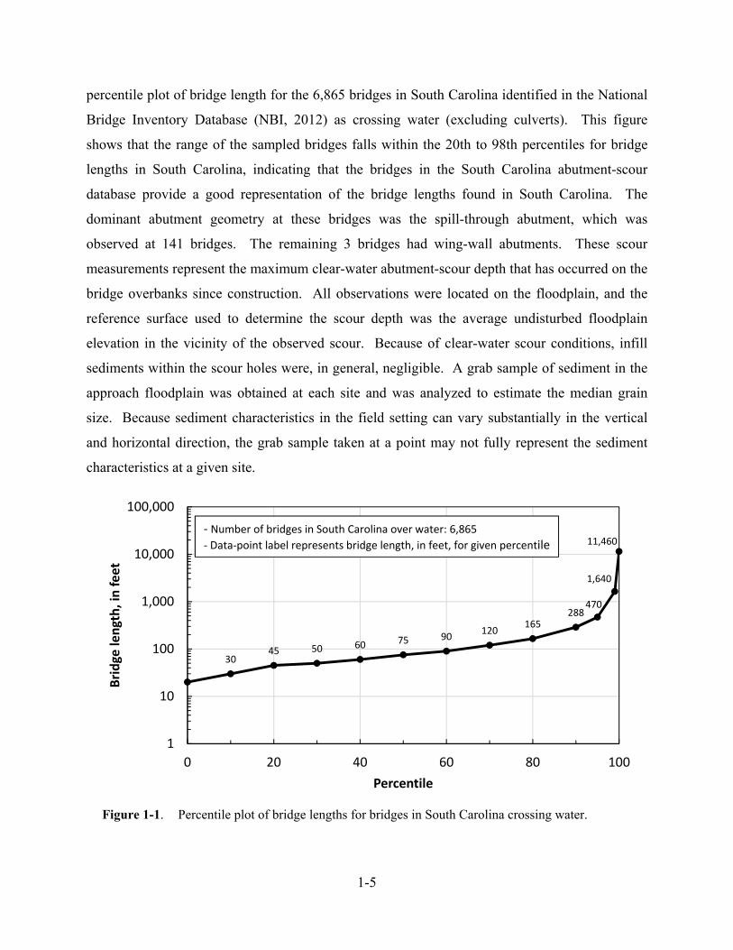
1-5
percentile plot of bridge length for the 6,865 bridges in South Carolina identified in the National
Bridge Inventory Database (NBI, 2012) as crossing water (excluding culverts). This figure
shows that the range of the sampled bridges falls within the 20th to 98th percentiles for bridge
lengths in South Carolina, indicating that the bridges in the South Carolina abutment-scour
database provide a good representation of the bridge lengths found in South Carolina. The
dominant abutment geometry at these bridges was the spill-through abutment, which was
observed at 141 bridges. The remaining 3 bridges had wing-wall abutments. These scour
measurements represent the maximum clear-water abutment-scour depth that has occurred on the
bridge overbanks since construction. All observations were located on the floodplain, and the
reference surface used to determine the scour depth was the average undisturbed floodplain
elevation in the vicinity of the observed scour. Because of clear-water scour conditions, infill
sediments within the scour holes were, in general, negligible. A grab sample of sediment in the
approach floodplain was obtained at each site and was analyzed to estimate the median grain
size. Because sediment characteristics in the field setting can vary substantially in the vertical
and horizontal direction, the grab sample taken at a point may not fully represent the sediment
characteristics at a given site.
Figure 1-1. Percentile plot of bridge lengths for bridges in South Carolina crossing water.
3045 50 60 75 90
120165
288470
1,640
11,460
1
10
100
1,000
10,000
100,000
0 20 40 60 80 100
Bridge length, in feet
Percentile
‐ Number of bridges in South Carolina over water: 6,865 ‐ Data‐point label represents bridge length, in feet, for given percentile
1-6
The South Carolina abutment-scour depths represent historical post-flood measurements that
were made during low-flow conditions, and the hydraulic conditions that created the scour are
not known. To gain insights into hydraulic conditions that may have created the observed scour,
numerical models were developed for each site using the one-dimensional step-backwater model,
WSPRO (Shearman, 1990). A review of streamgage records and the general flood history of
South Carolina indicated that 127 of the 144 bridges in the study likely had experienced flows
equaling or exceeding 70 percent of the 100-year flow magnitude (Benedict, 2003). Therefore,
the 100-year flow was assumed to be representative of a common flow that may have occurred at
all sites and was used in the WSPRO model for all of the bridges. All hydraulic variables
associated with the South Carolina data were derived from the WSPRO model and should be
viewed as approximate rather than measured data. The approximated hydraulic data will
introduce error into predicted scour computations, making the comparison of predicted and
observed abutment scour less than ideal. However, the large number of field observations (209)
in the database will allow trends to be assessed, providing insights into the strengths and
weaknesses of a particular equation.
The data collected in South Carolina have been grouped into two databases based on regional
location within the State. One database contains data collected in the Piedmont Physiographic
Province, and the other contains data collected in the Coastal Plain Physiographic Province.
(Sites in the Coastal Plain were not tidally influenced.) This division is justified due to the
distinct regional characteristics of the Piedmont and Coastal Plain Provinces. The Piedmont
generally has cohesive soils, moderate stream gradients with well-defined channels, relatively
narrow floodplains, and relatively short flood-flow durations. Setback abutments are common in
the Piedmont region, and figure 1-2 shows a typical bridge cross section for such sites, defining
the regions of clear-water scour on the bridge overbanks. Figure 1-3 shows a typical bridge plan
and profile for setback abutments. (Note: Relatively small piers are assumed to have negligible
influence on abutment-scour depth and are not shown in the bridge cross sections for figures 1-3
through 1-5. Findings from Benedict (2003) and Ettema et al. (2010) support this assumption.)
In contrast, the Coastal Plain generally has sandy soils, low gradient streams, relatively wide
floodplains, and relatively long flood-flow durations. While rivers with large drainage areas
typically have well-defined channels, many Coastal Plain streams are characterized by small,
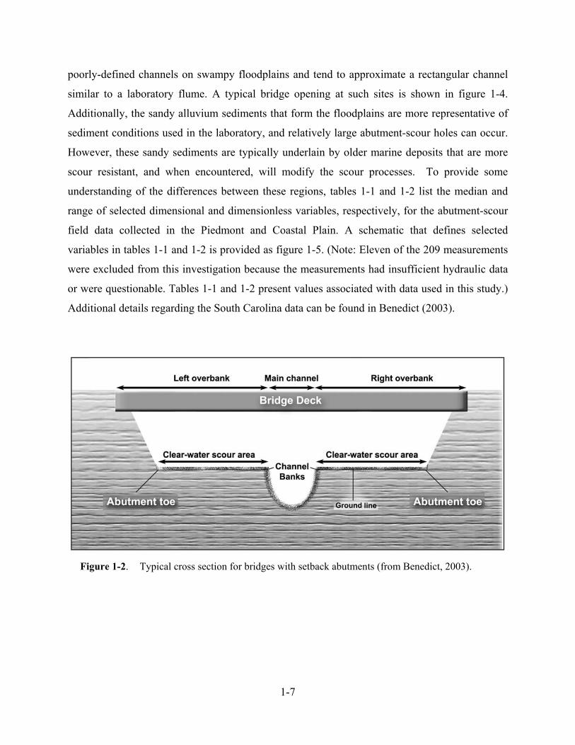
1-7
poorly-defined channels on swampy floodplains and tend to approximate a rectangular channel
similar to a laboratory flume. A typical bridge opening at such sites is shown in figure 1-4.
Additionally, the sandy alluvium sediments that form the floodplains are more representative of
sediment conditions used in the laboratory, and relatively large abutment-scour holes can occur.
However, these sandy sediments are typically underlain by older marine deposits that are more
scour resistant, and when encountered, will modify the scour processes. To provide some
understanding of the differences between these regions, tables 1-1 and 1-2 list the median and
range of selected dimensional and dimensionless variables, respectively, for the abutment-scour
field data collected in the Piedmont and Coastal Plain. A schematic that defines selected
variables in tables 1-1 and 1-2 is provided as figure 1-5. (Note: Eleven of the 209 measurements
were excluded from this investigation because the measurements had insufficient hydraulic data
or were questionable. Tables 1-1 and 1-2 present values associated with data used in this study.)
Additional details regarding the South Carolina data can be found in Benedict (2003).
Figure 1-2. Typical cross section for bridges with setback abutments (from Benedict, 2003).
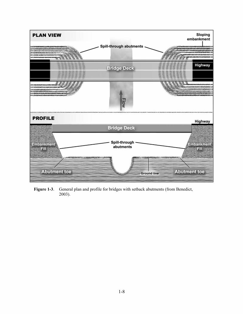
1-8
Figure 1-3. General plan and profile for bridges with setback abutments (from Benedict, 2003).
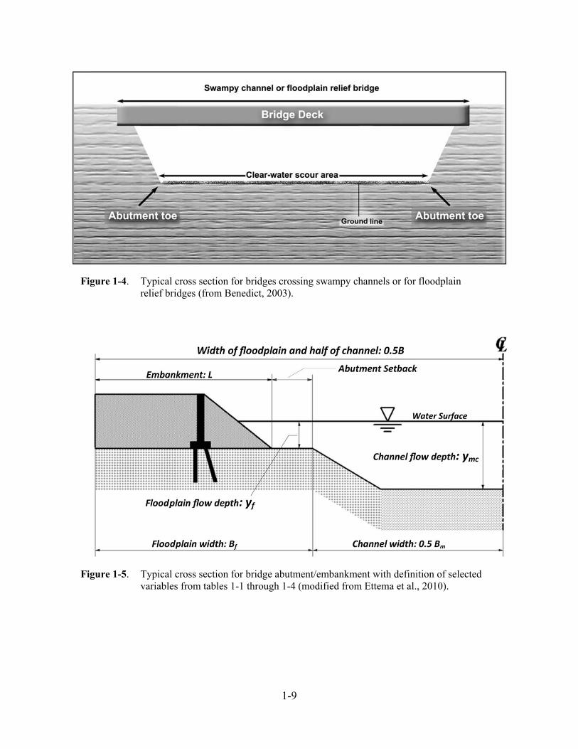
1-9
Figure 1-4. Typical cross section for bridges crossing swampy channels or for floodplain relief bridges (from Benedict, 2003).
Figure 1-5. Typical cross section for bridge abutment/embankment with definition of selected variables from tables 1-1 through 1-4 (modified from Ettema et al., 2010).
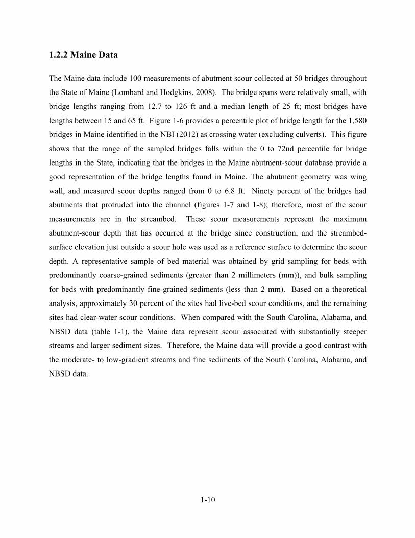
1-10
1.2.2 Maine Data
The Maine data include 100 measurements of abutment scour collected at 50 bridges throughout
the State of Maine (Lombard and Hodgkins, 2008). The bridge spans were relatively small, with
bridge lengths ranging from 12.7 to 126 ft and a median length of 25 ft; most bridges have
lengths between 15 and 65 ft. Figure 1-6 provides a percentile plot of bridge length for the 1,580
bridges in Maine identified in the NBI (2012) as crossing water (excluding culverts). This figure
shows that the range of the sampled bridges falls within the 0 to 72nd percentile for bridge
lengths in the State, indicating that the bridges in the Maine abutment-scour database provide a
good representation of the bridge lengths found in Maine. The abutment geometry was wing
wall, and measured scour depths ranged from 0 to 6.8 ft. Ninety percent of the bridges had
abutments that protruded into the channel (figures 1-7 and 1-8); therefore, most of the scour
measurements are in the streambed. These scour measurements represent the maximum
abutment-scour depth that has occurred at the bridge since construction, and the streambed-
surface elevation just outside a scour hole was used as a reference surface to determine the scour
depth. A representative sample of bed material was obtained by grid sampling for beds with
predominantly coarse-grained sediments (greater than 2 millimeters (mm)), and bulk sampling
for beds with predominantly fine-grained sediments (less than 2 mm). Based on a theoretical
analysis, approximately 30 percent of the sites had live-bed scour conditions, and the remaining
sites had clear-water scour conditions. When compared with the South Carolina, Alabama, and
NBSD data (table 1-1), the Maine data represent scour associated with substantially steeper
streams and larger sediment sizes. Therefore, the Maine data will provide a good contrast with
the moderate- to low-gradient streams and fine sediments of the South Carolina, Alabama, and
NBSD data.
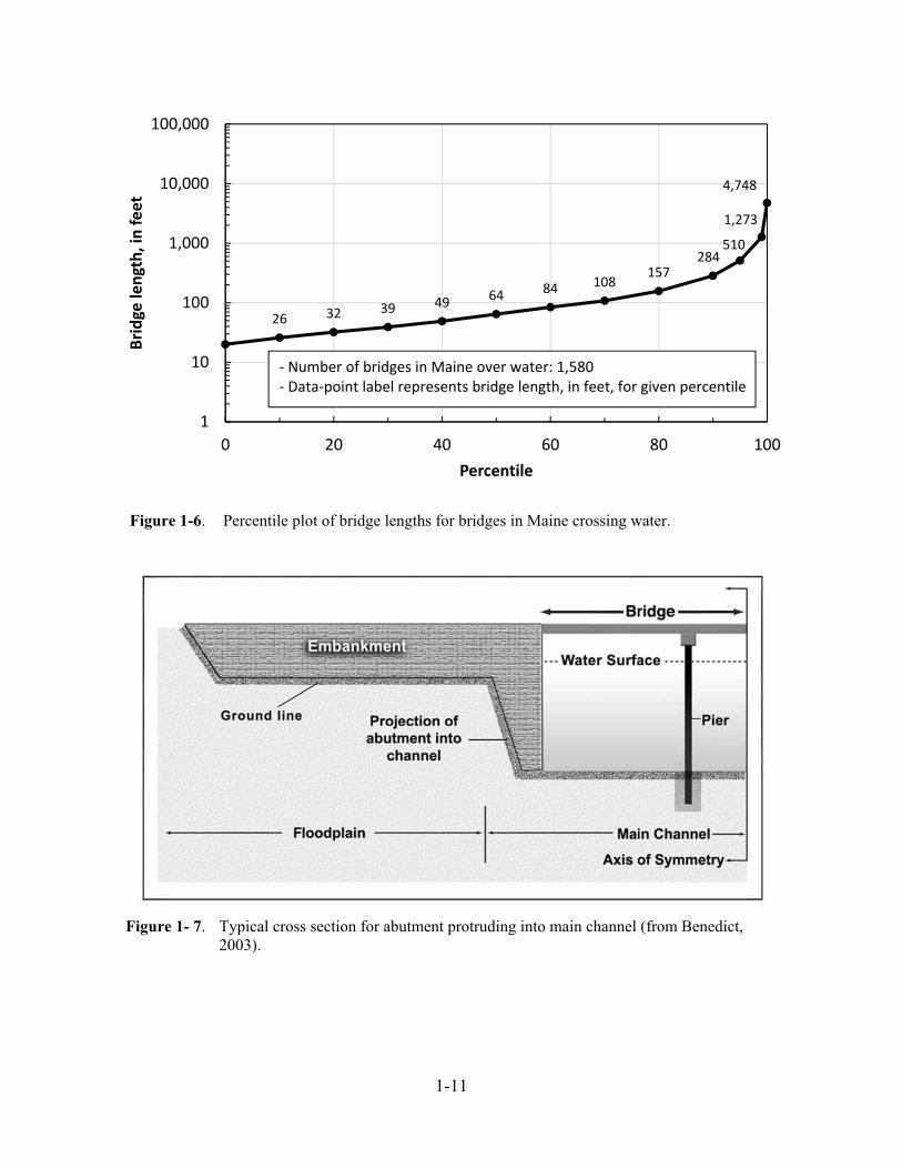
1-11
Figure 1-6. Percentile plot of bridge lengths for bridges in Maine crossing water.
Figure 1- 7. Typical cross section for abutment protruding into main channel (from Benedict, 2003).
26 32 39 49 64 84 108157
284510
1,273
4,748
1
10
100
1,000
10,000
100,000
0 20 40 60 80 100
Bridge length, in feet
Percentile
‐ Number of bridges in Maine over water: 1,580‐ Data‐point label represents bridge length, in feet, for given percentile
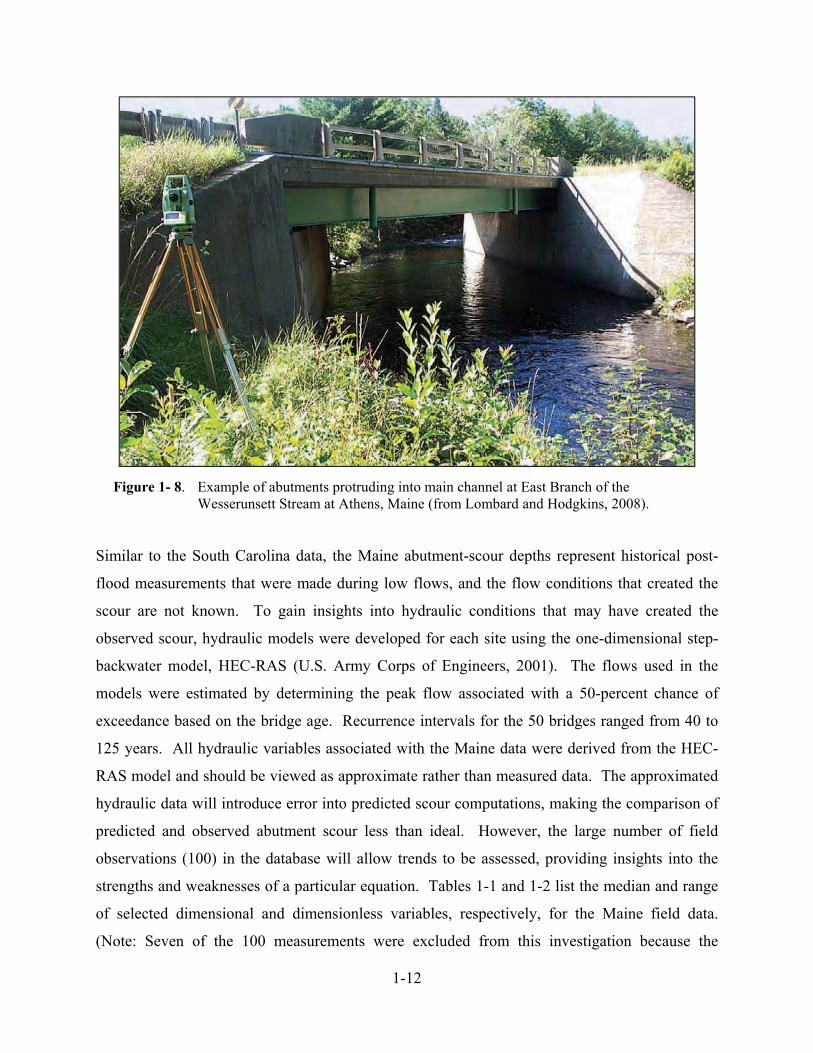
1-12
Figure 1- 8. Example of abutments protruding into main channel at East Branch of the Wesserunsett Stream at Athens, Maine (from Lombard and Hodgkins, 2008).
Similar to the South Carolina data, the Maine abutment-scour depths represent historical post-
flood measurements that were made during low flows, and the flow conditions that created the
scour are not known. To gain insights into hydraulic conditions that may have created the
observed scour, hydraulic models were developed for each site using the one-dimensional step-
backwater model, HEC-RAS (U.S. Army Corps of Engineers, 2001). The flows used in the
models were estimated by determining the peak flow associated with a 50-percent chance of
exceedance based on the bridge age. Recurrence intervals for the 50 bridges ranged from 40 to
125 years. All hydraulic variables associated with the Maine data were derived from the HEC-
RAS model and should be viewed as approximate rather than measured data. The approximated
hydraulic data will introduce error into predicted scour computations, making the comparison of
predicted and observed abutment scour less than ideal. However, the large number of field
observations (100) in the database will allow trends to be assessed, providing insights into the
strengths and weaknesses of a particular equation. Tables 1-1 and 1-2 list the median and range
of selected dimensional and dimensionless variables, respectively, for the Maine field data.
(Note: Seven of the 100 measurements were excluded from this investigation because the
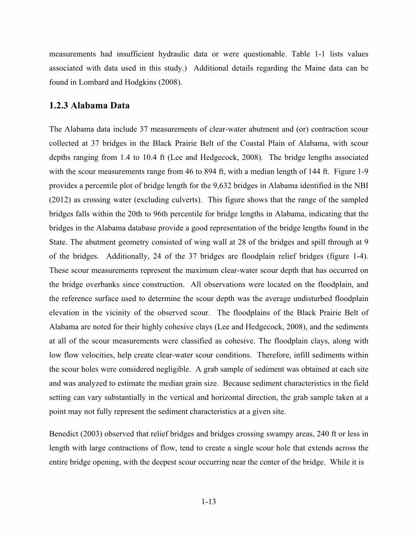
1-13
measurements had insufficient hydraulic data or were questionable. Table 1-1 lists values
associated with data used in this study.) Additional details regarding the Maine data can be
found in Lombard and Hodgkins (2008).
1.2.3 Alabama Data
The Alabama data include 37 measurements of clear-water abutment and (or) contraction scour
collected at 37 bridges in the Black Prairie Belt of the Coastal Plain of Alabama, with scour
depths ranging from 1.4 to 10.4 ft (Lee and Hedgecock, 2008). The bridge lengths associated
with the scour measurements range from 46 to 894 ft, with a median length of 144 ft. Figure 1-9
provides a percentile plot of bridge length for the 9,632 bridges in Alabama identified in the NBI
(2012) as crossing water (excluding culverts). This figure shows that the range of the sampled
bridges falls within the 20th to 96th percentile for bridge lengths in Alabama, indicating that the
bridges in the Alabama database provide a good representation of the bridge lengths found in the
State. The abutment geometry consisted of wing wall at 28 of the bridges and spill through at 9
of the bridges. Additionally, 24 of the 37 bridges are floodplain relief bridges (figure 1-4).
These scour measurements represent the maximum clear-water scour depth that has occurred on
the bridge overbanks since construction. All observations were located on the floodplain, and
the reference surface used to determine the scour depth was the average undisturbed floodplain
elevation in the vicinity of the observed scour. The floodplains of the Black Prairie Belt of
Alabama are noted for their highly cohesive clays (Lee and Hedgecock, 2008), and the sediments
at all of the scour measurements were classified as cohesive. The floodplain clays, along with
low flow velocities, help create clear-water scour conditions. Therefore, infill sediments within
the scour holes were considered negligible. A grab sample of sediment was obtained at each site
and was analyzed to estimate the median grain size. Because sediment characteristics in the field
setting can vary substantially in the vertical and horizontal direction, the grab sample taken at a
point may not fully represent the sediment characteristics at a given site.
Benedict (2003) observed that relief bridges and bridges crossing swampy areas, 240 ft or less in
length with large contractions of flow, tend to create a single scour hole that extends across the
entire bridge opening, with the deepest scour occurring near the center of the bridge. While it is
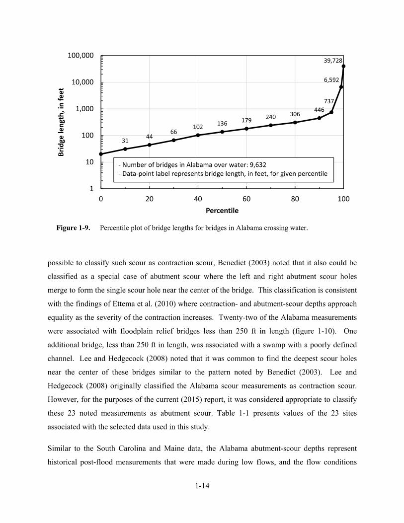
1-14
Figure 1-9. Percentile plot of bridge lengths for bridges in Alabama crossing water.
possible to classify such scour as contraction scour, Benedict (2003) noted that it also could be
classified as a special case of abutment scour where the left and right abutment scour holes
merge to form the single scour hole near the center of the bridge. This classification is consistent
with the findings of Ettema et al. (2010) where contraction- and abutment-scour depths approach
equality as the severity of the contraction increases. Twenty-two of the Alabama measurements
were associated with floodplain relief bridges less than 250 ft in length (figure 1-10). One
additional bridge, less than 250 ft in length, was associated with a swamp with a poorly defined
channel. Lee and Hedgecock (2008) noted that it was common to find the deepest scour holes
near the center of these bridges similar to the pattern noted by Benedict (2003). Lee and
Hedgecock (2008) originally classified the Alabama scour measurements as contraction scour.
However, for the purposes of the current (2015) report, it was considered appropriate to classify
these 23 noted measurements as abutment scour. Table 1-1 presents values of the 23 sites
associated with the selected data used in this study.
Similar to the South Carolina and Maine data, the Alabama abutment-scour depths represent
historical post-flood measurements that were made during low flows, and the flow conditions
3144
66102
136 179240 306
446
737
6,592
39,728
1
10
100
1,000
10,000
100,000
0 20 40 60 80 100
Bridge length, in feet
Percentile
‐ Number of bridges in Alabama over water: 9,632‐ Data‐point label represents bridge length, in feet, for given percentile
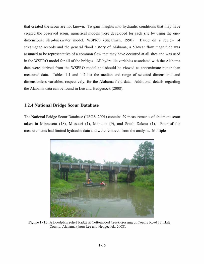
1-15
that created the scour are not known. To gain insights into hydraulic conditions that may have
created the observed scour, numerical models were developed for each site by using the one-
dimensional step-backwater model, WSPRO (Shearman, 1990). Based on a review of
streamgage records and the general flood history of Alabama, a 50-year flow magnitude was
assumed to be representative of a common flow that may have occurred at all sites and was used
in the WSPRO model for all of the bridges. All hydraulic variables associated with the Alabama
data were derived from the WSPRO model and should be viewed as approximate rather than
measured data. Tables 1-1 and 1-2 list the median and range of selected dimensional and
dimensionless variables, respectively, for the Alabama field data. Additional details regarding
the Alabama data can be found in Lee and Hedgecock (2008).
1.2.4 National Bridge Scour Database
The National Bridge Scour Database (USGS, 2001) contains 29 measurements of abutment scour
taken in Minnesota (18), Missouri (1), Montana (9), and South Dakota (1). Four of the
measurements had limited hydraulic data and were removed from the analysis. Multiple
Figure 1- 10. A floodplain relief bridge at Cottonwood Creek crossing of County Road 12, Hale County, Alabama (from Lee and Hedgecock, 2008).
1-16
measurements at several small bridges were considered redundant, and 2 measurements were
removed. Additionally, 16 of the measurements were associated with time-series measurements
or concurrent measurements at the upstream and downstream bridge faces. At these sites, the
largest scour measurement was included in the investigation, with 8 smaller measurements
excluded. The 15 measurements included in the NCHRP 24-20(2) analysis included 8
measurements in Minnesota, 6 in Montana, and 1 in South Dakota. The scour measurements at
the Minnesota sites were obtained during flood conditions along with concurrent flow
measurement data at or near the sites. The other measurements are post-flood measurements
(similar to those in the South Carolina, Maine, and Alabama data) with estimates of the flow
conditions from indirect flow measurements or gage data. For the 15 measurements included in
the NCHRP 24-20(2) analysis, bridge lengths ranged from 88 to 450 ft with a median length of
121 ft, and abutment-scour depths ranged from 0 to 18 ft. The abutment geometry at 13 of the
measurements was the spill-through abutment, with the remaining measurements associated with
wing-wall abutments.
While all of the NBSD data have supporting flow measurements, one-dimensional flow models
(HEC-RAS or WSPRO), with the associated flow data, were required to estimate the hydraulic
properties at the approach and bridge sections. Some of the hydraulic data required for
application to the scour prediction methods were not published in the NBSD, and these data were
obtained for the current investigation (2015) by referring to the unpublished models. Seven of
the scour measurements are associated with meandering streams that are challenging to model
with a one-dimensional flow model. The one-dimensional flow models associated with the
NBSD data were reviewed and in some cases modified to better represent the unconstricted
approach section. The models provide estimates of the hydraulic conditions that likely created
the scour, but the site complexities and limitations of one-dimensional models will likely
introduce some error in estimates and the hydraulic data should be viewed as approximate rather
than measured data. Tables 1-1 and 1-2 list the median and range of selected dimensional and
dimensionless variables, respectively, for the NBSD field data. Additional details associated
with the data can be found at the NBSD Web page (http://water.usgs.gov/
osw/techniques/bs/BSDMS/) as well as in Wagner et al. (2006).

1-17
Table 1-1. Range of selected variables for abutment-scour measurements in the South Carolina, Maine, Alabama, and National Bridge Scour Databases. (Refer to figure 1-5 for schematic showing selected variable definitions.) [miles2, square miles; ft, feet; ft/s, feet per second; mm, millimeters]
Range value
Drainage area
(miles2)
Channel slope (ft/ft)
Average abutment approach velocity
(ft/s)
Average abutment approach depth (y1)
(ft)
Embankment length (L)
blocking flow (ft)
Median grain size
(mm)
Observed abutment-
scour depth
(ft) South Carolina Piedmont (92 observations)
Minimum 10.7 0.00015 0.17 2.19 18.4 0.003 0.0
Median 76 0.00120 0.96 5.90 268 0.029 1.2
Maximum 1,620 0.00240 3.57 15.60 1,669 0.447 18.0
South Carolina Coastal Plain (106 observations)
Minimum 6.1 0.00007 0.05 2.00 86.7 0.005 0.0
Median 120 0.00054 0.48 4.91 610 0.179 7.0
Maximum 8,830 0.00240 0.96 16.04 7,440 0.782 23.6
Maine (93 observations)
Minimum 4.1 0.00041 0.18 1.11 0.0 0.25 0.0
Median 20.1 0.00275 1.04 7.06 40.1 45 0.0
Maximum 95.1 0.04446 5.62 15.25 808 109 6.8
Alabama (23 observations)
Minimum 10.0 0.00040 0.18 3.21 43.0 0.001 1.4
Median 80.2 0.00080 0.62 5.00 400 0.009 4.7
Maximum 607 0.00160 1.31 9.34 1,141 0.170 10.4
National Bridge Scour Database (15 observations)
Minimum 836 0.00050 0.49 3.95 15.0 0.001 0.0
Median 970 0.00060 0.71 8.81 560 0.150 4.5
Maximum 16,010 0.00060 3.37 36.56 3,522 35 18.0
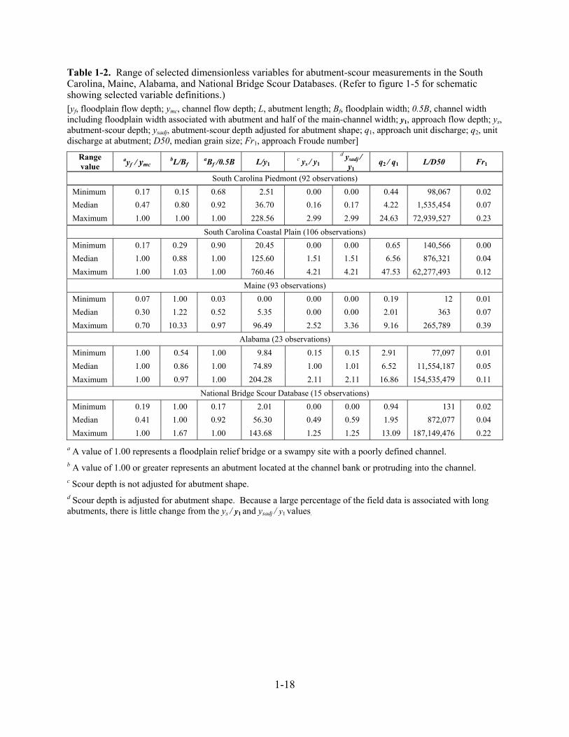
1-18
Table 1-2. Range of selected dimensionless variables for abutment-scour measurements in the South Carolina, Maine, Alabama, and National Bridge Scour Databases. (Refer to figure 1-5 for schematic showing selected variable definitions.) [yf, floodplain flow depth; ymc, channel flow depth; L, abutment length; Bf, floodplain width; 0.5B, channel width including floodplain width associated with abutment and half of the main-channel width; y1, approach flow depth; ys, abutment-scour depth; ysadj, abutment-scour depth adjusted for abutment shape; q1, approach unit discharge; q2, unit discharge at abutment; D50, median grain size; Fr1, approach Froude number]
Range value
ayf / ymc bL/Bf
aBf /0.5B L/y1 c ys / y1
d ysadj / y1
q2 / q1 L/D50 Fr1
South Carolina Piedmont (92 observations)
Minimum 0.17 0.15 0.68 2.51 0.00 0.00 0.44 98,067 0.02
Median 0.47 0.80 0.92 36.70 0.16 0.17 4.22 1,535,454 0.07
Maximum 1.00 1.00 1.00 228.56 2.99 2.99 24.63 72,939,527 0.23
South Carolina Coastal Plain (106 observations)
Minimum 0.17 0.29 0.90 20.45 0.00 0.00 0.65 140,566 0.00
Median 1.00 0.88 1.00 125.60 1.51 1.51 6.56 876,321 0.04
Maximum 1.00 1.03 1.00 760.46 4.21 4.21 47.53 62,277,493 0.12
Maine (93 observations)
Minimum 0.07 1.00 0.03 0.00 0.00 0.00 0.19 12 0.01
Median 0.30 1.22 0.52 5.35 0.00 0.00 2.01 363 0.07
Maximum 0.70 10.33 0.97 96.49 2.52 3.36 9.16 265,789 0.39
Alabama (23 observations)
Minimum 1.00 0.54 1.00 9.84 0.15 0.15 2.91 77,097 0.01
Median 1.00 0.86 1.00 74.89 1.00 1.01 6.52 11,554,187 0.05
Maximum 1.00 0.97 1.00 204.28 2.11 2.11 16.86 154,535,479 0.11
National Bridge Scour Database (15 observations)
Minimum 0.19 1.00 0.17 2.01 0.00 0.00 0.94 131 0.02
Median 0.41 1.00 0.92 56.30 0.49 0.59 1.95 872,077 0.04
Maximum 1.00 1.67 1.00 143.68 1.25 1.25 13.09 187,149,476 0.22
a A value of 1.00 represents a floodplain relief bridge or a swampy site with a poorly defined channel. b A value of 1.00 or greater represents an abutment located at the channel bank or protruding into the channel. c Scour depth is not adjusted for abutment shape. d Scour depth is adjusted for abutment shape. Because a large percentage of the field data is associated with long abutments, there is little change from the ys / y1 and ysadj / y1 values.
1-19
1.2.5 Limitations
Laboratory investigations have been essential in advancing the understanding of abutment scour
and undoubtedly will continue to play a prominent role in future investigations. However, field
conditions will often differ from the idealized conditions of the laboratory, and it is important to
understand some of these differences. Laboratory models typically consist of simple river plans
that include uniform channel geometry, straight approach channels, uniform floodplain and
channel roughness, uniform non-cohesive sediments, approach flow velocities near threshold
conditions, and constant flow of sufficient duration to create equilibrium scour depths (Melville
and Coleman, 2000). These characteristics rarely exist concurrently in the field, and the
equilibrium abutment-scour depth associated with the laboratory studies is likely unattainable at
most field sites. As will be shown later in this chapter, the upper bound of the relative scour
depth (scour depth divided by approach flow depth) for the laboratory data is about 11 for rigid
abutment/embankment models and about 4 for erodible abutment/embankment models as used in
the NCHRP 24-20 investigations. In comparison, the maximum relative scour depth is 4.2 for
the USGS field data. The upper bound within the USGS field data has some confirmation from
the large abutment-scour measurement at the Interstate 70 (I-70) crossing of the Missouri River
(Parola et al. 1998). The I-70 abutment scour was caused by the 1993 flood with high-flow
durations lasting nearly 7 days. The scour was strongly influenced by an upstream levee breach
in close proximity to the abutment, and the largest scour depth (56 ft) was located just
downstream from the breach. As flows moved around the embankment and into the bridge
opening, the deepest scour depth at the bridge was 30 ft. These scour depths were not created by
the typical flow patterns associated with abutment scour, but rather by adverse conditions that
tend to promote large scour depths. The I-70 scour depths are presented here for perspective.
The relative abutment-scour depth for the 56-ft deep measurement is 4.0 indicating that the upper
bound of abutment scour in the USGS data is not unreasonable for the field, even under severe
flood conditions, such as the I-70 measurements.
The NCHRP 24-20 investigation demonstrates how laboratory models with erodible
embankments and abutment substructures, comparable to conditions often found in the field, will
tend to reduce the magnitude of abutment scour in comparison to laboratory models with rigid
abutments/embankments that have vertical-wall substructures that extend fully into the bed
1-20
sediments. It is of interest that the largest relative scour depth for the NCHRP 24-20 data, about
4, conforms well to that of the field, about 4.2. The similarity in the largest relative scour depths
could indicate that erodible abutment substructures produced the smaller scour depths in the
USGS field data, similar to those of the NCHRP 24-20 data. While this may contribute in some
measure to this pattern, the evidence indicates that abutments/embankments associated with the
USGS field data largely remained intact; therefore, the smaller relative scour depths cannot be
attributed solely to this type of scour process. While many factors likely contribute to the
smaller relative abutment-scour depths in the field data, non-uniform sediments, short flow
durations, and approach flow velocities below critical-velocity conditions are thought to be
prominent reasons for the discrepancies between the laboratory data associated with rigid
abutment models and the field data.
Sediment characteristics can play a prominent role in preventing the attainment of equilibrium
abutment-scour depths in the field. Sediments in the field are non-uniform in grain size and
often have varying degrees of cohesion. This is particularly the case for floodplain sediments
where clear-water abutment scour occurs at setback abutments. Additionally, natural streams
with alluvium floodplain sediments often have subsurface strata that are more resistant to scour
than the surface sediments. In the South Carolina data, it was common for abutment-scour holes,
exceeding approximately 5 ft in depth, to cut down to a scour-resistant layer that likely impeded
scour (Benedict, 2003). Of the South Carolina abutment-scour measurements, 124 resulted in
scour depths less than 5 ft. For these smaller scour depths, only one measurement had a
subsurface scour-resistant layer at the bottom of the scour hole that was distinctly different from
the surface sediments. In contrast, of the 85 abutment-scour measurements in South Carolina
that had scour depths exceeding 5 ft, 48 measurements had a subsurface scour-resistant sediment
layer at the bottom of the scour hole. Similarly, Parola et al. (1998) note that the 56-ft-deep
abutment-scour hole at the I-70 crossing of the Missouri River likely was limited by a subsurface
layer of relatively resistant material. These sediment characteristics, commonly found in the
field, will tend to reduce the magnitude of relative scour in comparison to the uniform non-
cohesive sediments of the laboratory, and these sediment characteristics are thought to be a
prominent reason for the smaller relative scour depths in the field.
1-21
Another factor that could limit the attainment of equilibrium abutment-scour depths in the field
comparable to those of the laboratory is insufficient flow duration. Flow durations must often
last for days in laboratory experiments in order to achieve equilibrium abutment-scour depths
(Sturm, 2004). In contrast, small to moderate drainage areas, commonly associated with many
bridges, will have peak-flow durations substantially smaller than those of the laboratory, thus
limiting the potential to attain equilibrium abutment-scour depths. This is particularly the case
for clear-water abutment scour on the floodplain, because it takes longer flow durations to attain
equilibrium clear-water scour depths (Melville and Coleman, 2000).
The largest potential for abutment-scour depth generally occurs when approach flow velocities
are near the sediment critical velocity (Melville and Coleman, 2000), which is the threshold
velocity that transitions from clear-water to live-bed scour conditions. Laboratory experiments
are often conducted near threshold velocity in order to assess the worst-case conditions for
abutment scour. As approach flow velocities decrease below threshold velocities, scour depth
decreases (Melville and Coleman, 2000). As will be shown later in report section 1.4.1, flow
velocities on the approach floodplain are often below threshold velocities and will likely
contribute to the smaller relative-scour depths observed in the field. Because abutment-scour
field data tend to have relative scour depths smaller than the laboratory, it is logical to assume
that laboratory-derived equations applied to field data should consistently overpredict the field
measurements. If underprediction frequently occurs, additional consideration should be given to
assess why this is the case.
All of the hydraulic properties used in this investigation are based on one-dimensional flow
models. As such, they must be viewed as approximate rather than measured data, and such data
will likely introduce error in the predicted scour. The South Carolina, Alabama, and Maine
investigations assumed various flow conditions for use in the hydraulic models. Based on a
review of historical flow records, the South Carolina and Alabama studies assumed that the 100-
year and 50-year peak flows, respectively, would represent approximate flow conditions that
created the measured scour. For the Maine investigation, the peak flow associated with a 50-
percent chance of exceedance based on the bridge age was used to represent the hydraulic
conditions that may have created the scour. It is likely that these flow magnitudes will provide
overestimates of hydraulic conditions, especially for the South Carolina data. The NCHRP 24-

1-22
20 and 24-15(2) methods require estimates of the flow velocity at the abutment. One-
dimensional flow models often do not simulate well the increased flow velocities at large flow
contractions at an abutment and, therefore, will tend to underestimate this value. Underestimates
of the velocity at the abutment will tend to produce underestimates of abutment-scour depth. To
compensate for this limitation in one-dimensional flow models, the NCHRP 24-20 and 24-15(2)
methods use algorithms, described later in the report, that provide conservative estimates of the
flow velocity at the abutment. These algorithms likely perform well at sites with a well-defined
channel. However, at sites with poorly defined channels, such as a swamp or floodplain relief
bridge, the algorithms may underestimate the increased flow velocity at the abutment.
The uncertainty and limitations associated with the USGS field data, as noted above, will
introduce some error into any analysis in which these data are used. Therefore, relations in the
field data and comparisons of predicted and measured field data will generally have more scatter
than that associated with laboratory data. While the limitations of the USGS field data are
acknowledged, it is currently (2015) the best available set of field data for the evaluation of
abutment-scour prediction equations. The error and limitations make these data less than ideal;
however, the large number of field observations used in the analysis (329) and the wide range of
regional characteristics associated with the data allow trends for selected scour prediction
methods to be assessed. Such an assessment will provide insights into the strengths, weaknesses,
and limitations of a particular scour prediction method.
1.3 Laboratory Data
The harsh and uncontrolled environment of the field makes it challenging to measure abutment
scour and the associated hydraulic characteristics creating the scour. In contrast, the controlled
environment of the laboratory allows for more accurate measurement of these values. While the
objective of this investigation is to evaluate the performance of the NCHRP 24-15(2) and
NCHRP 24-20 methods with field data, the use of the more precise laboratory data can help
confirm the trends observed in the field data assessment. Selected data from Palaviccini (1993)
and Sturm (2004) were compiled and used to compare with the dimensionless trends of the
laboratory data for NCHRP 24-15(2) and NCHRP 24-20. Additionally, these data were applied
to the NCHRP 24-15(2) and NCHRP 24-20 equations to assist in evaluating the performance of
1-23
these equations. The Palaviccini (1993) data consist of 404 measurements of live-bed and clear-
water abutment scour compiled from selected investigations prior to 1990. The measurements
were collected in rectangular flumes and included 57 spill-through, 56 wing-wall, 246 vertical-
wall, and 45 other types of abutments. The Palaviccini (1993) data associated with spill-through,
wing-wall, and vertical-wall abutments were used in this investigation. The Sturm (2004) data
consist of 74 measurements of clear-water abutment scour collected in compound channels, more
closely reflecting the laboratory conditions associated with the NCHRP 24-15(2) and NCHRP
24-20. These data represent longer abutment lengths than those associated with Palaviccini
(1993) and the NCHRP 24-15(2) and NCHRP 24-20 investigations and include spill-through and
vertical-wall abutments. Additionally, the Sturm (2004) data include point measurements of
velocity and depth at the approach floodplain, as well as measurements of the maximum velocity
and associated depth at the abutment. These data provide a means to determine the unit
discharges at the approach and bridge, which are the primary variables used in the NCHRP 24-20
method.
Some notable differences in the Palaviccini (1993) and Sturm (2004) data from the NCHRP 24-
15(2) and NCHRP 24-20 data include the following. The NCHRP 24-15(2) method was
originally developed for scour in cohesive sediments, but was expanded to include scour in non-
cohesive sediments (Briaud et al. 2009; 2011), as is described later in the report. The Palaviccini
(1993) and Sturm (2004) data represent scour in non-cohesive sediments, making it difficult to
assess the performance of the NCHRP 24-15(2) method for scour in cohesive sediments, but
useful for assessing equation performance in non-cohesive sediments. The NCHRP 24-20
laboratory investigation evaluated scour for various combinations of erodible and non-erodible
floodplains, embankments, and abutment substructures. In contrast, the other laboratory
investigations evaluated scour for solid-form (rigid) abutments typically having a vertical wall at
the abutment toe, similar to a sheet-pile skirt, extending into the bed. The erodible
abutment/embankment models will tend to reduce abutment-scour depth in contrast to the rigid
abutment/embankment models. The Palaviccini (1993) and Sturm (2004) data represent rigid
abutments/embankments, and some underprediction is likely when these data are applied to the
NCHRP 24-20 method. Tables 1-3 and 1-4 list the median and range of selected dimensional
and dimensionless variables, respectively, for the Palaviccini (1993) and Sturm (2004) data.
Figure 1-5 provides a schematic that defines selected variables in tables 1-3 and 1-4. Data
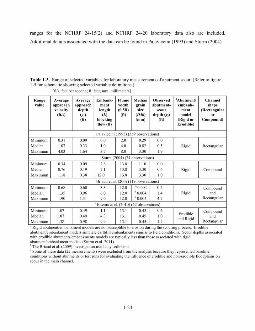
1-24
ranges for the NCHRP 24-15(2) and NCHRP 24-20 laboratory data also are included.
Additional details associated with the data can be found in Palaviccini (1993) and Sturm (2004).
Table 1-3. Range of selected variables for laboratory measurements of abutment scour. (Refer to figure 1-5 for schematic showing selected variable definitions.)
[ft/s, feet per second; ft, feet; mm, millimeters]
Range value
Average approach velocity
(ft/s)
Average approach
depth (y1) (ft)
Embank-ment
length (L)
blocking flow (ft)
Flume width (0.5B)
(ft)
Median grain size
(D50) (mm)
Observed abutment-
scour depth (ys)
(ft)
aAbutment/ embank-
ment model
(Rigid or Erodible)
Channel shape
(Rectangular or
Compound)
Palaviccini (1993) (359 observations)
Minimum 0.31 0.09 0.0 2.0 0.29 0.0 Rigid Rectangular Median 1.07 0.33 1.0 4.0 0.82 0.5
Maximum 4.03 1.64 3.7 8.0 3.30 1.9
Sturm (2004) (74 observations)
Minimum 0.34 0.09 2.6 13.8 1.10 0.0 Rigid Compound Median 0.76 0.19 7.1 13.8 3.30 0.6
Maximum 1.18 0.38 12.0 13.8 3.30 1.0
Briaud et al. (2009) (19 observations)
Minimum 0.68 0.60 3.3 12.0 b 0.004 0.2 Rigid
Compound and
Rectangular Median 1.35 0.96 6.0 12.0 b 0.004 1.4 Maximum 1.90 1.31 9.0 12.0 b 0.004 4.7
c Ettema et al. (2010) (62 observations)
Minimum 1.07 0.49 1.1 13.1 0.45 0.6 Erodible and Rigid
Compound and
Rectangular Median 1.07 0.49 4.3 13.1 0.45 1.0 Maximum 1.38 0.98 9.9 13.1 0.45 1.4
a Rigid abutment/embankment models are not susceptible to erosion during the scouring process. Erodible abutment/embankment models simulate earthfill embankments similar to field conditions. Scour depths associated with erodible abutments/embankments models are typically less than those associated with rigid abutment/embankment models (Sturm et al. 2011). b The Briaud et al. (2009) investigation used clay sediments. c Some of these data (22 measurements) were excluded from the analysis because they represented baseline conditions without abutments or test runs for evaluating the influence of erodible and non-erodible floodplains on scour in the main channel.
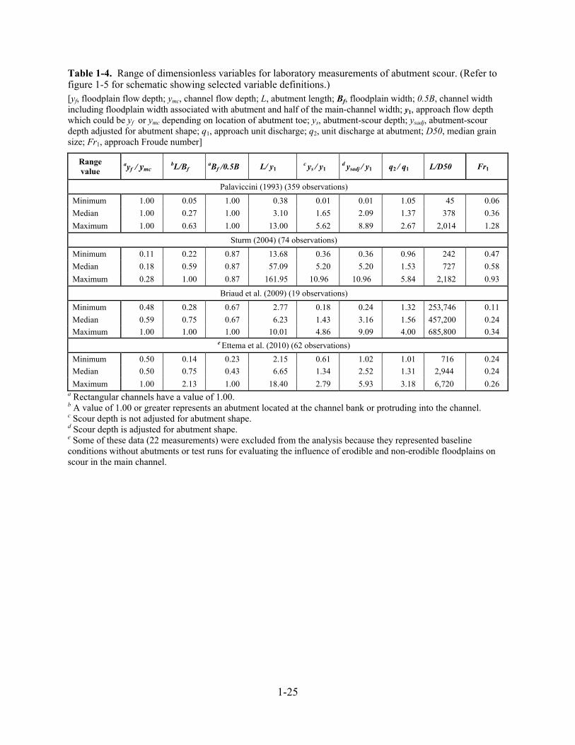
1-25
Table 1-4. Range of dimensionless variables for laboratory measurements of abutment scour. (Refer to figure 1-5 for schematic showing selected variable definitions.) [yf, floodplain flow depth; ymc, channel flow depth; L, abutment length; Bf, floodplain width; 0.5B, channel width including floodplain width associated with abutment and half of the main-channel width; y1, approach flow depth which could be yf or ymc depending on location of abutment toe; ys, abutment-scour depth; ysadj, abutment-scour depth adjusted for abutment shape; q1, approach unit discharge; q2, unit discharge at abutment; D50, median grain size; Fr1, approach Froude number]
Range value
ayf / ymc bL/Bf aBf /0.5B L/ y1 c ys / y1
d ysadj / y1 q2 / q1 L/D50 Fr1
Palaviccini (1993) (359 observations)
Minimum 1.00 0.05 1.00 0.38 0.01 0.01 1.05 45 0.06
Median 1.00 0.27 1.00 3.10 1.65 2.09 1.37 378 0.36
Maximum 1.00 0.63 1.00 13.00 5.62 8.89 2.67 2,014 1.28
Sturm (2004) (74 observations)
Minimum 0.11 0.22 0.87 13.68 0.36 0.36 0.96 242 0.47
Median 0.18 0.59 0.87 57.09 5.20 5.20 1.53 727 0.58
Maximum 0.28 1.00 0.87 161.95 10.96 10.96 5.84 2,182 0.93
Briaud et al. (2009) (19 observations)
Minimum 0.48 0.28 0.67 2.77 0.18 0.24 1.32 253,746 0.11
Median 0.59 0.75 0.67 6.23 1.43 3.16 1.56 457,200 0.24
Maximum 1.00 1.00 1.00 10.01 4.86 9.09 4.00 685,800 0.34 e Ettema et al. (2010) (62 observations)
Minimum 0.50 0.14 0.23 2.15 0.61 1.02 1.01 716 0.24
Median 0.50 0.75 0.43 6.65 1.34 2.52 1.31 2,944 0.24
Maximum 1.00 2.13 1.00 18.40 2.79 5.93 3.18 6,720 0.26 a Rectangular channels have a value of 1.00. b A value of 1.00 or greater represents an abutment located at the channel bank or protruding into the channel. c Scour depth is not adjusted for abutment shape. d Scour depth is adjusted for abutment shape. e Some of these data (22 measurements) were excluded from the analysis because they represented baseline conditions without abutments or test runs for evaluating the influence of erodible and non-erodible floodplains on scour in the main channel.
1-26
1.3.1 Adjustment for Abutment Shape
The following sections of this report will present some simple comparisons of the laboratory and
field data. When making such comparisons, it is useful to adjust the data to a common abutment
shape, and a brief description of this adjustment procedure follows. Abutment shape can have a
strong influence on abutment-scour depth, with blunt abutment shapes, such as vertical walls,
creating larger scour depths than streamlined shapes, such as spill-through abutments. As the
abutment length increases, the benefits of a streamlined shape diminish and scour depths
approach those of the blunt-faced abutments (Melville and Coleman, 2000). In order to review
and compare the relations in the laboratory data (table 1-3), it is necessary to convert scour
depths associated with various abutment shapes to a common reference shape. This conversion
is accomplished by dividing the measured scour depth by the associated abutment-shape factor
(table 1-5). To account for the change in the abutment-shape factor as abutment length
increases, Melville and Coleman (2000) recommend the following equations. By using equation
1-1, the laboratory data (table 1-3) were converted to a common reference shape prior to
investigating selected relations by dividing the measured scour depth by the associated abutment-
shape factor.
∗ , for L/y1 ≤ 10 (1-1a)
∗ 0.667 1 0.1 1 , for 10 < L/y1 < 25 (1-1b)
∗ 1 for L/y1 ≥ 25 (1-1c)
where
∗ is the abutment-shape factor adjusted for abutment length;
is the abutment-shape factor for shorter abutments (table 1-5);
L is the abutment length in ft; and
y1 is the approach flow depth in ft.
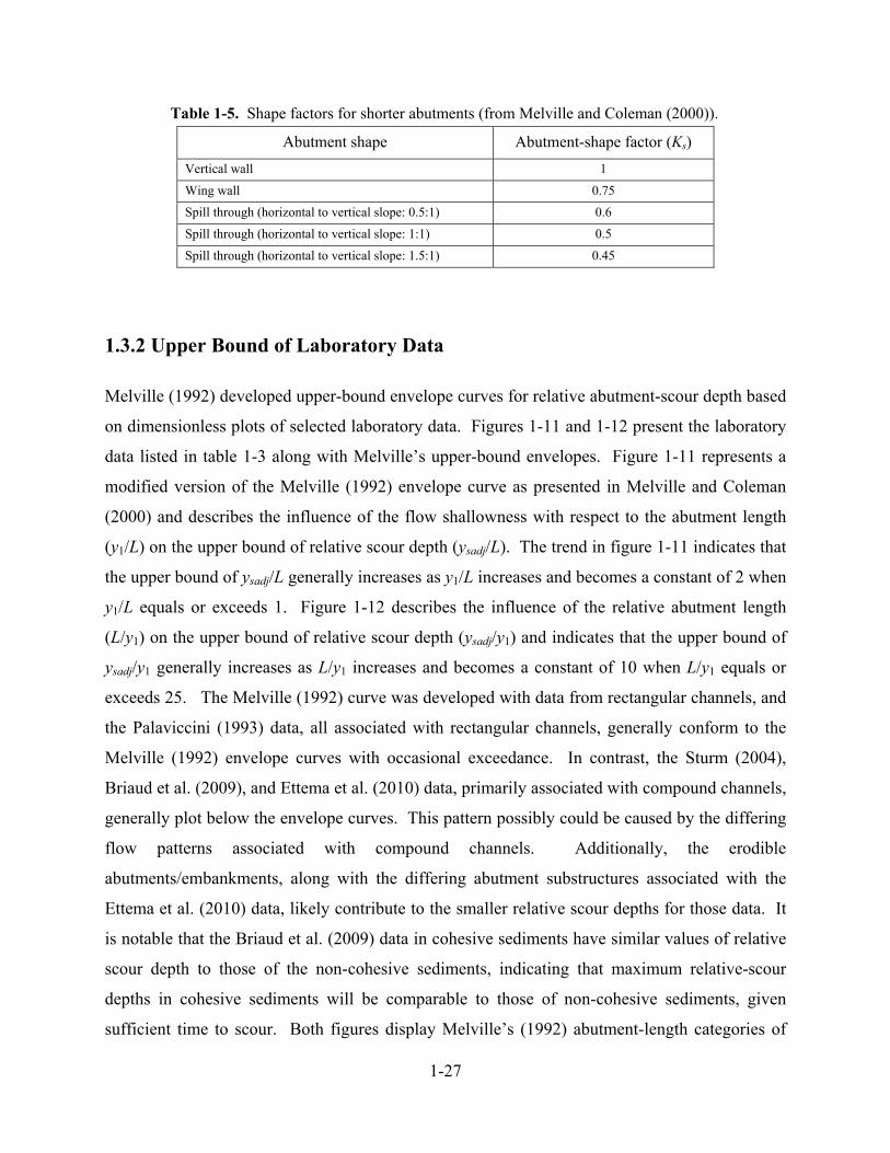
1-27
Table 1-5. Shape factors for shorter abutments (from Melville and Coleman (2000)).
Abutment shape Abutment-shape factor (Ks)
Vertical wall 1
Wing wall 0.75
Spill through (horizontal to vertical slope: 0.5:1) 0.6
Spill through (horizontal to vertical slope: 1:1) 0.5
Spill through (horizontal to vertical slope: 1.5:1) 0.45
1.3.2 Upper Bound of Laboratory Data
Melville (1992) developed upper-bound envelope curves for relative abutment-scour depth based
on dimensionless plots of selected laboratory data. Figures 1-11 and 1-12 present the laboratory
data listed in table 1-3 along with Melville’s upper-bound envelopes. Figure 1-11 represents a
modified version of the Melville (1992) envelope curve as presented in Melville and Coleman
(2000) and describes the influence of the flow shallowness with respect to the abutment length
(y1/L) on the upper bound of relative scour depth (ysadj/L). The trend in figure 1-11 indicates that
the upper bound of ysadj/L generally increases as y1/L increases and becomes a constant of 2 when
y1/L equals or exceeds 1. Figure 1-12 describes the influence of the relative abutment length
(L/y1) on the upper bound of relative scour depth (ysadj/y1) and indicates that the upper bound of
ysadj/y1 generally increases as L/y1 increases and becomes a constant of 10 when L/y1 equals or
exceeds 25. The Melville (1992) curve was developed with data from rectangular channels, and
the Palaviccini (1993) data, all associated with rectangular channels, generally conform to the
Melville (1992) envelope curves with occasional exceedance. In contrast, the Sturm (2004),
Briaud et al. (2009), and Ettema et al. (2010) data, primarily associated with compound channels,
generally plot below the envelope curves. This pattern possibly could be caused by the differing
flow patterns associated with compound channels. Additionally, the erodible
abutments/embankments, along with the differing abutment substructures associated with the
Ettema et al. (2010) data, likely contribute to the smaller relative scour depths for those data. It
is notable that the Briaud et al. (2009) data in cohesive sediments have similar values of relative
scour depth to those of the non-cohesive sediments, indicating that maximum relative-scour
depths in cohesive sediments will be comparable to those of non-cohesive sediments, given
sufficient time to scour. Both figures display Melville’s (1992) abutment-length categories of

1-28
short, intermediate, and long abutments, and indicate that the Palaviccini (1993) data consist of
short and intermediate abutments; the Briaud et al. (2009) and Ettema et al. (2010) data consist
of intermediate abutments; and the Sturm (2004) data consists primarily of long abutments with a
few intermediate abutments. The diversity of the Palaviccini (1993) and Sturm (2004) data with
respect to the Briaud et al. (2009) and Ettema et al. (2010) data indicates that applying these data
to the NCHRP 24-15(2) and NCHRP 24-20 methods will likely provide good insights to the
performance of those methods.
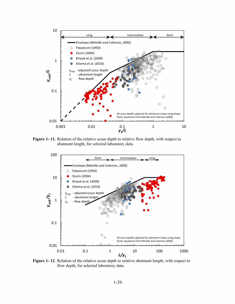
1-29
Figure 1- 11. Relation of the relative scour depth to relative flow depth, with respect to abutment length, for selected laboratory data.
Figure 1- 12. Relation of the relative scour depth to relative abutment length, with respect to flow depth, for selected laboratory data.
0.01
0.1
1
10
0.001 0.01 0.1 1 10
y sadj /L
y1/L
Envelope (Melville and Coleman, 2000)
PalavIccini (1993)
Sturm (2004)
Briaud et al. (2009)
Ettema et al. (2010)
All scour depths adjusted for abutment shape using shapefactor equations fromMelville and Coleman (2000).
Long Intermediate Short
ysadj ‐ adjusted scour depthL ‐ abutment lengthy1 ‐ flow depth
0.01
0.1
1
10
100
0.01 0.1 1 10 100 1000
y sadj /y 1
L/y1
Envelope (Melville and Coleman, 2000)
Palaviccini (1993)
Sturm (2004)
Briaud et al. (2009)
Ettema et al. (2010)
All scour depths adjusted for abutment shape using shapefactor equations fromMelville and Coleman (2000).
LongIntermediateShort
ysadj ‐ adjusted scour depthL ‐ abutment lengthy1 ‐ flow depth
1-30
1.4 Comparison of Field and Laboratory Data
Scour prediction equations developed from small-scale laboratory investigations are scaled to the
field through the development of equations associated with dimensionless variables. To assure
the success of a laboratory-derived equation, the range of the dimensionless variables associated
with the laboratory data should approximate the typical range found in the field. When the
dimensionless variables in the field extend substantially beyond the range of the dimensionless
variables associated with a laboratory equation, it is possible that the laboratory equation may
perform differently than expected (Sturm et al. 2011). Because the values of dimensionless
variables can have a wide range in the field, designing laboratory experiments to adequately
encompass the range of the dimensionless variables found in the field can be challenging. The
range of dimensionless variables for the field and laboratory data (tables 1-2 and 1-4,
respectively) along with selected plots of these data is briefly reviewed.
1.4.1 Percentile Plots of Selected Dimensionless Variables
The following figures (1-13 through 1-19) show percentile plots for selected dimensionless
variables that are commonly used in the analysis of abutment scour, including relative abutment
length (L/y1), relative scour depth (ysadj/y1) adjusted for abutment shape, unit discharge ratio
(q2/q1), relative sediment size (L/D50), the approach Froude number (Fr1), and the ratio of
embankment length blocking flow to the floodplain width (L/Bf) for the field and laboratory data.
Each percentile plot includes separate curves for the field and laboratory data as grouped in
tables 1-2 and 1-4. It should be kept in mind when assessing the data that some of these plots
have logarithmic scales on the vertical axis in order to better display the data.
Abutment-scour depth tends to increase at a decreasing rate as the relative abutment length, L/y1,
increases (Melville, 1992; figure 1-12), where L is the length of the embankment blocking flow
and y1 is the approach flow depth. Figure 1-13 shows the percentile plots for L/y1 indicating that
the field data generally have larger relative abutment lengths in contrast to the laboratory data.
The lower gradient streams of the South Carolina Coastal Plain, with their wide flat floodplains,
have the largest relative abutment lengths as well as some of the largest abutment-scour depths
within the USGS field data (tables 1-1 and 1-2). In contrast, the steeper gradient streams of
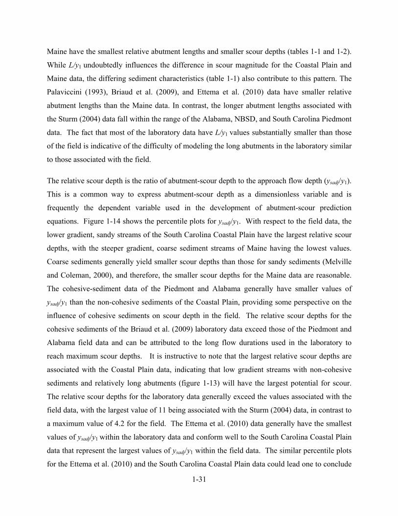
1-31
Maine have the smallest relative abutment lengths and smaller scour depths (tables 1-1 and 1-2).
While L/y1 undoubtedly influences the difference in scour magnitude for the Coastal Plain and
Maine data, the differing sediment characteristics (table 1-1) also contribute to this pattern. The
Palaviccini (1993), Briaud et al. (2009), and Ettema et al. (2010) data have smaller relative
abutment lengths than the Maine data. In contrast, the longer abutment lengths associated with
the Sturm (2004) data fall within the range of the Alabama, NBSD, and South Carolina Piedmont
data. The fact that most of the laboratory data have L/y1 values substantially smaller than those
of the field is indicative of the difficulty of modeling the long abutments in the laboratory similar
to those associated with the field.
The relative scour depth is the ratio of abutment-scour depth to the approach flow depth (ysadj/y1).
This is a common way to express abutment-scour depth as a dimensionless variable and is
frequently the dependent variable used in the development of abutment-scour prediction
equations. Figure 1-14 shows the percentile plots for ysadj/y1. With respect to the field data, the
lower gradient, sandy streams of the South Carolina Coastal Plain have the largest relative scour
depths, with the steeper gradient, coarse sediment streams of Maine having the lowest values.
Coarse sediments generally yield smaller scour depths than those for sandy sediments (Melville
and Coleman, 2000), and therefore, the smaller scour depths for the Maine data are reasonable.
The cohesive-sediment data of the Piedmont and Alabama generally have smaller values of
ysadj/y1 than the non-cohesive sediments of the Coastal Plain, providing some perspective on the
influence of cohesive sediments on scour depth in the field. The relative scour depths for the
cohesive sediments of the Briaud et al. (2009) laboratory data exceed those of the Piedmont and
Alabama field data and can be attributed to the long flow durations used in the laboratory to
reach maximum scour depths. It is instructive to note that the largest relative scour depths are
associated with the Coastal Plain data, indicating that low gradient streams with non-cohesive
sediments and relatively long abutments (figure 1-13) will have the largest potential for scour.
The relative scour depths for the laboratory data generally exceed the values associated with the
field data, with the largest value of 11 being associated with the Sturm (2004) data, in contrast to
a maximum value of 4.2 for the field. The Ettema et al. (2010) data generally have the smallest
values of ysadj/y1 within the laboratory data and conform well to the South Carolina Coastal Plain
data that represent the largest values of ysadj/y1 within the field data. The similar percentile plots
for the Ettema et al. (2010) and the South Carolina Coastal Plain data could lead one to conclude
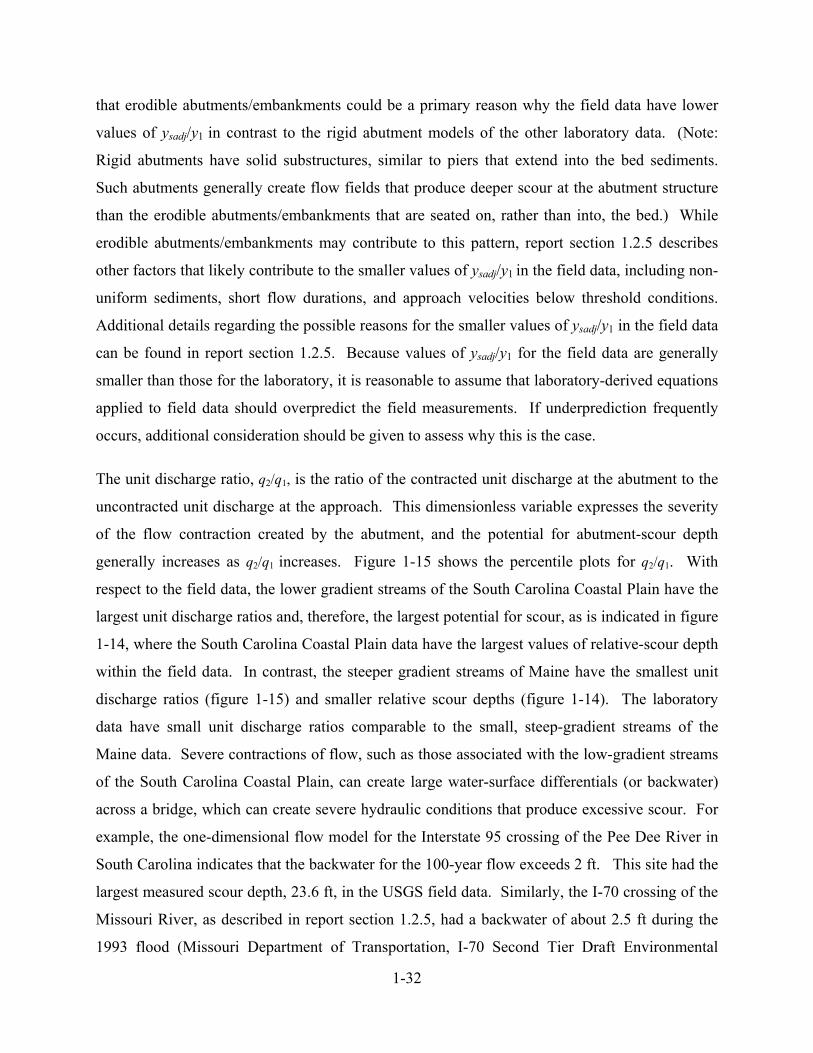
1-32
that erodible abutments/embankments could be a primary reason why the field data have lower
values of ysadj/y1 in contrast to the rigid abutment models of the other laboratory data. (Note:
Rigid abutments have solid substructures, similar to piers that extend into the bed sediments.
Such abutments generally create flow fields that produce deeper scour at the abutment structure
than the erodible abutments/embankments that are seated on, rather than into, the bed.) While
erodible abutments/embankments may contribute to this pattern, report section 1.2.5 describes
other factors that likely contribute to the smaller values of ysadj/y1 in the field data, including non-
uniform sediments, short flow durations, and approach velocities below threshold conditions.
Additional details regarding the possible reasons for the smaller values of ysadj/y1 in the field data
can be found in report section 1.2.5. Because values of ysadj/y1 for the field data are generally
smaller than those for the laboratory, it is reasonable to assume that laboratory-derived equations
applied to field data should overpredict the field measurements. If underprediction frequently
occurs, additional consideration should be given to assess why this is the case.
The unit discharge ratio, q2/q1, is the ratio of the contracted unit discharge at the abutment to the
uncontracted unit discharge at the approach. This dimensionless variable expresses the severity
of the flow contraction created by the abutment, and the potential for abutment-scour depth
generally increases as q2/q1 increases. Figure 1-15 shows the percentile plots for q2/q1. With
respect to the field data, the lower gradient streams of the South Carolina Coastal Plain have the
largest unit discharge ratios and, therefore, the largest potential for scour, as is indicated in figure
1-14, where the South Carolina Coastal Plain data have the largest values of relative-scour depth
within the field data. In contrast, the steeper gradient streams of Maine have the smallest unit
discharge ratios (figure 1-15) and smaller relative scour depths (figure 1-14). The laboratory
data have small unit discharge ratios comparable to the small, steep-gradient streams of the
Maine data. Severe contractions of flow, such as those associated with the low-gradient streams
of the South Carolina Coastal Plain, can create large water-surface differentials (or backwater)
across a bridge, which can create severe hydraulic conditions that produce excessive scour. For
example, the one-dimensional flow model for the Interstate 95 crossing of the Pee Dee River in
South Carolina indicates that the backwater for the 100-year flow exceeds 2 ft. This site had the
largest measured scour depth, 23.6 ft, in the USGS field data. Similarly, the I-70 crossing of the
Missouri River, as described in report section 1.2.5, had a backwater of about 2.5 ft during the
1993 flood (Missouri Department of Transportation, I-70 Second Tier Draft Environmental
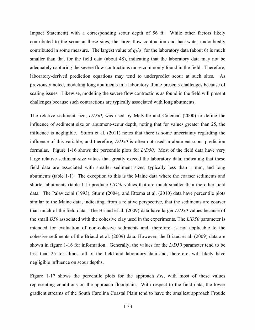
1-33
Impact Statement) with a corresponding scour depth of 56 ft. While other factors likely
contributed to the scour at these sites, the large flow contraction and backwater undoubtedly
contributed in some measure. The largest value of q2/q1 for the laboratory data (about 6) is much
smaller than that for the field data (about 48), indicating that the laboratory data may not be
adequately capturing the severe flow contractions more commonly found in the field. Therefore,
laboratory-derived prediction equations may tend to underpredict scour at such sites. As
previously noted, modeling long abutments in a laboratory flume presents challenges because of
scaling issues. Likewise, modeling the severe flow contractions as found in the field will present
challenges because such contractions are typically associated with long abutments.
The relative sediment size, L/D50, was used by Melville and Coleman (2000) to define the
influence of sediment size on abutment-scour depth, noting that for values greater than 25, the
influence is negligible. Sturm et al. (2011) notes that there is some uncertainty regarding the
influence of this variable, and therefore, L/D50 is often not used in abutment-scour prediction
formulas. Figure 1-16 shows the percentile plots for L/D50. Most of the field data have very
large relative sediment-size values that greatly exceed the laboratory data, indicating that these
field data are associated with smaller sediment sizes, typically less than 1 mm, and long
abutments (table 1-1). The exception to this is the Maine data where the coarser sediments and
shorter abutments (table 1-1) produce L/D50 values that are much smaller than the other field
data. The Palaviccini (1993), Sturm (2004), and Ettema et al. (2010) data have percentile plots
similar to the Maine data, indicating, from a relative perspective, that the sediments are coarser
than much of the field data. The Briaud et al. (2009) data have larger L/D50 values because of
the small D50 associated with the cohesive clay used in the experiments. The L/D50 parameter is
intended for evaluation of non-cohesive sediments and, therefore, is not applicable to the
cohesive sediments of the Briaud et al. (2009) data. However, the Briaud et al. (2009) data are
shown in figure 1-16 for information. Generally, the values for the L/D50 parameter tend to be
less than 25 for almost all of the field and laboratory data and, therefore, will likely have
negligible influence on scour depths.
Figure 1-17 shows the percentile plots for the approach Fr1, with most of these values
representing conditions on the approach floodplain. With respect to the field data, the lower
gradient streams of the South Carolina Coastal Plain tend to have the smallest approach Froude
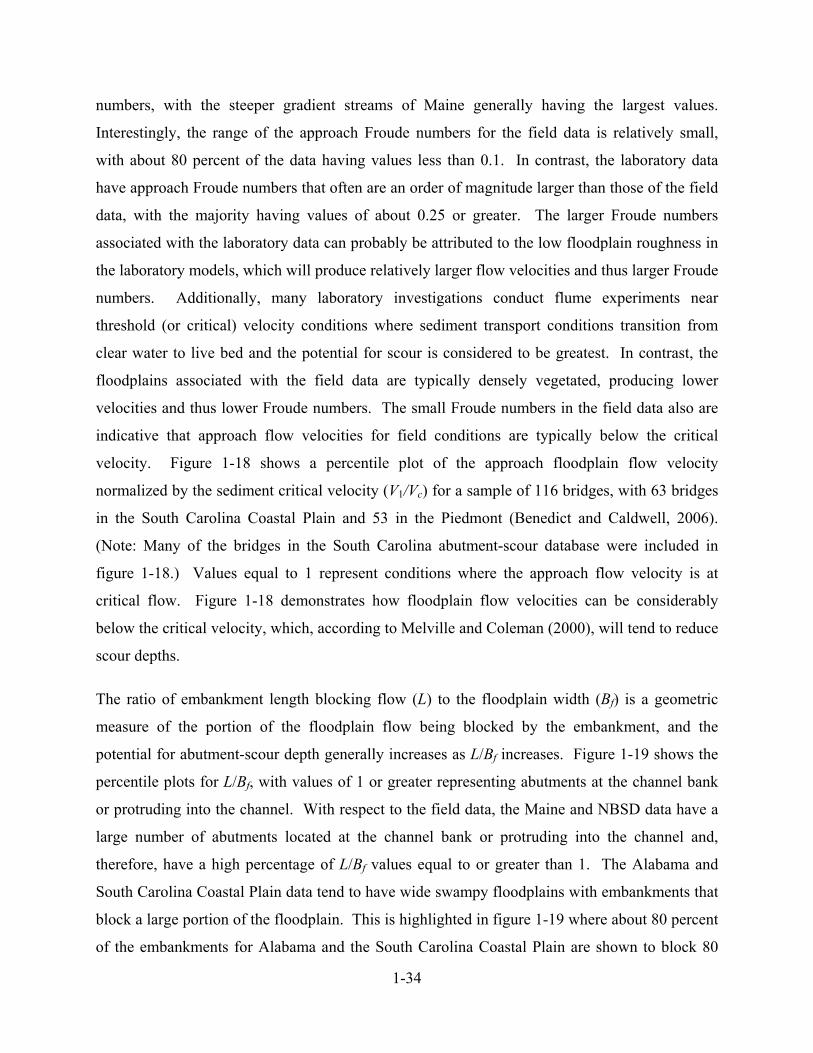
1-34
numbers, with the steeper gradient streams of Maine generally having the largest values.
Interestingly, the range of the approach Froude numbers for the field data is relatively small,
with about 80 percent of the data having values less than 0.1. In contrast, the laboratory data
have approach Froude numbers that often are an order of magnitude larger than those of the field
data, with the majority having values of about 0.25 or greater. The larger Froude numbers
associated with the laboratory data can probably be attributed to the low floodplain roughness in
the laboratory models, which will produce relatively larger flow velocities and thus larger Froude
numbers. Additionally, many laboratory investigations conduct flume experiments near
threshold (or critical) velocity conditions where sediment transport conditions transition from
clear water to live bed and the potential for scour is considered to be greatest. In contrast, the
floodplains associated with the field data are typically densely vegetated, producing lower
velocities and thus lower Froude numbers. The small Froude numbers in the field data also are
indicative that approach flow velocities for field conditions are typically below the critical
velocity. Figure 1-18 shows a percentile plot of the approach floodplain flow velocity
normalized by the sediment critical velocity (V1/Vc) for a sample of 116 bridges, with 63 bridges
in the South Carolina Coastal Plain and 53 in the Piedmont (Benedict and Caldwell, 2006).
(Note: Many of the bridges in the South Carolina abutment-scour database were included in
figure 1-18.) Values equal to 1 represent conditions where the approach flow velocity is at
critical flow. Figure 1-18 demonstrates how floodplain flow velocities can be considerably
below the critical velocity, which, according to Melville and Coleman (2000), will tend to reduce
scour depths.
The ratio of embankment length blocking flow (L) to the floodplain width (Bf) is a geometric
measure of the portion of the floodplain flow being blocked by the embankment, and the
potential for abutment-scour depth generally increases as L/Bf increases. Figure 1-19 shows the
percentile plots for L/Bf, with values of 1 or greater representing abutments at the channel bank
or protruding into the channel. With respect to the field data, the Maine and NBSD data have a
large number of abutments located at the channel bank or protruding into the channel and,
therefore, have a high percentage of L/Bf values equal to or greater than 1. The Alabama and
South Carolina Coastal Plain data tend to have wide swampy floodplains with embankments that
block a large portion of the floodplain. This is highlighted in figure 1-19 where about 80 percent
of the embankments for Alabama and the South Carolina Coastal Plain are shown to block 80
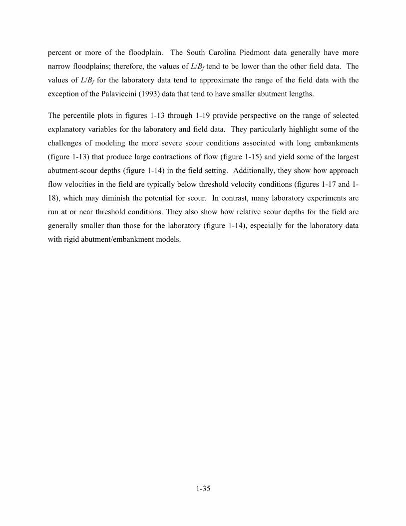
1-35
percent or more of the floodplain. The South Carolina Piedmont data generally have more
narrow floodplains; therefore, the values of L/Bf tend to be lower than the other field data. The
values of L/Bf for the laboratory data tend to approximate the range of the field data with the
exception of the Palaviccini (1993) data that tend to have smaller abutment lengths.
The percentile plots in figures 1-13 through 1-19 provide perspective on the range of selected
explanatory variables for the laboratory and field data. They particularly highlight some of the
challenges of modeling the more severe scour conditions associated with long embankments
(figure 1-13) that produce large contractions of flow (figure 1-15) and yield some of the largest
abutment-scour depths (figure 1-14) in the field setting. Additionally, they show how approach
flow velocities in the field are typically below threshold velocity conditions (figures 1-17 and 1-
18), which may diminish the potential for scour. In contrast, many laboratory experiments are
run at or near threshold conditions. They also show how relative scour depths for the field are
generally smaller than those for the laboratory (figure 1-14), especially for the laboratory data
with rigid abutment/embankment models.
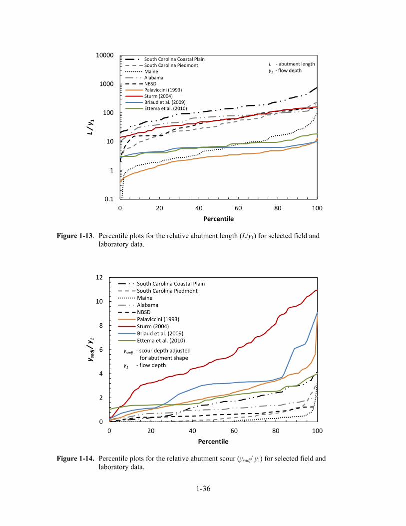
1-36
Figure 1-13. Percentile plots for the relative abutment length (L/y1) for selected field and laboratory data.
Figure 1-14. Percentile plots for the relative abutment scour (ysadj/ y1) for selected field and laboratory data.
0
2
4
6
8
10
12
0 20 40 60 80 100
y sadj / y
1
Percentile
South Carolina Coastal PlainSouth Carolina PiedmontMaineAlabamaNBSDPalaviccini (1993)Sturm (2004)Briaud et al. (2009)Ettema et al. (2010)
ysadj ‐ scour depth adjustedfor abutment shape
y1 ‐ flow depth
0.1
1
10
100
1000
10000
0 20 40 60 80 100
L / y 1
Percentile
South Carolina Coastal PlainSouth Carolina PiedmontMaineAlabamaNBSDPalaviccini (1993)Sturm (2004)Briaud et al. (2009)Ettema et al. (2010)
L ‐ abutment lengthy1 ‐ flow depth
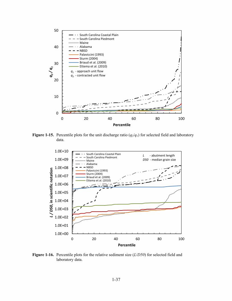
1-37
Figure 1-15. Percentile plots for the unit discharge ratio (q2/q1) for selected field and laboratory data.
Figure 1-16. Percentile plots for the relative sediment size (L/D50) for selected field and laboratory data.
0
10
20
30
40
50
0 20 40 60 80 100
q2/ q1
Percentile
South Carolina Coastal PlainSouth Carolina PiedmontMaineAlabamaNBSDPalaviccini (1993)Sturm (2004)Briaud et al. (2009)Ettema et al. (2010)
q1 ‐ approach unit flowq2 ‐ contracted unit flow
1.0E+00
1.0E+01
1.0E+02
1.0E+03
1.0E+04
1.0E+05
1.0E+06
1.0E+07
1.0E+08
1.0E+09
1.0E+10
0 20 40 60 80 100
L / D50, in scientific notation
Percentile
South Carolina Coastal PlainSouth Carolina PiedmontMaineAlabamaNBSDPalaviccini (1993)Sturm (2004)Briaud et al. (2009)Ettema et al. (2010)
L ‐ abutment lengthD50 ‐median grain size
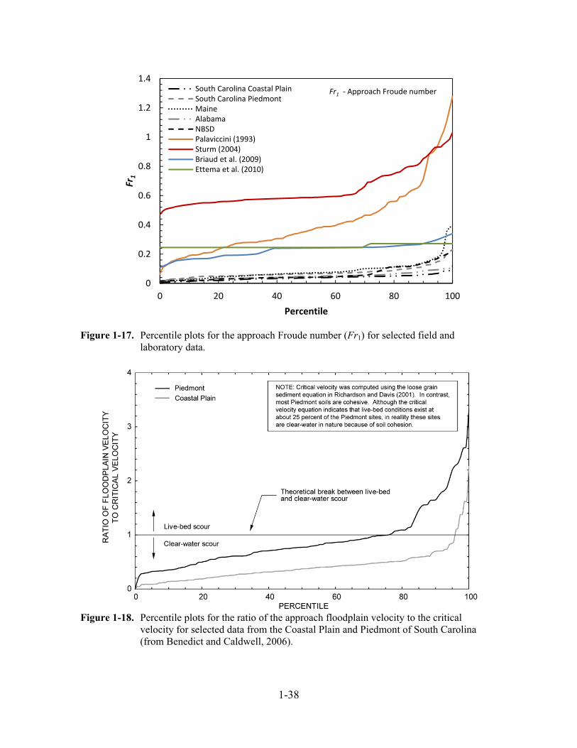
1-38
Figure 1-17. Percentile plots for the approach Froude number (Fr1) for selected field and laboratory data.
Figure 1-18. Percentile plots for the ratio of the approach floodplain velocity to the critical velocity for selected data from the Coastal Plain and Piedmont of South Carolina (from Benedict and Caldwell, 2006).
0
0.2
0.4
0.6
0.8
1
1.2
1.4
0 20 40 60 80 100
Fr1
Percentile
South Carolina Coastal PlainSouth Carolina PiedmontMaineAlabamaNBSDPalaviccini (1993)Sturm (2004)Briaud et al. (2009)Ettema et al. (2010)
Fr1 ‐ Approach Froude number
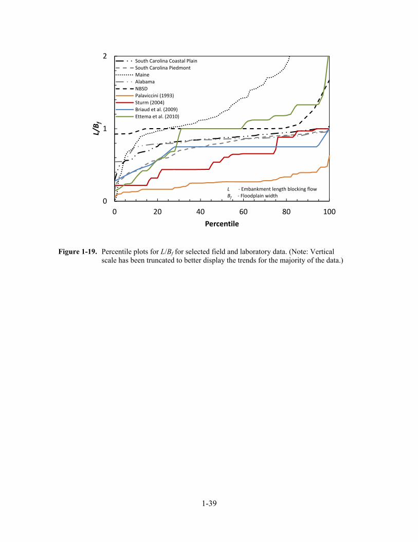
1-39
Figure 1-19. Percentile plots for L/Bf for selected field and laboratory data. (Note: Vertical
scale has been truncated to better display the trends for the majority of the data.)
0
1
2
0 20 40 60 80 100
L/Bf
Percentile
South Carolina Coastal Plain
South Carolina Piedmont
Maine
Alabama
NBSD
Palaviccini (1993)
Sturm (2004)
Briaud et al. (2009)
Ettema et al. (2010)
L ‐ Embankment length blocking flowBf ‐ Floodplain width
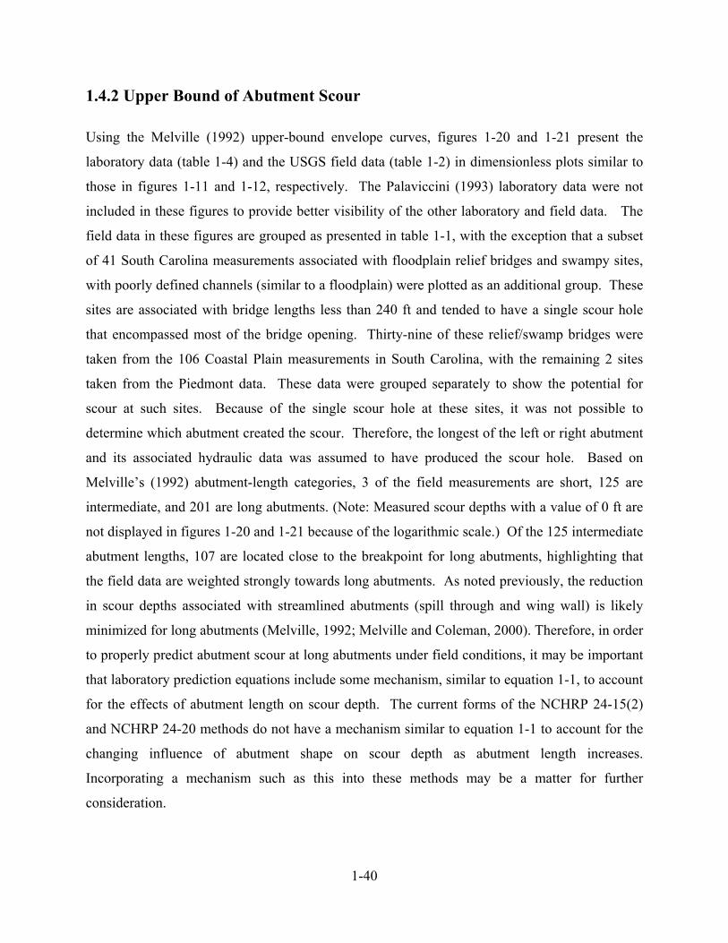
1-40
1.4.2 Upper Bound of Abutment Scour
Using the Melville (1992) upper-bound envelope curves, figures 1-20 and 1-21 present the
laboratory data (table 1-4) and the USGS field data (table 1-2) in dimensionless plots similar to
those in figures 1-11 and 1-12, respectively. The Palaviccini (1993) laboratory data were not
included in these figures to provide better visibility of the other laboratory and field data. The
field data in these figures are grouped as presented in table 1-1, with the exception that a subset
of 41 South Carolina measurements associated with floodplain relief bridges and swampy sites,
with poorly defined channels (similar to a floodplain) were plotted as an additional group. These
sites are associated with bridge lengths less than 240 ft and tended to have a single scour hole
that encompassed most of the bridge opening. Thirty-nine of these relief/swamp bridges were
taken from the 106 Coastal Plain measurements in South Carolina, with the remaining 2 sites
taken from the Piedmont data. These data were grouped separately to show the potential for
scour at such sites. Because of the single scour hole at these sites, it was not possible to
determine which abutment created the scour. Therefore, the longest of the left or right abutment
and its associated hydraulic data was assumed to have produced the scour hole. Based on
Melville’s (1992) abutment-length categories, 3 of the field measurements are short, 125 are
intermediate, and 201 are long abutments. (Note: Measured scour depths with a value of 0 ft are
not displayed in figures 1-20 and 1-21 because of the logarithmic scale.) Of the 125 intermediate
abutment lengths, 107 are located close to the breakpoint for long abutments, highlighting that
the field data are weighted strongly towards long abutments. As noted previously, the reduction
in scour depths associated with streamlined abutments (spill through and wing wall) is likely
minimized for long abutments (Melville, 1992; Melville and Coleman, 2000). Therefore, in order
to properly predict abutment scour at long abutments under field conditions, it may be important
that laboratory prediction equations include some mechanism, similar to equation 1-1, to account
for the effects of abutment length on scour depth. The current forms of the NCHRP 24-15(2)
and NCHRP 24-20 methods do not have a mechanism similar to equation 1-1 to account for the
changing influence of abutment shape on scour depth as abutment length increases.
Incorporating a mechanism such as this into these methods may be a matter for further
consideration.

1-41
Figures 1-20 and 1-21 clearly show that the upper bound of the field data is below that of the
laboratory data. For the case of long abutments, figure 1-21 indicates that the upper bound for the
laboratory data is approximately 11 times the flow depth. In contrast, the upper bound for the
field data is 4.2 times the flow depth. As noted previously (report section 1.2.5), field conditions
such as non-uniform sediments, approach velocities below threshold conditions, and short flow
durations will tend to limit the ability to develop equilibrium-scour depths in the field that are
comparable to those of the laboratory. This is part of the reason why the upper bound of the field
data is less than the upper bound of the laboratory data.
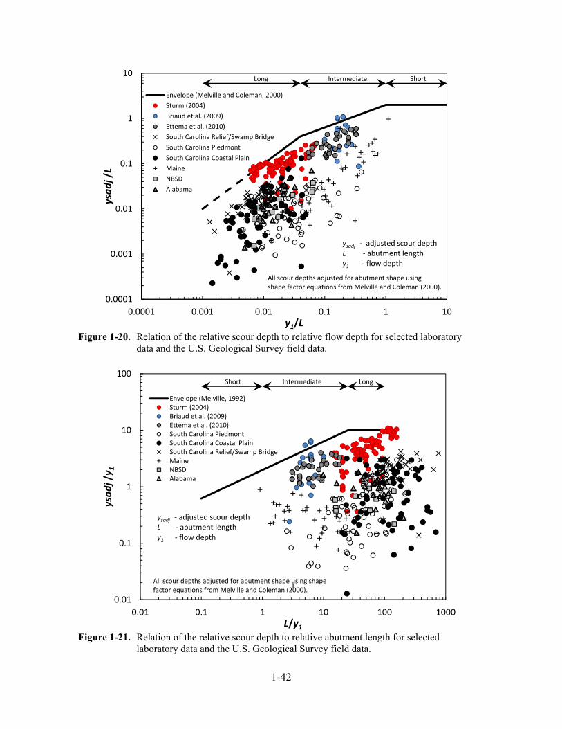
1-42
Figure 1-20. Relation of the relative scour depth to relative flow depth for selected laboratory data and the U.S. Geological Survey field data.
Figure 1-21. Relation of the relative scour depth to relative abutment length for selected laboratory data and the U.S. Geological Survey field data.
0.0001
0.001
0.01
0.1
1
10
0.0001 0.001 0.01 0.1 1 10
ysadj/L
y1/L
Envelope (Melville and Coleman, 2000)
Sturm (2004)
Briaud et al. (2009)
Ettema et al. (2010)
South Carolina Relief/Swamp Bridge
South Carolina Piedmont
South Carolina Coastal Plain
Maine
NBSD
Alabama
All scour depths adjusted for abutment shape usingshape factor equations from Melville and Coleman (2000).
ysadj ‐ adjusted scour depthL ‐ abutment lengthy1 ‐ flow depth
Long Intermediate Short
0.01
0.1
1
10
100
0.01 0.1 1 10 100 1000
ysadj/y 1
L/y1
Envelope (Melville, 1992)Sturm (2004)Briaud et al. (2009)Ettema et al. (2010)South Carolina PiedmontSouth Carolina Coastal PlainSouth Carolina Relief/Swamp BridgeMaineNBSDAlabama
All scour depths adjusted for abutment shape using shapefactor equations from Melville and Coleman (2000).
ysadj ‐ adjusted scour depthL ‐ abutment lengthy1 ‐ flow depth
LongIntermediateShort
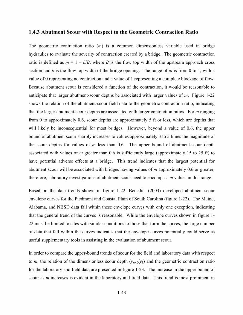
1-43
1.4.3 Abutment Scour with Respect to the Geometric Contraction Ratio
The geometric contraction ratio (m) is a common dimensionless variable used in bridge
hydraulics to evaluate the severity of contraction created by a bridge. The geometric contraction
ratio is defined as m = 1 – b/B, where B is the flow top width of the upstream approach cross
section and b is the flow top width of the bridge opening. The range of m is from 0 to 1, with a
value of 0 representing no contraction and a value of 1 representing a complete blockage of flow.
Because abutment scour is considered a function of the contraction, it would be reasonable to
anticipate that larger abutment-scour depths be associated with larger values of m. Figure 1-22
shows the relation of the abutment-scour field data to the geometric contraction ratio, indicating
that the larger abutment-scour depths are associated with larger contraction ratios. For m ranging
from 0 to approximately 0.6, scour depths are approximately 5 ft or less, which are depths that
will likely be inconsequential for most bridges. However, beyond a value of 0.6, the upper
bound of abutment scour sharply increases to values approximately 3 to 5 times the magnitude of
the scour depths for values of m less than 0.6. The upper bound of abutment-scour depth
associated with values of m greater than 0.6 is sufficiently large (approximately 15 to 25 ft) to
have potential adverse effects at a bridge. This trend indicates that the largest potential for
abutment scour will be associated with bridges having values of m approximately 0.6 or greater;
therefore, laboratory investigations of abutment scour need to encompass m values in this range.
Based on the data trends shown in figure 1-22, Benedict (2003) developed abutment-scour
envelope curves for the Piedmont and Coastal Plain of South Carolina (figure 1-22). The Maine,
Alabama, and NBSD data fall within these envelope curves with only one exception, indicating
that the general trend of the curves is reasonable. While the envelope curves shown in figure 1-
22 must be limited to sites with similar conditions to those that form the curves, the large number
of data that fall within the curves indicates that the envelope curves potentially could serve as
useful supplementary tools in assisting in the evaluation of abutment scour.
In order to compare the upper-bound trends of scour for the field and laboratory data with respect
to m, the relation of the dimensionless scour depth (ysadj/y1) and the geometric contraction ratio
for the laboratory and field data are presented in figure 1-23. The increase in the upper bound of
scour as m increases is evident in the laboratory and field data. This trend is most prominent in
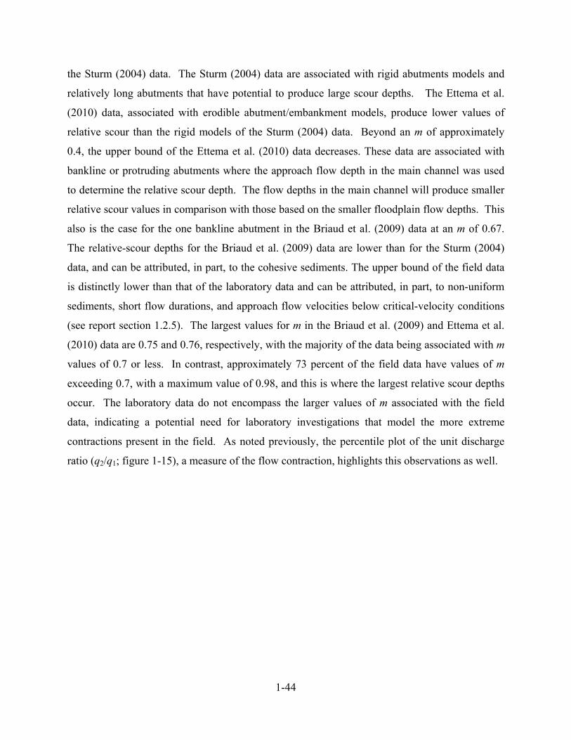
1-44
the Sturm (2004) data. The Sturm (2004) data are associated with rigid abutments models and
relatively long abutments that have potential to produce large scour depths. The Ettema et al.
(2010) data, associated with erodible abutment/embankment models, produce lower values of
relative scour than the rigid models of the Sturm (2004) data. Beyond an m of approximately
0.4, the upper bound of the Ettema et al. (2010) data decreases. These data are associated with
bankline or protruding abutments where the approach flow depth in the main channel was used
to determine the relative scour depth. The flow depths in the main channel will produce smaller
relative scour values in comparison with those based on the smaller floodplain flow depths. This
also is the case for the one bankline abutment in the Briaud et al. (2009) data at an m of 0.67.
The relative-scour depths for the Briaud et al. (2009) data are lower than for the Sturm (2004)
data, and can be attributed, in part, to the cohesive sediments. The upper bound of the field data
is distinctly lower than that of the laboratory data and can be attributed, in part, to non-uniform
sediments, short flow durations, and approach flow velocities below critical-velocity conditions
(see report section 1.2.5). The largest values for m in the Briaud et al. (2009) and Ettema et al.
(2010) data are 0.75 and 0.76, respectively, with the majority of the data being associated with m
values of 0.7 or less. In contrast, approximately 73 percent of the field data have values of m
exceeding 0.7, with a maximum value of 0.98, and this is where the largest relative scour depths
occur. The laboratory data do not encompass the larger values of m associated with the field
data, indicating a potential need for laboratory investigations that model the more extreme
contractions present in the field. As noted previously, the percentile plot of the unit discharge
ratio (q2/q1; figure 1-15), a measure of the flow contraction, highlights this observations as well.
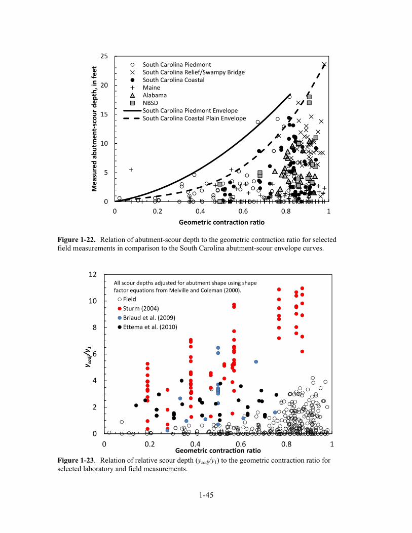
1-45
Figure 1-22. Relation of abutment-scour depth to the geometric contraction ratio for selected field measurements in comparison to the South Carolina abutment-scour envelope curves.
Figure 1-23. Relation of relative scour depth (ysadj/y1) to the geometric contraction ratio for selected laboratory and field measurements.
0
5
10
15
20
25
0 0.2 0.4 0.6 0.8 1
Measured abutm
ent‐scour depth, in feet
Geometric contraction ratio
South Carolina PiedmontSouth Carolina Relief/Swampy BridgeSouth Carolina CoastalMaineAlabamaNBSDSouth Carolina Piedmont EnvelopeSouth Carolina Coastal Plain Envelope
0
2
4
6
8
10
12
0 0.2 0.4 0.6 0.8 1
y sadj/y 1
Geometric contraction ratio
Field
Sturm (2004)
Briaud et al. (2009)
Ettema et al. (2010)
All scour depths adjusted for abutment shape using shapefactor equations from Melville and Coleman (2000).
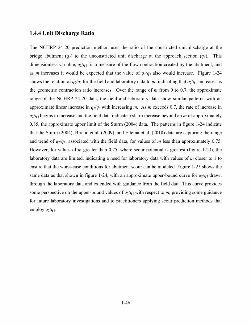
1-46
1.4.4 Unit Discharge Ratio
The NCHRP 24-20 prediction method uses the ratio of the constricted unit discharge at the
bridge abutment (q2) to the unconstricted unit discharge at the approach section (q1). This
dimensionless variable, q2/q1, is a measure of the flow contraction created by the abutment, and
as m increases it would be expected that the value of q2/q1 also would increase. Figure 1-24
shows the relation of q2/q1 for the field and laboratory data to m, indicating that q2/q1 increases as
the geometric contraction ratio increases. Over the range of m from 0 to 0.7, the approximate
range of the NCHRP 24-20 data, the field and laboratory data show similar patterns with an
approximate linear increase in q2/q1 with increasing m. As m exceeds 0.7, the rate of increase in
q2/q1 begins to increase and the field data indicate a sharp increase beyond an m of approximately
0.85, the approximate upper limit of the Sturm (2004) data. The patterns in figure 1-24 indicate
that the Sturm (2004), Briaud et al. (2009), and Ettema et al. (2010) data are capturing the range
and trend of q2/q1, associated with the field data, for values of m less than approximately 0.75.
However, for values of m greater than 0.75, where scour potential is greatest (figure 1-23), the
laboratory data are limited, indicating a need for laboratory data with values of m closer to 1 to
ensure that the worst-case conditions for abutment scour can be modeled. Figure 1-25 shows the
same data as that shown in figure 1-24, with an approximate upper-bound curve for q2/q1 drawn
through the laboratory data and extended with guidance from the field data. This curve provides
some perspective on the upper-bound values of q2/q1 with respect to m, providing some guidance
for future laboratory investigations and to practitioners applying scour prediction methods that
employ q2/q1.
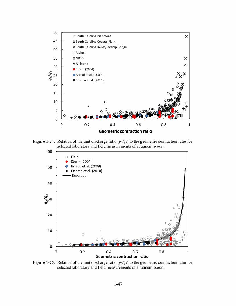
1-47
Figure 1-24. Relation of the unit discharge ratio (q2/q1) to the geometric contraction ratio for selected laboratory and field measurements of abutment scour.
Figure 1-25. Relation of the unit discharge ratio (q2/q1) to the geometric contraction ratio for selected laboratory and field measurements of abutment scour.
0
5
10
15
20
25
30
35
40
45
50
0 0.2 0.4 0.6 0.8 1
q2/q
1
Geometric contraction ratio
South Carolina Piedmont
South Carolina Coastal Plain
South Carolina Relief/Swamp Bridge
Maine
NBSD
Alabama
Sturm (2004)
Briaud at al. (2009)
Ettema et al. (2010)
0
10
20
30
40
50
60
0 0.2 0.4 0.6 0.8 1
q2/q
1
Geometric contraction ratio
FieldSturm (2004)Briaud et al. (2009)Ettema et al. (2010) Envelope
2-1
CHAPTER 2
APPLICATION PROCEDURE FOR THE NCHRP 24-20
PREDICTION METHOD
2.1 Introduction
The NCHRP 24-20 report provides general guidance for applying the abutment-scour prediction
method at a selected bridge site. Hydraulic Engineering Circular No. 18 (Arneson et al. 2012; for
remainder of this section will be noted as HEC-18 without the reference) provides additional
application guidance. These two sources were used to develop the procedure for applying the
NCHRP 24-20 method to the laboratory and USGS field data. Additionally, Dr. Robert Ettema,
the Principal Investigator for NCHRP 24-20, and Mr. Bart Bergendahl of the Federal Highway
Administration were consulted in the development of the this procedure and were provided
opportunity for review and comment. A brief description of the application steps follows.
2.2 Summary of NCHRP 24-20 Scour Prediction Method
The NCHRP Project 24-20 was an extensive laboratory investigation of abutment scour that
produced new insight into the mechanics of abutment scour and led to a method for estimating
abutment-scour depth in compound channels. The method encompasses a range of abutment-
scour conditions including (A) abutments set near or in the main channel, (B) abutments on the
floodplain set well back from the main channel, (C) abutments with breached embankments and
exposed abutment column, and (D) abutment-scour associated with geotechnical failure at a
location at some distance from the end of the abutment. Scour conditions C and D were not
evaluated in this investigation. A unique feature about the NCHRP 24-20 laboratory
investigation was the use of abutment models having various combinations of erodible and non-
erodible floodplains, embankments, and abutment substructures. Such characteristics are
thought to better represent the range of conditions frequently found in the field, where
embankment and abutment substructures can be susceptible to scour and possible failure.
Previous investigations of abutment scour typically used non-erodible, rigid abutment models
2-2
having an abutment substructure consisting of a vertical wall at the abutment toe extending into
the bed, similar to a sheet-pile skirt. These rigid abutment models with the vertical wall
substructures tend to strengthen flow turbulence near the abutment, increasing the potential for
scour. In contrast, the NCHRP 24-20 abutment models used a variety of erodible and non-
erodible embankment and abutment substructures that primarily excluded the vertical wall
substructure associated with many previous laboratory investigations. These models better
represent embankments and abutment substructures for many field sites and will tend to reduce
the potential for scour in contrast to the rigid abutment models. Additionally, the erodible
embankments/abutments will provide some measure of hydraulic relief in the cases where the
embankment/abutment breaches under high-flow conditions, further reducing the potential for
scour. For Scour Condition A, where the abutment is set near the main channel, the NCHRP 24-
20 laboratory tests consisted of non-erodible (fixed) floodplains and abutments, as well as
erodible floodplains and abutments, with the embankment and abutment armored with riprap.
For the fixed conditions, scour was forced to occur in the main channel under live-bed scour
conditions and produced larger scour depths than the erodible conditions produced. Because of
the complexity of flow and scour patterns for Scour Condition A, NCHRP 24-20 developed
scour prediction methods based on data from the fixed floodplain and abutment model, providing
a more conservative estimate of abutment scour. For Scour Condition B, where the abutment is
well set back from the main channel, the laboratory model used in developing the design
procedure primarily consisted of an erodible floodplain and abutment, with the embankment and
abutment armored with rip rap. Under these conditions, the abutment and embankment could
erode, providing some hydraulic relief that tended to reduce abutment scour. Additionally, the
abutment substructure for these models typically did not consist of a rigid wall below the bed,
further reducing the potential for scour.
The laboratory models used to develop the NCHRP 24-20 method are distinctly different from
the models used to develop other abutment-scour prediction equations, such as the Froehlich
(1989) equation and the NCHRP 24-15(2) method (Briaud et al. 2009) that used rigid
abutments/embankments. As such, it is likely that the NCHRP 24-20 method will produce
smaller values of predicted scour than prediction equations developed from rigid abutment
models. This will most likely be evident for the case of Scour Condition B, where erodible
embankments were used, but less so for Scour Condition A where fixed embankments/abutments
2-3
were used. Additionally, when the NCHRP 24-20 method is applied to laboratory or field data
that is more representative of a rigid abutment model, it is likely that the NCHRP 24-20 will
produce some underprediction of scour for such conditions. Again, this will likely be more
evident for Scour Condition B than for A. With the exception of the NCHRP 24-20 data, the
majority of laboratory data used in the current (2015) investigation [NCHRP Project 24-20(2)]
represents scour at non-erodible rigid abutments, and therefore, application of the NCHRP 24-20
method to these data will likely produce some underprediction. Additionally, the field data are
thought to largely represent abutment scour where the road embankment and abutment
substructures did not appreciably erode. While not identical, this field condition is similar to a
rigid laboratory model, and therefore, application of the NCHRP 24-20 method to these field
data may produce some underprediction. These differing scour conditions associated with the
NCHRP 24-20 prediction method and the laboratory and field data should be kept in mind when
reviewing results of this investigation.
When using the NCHRP 24-20 method it is important to apply the procedure to the correct scour
condition. For abutments with Scour Conditions A and B, the NCHRP 24-20 abutment-scour
method assumes that abutment scour is a function of contraction scour at a long contraction as
represented by the following equation:
YMAX = YC (2-1)
where
YMAX is the maximum flow depth in the abutment scour area, in feet (figure 2-1);
YC is the mean flow depth of the contraction scour associated with a long contraction,
in feet (figure 2-1); and
is an amplification factor that accounts for additional scour (beyond the
contraction scour) at the abutment associated with the non-uniform flow
distribution and macro-turbulence structures in the vicinity of the abutment.
The conceptual model represented in equation 2-1 has been used by other researchers (Laursen,
1963; Chang and Davis, 1998 and 1999; Sturm, 2004); however, Ettema et al. (2010) developed
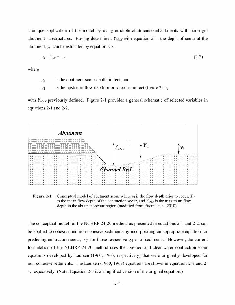
2-4
a unique application of the model by using erodible abutments/embankments with non-rigid
abutment substructures. Having determined YMAX with equation 2-1, the depth of scour at the
abutment, ys, can be estimated by equation 2-2.
ys = YMAX – y1 (2-2)
where
ys is the abutment-scour depth, in feet, and
y1 is the upstream flow depth prior to scour, in feet (figure 2-1),
with YMAX previously defined. Figure 2-1 provides a general schematic of selected variables in
equations 2-1 and 2-2.
Figure 2-1. Conceptual model of abutment scour where y1 is the flow depth prior to scour, YC is the mean flow depth of the contraction scour, and YMAX is the maximum flow depth in the abutment-scour region (modified from Ettema et al. 2010).
The conceptual model for the NCHRP 24-20 method, as presented in equations 2-1 and 2-2, can
be applied to cohesive and non-cohesive sediments by incorporating an appropriate equation for
predicting contraction scour, YC, for those respective types of sediments. However, the current
formulation of the NCHRP 24-20 method uses the live-bed and clear-water contraction-scour
equations developed by Laursen (1960; 1963, respectively) that were originally developed for
non-cohesive sediments. The Laursen (1960; 1963) equations are shown in equations 2-3 and 2-
4, respectively. (Note: Equation 2-3 is a simplified version of the original equation.)
Abutment
y YYMAXC
1
Channel Bed

2-5
⁄ (2-3)
⁄
⁄ (2-4)
where
q1 is the unconstricted unit discharge at the approach section, in square feet per
second ; (Note: The unit discharge, also called unit flow, represents the unit width
flow at the approach floodplain (qf1) or the main channel (qmc1) as shown in figure
2-2, and can be estimated in several ways: (1) by dividing the flow through the
selected section by the corresponding flow top width, or (2) multiplying the flow
depth and velocity at a given location in the cross section.);
q2 is the contracted unit discharge at the bridge abutment (figure 2-2) accounting for
non-uniform flow distribution at the abutment, in square feet per second;
Ku is a units conversion factor equal to 11.17 for English units;
D50 is the median particle size of the bed sediment, in feet; and
other variables are as previously defined.
Equation 2-4 is intended for non-cohesive sediments; therefore, HEC-18 recommends limiting
the D50 to a value of 0.000656 ft [0.2 millimeter (mm)].
For setback abutments located on the floodplain, the unit discharges q1 and q2 will generally
reflect flows on the upstream approach floodplain (qf1) and the associated overbank at the bridge
(qf2), respectively, as shown in figure 2-2. For abutments located at the channel banks or
protruding into the channel, the unit discharges q1 and q2 will generally reflect flows in the
upstream approach main channel (qmc1) and the main channel at the bridge (qmc2), respectively
(figure 2-2). Guidance for estimating q1 and q2 is provided in NCHRP 24-20 and HEC-18 and is
reviewed later. Upon obtaining an estimate of YC, the maximum flow depth in the abutment
scour area, YMAX, can be estimated by applying the amplification factor, , as shown in equation
2-1.
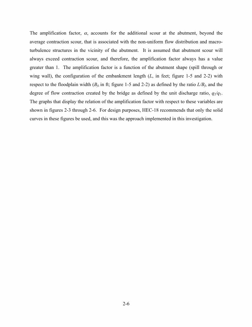
2-6
The amplification factor, , accounts for the additional scour at the abutment, beyond the
average contraction scour, that is associated with the non-uniform flow distribution and macro-
turbulence structures in the vicinity of the abutment. It is assumed that abutment scour will
always exceed contraction scour, and therefore, the amplification factor always has a value
greater than 1. The amplification factor is a function of the abutment shape (spill through or
wing wall), the configuration of the embankment length (L, in feet; figure 1-5 and 2-2) with
respect to the floodplain width (Bf, in ft; figure 1-5 and 2-2) as defined by the ratio L/Bf, and the
degree of flow contraction created by the bridge as defined by the unit discharge ratio, q2/q1.
The graphs that display the relation of the amplification factor with respect to these variables are
shown in figures 2-3 through 2-6. For design purposes, HEC-18 recommends that only the solid
curves in these figures be used, and this was the approach implemented in this investigation.
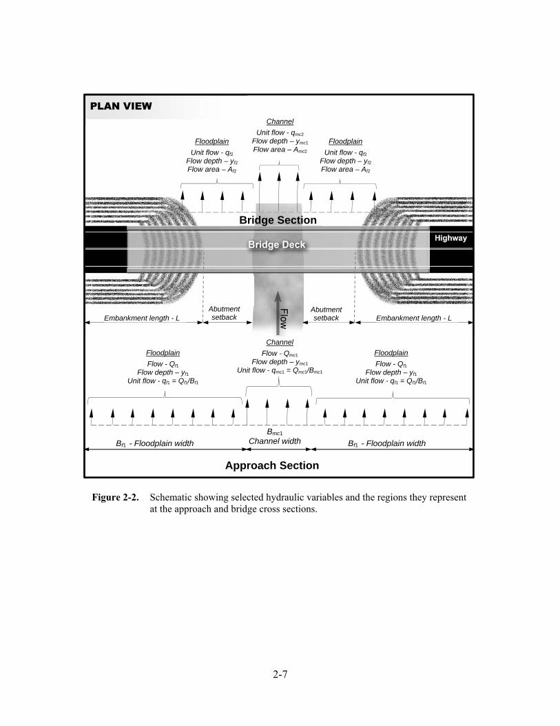
2-7
Figure 2-2. Schematic showing selected hydraulic variables and the regions they represent at the approach and bridge cross sections.
Floodplain
Flow - Qf1 Flow depth – yf1
Unit flow - qf1 = Qf1/Bf1
Approach Section
Bf1 - Floodplain width Bf1 - Floodplain width
Bmc1 Channel width
Floodplain
Flow - Qf1 Flow depth – yf1
Unit flow - qf1 = Qf1/Bf1
Channel
Flow - Qmc1 Flow depth – ymc1
Unit flow - qmc1 = Qmc1/Bmc1
Floodplain
Unit flow - qf2
Flow depth – yf2
Flow area – Af2
Channel
Unit flow - qmc2
Flow depth – ymc1
Flow area – Amc2 Floodplain
Unit flow - qf2
Flow depth – yf2
Flow area – Af2
Bridge Section
Embankment length - L Embankment length - L Abutment setback
Abutment setback
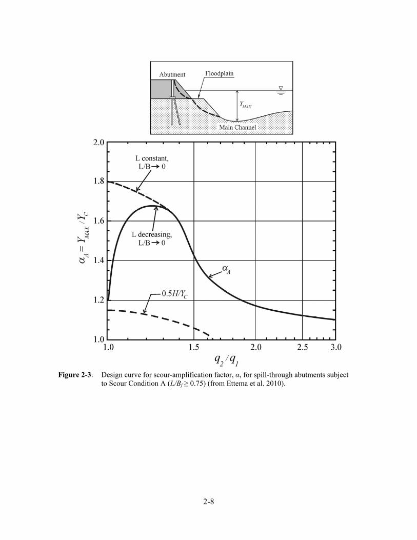
2-8
Figure 2-3. Design curve for scour-amplification factor, α, for spill-through abutments subject to Scour Condition A (L/Bf ≥ 0.75) (from Ettema et al. 2010).
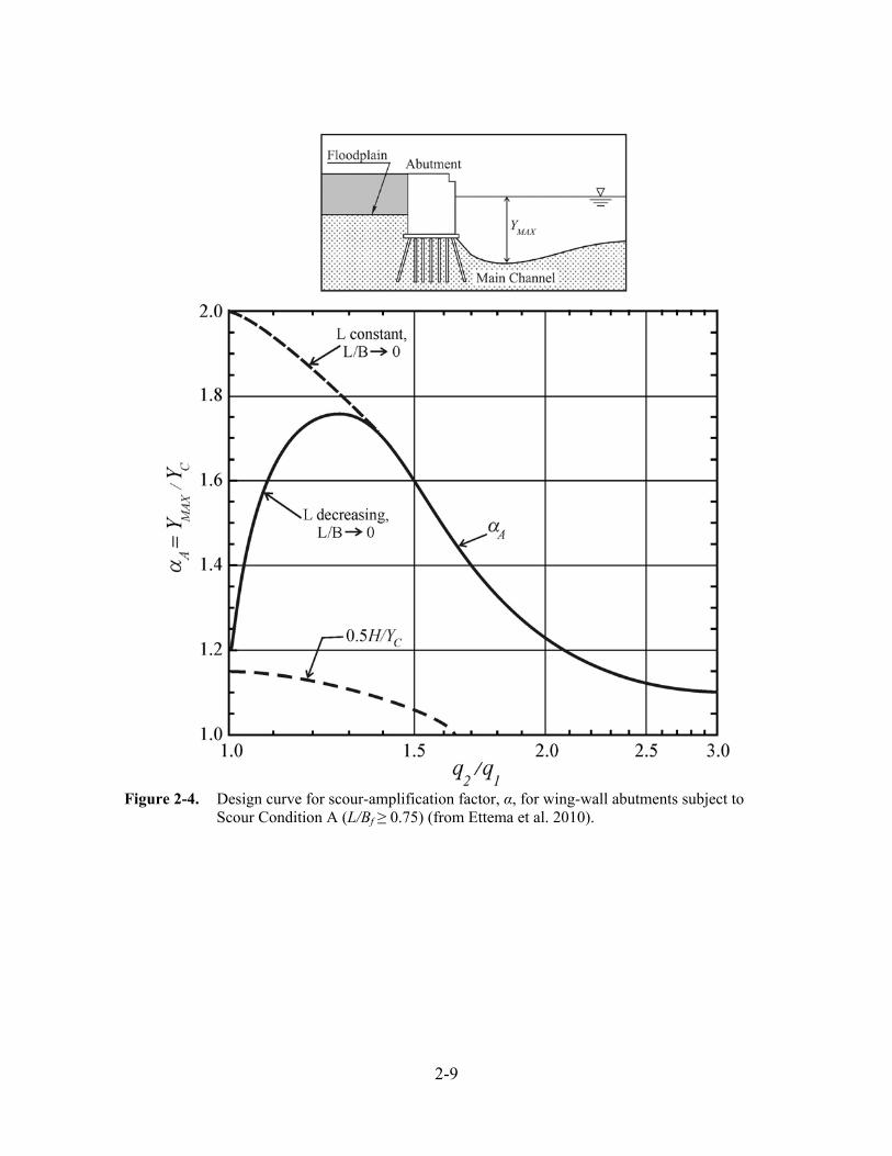
2-9
Figure 2-4. Design curve for scour-amplification factor, α, for wing-wall abutments subject to Scour Condition A (L/Bf ≥ 0.75) (from Ettema et al. 2010).
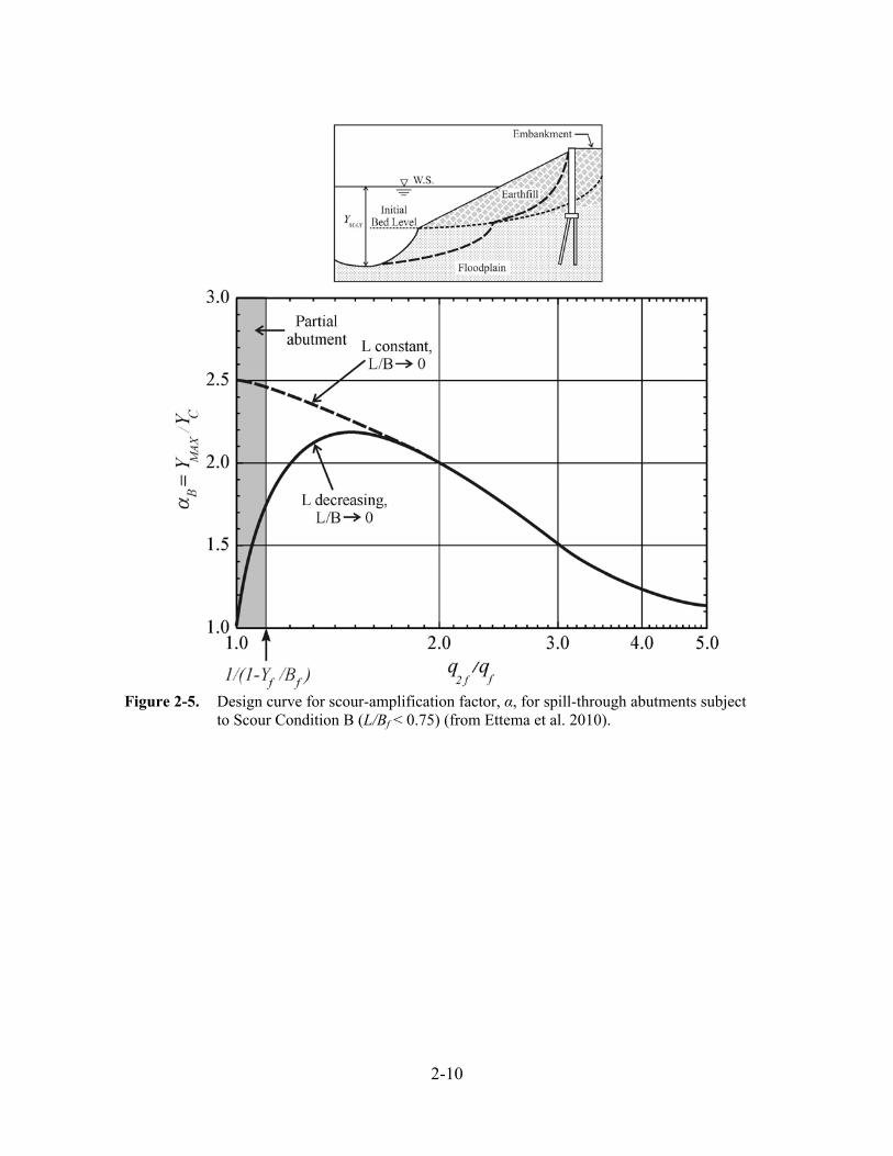
2-10
Figure 2-5. Design curve for scour-amplification factor, α, for spill-through abutments subject to Scour Condition B (L/Bf < 0.75) (from Ettema et al. 2010).
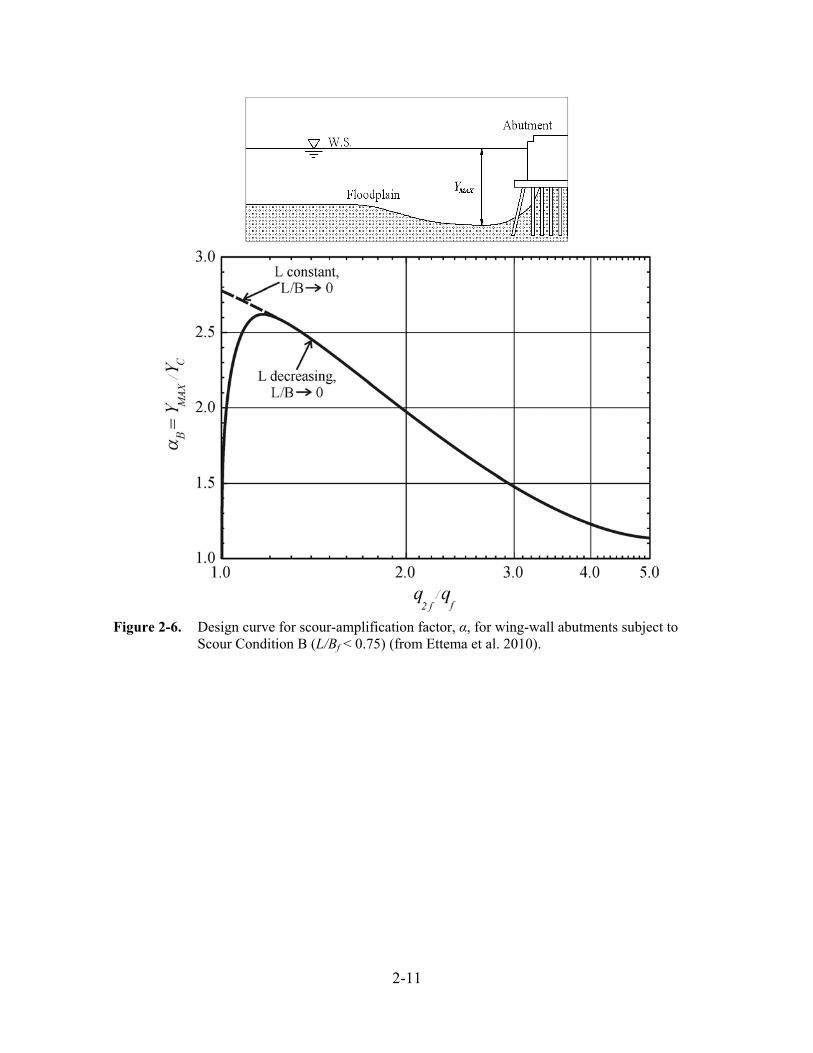
2-11
Figure 2-6. Design curve for scour-amplification factor, α, for wing-wall abutments subject to Scour Condition B (L/Bf < 0.75) (from Ettema et al. 2010).
2-12
2.3 General Procedure for Application of NCHRP 24-20 to the
Laboratory and the USGS Field Data
Field conditions associated with the riverine environment are typically more complex than those
of the laboratory. Channel geometry, surface roughness, sediment characteristics, and flow
distributions can be highly variable in the field in contrast to the controlled and idealized
environment of the laboratory. The disparity between laboratory and field conditions can present
challenges for selecting appropriate field values for application to laboratory-derived scour
prediction methods. To assist the practitioner, NCHRP 24-20 and HEC-18 present procedures
for applying the NCHRP 24-20 method to field sites. The procedures described in HEC-18 were
given preference in this investigation, and additional details can be found in HEC-18. A brief
review of the steps used in applying the NCHRP 24-20 method to the USGS field data follows.
These same general procedures were used in the application of the NCHRP 24-20 method to the
laboratory data.
1. Compile laboratory and USGS field data
The previously described laboratory and USGS field data (tables 1-1 and 1-3) were
reviewed, and data pertinent for application to the NCHRP 24-20 method were entered
into a spreadsheet. These data included selected hydraulic, sediment, and bridge-
geometry characteristics as described in table 2-1.
2. Determine the Scour Condition (A or B) for the abutment of interest
The following criteria were used to determine the Scour Condition (A or B) for the
abutment of interest:
Scour condition A was assumed when
-L/Bf ≥ 0.75;
Scour condition B was assumed when
-L/Bf < 0.75.
Variables are as previously defined.

2-13
Table 2-1. Description of selected field data used in the application of the NCHRP 24-20 abutment-scour prediction method.
Hydraulic characteristics at upstream approach cross section
Left floodplain - Flow - Flow area - Average flow depth - Top width
Channel
Right floodplain
Hydraulics characteristics at bridge cross section
Left floodplain - Flow - Flow area - Average flow depth - Channel top width or width of the floodplain
Channel
Right floodplain
Abutment
Left
- Measured scour depth - Abutment type (spill through or wing wall) - Embankment length blocking flow - Blocked flow - Blocked area - Blocked flow depth (average) - Blocked flow velocity (average) - Embankment skew - Abutment toe to top-of-bank set back distance - Median grain size of sediment - General classification of sediment at the abutments
as cohesive or non-cohesive
Right
2-14
3. Determine the unconstricted unit discharge in the upstream approach cross section
When available, a two-dimensional flow model can be used to estimate the unconstricted
unit discharge, q1, at the approach cross section. However, for unconstricted cross
sections, such as an upstream approach cross section, a one-dimensional flow model can
provide reasonable estimates of this unit discharge. When a one-dimensional flow model
is used at a bridge site, NCHRP 24-20 and HEC-18 recommend the following procedure
for estimating the unconstricted unit discharge. In the current investigation, the bridge
sites associated with the field data had only one-dimensional flow models; therefore, this
was the method used. This approach also was used with the laboratory data.
Approach floodplain (left or right; see figure 2-2):
qf1 = Qf1/Bf1 (2-5)
where
qf1 is the unit discharge on the left or right approach floodplain, in square feet
per second;
Qf1 is the flow in the left or right approach floodplain, in cubic feet per
second; and
Bf1 is the top width of the left or right approach floodplain, in feet.
Approach main channel (see figure 2-2):
qmc1 = Qmc1/Bmc1 (2-6)
where
qmc1 is the unit discharge in the approach main channel, in square feet per
second;
Qmc1 is the flow in the approach main channel, in cubic feet per second; and
Bmc1 is the top width of the approach main channel, in feet.
4. Determine the unit discharge in the bridge cross section
Flow distributions at a contracted cross section, such as a bridge, are more complex than
flow distributions associated with an unconstricted cross section. NCHRP 24-20 and
2-15
HEC-18 recommend, when possible, the use of a two-dimensional flow model to estimate
contracted unit discharge at an abutment. A one-dimensional flow model does not capture
well the increased velocities near the abutment of a contracted bridge opening; therefore,
special consideration must be given to estimating the unit discharge at a bridge when a
one-dimensional flow model is used. To assure conservative estimates of unit discharge
at a bridge abutment when using a one-dimensional flow model, HEC-18 recommends
use of the setback ratio (SBR) method as presented in HEC-23 (Lagasse et al. 2009) for
estimating flow velocities at bridge abutments that, in turn, can be used to estimate the
unit discharge. The SBR is the ratio of the abutment setback length (distance from the
abutment toe to the top of bank at the main channel; figures 1-5 and 2-2), for the
respective abutment, to the average flow depth in the main channel (ymc2) at the bridge.
Lagasse et al. (2006) investigated the SBR method by using two-dimensional flow
models of hypothetical abutments and concluded that the SBR method is well suited for
determining velocity at an abutment if the estimated velocity does not exceed the
maximum velocity in the main channel. The SBR method assumes that for relatively
short bridges with small abutment setbacks (SBR ≤ 5) the average velocity through the
full bridge (overbanks and channel) will provide a reasonable estimate of the increased
velocities at an abutment as well as velocities in the main channel. For relatively long
bridges with abutments set back some distance from the main-channel banks (SBR > 5),
the SBR method assumes that all of the flow on the left or right upstream approach
floodplain will pass through the corresponding overbank flow area at the bridge,
providing estimates of the increased velocity at the abutment. Because the bridge sites
associated with the USGS field data only have one-dimensional flow models, the SBR
method was used in the current investigation. A brief description of the steps used to
apply the SBR method to the USGS field sites follows. Additional details are presented
in HEC-18.
The SBR was calculated for the left and right abutments at a site of interest by dividing
the setback length (distance from the abutment toe to the top of bank at the main channel;
figures 1-5 and 2-2), for the respective abutment, by the average flow depth in the main
channel at the bridge. Based on the SBR values, the following procedures were used to
2-16
estimate the flow velocity and unit discharge in the overbanks and main channel at the
bridge.
SBR ≤ 5 at the left and right abutments
A general schematic for the SBR ≤ 5 is shown in figure 2-7. The left and right
abutment configurations can have several combinations for this case, including
(1) the abutment is located near the channel bank and the setback length is
relatively small, as shown in figure 2-7; (2) the abutment is located at the main-
channel bank; or (3) the abutment protrudes into the channel. In all of these
abutment combinations, it was assumed that the average flow velocity through the
bridge opening (VBr; figure 2-7) provides a reasonable estimate of the flow
velocity in the left and right bridge overbanks as well as the main channel. When
the abutment is located at the channel bank or protrudes into the channel, no flow
is in the bridge overbank, and the overbank flow velocity and flow depth were set
to zero. For the various abutment configurations described above, the unit
discharge for the left and right bridge overbank and main channel were estimated
with the following equations:
qf2 = VBryf2 (2-7)
qmc2 = VBrymc2 (2-8)
where
qf2 and qmc2 are the unit discharges in the left or right overbank and main
channel at the bridge, respectively, in square feet per second;
yf2 and ymc2 are the average flow depths in the left or right overbank and
main channel at the bridge, respectively, in feet; and
VBr is the average flow velocity through the bridge opening
(overbanks and main channel; figure 2-7), in feet per second.
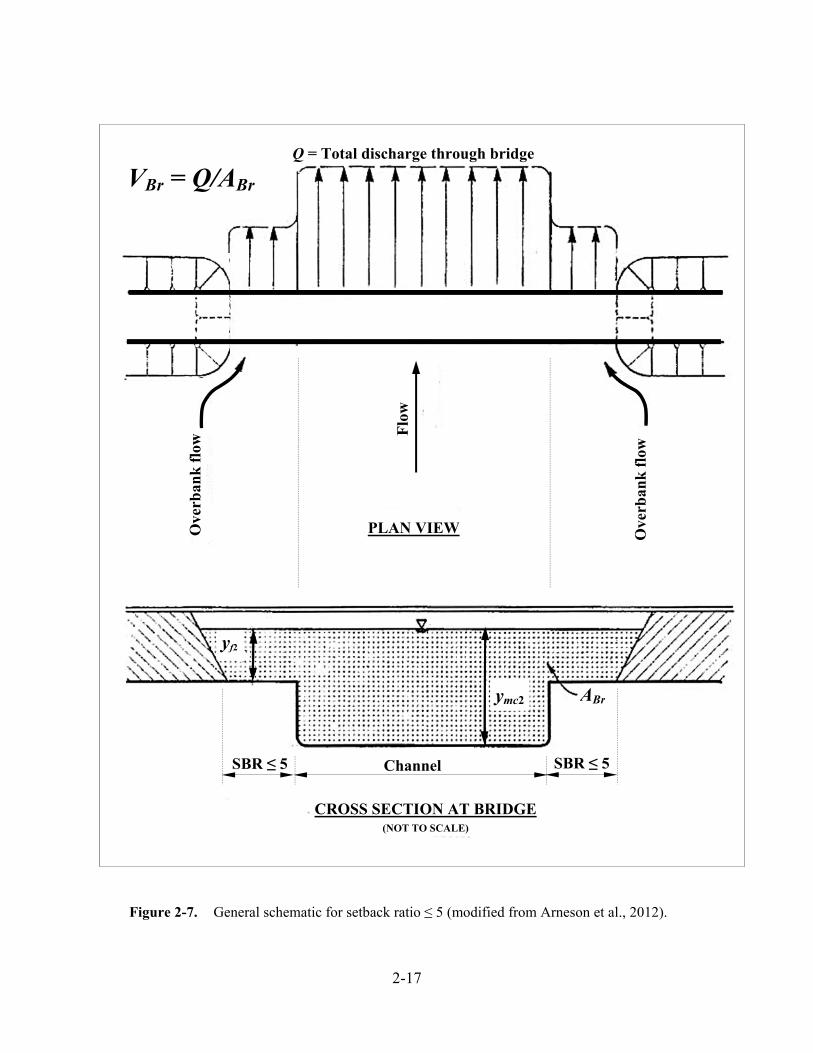
2-17
Figure 2-7. General schematic for setback ratio ≤ 5 (modified from Arneson et al., 2012).
Q = Total discharge through bridge
PLAN VIEW
VBr = Q/ABr O
verb
ank
flo
w
Ove
rban
k f
low
Flo
w
SBR ≤ 5 Channel
yf2
ymc2
CROSS SECTION AT BRIDGE (NOT TO SCALE)
SBR ≤ 5
ABr
2-18
Most of the Maine and NBSD data are represented by the case where both the left
and right abutments are at the channel bank or protrude into the channel so that
there is neither a left or right overbank at the bridge. For this case, the average
flow velocity in the bridge, VBr, was used in equation 2-8 to determine qmc2.
Additionally, for this case, the approach unit discharge determined by equation 2-
6 was used to represent the unit discharge, qmc1, in the approach channel. In some
cases, the channel at the bridge is larger than the approach channel, such that qmc2
is smaller than qmc1, and the unit discharge ratio, qmc2/qmc1, is less than a value of
1. This scenario can potentially lead to underprediction of contraction scour and
the amplification coefficient, producing underprediction of abutment scour. To
address this concern, the unit discharge at the bridge, qmc2, was arbitrarily
increased to force the unit discharge ratio, qmc2/qmc1, to have a value of 1.1. There
were 10 scour measurements in the USGS database (6 in Maine and 4 in the
NBSD) where both abutments were at the channel bank or protruded into the
channel, and the unit discharge ratio was less than 1. Tests on these data verified
that a unit discharge ratio set to a value of 1.1 eliminated underprediction for all
but one measurement. Therefore, this procedure was used for these 10
measurements.
An additional application adjustment was made to 3 measurements in the NBSD
data where the bridge length exceeded 350 ft and both abutments were at the
channel bank or protruded into the channel. For small bridge lengths, use of the
average flow velocity through the bridge is a reasonable value to estimate the
flow velocity near the abutment. However, as the bridge length increases, it is
probable that this average flow velocity begins to underestimate the larger flow
velocity near the abutment. Therefore, to minimize the risk of underestimating
the flow velocity at the abutment, a factor of 1.2 was applied to VBr in equation 2-
8 for the case where both abutments are at the bank or protrude into the channel
and the bridge length equals or exceeds 240 ft. The factor of 1.2 is based on
research by Hayes (1996), Briaud et al. (2009), and Ettema et al. (2010) and is
described in more detail in the following report section on relief bridges and
bridges over swamps. The bridge length of 240 ft is based on field observations
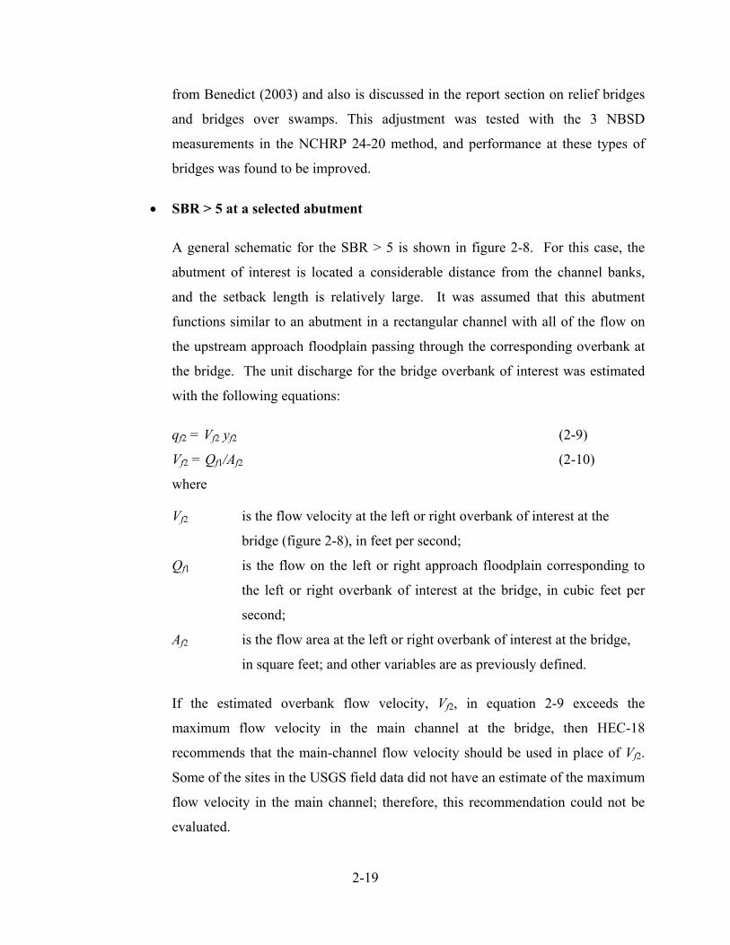
2-19
from Benedict (2003) and also is discussed in the report section on relief bridges
and bridges over swamps. This adjustment was tested with the 3 NBSD
measurements in the NCHRP 24-20 method, and performance at these types of
bridges was found to be improved.
SBR > 5 at a selected abutment
A general schematic for the SBR > 5 is shown in figure 2-8. For this case, the
abutment of interest is located a considerable distance from the channel banks,
and the setback length is relatively large. It was assumed that this abutment
functions similar to an abutment in a rectangular channel with all of the flow on
the upstream approach floodplain passing through the corresponding overbank at
the bridge. The unit discharge for the bridge overbank of interest was estimated
with the following equations:
qf2 = Vf2 yf2 (2-9)
Vf2 = Qf1/Af2 (2-10)
where
Vf2 is the flow velocity at the left or right overbank of interest at the
bridge (figure 2-8), in feet per second;
Qf1 is the flow on the left or right approach floodplain corresponding to
the left or right overbank of interest at the bridge, in cubic feet per
second;
Af2 is the flow area at the left or right overbank of interest at the bridge,
in square feet; and other variables are as previously defined.
If the estimated overbank flow velocity, Vf2, in equation 2-9 exceeds the
maximum flow velocity in the main channel at the bridge, then HEC-18
recommends that the main-channel flow velocity should be used in place of Vf2.
Some of the sites in the USGS field data did not have an estimate of the maximum
flow velocity in the main channel; therefore, this recommendation could not be
evaluated.
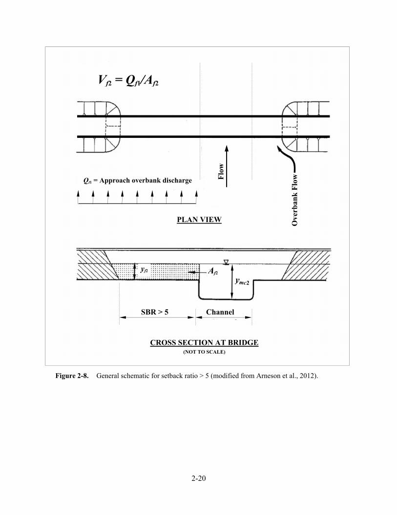
2-20
Figure 2-8. General schematic for setback ratio > 5 (modified from Arneson et al., 2012).
PLAN VIEW Ove
rban
k F
low
Flo
w
SBR > 5 Channel
CROSS SECTION AT BRIDGE (NOT TO SCALE)
Vf2 = Qf1/Af2
yf2 Af2
Qf1 = Approach overbank discharge

2-21
SBR ≤ 5 at abutment of interest and SBR > 5 at other abutment
A general schematic for the SBR > 5 is shown in figure 2-9. For this case, the
setback length for the abutment of interest is relatively small, but relatively large
at the other abutment. The average flow velocity for the abutment with an SBR ≤
5 is determined by assuming the flow on the upstream approach floodplain
associated with the abutment and flow in the approach main channel pass through
the corresponding overbank and main-channel flow area at the bridge. The unit
discharge for the abutment of interest (SBR ≤ 5) and main channel can be
determined with the following equations:
qf2 = [(Qf1+Qmc1)/(Af2+Amc2)] yf2 (2-11)
qmc2 = [(Qf1+Qmc1)/( Af2+Amc2)]ymc2 (2-12)
where
Amc2 is the flow area in the main channel at the bridge, in square feet,
with other variables as previously defined.
2-22
Figure 2-9. General schematic for setback ratio > 5 and ≤ 5 (modified from Arneson et al., 2012).
PLAN VIEW
Vf2 = (Qmc1 + Qf1)/(Af2 + Amc2)
SBR > 5 Channel
yf2ymc2
CROSS SECTION AT BRIDGE (NOT TO SCALE)
Af2 + Amc2
SBR ≤ 5
Qf1 = Approach overbank discharge
Flo
w
Qmc1 = Approach channel discharge
2-23
Relief bridge and bridge over a swamp
Special consideration must be given for application of the SBR method to a relief
bridge on a floodplain or a bridge crossing a swamp with a poorly defined
channel. In general, it was assumed that the contracted unit discharge for
abutments at relief or swamp bridges could be estimated with equation 2-7, which
assumes the average flow velocity through the bridge approximates the flow
velocity near the abutments. Based on observations by Benedict (2003), relief
and swamp bridges that are approximately 240 ft or less in length tend to form a
single scour hole across the bridge opening. This phenomenon is indicative of a
more uniform flow velocity distribution across these smaller-length bridges,
providing some support for the use of equation 2-7. However, as bridge length
increases, the assumption that the average flow velocity through the bridge
approximates the flow velocity near the abutments will become less valid. One
way to address this concern is to apply a multiplier to the average bridge velocity,
VBr, in equation 2-7 that will approximate the increased flow velocity near the
abutment. Hayes (1996) analyzed 579 streamflow measurements at gages
located at bridges in Delaware, Maryland, and Virginia and found that the
maximum point flow velocity in the bridge opening, on average, was 1.19 times
the mean flow velocity at the bridge. The Hayes (1996) relation is limited to
average flow velocities at the bridge of 10 feet per second (ft/s) or less. [Note:
Hayes (1996) added a value of 2.64 ft/s to the relation to form an envelope of the
data. For purposes of this study, the average value was considered most
appropriate, rather than the envelope values.] In support of the Hayes (1996)
observation, Briaud et al. (2009) found in laboratory data that the maximum flow
velocity near the abutment ranged from 1.04 to 1.17 times the average flow
velocity through the bridge opening. Similarly, Ettema et al. (2010) found in two-
dimensional flow models that the maximum flow velocity near the abutment
ranged from slightly greater than 1 to approximately 1.2 times the average flow
velocity through the bridge opening. (Note: The work of Morales and Ettema
(2013) provides relations for estimating the maximum flow velocity and unit
discharge at spill-through abutments with respect to selected abutment and

2-24
channel configurations, and these relations may be useful for assessing the
velocity near an abutment.) Based on these findings, it would seem reasonable to
add a multiplier of 1.2 to VBr in equation 2-7, to conservatively approximate the
increased velocity at an abutment for relief and swamp bridges. This procedure
was used at all relief and swamp bridges, with bridge lengths equaling or
exceeding 240 ft. This procedure was tested with the USGS field data in the
NCHRP 24-20 method, and performance at such bridges was improved. (Note:
This adjustment method only was applied to the field data because of its
dependence on bridge length.)
Laboratory data
For Palaviccini (1993) laboratory data with rectangular channels, the contraction
was treated like a relief bridge, as described previously, and equation 2-7 was
used to determine unit discharge through the contraction, with no adjustments.
The flow depth at the contraction, yf2, was not published in the Palaviccini (1993)
data; therefore, the approach flow depth was used to represent this value. Sturm
(2004) published the flow velocity and depth at the abutment, and these values
were used in equation 2-9 to determine unit discharge at the abutment. Ettema et
al. (2010) published the unit discharge at the abutment, and no computation was
required.
5. Calculate contraction-scour flow depth (YC)
Generally, there are two cases for contraction-scour computations: (1) abutments located
on the floodplain (setback abutments and swamps or relief bridges), and (2) abutments
located at the channel bank or protruding into the channel. A brief description of each
case follows. This approach was used in the analysis for the laboratory and field data.
2-25
Abutments located on the floodplain (setback abutments and swamp or relief
bridges)
As a general rule, NCHRP 24-20 assumes that clear-water scour conditions will
prevail on the floodplain. This is a reasonable assumption for the USGS field
data where the floodplains typically have lower velocities and are covered with
vegetation. Therefore, for setback abutments and relief and swamp bridges,
equation 2-4 was used to estimate the clear-water contraction-scour flow depth,
YC, at the abutment. For this case, the overbank unit discharge, qf2 as determined
in step 4, was used to represent the contracted unit discharge, q2, in equation 2-4.
Because the South Carolina and Alabama data primarily consist of setback
abutments or relief and swamp bridges located on vegetated floodplains, clear-
water contraction scour was assumed at all these sites.
Abutments located at the channel bank or protruding into the channel
When an abutment was located at the channel bank or protruded into the channel,
it was assumed that the prevailing sediment transport conditions within the
channel would determine the type of scour at the abutment. To determine if clear-
water or live-bed contraction-scour conditions prevailed, the average velocity in
the channel was compared with the critical velocity of the median grain size.
When live-bed scour conditions prevailed, equation 2-3 was used to estimate the
contraction-scour flow depth, YC. For this case, the unit discharge in the
approach channel, qmc1 as determined in step 3, was used to represent the
unconstricted unit discharge, q1. Similarly, the unit discharge in the bridge
channel, qmc2 as determined in step 4, was used to represent the contracted unit
discharge, q2. When clear-water scour conditions prevailed, equation 2-4 was
used to estimate the contraction-scour flow depth, YC. For this case, the unit
discharge in the bridge channel, qmc2 as determined in step 4, was used to
represent the contracted unit discharge, q2. For channels with coarse sediments in
which a critical-velocity analysis indicates that live-bed conditions prevail, HEC-
18 recommends that both live-bed and clear-water contraction-scour flow depths
2-26
be computed and the smaller of these values used as the estimate for contraction
scour. (Note: It was assumed that sediments with a D50 greater than 2 mm were
coarse sediments.) Because the USGS Maine data primarily consist of protruding
abutments into channels with coarse sediments, the smaller of the live-bed and
clear-water contraction-scour estimates was used at these sites when live-bed
scour conditions exist.
6. Determination of the amplification coefficient
Using the Scour Condition A or B as determined in step 2, the unit discharge ratio (q2/q1),
and the general abutment shape (spill through or wing wall), the appropriate graph from
figures 2-3 through 2-6 was selected, and the amplification factor, , was determined. In
order to incorporate the selection of into a spreadsheet algorithm, the solid curves for
each figure were discretized and broken into segments, and polynomial trend lines were
developed for each segment. At field sites where the unit discharge ratio, q2/q1, exceeded
the maximum value of the curves (3 for Scour Condition A and 5 for Scour Condition B),
was set to the value associated with the maximum value of q2/q1 for the given curve.
7. Calculation of abutment-scour flow depth (YMAX) and scour-hole depth (ys)
The values YC and , as determined in steps 5 and 6, respectively, were applied to
equation 2-1 to estimate the maximum flow depth in the abutment scour area (YMAX).
Equation 2-2 was then used to estimate the scour-hole depth (ys). The upstream flow
depth prior to scour, y1, as used in equation 2-2 was determined in the following manner
as for the same abutment configurations in step 5. This approach was used for laboratory
and field data.
Abutments located on the floodplain (setback abutments and swamp or relief
bridges)
The upstream flow depth prior to scour, y1, was determined from the average flow
depth on the left or right upstream approach floodplain associated with the
abutment of interest.

2-27
Abutments located at the channel bank or protruding into the channel
The upstream flow depth prior to scour, y1, was determined from the average flow
depth in the upstream approach channel.
3-1
CHAPTER 3
APPLICATION OF THE NCHRP 24-20 PREDICTION METHOD
TO LABORATORY AND FIELD DATA
3.1 Introduction
The conceptual model for the NCHRP 24-20 abutment-scour prediction method assumes that
abutment scour is a function of contraction scour. This conceptual model can be applied to
cohesive and non-cohesive sediments by incorporating an appropriate equation for predicting
contraction scour for those respective sediments. However, the current formulation of the
NCHRP 24-20 method uses the Laursen (1960; 1963) live-bed and clear-water contraction-scour
equations, which are primarily applicable to scour in non-cohesive sediments (Ettema et al.
2010; Arneson et al. 2012). A unique feature of the NCHRP 24-20 investigation was the
incorporation of laboratory data reflecting a variety of erodible and non-erodible embankments
and abutment substructures, rather than the more common fixed (or rigid) embankments and
abutments having vertical wall substructures at the abutment toe. These models better represent
embankments and abutment substructures for many field sites and will tend to reduce the
potential for abutment scour in contrast to the rigid embankment and abutment substructures
used in previous studies. The current (2015) investigation will only evaluate the NCHRP 24-20
method for Scour Condition A, where an abutment is set near the main channel, and Scour
Condition B, where the abutment is well set back from the main channel. Because of the
complexity of flow and scour patterns for Scour Condition A, NCHRP 24-20 developed scour
prediction methods based on data from the fixed floodplain and abutment models, providing a
more conservative estimate of abutment scour. For Scour Condition B, NCHRP 24-20 developed
scour prediction methods based on data from erodible floodplain and abutment substructures,
with the embankment and abutment armored with rip rap. (See report section 2.2 for more details
regarding the abutment models used in the NCHRP 24-20 investigation.)
With the exception of the NCHRP 24-20 laboratory data, the laboratory data used in evaluating
the performance of the NCHRP 24-20 prediction method represent scour at non-erodible rigid
3-2
embankments, abutments, and abutment substructures. Additionally, the conditions of the
embankments/abutments for the USGS field data are thought to represent abutment scour where
the road embankment and abutments did not appreciably erode (see report section 1.2.5 for
details). These characteristics of the laboratory and field data differ in some measure from the
abutment models used in the NCHRP 24-20 investigation (see report section 2.2). These
differences should be kept in mind when reviewing the results of the NCHRP 24-20 prediction
method presented in this report.
The procedure described in chapter 2 was used to apply the NCHRP 24-20 abutment-scour
prediction method to the selected laboratory (table 1-3) and field (table 1-1) abutment-scour data.
The results from this application were incorporated into selected scatter plots to display the
relations of predicted and measured scour, as well as prediction residuals with respect to selected
explanatory variables. If a prediction equation is capturing the trends of the data, then the
relation of the predicted and measured scour will tend to follow the line of agreement, with
predicted scour increasing as measured scour increases. The relation of prediction residuals with
respect to an explanatory variable will help identify prediction bias associated with that variable.
If prediction residuals display a sloped trend with respect to a given explanatory variable, some
prediction bias with respect to that variable is likely. Boxplots of the prediction residuals for the
laboratory and field data are presented in chapter 6 and compared with the prediction residuals of
the NCHRP 24-15(2) method. The boxplots display the distribution of the prediction residuals
by quartiles, providing a simple but useful tool for evaluating the performance of each method
and comparing their performance. A table of summary statistics for these boxplots also is
provided in chapter 6 in order to quantify the trends in the boxplots.
The performance of the NCHRP 24-20 prediction method presented in the following sections of
this report represents the combined influence of the equation, the prescribed application
procedure, and the data, each having inherent limitations. These limitations will undoubtedly
introduce uncertainty into the results; however, the large number of laboratory (table 1-3) and
field (table 1-1) data should be adequate to provide valuable insights into the general
performance of the equation. The results associated with the laboratory data will be presented
first followed by the results of the field data.
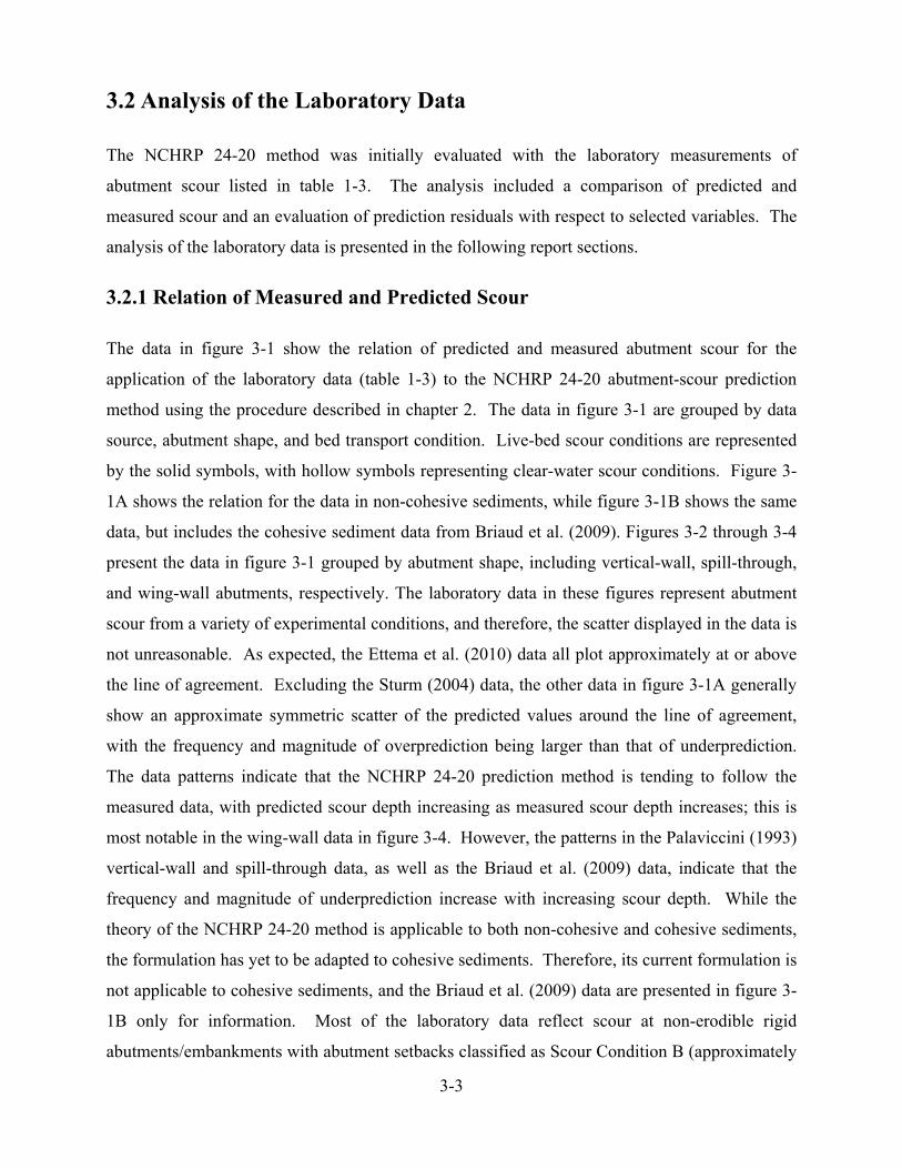
3-3
3.2 Analysis of the Laboratory Data
The NCHRP 24-20 method was initially evaluated with the laboratory measurements of
abutment scour listed in table 1-3. The analysis included a comparison of predicted and
measured scour and an evaluation of prediction residuals with respect to selected variables. The
analysis of the laboratory data is presented in the following report sections.
3.2.1 Relation of Measured and Predicted Scour
The data in figure 3-1 show the relation of predicted and measured abutment scour for the
application of the laboratory data (table 1-3) to the NCHRP 24-20 abutment-scour prediction
method using the procedure described in chapter 2. The data in figure 3-1 are grouped by data
source, abutment shape, and bed transport condition. Live-bed scour conditions are represented
by the solid symbols, with hollow symbols representing clear-water scour conditions. Figure 3-
1A shows the relation for the data in non-cohesive sediments, while figure 3-1B shows the same
data, but includes the cohesive sediment data from Briaud et al. (2009). Figures 3-2 through 3-4
present the data in figure 3-1 grouped by abutment shape, including vertical-wall, spill-through,
and wing-wall abutments, respectively. The laboratory data in these figures represent abutment
scour from a variety of experimental conditions, and therefore, the scatter displayed in the data is
not unreasonable. As expected, the Ettema et al. (2010) data all plot approximately at or above
the line of agreement. Excluding the Sturm (2004) data, the other data in figure 3-1A generally
show an approximate symmetric scatter of the predicted values around the line of agreement,
with the frequency and magnitude of overprediction being larger than that of underprediction.
The data patterns indicate that the NCHRP 24-20 prediction method is tending to follow the
measured data, with predicted scour depth increasing as measured scour depth increases; this is
most notable in the wing-wall data in figure 3-4. However, the patterns in the Palaviccini (1993)
vertical-wall and spill-through data, as well as the Briaud et al. (2009) data, indicate that the
frequency and magnitude of underprediction increase with increasing scour depth. While the
theory of the NCHRP 24-20 method is applicable to both non-cohesive and cohesive sediments,
the formulation has yet to be adapted to cohesive sediments. Therefore, its current formulation is
not applicable to cohesive sediments, and the Briaud et al. (2009) data are presented in figure 3-
1B only for information. Most of the laboratory data reflect scour at non-erodible rigid
abutments/embankments with abutment setbacks classified as Scour Condition B (approximately
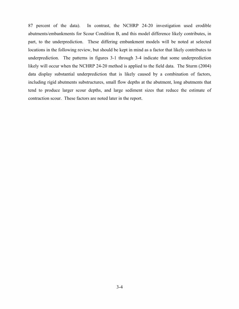
3-4
87 percent of the data). In contrast, the NCHRP 24-20 investigation used erodible
abutments/embankments for Scour Condition B, and this model difference likely contributes, in
part, to the underprediction. These differing embankment models will be noted at selected
locations in the following review, but should be kept in mind as a factor that likely contributes to
underprediction. The patterns in figures 3-1 through 3-4 indicate that some underprediction
likely will occur when the NCHRP 24-20 method is applied to the field data. The Sturm (2004)
data display substantial underprediction that is likely caused by a combination of factors,
including rigid abutments substructures, small flow depths at the abutment, long abutments that
tend to produce larger scour depths, and large sediment sizes that reduce the estimate of
contraction scour. These factors are noted later in the report.
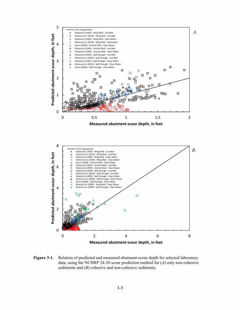
3-5
Figure 3-1. Relation of predicted and measured abutment-scour depth for selected laboratory
data, using the NCHRP 24-20 scour prediction method for (A) only non-cohesive sediments and (B) cohesive and non-cohesive sediments.
0
2
4
6
8
0 2 4 6 8
Predicted abutm
ent‐scour depth, in feet
Measured abutment‐scour depth, in feet
Line of agreementPalaviccini (1993) ‐ Wing Wall ‐ Live BedEttema et al. (2010) ‐ Wing Wall ‐ Live BedPalaviccini (1993) ‐ Wing Wall ‐ Clear WaterEttema et al. (2010) ‐ Wing Wall ‐ Clear WaterSturm (2004) ‐ Vertical Wall ‐ Clear WaterPalaviccini (1993) ‐ Vertical Wall ‐ Live BedPalaviccini (1993) ‐ Vertical Wall ‐ Clear WaterPalaviccini (1993) ‐ Spill through ‐ Live BedEttema et al. (2010) ‐ Spill through ‐ Live BedPalaviccini (1993) ‐ Spill through ‐ Clear WaterEttema et al. (2010) ‐ Spill through ‐ Clear WaterSturm (2004) ‐ Spill through ‐ Clear WaterBriaud et al. (2009) ‐ Wing Wall ‐ Clear WaterBriaud et al. (2009) ‐ Spill through ‐ Clear Water
0
1
2
3
4
5
0 0.5 1 1.5 2
Predicted abutm
ent‐scour depth, in feet
Measured abutment‐scour depth, in feet
Line of agreement
Palaviccini (1993) ‐ Wing Wall ‐ Live Bed
Ettema et al. (2010) ‐ Wing Wall ‐ Live Bed
Palaviccini (1993) ‐ Wing Wall ‐ Clear Water
Ettema et al. (2010) ‐ Wing Wall ‐ Clearwater
Sturm (2004) ‐ Vertical Wall ‐ Clear Water
Palaviccini (1993) ‐ Vertical Wall ‐ Live Bed
Palaviccini (1993) ‐ Vertical Wall ‐ Clear Water
Palaviccini (1993) ‐ Spill through ‐ Live Bed
Ettema et al. (2010) ‐ Spill through ‐ Live Bed
Palaviccini (1993) ‐ Spill through ‐ Clear Water
Ettema et al. (2010) ‐ Spill through ‐ Clear Water
Sturm (2004) ‐ Spill through ‐ Clear Water
A.
B.

3-6
Figure 3-2. Relation of predicted and measured abutment-scour depth for selected laboratory data with vertical-wall abutments, using the NCHRP 24-20 scour prediction method.
Figure 3-3. Relation of predicted and measured abutment-scour depth for selected laboratory data with spill-through abutments, using the NCHRP 24-20 scour prediction method.
0
1
2
3
4
0 0.5 1 1.5 2
Predicted abutm
ent‐scour depth, in feet
Measured abutment‐scour depth, in feet
Line of agreement
Palaviccini (1993) ‐ Vertical Wall ‐ Live Bed
Palaviccini (1993) ‐ Vertical Wall ‐ Clear Water
Sturm (2004) ‐ Vertical Wall ‐ Clear Water
0
1
2
3
4
0 0.5 1 1.5 2
Predicted abutm
ent‐scour depth, in feet
Measured abutment‐scour depth, in feet
Line of agreement
Palaviccini (1993) ‐ Spill through ‐ Live Bed
Palaviccini (1993) ‐ Spill through ‐ Clear Water
Sturm (2004) ‐ Spill through ‐ Clear Water
Ettema et al. (2010) ‐ Spill through ‐ Live Bed
Ettema et al. (2010) ‐ Spill through ‐ Clear Water
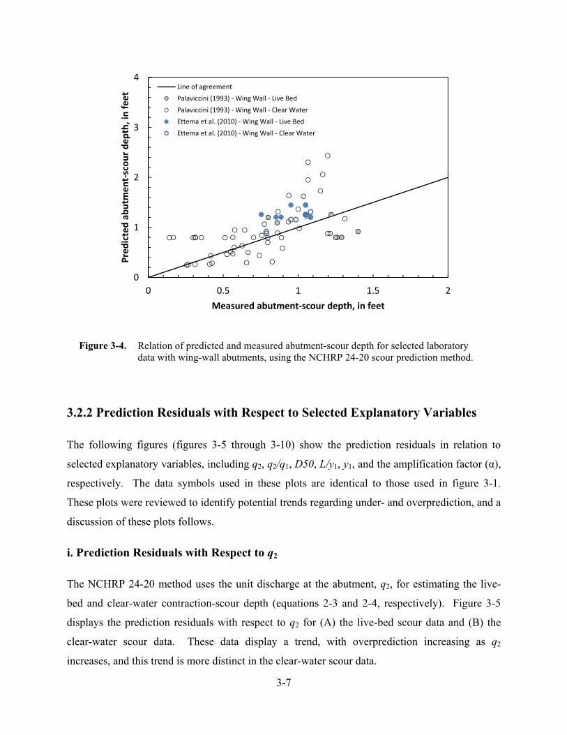
3-7
Figure 3-4. Relation of predicted and measured abutment-scour depth for selected laboratory data with wing-wall abutments, using the NCHRP 24-20 scour prediction method.
3.2.2 Prediction Residuals with Respect to Selected Explanatory Variables
The following figures (figures 3-5 through 3-10) show the prediction residuals in relation to
selected explanatory variables, including q2, q2/q1, D50, L/y1, y1, and the amplification factor (α),
respectively. The data symbols used in these plots are identical to those used in figure 3-1.
These plots were reviewed to identify potential trends regarding under- and overprediction, and a
discussion of these plots follows.
i. Prediction Residuals with Respect to q2
The NCHRP 24-20 method uses the unit discharge at the abutment, q2, for estimating the live-
bed and clear-water contraction-scour depth (equations 2-3 and 2-4, respectively). Figure 3-5
displays the prediction residuals with respect to q2 for (A) the live-bed scour data and (B) the
clear-water scour data. These data display a trend, with overprediction increasing as q2
increases, and this trend is more distinct in the clear-water scour data.
0
1
2
3
4
0 0.5 1 1.5 2
Predicted abutm
ent‐scour depth, in feet
Measured abutment‐scour depth, in feet
Line of agreement
Palaviccini (1993) ‐ Wing Wall ‐ Live Bed
Palaviccini (1993) ‐ Wing Wall ‐ Clear Water
Ettema et al. (2010) ‐ Wing Wall ‐ Live Bed
Ettema et al. (2010) ‐ Wing Wall ‐ Clear Water
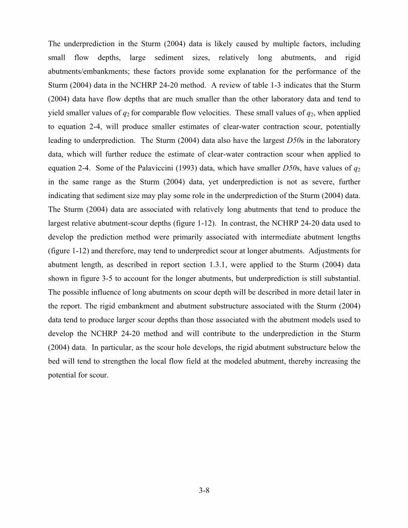
3-8
The underprediction in the Sturm (2004) data is likely caused by multiple factors, including
small flow depths, large sediment sizes, relatively long abutments, and rigid
abutments/embankments; these factors provide some explanation for the performance of the
Sturm (2004) data in the NCHRP 24-20 method. A review of table 1-3 indicates that the Sturm
(2004) data have flow depths that are much smaller than the other laboratory data and tend to
yield smaller values of q2 for comparable flow velocities. These small values of q2, when applied
to equation 2-4, will produce smaller estimates of clear-water contraction scour, potentially
leading to underprediction. The Sturm (2004) data also have the largest D50s in the laboratory
data, which will further reduce the estimate of clear-water contraction scour when applied to
equation 2-4. Some of the Palaviccini (1993) data, which have smaller D50s, have values of q2
in the same range as the Sturm (2004) data, yet underprediction is not as severe, further
indicating that sediment size may play some role in the underprediction of the Sturm (2004) data.
The Sturm (2004) data are associated with relatively long abutments that tend to produce the
largest relative abutment-scour depths (figure 1-12). In contrast, the NCHRP 24-20 data used to
develop the prediction method were primarily associated with intermediate abutment lengths
(figure 1-12) and therefore, may tend to underpredict scour at longer abutments. Adjustments for
abutment length, as described in report section 1.3.1, were applied to the Sturm (2004) data
shown in figure 3-5 to account for the longer abutments, but underprediction is still substantial.
The possible influence of long abutments on scour depth will be described in more detail later in
the report. The rigid embankment and abutment substructure associated with the Sturm (2004)
data tend to produce larger scour depths than those associated with the abutment models used to
develop the NCHRP 24-20 method and will contribute to the underprediction in the Sturm
(2004) data. In particular, as the scour hole develops, the rigid abutment substructure below the
bed will tend to strengthen the local flow field at the modeled abutment, thereby increasing the
potential for scour.
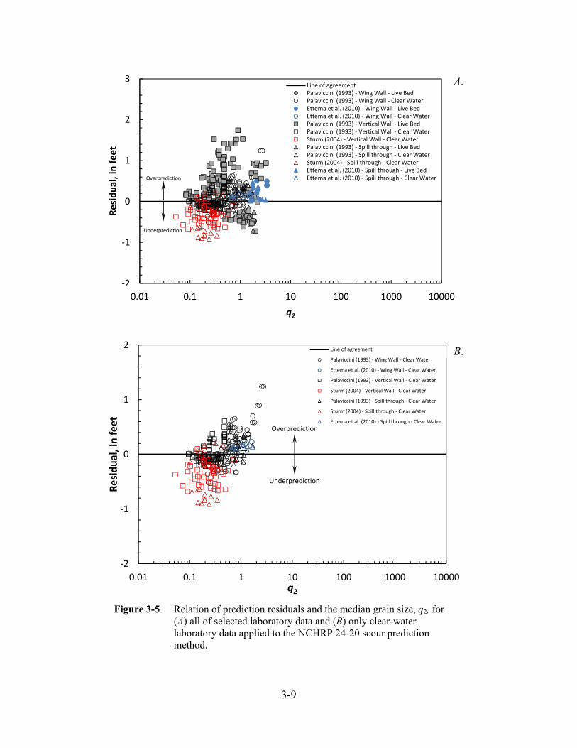
3-9
Figure 3-5. Relation of prediction residuals and the median grain size, q2, for (A) all of selected laboratory data and (B) only clear-water laboratory data applied to the NCHRP 24-20 scour prediction method.
‐2
‐1
0
1
2
0.01 0.1 1 10 100 1000 10000
Residual, in feet
q2
Line of agreement
Palaviccini (1993) ‐ Wing Wall ‐ Clear Water
Ettema et al. (2010) ‐ Wing Wall ‐ Clear Water
Palaviccini (1993) ‐ Vertical Wall ‐ Clear Water
Sturm (2004) ‐ Vertical Wall ‐ Clear Water
Palaviccini (1993) ‐ Spill through ‐ Clear Water
Sturm (2004) ‐ Spill through ‐ Clear Water
Ettema et al. (2010) ‐ Spill through ‐ Clear Water
Overprediction
Underprediction
‐2
‐1
0
1
2
3
0.01 0.1 1 10 100 1000 10000
Residual, in feet
q2
Line of agreementPalaviccini (1993) ‐ Wing Wall ‐ Live BedPalaviccini (1993) ‐ Wing Wall ‐ Clear WaterEttema et al. (2010) ‐ Wing Wall ‐ Live BedEttema et al. (2010) ‐ Wing Wall ‐ Clear WaterPalaviccini (1993) ‐ Vertical Wall ‐ Live BedPalaviccini (1993) ‐ Vertical Wall ‐ Clear WaterSturm (2004) ‐ Vertical Wall ‐ Clear WaterPalaviccini (1993) ‐ Spill through ‐ Live BedPalaviccini (1993) ‐ Spill through ‐ Clear WaterSturm (2004) ‐ Spill through ‐ Clear WaterEttema et al. (2010) ‐ Spill through ‐ Live BedEttema et al. (2010) ‐ Spill through ‐ Clear WaterOverprediction
Underprediction
A.
B.
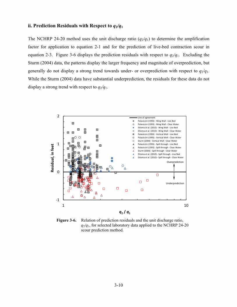
3-10
ii. Prediction Residuals with Respect to q2/q1
The NCHRP 24-20 method uses the unit discharge ratio (q2/q1) to determine the amplification
factor for application to equation 2-1 and for the prediction of live-bed contraction scour in
equation 2-3. Figure 3-6 displays the prediction residuals with respect to q2/q1. Excluding the
Sturm (2004) data, the patterns display the larger frequency and magnitude of overprediction, but
generally do not display a strong trend towards under- or overprediction with respect to q2/q1.
While the Sturm (2004) data have substantial underprediction, the residuals for these data do not
display a strong trend with respect to q2/q1.
‐1
0
1
2
1 10
Residual, in feet
q2 / q1
Line of agreement
Palaviccini (1993) ‐ Wing Wall ‐ Live Bed
Palaviccini (1993) ‐ Wing Wall ‐ Clear Water
Ettema et al. (2010) ‐ Wing Wall ‐ Live Bed
Ettema et al. (2010) ‐ Wing Wall ‐ Clear Water
Palaviccini (1993) ‐ Vertical Wall ‐ Live Bed
Palaviccini (1993) ‐ Vertical Wall ‐ Clear Water
Sturm (2004) ‐ Vertical Wall ‐ Clear Water
Palaviccini (1993) ‐ Spill through ‐ Live Bed
Palaviccini (1993) ‐ Spill through ‐ Clear Water
Sturm (2004) ‐ Spill through ‐ Clear Water
Ettema et al. (2010) ‐ Spill through ‐ Live Bed
Ettema et al. (2010) ‐ Spill through ‐ Clear Water
Overprediction
Underprediction
Figure 3-6. Relation of prediction residuals and the unit discharge ratio, q2/q1, for selected laboratory data applied to the NCHRP 24-20 scour prediction method.
3-11
iii. Prediction Residuals with Respect to D50
The median grain size of the sediment, D50, is used in equation 2-4 to estimate the clear-water
contraction-scour depth. Figure 3-7 shows the relation of the prediction residuals with respect to
D50 for (A) all of the laboratory data and (B) the clear-water scour data. The trend in figure 3-
7A indicates that the magnitude of overprediction diminishes with more frequent underprediction
as D50 increases. The data for clear-water scour (figure 3-7B) display a similar, but less
prominent relation. The Sturm (2004) data strongly influence the patterns in figure 3-7B, and if
they are neglected, the trend is not as prominent. As noted previously, multiple factors likely
contribute to the underprediction associated with the Sturm (2004) data, with sediment size being
one of these factors.
iv. Prediction Residuals with Respect to L/y1
The relative abutment length, L/y1, is a variable used by Melville and Coleman (2000) to classify
abutments into categories of short, intermediate, and long abutments, with the potential for
abutment-scour increasing as the abutment length increases (report section 1.3.2 and figure 1-
12). The relation of the prediction residuals with respect to L/y1 is shown in figure 3-8 for (A) all
of the laboratory data and (B) the clear-water scour data. The figure identifies the range for
short, intermediate, and long abutments as classified by Melville and Coleman (2000). The data
indicate a trend of overprediction associated with shorter abutments and underprediction
associated with longer abutments. If the Sturm (2004) data are neglected, the trend is still
prominent, indicating that L/y1 likely has some influence on residual patterns and that
underprediction will tend to be associated with clear-water scour at relatively long abutments.
Because a large number of the USGS field data are classified as clear-water scour with relatively
long abutments, figure 3-8B provides some insight on how such field data may perform with the
NCHRP 24-20 method.
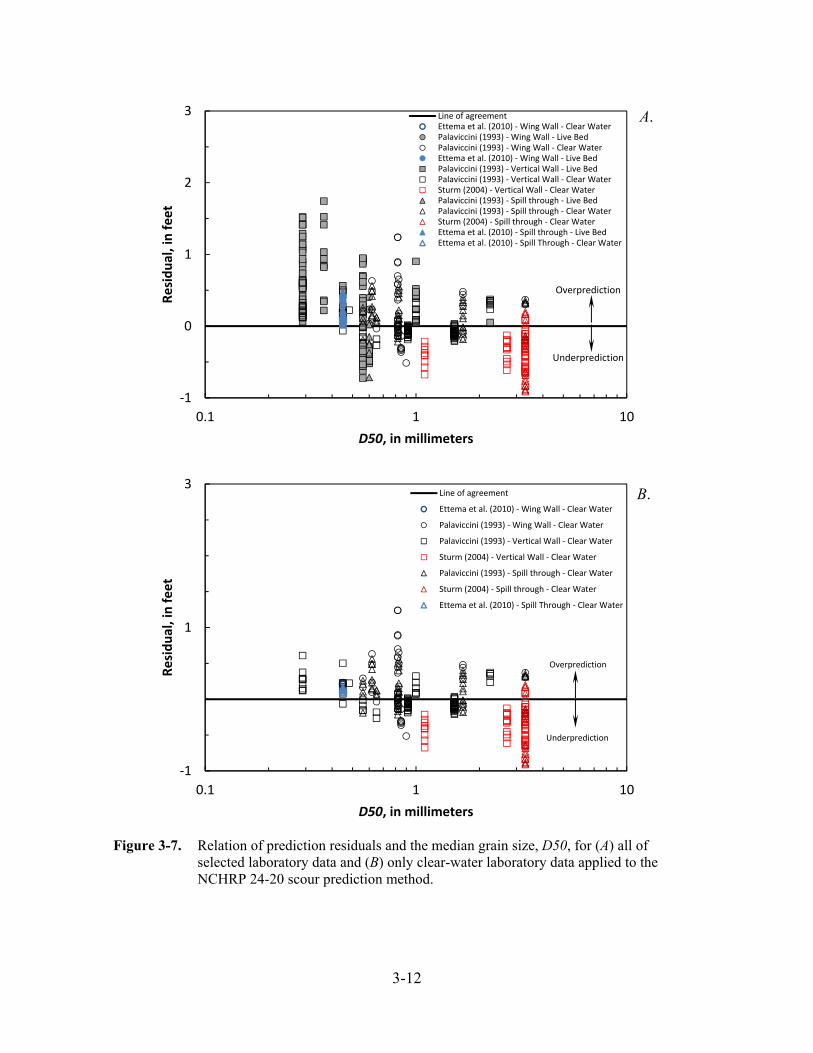
3-12
Figure 3-7. Relation of prediction residuals and the median grain size, D50, for (A) all of selected laboratory data and (B) only clear-water laboratory data applied to the NCHRP 24-20 scour prediction method.
‐1
1
3
0.1 1 10
Residual, in feet
D50, in millimeters
Line of agreement
Ettema et al. (2010) ‐ Wing Wall ‐ Clear Water
Palaviccini (1993) ‐ Wing Wall ‐ Clear Water
Palaviccini (1993) ‐ Vertical Wall ‐ Clear Water
Sturm (2004) ‐ Vertical Wall ‐ Clear Water
Palaviccini (1993) ‐ Spill through ‐ Clear Water
Sturm (2004) ‐ Spill through ‐ Clear Water
Ettema et al. (2010) ‐ Spill Through ‐ Clear Water
Overprediction
Underprediction
‐1
0
1
2
3
0.1 1 10
Residual, in feet
D50, in millimeters
Line of agreementEttema et al. (2010) ‐ Wing Wall ‐ Clear WaterPalaviccini (1993) ‐ Wing Wall ‐ Live BedPalaviccini (1993) ‐ Wing Wall ‐ Clear WaterEttema et al. (2010) ‐ Wing Wall ‐ Live BedPalaviccini (1993) ‐ Vertical Wall ‐ Live BedPalaviccini (1993) ‐ Vertical Wall ‐ Clear WaterSturm (2004) ‐ Vertical Wall ‐ Clear WaterPalaviccini (1993) ‐ Spill through ‐ Live BedPalaviccini (1993) ‐ Spill through ‐ Clear WaterSturm (2004) ‐ Spill through ‐ Clear WaterEttema et al. (2010) ‐ Spill through ‐ Live BedEttema et al. (2010) ‐ Spill Through ‐ Clear Water
Overprediction
Underprediction
A.
B.
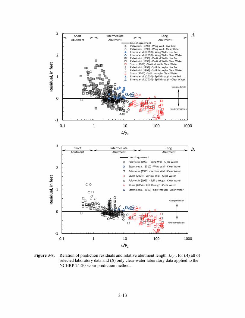
3-13
Figure 3-8. Relation of prediction residuals and relative abutment length, L/y1, for (A) all of selected laboratory data and (B) only clear-water laboratory data applied to the NCHRP 24-20 scour prediction method.
‐1
0
1
2
3
0.1 1 10 100 1000
Residual, in feet
L/y1
Line of agreement
Palaviccini (1993) ‐ Wing Wall ‐ Clear Water
Ettema et al. (2010) ‐ Wing Wall ‐ Clear Water
Palaviccini (1993) ‐ Vertical Wall ‐ Clear Water
Sturm (2004) ‐ Vertical Wall ‐ Clear Water
Palaviccini (1993) ‐ Spill through ‐ Clear Water
Sturm (2004) ‐ Spill through ‐ Clear Water
Ettema et al. (2010) ‐ Spill through ‐ Clear Water
Long Abutment
IntermediateAbutment
ShortAbutment
Overprediction
Underprediction
‐1
0
1
2
3
0.1 1 10 100 1000
Residual, in feet
L/y1
Line of agreementPalaviccini (1993) ‐ Wing Wall ‐ Live BedPalaviccini (1993) ‐ Wing Wall ‐ Clear WaterEttema et al. (2010) ‐ Wing Wall ‐ Live BedEttema et al. (2010) ‐ Wing Wall ‐ Clear WaterPalaviccini (1993) ‐ Vertical Wall ‐ Live BedPalaviccini (1993) ‐ Vertical Wall ‐ Clear WaterSturm (2004) ‐ Vertical Wall ‐ Clear WaterPalaviccini (1993) ‐ Spill through ‐ Live BedPalaviccini (1993) ‐ Spill through ‐ Clear WaterSturm (2004) ‐ Spill through ‐ Clear WaterEttema et al. (2010) ‐ Spill through ‐ Live BedEttema et al. (2010) ‐ Spill through ‐ Clear Water
Long Abutment
IntermediateAbutment
ShortAbutment
Overprediction
Underprediction
A.
B.
3-14
v. Prediction Residuals with Respect to y1
The approach flow depth, y1, is a variable used directly or indirectly in equations 2-2 through 2-4
for predicting abutment scour. The relation of the prediction residuals with respect to y1 is shown
in figure 3-9 for (A) all of the laboratory data and (B) the clear-water scour data. There is a
relation associated with these data, with the frequency and magnitude of overprediction
increasing as y1 increases. Underprediction is associated with small flow depths and provides
some explanation for the differing performance of the Sturm (2004) data, which have the
smallest values of y1 within the laboratory data.
vi. Prediction Residuals with Respect to α
The amplification factor, which is used in equation 2-1, accounts for the additional scour at an
abutment that is above and beyond the contraction scour. The relation of the prediction residuals
with respect to the amplification factor is shown in figure 3-10 for (A) all of the laboratory data
and (B) the clear-water scour data without the Sturm (2004) data. For amplification factors
greater than 2, there is more frequent overprediction, but no strong trend in the residuals. The
Sturm (2004) data indicate a tendency for increased underprediction as the amplification factor
decreases, but the trend is not strong and is likely influenced by other factors as noted previously.
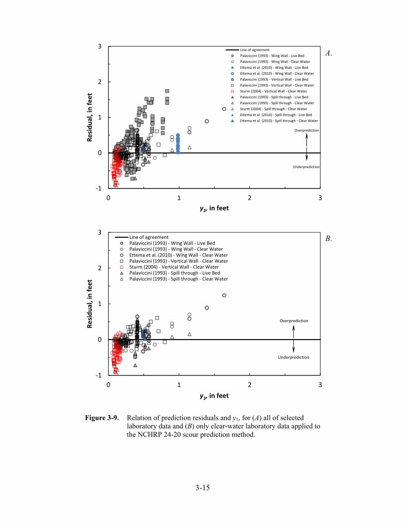
3-15
Figure 3-9. Relation of prediction residuals and y1, for (A) all of selected
laboratory data and (B) only clear-water laboratory data applied to the NCHRP 24-20 scour prediction method.
‐1
0
1
2
3
0 1 2 3
Residual, in feet
y1, in feet
Line of agreementPalaviccini (1993) ‐ Wing Wall ‐ Live BedPalaviccini (1993) ‐ Wing Wall ‐ Clear WaterEttema et al. (2010) ‐ Wing Wall ‐ Clear WaterPalaviccini (1993) ‐ Vertical Wall ‐ Clear WaterSturm (2004) ‐ Vertical Wall ‐ Clear WaterPalaviccini (1993) ‐ Spill through ‐ Live BedPalaviccini (1993) ‐ Spill through ‐ Clear Water
Overprediction
Underprediction
‐1
0
1
2
3
0 1 2 3
Residual, in feet
y1, in feet
Line of agreement
Palaviccini (1993) ‐ Wing Wall ‐ Live Bed
Palaviccini (1993) ‐ Wing Wall ‐ Clear Water
Ettema et al. (2010) ‐ Wing Wall ‐ Live Bed
Ettema et al. (2010) ‐ Wing Wall ‐ Clear Water
Palaviccini (1993) ‐ Vertical Wall ‐ Live Bed
Palaviccini (1993) ‐ Vertical Wall ‐ Clear Water
Sturm (2004) ‐ Vertical Wall ‐ Clear Water
Palaviccini (1993) ‐ Spill through ‐ Live Bed
Palaviccini (1993) ‐ Spill through ‐ Clear Water
Sturm (2004) ‐ Spill through ‐ Clear Water
Ettema et al. (2010) ‐ Spill through ‐ Live Bed
Ettema et al. (2010) ‐ Spill through ‐ Clear Water
Overprediction
Underprediction
A.
B.
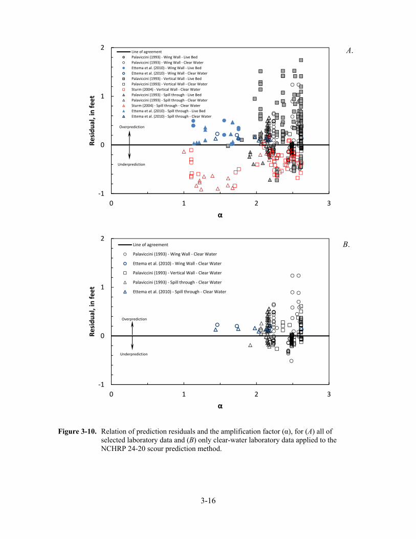
3-16
Figure 3-10. Relation of prediction residuals and the amplification factor (α), for (A) all of
selected laboratory data and (B) only clear-water laboratory data applied to the NCHRP 24-20 scour prediction method.
A.
B.
‐1
0
1
2
0 1 2 3
Residual, in feet
α
Line of agreement
Palaviccini (1993) ‐ Wing Wall ‐ Live Bed
Palaviccini (1993) ‐ Wing Wall ‐ Clear Water
Ettema et al. (2010) ‐ Wing Wall ‐ Live Bed
Ettema et al. (2010) ‐ Wing Wall ‐ Clear Water
Palaviccini (1993) ‐ Vertical Wall ‐ Live Bed
Palaviccini (1993) ‐ Vertical Wall ‐ Clear Water
Sturm (2004) ‐ Vertical Wall ‐ Clear Water
Palaviccini (1993) ‐ Spill through ‐ Live Bed
Palaviccini (1993) ‐ Spill through ‐ Clear Water
Sturm (2004) ‐ Spill through ‐ Clear Water
Ettema et al. (2010) ‐ Spill through ‐ Live Bed
Ettema et al. (2010) ‐ Spill through ‐ Clear Water
Overprediction
Underprediction
‐1
0
1
2
0 1 2 3
Residual, in feet
α
Line of agreement
Palaviccini (1993) ‐ Wing Wall ‐ Clear Water
Ettema et al. (2010) ‐ Wing Wall ‐ Clear Water
Palaviccini (1993) ‐ Vertical Wall ‐ Clear Water
Palaviccini (1993) ‐ Spill through ‐ Clear Water
Ettema et al. (2010) ‐ Spill through ‐ Clear Water
Overprediction
Underprediction
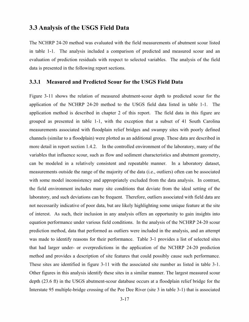
3-17
3.3 Analysis of the USGS Field Data
The NCHRP 24-20 method was evaluated with the field measurements of abutment scour listed
in table 1-1. The analysis included a comparison of predicted and measured scour and an
evaluation of prediction residuals with respect to selected variables. The analysis of the field
data is presented in the following report sections.
3.3.1 Measured and Predicted Scour for the USGS Field Data
Figure 3-11 shows the relation of measured abutment-scour depth to predicted scour for the
application of the NCHRP 24-20 method to the USGS field data listed in table 1-1. The
application method is described in chapter 2 of this report. The field data in this figure are
grouped as presented in table 1-1, with the exception that a subset of 41 South Carolina
measurements associated with floodplain relief bridges and swampy sites with poorly defined
channels (similar to a floodplain) were plotted as an additional group. These data are described in
more detail in report section 1.4.2. In the controlled environment of the laboratory, many of the
variables that influence scour, such as flow and sediment characteristics and abutment geometry,
can be modeled in a relatively consistent and repeatable manner. In a laboratory dataset,
measurements outside the range of the majority of the data (i.e., outliers) often can be associated
with some model inconsistency and appropriately excluded from the data analysis. In contrast,
the field environment includes many site conditions that deviate from the ideal setting of the
laboratory, and such deviations can be frequent. Therefore, outliers associated with field data are
not necessarily indicative of poor data, but are likely highlighting some unique feature at the site
of interest. As such, their inclusion in any analysis offers an opportunity to gain insights into
equation performance under various field conditions. In the analysis of the NCHRP 24-20 scour
prediction method, data that performed as outliers were included in the analysis, and an attempt
was made to identify reasons for their performance. Table 3-1 provides a list of selected sites
that had larger under- or overpredictions in the application of the NCHRP 24-20 prediction
method and provides a description of site features that could possibly cause such performance.
These sites are identified in figure 3-11 with the associated site number as listed in table 3-1.
Other figures in this analysis identify these sites in a similar manner. The largest measured scour
depth (23.6 ft) in the USGS abutment-scour database occurs at a floodplain relief bridge for the
Interstate 95 multiple-bridge crossing of the Pee Dee River (site 3 in table 3-1) that is associated
3-18
with an approximately 8-mile-wide floodplain. The one-dimensional model for this site
indicates a large water-surface differential (backwater) of approximately 2 ft across the bridge,
which creates hydraulic conditions that can have a large potential for scour. Because of these
adverse hydraulic conditions, this site likely will perform poorly with most laboratory-derived
scour prediction equations that typically would not include data for such severe hydraulic
conditions. Additionally, the one-dimensional flow model for this site will not fully capture the
hydraulics, introducing some error in any scour analysis. This data point was included in the
analysis to provide perspective of how the selected equation will perform under more severe
scour conditions.
To better visualize the trends in figure 3-11, the data points associated with each data group are
shown in figure 3-12 as a series of plots. All of the field data are shown as hollow circles, with
the selected data group identified with solid circles. The lower gradient and wide floodplain
streams associated with the South Carolina Relief/Swamp Bridges and the Coastal Plain are
shown in figures 3-12A and B, respectively. The larger outliers associated with these data
groups have site features that provide some explanation for their performance (table 3-1).
Excluding the data in table 3-1, the data generally show an approximate symmetric scatter of the
predicted values around the line of agreement, with the frequency and magnitude of
overprediction being larger than that for underprediction. However, as with the laboratory data
(figure 3-1), there is a trend of more frequent underprediction as the scour depth increases. In
particular, there is more frequent underprediction of scour for measured abutment-scour depths
of approximately 10 ft and larger. The underprediction in these data likely is caused by multiple
factors, some of which include (1) relatively long abutments that tend to produce larger scour
depths in contrast to the intermediate abutments used to develop the NCHRP 24-20 method (see
report section 1.3.1), (2) the less accurate estimates of flow velocity from the one-dimensional
flow models, and (3) relatively non-erodible abutments/embankments in contrast to the erodible
abutments/embankments used to develop the NCHRP 24-20 prediction method (see report
section 1.2.5). Note that 23 of the 29 underpredictions from these two data groups are associated
with Scour Condition B, where the NCHRP 24-20 method assumes erodible embankments and
abutments, giving some support to item 3 in the previous sentence. For the cohesive sediments of
the South Carolina Piedmont and Alabama (figures 3-12C and E), the data pattern indicates a
higher occurrence of overprediction with infrequent underprediction. Because the current
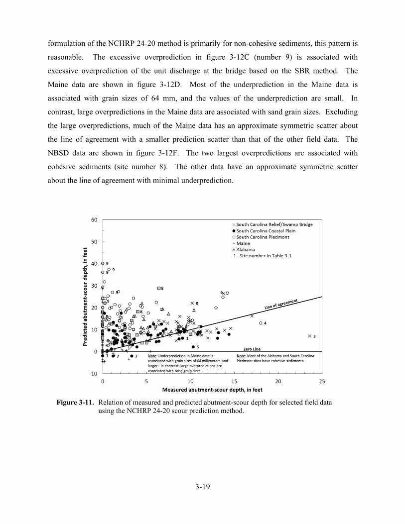
3-19
formulation of the NCHRP 24-20 method is primarily for non-cohesive sediments, this pattern is
reasonable. The excessive overprediction in figure 3-12C (number 9) is associated with
excessive overprediction of the unit discharge at the bridge based on the SBR method. The
Maine data are shown in figure 3-12D. Most of the underprediction in the Maine data is
associated with grain sizes of 64 mm, and the values of the underprediction are small. In
contrast, large overpredictions in the Maine data are associated with sand grain sizes. Excluding
the large overpredictions, much of the Maine data has an approximate symmetric scatter about
the line of agreement with a smaller prediction scatter than that of the other field data. The
NBSD data are shown in figure 3-12F. The two largest overpredictions are associated with
cohesive sediments (site number 8). The other data have an approximate symmetric scatter
about the line of agreement with minimal underprediction.
Figure 3-11. Relation of measured and predicted abutment-scour depth for selected field data using the NCHRP 24-20 scour prediction method.
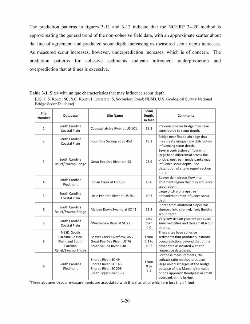
3-20
The prediction patterns in figures 3-11 and 3-12 indicate that the NCHRP 24-20 method is
approximating the general trend of the non-cohesive field data, with an approximate scatter about
the line of agreement and predicted scour depth increasing as measured scour depth increases.
As measured scour increases, however, underprediction increases, which is of concern. The
prediction patterns for cohesive sediments indicate infrequent underprediction and
overprediction that at times is excessive.
Table 3-1. Sites with unique characteristics that may influence scour depth. [US, U.S. Route; SC, S.C. Route; I, Interstate; S, Secondary Road; NBSD, U.S. Geological Survey National Bridge Scour Database]
Site Number
Database Site Name Scour Depth, in feet
Comments
1 South Carolina Coastal Plain
Coosawhatchie River at US 601 13.1 Previous smaller bridge may have contributed to scour depth.
2 South Carolina Coastal Plain
Four Hole Swamp at SC 453 13.2 Bridge near floodplain edge that may create unique flow distribution influencing scour depth.
3 South Carolina
Relief/Swamp Bridge Great Pee Dee River at I‐95 23.6
Severe contraction of flow with large head differential across the bridge; upstream guide banks may influence scour depth. See description of site in report section 3.3.1.
4 South Carolina Piedmont
Indian Creek at US 176 18.0 Beaver dam directs flow into abutment region that may influence scour depth.
5 South Carolina Coastal Plain
Little Pee Dee River at US 501 10.3 Large ditch along upstream embankment may influence scour depth.
6 South Carolina
Relief/Swamp Bridge Maiden Down Swamp at SC 41 13.8
Riprap from abutment slopes has slumped into channel, likely limiting scour depth.
7 South Carolina Coastal Plain
aWaccamaw River at SC 22 Less than 4.0
Very low stream gradient produces small velocities and thus small scour depths.
8
NBSD, South Carolina Coastal Plain, and South
Carolina Relief/Swamp Bridge
Beaver Creek Overflow, US 2 Great Pee Dee River, US 76 South Saluda River S‐40
From 0.2 to 10.2
These sites have cohesive sediments that produce substantial overprediction, beyond that of the other data associated with the respective databases.
9 South Carolina Piedmont
Enoree River, SC 49 Enoree River, SC 146 Enoree River, SC 296 South Tyger River S‐62
From 0 to 1.4
For these measurements, the setback ratio method produces large unit discharges at the bridge because of low Manning's n‐value on the approach floodplain or small overbank at the bridge.
aThree abutment‐scour measurements are associated with this site, all of which are less than 4 feet.
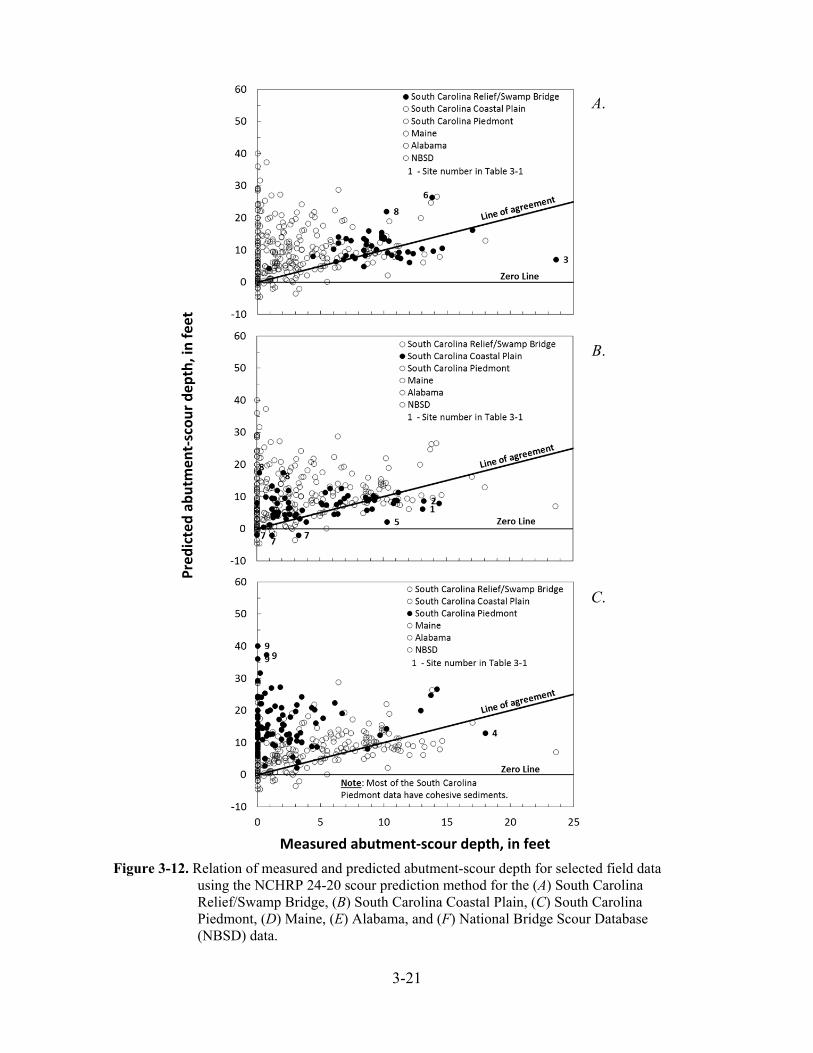
3-21
Figure 3-12. Relation of measured and predicted abutment-scour depth for selected field data using the NCHRP 24-20 scour prediction method for the (A) South Carolina Relief/Swamp Bridge, (B) South Carolina Coastal Plain, (C) South Carolina Piedmont, (D) Maine, (E) Alabama, and (F) National Bridge Scour Database (NBSD) data.
Predicted abutm
ent‐scour depth, in feet
A.
Measured abutment‐scour depth, in feet
B.
C.
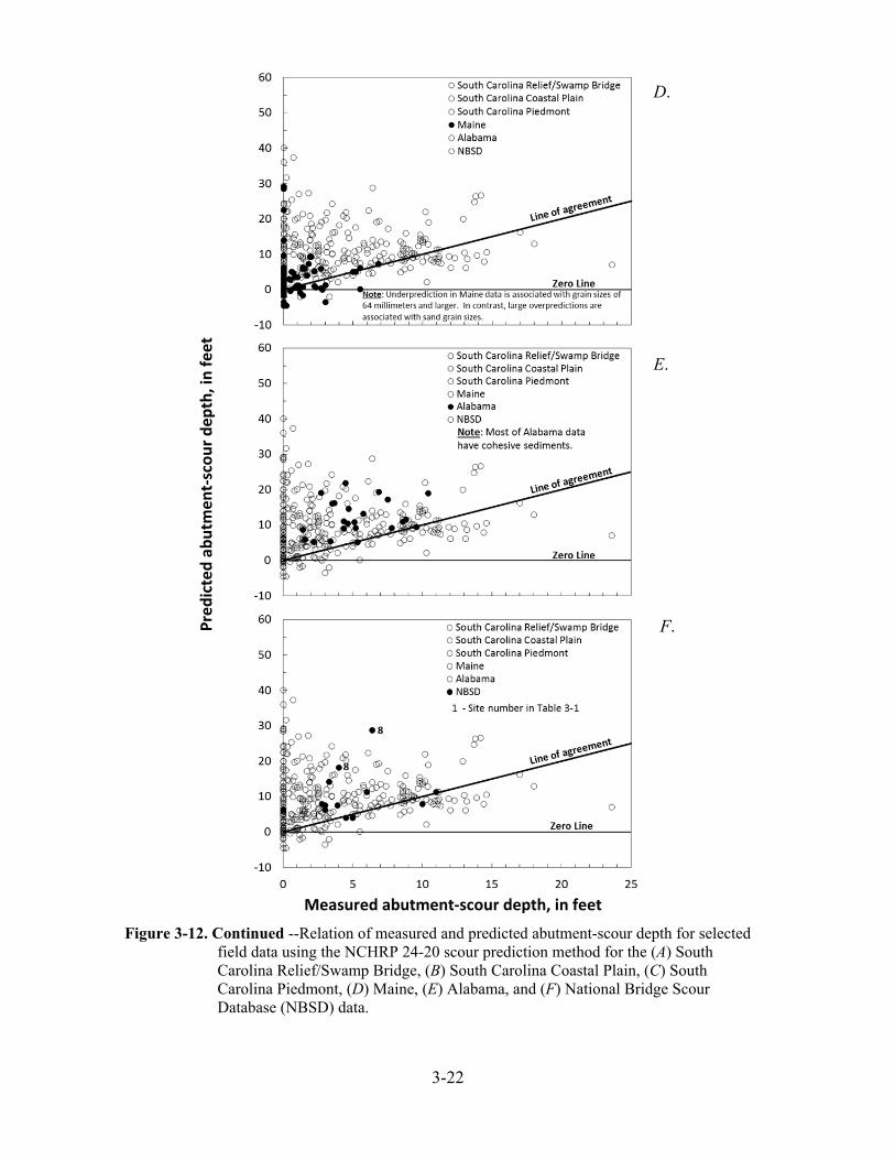
3-22
Figure 3-12. Continued --Relation of measured and predicted abutment-scour depth for selected field data using the NCHRP 24-20 scour prediction method for the (A) South Carolina Relief/Swamp Bridge, (B) South Carolina Coastal Plain, (C) South Carolina Piedmont, (D) Maine, (E) Alabama, and (F) National Bridge Scour Database (NBSD) data.
Predicted abutm
ent‐scour depth, in feet
D.
E.
F.
Measured abutment‐scour depth, in feet
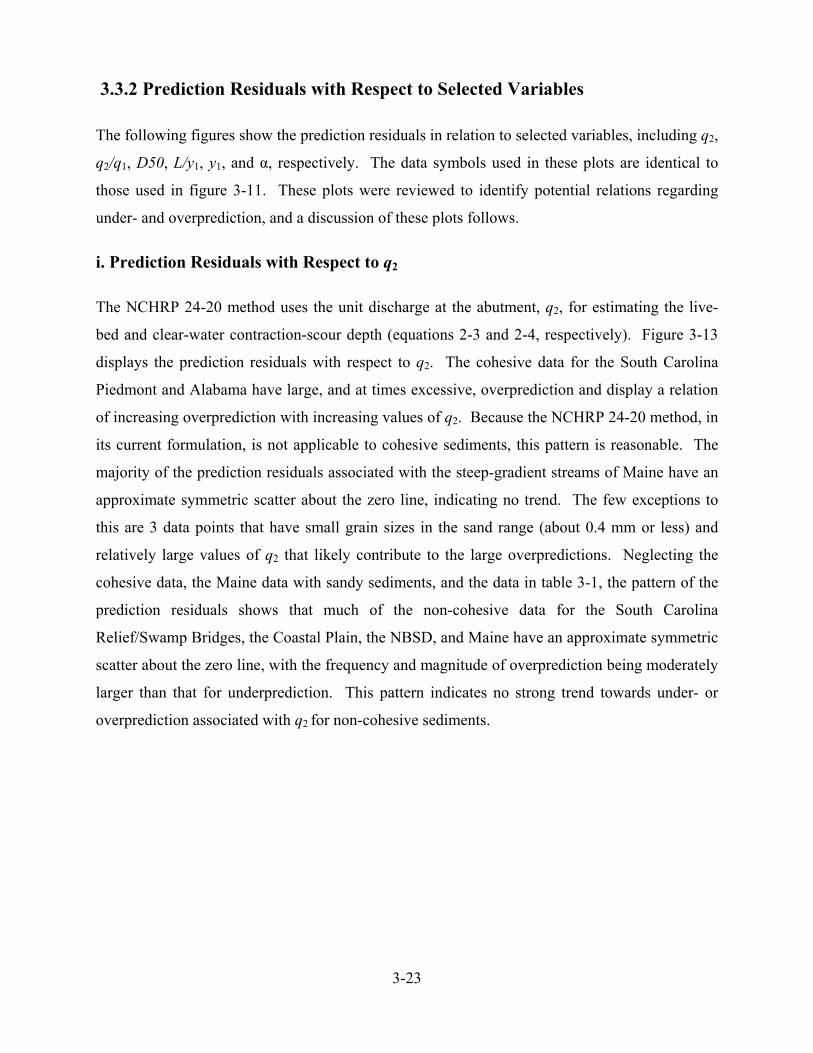
3-23
3.3.2 Prediction Residuals with Respect to Selected Variables
The following figures show the prediction residuals in relation to selected variables, including q2,
q2/q1, D50, L/y1, y1, and α, respectively. The data symbols used in these plots are identical to
those used in figure 3-11. These plots were reviewed to identify potential relations regarding
under- and overprediction, and a discussion of these plots follows.
i. Prediction Residuals with Respect to q2
The NCHRP 24-20 method uses the unit discharge at the abutment, q2, for estimating the live-
bed and clear-water contraction-scour depth (equations 2-3 and 2-4, respectively). Figure 3-13
displays the prediction residuals with respect to q2. The cohesive data for the South Carolina
Piedmont and Alabama have large, and at times excessive, overprediction and display a relation
of increasing overprediction with increasing values of q2. Because the NCHRP 24-20 method, in
its current formulation, is not applicable to cohesive sediments, this pattern is reasonable. The
majority of the prediction residuals associated with the steep-gradient streams of Maine have an
approximate symmetric scatter about the zero line, indicating no trend. The few exceptions to
this are 3 data points that have small grain sizes in the sand range (about 0.4 mm or less) and
relatively large values of q2 that likely contribute to the large overpredictions. Neglecting the
cohesive data, the Maine data with sandy sediments, and the data in table 3-1, the pattern of the
prediction residuals shows that much of the non-cohesive data for the South Carolina
Relief/Swamp Bridges, the Coastal Plain, the NBSD, and Maine have an approximate symmetric
scatter about the zero line, with the frequency and magnitude of overprediction being moderately
larger than that for underprediction. This pattern indicates no strong trend towards under- or
overprediction associated with q2 for non-cohesive sediments.
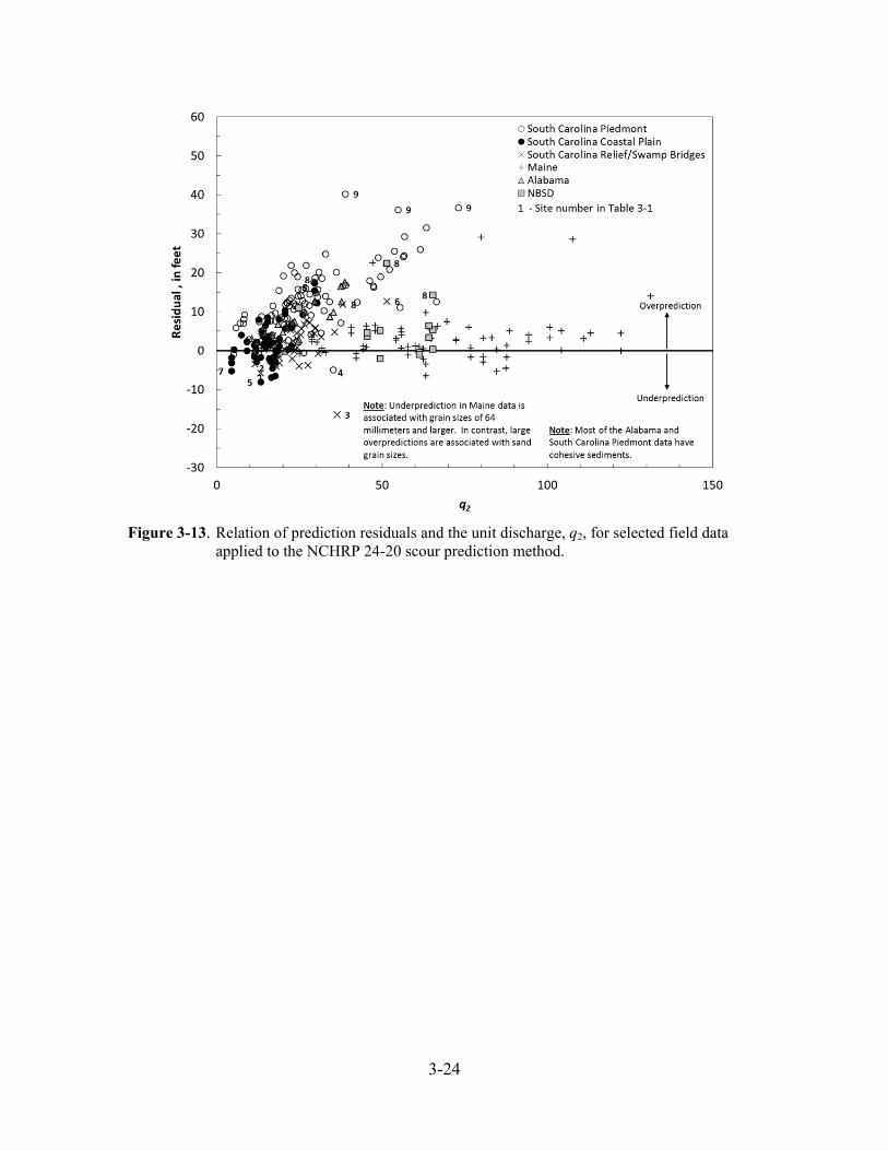
3-24
Figure 3-13. Relation of prediction residuals and the unit discharge, q2, for selected field data applied to the NCHRP 24-20 scour prediction method.
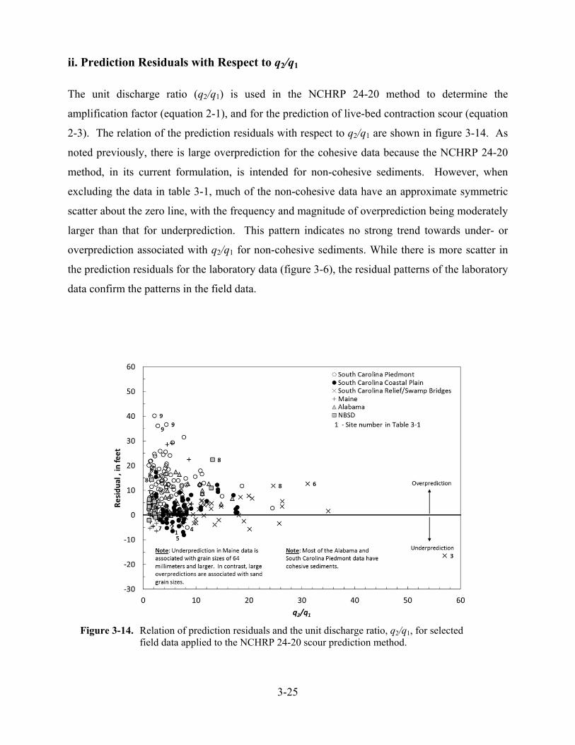
3-25
ii. Prediction Residuals with Respect to q2/q1
The unit discharge ratio (q2/q1) is used in the NCHRP 24-20 method to determine the
amplification factor (equation 2-1), and for the prediction of live-bed contraction scour (equation
2-3). The relation of the prediction residuals with respect to q2/q1 are shown in figure 3-14. As
noted previously, there is large overprediction for the cohesive data because the NCHRP 24-20
method, in its current formulation, is intended for non-cohesive sediments. However, when
excluding the data in table 3-1, much of the non-cohesive data have an approximate symmetric
scatter about the zero line, with the frequency and magnitude of overprediction being moderately
larger than that for underprediction. This pattern indicates no strong trend towards under- or
overprediction associated with q2/q1 for non-cohesive sediments. While there is more scatter in
the prediction residuals for the laboratory data (figure 3-6), the residual patterns of the laboratory
data confirm the patterns in the field data.
Figure 3-14. Relation of prediction residuals and the unit discharge ratio, q2/q1, for selected field data applied to the NCHRP 24-20 scour prediction method.
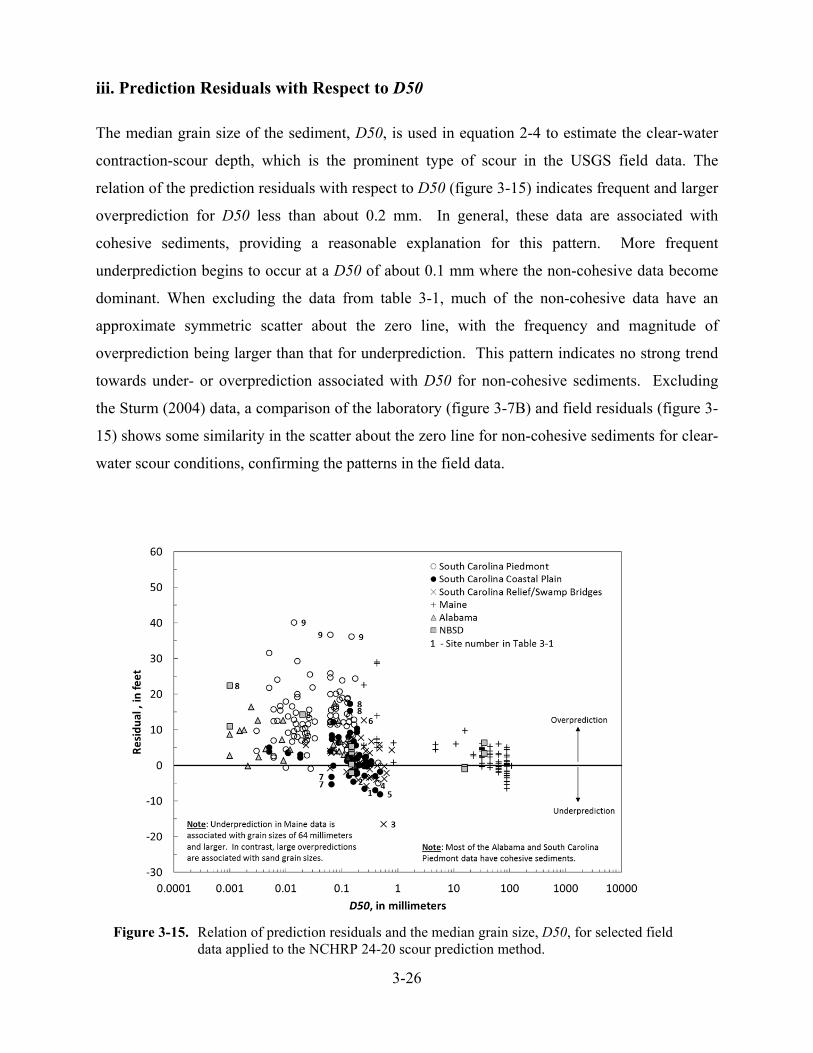
3-26
iii. Prediction Residuals with Respect to D50
The median grain size of the sediment, D50, is used in equation 2-4 to estimate the clear-water
contraction-scour depth, which is the prominent type of scour in the USGS field data. The
relation of the prediction residuals with respect to D50 (figure 3-15) indicates frequent and larger
overprediction for D50 less than about 0.2 mm. In general, these data are associated with
cohesive sediments, providing a reasonable explanation for this pattern. More frequent
underprediction begins to occur at a D50 of about 0.1 mm where the non-cohesive data become
dominant. When excluding the data from table 3-1, much of the non-cohesive data have an
approximate symmetric scatter about the zero line, with the frequency and magnitude of
overprediction being larger than that for underprediction. This pattern indicates no strong trend
towards under- or overprediction associated with D50 for non-cohesive sediments. Excluding
the Sturm (2004) data, a comparison of the laboratory (figure 3-7B) and field residuals (figure 3-
15) shows some similarity in the scatter about the zero line for non-cohesive sediments for clear-
water scour conditions, confirming the patterns in the field data.
Figure 3-15. Relation of prediction residuals and the median grain size, D50, for selected field data applied to the NCHRP 24-20 scour prediction method.
3-27
iv. Prediction Residuals with Respect to L/y1
Melville and Coleman (2000) used the relative abutment length, L/y1, to classify abutments as
short, intermediate, and long and demonstrate that the potential for abutment-scour increases as
the abutment length increases (report section 1.3.2 and figure 1-12). The relation of the
prediction residuals with respect to relative abutment length, L/y1, is shown in figure 3-16. The
figure identifies the range for short, intermediate, and long abutments as defined by Melville and
Coleman (2000) and indicates how the field data are heavily weighted towards relatively long
abutments. As noted previously, the large overprediction for the cohesive data is to be expected
from the NCHRP 24-20 method, which is intended for non-cohesive sediments in its current
formulation. When excluding the data from table 3-1, much of the non-cohesive data have an
approximate symmetric scatter about the zero line, with the frequency and magnitude of
overprediction being moderately larger than that for underprediction. This pattern indicates no
strong trend towards under- or overprediction associated with L/y1 for non-cohesive sediments.
However, if the data from table 3-1 are considered, the magnitude of underprediction increases
with increasing L/y1, indicating the potential for increased underprediction at relatively long
abutments. This is similar to the pattern in the laboratory data (figure 3-8) but not as
pronounced. While the 3 largest underpredictions (site numbers 1, 5, and 3) have unique features
that likely promote larger scour depths, it is possible that other factors, such as relatively long
abutments, contribute to this pattern. Improved estimates of the flow velocity at the abutment
from a two-dimensional flow model would likely diminish the underprediction at these sites.
However, the uncertainty in the data in figure 3-16, in conjunction with the trends of the
laboratory data (figure 3-8), indicates a need for caution and conservatism at such sites when
assessing abutment scour with the NCHRP 24-20 prediction method.
v. Prediction Residuals with Respect to y1
The approach flow depth, y1, is used directly or indirectly in equations 2-2 through 2-4 for
predicting abutment scour, and the relation of the prediction residuals with respect to y1 is shown
in figure 3-17. When excluding the data from table 3-1, much of the non-cohesive data for the
South Carolina Relief/Swamp Bridges, the Coastal Plain, the NBSD, and Maine have an
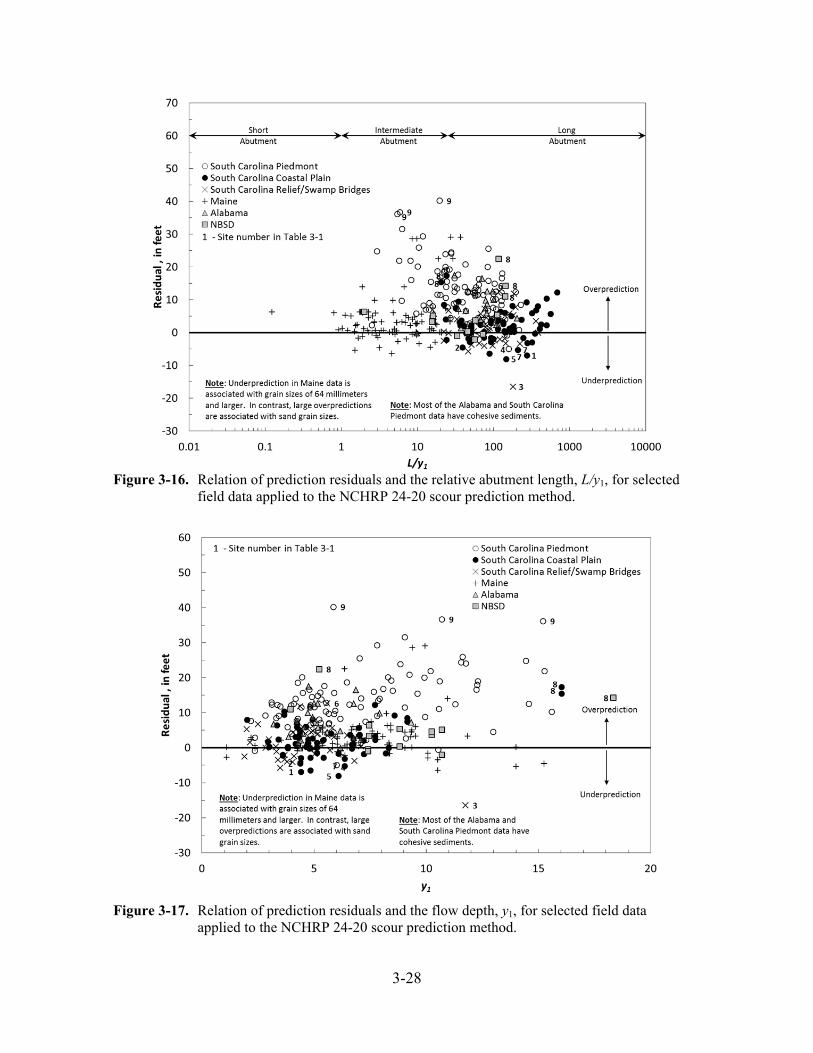
3-28
Figure 3-16. Relation of prediction residuals and the relative abutment length, L/y1, for selected field data applied to the NCHRP 24-20 scour prediction method.
Figure 3-17. Relation of prediction residuals and the flow depth, y1, for selected field data applied to the NCHRP 24-20 scour prediction method.

3-29
approximate symmetric scatter about the zero line, with the frequency and magnitude of
overprediction being moderately larger than that for underprediction. In the coarse sediments of
Maine, there is more frequent underprediction for flow depths greater than about 10 ft, indicating
a possible small trend towards underprediction with increasing flow depth. Overall, the residual
patterns for the non-cohesive sediments in the sand range indicate no strong trend towards under-
or overprediction associated with y1, while there is likely a small trend in the coarse sediments of
the Maine data. In the cohesive sediments of the South Carolina Piedmont, the magnitude of
overprediction is large and increases with increasing flow depth. The residual patterns in the
non-cohesive laboratory data (figure 3-9) differ from those of the non-cohesive field data (figure
3-17), showing an increase in overprediction with increasing flow depth, similar to the cohesive
sediments in the field data. The reason for the difference between the laboratory and field data is
unclear.
vi. Prediction Residuals with Respect to α
The amplification factor accounts for the additional scour at an abutment above and beyond the
contraction scour (equation 2-1), and the relation of the prediction residuals with respect to the
amplification factor, α, is shown in figure 3-18. The trend in the data indicates that the potential
for underprediction increases as α decreases, with the largest underprediction associated with
values of α near 1.1. This pattern is particularly evident in the long abutments associated with
South Carolina Relief/Swamp Bridge and the Coastal Plain data. If the data in table 3-1 are
excluded, the pattern is less pronounced, though still evident. While not as prominent, the longer
abutments in the laboratory data (figure 3-10) have a similar trend, with the magnitude of
underprediction increasing slightly with decreasing α. A number of field data have common
amplification factors with values of 1.1 and 1.13. These data have large values of q2/q1 that
exceed the upper bound of the amplification-factor curves (figures 2-3 through 2-6); therefore, α
was arbitrarily set to values of 1.1 or 1.13, representing the α associated with the maximum value
of q2/q1 in the curves. The South Carolina Piedmont and Alabama data have infrequent
underprediction and larger overprediction values in comparison to the other field data and is
attributed to the cohesive sediments associated with those data. A more detailed evaluation of α
is presented in the next report section.
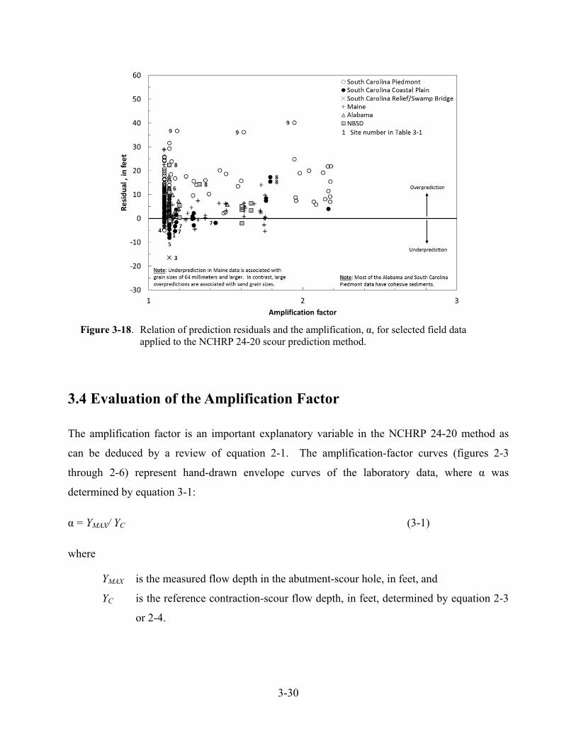
3-30
Figure 3-18. Relation of prediction residuals and the amplification, α, for selected field data applied to the NCHRP 24-20 scour prediction method.
3.4 Evaluation of the Amplification Factor
The amplification factor is an important explanatory variable in the NCHRP 24-20 method as
can be deduced by a review of equation 2-1. The amplification-factor curves (figures 2-3
through 2-6) represent hand-drawn envelope curves of the laboratory data, where α was
determined by equation 3-1:
α = YMAX/ YC (3-1)
where
YMAX is the measured flow depth in the abutment-scour hole, in feet, and
YC is the reference contraction-scour flow depth, in feet, determined by equation 2-3
or 2-4.
3-31
In a review of abutment-scour research and prediction equations, Sturm et al. (2011) made a
limited comparison of amplification factors from selected laboratory data. The relation of α and
the unit discharge ratio for wing-wall and spill-through abutments associated with the Briaud et
al. (2009) abutment-scour equation can be compared to the NCHRP 24-20 curves for Scour
Condition B (figures 2-5, 2-6, and 3-19). (Note: The Briaud et al. (2009) curves reflect design
curves with a factor of safety.) Sturm et al. (2011) notes that the peaks of the Briaud et al.
(2009) curves are higher than the NCHRP 24-20 curves and have a more gradual decrease in α as
the unit discharge increases. Sturm et al. (2011) also compares the NCHRP 24-20 α curve for
wing walls under Scour Condition B with selected data from Melville (1997), Melville and
Coleman (2000), and Sturm (2004, 2006; figure 3-20). The trends in the other laboratory data in
figure 3-20 exceed that of the NCHRP 24-20 curve. Sturm et al. (2011) attributes the difference
in the NCHRP 24-20 curves and the other laboratory data curves in figures 3-19 and 3-20 to the
differing laboratory models. The NCHRP 24-20 experiments for Scour Condition B used
erodible abutments/embankments (and not rigid abutments that extended to depth in the model
bed or floodplain) that could erode to varying degrees. Sketches of this conceptual model are
shown in figure 3-21. The erodible abutments create flow fields that tend to reduce scour depth
in comparison to rigid abutments. Data associated with erodible abutments/embankments were
used to develop the NCHRP 24-20 amplification curves for Scour Condition B, with selected
data from that investigation shown in figure 3-20. In contrast, the other laboratory data shown in
figure 3-20 represent scour associated with rigid abutment/embankment models that had rigid
substructures below the bed. These types of models tend to produce larger scour depths than the
erodible abutments in the NCHRP 24-20 experiments and provide a reasonable explanation for
the differing amplification factors in figure 3-20.
The NCHRP 24-20 study is the most extensive laboratory investigation to date of scour at
erodible abutments/embankments and provides valuable insights on abutment-scour processes at
eroded abutments and breached embankments. Additionally, Ettema et al. (2010) provide
anecdotal evidence that these types of scour processes are common occurrences in the field.
(Note: The author has seen these types of scour processes and would concur that they are
common.) While it seems appropriate to say that such scour processes are common, it would
seem incorrect to assume that they are the solitary mode of abutment scour in the field. Evidence
indicates that many abutments in the field can sustain high flows with minimal erosion and no
3-32
embankment failure. Perhaps the best example of this can be found in the USGS abutment-scour
field data where there is little indication of appreciable erosion of the abutments or embankment
breaches. As such, the USGS data represent abutment scour resulting from
abutments/embankments that remained intact during the scour process and, therefore, would
possibly have larger scour depths than those associated with eroded abutments as modeled in the
NCHRP 24-20 investigation. (Note: Vegetation growth on the embankment/abutment and
varying degrees of cohesion in the embankment fill material are a likely cause of the
embankments/abutments in the USGS data remaining intact.) This implies that the amplification
curves for the NCHRP 24-20 may be too low for intact abutments and therefore, may
underpredict scour at sites such as those in the USGS abutment-scour database. If the objective
is to design a bridge that can sustain a large flood with the abutments and embankments
remaining intact, the practitioner will need to evaluate the appropriateness of using the NCHRP
24-20 prediction method in its current formulation for the study’s design objectives. A way to
address this concern would be the inclusion of an appropriate abutment-scour countermeasure,
which is recommended as a standard design procedure by Sturm et al. (2011) for all new
abutment designs.
The trends in figures 3-19 and 3-20 indicate how amplification factors can vary substantially for
various laboratory datasets and highlight the challenge in defining this explanatory variable. It
could be argued that the amplification curves associated with the rigid-abutment models, such as
the upper curve shown in figure 3-20, is too excessive for field conditions and will produce
unrealistically large estimates of abutment scour. Some support for this argument can be found
in figure 1-21 where the upper bound of the relative scour depth for the field data (4.2) is much
smaller than that for the rigid abutment models of the Sturm (2004) data (11). However, as
previously noted, the NCHRP 24-20 amplification curves based on the erodible
abutment/embankment models may be too low for some field conditions and may produce
underprediction at abutments with minimal erosion that remain intact during a flood. To gain
insight on the range and trend of the amplification factor in the field, field data can be used to
back-calculate the required amplification factor, which is described in the following report
section.
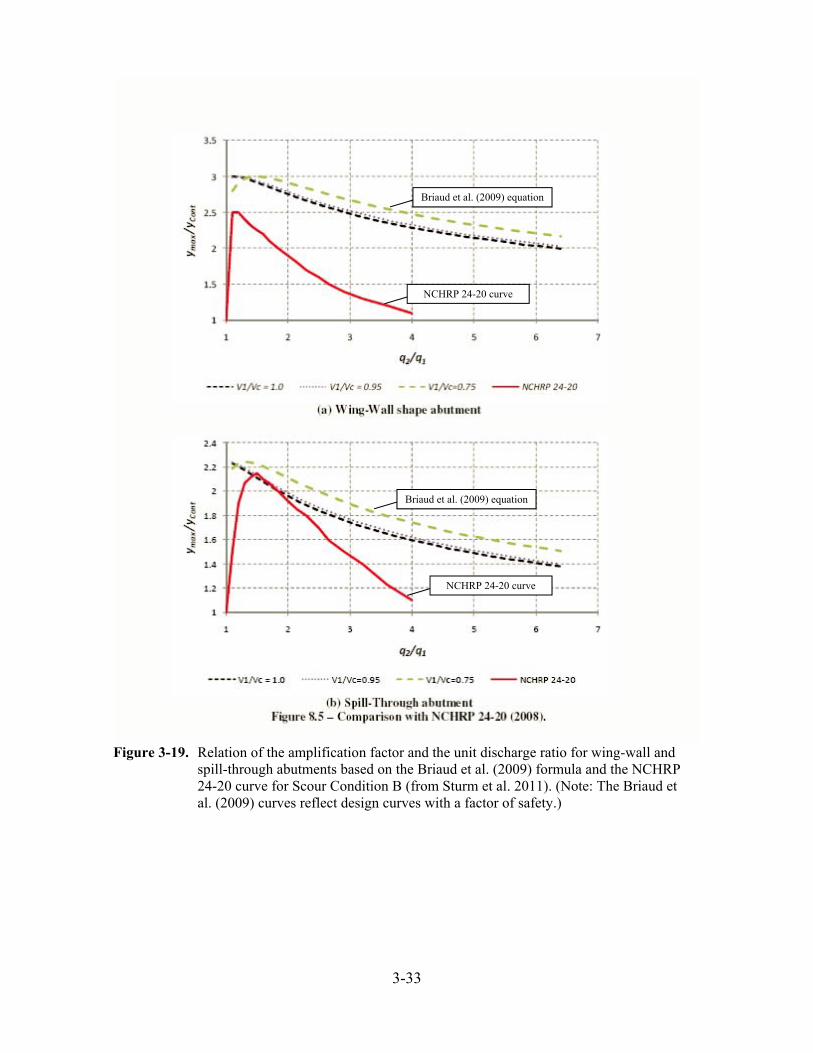
3-33
Figure 3-19. Relation of the amplification factor and the unit discharge ratio for wing-wall and spill-through abutments based on the Briaud et al. (2009) formula and the NCHRP 24-20 curve for Scour Condition B (from Sturm et al. 2011). (Note: The Briaud et al. (2009) curves reflect design curves with a factor of safety.)
NCHRP 24-20 curve
NCHRP 24-20 curve
Briaud et al. (2009) equation
Briaud et al. (2009) equation
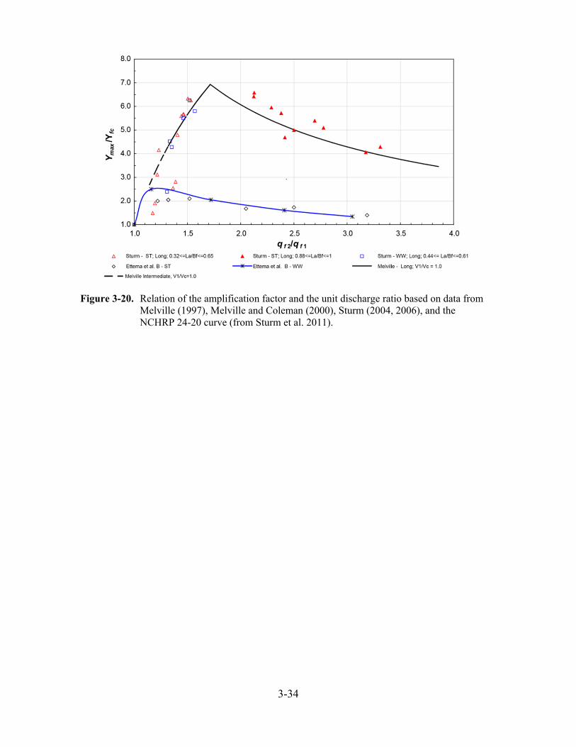
3-34
Figure 3-20. Relation of the amplification factor and the unit discharge ratio based on data from Melville (1997), Melville and Coleman (2000), Sturm (2004, 2006), and the NCHRP 24-20 curve (from Sturm et al. 2011).
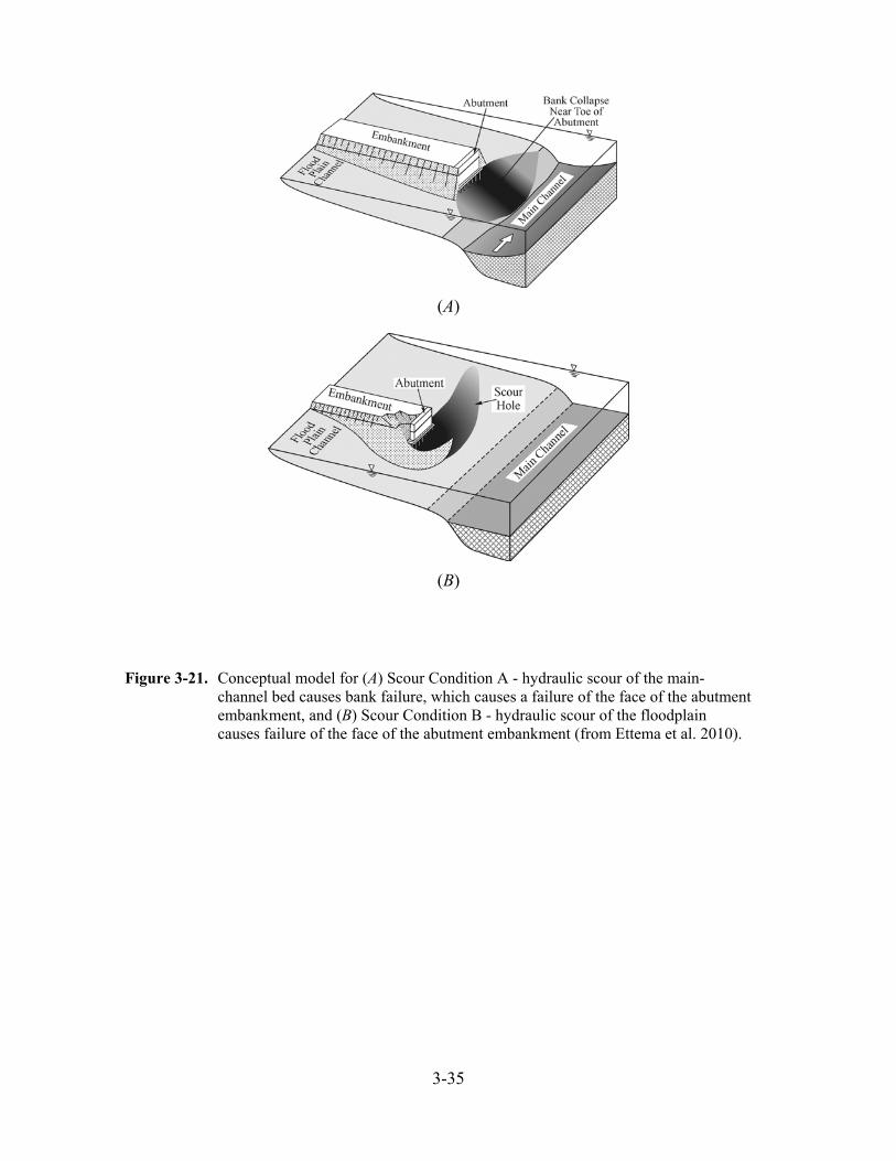
3-35
(A)
(B)
Figure 3-21. Conceptual model for (A) Scour Condition A - hydraulic scour of the main-channel bed causes bank failure, which causes a failure of the face of the abutment embankment, and (B) Scour Condition B - hydraulic scour of the floodplain causes failure of the face of the abutment embankment (from Ettema et al. 2010).
3-36
3.4.1 Determination of the Required Amplification Factor
Ettema et al. (2006) made a limited comparison of amplification factors derived from selected
field data with the NCHRP 24-20 amplification curves (figure 3-22). The selected field data in
figure 3-22 were taken from Mueller and Wagner (2005) and Benedict (2003). Ettema et al.
(2010) concluded that the limited comparison indicated that the NCHRP 24-20 amplification
curves produced scour-depth estimates that reasonably concur with those observed in the field,
but that further evaluation was needed. To gain further insights regarding the range of
amplification factors associated with field data, equation 3-1 can be used to back-calculate the
required amplification factor that would force the NCHRP 24-20 method to match the field
measurement of abutment scour. Applying equation 3-1 in this manner would require using the
field measurement to represent YMAX. The value of YC would be determined from equations 2-3
or 2-4 for the site of interest. This technique was first applied to the laboratory data (table 1-3),
and results are shown in figure 3-23. Because the NCHRP 24-20 amplification-factor curves
include only spill-through and wing-wall abutments, the laboratory data in figure 3-23 were
limited to these types of abutments. Additionally, the Sturm (2004) data associated with Scour
Condition A were excluded because of the uncertainty regarding the hydraulic conditions near
the channel. A review of figure 3-23 indicates that a substantial number of data exceed the
NCHRP 24-20 amplification-factor curves. The large amplification factors associated with the
Sturm (2004) data can be attributed, in part, to the longer relative abutment lengths associated
with those data. Neglecting the Sturm (2004) data and the 2 outliers from the Palaviccini (1993)
data, the largest required amplification factor is about 3.7. As noted by Sturm et al. (2011), the
larger amplification factors are likely created, in part, by the rigid abutments used in the other
laboratory models in contrast to the erodible abutments/embankments used in the NCHRP 24-20
models. In particular, as the scour hole develops, the rigid abutment substructure below the bed
will tend to strengthen the local flow field at the modeled abutment, thereby increasing the
potential for scour.
The required amplification factors associated with the USGS field data for Scour Conditions A
and B are shown in figure 3-24. The large scatter in this figure (3-24) is not atypical for field
data and can be attributed, in part, to the complex field conditions that diverge from those of the
laboratory, as well as the uncertainty of the field data. A large percentage of the required
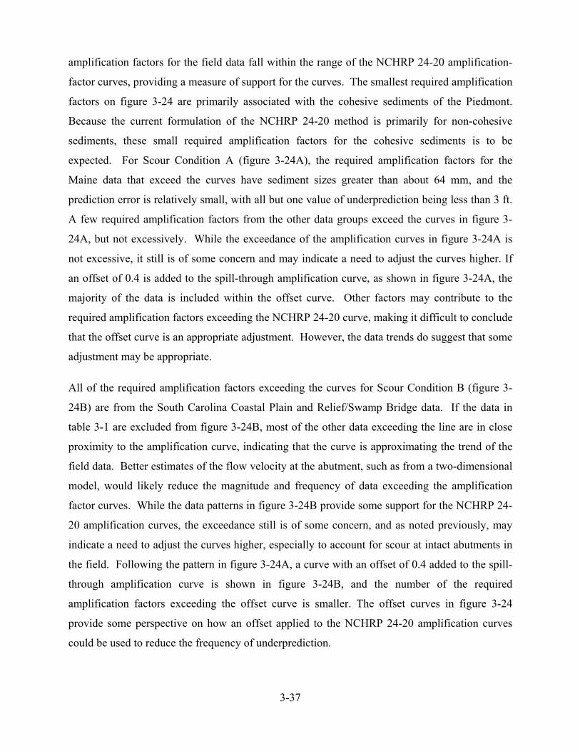
3-37
amplification factors for the field data fall within the range of the NCHRP 24-20 amplification-
factor curves, providing a measure of support for the curves. The smallest required amplification
factors on figure 3-24 are primarily associated with the cohesive sediments of the Piedmont.
Because the current formulation of the NCHRP 24-20 method is primarily for non-cohesive
sediments, these small required amplification factors for the cohesive sediments is to be
expected. For Scour Condition A (figure 3-24A), the required amplification factors for the
Maine data that exceed the curves have sediment sizes greater than about 64 mm, and the
prediction error is relatively small, with all but one value of underprediction being less than 3 ft.
A few required amplification factors from the other data groups exceed the curves in figure 3-
24A, but not excessively. While the exceedance of the amplification curves in figure 3-24A is
not excessive, it still is of some concern and may indicate a need to adjust the curves higher. If
an offset of 0.4 is added to the spill-through amplification curve, as shown in figure 3-24A, the
majority of the data is included within the offset curve. Other factors may contribute to the
required amplification factors exceeding the NCHRP 24-20 curve, making it difficult to conclude
that the offset curve is an appropriate adjustment. However, the data trends do suggest that some
adjustment may be appropriate.
All of the required amplification factors exceeding the curves for Scour Condition B (figure 3-
24B) are from the South Carolina Coastal Plain and Relief/Swamp Bridge data. If the data in
table 3-1 are excluded from figure 3-24B, most of the other data exceeding the line are in close
proximity to the amplification curve, indicating that the curve is approximating the trend of the
field data. Better estimates of the flow velocity at the abutment, such as from a two-dimensional
model, would likely reduce the magnitude and frequency of data exceeding the amplification
factor curves. While the data patterns in figure 3-24B provide some support for the NCHRP 24-
20 amplification curves, the exceedance still is of some concern, and as noted previously, may
indicate a need to adjust the curves higher, especially to account for scour at intact abutments in
the field. Following the pattern in figure 3-24A, a curve with an offset of 0.4 added to the spill-
through amplification curve is shown in figure 3-24B, and the number of the required
amplification factors exceeding the offset curve is smaller. The offset curves in figure 3-24
provide some perspective on how an offset applied to the NCHRP 24-20 amplification curves
could be used to reduce the frequency of underprediction.
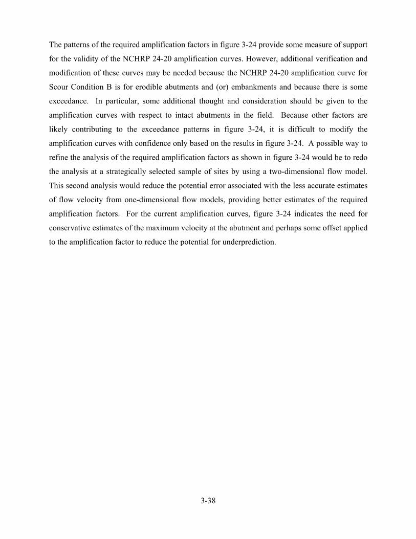
3-38
The patterns of the required amplification factors in figure 3-24 provide some measure of support
for the validity of the NCHRP 24-20 amplification curves. However, additional verification and
modification of these curves may be needed because the NCHRP 24-20 amplification curve for
Scour Condition B is for erodible abutments and (or) embankments and because there is some
exceedance. In particular, some additional thought and consideration should be given to the
amplification curves with respect to intact abutments in the field. Because other factors are
likely contributing to the exceedance patterns in figure 3-24, it is difficult to modify the
amplification curves with confidence only based on the results in figure 3-24. A possible way to
refine the analysis of the required amplification factors as shown in figure 3-24 would be to redo
the analysis at a strategically selected sample of sites by using a two-dimensional flow model.
This second analysis would reduce the potential error associated with the less accurate estimates
of flow velocity from one-dimensional flow models, providing better estimates of the required
amplification factors. For the current amplification curves, figure 3-24 indicates the need for
conservative estimates of the maximum velocity at the abutment and perhaps some offset applied
to the amplification factor to reduce the potential for underprediction.
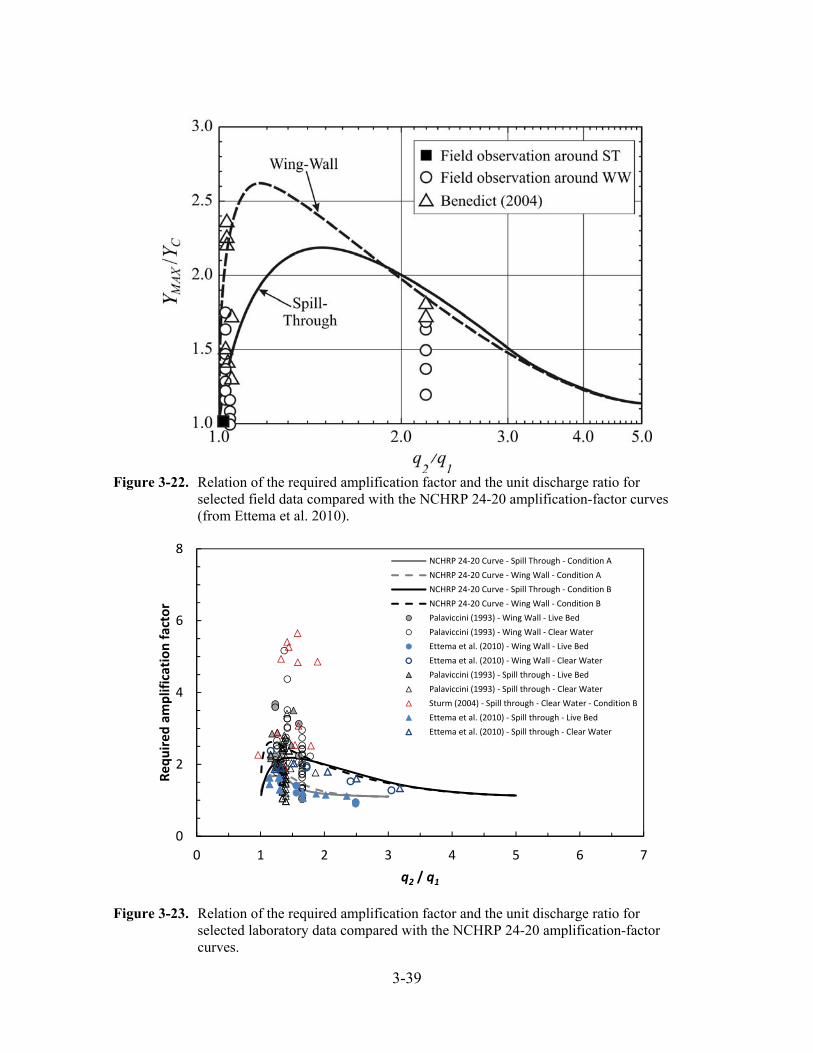
3-39
Figure 3-22. Relation of the required amplification factor and the unit discharge ratio for selected field data compared with the NCHRP 24-20 amplification-factor curves (from Ettema et al. 2010).
Figure 3-23. Relation of the required amplification factor and the unit discharge ratio for selected laboratory data compared with the NCHRP 24-20 amplification-factor curves.
0
2
4
6
8
0 1 2 3 4 5 6 7
Required amplification factor
q2 / q1
NCHRP 24‐20 Curve ‐ Spill Through ‐ Condition A
NCHRP 24‐20 Curve ‐ Wing Wall ‐ Condition A
NCHRP 24‐20 Curve ‐ Spill Through ‐ Condition B
NCHRP 24‐20 Curve ‐ Wing Wall ‐ Condition B
Palaviccini (1993) ‐ Wing Wall ‐ Live Bed
Palaviccini (1993) ‐ Wing Wall ‐ Clear Water
Ettema et al. (2010) ‐ Wing Wall ‐ Live Bed
Ettema et al. (2010) ‐ Wing Wall ‐ Clear Water
Palaviccini (1993) ‐ Spill through ‐ Live Bed
Palaviccini (1993) ‐ Spill through ‐ Clear Water
Sturm (2004) ‐ Spill through ‐ Clear Water ‐ Condition B
Ettema et al. (2010) ‐ Spill through ‐ Live Bed
Ettema et al. (2010) ‐ Spill through ‐ Clear Water
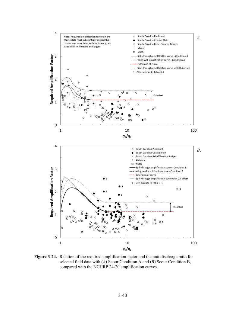
3-40
Figure 3-24. Relation of the required amplification factor and the unit discharge ratio for selected field data with (A) Scour Condition A and (B) Scour Condition B, compared with the NCHRP 24-20 amplification curves.
A.
B.
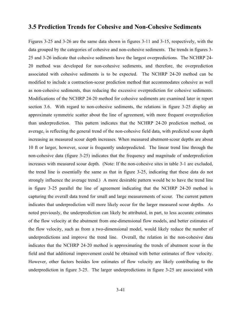
3-41
3.5 Prediction Trends for Cohesive and Non-Cohesive Sediments
Figures 3-25 and 3-26 are the same data shown in figures 3-11 and 3-15, respectively, with the
data grouped by the categories of cohesive and non-cohesive sediments. The trends in figures 3-
25 and 3-26 indicate that cohesive sediments have the largest overpredictions. The NCHRP 24-
20 method was developed for non-cohesive sediments, and therefore, the overprediction
associated with cohesive sediments is to be expected. The NCHRP 24-20 method can be
modified to include a contraction-scour prediction method that accommodates cohesive as well
as non-cohesive sediments, thus reducing the excessive overprediction for cohesive sediments.
Modifications of the NCHRP 24-20 method for cohesive sediments are examined later in report
section 3.6. With regard to non-cohesive sediments, the relations in figure 3-25 display an
approximate symmetric scatter about the line of agreement, with more frequent overprediction
than underprediction. This pattern indicates that the NCHRP 24-20 prediction method, on
average, is reflecting the general trend of the non-cohesive field data, with predicted scour depth
increasing as measured scour depth increases. When measured abutment-scour depths are about
10 ft or larger, however, scour is frequently underpredicted. The linear trend line through the
non-cohesive data (figure 3-25) indicates that the frequency and magnitude of underprediction
increases with measured scour depth. (Note: If the non-cohesive sites in table 3-1 are excluded,
the trend line is essentially the same as that in figure 3-25, indicating that these data do not
strongly influence the average trend.) A more desirable pattern would be to have the trend line
in figure 3-25 parallel the line of agreement indicating that the NCHRP 24-20 method is
capturing the overall data trend for small and large measurements of scour. The current pattern
indicates that underprediction will more likely occur for the larger measured scour depths. As
noted previously, the underprediction can likely be attributed, in part, to less accurate estimates
of the flow velocity at the abutment from one-dimensional flow models, and better estimates of
the flow velocity, such as from a two-dimensional model, would likely reduce the number of
underpredictions and improve the trend line. Overall, the relation in the non-cohesive data
indicates that the NCHRP 24-20 method is approximating the trends of abutment scour in the
field and that additional improvement could be obtained with better estimates of flow velocity.
However, other factors besides low estimates of flow velocity are likely contributing to the
underprediction in figure 3-25. The larger underpredictions in figure 3-25 are associated with
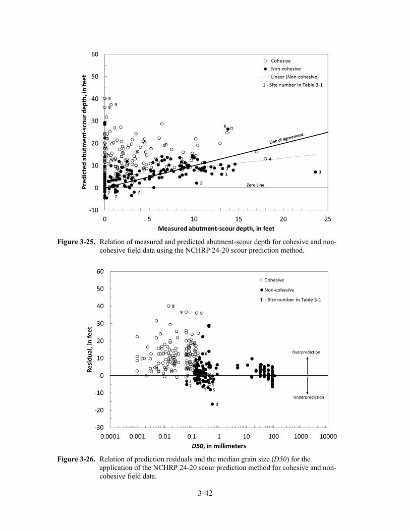
3-42
Figure 3-25. Relation of measured and predicted abutment-scour depth for cohesive and non-cohesive field data using the NCHRP 24-20 scour prediction method.
Figure 3-26. Relation of prediction residuals and the median grain size (D50) for the application of the NCHRP 24-20 scour prediction method for cohesive and non-cohesive field data.
3-43
relatively long abutments (figure 3-16) that likely have a larger potential for scour. The
laboratory data also show a pattern of larger underprediction at relatively long abutments (figure
3-8), indicating that some adjustment for longer abutments as presented in Melville and Coleman
(2000) may be a matter for consideration. While there is some uncertainty in the data in figure
3-25, the patterns indicate a need for caution and conservatism when using the NCHRP 24-20
prediction method at sites with relatively long abutments.
3.6 Alternate Critical-Velocity Methods for Estimating Clear-Water
Contraction Scour
Approximately 93 percent of the USGS field data are classified as clear-water scour and
therefore, use the clear-water contraction-scour equation (eq. 2-4) as part of the abutment-scour
computation. Equation 2-4 can be expressed in simplified form as the following:
(3-2)
where
Vc is the sediment critical velocity at which a given sediment begins to erode, in feet
per second,
and other variables are as previously defined.
The contracted unit discharge, q2, in equation 3-2 can be determined by using the SBR method as
described in chapter 2. Various methods can be used to estimate Vc. However, HEC-18
(Arneson et al. 2012) recommends using the Laursen (1963) critical-velocity equation for non-
cohesive sediments as shown in the following equation:
⁄ ⁄ (3-3)
where
y is the average flow depth, in feet;
Ku is a unit conversion factor equal to 11.17 for English units;
and Vc and D50 are as previously defined.
3-44
Substituting equation 3-3 into 3-2 leads to equation 3-4:
⁄ ⁄ (3-4)
To be physically consistent, the flow depth, y, in equation 3-4 must be equal to the flow depth in
the contraction-scour hole, YC, which yields equation 3-5:
⁄ ⁄ (3-5)
Simplifying equation 3-5 yields the same clear-water contraction-scour equation presented in
chapter 2 (equation 2-4). Equation 2-4 is a useful tool for assessing clear-water contraction-
scour flow depth. However, its application is limited to non-cohesive sediments; therefore,
HEC-18 recommends limiting the D50 to a value of 0.2 mm or greater. As can be seen in figures
3-25 and 3-26, the application of equation 2-4 to the USGS field data associated with cohesive
sediments (all of which are clear-water scour) produce substantial overprediction. This pattern
indicates that improved equation performance possibly could be achieved at sites with cohesive
sediments (median grain sizes less than 0.2 mm) by using alternate methods for estimating the
critical velocity in equation 3-2 that include critical velocities for cohesive sediments. Some
methods for consideration include Fortier and Scobey (1926), Neill (1973), and Vanoni (1975).
These alternate methods were used by Benedict (2010) in evaluating the performance of the
Maryland abutment-scour equation (Chang and Davis, 1998, 1999). A brief description of these
alternate critical-velocity methods (largely taken from Benedict, 2010) and their incorporation
into the NCHRP 24-20 method, by use of equation 3-2, follows.
3.6.1 Fortier and Scobey Maximum Permissible Velocity
In the early 1900s, focus was given to the refinement of design criteria for earthen irrigation
canals. An important component for the design criteria was the concept of the maximum
permissible velocity. A notable investigation of this phenomenon was conducted by Fortier and
Scobey (1926). This investigation was commissioned by the American Society of Civil
Engineers (ASCE) Special Committee on Irrigation Hydraulics and involved an extensive survey
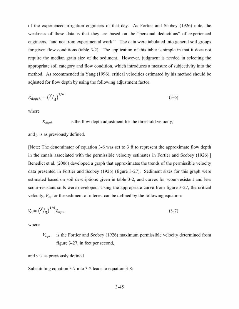
3-45
of the experienced irrigation engineers of that day. As Fortier and Scobey (1926) note, the
weakness of these data is that they are based on the “personal deductions” of experienced
engineers, “and not from experimental work.” The data were tabulated into general soil groups
for given flow conditions (table 3-2). The application of this table is simple in that it does not
require the median grain size of the sediment. However, judgment is needed in selecting the
appropriate soil category and flow condition, which introduces a measure of subjectivity into the
method. As recommended in Yang (1996), critical velocities estimated by his method should be
adjusted for flow depth by using the following adjustment factor:
3⁄
(3-6)
where
Kdepth is the flow depth adjustment for the threshold velocity,
and y is as previously defined.
[Note: The denominator of equation 3-6 was set to 3 ft to represent the approximate flow depth
in the canals associated with the permissible velocity estimates in Fortier and Scobey (1926).]
Benedict et al. (2006) developed a graph that approximates the trends of the permissible velocity
data presented in Fortier and Scobey (1926) (figure 3-27). Sediment sizes for this graph were
estimated based on soil descriptions given in table 3-2, and curves for scour-resistant and less
scour-resistant soils were developed. Using the appropriate curve from figure 3-27, the critical
velocity, Vc, for the sediment of interest can be defined by the following equation:
3⁄
(3-7)
where
Vmpv is the Fortier and Scobey (1926) maximum permissible velocity determined from
figure 3-27, in feet per second,
and y is as previously defined.
Substituting equation 3-7 into 3-2 leads to equation 3-8:
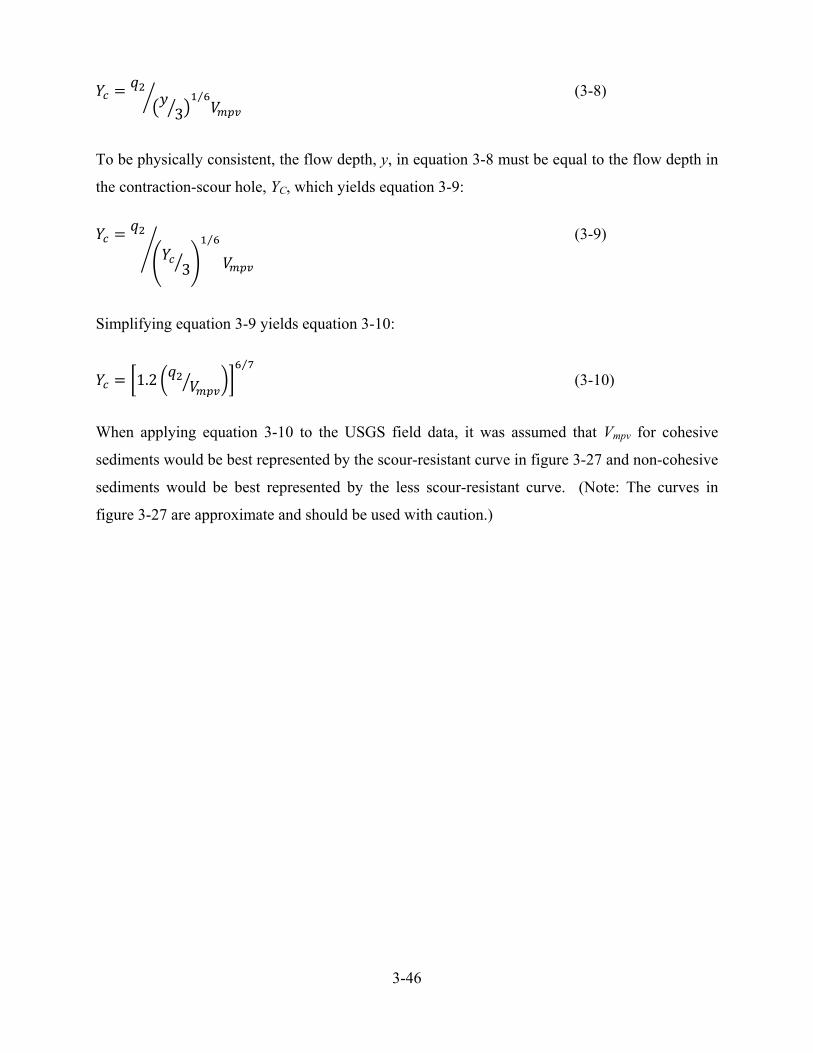
3-46
3⁄ (3-8)
To be physically consistent, the flow depth, y, in equation 3-8 must be equal to the flow depth in
the contraction-scour hole, YC, which yields equation 3-9:
3
⁄ (3-9)
Simplifying equation 3-9 yields equation 3-10:
1.2⁄
(3-10)
When applying equation 3-10 to the USGS field data, it was assumed that Vmpv for cohesive
sediments would be best represented by the scour-resistant curve in figure 3-27 and non-cohesive
sediments would be best represented by the less scour-resistant curve. (Note: The curves in
figure 3-27 are approximate and should be used with caution.)
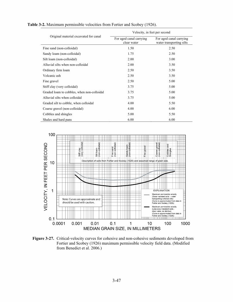
3-47
Table 3-2. Maximum permissible velocities from Fortier and Scobey (1926).
Original material excavated for canal Velocity, in feet per second
For aged canal carrying clear water
For aged canal carrying water transporting silts
Fine sand (non-colloidal) 1.50 2.50
Sandy loam (non-colloidal) 1.75 2.50
Silt loam (non-colloidal) 2.00 3.00
Alluvial silts when non-colloidal 2.00 3.50
Ordinary firm loam 2.50 3.50
Volcanic ash 2.50 3.50
Fine gravel 2.50 5.00
Stiff clay (very colloidal) 3.75 5.00
Graded loam to cobbles, when non-colloidal 3.75 5.00
Alluvial silts when colloidal 3.75 5.00
Graded silt to cobble, when colloidal 4.00 5.50
Coarse gravel (non-colloidal) 4.00 6.00
Cobbles and shingles 5.00 5.50
Shales and hard pans 6.00 6.00
Figure 3-27. Critical-velocity curves for cohesive and non-cohesive sediments developed from
Fortier and Scobey (1926) maximum permissible velocity field data. (Modified from Benedict et al. 2006.)
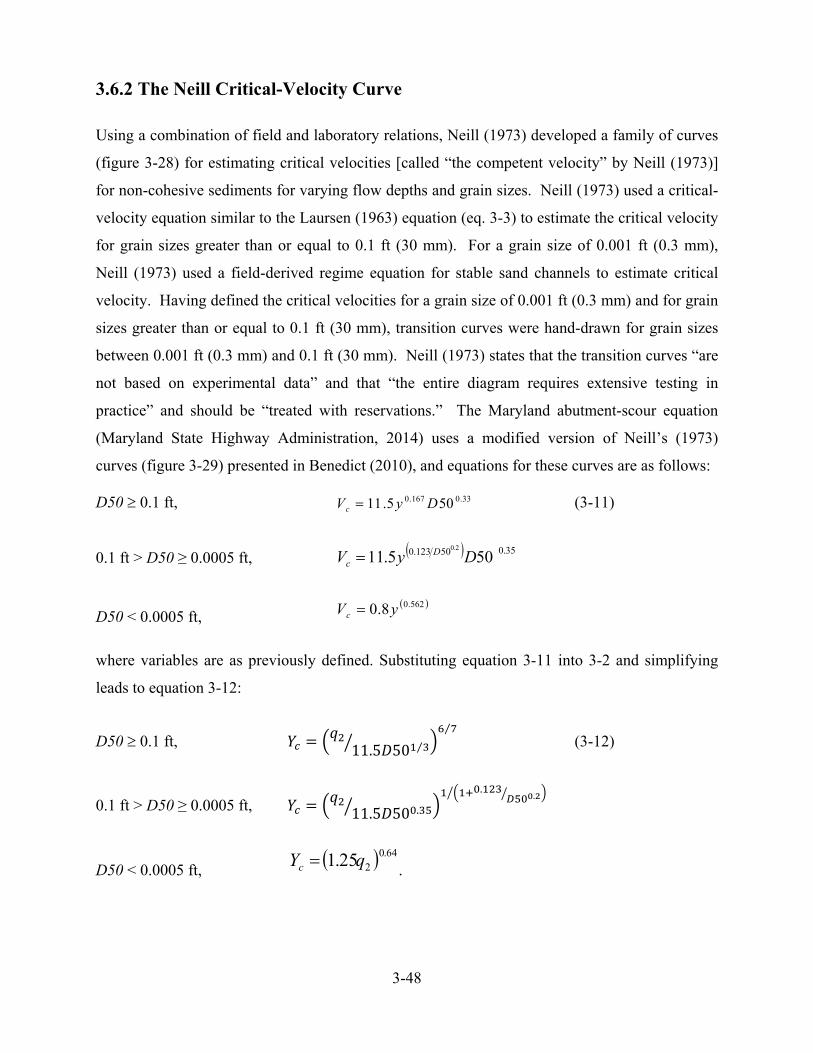
3-48
3.6.2 The Neill Critical-Velocity Curve
Using a combination of field and laboratory relations, Neill (1973) developed a family of curves
(figure 3-28) for estimating critical velocities [called “the competent velocity” by Neill (1973)]
for non-cohesive sediments for varying flow depths and grain sizes. Neill (1973) used a critical-
velocity equation similar to the Laursen (1963) equation (eq. 3-3) to estimate the critical velocity
for grain sizes greater than or equal to 0.1 ft (30 mm). For a grain size of 0.001 ft (0.3 mm),
Neill (1973) used a field-derived regime equation for stable sand channels to estimate critical
velocity. Having defined the critical velocities for a grain size of 0.001 ft (0.3 mm) and for grain
sizes greater than or equal to 0.1 ft (30 mm), transition curves were hand-drawn for grain sizes
between 0.001 ft (0.3 mm) and 0.1 ft (30 mm). Neill (1973) states that the transition curves “are
not based on experimental data” and that “the entire diagram requires extensive testing in
practice” and should be “treated with reservations.” The Maryland abutment-scour equation
(Maryland State Highway Administration, 2014) uses a modified version of Neill’s (1973)
curves (figure 3-29) presented in Benedict (2010), and equations for these curves are as follows:
D50 0.1 ft, 33.0167.0 505.11 DyVc (3-11)
0.1 ft > D50 ≥ 0.0005 ft, 35.050123.0 505.112.0
DyV Dc
D50 < 0.0005 ft, 562.08.0 yVc
where variables are as previously defined. Substituting equation 3-11 into 3-2 and simplifying
leads to equation 3-12:
D50 0.1 ft, 11.5 50 ⁄
⁄ (3-12)
0.1 ft > D50 ≥ 0.0005 ft, 11.5 50 .
..
D50 < 0.0005 ft, 64.0
225.1 qYc .
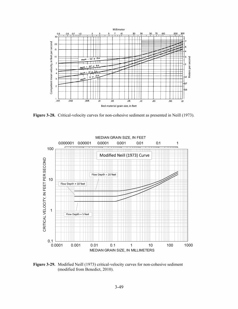
3-49
Figure 3-28. Critical-velocity curves for non-cohesive sediment as presented in Neill (1973).
Figure 3-29. Modified Neill (1973) critical-velocity curves for non-cohesive sediment (modified from Benedict, 2010).
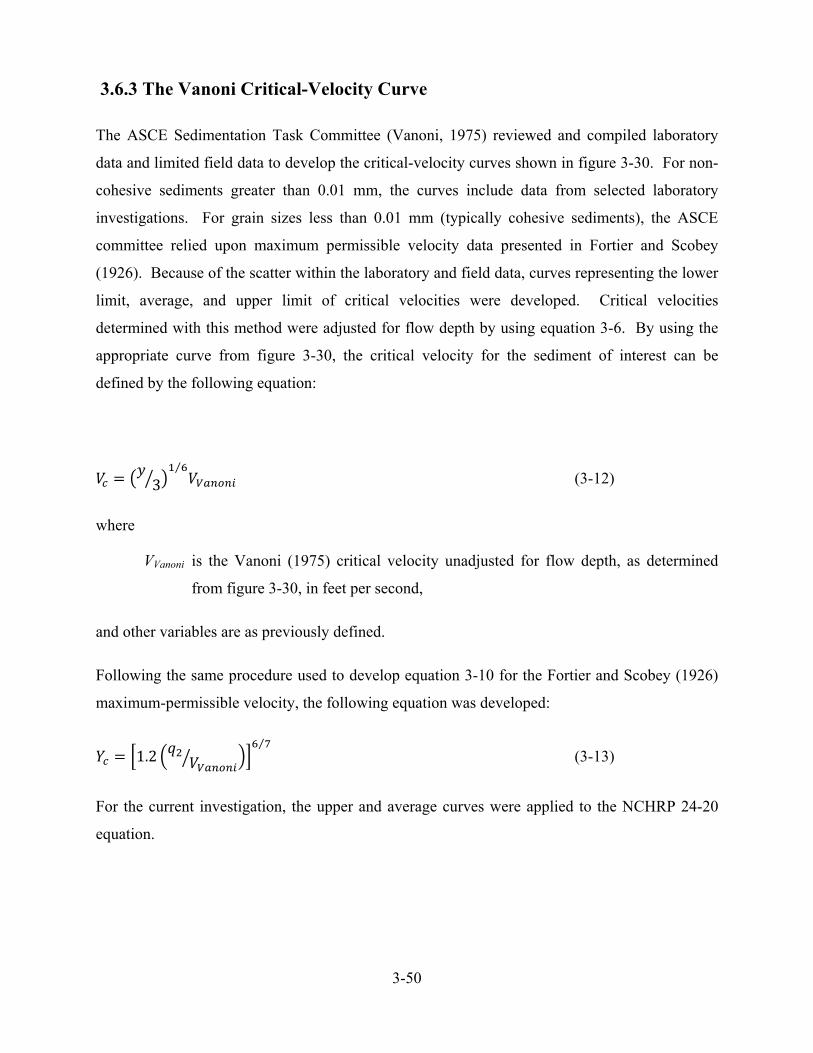
3-50
3.6.3 The Vanoni Critical-Velocity Curve
The ASCE Sedimentation Task Committee (Vanoni, 1975) reviewed and compiled laboratory
data and limited field data to develop the critical-velocity curves shown in figure 3-30. For non-
cohesive sediments greater than 0.01 mm, the curves include data from selected laboratory
investigations. For grain sizes less than 0.01 mm (typically cohesive sediments), the ASCE
committee relied upon maximum permissible velocity data presented in Fortier and Scobey
(1926). Because of the scatter within the laboratory and field data, curves representing the lower
limit, average, and upper limit of critical velocities were developed. Critical velocities
determined with this method were adjusted for flow depth by using equation 3-6. By using the
appropriate curve from figure 3-30, the critical velocity for the sediment of interest can be
defined by the following equation:
3⁄
(3-12)
where
VVanoni is the Vanoni (1975) critical velocity unadjusted for flow depth, as determined
from figure 3-30, in feet per second,
and other variables are as previously defined.
Following the same procedure used to develop equation 3-10 for the Fortier and Scobey (1926)
maximum-permissible velocity, the following equation was developed:
1.2⁄
(3-13)
For the current investigation, the upper and average curves were applied to the NCHRP 24-20
equation.
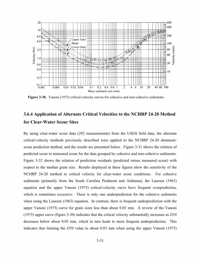
3-51
Figure 3-30. Vanoni (1975) critical-velocity curves for cohesive and non-cohesive sediments.
3.6.4 Application of Alternate Critical Velocities to the NCHRP 24-20 Method
for Clear-Water Scour Sites
By using clear-water scour data (292 measurements) from the USGS field data, the alternate
critical-velocity methods previously described were applied to the NCHRP 24-20 abutment-
scour prediction method, and the results are presented below. Figure 3-31 shows the relation of
predicted scour to measured scour for the data grouped by cohesive and non-cohesive sediments.
Figure 3-32 shows the relation of prediction residuals (predicted minus measured scour) with
respect to the median grain size. Results displayed in these figures show the sensitivity of the
NCHRP 24-20 method to critical velocity for clear-water scour conditions. For cohesive
sediments (primarily from the South Carolina Piedmont and Alabama), the Laursen (1963)
equation and the upper Vanoni (1975) critical-velocity curve have frequent overprediction,
which is sometimes excessive. There is only one underprediction for the cohesive sediments
when using the Laursen (1963) equation. In contrast, there is frequent underprediction with the
upper Vanoni (1975) curve for grain sizes less than about 0.03 mm. A review of the Vanoni
(1975) upper curve (figure 3-30) indicates that the critical velocity substantially increases as D50
decreases below about 0.03 mm, which in turn leads to more frequent underprediction. This
indicates that limiting the D50 value to about 0.03 mm when using the upper Vanoni (1975)
3-52
curve for cohesive sediments may yield better results for sites with a D50 less than 0.03 mm.
The Fortier and Scobey (1926) and modified Neill (1973) methods have similar prediction
patterns for the cohesive data, with prediction residuals following more closely to the line of
agreement (figure 3-31). The overpredictions are not as excessive as those for the Laursen
(1963) and Vanoni (1975) methods. However, the underprediction for the Fortier and Scobey
(1926) and modified Neill (1973) methods is of some concern.
With regard to the non-cohesive sediments, the Laursen (1963) and Fortier and Scobey (1926)
methods have similar patterns with an approximate symmetry about the line of agreement (figure
3-31), with the Laursen (1963) method following the line of agreement more closely. However,
underprediction tends to increase in magnitude as measured scour increases for both methods.
The modified Neill (1973) method has the largest number of underpredictions for the non-
cohesive sediments. The upper Vanoni (1975) curve has the smallest number of underpredictions
for the non-cohesive sediments, and the underprediction for the largest observed scour (23.6 ft) is
smaller than for the other critical-velocity methods.
The underprediction in figure 3-31 likely is caused, in part, by the less accurate estimates of flow
velocity from the one-dimensional flow models, and performance could vary with better
estimates of flow velocity. This should be kept in mind when evaluating the results. The
patterns in figure 3-32 indicate that the Laursen (1963) method, currently used in the NCHRP
24-20 prediction method, is a reasonable method for non-cohesive sediments and
underprediction possibly may be minimized with better estimates of flow velocity. For a more
conservative estimate of abutment scour in non-cohesive sediments, the upper Vanoni (1975)
curve may be appropriate. For cohesive sediments, the Fortier and Scobey (1926) and modified
Neill (1973) methods minimize the excessive overprediction associated with the Laursen (1963)
method. However, the frequent underprediction with these methods is of concern.
Benedict (2010) conducted a similar analysis with the Maryland abutment-scour equation
(Chang and Davis, 1998, 1999) only using the South Carolina field data, and the results are
shown in figure 3-33. The Maryland abutment-scour equation is similar in form to that of the
NCHRP 24-20 method, with abutment scour being a function of contraction scour amplified by a
series of amplification coefficients. A comparison of figures 3-31 and 3-33 shows similar
prediction patterns between the two methods, highlighting the similarity of equation
3-53
performance. (Note: The different scales in figures 3-31 and 3-33 should be kept in mind when
making comparisons.) The data applied to the Maryland equation in figure 3-33 are the South
Carolina data grouped by the Piedmont and Coastal Plain regions. With only a few exceptions,
these data correspond to cohesive and non-cohesive sediments, respectively, allowing a
reasonable comparison to the cohesive and non-cohesive data in figure 3-31. Some application
differences between the Maryland equation (figure 3-33) and the NCHRP 24-20 equation (figure
3-31) are as follows, and these should be kept in mind when making comparisons between the
methods.
The Maryland equation sets all negative scour prediction values to zero. In contrast,
the application of the NCHRP 24-20 equation in figure 3-31 retains all negative
values.
The computation of the critical velocity in the Maryland equation (figure 3-31) used
the actual D50 and did not limit the D50 to 0.2 mm. In contrast, the NCHRP 24-20
method (figure 3-31) set the D50 to 0.2 mm if the actual D50 was less than 0.2 mm.
Therefore, sites having a D50 less than 0.2 mm will tend to produce larger abutment-
scour depths with the Maryland equation than with the NCHRP 24-20 method. A
review of table 1-1 indicates that many of the USGS field data have D50s less than
0.2 mm, which will tend to produce more overprediction in the Maryland equation in
contrast to the NCHRP 24-20 method. This trend is particularly noticeable in the
cohesive sediments where D50s generally are less than 0.2 mm. The limiting of the
D50s to a value of 0.2 mm in the NCHRP 24-20 method is likely a primary reason
why that method produces less overprediction than the Maryland equation.
A comparison of non-cohesive sediments in figure 3-31 with the Coastal Plain data
(also non-cohesive) in figure 3-33 indicates that the Maryland and NCHRP 24-20
methods have similar patterns of prediction. However, the NCHRP 24-20 prediction
method generally has smaller overpredictions and smaller scatter about the line of
agreement. Table 1-1 indicates that many of the non-cohesive data have D50s less
than 0.2 mm and, as described previously, this is likely a primary reason for the
differing prediction patterns between the Maryland equation and the NCHRP 24-20
method.

3-54
Based on the analysis of the Maryland equation by Benedict (2010; figure 3-33), the
Maryland State Highway Administration (2014) recommends using the modified
Neill (1973) critical-velocity curves (figure 3-29) in the Maryland equation for sites
having characteristics similar to the Piedmont Physiographic Province of South
Carolina. The Vanoni (1975) critical-velocity curves (figure 3-30) are recommended
for sites having characteristics similar to the Coastal Plain Physiographic Province of
South Carolina. Additionally, the Maryland State Highway Administration (2014)
recommends safety factors be applied to the Maryland equation.
Figure 3-31. Relation of measured and predicted abutment-scour depth for the NCHRP 24-20
scour prediction method using field data and selected critical-velocity methods. (Numbers in graphs refer to sites in table 3-1.)
Pre
dict
ed s
cour
, in
feet
Measured scour, in feet
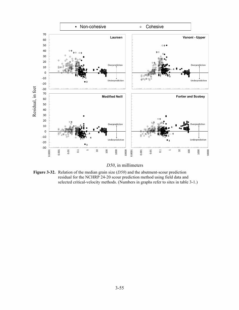
3-55
Figure 3-32. Relation of the median grain size (D50) and the abutment-scour prediction residual for the NCHRP 24-20 scour prediction method using field data and selected critical-velocity methods. (Numbers in graphs refer to sites in table 3-1.)
Res
idua
l, in
fee
t
D50, in millimeters

3-56
Figure 3-33. Relation of measured and predicted abutment-scour depth for Maryland abutment-
scour equation (Chang and Davis, 1998, 1999) using field data and selected critical-velocity methods (from Benedict, 2010).
3-57
3.7 Assessment of the NCHRP 24-20 Prediction Method
Based on the review of the NCHRP 24-20 prediction method (Ettema et al. 2010; Arneson et al.
2012) and the analysis associated with the laboratory and USGS field data, a limited assessment
of the method will be presented, including noted strengths and weaknesses, recommended
analyses for further verification of the method’s performance, and limited guidance for applying
the method. The complexity of scour processes at abutments and the limitations of the data used
in this analysis make it difficult to fully evaluate the performance of the NCHRP 24-20
prediction method. The following report sections should be viewed in light of this challenge.
3.7.1 Strengths
The strengths of the NCHRP 24-20 abutment-scour prediction method include the following:
1. Simple conceptual model based on physical processes:
The method uses a simple conceptual model based on accepted physical processes
associated with hydraulics and sediment transport, in which abutment scour is considered
a function of contraction scour. The conceptual model provides a logical explanation of
the relation between abutment and contraction scour helping clarify the long-standing
question regarding the additive nature (or lack thereof) of these scour components.
Additionally, its derivation from physical processes should allow the equation to have
broad application to a variety of field conditions.
2. Uses well-accepted and familiar equations:
The current formulation of the NCHRP 24-20 method uses the live-bed and clear-water
contraction-scour equations developed by Laursen (1960; 1963). These equations are
well accepted, have broad application, and should be familiar to the practitioner.
3. Method potentially can be extended to include cohesive sediments:
The current formulation of the NCHRP 24-20 method is for non-cohesive sediments.
However, the conceptual model is applicable to cohesive sediments, and with an
3-58
appropriate contraction-scour equation, the method could be adapted for the prediction of
abutment scour in cohesive sediments.
4. Has some underprediction, but tends to capture trend of non-cohesive data:
While there is some underprediction in the application of the non-cohesive field data to
the NCHRP 24-20 method, the prediction patterns in figure 3-25 indicate that the method
is reflecting the general trend of the non-cohesive field data, with predicted scour depth
increasing as measured scour depth increases, particularly for measured scour depths less
than about 10 ft. The underprediction is of concern, but could likely be reduced, in some
measure, with better estimates of flow velocity at the abutment using a two-dimensional
flow model.
3.7.2 Weaknesses
The weaknesses of the NCHRP 24-20 abutment-scour prediction method include the following:
1. Erodible abutments/embankments for Scour Condition B yield smaller scour depths
than intact abutments:
The conceptual model for Scour Condition B (relatively large abutment setbacks)
assumes erodible abutments/embankments that can erode (figure 3-21). These conditions
produce smaller abutment-scour depths than those of rigid abutment models (figure 3-
20), which treat abutments as solid bodies extending to depth in a channel bed or
floodplain. While scour processes associated with Scour Condition B are common in the
field, it would be incorrect to assume that they are the only mode of abutment scour.
Rather, these scour processes should be viewed as one of multiple modes. Many
abutments remain intact during high flows, with minimal erosion and no embankment
failure. For intact abutments in the field under Scour Condition B, the NCHRP 24-20
prediction method may underpredict scour. While multiple factors likely contribute to
the underprediction in figure 3-25, the erodible abutment/embankment data for Scour
Condition B in NCHRP 24-20 likely play some role. Because of the differing scour
patterns between erodible and intact abutments, the practitioner will need to evaluate the
appropriateness of using the NCHRP 24-20 prediction method for abutments with Scour
3-59
Condition B. (See report section 3.4 for additional details.) A way to address this
concern would be the inclusion of an appropriate abutment-scour countermeasure, which
is recommended as a standard design procedure by Sturm et al. (2011) for all new
abutment designs.
2. Laboratory data do not include the range of embankment lengths and flow
contractions measured in the field where potential for scour is greatest:
The challenges of the laboratory make it difficult to develop models that reflect the full
range of abutment lengths and flow contractions measured in the field. Therefore, the
ranges of L/y1 (figure 1-13) and q2/q1 (figure 1-15) for the field data are larger than that of
the laboratory data, indicating that the field data represent more severe contractions of
flow, where scour potential is greatest, than those represented by the laboratory data.
Long abutments and large contractions can create large head differentials across a bridge,
creating adverse conditions for scour. Because the NCHRP 24-20 laboratory data do not
encompass the range of the field data, scour may be underpredicted at such sites. It is
notable that the most severe flow contraction (q2/q1 equals about 50) in the USGS
abutment-scour database (Pee Dee River at I-95) has the largest measured scour depth
(23.6 ft), but also has the largest underprediction (figure 3-11) with the NCHRP 24-20
method. While other factors likely contribute to this underprediction, the severe flow
contraction that greatly exceeds the range of the laboratory data likely plays some role.
(For additional details, see the discussions about figures 1-15 and 1-24 in report sections
1.4.1 and 1.4.4, respectively.)
3. Large overprediction for cohesive sediments:
Figure 3-25 shows the prediction patterns for cohesive and non-cohesive sediments and
indicates infrequent underprediction for cohesive sediments and overprediction that at
times is excessive. The current formulation for the NCHRP 24-20 method is for non-
cohesive sediments; therefore, the method is expected to overpredict for cohesive
sediments.
3-60
4. Increasing underprediction with increasing measured scour for non-cohesive
sediments:
While the prediction patterns for non-cohesive sediments in figure 3-25 are capturing the
general trend of the field data for measured scour depths less than 10 ft, there is a trend of
increasing underprediction as measured scour increases beyond 10 ft. The laboratory
data show a similar trend, although not as severe, with increased underprediction as
measured scour increases (figures 3-2 through 3-4). This pattern is of concern and
indicates that abutment scour at sites having the largest potential for scour will tend to be
underpredicted. The exact cause of this underprediction is difficult to determine and, as
noted previously, is likely caused by multiple factors. Better estimates of flow velocity at
the abutment from a two-dimensional model would likely improve results. This
underprediction is most notable in the low-gradient streams of the South Carolina Coastal
Plain data that generally have wide densely-vegetated floodplains, severe contractions of
flow, and some of the largest measured scour depths. This pattern of underprediction
indicates a need for caution when assessing scour at such sites.
5. Differing sediment characteristics between laboratory and field:
Laboratory experiments typically use uniform non-cohesive sediments. In contrast,
sediments in the field are non-uniform in grain size and often have varying degrees of
cohesion. Additionally, natural streams typically have scour-resistant subsurface strata
that impede or limit scour depths (see report section 1.2.5). These characteristics tend to
reduce scour depths in the field below those associated with laboratory investigations
(figure 1-21). The erodible abutments/embankments for the NCHRP 24-20 data (Scour
Condition B) also tend to produce smaller scour depths than those associated with rigid
abutment models (figure 1-12). It is interesting to note that the upper bounds of the field
data and the NCHRP 24-20 data are approximately the same (figure 1-21). While the
USGS field data and the NCHRP 24-20 laboratory data both have reduced scour depths
in comparison to rigid abutment models, the mechanisms that produced the smaller scour
depths may differ (see report section 1.2.5). If a field site has conditions where the depth
of the erodible sediments was very large, allowing scour depths to exceed those of the
USGS field data, the NCHRP 24-20 method may tend to have larger underprediction.
3-61
3.7.3 Recommendations for Additional Analysis
The analysis presented in this report indicates that the NCHRP 24-20 method is capturing the
general trends of scour in the field for non-cohesive sediments, but still has some
underprediction that is of concern. The following recommendations are made with the goal of
identifying the cause of underprediction and minimizing it. Other factors likely contribute to
underprediction, but they are not addressed here.
1. Evaluating sensitivity to flow velocity:
The prediction patterns in the non-cohesive sediments of the USGS field data (figure 3-
25) indicate that the NCHRP 24-20 method is reflecting the general trend of the field
data, but with increasing magnitude and frequency of underprediction as measured scour
increases. The uncertainty of the USGS field data makes it difficult to determine the
exact cause of the underprediction pattern. Better estimates of flow velocity near the
abutment may improve performance. This assumption could be evaluated by selecting a
strategic sample of sites from the USGS field database, developing two-dimensional flow
models for the sites, and applying the better estimates of flow velocity to the NCHRP 24-
20 method. This analysis would help identify how sensitive the NCHRP 24-20 method is
to the estimate of flow velocity at the abutment. If prediction is substantially improved,
this would indicate that prediction error from other factors may be negligible, providing a
direction for further improving performance.
2. Evaluating the Scour Condition B amplification factor for field conditions where the
abutment/embankment remain intact:
The current amplification curves for Scour Condition B represent abutment scour
associated with eroded abutments/embankments that produce smaller abutment-scour
depths than rigid abutments (see report section 3.4). While it can be argued that the rigid
abutment models typically used in laboratory investigations will tend to produce larger
relative scour depths than those found in the field, the erodible abutment/embankments
models used in the NCHRP 24-20 investigation may produce smaller scour depths than
those associated with abutments in the field that remain intact during a flood. The

3-62
required amplification factors shown in figure 3-24 indicate that there may be some
justification in modifying the amplification curves. Using the results from the evaluation
of the sensitivity of the NCHRP 24-20 method to flow velocity (see item 1 above), the
required amplification factor could be reanalyzed (see report section 3.4.1) to gain
insights about this factor. Also, consideration should be given on how to model intact
abutments in the laboratory that better reflect field conditions that could be used to
evaluate the amplification factor for intact abutments.
3. Long abutments:
Melville (1992) and Melville and Coleman (2000) note that the reduction in scour depth
derived from streamlined abutment shapes, such as the spill-through and wing-wall
abutments, diminishes as abutment length increases, and for longer abutments, scour
depths approach those for a vertical wall regardless of abutment shape. This pattern was
observed in laboratory data associated with rigid abutment models and will likely differ
or be absent from scour patterns for erodible abutments/embankments such as those used
in the NCHRP 24-20 investigation for Scour Condition B. Therefore, the exclusion of an
adjustment factor for relatively long abutments from the NCHRP 24-20 method is
reasonable. In the field setting, however, abutments/embankments can often remain
largely intact during floods, as is the case for the field data used in this investigation.
Under such conditions, it would be reasonable to expect scour patterns to be similar to
those of rigid abutments, therefore having a larger potential for scour in general, but
particularly at relatively long abutments with spill-through or wing-wall shapes. The
largest underpredictions in the field data are associated with the relatively long spill-
through abutments of the South Carolina Coastal Plain and Relief/Swamp Bridge data
(figure 3-16), with most of these data representing Scour Condition B. This pattern of
underprediction at relatively long abutments also is seen in the rigid abutment models in
the laboratory data (figure 3-8), indicating that the phenomenon noted by Melville (1992)
may contribute, in part, to this underprediction. The underprediction in the field data is
likely caused by multiple factors. Because the limitations of the data do not allow for
clear identification of these factors, the possible contribution of relatively long abutments
to underprediction cannot be fully excluded. Based on the work of Melville (1992) and
3-63
Melville and Coleman (2000) and the fact that it is possible for abutments to remain
intact during a flood, it may be appropriate to include an adjustment factor for long
abutments under Scour Condition B to minimize the potential for underprediction for
design purposes. Therefore, consideration should be given to incorporating an
adjustment for long abutments to minimize the potential for underprediction at such
abutments. Additional research may be required in order to determine an appropriate
adjustment factor.
4. Safety factor:
The prediction patterns associated with the non-cohesive sediments of the USGS field
data (figure 3-25) indicate that the frequency and magnitude of underprediction increase
as measured scour increases. Therefore, consideration should be given to the
incorporation of a safety factor to minimize underprediction.
5. Cohesive sediments:
While the theory of the NCHRP 24-20 method is applicable to both non-cohesive and
cohesive sediments, its current formulation has yet to be adapted to cohesive sediments.
Therefore, consideration should be given to developing a formulation appropriate for
cohesive sediments.
6. Evaluation of current contraction-scour prediction equations:
The NCHRP 24-20 method uses an estimate of contraction scour to predict abutment
scour. Current methods for predicting contraction scour are based on simplified equations
that do not capture the complexity of the field. Therefore, it would be beneficial to
conduct research to advance the understanding of, and methods for estimating contraction
scour. Such research should evaluate contraction geometry (including abutment length
and asymmetry of abutment lengths), and channel and floodplain roughness
characteristics commonly found in the field. The Laursen method does not fully account
for these conditions.
3-64
3.7.4 General Application Guidance
This section contains some general guidance for application of the NCHRP 24-20 method. This
guidance is not exhaustive and is not intended to supersede the guidance in HEC-18 or NCHRP
24-20. Additionally, the practitioner will need to evaluate the appropriateness of using the
NCHRP 24-20 method for the given design criteria and site conditions.
1. Estimate of the maximum flow velocity near the abutment:
The maximum flow velocity at the abutment is a critical variable in the NCHRP 24-20
prediction method. A two-dimensional flow model will provide the most accurate
assessment of this variable. When a one-dimensional model is being used to evaluate
hydraulic characteristics, HEC-18 recommends the use of the SBR method (chapter 2).
The SBR method is most applicable to bridge sites with a well-defined main channel.
However, the SBR method is not as applicable to swamps and floodplain relief bridges,
and a two-dimensional flow model is the better tool for making this assessment. If a one-
dimensional flow model is used at such a site, engineering judgment must be used to
estimate the larger velocity associated with contracted flow at an abutment. The work of
Morales and Ettema (2013) provides relations for estimating the maximum flow velocity
and unit discharge at spill-through abutments with respect to selected abutment and
channel configurations, and these relations may be useful for assessing the velocity near
an abutment. In general, conservative, but reasonable, estimates of the velocity should be
used.
2. Evaluation of sediments:
The surface and subsurface sediments at a site will influence the potential for abutment-
scour depth, and it is important to give consideration to this matter when evaluating scour
at a bridge site. Scour depth is often limited by cohesive sediments or by subsurface
scour-resistant layers (see report section 1.2.5). However, the depth of the erodible
sediments could be very large, allowing for large scour depths to develop beyond those
measured in the USGS field data. Because of the complexity of soil conditions in the
3-65
field, using a multidisciplinary team including geotechnical, structural, and hydraulic
engineers to assess the potential influence of soil conditions on scour is advised.
3. Long abutments and large contractions:
Long abutments and large flow contractions have high potential for scour, and the
underprediction in the USGS field data is often associated with these types of site
characteristics. When such sites are being analyzed with the NCHRP 24-20 method, it is
important to use judgment and a strong measure of conservatism in the assessment.
Conservative estimates of flow velocity near the abutment, along with some type of
safety factor, would be advisable. Additionally, because long abutments tend to have a
larger potential for scour (Melville, 1992; Melville and Coleman, 2000), it may be
appropriate to include an adjustment factor for long abutments to minimize the potential
for underprediction at such bridges (see item 2 in report section 3.7.3).
4. Application to cohesive sediments:
While the conceptual model for the NCHRP 24-20 method is applicable to cohesive and
non-cohesive sediments, the current formulation of the NCHRP 24-20 method is
primarily applicable to non-cohesive sediments rather than cohesive sediments. The
performance of the cohesive sediments of the South Carolina Piedmont and Alabama data
(figures 3-11 and 3-12) indicate that the current formulation of the NCHRP 24-20 method
will have infrequent underprediction and also overpredictions that at times are excessive
when applied to cohesive sediments. For clear-water scour conditions, alternate critical-
velocity methods can be applied to the NCHRP 24-20 method (report section 3.5).
However, the alternate methods produced frequent underprediction, which is of concern.
Performance of the NCHRP 24-20 method in cohesive sediments may vary for sites that
have characteristics beyond the range of the South Carolina Piedmont and Alabama data.
Table 1-1 provides a summary of site characteristics associated with the South Carolina
and Alabama data, and the table can be used to evaluate if a site of interest has
characteristics similar to those data. Additionally, the reports associated with these data
can be reviewed for more information (Benedict, 2003; Lee and Hedgecock, 2008).
3-66
5. Application to coarse sediments in small, steep-gradient streams:
The prediction patterns in the small streams of Maine with steep gradients and coarse
sediments have an approximate symmetric scatter about the line of agreement, indicating
that the NCHRP 24-20 prediction method, on average, is reflecting the general trend of
the measured data (figures 3-11 and 3-12). However, there is underprediction in this
pattern, and a safety factor would be advisable. The analysis of steep-gradient and
coarse-sediment streams presented in this report primarily reflects the characteristics
associated with the Maine data. Performance of the NCHRP 24-20 method for steep-
gradient and coarse-sediment streams may vary for sites that have characteristics beyond
the range of the Maine data. Table 1-1 provides a summary of site characteristics
associated with the Maine data, and the table can be used to evaluate if a site of interest
has characteristics similar to those data. Additionally, the report associated with these
data can be referred to for more information (Lombard and Hodgkins, 2008).
6. Application to non-cohesive sediments in low-gradient streams:
The prediction patterns in the non-cohesive sediments of low-gradient streams of the
South Carolina Coastal Plain and Relief/Swamp Bridge data have an approximate
symmetric scatter about the line of agreement, indicating that the NCHRP 24-20
prediction method, on average, is reflecting the general trend of the measured data.
However, there is more frequent underprediction of scour for measured abutment-scour
depths of approximately 10 ft and larger. The underprediction in these data likely is
caused by multiple factors, including relatively long abutments that tend to produce
larger scour depths and the less accurate estimates of flow velocity from the one-
dimensional flow models. As noted in item 1, to minimize underprediction at these sites,
obtaining a conservative, reasonable estimate of the maximum flow velocity at the
abutment is critical. Additionally, as noted in item 2, including an adjustment factor for
long abutments may be appropriate to minimize the potential for underprediction.
Performance of the NCHRP 24-20 method in sandy, non-cohesive sediments may vary
for sites that have characteristics beyond the range of the South Carolina Coastal Plain
data. Table 1-1 provides a summary of site characteristics associated with the South
Carolina data; the table can be used to evaluate if a site of interest has characteristics
similar to those data and Benedict (2003) can be referred to for additional information.
4-1
CHAPTER 4
APPLICATION PROCEDURE FOR THE NCHRP 24-15(2)
PREDICTION METHOD
4.1 Introduction
The NCHRP 24-15(2) report (Briaud et al. 2009) and the Summary Report (Briaud et al. 2011)
provide general guidance for applying the NCHRP 24-15(2) abutment-scour prediction method.
The Summary Report (Briaud et al. 2011) is recommended as the primary guidance manual (J.-
L. Briaud, written commun., February 2014) and was used in this investigation to develop the
procedure for applying the NCHRP 24-15(2) method to the laboratory and USGS field data.
Additionally, Dr. Jean-Louis Briaud, the Principal Investigator for NCHRP 24-15(2), and Mr.
Bart Bergendahl of the Federal Highway Administration were consulted in the development of
this procedure and were provided opportunity for review and comment. A brief description of
the application steps follows.
4.2 Summary of NCHRP 24-15(2) Scour Prediction Method
The rate of scour development can be rapid in non-cohesive sediments such that maximum (also
called equilibrium) scour depths can be reached within hours to a few days and often within a
single flood (Briaud et al. 2011; Arneson et al. 2012). Therefore, scour prediction equations for
non-cohesive sediments have typically neglected the influence of time, assuming that the
maximum scour depth will occur for a given flood. However, for cohesive sediments, the rate of
scour development can be much smaller than for non-cohesive sediments, requiring many floods
before the maximum scour depth can occur (Briaud et al. 2011; Arneson et al. 2012). Time
dependency for scour in cohesive sediments therefore becomes a prominent influence on scour
depth. To address this issue, Briaud et al. (1999a and b) developed a time-dependent method for
estimating scour in cohesive soils known as the Scour Rate in Cohesive Soils method (SRICOS).
The SRICOS method was originally developed for estimating scour at bridge piers, and later was

4-2
extended to include contraction (Briaud et al. 2004; NCHRP Project 24-15) and abutment
(Briaud et al. 2009; NCHRP Project 24-15(2)) scour. The method generally evaluates the time-
dependent scour by determining the cumulative scour depth occurring over the duration of a
hydrograph. To apply the SRICOS method requires (1) hydraulic data, including velocity and
flow rating curves at the bridge, (2) approach and bridge cross-section data, (3) a flow
hydrograph, and (4) sediment data, including the critical shear stress for the sediment, and a
sediment-erosion function curve determined from an Erosion Function Apparatus (EFA) test
(Briaud et al. 2011). The SRICOS method incorporates an equation for estimating the maximum
abutment-scour depth for constant flows, independent of time, and can be used to obtain a less
refined, but conservative estimate of abutment-scour depth. The data required for application of
the maximum scour-depth equation are less detailed, comparable to the data used in other non-
cohesive scour prediction equations such as Froehlich (1989).
No laboratory or field abutment-scour databases include the detailed data required for application
of the time-dependent SRICOS method (Briaud et al. 2009; 2011). Therefore, any performance
evaluation of the NCHRP 24-15(2) abutment-scour prediction method with existing laboratory
and field data must be limited to use of the maximum scour-depth equation. The equation was
originally developed for predicting abutment scour in cohesive sediments by using an empirical
relation for evaluating the sediment critical velocity for cohesive sediments. (The empirical
relation is described later in report.) This empirical relation for sediment critical velocity was
later expanded for non-cohesive sediments, thus extending the applicability of the NCHRP 24-
15(2) method to cohesive and non-cohesive sediments. Therefore, cohesive and non-cohesive
laboratory and field data were used to evaluate the equation performance. Use of the maximum
abutment-scour depth equation for evaluation of the NCHRP 24-15(2) abutment-scour prediction
method is less than ideal, and the equation cannot be used to fully evaluate the time-dependent
component of the SRICOS method for abutment scour in cohesive sediments. However, the
evaluation does provide a good assessment of the maximum scour-depth equation, which is an
integral part of the SRICOS method, giving insights on the method performance. This limitation
should be kept in mind when reviewing the results of this investigation. A summary of the
maximum abutment-scour depth equation follows.
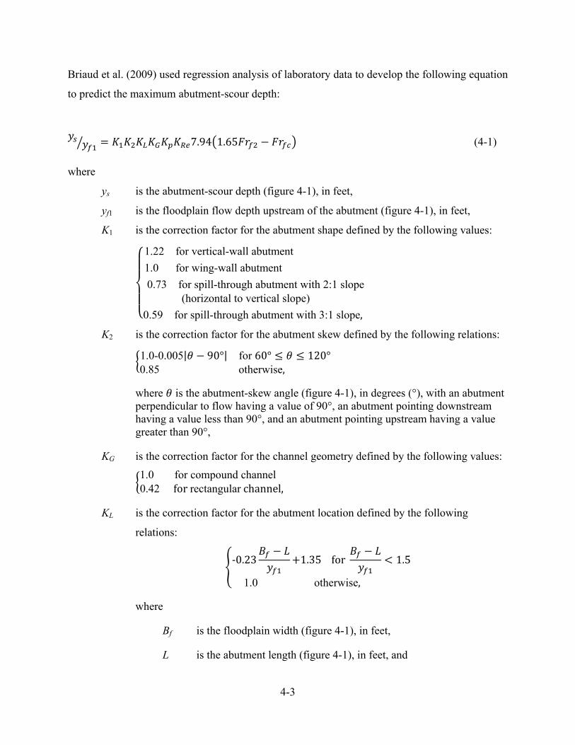
4-3
Briaud et al. (2009) used regression analysis of laboratory data to develop the following equation
to predict the maximum abutment-scour depth:
7.94 1.65 (4-1)
where
ys is the abutment-scour depth (figure 4-1), in feet,
yf1 is the floodplain flow depth upstream of the abutment (figure 4-1), in feet,
K1 is the correction factor for the abutment shape defined by the following values:
1.22 for vertical-wall abutment
1.0 for wing-wall abutment
0.73 for spill-through abutment with 2:1 slope(horizontal to vertical slope)
0.59 for spill-through abutment with 3:1 slope,
K2 is the correction factor for the abutment skew defined by the following relations:
1.0-0.005| 90°| for 60° 120°0.85 otherwise,
where is the abutment-skew angle (figure 4-1), in degrees (°), with an abutment perpendicular to flow having a value of 90°, an abutment pointing downstream having a value less than 90°, and an abutment pointing upstream having a value greater than 90°,
KG is the correction factor for the channel geometry defined by the following values:
1.0 for compound channel0.42 forrectangularchannel,
KL is the correction factor for the abutment location defined by the following
relations:
‐0.23 1.35for 1.5
1.0 otherwise,
where
Bf is the floodplain width (figure 4-1), in feet,
L is the abutment length (figure 4-1), in feet, and

4-4
yf1 is as previously defined,
Kp is the correction factor for pressure flow defined by the following relations:
0.92 / 1.0for / 1.00.21 / ‐1.27 / 2.97for1.0 / 3.01.0for3.0 / ,
where
d1 is the distance from water surface to the low chord of the bridge at
the upstream face of the bridge (figure 4-2), in feet, and
ddeck is the distance from high steel to the low chord of the bridge deck
blocking flow, in feet (figure 4-2),
KRe is the correction factor for the Reynolds number defined by the relation:
10.0327Re . ,
where
Ref2 is the Reynolds number around the abutment toe, equal to ,
where
ν is the kinematic viscosity of water (1.08x10⁻⁵ ft2/s at 20° Celsius),
and the other variables are as previously defined.
is the Froude number around the abutment toe, equal to ,
where
g is the acceleration due to gravity, in feet per second squared,
yf1 is as previously defined, and
Vf2 is the velocity around the toe of the abutment, in feet per second,
is the critical Froude number around the abutment toe, equal to ,
where
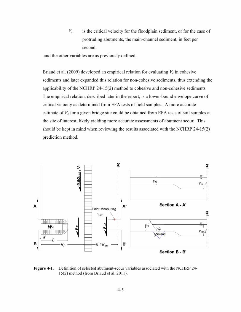
4-5
Vc is the critical velocity for the floodplain sediment, or for the case of
protruding abutments, the main-channel sediment, in feet per
second,
and the other variables are as previously defined.
Briaud et al. (2009) developed an empirical relation for evaluating Vc in cohesive
sediments and later expanded this relation for non-cohesive sediments, thus extending the
applicability of the NCHRP 24-15(2) method to cohesive and non-cohesive sediments.
The empirical relation, described later in the report, is a lower-bound envelope curve of
critical velocity as determined from EFA tests of field samples. A more accurate
estimate of Vc for a given bridge site could be obtained from EFA tests of soil samples at
the site of interest, likely yielding more accurate assessments of abutment scour. This
should be kept in mind when reviewing the results associated with the NCHRP 24-15(2)
prediction method.
Figure 4-1. Definition of selected abutment-scour variables associated with the NCHRP 24-15(2) method (from Briaud et al. 2011).
L Bf 0.5Bmc
ymc1
ymc1
ymc2
yf1
yf2
4-6
Figure 4-2. Definition of variables associated with pressure flow (from Briaud et al. 2011).

4-7
4.3 General Procedure for Application of NCHRP 24-15(2) to the
Laboratory and the USGS Field Data
Briaud et al. (2011) provide guidance for applying equation 4-1. As with any scour prediction
equation, some judgment is required in its application; therefore, a brief review of the steps used
in applying the NCHRP 24-15(2) method to the laboratory and USGS field data follows.
1. Compile laboratory and USGS field data
The laboratory and USGS field data previously described (tables 1-1 and 1-3) were
reviewed, and pertinent data for the NCHRP 24-15(2) method were entered into a
spreadsheet. These data included selected hydraulic, sediment, and bridge-geometry
characteristics as described in table 2-1.
2. Determine the correction factors for the abutment of interest
For most sites, the correction factors in equation 4-1 could be readily determined.
However, some sites had characteristics differing from those of the laboratory models
used in NCHRP 24-15(2) and required some judgment in determining the correction
factors. The Reynolds number correction factor uses hydraulic properties and is
discussed in item 8 below. Comments regarding the determination of the other correction
factor follow.
K1
Vertical-wall and wing-wall abutments have abutment-shape correction factors
with values of 1.22 and 1.0, respectively. (Note: No vertical-wall abutments were
in the field data.) For spill-through abutments, there are two possible abutment-
shape correction factors, 0.73 and 0.59, for spill-through slopes of 2:1 and 3:1,
respectively. Most of the laboratory and field data have spill-through slopes of
2:1 or steeper. For spill-through slopes steeper than 2:1, a correction factor value
of 0.73 was assumed. Additionally, where a spill-through slope was not provided
in the database, the site was assumed to have a slope of 2:1 or steeper.
4-8
K2
The abutment-skew correction factor can be readily determined from the relations
presented in equation 4-1, and no special consideration was required.
KG
The correction factor for channel geometry only has two cases, rectangular and
compound channels. For the laboratory data, the channel-geometry classification
is clearly specified and the values of KG can be readily determined. For the field
data, some judgment is required to determine the channel-geometry classification.
Sites with well-defined channels were classified as compound channels.
Floodplain relief bridges and swamps with poorly defined channels were
classified as rectangular channels.
KL
The abutment-location correction factor accounts for increased turbulence and
scour when the abutment toe is located near the channel bank. The largest value
for this correction factor (1.35) occurs when the abutment toe is located at the
channel bank. For most cases, the abutment-location correction factor can be
readily determined from the relations presented in equation 4-1. However, the
NCHRP 24-15(2) method did not evaluate the case for an abutment protruding
into the main channel. In such cases, the maximum abutment-location correction
factor of 1.35 was assumed to be applicable. Some sites had very small abutment
setbacks of approximately 2 ft or less. In such cases, it was assumed that the
abutment was set at the channel bank, and KL was assigned a value of 1.35.
Kp
The pressure-flow correction factor can be readily determined from the relations
presented in equation 4-1. No pressure-flow cases are in the laboratory data. In
contrast, some pressure-flow sites are in the USGS field data. These sites had
limited data regarding the bridge deck geometry, and this information was used to
approximate the variables (d1 and ddeck, figure 4-2) required for evaluating the
pressure-flow correction factor.
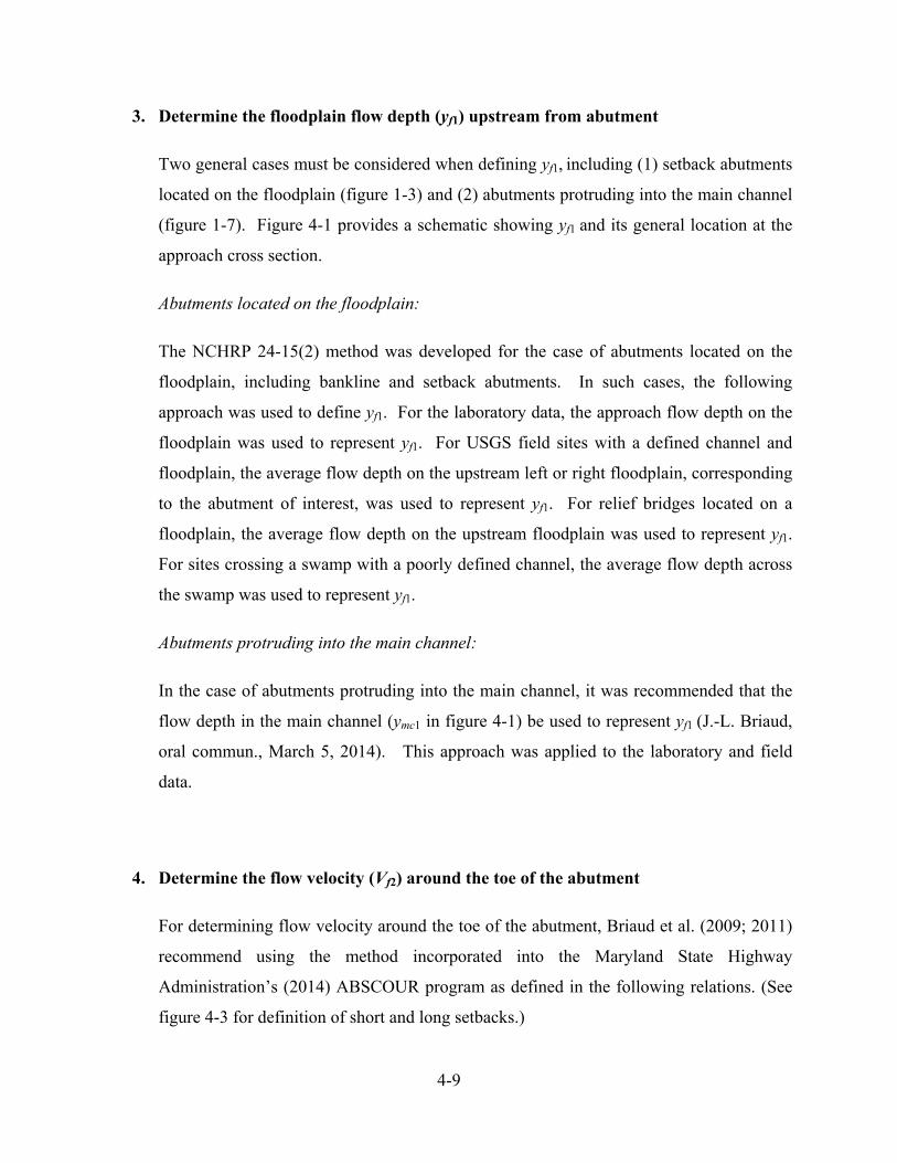
4-9
3. Determine the floodplain flow depth (yf1) upstream from abutment
Two general cases must be considered when defining yf1, including (1) setback abutments
located on the floodplain (figure 1-3) and (2) abutments protruding into the main channel
(figure 1-7). Figure 4-1 provides a schematic showing yf1 and its general location at the
approach cross section.
Abutments located on the floodplain:
The NCHRP 24-15(2) method was developed for the case of abutments located on the
floodplain, including bankline and setback abutments. In such cases, the following
approach was used to define yf1. For the laboratory data, the approach flow depth on the
floodplain was used to represent yf1. For USGS field sites with a defined channel and
floodplain, the average flow depth on the upstream left or right floodplain, corresponding
to the abutment of interest, was used to represent yf1. For relief bridges located on a
floodplain, the average flow depth on the upstream floodplain was used to represent yf1.
For sites crossing a swamp with a poorly defined channel, the average flow depth across
the swamp was used to represent yf1.
Abutments protruding into the main channel:
In the case of abutments protruding into the main channel, it was recommended that the
flow depth in the main channel (ymc1 in figure 4-1) be used to represent yf1 (J.-L. Briaud,
oral commun., March 5, 2014). This approach was applied to the laboratory and field
data.
4. Determine the flow velocity (Vf2) around the toe of the abutment
For determining flow velocity around the toe of the abutment, Briaud et al. (2009; 2011)
recommend using the method incorporated into the Maryland State Highway
Administration’s (2014) ABSCOUR program as defined in the following relations. (See
figure 4-3 for definition of short and long setbacks.)
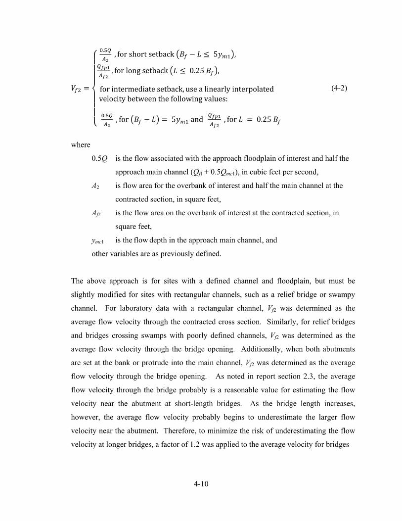
4-10
. , forshortsetback 5 ,
, forlongsetback 0.25 ,
forintermediatesetback, usealinearlyinterpolatedvelocitybetweenthefollowingvalues:
. , for 5 and , for 0.25
(4-2)
where
0.5Q is the flow associated with the approach floodplain of interest and half the
approach main channel (Qf1 + 0.5Qmc1), in cubic feet per second,
A2 is flow area for the overbank of interest and half the main channel at the
contracted section, in square feet,
Af2 is the flow area on the overbank of interest at the contracted section, in
square feet,
ymc1 is the flow depth in the approach main channel, and
other variables are as previously defined.
The above approach is for sites with a defined channel and floodplain, but must be
slightly modified for sites with rectangular channels, such as a relief bridge or swampy
channel. For laboratory data with a rectangular channel, Vf2 was determined as the
average flow velocity through the contracted cross section. Similarly, for relief bridges
and bridges crossing swamps with poorly defined channels, Vf2 was determined as the
average flow velocity through the bridge opening. Additionally, when both abutments
are set at the bank or protrude into the main channel, Vf2 was determined as the average
flow velocity through the bridge opening. As noted in report section 2.3, the average
flow velocity through the bridge probably is a reasonable value for estimating the flow
velocity near the abutment at short-length bridges. As the bridge length increases,
however, the average flow velocity probably begins to underestimate the larger flow
velocity near the abutment. Therefore, to minimize the risk of underestimating the flow
velocity at longer bridges, a factor of 1.2 was applied to the average velocity for bridges
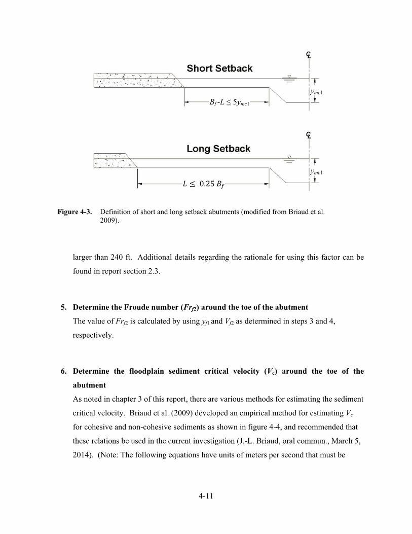
4-11
Figure 4-3. Definition of short and long setback abutments (modified from Briaud et al.
2009).
larger than 240 ft. Additional details regarding the rationale for using this factor can be
found in report section 2.3.
5. Determine the Froude number (Frf2) around the toe of the abutment
The value of Frf2 is calculated by using yf1 and Vf2 as determined in steps 3 and 4,
respectively.
6. Determine the floodplain sediment critical velocity (Vc) around the toe of the
abutment
As noted in chapter 3 of this report, there are various methods for estimating the sediment
critical velocity. Briaud et al. (2009) developed an empirical method for estimating Vc
for cohesive and non-cohesive sediments as shown in figure 4-4, and recommended that
these relations be used in the current investigation (J.-L. Briaud, oral commun., March 5,
2014). (Note: The following equations have units of meters per second that must be
Bf -L ≤ 5ymc1
0.25
ymc1
ymc1

4-12
converted to feet per second.) For sediments having a D50 greater than or equal to 0.1
mm, the following equation was used:
Vc = 0.35 D500.45, (4-3)
where
Vc is the sediment critical velocity, in meters per second, and
D50 is the median grain size for the sediment, in millimeters.
For sediments having a D50 less than 0.1 mm, the lower-bound equation in figure 4-4, as
follows, was used:
Vc = 0.1 D50-0.2, (4-4)
where all variables are as previously defined. A D50 representative of the floodplain or
main-channel sediments was used at floodplain setback abutments and protruding
abutments, respectively. The relation in figure 4-4 is a lower-bound curve of critical
velocity as determined from EFA tests of field samples. A more accurate estimate of Vc
for a given bridge site could be obtained from EFA tests of soil samples at the site of
interest, likely yielding more accurate assessments of abutment scour. This should be
kept in mind when reviewing the results associated with the NCHRP 24-15(2) prediction
method.
7. Determine the critical Froude number (Frfc) around the toe of the abutment
The value of Frfc is calculated by using yf1 and Vc as determined in steps 3 and 6,
respectively.
8. Determine the Reynolds number correction factor (KRe) around the toe of the
abutment
The value of Ref2 is calculated by using yf1 and Vf2 as determined in steps 3 and 4,
respectively. This value is then used in the relation for computing KRe as described in
equation 4-1.
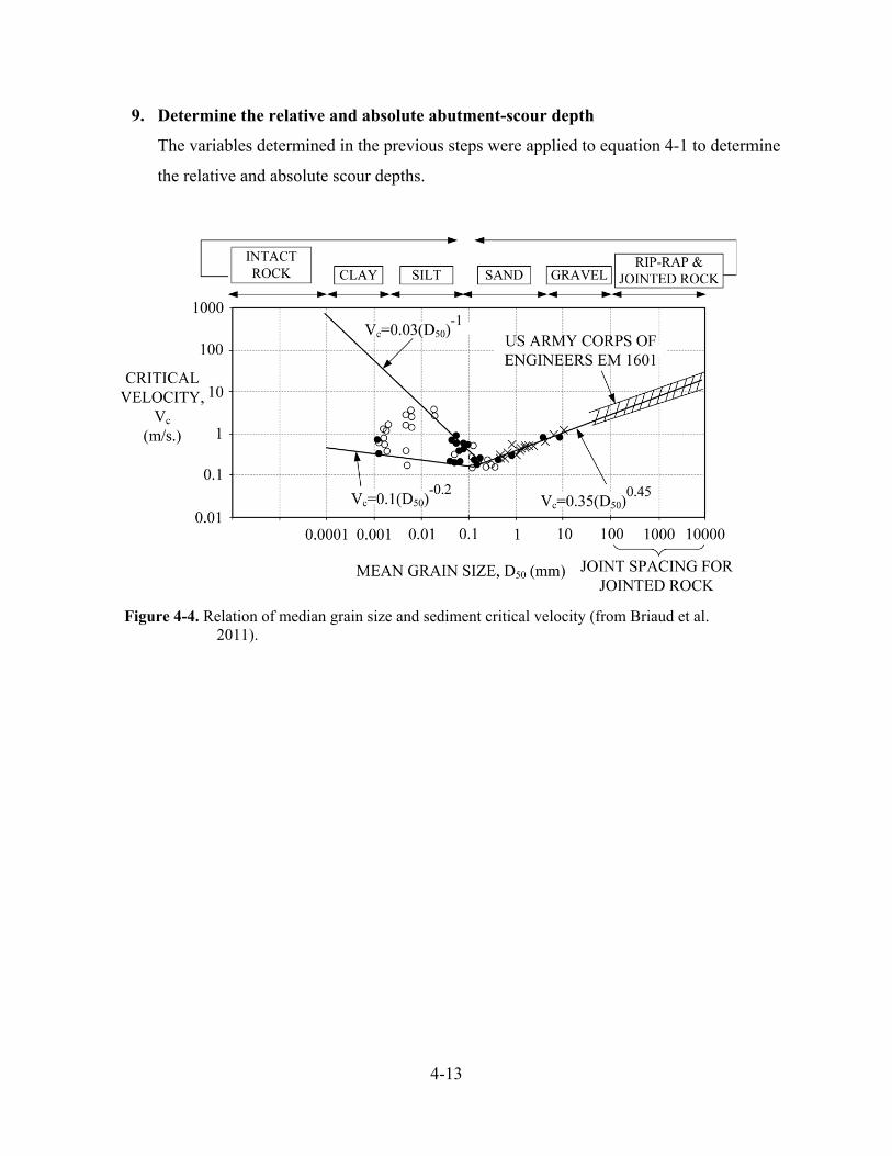
4-13
9. Determine the relative and absolute abutment-scour depth
The variables determined in the previous steps were applied to equation 4-1 to determine
the relative and absolute scour depths.
Figure 4-4. Relation of median grain size and sediment critical velocity (from Briaud et al. 2011).
5-1
CHAPTER 5
APPLICATION OF THE NCHRP 24-15(2) PREDICTION
METHOD TO LABORATORY AND FIELD DATA
5.1 Introduction
The NCHRP 24-15(2) abutment-scour prediction method was originally developed for predicting
abutment scour in cohesive sediments, but was extended to include abutment scour in non-
cohesive sediments (Briaud et al. 2009; 2011). The NCHRP 24-15(2) method provides two
procedures for predicting abutment scour, including (1) a time-dependent estimate requiring
detailed site information (primarily for cohesive sediments) that provides a refined estimate of
scour, and (2) the maximum scour depth estimate requiring less detailed data (for cohesive and
non-cohesive sediments). Briaud et al. (2009; 2011) note that currently no laboratory or field
abutment-scour databases include the detailed data required to evaluate the time-dependent
method in cohesive sediments. Therefore, any performance evaluation of the NCHRP 24-15(2)
abutment-scour prediction method with existing laboratory and field data must be limited to use
of the maximum scour-depth equation. This was the approach used in the current (2015)
investigation, and this limitation should be kept in mind when evaluating the results in this
report. The maximum scour-depth equation was originally developed for predicting abutment
scour in cohesive sediments by using an empirical relation for evaluating the sediment critical
velocity for cohesive sediments. This empirical relation for sediment critical velocity was later
expanded for non-cohesive sediments (see figure 4-4), thus extending the applicability of the
NCHRP 24-15(2) method to cohesive and non-cohesive sediments. Therefore, cohesive and
non-cohesive data are used in the evaluation of the NCHRP 24-15(2) method.
The procedure described in chapter 4 was used to apply the NCHRP 24-15(2) abutment-scour
prediction method to the selected laboratory (table 1-3) and field (table 1-1) abutment-scour data.
The results from this application were incorporated into selected scatter plots to display the
relations of predicted and measured scour, as well as prediction residuals with respect to selected
5-2
explanatory variables. If a prediction equation is capturing the trends of the data, then the
relation of the predicted and measured scour will tend to follow the line of agreement, with
predicted scour increasing as measured scour increases. The relation of prediction residuals with
respect to an explanatory variable will help identify prediction bias associated with that variable.
If prediction residuals display a sloped trend with respect to a given explanatory variable, some
prediction bias with respect to that variable is likely. Boxplots of the prediction residuals for the
laboratory and field data are presented in chapter 6 and compared with the prediction residuals of
the NCHRP 24-20 method. The boxplots display the distribution of the prediction residuals by
quartiles, providing a simple but useful tool for evaluating the performance of each method and
comparing their performance. A table of summary statistics for these boxplots also is provided in
chapter 6 in order to quantify the trends in the boxplots.
The performance of the NCHRP 24-15(2) maximum scour-depth equation presented in the
following sections of this report represents the combined influence of the equation, the
prescribed application procedure, and the data, each having inherent limitations. These
limitations will undoubtedly introduce uncertainty into the results; however, the larger number of
laboratory (table 1-3) and field (table 1-1) data should be adequate to provide valuable insights
into the general performance of the equation. The results associated with the laboratory data are
presented first, followed by the results of the field data.
5.2 Analysis of the Laboratory Data
The NCHRP 24-15(2) method was initially evaluated with the laboratory measurements of
abutment scour listed in table 1-3. The analysis included a comparison of predicted and
measured scour, an evaluation of the relative influence of selected variables in the NCHRP 24-
15(2) equation (equation 4-1) on predicted scour, and an evaluation of prediction residuals with
respect to selected equation variables. The analysis of the laboratory data is presented in the
following report sections.
5-3
5.2.1 Relation of Measured and Predicted Scour
Figure 5-1A shows the relation of measured abutment-scour depth to predicted scour for the
application of the NCHRP 24-15(2) method to the laboratory data listed in table 1-3. (For
clarity, a truncated portion of the graph in figure 5-1A is shown in figure 5-1B.) The data in
figure 5-1 are grouped by data source, abutment shape, and bed transport condition. Live-bed
scour conditions are represented by the solid symbols, with hollow symbols representing clear-
water scour conditions. The Palaviccini (1993) data are associated with rectangular channels,
while the other data, with a few exceptions [5 data points in Briaud et al. (2009) and 12 in
Ettema et al. (2010)], are associated with compound channels. The Briaud et al. (2009) data are
associated with cohesive sediments, while the other laboratory data represent non-cohesive
sediments. The laboratory data in figure 5-1 represent abutment scour from a variety of
experimental conditions; therefore, the scatter displayed in the data is not unreasonable. To
provide insights into equation performance with respect to abutment shape, figures 5-2 through
5-4 present the data grouped by abutment shape, including vertical-wall, spill-through, and wing-
wall abutments, respectively. Additionally, data are grouped by live-bed and clear-water scour
conditions in figures 5-5 and 5-6 to provide insights into equation performance with respect to
bed transport conditions. Some notable trends in these figures include:
The largest overpredictions for the Sturm (2004) data (3 data points in figure 5-2 and 2
data points in figure 5-3) and the Ettema et al. (2010) data (5 data points in figure 5-3 and
4 data points in figure 5-4) are associated with abutments located at the channel bank or
that protrude into the main channel. The abutment-location correction factor (KL) in
equation 4-1 for these types of abutments is 1.35, which will produce larger values of
predicted scour depth. A more detailed analysis of these data is presented later in this
chapter.
The live-bed data tend to produce larger overpredictions, particularly in the Palaviccini
(1993) vertical-wall abutment data (figures 5-1 and 5-5). As noted later, the live-bed data
often have large Froude numbers at the abutment (Frf2) which tend to produce larger
scour predictions when applied in equation 4-1. As previously noted, the Ettema et al.
5-4
(2010) live-bed data (figures 5-3 and 5-4) are associated with bankline or protruding
abutments that also contribute to the larger scour predictions for these data.
A review of figure 5-4 shows that three of the wing-wall abutments for the Briaud et al.
(2009) data have overpredictions that are much larger than overpredictions for the other
data. These three data points are associated with compound channels where the channel-
geometry correction factor (KG) in equation 4-1 has a value of 1.0. In contrast, the other
five Briaud et al. (2009) data points that have smaller overpredictions that fall closer to
the line of agreement are associated with rectangular channels where KG has a value of
0.42 that substantially reduces the magnitude of predicted scour. (Note: Most of the other
data in figure 5-4 have rectangular channels with the exception of the Ettema et al. (2010)
live-bed data.) All of the Briaud et al. (2009) data in figure 5-4 have similar hydraulic
and geometric characteristics, with the primary difference being channel geometry. The
trends for the Briaud et al. (2009) data in this figure indicate that KG may not fully reflect
the scour processes associated with differing channel geometries. The KG correction
factor is evaluated in more detail later in this report.
A review of the live-bed and clear-water scour data (figures 5-5 and 5-6, respectively)
indicates that the clear-water scour data have a much higher incident of underprediction.
With only a few exceptions, the underpredictions are associated with rectangular
channels. The channel-geometry correction factor (KG) in equation 4-1 for rectangular
channels is 0.42, which contributes to the underpredictions associated with these data.
Additionally, the clear-water data often have smaller Froude numbers at the abutment,
which tend to produce smaller scour predictions when applied in equation 4-1. A more
detailed analysis of these data is presented later in this chapter.
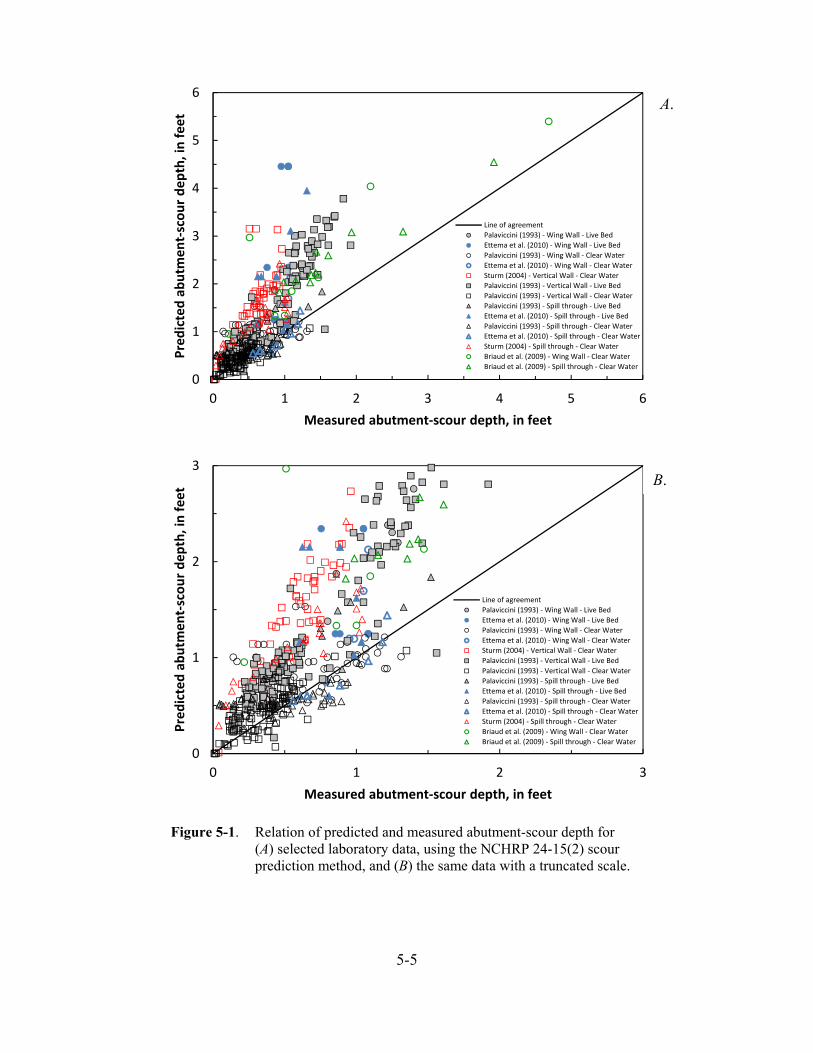
5-5
0
1
2
3
0 1 2 3
Predicted abutm
ent‐scour depth, in feet
Measured abutment‐scour depth, in feet
Line of agreement
Palaviccini (1993) ‐ Wing Wall ‐ Live Bed
Ettema et al. (2010) ‐ Wing Wall ‐ Live Bed
Palaviccini (1993) ‐ Wing Wall ‐ Clear Water
Ettema et al. (2010) ‐ Wing Wall ‐ Clear Water
Sturm (2004) ‐ Vertical Wall ‐ Clear Water
Palaviccini (1993) ‐ Vertical Wall ‐ Live Bed
Palaviccini (1993) ‐ Vertical Wall ‐ Clear Water
Palaviccini (1993) ‐ Spill through ‐ Live Bed
Ettema et al. (2010) ‐ Spill through ‐ Live Bed
Palaviccini (1993) ‐ Spill through ‐ Clear Water
Ettema et al. (2010) ‐ Spill through ‐ Clear Water
Sturm (2004) ‐ Spill through ‐ Clear Water
Briaud et al. (2009) ‐ Wing Wall ‐ Clear Water
Briaud et al. (2009) ‐ Spill through ‐ Clear Water
0
1
2
3
4
5
6
0 1 2 3 4 5 6
Predicted abutm
ent‐scour depth, in feet
Measured abutment‐scour depth, in feet
Line of agreement
Palaviccini (1993) ‐ Wing Wall ‐ Live Bed
Ettema et al. (2010) ‐ Wing Wall ‐ Live Bed
Palaviccini (1993) ‐ Wing Wall ‐ Clear Water
Ettema et al. (2010) ‐ Wing Wall ‐ Clear Water
Sturm (2004) ‐ Vertical Wall ‐ Clear Water
Palaviccini (1993) ‐ Vertical Wall ‐ Live Bed
Palaviccini (1993) ‐ Vertical Wall ‐ Clear Water
Palaviccini (1993) ‐ Spill through ‐ Live Bed
Ettema et al. (2010) ‐ Spill through ‐ Live Bed
Palaviccini (1993) ‐ Spill through ‐ Clear Water
Ettema et al. (2010) ‐ Spill through ‐ Clear Water
Sturm (2004) ‐ Spill through ‐ Clear Water
Briaud et al. (2009) ‐ Wing Wall ‐ Clear Water
Briaud et al. (2009) ‐ Spill through ‐ Clear Water
A.
B.
Figure 5-1. Relation of predicted and measured abutment-scour depth for (A) selected laboratory data, using the NCHRP 24-15(2) scour prediction method, and (B) the same data with a truncated scale.
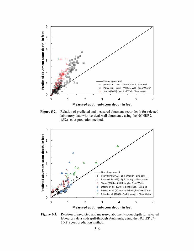
5-6
0
1
2
3
4
5
6
0 1 2 3 4 5 6
Predicted abutm
ent‐scour depth, in feet
Measured abutment‐scour depth, in feet
Line of agreement
Palaviccini (1993) ‐ Spill through ‐ Live Bed
Palaviccini (1993) ‐ Spill through ‐ Clear Water
Sturm (2004) ‐ Spill through ‐ Clear Water
Ettema et al. (2010) ‐ Spill through ‐ Live Bed
Ettema et al. (2010) ‐ Spill through ‐ Clear Water
Briaud et al. (2009) – Spill through – Clear Water
0
1
2
3
4
5
6
0 1 2 3 4 5 6
Predicted abutm
ent‐scour depth, in feet
Measured abutment‐scour depth, in feet
Line of agreement
Palaviccini (1993) ‐ Vertical Wall ‐ Live Bed
Palaviccini (1993) ‐ Vertical Wall ‐ Clear Water
Sturm (2004) ‐ Vertical Wall ‐ Clear Water
Figure 5-2. Relation of predicted and measured abutment-scour depth for selected laboratory data with vertical-wall abutments, using the NCHRP 24-15(2) scour prediction method.
Figure 5-3. Relation of predicted and measured abutment-scour depth for selected laboratory data with spill-through abutments, using the NCHRP 24-15(2) scour prediction method.
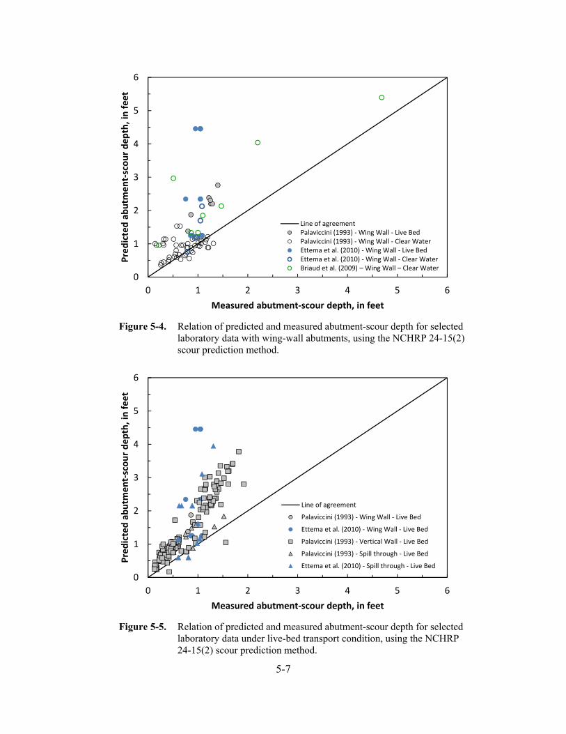
5-7
0
1
2
3
4
5
6
0 1 2 3 4 5 6
Predicted abutm
ent‐scour depth, in feet
Measured abutment‐scour depth, in feet
Line of agreementPalaviccini (1993) ‐ Wing Wall ‐ Live BedPalaviccini (1993) ‐ Wing Wall ‐ Clear WaterEttema et al. (2010) ‐ Wing Wall ‐ Live BedEttema et al. (2010) ‐ Wing Wall ‐ Clear WaterBriaud et al. (2009) – Wing Wall – Clear Water
0
1
2
3
4
5
6
0 1 2 3 4 5 6
Predicted abutm
ent‐scour depth, in feet
Measured abutment‐scour depth, in feet
Line of agreement
Palaviccini (1993) ‐ Wing Wall ‐ Live Bed
Ettema et al. (2010) ‐ Wing Wall ‐ Live Bed
Palaviccini (1993) ‐ Vertical Wall ‐ Live Bed
Palaviccini (1993) ‐ Spill through ‐ Live Bed
Ettema et al. (2010) ‐ Spill through ‐ Live Bed
Figure 5-4. Relation of predicted and measured abutment-scour depth for selected laboratory data with wing-wall abutments, using the NCHRP 24-15(2) scour prediction method.
Figure 5-5. Relation of predicted and measured abutment-scour depth for selected laboratory data under live-bed transport condition, using the NCHRP 24-15(2) scour prediction method.
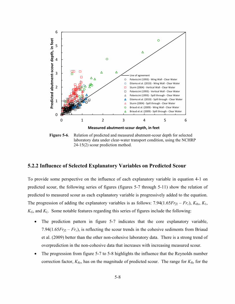
5-8
5.2.2 Influence of Selected Explanatory Variables on Predicted Scour
To provide some perspective on the influence of each explanatory variable in equation 4-1 on
predicted scour, the following series of figures (figures 5-7 through 5-11) show the relation of
predicted to measured scour as each explanatory variable is progressively added to the equation.
The progression of adding the explanatory variables is as follows: 7.94(1.65Frf2 – Frc), KRe, K1,
KG, and KL. Some notable features regarding this series of figures include the following:
The prediction pattern in figure 5-7 indicates that the core explanatory variable,
7.94(1.65Frf2 – Frc), is reflecting the scour trends in the cohesive sediments from Briaud
et al. (2009) better than the other non-cohesive laboratory data. There is a strong trend of
overprediction in the non-cohesive data that increases with increasing measured scour.
The progression from figure 5-7 to 5-8 highlights the influence that the Reynolds number
correction factor, KRe, has on the magnitude of predicted scour. The range for KRe for the
0
1
2
3
4
5
6
0 1 2 3 4 5 6
Predicted abutm
ent‐scour depth, in feet
Measured abutment‐scour depth, in feet
Line of agreement
Palaviccini (1993) ‐ Wing Wall ‐ Clear Water
Ettema et al. (2010) ‐ Wing Wall ‐ Clear Water
Sturm (2004) ‐ Vertical Wall ‐ Clear Water
Palaviccini (1993) ‐ Vertical Wall ‐ Clear Water
Palaviccini (1993) ‐ Spill through ‐ Clear Water
Ettema et al. (2010) ‐ Spill through ‐ Clear Water
Sturm (2004) ‐ Spill through ‐ Clear Water
Briaud et al. (2009) ‐ Wing Wall ‐ Clear Water
Briaud et al. (2009) ‐ Spill through ‐ Clear Water
Figure 5-6. Relation of predicted and measured abutment-scour depth for selected laboratory data under clear-water transport condition, using the NCHRP 24-15(2) scour prediction method.

5-9
laboratory data is from 0.9 to 2.5 with an average value of 1.58, indicating that KRe will
tend to increase predicted scour by about 60 percent on average.
The progression from figure 5-8 to 5-9 highlights the influence of K1 on predicted scour,
with vertical-wall abutments having increased predicted scour and spill-through
abutments having decreased predicted scour.
The progression from figure 5-9 to 5-10 highlights the influence of KG on predicted scour
for rectangular channels, substantially reducing the overprediction, but increasing the
frequency and magnitude of underprediction for such channels. All of the Palaviccini
(1993) data are associated with rectangular channels, and the influence of KG is strongly
displayed in these data.
The progression from figure 5-10 to 5-11 highlights the influence of KL on predicted
scour for bankline and protruding abutments, substantially increasing the overprediction
for such abutments. Additionally, the underprediction associated with bankline and
protruding abutments without the KL adjustment (figure 5-10) is infrequent, while
overprediction with the KL adjustment (figure 5-11) can be excessive at times. This
pattern indicates that KL is likely not critical in reducing underprediction at such
abutments. The KL correction factor is evaluated in more detail later in this report.
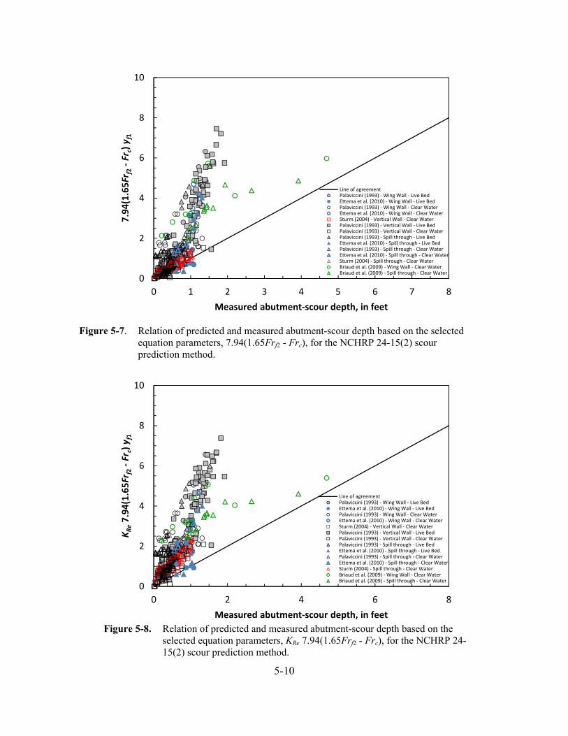
5-10
Figure 5-7. Relation of predicted and measured abutment-scour depth based on the selected equation parameters, 7.94(1.65Frf2 - Frc), for the NCHRP 24-15(2) scour prediction method.
0
2
4
6
8
10
0 2 4 6 8
KRe7.94(1.65Fr
f2‐Fr
c) y
f1
Measured abutment‐scour depth, in feet
Line of agreementPalaviccini (1993) ‐ Wing Wall ‐ Live BedEttema et al. (2010) ‐ Wing Wall ‐ Live BedPalaviccini (1993) ‐ Wing Wall ‐ Clear WaterEttema et al. (2010) ‐ Wing Wall ‐ Clear WaterSturm (2004) ‐ Vertical Wall ‐ Clear WaterPalaviccini (1993) ‐ Vertical Wall ‐ Live BedPalaviccini (1993) ‐ Vertical Wall ‐ Clear WaterPalaviccini (1993) ‐ Spill through ‐ Live BedEttema et al. (2010) ‐ Spill through ‐ Live BedPalaviccini (1993) ‐ Spill through ‐ Clear WaterEttema et al. (2010) ‐ Spill through ‐ Clear WaterSturm (2004) ‐ Spill through ‐ Clear WaterBriaud et al. (2009) ‐ Wing Wall ‐ Clear WaterBriaud et al. (2009) ‐ Spill through ‐ Clear Water
Figure 5-8. Relation of predicted and measured abutment-scour depth based on the selected equation parameters, KRe 7.94(1.65Frf2 - Frc), for the NCHRP 24-15(2) scour prediction method.
0
2
4
6
8
10
0 1 2 3 4 5 6 7 8
7.94(1.65Fr
f2‐Fr
c) y
f1
Measured abutment‐scour depth, in feet
Line of agreementPalaviccini (1993) ‐ Wing Wall ‐ Live BedEttema et al. (2010) ‐ Wing Wall ‐ Live BedPalaviccini (1993) ‐ Wing Wall ‐ Clear WaterEttema et al. (2010) ‐ Wing Wall ‐ Clear WaterSturm (2004) ‐ Vertical Wall ‐ Clear WaterPalaviccini (1993) ‐ Vertical Wall ‐ Live BedPalaviccini (1993) ‐ Vertical Wall ‐ Clear WaterPalaviccini (1993) ‐ Spill through ‐ Live BedEttema et al. (2010) ‐ Spill through ‐ Live BedPalaviccini (1993) ‐ Spill through ‐ Clear WaterEttema et al. (2010) ‐ Spill through ‐ Clear WaterSturm (2004) ‐ Spill through ‐ Clear WaterBriaud et al. (2009) ‐ Wing Wall ‐ Clear WaterBriaud et al. (2009) ‐ Spill through ‐ Clear Water
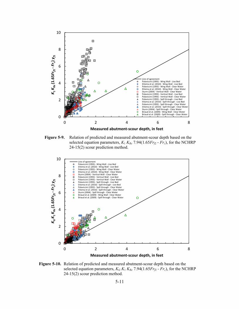
5-11
0
2
4
6
8
10
0 2 4 6 8
KG K
1KRe (1.65Fr
f2 ‐Fr
c) y
f1
Measured abutment‐scour depth, in feet
Line of agreementPalaviccini (1993) ‐ Wing Wall ‐ Live BedEttema et al. (2010) ‐ Wing Wall ‐ Live BedPalaviccini (1993) ‐ Wing Wall ‐ Clear WaterEttema et al. (2010) ‐ Wing Wall ‐ Clear WaterSturm (2004) ‐ Vertical Wall ‐ Clear WaterPalaviccini (1993) ‐ Vertical Wall ‐ Live BedPalaviccini (1993) ‐ Vertical Wall ‐ Clear WaterPalaviccini (1993) ‐ Spill through ‐ Live BedEttema et al. (2010) ‐ Spill through ‐ Live BedPalaviccini (1993) ‐ Spill through ‐ Clear WaterEttema et al. (2010) ‐ Spill through ‐ Clear WaterSturm (2004) ‐ Spill through ‐ Clear WaterBriaud et al. (2009) ‐ Wing Wall ‐ Clear WaterBriaud et al. (2009) ‐ Spill through ‐ Clear Water
Figure 5-10. Relation of predicted and measured abutment-scour depth based on the selected equation parameters, KG K1 KRe 7.94(1.65Frf2 - Frc), for the NCHRP 24-15(2) scour prediction method.
0
2
4
6
8
10
0 2 4 6 8
K1KRe (1.65Fr
f2 ‐Fr
c) y
f1
Measured abutment‐scour depth, in feet
Line of agreementPalaviccini (1993) ‐ Wing Wall ‐ Live BedEttema et al. (2010) ‐ Wing Wall ‐ Live BedPalaviccini (1993) ‐ Wing Wall ‐ Clear WaterEttema et al. (2010) ‐ Wing Wall ‐ Clear WaterSturm (2004) ‐ Vertical Wall ‐ Clear WaterPalaviccini (1993) ‐ Vertical Wall ‐ Live BedPalaviccini (1993) ‐ Vertical Wall ‐ Clear WaterPalaviccini (1993) ‐ Spill through ‐ Live BedEttema et al. (2010) ‐ Spill through ‐ Live BedPalaviccini (1993) ‐ Spill through ‐ Clear WaterEttema et al. (2010) ‐ Spill through ‐ Clear WaterSturm (2004) ‐ Spill through ‐ Clear WaterBriaud et al. (2009) ‐ Wing Wall ‐ Clear WaterBriaud et al. (2009) ‐ Spill through ‐ Clear Water
Figure 5-9. Relation of predicted and measured abutment-scour depth based on the selected equation parameters, K1 KRe 7.94(1.65Frf2 - Frc), for the NCHRP 24-15(2) scour prediction method.
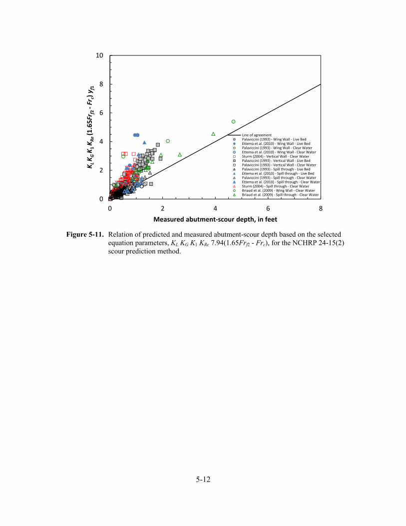
5-12
0
2
4
6
8
10
0 2 4 6 8
KL KG K
1KRe (1.65Fr
f2 ‐Fr
c) y
f1
Measured abutment‐scour depth, in feet
Line of agreementPalaviccini (1993) ‐ Wing Wall ‐ Live BedEttema et al. (2010) ‐ Wing Wall ‐ Live BedPalaviccini (1993) ‐ Wing Wall ‐ Clear WaterEttema et al. (2010) ‐ Wing Wall ‐ Clear WaterSturm (2004) ‐ Vertical Wall ‐ Clear WaterPalaviccini (1993) ‐ Vertical Wall ‐ Live BedPalaviccini (1993) ‐ Vertical Wall ‐ Clear WaterPalaviccini (1993) ‐ Spill through ‐ Live BedEttema et al. (2010) ‐ Spill through ‐ Live BedPalaviccini (1993) ‐ Spill through ‐ Clear WaterEttema et al. (2010) ‐ Spill through ‐ Clear WaterSturm (2004) ‐ Spill through ‐ Clear WaterBriaud et al. (2009) ‐ Wing Wall ‐ Clear WaterBriaud et al. (2009) ‐ Spill through ‐ Clear Water
Figure 5-11. Relation of predicted and measured abutment-scour depth based on the selected equation parameters, KL KG K1 KRe 7.94(1.65Frf2 - Frc), for the NCHRP 24-15(2) scour prediction method.
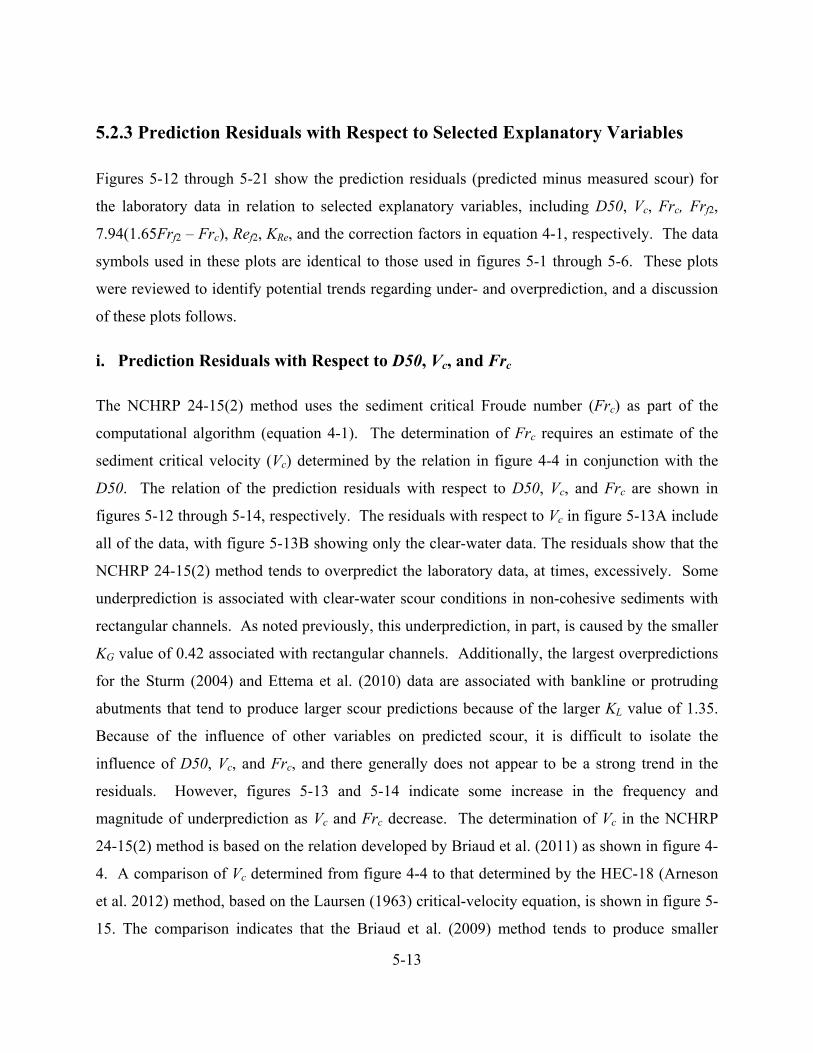
5-13
5.2.3 Prediction Residuals with Respect to Selected Explanatory Variables
Figures 5-12 through 5-21 show the prediction residuals (predicted minus measured scour) for
the laboratory data in relation to selected explanatory variables, including D50, Vc, Frc, Frf2,
7.94(1.65Frf2 – Frc), Ref2, KRe, and the correction factors in equation 4-1, respectively. The data
symbols used in these plots are identical to those used in figures 5-1 through 5-6. These plots
were reviewed to identify potential trends regarding under- and overprediction, and a discussion
of these plots follows.
i. Prediction Residuals with Respect to D50, Vc, and Frc
The NCHRP 24-15(2) method uses the sediment critical Froude number (Frc) as part of the
computational algorithm (equation 4-1). The determination of Frc requires an estimate of the
sediment critical velocity (Vc) determined by the relation in figure 4-4 in conjunction with the
D50. The relation of the prediction residuals with respect to D50, Vc, and Frc are shown in
figures 5-12 through 5-14, respectively. The residuals with respect to Vc in figure 5-13A include
all of the data, with figure 5-13B showing only the clear-water data. The residuals show that the
NCHRP 24-15(2) method tends to overpredict the laboratory data, at times, excessively. Some
underprediction is associated with clear-water scour conditions in non-cohesive sediments with
rectangular channels. As noted previously, this underprediction, in part, is caused by the smaller
KG value of 0.42 associated with rectangular channels. Additionally, the largest overpredictions
for the Sturm (2004) and Ettema et al. (2010) data are associated with bankline or protruding
abutments that tend to produce larger scour predictions because of the larger KL value of 1.35.
Because of the influence of other variables on predicted scour, it is difficult to isolate the
influence of D50, Vc, and Frc, and there generally does not appear to be a strong trend in the
residuals. However, figures 5-13 and 5-14 indicate some increase in the frequency and
magnitude of underprediction as Vc and Frc decrease. The determination of Vc in the NCHRP
24-15(2) method is based on the relation developed by Briaud et al. (2011) as shown in figure 4-
4. A comparison of Vc determined from figure 4-4 to that determined by the HEC-18 (Arneson
et al. 2012) method, based on the Laursen (1963) critical-velocity equation, is shown in figure 5-
15. The comparison indicates that the Briaud et al. (2009) method tends to produce smaller
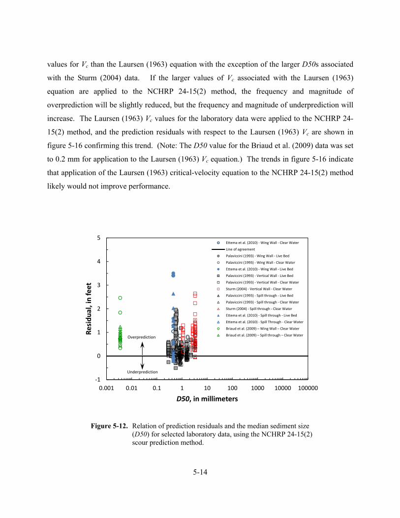
5-14
values for Vc than the Laursen (1963) equation with the exception of the larger D50s associated
with the Sturm (2004) data. If the larger values of Vc associated with the Laursen (1963)
equation are applied to the NCHRP 24-15(2) method, the frequency and magnitude of
overprediction will be slightly reduced, but the frequency and magnitude of underprediction will
increase. The Laursen (1963) Vc values for the laboratory data were applied to the NCHRP 24-
15(2) method, and the prediction residuals with respect to the Laursen (1963) Vc are shown in
figure 5-16 confirming this trend. (Note: The D50 value for the Briaud et al. (2009) data was set
to 0.2 mm for application to the Laursen (1963) Vc equation.) The trends in figure 5-16 indicate
that application of the Laursen (1963) critical-velocity equation to the NCHRP 24-15(2) method
likely would not improve performance.
Figure 5-12. Relation of prediction residuals and the median sediment size
(D50) for selected laboratory data, using the NCHRP 24-15(2) scour prediction method.
‐1
0
1
2
3
4
5
0.001 0.01 0.1 1 10 100 1000 10000 100000
Residual, in feet
D50, in millimeters
Ettema et al. (2010) ‐ Wing Wall ‐ Clear Water
Line of agreement
Palaviccini (1993) ‐ Wing Wall ‐ Live Bed
Palaviccini (1993) ‐ Wing Wall ‐ Clear Water
Ettema et al. (2010) ‐ Wing Wall ‐ Live Bed
Palaviccini (1993) ‐ Vertical Wall ‐ Live Bed
Palaviccini (1993) ‐ Vertical Wall ‐ Clear Water
Sturm (2004) ‐ Vertical Wall ‐ Clear Water
Palaviccini (1993) ‐ Spill through ‐ Live Bed
Palaviccini (1993) ‐ Spill through ‐ Clear Water
Sturm (2004) ‐ Spill through ‐ Clear Water
Ettema et al. (2010) ‐ Spill through ‐ Live Bed
Ettema et al. (2010) ‐ Spill Through ‐ Clear Water
Briaud et al. (2009) – Wing Wall – Clear Water
Briaud et al. (2009) – Spill through – Clear WaterOverprediction
Underprediction
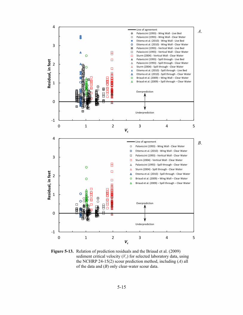
5-15
Figure 5-13. Relation of prediction residuals and the Briaud et al. (2009) sediment critical velocity (Vc) for selected laboratory data, using the NCHRP 24-15(2) scour prediction method, including (A) all of the data and (B) only clear-water scour data.
A.
B.
‐1
0
1
2
3
4
0 1 2 3 4 5
Residual, in feet
Vc
Line of agreement
Palaviccini (1993) ‐ Wing Wall ‐ Live Bed
Palaviccini (1993) ‐ Wing Wall ‐ Clear Water
Ettema et al. (2010) ‐ Wing Wall ‐ Live Bed
Ettema et al. (2010) ‐ Wing Wall ‐ Clear Water
Palaviccini (1993) ‐ Vertical Wall ‐ Live Bed
Palaviccini (1993) ‐ Vertical Wall ‐ Clear Water
Sturm (2004) ‐ Vertical Wall ‐ Clear Water
Palaviccini (1993) ‐ Spill through ‐ Live Bed
Palaviccini (1993) ‐ Spill through ‐ Clear Water
Sturm (2004) ‐ Spill through ‐ Clear Water
Ettema et al. (2010) ‐ Spill through ‐ Live Bed
Ettema et al. (2010) ‐ Spill through ‐ Clear Water
Briaud et al. (2009) – Wing Wall – Clear Water
Briaud et al. (2009) – Spill through – Clear Water
Overprediction
Underprediction
‐1
0
1
2
3
4
0 1 2 3 4 5
Residual, in feet
Vc
Line of agreement
Palaviccini (1993) ‐ Wing Wall ‐ Clear Water
Ettema et al. (2010) ‐ Wing Wall ‐ Clear Water
Palaviccini (1993) ‐ Vertical Wall ‐ Clear Water
Sturm (2004) ‐ Vertical Wall ‐ Clear Water
Palaviccini (1993) ‐ Spill through ‐ Clear Water
Sturm (2004) ‐ Spill through ‐ Clear Water
Ettema et al. (2010) ‐ Spill through ‐ Clear Water
Briaud et al. (2009) – Wing Wall – Clear Water
Briaud et al. (2009) – Spill through – Clear Water
Overprediction
Underprediction
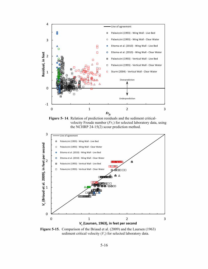
5-16
‐1
0
1
2
3
4
0 1 2 3
Residual, in feet
Frfc
Line of agreement
Palaviccini (1993) ‐ Wing Wall ‐ Live Bed
Palaviccini (1993) ‐ Wing Wall ‐ Clear Water
Ettema et al. (2010) ‐ Wing Wall ‐ Live Bed
Ettema et al. (2010) ‐ Wing Wall ‐ Clear Water
Palaviccini (1993) ‐ Vertical Wall ‐ Live Bed
Palaviccini (1993) ‐ Vertical Wall ‐ Clear Water
Sturm (2004) ‐ Vertical Wall ‐ Clear Water
Overprediction
Underprediction
0
1
2
3
0 1 2 3
Vc(Briau
d et al. 2009), in
feet per second
Vc (Laursen, 1963), in feet per second
Line of agreement
Palaviccini (1993) ‐ Wing Wall ‐ Live Bed
Palaviccini (1993) ‐ Wing Wall ‐ Clear Water
Ettema et al. (2010) ‐ Wing Wall ‐ Live Bed
Ettema et al. (2010) ‐ Wing Wall ‐ Clear Water
Palaviccini (1993) ‐ Vertical Wall ‐ Live Bed
Palaviccini (1993) ‐ Vertical Wall ‐ Clear Water
Figure 5- 14. Relation of prediction residuals and the sediment critical-velocity Froude number (Frc) for selected laboratory data, using the NCHRP 24-15(2) scour prediction method.
Figure 5-15. Comparison of the Briaud et al. (2009) and the Laursen (1963) sediment critical velocity (Vc) for selected laboratory data.
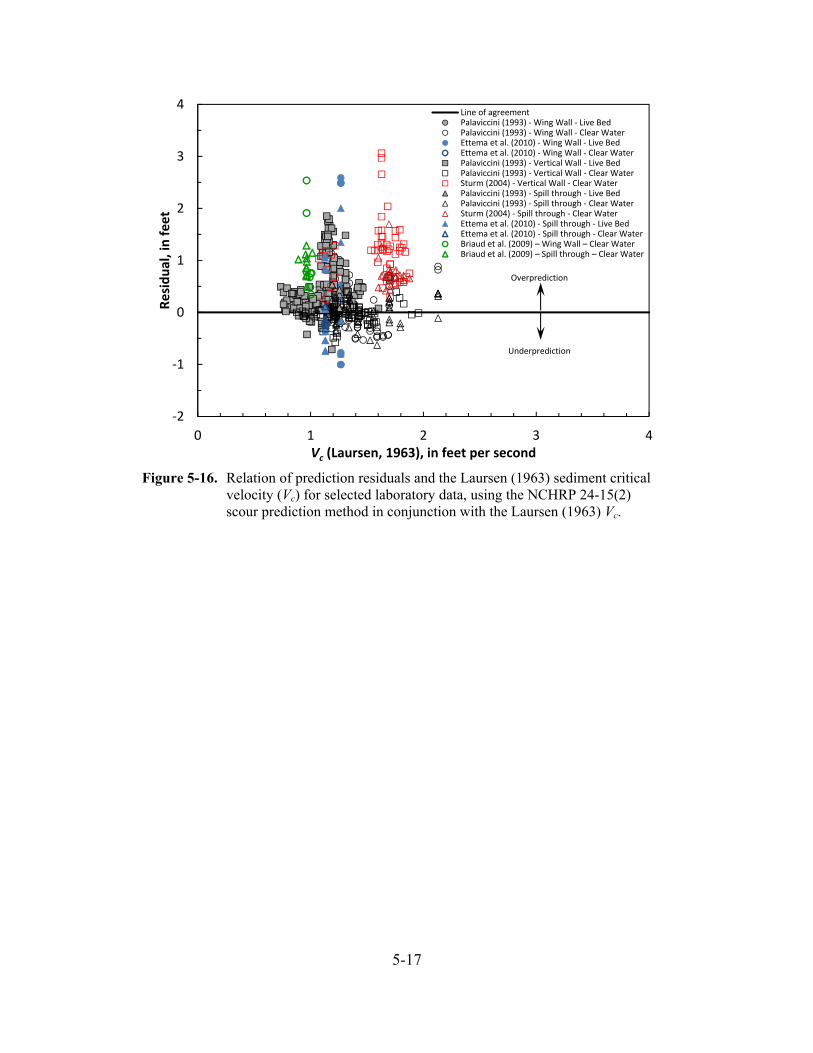
5-17
Figure 5-16. Relation of prediction residuals and the Laursen (1963) sediment critical velocity (Vc) for selected laboratory data, using the NCHRP 24-15(2) scour prediction method in conjunction with the Laursen (1963) Vc.
‐2
‐1
0
1
2
3
4
0 1 2 3 4
Residual, in feet
Vc (Laursen, 1963), in feet per second
Line of agreementPalaviccini (1993) ‐ Wing Wall ‐ Live BedPalaviccini (1993) ‐ Wing Wall ‐ Clear WaterEttema et al. (2010) ‐ Wing Wall ‐ Live BedEttema et al. (2010) ‐ Wing Wall ‐ Clear WaterPalaviccini (1993) ‐ Vertical Wall ‐ Live BedPalaviccini (1993) ‐ Vertical Wall ‐ Clear WaterSturm (2004) ‐ Vertical Wall ‐ Clear WaterPalaviccini (1993) ‐ Spill through ‐ Live BedPalaviccini (1993) ‐ Spill through ‐ Clear WaterSturm (2004) ‐ Spill through ‐ Clear WaterEttema et al. (2010) ‐ Spill through ‐ Live BedEttema et al. (2010) ‐ Spill through ‐ Clear WaterBriaud et al. (2009) – Wing Wall – Clear WaterBriaud et al. (2009) – Spill through – Clear Water
Overprediction
Underprediction
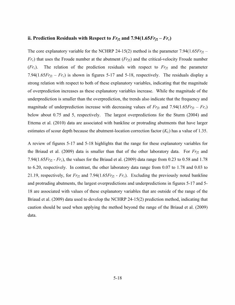
5-18
ii. Prediction Residuals with Respect to Frf2 and 7.94(1.65Frf2 – Frc)
The core explanatory variable for the NCHRP 24-15(2) method is the parameter 7.94(1.65Frf2 –
Frc) that uses the Froude number at the abutment (Frf2) and the critical-velocity Froude number
(Frc). The relation of the prediction residuals with respect to Frf2 and the parameter
7.94(1.65Frf2 – Frc) is shown in figures 5-17 and 5-18, respectively. The residuals display a
strong relation with respect to both of these explanatory variables, indicating that the magnitude
of overprediction increases as these explanatory variables increase. While the magnitude of the
underprediction is smaller than the overprediction, the trends also indicate that the frequency and
magnitude of underprediction increase with decreasing values of Frf2 and 7.94(1.65Frf2 – Frc)
below about 0.75 and 5, respectively. The largest overpredictions for the Sturm (2004) and
Ettema et al. (2010) data are associated with bankline or protruding abutments that have larger
estimates of scour depth because the abutment-location correction factor (KL) has a value of 1.35.
A review of figures 5-17 and 5-18 highlights that the range for these explanatory variables for
the Briaud et al. (2009) data is smaller than that of the other laboratory data. For Frf2 and
7.94(1.65Frf2 - Frc), the values for the Briaud et al. (2009) data range from 0.23 to 0.58 and 1.78
to 6.20, respectively. In contrast, the other laboratory data range from 0.07 to 1.78 and 0.03 to
21.19, respectively, for Frf2 and 7.94(1.65Frf2 - Frc). Excluding the previously noted bankline
and protruding abutments, the largest overpredictions and underpredictions in figures 5-17 and 5-
18 are associated with values of these explanatory variables that are outside of the range of the
Briaud et al. (2009) data used to develop the NCHRP 24-15(2) prediction method, indicating that
caution should be used when applying the method beyond the range of the Briaud et al. (2009)
data.
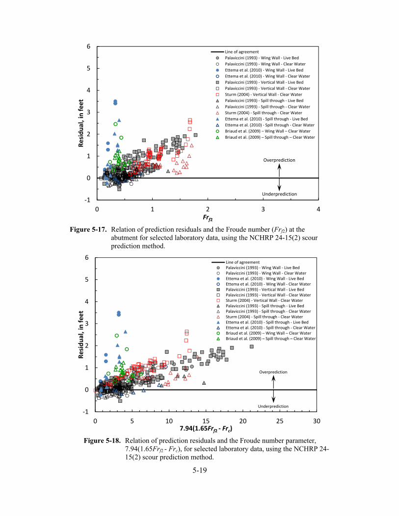
5-19
Figure 5-17. Relation of prediction residuals and the Froude number (Frf2) at the abutment for selected laboratory data, using the NCHRP 24-15(2) scour prediction method.
Figure 5-18. Relation of prediction residuals and the Froude number parameter, 7.94(1.65Frf2 - Frc), for selected laboratory data, using the NCHRP 24-15(2) scour prediction method.
‐1
0
1
2
3
4
5
6
0 1 2 3 4
Residual, in feet
Frf2
Line of agreement
Palaviccini (1993) ‐ Wing Wall ‐ Live Bed
Palaviccini (1993) ‐ Wing Wall ‐ Clear Water
Ettema et al. (2010) ‐ Wing Wall ‐ Live Bed
Ettema et al. (2010) ‐ Wing Wall ‐ Clear Water
Palaviccini (1993) ‐ Vertical Wall ‐ Live Bed
Palaviccini (1993) ‐ Vertical Wall ‐ Clear Water
Sturm (2004) ‐ Vertical Wall ‐ Clear Water
Palaviccini (1993) ‐ Spill through ‐ Live Bed
Palaviccini (1993) ‐ Spill through ‐ Clear Water
Sturm (2004) ‐ Spill through ‐ Clear Water
Ettema et al. (2010) ‐ Spill through ‐ Live Bed
Ettema et al. (2010) ‐ Spill through ‐ Clear Water
Briaud et al. (2009) – Wing Wall – Clear Water
Briaud et al. (2009) – Spill through – Clear Water
Overprediction
Underprediction
‐1
0
1
2
3
4
5
6
0 5 10 15 20 25 30
Residual, in feet
7.94(1.65Frf2 ‐ Frc)
Line of agreementPalaviccini (1993) ‐ Wing Wall ‐ Live BedPalaviccini (1993) ‐ Wing Wall ‐ Clear WaterEttema et al. (2010) ‐ Wing Wall ‐ Live BedEttema et al. (2010) ‐ Wing Wall ‐ Clear WaterPalaviccini (1993) ‐ Vertical Wall ‐ Live BedPalaviccini (1993) ‐ Vertical Wall ‐ Clear WaterSturm (2004) ‐ Vertical Wall ‐ Clear WaterPalaviccini (1993) ‐ Spill through ‐ Live BedPalaviccini (1993) ‐ Spill through ‐ Clear WaterSturm (2004) ‐ Spill through ‐ Clear WaterEttema et al. (2010) ‐ Spill through ‐ Live BedEttema et al. (2010) ‐ Spill through ‐ Clear WaterBriaud et al. (2009) – Wing Wall – Clear WaterBriaud et al. (2009) – Spill through – Clear Water
Overprediction
Underprediction

5-20
iii. Prediction Residuals with Respect to Ref2 and KRe
The NCHRP 24-15(2) method incorporates a correction factor for the Reynolds number at the
abutment (Ref2), expressed as KRe. In a literature review of previous investigations of abutment
scour, Sturm et al. (2011) provided a list of 19 selected abutment-scour prediction equations
developed during the period from 1961 to 2010. A review of these equations indicates that none,
with the exception of the NCHRP 24-15(2) equation, include the Reynolds number as an
explanatory variable. Melville and Coleman (2000) and Sturm et al. (2011) note that viscous
effects, as incorporated in the Reynolds number, can be neglected in the derivation of abutment-
and contraction-scour equations because of the large values for Reynolds numbers typically
associated with prototype turbulent flows. This provides some explanation for the absence of the
Reynolds number from the other abutment-scour equations, and suggests that its inclusion in the
NCHRP 24-15(2) method is problematic.
The relation of the prediction residuals with respect to Ref2 is shown in figure 5-19A, which
displays a trend indicating that the magnitude of overprediction increases as Ref2 increases.
While the magnitude of the underprediction is smaller than the overprediction, there is a similar
trend of increasing magnitude of underprediction with increasing Ref2. The Sturm (2004) data
have larger residuals than the other data within the same range of Ref2. This difference is
primarily attributed to the channel-geometry correction factor, KG, with the Sturm (2004) data
having compound channels with a KG value of 1.0 in contrast to most of the other data in the
same range of Ref2 and having rectangular channels with a KG value of 0.42. To highlight the
trend in the residuals, figure 5-19B shows the same data as in figure 5-19A without the Sturm
(2004) data. All of the Palaviccini (1993) data have rectangular channels with a common KG
value of 0.42, and the increased overprediction with increasing Ref2 is observable.
To provide perspective on how the Reynolds number correction factor KRe varies with Ref2,
figure 5-20 shows a plot of KRe with respect to arbitrary values of Ref2. The plot indicates that
KRe is inversely proportional to Ref2, decreasing as Ref2 increases. The range of Ref2 for the
Briaud et al. (2009) data, all of the laboratory data, and the field data are shown in the figure,
with Ref2 ranging from about 98,000 to 310,000 for the Briaud data, 7,000 to 310,000 for all of
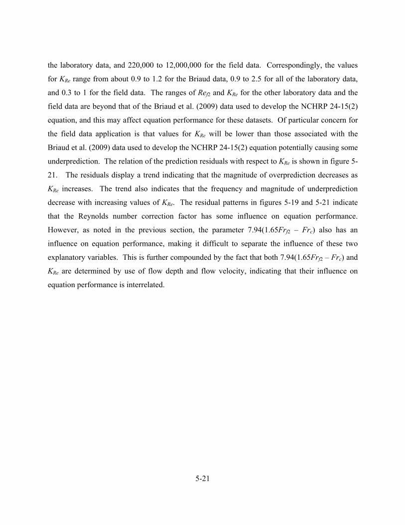
5-21
the laboratory data, and 220,000 to 12,000,000 for the field data. Correspondingly, the values
for KRe range from about 0.9 to 1.2 for the Briaud data, 0.9 to 2.5 for all of the laboratory data,
and 0.3 to 1 for the field data. The ranges of Ref2 and KRe for the other laboratory data and the
field data are beyond that of the Briaud et al. (2009) data used to develop the NCHRP 24-15(2)
equation, and this may affect equation performance for these datasets. Of particular concern for
the field data application is that values for KRe will be lower than those associated with the
Briaud et al. (2009) data used to develop the NCHRP 24-15(2) equation potentially causing some
underprediction. The relation of the prediction residuals with respect to KRe is shown in figure 5-
21. The residuals display a trend indicating that the magnitude of overprediction decreases as
KRe increases. The trend also indicates that the frequency and magnitude of underprediction
decrease with increasing values of KRe. The residual patterns in figures 5-19 and 5-21 indicate
that the Reynolds number correction factor has some influence on equation performance.
However, as noted in the previous section, the parameter 7.94(1.65Frf2 – Frc) also has an
influence on equation performance, making it difficult to separate the influence of these two
explanatory variables. This is further compounded by the fact that both 7.94(1.65Frf2 – Frc) and
KRe are determined by use of flow depth and flow velocity, indicating that their influence on
equation performance is interrelated.

5-22
Figure 5-19. Relation of prediction residuals and the Reynolds number at the abutment (Ref2) for selected laboratory data, using the NCHRP 24-15(2) scour prediction method, including (A) all of the data, and (B) without the Sturm (2004) data.
‐1
0
1
2
3
4
100 1,000 10,000 100,000
Residual, in feet
Re
Line of agreement
Palaviccini (1993) ‐ Wing Wall ‐ Live Bed
Palaviccini (1993) ‐ Wing Wall ‐ Clear Water
Ettema et al. (2010) ‐ Wing Wall ‐ Live Bed
Ettema et al. (2010) ‐ Wing Wall ‐ Clear Water
Palaviccini (1993) ‐ Vertical Wall ‐ Live Bed
Palaviccini (1993) ‐ Vertical Wall ‐ Clear Water
Palaviccini (1993) ‐ Spill through ‐ Live Bed
Palaviccini (1993) ‐ Spill through ‐ Clear Water
Ettema et al. (2010) ‐ Spill through ‐ Live Bed
Ettema et al. (2010) ‐ Spill through ‐ Clear Water
Briaud et al. (2009) – Wing Wall – Clear Water
Briaud et al. (2009) – Spill through – Clear Water
Overprediction
Underprediction
‐1
0
1
2
3
4
100 1,000 10,000 100,000
Residual, in feet
Re
Line of agreementPalaviccini (1993) ‐ Wing Wall ‐ Live BedPalaviccini (1993) ‐ Wing Wall ‐ Clear WaterEttema et al. (2010) ‐ Wing Wall ‐ Live BedEttema et al. (2010) ‐ Wing Wall ‐ Clear WaterPalaviccini (1993) ‐ Vertical Wall ‐ Live BedPalaviccini (1993) ‐ Vertical Wall ‐ Clear WaterSturm (2004) ‐ Vertical Wall ‐ Clear WaterPalaviccini (1993) ‐ Spill through ‐ Live BedPalaviccini (1993) ‐ Spill through ‐ Clear WaterSturm (2004) ‐ Spill through ‐ Clear WaterEttema et al. (2010) ‐ Spill through ‐ Live BedEttema et al. (2010) ‐ Spill through ‐ Clear WaterBriaud et al. (2009) – Wing Wall – Clear WaterBriaud et al. (2009) – Spill through – Clear Water
Overprediction
Underprediction
A.
B.
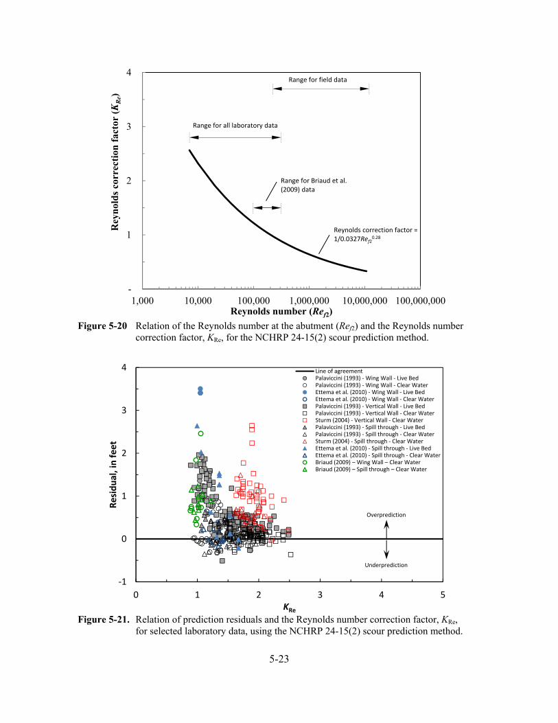
5-23
Figure 5-21. Relation of prediction residuals and the Reynolds number correction factor, KRe, for selected laboratory data, using the NCHRP 24-15(2) scour prediction method.
-
1
2
3
4
1,000 10,000 100,000 1,000,000 10,000,000 100,000,000
Rey
nol
ds
corr
ecti
on f
acto
r (K
Re)
Reynolds number (Ref2)
Range for Briaud et al. (2009) data
Range for all laboratory data
Range for field data
Reynolds correction factor = 1/0.0327Ref2
0.28
Figure 5-20 Relation of the Reynolds number at the abutment (Ref2) and the Reynolds number correction factor, KRe, for the NCHRP 24-15(2) scour prediction method.
‐1
0
1
2
3
4
0 1 2 3 4 5
Residual, in feet
KRe
Line of agreementPalaviccini (1993) ‐ Wing Wall ‐ Live BedPalaviccini (1993) ‐ Wing Wall ‐ Clear WaterEttema et al. (2010) ‐ Wing Wall ‐ Live BedEttema et al. (2010) ‐ Wing Wall ‐ Clear WaterPalaviccini (1993) ‐ Vertical Wall ‐ Live BedPalaviccini (1993) ‐ Vertical Wall ‐ Clear WaterSturm (2004) ‐ Vertical Wall ‐ Clear WaterPalaviccini (1993) ‐ Spill through ‐ Live BedPalaviccini (1993) ‐ Spill through ‐ Clear WaterSturm (2004) ‐ Spill through ‐ Clear WaterEttema et al. (2010) ‐ Spill through ‐ Live BedEttema et al. (2010) ‐ Spill through ‐ Clear WaterBriaud (2009) – Wing Wall – Clear WaterBriaud (2009) – Spill through – Clear Water
Overprediction
Underprediction

5-24
iv. Prediction Residuals with Respect to K1, K2, KG, and KL
The NCHRP 24-15(2) method incorporates correction factors for abutment shape (K1), abutment
skew (K2), channel geometry (KG), and abutment location (KL). In order to display the residual
trends with respect to each correction factor, subsets of the laboratory data must be selected that
have varying values for the correction factor of interest, with the other correction factors having
constant values. The following is a review of each correction factor and an evaluation of residual
trends for selected data subsets.
Abutment-shape correction factor (K1)
Briaud et al. (2009) used 3 abutment shapes in their investigation including a 45-degree
wing-wall abutment, a spill-through abutment with a 2:1 slope, and a spill-through abutment
with a 3:1 slope. Using the 45-degree wing wall as the standard shape for normalizing the
data, Briaud et al. (2009) assigned K1 values of 1.0, 0.73, and 0.59 to these abutment shapes,
respectively. In previous investigations of abutment scour (Froehlich, 1989; Melville, 1992),
the vertical-wall abutment shape was often used as the normalizing shape leading to different
values of K1 than those developed by Briaud et al. (2009). In the case of the Froehlich (1989)
study, correction factors for vertical-wall, wing-wall, and spill-through abutments were 1.0,
0.82, and 0.55, respectively. Briaud et al. (2009) note that it is possible to convert the
Froehlich (1989) correction factors so that the wing-wall abutment is the normalizing shape
by dividing the values by 0.82. This adjustment to the Froehlich (1989) correction factors
leads to correction factor values of 1.22, 1.0, and 0.67 for vertical-wall, wing-wall, and spill-
through abutments, respectively. These adjusted values, normalized to the wing-wall
abutment shape, are comparable to those developed by Briaud et al. (2009), providing
support for the validity of the K1 values.
The Palaviccini (1993) dataset is the largest subset of the laboratory data that includes
vertical-wall, wing-wall, and spill-through abutments with common values of K2, KG, and KL.
For these data, K2 is 1.0, KG is 0.42 for the rectangular channels, and KL is 1.0. The relation
of the prediction residuals with respect to K1 is shown in figure 5-22. While other variables
contribute to the residual patterns in this figure, the upper bound of the residuals decreases as
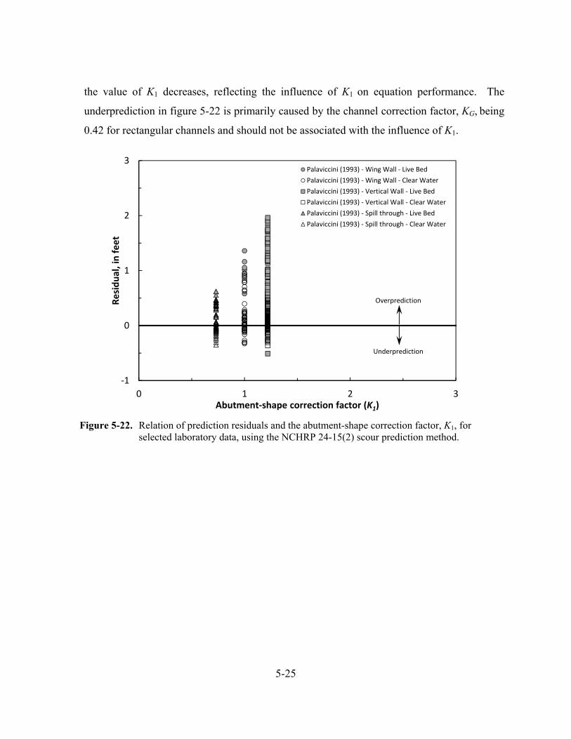
5-25
the value of K1 decreases, reflecting the influence of K1 on equation performance. The
underprediction in figure 5-22 is primarily caused by the channel correction factor, KG, being
0.42 for rectangular channels and should not be associated with the influence of K1.
Figure 5-22. Relation of prediction residuals and the abutment-shape correction factor, K1, for selected laboratory data, using the NCHRP 24-15(2) scour prediction method.
‐1
0
1
2
3
0 1 2 3
Residual, in feet
Abutment‐shape correction factor (K1)
Palaviccini (1993) ‐ Wing Wall ‐ Live Bed
Palaviccini (1993) ‐ Wing Wall ‐ Clear Water
Palaviccini (1993) ‐ Vertical Wall ‐ Live Bed
Palaviccini (1993) ‐ Vertical Wall ‐ Clear Water
Palaviccini (1993) ‐ Spill through ‐ Live Bed
Palaviccini (1993) ‐ Spill through ‐ Clear Water
Overprediction
Underprediction
5-26
Abutment-skew correction factor (K2)
Only two abutment-scour measurements in the laboratory data were associated with a skewed
abutment, and therefore, a plot of the residuals associated with K2 was of minimal benefit and
not included in the report. However, a brief review of the K2 correction factor follows. Based
on the work of earlier investigations, such as Froehlich (1989) and Melville (1992), it
generally has been accepted that skewed abutments pointing downstream produce smaller
scour depths, while skewed abutments pointing upstream produce larger scour depths. Based
on this previous work, the magnitude of the decrease or increase in scour depth is about 5
percent for moderate skews and about 10 percent for severe skews. The findings of the
Briaud et al. (2009) investigation are somewhat contrary to these previous studies, with scour
depth decreasing by as much as 15 percent regardless of the abutment orientation to flow.
Based on this finding, the NCHRP 24-15(2) prediction method specifies that K2 be set to a
value of 0.85 for a skew angle of 30 degrees or greater from perpendicular, regardless of
orientation to flow, with K2 transitioning to a value of 1 as the abutment-skew angle
approaches 0. Dongol (1993) notes that laboratory investigations by Kwan (1984) and
Kandasamy (1985) found similar qualitative trends to those of Briaud et al. (2009), with
reduced scour at skewed abutments regardless of orientation to flow, providing support for
the general patterns in the Briaud et al. (2009) investigation. However, only two of the
Briaud et al. (2009) data points are associated with skewed abutments, one pointing
downstream and the other upstream. Because of the limited number of data, the relation for
determining K2 should be used with caution, and further investigation of the influence of
skew on abutment-scour depth could be beneficial to confirm the equation for determining
K2.
5-27
Channel-geometry correction factor (KG)
Briaud et al. (2009) concluded that channel geometry influences abutment-scour depth, with
rectangular channels reducing scour by approximately 60 percent in comparison to
compound channels. To account for this influence, a channel-geometry correction factor, KG,
was included in the NCHRP 24-15(2) scour prediction method, with KG having a value of 1.0
for compound channels and 0.42 for rectangular channels. The relation of the prediction
residuals for selected laboratory data with respect to KG is shown in figures 5-23A through C.
These data include the clear-water scour conditions for vertical-wall, wing-wall, and spill-
through abutments for selected data, with values of K2 and KL equal to 1.0. The upper bound
of the prediction residuals for the rectangular-channel data is smaller than that of the
compound-channel data. The magnitude of this difference varies with abutment shape with
the vertical- and wing-wall abutments having a larger difference than that of the spill-through
abutments. The frequency and magnitude of underprediction is much larger for the
rectangular-channel data than for the compound-channel data. To provide perspective on the
influence of KG, figure 5-24 shows the same data as in figure 5-23C, with the KG value for
the rectangular-channel data arbitrarily set to 1.0. This value of KG for the rectangular-
channel data removes most of the underpredictions. A review of figures 5-23A–C highlights
how the NCHRP 24-15(2) method will yield frequent underpredictions for clear-water scour
sites with rectangular channels. This is the pattern previously noted in figures 5-1 through 5-
6, with most of the underprediction in those figures associated with clear-water scour
conditions in rectangular channels. As noted later in the report, this pattern is of concern for
the field data where floodplain relief bridges and bridges crossing swamps with poorly
defined channels are classified as rectangular channels under clear-water scour conditions
and also have frequent and, at times, large underprediction.
Figure 5-25 presents the relation from Briaud et al. (2009) that was used to analyze the
influence of channel geometry on abutment-scour depth and, in turn, develop the KG
correction factor. As can be seen, a relation indicates that rectangular channels in the Briaud
et al. (2009) data have smaller scour depths than compound channels. (Note: Only two of the
three compound-channel data points, the largest of the relative scour values, are shown in
5-28
figure 5-25. The other 5 data points are associated with rectangular channels, and only the 2
data points that form the lower envelope of the rectangular-channel data are shown as
circular symbols.) Because of the complex nature of scour, it is often difficult to isolate the
influence of a single variable, and this is likely the case with regard to the influence of
channel geometry. A review of the data in figure 5-25 indicates that hydraulic conditions
are likely contributing to this pattern rather than just the channel geometry, and this is
discussed below.
Figure 5-26 shows the relation of relative-scour depth to the total flow using the same data in
figure 5-25 along with the one additional compound-channel data point. (Note: All of the
rectangular- and compound-channel data are identified with distinct symbols in figure 5-26.)
The flow for all of the rectangular-channel data is approximately 15 cubic feet per second
(ft3/s), whereas the three compound-channel data points have flows ranging from about 15 to
27 ft3/s. The compound-channel data with a flow of about 15 ft3/s are comparable to the flow
rate of the rectangular channels, and also have a relative-scour depth comparable to the
rectangular channels. In contrast, the two compound-channel data with larger flows have
larger relative-scour depths, indicating that the differing scour patterns between the
compound and rectangular channels likely are a function of flow rather than channel
geometry. While additional research on the influence of channel geometry is warranted, the
relations in figure 5-25 indicate that it may be appropriate to use a value of 1.0 for KG at
rectangular channels. This is further supported by the work of Melville (1992) and Melville
and Coleman (2000). While these studies acknowledge the influence of channel geometry
on scour depth, they indicate that rectangular channels produce the largest scour depth,
contrary to the findings of the Briaud et al. (2009) study. Based on the work of Melville
(1992) and Melville and Coleman (2000), it would seem appropriate to use a value of 1.0 for
KG at rectangular channels rather than a value of 0.42.
To provide understanding of how a change in KG for rectangular channels will affect
equation performance, figure 5-27 shows the same data as shown in figure 5-1A with KG for
rectangular channels set to 1.0. In this situation, underprediction for clear-water scour data at
rectangular channels is largely removed. As noted later in the report, this is an important
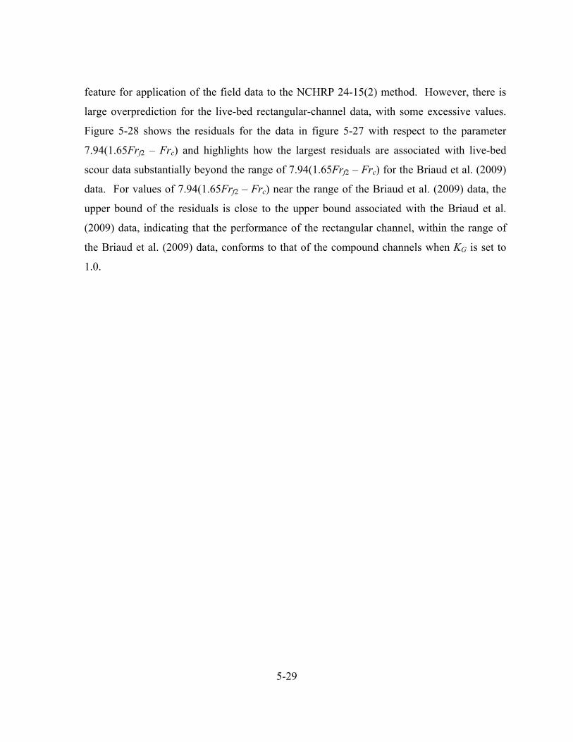
5-29
feature for application of the field data to the NCHRP 24-15(2) method. However, there is
large overprediction for the live-bed rectangular-channel data, with some excessive values.
Figure 5-28 shows the residuals for the data in figure 5-27 with respect to the parameter
7.94(1.65Frf2 – Frc) and highlights how the largest residuals are associated with live-bed
scour data substantially beyond the range of 7.94(1.65Frf2 – Frc) for the Briaud et al. (2009)
data. For values of 7.94(1.65Frf2 – Frc) near the range of the Briaud et al. (2009) data, the
upper bound of the residuals is close to the upper bound associated with the Briaud et al.
(2009) data, indicating that the performance of the rectangular channel, within the range of
the Briaud et al. (2009) data, conforms to that of the compound channels when KG is set to
1.0.
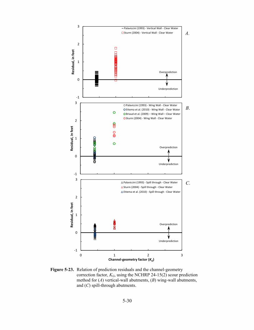
5-30
A.
B.
C.
‐1
0
1
2
3
0 1 2 3
Residual, in feet
Channel geometry factor (KG)
Palaviccini (1993) ‐ Vertical Wall ‐ Clear Water
Sturm (2004) ‐ Vertical Wall ‐ Clear Water
Overprediction
Underprediction
‐1
0
1
2
3
0 1 2 3
Residual, in feet
Channel geometry factor (KG)
Palaviccini (1993) ‐ Wing Wall ‐ Clear Water
Ettema et al. (2010) ‐ Wing Wall ‐ Clear Water
Briaud et al. (2009) – Wing Wall – Clear Water
Sturm (2004) ‐ Wing Wall ‐ Clear Water
Overprediction
Underprediction
‐1
0
1
2
3
0 1 2 3
Residual, in feet
Channel‐geometry factor (KG)
Palaviccini (1993) ‐ Spill through ‐ Clear Water
Sturm (2004) ‐ Spill through ‐ Clear Water
Ettema et al. (2010) ‐ Spill through ‐ Clear Water
Overprediction
Underprediction
Figure 5-23. Relation of prediction residuals and the channel-geometry correction factor, KG, using the NCHRP 24-15(2) scour prediction method for (A) vertical-wall abutments, (B) wing-wall abutments, and (C) spill-through abutments.
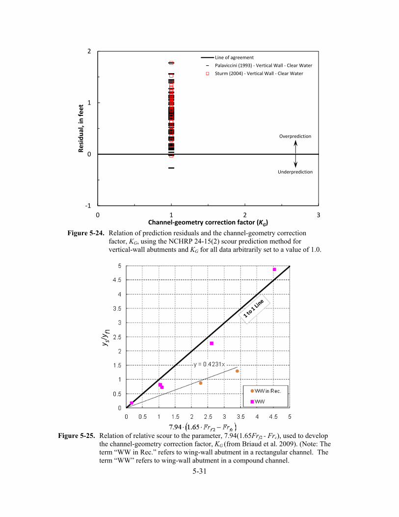
5-31
Figure 5-24. Relation of prediction residuals and the channel-geometry correction factor, KG, using the NCHRP 24-15(2) scour prediction method for vertical-wall abutments and KG for all data arbitrarily set to a value of 1.0.
Figure 5-25. Relation of relative scour to the parameter, 7.94(1.65Frf2 - Frc), used to develop the channel-geometry correction factor, KG (from Briaud et al. 2009). (Note: The term “WW in Rec.” refers to wing-wall abutment in a rectangular channel. The term “WW” refers to wing-wall abutment in a compound channel.
‐1
0
1
2
0 1 2 3
Residual, in feet
Channel‐geometry correction factor (KG)
Line of agreement
Palaviccini (1993) ‐ Vertical Wall ‐ Clear Water
Sturm (2004) ‐ Vertical Wall ‐ Clear Water
Overprediction
Underprediction
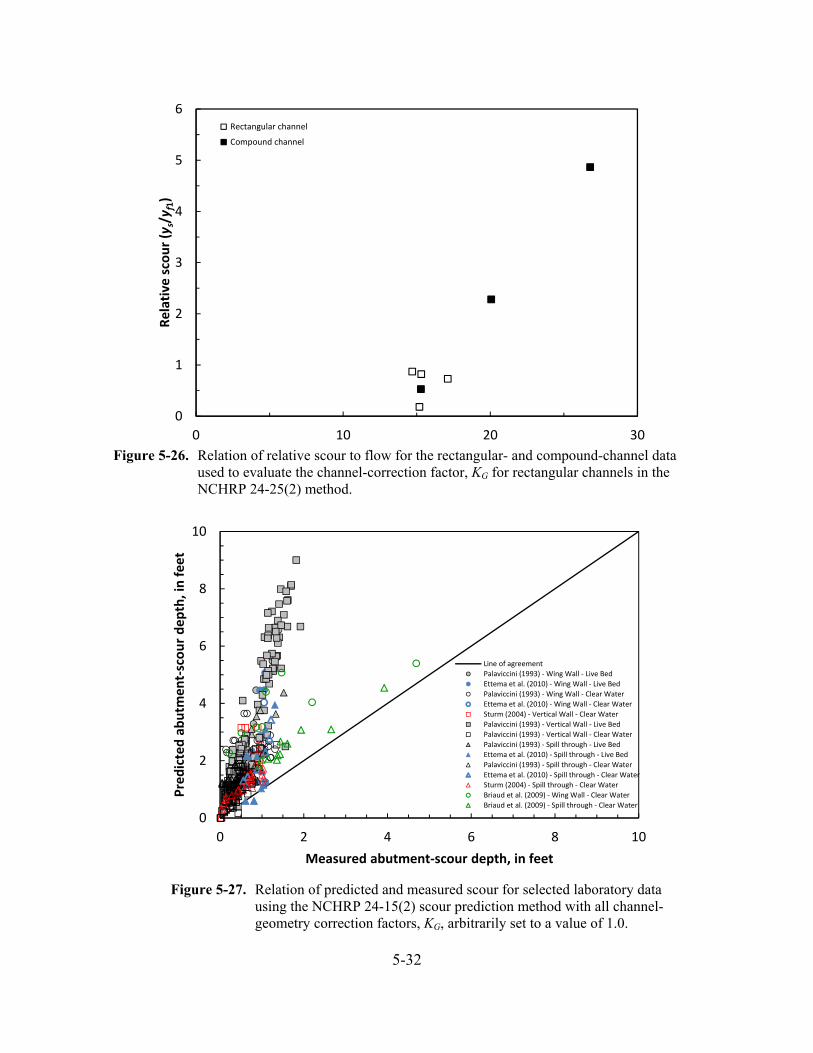
5-32
0
2
4
6
8
10
0 2 4 6 8 10
Predicted abutm
ent‐scour depth, in feet
Measured abutment‐scour depth, in feet
Line of agreement
Palaviccini (1993) ‐ Wing Wall ‐ Live Bed
Ettema et al. (2010) ‐ Wing Wall ‐ Live Bed
Palaviccini (1993) ‐ Wing Wall ‐ Clear Water
Ettema et al. (2010) ‐ Wing Wall ‐ Clear Water
Sturm (2004) ‐ Vertical Wall ‐ Clear Water
Palaviccini (1993) ‐ Vertical Wall ‐ Live Bed
Palaviccini (1993) ‐ Vertical Wall ‐ Clear Water
Palaviccini (1993) ‐ Spill through ‐ Live Bed
Ettema et al. (2010) ‐ Spill through ‐ Live Bed
Palaviccini (1993) ‐ Spill through ‐ Clear Water
Ettema et al. (2010) ‐ Spill through ‐ Clear Water
Sturm (2004) ‐ Spill through ‐ Clear Water
Briaud et al. (2009) ‐ Wing Wall ‐ Clear Water
Briaud et al. (2009) ‐ Spill through ‐ Clear Water
0
1
2
3
4
5
6
0 10 20 30
Relative scour (y
s/y f
1)
Flow, in cubic feet per second
Rectangular channel
Compound channel
Figure 5-26. Relation of relative scour to flow for the rectangular- and compound-channel data used to evaluate the channel-correction factor, KG for rectangular channels in the NCHRP 24-25(2) method.
Figure 5-27. Relation of predicted and measured scour for selected laboratory data using the NCHRP 24-15(2) scour prediction method with all channel-geometry correction factors, KG, arbitrarily set to a value of 1.0.
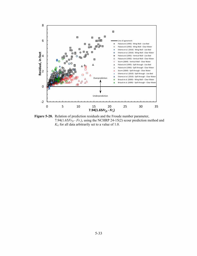
5-33
Figure 5-28. Relation of prediction residuals and the Froude number parameter, 7.94(1.65Frf2 - Frc), using the NCHRP 24-15(2) scour prediction method and KG for all data arbitrarily set to a value of 1.0.
‐2
0
2
4
6
8
0 5 10 15 20 25 30 35
Residual, in feet
7.94(1.65Frf2 ‐ Frc)
Line of agreement
Palaviccini (1993) ‐ Wing Wall ‐ Live Bed
Palaviccini (1993) ‐ Wing Wall ‐ Clear Water
Ettema et al. (2010) ‐ Wing Wall ‐ Live Bed
Ettema et al. (2010) ‐ Wing Wall ‐ Clear Water
Palaviccini (1993) ‐ Vertical Wall ‐ Live Bed
Palaviccini (1993) ‐ Vertical Wall ‐ Clear Water
Sturm (2004) ‐ Vertical Wall ‐ Clear Water
Palaviccini (1993) ‐ Spill through ‐ Live Bed
Palaviccini (1993) ‐ Spill through ‐ Clear Water
Sturm (2004) ‐ Spill through ‐ Clear Water
Ettema et al. (2010) ‐ Spill through ‐ Live Bed
Ettema et al. (2010) ‐ Spill through ‐ Clear Water
Briaud et al. (2009) – Wing Wall – Clear Water
Briaud et al. (2009) – Spill through – Clear Water
Overprediction
Underprediction
5-34
Abutment-location correction factor (KL)
The NCHRP 24-15(2) scour prediction method includes a correction factor for abutment
location (KL) with respect to the main channel. The maximum value for KL is 1.35 and
occurs when the abutment is located at the channel bank or protrudes into the main channel.
The value of KL transitions to 1.0 when the abutment toe is a distance of 1.5yf1 from the
channel bank. As noted previously, the largest overpredictions in figure 5-1 in the Sturm
(2004) and Ettema et al. (2010) data are associated with abutments located at the bank or
protruding into the main channel. The relation of the prediction residuals with respect to KL
for vertical-wall and spill-through abutment data from Sturm (2004) is shown in figures 5-
29A and B, respectively, and demonstrates the larger overprediction associated with bankline
and protruding abutments.
Rather than using a correction factor for abutment location to account for scour associated
with bankline and protruding abutments, an alternate method is to use the hydraulic
characteristics associated with the channel rather than the floodplain. The standard method
for applying the NCHRP 24-15(2) method (chapter 4) uses a combination of floodplain and
channel hydraulics for bankline and protruding abutments. For protruding abutments, the
flow depth and velocity used in equation 4-1 are associated with the main channel.
Therefore, at such abutments it may be redundant to adjust the predicted scour depth for
abutment location with a KL value of 1.35. For bankline abutments, the flow depth and
velocity reflect values associated with the floodplain and the main channel, respectively. For
such abutments, it may be appropriate to use the flow depth in the main channel rather than
the flow depth in the floodplain to account for the increased potential for scour, thereby
removing the need to adjust the predicted scour depth for abutment location with a KL value
of 1.35. Figures 5-30A and B show the relation of measured abutment-scour depth to
predicted scour for the laboratory data with bankline or protruding abutments, with figure 5-
30A reflecting computations by using the standard method for applying the NCHRP 24-15(2)
method with a KL value of 1.35, and figure 5-30B reflecting computations by using the
channel hydraulics with a KL value of 1.0. In the case of the one point in the Briaud et al.
(2009) data, using the channel hydraulics with a KL value of 1.0 produces a minor
5-35
underprediction, indicating that the modified approach using the channel hydraulics may be
appropriate. In the case of the Ettema et al. (2010) data, the magnitude of the overpredictions
is decreased, with a small increase in the frequency and magnitude of underprediction. In the
case of the Sturm (2004) data, the magnitude of the overpredictions increases for all of the
data. This increased magnitude in overprediction can be attributed to the channel flow
depths in the Sturm (2004) data being 6 to 8 times that of the floodplain flow depths. In
contrast, the channel flow depths for the Ettema et al. (2010) and Briaud et al. (2009) data are
approximately 2 times the floodplain flow depths. The prediction patterns in figures 5-30A
and B indicate that using the channel hydraulics with a KL value of 1.0 is reasonable where
ratios of channel to floodplain flow depths are approximately 2, but can become excessive as
that ratio increases. Because the number of data in figure 5-30 is relatively small, additional
research of this matter would be advisable.
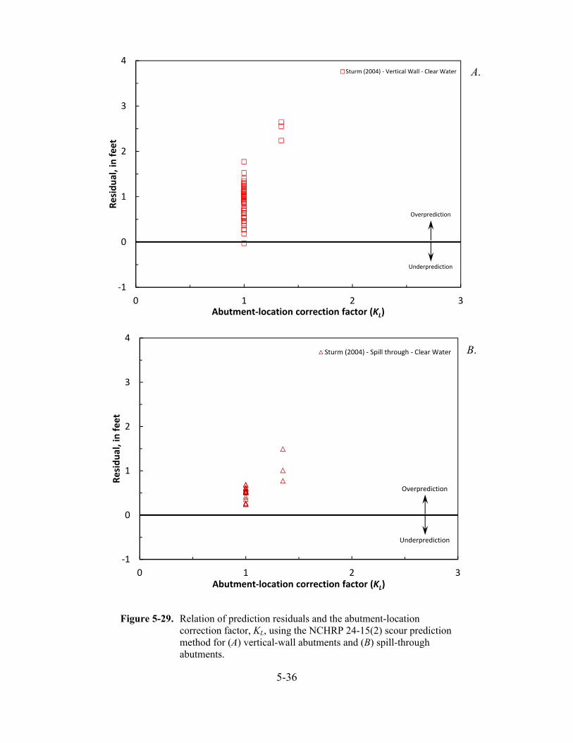
5-36
Figure 5-29. Relation of prediction residuals and the abutment-location correction factor, KL, using the NCHRP 24-15(2) scour prediction method for (A) vertical-wall abutments and (B) spill-through abutments.
‐1
0
1
2
3
4
0 1 2 3
Residual, in feet
Abutment‐location correction factor (KL)
Sturm (2004) ‐ Vertical Wall ‐ Clear Water
Overprediction
Underprediction
‐1
0
1
2
3
4
0 1 2 3
Residual, in feet
Abutment‐location correction factor (KL)
Sturm (2004) ‐ Spill through ‐ Clear Water
Overprediction
Underprediction
A.
B.
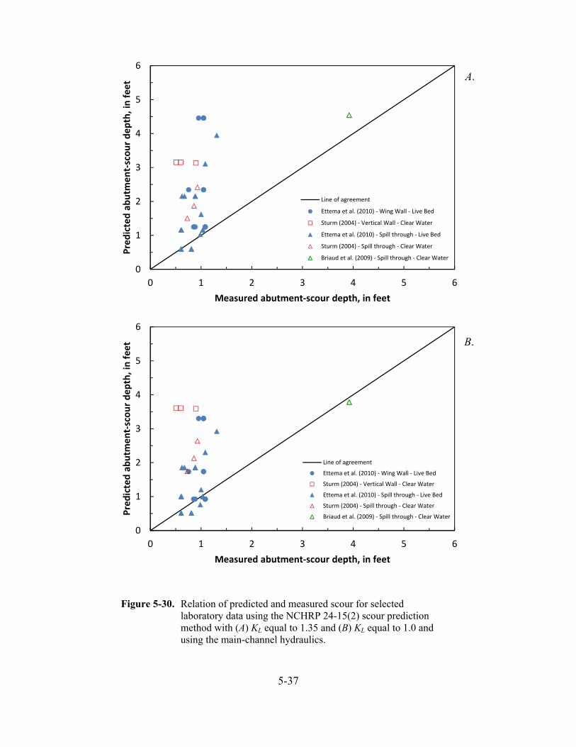
5-37
Figure 5-30. Relation of predicted and measured scour for selected laboratory data using the NCHRP 24-15(2) scour prediction method with (A) KL equal to 1.35 and (B) KL equal to 1.0 and using the main-channel hydraulics.
0
1
2
3
4
5
6
0 1 2 3 4 5 6
Predicted abutm
ent‐scour depth, in feet
Measured abutment‐scour depth, in feet
Line of agreement
Ettema et al. (2010) ‐ Wing Wall ‐ Live Bed
Sturm (2004) ‐ Vertical Wall ‐ Clear Water
Ettema et al. (2010) ‐ Spill through ‐ Live Bed
Sturm (2004) ‐ Spill through ‐ Clear Water
Briaud et al. (2009) ‐ Spill through ‐ Clear Water
0
1
2
3
4
5
6
0 1 2 3 4 5 6
Predicted abutm
ent‐scour depth, in feet
Measured abutment‐scour depth, in feet
Line of agreement
Ettema et al. (2010) ‐ Wing Wall ‐ Live Bed
Sturm (2004) ‐ Vertical Wall ‐ Clear Water
Ettema et al. (2010) ‐ Spill through ‐ Live Bed
Sturm (2004) ‐ Spill through ‐ Clear Water
Briaud et al. (2009) ‐ Spill through ‐ Clear Water
A.
B.
5-38
Pressure-flow correction factor (Kp)
No laboratory data were associated with pressure flow; therefore, no assessment was made of
this correction factor. However, a brief review of the Kp correction factor follows. The Kp
correction factor for the NCHRP 24-15(2) method was developed from numerical model
simulations. The value of Kp is 1 just at the onset of pressure flow when the water surface
comes in contact with the low chord of the bridge. As the water surface moves above the
low chord, the value of Kp increases, reaching a maximum value of 1.92 when the water
surface reaches the top of the bridge deck. The value of Kp diminishes as the water surface
moves above the bridge deck and becomes 1 when the ratio of the water depth above the low
chord to that of the bridge-deck thickness reaches a value of 3.0. For pressure-flow
conditions, Briaud et al. (2009) recommend using the flow depth from the channel bottom to
the low chord rather than the free-surface flow depth, and acknowledge that Kp will be
conservative. The Kp correction factor can be as large as 1.92, which will substantially
increase the predicted scour depth. There are 46 bridges in the field data with pressure-flow
conditions, and values of Kp at these sites range from 1.1 to 1.92, with a median value of
1.56.
5-39
5.3 Analysis of the USGS Field Data
The NCHRP 24-15(2) method was evaluated with the field measurements of abutment scour
listed in table 1-1. The analysis included a comparison of predicted and measured scour, an
evaluation of the relative influence of selected variables in the NCHRP 24-15(2) equation
(equation 4-1) on predicted scour, an evaluation of prediction residuals with respect to selected
equation variables, and alternate methods to possibly improve the performance of the NCHRP
24-15(2) method. The analysis is presented in the following report sections.
5.3.1 Relation of Measured and Predicted Scour
Figure 5-31 shows the relation of measured abutment-scour depth to predicted scour for the
application of the NCHRP 24-15(2) method to the USGS field data listed in table 1-1. The
application method is described in chapter 4 of this report. The field data in this figure are
grouped as presented in table 1-1, with the exception that a subset of 41 South Carolina
measurements associated with floodplain relief bridges and swampy sites with poorly defined
channels were plotted as an additional group. Most of the data in this subset are located in the
Coastal Plain of South Carolina, with the exception of two data points located in the Piedmont.
(Refer to report section 3.3 for additional information regarding this subset of data.) As with the
analysis of the NCHRP 24-20 method, sites listed in table 3-1 are identified in figure 5-31 using
the associated site number. The site characteristics associated with sites 7 through 9 (table 3-1)
are inconsequential in the analysis of NCHRP 24-15(2) and were not identified. Other graphs in
this analysis will identify the sites listed in table 3-1 in a similar manner. To better visualize the
trends in figure 5-31, the data points associated with each data group are shown in figure 5-32 as
a series of plots. All of the field data are shown as hollow circles, with the selected data groups
identified with solid circles. The lower gradient and wide floodplain streams associated with the
South Carolina Relief/Swamp Bridge data and the Coastal Plain data are shown in figures 5-32A
and B, respectively. The frequent underprediction in these data can be attributed, in part, to
lower Froude numbers and frequent rectangular channels having a KG correction factor of 0.42.
A similar pattern of underprediction associated with these characteristics was noted in the
analysis of the laboratory data and is described in more detail in the analysis of the residuals.
5-40
For the cohesive sediments of the South Carolina Piedmont (figure 5-32C), underprediction is
infrequent, and the magnitude of the underprediction is not frequently excessive. The NCHRP
24-15(2) method was developed for cohesive soils and the reasonable performance with the
South Carolina Piedmont data indicates it is applicable to such sediments. The largest
overprediction for the Piedmont data (approximately 25 ft) is associated with pressure flow
having a Kp correction factor of 1.68. The next three largest overpredictions (approximately 15
ft or greater) are associated with larger Froude numbers which, in the laboratory analysis, tended
to have a larger frequency and magnitude of overprediction. The Maine data (figure 5-32D)
have the most excessive overprediction for the field data. This excessive overprediction can be
attributed, in part, to larger Froude numbers, more frequent occurrence of pressure flow with Kp
correction factors greater than 1.0, and protruding abutments for all of the data with abutment-
location correction factors, KL, of 1.35. If the value of KL is set to 1.0 for the Maine data, the
excessive overprediction is substantially improved. The few underpredictions in figure 5-32D
are associated with smaller Froude numbers, which tend to produce more frequent
underpredictions. For the cohesive sediments of the Alabama data (figure 5-32E), there is
frequent underprediction. All of the Alabama data are associated with rectangular channels, and
the underprediction can be attributed, in part, to the lower KG correction factor of 0.42 for such
channels. If the value of KG was set to 1.0 for the Alabama data, the performance of the data
would be similar to that of the South Carolina Piedmont data with minimal underprediction. The
NBSD data are shown in figure 5-32F. Most of these data, including the 2 largest
overpredictions, are associated with protruding abutments with KL correction factors of 1.35. As
with the Maine data, if the value of KL is set to 1.0 for the NBSD data, the magnitude of the
overprediction is reduced with minimal underprediction.
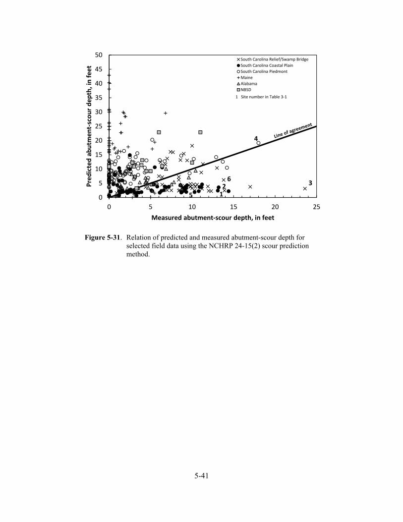
5-41
Figure 5-31. Relation of predicted and measured abutment-scour depth for selected field data using the NCHRP 24-15(2) scour prediction method.
36
152
4
0
5
10
15
20
25
30
35
40
45
50
0 5 10 15 20 25
Predicted abutm
ent‐scour depth, in feet
Measured abutment‐scour depth, in feet
South Carolina Relief/Swamp Bridge
South Carolina Coastal Plain
South Carolina Piedmont
Maine
Alabama
NBSD
1 Site number in Table 3‐1
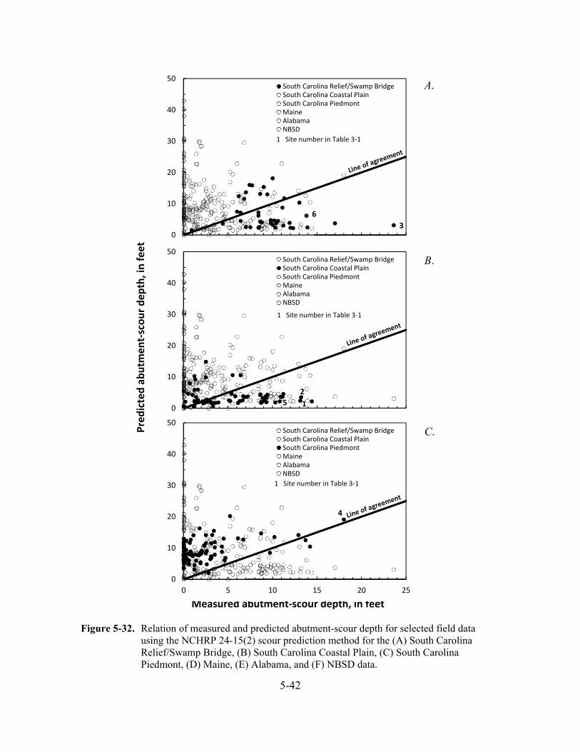
5-42
Figure 5-32. Relation of measured and predicted abutment-scour depth for selected field data using the NCHRP 24-15(2) scour prediction method for the (A) South Carolina Relief/Swamp Bridge, (B) South Carolina Coastal Plain, (C) South Carolina Piedmont, (D) Maine, (E) Alabama, and (F) NBSD data.
Predicted abutm
ent‐scour depth, in feet
Measured abutment‐scour depth, in feet
A.
B.
C.
3
6
0
10
20
30
40
50
0 5 10 15 20 25
South Carolina Relief/Swamp BridgeSouth Carolina Coastal PlainSouth Carolina PiedmontMaineAlabamaNBSD
1 Site number in Table 3‐1
15
2
0
10
20
30
40
50
0 5 10 15 20 25
South Carolina Relief/Swamp BridgeSouth Carolina Coastal PlainSouth Carolina PiedmontMaineAlabamaNBSD
1 Site number in Table 3‐1
4
0
10
20
30
40
50
0 5 10 15 20 25
South Carolina Relief/Swamp BridgeSouth Carolina Coastal PlainSouth Carolina PiedmontMaineAlabamaNBSD
1 Site number in Table 3‐1

5-43
Figure 5-32. - Continued. Relation of measured and predicted abutment-scour depth for
selected field data using the NCHRP 24-15(2) scour prediction method for the (A) South Carolina Relief/Swamp Bridges, (B) South Carolina Coastal Plain, (C) South Carolina Piedmont, (D) Maine, (E) Alabama, and (F) NBSD data.
Predicted abutm
ent‐scour depth, in feet
Measured abutment‐scour depth, in feet
D.
E.
F.
0
10
20
30
40
50
0 5 10 15 20 25
South Carolina Relief/Swamp BridgeSouth Carolina Coastal PlainSouth Carolina PiedmontMaineAlabamaNBSD
0
10
20
30
40
50
0 5 10 15 20 25
South Carolina Relief/Swamp BridgeSouth Carolina Coastal PlainSouth Carolina PiedmontMaineAlabamaNBSD
0
10
20
30
40
50
0 5 10 15 20 25
South Carolina Relief/Swamp BridgeSouth Carolina Coastal PlainSouth Carolina PiedmontMaineAlabamaNBSD
5-44
5.3.2 Influence of Selected Explanatory Variables on Predicted Scour
To provide some perspective on the influence of each explanatory variable in equation 4-1 on
predicted scour for the field data, the following series of figures (figures 5-33 through 5-39)
show the relation of predicted to measured scour as each explanatory variable is progressively
added to the equation. (This series of plots is shown for the laboratory data in report section
5.2.2.) The progression of adding the explanatory variables is as follows: 7.94(1.65Frf2 – Frc),
KRe, K1, K2, KG, KL, and Kp. Some notable features regarding this series of figures are as follows:
The prediction pattern in figure 5-33 essentially shows no underprediction, but large
overprediction that at times is excessive. While overprediction can be excessive, the
prediction patterns indicate that the core explanatory variable, 7.94(1.65Frf2 – Frc), is
capturing, in some measure, the trends of the field data, with predicted scour increasing
as measured scour increases. The largest overpredictions in the Maine data are associated
with large values of Frf2 and small values of Frc, which yield large estimates of scour
when applied to 7.94(1.65Frf2 – Frc). It is notable that the non-cohesive sediments of the
South Carolina Coastal Plain and the Relief/Swamp Bridges perform best and that the
Pee Dee River at I-95, with the largest measured scour depth, is not underpredicted. In
contrast, the cohesive sediments of the South Carolina Piedmont tend to have higher
estimates of scour.
The progression from figure 5-33 to 5-34 highlights how the Reynolds number
parameter, KRe, substantially reduces the magnitude of predicted scour, producing
underprediction in the lower gradient streams of the Coastal Plain and Relief/Swamp
Bridges. (Note: The vertical scales on figures 5-33 and 5-34 are different to accommodate
the differing data ranges.) The range for KRe for the field data is from 0.3 to 0.98, with an
average value of 0.49, indicating that KRe will tend to decrease predicted scour by about
50 percent on average. This trend is in contrast to the laboratory data where the range of
KRe is larger and increases predicted scour by about 60 percent on average (report section
5.2.2). As noted in report section 5.2.3(iii), the range of the Reynolds number for the
field data is much larger than that of the Briaud et al. (2009) data, which produces smaller
values of KRe (figure 5-20) and thus smaller values of predicted scour.
5-45
The progression from figure 5-34 to 5-35 highlights the influence of K1 on predicted
scour, with spill-through abutments showing a decrease in the magnitude of predicted
scour and, therefore, an increase in underprediction. The increased underprediction is
most noticeable in the lower gradient streams of the Coastal Plain and Relief/Swamp
Bridges.
The progression from figure 5-35 to 5-36 highlights the influence of K2 on predicted
scour, moderately reducing predicted scour at skewed abutments.
The progression from figure 5-36 to 5-37 highlights the influence of KG on predicted
scour for rectangular channels, substantially increasing the frequency and magnitude of
underprediction for such channels. This increased underprediction is associated with the
lower gradient streams of the Coastal Plain and Relief/Swamp Bridges, as well as the
relief bridges in the Alabama data, where rectangular channels are common.
The progression from figure 5-37 to 5-38 highlights the influence of KL on predicted
scour for bankline and protruding abutments, substantially increasing the overprediction
for such abutments. The increased overprediction is largely associated with the Maine
and NBSD data and with some of the Relief/Swamp Bridges of South Carolina. (Note:
Most of the swamp bridges in South Carolina do not have main channels. However, a
few sites have small defined channels where the abutments are at the bankline or protrude
into the small channel.)
The progression from figure 5-38 to 5-39 highlights the influence of Kp on predicted
scour for pressure-flow conditions, increasing the value of predicted scour. The
increased overprediction is largely associated with the Maine and Alabama data, with
some in the NBSD and South Carolina data.
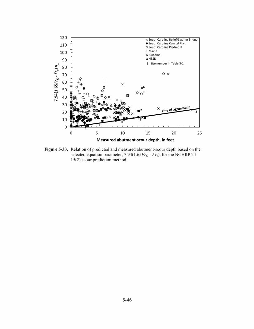
5-46
3
6
15
2
4
0
10
20
30
40
50
60
70
80
90
100
110
120
0 5 10 15 20 25
7.94(1.65Fr
f2‐Fr
c) y
1
Measured abutment‐scour depth, in feet
South Carolina Relief/Swamp BridgeSouth Carolina Coastal PlainSouth Carolina PiedmontMaineAlabamaNBSD
1 Site number in Table 3‐1
Figure 5-33. Relation of predicted and measured abutment-scour depth based on the selected equation parameter, 7.94(1.65Frf2 - Frc), for the NCHRP 24-15(2) scour prediction method.
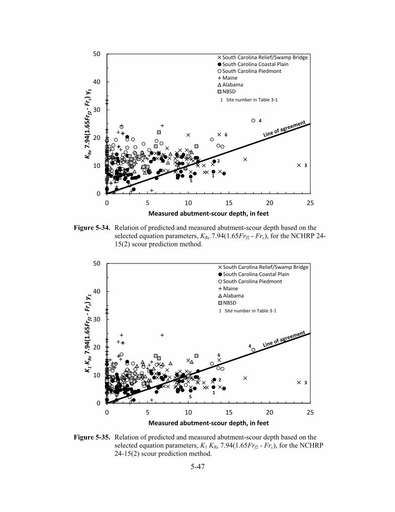
5-47
3
6
15
2
4
0
10
20
30
40
50
0 5 10 15 20 25
K1KRe7.94(1.65Fr
f2‐Fr
c) y
1
Measured abutment‐scour depth, in feet
South Carolina Relief/Swamp BridgeSouth Carolina Coastal PlainSouth Carolina PiedmontMaineAlabamaNBSD
1 Site number in Table 3‐1
Figure 5-35. Relation of predicted and measured abutment-scour depth based on the selected equation parameters, K1 KRe 7.94(1.65Frf2 - Frc), for the NCHRP 24-15(2) scour prediction method.
3
6
15
2
4
0
10
20
30
40
50
0 5 10 15 20 25
KRe7.94(1.65Fr
f2‐Fr
c) y
1
Measured abutment‐scour depth, in feet
South Carolina Relief/Swamp BridgeSouth Carolina Coastal PlainSouth Carolina PiedmontMaineAlabamaNBSD
1 Site number in Table 3‐1
Figure 5-34. Relation of predicted and measured abutment-scour depth based on the selected equation parameters, KRe 7.94(1.65Frf2 - Frc), for the NCHRP 24-15(2) scour prediction method.
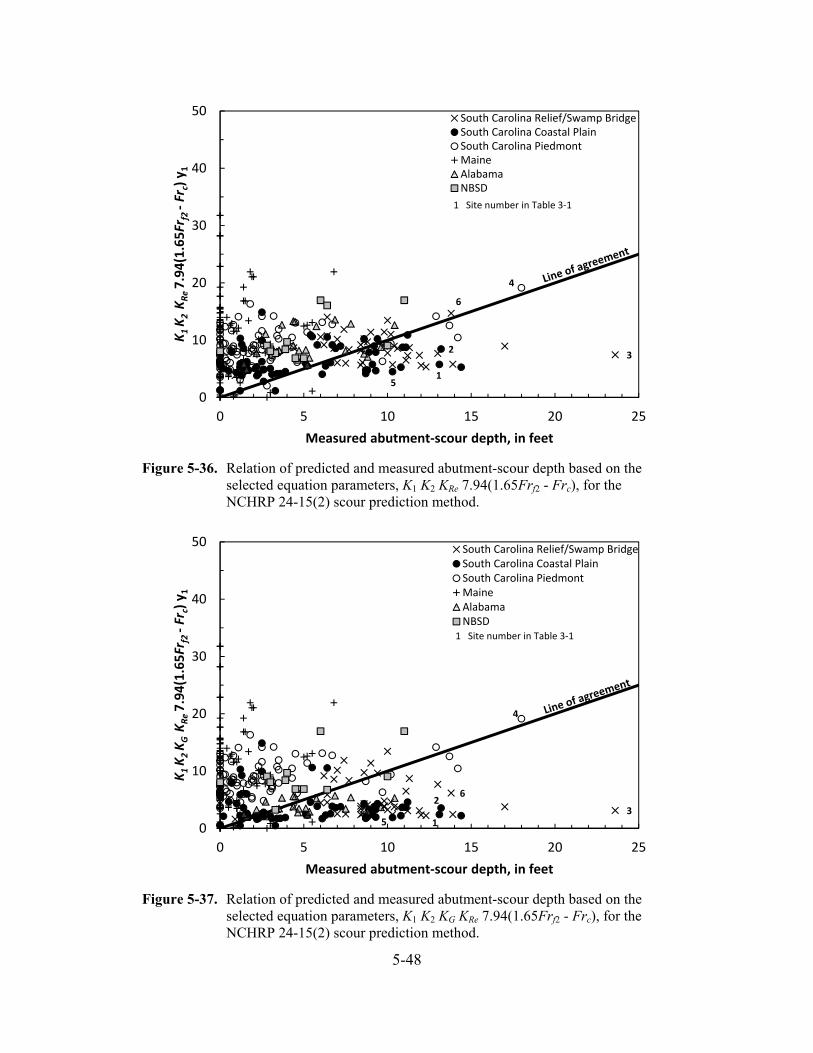
5-48
3
6
15
2
4
0
10
20
30
40
50
0 5 10 15 20 25
K1 K
2 K
G K
Re 7.94(1.65Fr
f2‐Fr
c) y
1
Measured abutment‐scour depth, in feet
South Carolina Relief/Swamp BridgeSouth Carolina Coastal PlainSouth Carolina PiedmontMaineAlabamaNBSD
1 Site number in Table 3‐1
3
6
15
2
4
0
10
20
30
40
50
0 5 10 15 20 25
K1 K
2 K
Re 7.94(1.65Fr
f2‐Fr
c) y
1
Measured abutment‐scour depth, in feet
South Carolina Relief/Swamp BridgeSouth Carolina Coastal PlainSouth Carolina PiedmontMaineAlabamaNBSD
1 Site number in Table 3‐1
Figure 5-36. Relation of predicted and measured abutment-scour depth based on the selected equation parameters, K1 K2 KRe 7.94(1.65Frf2 - Frc), for the NCHRP 24-15(2) scour prediction method.
Figure 5-37. Relation of predicted and measured abutment-scour depth based on the selected equation parameters, K1 K2 KG KRe 7.94(1.65Frf2 - Frc), for the NCHRP 24-15(2) scour prediction method.
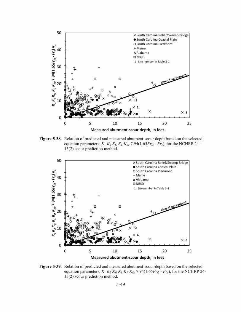
5-49
3
6
15
2
4
0
10
20
30
40
50
0 5 10 15 20 25
K1 K
2 K
G K
L K
p K
Re 7.94(1.65Fr
f2‐Fr
c) y
1
Measured abutment‐scour depth, in feet
South Carolina Relief/Swamp BridgeSouth Carolina Coastal PlainSouth Carolina PiedmontMaineAlabamaNBSD
1 Site number in Table 3‐1
3
6
15
2
4
0
10
20
30
40
50
0 5 10 15 20 25
K1 K
2 K
G K
L K
Re 7.94(1.65Fr
f2‐Fr
c) y
1
Measured abutment‐scour depth, in feet
South Carolina Relief/Swamp BridgeSouth Carolina Coastal PlainSouth Carolina PiedmontMaineAlabamaNBSD
1 Site number in Table 3‐1
Figure 5-39. Relation of predicted and measured abutment-scour depth based on the selected equation parameters, K1 K2 KG KL KP KRe 7.94(1.65Frf2 - Frc), for the NCHRP 24-15(2) scour prediction method.
Figure 5-38. Relation of predicted and measured abutment-scour depth based on the selected equation parameters, K1 K2 KG KL KRe 7.94(1.65Frf2 - Frc), for the NCHRP 24-15(2) scour prediction method.
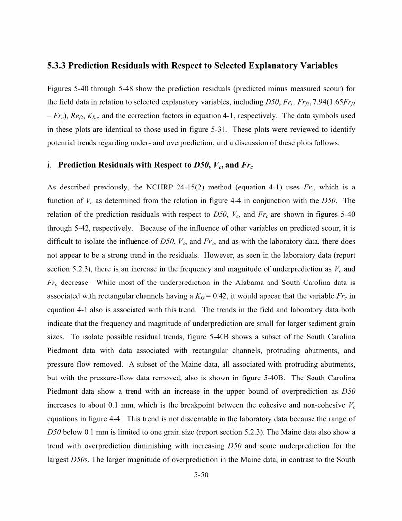
5-50
5.3.3 Prediction Residuals with Respect to Selected Explanatory Variables
Figures 5-40 through 5-48 show the prediction residuals (predicted minus measured scour) for
the field data in relation to selected explanatory variables, including D50, Frc, Frf2, 7.94(1.65Frf2
– Frc), Ref2, KRe, and the correction factors in equation 4-1, respectively. The data symbols used
in these plots are identical to those used in figure 5-31. These plots were reviewed to identify
potential trends regarding under- and overprediction, and a discussion of these plots follows.
i. Prediction Residuals with Respect to D50, Vc, and Frc
As described previously, the NCHRP 24-15(2) method (equation 4-1) uses Frc, which is a
function of Vc as determined from the relation in figure 4-4 in conjunction with the D50. The
relation of the prediction residuals with respect to D50, Vc, and Frc are shown in figures 5-40
through 5-42, respectively. Because of the influence of other variables on predicted scour, it is
difficult to isolate the influence of D50, Vc, and Frc, and as with the laboratory data, there does
not appear to be a strong trend in the residuals. However, as seen in the laboratory data (report
section 5.2.3), there is an increase in the frequency and magnitude of underprediction as Vc and
Frc decrease. While most of the underprediction in the Alabama and South Carolina data is
associated with rectangular channels having a KG = 0.42, it would appear that the variable Frc in
equation 4-1 also is associated with this trend. The trends in the field and laboratory data both
indicate that the frequency and magnitude of underprediction are small for larger sediment grain
sizes. To isolate possible residual trends, figure 5-40B shows a subset of the South Carolina
Piedmont data with data associated with rectangular channels, protruding abutments, and
pressure flow removed. A subset of the Maine data, all associated with protruding abutments,
but with the pressure-flow data removed, also is shown in figure 5-40B. The South Carolina
Piedmont data show a trend with an increase in the upper bound of overprediction as D50
increases to about 0.1 mm, which is the breakpoint between the cohesive and non-cohesive Vc
equations in figure 4-4. This trend is not discernable in the laboratory data because the range of
D50 below 0.1 mm is limited to one grain size (report section 5.2.3). The Maine data also show a
trend with overprediction diminishing with increasing D50 and some underprediction for the
largest D50s. The larger magnitude of overprediction in the Maine data, in contrast to the South
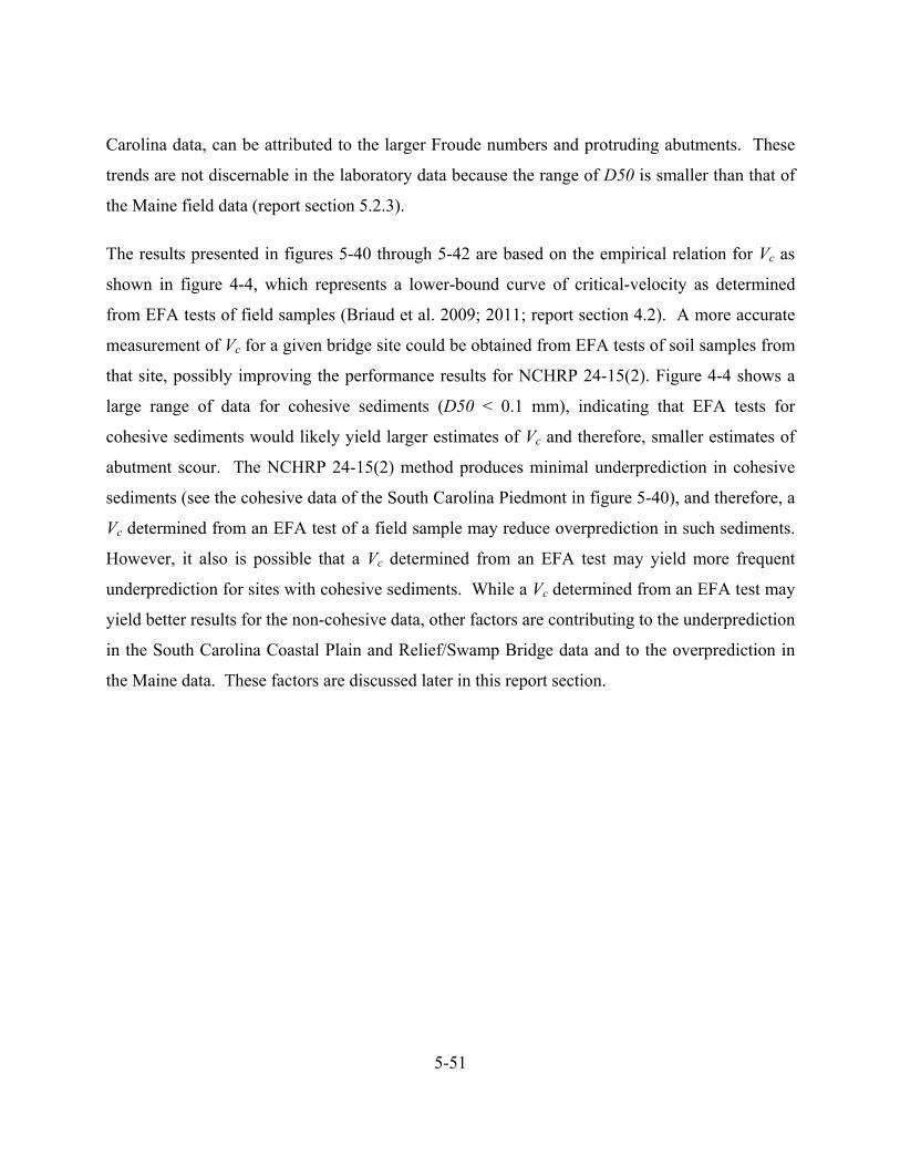
5-51
Carolina data, can be attributed to the larger Froude numbers and protruding abutments. These
trends are not discernable in the laboratory data because the range of D50 is smaller than that of
the Maine field data (report section 5.2.3).
The results presented in figures 5-40 through 5-42 are based on the empirical relation for Vc as
shown in figure 4-4, which represents a lower-bound curve of critical-velocity as determined
from EFA tests of field samples (Briaud et al. 2009; 2011; report section 4.2). A more accurate
measurement of Vc for a given bridge site could be obtained from EFA tests of soil samples from
that site, possibly improving the performance results for NCHRP 24-15(2). Figure 4-4 shows a
large range of data for cohesive sediments (D50 < 0.1 mm), indicating that EFA tests for
cohesive sediments would likely yield larger estimates of Vc and therefore, smaller estimates of
abutment scour. The NCHRP 24-15(2) method produces minimal underprediction in cohesive
sediments (see the cohesive data of the South Carolina Piedmont in figure 5-40), and therefore, a
Vc determined from an EFA test of a field sample may reduce overprediction in such sediments.
However, it also is possible that a Vc determined from an EFA test may yield more frequent
underprediction for sites with cohesive sediments. While a Vc determined from an EFA test may
yield better results for the non-cohesive data, other factors are contributing to the underprediction
in the South Carolina Coastal Plain and Relief/Swamp Bridge data and to the overprediction in
the Maine data. These factors are discussed later in this report section.
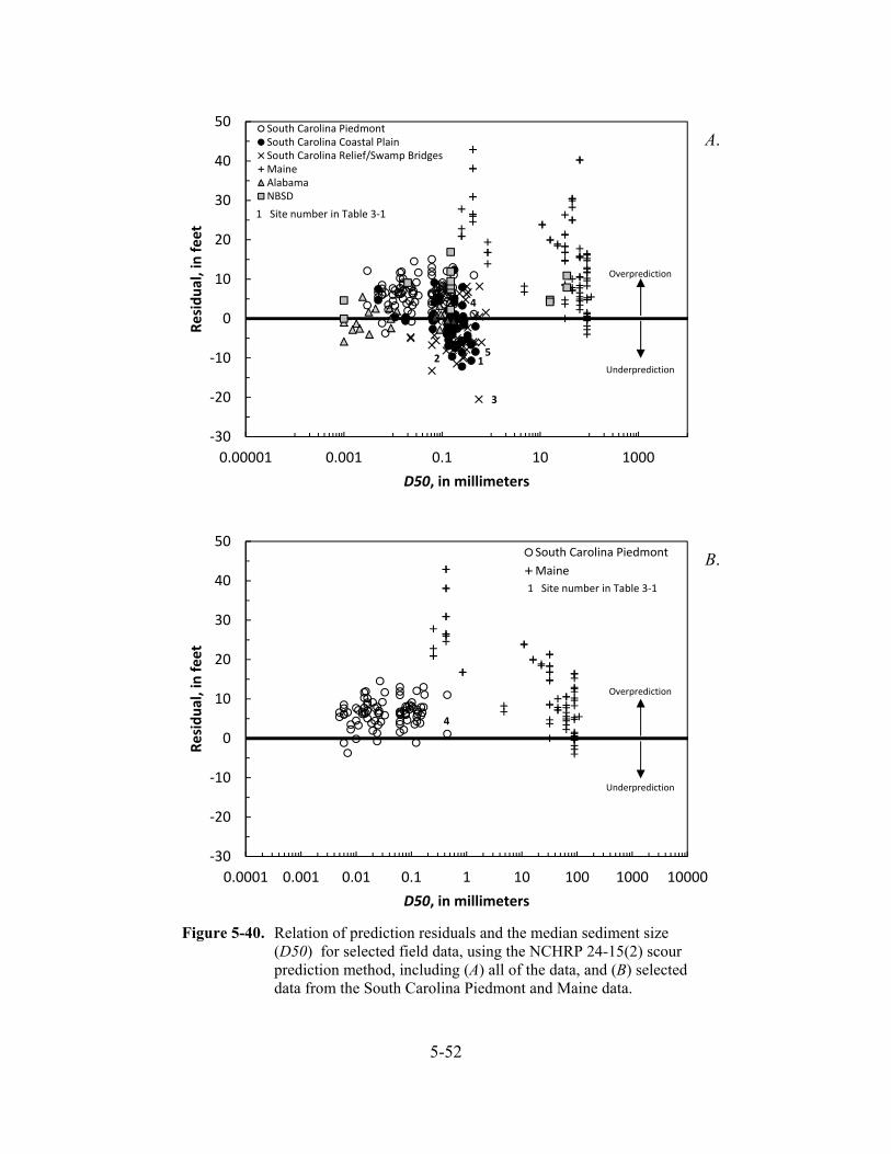
5-52
4
15
2
3
‐30
‐20
‐10
0
10
20
30
40
50
0.00001 0.001 0.1 10 1000
Residual, in feet
D50, in millimeters
South Carolina PiedmontSouth Carolina Coastal PlainSouth Carolina Relief/Swamp BridgesMaineAlabamaNBSD
Overprediction
Underprediction
1 Site number in Table 3‐1
A.
4
‐30
‐20
‐10
0
10
20
30
40
50
0.0001 0.001 0.01 0.1 1 10 100 1000 10000
Residual, in feet
D50, in millimeters
South Carolina Piedmont
Maine
Overprediction
Underprediction
1 Site number in Table 3‐1
B.
Figure 5-40. Relation of prediction residuals and the median sediment size (D50) for selected field data, using the NCHRP 24-15(2) scour prediction method, including (A) all of the data, and (B) selected data from the South Carolina Piedmont and Maine data.
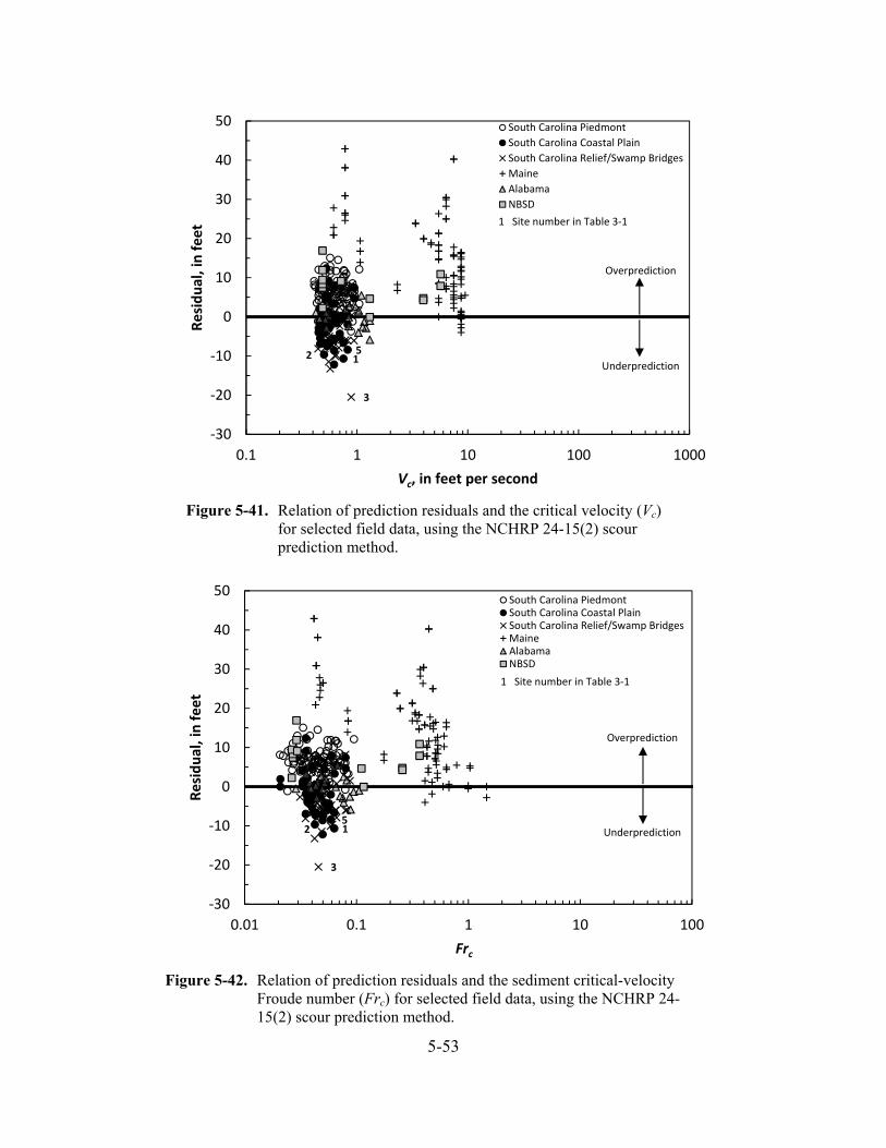
5-53
15
2
3
‐30
‐20
‐10
0
10
20
30
40
50
0.01 0.1 1 10 100
Residual, in feet
Frc
South Carolina PiedmontSouth Carolina Coastal PlainSouth Carolina Relief/Swamp BridgesMaineAlabamaNBSD
Overprediction
Underprediction
1 Site number in Table 3‐1
152
3
‐30
‐20
‐10
0
10
20
30
40
50
0.1 1 10 100 1000
Residual, in feet
Vc, in feet per second
South Carolina Piedmont
South Carolina Coastal Plain
South Carolina Relief/Swamp Bridges
Maine
Alabama
NBSD
Overprediction
Underprediction
1 Site number in Table 3‐1
Figure 5-41. Relation of prediction residuals and the critical velocity (Vc) for selected field data, using the NCHRP 24-15(2) scour prediction method.
Figure 5-42. Relation of prediction residuals and the sediment critical-velocity Froude number (Frc) for selected field data, using the NCHRP 24-15(2) scour prediction method.
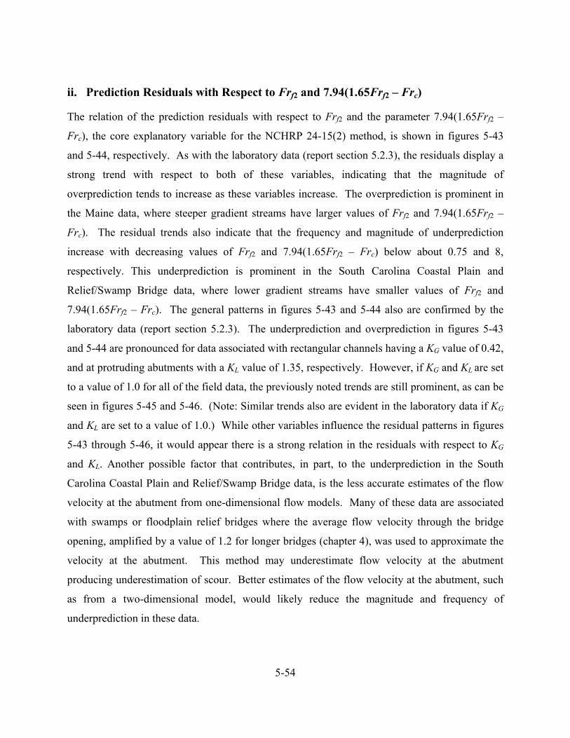
5-54
ii. Prediction Residuals with Respect to Frf2 and 7.94(1.65Frf2 – Frc)
The relation of the prediction residuals with respect to Frf2 and the parameter 7.94(1.65Frf2 –
Frc), the core explanatory variable for the NCHRP 24-15(2) method, is shown in figures 5-43
and 5-44, respectively. As with the laboratory data (report section 5.2.3), the residuals display a
strong trend with respect to both of these variables, indicating that the magnitude of
overprediction tends to increase as these variables increase. The overprediction is prominent in
the Maine data, where steeper gradient streams have larger values of Frf2 and 7.94(1.65Frf2 –
Frc). The residual trends also indicate that the frequency and magnitude of underprediction
increase with decreasing values of Frf2 and 7.94(1.65Frf2 – Frc) below about 0.75 and 8,
respectively. This underprediction is prominent in the South Carolina Coastal Plain and
Relief/Swamp Bridge data, where lower gradient streams have smaller values of Frf2 and
7.94(1.65Frf2 – Frc). The general patterns in figures 5-43 and 5-44 also are confirmed by the
laboratory data (report section 5.2.3). The underprediction and overprediction in figures 5-43
and 5-44 are pronounced for data associated with rectangular channels having a KG value of 0.42,
and at protruding abutments with a KL value of 1.35, respectively. However, if KG and KL are set
to a value of 1.0 for all of the field data, the previously noted trends are still prominent, as can be
seen in figures 5-45 and 5-46. (Note: Similar trends also are evident in the laboratory data if KG
and KL are set to a value of 1.0.) While other variables influence the residual patterns in figures
5-43 through 5-46, it would appear there is a strong relation in the residuals with respect to KG
and KL. Another possible factor that contributes, in part, to the underprediction in the South
Carolina Coastal Plain and Relief/Swamp Bridge data, is the less accurate estimates of the flow
velocity at the abutment from one-dimensional flow models. Many of these data are associated
with swamps or floodplain relief bridges where the average flow velocity through the bridge
opening, amplified by a value of 1.2 for longer bridges (chapter 4), was used to approximate the
velocity at the abutment. This method may underestimate flow velocity at the abutment
producing underestimation of scour. Better estimates of the flow velocity at the abutment, such
as from a two-dimensional model, would likely reduce the magnitude and frequency of
underprediction in these data.
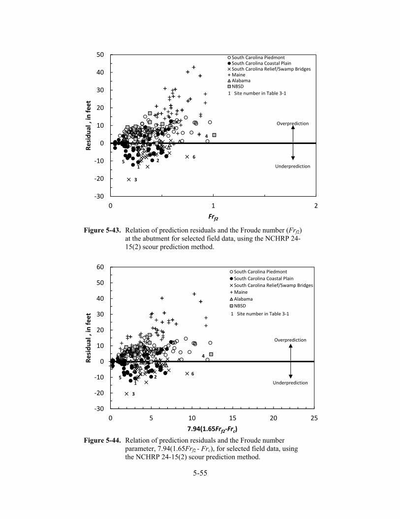
5-55
4
15 2
3
6
‐30
‐20
‐10
0
10
20
30
40
50
60
0 5 10 15 20 25
Residual , in feet
7.94(1.65Frf2‐Frc)
South Carolina Piedmont
South Carolina Coastal Plain
South Carolina Relief/Swamp Bridges
Maine
Alabama
NBSD
Overprediction
Underprediction
1 Site number in Table 3‐1
4
15 2
3
6
‐30
‐20
‐10
0
10
20
30
40
50
0 1 2
Residual , in feet
Frf2
South Carolina PiedmontSouth Carolina Coastal PlainSouth Carolina Relief/Swamp BridgesMaineAlabamaNBSD
Overprediction
Underprediction
1 Site number in Table 3‐1
Figure 5-44. Relation of prediction residuals and the Froude number parameter, 7.94(1.65Frf2 - Frc), for selected field data, using the NCHRP 24-15(2) scour prediction method.
Figure 5-43. Relation of prediction residuals and the Froude number (Frf2) at the abutment for selected field data, using the NCHRP 24-15(2) scour prediction method.
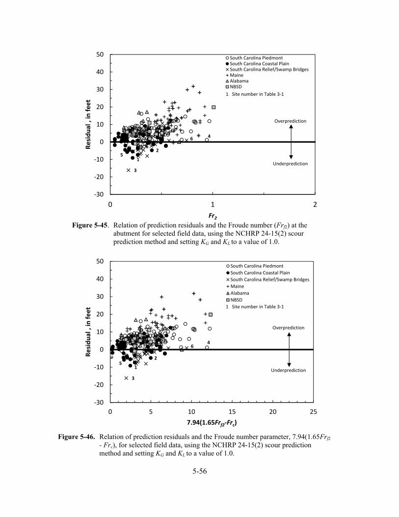
5-56
4
15
2
3
6
‐30
‐20
‐10
0
10
20
30
40
50
0 1 2
Residual , in feet
Fr2
South Carolina PiedmontSouth Carolina Coastal PlainSouth Carolina Relief/Swamp BridgesMaineAlabamaNBSD
Overprediction
Underprediction
1 Site number in Table 3‐1
4
15
2
3
6
‐30
‐20
‐10
0
10
20
30
40
50
0 5 10 15 20 25
Residual , in feet
7.94(1.65Frf2‐Frc)
South Carolina Piedmont
South Carolina Coastal Plain
South Carolina Relief/Swamp Bridges
Maine
Alabama
NBSD
Overprediction
Underprediction
1 Site number in Table 3‐1
Figure 5-45. Relation of prediction residuals and the Froude number (Frf2) at the abutment for selected field data, using the NCHRP 24-15(2) scour prediction method and setting KG and KL to a value of 1.0.
Figure 5-46. Relation of prediction residuals and the Froude number parameter, 7.94(1.65Frf2
- Frc), for selected field data, using the NCHRP 24-15(2) scour prediction method and setting KG and KL to a value of 1.0.
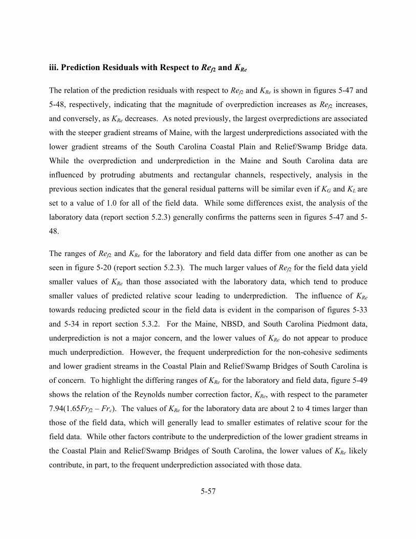
5-57
iii. Prediction Residuals with Respect to Ref2 and KRe
The relation of the prediction residuals with respect to Ref2 and KRe is shown in figures 5-47 and
5-48, respectively, indicating that the magnitude of overprediction increases as Ref2 increases,
and conversely, as KRe decreases. As noted previously, the largest overpredictions are associated
with the steeper gradient streams of Maine, with the largest underpredictions associated with the
lower gradient streams of the South Carolina Coastal Plain and Relief/Swamp Bridge data.
While the overprediction and underprediction in the Maine and South Carolina data are
influenced by protruding abutments and rectangular channels, respectively, analysis in the
previous section indicates that the general residual patterns will be similar even if KG and KL are
set to a value of 1.0 for all of the field data. While some differences exist, the analysis of the
laboratory data (report section 5.2.3) generally confirms the patterns seen in figures 5-47 and 5-
48.
The ranges of Ref2 and KRe for the laboratory and field data differ from one another as can be
seen in figure 5-20 (report section 5.2.3). The much larger values of Ref2 for the field data yield
smaller values of KRe than those associated with the laboratory data, which tend to produce
smaller values of predicted relative scour leading to underprediction. The influence of KRe
towards reducing predicted scour in the field data is evident in the comparison of figures 5-33
and 5-34 in report section 5.3.2. For the Maine, NBSD, and South Carolina Piedmont data,
underprediction is not a major concern, and the lower values of KRe do not appear to produce
much underprediction. However, the frequent underprediction for the non-cohesive sediments
and lower gradient streams in the Coastal Plain and Relief/Swamp Bridges of South Carolina is
of concern. To highlight the differing ranges of KRe for the laboratory and field data, figure 5-49
shows the relation of the Reynolds number correction factor, KRe, with respect to the parameter
7.94(1.65Frf2 – Frc). The values of KRe for the laboratory data are about 2 to 4 times larger than
those of the field data, which will generally lead to smaller estimates of relative scour for the
field data. While other factors contribute to the underprediction of the lower gradient streams in
the Coastal Plain and Relief/Swamp Bridges of South Carolina, the lower values of KRe likely
contribute, in part, to the frequent underprediction associated with those data.

5-58
4
15 2
3
6
‐30
‐20
‐10
0
10
20
30
40
50
0 5,000,000 10,000,000 15,000,000
Residual , in feet
Ref2
South Carolina PiedmontSouth Carolina Coastal PlainSouth Carolina Relief/Swamp BridgesMaineAlabamaNBSD
Overprediction
Underprediction
1 Site number in Table 3‐1
Figure 5-47. Relation of prediction residuals and the Reynolds number at the abutment (Ref2) for selected field data, using the NCHRP 24-15(2) scour prediction method.
15
2
3
6
4
‐30
‐20
‐10
0
10
20
30
40
50
0 0.5 1 1.5
Residual , in feet
Reynolds number correction factor (KRe)
South Carolina PiedmontSouth Carolina Coastal PlainSouth Carolina Relief/Swamp BridgesMaineAlabamaNBSD
Overprediction
Underprediction
1 Site number in Table 3‐1
Figure 5-48. Relation of prediction residuals and the Reynolds number correction factor, KRe, for selected field data, using the NCHRP 24-15(2) scour prediction method.
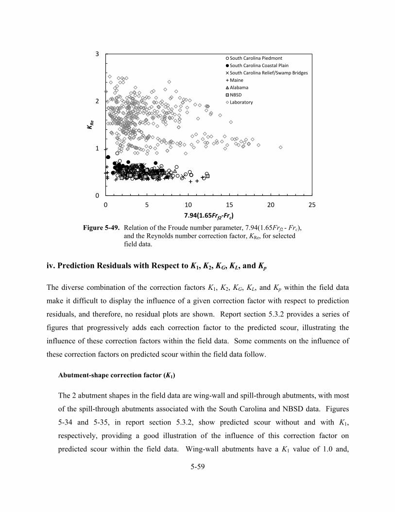
5-59
iv. Prediction Residuals with Respect to K1, K2, KG, KL, and Kp
The diverse combination of the correction factors K1, K2, KG, KL, and Kp within the field data
make it difficult to display the influence of a given correction factor with respect to prediction
residuals, and therefore, no residual plots are shown. Report section 5.3.2 provides a series of
figures that progressively adds each correction factor to the predicted scour, illustrating the
influence of these correction factors within the field data. Some comments on the influence of
these correction factors on predicted scour within the field data follow.
Abutment-shape correction factor (K1)
The 2 abutment shapes in the field data are wing-wall and spill-through abutments, with most
of the spill-through abutments associated with the South Carolina and NBSD data. Figures
5-34 and 5-35, in report section 5.3.2, show predicted scour without and with K1,
respectively, providing a good illustration of the influence of this correction factor on
predicted scour within the field data. Wing-wall abutments have a K1 value of 1.0 and,
0
1
2
3
0 5 10 15 20 25
KRe
7.94(1.65Frf2‐Frc)
South Carolina Piedmont
South Carolina Coastal Plain
South Carolina Relief/Swamp Bridges
Maine
Alabama
NBSD
Laboratory
Figure 5-49. Relation of the Froude number parameter, 7.94(1.65Frf2 - Frc), and the Reynolds number correction factor, KRe, for selected field data.
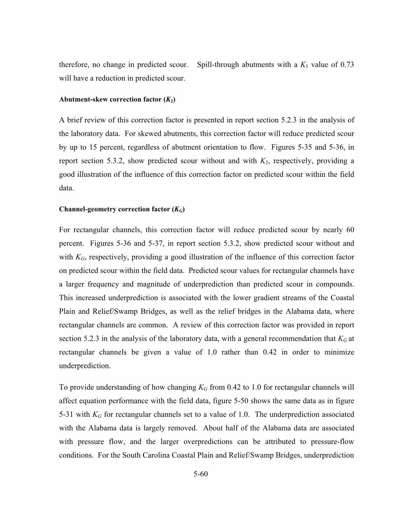
5-60
therefore, no change in predicted scour. Spill-through abutments with a K1 value of 0.73
will have a reduction in predicted scour.
Abutment-skew correction factor (K2)
A brief review of this correction factor is presented in report section 5.2.3 in the analysis of
the laboratory data. For skewed abutments, this correction factor will reduce predicted scour
by up to 15 percent, regardless of abutment orientation to flow. Figures 5-35 and 5-36, in
report section 5.3.2, show predicted scour without and with K2, respectively, providing a
good illustration of the influence of this correction factor on predicted scour within the field
data.
Channel-geometry correction factor (KG)
For rectangular channels, this correction factor will reduce predicted scour by nearly 60
percent. Figures 5-36 and 5-37, in report section 5.3.2, show predicted scour without and
with KG, respectively, providing a good illustration of the influence of this correction factor
on predicted scour within the field data. Predicted scour values for rectangular channels have
a larger frequency and magnitude of underprediction than predicted scour in compounds.
This increased underprediction is associated with the lower gradient streams of the Coastal
Plain and Relief/Swamp Bridges, as well as the relief bridges in the Alabama data, where
rectangular channels are common. A review of this correction factor was provided in report
section 5.2.3 in the analysis of the laboratory data, with a general recommendation that KG at
rectangular channels be given a value of 1.0 rather than 0.42 in order to minimize
underprediction.
To provide understanding of how changing KG from 0.42 to 1.0 for rectangular channels will
affect equation performance with the field data, figure 5-50 shows the same data as in figure
5-31 with KG for rectangular channels set to a value of 1.0. The underprediction associated
with the Alabama data is largely removed. About half of the Alabama data are associated
with pressure flow, and the larger overpredictions can be attributed to pressure-flow
conditions. For the South Carolina Coastal Plain and Relief/Swamp Bridges, underprediction
5-61
is diminished; however, substantial underprediction with some increase in overprediction is
still present. The patterns in figure 5-50 indicate that using a KG value of 1.0 for rectangular
channels will tend to reduce underpredictions and appears to be a reasonable modification to
the NCHRP 24-15(2) method.
Abutment-location correction factor (KL)
The NCHRP 24-15(2) scour prediction method includes a correction factor for abutment
location (KL) to account for potential increased scour for abutments near the channel bank or
protruding into the channel. The maximum value for KL is 1.35 and occurs when the
abutment is located at the channel bank or protrudes into the main channel. As noted in the
analysis of the laboratory data (report section 5.2.3), predicted scour associated with KL
values of 1.35 produces some of the largest overpredictions. Figures 5-37 and 5-38, in report
section 5.3.2, show predicted scour without and with KL, respectively, providing a good
3
6
15
2
4
0
10
20
30
40
50
60
0 5 10 15 20 25
Predicted abutm
ent‐scour depth, in feet
Measured abutment‐scour depth, in feet
South Carolina Relief/Swamp BridgeSouth Carolina Coastal PlainSouth Carolina PiedmontMaineAlabamaNBSD
1 Site number in Table 3‐1
Figure 5-50. Relation of predicted and measured abutment-scour depth for selected field data using the NCHRP 24-15(2) scour prediction method, with the channel-geometry correction factor, KG, set to a value of 1.0 for rectangular channels.
5-62
illustration of the influence of this correction factor on predicted scour within the field data.
The Maine and NBSD data have frequent protruding abutments, and the KL correction factor
increases the overprediction for these data, excessively so for the Maine data. Figure 5-37
shows predicted scour without KL and shows little underprediction for the Maine and NBSD
data, indicating that its inclusion is not critical in reducing underprediction at bankline and
protruding abutments. This general pattern also was confirmed in the analysis of the
laboratory data (report section 5.2.3).
An alternate method to account for the potential increases in scour for abutments near the
main channel is to use the hydraulic data associated with the channel, therefore, removing the
need for the abutment correction factor KL. This method was tested with the laboratory data,
and details regarding the method can be found in report section 5.2.3. The same approach
was tested with field data associated with bankline or protruding abutments. Figures 5-51A
and B show the relation of measured abutment-scour depth to predicted scour for the field
data with bankline or protruding abutments, with figure 5-51A reflecting computations using
the standard method for applying the NCHRP 24-15(2) method with a KL value of 1.35, and
figure 5-51B reflecting computations using the channel hydraulics with a KL value of 1.0. A
comparison of these figures indicates that using the channel hydraulic data with a KL value of
1.0 reduces the magnitude of the overpredictions with only a small increase in the frequency
and magnitude of underprediction, indicating that it likely is a reasonable alternative to
account for the potential increases in scour for abutments near the main channel.
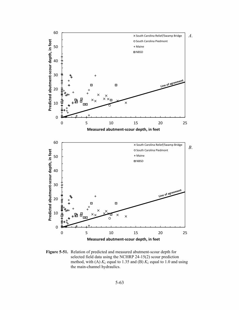
5-63
Figure 5-51. Relation of predicted and measured abutment-scour depth for selected field data using the NCHRP 24-15(2) scour prediction method, with (A) KL equal to 1.35 and (B) KL equal to 1.0 and using the main-channel hydraulics.
0
10
20
30
40
50
60
0 5 10 15 20 25
Predicted abutm
ent‐scour depth, in feet
Measured abutment‐scour depth, in feet
South Carolina Relief/Swamp Bridge
South Carolina Piedmont
Maine
NBSD
0
10
20
30
40
50
60
0 5 10 15 20 25
Predicted abutm
ent‐scour depth, in feet
Measured abutment‐scour depth, in feet
South Carolina Relief/Swamp Bridge
South Carolina Piedmont
Maine
NBSD
A.
B.
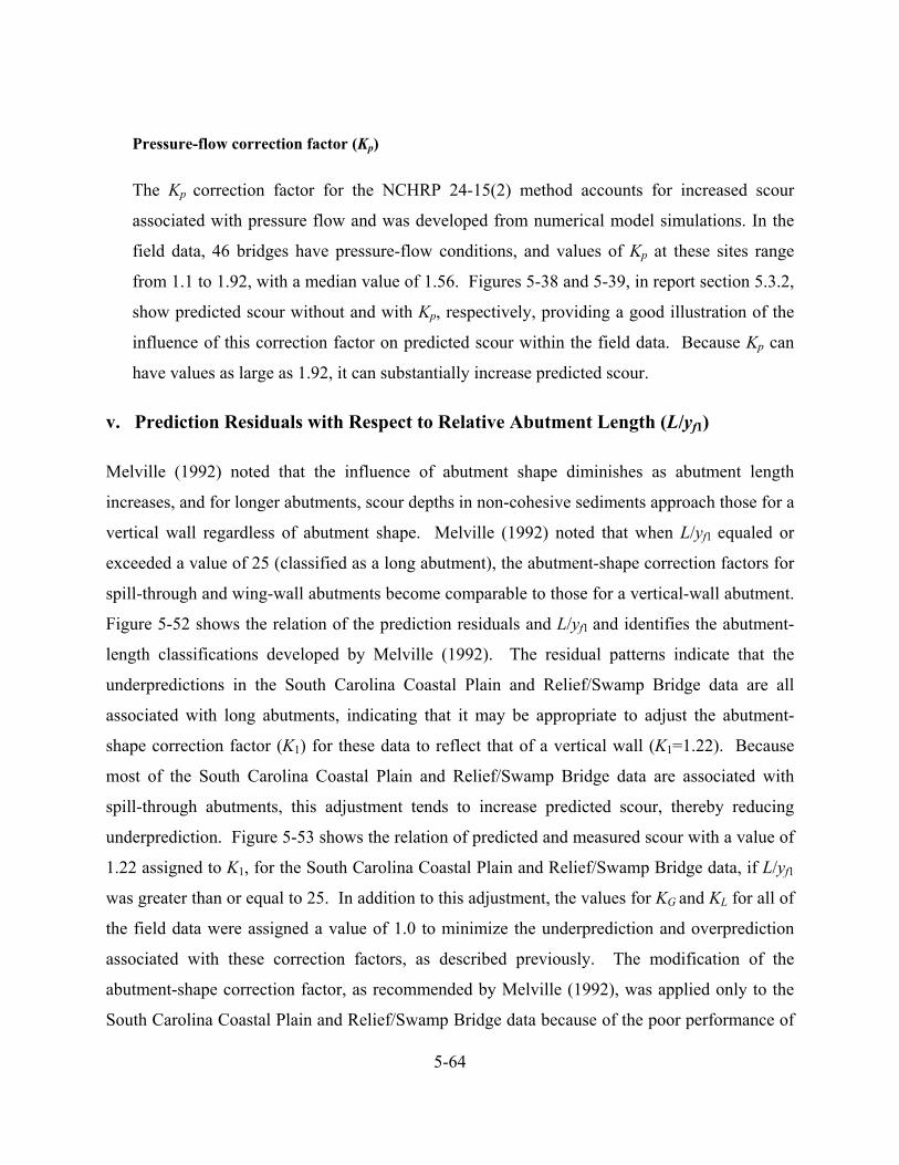
5-64
Pressure-flow correction factor (Kp)
The Kp correction factor for the NCHRP 24-15(2) method accounts for increased scour
associated with pressure flow and was developed from numerical model simulations. In the
field data, 46 bridges have pressure-flow conditions, and values of Kp at these sites range
from 1.1 to 1.92, with a median value of 1.56. Figures 5-38 and 5-39, in report section 5.3.2,
show predicted scour without and with Kp, respectively, providing a good illustration of the
influence of this correction factor on predicted scour within the field data. Because Kp can
have values as large as 1.92, it can substantially increase predicted scour.
v. Prediction Residuals with Respect to Relative Abutment Length (L/yf1)
Melville (1992) noted that the influence of abutment shape diminishes as abutment length
increases, and for longer abutments, scour depths in non-cohesive sediments approach those for a
vertical wall regardless of abutment shape. Melville (1992) noted that when L/yf1 equaled or
exceeded a value of 25 (classified as a long abutment), the abutment-shape correction factors for
spill-through and wing-wall abutments become comparable to those for a vertical-wall abutment.
Figure 5-52 shows the relation of the prediction residuals and L/yf1 and identifies the abutment-
length classifications developed by Melville (1992). The residual patterns indicate that the
underpredictions in the South Carolina Coastal Plain and Relief/Swamp Bridge data are all
associated with long abutments, indicating that it may be appropriate to adjust the abutment-
shape correction factor (K1) for these data to reflect that of a vertical wall (K1=1.22). Because
most of the South Carolina Coastal Plain and Relief/Swamp Bridge data are associated with
spill-through abutments, this adjustment tends to increase predicted scour, thereby reducing
underprediction. Figure 5-53 shows the relation of predicted and measured scour with a value of
1.22 assigned to K1, for the South Carolina Coastal Plain and Relief/Swamp Bridge data, if L/yf1
was greater than or equal to 25. In addition to this adjustment, the values for KG and KL for all of
the field data were assigned a value of 1.0 to minimize the underprediction and overprediction
associated with these correction factors, as described previously. The modification of the
abutment-shape correction factor, as recommended by Melville (1992), was applied only to the
South Carolina Coastal Plain and Relief/Swamp Bridge data because of the poor performance of
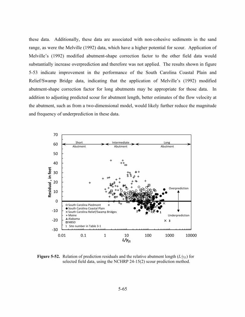
5-65
these data. Additionally, these data are associated with non-cohesive sediments in the sand
range, as were the Melville (1992) data, which have a higher potential for scour. Application of
Melville’s (1992) modified abutment-shape correction factor to the other field data would
substantially increase overprediction and therefore was not applied. The results shown in figure
5-53 indicate improvement in the performance of the South Carolina Coastal Plain and
Relief/Swamp Bridge data, indicating that the application of Melville’s (1992) modified
abutment-shape correction factor for long abutments may be appropriate for those data. In
addition to adjusting predicted scour for abutment length, better estimates of the flow velocity at
the abutment, such as from a two-dimensional model, would likely further reduce the magnitude
and frequency of underprediction in these data.
Figure 5-52. Relation of prediction residuals and the relative abutment length (L/yf1) for
selected field data, using the NCHRP 24-15(2) scour prediction method.
152
3
6
‐30
‐20
‐10
0
10
20
30
40
50
60
70
0.01 0.1 1 10 100 1000 10000
Residual , in feet
L/yf1
South Carolina PiedmontSouth Carolina Coastal PlainSouth Carolina Relief/Swamp BridgesMaineAlabamaNBSD
Overprediction
Underprediction
Long Abutment
IntermediateAbutment
ShortAbutment
1 Site number in Table 3‐1
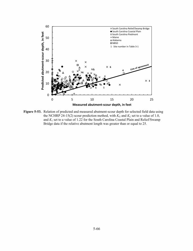
5-66
3
6
15
2
4
0
10
20
30
40
50
60
0 5 10 15 20 25
Predicted abutm
ent‐scour depth, in feet
Measured abutment‐scour depth, in feet
South Carolina Relief/Swamp BridgeSouth Carolina Coastal PlainSouth Carolina PiedmontMaineAlabamaNBSD
1 Site number in Table 3‐1
Figure 5-53. Relation of predicted and measured abutment-scour depth for selected field data using the NCHRP 24-15(2) scour prediction method, with KG and KL set to a value of 1.0, and K1 set to a value of 1.22 for the South Carolina Coastal Plain and Relief/Swamp Bridge data if the relative abutment length was greater than or equal to 25.
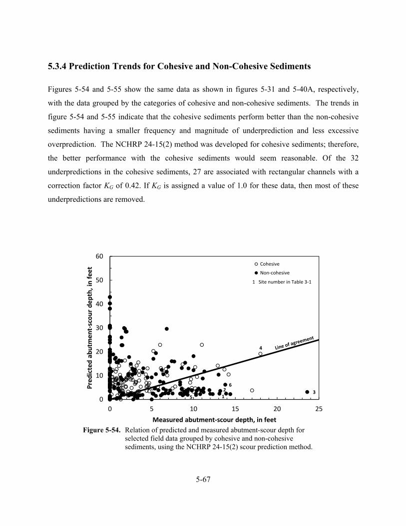
5-67
5.3.4 Prediction Trends for Cohesive and Non-Cohesive Sediments
Figures 5-54 and 5-55 show the same data as shown in figures 5-31 and 5-40A, respectively,
with the data grouped by the categories of cohesive and non-cohesive sediments. The trends in
figure 5-54 and 5-55 indicate that the cohesive sediments perform better than the non-cohesive
sediments having a smaller frequency and magnitude of underprediction and less excessive
overprediction. The NCHRP 24-15(2) method was developed for cohesive sediments; therefore,
the better performance with the cohesive sediments would seem reasonable. Of the 32
underpredictions in the cohesive sediments, 27 are associated with rectangular channels with a
correction factor KG of 0.42. If KG is assigned a value of 1.0 for these data, then most of these
underpredictions are removed.
4
15
2 3
6
0
10
20
30
40
50
60
0 5 10 15 20 25
Predicted abutm
ent‐scour depth, in feet
Measured abutment‐scour depth, in feet
Cohesive
Non‐cohesive
1 Site number in Table 3‐1
Figure 5-54. Relation of predicted and measured abutment-scour depth for selected field data grouped by cohesive and non-cohesive sediments, using the NCHRP 24-15(2) scour prediction method.
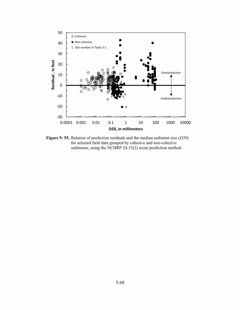
5-68
4
15
2
3
‐30
‐20
‐10
0
10
20
30
40
50
0.0001 0.001 0.01 0.1 1 10 100 1000 10000
Residual , in feet
D50, in millimeters
Cohesive
Non‐cohesive
Overprediction
Underprediction
1 Site number in Table 3‐1
Figure 5- 55. Relation of prediction residuals and the median sediment size (D50) for selected field data grouped by cohesive and non-cohesive sediments, using the NCHRP 24-15(2) scour prediction method.
5-69
5.3.5 Alternate Critical-Velocity Methods for Estimating Clear-Water
Contraction Scour
By using a similar approach to the analysis of the NCHRP 24-20 equation, alternate methods for
determining Vc were applied to the NCHRP 24-15(2) to determine their influence on equation
performance. These alternate methods include Fortier and Scobey (1926), Laursen (1963), Neill
(1973), and Vanoni (1975). A brief description of these alternate critical-velocity methods can
be found in report section 3.6. Figure 5-56 shows the relation of predicted scour to measured
scour for the data grouped by cohesive and non-cohesive sediments. The Neill (1973) method is
not shown in Figure 5-56 but performs similarly to the other methods. Figure 5-57 shows the
relation of prediction residuals (predicted minus measured scour) with respect to the median
grain size. While there are some differences, the results displayed in these figures indicate that
scour prediction, with respect to the alternate critical-velocity methods, is not highly sensitive to
the estimate of critical velocity. The influence of Vc in the NCHRP 24-15(2) method (equation 4-
1) is embedded in the parameter 7.94(1.65Frf2 – Frc) and therefore, predicted scour and Vc are
not directly proportional. The value of 1.65Frf2 is typically larger than Frc, has the stronger
influence on determining the value 7.94(1.65Frf2 – Frc), and diminishes the influence of Vc on
predicted scour.
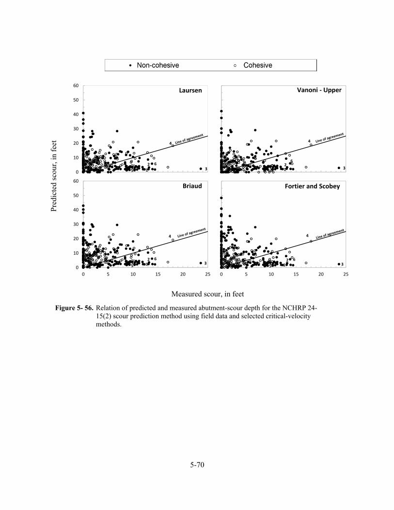
5-70
Figure 5- 56. Relation of predicted and measured abutment-scour depth for the NCHRP 24-15(2) scour prediction method using field data and selected critical-velocity methods.
4
152
3
6
0
10
20
30
40
50
60
0 5 10 15 20 25
Vanoni ‐ Upper
4
15
23
6
0
10
20
30
40
50
60
0 5 10 15 20 25
Laursen
Pre
dict
ed s
cour
, in
feet
Measured scour, in feet
4
15
23
6
0
10
20
30
40
50
60
0 5 10 15 20 25
Fortier and Scobey
4
15
23
6
0
10
20
30
40
50
60
0 5 10 15 20 25
Briaud
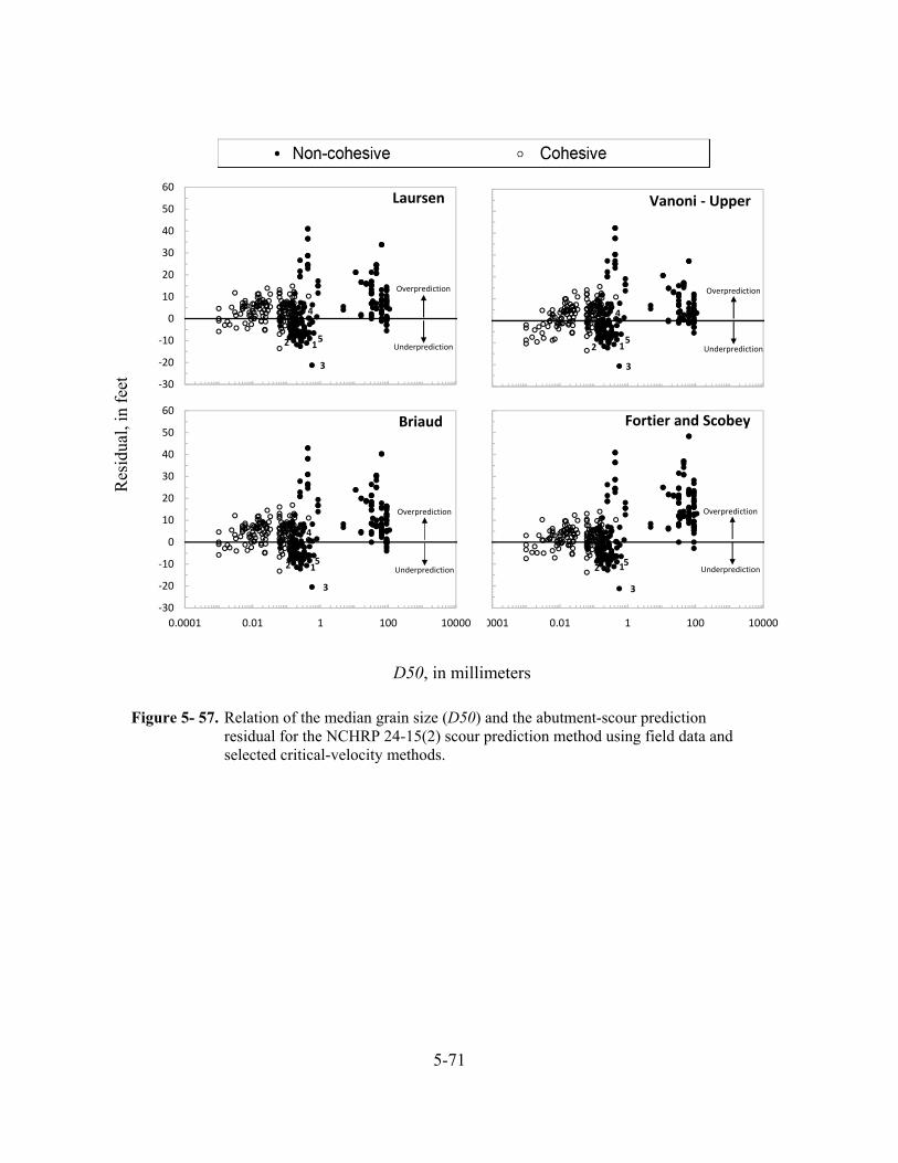
5-71
Figure 5- 57. Relation of the median grain size (D50) and the abutment-scour prediction residual for the NCHRP 24-15(2) scour prediction method using field data and selected critical-velocity methods.
4
15
2
3
‐30
‐20
‐10
0
10
20
30
40
50
60
0.0001 0.01 1 100 10000
Overprediction
Underprediction
Vanoni ‐ Upper
152
3
‐30
‐20
‐10
0
10
20
30
40
50
60
0.0001 0.01 1 100 10000
Overprediction
Underprediction
Fortier and Scobey
Res
idua
l, in
fee
t
D50, in millimeters
4
152
3
‐30
‐20
‐10
0
10
20
30
40
50
60
0.0001 0.01 1 100 10000
Overprediction
Underprediction
Laursen
4
152
3
‐30
‐20
‐10
0
10
20
30
40
50
60
0.0001 0.01 1 100 10000
Overprediction
Underprediction
Briaud
5-72
5.4 Assessment of the NCHRP 24-15(2) Prediction Method
Based on the review of the NCHRP 24-15(2) prediction method (Briaud et al. 2009; 2011) and
the analysis associated with the laboratory and USGS field data, a limited assessment of the
method is presented, including noted strengths and weakness, suggested modifications for
improved performance along with additional analysis for further verification of the method’s
performance, and limited guidance for applying the method. The complexity of scour processes
at abutments and the limitations of the data used in this analysis make it difficult to fully evaluate
the performance of the NCHRP 24-15(2) prediction method. The following comments should be
viewed in light of this challenge.
5.4.1 Strengths
The strengths of the NCHRP 24-15(2) abutment-scour prediction method include the following:
1. Simple equation form similar to the Froehlich (1989) equation:
The NCHRP 24-15(2) equation consists of a simple format that uses a series of empirical
expressions to account for the influence of a given variable on scour depth. The general
equation format is similar to the Froehlich (1989) abutment-scour equation, and the
NCHRP 24-15(2) and Froehlich (1989) equations have some similar equation parameters.
The similarity in equation form to the familiar Froehlich (1989) equation should make
application of the NCHRP 24-15(2) equation fairly intuitive to the practitioner.
2. While excessive overprediction occurs, the core explanatory variable, 7.94(1.65Frf2 –
Frc), approximates the trend of the field data with minimal underprediction:
The prediction patterns in figure 5-33 indicate that the core explanatory variable,
7.94(1.65Frf2 – Frc), captures, in some measure, the trends of the field data because
predicted scour increases as measured scour increases. While overprediction can be
excessive, there is essentially no underprediction.
5-73
3. Method performs reasonably well in cohesive sediments:
The NCHRP 24-15(2) method was originally developed for predicting abutment scour in
cohesive sediments and performs best in those types of sediments. This is particularly
evident in the cohesive sediments of the South Carolina Piedmont (figure 5-32C). The
cohesive data for Alabama (figure 5-32E) have more frequent underprediction than the
South Carolina Piermont data because they are associated with rectangular channels with
a channel-geometry correction factor, KG, that tends to cause underprediction of scour
(see report sections 5.2.4(iv) and 5.3.4). Modification of this correction factor, as noted
later in this report section, will improve performance with the Alabama data.
4. Includes a time-dependent method for a refined estimate of scour in cohesive
sediments:
While not evaluated in the current (2015) investigation, the NCHRP 24-15(2) method
includes a time-dependent method for estimating abutment scour in cohesive sediments,
providing a refined, and likely smaller, estimate of abutment scour.
5.4.2 Weaknesses
The weaknesses of the NCHRP 24-15(2) abutment-scour prediction method include the
following:
1. The method in its current format performs poorly in non-cohesive sediments:
The NCHRP 24-15(2) method was originally developed for predicting scour in cohesive
sediments, but was extended to include prediction for non-cohesive sediments. While
performance in cohesive sediments is reasonable, the method in its current format
performs poorly (figure 5-54) with substantial underprediction. If certain parameters
within the method are modified, performance in non-cohesive sediments improves
substantially.

5-74
2. The derivation of the method largely relies on empirical relations:
The derivation of the NCHRP 24-15(2) maximum abutment-scour equation (equation 4-
1) largely relies on empirical relations to define all of the equation’s explanatory
variables and does not strongly incorporate the evaluation of physics-based processes as
part of the derivation. This approach is not unusual and has been used in the derivation
of various scour prediction methods, with the Froehlich (1989) equation being a good
example of an empirically-derived equation. A weakness of this approach is that
uncertainty in the equation performance increases when applied to sites substantially
beyond the range of the data used to develop the equation. Therefore, some caution must
be used when applying the NCHRP 24-15(2) method to sites outside the range of the
dimensionless variables associated with the laboratory data used to develop the method
(table 1-4).
3. Selected correction factors need further evaluation and modification:
The analysis of the NCHRP 24-15(2) method indicates that the poor performance in the
non-cohesive sediments is related, in part, to poor definition of some of the correction
factors, including the correction factors for channel geometry, abutment location, and
abutment shape. Selected modifications of these correction factors were evaluated with
the NCHRP 24-15(2) method, and performance with the non-cohesive data improved.
These preliminary modifications are noted for consideration in the following section, but
they should be evaluated further before incorporation into the NCHRP 24-25(2) method.
.
5-75
5.4.3 Recommendations for Improving Method
The analysis of the NCHRP 24-15(2) method indicated that equation performance could improve
with modification to selected correction factors. These recommendations are based on a limited
analysis and therefore, may need additional evaluation prior to incorporating into the NCHRP
24-15(2) method.
1. Modification of the correction factor for channel geometry, KG:
The correction factor for channel geometry, KG, for rectangular channels has a value of
0.42, which increases the frequency and magnitude of underprediction at such sites. In
the field data, bridges associated with swamps and floodplain relief bridges were
classified as rectangular channels and have a much higher incidence of underprediction
(see report sections 5.3.2 and 5.3.3). The work of Melville (1992) and of Melville and
Coleman (2000) indicates that a value of 1.0 for KG at rectangular channels may be
appropriate, and this was tested in the field data (figure 5-50). Results of the test reduced
the incidence of underprediction, with some increase in overprediction. Consideration
should be given to modifying KG to a value of 1.0 for rectangular channels.
2. Modification of the correction factor for abutment location, KL:
The correction factor for abutment location, KL, accounts for potential increased scour for
abutments near the channel bank or protruding into the channel. Such sites are associated
with some of the largest overpredictions in the laboratory and field data (see report
sections 5.2.3 and 5.3.3). An alternate method to account for the potential increases in
scour is to use the hydraulic data associated with the channel, therefore removing the
need for the abutment-location correction factor KL. This alternate method was tested
with selected laboratory and field data (figures 5-30 and 5-51, respectively) and was
generally found to reduce the magnitude of the overprediction at such sites with only a
small increase in the frequency and magnitude of underprediction, indicating that it
probably is a reasonable alternative to account for the potential increases in scour for
abutments near the main channel. Consideration should be given to accounting for scour
5-76
at bankline and protruding abutments by using the channel hydraulic data rather than the
abutment-location correction factor KL.
3. Modification of the correction factor for abutment shape, K1:
The correction factor for abutment shape, K1, accounts for the influence of abutment
shape on scour depth, with streamlined shapes, such as a spill-through abutment,
producing smaller scour depths than blunt shapes, such as a vertical wall. As noted by
Melville (1992), the reduction in scour depth derived from streamlined abutment shapes
diminishes as abutment length increases, and for longer abutments, scour depths
approach those for a vertical wall regardless of abutment shape. The largest
underpredictions in the field data are associated with the long abutments of the South
Carolina Coastal Plain and Relief/Swamp Bridge data (figure 5-52) with all but 3 data
points having spill-through abutments with K1 values of 0.73. Based on the work of
Melville (1992), the K1 value for these data should be adjusted to that of a vertical wall
(1.22), which would substantially reduce underprediction (figure 5-53). Applying this
abutment-shape adjustment to the cohesive sediments of the South Carolina Piedmont
and Alabama data will substantially increase overprediction and therefore, may not be
appropriate. However, for the non-cohesive sandy sediments of the South Carolina
Coastal Plain and Relief/Swamp Bridge data, this adjustment seems appropriate.
Consideration should be given to incorporating Melville’s (1992) abutment-shape
adjustment for long abutments, in particular at sites with non-cohesive sediments similar
to those of the Coastal Plain of South Carolina. While this adjustment does not appear to
be as critical at sites with cohesive sediments, it would be beneficial to give some
consideration to its application at such sites.
4. Further evaluation of the correction factor for abutment skew, K2:
Only two abutment-scour measurements in the NCHRP 24-15(2) laboratory data were
associated with a skewed abutment, with one measurement having an abutment pointing
downstream and the other pointing upstream. Because of the limited number of data, the
relation for determining K2 should be used with caution, and further investigation of the
5-77
influence of skew on abutment-scour depth would be beneficial to confirm the equation
for determining K2 (see report section 5.2.3(iv) for additional details).
5. Further evaluation of the Reynolds number correction factor:
It is generally accepted that viscous effects, as incorporated in the Reynolds number, can
be neglected in the derivation of abutment- and contraction-scour equations (Melville and
Coleman, 2000; Sturm et al. 2011; see report section 5.2.3), thus making its inclusion in
the NCHRP 24-15(2) method problematic. The Reynolds number correction factor for
the NCHRP 24-15(2) equation was derived from a limited set of laboratory data,
including the NCHRP 24-15(2) measurements in cohesive sediments and previously
published measurements in non-cohesive sediments. Because of the limited nature of the
data used to develop this parameter, in conjunction with the previously noted observation
that viscous effects, and thus Reynolds numbers, can be neglected in the derivation of
abutment-scour equations, further evaluation of the Reynolds number correction factor
for the NCHRP 24-15(2) equation is justified. Additionally, the Reynolds numbers
associated with the field data are often much larger than those of the laboratory data used
to develop the NCHRP 24-15(2) equation (figure 5-20). In the empirical relation for KRe,
large Reynolds numbers yield smaller values of the Reynolds number correction factor
for equation 4-1, which will tend to produce smaller values of predicted scour. A
comparison of figures 5-33 and 5-34 shows how KRe substantially reduces predicted scour
in the field data. Additionally, figure 5-49 highlights the different ranges of KRe for the
laboratory and field data, showing the values for the field data to be much lower. As a
general rule, empirical and semi-empirical equations should be applied to sites having
characteristics similar to the range of the explanatory variables used to develop the
equation and should be used with caution when site conditions exceed that range.
Because most of the Ref2 values associated with the field data are substantially outside the
range of the laboratory data, in conjunction with the previously noted concerns, further
consideration should be given to testing and, if necessary, removing or modifying the
Reynolds number correction factor.
5-78
6. Evaluate the influence of Vc determined from EFA tests
The NCHRP 24-25(2) maximum abutment-scour depth equation uses an estimate of Vc
based on the empirical relation shown in figure 4-4. This relation is a lower-bound curve
of critical velocity as determined from EFA tests of field samples (Briaud et al. 2009;
2011; report section 4.2). A more accurate measurement of Vc for a given bridge site
could be obtained from EFA tests of soil samples from that site, possibly improving the
performance results for NCHRP 24-15(2). Because of the scour-resistant nature of
cohesive sediments, EFA tests may particularly reduce the overprediction associated with
these types of sediments. Therefore, it may be beneficial to test selected sites with such
data to evaluate the sensitivity of the method to the determination of Vc.
7. Safety factor
In its current format, the prediction patterns associated with the NCHRP 24-15(2) method
indicate a measure of uncertainty with frequent underprediction for larger measurements
of scour (figure 5-54). Therefore, to minimize underprediction, consideration should be
given to the incorporation of a safety factor.
8. Evaluating sensitivity to flow velocity:
Some of the underprediction in the non-cohesive sediments in the USGS field data
(figure 5-54) is likely caused by inaccurate estimates of the flow velocity from one-
dimensional flow models. It is thought that better estimates of flow velocity near the
abutment likely would improve performance, perhaps substantially. This assumption
could be evaluated by selecting a strategic sample of sites from the USGS field database,
developing two-dimensional flow models for the sites, and applying the better estimates
of flow velocity to the NCHRP 24-15(2) method. This analysis would help identify how
sensitive the NCHRP 24-15(2) method is to the estimate of flow velocity at the abutment,
providing direction for improving equation performance.

5-79
5.4.4 General Application Guidance
This guidance for application of the NCHRP 24-15(2) method is not exhaustive and is not
intended to supersede the guidance in Briaud et al. (2009; 2011):
1. Estimate of the maximum flow velocity near the abutment:
The maximum flow velocity at the abutment is an important variable in the NCHRP 24-
15(2) prediction method. A two-dimensional flow model will provide the most accurate
assessment of this variable. At bridge sites with a well-defined main channel, the
NCHRP 24-15(2) prediction method (chapter 4) provides a method to estimate a
conservative value of the maximum flow velocity at the abutment from a one-
dimensional flow model. However, this method tends to underpredict flow velocity at
the abutment for swamps and floodplain relief bridges, and a two-dimensional flow
model is a better tool for making this assessment. If a one-dimensional flow model is
used at such a site, engineering judgment should be used to estimate the larger velocity
associated with contracted flow at an abutment. In general, conservative, but reasonable,
estimates of the velocity should be used.
2. Evaluation of sediments:
The surface and subsurface sediments at a site influence the potential for abutment-scour
depth, and giving consideration to this matter is important when evaluating scour at a
bridge site. Scour depth is often limited by cohesive sediments or by subsurface scour-
resistant layers (see report section 1.2.5). However, field conditions where the depth of
the erodible sediments is very large may allow for large scour depths to develop beyond
those measured in the USGS field data. Because of the complexity of soil conditions in
the field, a multidisciplinary team, including geotechnical, structural, and hydraulic
engineers, should be used to assess the potential influence of soil conditions on scour.
5-80
3. Long abutments and large contractions:
Long abutments and large flow contractions have high potential for scour, and the
underprediction in the USGS field data is often associated with these types of site
characteristics. When such sites are being analyzed with the NCHRP 24-15(2) method, it
is important to use judgment and a strong measure of conservatism in the assessment.
Conservative estimates of flow velocity near the abutment, along with some type of
safety factor, would be advisable.
4. Application to cohesive sediments (D50 < 0.1 mm)
As noted previously (report section 5.3.4), the NCHRP 24-15(2) method performs
reasonably well with cohesive sediments. The cohesive data for Alabama will perform
well if KG is modified as noted previously in report section 5.4.3. The NCHRP 24-15(2)
method was originally developed for cohesive sediments; therefore, the better
performance with these types of sediments would seem logical. The analysis of cohesive
sediments presented in this report primarily reflects the field characteristics associated
with the South Carolina Piedmont and Alabama data. Performance of the NCHRP 24-
15(2) method in cohesive sediments may vary for sites that have characteristics beyond
the range of the South Carolina Piedmont and Alabama data. Table 1-1 provides a
summary of site characteristics associated with these data that can be used to evaluate if a
site of interest has characteristics similar to the South Carolina and Alabama data.
Additionally, the reports associated with these data (Benedict, 2003; Lee and Hedgecock,
2008) can be referenced.
5. Application to coarse sediments in the small, steep-gradient streams of Maine (D50
> 10 mm)
The small streams of Maine with steep gradients and coarse sediments (D50 > 10 mm)
have minimal underprediction, but at times excessive overprediction. The overprediction
is related to a number of factors, including the large values of Frf2 and protruding

5-81
abutments. A frequent incident of pressure flow in the Maine data will increase predicted
scour. Overprediction associated with protruding abutments can be reduced by using the
channel hydraulic data rather than the abutment-location correction factor, KL, as was
demonstrated in figure 5-51. The analysis of steep-gradient and coarse-sediment streams
presented in this report primarily reflects the characteristics associated with the Maine
data. Performance of the NCHRP 24-15(2) method for steep-gradient and coarse-
sediment streams may vary for sites that have characteristics beyond the range of the
Maine data. Table 1-1 provides a summary of site characteristics associated with these
data that can be used to evaluate if a site of interest has characteristics similar to the
Maine data. Additionally, reference can be made to the report associated with these data
(Lombard and Hodgkins, 2008).
6. Application to non-cohesive sediments in the low-gradient streams of South
Carolina
As noted previously, the NCHRP 24-15(2) method has frequent underprediction with
many of the South Carolina Coastal Plain and Relief/Swamp Bridges. These data are
generally associated with lower gradient streams with non-cohesive sandy sediments.
Wide floodplains are common at these sites, and bridges often create large contractions of
flow and thus a high potential for scour. These sites have some of the largest measured
scour depths in the field database (table 1-1), and underprediction where large scour
depths frequently occur is of concern. To minimize underprediction at such sites,
consideration should be given to modification of the correction factors K1, KG, and KL, as
previously noted. Additionally, conservative estimates of the flow velocity at the
abutment minimize the potential for underprediction, and the use of a two-dimensional
flow model may be advisable. Note that the core explanatory variable, 7.94(1.65Frf2 -
Frc), provides a conservative estimate of abutment scour in the South Carolina Coastal
Plain and Relief/Swamp Bridges (figure 5-33) with essentially no underprediction and
offers an alternative method for predicting abutment scour at sites with these
characteristics. Performance of the NCHRP 24-15(2) method in sandy, non-cohesive
sediments may vary for sites that have characteristics beyond the range of the South

5-82
Carolina Coastal Plain data. Table 1-1 provides a summary of site characteristics
associated with these data that can be used to evaluate if a site of interest has
characteristics similar to the South Carolina data, and reference can be made to Benedict
(2003) for additional information.
6-1
CHAPTER 6
COMPARISON OF RESULTS FOR NCHRP 24-20 AND NCHRP
24-15(2) AND CONCLUSIONS
6.1 Introduction
Summary statistics of prediction residuals provide a useful way to compare the performance of
selected prediction methods. Therefore, the summary statistics of the laboratory- and field-data
prediction residuals associated with the analysis of the NCHRP 24-20 and 24-15(2) prediction
methods were computed and tabulated in tables 6-1 and 6-2, respectively. (Note: The field data
for the South Carolina Coastal Plain and the Relief/Swamp Bridge data, with two exceptions, are
located in the South Carolina Coastal Plain and were combined into one group called the South
Carolina Coastal Plain for the purposes of this report section. The two exceptions are swampy
relief bridges in the Piedmont that have similar characteristics to those of the Coastal Plain data.)
The summary statistics of the prediction residuals include the minimum, mean, and maximum
values, along with the 25th, 50th, and 75th percentile values. Additionally, boxplots for the same
data listed in tables 6-1 and 6-2 were developed and are shown in figures 6-1 and 6-2, providing
a useful visual presentation of the prediction residuals. Positive values of the prediction
residuals in the boxplots represent overprediction, and negative values represent underprediction.
The scatter plots of the prediction residuals, presented earlier in the report, display the trend of
the prediction residuals with respect to a given variable, providing insights regarding prediction
trends associated with that variable. The boxplots cannot display such trends, but provide a
general understanding of equation performance and a simple tool for comparing the performance
of multiple equations. The boxplots and data in tables 6-1 and 6-2, with respect to the laboratory
and field data, are reviewed below.
6.2 Performance in the Laboratory Data
The prediction-residual boxplots in figure 6-1 indicate that the performance of the NCHRP 24-20
and NCHRP 24-15(2) prediction methods, with respect to the laboratory data, are similar in the
6-2
frequency of overprediction, with approximately 75 percent or more of the data having
overpredictions. The exception to this is the performance of the Sturm (2004) data with the
NCHRP 24-20 prediction method, where underprediction is more frequent, and comments on
this pattern will be noted later. The boxplots also indicate that the NCHRP 24-15(2) prediction
method generally has larger prediction residuals (larger overpredictions) than the NCHRP 24-20
prediction method. The magnitude of the larger overpredictions can be assessed from a review
of the data in table 6-1 and is discussed in the following sections.
6.2.1 Residual Patterns Associated with the NCHRP 24-20 Prediction Method
Some particular observations regarding the residuals in the NCHRP 24-20 prediction method are
as follows:
The Ettema et al. (2010) data have the best performance within the laboratory data, with
no underpredictions and the smallest range for the residuals. Because these data were
used to develop the NCHRP 24-20 prediction method, the pattern is to be expected and
demonstrates that the NCHRP 24-20 method reflects well the trends of the data from the
investigation.
The largest overpredictions in the NCHRP 24-20 prediction method are associated with
the cohesive sediments of the Briaud et al. (2009) data. The NCHRP 24-20 prediction
method was developed for scour prediction in non-cohesive sediments, and the larger
overpredictions in cohesive sediments are to be expected (report section 3.5). This
pattern also is observed in the field data, as is noted later.
The largest and most frequent underpredictions are associated with the Sturm (2004)
data. The Sturm (2004) data represent rigid abutments/embankments that have rigid
substructures that extend below the bed. The rigid abutment models tend to produce
larger scour depths than the erodible models of the NCHRP 24-20 investigation, and this
difference contributes to the performance patterns. Additionally, a review of tables 1-3
and 1-4 highlights the different ranges of data characteristics for the Sturm (2004) data
and the Ettema et al. (2010) data used to develop the NCHRP 24-20 prediction method.
The Sturm (2004) data include relatively long, vertical-wall abutments that are beyond
the range and characteristics of the data used to develop the NCHRP 24-20 prediction
6-3
method, providing some explanation for the differing performance. Furthermore, the
Sturm (2004) data have the smallest flow depths (tables 1-3 and 1-4) within the
laboratory data, which tend to produce smaller values of predicted scour when applied to
the NCHRP 24-20 prediction method.
Excluding the Sturm (2004) data, the non-cohesive data for Palaviccini (1993) and
Ettema et al. (2010) have a similar range of prediction residuals between the 25th and 75th
percentile (figure 6-1), with the live-bed Palaviccini (1993) data having the largest range.
A review of tables 1-3 and 1-4 highlights the similar ranges of data characteristics for
these two datasets, providing some explanation for their similar performance for the
NCHRP 24-20 prediction method.
6.2.2 Residual Patterns Associated with the NCHRP 24-15(2) Prediction
Method
Some particular observations regarding the residuals in the NCHRP 24-15(2) prediction method
are as follows:
The Briaud et al. (2009) data have no underprediction, but do have a fairly large range for
the prediction residuals. Because these data were used to develop the NCHRP 24-15(2)
prediction method, the pattern of no underprediction is to be expected. However, the
large range of the residuals, with several large overpredictions, indicates that the NCHRP
24-15(2) method, in its current form, does not fully capture the trends of these data.
The largest overpredictions in the NCHRP 24-15(2) prediction method are in the Sturm
(2004) and Ettema et al. (2010) data, displayed as outliers in figure 6-1. These data are
associated with protruding abutments that tend to produce larger overpredictions of scour
in the NCHRP 24-15(2) prediction method (report section 5.2.3), than abutments set back
from the channel. Approximately 70 percent of the Ettema et al. (2010) data have
protruding abutments, which will tend to have larger overpredictions of scour when
applied to the NCHRP 24-25(2) method. This is the primary reason why the boxplot of
the Ettema et al. (2010) data is skewed towards large overpredictions.
6-4
The NCHRP 24-15(2) prediction method produces larger overpredictions of scour in the
Sturm (2004) data in comparison to the NCHRP 24-20 prediction method. These data are
associated with larger values of Frf2 that tend to produce larger overpredictions of scour
in the NCHRP 24-15(2) prediction method (report section 5.2.3).
The Palaviccini (1993) data have some of the largest underpredictions which, in part, are
related to having rectangular channels with a channel-geometry correction factor of 0.42.
The Palaviccini (1993) live-bed data have larger overpredictions than the clear-water data
because many of the live-bed data have larger Frf2 values that tend to produce larger
scour predictions in the NCHRP 24-15(2) prediction method (report section 5.2.3).

6-5
Table 6-1. Summary statistics for the laboratory-data prediction residuals for the NCHRP 24-20 and 24-15(2) scour prediction methods.
Table 6-2. Summary statistics for the field-data prediction residuals for the NCHRP 24-20 and 24-15(2) scour prediction methods.
Live‐Bed Scour
Prediction Residuals Clear‐Water Scour Prediction Residuals
Scour Prediction Residuals
Scour Prediction Residuals
Scour Prediction Residuals
Data Source: Palaviccini (1993) Palaviccini (1993) Sturm (2004) Briaud et al. (2009) Ettema et al. (2010)
Prediction Method: NCHRP 24‐20
NCHRP 24‐15(2)
NCHRP 24‐20
NCHRP 24‐15(2)
NCHRP 24‐20
NCHRP 24‐15(2)
NCHRP 24‐20
NCHRP 24‐15(2)
NCHRP 24‐20
NCHRP 24‐15(2)
Units: (feet) (feet) (feet) (feet) (feet)
Number of data points: 164 191 74 19 40
Minimum: ‐0.73 ‐0.51 ‐0.51 ‐0.36 ‐0.91 ‐0.03 ‐1.99 0.33 0.02 ‐0.21
25th percentile: ‐0.11 0.31 ‐0.10 ‐0.05 ‐0.57 0.53 0.28 0.67 0.10 ‐0.01
Mean: 0.25 0.63 0.09 0.10 ‐0.37 0.86 0.72 0.92 0.20 0.82
Median: 0.21 0.48 0.00 0.08 ‐0.33 0.77 0.60 0.80 0.15 0.30
75th percentile: 0.58 0.94 0.25 0.19 ‐0.20 1.09 1.14 1.02 0.31 1.29
Maximum: 1.74 1.96 1.24 0.95 0.20 2.64 2.72 2.46 0.50 3.50
Standard deviation: 0.54 0.49 0.27 0.23 0.27 0.49 1.22 0.50 0.14 1.11
Scour
Prediction Residuals Scour
Prediction Residuals Scour
Prediction Residuals Scour
Prediction Residuals Scour
Prediction Residuals
Data Source: South Carolina
Piedmont South Carolina Coastal Plain Maine Alabama NBSD
Prediction Method: NCHRP 24‐20
NCHRP 24‐15(2)
NCHRP 24‐20
NCHRP 24‐15(2)
NCHRP 24‐20
NCHRP 24‐15(2)
NCHRP 24‐20
NCHRP 24‐15(2)
NCHRP 24‐20
NCHRP 24‐15(2)
Units: (feet) (feet) (feet) (feet) (feet)
Number of data points: 90 106 93 23 13
Minimum: ‐4.98 ‐3.74 ‐16.50 ‐20.47 ‐6.47 ‐5.00 ‐0.18 ‐5.84 ‐2.06 ‐0.06
25th percentile: 8.29 4.44 ‐1.57 ‐6.01 0.02 6.55 2.93 ‐1.84 0.38 4.61
Mean: 13.62 6.55 1.90 ‐1.93 3.85 14.96 6.84 ‐0.16 5.61 7.51
Median: 12.37 6.52 1.61 ‐1.99 2.63 14.79 5.85 ‐0.06 4.59 7.87
75th percentile: 17.96 8.35 4.42 0.76 5.21 21.35 9.86 1.36 6.35 9.44
Maximum: 40.17 14.52 17.29 12.79 29.02 42.91 17.47 5.49 22.40 16.89
Standard deviation: 8.18 3.49 4.97 5.69 7.08 11.38 4.99 2.57 6.85 4.45
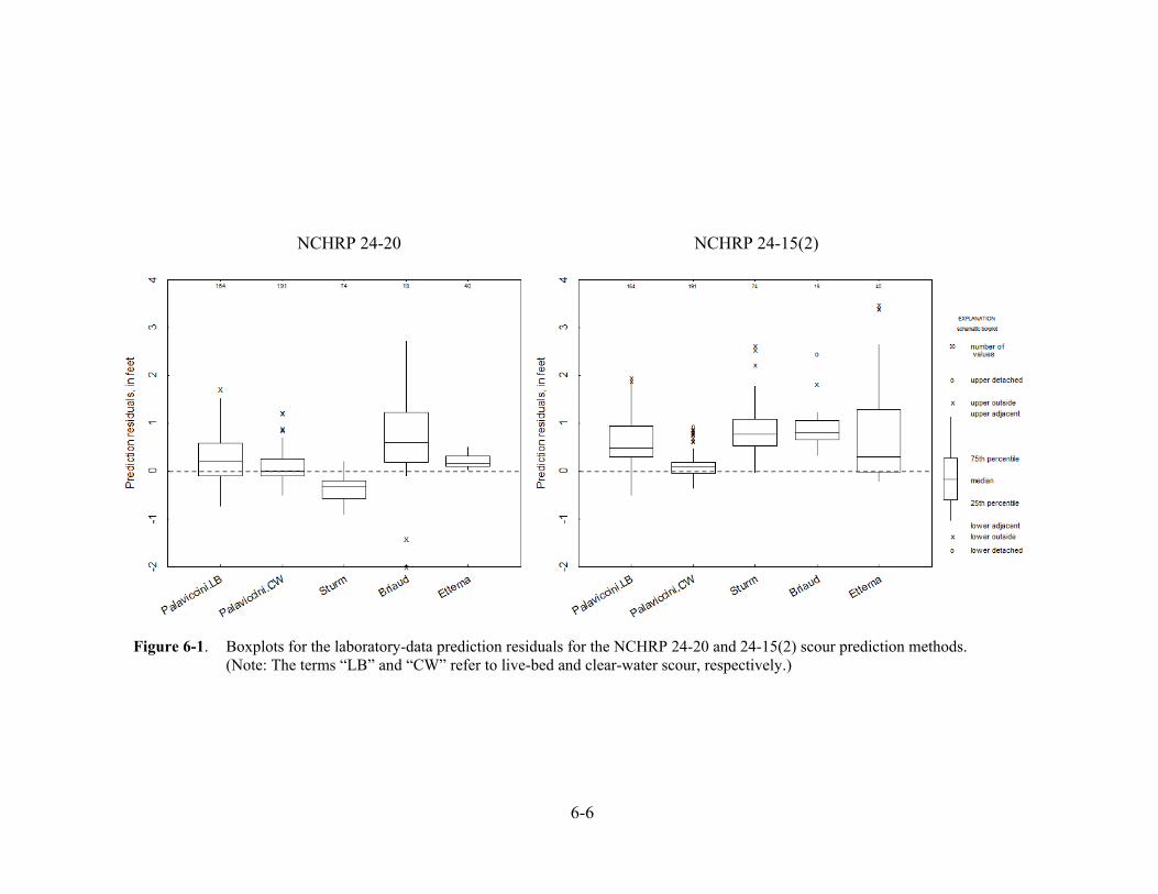
6-6
NCHRP 24-20 NCHRP 24-15(2)
Figure 6-1. Boxplots for the laboratory-data prediction residuals for the NCHRP 24-20 and 24-15(2) scour prediction methods. (Note: The terms “LB” and “CW” refer to live-bed and clear-water scour, respectively.)
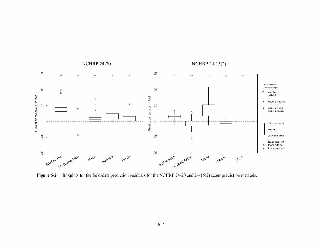
6-7
NCHRP 24-20 NCHRP 24-15(2)
Figure 6-2. Boxplots for the field-data prediction residuals for the NCHRP 24-20 and 24-15(2) scour prediction methods.
6-8
6.3 Performance in the Field Data
Similar to the performance of the laboratory data, the prediction-residual boxplots in figure 6-2
indicate that the performance of the NCHRP 24-15(2) and NCHRP 24-20 prediction methods,
with respect to the field data, tend to produce overpredictions, with approximately 75 percent or
more of the data having overpredictions. The exception to this is the performance of the South
Carolina Coastal Plain and Alabama data with the NCHRP 24-15(2) prediction method;
comments on this pattern are noted later.
6.3.1 Residual Patterns Associated with the NCHRP 24-20 Prediction Method
Some particular observations regarding the residuals in the NCHRP 24-20 prediction method are
as follows:
The largest overpredictions in the NCHRP 24-20 prediction method are associated with
the cohesive sediments of the South Carolina Piedmont. The current formulation of the
NCHRP 24-20 prediction method was developed for scour prediction in non-cohesive
sediments, and the larger overprediction in cohesive sediments is to be expected. The
cohesive sediments of the Alabama data also produce larger predicted scour depths than
the non-cohesive sediment data, but not as large as the predicted scour depths of the
South Carolina Piedmont data. The Alabama data consist of all floodplain relief bridges
that must use the average flow velocity through the bridge, rather than the more
conservative estimate of velocity associated with the SBR method (chapter 2), providing
some explanation for the smaller scour predictions. Large overpredictions also were
noted in the cohesive sediments of the Briaud et al. (2009) laboratory data (figure 6-1).
The prediction patterns in the cohesive sediments of the laboratory and field data indicate
that the NCHRP 24-20 prediction method, originally developed for scour prediction in
non-cohesive sediments, tends to produce large, and at times excessive, overprediction in
cohesive sediments. Alternate critical-velocity methods were tested in the NCHRP 24-20
prediction method (report section 3.5), and while overprediction was substantially
reduced in the cohesive sediments, underprediction increased.
6-9
The patterns of the prediction residuals for the non-cohesive sediments of the South
Carolina Coastal Plain, Maine, and NBSD data are similar, with the 25th percentile, mean,
median, and 75th percentile having comparable values (table 6-2). These data include
non-cohesive sediments ranging from small sand sizes up to coarse gravel, indicating that
the NCHRP 24-20 prediction method performs in a similar manner over a wide range of
non-cohesive sediment sizes, and is most applicable to non-cohesive sediments. The
relations of predicted and measured scour for the non-cohesive sediments of the
laboratory and field data (figures 3-1 and 3-25, respectively) generally show an
approximate symmetric scatter of the predicted values around the line of agreement,
indicating that the NCHRP 24-20 prediction method, on average, is reflecting the general
trends of the measured data for these types of sediments. However, the laboratory and
field data both indicate a trend of more frequent underprediction as the scour depth
increases. In particular, there is more frequent underprediction of scour in the field data
for measured abutment-scour depths of approximately 10 ft and larger. This trend is
highlighted in figure 6-3 where boxplots of the prediction residuals grouped by cohesive
and non-cohesive sediments, and by measured scour depth less than or greater than 10 ft,
are shown. For both sediment categories, the frequency and magnitude of
underprediction with the NCHRP 24-20 method is larger for the category of measured
scour depths greater than 10 ft, and is most severe in the non-cohesive sediments. Table
6-3 provides the summary statistics for the data in figure 6-3, again highlighting this
trend. The underpredictions associated with the non-cohesive data, in part, may be
associated with poor estimates of the flow velocity at the abutment as determined from
one-dimensional flow models. Performance would likely improve with better estimates
of the flow velocity from two-dimensional flow models. Additionally, most of the
underpredictions in the non-cohesive sediments are associated with relatively long spill-
through abutments, and incorporation of an adjustment for long abutments based on the
work of Melville (1992) likely will improve performance at these sites. Because of the
potential for underprediction for larger measured scour depths, caution and judgment is
required in the application of the NCHRP 24-20 prediction method to non-cohesive
sediments.

6-10
Recommendations for ways to potentially improve the performance of the NCHRP 24-
20 are presented in report section 5.7
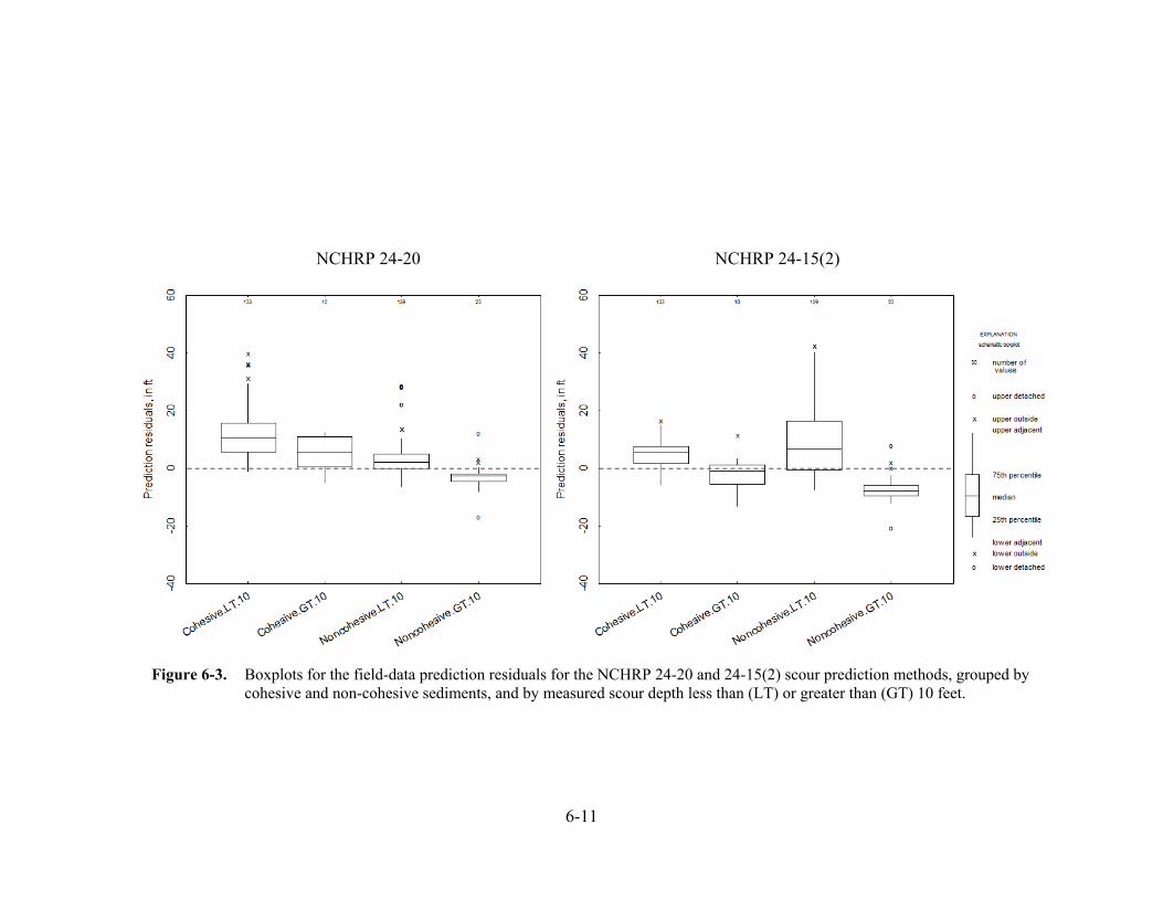
6-11
NCHRP 24-20 NCHRP 24-15(2)
Figure 6-3. Boxplots for the field-data prediction residuals for the NCHRP 24-20 and 24-15(2) scour prediction methods, grouped by cohesive and non-cohesive sediments, and by measured scour depth less than (LT) or greater than (GT) 10 feet.
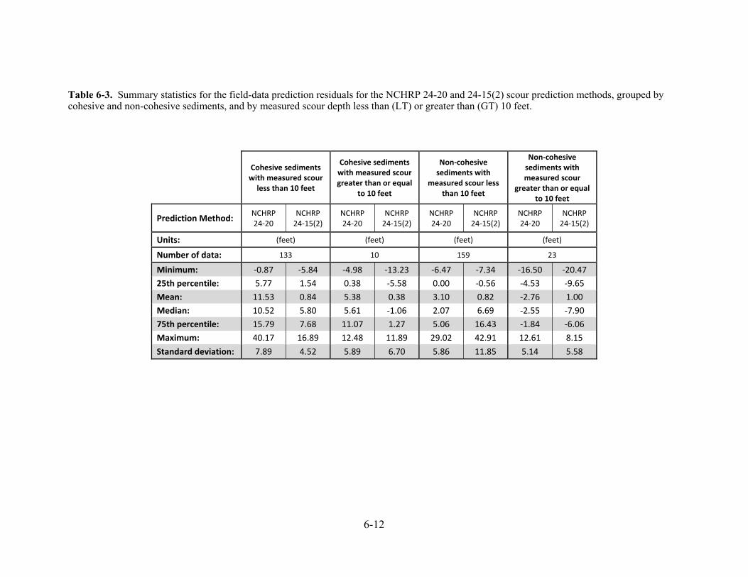
6-12
Table 6-3. Summary statistics for the field-data prediction residuals for the NCHRP 24-20 and 24-15(2) scour prediction methods, grouped by cohesive and non-cohesive sediments, and by measured scour depth less than (LT) or greater than (GT) 10 feet.
Cohesive sediments with measured scour less than 10 feet
Cohesive sediments with measured scour greater than or equal
to 10 feet
Non‐cohesive sediments with
measured scour less than 10 feet
Non‐cohesive sediments with measured scour
greater than or equal to 10 feet
Prediction Method: NCHRP 24‐20
NCHRP 24‐15(2)
NCHRP 24‐20
NCHRP 24‐15(2)
NCHRP 24‐20
NCHRP 24‐15(2)
NCHRP 24‐20
NCHRP 24‐15(2)
Units: (feet) (feet) (feet) (feet)
Number of data: 133 10 159 23
Minimum: ‐0.87 ‐5.84 ‐4.98 ‐13.23 ‐6.47 ‐7.34 ‐16.50 ‐20.47
25th percentile: 5.77 1.54 0.38 ‐5.58 0.00 ‐0.56 ‐4.53 ‐9.65
Mean: 11.53 0.84 5.38 0.38 3.10 0.82 ‐2.76 1.00
Median: 10.52 5.80 5.61 ‐1.06 2.07 6.69 ‐2.55 ‐7.90
75th percentile: 15.79 7.68 11.07 1.27 5.06 16.43 ‐1.84 ‐6.06
Maximum: 40.17 16.89 12.48 11.89 29.02 42.91 12.61 8.15
Standard deviation: 7.89 4.52 5.89 6.70 5.86 11.85 5.14 5.58
6-13
6.3.2 Residual Relations Associated with the NCHRP 24-15(2) Prediction
Method
Some particular observations regarding the residuals in the NCHRP 24-15(2) prediction method
are as follows:
The Maine data have the largest overpredictions in the NCHRP 24-15(2) prediction
method. This overprediction is attributed to larger Frf2 values and protruding abutments,
both of which tend to produce larger scour predictions in the NCHRP 24-15(2) prediction
method. As demonstrated in report section 5.3.3, using the channel hydraulic data as an
alternative to the abutment-location correction factor for protruding abutments will
reduce the magnitude of overprediction and improve performance in the Maine data.
The South Carolina Coastal Plain and Alabama data have the highest frequency of
underprediction. This underprediction, in part, may be associated with poor estimates of
the flow velocity at the abutment as determined from one-dimensional flow models, and
performance would likely improve with better estimates of the flow velocity from two-
dimensional flow models. Additionally, these data have a high frequency of floodplain
relief bridges and swamps with poorly defined channels that were classified as
rectangular channels. The channel-geometry correction factor for such sites is 0.42,
which will tend to produce more frequent underprediction. As demonstrated in report
section 5.3.3, modifying the channel-geometry correction factor from a value of 0.42 to
1.0 for rectangular channels will diminish the frequency and magnitude of
underprediction in the South Carolina data and remove underprediction from the
Alabama data. Recommendations for modifying selected correction factors in the
NCHRP 24-15(2) prediction method are presented in report section 5.4, and these
modifications substantially improve performance in the South Carolina Coastal Plain
data.
The cohesive sediments of the South Carolina Piedmont data have infrequent
underprediction. The range of the overprediction is relatively small, with a mean
prediction residual of 6.5 ft, and the 75th percentile and maximum values are 8.4 ft and
14.5 ft, respectively (table 6-2). The underprediction associated with the cohesive

6-14
sediments of the Alabama data, as noted previously, is caused by the correction factor of
0.42 for rectangular channels, which when modified to a value of 1.0, the underprediction
is removed (report section 5.3.3). The performance of the South Carolina Piedmont data
and the Alabama data, modified as suggested, indicates that the NCHRP 24-15(2)
prediction method will likely perform well in cohesive sediments. The NCHRP 24-15(2)
prediction method was originally developed for cohesive sediments, so the better
performance with the South Carolina Piedmont and Alabama data would seem logical.
As noted for the NCHRP 24-20 prediction method, there is more frequent
underprediction of scour in the field data for measured abutment-scour depths of
approximately 10 ft and larger than for measured abutment-scour depths less than 10 ft.
This trend is highlighted in the boxplots shown in figure 6-3 and in the summary statistics
for the prediction residuals in table 6.3 (see report section 6.3.1 for descriptions of figure
6-3 and table 6-3), where the frequency and magnitude of underprediction with the
NCHRP 24-15(2) method are larger for the category of measured scour depths greater
than 10 ft, and is most severe in the non-cohesive sediments. As noted for the NCHRP
24-20 method, the underprediction is likely caused by a number of factors, including poor
estimates of the flow velocity at the abutment as determined from one-dimensional flow
models and relatively long spill-through abutments that tend to produce larger scour
depths. Performance would likely improve with better estimates of the flow velocity
from two-dimensional flow models and with the incorporation of an adjustment for long
abutments based on the work of Melville (1992). Additionally, many of the non-cohesive
data are associated with rectangular channels that tend to underpredict scour because the
channel-geometry correction factor is 0.42. Modifying this correction factor to 1.0 will
substantially improve performance. Because of the potential for underprediction for
larger measured scour depths, caution and judgment are required in the application of the
NCHRP 24-15(2) prediction method to non-cohesive sediments.
Recommendations for ways to potentially improve the performance of the NCHRP 24-
15(2) method are presented in report section 5.4.
6-15
6.4 Conclusions
The NCHRP 24-15(2) and NCHRP 24-20 investigations represent extensive efforts to develop
conceptual models for abutment scour in cohesive and non-cohesive sediments, collect
laboratory data, evaluate those data, and develop new methods for predicting abutment scour.
The conceptual models, along with the data collected in these investigations, provide a valuable
resource to assist the engineer in evaluating abutment scour. The focus of the current
investigation was to evaluate the performance of these newly developed equations by using
laboratory and field data. As described earlier in the report, the laboratory and field data have
inherent weaknesses and limitations (chapter 1), and the results presented in this report will in
some measure be a function of those limitations. Therefore, caution and judgment should be used
in the evaluation, interpretation, and application of the findings in this report. However, the large
amount of data used in the investigation (tables 1-1 and 1-3) is sufficient to provide a general
understanding of each equation's performance, providing helpful information to those using these
equations. A general summary of conclusions based on the results from this report is presented in
the following report sections.
The NCHRP Project 24-27(2) (Sturm et al. 2011) reviewed selected abutment-scour research,
including the NCHRP 24-15(2) and NCHRP 24-20 prediction methods and made general
recommendations for abutment-scour design. The following quotation from that report provides
insights to the challenges that still exist for scour prediction at abutments.
Given this state of our current understanding of abutment/contraction scour, or
lack thereof, it is very difficult to develop design-specific recommendations at this
time. Some important strides forward have been made in the past decade, but
there remains much to be learned before we have arrived at the more settled and
defined state of knowledge that currently exists with respect to pier scour.
While the challenges of predicting abutment scour are real, Sturm et al. (2011) provide some
general and useful recommendations for abutment-scour design, as well as further research (see
chapter 7 of that report). The conclusions of the current (2015) investigation should be
considered in light of these recommendations.
6-16
6.4.1 Summary of Conclusions for NCHRP 24-20
Report section 3.7 provides a description of selected strengths and weaknesses associated with
the NCHRP 24-20 prediction method, and some of the more notable characteristics are
summarized below. One strength of the NCHRP 24-20 method is its simple conceptual model
derived from physical processes, in which abutment scour is considered a function of contraction
scour. The simplicity of the model provides a logical explanation of the relation between
abutment and contraction scour, and its derivation from physical processes should make the
method applicable to a broad range of field conditions. The current formulation of the NCHRP
24-20 method uses Laursen’s (1960; 1963) familiar and widely accepted contraction-scour
equations, which should make application of the NCHRP 24-20 method fairly intuitive to the
practitioner.
The performance of the NCHRP 24-20 method, as shown in figure 3-25, indicates that the
method is reflecting the general trend of the non-cohesive field data, with predicted scour depth
increasing as measured scour depth increases, particularly for measured scour depths less than
about 10 ft. This pattern suggests that the NCHRP 24-20 method is, in some measure, capturing
the scour processes for the non-cohesive field data within this range. The boxplots in figure 6-2
also highlight the performance pattern in the non-cohesive sediments. However, as measured
scour depth increases beyond 10 ft, underprediction also increases (figure 6-3), which is of
concern. Multiple factors likely contribute to this pattern of underprediction, including
limitations associated with the field and laboratory data. With regard to the field data, poor
estimates of flow velocities at the abutment from one-dimensional flow models likely causes
some of the underprediction, and performance would likely improve with better velocity
estimates from two-dimensional flow models. With regard to the laboratory data, the erodible
abutment/embankment models used to develop the NCHRP 24-20 method for Scour Condition B
(figure 3-21) eroded, producing smaller scour depths than rigid or intact abutments. Because the
USGS field data with Scour Condition B reflect intact abutments (see report section 3.4), the
NCHRP 24-20 method may tend to underpredict scour at such abutments, producing some of the
underprediction seen in figure 3-25. While eroded abutments and failed embankments are
common in the field, many abutments/embankments will remain intact during a flood. Because
of the differing scour patterns between erodible and intact abutments, the practitioner will need

6-17
to evaluate the appropriateness of using the NCHRP 24-20 prediction method for abutments with
Scour Condition B. (See report section 3.4 for additional details.) A way to address this concern
would be the inclusion of an appropriate abutment-scour countermeasure, which is recommended
as a standard design procedure by Sturm et al. (2011) for all new abutment designs. With
respect to cohesive sediments, the boxplots in figure 6-2 show the infrequent underprediction for
the cohesive sediments of the South Carolina Piedmont and Alabama, but overprediction that at
times is excessive, especially in the South Carolina Piedmont data. Additional information on
the strengths and weaknesses of the NCHRP 24-20 method can be found in report section 3.7.
While the underprediction in the non-cohesive sediments and the noted limitations associated
with the NCHRP 24-20 method are a concern, the prediction patterns in the non-cohesive
sediments displayed in figure 3-2 indicate that the method is reflecting the general trends of
abutment scour in the field and that further research and evaluation will likely yield improved
performance. Some specific areas for further evaluation are noted in report section 3.7.3 and
include:
Evaluating the sensitivity to flow velocity by using two-dimensional flow models at
selected sites in the USGS field data.
Evaluating the influence of relatively long abutments to determine if incorporating an
adjustment factor (Melville, 1992; Melville and Coleman, 2000) in the NCHRP 24-20 for
such abutments would be appropriate to minimize the potential for underprediction.
Evaluating the amplification factor for field conditions where the abutment and
embankment remains intact.
Developing an appropriate safety factor.
Developing an equation formulation appropriate for cohesive sediments.
Evaluating the current, simplified contraction-scour equations to improve these methods
that in turn will improve abutment-scour prediction.
6-18
Limited guidance for applying the NCHRP 24-20 method is presented in report section 3.7.4.
This guidance is not exhaustive and is not intended to supersede the guidance in HEC-18 or
NCHRP 24-20. Additionally, the practitioner will need to evaluate the appropriateness of using
the NCHRP 24-20 method for the given design criteria and site conditions. The guidance
provides some cautions regarding the estimate of flow velocity at the abutment, evaluation of
scour potential at long abutments and large flow contractions, and the influence of soil
conditions on scour at a given site. Additionally, limited guidance is provided for applying the
NCHRP 24-20 method to sites with cohesive sediments similar to the South Carolina Piedmont
and Alabama data, steep-gradient streams with coarse sediments similar to the Maine data, and
low-gradient streams with non-cohesive sediments similar to the South Carolina Coastal Plain
data. The performance of the NCHRP 24-20 prediction method, as presented in this report, is
based on the range of site conditions associated with the field data in table 1-1, and uncertainty
of the equation performance increases as site conditions approach the limits or deviate from
those listed in table 1-1.
6.4.2 Summary of Conclusions for NCHRP 24-15(2)
Report section 5.4 provides a description of selected strengths and weaknesses associated with
the NCHRP 24-15(2) prediction method, and some of the more notable characteristics are
summarized here. The NCHRP 24-15(2) method consists of a simple equation format similar to
the Froehlich (1989) abutment-scour equation, which should make application of the method
fairly intuitive. The prediction method was developed for cohesive sediments, and results from
this investigation indicate that the equation in its original form will perform best in those types of
sediments. The boxplots in figure 6-2 and the scatter plot in figure 5-32C highlight the good
performance in the cohesive sediments of the South Carolina Piedmont, and similar performance
occurs in the cohesive sediments of the Alabama data (figure 5-50) when the recommended
modification for rectangular channels is made. The equation in its original form does not
perform as well in the non-cohesive sediments (figure 5-54), with substantial underprediction in
the low-gradient streams of the South Carolina Coastal Plain (figures 5-32A and B) and
substantial overprediction in the steep-gradient streams with coarse sediments of Maine (figure
5-32D). Similar to the performance in the NCHRP 24-20 prediction method, the underprediction
in the South Carolina Coastal Plain, in part, is likely associated with poor estimates of the flow
6-19
velocity at the abutment as determined from one-dimensional flow models, and performance
would likely improve with better estimates of the flow velocity from two-dimensional flow
models. However, other factors likely contribute to this pattern. It is notable that the core
explanatory variable, 7.94(1.65Frf2 - Frc), provides a conservative estimate of abutment scour in
the low-gradient streams of the South Carolina Coastal Plain (figure 5-33) with essentially no
underprediction.
A review of the correction factors in the NCHRP 24-15(2) prediction method indicates that
further evaluation and modification of some of these factors may lead to improved performance.
Specific recommendations are presented in report section 5.4.3, including the following:
Modifying the value of the channel-geometry correction factor, KG, for rectangular
channels from 0.42 to 1.0.
Using the channel hydraulic data rather than the abutment-location correction factor, KL,
to account for the potential increase in scour at bankline and protruding abutments.
Incorporating an adjustment to the abutment shape correction factor, K1, to account for
the potential increase of scour associated with long abutments as described in Melville
(1992). (Note: The modification only was applied to the South Carolina Coastal Plain
data as described in report section 5.4.)
Further evaluating the correction factor for abutment skew, K2, because of the limited
data used to develop the factor.
Further evaluating the Reynolds number correction factor, KRe, to address some of the
problematic issues described in report section 5.4.3.
Evaluating the influence on predicted scour for Vc as determined from an EFA test in
contrast to Vc as determined from figure 4-4.
Evaluating the sensitivity to flow velocity by using two-dimensional flow models at
selected sites in the USGS field data.
Developing an appropriate safety factor.
6-20
Limited guidance for applying the NCHRP 24-15(2) method is presented in report section 5.4.4.
This guidance is not exhaustive and is not intended to supersede the guidance in Briaud et al.
(2009, 2011). Additionally, the practitioner will need to evaluate the appropriateness of using
the NCHRP 24-15(2) method for the given design criteria and site conditions. The guidance
provides some cautions regarding the estimate of flow velocity at the abutment, evaluation of
scour potential at long abutments and large flow contractions, and the influence of soil
conditions on scour at a given site. Additionally, limited guidance is provided for applying the
NCHRP 24-15(2) method to sites with cohesive sediments similar to the South Carolina
Piedmont and Alabama data, steep-gradient streams with coarse sediments similar to the Maine
data, and low-gradient streams with non-cohesive sediments similar to the South Carolina
Coastal Plain data. The performance of the NCHRP 24-15(2) prediction method as presented in
this report is based on the range of site conditions associated with the field data in table 1-1, and
uncertainty of the equation performance increases as site conditions approach the limits or
deviate from those listed in table 1-1.
R-1
REFERENCES
Arneson, L.A., Zevenbergen, L.W., Lagasse, P.F., and Clopper, P.E. (2012). “Evaluating Scour
at Bridges.” Hydraulic Engineering Circular No. 18, 5th Ed., Federal Highway
Administration, Arlington, VA.
Benedict, S.T. (2003). “Clear-water abutment and contraction scour in the Coastal Plain and
Piedmont Provinces of South Carolina, 1996-99.” Water-Resources Investigations Report 03-
4064, U. S. Geological Survey, Columbia, South Carolina.
Benedict, S.T. (2010). “Evaluation of Maryland abutment scour equation through selected
threshold velocity methods.” Transportation Research Record, No. 2195, pp. 153-167.
Benedict, S.T., and Caldwell, A.W. (2006). “Development and evaluation of clear-water pier and
contraction scour envelope curves in the Coastal Plain and Piedmont Provinces of South
Carolina.” Scientific Investigations Report 5289, U. S. Geological Survey, Reston, VA.
Benedict, S.T., Deshpande, N., Aziz, N.M., and Conrads, P.A. (2006). “Trends of abutment-
scour prediction equations applied to 144 field sites in South Carolina.” Open-File Report 03-
295, U. S. Geological Survey, Reston, VA.
Benedict, S.T., Deshpande, N., and Aziz, N.M. (2007). “Evaluation of abutment scour prediction
equations with field data” Transportation Research Record, No. 2025, pp. 118-126.
Briaud, J.-L., Ting, F., Chen, H.-C., Gudavalli, R., Kwak, K., Philogene, B., Han, S.-W.,
Perugu, S., Wei, G.S., Nurtjahyo, P., Cao, Y.W., and Li, Y. (1999 (a)). "SRICOS: Prediction
of Scour Rate at Bridge Piers." TTI Report no. 2937-1 to the Texas DOT, Texas A&M
University, College Station, Texas, USA.
Briaud, J.-L., Ting, F., Chen, H.C., Gudavalli, S.R., Perugu, S., and Wei, G. (1999 (b)).
"SRICOS: Prediction of Scour Rate in Cohesive Soils at Bridge Piers." ASCE Journal of
Geotechnical and Geoenvironmental Engineering Vol. 125, pp. 237-246.
Briaud, J.-L., Chen, H.-C., Li, Y., Nurtjahyo, P., and Wang, J. (2004). "Complex Pier Scour and
Contraction Scour in Cohesive Soils." NCHRP report 516, Transportation Research Board,
Washington, D.C.
Briaud, J.-L., Chen, H.-C., Chang, K.-A., Oh, S.J., and Chen, X. (2009). "Abutment Scour in
Cohesive Material." NCHRP Report 24-15(2), Transportation Research Board, National
Research Council, Washington, D.C.
R-2
Briaud, J.-L., Chen, H.-C., Chang, K.-A., Oh, S.J., Chen, S., Wang J., Li Y., Kwak K., Nartjaho
P., Gudavalli R., Wei W., Perugu S., Cao, Y.W., and Ting, F. (2011). "The SRICOS–EFA
method." Summary Report, Texas A&M University.
Brice, J.C., Blodgett, J.C., and Others (1978). “Countermeasures for hydraulic problems at
bridges, volume 2—Case histories for sites 1-283.” Report No. FHWA-RD-78-163, Federal
Highway Administration, Arlington, VA.
Chang, F., and Davis, S. (1998). "Maryland SHA procedure for estimating scour at bridge
abutments, part 2—Clear water scour," Proc. of Water Resources Engineering, '98, ASCE,
Memphis, TN, pp. 169-173.
Chang, F., and Davis, S. (1999). “Maryland SHA procedure for estimating scour at bridge
waterways, part 1—Live bed scour.” In Stream Stability and Scour at Highway Bridges,
(Eds) Richardson, E. and Lagasse, P., American Society of Civil Engineers, Reston VA, pp.
401-4011.
Conaway, J.S. (2006). “Comparison of long-term streambed scour monitoring data with modeled
values at the Knik River, Alaska,” Proc. 3rd International Conference on Scour and Erosion
at Amsterdam, Holland.
Conaway, J.S., and Brabets, T.P. (2011). “Streamflow and streambed scour in 2010 at bridge
339, Copper River, Alaska.” In Studies by the U.S. Geological Survey in Alaska, 2010 (Eds)
Dumoulin, J.A., and Dusel-Bacon,” Professional Paper 1784-C, U. S. Geological Survey,
Reston, VA.
Culbertson, D.M., Young, L.E., and Brice, J.C. (1967). “Scour and fill in alluvial channels with
particular reference to bridge sites.” Open-File Report 1967, U.S. Geological Survey.
Dongol, D.M. (1993). “Local scour at abutments.” Report 544, Dept. of Civil Engineering,
University of Auckland, Auckland, New Zealand.
Ettema, R., Nakato, T., and Muste, N. (2010). “Estimation of scour depth at bridge abutments.”
Draft final report, NCHRP Report 24-20, National Cooperative Highway Research Program,
Transportation Research Board, Washington, D.C.
Ettema, R., Yorozuya, A., Nakato, T., and Muste, M. (2005). “A practical approach to estimating
realistic depths of abutment scour.” The 2005 Mid-Continent Transportation Research
Symposium, Iowa State University, Ames, IA.
R-3
Fortier, S. and Scobey, F.C. (1926). “Permissible canal velocities,” ASCE, Transactions, Vol.
89, Paper No. 1588, pp. 940–984.
Froehlich, D.C. (1989). “Local scour at bridge abutments,” Proc. ASCE National Hydraulic
Conference, Colorado Springs, Colorado, pp. 13-18.
Hayes, D.C. (1996). “Scour at bridge sites in Delaware, Maryland, and Virginia.” Water-
Resources Investigations Report 96-4089, U.S. Geological Survey, Richmond, Virginia.
Kandasamy, J.K. (1985). “Local scour at skewed abutments.” Report No. 375, School of
Engineering, University of Auckland, Auckland, New Zealand.
Kwan, T.F. (1984). “Study of abutment scour.” Report 328, Department of Civil Engineering,
University of Auckland, Auckland, New Zealand.
Lagasse, P.F., Clopper, P.E., Zevenbergen, L.W, and Ruff, J.F. (2006). “Riprap design criteria,
recommended specifications, and quality control.” Report 568, National Cooperative
Highway Research Program, Transportation Research Board, Washington, D.C.
Lagasse, P.F., Clopper, P.E., Pagán-Ortiz, J.E., Zevenbergen, L.W., Arneson, L.A., Schall, J.D.,
and Girard, L.G. (2009). “Bridge scour and stream instability countermeasures experience,
selection, and design guidance.” Hydraulic Engineering Circular No. 23, 3rd Ed., Federal
Highway Administration, Arlington, VA.
Laursen, E.M. (1960). “Scour at bridge crossings.” J. Hydr. Div., ASCE, 86(2), 39-54.
Laursen, E.M. (1963). “An analysis of relief bridge scour.” J. Hydr. Div., ASCE, 86(2), 93-118.
Lee, K.G., and Hedgecock, T.S. (2008). “Clear-water contraction scour at selected bridge sites in
the Black Prairie Belt of the Coastal Plain in Alabama, 2006.” Scientific Investigations
Report 2007–5260 U. S. Geological Survey, Reston, VA.
Lombard, P.J., and Hodgkins, G.A. (2008). “Comparison of observed and predicted abutment
scour at selected bridges in Maine.” Scientific Investigations Report 2008–5099, U. S.
Geological Survey, Reston, VA.
Maryland State Highway Administration, Office of Structures. (2014). ABSCOUR 10, the
Maryland State Bridge Scour Program, November 2014.
Melville, B.W. (1992). “Local scour at bridge abutments.” J. Hydr. Eng., ASCE, Vol. 118, No. 4,
p. 615.
Melville, B.W. (1997). “Pier and abutment scour: Integrated approach.” Journal of Hydraulic
Engineering, ASCE, Vol. 123, No. 2, pp. 125-136.
R-4
Melville, B.W., and Coleman, S.E. (2000). “Bridge Scour.” Water Resources Publications,
Colorado, U.S.A., 550 p.
Morales, R., and Ettema, R. (2013). “Insights from depth-averaged numerical simulation of flow
at bridge abutments in compound channels,” ASCE Journal of Hydraulic Engineering, Vol.
139, No. 5, pp. 470-481.
Mueller, D.S., Miller, R.L., and Wilson, J.T. (1993). “Historical and potential scour around
bridge piers and abutments of selected stream crossings in Indiana.” Water-Resources
Investigations Report 93-4066, U.S. Geological Survey, Indianapolis, IN.
National Bridge Inventory Database (NBI). (2012). Federal Highway Administration,
Washington, D.C.
Neill, C.R. (1973). “Guide to Bridge Hydraulics.” Roads and Transportation Assoc. of Canada,
Univ. of Toronto Press, Toronto, Canada.
Palaviccini, M. (1993). “Predictor model for bridge abutments.” PhD Thesis, The Catholic
University of America, Washington, D.C.
Parola, A.C., Hagerty, D.J., and Kamojjala, S. (1998). “Highway infrastructure damage caused
by the 1993 Upper Mississippi River basin flooding.” NCHRP Report 417. National
Cooperative Highway Research Program, Transportation Research Board, Washington, D.C.
Richardson, E.V., and Davis, S.R. (2001). “Evaluating Scour at Bridges.” Hydraulic Engineering
Circular No. 18, 4th Ed., Federal Highway Administration, Arlington, VA.
Shearman, J.O. (1990). “User’s manual for WSPRO—A computer model for water-surface
profile computations.” Report No. FHWA-IP-89-027, Federal Highway Administration,
McLean, VA.
Sturm, T.W. (2004). “Enhanced abutment scour studies for compound channels.” Report No.
FHWA-RD-99-156, Federal Highway Administration, McLean, VA.
Sturm, T.W. (2006). “Scour around Bankline and Setback Abutments in Compound Channels.”
Journal of Hydraulic Engineering, ASCE, Vol. 132, No. 1, pp. 21-32.
Sturm, T.W., Ettema, R., and, Melville, B.W. (2011). “Evaluation of bridge-scour research:
Abutment and contraction scour processes and prediction.” We-Only Document 181,
National Cooperative Highway Research Program, Transportation Research Board,
Washington, D.C.
R-5
U.S. Army Corps of Engineers, (2001). “HEC–RAS River Analysis System, Hydraulic
Reference Manual.” ver. 3.1.3, Hydrologic Engineering Center, Davis, CA.
U.S. Geological Survey (2001). “National bridge scour database.” (http://water.usgs.gov/
osw/techniques/bs/BSDMS/index.html).
Vanoni, V.A. (ed.). (1975). Sedimentation Engineering, ASCE Manuals and Reports on
Engineering Practices, ASCE 54, New York, NY.
Wagner, C.R., Mueller, D.S., Parola, A.C., Hagerty, D.J., and Benedict, S.T. (2006). “Scour at
contracted bridges.” We-Only Document 83, National Cooperative Highway Research
Program, Transportation Research Board, Washington, D.C.
Yang, T.Y. (1996). “Sediment Transport Theory and Practice.” McGraw-Hill, New York.


![LTPP Data Analysis: Factors Affecting Pavement Smoothnessonlinepubs.trb.org/onlinepubs/nchrp/nchrp_w40-a.pdf · NCHRP Web Document 40 (Project 20-50[8/13]): Contractor’s Final Report](https://img.pdfslide.us/doc/110x75/5f743cc2ebc4e00f9564c732/ltpp-data-analysis-factors-affecting-pavement-nchrp-web-document-40-project-20-50813.jpg)