NCHRP 08-36, Task 115 Application of Fair Division, Data Envelopment Analysis, and Conjoint Analysis Techniques to Funding Decisions at the Program and Project/Activity Level

Nazneen Ferdous, Lauren A. Mayer, George Hart, Peter Burge and Colin Smith The RAND Corporation 1776 Main Street, P.O. Box 2138 Santa Monica, CA 90407-2138 Resource Systems Group 55 Railroad Row White River Junction, VT 05001 December, 2014

The information contained in this report was prepared as part of NCHRP Project 08-36, Task 115, National Cooperative Highway Research Program (NCHRP). Special Note: This report IS NOT an official publication of the NCHRP, the Transportation Research Board or the National Academies.

Acknowledgements This study was conducted for the AASHTO Standing Committee on Planning, with funding provided through the National Cooperative Highway Research Program (NCHRP) Project 08-36, Research for the AASHTO Standing Committee on Planning. The NCHRP is supported by annual voluntary contributions from the state Departments of Transportation. Project 08-36 is intended to fund quick response studies on behalf of the Standing Committee on Planning. The report was prepared by RAND Corporation and Resource Systems Group. The work was guided by a technical working group that included: Frank Gross, Vanassee Hangen Brustlin Feng Guo, Virginia Polytechnic Institute and State University John Milton, Washington Department of Transportation Benjamin Orsbon, South Dakota Department of Transportation Venky Shankar, Pennsylvania State University Harlan Miller, Federal Highway Administration The project was managed by Lori L. Sundstrom, NCHRP Senior Program Officer. We thank the technical working group members for the guidance and feedback on earlier drafts of this document. Additionally, we thank Michelle Horner for her administrative support.

Disclaimer The opinions and conclusions expressed or implied are those of the research agency that performed the research and are not necessarily those of the Transportation Research Board or its sponsoring agencies. This report has not been reviewed or accepted by the Transportation Research Board Executive Committee or the Governing Board of the National Research Council.

Preface

About This Document The current climate for transportation funding in the United States has resulted in an

increasing need for approaches to allocate scarce funds among transportation projects and activities. Some techniques for resource allocation that have been used by practitioners, statisticians, and economists include (a) Data Envelopment Analysis; (b) Fair Division Analysis; and (c) Conjoint analysis. All of these techniques could provide a unique approach for project prioritization and capital budgeting exercises in a state DOT environment. However, each considers and models preferences, benefits, and costs in different ways. Thus, it is important to investigate and illustratively evaluate these approaches and their ability to produce defensible and reasonable ways to allocate scarce funds. In this document, RAND and Resource Systems Group conducted a literature review of the application of these techniques in the transportation field and applied each of the techniques to a “mock” transportation capital budgeting exercise to evaluate the results. The document should be useful to state DOT transportation decision-makers who design and implement their states’ capital project development and prioritization processes to inform how and whether to use the three techniques as they work to improve the prioritization process in their states. This study was conducted for the AASHTO Standing Committee on Planning, with funding provided through the National Cooperative Highway Research Program (NCHRP) Project 08-36, Research for the AASHTO Standing Committee on Planning. The RAND Transportation, Space, and Technology Program

The research reported here was conducted in the RAND Transportation, Space, and

Technology Program, which addresses topics relating to transportation systems, space exploration, information and telecommunication technologies, nano- and biotechnologies, and other aspects of science and technology policy. Program research is supported by government agencies, foundations, and the private sector.

This program is part of RAND Justice, Infrastructure, and Environment, a division of the RAND Corporation dedicated to improving policy and decision-making in a wide range of policy domains, including civil and criminal justice, infrastructure protection and homeland security, transportation and energy policy, and environmental and natural resource policy.

Questions or comments about this report should be sent to the project leader, Lauren Mayer (Lauren@rand.org). For more information about the Transportation, Space, and Technology Program, see http://www.rand.org/transportation or contact the director at tst@rand.org.

Table of Contents

Preface............................................................................................................................................ iii About This Document ............................................................................................................................. iii

Figures........................................................................................................................................... vii Tables ........................................................................................................................................... viii Summary ........................................................................................................................................ ix 1. Introduction ................................................................................................................................. 1 2. Review of Data Envelopment Analysis in Practice .................................................................... 3

2.1 Overview ............................................................................................................................................ 3 2.2 Advantages and Disadvantages of DEA Technique ........................................................................... 5

Advantages ........................................................................................................................................... 5 Disadvantages ....................................................................................................................................... 5 Applicability to Transportation Problems ............................................................................................ 6

2.3 Application of DEA to Transportation Problems ............................................................................... 6 Efficient Use of Brazilian Airport Capacity ......................................................................................... 6 Performance of U.S. Transit Agencies ................................................................................................. 7 Performance Against Policy Goals: U.S. Bus Transit Industry ............................................................ 8 The Efficiency of Chicago Park-and-Ride Lots ................................................................................... 9 Technical Efficiency of Canadian Urban Transit Systems ................................................................. 10 North American Container Port Productivity ..................................................................................... 11 Public transport project appraisal tool in Ireland ............................................................................... 12 Performance analysis of European Airports ....................................................................................... 13

3. Review of Conjoint Analysis in Practice .................................................................................. 15 3.1 Overview .......................................................................................................................................... 15 3.2 Advantages and Disadvantages of CA Technique ............................................................................ 17

Advantages ......................................................................................................................................... 17 Disadvantages ..................................................................................................................................... 18

3.3 Application of CA for Prioritizing Transport Infrastructure Investments ........................................ 18 Puget Sound Regional Council Transportation Project Prioritization ................................................ 19 European Transport Infrastructure Investments Prioritization ........................................................... 22 CA/SP Methods as an Alternative to Analytical Hierarchy Process (AHP) for Obtaining Criteria

Weights ........................................................................................................................................ 24 4. Review of Fair Division Analysis in Practice ........................................................................... 25

4.1 Overview .......................................................................................................................................... 25 4.2 Advantages and Disadvantages of FDA Technique ......................................................................... 27

Advantages ......................................................................................................................................... 27 Disadvantages ..................................................................................................................................... 27 Applicability to Transportation Problems .......................................................................................... 27

iv

4.3 Application of FDA in Transportation Problems ............................................................................. 27 Texas Department of Transportation .................................................................................................. 28

5. Preparation of a hypothetical plan ............................................................................................ 29 5.1 Introduction ...................................................................................................................................... 29 5.2 Evaluation Criteria ............................................................................................................................ 29 5.3 Application of Each Technique: Selected Methods .......................................................................... 33

Data Envelopment Analysis ............................................................................................................... 33 Conjoint Analysis ............................................................................................................................... 34 Fair Division Analysis ........................................................................................................................ 34

6. Hypothetical Case Studies ........................................................................................................ 35 6.1 Introduction ...................................................................................................................................... 35 6.2 Case Study 1: Hypothetical Case Study Using DEA and CA Techniques ....................................... 35 6.3 Case Study 2: Hypothetical Case Study for FDA Technique ........................................................... 40

7. Application of DEA, CA, and FDA techniques ........................................................................ 43 7.1 Introduction ...................................................................................................................................... 43 7.2 Data Envelopment Analysis (DEA) ................................................................................................. 43

Modeling Project Attributes ............................................................................................................... 44 A simple DEA analysis – one input and one output ........................................................................... 44 A more sophisticated DEA analysis ................................................................................................... 46 More Attributes than Projects ............................................................................................................. 46 Categorical Attributes......................................................................................................................... 47 Negative Attribute Values .................................................................................................................. 47 Undesirable Outputs ........................................................................................................................... 48 An economic analysis of transportation projects using DEA ............................................................. 48

7.3 Conjoint Analysis ............................................................................................................................. 50 Create an Experimental Design and Collect Data .............................................................................. 50 Calculate Weight for Each Performance Measure ............................................................................. 53 Evaluate the Case Study ..................................................................................................................... 54

7.4 Fair Division Analysis ...................................................................................................................... 59 7.5 Advantages and Limitations of DEA, CA, and FDA applications ................................................... 64

Accommodating both quantitative and qualitative performance measures ........................................ 64 Accommodating performance measures that may take negative values ............................................ 64 Sensitivity to decision-makers’/stakeholders’ preferences................................................................. 64 Ease of implementation: data collection, sample size, and data analysis ........................................... 64 Ease of implementation: availability of literature, software, and other resources.............................. 65 Handling large numbers of projects ................................................................................................... 66 Level of expertise required ................................................................................................................. 66 Flexibility ........................................................................................................................................... 67

Appendix A: A Guide for Interviews with Experts and DOT Practitioners to Aid the Preparation of a Hypothetical Evaluation and Prioritization Plan ............................................................. 69

Task 2 Scope: Preparation of a hypothetical evaluation and prioritization plan .................................... 69 Task 3: Implementation of a hypothetical evaluation and prioritization plan ........................................ 69

v

Expert Interviews .................................................................................................................................... 70 State DOT Interviews ............................................................................................................................. 71

Appendix B: Performance Measure Levels Used in CA Experimental Design ........................... 73 Appendix C: Application of CA and FDA to Non-Transportation Problems .............................. 76

C.1 Conjoint Analysis Applications ....................................................................................................... 76 Stated Preference Study in Zurich ...................................................................................................... 76 Denali National Park and Preserve ..................................................................................................... 77 Okefenokee Wilderness ...................................................................................................................... 79 Isle Royale National Park ................................................................................................................... 80 Feasibility of CA as a tool for prioritizing innovations for implementation in UK health care ......... 81 Application of discrete choice modeling (DCM) to clinical service developments in Scotland ........ 82

C.2 FDA Applications ............................................................................................................................ 84 Water Distribution in Kabylia, Algeria .............................................................................................. 84 Water Distribution in Alberta, Canada ............................................................................................... 84 Assignment of Software Engineering Projects ................................................................................... 85 The Winsor Family Silver .................................................................................................................. 86 The Pope Family Furniture and Household Items .............................................................................. 87 Budget al.location for the European Union’s rural-development policy in Poland ........................... 88 Resolving an Italian insurance allocation problem ............................................................................ 89

References ..................................................................................................................................... 91

vi

Figures

Figure 2.1. Relative efficiency of supermarkets using DEA (Cooper 2007) .................................. 4 Figure 3.1. Example of a Conjoint Based Choice (CBC) Experiment ......................................... 17 Figure 3.2. Prioritization Outcomes and Performance Measures ................................................. 20 Figure 3.2. Overall Importance of Measures ................................................................................ 21 Figure 3.4. Project Scores - Before and After Cost Screening ..................................................... 22 Figure 5.2. Simple variable-returns-to-scale DEA model with efficient frontier shown

(magnified) ............................................................................................................................ 46 Figure 7.5. Screenshot of a CBC Experiment – Example 2 .......................................................... 53 Figure 7.6. Relative Preference and Rank among the Projects ..................................................... 56 Figure 7.7. FDA Process Applied for the Study ........................................................................... 60

vii

Tables

Table 2.1. Supermarket inputs (employees, floor space) in terms of outputs (sales) (Cooper 2007) ....................................................................................................................................... 4

Table 5.1. (Hypothetical) Project Evaluation and Prioritization Criteria ..................................... 31 Table 6.1. Project-level data availability by performance measures ............................................ 38 Table 6.2. Mean SDDOT Resident and Legislator Importance Ratings for Selected

Improvements on a Scale for 1 (very unimportant) to 5 (very important)............................ 41 Table 7.1. Inputs and outputs for economic analysis using DEA ................................................. 48 Table 7.2. DEA analysis results for alternative transportation projects ....................................... 49 Table 7.3. MNL Model Estimation Results .................................................................................. 55 Table 7.4. Top Three Performance Measures by Contribution to Overall Project Rating

(performance measures with counterintuitive parameter signs are excluded) ...................... 57 Table 7.5. Beneficiary Estimates, Upper and Lower Bounds used for FDA Application ............ 61 Table 7.6. Standardized Preference Rating for Each Stakeholder Group and Resultant Ordering

of Project Payment ................................................................................................................ 62 Table 7.7. Final Payment Allocation to each Project .................................................................... 63 Table 7.8. Sensitivity Analysis: Percent Change in Base Payment Allocation Resulting from

Indicated Percent Change in Assumption ............................................................................. 63

viii

Summary

The current climate for transportation funding in the United States has resulted in an increasing need for approaches to allocate scarce funds among transportation projects and activities. Some techniques for resource allocation that have been used by practitioners, statisticians, and economists include (a) Data Envelopment Analysis; (b) Fair Division Analysis; and (c) Conjoint analysis. All of these techniques could provide a unique approach for project prioritization and capital budgeting exercises in a state DOT environment. However, each considers and models preferences, benefits, and costs in different ways. Thus, it is important to investigate and illustratively evaluate these approaches and their ability to produce defensible and reasonable ways to allocate scarce funds. In this document, RAND conducted a literature review of the application of these techniques in the transportation field and applied each of the techniques to a “mock” transportation capital budgeting exercise to evaluate the results. The document should be useful to state DOT transportation decision-makers who design and implement their states’ capital project development and prioritization processes to inform how and whether to use the three techniques as they work to improve the prioritization process in their states.

Data Envelopment Analysis (DEA) is an empirical method used to evaluate the relative performance of different entities, or Decision Making Units (DMUs). Each DMU is characterized by a set of inputs and outputs in which the ratio of the outputs to the inputs provides the efficiency of a given DMU. An objective and consistent weighting scheme is applied to the inputs and outputs by comparing each DMU to the most efficient DMUs, or those DMUs that are located on the efficiency frontier. In this way, each DMU is assigned an efficiency score, allowing the relative performance of the DMUs to be compared and analyzed. DEA has been used to identify inefficient performers across many different applications and industries, including banking, health care, education, retail, and transportation.

Fair Division Analysis (FDA) encompasses a broad array of methods and application forms. The basic tenet is that criteria can be used to define a “fair” allocation of a finite resource and approaches then can be used to perform that allocation in a way that meets those criteria. Relatively simple solutions are available for divisions between two entities, but the problem becomes more complex with more than two entities. Much of the conceptual work on fair division has been done by mathematicians who have developed approaches that produce fair division under particular criteria and for different numbers of entities among whom the allocations must be made. The applications of fair division have ranged widely, from the classic cake-cutting problem and its more important real-world analogs to the problem of creating “fair” redistricting boundaries. Fair division methods could be used to assist in capital budgeting in several possible ways, some of which require assignment of subjective values (or utilities) to the

ix

items to be allocated. These approaches could use either a bidding process or a hybrid conjoint approach to determine the values that different entities assign to the projects being selected in a given budget-allocation process.

Conjoint Analysis (CA) also has a broad array of methods and applications, but is most commonly used in market research applications to estimate the relative importance of a set of attributes related to a product or service. A group of decision-makers, or respondents, is shown a controlled set of hypothetical products or services defined by a set of attributes and asked to choose their preferred alternative given varying attribute values. Discrete choice modeling techniques then can be used to estimate the relative importance of the attributes presented.

This document describes the application of DEA, CA, and FDA techniques to mock case studies in order to evaluate and compare the techniques across a set of criteria, including:

• Accommodating both quantitative and qualitative performance measures • Accommodating performance measures that may take negative values • Sensitivity to decision-makers’/stakeholders’ preferences • Handling of large number of projects • Ease of implementation, flexibility, and level of expertise required.

To undertake this evaluation we used a project/program evaluation plan with 24 performance

measures that fall under the following eight goals:

• Promote/support economic growth • Improve mobility • Sustainable environment • Safety • Social responsibility • Create/support an inclusive community • Consistent with local/regional/state plans • Return on investment. While these goals do not correspond to objectives of any specific agency, we identified the

above goals to include a broad range of criteria that reflect traditional measures as well as “soft” measures that are being increasingly employed by DOTs across the country. Also, the selected goals closely follow the MAP-21 national goals and will help states to transition towards a more performance-based program. In addition, the following points were taken into consideration in the specification of the plan/evaluation framework:

• Evaluation criteria should be meaningful, easy to understand, relatively common across the DOTs, and have data requirements that are reasonably easy to collect.

• An agency may select projects and programs simply because they are likely to make noticeable contributions towards achieving agency’s goals and objectives.

x

• Project selection committees typically include members who represent a wide range of interests and perspectives such as public transport, freight, and sustainable community. An effective evaluation framework must incorporate their interests.

• Very few alternative projects are evaluated based solely on qualitative benefits. Therefore, it is imperative that evaluation criteria should include both qualitative and quantitative measures to adequately represent policies of interest.

During this task, the team reached out and interviewed two groups of users: (1) professionals who are considered by their peers to be expert in the fields of DEA, FDA, and CA, and (2) DOT practitioners. Feedback from the experts and the DOT staffs provided valuable information in the development of the plan and case studies. Specifically, two hypothetical case studies were defined: case study 1 (for the DEA and CA techniques) and case study 2 (for the FDA technique). We needed to identify two separate case studies because FDA requires different types of inputs from DEA and CA. Application of the FDA technique requires direct input from decision-makers and stake-holders on the candidate projects to determine how limited resources may be allocated, while application of the DEA and CA techniques require detailed information on each project so that the set of performance measures identified previously may be calculated. These case studies are:

• Case study 1 for DEA and CA techniques: This case study includes the following ten projects:

1. Light rail extension (P1) 2. Bus rapid transit (P2) 3. Arterial widening (P3) 4. Interstate widening (P4) 5. Interstate pavement rehabilitation (P5) 6. Arterial pavement rehabilitation (P6) 7. Peak shoulder management (P7) 8. Vanpool expansion (P8) 9. Add more lanes (P9) 10. Modify interchange (P10).

We selected the above projects because they represent a good cross-section in terms of modes (auto versus transit), contributions to network capacity (infrastructure expansion versus infrastructure maintenance), and potential conflict of interests (for example, interstate widening versus light rail extension). The projects were selected from a number of geographic locations. To carry out the DEA and CA analyses, each project was described as completely as possible using a blend of real and simulated data.

• Case study 2 for FDA technique: This case study includes the following seven projects: 1. Expanding public transportation/bus service 2. Expanding transportation services for seniors and persons with disabilities 3. Relieving traffic congestion in cities such as Sioux Falls and Rapid City 4. Adding turning and passing lanes to highways

xi

5. Repairing and maintaining existing highways 6. Improving passenger bus service between cities 7. Improving the draining of water from the surface of highways when it rains.

South Dakota DOT (SDDOT) provided data describing the above projects. Finally, each technique was applied to evaluate the corresponding case study. A brief

description of each analysis and results is provided below.

• DEA analysis: Application of DEA involved comparing the ratio of outputs to inputs for each project. The DEA technique can only be applied if the number of projects to be evaluated is more than the number of performance measures/output. To ensure that, only the following three performance measures were treated as output: jobs created, travel time savings, and freight travel time savings. For input, annualized operating cost of each project was used. Only five projects, out of ten, were considered efficient by DEA. These projects are light rail extension (P1), bus rapid transit (P2), arterial widening (P3), interstate widening (P4), and modify interchange (P10).

• CA analysis: Application of CA involved designing a special web-based survey to elicit information about trade-offs between the performance measures. The survey link was sent to a number of DOTs including Colorado, Kansas, Michigan, Minnesota, New Mexico, North Carolina, Oregon, South Dakota, Washington, and Wyoming. In each trade-off exercise, the respondents were presented with two projects defined by six performance measures. The respondents were asked to select one project, assuming that these were their only choices. Each respondent participated in 20 trade-off exercises. In total, 11 complete survey responses were received. The data collected from the survey was used to calculate the weight of each performance measure, which then was used to calculate the utility/relative rating of each project. In this regard, one important point should be noted. Though the sample size may be considered adequate for the purpose of the current study, which is to demonstrate the applicability of the CA technique, it was not possible to obtain consistent estimates of the weights. Accordingly, results obtained from the CA analysis should be treated with care. That being said, the results of the CA analysis indicate the following order of the projects (from the most preferred to the least preferred): P1, P7, P10, P5, P8, P2, P9, P6, P3, and P4.

• FDA analysis: There are three sets of data/information needed to conduct the FDA analysis: 1) stakeholder preferences for a set of projects, 2) estimated number of beneficiaries for each of those projects, and 3) an objective unit of payment per beneficiary. To obtain a set of projects and associated stakeholder preferences, we used the results of a SDDOT Customer Satisfaction Survey, as outlined in Section 2.3. Beneficiary numbers were estimated using selected U.S. Census Data, as well as other data. The unit of payment per beneficiary ($32.75) was determined as a function of the average per capita state and local taxes in South Dakota. Upper bounds (equal to the product of the number of beneficiaries and the unit of payment) and lower bounds (chosen as 10 percent of the upper bound) for each project were determined. The payments for projects was calculated as a fraction of the upper bound for that project that is proportional to beneficiaries’ relative preference for that project. All projects received an amount at least equal to that of its lower bound and no project received more financing than its upper bound.

xii

The results of the analysis indicate several advantages and limitations of each technique:

• Data Envelopment Analysis (DEA): Though DEA can tolerate any number of inputs, outputs, and decision making units, including a large number of inputs and outputs in the model increases the likelihood of a larger set of DMUs appearing efficient. Also, DEA is not well-suited for qualitative input and output data.

• Conjoint Analysis (CA): One of the key advantages of this method is that the feature weights that are calculated using CA directly reflect the preferences of the decision-makers or other stakeholders who complete the survey exercises. CA works especially well for calculating weights for up to about 10 features. However, special approaches are needed to deal with applications involving a large numbers of features (10 plus).

• Fair Division Analysis (FDA): One primary advantage of (some rules-based) fair division analyses over other allocation methods is that a solution may be obtained without the use of a numerical computation tools. On the other hand, it is possible that the customizable nature of fair division rules and objective function may impose a level of unchecked subjectivity to an allocation solution.

Comparing these techniques across our evaluation criteria, we find further advantages

and disadvantages: • Accommodating both quantitative and qualitative performance measures: The

evaluation framework applied in the current study included several qualitative categorical measures. Of the three techniques considered here, CA was the only one that was able to accommodate these performance measures (FDA cannot accommodate any performance measures, and DEA would have required additional assumptions and data transformation).

• Accommodating performance measures that may take negative values: Again, CA was the only one able to accommodate negative value performance measures.

• Sensitivity to decision-makers’/stakeholders’ preferences: CA and FDA are fairly sensitive to decision-makers’/stakeholders’ preferences. This could be considered both an advantage and limitation as the decision-makers’/stakeholders’ understanding of the scale of the decision-making plays a key role in the final outcomes.

• Handling of large number of projects: In general, all three techniques considered in the current study are able to handle large numbers of projects, but it should be noted that an increase in the number of projects would also increase the data collection burden on the DOT staffs.

• Ease of implementation, flexibility, and level of expertise required: All three techniques present some challenges. For instance, implementing DEA and CA require a certain level of knowledge, expertise, and training. In this regard, rules-based FDA has an advantage as the technique may be implemented without any special expertise. However, the approach relies on stakeholder survey data, which must be obtained in advance. In addition, the approach applied in the current study relies on obtaining the number of beneficiaries for each project.

In summary, whether or not a particular technique may be employed in the context of developing Statewide Transportation Improvement Programs (STIPs) depends on a number of factors, including the type and the number of performance measures to be considered;

xiii

availability of data for each project; identification of appropriate beneficiaries; level of expertise; and knowledge of DOT staffs.

xiv

1. Introduction

One of the key challenges faced by state Department of Transportation (DOT) decision-makers is how best to allocate scarce funds among transportation projects and programs that offer the most benefits to the community. This involves selecting only a limited number of projects from a large number of candidate projects to be included in the Statewide Transportation Improvement Program (STIP). Practitioners, statisticians, and economists use several techniques to allocate finite resources in a fair and objective manner across many different types of applications. For this research, the following three techniques were evaluated:

• Data Envelopment Analysis (DEA) • Conjoint Analysis (CA) • Fair Division Analysis (FDA).

The objective of the current research project is to apply the resource allocation techniques listed above to a “mock” transportation capital budgeting exercise and to evaluate the results. It is envisioned that the findings of this research will provide an understandable and usable reference for the state DOT transportation decision-makers. It is hoped the findings can inform them about how to use the three techniques as they work to improve the design and implementation of their states’ capital project development and prioritization process.

This report documents the results of the current research. Specifically, after this introduction, the report is divided into the following two parts; each part includes a number of chapters:

• Part I (a review of DEA, CA, and FDA techniques in practice) includes the following chapters:

− Chapter 2 presents a review of DEA in practice − Chapter 3 contains a review of CA in practice − Chapter 4 summarizes a review of FDA in practice.

• Part II (preparation and implementation of a hypothetical evaluation and prioritization plan) includes the following chapters:

− Chapter 5 presents a hypothetical plan − Chapter 6 presents the hypothetical case studies to be evaluated − Chapter 7 discusses the application of DEA, CA, and FDA techniques − Chapter 8 provides a summary and conclusions.

1

2. Review of Data Envelopment Analysis in Practice

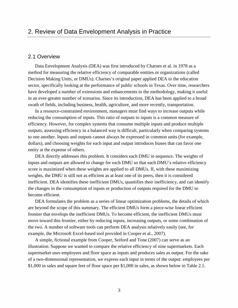
2.1 Overview Data Envelopment Analysis (DEA) was first introduced by Charnes et al. in 1978 as a

method for measuring the relative efficiency of comparable entities or organizations (called Decision Making Units, or DMUs). Charnes’s original paper applied DEA to the education sector, specifically looking at the performance of public schools in Texas. Over time, researchers have developed a number of extensions and enhancements to the methodology, making it useful in an ever-greater number of scenarios. Since its introduction, DEA has been applied to a broad swath of fields, including business, health, agriculture, and more recently, transportation.

In a resource-constrained environment, managers must find ways to increase outputs while reducing the consumption of inputs. This ratio of outputs to inputs is a common measure of efficiency. However, for complex systems that consume multiple inputs and produce multiple outputs, assessing efficiency in a balanced way is difficult, particularly when comparing systems to one another. Inputs and outputs cannot always be expressed in common units (for example, dollars), and choosing weights for each input and output introduces biases that can favor one entity at the expense of others.

DEA directly addresses this problem. It considers each DMU in sequence. The weights of inputs and outputs are allowed to change for each DMU so that each DMU’s relative efficiency score is maximized when these weights are applied to all DMUs. If, with these maximizing weights, the DMU is still not as efficient as at least one of its peers, then it is considered inefficient. DEA identifies these inefficient DMUs, quantifies their inefficiency, and can identify the changes in the consumption of inputs or production of outputs required for the DMU to become efficient.

DEA formulates the problem as a series of linear optimization problems, the details of which are beyond the scope of this summary. The efficient DMUs form a piece-wise linear efficient frontier that envelops the inefficient DMUs. To become efficient, the inefficient DMUs must move toward this frontier, either by reducing inputs, increasing outputs, or some combination of the two. A number of software tools can perform DEA analysis relatively easily (see, for example, the Microsoft Excel-based tool provided in Cooper et al., 2007).

A simple, fictional example from Cooper, Seiford and Tone (2007) can serve as an illustration. Suppose we wanted to compare the relative efficiency of nine supermarkets. Each supermarket uses employees and floor space as inputs and produces sales as output. For the sake of a two-dimensional representation, we express each input in terms of the output: employees per $1,000 in sales and square feet of floor space per $1,000 in sales, as shown below in Table 2.1.

3

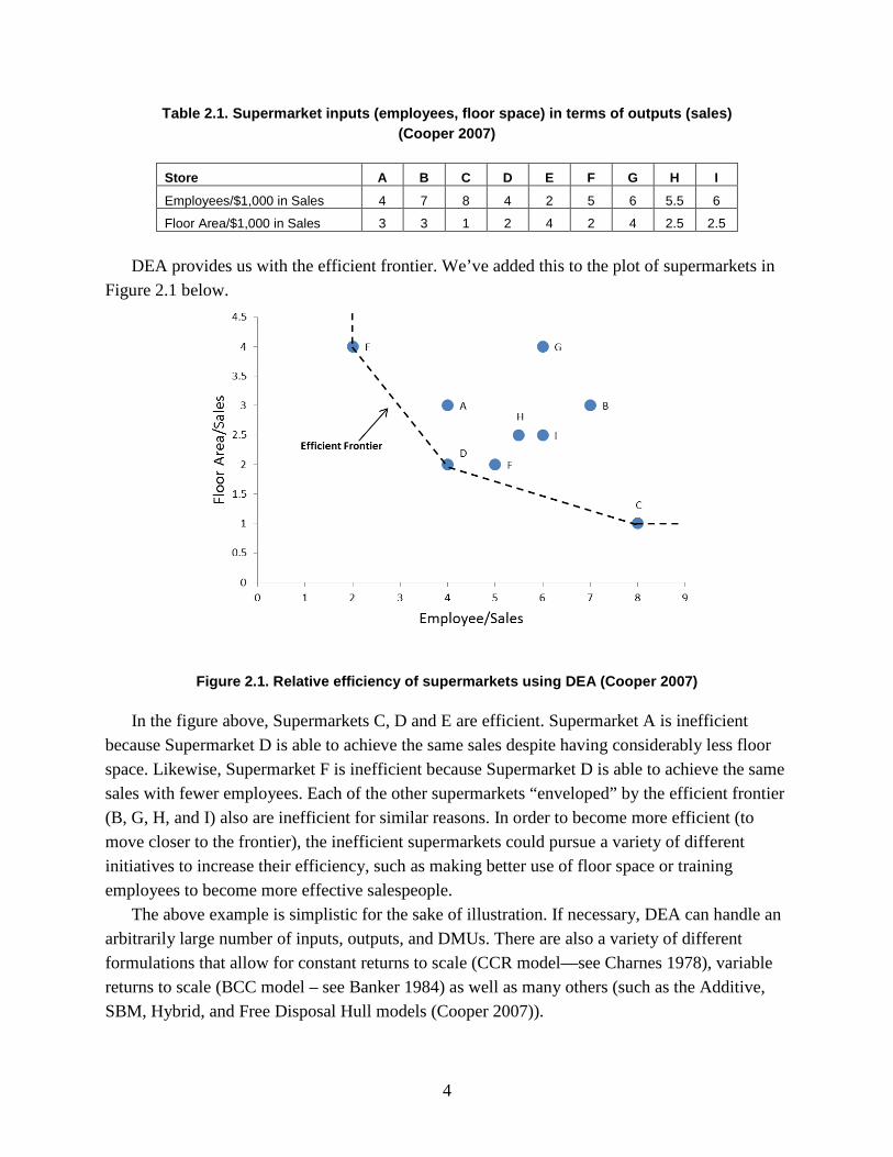
Table 2.1. Supermarket inputs (employees, floor space) in terms of outputs (sales) (Cooper 2007)

Store A B C D E F G H I

Employees/$1,000 in Sales 4 7 8 4 2 5 6 5.5 6

Floor Area/$1,000 in Sales 3 3 1 2 4 2 4 2.5 2.5 DEA provides us with the efficient frontier. We’ve added this to the plot of supermarkets in

Figure 2.1 below.

Figure 2.1. Relative efficiency of supermarkets using DEA (Cooper 2007)

In the figure above, Supermarkets C, D and E are efficient. Supermarket A is inefficient because Supermarket D is able to achieve the same sales despite having considerably less floor space. Likewise, Supermarket F is inefficient because Supermarket D is able to achieve the same sales with fewer employees. Each of the other supermarkets “enveloped” by the efficient frontier (B, G, H, and I) also are inefficient for similar reasons. In order to become more efficient (to move closer to the frontier), the inefficient supermarkets could pursue a variety of different initiatives to increase their efficiency, such as making better use of floor space or training employees to become more effective salespeople.

The above example is simplistic for the sake of illustration. If necessary, DEA can handle an arbitrarily large number of inputs, outputs, and DMUs. There are also a variety of different formulations that allow for constant returns to scale (CCR model—see Charnes 1978), variable returns to scale (BCC model – see Banker 1984) as well as many others (such as the Additive, SBM, Hybrid, and Free Disposal Hull models (Cooper 2007)).

4

Finally, further research has expanded the scope of problems to which DEA can be applied. Extensions have explored incorporating variables beyond the control of DMUs (non-discretionary variables) and categorical variables, time series comparisons (such as window analysis), as well as pairing DEA with other methods such as Stochastic Frontier Analysis (SFA) and Tobit regression to control for biases and explore causation links between variables.

2.2 Advantages and Disadvantages of DEA Technique

Advantages

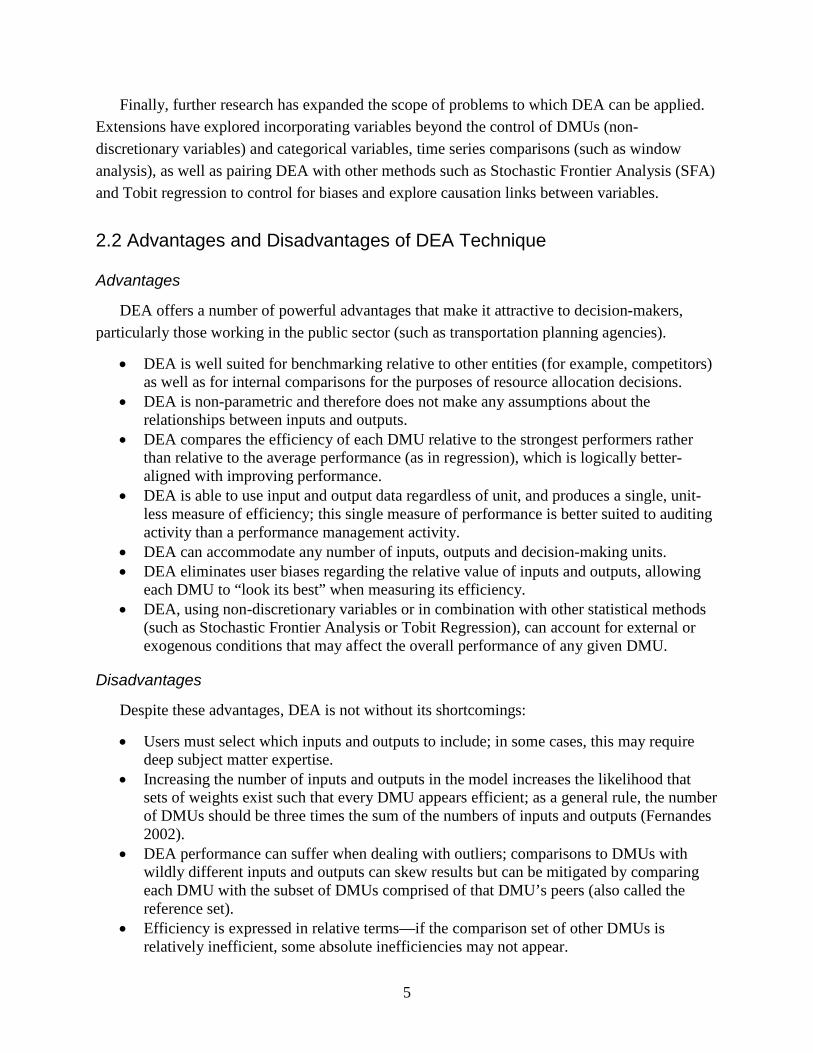
DEA offers a number of powerful advantages that make it attractive to decision-makers, particularly those working in the public sector (such as transportation planning agencies).

• DEA is well suited for benchmarking relative to other entities (for example, competitors) as well as for internal comparisons for the purposes of resource allocation decisions.

• DEA is non-parametric and therefore does not make any assumptions about the relationships between inputs and outputs.

• DEA compares the efficiency of each DMU relative to the strongest performers rather than relative to the average performance (as in regression), which is logically better-aligned with improving performance.

• DEA is able to use input and output data regardless of unit, and produces a single, unit-less measure of efficiency; this single measure of performance is better suited to auditing activity than a performance management activity.

• DEA can accommodate any number of inputs, outputs and decision-making units. • DEA eliminates user biases regarding the relative value of inputs and outputs, allowing

each DMU to “look its best” when measuring its efficiency. • DEA, using non-discretionary variables or in combination with other statistical methods

(such as Stochastic Frontier Analysis or Tobit Regression), can account for external or exogenous conditions that may affect the overall performance of any given DMU.

Disadvantages

Despite these advantages, DEA is not without its shortcomings:

• Users must select which inputs and outputs to include; in some cases, this may require deep subject matter expertise.

• Increasing the number of inputs and outputs in the model increases the likelihood that sets of weights exist such that every DMU appears efficient; as a general rule, the number of DMUs should be three times the sum of the numbers of inputs and outputs (Fernandes 2002).

• DEA performance can suffer when dealing with outliers; comparisons to DMUs with wildly different inputs and outputs can skew results but can be mitigated by comparing each DMU with the subset of DMUs comprised of that DMU’s peers (also called the reference set).

• Efficiency is expressed in relative terms—if the comparison set of other DMUs is relatively inefficient, some absolute inefficiencies may not appear.

5

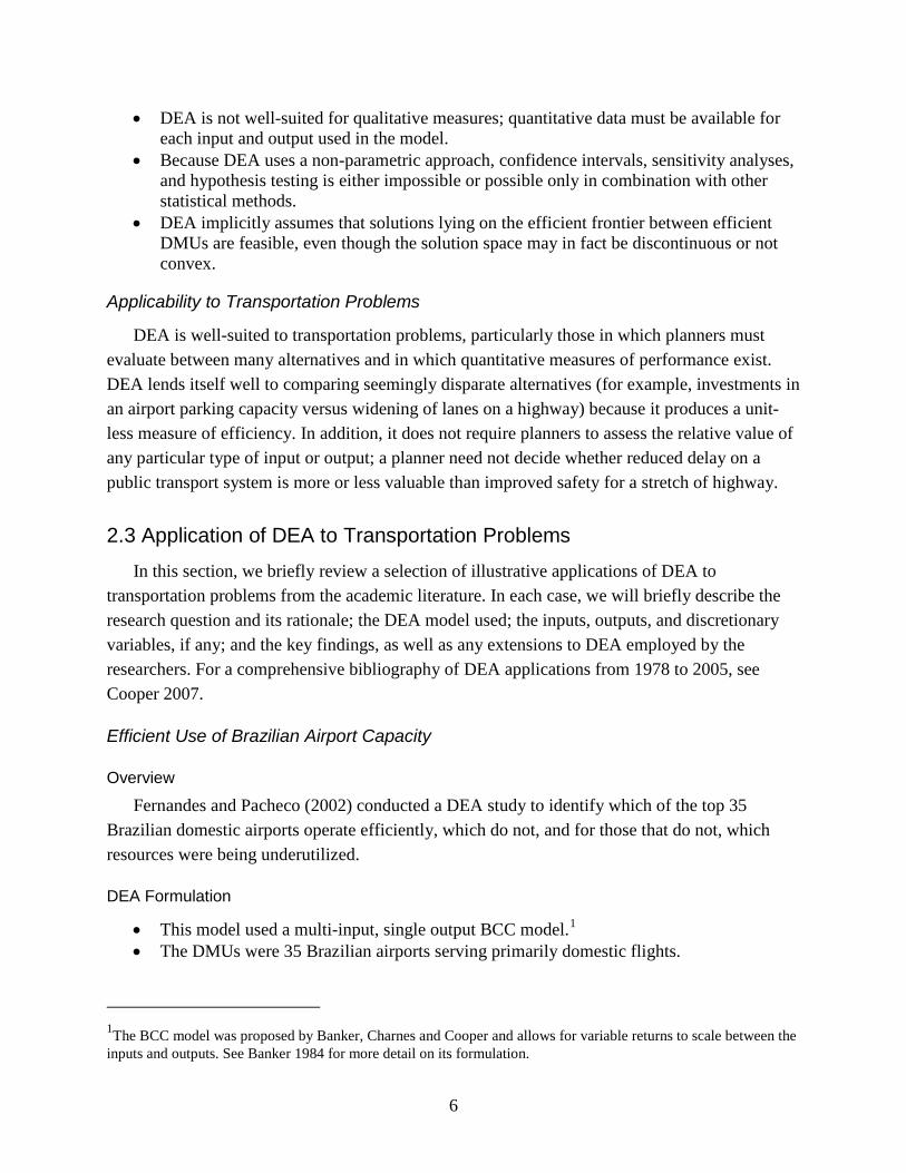
• DEA is not well-suited for qualitative measures; quantitative data must be available for each input and output used in the model.

• Because DEA uses a non-parametric approach, confidence intervals, sensitivity analyses, and hypothesis testing is either impossible or possible only in combination with other statistical methods.

• DEA implicitly assumes that solutions lying on the efficient frontier between efficient DMUs are feasible, even though the solution space may in fact be discontinuous or not convex.

Applicability to Transportation Problems

DEA is well-suited to transportation problems, particularly those in which planners must evaluate between many alternatives and in which quantitative measures of performance exist. DEA lends itself well to comparing seemingly disparate alternatives (for example, investments in an airport parking capacity versus widening of lanes on a highway) because it produces a unit-less measure of efficiency. In addition, it does not require planners to assess the relative value of any particular type of input or output; a planner need not decide whether reduced delay on a public transport system is more or less valuable than improved safety for a stretch of highway.

2.3 Application of DEA to Transportation Problems In this section, we briefly review a selection of illustrative applications of DEA to

transportation problems from the academic literature. In each case, we will briefly describe the research question and its rationale; the DEA model used; the inputs, outputs, and discretionary variables, if any; and the key findings, as well as any extensions to DEA employed by the researchers. For a comprehensive bibliography of DEA applications from 1978 to 2005, see Cooper 2007.

Efficient Use of Brazilian Airport Capacity

Overview

Fernandes and Pacheco (2002) conducted a DEA study to identify which of the top 35 Brazilian domestic airports operate efficiently, which do not, and for those that do not, which resources were being underutilized.

DEA Formulation

• This model used a multi-input, single output BCC model.1 • The DMUs were 35 Brazilian airports serving primarily domestic flights.

1The BCC model was proposed by Banker, Charnes and Cooper and allows for variable returns to scale between the inputs and outputs. See Banker 1984 for more detail on its formulation.

6

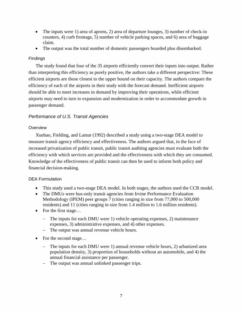
• The inputs were 1) area of aprons, 2) area of departure lounges, 3) number of check-in counters, 4) curb frontage, 5) number of vehicle parking spaces, and 6) area of baggage claim.

• The output was the total number of domestic passengers boarded plus disembarked.

Findings

The study found that four of the 35 airports efficiently convert their inputs into output. Rather than interpreting this efficiency as purely positive, the authors take a different perspective: These efficient airports are those closest to the upper bound on their capacity. The authors compare the efficiency of each of the airports in their study with the forecast demand. Inefficient airports should be able to meet increases in demand by improving their operations, while efficient airports may need to turn to expansion and modernization in order to accommodate growth in passenger demand.

Performance of U.S. Transit Agencies

Overview

Xuehao, Fielding, and Lamar (1992) described a study using a two-stage DEA model to measure transit agency efficiency and effectiveness. The authors argued that, in the face of increased privatization of public transit, public transit auditing agencies must evaluate both the efficiency with which services are provided and the effectiveness with which they are consumed. Knowledge of the effectiveness of public transit can then be used to inform both policy and financial decision-making.

DEA Formulation

• This study used a two-stage DEA model. In both stages, the authors used the CCR model. • The DMUs were bus-only transit agencies from Irvine Performance Evaluation

Methodology (IPEM) peer groups 7 (cities ranging in size from 77,000 to 500,000 residents) and 11 (cities ranging in size from 1.4 million to 1.6 million residents).

• For the first stage…

− The inputs for each DMU were 1) vehicle operating expenses, 2) maintenance expenses, 3) administrative expenses, and 4) other expenses.

− The output was annual revenue vehicle hours.

• For the second stage…

− The inputs for each DMU were 1) annual revenue vehicle hours, 2) urbanized area population density, 3) proportion of households without an automobile, and 4) the annual financial assistance per passenger.

− The output was annual unlinked passenger trips.

7

Findings

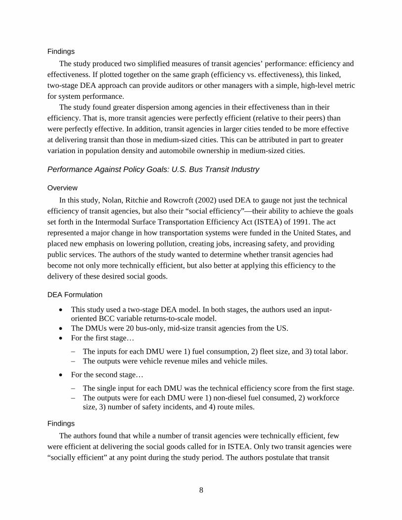
The study produced two simplified measures of transit agencies’ performance: efficiency and effectiveness. If plotted together on the same graph (efficiency vs. effectiveness), this linked, two-stage DEA approach can provide auditors or other managers with a simple, high-level metric for system performance.

The study found greater dispersion among agencies in their effectiveness than in their efficiency. That is, more transit agencies were perfectly efficient (relative to their peers) than were perfectly effective. In addition, transit agencies in larger cities tended to be more effective at delivering transit than those in medium-sized cities. This can be attributed in part to greater variation in population density and automobile ownership in medium-sized cities.

Performance Against Policy Goals: U.S. Bus Transit Industry

Overview

In this study, Nolan, Ritchie and Rowcroft (2002) used DEA to gauge not just the technical efficiency of transit agencies, but also their “social efficiency”—their ability to achieve the goals set forth in the Intermodal Surface Transportation Efficiency Act (ISTEA) of 1991. The act represented a major change in how transportation systems were funded in the United States, and placed new emphasis on lowering pollution, creating jobs, increasing safety, and providing public services. The authors of the study wanted to determine whether transit agencies had become not only more technically efficient, but also better at applying this efficiency to the delivery of these desired social goods.

DEA Formulation

• This study used a two-stage DEA model. In both stages, the authors used an input-oriented BCC variable returns-to-scale model.

• The DMUs were 20 bus-only, mid-size transit agencies from the US. • For the first stage…

− The inputs for each DMU were 1) fuel consumption, 2) fleet size, and 3) total labor. − The outputs were vehicle revenue miles and vehicle miles.

• For the second stage…

− The single input for each DMU was the technical efficiency score from the first stage. − The outputs were for each DMU were 1) non-diesel fuel consumed, 2) workforce

size, 3) number of safety incidents, and 4) route miles.

Findings

The authors found that while a number of transit agencies were technically efficient, few were efficient at delivering the social goods called for in ISTEA. Only two transit agencies were “socially efficient” at any point during the study period. The authors postulate that transit

8

agencies opted to perform to the more easily defined and measured metrics and ignored the other, harder-to-verify goals of reducing pollution, providing jobs, improving safety, and delivering public services.

The authors also compared the efficiency measures that DEA produced to another standard measure in transportation research, passenger miles per dollar operating expense (PMPDOE). The study found that DMUs with comparable efficiency scores had highly varied values for this more traditional measure, suggesting that PMPDOE may not be a reliable metric.

The Efficiency of Chicago Park-and-Ride Lots

Overview

Barnum, McNeil and Hart (2007) documented a DEA study comparing the efficiency of park-and-ride lots operated by the Chicago Transit Authority (CTA). Parking lots are a major driver of revenue for the CTA, but their construction and maintenance also are highly resource-intensive. The study was conducted to identify which lots were inefficient and to guide future decisions on lot construction, pricing, and operating policies.

DEA Formulation

• This study used a two input, two output CCR model, which assumes a constant returns-to-scale relationship between inputs and outputs.

• The DMUs were park-and-ride lots. Sixteen CTA-operated parking lots were analyzed. • The inputs for each DMU were 1) the number of parking spaces and 2) the mean daily

operating costs. • The outputs for each DMU were 1) the mean number of cars parked in the lot during the

workday and 2) the mean daily revenue.

Extensions

The researchers adopted a two-stage approach to the analysis. The first stage was the standard DEA model described above. As a second stage, the researchers undertook Stochastic Frontiers Analysis (SFA). The DEA efficiency scores were converted into “superefficiency” ratings—equivalent to the DEA efficiency score if inefficient and equal to the degree to which each DMU exceeded the efficiency threshold if efficient. These superefficiency scores were used as the dependent variable in the SFA, and “distance from central business district” and “distance from nearest freeway” were used as independent variables for each lot.

Findings

The stage one DEA found that of the 16 lots, four efficiently converted inputs into outputs. The efficiency for the remaining lots ranged from 22 percent to 98 percent. After controlling for external distance variables with SFA, only three lots were considered efficient. Those lots with low efficiency scores were flagged for further analysis.

9

The findings from this more in-depth analysis led to actionable policy recommendations for the CTA. For example, it was discovered upon closer examination that one lot with a low efficiency score was near a similarly sized lot on a very congested freeway. This led to a recommendation that prices be changed relative to the more-efficient lot to make the other lot more attractive (and therefore convince commuters to put up with the traffic to park at the more affordable lot).

In another example, one lot was staffed with CTA personnel as a security measure, while another lot was unstaffed but routinely patrolled by local police. The staffed lot had higher labor costs but still could not offer the level of security at the police-patrolled lot. It was recommended to the CTA that it pursue partnerships with local police to lower labor costs while increasing lot security.

Finally, the low efficiency scores of some underutilized lots helped the CTA identify these lots as potential targets for closing or downsizing.

Technical Efficiency of Canadian Urban Transit Systems

Overview

Boame (2004) described an application of DEA to measure the efficiency of Canadian urban transit systems from 1990 to 1998. Specifically, the author was interested in improving the resource utilization of bus transit systems by identifying the causes of changes in efficiency. The author extended the DEA approach to include a Tobit regression2 to identify the sources of change in efficiency. The author used statistical techniques to overcome some of the earlier identified shortcomings of DEA, namely the inability to accommodate random errors in input and output measurement, and the inability to use statistical inference and hypothesis testing on the efficiency values.

DEA Formulation

• This study used a multi-input, single output variable-returns to scale DEA model. • The DMUs were 30 Canadian transit systems operating conventional buses. • The inputs for each DMU were 1) fleet size, 2) liters of fuel used, and 3) total number of

paid employee hours (labor). • The output for each DMU was revenue-kilometers, a measure of the total service

supplied to fare-paying passengers.

2 Tobit regression is a statistical technique for estimating the value of a latent or unobservable variable not captured explicitly in a statistical model. Tobit regression uses linear regression to estimate this latent variable as a function of observed independent variables and a normally distributed error term. In this case, the researchers used Tobit regression to assess the impact of factors not included in the DEA model on each DMU’s performance. For more detail, see Boame 2004.

10

Extensions

As mentioned above, the author used Tobit regression to account for environmental factors that affect transit system efficiency. In particular, the study considered average road speeds as a measure of congestion, peak-to-base ratio, average fleet age, and global improvements in transit efficiency not specific to any individual transit agency.

Findings

The study yielded a number of interesting findings. The first is that, without accounting for environmental variables, ten of the transit agencies achieved 100 percent efficiency at least some of the time, and two achieved 100 percent efficiency throughout the study period. However, when correcting for the environmental variables analyzed with Tobit regression, none of the DMUs are efficient. Instead, average efficiency across all systems was about 78 percent.

The study found that most transit systems (56 percent) experience increasing returns to scale, while the remainder experience constant returns to scale (14 percent) or decreasing returns to scale (29 percent), which could have implications for decisions on which systems should receive additional funding. The study also found that transit system efficiency is significantly worsened by increases in road congestion, meaning that efforts to reduce congestion could create a positive feedback loop by enabling transit systems to operate more efficiently, leading to still-greater reductions in congestion.

Finally, the author also found that high peak demand to base demand ratios led to less efficient transit systems, and, interestingly, that fleet age had little impact on transit system efficiency.

North American Container Port Productivity

Overview

Turner, Windle and Dresner (2004) sought to determine whether growth in North American container port productivity occurred over the period of study, 1984 to 1997. The introduction of containerized shipping led to large reductions in labor costs, damage rates, and freight processing times. But, use of containers requires expensive retrofitting and modernization of port facilities and vessels. The authors were interested in determining whether container ports became more efficient and what drove these improvements. In addition, the authors were interested in determining whether it is beneficial for smaller ports to expand capacity despite the increased infrastructure costs associated with containerized shipping.

DEA Formulation

• This model used a multi-input, single output DEA model. • The DMUs were container ports. The authors treated the same container ports in different

years as different DMUs in order to track changes in efficiency over time.

11

• The inputs were 1) total terminal land dedicated to container operations, 2) total quayside container gantry cranes, and 3) total container berth length.

• The output was total 20-foot equivalent units (TEU) – a measure of the container throughput.

Extensions

The authors undertook two extensions to traditional DEA modeling. The first, mentioned above, was to allow for time-series analysis by treating each port-year as a separate DMU rather than analyzing the ports in a single snapshot.

As a second extension, the authors used Tobit regression to determine the cause of changes in port efficiency. This analysis explored whether changes in efficiency documented in the DEA study could be explained by changes in macro- and micro-level exogenous factors, such as the structure of the seaport industry, the policies of port authorities, the behavior of ocean carriers, labor, and other factors.

Findings

The study found that the productivity of container ports increased over the study period, though the rates of change varied by region and over time. In addition, the authors found that container port efficiency tended to increase with size and the degree of connectedness to rail networks. The authors suggest it may not be a good use of public funds to begin an expansion or modernization project at a small port without commitments from shippers and rail carriers to further expand the facility. Without continued expansion and rail network integration, these smaller ports may never become productive enough to recoup the initial investment.

Public transport project appraisal tool in Ireland

Overview

In this study, Caulfield, Bailey and Mullarkey (2013) investigated and identified the most efficient transport solution for the Dublin city center-airport route from a list of six alternatives that included the two existing bus routes. DEA analysis was carried out to identify the most efficient solution for the city center to the airport and to establish the reasons for efficiency.

DEA Formulation

• This study used a one input, three output CCR and BCC DEA models. • Six DMUs were used representing different alternatives considered, including two

existing bus routes, Metro North (a proposed metro route), DART spur (a new spur from the current DART network), Luas alternative (a tram line) and BRT.

• The sole input is the overall cost of implementing each transportation system that includes both the capital cost and operation and maintenance costs.

• The three outputs are number of car trips removed, patronage and travel time savings.

12

Extensions

The authors also have undertaken slack analysis to observe how far some options are from an efficient solution and have further undertaken sensitivity analysis to evaluate the robustness of the results obtained. The sensitivity analysis is performed by including and excluding one or more variables in the model to observe the resulting differences in the DEA efficiencies from a base model. On the basis of the DEA efficiencies obtained from the base model and the sensitive analysis, each alternative was classified into five different categories ranging from robustly efficient to distinctly inefficient.

Findings

The study yielded a number of interesting findings. The BRT and DART spur are the two most efficient solutions, while the Luas alternative and Metro North appear to be ineffective due to their scale sizes, although considerable scope for improvement in efficiency can be achieved by downsizing their operations. In addition, the Metro North is the least efficient solution predominantly due to excessive cost. Sensitivity analysis indicated the BRT airport scheme is the only alternative that is robustly efficient; the DART spur is marginally efficient; and the rest of the alternatives are distinctly inefficient.

Performance analysis of European Airports

Overview

In this study Suzuki et al., (2012) undertook a comparative analysis of the efficiency of 19 European airports using two different formulations of BCC DEA models. Two different formulations were specified to address the methodological and substantive weaknesses in the BCC DEA models.

DEA Formulation

• Nineteen DMUs were used representing a set of European airports. • This study used four inputs and two outputs. All the inputs and outputs relate to the year

2003 for which the analysis was undertaken. • The inputs are the number of runways, terminal space (m2), the number of gates and the

number of employees. An additional input, the shopping area, was used to carry out sensitivity analysis with and without commercial activities.

• The two outputs are the number of passengers and aircraft movements.

Extensions

The first formulation (distance friction minimization, BCC-DFM) was developed with a view toward generating a more appropriate efficient projection model than in the standard BCC DEA model used widely in airport efficiency studies. The second formulation (BCC-DFM-FF) is a

13

further extension of the first that incorporates fixed factors as exogenous inputs or outputs in a BCC-DFM model.

Findings

Like the Ireland study, this study yielded multiple interesting findings. Commercial activities were found to be very important for the airports in financial terms. Inclusion of the shopping area in the terminal as an input in the model has relatively little influence on the relative efficiency levels. Results also suggested that to reach an efficient frontier, the reduction in inputs required is far less in the new formulation than in the standard BCC DEA model.

14

3. Review of Conjoint Analysis in Practice

3.1 Overview Conjoint analysis (CA) refers to a set of techniques that can be used to determine the relative

weights that individuals implicitly apply when they make choices. The method assumes that the features3 of a product, service or (for this application) program or project can be traded off against each other and that weights on each of those features can be calculated from properly designed elicitation exercises. The values of the calculated weights for each of the features can then be used to determine the relative preferences among project or program alternatives that consist of different combinations of features.4

Conjoint analysis (CA) is extensively used in the area of market research, but in the last four decades, conjoint analysis also has become a commonly-employed tool in a number of other fields including transportation, health care, telecommunications, banking, and management of natural resources. Over that period, CA also has come to encompass a broad array of approaches, distinguished both by the elicitation methods and by the statistical techniques that are used to derive feature weights. All of the methods use specially designed survey elements to elicit information about feature trade-offs, and all derive weights of some form for each of the features.

Depending on the specific approach used, the weights could be calculated to indicate the ordering and relative strength of preferences among different project alternatives for a given individual or for a group of individuals. The weights can be estimated using any of several different techniques, depending in part on the elicitation method. In some cases, the conjoint exercises can be structured so that a simple count of responses to the different exercises can be used to estimate weights. However, other statistical estimation approaches most often are used. These approaches assume that the preference for, or the “utility” of a given project or program, is a function of the features of that project or program. However, it is also recognized that random factors can enter an individual’s consideration of a given project, representing features that are not explicitly included in the conjoint exercises or general variability in the way that an individual responds to different alternatives. It is assumed that individuals make selections in the exercises that represent alternatives that maximize their utility values, including this random component.

3 Conjoint analysis literature typically uses the term “attribute” to refer to the elements that are traded-off but the text here will use the term “feature” interchangeably. 4 Although conjoint analysis can equivalently be applied to evaluation of products, services, individual projects or programs consisting of several projects, the text that follows will refer to “projects” for consistency with the applications of interest here.

15

Different assumptions about the distributions of the random components lead to different forms of mathematical models in which the feature weights are embedded. The most commonly-used among these is the multinomial logit model, which has been used to represent a wide array of situations in which choices are made among a discrete set of alternatives. One of the earliest applications of this model was to determine the implicit weights that decision-makers in a transportation agency used in selecting among different highway project alternatives (McFadden, 1976). In that case, the feature weights were estimated using data on actual choices that the agency made among alternatives that each consisted of different combinations of features. In most cases, however, there is insufficient information on past choices and, hence, conjoint-type survey elicitation methods are used to supply the information that is needed for this type of weight calculation.

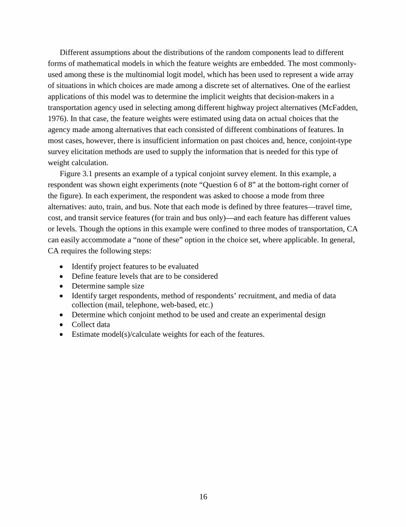
Figure 3.1 presents an example of a typical conjoint survey element. In this example, a respondent was shown eight experiments (note “Question 6 of 8” at the bottom-right corner of the figure). In each experiment, the respondent was asked to choose a mode from three alternatives: auto, train, and bus. Note that each mode is defined by three features—travel time, cost, and transit service features (for train and bus only)—and each feature has different values or levels. Though the options in this example were confined to three modes of transportation, CA can easily accommodate a “none of these” option in the choice set, where applicable. In general, CA requires the following steps:

• Identify project features to be evaluated • Define feature levels that are to be considered • Determine sample size • Identify target respondents, method of respondents’ recruitment, and media of data

collection (mail, telephone, web-based, etc.) • Determine which conjoint method to be used and create an experimental design • Collect data • Estimate model(s)/calculate weights for each of the features.

16

Figure 3.1. Example of a Conjoint Based Choice (CBC) Experiment

The numbers of features, levels, and experiments presented to a respondent affect the sample’s required size. In general, calculating weights for more features, each with more levels, requires a larger sample size. Similarly, a smaller sample size is likely to entail more experiments per respondents.

3.2 Advantages and Disadvantages of CA Technique

Advantages

CA produces weights for the features that comprise a set of projects or programs, and those weights then can be used to prioritize alternative projects or programs.

• The feature weights that are calculated using CA directly reflect the preferences of the decision-makers or other stakeholders who complete the survey exercises.

• CA works especially well for calculating weights for up to about 10 features. • Features can be described using qualitative, categorical or continuous variables. • CA is commonly employed in many fields, and substantial literature is available

describing methods and applications.

17

• Widely available commercial and open-source software exists to support CA surveys and statistical modeling.

Disadvantages

As with any method, CA has limitations:

• Special approaches are needed to deal with applications involving a large numbers of features (10 or more).

• The method requires direct input from decision-makers and/or other stakeholders and the weights are a function of their responses. So they may need to be updated to reflect changes in these groups or changing societal preferences.

Applicability to Transportation Problems

Conjoint analysis can be used to evaluate a wide range of transportation problems. For example, transportation projects that states or major metropolitan regions typically consider can vary widely in the types of benefits they provide and in the scales of those benefits. In such cases, simply choosing projects that provide the greatest net economic benefits may not result in a mix of projects that most effectively accomplishes an agency’s goals and objectives. Conjoint analysis provides a framework for project prioritization that incorporates decision-makers’ and stakeholders’ preferences on multiple goals that could be measured either quantitatively or qualitatively, improving transparency, equity, and collaboration of the project prioritization process.

In the next sections, selected examples of applications of conjoint analysis in transportation investment prioritization are discussed. Additional examples of application of conjoint analysis in long-term investment decisions in housing and transportation, natural resource management, and health care prioritization are provided in Appendix C. While the examples below present applications of a number of conjoint and conjoint-related methods—such as stated preference (SP) survey, analytical hierarchy process (AHP), multi attribute utility theory (MAUT), and discrete choice modeling (DCM)—all of them follow the same process: elicitation of feature trade-offs followed by estimation of weights to be used for studies/projects evaluation.5

3.3 Application of CA for Prioritizing Transport Infrastructure Investments Prioritizing competing transport infrastructure investments always has been a challenge as

policymakers deal with establishing a credible, transparent process for selecting the most appropriate projects under limited resources. The most appropriate evaluation methods for transport projects are either based on cost-benefit analysis (such as Damarat and Roy, 2009) or Multi-criteria techniques (Tsamboulas, 2007) and in some cases combinations of both are used

5 Detailed descriptions of SP, AHP, MAUT, and DCM are beyond the scope of this report.

18

(such as Gühnemanna et al., 2012). The strengths of cost–benefit analysis are that it constitutes a homogeneous frame of reference for evaluating investment projects. However, such as it is applied currently, the highly technical character and the formalism of CBA is a disadvantage that makes the method difficult to integrate into public debate (Damarat and Roy, 2009). Multi-Criteria analysis facilitates a stronger alignment with espoused transport policy by allowing impacts that cannot be expressed on a monetary scale or easily be quantified, but which policymakers recognize as important, such as distributional impacts, environmental effects or the achievement of strategic policy goals, to be formally included in an appraisal (Gühnemanna et al., 2012). Although different methods for incorporating the multi-criteria analysis have been used, we list three studies in which CA-based approaches have been used for prioritization problems.

Puget Sound Regional Council Transportation Project Prioritization

One of the most recent and relevant applications of CA in transportation was conducted for the Puget Sound Regional Council. For this study, a CA-based approach to project prioritization was developed to support stakeholder-based weighting of multiple goals and, for each goal, multiple measures. The approach uses the analytic hierarchy approach to develop weights for each goal and a conjoint-based method to estimate stakeholder weights for each measure.

The approach was applied as part of the Puget Sound Regional Council’s Transportation 2040 process and achieves the goals in VISION 2040, the long-range land use plan. Weighting exercises were conducted with two stakeholder groups and the results were applied to a set of proposed ferry, rail, highway and local road projects.

To fully characterize the different projects, a total of 17 project features (“measures”) were to be included in the analysis. This is a larger number than can be easily included in a CA study and so this study used a complementary method, Analytic Hierarchy Process (AHP; see Saaty, 1980 for a description of this method) to develop weights for five general goals and then CA to develop importance weights for the features associated with those goals. Figure 3.2 below shows the features (measures) and goals (outcomes) that were to be included in the prioritization process.

19

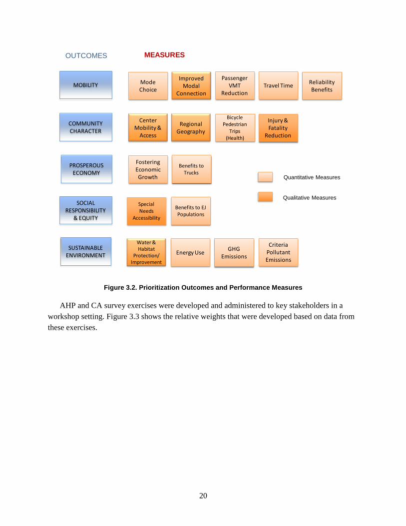
Figure 3.2. Prioritization Outcomes and Performance Measures

AHP and CA survey exercises were developed and administered to key stakeholders in a workshop setting. Figure 3.3 shows the relative weights that were developed based on data from these exercises.

OUTCOMES

MOBILITY

COMMUNITY CHARACTER

PROSPEROUS ECONOMY

SOCIAL RESPONSIBILITY

& EQUITY

SUSTAINABLE ENVIRONMENT

Mode Choice

MEASURES

Improved Modal

Connection

Passenger VMT

ReductionTravel Time Reliability

Benefits

Center Mobility &

Access

Bicycle Pedestrian

Trips (Health)

Injury & Fatality

Reduction

Fostering Economic Growth

Benefits to Trucks

Special Needs

Accessibility

Benefits to EJ Populations

Water & Habitat

Protection/ Improvement

Energy Use GHG Emissions

Criteria Pollutant Emissions

Regional Geography

Qualitative Measures

Quantitative Measures

20

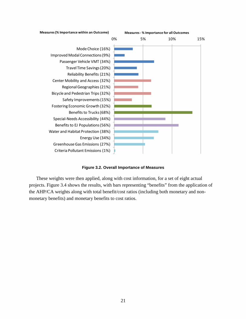
Figure 3.2. Overall Importance of Measures

These weights were then applied, along with cost information, for a set of eight actual projects. Figure 3.4 shows the results, with bars representing “benefits” from the application of the AHP/CA weights along with total benefit/cost ratios (including both monetary and non-monetary benefits) and monetary benefits to cost ratios.

Mode Choice (16%)Improved Modal Connections (9%)

Passenger Vehicle VMT (34%)Travel Time Savings (20%)Reliability Benefits (21%)

Center Mobility and Access (32%)Regional Geographies (21%)

Bicycle and Pedestrian Trips (32%)Safety Improvements (15%)

Fostering Economic Growth (32%)Benefits to Trucks (68%)

Special-Needs Accessibility (44%)Benefits to EJ Populations (56%)

Water and Habitat Protection (38%)Energy Use (34%)

Greenhouse Gas Emissions (27%)Criteria Pollutant Emissions (1%)

0% 5% 10% 15%Measures (% Importance within an Outcome) Measures - % Importance for all Outcomes

21

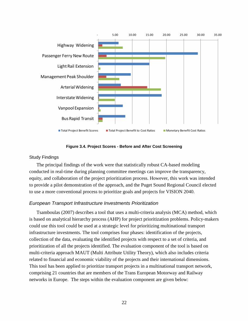
Figure 3.4. Project Scores - Before and After Cost Screening

Study Findings

The principal findings of the work were that statistically robust CA-based modeling conducted in real-time during planning committee meetings can improve the transparency, equity, and collaboration of the project prioritization process. However, this work was intended to provide a pilot demonstration of the approach, and the Puget Sound Regional Council elected to use a more conventional process to prioritize goals and projects for VISION 2040.

European Transport Infrastructure Investments Prioritization

Tsamboulas (2007) describes a tool that uses a multi-criteria analysis (MCA) method, which is based on analytical hierarchy process (AHP) for project prioritization problems. Policy-makers could use this tool could be used at a strategic level for prioritizing multinational transport infrastructure investments. The tool comprises four phases: identification of the projects, collection of the data, evaluating the identified projects with respect to a set of criteria, and prioritization of all the projects identified. The evaluation component of the tool is based on multi-criteria approach MAUT (Multi Attribute Utility Theory), which also includes criteria related to financial and economic viability of the projects and their international dimensions. This tool has been applied to prioritize transport projects in a multinational transport network, comprising 21 countries that are members of the Trans European Motorway and Railway networks in Europe. The steps within the evaluation component are given below:

- 5.00 10.00 15.00 20.00 25.00 30.00 35.00

Highway Widening

Passenger Ferry New Route

Light Rail Extension

Management Peak Shoulder

Arterial Widening

Interstate Widening

Vanpool Expansion

Bus Rapid Transit

Total Project Benefit Scores Total Project Benefit to Cost Ratios Monetary Benefit Cost Ratios

22

Definition of criteria:

In order to be as exhaustive as possible and to define the objectives of evaluating properly, a two-step consultation process was used to select the criteria that reflected the preferences of the stakeholders. A total of 15 criteria were identified and were organized into three clusters (five criteria in each cluster) reflecting the socio-economic returns on investment, functionality and coherency of the transport network and strategic/political concerns of the involved national and international authorities.

Criteria values per project:

The criteria for each project are measured either by direct classifying the available data on measureable characteristics or by “quality attributes” provided by the expert judgment from the national authorities involved. To arrive at various criterion scores, they were converted into one common measurement unit and the criteria value calculation was based on direct scoring on an artificial scale.

Criteria Weighting:

The weights for each criterion were based on the analytical hierarchy process (AHP) in which a panel of experts, including the stakeholder steering group and experts from international and national organization and institutes, provided a pairwise comparison of criteria on a nine-point scale, in which 1 implies that the criteria are equally important and 9 implies that the base criterion against which other criteria are compared is overwhelmingly more important than the other factor.

Derivation of the total score per project:

The total score for each project in a given region is the sum product of the criteria values and the weights assigned to the respective criteria across all the criteria. Further, the overall score per project is given as the sum product of the total score for each project in a given region and the spatial weight for the project in that region across all the regions included in that project. Spatial weights are derived across each region depending upon the fraction of length/catchment area of a given project in a given region to the overall length/catchment of the project.

Depending upon the total score per project, four prioritization categories have been established reflecting the timeframe for implementing the projects. For example, category 1 projects reflect the need to implement the projects immediately, and category 4 projects need to be implemented in a longer term.

Ivanovic et al. (2013) uses a similar tool (ANP-based MCA) to select different alternatives that can be used for street reconstruction into pedestrian area in one city in the southeastern Balkans. Street network alternatives were considered and evaluated based on five criteria that were further defined by two sub-criteria within each of them. The weights to each criterion were based on a two-part survey administered to the stakeholders (traffic experts, members of local

23

government and five residents). The first part of the survey collected the stakeholder’s evaluation of the influence each criteria has on the proposed alternative in a three-point impact scale—low, medium and high. In the second survey, the stakeholders provided a pairwise comparison of criteria on a 10-point scale. The weights to the each criterion then were obtained using AHP.

CA/SP Methods as an Alternative to Analytical Hierarchy Process (AHP) for Obtaining Criteria Weights

The above studies demonstrate the use of multi-criteria analysis as a decision-making tool for prioritizing competing transport investments. The critical component of the process is the evaluation framework in which the criteria are defined and weighted and the projects are evaluated against these criteria with the established weights. This method inherently relies on experts/stakeholders providing a pairwise comparison. AHP methods have been used for establishing the weights as they provide rapid and reliable weights—rapid in expressing the short time necessary for its application and reliable in minimizing the subjectivity of weights’ values (Tsamboulas, 2007).

CA-based methods also could be used for establishing the criteria weights, though we have been not able to find comparison studies within the transport sector that compare both the AHP and CA methods within the MCA framework. However, studies within the healthcare sector (for example, Ijzerman et al., 2012) compare the AHP and CA methods in assessing treatment alternatives for stroke rehabilitation. This study demonstrated that the AHP and CA have equal predictive and convergent validity although differences exist between AHP and CA in predicting the preferences; the methods seemed to result in a different rank order of the treatments. The advantage of CA over AHP is that it offers more realistic choices and can be easily administered for large groups of people. Consequently, the results can be generalized to a wider population. Whereas, the advantage of AHP over CA is that it is easier to use and quite flexible for a number of healthcare decisions. It concludes that the decision context and practical considerations such as ease of application should determine which method to use. MCA using CA-based methods are advantageous, especially for large transport projects/investments which generate a lot of public interest and debate and when a need arises to consider the preferences of the wider public in transport investment decisionmaking.

24

4. Review of Fair Division Analysis in Practice

4.1 Overview Fair division analysis (FDA) involves dividing a set of (sometimes indivisible) goods or

services between two or more agents such that each agent receives a fair allocation. There are many different fair division methods for dividing goods and services. Many of these are algorithm-based. That is, subject to a set of rules, the agents select a strategy that will provide them with a “fair” allocation. Other fair division methods are optimization-based. These methods use an objective function to define “fair” and the allocation is optimized to maximize “fairness.” All methods differ in their level of “fairness,” defined by four characteristics. That is, in fair division theory, the division is said to be fair if it has the following properties:

• Envy-freeness. If no agent is willing to trade their portion for another agent’s portion, the division is said to be “free of envy.”

• Proportionality. Given n agents, if each agent received at least 1/n of the total value of the goods or services, the division is said to be “proportional.”

• Equitability. Given utilities assigned to the goods or service, if all agents’ individual utility with their allocation of goods or services is equal, the division is said to be “equitable.”

• (Pareto) Efficiency. If there is no other allocation that is better for some agent without being worse for some other agent, the division is said to be “efficient” (Brams 2003).

Fair division theory was devised by a set of mathematicians in the 1940s (Knaster and Steinhaus 1946, Steinhaus, 1948, 1949). These theories were revived for the more modern approach to fair division by Brams and Taylor (1996, 1999) and Robertson and Webb (1998). These authors proposed a number of different rules-based procedures for dividing both divisible (for example, land) and indivisible (such as non-monetary inheritance) goods. The most classic fair division method is the “Divide and Choose” method commonly applied to cake-cutting problems. How can a mother get two children to divide a piece of cake fairly? One child cuts the cake and the other chooses between the two pieces. The Divide and Choose method becomes more complex to conduct, and achieving “fairness” becomes more difficult, as the number of agents increase. Two points of the Divide and Choose method make it interesting: (1) the set of goods or services under consideration is not necessarily homogenous and (2) the agents may have different preferences for the heterogeneous items. However, the method is impractical for dividing indivisible goods.

A number of other rules-based fair division methods have been proposed and applied since the 1940s. One that is equally simple is the Strict Alternation or Balanced Alternation method (Brams 2003). In Strict Alternation, the agents simply take turns choosing an item from the collection. However, the ordering of turns may cause the method to be “unfair.” Instead,

25

Balanced Alternation alternates the ordering of turns for each round. Thus, in a game of three agents, if a specific agent went first the first round, they would go third in the second round, first in the third round and so on until all items were divided. Another rules-based method, known as Adjusted Winner, uses a form of artificial currency to impose value on a collection of items (Brams 2003). For instance, two agents each distribute a total of 100 points across a set of items to be divided, depending on their preferences for each item. Each item is initially allocated to its highest bidder. The allocation is then adjusted by transferring items between agents until the point totals of each individual agent are equal. In Knaster’s procedure of sealed bids (Knaster and Steinhaus 1946), the items are given a monetary value and, based on the sum of those values, a fair allocation value is determined. As with Adjusted Winner, each item is allocated to the agent who values it most. However, instead of a transfer of these items to reach an envy-free solution, the agent with a greater point total makes monetary payments to compensate the agent with the point deficit.

Optimization-based methods may require computing power to attain “fair” solutions. The complexity of these methods partially depends on the number of agents and the number of goods. For example, allocating 10 goods to five agents will result in 510 = 9.8 x 106 allocations and 210 = 1024 bundles (solution) for each agent to consider. Complexity can also be mitigated by choosing the proper objective function to search the space of alternative bundles for the best solution. The objective function compactly represents preferences over the large number of bundles. For example, a generalized optimization-based method is the Rawlsian maximin criteria (Rawls 1999). Given a ranking by each agent for all items in a collection, the objective function of this criteria finds the division that maximizes the minimum rank of items that agents receive, making the worst-off agent as well off as possible.

Fair division theory has been applied to many hypothetical problems in the economics and game theory literature, mainly for the purposes of finding axioms that characterize fairness in terms of the four characteristics presented previously. These applications attempt to establish the existence (or nonexistence) of an allocation to a hypothetical problem that satisfies a number of “fairness” properties. Applications of fair division analysis in real-world problems are less common. Applications of rules-based methods include those to divide an inheritance, as well as other indivisible items. Optimization-based methods are often used in environmental problems that require the coupling of an objective function with a model simulating physical processes, such as water distribution. A few studies from each type of method are summarized in more detail in the following sections.

26

4.2 Advantages and Disadvantages of FDA Technique

Advantages

Each approach for fair division analysis is suitable for different types of problems and may or may not achieve the properties of envy-freeness, proportionality, efficiency and equitability. However, some general advantages to fair division analysis methods include:

• The ability to find solutions, using the rules-based fair division analyses, without the use of numerical computation tools.

• The simplicity of the rules-based FDA methods allow for it to be implemented without any special expertise or training.

• The ability to determine a “fair” allocation of indivisible goods and services, in addition to divisible goods.

Disadvantages

As with any method, FDA has limitations:

• The customizable nature of fair division rules and its objective function may impose a level of unchecked subjectivity to an allocation solution.

• FDA remains relatively unemployed in real-world applications, and the literature describing these applications are obscure.

• Optimization-based methods do not appear to be explicitly supported by existing software—rather, a programmer must develop code to perform such optimizations.

• Optimization-based methods may require significant computing power.

Applicability to Transportation Problems

FDA provides a means of incorporating the opinions of multiple stakeholders into the allocation decision. Thus, the technique may be especially helpful when the resource allocation will affect many stakeholders and transportation decision-makers want to ensure that the final allocation is “fair” for all of the stakeholder groups involved. Additionally, the technique allows for the allocation of resources without the use of numerical computational tools or any special expertise on the part of the analyst. Therefore, if a state DOT does not have resources to invest in statistical tools or expertise, using FDA allows for a method for resource allocation that does not require this investment.

4.3 Application of FDA in Transportation Problems This section provides an example of the application of FDA in transportation problems.

Applications of FDA to environmental problems and to allocating indivisible goods are provided in Appendix C.

27

Texas Department of Transportation

In this study, fair division analysis was used to design a model that can allocate transportation funds to specific projects within 25 districts across the state of Texas (Gurrola and Taboada 2011). The study involved incorporating a model designed to solve high complexity combinatorial optimization problems, incorporating fair division concepts or envy-freeness, efficiency and equitability.

Objective Function/Decision Criteria or Rules:

A fair division problem was modeled based on the following rules:

• Given the:

− Number of districts, − Number of funding categories − Cost of projects in each district

• Maximize the utility, defined as the sum of the cost of the funded projects within each district divided by the cost of the projects expected to be funded.

• Minimize the “envy” of each district, defined as the sum of the differences in utility between a specific district and all other districts.

Type of FDA methods used:

• Optimization-based

Findings:

This model was run for a case study with six districts and five funding categories with differing funding levels. It generated a search space of 500 solutions, with the minimum “sum of envy” being the solution of interest to the authors.

Implementation of study findings:

The study provided a means of allocating funds proportional to the size of the districts. The work could be incorporated into a state DOT allocation program as a methodology that can search for equitable allocations that minimize envy.

28

5. Preparation of a hypothetical plan

5.1 Introduction One of the key components of the current research is to define a plan that can be employed as

an evaluation and prioritization framework for Statewide Transportation Improvement Program (STIP) projects. The plan, which the NCHRP staffs and panel members approved, includes both qualitative and quantitative evaluation criteria to simulate settings faced by DOT staff in real life. During the plan’s development, the research team reached out and interviewed two groups of users: (1) professionals who are considered by their peers expert in the fields of Data Envelopment, Fair Division, and Conjoint Analysis, and (2) DOT practitioners.

To ensure consistency and uniformity in responses, for each user group a set of questions were identified before any interview was conducted (See Appendix A for the guide for interviewers.). The purpose of these interviews was to use the experts’ input as a guidance to the plan development and to use the practitioners’ input to develop a hypothetical case study. In total, four experts were interviewed: two U.S. academics, each with more than 30 years of experience; a U.S. practitioner with more than 10 years of academic experience and more than 30 years of related consulting experience in the United States and a European academic with more than 25 years of experience and extensive publications.

The research team carefully selected this group of experts who represent both academia and practice and have experience in the United States as well as Europe to obtain unique perspectives and valuable information during the development stage of the plan. Similarly, Colorado, Kansas, Michigan, Minnesota, New Mexico, North Carolina, Oregon, Washington, and Wyoming DOTs were selected for interviews to obtain important insights into DOTs who represent a wide range of state sizes and who already have somewhat advanced project prioritization processes in place. In the next section, the set of evaluation criteria included in the plan are discussed.

5.2 Evaluation Criteria The development of the plan involved identifying a set of project/program evaluation criteria that are meaningful, easy to understand, relatively common across the DOTs, and have data requirements that are reasonably easy to collect. The research team also understands that quite often, the DOTs may select projects and programs that are likely to make noticeable contributions toward achieving agencies’ certain goals and objectives. Thus, it is important to define an evaluation framework that includes agencies’ goals. In addition, project selection committees may include members who represent a wide range of interests and perspectives such as public transport, freight, and sustainable community an effective evaluation framework must

29

incorporate their interests. Further, very few alternative projects are evaluated based solely on qualitative benefits. Therefore, it is imperative that evaluation criteria should include both qualitative and quantitative measures to adequately represent policies of interest. Table 5.1 presents project/program evaluation and prioritization criteria proposed in the current study. As may be observed from the table, the framework includes 24 criteria/performance measures that fall under the following eight goals:

• Promote/support economic growth • Improve mobility • Support a sustainable environment • Safety • Promote social responsibility • Create/support an inclusive community • Are consistent with local/regional/state plans • Provide a return on investment.

30

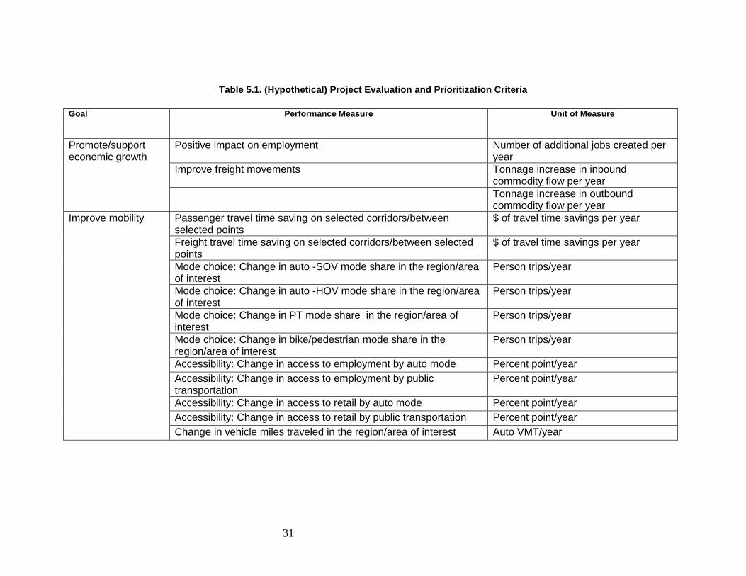
Table 5.1. (Hypothetical) Project Evaluation and Prioritization Criteria

Goal Performance Measure Unit of Measure

Promote/support economic growth

Positive impact on employment Number of additional jobs created per year

Improve freight movements Tonnage increase in inbound commodity flow per year

Tonnage increase in outbound commodity flow per year

Improve mobility Passenger travel time saving on selected corridors/between selected points

$ of travel time savings per year

Freight travel time saving on selected corridors/between selected points

$ of travel time savings per year

Mode choice: Change in auto -SOV mode share in the region/area of interest

Person trips/year

Mode choice: Change in auto -HOV mode share in the region/area of interest

Person trips/year

Mode choice: Change in PT mode share in the region/area of interest

Person trips/year

Mode choice: Change in bike/pedestrian mode share in the region/area of interest

Person trips/year

Accessibility: Change in access to employment by auto mode Percent point/year Accessibility: Change in access to employment by public transportation

Percent point/year

Accessibility: Change in access to retail by auto mode Percent point/year Accessibility: Change in access to retail by public transportation Percent point/year Change in vehicle miles traveled in the region/area of interest Auto VMT/year

31

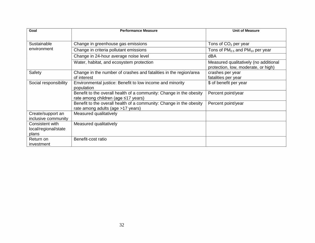
Goal Performance Measure Unit of Measure

Sustainable environment

Change in greenhouse gas emissions Tons of CO2 per year Change in criteria pollutant emissions Tons of PM2.5 and PM10 per year Change in 24-hour average noise level dBA Water, habitat, and ecosystem protection Measured qualitatively (no additional

protection, low, moderate, or high) Safety Change in the number of crashes and fatalities in the region/area

of interest crashes per year fatalities per year

Social responsibility Environmental justice: Benefit to low income and minority population

$ of benefit per year

Benefit to the overall health of a community: Change in the obesity rate among children (age ≤17 years)

Percent point/year

Benefit to the overall health of a community: Change in the obesity rate among adults (age >17 years)

Percent point/year

Create/support an inclusive community

Measured qualitatively

Consistent with local/regional/state plans

Measured qualitatively

Return on investment

Benefit-cost ratio

32

While these goals do not correspond to objectives of any specific agency, the research team identified the above goals to include a broad range of criteria that reflect traditional measures as well as “soft” measures that DOTs across the country increasingly are employing. Also, the selected goals closely follow the MAP-21 national goals6 and will help states to transition towards a performance-based program, where necessary.

In this exercise, feedback from the experts and the DOT staffs provided valuable information. For example, feedback from the experts allowed us to identify the space of problems such as limitations with each technique in terms of the maximum number of projects/programs and criteria that can be optimized. Feedback from the DOT staff underscored the importance of specifying a framework that includes a wide range of policies of interest and contains both qualitative and quantitative measures. The last column in the table lists units that may be utilized to quantify each evaluation criteria. Some of the criteria may be measured in monetary value; others provide non-monetary impact of a particular alternative. The application of techniques, such as Conjoint Analysis, recognizes this and is capable of combining monetary values with other quantitative and qualitative values.

The project/program evaluation and prioritization criteria discussed above are applied to the DEA and CA techniques. As explained in the next section, FDA does not require (or accommodate) the use of attributes to describe a project. Instead, the projects are evaluated holistically. That is, the evaluation will be based on project/program level preferences and a “fairness” algorithm.

5.3 Application of Each Technique: Selected Methods

Data Envelopment Analysis

A variety of alternative methods are available for formulating DEA analysis. One such approach, the variable returns to scale model (also known as the BCC model), is well suited to transportation planning problems. The variable returns to scale model allows for non-linear relationships between inputs and outputs. The analyst can select from either an input-oriented or output-oriented model: If the analysis is focused on reducing inputs (such as lowering costs), an input-oriented model is best; if the analysis instead is focused on producing more outputs (such as increasing passenger-miles), an output-oriented model is best. The analyst also can choose to include categorical variables and non-discretionary variables to capture environmental conditions that cannot be quantitatively measured or are beyond the control of managers of the DMUs.

6 The Moving Ahead for Progress in the 21st Century Act (MAP-21) established the following national performance goals for the Federal Highway Programs: (1) safety, (2) infrastructure condition, (3) congestion reduction, (4) system reliability, (5) freight movement and economic vitality, (6) environmental sustainability, and (7) reduced project delivery delays.

33

Conjoint Analysis

Conjoint analysis encompasses a wide range of specific methods, each of which has its own domain of appropriate applications. Generally speaking, these methods all involve a structured survey element that has respondents trade off different levels of each of the attributes being tested. The data from these trade-off exercises then can be used to develop individual-level or aggregate (average) preference weights for each of the attribute levels. The weights can be estimated using any of several different methods. For the current study, average weights were estimated using a multinomial logit model (MNL). MNL models are widely used in transportation to predict the behavior of interest of a group of individuals/decision-makers. The model can be easily estimated using a variety of open-source software packages. The estimated weights can be applied in a straightforward manner to calculate a single “score” for each project, which then can be used to determine the optimal set of projects in a program. The results of the project scoring can be graphically displayed in ways that make that information and its implications easily understandable.

Fair Division Analysis

The fair division methods provide a holistic evaluation of the goods or services that are to be allocated. That is, the decision-makers or stakeholders surveyed to determine the resource allocation are asked to state their preferences for each good or service, rather than evaluating specific attributes of the good or service.

In the current study, we employed a method that was previously applied in Kiryluk 2013. The method involves eliciting the preferences of multiple stakeholder groups that each has different motivations and objectives surrounding the program/project prioritization. One group must be the beneficiaries of the programs. Preferences are provided at the program/project level, as opposed to at the attribute level, which is the norm for DEA and CA techniques. Upper bounds and lower bounds are chosen for budget allocations of each program based on a set of objective criteria, such as the size of the targeted group of beneficiaries of that program. A fairness algorithm then is established using FDA by determining the order of payments, in which programs are funded first that have the largest difference between the average stakeholders’ preference and the beneficiaries’ preference. Finally, a payoff table developed using the beneficiaries’ preferences determines the specific budget for each program. We will augment Kiryluk’s method to account for the fact that transportation projects may have multiple groups of beneficiaries (of varying sizes) by using the following procedures: (1) obtaining/designing preferences data for each group, (2) ordering payments based on the size of the beneficiary group (for example, largest group is first, second largest group is second, and then ordering recycles after all groups have received one payment), and (3) creating payoff tables for each group.

34

6. Hypothetical Case Studies

6.1 Introduction Application of the FDA technique requires direct input from decision-makers and stake-

holders on the candidate projects to determine how limited resources may be allocated, while application of the DEA and CA techniques require detailed information on each project so that the set of performance measures identified previously may be calculated (see Table 5.1 or Table 6.1 for a complete list of the performance measures). Within the limited timeframe of this study, the research team found it extremely difficult to identify a case study that contains the necessary project-level information to apply all three of the evaluation techniques. Thus, two hypothetical case studies were defined for the current research: case study 1 (for the DEA and CA techniques) and case study 2 (for the FDA technique). The case studies are described below.

6.2 Case Study 1: Hypothetical Case Study Using DEA and CA Techniques Case study 1 includes projects from the following 5 categories:

• Transit improvement • New/expansion of existing infrastructure, junction/interchange improvement, or safety

improvement • Infrastructure maintenance and preservation • Travel demand management or corridor mobility improvement • Freight. The research team selected the above categories because they represent a good cross-section

in terms of modes (auto versus transit), user class (passenger versus freight), contributions to network capacity (infrastructure expansion versus infrastructure maintenance), and potential conflict of interests. For instance, new/expansion of existing infrastructure may be regarded as projects that are in direct conflict with transit improvement projects, since an increase in roadway capacity may encourage more private-vehicle usages and take patronage away from public transportation. Also, new/expansion of existing infrastructure projects may induce more traffic, which is inconsistent with travel demand management projects’ priorities.

While every effort was made to select projects that provide a combination of different sizes (large, medium, and small projects) and geographic locations (both rural and urban projects), the selection process was primarily governed by the data required to undertake the evaluation exercise. To ensure that each project is described as completely as possible for the DEA and CA evaluation exercises, the team utilized the state DOT contacts established as part of this research work as well as a database compiled by the team as part of other relatively recent research work.

35

The final case study includes 10 projects selected from multiple geographic locations (two projects per category). Brief descriptions of the selected projects are provided below.

1. Light rail extension (P1): Rail extension connecting to a Metropolitan City. This is a transit improvement project.

2. Bus rapid transit (P2): Capital and operations enhancements, provides connectivity to a major transit facility. This is also a transit improvement project.

3. Arterial widening (P3): Roadway capacity expansion for general purposes. This project is categorized as new/expansion of existing infrastructure, junction/interchange improvement, or safety improvement.

4. Interstate widening (P4): Highway and interchange capacity expansion for general purposes and high occupancy vehicle (HOV). This project is categorized as new/expansion of existing infrastructure, junction/interchange improvement, or safety improvement.

5. Interstate pavement rehabilitation (P5): Modernization of roadway including pavement rehabilitation. This is an infrastructure maintenance and preservation project.

6. Arterial pavement rehabilitation (P6): Modernization of roadway to current standard lane widths, addition of bike lanes, and pavement rehabilitation. This is an infrastructure maintenance and preservation project.

7. Peak shoulder management (P7): Highway operations to increase peak-period capacity. This project falls under travel demand management or corridor mobility improvement category.

8. Vanpool expansion (P8): Transportation options program that includes capital purchases. This project falls under travel demand management or corridor mobility improvement category.

9. Add more lanes (P9): Add capacity on one of the primary truck routes. This is a freight project.

10. Modify interchange (P10): Modify interchange to improve truck routes. This is a freight project.

Due to the difficulty of obtaining the relevant real project data within the scope and schedule of the current research, the projects were described using a blend of real and simulated data. For each project, data availability by performance measures is summarized in Table 6-1. As can be observed from the table, information on passenger travel time saving, freight travel time saving, and benefit-cost ratio are readily available for all projects, while performance measures associated with freight movement, accessibility, and benefit to the overall health of a community are not available for any of the projects considered here. This observation reflects a set of performance measures that is typically considered by DOTs.

The table also highlights how difficult it was for the current research to assemble the relevant data required to support the DEA and CA techniques. One of the reasons for this difficulty was because in the current research an ideal set of performance measures was developed without considering what project level data might be available. While this non-iterative approach is quite common in research projects, in the real world this process is likely to involve a number of iterations between identifying an ideal set of performance measures and developing these

36

measures for each project. In general, the level of difficulty associated with data acquisition will vary by the number and the type of performance measures under consideration.

37

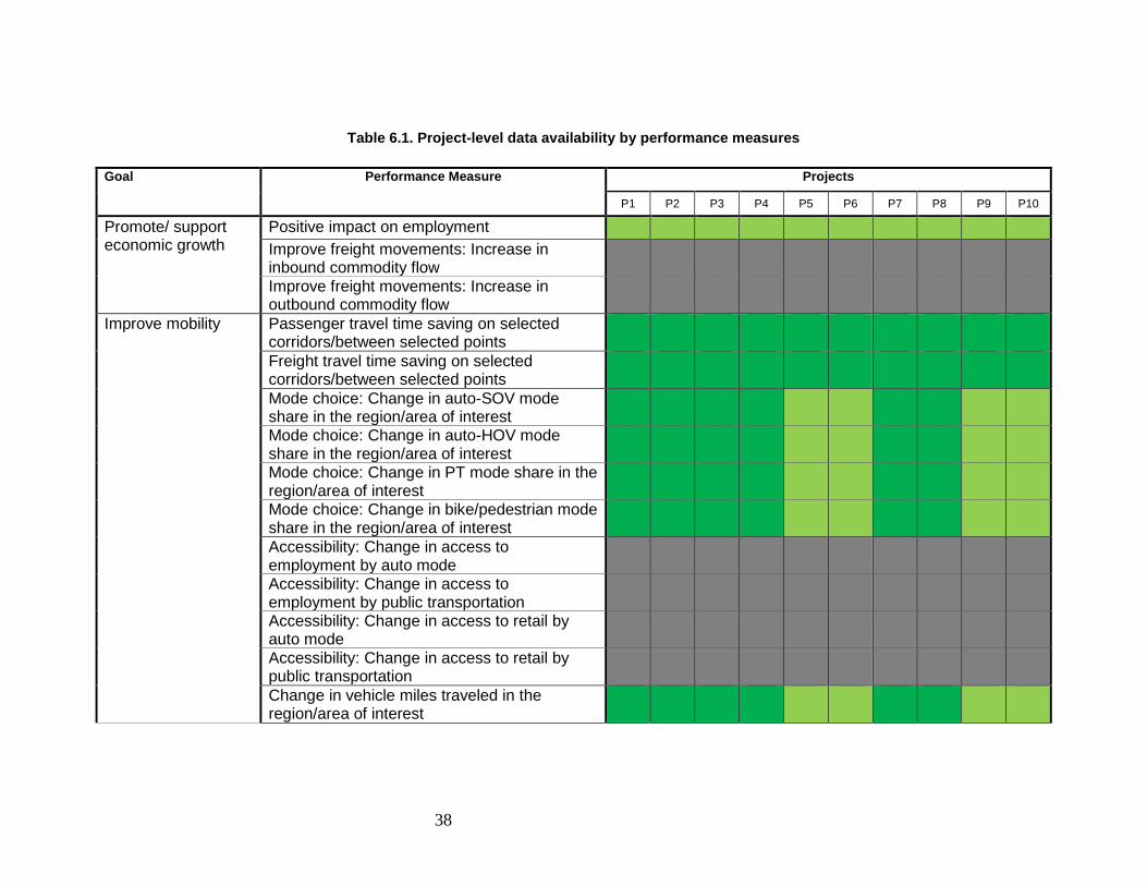
Table 6.1. Project-level data availability by performance measures

Goal Performance Measure Projects

P1 P2 P3 P4 P5 P6 P7 P8 P9 P10

Promote/ support economic growth

Positive impact on employment Improve freight movements: Increase in inbound commodity flow

Improve freight movements: Increase in outbound commodity flow

Improve mobility Passenger travel time saving on selected corridors/between selected points

Freight travel time saving on selected corridors/between selected points

Mode choice: Change in auto-SOV mode share in the region/area of interest

Mode choice: Change in auto-HOV mode share in the region/area of interest

Mode choice: Change in PT mode share in the region/area of interest

Mode choice: Change in bike/pedestrian mode share in the region/area of interest

Accessibility: Change in access to employment by auto mode

Accessibility: Change in access to employment by public transportation

Accessibility: Change in access to retail by auto mode

Accessibility: Change in access to retail by public transportation

Change in vehicle miles traveled in the region/area of interest

38

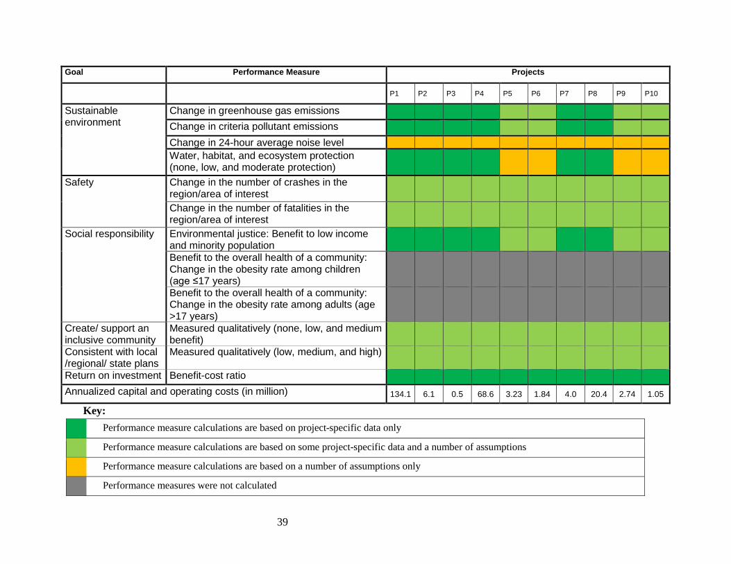
Goal Performance Measure Projects

P1 P2 P3 P4 P5 P6 P7 P8 P9 P10

Sustainable environment

Change in greenhouse gas emissions

Change in criteria pollutant emissions

Change in 24-hour average noise level

Water, habitat, and ecosystem protection (none, low, and moderate protection)

Safety Change in the number of crashes in the region/area of interest

Change in the number of fatalities in the region/area of interest

Social responsibility Environmental justice: Benefit to low income and minority population

Benefit to the overall health of a community: Change in the obesity rate among children (age ≤17 years)

Benefit to the overall health of a community: Change in the obesity rate among adults (age >17 years)

Create/ support an inclusive community

Measured qualitatively (none, low, and medium benefit)

Consistent with local /regional/ state plans

Measured qualitatively (low, medium, and high)

Return on investment Benefit-cost ratio Annualized capital and operating costs (in million) 134.1 6.1 0.5 68.6 3.23 1.84 4.0 20.4 2.74 1.05

Key: Performance measure calculations are based on project-specific data only

Performance measure calculations are based on some project-specific data and a number of assumptions

Performance measure calculations are based on a number of assumptions only

Performance measures were not calculated

39

6.3 Case Study 2: Hypothetical Case Study for FDA Technique FDA provides a holistic evaluation of the goods or services by surveying a group of decision-

makers or stakeholders and asking them to state their preferences for each of the goods or services to be allocated. Because no survey preference data was available for the projects employed in the hypothetical case study for DEA and CA techniques, we approached individual DOTs as to whether they had data that would support the FDA exercise. South Dakota’s DOT (SDDOT) provided a comprehensive study the state had conducted in 2011 to gain an understanding of residents’ and transportation decision-makers’ preferences regarding short-term and long-term priorities for the South Dakota DOT (SDDOT) (SDDOT 2011). These preferences are specific to South Dakota and reflect attitudes in a rural state with a large land area and a small, dispersed population.

SDDOT conducted a survey of residents and specific stakeholder groups in the spring of 2011; it documented the findings in the SDDOT 2011 Statewide Customer Satisfaction Assessment (SDDOT 2011). The resident survey was administered to 1,134 residents, while the stakeholder survey was administered to a wide variety of stakeholders, including 50 legislators. Both surveys consisted of a number of items about respondents’ preferences, including one item that acted as our input data for the FDA technique. This item focused on “several improvements that could be made to the transportation system in the State of South Dakota,” and respondents were asked to indicate “how important you think the improvement is by using a 5 point scale where ‘1’ is ‘very unimportant’ and ‘5’ is ‘very important’” (SDDOT 2011, Appendix C, p. 9). The item included 13 improvements, for which we included seven in our application of the FDA technique:

1. Expanding public transportation/bus service 2. Expanding transportation services for seniors and persons with disabilities 3. Relieving traffic congestion in cities such as Sioux Falls and Rapid City, 4. Adding turning and passing lanes to highways 5. Repairing and maintaining existing highways 6. Improving passenger bus service between cities 7. Improving the draining of water from the surface of highways when it rains.

These seven improvements were considered to be the projects in our hypothetical case study. Table 6.2 provides the mean ratings provided by residents and legislators that will act as inputs to the FDA technique.

40

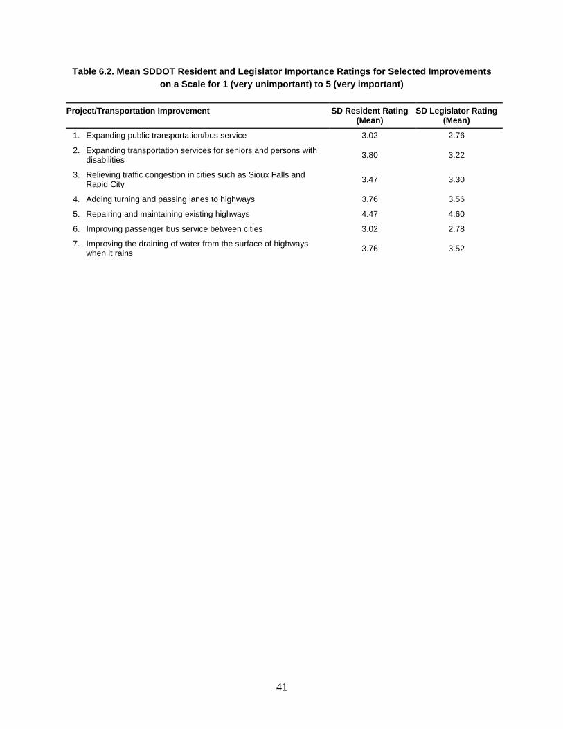
Table 6.2. Mean SDDOT Resident and Legislator Importance Ratings for Selected Improvements on a Scale for 1 (very unimportant) to 5 (very important)

Project/Transportation Improvement SD Resident Rating (Mean)

SD Legislator Rating (Mean)

1. Expanding public transportation/bus service 3.02 2.76

2. Expanding transportation services for seniors and persons with disabilities 3.80 3.22

3. Relieving traffic congestion in cities such as Sioux Falls and Rapid City 3.47 3.30

4. Adding turning and passing lanes to highways 3.76 3.56

5. Repairing and maintaining existing highways 4.47 4.60

6. Improving passenger bus service between cities 3.02 2.78

7. Improving the draining of water from the surface of highways when it rains 3.76 3.52

41

7. Application of DEA, CA, and FDA techniques

7.1 Introduction DEA, CA, and FDA techniques were applied in parallel to evaluate the case studies discussed

in Chapter 6. This chapter discusses the steps that were involved in applying each technique, evaluation results, and relative strengths and weaknesses of each technique. As we will see, each technique can help to inform transportation decision-making in a different way. These examples provide insight into how these techniques could be used if applied within state DOTs.

The DEA application, for instance, exemplifies that it is well-suited to transportation problems in which planners are evaluating the performance of many alternative existing or proposed activities; have access to quantitative measures of performance; have a relatively limited set of metrics they wish to use; and have some modeling expertise. DEA provides a quantitative method for evaluating performance and making investment decisions (for example, if the projects or activities already exist, DEA can suggest where management action is required to improve performance; if the projects are proposed, DEA can show which offer the greatest return on investment).

On the other hand, conjoint analysis can be especially useful when assessing competing projects that offer multiple monetary and non-monetary benefits. This is an important advantage since transportation projects that are typically considered for STIP can vary widely in the types of monetary and non-monetary benefits they offer. Thus, applying dollar benefits alone to prioritize transportation projects for funding consideration may not result in a mix of projects that address an agency’s goals and objectives and that offer the most benefits to the community.

Finally, FDA provides a means of allocating resources without the use of numerical computational tools or any special expertise on the part of the analyst. Therefore, if a state DOT does not have resources to invest in statistical tools or expertise, using FDA allows for a method for resource allocation that does not require this investment. The technique also incorporates the opinions of multiple stakeholders into the allocation decision. Thus, the technique may be especially helpful when the resource allocation will affect many stakeholders and transportation decision-makers want to ensure that the final allocation is “fair” for all stakeholder groups involved.

7.2 Data Envelopment Analysis (DEA) In this section, we present an application of Data Envelopment Analysis, using the

transportation project data discussed in the previous chapter.

43

In this analysis, we imagine transportation planners comparing alternative transportation infrastructure investment projects. Decision-makers are faced with the complex task of evaluating multiple alternatives along many dimensions; each alternative project requires different levels of annual operating costs, and will produce a variety of different outputs.

DEA can be an effective tool for this task because of its ability to compare alternatives that may perform very differently along different metrics (for example, one project might reduce traffic fatalities while another might create jobs). But the formulation of the DEA problem places certain restrictions on the quantity and type of data needed, which may make using DEA inappropriate in some cases.7

In what follows, we will explore the applicability of DEA to the task of evaluating the transportation investment projects provided in the sample dataset. In the process, we will conduct an analysis using DEA, discuss some of its practical limitations, and identify potential mitigation strategies.

Modeling Project Attributes

DEA classifies each project attribute as either an input or an output. In general, attributes should be classified as either inputs or outputs in a manner that is consistent with their real-world interpretation. For example, a natural choice for a project attribute that could be modeled as an input would be project annual operating cost. Natural choices for outputs are travel time savings or freight time savings, among several others. Generally speaking, attributes that correspond to costs (financial or otherwise) should be modeled as inputs, while attributes that correspond to benefits should be modeled as outputs.

A simple DEA analysis – one input and one output

DEA compares the ratio of outputs to inputs for each project, but the specific weights (relative value) assigned to each input and output are unique to each project and are set to allow the project to appear as efficient as possible relative to is peers (this avoids making any assumptions about the relative value of inputs or outputs). Because we are working with only one input and one output in this example, all weights are set to 1.0.

Figure 5.1 below plots each of the candidate projects based on their travel-time savings as a function of their annual operating costs. The variable-returns-to-scale model is usually more realistic for most applications, and it is this model that was used to generate the plot below.8

7 For example, project attributes should, in general, be quantifiable and non-negative. The candidate projects should outnumber the attributes used to describe the projects by a significant margin. These issues, and strategies for addressing the attributes, are discussed in greater detail in subsequent sections. 8 For an overview of alternative approaches to returns-to-scale, see Banker, Rajiv D., William W. Cooper, Lawrence M. Seiford, Robert M. Thrall, and Joe Zhu, “Returns to Scale in Different DEA Models.” European Journal of Operational Research 154, no. 2 (2004): 345-62.

44

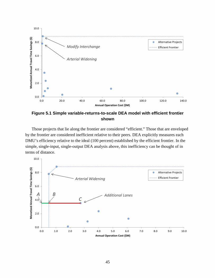
Figure 5.1 Simple variable-returns-to-scale DEA model with efficient frontier shown

Those projects that lie along the frontier are considered “efficient.” Those that are enveloped by the frontier are considered inefficient relative to their peers. DEA explicitly measures each DMU’s efficiency relative to the ideal (100 percent) established by the efficient frontier. In the simple, single-input, single-output DEA analysis above, this inefficiency can be thought of in terms of distance.

Arterial Widening

Modify Interchange

0.0

2.0

4.0

6.0

8.0

10.0

0.0 20.0 40.0 60.0 80.0 100.0 120.0 140.0

Mon

etiz

ed A

nnua

l Tra

vel T

ime

Savi

ngs

($)

Annual Operation Cost ($M)

Alternative Projects

Efficient Frontier

0.0

2.0

4.0

6.0

8.0

10.0

0.0 1.0 2.0 3.0 4.0 5.0 6.0 7.0 8.0 9.0 10.0

Mon

etiz

ed A

nnua

l Tra

vel T

ime

Savi

ngs

($)

Annual Operation Cost ($M)

Alternative Projects

Efficient Frontier

A BC

Arterial Widening

Additional Lanes

45

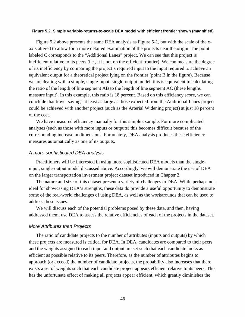
Figure 5.2. Simple variable-returns-to-scale DEA model with efficient frontier shown (magnified)

Figure 5.2 above presents the same DEA analysis as Figure 5-1, but with the scale of the x-axis altered to allow for a more detailed examination of the projects near the origin. The point labeled C corresponds to the “Additional Lanes” project. We can see that this project is inefficient relative to its peers (i.e., it is not on the efficient frontier). We can measure the degree of its inefficiency by comparing the project’s required input to the input required to achieve an equivalent output for a theoretical project lying on the frontier (point B in the figure). Because we are dealing with a simple, single-input, single-output model, this is equivalent to calculating the ratio of the length of line segment AB to the length of line segment AC (these lengths measure input). In this example, this ratio is 18 percent. Based on this efficiency score, we can conclude that travel savings at least as large as those expected from the Additional Lanes project could be achieved with another project (such as the Arterial Widening project) at just 18 percent of the cost.

We have measured efficiency manually for this simple example. For more complicated analyses (such as those with more inputs or outputs) this becomes difficult because of the corresponding increase in dimensions. Fortunately, DEA analysis produces these efficiency measures automatically as one of its outputs.

A more sophisticated DEA analysis

Practitioners will be interested in using more sophisticated DEA models than the single-input, single-output model discussed above. Accordingly, we will demonstrate the use of DEA on the larger transportation investment project dataset introduced in Chapter 2.

The nature and size of this dataset present a variety of challenges to DEA. While perhaps not ideal for showcasing DEA’s strengths, these data do provide a useful opportunity to demonstrate some of the real-world challenges of using DEA, as well as the workarounds that can be used to address these issues.

We will discuss each of the potential problems posed by these data, and then, having addressed them, use DEA to assess the relative efficiencies of each of the projects in the dataset.

More Attributes than Projects

The ratio of candidate projects to the number of attributes (inputs and outputs) by which these projects are measured is critical for DEA. In DEA, candidates are compared to their peers and the weights assigned to each input and output are set such that each candidate looks as efficient as possible relative to its peers. Therefore, as the number of attributes begins to approach (or exceed) the number of candidate projects, the probability also increases that there exists a set of weights such that each candidate project appears efficient relative to its peers. This has the unfortunate effect of making all projects appear efficient, which greatly diminishes the

46

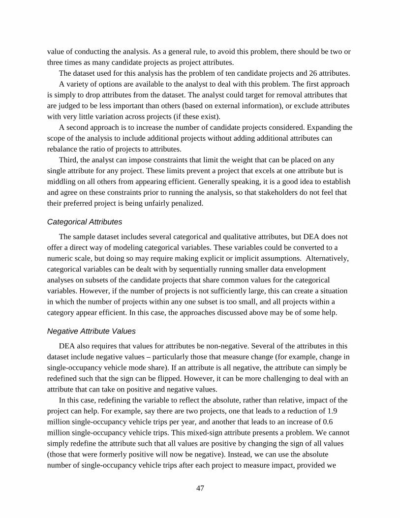
value of conducting the analysis. As a general rule, to avoid this problem, there should be two or three times as many candidate projects as project attributes.

The dataset used for this analysis has the problem of ten candidate projects and 26 attributes. A variety of options are available to the analyst to deal with this problem. The first approach

is simply to drop attributes from the dataset. The analyst could target for removal attributes that are judged to be less important than others (based on external information), or exclude attributes with very little variation across projects (if these exist).

A second approach is to increase the number of candidate projects considered. Expanding the scope of the analysis to include additional projects without adding additional attributes can rebalance the ratio of projects to attributes.

Third, the analyst can impose constraints that limit the weight that can be placed on any single attribute for any project. These limits prevent a project that excels at one attribute but is middling on all others from appearing efficient. Generally speaking, it is a good idea to establish and agree on these constraints prior to running the analysis, so that stakeholders do not feel that their preferred project is being unfairly penalized.

Categorical Attributes

The sample dataset includes several categorical and qualitative attributes, but DEA does not offer a direct way of modeling categorical variables. These variables could be converted to a numeric scale, but doing so may require making explicit or implicit assumptions. Alternatively, categorical variables can be dealt with by sequentially running smaller data envelopment analyses on subsets of the candidate projects that share common values for the categorical variables. However, if the number of projects is not sufficiently large, this can create a situation in which the number of projects within any one subset is too small, and all projects within a category appear efficient. In this case, the approaches discussed above may be of some help.

Negative Attribute Values

DEA also requires that values for attributes be non-negative. Several of the attributes in this dataset include negative values – particularly those that measure change (for example, change in single-occupancy vehicle mode share). If an attribute is all negative, the attribute can simply be redefined such that the sign can be flipped. However, it can be more challenging to deal with an attribute that can take on positive and negative values.

In this case, redefining the variable to reflect the absolute, rather than relative, impact of the project can help. For example, say there are two projects, one that leads to a reduction of 1.9 million single-occupancy vehicle trips per year, and another that leads to an increase of 0.6 million single-occupancy vehicle trips. This mixed-sign attribute presents a problem. We cannot simply redefine the attribute such that all values are positive by changing the sign of all values (those that were formerly positive will now be negative). Instead, we can use the absolute number of single-occupancy vehicle trips after each project to measure impact, provided we

47

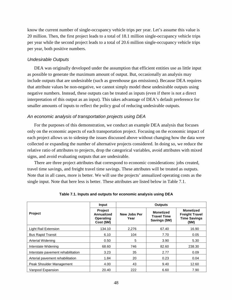
know the current number of single-occupancy vehicle trips per year. Let’s assume this value is 20 million. Then, the first project leads to a total of 18.1 million single-occupancy vehicle trips per year while the second project leads to a total of 20.6 million single-occupancy vehicle trips per year, both positive numbers.

Undesirable Outputs

DEA was originally developed under the assumption that efficient entities use as little input as possible to generate the maximum amount of output. But, occasionally an analysis may include outputs that are undesirable (such as greenhouse gas emissions). Because DEA requires that attribute values be non-negative, we cannot simply model these undesirable outputs using negative numbers. Instead, these outputs can be treated as inputs (even if there is not a direct interpretation of this output as an input). This takes advantage of DEA’s default preference for smaller amounts of inputs to reflect the policy goal of reducing undesirable outputs.

An economic analysis of transportation projects using DEA

For the purposes of this demonstration, we conduct an example DEA analysis that focuses only on the economic aspects of each transportation project. Focusing on the economic impact of each project allows us to sidestep the issues discussed above without changing how the data were collected or expanding the number of alternative projects considered. In doing so, we reduce the relative ratio of attributes to projects, drop the categorical variables, avoid attributes with mixed signs, and avoid evaluating outputs that are undesirable.

There are three project attributes that correspond to economic considerations: jobs created, travel time savings, and freight travel time savings. These attributes will be treated as outputs. Note that in all cases, more is better. We will use the projects’ annualized operating costs as the single input. Note that here less is better. These attributes are listed below in Table 7.1.

Table 7.1. Inputs and outputs for economic analysis using DEA

Project

Input Outputs Project

Annualized Operating Cost ($M)

New Jobs Per Year

Monetized Travel Time

Savings ($M)

Monetized Freight Travel Time Savings

($M)

Light Rail Extension 134.10 2,276 67.40 16.90

Bus Rapid Transit 6.10 104 7.70 0.05

Arterial Widening 0.50 5 3.90 5.30

Interstate Widening 68.60 746 82.60 238.30

Interstate pavement rehabilitation 3.23 35 2.77 0.09

Arterial pavement rehabilitation 1.84 20 0.23 0.04

Peak Shoulder Management 4.00 43 9.40 12.60

Vanpool Expansion 20.40 222 6.60 7.90

48

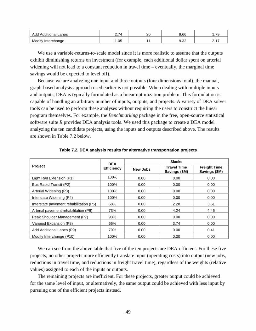
Add Additional Lanes 2.74 30 9.66 1.79

Modify Interchange 1.05 11 9.32 2.17 We use a variable-returns-to-scale model since it is more realistic to assume that the outputs

exhibit diminishing returns on investment (for example, each additional dollar spent on arterial widening will not lead to a constant reduction in travel time – eventually, the marginal time savings would be expected to level off).

Because we are analyzing one input and three outputs (four dimensions total), the manual, graph-based analysis approach used earlier is not possible. When dealing with multiple inputs and outputs, DEA is typically formulated as a linear optimization problem. This formulation is capable of handling an arbitrary number of inputs, outputs, and projects. A variety of DEA solver tools can be used to perform these analyses without requiring the users to construct the linear program themselves. For example, the Benchmarking package in the free, open-source statistical software suite R provides DEA analysis tools. We used this package to create a DEA model analyzing the ten candidate projects, using the inputs and outputs described above. The results are shown in Table 7.2 below.

Table 7.2. DEA analysis results for alternative transportation projects

Project DEA Efficiency

Slacks

New Jobs Travel Time Savings ($M)

Freight Time Savings ($M)

Light Rail Extension (P1) 100% 0.00 0.00 0.00

Bus Rapid Transit (P2) 100% 0.00 0.00 0.00

Arterial Widening (P3) 100% 0.00 0.00 0.00

Interstate Widening (P4) 100% 0.00 0.00 0.00

Interstate pavement rehabilitation (P5) 68% 0.00 2.28 3.61

Arterial pavement rehabilitation (P6) 73% 0.00 4.24 4.46

Peak Shoulder Management (P7) 93% 0.00 0.00 0.00

Vanpool Expansion (P8) 66% 0.00 3.74 0.00

Add Additional Lanes (P9) 79% 0.00 0.00 0.41

Modify Interchange (P10) 100% 0.00 0.00 0.00 We can see from the above table that five of the ten projects are DEA-efficient. For these five

projects, no other projects more efficiently translate input (operating costs) into output (new jobs, reductions in travel time, and reductions in freight travel time), regardless of the weights (relative values) assigned to each of the inputs or outputs.

The remaining projects are inefficient. For these projects, greater output could be achieved for the same level of input, or alternatively, the same output could be achieved with less input by pursuing one of the efficient projects instead.

49

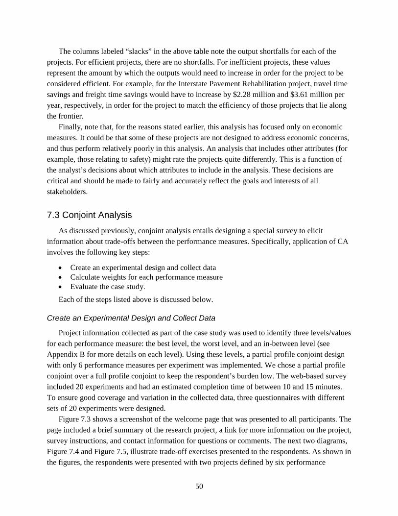
The columns labeled “slacks” in the above table note the output shortfalls for each of the projects. For efficient projects, there are no shortfalls. For inefficient projects, these values represent the amount by which the outputs would need to increase in order for the project to be considered efficient. For example, for the Interstate Pavement Rehabilitation project, travel time savings and freight time savings would have to increase by $2.28 million and $3.61 million per year, respectively, in order for the project to match the efficiency of those projects that lie along the frontier.

Finally, note that, for the reasons stated earlier, this analysis has focused only on economic measures. It could be that some of these projects are not designed to address economic concerns, and thus perform relatively poorly in this analysis. An analysis that includes other attributes (for example, those relating to safety) might rate the projects quite differently. This is a function of the analyst’s decisions about which attributes to include in the analysis. These decisions are critical and should be made to fairly and accurately reflect the goals and interests of all stakeholders.

7.3 Conjoint Analysis As discussed previously, conjoint analysis entails designing a special survey to elicit

information about trade-offs between the performance measures. Specifically, application of CA involves the following key steps:

• Create an experimental design and collect data • Calculate weights for each performance measure • Evaluate the case study. Each of the steps listed above is discussed below.

Create an Experimental Design and Collect Data

Project information collected as part of the case study was used to identify three levels/values for each performance measure: the best level, the worst level, and an in-between level (see Appendix B for more details on each level). Using these levels, a partial profile conjoint design with only 6 performance measures per experiment was implemented. We chose a partial profile conjoint over a full profile conjoint to keep the respondent’s burden low. The web-based survey included 20 experiments and had an estimated completion time of between 10 and 15 minutes. To ensure good coverage and variation in the collected data, three questionnaires with different sets of 20 experiments were designed.

Figure 7.3 shows a screenshot of the welcome page that was presented to all participants. The page included a brief summary of the research project, a link for more information on the project, survey instructions, and contact information for questions or comments. The next two diagrams, Figure 7.4 and Figure 7.5, illustrate trade-off exercises presented to the respondents. As shown in the figures, the respondents were presented with two projects defined by six performance

50

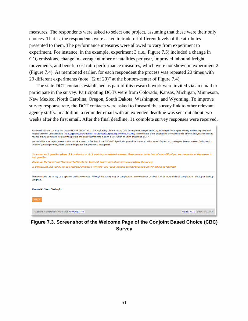
measures. The respondents were asked to select one project, assuming that these were their only choices. That is, the respondents were asked to trade-off different levels of the attributes presented to them. The performance measures were allowed to vary from experiment to experiment. For instance, in the example, experiment 3 (i.e., Figure 7.5) included a change in CO2 emissions, change in average number of fatalities per year, improved inbound freight movements, and benefit cost ratio performance measures, which were not shown in experiment 2 (Figure 7.4). As mentioned earlier, for each respondent the process was repeated 20 times with 20 different experiments (note “(2 of 20)” at the bottom-center of Figure 7.4).

The state DOT contacts established as part of this research work were invited via an email to participate in the survey. Participating DOTs were from Colorado, Kansas, Michigan, Minnesota, New Mexico, North Carolina, Oregon, South Dakota, Washington, and Wyoming. To improve survey response rate, the DOT contacts were asked to forward the survey link to other relevant agency staffs. In addition, a reminder email with an extended deadline was sent out about two weeks after the first email. After the final deadline, 11 complete survey responses were received.

Figure 7.3. Screenshot of the Welcome Page of the Conjoint Based Choice (CBC) Survey

51

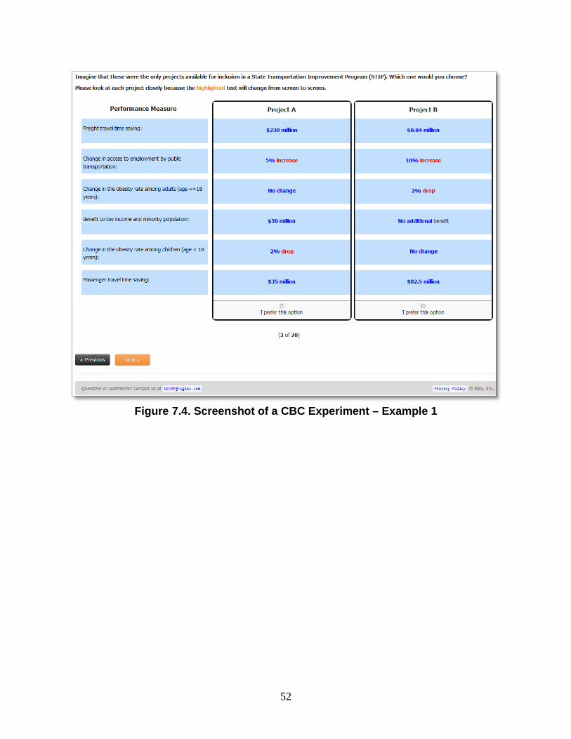
Figure 7.4. Screenshot of a CBC Experiment – Example 1

52

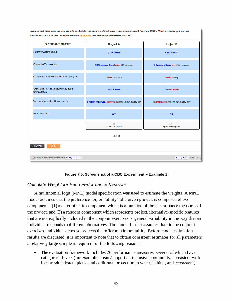
Figure 7.5. Screenshot of a CBC Experiment – Example 2

Calculate Weight for Each Performance Measure

A multinomial logit (MNL) model specification was used to estimate the weights. A MNL model assumes that the preference for, or “utility” of a given project, is composed of two components: (1) a deterministic component which is a function of the performance measures of the project, and (2) a random component which represents project/alternative-specific features that are not explicitly included in the conjoint exercises or general variability in the way that an individual responds to different alternatives. The model further assumes that, in the conjoint exercises, individuals choose projects that offer maximum utility. Before model estimation results are discussed, it is important to note that to obtain consistent estimates for all parameters a relatively large sample is required for the following reasons:

• The evaluation framework includes 26 performance measures, several of which have categorical levels (for example, create/support an inclusive community, consistent with local/regional/state plans, and additional protection to water, habitat, and ecosystem).

53

• In an effort to keep the number of performance measures presented per experiment at a reasonable level, only six performance measures were shown at a time.

• Correlations across observations exist due to the panel nature of the data (each respondent participated in 20 experiments).

However, the sample size for the current analysis is 11, which is too small to provide consistent estimates for all parameters. On the other hand, the current research is a proof of concept. Therefore, it is not crucial to the project objectives for the estimated parameters to be consistent.

Model estimation results are presented in Table 7.3. Because none of the estimated parameters were statistically significantly different from zero, the model results are summarized in terms of the signs of the coefficients and whether or not the coefficients have intuitive sign. As can be observed from the table, about half of the parameters have signs that are intuitive. It is likely the parameters that have counterintuitive signs, as well as some of the parameters that have intuitive signs, represent attributes that were relatively unimportant to those who completed the survey. From a statistical standpoint, issues such as correlation and confounding also could result in parameters with counterintuitive signs. In general, these effects can be more easily distinguished with larger sample sizes or by testing smaller numbers of attributes.

Evaluate the Case Study

To evaluate the case study, the utility of each project was calculated as follows:

𝑈𝑈𝑈𝑈𝑈𝑈𝑈𝑈𝑈𝑈𝑈𝑈𝑈𝑈 𝑜𝑜𝑜𝑜 𝑃𝑃𝑃𝑃𝑜𝑜𝑃𝑃𝑃𝑃𝑃𝑃𝑈𝑈 𝑈𝑈 = �𝛽𝛽𝑗𝑗

26

𝑗𝑗=1

𝑋𝑋𝑖𝑖𝑗𝑗

Where, i = 1, 2, …,10; βj is the coefficient for performance measure j, and Xij is the value of performance measure j for project i. It should be noted that for practical implementation purposes the following steps were applied when calculating project utilities:

• Categorical performance measures where the estimated parameters were not intuitive across the categories (create/support an inclusive community consistent with local/regional/state plans), βj values for the lower categories were adopted for the upper categories.

• βj values were set to zero for all other parameters with counterintuitive signs.

Next, the relative preferences among the projects were calculated as follows:

𝑃𝑃𝑃𝑃𝑃𝑃𝑃𝑃𝑃𝑃𝑃𝑃𝑈𝑈𝑃𝑃𝑃𝑃𝑃𝑃 𝑃𝑃𝑃𝑃𝑈𝑈𝑃𝑃𝑈𝑈𝑈𝑈𝑟𝑟𝑃𝑃 𝑝𝑝𝑃𝑃𝑃𝑃𝑜𝑜𝑃𝑃𝑃𝑃𝑃𝑃𝑃𝑃𝑃𝑃𝑃𝑃 𝑜𝑜𝑜𝑜𝑃𝑃 𝑝𝑝𝑃𝑃𝑜𝑜𝑃𝑃𝑃𝑃𝑃𝑃𝑈𝑈 𝑈𝑈,𝑃𝑃𝑖𝑖 =𝑃𝑃𝑈𝑈𝑈𝑈𝑖𝑖𝑈𝑈𝑖𝑖𝑈𝑈𝑈𝑈 𝑜𝑜𝑜𝑜 𝑃𝑃𝑃𝑃𝑜𝑜𝑗𝑗𝑃𝑃𝑃𝑃𝑈𝑈𝑖𝑖

∑ 𝑃𝑃𝑈𝑈𝑈𝑈𝑖𝑖𝑈𝑈𝑖𝑖𝑈𝑈𝑈𝑈 𝑜𝑜𝑜𝑜 𝑃𝑃𝑃𝑃𝑜𝑜𝑗𝑗𝑃𝑃𝑃𝑃𝑈𝑈𝑖𝑖10𝑖𝑖=1

× 100

Calculated statistics are presented in Figure 7.6. As shown in the figure, in addition to ranking the projects, the CA technique may also be used to determine relative preferences among the projects. Further, this technique may be applied to identify the performance measures that contribute most to overall project rating (see Table 7.4). For example, CA analysis results

54

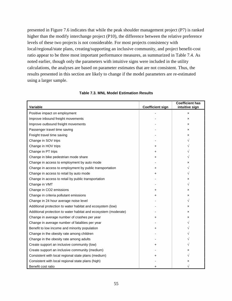
presented in Figure 7.6 indicates that while the peak shoulder management project (P7) is ranked higher than the modify interchange project (P10), the difference between the relative preference levels of these two projects is not considerable. For most projects consistency with local/regional/state plans, creating/supporting an inclusive community, and project benefit-cost ratio appear to be three most important performance measures, as summarized in Table 7.4. As noted earlier, though only the parameters with intuitive signs were included in the utility calculations, the analyses are based on parameter estimates that are not consistent. Thus, the results presented in this section are likely to change if the model parameters are re-estimated using a larger sample.

Table 7.3. MNL Model Estimation Results

Variable Coefficient sign Coefficient has intuitive sign

Positive impact on employment - × Improve inbound freight movements - × Improve outbound freight movements - × Passenger travel time saving - × Freight travel time saving - × Change in SOV trips - √ Change in HOV trips + √ Change in PT trips + √ Change in bike pedestrian mode share + √ Change in access to employment by auto mode - × Change in access to employment by public transportation + √ Change in access to retail by auto mode + √ Change in access to retail by public transportation - × Change in VMT - √ Change in CO2 emissions + × Change in criteria pollutant emissions + × Change in 24 hour average noise level - √ Additional protection to water habitat and ecosystem (low) - × Additional protection to water habitat and ecosystem (moderate) - × Change in average number of crashes per year + × Change in average number of fatalities per year - √ Benefit to low income and minority population + √ Change in the obesity rate among children - √ Change in the obesity rate among adults - √ Create support an inclusive community (low) + √ Create support an inclusive community (medium) - × Consistent with local regional state plans (medium) + √ Consistent with local regional state plans (high) - × Benefit cost ratio + √

55

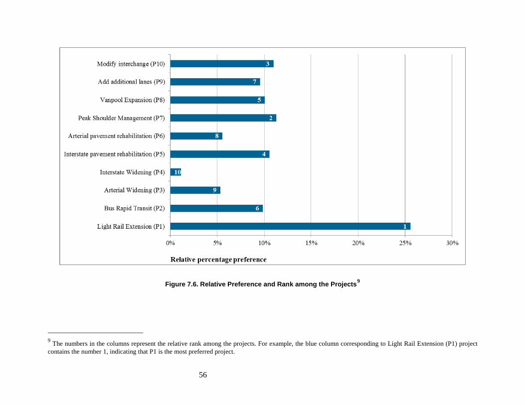
Figure 7.6. Relative Preference and Rank among the Projects9

9 The numbers in the columns represent the relative rank among the projects. For example, the blue column corresponding to Light Rail Extension (P1) project contains the number 1, indicating that P1 is the most preferred project.

56

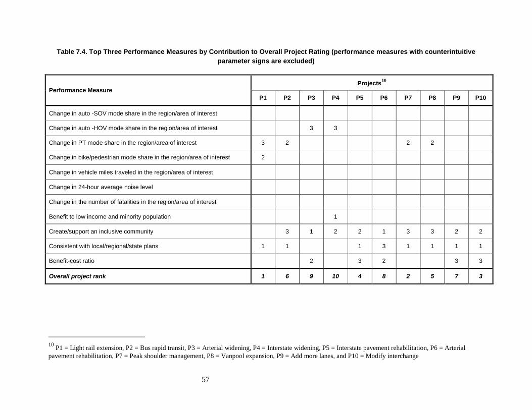
Table 7.4. Top Three Performance Measures by Contribution to Overall Project Rating (performance measures with counterintuitive parameter signs are excluded)

Performance Measure Projects10

P1 P2 P3 P4 P5 P6 P7 P8 P9 P10

Change in auto -SOV mode share in the region/area of interest

Change in auto -HOV mode share in the region/area of interest 3 3

Change in PT mode share in the region/area of interest 3 2 2 2

Change in bike/pedestrian mode share in the region/area of interest 2

Change in vehicle miles traveled in the region/area of interest

Change in 24-hour average noise level

Change in the number of fatalities in the region/area of interest

Benefit to low income and minority population 1

Create/support an inclusive community 3 1 2 2 1 3 3 2 2

Consistent with local/regional/state plans 1 1 1 3 1 1 1 1

Benefit-cost ratio 2 3 2 3 3

Overall project rank 1 6 9 10 4 8 2 5 7 3

10 P1 = Light rail extension, P2 = Bus rapid transit, P3 = Arterial widening, P4 = Interstate widening, P5 = Interstate pavement rehabilitation, P6 = Arterial pavement rehabilitation, P7 = Peak shoulder management, P8 = Vanpool expansion, P9 = Add more lanes, and P10 = Modify interchange

57

7.4 Fair Division Analysis For this application of FDA, we employed a method similar to that of Kiryluk (2013). The

method includes a number of steps, which provide an extension of the Divide the Dollar game, as described in Brams and Taylor (1994) and Brams (2008). The process is reproduced in a flow chart shown in Figure 7-7, and involves the following steps:

• First, mean preferences for each stakeholder group are obtained at the project level. • Next, to enable comparisons between stakeholder preferences, these mean ratings are

standardized using a Z-score method: 𝑥𝑥� = 𝑥𝑥−𝜇𝜇𝜎𝜎

, where x is the mean rating for one project, μ is the average of the mean ratings across all projects within a stakeholder group and σ is the standard deviation for the mean ratings within a stakeholder group.

• Third, the number of beneficiaries is obtained for each project.11 This is combined with an objective measure of the unit of payment per beneficiary to identify upper and lower bounds for financing each project. The assignment of upper and lower bounds is described in more detail below.

• Next, following Brams and Taylor (1994), the sequence of payments is determined by subtracting the standardized ratings of the stakeholder group designated as the beneficiary from the (average12) standardized ratings of the other stakeholder group(s). By ordering payments in these terms, the algorithm results in the projects that are most overestimated by beneficiaries being at risk of not being funded (above any lower bound that is set).

• Next, the payments for projects are determined as a fraction of the upper bound for that project that is proportional to beneficiaries’ relative preference for that project. Thus, funding is allocated to projects according to beneficiaries’ preferences. No project may receive more financing than its upper bound, but must receive an amount at least equal to that of its lower bound. If total funding is depleted before all projects have received their payment in the rotation, financing is reallocated such that the lower bounds for each of the remaining projects are met. On the other hand, if financing is not depleted after satisfying the beneficiaries’ requests, the remaining funds are divided proportionally among all projects that have not yet reached their upper bounds.

11 For the purposes of this application, a beneficiary is someone who directly benefits from the project (likely through making use of the good or service provided). For instance, senior citizens would be considered beneficiaries of projects that improve services for the elderly. Individuals not considered to be beneficiaries are those to do not receive direct benefits from the project. For instance, a policy-maker or transportation planner would be considered a non-beneficiary for this application. 12 If more than one non-beneficiary stakeholder group is included in the analysis.

59

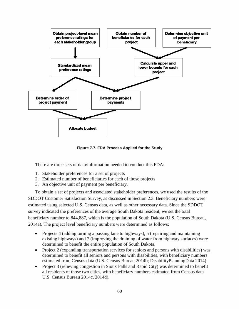
Figure 7.7. FDA Process Applied for the Study

There are three sets of data/information needed to conduct this FDA:

1. Stakeholder preferences for a set of projects 2. Estimated number of beneficiaries for each of those projects 3. An objective unit of payment per beneficiary.

To obtain a set of projects and associated stakeholder preferences, we used the results of the SDDOT Customer Satisfaction Survey, as discussed in Section 2.3. Beneficiary numbers were estimated using selected U.S. Census data, as well as other necessary data. Since the SDDOT survey indicated the preferences of the average South Dakota resident, we set the total beneficiary number to 844,887, which is the population of South Dakota (U.S. Census Bureau, 2014a). The project level beneficiary numbers were determined as follows:

• Projects 4 (adding turning a passing lane to highways), 5 (repairing and maintaining existing highways) and 7 (improving the draining of water from highway surfaces) were determined to benefit the entire population of South Dakota.

• Project 2 (expanding transportation services for seniors and persons with disabilities) was determined to benefit all seniors and persons with disabilities, with beneficiary numbers estimated from Census data (U.S. Census Bureau 2014b; DisabilityPlanningData 2014).

• Project 3 (relieving congestion in Sioux Falls and Rapid City) was determined to benefit all residents of those two cities, with beneficiary numbers estimated from Census data U.S. Census Bureau 2014c, 2014d).

60

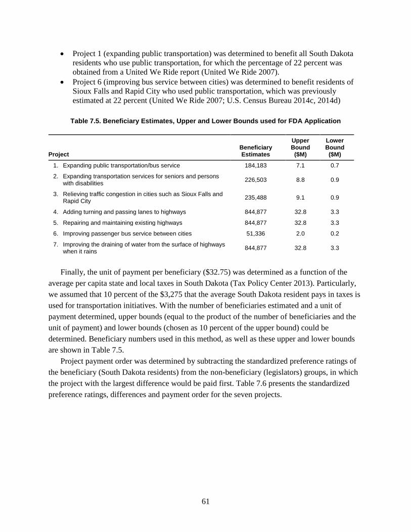
• Project 1 (expanding public transportation) was determined to benefit all South Dakota residents who use public transportation, for which the percentage of 22 percent was obtained from a United We Ride report (United We Ride 2007).

• Project 6 (improving bus service between cities) was determined to benefit residents of Sioux Falls and Rapid City who used public transportation, which was previously estimated at 22 percent (United We Ride 2007; U.S. Census Bureau 2014c, 2014d)

Table 7.5. Beneficiary Estimates, Upper and Lower Bounds used for FDA Application

Project Beneficiary Estimates

Upper Bound

($M)

Lower Bound

($M)

1. Expanding public transportation/bus service 184,183 7.1 0.7

2. Expanding transportation services for seniors and persons with disabilities 226,503 8.8 0.9

3. Relieving traffic congestion in cities such as Sioux Falls and Rapid City 235,488 9.1 0.9

4. Adding turning and passing lanes to highways 844,877 32.8 3.3

5. Repairing and maintaining existing highways 844,877 32.8 3.3

6. Improving passenger bus service between cities 51,336 2.0 0.2

7. Improving the draining of water from the surface of highways when it rains 844,877 32.8 3.3

Finally, the unit of payment per beneficiary ($32.75) was determined as a function of the

average per capita state and local taxes in South Dakota (Tax Policy Center 2013). Particularly, we assumed that 10 percent of the $3,275 that the average South Dakota resident pays in taxes is used for transportation initiatives. With the number of beneficiaries estimated and a unit of payment determined, upper bounds (equal to the product of the number of beneficiaries and the unit of payment) and lower bounds (chosen as 10 percent of the upper bound) could be determined. Beneficiary numbers used in this method, as well as these upper and lower bounds are shown in Table 7.5.

Project payment order was determined by subtracting the standardized preference ratings of the beneficiary (South Dakota residents) from the non-beneficiary (legislators) groups, in which the project with the largest difference would be paid first. Table 7.6 presents the standardized preference ratings, differences and payment order for the seven projects.

61

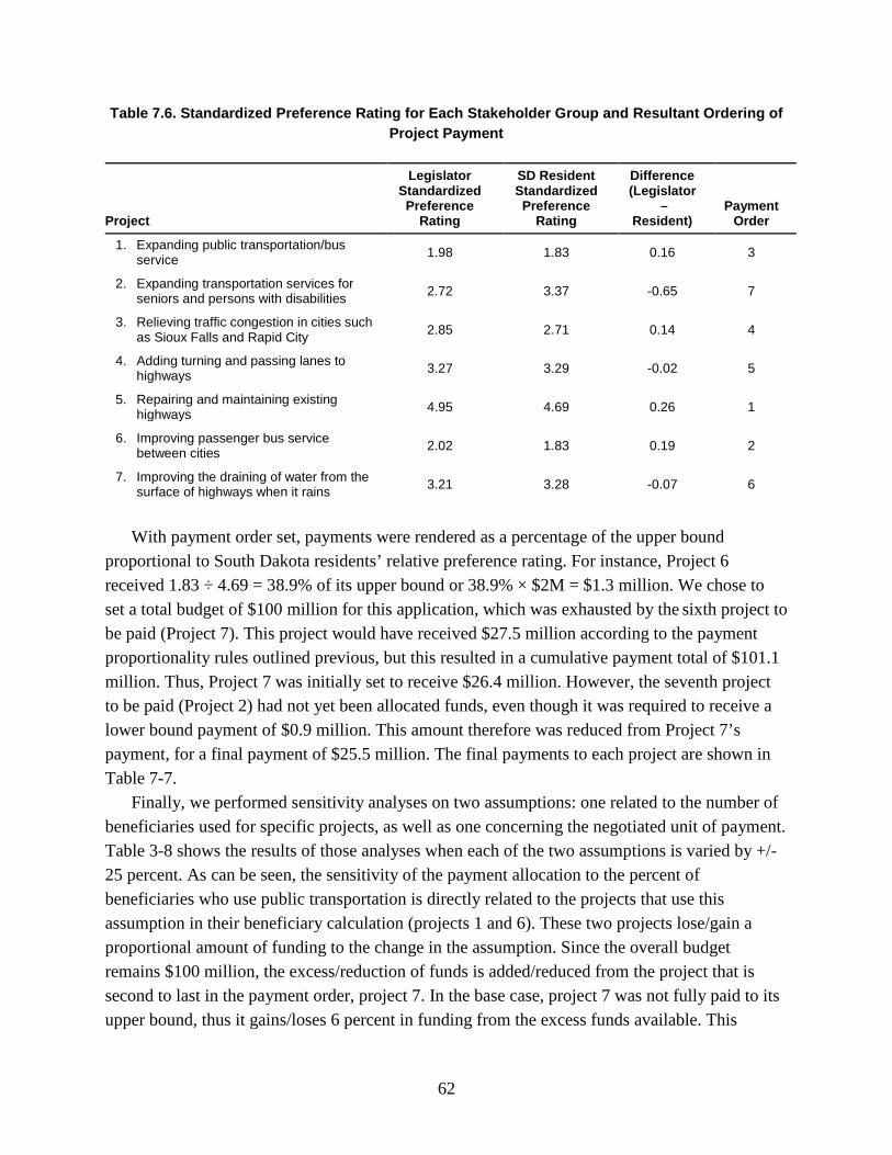
Table 7.6. Standardized Preference Rating for Each Stakeholder Group and Resultant Ordering of Project Payment

Project

Legislator Standardized Preference

Rating

SD Resident Standardized Preference

Rating

Difference (Legislator

– Resident)

Payment Order

1. Expanding public transportation/bus service 1.98 1.83 0.16 3

2. Expanding transportation services for seniors and persons with disabilities 2.72 3.37 -0.65 7

3. Relieving traffic congestion in cities such as Sioux Falls and Rapid City 2.85 2.71 0.14 4

4. Adding turning and passing lanes to highways 3.27 3.29 -0.02 5

5. Repairing and maintaining existing highways 4.95 4.69 0.26 1

6. Improving passenger bus service between cities 2.02 1.83 0.19 2

7. Improving the draining of water from the surface of highways when it rains 3.21 3.28 -0.07 6

With payment order set, payments were rendered as a percentage of the upper bound

proportional to South Dakota residents’ relative preference rating. For instance, Project 6 received 1.83 ÷ 4.69 = 38.9% of its upper bound or 38.9% × $2M = $1.3 million. We chose to set a total budget of $100 million for this application, which was exhausted by the sixth project to be paid (Project 7). This project would have received $27.5 million according to the payment proportionality rules outlined previous, but this resulted in a cumulative payment total of $101.1 million. Thus, Project 7 was initially set to receive $26.4 million. However, the seventh project to be paid (Project 2) had not yet been allocated funds, even though it was required to receive a lower bound payment of $0.9 million. This amount therefore was reduced from Project 7’s payment, for a final payment of $25.5 million. The final payments to each project are shown in Table 7-7.

Finally, we performed sensitivity analyses on two assumptions: one related to the number of beneficiaries used for specific projects, as well as one concerning the negotiated unit of payment. Table 3-8 shows the results of those analyses when each of the two assumptions is varied by +/-25 percent. As can be seen, the sensitivity of the payment allocation to the percent of beneficiaries who use public transportation is directly related to the projects that use this assumption in their beneficiary calculation (projects 1 and 6). These two projects lose/gain a proportional amount of funding to the change in the assumption. Since the overall budget remains $100 million, the excess/reduction of funds is added/reduced from the project that is second to last in the payment order, project 7. In the base case, project 7 was not fully paid to its upper bound, thus it gains/loses 6 percent in funding from the excess funds available. This

62

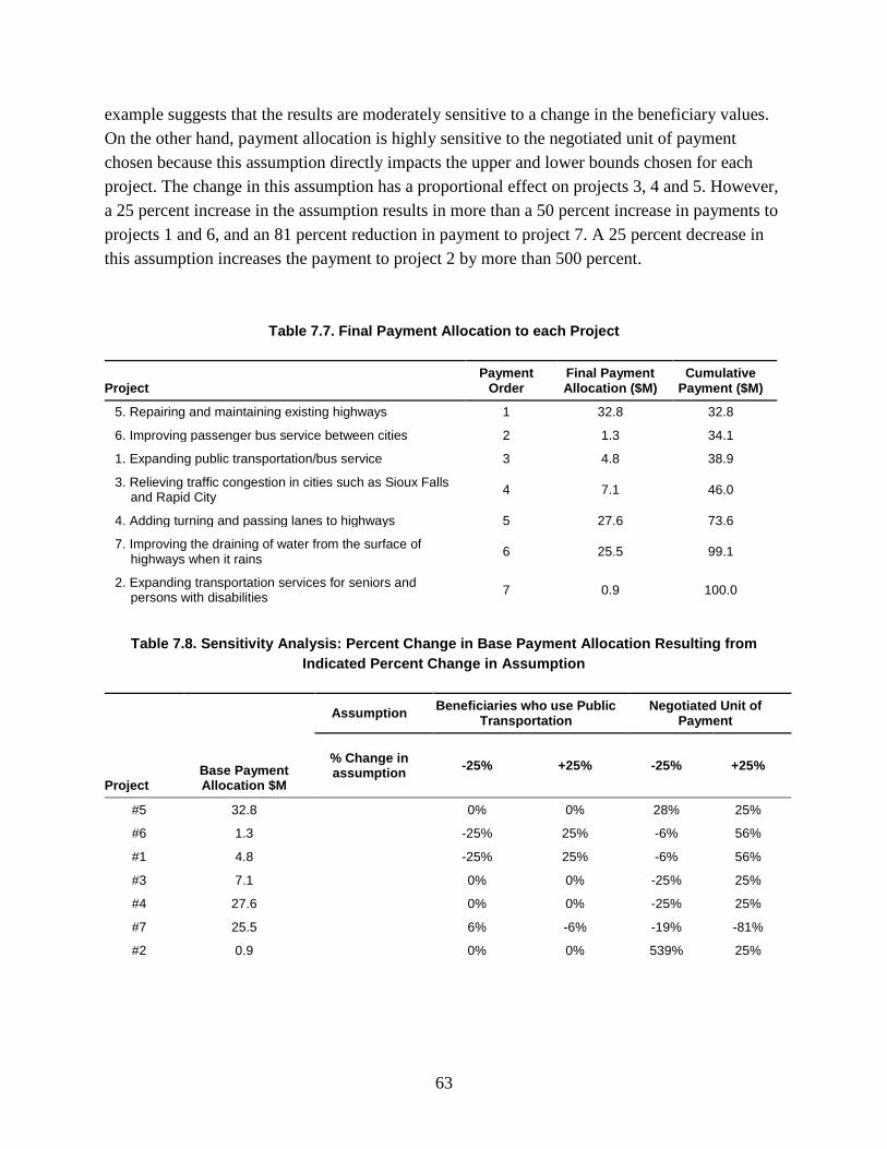
example suggests that the results are moderately sensitive to a change in the beneficiary values. On the other hand, payment allocation is highly sensitive to the negotiated unit of payment chosen because this assumption directly impacts the upper and lower bounds chosen for each project. The change in this assumption has a proportional effect on projects 3, 4 and 5. However, a 25 percent increase in the assumption results in more than a 50 percent increase in payments to projects 1 and 6, and an 81 percent reduction in payment to project 7. A 25 percent decrease in this assumption increases the payment to project 2 by more than 500 percent.

Table 7.7. Final Payment Allocation to each Project

Project Payment

Order Final Payment Allocation ($M)

Cumulative Payment ($M)

5. Repairing and maintaining existing highways 1 32.8 32.8

6. Improving passenger bus service between cities 2 1.3 34.1

1. Expanding public transportation/bus service 3 4.8 38.9

3. Relieving traffic congestion in cities such as Sioux Falls and Rapid City 4 7.1 46.0

4. Adding turning and passing lanes to highways 5 27.6 73.6

7. Improving the draining of water from the surface of highways when it rains 6 25.5 99.1

2. Expanding transportation services for seniors and persons with disabilities 7 0.9 100.0

Table 7.8. Sensitivity Analysis: Percent Change in Base Payment Allocation Resulting from Indicated Percent Change in Assumption

Project Base Payment Allocation $M

Assumption Beneficiaries who use Public Transportation

Negotiated Unit of Payment

% Change in assumption -25% +25% -25% +25%

#5 32.8

0% 0% 28% 25%

#6 1.3 -25% 25% -6% 56%

#1 4.8 -25% 25% -6% 56%

#3 7.1 0% 0% -25% 25%

#4 27.6 0% 0% -25% 25%

#7 25.5 6% -6% -19% -81%

#2 0.9 0% 0% 539% 25%

63

7.5 Advantages and Limitations of DEA, CA, and FDA applications The relative strengths and weaknesses of application of each technique are discussed below.

Accommodating both quantitative and qualitative performance measures

• DEA: In general, DEA requires quantitative measures of each project’s expected inputs and outputs. Though the technique can support qualitative measures as well, inclusion of such measures cannot be done in a straightforward manner, as noted in Section 7.2.

• CA: The evaluation framework applied in the current study includes several qualitative categorical measures (create/support an inclusive community, consistent with local/regional/state plans, and additional protections to water, habitat, and ecosystem). Unlike DEA technique, CA was able to accommodate these performance measures quite easily.

• FDA: The technique cannot accommodate any performance measures.

Accommodating performance measures that may take negative values

• DEA: Additional data manipulation is required to include performance measures that can take on both positive and negative values.

• CA: The current study considers several negative value performance measures, including reduction in VMT, SOV trips, CO2 emission, criteria pollutant emissions, noise level, crashes and fatality rates, and obesity rates among children and adults. The CA technique was able to accommodate these measures without difficulty.

• FDA: The technique cannot accommodate any performance measures, as noted above.

Sensitivity to decision-makers’/stakeholders’ preferences

• DEA: DEA is not sensitive to decision-makers’/stakeholders’ preferences as no input from these groups is required to apply the technique.

• CA: Through the data collected during the survey, decision-makers preferences were directly incorporated into the calculation of the weights associated with each performance measure. Thus, decision-makers’/stakeholders’ understanding of the scale of the decision-making, including the fundamental assumptions applied to design the trade-off exercises, plays a key role in the final weights.

• FDA: Stakeholders’ preferences are one of the key inputs in the FDA process. As a result, the technique is fairly sensitive to stakeholders’ understanding of different types of projects under consideration. This issue may be addressed to a certain extent by surveying a large number of stakeholders.

Ease of implementation: data collection, sample size, and data analysis

• DEA: DEA does not have any strict sample size requirements, but is particularly well-suited to analyses that seek to compare many different alternatives along a relatively select set of attributes. In general, there should be at least two to three times as many alternatives as attributes. As noted earlier, the data should be quantitative rather than qualitative, though categorical attributes can be supported with some additional effort.

64

• CA: This technique involves designing a special survey to collect data on trade-offs between the performance measures. The data from these trade-off exercises are analyzed to estimate the weight of each performance measure. The weights can be estimated using any of several different methods, ranging from a simple count of responses to the different exercises (counting analysis method) to more complex multinomial logit models.

• CA could be data intensive. As observed earlier, it was not possible to obtain consistent estimates of weights because the sample size was too small. One way to overcome this problem is to consider a smaller set of performance measures/attributes. Studies have shown that CA is particularly suitable for analyses with 10 or fewer attributes. Another solution to this problem is to involve more stakeholders.

• FDA: The approach relies on stakeholder survey data, which must be obtained in advance. Furthermore, the inclusion of DOT-level stakeholders in the survey sample is particularly concerning because very few DOT-level stakeholders would be exposed to all of the different types of projects except at the highest/most senior levels of DOT management. As a result, the ability to provide an informed opinion on the survey would require these stakeholders to understand and agree to the assumptions underlying the project information in the survey. This could be a time consuming request for senior level managers.

• In addition, the approach applied in the current study relies on obtaining the number of beneficiaries for each project. We estimated these numbers using readily available U.S. Census data. However, these values likely do not reflect the actual number of people who may benefit from a specific project. These data may be difficult to obtain. Furthermore, defining the scope of exactly who benefits from a project may be a subjective process. Should only people who directly benefit from the project be included (such as those who may drive on a specific highway), or should people with indirect benefits be included (such as, those who may reside in areas circumvented by the highway), or should those with indirect benefits be included but provided with less weight than those with direct benefits? No approach is incorrect, but each requires a set of judgments. Furthermore, our FDA approach requires that a unit of payment per beneficiary be established. While we used an objective measure to assign the unit of payment, the choice of this objective measure is in itself subjective. In assigning both the unit of payment value and beneficiary values, a number of assumptions are needed that could easily bias the results of the analysis. Indeed, our sensitivity analyses showed that the results of the FDA approach were highly sensitive to the unit of payment and moderately sensitive to the beneficiary numbers chosen. Changing these values slightly could alter the allocation of funds.

Ease of implementation: availability of literature, software, and other resources

• DEA: A variety of software solutions exist for performing basic versions of DEA (for example, the Benchmarking package in R mentioned earlier). Though more advanced modeling may require manual coding of the linear program and the use of optimization software, many basic (though still useful) applications of DEA can be performed using these existing tools.

• CA: Application of this technique requires special knowledge of CA survey methods (such as conjoint-based choice survey) and statistical modeling. However, literature

65

describing CA technique and its various applications is widely available. In addition, a number of commercial and open-source CA software packages are readily available.

• FDA: Literature on rules-based and optimization-based FDA methods is readily available. Rules-based FDA methods do not require the use of numerical computational tools and therefore, allow for its implementation without any special expertise, training or special software. Optimization-based methods likely require a programmer to develop code, since the method does not appear to be explicitly supported by existing software. For instance, the Texas Department of Transportation (Gurrola and Taboada, 2011) used Matlab to generate potential solutions when applying optimization-based FDA.

Handling large numbers of projects

• DEA: In general, DEA is able to handle large numbers of projects, but it should be noted this increases the data collection burden on the analyst.

• CA: The technique can be implemented to evaluate any number of projects. However, to assure reliability, CA requires all projects under consideration to be described along the same set of performance measures, which could increase data collection efforts quite significantly.

• FDA: Rules-based FDA involves collecting information on stakeholders’ preferences for each project, which could be a time consuming exercise for a large number of projects. In addition, the method requires estimating numbers of beneficiaries for each project. A properly conducted optimization-based FDA requires significant computer power. For instance, the Texas Department of Transportation (Gurrola and Taboada, 2011) generated a search space of 500 potential solutions for their study. While this solution space was relatively small, an increase in the number of projects or measures used for optimization could increase its size dramatically.

Level of expertise required

• DEA: Performing a DEA analysis requires a certain level of expertise. DEA uses linear optimization to rate the efficiency of each candidate project. Modifying one of the basic DEA formulations to suit a particular problem requires a thorough understanding of linear programming. Furthermore, DEA concepts and terminology are relatively dense. Correctly interpreting the results requires basic familiarity with linear optimization and economic interpretations of efficiency (for example, Farrell efficiencies[1]). Finally, the literature provides many extensions to DEA to address specific challenges, but implementing these extensions may require additional expertise.

• CA: CA involves designing a special survey, which requires a certain level of knowledge and expertise on trade-off exercises. Also, depending on the design of the survey, a certain level of understanding of modeling discrete choices may be necessary.

• FDA: FDA can be applied using a rules-based or optimization-based method. While rules-based FDA methods do not require any special expertise or training, optimization-based methods require special programing skills, as noted above. In the current study, we chose a rules-based FDA method to provide the reader with a comparison between a less complex approach and CA and DEA techniques which require special software, expertise, and training.

66

Flexibility

• DEA: Though the most straightforward DEA models are suitable to address a broad array of situations, the DEA literature offers a rich assortment of alternative formulations that have been developed for special cases. Analysts can select the DEA formulation that best suits their situation. These alternative formulations can support the use of categorical variables, undesirable outputs, and alternative interpretations regarding returns to scale, though they may require greater expertise to implement.

• CA: The weights calculated as part of this study should not be applied to evaluate projects that correspond to any specific geographic location as inputs from a number of DOTs were used to estimate these weights. In general, the weights should be updated if there is any significant change in the size or composition of decision-makers or stakeholders groups.

• FDA: The FDA approach used in this study is based on work presented by Brams (2008) and Brams and Taylor (1994), in a modified version of Divide the Dollar, in which projects rated higher by non-beneficiaries and lower by beneficiaries would be paid first (in terms of order, but not necessarily in terms of amount). The approach rewards the “honesty” of the beneficiary, which in this case is measured by how much the beneficiary underestimates the importance of a project relative to the non-beneficiaries. Brams (2008) and Brams and Taylor (1994) employ this approach in an attempt to control the beneficiaries’ inflation of importance. This overall strategy may or may not suit the needs of DOTs as they are trying to allocate budgets. DOTs could certainly alter this strategy to determine order of payments based on some other criteria.

• This last point, however, reveals the most important advantage and limitation of FDA – that of its flexibility. While DOTs can choose fair division rules from a large set of those available to best meet the needs of allocating their budgets, this customization allows for a level of unchecked subjectivity in the analysis. For instance, after all projects had been paid once, Kiryluk (2011) chose to divide any remaining budget evenly among any project that had not received its upper bound level of funding. DOTs may instead decide to employ Strict Alternative rules, in which payment in a second round would continue in the same order as the first round, or Balanced Alternation rules, in which the ordering of turns is reversed such that the last paid project in the first round is the first to be paid in the second round (Brams 2003). Employing either of these fair division rules instead of dividing the budget evenly as Kiryluk (2011) chose would alter the ultimate budget allocation. Thus, great caution must be taken when choosing the fair division rules for the analysis.

67

Appendix A: A Guide for Interviews with Experts and DOT Practitioners to Aid the Preparation of a Hypothetical Evaluation and Prioritization Plan

This document is to support the Task 2 interviews (preparation of a hypothetical evaluation and prioritization plan) and to help ensure that the information sought by interviewers is consistent and meets the needs of the project. It includes a reminder of the scope of Tasks 2 and 3, and a suggested structure/questionnaire outline for the interviews of both experts and state DOT representatives.

Task 2 Scope: Preparation of a hypothetical evaluation and prioritization plan Task 2 is the preparation of a detailed plan to evaluate and prioritize a set of hypothetical

projects and activities that a state DOT might consider as part of the development of their STIP. The plan, which will be implemented in Task 3 once it has been approved by NCHRP, will focus on the parallel application of the three analytical techniques and a comparison of the results of the prioritization.

The plan will specify:

• The overall concept of the hypothetical case study although it need not be specific to a particular state.

• A selection of possible project types to evaluate and the decision criteria for choosing them.

• The algorithms and techniques that will be used. During the development of the plan, the project team will reach out to, and interview, both

experts in the three techniques, and practitioners at state DOTs. These interviews will help with all aspects of the development of the case study. The state DOTs contacts will focus primarily on states with an already somewhat advanced prioritization process and will cover a range of small, medium and large states. RSG will conduct interviews with state DOT staff, with responsibility for interviewing experts shared between all team members; RAND Europe will conduct interviews with international, and in particular, European based experts; the remainder of the team will focus on North American experts.

Task 3: Implementation of a hypothetical evaluation and prioritization plan Task 3 is the implementation of the plan developed in Task 2. The task will be accomplished

in three phases:

69

• Creation of the project list and associated data describing the various projects and programs. Since the data items required by each of the three techniques vary, the objective of this phase of the task will be to describe the projects completely enough so that they be evaluated using each of the three techniques.

• Application of the three techniques in parallel. • Comparison of the results of each application and development of the technical

memorandum documenting the task. The comparison will identify the relative strengths and weaknesses of the three techniques, including data needs and applications costs for small, medium, and large states.

Expert Interviews The focus of the expert interviews is on discussing:

1. An overview of their experience in applying the technique to transportation and other problems. This includes years of experience by field, reference to publications (if any), etc. This could be a mini technical bio.

2. The details of any applications where the technique was used in transportation project or program prioritization (if applicable) or other similar applications if their work is outside the transportation sector. For example, choose three experiences and collect information on:

a. The type of problems (prioritization, resource allocation, etc.) b. Geographic area c. A brief description of the problem d. Implementation year (if the recommendations were implemented).

3. Theoretic applicability of the technique and the space of problems that can be covered with the technique. For example,

a. Can the technique optimize a set of projects/programs across multiple criteria or just one?

b. What are the limitations in terms of the maximum number of projects/programs and criteria that can be optimized?

c. Can the technique combine qualitative and quantitative measures to a single score?

4. Based on experience, what are the contexts in which the technique has been applied successfully? Where has the technique failed to produce useful outcomes?

5. Based on experience, were the results easy to understand by a wide group of people such as agency staff, management, legislators, and stakeholders? (It may be useful to document the answer in a tabular format.)

6. Probe into the details of successful and less successful applications. Issues around:

a. Data-related issue – How easy/difficult was it to collect the data required to apply the technique?

b. Algorithms used – applicability, limitations c. Staff issues – knowledge, experience d. Institutional barriers (for example, institution did not like the answer, did not use

outcome)

70

e. Resource required – Was success/lack of success down to budget availability?

7. Advice on how the techniques should be best applied, and considerations for a successful application in the context of funding decisions at the program and project/activity level.

a. Recommendations on the algorithms and techniques to use b. Data requirements and data issues to overcome c. Resource requirements in terms of staff time, budget, software d. Level of expertise required to implement the technique e. Approaches to understanding and making use of the results

State DOT Interviews The state DOTs contacts focused primarily on states with an already somewhat advanced

prioritization process and will cover a range of small, medium and large states, for example North Carolina, Minnesota, Oregon, Washington, New Mexico, and Kansas.

The focus of the state DOTs interviews was on discussing:

1. Context of the state

a. What are conflicting priorities faced by the state: i. Urban versus rural priorities.

ii. Mix of transit, freight, and auto based personal travel needs. iii. New infrastructure needs in growth area versus renewal needs in established

areas. iv. Economic development versus sustainability tensions.

b. Approach to: i. Comparing urban versus rural priorities.

ii. Comparing multi-modal alternatives, e.g. comparing the benefits and costs of transit and highway investments – does the state trade off highway improvement and transit improvement projects at a project level or allocated funding by mode at a more aggregate (program) level?

iii. Comparing renewal investment versus new built: how does the state compare the value and importance of maintaining and renewing existing infrastructure against potential new build projects?

iv. Comparing economic development versus sustainability tensions.

2. Project evaluation and prioritization approaches are used in the state:

a. Are there reports or literature that describe them, including details such as algorithms?

b. Details on level of effort, resources, involvement of other stakeholders. c. Issues faced, external criticism of approach.

3. Project data and availability to support the test evaluations:

a. What types of data resources does the state use in project and program prioritization efforts?

71

i. Project database (PSRC is an example. This is a database for all projects that includes project definitions, cost information, and describes the projects along a large set of benefit dimensions that can be used for prioritization purposes.).

ii. Planning GIS system (web-based UPlan software used by Utah Department of Transportation. The UPlan system is designed to facilitate information sharing within an agency, between agencies, and between other stakeholders. The system hosts hundreds of GIS layers, including proposed project alignments, environmental constraints, demographic information, accident data, land use, and travel demand forecasts. It also includes non-geographic data such as presentations, meeting agendas and meeting notes, and assists planners with project prioritization).

b. Can those data be released to the project team for use in the mock evaluation?

4. Practical recommendations for how to improve their evaluation process, where they would most benefit from technical guidance.

72

Appendix B: Performance Measure Levels Used in CA Experimental Design

73

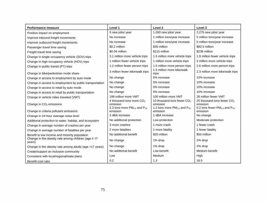
Performance measure Level 1 Level 2 Level 3 Positive impact on employment 5 new jobs/ year 1,000 new jobs/ year 2,275 new jobs/ year

Improve inbound freight movements No increase 1 million tons/year increase 5 million tons/year increase

Improve outbound freight movements No increase 1 million tons/year increase 5 million tons/year increase

Passenger travel time saving $0.2 million $35 million $82.5 million

Freight travel time saving $0.04 million $115 million $238 million

Change in single occupancy vehicle (SOV) trips 3.1 million more vehicle trips 1.5 million more vehicle trips 1.9 million fewer vehicle trips

Change in high occupancy vehicle (HOV) trips 1 million fewer vehicle trips 1 million more vehicle trips 2 million more vehicle trips

Change in public transit (PT) trips 1.2 million fewer person trips 1.5 million more person trips 2.6 million more person trips

Change in bike/pedestrian mode share 3 million fewer bike/walk trips 1.5 million more bike/walk trips 2.3 million more bike/walk trips

Change in access to employment by auto mode No change 5% increase 10% increase

Change in access to employment by public transportation No change 5% increase 10% increase

Change in access to retail by auto mode No change 5% increase 10% increase

Change in access to retail by public transportation No change 5% increase 10% increase

Change in vehicle miles traveled (VMT) 199 million more VMT 100 million more VMT 26 million fewer VMT

Change in CO2 emissions 4 thousand tons more CO2 emission

10 thousand tons fewer CO2 emission

25 thousand tons fewer CO2 emission

Change in criteria pollutant emissions 2.3 tons more PM2.5 and P10 emission

1.2 tons more PM2.5 and P10 emission

0.2 tons fewer PM2.5 and P10 emission

Change in 24-hour average noise level 3 dBA increase 1 dBA increase No change

Additional protection to water, habitat, and ecosystem No additional protection Low protection Moderate protection

Change in average number of crashes per year 3 more crashes 1 more crash 1 fewer crash

Change in average number of fatalities per year 2 more fatalities 1 more fatality 1 fewer fatality

Benefit to low income and minority population No additional benefit $20 million $50 million Change in the obesity rate among children (age ≤ 17 years) No change 1% drop 2% drop

Change in the obesity rate among adults (age >17 years) No change 1% drop 2% drop

Create/support an inclusive community No additional benefit Low benefit Medium benefit

Consistent with local/regional/state plans Low Medium High

Benefit-cost ratio 0.2 1.3 18.5

75

Appendix C: Application of CA and FDA to Non-Transportation Problems

C.1 Conjoint Analysis Applications

Stated Preference Study in Zurich

In this study, the discrete choice modeling (DCM) technique, which is a variant of conjoint analysis, was used to address trade-offs between long-term efficiency investments in two major areas: housing and transport in Canton of Zurich, Switzerland (Jaggi and Axhausen, 2012). A stated preference (SP—the label for the conjoint-type surveys used in transportation applications) survey of homeowners was conducted to understand their energy consumption and related expenses under varying fuel and gas prices across four energy efficient hypothetical alternatives: insulating the house, installing a heat pump, buying more efficient car and switching to public transport or car-sharing. The study is an example of the many hundreds of similar transportation applications that have been conducted using stated preference survey and modeling methods to develop travel choice forecasting models.

Attributes and levels employed for trade-off exercise:

Majority of the attributes are personalized based on individual consumption of car fuel and gas for heating.

5. Investment Costs (CHF): Three absolute lump sum investment levels for insulation of house, installing a heat pump, buy new, more efficient car

6. Gasoline Price (CHF/year): Fixed for all the alternatives in a given scenario, varies with scenario

7. Saving in Mobility costs (CHF/year): Three levels 8. Kilometers driven (CHF/year): Fixed for all the alternatives in a given scenario, varies

with scenario 9. Heating Oil Price (CHF/year): Fixed for all the alternatives in a given scenario, varies

with scenario 10. Saving in heating costs (CHF/year): Three levels 11. CO2 reductions (CHF/year): dependent on the mobility and heating cost reductions

Sample Size:

The SP experiment was based on a design with nine scenarios and is personalized to each individual. A total of 1,088 participants were identified, of which 333 participants fully completed the questionnaire, corresponding to a response rate of 31 percent. In addition to the SP experiment, key socio-economic characteristics, including household income and assets, also were collected in the questionnaire.

76

Types of Models Estimated:

Types of models estimated included basic Multinomial Logit (MNL) models, basic MNL models with additional linear socioeconomic terms (such as expected payback period (PBP), household income effects on investment and fuel prices), and mixed MNL models.

Findings:

From the basic MNL, the PBP (ratio between the parameter for savings and parameter for investment) for insulating the house and heat pump was found to be eight years and five years respectively, and most people were more willing to invest in heat pumps than in insulation. For the car alternatives to reach the same level of utility as a heat pump would require an annual saving of CHF 2,420 and CHF 44,511 for the new car and the car-sharing alternatives respectively.

In the advanced model, a significant PBP (6.5 years) for the insulation alternative was only estimated for people with assets exceeding CHF 150,000 and the PBP for the heat pump that is independent of assets was estimated close to seven years. For the car alternatives to reach same level of utility as a heat pump would require an annual savings of CHF 8,323 and CHF 61,001 for the new car and the car-sharing alternatives respectively.

From the further analysis of the utility trade-offs, it is observed that the decision to invest in a heat pump was dependent on the income level. Investment decisions were dependent on the fuel price and household incomes.

Implementation of the Study Findings:

This study tries to address the problem of understanding homeowners’ investment decisions in energy efficiency with respect to variation in the fuel and gas prices in two different sectors through a SP experiment. However, it remains unclear whether people look at energy consumption as a single entity or divide into the separate budgets depending on the sector. This model still needs to be implemented at an aggregate level and validated as well. Given the spatial and temporal volatility of the fuel and gas prices, the adoption of models of this kind elsewhere needs to be considered carefully.

Denali National Park and Preserve

In this study, stated preference analysis was used to integrate a range of public wilderness values characterized by conditions of social, resource, and managerial attributes of Alaska’s Denali Wilderness into decisions about how to manage the park’s wilderness (Lawson and Manning, 2003a). The study involved collecting data on the choices that overnight wilderness visitors make when faced with hypothetical tradeoffs among the conditions of social, resource, and management attributes of the Denali Wilderness.

77

Attributes and levels employed for trade-off exercise:

Six wilderness setting attributes, each with three levels, were selected to define the social, resource, and management conditions as follows:

Social conditions

1. Number of other groups encountered per day while hiking: 0, 2, or 4+ 2. Able to camp out to camp out of sight and sound of other groups: All nights, most nights,

or a minority of nights.

Resource conditions

1. Extent and character of hiking trails: Hiking is along intermittent animal-like trails, along continuous single-track trails developed from prior human use, or along continuous trails with multiple tracks developed from human use.

2. Signs of human use at camping sites: Little or no signs, some signs, or extensive signs

Management conditions

1. Regulation of camping: Allowed to camp in any zone on any night, required to camp in specified zones, or required to camp in designated sites.

2. Chance of receiving an overnight backcountry permit: Most visitors are able to get a permit for their preferred trip, most visitors are able to get a permit for at least their second choice trip, or only a minority of visitors are able to get a backcountry permit.

Sample size:

Choice based conjoint design was used to prepare four versions of the questionnaire with different attribute-level combination. The survey was administered to overnight visitors at the end of their trip. The participants were randomly assigned a questionnaire and were asked to choose between a pair of alternatives nine times. The final dataset contained information from 311 individuals (an 81.2 percent response rate).

Type of model estimated:

Logistic regression model.

Findings:

The study results provide the Denali Wilderness managers with insight into the relative importance that visitors place on values associated with the wilderness experience and allow managers to predict public support for management alternatives that emphasize those values to varying degrees.

Implementation of study findings:

The findings from this study were incorporated into the 2006 Denali National Park and Preserve Backcountry Management Plan. The plan guides resource protection and visitor use

78

management actions, including administering a permit quota system to manage the number wilderness and backcountry trips per day.

Okefenokee Wilderness

In this study, stated preference analysis was used to examine wilderness preference heterogeneity among different groups of visitors to Georgia’s Okefenokee Wilderness. In particular, the current study examines the choices different groups of visitors make when faced with hypothetical tradeoffs among the wilderness conditions (Lawson et al., 2006).

Attributes and levels employed for trade-off exercise:

Six attributes relevant to the management of the Wilderness was used here. These are:

1. Number of other boats seen per day: 5, 15, and 30+. 2. Cost per day: None, $10/person/day, and $20/person/day. 3. Percentage of water trail miles open to motorboats: 5 percent, 25 percent, 50 percent, and

100 percent. 4. Freedom to enter and travel where you want: Assigned entry point and assigned travel

route, assigned entry point only, assigned travel route only, and no assigned entry point or travel route.

5. Amount of information and education material available to visitors: No information except map, only minimum information (map, simple direction, etc.), and much information

6. Amount of facility development along water routes: No developments, existing a few simple facilities, add a few more facilities.

Sample size:

The stated preference survey was administered to day visitors (both motorized and non-motorized boat users) as well as to overnight wilderness visitors. The visitors were asked to participate in the survey at the end of their trips, and one of the eight versions of the questionnaires was mailed to the visitors who agreed to take the survey. The conjoint part of the questionnaire contained 10 pairwise choice situations, the respondents were asked to choose one alternative from each pair. The final sample included information from 767 visitors (62.2 percent motorized boat, 23.7 percent non-motorized boat, and 14.1 percent overnight visitors).

Type of model estimated:

As indicated earlier, the visitors were divided into three groups: day visitors with non-motorized boats, day visitors with motorized boats, and overnight visitors. Two statistical models were estimated for each group of visitors: a double-censored tobit model and an ordered probit regression model.

79

Findings:

In this study, preference heterogeneity among different groups of visitors to the Okefenokee Wilderness is considered explicitly. The findings from this study suggest that day non-motorized, day motorized, and overnight visitors to the Wilderness do have different preference settings, particularly with respect to how motorboat use of the swamp is managed. However, the results also suggest the visitors groups considered in this study generally share similar preferences for some attributes, such as the number of encounters with other boats and use fees to boat in the swamp.

Isle Royale National Park

In this project, stated preference analysis was used to develop a new wilderness management strategy at Michigan’s Isle Royale National Park. Specifically, a number of prescriptive questions associated with the management of backcountry camping at Isle Royale National Park were examined in this study (for more details, see Lawson and Manning, 2003b).

Attributes and levels employed for trade-off exercise:

The following four attributes, and the corresponding levels, listed below was used to define a number of management scenarios:

1. Percent of groups that share campsites with other people not in their group per night: 0 percent, 5 percent, or 10 percent.

2. Construction of additional campsites: None, or 70 more campsites. 3. Regulations concerning backcountry camping itineraries: Visitors are required to follow

prescribed, fixed itineraries, or no fixed itineraries. 4. The number of permits available to the public: Increased by 10 percent, fixed at current

level, 20 percent reduction, or 75 percent reduction.

Sample size:

Two versions of the questionnaire, each containing 8 pairwise comparisons, were produced, though each respondent was invited to complete only one questionnaire at the end of their camping trip. The participants were asked to choose only one option from each pair of management scenario presented to them. The survey had a 100 percent response rate with 200 completed questionnaires.

Type of model estimated:

Logistic regression model.

Findings:

In this study, visitors were asked to evaluate realistic management alternatives. The results of the analysis provide better understanding of the factors to which visitors are most sensitive in their assessments of management alternatives. For example, study data suggest that restrictive

80

management actions, such as prescribed, fixed itineraries and large reductions in visitor use, are particularly unfavorable to visitors, despite the fact that they are designed to eliminate campsite sharing. Further, the effect of campsite sharing on visitors’ utility is relatively weak. These findings suggest that visitors would prefer to forfeit some degree of campsite solitude to ensure their backcountry camping experiences are relatively free from management control.

Implementation of study findings:

The managers at Isle Royale National Park were faced with value judgments concerning the appropriate balance among public access, visitor freedom, facility development, and camping solitude. The results of this study helped inform the park managers by assisting them in understanding visitor preferences among alternative management scenarios designed to reduce campsite sharing. The study recommendations were included into the 2005 Isle Royale National Park Wilderness and Backcountry Management Plan.

Feasibility of CA as a tool for prioritizing innovations for implementation in UK health care

In this study, CA was used to measure the priorities of healthcare professionals working with women with postnatal depression in a single UK Primary Care Trust (Farley, et al., 2013). Specifically, suitability of the 12 postnatal depression innovations (interventions) being considered as a means of improving the management of the postnatal depression was evaluated based on mapping between the results from a rating based CA exercise and an independent assessment of the attributes in each of the 12 innovations.

Attributes and levels employed for trade-off exercise:

The following seven attributes were identified to be relevant to all the 12 interventions as well-being meaningful to the stakeholders:

1. Impact on care: Low, Limited, Moderate and Significant Improvement 2. Costs: Low, Moderate and High 3. Local health needs: Low Prevalence and High prevalence 4. Minimum standards: Yes and No 5. Strength of supporting evidence: Limited, Moderate and Strong 6. Priority: Local, Local and National. 7. Existence of local expertise: Yes and No

Sample Size:

The CA-based exercise was based on a fraction factorial design with 16 scenarios. This was administered to 1,200 healthcare professionals involved in the care of women with postnatal depression (general practitioners, health visitors, and nurse practitioners) split equally between postal and email delivery methods. To indicate the likelihood of prioritization, participants were asked to rate each of the series of 16 hypothetical innovations on a seven point Likert-type scale

81

anchored at “very likely to prioritize this guideline” through to “very unlikely to prioritize this guideline.” The questionnaire was completed by 11 percent (N = 139) of the sample, with an equal number of responses from postal and email delivery methods.

Types of Models Estimated:

Responses from the CA questionnaire were analyzed using ordinary least square regression with the dependent variable being the priority associated with an innovation and innovation attributes at their component levels as the independent variables. This analysis produced utilities for each attribute and for each level of the attributes. In order to unite this preference data with the independent assessment of attributes in the innovations, the utilities for each attribute at various levels are summed for each individual respondent corresponding. The option with the highest mean utility in the sample represents the “first choice” and thus the most favored.

Findings:

The analysis from this study was helpful in understanding the importance of the attributes of innovations and their importance at various levels and provided a ranked picture of innovations according to the preferences of the people involved in having to implement them. For example, “impact on care” and “strength of evidence” were the top most-prioritized attributes and innovations showing a better improvement in quality of care with supporting evidence, therefore tend to be ranked higher and can be prioritized first.

Implementation of the Study Findings:

This study addresses the problem in the conventional methods of prioritization which are often based on the socio-political factors resulting in bias towards stakeholder groups having higher weight by showing that the preferences can be mapped, matched to innovation characteristics and can be used to shape the design and implementation of interventions to change behavior and encourage adoption. The authors also suggest that though a rating based CA exercise was preferred in this context, Discrete choice experiments (DCE) offer another alternative in which the respondents are faced with direct choice situations. This approach more closely reflects the real decision-making process than CA.

Application of discrete choice modeling (DCM) to clinical service developments in Scotland

This study explores the use of DCM to elicit views of planners of health care, providers of health care and consumers in the area of priority setting (Farrar et al., 2000). Specifically, it shows how the DCM technique can be applied to assist in the process of priority-setting on problems that health care providers face in the context of choosing an appropriate clinical service development from a set of 38 potential clinical service developments proposed by the clinical directors in a hospital in Scotland. In addition to the DCM exercise undertaken by the hospital

82

consultants, the study involved clinical directors who provided scores for attributes for each of the 38 potential clinical service developments.

The coefficients estimated for each attribute from the DCM model are then used as weights to the scores provided by the clinical directors to compute a total weighted score. Cost data were then used to arrive at a cost per unit of benefit ratio for each of the proposed clinical development alternatives. To select the optimal combination of clinical service developments within a given budget, the authors propose Integer programming techniques.

Attributes and levels employed for trade-off exercise:

The following five attributes were identified to be relevant based on discussions with the Members of the Trust Medical Advisory Committee (TMAC):

1. Level of evidence of clinical effectiveness: 3 levels i.e., Requires at least one randomized controlled trial, requires availability of well conducted clinical studies and requires evidence from expert committees.

2. Size of health gain: Small, Large and Medium 3. Contribution to professional development: No change, Improvement 4. Contribution to education training and research: None, 1, 2 and 3 5. Strategy area: No Priority, Local or National Priority, Local and National Priority

Sample Size:

The DCM was based on a design with 16 scenarios giving a total of eight pairwise choices. The respondents were asked to select either of the pairwise choices. A response rate of 60 percent was achieved from a total of 216 consultants working with the hospital who were asked to complete the questionnaire.

Types of Models Estimated:

Random effects probit model

Findings:

The cost per unit of benefit for each development provides the policymakers with evidence on which projects to prioritize in the presence of budget constraints. Integer programming techniques can be applied to arrive at an optimal combination of developments.

Implementation of the Study Findings:

This study provides an application where discrete choice modeling can be used as a potential tool for priority setting by taking into account the views of people primarily involved in implementation of the policies. This also could be extended by taking into account the views of different groups and incorporating them into an economic evaluation framework.

83

C.2 FDA Applications

Water Distribution in Kabylia, Algeria

In this study, fair division analysis was used to determine a water management solution that would lead to an equitable and economical water distribution schedule (namely, the distribution of water over a period of time) for the rural area within the region of Kabylia, Algeria, taking into account a number of physical and engineering constraints (Udias et al., 2012). The study involved developing a set of models, which could then be optimized to achieve maximized equity and minimized costs, including: (1) a portion of the water distribution network in Kabylia, (2) the daily per capita demand as a function of time and (3) the energy costs related to pumping the water.

Objective Function/Decision Criteria or Rules:

A bicriteria fair division problem was modeled based on the objectives of:

• Maximizing equity, as measured by the per capita water deficit over time and the balance of the water deficit over time among all inhabitants (consumption points

in the distribution network) • Minimizing costs, which is a function of the energy costs related to pumping the water.

Type of FDA methods used:

• Optimization Based

Findings:

The Spanish Cooperation and Development Agency supported this study to find alternative water management solutions to the current policy, which had been found to cause an inequitable distribution of water across the rural villages in Kabylia.

Implementation of study findings:

The study highlighted a number of alternative water management solutions that, when compared to the current management policy, could reduce costs while providing a more equitable distribution of water to the villages. The solutions included different improvements to certain infrastructures in the water distribution network. The study also illustrated the difficulty with guaranteeing an equitable supply in the network when small increases in demand arise or when problems occur with the network facilities.

Water Distribution in Alberta, Canada

In this study, fair division analysis was used to determine a fair and efficient water allocation solution among competing users for South Saskatchewan River Basin in southern Alberta, Canada, assuming a public water rights regime (Hipel et al., 2013). The study involved

84

developing a set of models, which could then be optimized to maximize equity and efficiency, and was based on systems level thinking, along with the integration of hydrologic, environmental, societal and economic considerations.

Objective Function/Decision Criteria or Rules:

A fair division problem was modeled using an overall river basin systems model with the following decision rules:

• A priority ranking among domestic water demands and commercial and industrial water demands.

• Minimizing the water shortage ratios across all demands. • Minimizing the differences among all water shortages.

Type of FDA methods used:

• Optimization-based

Findings:

When compared to the status quo (private ownership of all water rights), modeling allocation under a public water rights regime shows that in wet and normal hydrologic years, nearly all water demands can still be satisfied. Under drought cases, the results produce relatively evenly distributed water allocations that are still economically efficient.

Implementation of study findings:

The study highlighted how a public water rights regime, when modeled with FDA, could still equitably and efficiently allocate water rights when compared to the current management policy.

Assignment of Software Engineering Projects

In this study, fair division analysis was used to openly and equitably apportion the tasks of a software engineering project among four undergraduate student teams in a software engineering course at Missouri’s Truman State University (Beck, 2008). The study involved the use of a sealed-bid auction on four tasks of the project in which each team was given 100 points to bid on the tasks. The bidding was meant to correctly portray each team’s valuation of each task relative to the others. An algorithm was then used to assign a task to each team that was relatively desirable, while at the same time trying to minimize disparity among the teams’ awards.

Objective Function/Decision Criteria or Rules:

Once sealed bids were elicited for a task, an algorithm was used to satisfy the following objectives:

• Task assigned to each team should be (somewhat) desirable to that team, relative to the other tasks.

85

• Minimize the disparity among each team’s award task, defined as the sum of the differences between the team’s sealed bid value of that task and a “fair value” of the task of 25 points.

• Minimize the difference in disparity between teams. Providing bonus points toward the teams’ grades that was proportional to the disparity

equalized the remaining disparity of each team.

Type of FDA methods used:

Rules-based and Optimization-based methods (modification to Knaster’s procedure of sealed bids – see section 4.1 for an explanation of this method).

Findings:

Over five years, the author has been using this method in his classroom and each time has been able to find a solution that students deemed fair. Teams awarded a task of relatively lesser value were provided bonus points to provide an envy-free and equitable solution.

Implementation of study findings:

The study applied a modification of Knaster’s procedure of sealed bids to allocate a set of indivisible goods. The method simplifies Knaster’s procedure by apportioning the number of tasks to be equal to the number of teams.

The Winsor Family Silver

In this study, fair division analysis was used to equitably divide an inheritance of silver items, each having differing monetary and sentimental value, among eight grandchildren of the deceased owner (Pratt and Zeckhauser 1990). The study involved eliciting the grandchildren’s utilities for each item. These utilities were used to buy probability shares in the items within a pseudo-market in which each grandchild had equal endowment in an artificial currency. The shares were used in a lottery, which assigned items to the grandchildren in accordance with the probability shares.

Objective Function/Decision Criteria or Rules:

Once utilities were elicited for each silver item, equilibrium prices could be calculated for each item using the following rules:

• If only one grandchild desired an item, it went to them at no cost to their artificial currency.

• For the remaining contended items, the budget of a grandchild who wanted only one contended item would be spent entirely on that item.

• A “see if you can work it out” allocation method of remaining items was employed based on a mechanism developed by Hylland and Zeckhauer (1979) that calculates indifference prices within a set of constraints to reach equilibrium.

86

Type of FDA models/methods used:

Rules-based and Optimization-based method (pseudo market-based approach developed by Hylland and Zeckhauer (1979)).

Findings:

As one of the grandchildren involved, Pratt (first author of the study) was trusted by his relatives to find a fair and understandable mechanism to divide the Winsor family silver. Pratt conducted utility elicitations of each grandchild, which enabled the (perceived) equitable distribution of the silver.

Implementation of study findings:

The study applied a pseudo-market rules-based method, as well as an optimization-based method, to allocate a set of indivisible goods. The outcome of this method only produces an efficient result within the constrained world set up with the artificial currency. The fairness of the method is based on its offering of equal endowments and symmetric opportunities.

The Pope Family Furniture and Household Items

In this study, fair division analysis was used to equitably divide an inheritance of furniture and household items, each having differing monetary and sentimental value, among two children and 13 grandchildren of the deceased owner (Nickolaus 2012). The study compares the allocation of this inheritance using a complex fair-division procedure (“the Pope Procedure”), as well as other frequently used procedures. The Pope Procedure involved eliciting the participants’ ranked preferences for as many items as they wished, as well as assigning fair-market value for each item.

Objective Function/Decision Criteria or Rules:

Once rankings were elicited for each item, an auction mechanism was conducted using the following rules:

• If only one participant ranked an item as best, it went to them at the fair market cost. • Ties in best ranking were handled last, with the overall number of items already assigned

to each individual determining the outcome. • Proceeds from the procedure were divided in accordance with the rule for dividing the

cash value of the remainder of the estate.

Type of FDA models/methods used:

Rules-Based Method (loosely based on the Alternation Procedure - other allocation approaches described in the study include Knaster’s Sealed Bids and Adjusted Winner)

87

Findings:

Of the procedures considered (including the Pope Procedure), only Knaster’s Sealed Bids and one version of the Adjusted Winner approach achieved proportionality given the preferences of the Pope Family. Envy-Freeness was achieved under most approaches, including the Pope Procedure. Equitability was not achieved by any mechanism except for a version of the First Price Auction. All mechanisms other than the Pope Procedure and Adjusted Winner attain efficiency.

Implementation of study findings:

The study applied an approach based loosely on the Alternating Procedure to allocate a set of indivisible goods. The Pope family chose this approach because they wanted one that would produce an envy-free result with financial fairness. In light of their priorities, the Pope Procedure seemed to do a relatively good job of matching the criteria most valued by the Pope family. The allocation was envy-free, gave each participant his or her first choice item, and respected the financial constraints affecting some family members.

Budget allocation for the European Union’s rural-development policy in Poland

In this study, the effectiveness of a fair-division algorithm when applied to a practical structural policy budget allocation problem for a case of the EU’s rural-development policy budget in Poland (Kiryluk, 2013) is evaluated. The specific objectives of the EU’s rural development program are improving the competitiveness of agriculture and forestry, improving the environment and the countryside, and improving the quality of life in rural areas. The multi-objectivity of the program diversity of the proposed measures raise many conflicts in priority setting among potential beneficiaries and country-level decision-makers. Poland had selected 18 measures under the three main objectives and a budget of €15.24 billion was allocated to implement these measures. The study involved a survey of the key stakeholders: farmers (beneficiaries), experts and farmer advisers. It also involved quantifying the preference for a given measure on a scale of 1 (low impact) to 9 (high impact). To allocate the budget in a reasonable way, pre-defined upper and lower bounds for each measure are derived. Brams and Taylor’s Algorithm was then used to determine the order of payment and pay-off for each measure.

Objective Function/Decision Criteria or Rules:

A framework for budget- allocation procedure based on Brams and Taylor’s algorithm is adopted using the following approach:

• Standardization of all the three stakeholder preferences for the 18 identified measures. • Defining restrictions for the budget allocation payoff scheme.

− The upper bound is objectively calculated taking into account two variables:

88

Pre-negotiated and fixed by the EU unit support for each measure. Size of the targeted group of beneficiaries that meet the program’s eligibility

criteria. − The lower bound is the higher of the amount of the previous commitment or 10

percent of the upper bound of the measure.

• Budget allocation using FD algorithm

− Determine the order of payments, i.e., which measure needs to be paid first. − Determine the specific budgets for each of the measure using a pay-off table.

Type of FDA methods used:

Rule-based

Findings:

When compared with the actual allocation, fair-division algorithms assign more funds to the measures that are highly rated by all of the stakeholder groups.

Implementation of study findings:

This study demonstrates that implementing FDA algorithms is feasible and leads to reasonable solutions that are arguably superior to less formal methods currently used by decision-makers for solving complex budget allocation problems that involve multiple competing measures and stakeholder groups.

Resolving an Italian insurance allocation problem

In this study, the problem of the determination of a fair allocation in a co-insurance problem, such as how insurance companies have to share risk. The premium is studied and a procedure to produce a proportional and an equitable allocation is proposed and applied in a real situation to a pool of 61 insurance companies in Italy that have the responsibility for environmental pollution risks (Ambrosino et al., 2006). The study involved investigations of efficient allocations under in accordance with proportionality and equality, which are not obtained by the widely used quota share allocation methods for sharing risk and premium.

Objective Function/Decision Criteria or Rules:

A formal description of the problem in Fragnelli and Marina, 2003 is used: • Each company submits, independently its function for evaluating risks to a mediator who

selects an optimal decomposition for that risk. • Each company receives an equal share of the total premium. • Each company pays a quota of risk according to its evaluation. • Companies receive a refund based on the difference between their own evaluation of the

risk and the optimal decomposition.

89

• The surplus, if shared equally among all the companies, leads to a proportional allocation and if the surplus is shared among all the companies proportional to their net profit, then it leads to an equitable allocation.

Type of FDA methods used:

Rules-Based and optimization methods based on Knaster’s procedure.

Findings:

The results from the two allocations proposed in this work are a good compromise between a quota share allocation and the envy-free allocation. The equitable allocation is also proportional and is therefore the best choice that a mediator may propose.

Implementation of study findings:

This study demonstrates an application of fair division methods that can provide solutions of suitable bargaining problems and outputs of mediation procedures in a negotiation.

90

References

Ambrosino, Daniela, Vito Fragnelli and Maria E. Marina, “Resolving an insurance allocation problem: a procedural approach.” Social Choice and Welfare Vol. 26, April 4, 2006, pp. 625-643. As of December 15, 2014: http://www.jstor.org/discover/10.2307/41106755?uid=3739256&uid=2&uid=4&sid=21105461082093

Banker, R., A. Charnes and W.W. Cooper, “Some models for estimating technical and scale inefficiencies in data envelopment analysis.” Management Science Vol. 30, No. 9, September 1984, pp. 1078-1092. As of December 15, 2014: http://astro.temple.edu/~banker/DEA/13%20Some%20Models%20for%20Estimating%20Technical%20and%20Scale%20Inefficiencies.pdf

Barnum, Darold T., Sue McNeil, Jonathan Hart, “Comparing the Efficiency of Public Transportation Subunits Using Data Envelopment Analysis,” Journal of Public Transportation, Vol. 10, No. 2, 2007. As of December 15, 2014: www.nctr.usf.edu/jpt/pdf/JPT%2010-2%20Barnum.pdf

Beck, Jon, “Fair division as a means of apportioning software engineering class projects.” ACM SIGCSE Bulletin, 2008, pp. 68-71. As of December 15, 2014: http://www.researchgate.net/publication/221538585_Fair_division_as_a_means_of_apportioning_software_engineering_class_projects

Boame, Attah K., “The technical efficiency of Canadian urban transit systems.” Transportation Research Part E: Logistics and Transportation Review, Vol. 40, Issue 5, September 2004. p. 401. As of December 15, 2014: http://www.sciencedirect.com/science/article/pii/S1366554503000784

Böhringer, Christoph, and Carsten Helm, “On the fair division of greenhouse gas abatement cost,” Resource and Energy Economics, Vol. 30, No. 2, May 2008, pp. 260-276. As of December 16, 2014: http://www.sciencedirect.com/science/article/pii/S0928765507000425

Brams, Steven J., “Fair Division,” The Encyclopedia of Public Choice, 2003, pp. 572-574. As of December 16, 2014: http://link.springer.com/chapter/10.1007%2F978-0-306-47828-4_103

------ , “What do you think you’re worth?” Plus, March 1, 2008. As of December 16, 2014: http://plus.maths.org/content/what-do-you-think-youre-worth

Brams, Steven J., and Alan D. Taylor, “Divide the dollar: Three solutions and extensions,” Theory and Decision Vol. 37, Issue 2, September 1994, pp. 211-231. As of December 16, 2014: http://link.springer.com/article/10.1007%2FBF01079266

91

------, Fair Division: From Cake-Cutting to Dispute Resolution. Cambridge: Cambridge University Press, 1996.

------, The Win-Win Solution: Guaranteeing Fair Shares to Everybody. New York: W.W. Norton & Company, 1999.

Caulfield, Brian, Diarmuid Bailey and Shane Mullarkey, “Using data envelopment analysis as a public transport project appraisal tool,” Transport Policy, Vol. 29, September 2013, pp. 74-85. As of December 16, 2014: http://www.sciencedirect.com/science/article/pii/S0967070X13000577

Charnes, A., W. W. Cooper, and Edwardo L. Rhodes, “Measuring the efficiency of decision making units,” European Journal of Operational Research Vol., 2, Issue 6, November 1978, pp. 429-444. As of December 16, 2014: http://www.sciencedirect.com/science/article/pii/0377221778901388

Cooper, William W., Lawrence M. Seiford, and Kaoru Tone. Data Envelopment Analysis: A Comprehensive Text with Models, Applications, References and DEA-Solver Software (2nd Edition). New York: Springer, 2007.

Damarat, Sebastian, and Bernard Roy, “The uses of cost-benefit analysis in public transportation decision-making in France,” Transport Policy, Vol. 16, Issue 4, August 2009, pp. 200-212.

DisabilityPlanningData.com, “Disability Population Statistics for South Dakota From Pooled 2005-2007.” As of December 16, 2014: http://disabilityplanningdata.com/site/state_population_table.php?state=southdakota

Farley, Katherine, Carl Thompson, Andria Hanbury, and Duncan Chambers, “Exploring the feasibility of Conjoint Analysis as a tool for prioritizing innovations for implementation,” Implementation Science, Vol. 8, No. 56, May 2013. As of December 16, 2014: http://www.implementationscience.com/content/8/1/56

Farrar, Shelley, Mandy Ryan, Donald Ross, Anne Ludbrook, “Using discrete choice modeling in priority setting: an application to clinical service developments,” Social Science & Medicine, Vol. 50, Issue 1, January 2000, pp. 63-75. As of December 16, 2014: http://www.sciencedirect.com/science/article/pii/S0277953699002683

Fernandes, Elton, and R. R. Pacheco, “Efficient use of airport capacity,” Transportation Research Part A: Policy and Practice, Vol. 36, Issue 3, March 2002, p. 225. As of December 16, 2014: http://www.sciencedirect.com/science/article/pii/S096585640000046X

Gühnemann, Astrid, James J. Laird, and Alan D. Pearman, “Combining cost-benefit and multi-criteria analysis to prioritise a national road infrastructure programme,” Transport Policy, Vol. 23, September 2012, pp. 15-24. As of December 16, 2014: http://www.sciencedirect.com/science/article/pii/S0967070X12000753

92

Gurrola, Emmanuel, and Heidi A. Taboada, “A Sequential Fund Allocation Approach to Minimize Envy,” Proceedings of the 41st International Conference on Computers & Industrial Engineering, Los Angeles, 2011. As of December 16, 2014: http://www.usc.edu/dept/ise/caie/Checked%20Papers%20%5Bruhi%…AL%20FUND%20ALLOCATION%20APPROACH%20TO%20MINIMIZE%20ENVY.pdf

Hipel, Keith W., Liping Fang, and Lizhong Wang, “Fair water resources allocation with application to the south Saskatchewan river basin,” Canadian Water Resources Journal, Vol. 38, No. 1, 2013, pp. 47-60. As of December 16, 2014: http://www.tandfonline.com/doi/abs/10.1080/07011784.2013.773767#.VJCTmieNXJw

Hylland, Aanund, and Richard Zeckhauser, “The efficient allocation of individuals to positions,” The Journal of Political Economy, Vol. 87, Issue 2, 1979, pp. 293-314. As of December 16, 2014: https://ideas.repec.org/a/ucp/jpolec/v87y1979i2p293-314.html

Ijzerman, Maarten J., Janine A. Van Til and John F.P. Bridges, “A Comparison of Analytic Hirerachy Process and Conjoint Analysis Methods in Assessing Treatment Alternatives for Stroke Rehabilitation,” The Patient - Patient-Centered Outcomes Research, Vol. 5, Issue 1, March 2012, pp. 45-56. As of December 16, 2014: http://link.springer.com/article/10.2165/11587140-000000000-00000?no-access=true

Ivanović, Ivan, Dragana Grujićić, Dragana Macura, Jadranka Jović, Nebojsa Bojović, “One approach for road transport project selection,” Transport Policy Vol. 25, January 2013, pp. 22-29. As of December 16, 2014: http://www.sciencedirect.com/science/article/pii/S0967070X12001588

Jaggi, B. and Axhuasen, K.W. (2012) Modeling Long Term Investment Decisions in Housing and Transportation, Working paper, 840, Institute of Transport Planning and Systems (IVT), ETH Zurich, Zurich.

Kiryluk-Dryjska, Ewa, “Fair Division Approach for the European Union’s Structural Policy Budget allocation: An Application Study,”Group Decision and Negotiation, Vol. 23, Issue 3, March 16, 2013. As of December 16, 2014: http://link.springer.com/article/10.1007%2Fs10726-013-9346-6

Knaster, Bronislaw, “Sur le probleme du partage pragmatique de H. Steinhaus,” Annales de la Societe Polonaise de Mathematique Vol. 19, 1946, pp. 228-230.

Lawson, Steven, Joseph W. Roggenbuck Troy E. Hall, and Aurora Moldovanyi, “A conjoint analysis of preference heterogeneity among subgroups of Okefenokee Wilderness visitors,” Journal of Leisure Research, Vol. 38, Issue 4, pp. 575-600. As of December 16, 2014: https://www.questia.com/library/journal/1G1-155751036/a-conjoint-analysis-of-preference-heterogeneity-among

93

Lawson, Steven R., and Robert Manning, “Integrating multiple wilderness values into a decision-making model for Denali National Park and Preserve,” Journal for Nature Conservation 2003, pp. 355-362. As of December 16, 2014: http://www.sciencedirect.com/science/article/pii/S1617138104700679

-------, “Research to guide management of backcounty camping at Isle Royale National Park: Part II – Prescriptive research,” Journal of Park and Recreation Administration, Vol. 21, Issue 3, 2003, pp. 43-56. As of December 16, 2014: http://js.sagamorepub.com/jpra/article/view/1498

McFadden, Daniel, “The Revealed Preferences of a Government Bureaucracy: Empirical Evidence,” The Bell Journal of Economics, Vol. 7, No. 1, Spring 1976. As of December 16, 2014: http://www.jstor.org/discover/10.2307/3003190?sid=21105468180223&uid=4&uid=2&uid=3739256

Nickolaus, Cara, and R. Cytron, “Fair Division of an Inheritance: A Case Study,” Washington University of St. Louis paper, fall 2012. As of December 16, 2014: http://www.cs.wustl.edu/~cytron/cake/Reports/PDFs/caranickolaus.pdf

Nolan, J. F., P. C. Ritchie, and J. E. Rowcroft, “Identifying and measuring public policy goals: ISTEA and the US bus transit industry,” Journal of Economic Behavior & Organization, Vol. 48, Issue 3, p. 291. As of December 16, 2014: https://ideas.repec.org/a/eee/jeborg/v48y2002i3p291-304.html

Outwater, Maren L., Thomas Adler, Jeffrey Dumont, Matthew Kitchen and Alon Bassok, “Quantitative Approaches for Project Prioritization: Case Study in Puget Sound,” Washington, D.C.: Journal of the Transportation Research Board, No. 2303, 2012, pp. 108-116. As of December 16, 2014: http://trid.trb.org/view.aspx?id=1128692

Pratt, John Winsor, and Richard Jay Zeckhauser, “The fair and efficient division of the Winsor family silver,” Management Science, Vol. 36, No. 11, 1990, pp. 1293-1301. As of December 16, 2014: http://econpapers.repec.org/article/inmormnsc/v_3a36_3ay_3a1990_3ai_3a11_3ap_3a1293-1301.htm

Rawls, John. A Theory of Justice. Cambridge, Mass.: Belknap Press, 1971.

Robertson, Jack, and William Webb. Cake-Cutting Algorithms: Be Fair If You Can. Natick, Mass.: A K Peters/CRC Press, 1998.

Saaty, T.L. The Analytic Hierarchy Process. New York: McGraw-Hill, 1980.

94

South Dakota Department of Transportation “SDDOT 2011 Statewide Customer Satisfaction Assessment,” SD2010-03, January 2012. As of December 16, 2014: http://www.sddot.com/business/research/projects/docs/SD2010-03_FinalReport_Oct17.pdf

Steinhaus, Hugo, “The problem of fair division,” Econometrica, Vol. 16, No. 1, 1948, pp. 101-104.

-------, “Sur la division pragmatique,” Econometrica: Journal of the Econometric Society, 1949, pp. 315-319.

Suzuki, Soushi, Peter Nijkamp, Eric Pels and Piet Rietveld, “Comparative performance analysis of European airports by means of extended data envelopment analysis,” Journal of Advanced Transportation, Vol 48, Issue 3, April 2014. As of December 16, 2014: http://onlinelibrary.wiley.com/doi/10.1002/atr.204/abstract

Tax Policy Center, “State and Local Tax Revenue, Per Capita,” September 20, 2013. As of December 16, 2014: http://www.taxpolicycenter.org/taxfacts/displayafact.cfm?Docid=513

Tsamboulas, Dimitrios A., “A tool for prioritizing multinational transport infrastructure investments,” Transport Policy, Vol. 14, Issue 1, pp. 11-26. As of December 16, 2014: http://www.sciencedirect.com/science/article/pii/S0967070X06000576

Turner, Hugh, Robert Windle, and Martin Dresner, “North American container port productivity: 1984-1997.” Transportation Research Part E: Logistics and Transportation Review, Vol. 40, Issue 4, July 2004, p. 339. As of December 16, 2014: http://www.sciencedirect.com/science/article/pii/S1366554503000760

Udías, Angel, David Rios Insua, Javier Cano, and Hocine Fellag, “Cost-efficient equitable water distribution in Algeria: A bicriteria fair division problem with network constraints,” International Transactions in Operational Research, Vol. 19, No. 5, April 2012, pp. 675-693. As of December 16, 2014: http://onlinelibrary.wiley.com/doi/10.1111/j.1475-3995.2012.00846.x/abstract

United We Ride, “South Dakota; United We Ride Report,” 2007. As of December 17, 2014: http://www.unitedweride.gov/United_We_Ride_Report_and_Action_Steps_-_South_Dakota_8-30-07.pdf

U.S. Census Bureau, “State and County QuickFacts, South Dakota.” As of December 17, 2014: http://quickfacts.census.gov/qfd/states/46000.html

U.S. Census Bureau (2014b); generated by Lauren Mayer; using CensusExplorer, Population Estimates Edition. As of September 3, 2014: http://www.census.gov/censusexplorer/censusexplorer-popest.html.

-------, “State and County QuickFacts, Sioux Falls (city), South Dakota.” As of December 17, 2014: http://quickfacts.census.gov/qfd/states/46/4659020.html

95

--------, “State and County QuickFacts, Rapid City (city), South Dakota.” As of December 17, 2014: http://quickfacts.census.gov/qfd/states/46/4652980.html

Xuehao, Chu, Gordon J. Fielding, and Bruce W. Lamar, “Measuring transit performance using data envelopment analysis,” Transportation Research. Part A: Policy and Practice, Vol. 26, Issue 3, May 1992, pp. 223-230. As of December 17, 2014: http://www.sciencedirect.com/science/article/pii/0965856492900334

96