NBER WORKING PAPER SERIES

THE PUZZLE OF THE ANTEBELLUM FERTILITY DECLINE IN THE UNITED STATES:NEW EVIDENCE AND RECONSIDERATION

Michael R. HainesJ. David Hacker

Working Paper 12571http://www.nber.org/papers/w12571

NATIONAL BUREAU OF ECONOMIC RESEARCH1050 Massachusetts Avenue

Cambridge, MA 02138October 2006

The views expressed herein are those of the author(s) and do not necessarily reflect the views of theNational Bureau of Economic Research.

© 2006 by Michael R. Haines and J. David Hacker. All rights reserved. Short sections of text, notto exceed two paragraphs, may be quoted without explicit permission provided that full credit, including© notice, is given to the source.

The Puzzle of the Antebellum Fertility Decline in the United States: New Evidence and ReconsiderationMichael R. Haines and J. David HackerNBER Working Paper No. 12571October 2006JEL No. J1,J13,N21,N3

ABSTRACT

All nations that can be characterized as developed have undergone the demographic transition fromhigh to low levels of fertility and mortality. Most presently developed nations began their fertilitytransitions in the late nineteenth or early twentieth centuries. The United States was an exception. Evidence using census-based child-woman ratios suggests that the fertility of the white populationof the United States was declining from at least the year 1800. By the end of the antebellum periodin 1860, child-woman ratios had declined 33 percent. There is also indication that the free black populationwas experiencing a fertility transition. This transition was well in advance of significant urbanization,industrialization, and mortality decline and well in advance of every other presently developed nationwith the exception of France. This paper uses census data on county-level child-woman ratios to testa variety of explanations on the antebellum American fertility transition. It also uses micro data fromthe IPUMS files for 1850 and 1860. A number of the explanations, including the land availabilityhypothesis, the local labor market-child default hypothesis, and the life cycle saving hypothesis, areconsistent with the data, but nuptiality, not one of the usual explanations, emerges as likely very important.

Michael R. HainesDepartment of Economics, 217 Persson HallColgate University13 Oak DriveHamilton, NY 13346and NBERMHAINES@MAIL.COLGATE.EDU

J. David HackerDepartment of HistoryBinghamton University (SUNY)PO Box 6000Binghamton, NY 13902hacker@binghamton.edu

2

INTRODUCTION

All nations that can be characterized as developed have undergone the demographic

transition from high to low levels of fertility and mortality. Most presently developed nations

began their fertility transitions in the late nineteenth or early twentieth centuries [Coale and

Watkins, 1986, ch. 1]. The United States was an exception. Evidence using census-based child-

woman ratios suggests that the fertility of the white population of the United States was declining

from at least the year 1800. By the end of the antebellum period in 1860, child-woman ratios had

declined 33 percent. There is also indication that the free black population was experiencing a

fertility transition. This transition was well in advance of significant urbanization,

industrialization, and mortality decline and well in advance of every other presently developed

nation with the exception of France. Therein lies the puzzle.

Unfortunately, attempts to solve the puzzle of early American fertility decline are hampered

by a lack of reliable data. Our most comprehensive source of fertility data is census-based child-

woman ratios. While having the virtue of being highly correlated with total fertility and being

easily constructed at the state and county level for the white population between 1800 and 1860,

child-woman ratios present significant liabilities for the study of fertility decline. One problem is

their sensitivity to mortality. Two counties with identical levels of fertility and different levels of

mortality will have different child-woman ratios, the county with the highest mortality having the

lowest child-woman ratio. The bias can be severe. Indeed, new evidence suggests that a significant

part of the national decline in child-woman ratios between 1800 and 1860 was due to increasing

mortality [Hacker, 2003]. We know little about regional and urban/rural differentials in antebellum

mortality, but it is likely that some of the observed geographic differentials in child-woman ratios

reflect differential mortality. A second problem with child-woman ratios is their inability to

3

distinguish the relative contribution of nuptiality (the timing and incidence of marriage) and marital

fertility (fertility rates within marriage) to overall fertility. Despite these liabilities, however,

economic historians have constructed elaborate theories of U.S. fertility decline that emphasize the

importance of fertility control within marriage. Complex neo-Malthusian mechanisms are stressed

when simple Malthusian explanations may do.1

This paper uses improved source data to test various theories of U.S. antebellum fertility

decline. In the first part of the analysis, we rely on child-woman ratios and other county-level

aggregate data from the population and economic censuses of 1800 to 1860 and the agricultural and

manufacturing censuses of 1840-1860 to evaluate a number of hypotheses. Data on churches in

1850 and 1860 provide some indications of ideational differences across counties. We supplement

these commonly-used data in a number of ways. We include, for example, new estimates of

urbanization and the geographic areas of the counties in all census years. More critically, for the

1850 and 1860 analysis, we include aggregated estimates of nuptiality constructed from the 1850

and 1860 IPUMS samples. We are thus able to determine whether identified correlates of child-

woman ratios in the antebellum period remain significant when nuptiality is included in the

model—in other words, to suggest whether the correlates of child-woman ratios act as Malthusian

or neo-Malthusian adjustments. We take this analysis one step further in the second part of the

analysis, where we rely on the 1850 and 1860 IPUMS samples to model marital fertility at the

individual level.

LITERATURE REVIEW

1 The situation parallels that in England, where Robert Woods contends that the absence of reliable data has encouraged speculation and loose theory about the origins and causes of English fertility decline. “Hypothesis,” he observes, “has run far ahead of description to the detriment of interpretation” [2000, p. 112].

4

Classic work on American fertility decline by Yasuba, Forster and Tucker, Easterlin, and

Sundstrom and David has suggested a variety of explanations for antebellum fertility decline

[Yasuba, 1962; Forster & Tucker, 1972; Easterlin, 1976; Sundstrom & David, 1988]. A leading

candidate has been the land availability hypothesis, which grew out of the observed and consistent

negative correlation of child-woman ratios with population density at the state level, originally

proposed by Yasuba [1962]. The hypothesis was refined to a correlation with availability of

agricultural land at the county level by Forster and Tucker [1972]. Implicit in the land availability

hypothesis is the concept of intergenerational transfers of real property (that is, actual or potential

farm sites) from parents to children in order to keep children near the parents. A further

implication is that old age insurance was largely in the form of children to care for and protect aged

parents. Easterlin [1976; Easterlin, Alter, and Condran, 1978] further refined the concept and used

micro data from the 1860 Northern Farms Sample [Bateman and Foust, 1974] to show that the

gradient of fertility from the longest settled areas to the frontier was not monotonic. Children were

less valuable on the frontier in clearing land; but, once an area had been settled for a period, family

sizes were large. Further confirmation of this was provided by Morton Schapiro [1986]. Marvin

McInnis used small area data and micro data from the manuscripts of the Canadian censuses to

demonstrate that the same phenomenon was true in mid-nineteenth century Ontario [McInnis,

1977]. A county-level study was undertaken for the state of Ohio by Don Leet [1976], who found

results that supported the land availability hypothesis, although he also noted the importance of sex

ratios, educational variables, and the regional composition of the population.

Another explanation, not necessarily exclusive of the first, is the proximity of other

alternatives for children, notably non-agricultural employment, especially in growing urban

centers. This also embodies the notion that parents were seeking to reduce the risk of child default

5

(that is, children moving far enough away so as to be unable to provide old age care). This view

was put forward by Sundstrom and David [1986] in the form of an intergenerational bargaining

model, which they contrasted to the land availability model as a homeostatic theory of human

fertility [Smith, 1977]. They argued that a more favorable ratio of non-agricultural to agricultural

wages in a region would lead to a higher risk that children would leave the area close to the parents.

An adaptation by the parents would be a larger “bribe” in terms of property, both real and financial,

and smaller families would be necessary to achieve that result. Although Sundstrom and David

pose this as an exclusive alternative to the land availability hypothesis, it does seem a complement

rather than a substitute for the traditional theory. Recent work by Carter, Ransom, and Sutch

[2004] generally agrees with this model, but also note that other life cycle factors such as

increasing rates of school attendance made children economically costly for farm parents. They

reject the target-bequest model implied by the land availability hypothesis. They also stress the

growing importance of alternative forms of saving and wealth accumulation over the life cycle.

Steven Ruggles notes, however, that a very high proportion of elderly persons were living with

children in the latter half of the nineteenth century, indicating that there was no large child default.

In 1850, for example, about 70% of elderly were residing with a child or children [Ruggles, 2003].

Still another hypothesis stresses the ideational view of fertility transition [e.g., Lestheaghe,

1980, 1983; D.S. Smith, 1987; Hacker, 1999]. Interest in ideational causes grew out of the finding

that European nations at very different levels of socio-economic development (e.g. levels of

urbanization, share of non-agricultural employment in the labor force, levels of literacy)

commenced their irreversible fertility transitions within a short period of time in relation to one

another (roughly 1870 to 1920) [Knodel and van de Walle, 1979]. This argues that the growing

influence of secular values has changed people’s willingness to control and plan family size. As an

6

example, Lesthaeghe [1977] found that the best predictors of timing of fertility decline in Belgium

were the percentages voting socialist, liberal, and communist in 1919 (positively related to early

fertility decline) and the proportion of the population paying Easter dues in the Roman Catholic

Church (negatively related to early fertility decline). William Leasure [1982] has proposed that

greater adherence to religious denominations that encouraged greater individualism and a positive

role for women in the nineteenth century (e.g., Congregationalist, Unitarians, Universalist,

Presbyterians, Society of Friends) would result in earlier and more rapid fertility declines. Daniel

Scott Smith [1987] found support for this argument with a study of child-woman ratios in 1860,

and J. David Hacker [1999] has demonstrated similar results with the 1850 and 1880 IPUMS

samples. Hacker further observed that parents’ reliance on biblical names for their children—

which he suggested as a possible proxy for parental religiosity—was positively correlated with

marital fertility. Michael Haan [2005] has observed a similar positive relationship between biblical

names and marital fertility in a sample of the Canadian census of 1881 Canada—which includes a

direct question on religious affiliation—although he cautions that the use of biblical names does not

correlate with “strict” and “liberal” denominations in expected ways.

While stressing various hypotheses, most historians contend that traditional structural

variables from standard demographic transition theory (e.g., urbanization; industrialization;

increased education, especially of women; increased women’s work outside the home, etc.) played

a supporting role in U.S. fertility decline [Notestein, 1953]. Vinovskis [1976] noted that interstate

fertility differentials were well explained by urbanization and literacy in 1850 and 1860 and that

the effects of these variables strengthened over the nineteenth century. An earlier, and often

overlooked, paper by H. Yuan T=ien proposed that sex ratios (males per 100 females) could be

useful in explaining differentials and changes over time [T’ien, 1958]. The logic here is that a

7

surplus of males would create a more favorable marriage market for females with the effect that a

marriage age would fall and the proportions married by age would rise. Since overall fertility was

largely a function of marital fertility in the white population of the United States in the nineteenth

century (and indeed much of the twentieth century), this would raise fertility, which is based on the

female population. This is a conventional demographic explanation, which attempts to get at the

problem of separating the effects of marriage and marital fertility.

DATA FOR THE COUNTY-LEVEL ANALYSIS

The data set used in the first part of the analysis is a compilation of (mostly) published

county-level statistics for the United States from 1790 to the present. The starting point was the

ICPSR data set 0003 “Historical, Demographic, Economic, and Social Data: The United States,

1790-1970.” To this was added the urban population of each county. These were obtained from

the original, unpublished worksheets prepared at the U.S. Bureau of the Census in the 1930s.2 Also

added were county-level areas. Before 1900, county areas only appeared in connection with the

1880 U.S. census. In order to obtain areas at earlier dates, two sources were used. The first is a

collection of historical atlases of counties by state, being compiled by John Long at the Newberry

Library [Long, 2001]. A total of 21 states and the District of Columbia have been completed in

published form. Most of those states were older states east of the Mississippi. The only states not

finished in that part of the country are New Jersey, Virginia, and Georgia. John Long kindly

furnished the worksheets for New Jersey. West of the Mississippi, only Minnesota and Iowa have

been published. For those states, the atlases were used. For all other states and territories, the

“Historical United States County Boundary Files” (HUSCO) constructed by Carville Earle at

2 These data are currently available as ICPSR Study Number 2896.

8

Louisiana State University [Earle, et al., 1999] were used. The areas were calculated by ArcView

from the HUSCO files.

Other modifications were made to the ICPSR data. All territories were included, as was the

District of Columbia. Checks were performed for errors in the data. All the data from the

Censuses of Agriculture of 1840-1860 have been added, as has some additional data from the

Censuses of Manufactures. The data on churches was merged with all the other data. Finally, we

supplemented these data with estimates of women’s nuptiality aggregated from the 1850-1860

IPUMS samples.3

AN ANALYSIS OF THE ANTEBELLUM FERTILITY TRANSITION IN THE UNITED

STATES USING COUNTY-LEVEL DATA

A brief overview of the demographic transition in the United States is given in Table 1. The

data suggest that the fertility transition began from at least around 1800, while the mortality

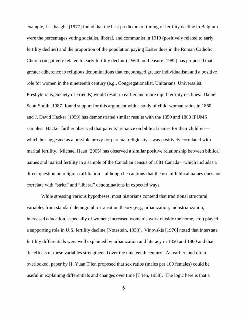
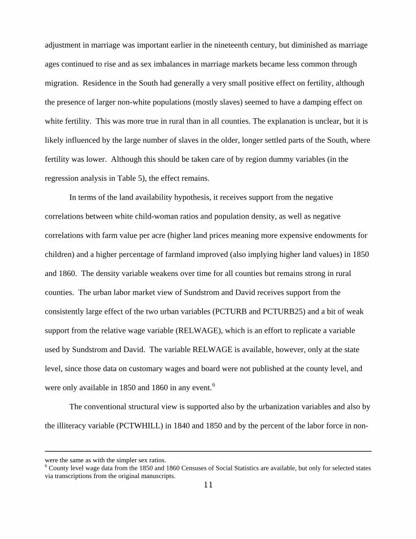
transition only commenced from about the 1870s [Haines, 2000]. Table 2 provides a view of child-

woman ratios estimated from census data (children aged 0-4 years per 1,000 women aged 20-44

years) by race, rural-urban residence, and region for the period 1800 to 1860. These data are also

depicted in Figures 1 and 2. While it is clear that these ratios suffer from shortcomings as measures

of fertility, namely that they are net of child and adult female mortality and that they also reflect

relative underenumeration of young children and adult women, they are the best we have for the

early nineteenth century. A comprehensive Birth Registration Area (consisting of ten states and the

District of Columbia) was not formed until 1915, and it did not cover the whole United States until

3 At the present time, published census age structures which allow the calculation of child-woman ratios at the county level exist only for 1800 to 1860, and then for 1930 to 1990. There exists now, however, a 100% sample of the 1880 Census of the United States which will allow special tabulations for that date and a similar analysis.

9

1933. We are forced to rely on census-based measures, even for the national estimates made by

own-children methods [Haines, 1989; Hacker, 2003]. Further, it is not clear what portion of the

decline in child-woman ratios between 1800 and 1860 originated in changes in marital fertility, in

rising mortality, or in the rising age at marriage and proportions married [Haines, 1996]. New

evidence on antebellum adult life expectancies [Pope, 1992] suggests that a significant portion of

the national decline in child-woman ratios before 1860 was probably due to changes in mortality

[Hacker, 2003]. Large regional differentials in child-woman ratios suggest that marital fertility

decline probably began in some parts of the nation (New England and the Mid-Atlantic) earlier,

however, and evidence from community-based studies and genealogies supports this inference

[Smith, 1973; Wells, 1971; Main, 2006]. But the early nineteenth century census data do not

permit these causes to be disentangled. Only the micro data from the IPUMS (Integrated Public

Use Microdata Series) permit this, and they do not begin until 1850.

Several major conclusions arise from looking at Table 2 and Figures 1 and 2. First, there

was a fairly consistent overall decline in child-woman ratios from 1810 onwards, and the decline

was consistent from 1800 onwards in most of the regions (see Figure 1). Second, there was a

decline in both rural and urban areas (see Figure 2). This, of course, casts some doubt on the

comprehensiveness of the land availability hypothesis. Third, there were substantial differences

across regions. As expected, the oldest settled regions (New England, Middle Atlantic, and South

Atlantic) had child-woman ratios which were the lowest, while areas further west, the East North

and South Central regions, had considerably higher fertility ratios. But they too decline with time.

Compositional effects (i.e., the mix of frontier and longer settle populations, and rural and urban

populations) clearly influenced this, but convergence was taking place.

10

A list of the variables to be used in the analysis is provided in Table 3. All variables were

drawn from the Censuses of Population, Agriculture, and Manufacturing. The earliest censuses

lacked economic data. Only in 1820 is there some information about the distribution of occupations

by sector (broken down only by agriculture, commerce, and manufacturing). In 1840, a greater

abundance of economic and social data becomes available. It should be noted that the child-

woman ratio we use is children aged 0-9 years per 1,000 women aged 16-44 years for the censuses

of 1800 to 1820, and children aged 0-9 years per 1,000 women aged 15-49 years for the censuses of

1830 to 1860. No effort was made to interpolate the age structures, which varied across the

censuses. In neither case are they the same as those given in Table 2, which were estimated by

Grabill, Kiser, and Whelpton [1958] and the U.S. Bureau of the Census [1975].

The distribution of variables may be seen in Table 4, which presents the zero order

correlations between the county child-woman ratios and the various explanatory variables. For all

the censuses, the white sex ratio, urbanization, density, the percent of the county population which

was nonwhite, and the location (region or whether in the South) are available. The other variables,

as mentioned, are present only in the later censuses. The table has two panels, one for all counties

and one for rural counties only. The latter are defined as having no population in an incorporated

place of 2,500 and over.4 As shown in the table, density and urbanization are consistently

negatively correlated with child-woman ratios. This supports several of the hypotheses (land

availability, urban labor markets, the conventional structural explanation), but may also reflect

differentials in infant and child mortality. The sex ratio had a large and positive effect on fertility

ratios early on, but the effect weakened over time.5 This is quite consistent with a view that

4 It is the case that some of these counties had population in minor civil divisions of smaller size that might be considered “urban.” It was decided to use the official census definition. 5 Experiments were done with more refined sex ratios, e.g., males per 100 females in the childbearing years. The results

11

adjustment in marriage was important earlier in the nineteenth century, but diminished as marriage

ages continued to rise and as sex imbalances in marriage markets became less common through

migration. Residence in the South had generally a very small positive effect on fertility, although

the presence of larger non-white populations (mostly slaves) seemed to have a damping effect on

white fertility. This was more true in rural than in all counties. The explanation is unclear, but it is

likely influenced by the large number of slaves in the older, longer settled parts of the South, where

fertility was lower. Although this should be taken care of by region dummy variables (in the

regression analysis in Table 5), the effect remains.

In terms of the land availability hypothesis, it receives support from the negative

correlations between white child-woman ratios and population density, as well as negative

correlations with farm value per acre (higher land prices meaning more expensive endowments for

children) and a higher percentage of farmland improved (also implying higher land values) in 1850

and 1860. The density variable weakens over time for all counties but remains strong in rural

counties. The urban labor market view of Sundstrom and David receives support from the

consistently large effect of the two urban variables (PCTURB and PCTURB25) and a bit of weak

support from the relative wage variable (RELWAGE), which is an effort to replicate a variable

used by Sundstrom and David. The variable RELWAGE is available, however, only at the state

level, since those data on customary wages and board were not published at the county level, and

were only available in 1850 and 1860 in any event.6

The conventional structural view is supported also by the urbanization variables and also by

the illiteracy variable (PCTWHILL) in 1840 and 1850 and by the percent of the labor force in non-

were the same as with the simpler sex ratios. 6 County level wage data from the 1850 and 1860 Censuses of Social Statistics are available, but only for selected states via transcriptions from the original manuscripts.

12

agricultural activity (PCTNONAG) in 1820 and 1840. The signs were in the expected direction

and the correlations were modest. The variable for the estimated percent of the labor force in

manufacturing (PCTMFGLB) is consistent with the structural view, but the correlation is only

moderate in 1850. Wealth per free person (WEALTHPC) also has reasonable and expected

negative signs in 1850 and 1860, although the negative correlation in rural counties could suggest a

problem with the land availability/target bequest hypothesis. The variable for transport

connections (TRANSPOR) for 1840-1860 is reasonably large and negative, reflecting a

modernization of the local area–bringing it to closer contact with outside markets and society in

general. The influence of a higher proportion of foreign-born population in the county (for 1850

and 1860) had a significant negative effect in 1850 but no effect in 1860.

Finally, the ideational hypothesis about fertility transition and differentials does get some

validation from the variable PRELNEW, which is the proportion of total church accommodations

which were Congregationalist, Society of Friends (Quaker), Presbyterian, Unitarian, and

Universalist. We must make do with data on churches, since the U.S. Census has never asked a

question of individuals on religion because of issues of separation of church and state. In any

event, counties with a greater proportion of these religious groups (albeit imperfectly measured)

also had lower fertility. If this proxy does, in some way, gauge the spread of individualism and

greater willingness to assume control of one’s own life decisions, then there is room to support this

particular approach to the issues of differential fertility and fertility decline.

In terms of regional results, there are no surprises. The older areas, the New England,

South Atlantic, and Middle Atlantic regions had a negative relationship to child-woman ratios,

while western areas, the Midwest (East and West North central regions) and the western South

(East and West South Central regions) generally had a positive relationship. This is in accord with

13

the general west to east gradient in fertility ratios. Being in the South had a weak positive

relationship for all counties, but an ambiguous one for rural counties. Those coefficients were

statistically insignificant, in any event. Higher rural white Southern fertility did not appear to be as

large an effect before the Civil War as it was later [U.S. Bureau of the Census, 1975, Series B 67-

98].

These variables were placed in a set of straightforward OLS multivariate regressions to

account for differences in child-woman ratios across counties from 1800 to 1860. These results are

reported in Table 5. The regressions do well in explaining the variation in fertility ratios across

counties, accounting for more than 50 percent of variation in all but one case (rural counties in

1860). The results observed in the correlations are generally confirmed with some interesting

differences. Urbanization was consistently and negatively related to fertility ratios. When density

was in the same equation (first panel of Table 5), density was not significant. It was if the

urbanization variable was omitted from the equation. In the equations for rural counties, the density

coefficient remained negative and significant throughout. These results tend to give greater support

to the labor market view of Sundstrom and David rather than the land availability hypothesis

(although lower child-woman ratios in urban areas may also reflect higher infant and child

mortality and lower nuptiality). They also support the Carter, Ransom and Sutch hypothesis of the

growing importance of life cycle saving. Other variables in the regressions, however, provide some

support for the land availability view. Average farm values per acre and the percent of farmland

which was improved both had negative and significant coefficients in 1850 and 1860 for all

counties, consistent with higher land values and more settled agriculture creating incentives to

reduce family size. In 1850, however, the coefficient on value per acre was positive in rural

counties, and the same coefficient was statistically insignificant in 1860. These results run counter

14

to the findings of poor performance of the land availability hypothesis by Carter, Ransom and

Sutch in their study. On the other hand, the labor market hypothesis, as well as the conventional

structural view, receive some backing from the negative and significant coefficients on the percent

of the labor force in nonagricultural activities (1820 and 1840) and the strong effect of the

transportation variable (1840, 1850, and 1860). The positive and significant coefficients on adult

white illiteracy (1840 and 1850) are also supportive of the structuralist perspective. The relative

wage variable provides no confirmation of the labor force theory, and indeed is even positive (the

opposite to expected sign) and significant in 1860. It is, however, a state-level variable.

The sex ratio, a proxy for the marriage market, showed the expected positive and significant

effects early in the nineteenth century, but that effect gradually diminished and even became

negative by 1840. Thus there is support for the view that adjustments in nuptiality played an

important role in the fertility transition at least in the early stages, a more purely demographic

perspective on the issue.

The ideational hypothesis also finds some confirmation. The religion variable

(PRELGNEW) remains negative and significant in the multivariate framework. Counties with a

higher proportion of the increasingly liberal and individualistic denominations were more likely to

have lower fertility, holding region and economic and demographic structure constant. Finally, the

level of wealth per free person seemed to have little impact on fertility ratios. But the percent of

foreign born by county did have a negative and significant relation to fertility ratios, even holding

urbanization constant. This is puzzling, given the finding that the foreign born often had higher

birth rates [Spengler, 1930], but the early stages of the mass migrations from Europe in the 1840s

and 1850s undoubtedly had some disruptive effects.

15

Tables 4 and 5 also presents two variables, WCURRMAR and WLABFORC, using data

aggregated from the 1850 and 1860 IPUMS samples [Ruggles and Sobek, 1997]. These individual-

level, one-percent samples of the original manuscript census records allow us to estimate women’s

current marital status and labor force participation at the county level or higher level of

aggregation. For each county, we calculated the percentage of women age 20-49 who were

imputed as having a spouse present in the household [see Ruggles, 1995 for details of the

imputation procedure]. We repeated the aggregation procedure for each state economic area

(SEA)—an aggregation of contiguous counties identified by the 1950 census sharing similar

economic characteristics—and state. If there were enough women in the county age 20-49 to

obtain a reasonably accurate estimate (using an arbitrary cut-off of at least 30 cases), we attached

the estimate to the county-level dataset. If there were not enough cases, we relied on the SEA- or

state-level estimates.7 We also constructed a variable on women’s economic opportunity by

aggregating the percentage of single women age 20-49 currently in the paid labor force. The

“independence” and “gains to marriage” theories contend that men and women will increasingly

postpone marriage or disrupt current marriages as educational attainment and job opportunities for

women improve. The relative lack of economic opportunity for young southern white women

outside the home, for example, may have increased the cultural incentive for marriage in the

antebellum South and helped to boost the region’s fertility [Hacker, 2006].

Women’s nuptiality (WCURRMAR) was included in 1850 and 1860. The variable was

consistently significant and the effect was large. It modestly improved the performance of the

models; the adjusted r-square for all counties in 1850, for example, increased from 0.561 to 0.575.

7 Of the 1,589 counties in 1850, the percentage of women currently married (WCURRMAR) was aggregated at the county level in 665 counties (42%), at the SEA level in 815 counties (50%), and at the state level in 357 counties (9%). Of the 1,974 counties in 1860, WCURRMAR was calculated at the county level for 918 counties (44%), SEA level for

16

Its inclusion, however, resulted in only modest change to the coefficients of the existing variables.

None of the coefficients changed sign and all but one of the coefficients significant at the .05 level

in the earlier models remained significant with the addition of women’s nuptiality. The one

exception was the white sex ratio in the 1860 models, whose coefficient only remained significant

at the 10% level when women’s nuptiality was included, suggesting that the sex ratio was a

reasonable proxy of marriage in the 1800-1840 models. Finally, women’s economic opportunity,

while having the expected negative sign, did not prove to be statistically significant.

DATA FOR THE INDIVIDUAL-LEVEL ANALYSIS

The data set used in the second part of the analysis is individual-level data in the 1850 and

1860 IPUMS samples [Ruggles and Sobek, 1997]. These samples, constructed at the University of

Minnesota Population Center, were drawn from the original manuscript records of the census of the

free population. Although neither census included questions on relationship to household head,

marital status, or fertility, census marshals were instructed to record individuals in a specified order

beginning with the head of household and followed by the spouse, children in order of age,

relatives and non-relatives. When combined with surname, age, and sex, it is possible to impute

the relationship of each individual to the household head and the position of each individual’s

spouse and children with a high degree of confidence. When tested against the 1880 IPUMS

sample—the first census to record each individual’s relationship to the household head—the

imputation procedure correctly identified over 99% of spouses and 97% of children.

The imputed relationship and own children variables in 1850 and 1860 IPUMS samples

allow us to attach directly model marital fertility (here defined as the number of own children under

937 counties (44%), and at the state level for 251 counties (12%).

17

age 5 in the household). There are several advantages to this approach. Most importantly, it allows

us to test hypotheses of U.S. fertility decline that emphasizes the importance to fertility decline

within marriage. Moreover, measurement of some variables at the individual level—literacy and

real estate wealth, for example—can reduce the possibility of spurious correlations inherent with

ecological regression. Finally, we can include likely correlates of martial fertility, such as age,

nativity, and spouse’s occupation in the model.

Despite these advantages, there remain a few limitations to the IPUMS samples. Although

manuscript records of the Census of Agriculture are available for some states and counties,

individuals in the IPUMS samples have not been linked to their farm holdings. Thus, we are forced

to link the individual-level data to the county-level dataset used in the first part of this analysis and

treat the data as contextual variables. We also lack information on the duration of each woman’s

current marriage. As a result, a model of own children under age 5 will include many women who

were married for only a portion of the five years preceding the census and identify correlates of

nuptiality and marital fertility. To reduce this source of bias, we further restrict the sample to

currently married women with at least one surviving child over age 5 in the household.8 Thus, only

fecund women are included. Finally, like child-woman ratios, the number of own children under

age 5 in the household is net of mortality. Unavoidably, our model of marital fertility will include

some unknown influence of differential mortality.

AN ANALYSIS OF THE ANTEBELLUM FERTILITY TRANSITION IN THE UNITED

STATES USING THE 1850 AND 1860 IPUMS SAMPLES

8 Because our data do not allow us to identify stepchildren, it is still likely that come women in the model universe were not married the entire five-year period preceding the census.

18

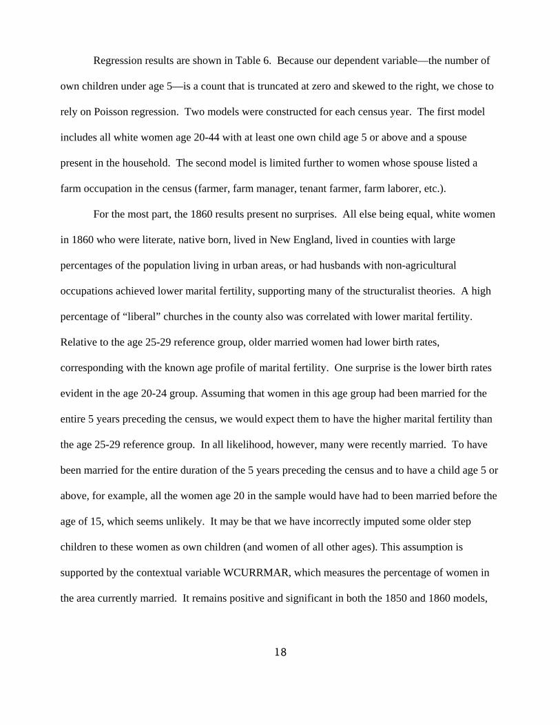
Regression results are shown in Table 6. Because our dependent variable—the number of

own children under age 5—is a count that is truncated at zero and skewed to the right, we chose to

rely on Poisson regression. Two models were constructed for each census year. The first model

includes all white women age 20-44 with at least one own child age 5 or above and a spouse

present in the household. The second model is limited further to women whose spouse listed a

farm occupation in the census (farmer, farm manager, tenant farmer, farm laborer, etc.).

For the most part, the 1860 results present no surprises. All else being equal, white women

in 1860 who were literate, native born, lived in New England, lived in counties with large

percentages of the population living in urban areas, or had husbands with non-agricultural

occupations achieved lower marital fertility, supporting many of the structuralist theories. A high

percentage of “liberal” churches in the county also was correlated with lower marital fertility.

Relative to the age 25-29 reference group, older married women had lower birth rates,

corresponding with the known age profile of marital fertility. One surprise is the lower birth rates

evident in the age 20-24 group. Assuming that women in this age group had been married for the

entire 5 years preceding the census, we would expect them to have the higher marital fertility than

the age 25-29 reference group. In all likelihood, however, many were recently married. To have

been married for the entire duration of the 5 years preceding the census and to have a child age 5 or

above, for example, all the women age 20 in the sample would have had to been married before the

age of 15, which seems unlikely. It may be that we have incorrectly imputed some older step

children to these women as own children (and women of all other ages). This assumption is

supported by the contextual variable WCURRMAR, which measures the percentage of women in

the area currently married. It remains positive and significant in both the 1850 and 1860 models,

19

suggesting the strong possibility that we are including some recently married women in the model

universe.

In 1860, nativity proved to be a significant at both the individual and county levels. The

marital fertility of foreign born women, all else being equal, was over 20% higher than native born

women. Interestingly, the percentage of the population in a county that was foreign born was

negatively correlated with marital fertility. It is unclear what mechanisms were at work; modern

researchers have not followed the lead of nineteenth-century nativist observers such as Francis A.

Walker who blamed immigrants for falling native born fertility. Still the relationship holds. The

percentage of the population that was non-white also was negatively correlated with white marital

fertility in 1860.

There is mixed support for the various economic theories. Although the sign is in the

expected direction, the availability of transportation (TRANSPOR) is not significant in the

individual-level regressions. Although women living in counties with large urban populations had

lower marital fertility in both census years, the relative wage variable RELWAGE provides

contradictory evidence of the labor force theory. Contrary to expectations, it has a positive sign

and is statistically significant in 1860. It is, however, negatively correlated with marital fertility in

1850. The individual-level regressions also provide mixed support for the land availability and

target-bequest hypotheses. Although average farm values per acre remains insignificant in both

census years, the percentage of farmland improved was negatively correlated with marital fertility

in 1850 and had a negative sign in 1860. More impressive, despite the negative correlations

between per capita wealth and child-woman ratios at the county level, couples’ real estate wealth

(natural logged) was positively correlated with marital fertility in both 1850 and 1860. Taken

together, these variables suggest that couples with limited real estate holdings to bequest or who

20

lived in areas with limited farmland to purchase as endowments for children were more likely to

limit their number of births. Another interpretation is possible, however. Since socio-economic

status and wealth have been shown to be negatively correlated with mortality in the mid nineteenth-

century United States [Ferrie 2003], it may be that children of couples with greater real estate

wealth simply experienced lower rates of infant mortality.

A few results for the 1850 census do not correspond with the 1860 results. While having

the expected positive sign, foreign birth was not significantly correlated with marital fertility in

1850. The percentage of church accommodations with a positive role for women, while having the

expected negative sign, also was not significantly correlated with marital fertility. Regional

differentials in marital fertility are not nearly as pronounced as they were in 1860 and, in the case

of some of the most recently settled regions, were not significantly different from that of the

reference group of New England. And as mentioned earlier, the relative wage variable returned

different results.

There are several possible explanations for the inconsistent results. First, differential

mortality likely played a greater role in 1850 than it did in 1860. The year preceding the 1850

census corresponded with an epidemic of cholera, which hit infants and urban areas especially hard

[Rosenberg 1962; Vinovskis, 1978]. Second, it is likely that true marital fertility differentials were

less pronounced in 1850 than in 1860. Evidence of parity-dependent fertility control in the United

States is only first detectable in the years preceding the 1860 census, and then only in the Northeast

[Hacker, 2003]. Evidence of parity-dependent control in other regions comes much later. Although

there is some evidence that New England couples were effectively “spacing” their children before

1850 [Main 2006], it is nonetheless probable that majority of the population did not practice

21

conscious marital fertility control and that the small differentials in marital fertility that did exist in

1850 are difficult to detect amidst larger differentials in marriage and mortality.

CONCLUDING COMMENTS

This paper is a first pass at a new analysis of the early fertility transition for the white

population of the United States in the nineteenth century. It uses aggregate county-level data, some

of which have not been much exploited for this purpose, and the recently constructed 1850 and

1860 IPUMS samples. New variables have been created from other data sources to supplement the

county-level data, namely the urban populations of the counties from 1790 onwards as well as

county areas, which allow calculations of density. More will need to be done, including analysis of

changes over decades and fixed effects models.

While analysis of change over time using a time series of cross sections is not perfect, some

useful results have appeared. The major competing hypotheses concerning the early American

fertility transition are: the land availability hypothesis, the local labor market/child default

hypothesis, the conventional structuralist view, and the ideational hypothesis. All receive some

support from the data here. Using the county-level dataset, we noted that support for the land

availability view is weakened by the finding that, when population density and percent urban are

both in the regression models, urbanization dominates. This lends more credence to the local labor

market/child default hypothesis. But structural variables (illiteracy, urbanization, transport) also

demonstrate some power in explaining cross sectional variation. The ideational view also finds

support, using a variable on religion in 1850 and 1860. But these different perspectives are not

necessarily mutually exclusive. More likely, a number of processes were underway, all of which

contributed to the unusual early fertility transition in the United States.

22

Many theories of U.S. fertility decline emphasize the importance of fertility decline within

marriage. Although many of the proposed mechanisms may act as simple Malthusian adjustments

to marriage—decreased land availability, for example, may reduce fertility by reducing nuptiality

rather than causing couples to engage in conscious fertility control—our individual-level models of

marital fertility suggest that the emphasis on neo-Malthusian adjustments in not entirely misplaced.

In particular, we note that the individual-level data, in addition to providing support for traditional

structural explanations, provide support for land availability/target-bequest theories. We caution,

however, that differential mortality may still bias the results. Counter-intuitively, we may need to

focus on nineteenth-century mortality differentials to learn more about U.S. fertility decline.

23

REFERENCES

Bateman, Fred and James D. Foust. 1974. “A Sample of Rural Households Selected from the 1860

Manuscript Censuses.” Agricultural History. Vol. 48, No. 1 (January). pp. 75-93.

Carter, Susan M., Roger L. Ransom, and Richard Sutch. 2004. “Family Matters: The Life-Cycle

Transition and the Antebellum American Fertility Decline.” In Timothy W. Guinnane,

William Sundstrom, and Warren Whatley, eds. History Matters: Essays on Economic

Growth, Technology, and Demographic Change. Stanford, CA: Stanford University Press.

pp. 271-327.

Coale, Ansley J., and Norfleet W. Rives, Jr. 1973. “A Statistical Reconstruction of the Black

Population of the United States, 1880-1970: Estimates of True Numbers by Age and Sex.”

Population Index. Vol. 39, No. 1 (January). pp. 3-36.

Coale, Ansley J., and Susan Cotts Watkins, eds. 1986. The Decline of Fertility in Europe.

Princeton, NJ: Princeton University Press.

Coale, Ansley J., and Melvin Zelnik. 1963. New Estimates of Fertility and Population in the United

States: A Study of Annual White Births from 1855 to 1960 and of Completeness of

Enumeration in the Censuses from 1880 to 1960. Princeton, NJ: Princeton University Press.

Earle, Carville, Changyong Cao, John Heppen, and Samuel Otterstrom. 1999. The Historical

United States County Boundary Files 1790 - 1999 on CD-ROM. Geoscience Publications.

Louisiana State University.

Easterlin, Richard A. 1976. “Population Change and Farm Settlement in the Northern United

States.” Journal of Economic History. Vol. 36, No. 1 (March). pp. 45-75.

Easterlin, Richard A., George Alter, and Gretchen Condran. 1978. “Farms and Farm Families in

Old and New Areas: The Northern States in 1860.” In Tamara K. Hareven and Maris A.

Vinovskis, eds. Family and Population in Nineteenth-Century America. Princeton, NJ:

Princeton University Press. pp. 22-84.

Ferrie, Joseph P. 2003. “The Rich and the Dead: Socioeconomic Status and Mortality in the United

States, 1850-1860.” In Costa, Dora L. (ed.), Health and Labor Force Participation Over the

Life Cycle: Evidence from the Past (Chicago: University of Chicago Press) pp. 11-50.

Forster, Colin, and G.S.L. Tucker. 1972. Economic Opportunity and Whiter American Fertility

Ratios, 1800-1860. New Haven: Yale University Press.

24

Grabill, Wilson H., Clyde V. Kiser, and Pascal K. Whelpton. 1958. The Fertility of American

Women. NY: Wiley.

Haan, Michael. 2005. “Studying the Impact of Religion on Fertility in Nineteenth-Century Canada:

The Use of Direct Measures and Proxy Variables.” Social Science History. Vol. 29, No. 3

(Fall). pp. 373-411.

Hacker, J. David. 1999. “Child Naming, Religion, and the Decline of Marital Fertility in

Nineteenth-Century America.” The History of the Family: An International Quarterly 43:

339-65.

Hacker, J. David. 2003. “Rethinking the ‘Early’ Decline of Marital Fertility in the United States,”

Demography. Vol. 4, No. 4 (November). pp. 605-620.

Hacker, J. David. 2006. “Economic, Demographic, and Anthropometric Correlates of First

Marriage in the Mid Nineteenth-Century United States,” Center for Population Economics

Working Paper Series. University of Chicago.

Haines, Michael R. 1989. “American Fertility in Transition: New Estimates of Birth Rates in the

United States, 1900-1910.” Demography. Vol. 26, No. 1 (February). pp. 137-148.

Haines, Michael R. 1996. “Long Term Marriage Patterns in the United States from Colonial Times

to the Present.” The History of the Family: An International Quarterly. Vol. 1, No. 1. pp.

15-39.

Haines, Michael R. 1998. “Estimated Life Tables for the United States, 1850-1910.” Historical

Methods. Vol. 31, No. 4 (Fall). pp. 149-169.

Haines, Michael R. 2000. “The Population of the United States, 1790-1920.” In Stanley Engerman

and Robert Gallman, eds. The Cambridge Economic History of the United States. Vol. II:

The Long Nineteenth Century. NY: Cambridge University Press. pp. 143-205.

Knodel, John, and Etienne van de Walle. 1979. “Lessons from the Past: Policy Implications of

Historical Fertility Studies.” Population and Development Review. Vol. 5, No. 2 (June). pp.

217-245.

Leet, Donald R. 1976. “The Determinants of Fertility Transition in Antebellum Ohio.” Journal of

Economic History. Vol. 36, No. 2 (June). pp. 359-378.

Leasure, W. J. (1982). “La baisse de la fécondité aux Etat-Unis de 1800 a 1860.” Population 37(3):

607-622.

25

Lesthaeghe, Ron J. 1977. The Decline of Belgian Fertility, 1800-1970. Princeton, New Jersey:

Princeton University Press.

Lesthaeghe, Ron. 1980. “On the Social Control of Human Reproduction.” Population and

Development Review. Vol. 6, No. 4 (March). pp. 527-548.

Lesthaeghe, Ron. 1983. “A Century of Demographic and Cultural Change in Western Europe: An

Exploration of Underlying Dimensions.” Population and Development Review. Vol. 9, No.

3 (September). pp. 411-435.

Long, John H. 2001. “Building Longevity into the Design of a Historical Geographic Information

System: The Atlas of Historical County Boundaries.” Paper presented at the annual

meetings of the Social Science History Association. Chicago. (November).

McInnis, R. M. 1977. “Childbearing and Land Availability: Some Evidence from Individual

Household Data.” In Ronald Demas Lee, ed. Population Patterns in the Past. New York:

Academic Press. pp. 201-227.

Main, G. L. 2006. “Rocking the Cradle: Downsizing the New England Family,” Journal of

Interdisciplinary History. Vol. 37, No. 1 (Summer), pp. 35-58.

Notestein, Frank W. 1953. “The Economics of Population and Food Supplies. I. The Economic

Problems of Population Change.” Proceedings of the Eighth International Conference of

Agricultural Economists. London, England: Oxford University Press.

Preston, Samuel H., and Michael R. Haines. 1991. Fatal Years: Child Mortality in Late Nineteenth

Century America. Princeton, NJ: Princeton University Press.

Rosenberg, Charles E. 1962. The Cholera Years: The United States in 1832, 1849, and 1866

(Chicago: Univ. of Chicago Press)

Ruggles, Steven. 1995. “Family Interrelationships.” Historical Methods 28: 52-58.

Ruggles, S., M. Sobek et al. 1997. Integrated Public Use Microdata Series: Version 2.0.

Minneapolis: Historical Census Projects, University of Minnesota. Available on-line at

http://www.ipums.org.

Ruggles, Steven. 2003. “Multigenerational Families in Nineteenth-Century America.” Continuity

and Change. Vol. 18, Part 1 (May). pp. 139-165.

26

Schapiro, Morton Owen. 1986. Filling Up America: An Economic-Demographic Model of

Population Growth and Distribution in the Nineteenth-Century United States. Greenwich,

CT: JAI Press.

Smith, Daniel Scott. 1973. “Population, Family and Society in Hingham, Massachusetts, 1635-

1880.” Ph.D. thesis. Department of History, University of California, Berkeley.

Smith, Daniel Scott. 1977. “A Homeostatic Demographic Regime: Patterns in West European

Family Reconstitution Studies.” In Ronald D. Lee, ed. Population Patterns in the Past. New

York: Academic Press. pp. 19-51.

Smith, Daniel Scott. 1987. “‘Early’ Fertility Decline in America: A Problem in Family History.”

Journal of Family History. Vol. 12, Nos. 1-3. pp. 73-84.

Spengler, J.J. 1930. “The Fecundity of Native and Foreign-Born Women in New England.”

Brookings Institution Pamphlet Series. No. II (1).

Steckel, Richard H. 1986. “A Dreadful Childhood: Excess Mortality of American Slaves.” Social

Science History. Vol. 10, No. 4 (Winter). pp. 427-465.

Sundstrom, William A., and Paul A. David. 1988. “Old-Age Security Motives, Labor Markets, and

Farm Family Fertility in Antebellum America.” Explorations in Economic History. Vol. 25,

No. 2 (April). pp. 164-197.

Thompson, Warren S., and P. K. Whelpton. 1933. Population Trends in the United States. New

York. McGraw-Hill.

T’ien, H. Yuan. 1959. “A Demographic Aspect of Interstate Variations in American Fertility, 1800-

1860.” The Milbank Memorial Fund Quarterly. Vol. 37. pp. 49-59.

U.S. Bureau of the Census. 1975. Historical Statistics of the United States from Colonial Times to

1970. Wash., DC: G.P.O.

U.S. Bureau of the Census. 1985. Statistical Abstract of the United States, 1986. Wash., DC:

G.P.O.

U.S. Bureau of the Census. 1997. Statistical Abstract of the United States, 1997. Wash., DC:

G.P.O.

U.S. Bureau of the Census. 2001. Statistical Abstract of the United States, 2001. Wash., DC:

G.P.O.

27

Vinovskis, Maris. 1976. “Socioeconomic Determinants of Interstate Fertility Differentials in the

United States in 1850 and 1860.” The Journal of Interdisciplinary History. Vol. 6, No. 3

(Winter). pp. 375-396.

Vinovskis, M. A. 1978. “The Jacobson Life Table of 1850: A Critical Re-examination from a

Massachusetts Perspective.” Journal of Interdisciplinary History 84: 703-24.

Wells, R. V. 1971. “Family Size and Fertility Control in Eighteenth-Century America: A Study of

Quaker Families.” Population Studies 46: 85-102.

Yasuba, Yasukichi. 1962. Birth Rates of the White Population of the United States, 1800-1860: An

Economic Analysis. Baltimore: The Johns Hopkins University Press.

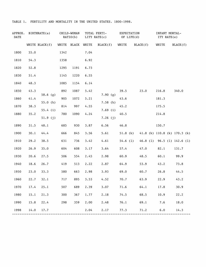
TABLE 1. FERTILITY AND MORTALITY IN THE UNITED STATES. 1800-1998. APPROX. BIRTHRATE(a) CHILD-WOMAN TOTAL FERTI- EXPECTATION INFANT MORTAL- DATE RATIO(b) LITY RATE(c) OF LIFE(d) ITY RATE(e) WHITE BLACK(f) WHITE BLACK WHITE BLACK(f) WHITE BLACK(f) WHITE BLACK(f) 1800 55.0 1342 7.04 1810 54.3 1358 6.92 1820 52.8 1295 1191 6.73 1830 51.4 1145 1220 6.55 1840 48.3 1085 1154 6.14 1850 43.3 892 1087 5.42 39.5 23.0 216.8 340.0 58.6 (g) 7.90 (g) 1860 41.4 905 1072 5.21 43.6 181.3 55.0 (h) 7.58 (h) 1870 38.3 814 997 4.55 45.2 175.5 55.4 (i) 7.69 (i) 1880 35.2 780 1090 4.24 40.5 214.8 51.9 (j) 7.26 (j) 1890 31.5 48.1 685 930 3.87 6.56 46.8 150.7 1900 30.1 44.4 666 845 3.56 5.61 51.8 (k) 41.8 (k) 110.8 (k) 170.3 (k) 1910 29.2 38.5 631 736 3.42 4.61 54.6 (l) 46.8 (l) 96.5 (l) 142.6 (l) 1920 26.9 35.0 604 608 3.17 3.64 57.4 47.0 82.1 131.7 1930 20.6 27.5 506 554 2.45 2.98 60.9 48.5 60.1 99.9 1940 18.6 26.7 419 513 2.22 2.87 64.9 53.9 43.2 73.8 1950 23.0 33.3 580 663 2.98 3.93 69.0 60.7 26.8 44.5 1960 22.7 32.1 717 895 3.53 4.52 70.7 63.9 22.9 43.2 1970 17.4 25.1 507 689 2.39 3.07 71.6 64.1 17.8 30.9 1980 15.1 21.3 300 367 1.77 2.18 74.5 68.5 10.9 22.2 1990 15.8 22.4 298 359 2.00 2.48 76.1 69.1 7.6 18.0 1998 14.0 17.7 2.04 2.17 77.3 71.2 6.0 14.3 --------------------------------------------------------------------------------------------------

TABLE 1 (cont.) (a) Births per 1000 population per annum. (b) Children aged 0-4 per 1000 women aged 20-44. Taken from U.S. Bureau of the Census [1975],

Series 67-68 for 1800-1970. For the black population 1820-1840, Thompson and Whelpton [1933], Table 74, adjusted upward 47% for relative under-enumeration of black children aged 0-4 for the censuses of 1820-1840.

(c) Total number of births per woman if she experienced the current period age-specific fertility rates throughout her life.

(d) Expectation of life at birth for both sexes combined. (e) Infant deaths per 1000 live births per annum. (f) Black and other population for CBR (1920-1970), TFR (1940-1990), e(0) (1950-1960), IMR (1920- (g) Average for 1850-59. (h) Average for 1860-69. (i) Average for 1870-79. (j) Average for 1880-84. (k) Approximately 1895. (l) Approximately 1904. Source: U.S. Bureau of the Census [1975, 1985, 1997, 2001]. Coale and Zelnik [1960]. Coale and Rives

[1973]. Haines [1998]. Preston and Haines [1991]. Steckel [1986].

TABLE 2. Number of Children Under 5 Years Old per 1,000 Women Aged 20-44 Years, by Race, Residence, and Region. United States, 1800-1860.

Year Region, Residence, Race 1800 1810 1820 1830 1840 1850 1860 United States, white population, adjusted 1342 1358 1295 1145 1085 892 905 United States, black population, adjusted ----- ----- ----- ----- ----- 1087 1072 United States, white population 1281 1290 1236 1134 1070 877 886 United States, urban white population 845 900 831 708 701 ----- ----- United States, rural white population 1319 1329 1276 1189 1134 ----- ----- New England, white population 1098 1052 930 812 752 621 622 New England, urban white population 827 845 764 614 592 ----- ----- New England, rural white population 1126 1079 952 851 800 ----- ----- Middle Atlantic, white population 1279 1289 1183 1036 940 763 767 Middle Atlantic, urban white population 852 924 842 722 711 ----- ----- Middle Atlantic, rural white population 1339 1344 1235 1100 1006 ----- ----- East North Central, white population 1840 1702 1608 1467 1270 1022 999 East North Central, urban white population ----- 1256 1059 910 841 ----- ----- East North Central, rural white population 1840 1706 1616 1484 1291 ----- ----- West North Central, white population ----- 1810 1685 1678 1445 1114 1105 West North Central, urban white population ----- ----- ----- 1181 705 ----- ----- West North Central, rural white population ----- 1810 1685 1703 1481 ----- ----- South Atlantic, white population 1345 1325 1280 1174 1140 937 918 South Atlantic, urban white population 861 936 881 767 770 ----- ----- South Atlantic, rural white population 1365 1347 1310 1209 1185 ----- ----- East South Central, white population 1799 1700 1631 1519 1408 1099 1039 East South Central, urban white population ----- 1348 1089 863 859 ----- ----- East South Central, rural white population 1799 1701 1635 1529 1424 ----- -----

Table 2 (cont.) Year Region, Residence, Race 1800 1810 1820 1830 1840 1850 1860 West South Central, white population ----- 1383 1418 1359 1297 1046 1084 West South Central, urban white population ----- 727 866 877 846 ----- ----- Mountain, white population ----- ----- ----- ----- ----- 886 1051 Mountain, urban white population ----- ----- ----- ----- ----- ----- ----- Mountain, rural white population ----- ----- ----- ----- ----- ----- ----- Pacific, white population ----- ----- ----- ----- ----- 901 1026 Pacific, urban white population ----- ----- ----- ----- ----- ----- ----- Pacific, rural white population ----- ----- ----- ----- ----- ----- ----- Source: U.S. Bureau of the Census [1975], Series B 67-98. (a) Adjusted data standardized for age of women, and allowance made for undercount in censuses; see text.

TABLE 3. Variable Names and Descriptions. VARIABLE DESCRIPTION WHCWRAT Child-woman ratio, white population: 1800-1820: children aged 0-9 years per 1,000 women aged 16-44 years. 1830-1860: children aged 0-9 years per 1,000 women aged 15-49 years. WHSEXRAT Sex ratio, white population: White males per 100 white females (all ages). DENSITY Population density: Persons per square mile. PCTURB Percent urban (in places 2,500 and over). PCTURB25 Percent of population in places 25,000 and over. PCTNW Percent of total population non-white. SOUTH =1 if the county was in the South, =0 otherwise. PCTNONAG Estimated percent of the labor force in non-agricultural activity. PCTWHILL Percent of white population aged 20 and over who were unable to read and write. PCTFOR Percent of the total population foreign born. PCTMFGLB Estimated percent of the white population aged 15-69 employed in manufacturing. PRELGNEW Percent of all church accommodations Congregationalist, Presbyterian, Unitarian, and Universalist. RELWAGE Ratio of estimated monthly wages of a common laborer with board to the monthly wages of a farmhand with board. (States only). TRANSPOR Variable=1 if the county was on a canal, river, or other navigable waterway in 1840. Otherwise=0. For 1850 and 1860, variable =1 if county on a railroad or navigable waterway. Otherwise=0. WEALTHPC 1850: Value of real estate per free person. 1860: Value of real and personal estate per free person. FARVALAC Average value of farm per acre (improved and unimproved). PCTACIMP Percent of farm acres improved. WCURRMARR Proportion of women aged 20-49 currently married. WLABFORCE Proportion of single women aged 20-49 in the labor force. Source: See text.

Table 4. Zero-Order Correlations with White Child-Woman Ratios. Counties, 1800-1860. YEAR: VARIABLE 1800 1810 1820 1830 1840 1850 1860 ALL COUNTIES WHSEXRAT 0.495 0.285 0.190 0.227 0.022 -0.160 0.126 DENSITY -0.202 -0.168 -0.164 -0.150 -0.122 -0.100 -0.080 PCTURB -0.288 -0.296 -0.320 -0.328 -0.381 -0.364 -0.363 PCTURB25 -0.147 -0.163 -0.169 -0.157 -0.169 -0.189 -0.182 PCTNW -0.426 -0.404 -0.288 -0.284 -0.100 -0.111 -0.169 SOUTH 0.097 0.015 0.066 0.005 0.172 0.109 0.065 TRANSPOR -0.363 -0.401 -0.410 PCTFOR -0.269 0.012 PCTNONAG -0.387 -0.499 PCTWHILL 0.382 0.245 PCTMFGLB -0.427 -0.290 WEALTHPC -0.261 -0.200 FARVALAC -0.178 -0.106 PCTACIMP -0.400 -0.487 PRELGNEW -0.283 -0.379 RELWAGE -0.222 -0.058 WCURRMAR 0.382 0.172 WLABFORC 0.146 REGIONS: New England -0.237 -0.312 -0.410 -0.398 -0.384 -0.348 -0.342 Middle Atlantic 0.027 -0.004 -0.140 -0.228 -0.310 -0.275 -0.277 East North Central 0.127 0.270 0.295 0.321 0.114 0.068 -0.059 West North Central 0.100 0.121 0.207 0.184 0.256 0.216 South Atlantic -0.268 -0.334 -0.272 -0.311 -0.193 -0.141 -0.144 East South Central 0.503 0.420 0.368 0.300 0.317 0.136 0.031 West South Central 0.053 0.060 0.108 0.181 0.201 0.260 Mountain -0.046 0.137 Pacific -0.058 0.153 N 417 571 753 982 1235 1611 2012

Table 4 (cont.) RURAL COUNTIES WHSEXRAT 0.496 0.284 0.171 0.200 -0.004 -0.187 0.102 DENSITY -0.559 -0.564 -0.556 -0.614 -0.526 -0.471 -0.495 PCTNW -0.495 -0.470 -0.349 -0.350 -0.152 -0.180 -0.261 SOUTH 0.029 -0.061 0.004 -0.064 0.126 0.042 -0.024 TRANSPOR -0.314 -0.344 -0.349 PCTFOR -0.205 0.120 PCTNONAG -0.264 -0.379 PCTWHILL 0.336 0.196 PCTMFGLB -0.288 -0.133 WEALTHPC -0.253 -0.230 FARVALAC -0.368 -0.404 PCTACIMP -0.326 -0.409 PRELGNEW -0.216 -0.286 RELWAGE -0.208 0.037 WCURRMAR 0.357 0.157 WLABFORC 0.216 REGIONS: New England -0.160 -0.239 -0.347 -0.321 -0.289 -0.239 -0.240 Middle Atlantic 0.035 0.015 -0.129 -0.221 -0.311 -0.262 -0.235 East North Central 0.123 0.267 0.284 0.310 0.075 0.050 -0.072 West North Central 0.099 0.118 0.213 0.180 0.248 0.190 South Atlantic -0.343 -0.413 -0.333 -0.375 -0.246 -0.194 -0.214 East South Central 0.505 0.424 0.359 0.290 0.310 0.110 -0.009 West South Central 0.067 0.059 0.102 0.180 0.192 0.252 Mountain -0.054 0.141 Pacific -0.075 0.153 N 396 540 709 919 1137 1434 1721

Table 5. Regression Results. White Child-Woman Ratios as the Dependent Variable. Counties. United States, 1800-1860. YEAR: ALL COUNTIES VARIABLE 1800 1810 1820 1830 1840 1850 1860 (coef) (signi (coef) (signi) (coef) (signi) (coef) (signi) (coef) (signi) (coef) (signi) (coef) (signi) CONSTANT 448.665 *** 1472.231 *** 1502.751 *** 1094.992 *** 1310.230 *** 1039.793 *** 491.895 *** WHSEXRAT 13.186 *** 2.243 *** 1.371 *** 0.979 ** -0.028 --- -0.204 *** -0.048 --- DENSITY -0.072 --- -0.018 --- 0.017 --- -0.009 --- 0.006 --- 0.041 --- 0.069 *** PCTURB -5.997 *** -6.219 *** -2.322 ** -5.748 *** -2.703 *** -2.354 *** -3.304 *** PCTNW -11.794 *** -10.433 *** -9.104 *** -7.890 *** -4.378 *** -2.799 *** -2.685 *** PCTNONAG -6.568 *** -4.283 *** TRANSPOR -84.107 *** -73.457 *** -42.938 *** PCTFOR -6.142 *** -0.354 --- PCTWHILL 2.788 *** 1.144 --- PCTMFGLB -0.456 --- 0.642 --- WEALTHPC -0.167 *** -0.005 --- FARVALAC -0.498 --- -0.449 ** PCTACIMP -2.213 *** -2.478 *** PRELGNEW -1.899 *** -2.245 *** RELWAGE 1469.313 --- 287.878 *** WCURRMAR 411.257 *** 498.504 *** WLABFORC 27.411 --- REGIONS: New England NI NI NI NI NI NI NI Middle Atlantic 171.475 *** 320.719 *** 358.403 *** 295.984 *** 215.754 *** 193.926 *** 173.863 *** East North Cent. 165.523 * 576.659 *** 606.578 *** 665.590 *** 416.531 *** 334.414 *** 325.132 *** West North Central 753.566 *** 767.102 *** 962.821 *** 592.177 *** 426.945 *** 379.783 *** South Atlantic 464.658 *** 547.060 *** 576.073 *** 621.370 *** 376.142 *** 246.043 *** 338.738 *** East South Cent. 727.827 *** 782.528 *** 779.338 *** 841.779 *** 588.406 *** 351.642 *** 406.174 *** West South Central 73.471 --- 791.707 *** 904.731 *** 704.285 *** 432.111 *** 502.085 *** Mountain 79.635 --- 694.100 *** Pacific 596.241 *** 662.734 *** Adj. R-squared 0.6542 0.6129 0.6134 0.6147 0.6160 0.5746 0.5649 F-ratio 99.39 *** 91.25 *** 109.48 *** 157.48 *** 153.29 *** 99.86 *** 119.68 *** N 417 571 753 982 1235 1611 2012

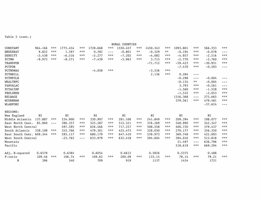
Table 5 (cont.)

RURAL COUNTIES CONSTANT 964.166 *** 1775.454 *** 1728.668 *** 1550.457 *** 1450.343 *** 1093.801 *** 566.353 *** WHSEXRAT 9.822 *** 1.597 *** 0.392 --- -0.801 ** -0.329 ** -0.194 *** -0.078 --- DENSITY -5.438 *** -6.516 *** -5.277 *** -7.202 *** -4.082 *** -4.957 *** -2.516 *** PCTNW -9.973 *** -8.271 *** -7.439 *** -5.963 *** 3.715 *** -2.770 *** -2.760 *** TRANSPOR -71.712 *** -59.423 *** -30.951 *** PCTFOR -7.470 *** -0.593 --- PCTNONAG -4.058 *** -3.536 *** PCTWHILL 2.136 *** 0.284 --- PCTMFGLB -0.298 --- -0.004 --- WEALTHPC -0.134 ** -0.004 --- FARVALAC 3.793 *** -0.261 --- PCTACIMP -1.560 *** -1.528 *** PRELGNEW -1.532 *** -2.053 *** RELWAGE 1316.368 --- 273.665 *** WCURRMAR 379.561 *** 479.481 *** WLABFORC -37.624 --- REGIONS: New England NI NI NI NI NI NI NI Middle Atlantic 137.887 *** 234.900 *** 330.997 *** 281.106 *** 241.849 *** 209.394 *** 198.077 *** East North Cent. 85.960 --- 396.357 *** 525.587 *** 515.321 *** 376.269 *** 348.990 *** 342.347 *** West North Central 497.595 *** 626.466 *** 717.227 *** 508.558 *** 400.720 *** 379.437 *** South Atlantic 338.108 *** 353.766 *** 479.301 *** 425.473 *** 328.030 *** 270.177 *** 356.350 *** East South Cent. 609.344 *** 595.117 *** 680.179 *** 647.410 *** 539.973 *** 369.748 *** 422.093 *** West South Central -23.765 --- 633.979 *** 632.418 *** 594.604 *** 394.016 *** 512.818 *** Mountain 21.497 --- 636.796 *** Pacific 518.619 *** 669.294 *** Adj, R-squared 0.6578 0.6384 0.6054 0.6612 0.5826 0.5375 0.488 F-ratio 109.46 *** 106.74 *** 109.62 *** 200.09 *** 133.15 *** 78.14 *** 79.21 *** N 396 540 709 919 1137 1434 1721

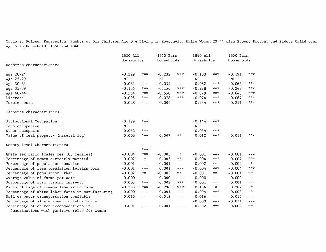
Table 6. Poisson Regression, Number of Own Children Age 0-4 Living in Household, White Women 20-44 with Spouse Present and Eldest Child over Age 5 in Household, 1850 and 1860 1850 All 1850 Farm 1860 All 1860 Farm Households Households Households Households Mother’s characteristics Age 20-24 -0.229 *** -0.232 *** -0.183 *** -0.191 *** Age 25-29 NI NI NI NI Age 30-34 -0.034 --- -0.034 --- -0.082 *** -0.065 *** Age 35-39 -0.156 *** -0.156 *** -0.278 *** -0.248 *** Age 40-44 -0.554 *** -0.550 *** -0.679 *** -0.640 *** Literate -0.095 *** -0.078 *** -0.074 *** -0.067 *** Foreign born 0.028 --- 0.004 --- 0.234 *** 0.211 *** Father’s characteristics Professional Occupation -0.189 *** -0.144 *** Farm occupation NI NI Other occupation -0.062 *** -0.064 *** Value of real property (natural log) 0.008 *** 0.007 ** 0.012 *** 0.011 *** County-level Characteristics *** White sex ratio (males per 100 females) -0.004 *** -0.003 * -0.001 --- -0.001 --- Percentage of women currently married 0.002 * 0.003 ** 0.004 *** 0.004 *** Percentage of population nonwhite -0.001 --- -0.001 --- -0.002 ** -0.002 * Percentage of free population foreign born -0.001 --- 0.001 --- -0.004 *** -0.004 *** Percentage of population urban -0.002 ** -0.002 ** -0.001 ** -0.001 ** Average value of farms per acre 0.000 --- 0.000 --- 0.000 --- 0.000 --- Percentage of farm acreage improved -0.003 *** -0.003 *** -0.001 --- -0.001 --- Ratio of wage of common laborer to farm -0.365 *** -0.296 *** 0.186 * 0.282 * Percentage of white labor force in manufacturing 0.000 --- -0.001 --- 0.004 *** 0.003 * Rail or water transportation available -0.019 --- -0.018 --- -0.016 --- -0.010 --- Percentage of single women in labor force -0.083 --- -0.071 --- Percentage of church accommodations in -0.001 --- -0.001 --- -0.002 *** -0.002 ** denominations with positive roles for women

Table 6 (cont.) Regions: New England NI NI NI NI Middle Atlantic 0.127 *** 0.081 * 0.118 *** 0.104 ** East North Central 0.138 *** 0.101 * 0.207 *** 0.207 *** West North Central 0.106 * 0.108 --- 0.197 *** 0.194 *** South Atlantic 0.219 *** 0.178 *** 0.262 *** 0.248 *** East South Central 0.199 *** 0.164 ** 0.286 *** 0.280 *** West South Central 0.125 * 0.061 --- 0.249 *** 0.248 *** Mountain -0.003 --- 0.039 --- 0.143 --- 0.144 --- Pacific 0.240 --- 0.084 --- 0.368 *** 0.400 *** Constant 1.185 *** 0.931 *** -0.142 --- -0.282 --- N 22,216 14,030 32,347 19,710 Adjusted R-squared 0.025 0.023 0.028 0.024 Log likelihood (28,146) (18,178) (41,169) (25,636) Source: 1850 and 1860 IPUMS samples (Ruggles and Sobek 1997) Notes: *** p<.001, ** p<.01, * p<.05, --- = not significant at least at a 10% level

1800 1810 1820 1830 1840

Year

600

700

800

900

1000

1100

1200

1300

1400

Chi

ld-W

om

an

Ratio

U .S.

Ur ban

Rur a l

Fig. 1. Chi ld-Woman Ratios.By Rural -Urban. U.S. 1800-1840.

1800 1810 1820 1830 1840 1850 1860

Year

500

1000

1500

2000

Ch

ild-W

om

an

Ra

tioU .S.

NE

MA

ENC

W NC

SA

ESC

W SC

Fig . 2. Child-Woman Ratios.By Region. U.S. 1800-1860.