NBER WORKING PAPER SERIES

OVER-REACTION IN MACROECONOMIC EXPECTATIONS

Pedro BordaloNicola Gennaioli

Yueran MaAndrei Shleifer

Working Paper 24932http://www.nber.org/papers/w24932

NATIONAL BUREAU OF ECONOMIC RESEARCH1050 Massachusetts Avenue

Cambridge, MA 02138August 2018

We thank Olivier Coibion, Xavier Gabaix, Yuriy Gorodnichenko, Luigi Guiso, Lars Hansen, David Laibson, Jesse Shapiro, Paolo Surico, participants at the 2018 AEA meeting, NBER Behavioral Finance Meeting, NBER Summer Institute, and seminar participants at EIEF, Ecole Politechnique, Harvard, and LBS for helpful comments. We acknowledge the financial support of the Behavioral Finance and Finance Stability Initiative at Harvard Business School and the Pershing Square Venture Fund for Research on the Foundations of Human Behavior. Gennaioli thanks the European Research Council for Financial Support under the ERC Consolidator Grant (GA 647782). We thank Johan Cassell, Francesca Miserocchi, Johnny Tang, and especially Spencer Kwon and Weijie Zhang for outstanding research assistance. The views expressed herein are those of the authors and do not necessarily reflect the views of the National Bureau of Economic Research.

NBER working papers are circulated for discussion and comment purposes. They have not been peer-reviewed or been subject to the review by the NBER Board of Directors that accompanies official NBER publications.

© 2018 by Pedro Bordalo, Nicola Gennaioli, Yueran Ma, and Andrei Shleifer. All rights reserved. Short sections of text, not to exceed two paragraphs, may be quoted without explicit permission provided that full credit, including © notice, is given to the source.

Over-reaction in Macroeconomic ExpectationsPedro Bordalo, Nicola Gennaioli, Yueran Ma, and Andrei ShleiferNBER Working Paper No. 24932August 2018JEL No. E03,E17,E32,E37

ABSTRACT

We study the rationality of individual and consensus professional forecasts of macroeconomic and financial variables using the methodology of Coibion and Gorodnichenko (2015), which examines predictability of forecast errors from forecast revisions. We report two key findings: forecasters typically over-react to their individual news, while consensus forecasts under-react to average forecaster news. To reconcile these findings, we combine the diagnostic expectations model of belief formation from Bordalo, Gennaioli, and Shleifer (2018) with Woodford’s (2003) noisy information model of belief dispersion. The forward looking nature of diagnostic expectations yields additional implications, which we also test and confirm. A structural estimation exercise indicates that our model captures important variation in the data, yielding a value for the belief distortion parameter similar to estimates obtained in other settings

Pedro BordaloSaïd Business SchoolUniversity of OxfordPark End StreetOxford, OX1 1HPUnited Kingdompedro.bordalo@sbs.ox.ac.uk

Nicola GennaioliDepartment of FinanceUniversità BocconiVia Roentgen 120136 Milan, Italynicola.gennaioli@unibocconi.it

Yueran MaThe University of ChicagoBooth School of Business5807 S. Woodlawn Ave.Chicago, IL 60637Yueran.Ma@chicagobooth.edu

Andrei ShleiferDepartment of Economics Harvard UniversityLittauer Center M-9 Cambridge, MA 02138and NBERashleifer@harvard.edu

2

I. Introduction

According to the Rational Expectations Hypothesis, market participants form their beliefs about

the future, and make decisions, on the basis of statistically optimal forecasts. A growing body of work tests

this hypothesis using survey data on the anticipations of households and professional forecasters. The

evidence points to systematic departures from statistical optimality, which take the form of predictable

forecast errors. Such departures have been documented in the cases of forecasting inflation and other macro

variables (Coibion and Gorodnichenko 2012, 2015, henceforth CG, Fuhrer 2017), the aggregate stock

market (Bacchetta, Mertens, and Wincoop 2009, Amromin and Sharpe 2013, Greenwood and Shleifer

2014, Adam, Marcet, and Buetel 2017), the cross section of stock returns (La Porta 1996, Bordalo,

Gennaioli, La Porta, and Shleifer 2017, henceforth BGLS), credit spreads (Greenwood and Hanson 2013,

Bordalo, Gennaioli, and Shleifer 2018), and corporate earnings (DeBondt and Thaler 1990, Ben-David,

Graham, and Harvey 2013, Gennaioli, Ma, and Shleifer 2016, Bouchaud, Kruger, Landier, and Thesmar

2017). Departures from optimal forecasts also obtain in controlled experiments (Hommes et al. 2004,

Beshears et al. 2013, Frydman and Nave 2016, Landier, Ma, and Thesmar 2017).

Various relaxations of the Rational Expectations Hypothesis have been proposed to account for the

data. In macroeconomics, the main approach builds on rational inattention and information rigidities (Sims

2003, Woodford 2003, Carroll 2003, Mankiw and Reis 2002, Gabaix 2014). This view maintains the

rationality of individual inferences, but relaxes the assumption of common information or full information

processing. This is often justified by arguing that acquiring or processing information entails significant

material and cognitive costs. To economize on these costs, agents revise their expectations sporadically, or

on the basis of selective news. As a consequence, expectations and decisions under-react to news relative

to the case of unlimited information capacity. In a novel empirical test of these theories, CG (2015) study

predictability of errors in consensus macroeconomic forecasts of inflation and other variables, and find

evidence consistent with under-reaction.

In finance, in contrast, although there is some evidence of momentum and under-reaction (Cutler,

Poterba, and Summers 1990, Jegadeesh and Titman 1993), the dominant puzzle is over-reaction to news.

This puzzle has been motivated by the evidence that stock prices move too much relative to the movements

3

in fundamentals both in the aggregate (Shiller 1981) and in the cross section (De Bondt and Thaler 1985).

The leading psychological mechanism for over-reaction is Tversky and Kahneman’s (1974) finding that,

in reacting to news, people tend to overweight “representative” events (Barberis, Shleifer and Vishny 1998,

Gennaioli and Shleifer 2010). For instance, exceptional past performance of a firm may cause

overweighting of the probability that this firm is “the next google” because googles are representative of

the group of well performing firms, even though they are objectively rare. This approach is not inconsistent

with limited information processing, but stresses that people infer too much from the information they

attend to, however limited, so that beliefs and decisions move too much with news (Augenblick and Rabin

2017, Augenblick and Lazarus 2017). BGLS (2017) look at the cross section of stock returns and analyst

expectations of earnings growth and find support for over-reaction driven by representativeness.

This state of research motivates two questions. First, which departure from rational expectations is

predominant, under- or over-reaction to news? Second, which mechanisms create these departures? Put

differently, can one account for the main features in the data using a parsimonious model capturing precise

cognitive mechanisms for under- and over-reaction?

This paper addresses these questions by studying the predictions of professional forecasters of 16

macroeconomic variables, which include and expand those considered by CG (2015). We use both the

Survey of Professional Forecasters (SPF) and the Blue Chip Survey, which gives us 20 expectations time

series in total (four variables appear in both surveys), including forecasts of real economic activity,

consumption, investment, unemployment, housing starts, government expenditures, as well as multiple

interest rates. We examine both consensus and individual level forecasts. SPF data are publicly available;

Blue Chip data were purchased and hand-coded for the earlier part of the sample.

Section 3 describes the patterns of over- and under-reaction in different series. We follow CG’s

methodology of measuring a forecaster’s reaction to news by their forecast revision, and of using this

forecast revision to predict the forecast error, computed as the difference between the realization and the

forecast. In this setting, under-reaction to news implies a positive correlation between forecast errors and

forecast revisions, while over-reaction to news implies the opposite. Unlike CG, we examine not only

4

consensus forecasts, defined as the average forecast across all analysts, but also individual ones. The

consequences of aggregating forecasts turn out to be crucial for understanding their properties.

For the case of consensus forecasts, we confirm the CG findings of under-reaction: the average

forecast revision positively predicts the average future forecast error for most series. At the individual level,

however, the opposite pattern emerges: for most series, the forecast revision of the average forecaster

negatively predicts the same forecaster’s future error. In stark contrast to the consensus results, at the level

of the individual forecaster over-reaction is the norm, under-reaction the exception. These results are

robust to several potential sources of predictability, including forecaster heterogeneity, small sample bias,

measurement error, nonstandard loss functions, and non-normality of shocks.

In Section 4 we propose a model that reconciles these seemingly contradictory findings. In our

setup, agents must predict the future value of a state that follows an AR(1) process. Each agent observes a

different noisy signal of the current value of this state. Forecaster-specific noise can capture either

inattention or the fact that different forecasters have access to different data. As in Woodford (2003), these

noisy signals are optimally evaluated using the Kalman filter. We allow for over-reaction by assuming

that, in processing the signals, agents are swayed by the representativeness heuristic.

To formalize this heuristic we use the Gennaioli and Shleifer (2010) model, originally proposed to

describe lab experiments on probabilistic judgments but later applied to social stereotypes (Bordalo,

Coffman, Gennaioli, and Shleifer 2016), forecasts of credit spreads (BGS 2018), and forecasts of firm

performance (BGLS 2017). In this approach, the representativeness of a future state is measured by the

proportional increase in its probability in light of recent news. Agents exaggerate the probability of more

representative states – states that have become relatively more likely – and underestimate the probability

of others. Representativeness causes expectations to follow a modified Kalman filter that overweighs recent

news. As in earlier work, we call expectations distorted by representativeness “diagnostic.”

In this model, under-reaction in the consensus can be reconciled with over-reaction at the

individual level, but only when each forecaster over-reacts to the news he receives. When each forecaster

over-reacts to his own information, the econometrician detects a negative correlation between his forecast

error and his earlier forecast revision. At the consensus level, however, the econometrician may still detect

5

a positive correlation between the forecast error and the consensus revision provided the distortion caused

by representativeness is not too strong. The reason is that, while over-reacting to their own signal,

individual forecasters do not react to the signals observed by others. Because all signals are informative

and on average correct about the state, the average forecast under-reacts to the average information. As a

consequence, judging whether individuals under- or over-react to news on the basis of consensus forecasts

is misleading. Even if all forecasters over-react, as they do under diagnostic expectations, consensus

forecasts may point to under-reaction simply because different analysts over-react to different news.

In Section 5 we assess whether individual forecasts are consistent with a key prediction of

diagnostic expectations, the “kernel of truth” property, which is the idea that expectations exaggerate true

patterns in the data. This implies that belief updating should depend on the persistence of the series,

distinguishing our model from mechanical models of extrapolation such as adaptive expectations.

In Section 5.1 we present cross-sectional tests. We show first that individual forecast revisions at

different horizons are more positively correlated with each other for the more persistent variables. This

finding is consistent with diagnostic expectations, but not with adaptive expectations, where the same

updating rule is used for all series. We then show that the individual-level CG coefficients display less

over-reaction for the more persistent series. In line with diagnostic expectations, higher persistence causes

rational forecast revisions to be more volatile, reducing the scope for over-reaction.

In Section 5.2 we develop a time-series test of the kernel of truth. We model individual series as

AR(2) processes to account for long term reversals of actuals, consistent with Fuster, Laibson, and Mendel

(2010). We find that 12 out of 16 variables exhibit hump-shaped dynamics. In this setting, the kernel of

truth property implies that beliefs should exaggerate not only short term response but also long term

reversals. We find that this prediction is borne out in the data. The evidence is broadly consistent with the

kernel of truth property of beliefs that is central to the diagnostic expectation mechanism.

In Section 6 we estimate the structural parameters of our baseline model using the simulated

method of moments. We find the diagnostic parameter 𝜃𝜃 is significantly positive for 17 out of 20 series,

with an average value of 0.6 that falls in the ballpark of estimates we obtained in other contexts using

different methods (BGS 2018, BGLS 2017). We estimate a small but significantly negative 𝜃𝜃 for one

6

series, unemployment. These results suggest that over-reaction is sizable: the predictable component of the

forecast error is comparable to the size of the rational response to news.

This paper documents the prevalence of over-reaction to news in individual macroeconomic

forecasts and reconciles this finding with under-reaction in the consensus using a model of diagnostic

expectations. There have been other approaches to similar phenomena. One is adaptive expectations; we

show that the diagnostic expectations model has better psychological foundations and fits the data better.

Another approach is Natural Expectations (Fuster, Laibson, and Mendel 2010), which argues that

forecasters form beliefs assuming that growth follows a simple AR(1) model. Forecast errors arise because

agents neglect longer lags. The authors show that many macroeconomic variables are described by hump-

shaped dynamics (which we confirm), so natural expectations systematically overreact to short term

growth. Diagnostic expectations share some predictions with natural expectations, but also make

distinctive predictions, which we show more closely describe the data.2

Predictable forecast errors may reflect model mis-specification, and not over-reaction to news.

Even macro-econometricians find it difficult to find the best specification for many series. The evidence

in support of the kernel of truth however suggests that forecasters pay attention to key features of reality

such as persistence and reversals, and exaggerate them in their forecasts. More broadly, representativeness

and mis-specification may be synergistic: in a complex world in which forecasters are considering different

models, data representative of a certain model may induce the forecaster to attach excessive weight to it.

In this sense, the difficulties of learning may help explain persistence of representativeness-induced errors.

Diagnostic expectations are also related to overconfidence, in the sense of overestimating the

precision of private information, which implies an exaggerated reaction to private signals (Daniel,

Hirshleifer, and Subrahmanyam 1998, Moore and Healy 2008). Overconfidence has been used to explain

excess volatility in prices of both asset and goods (Barber and Odean 2001, Benigno and Kourantasias

2018). In independent work, Broer and Kohlhas (2018) explore the role of overconfidence in driving

2 A large literature considers how incentives may distort professional forecasters’ stated expectations. Ottaviani and Sorensen (2006) point out that if forecasters compete in an accuracy contest with particular rules (winner-take-all), they overweigh private information. In contrast, Fuhrer (2017) argues that in the SPF data, individual forecast revisions can be negatively predicted from past deviations relative to consensus. Kohlhas and Walther (2018) also offer a model of asymmetric loss functions. We discuss these issues in Sections 3.2 and 5.

7

individual over-reaction in forecasts for GDP and inflation. In Sections 4 and 6 we compare overconfidence

and our model. At the same time, we stress that diagnostic expectations describe beliefs and over-reaction

in a wide range of settings, both in the lab and in the field, including those where overconfidence can be

ruled out (such as when information is common and public). Developing portable models that are

applicable in very different domains is a key step in identifying robust departures from rationality.

2. The Data

Data on Forecasts. We collect forecast data from two sources: Survey of Professional Forecasters (SPF)

and Blue Chip Financial Forecasts (Blue Chip).3 SPF is a survey of professional forecasters currently run

by the Federal Reserve Bank of Philadelphia. At a given point in time, around 40 forecasters contribute to

the SPF anonymously. SPF is conducted on a quarterly basis, around the end of the second month in the

quarter. It provides both consensus forecast data and forecaster-level data (identified by forecaster ID).

Forecasters report forecasts for outcomes in the current and next four quarters, typically about the level of

the variable in each quarter.

Blue Chip is a survey of panelists from around forty major financial institutions. The names of

institutions and forecasters are disclosed. The survey is conducted around the beginning of each month. To

match with the SPF timing, we use Blue Chip forecasts from the end-of-quarter month survey (i.e. March,

June, September, and December). Blue Chip has consensus forecasts available electronically, and we

digitize individual-level forecasts from PDF publications. Panelists forecast outcomes in the current and

next four to five quarters. For variables such as GDP, they report (annualized) quarterly growth rates. For

variables such as interest rates, they report the quarterly average level. For both SPF and Blue Chip, the

median (mean) duration of a panelist contributing forecasts is about 16 (23) quarters.

Given the timing of the SPF and Blue Chip forecasts we use, by the time the forecasts are made in

quarter 𝑡𝑡 (i.e. around the end of the second month in quarter 𝑡𝑡), forecasters know the actual values of

3 Blue Chip provides two sets of forecast data: Blue Chip Economic Indicators (BCEI) and Blue Chip Financial Forecasts (BCFF). We do not use BCEI since historical forecaster-level data are only available for BCFF.

8

variables with quarterly releases (e.g. GDP) up to quarter 𝑡𝑡 − 1, and the actual values of variables with

monthly releases (e.g. unemployment rate) up to the previous month.

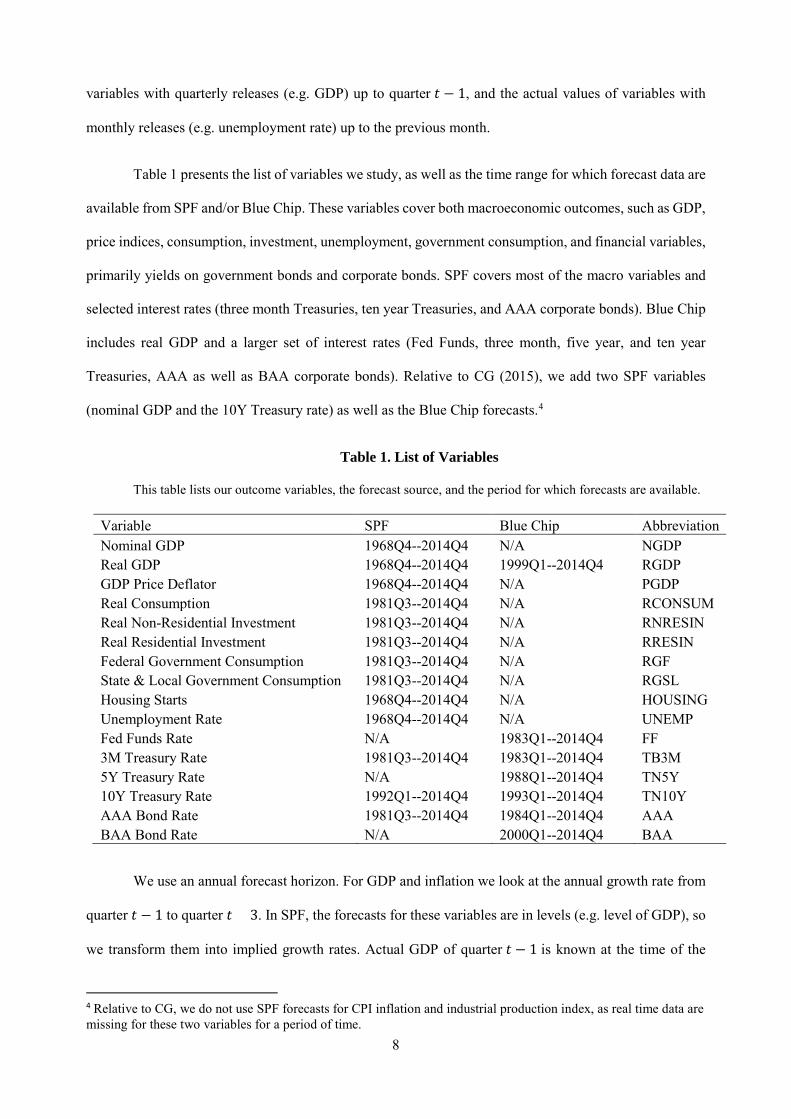
Table 1 presents the list of variables we study, as well as the time range for which forecast data are

available from SPF and/or Blue Chip. These variables cover both macroeconomic outcomes, such as GDP,

price indices, consumption, investment, unemployment, government consumption, and financial variables,

primarily yields on government bonds and corporate bonds. SPF covers most of the macro variables and

selected interest rates (three month Treasuries, ten year Treasuries, and AAA corporate bonds). Blue Chip

includes real GDP and a larger set of interest rates (Fed Funds, three month, five year, and ten year

Treasuries, AAA as well as BAA corporate bonds). Relative to CG (2015), we add two SPF variables

(nominal GDP and the 10Y Treasury rate) as well as the Blue Chip forecasts.4

Table 1. List of Variables

This table lists our outcome variables, the forecast source, and the period for which forecasts are available.

Variable SPF Blue Chip Abbreviation Nominal GDP 1968Q4--2014Q4 N/A NGDP Real GDP 1968Q4--2014Q4 1999Q1--2014Q4 RGDP GDP Price Deflator 1968Q4--2014Q4 N/A PGDP Real Consumption 1981Q3--2014Q4 N/A RCONSUM Real Non-Residential Investment 1981Q3--2014Q4 N/A RNRESIN Real Residential Investment 1981Q3--2014Q4 N/A RRESIN Federal Government Consumption 1981Q3--2014Q4 N/A RGF State & Local Government Consumption 1981Q3--2014Q4 N/A RGSL Housing Starts 1968Q4--2014Q4 N/A HOUSING Unemployment Rate 1968Q4--2014Q4 N/A UNEMP Fed Funds Rate N/A 1983Q1--2014Q4 FF 3M Treasury Rate 1981Q3--2014Q4 1983Q1--2014Q4 TB3M 5Y Treasury Rate N/A 1988Q1--2014Q4 TN5Y 10Y Treasury Rate 1992Q1--2014Q4 1993Q1--2014Q4 TN10Y AAA Bond Rate 1981Q3--2014Q4 1984Q1--2014Q4 AAA BAA Bond Rate N/A 2000Q1--2014Q4 BAA

We use an annual forecast horizon. For GDP and inflation we look at the annual growth rate from

quarter 𝑡𝑡 − 1 to quarter 𝑡𝑡 + 3. In SPF, the forecasts for these variables are in levels (e.g. level of GDP), so

we transform them into implied growth rates. Actual GDP of quarter 𝑡𝑡 − 1 is known at the time of the

4 Relative to CG, we do not use SPF forecasts for CPI inflation and industrial production index, as real time data are missing for these two variables for a period of time.

9

forecast, consistent with the forecasters’ information sets. Blue Chip reports forecasts of quarterly growth

rates, so we add up these forecasts in quarters 𝑡𝑡 to 𝑡𝑡 + 3. For variables such as the unemployment rate and

interest rates, we look at the level in quarter 𝑡𝑡 + 3. Both SPF and Blue Chip have direct forecasts of the

quarterly average level in quarter 𝑡𝑡 + 3. Appendix B provides a description of variable construction.

Consensus forecasts are computed as means from individual-level forecasts available at a point in

time. We calculate forecasts, forecast errors, and forecast revisions at the individual level, and then average

them across forecasters to compute the consensus.5

Data on Actual Outcomes. The values of macroeconomic variables are released quarterly but are often

subsequently revised. To match as closely as possible the forecasters’ information set, we focus on initial

releases from Philadelphia Fed’s Real-Time Data Set for Macroeconomists.6 For example, for actual GDP

growth from quarter 𝑡𝑡 − 1 to quarter 𝑡𝑡 + 3, we use the initial release of GDP𝑡𝑡+3 (available in quarter 𝑡𝑡 +

4) divided by the initial release of GDP𝑡𝑡−1 (available in quarter 𝑡𝑡, prior to when the forecasts are made).

For financial variables, the actual outcomes are available daily and are permanent (not revised). We use

historical data from the Federal Reserve Bank of St. Louis. In addition, we always study the properties of

the actuals (mean, standard deviation, persistence, etc) using the same time periods as the corresponding

forecasts. The same variable from SPF and Blue Chip may have slightly different actuals when the two

datasets cover different time periods.

Summary Statistics. Table 2 below presents the summary statistics of the variables, including the mean and

standard deviation for the actuals being forecasted, as well as the consensus forecasts, forecast errors, and

forecast revisions at a horizon of quarter t+3. The table also shows statistics for the quarterly share of

forecasters with no meaningful revisions,7 and the quarterly share of forecasters with positive revisions.

5 There could be small differences in the set of forecasters who issue a forecast in quarter 𝑡𝑡, and those who revise their forecast at 𝑡𝑡 (these need to be present at 𝑡𝑡 − 1 as well). This issue does not affect our results, which are robust to considering only forecasters who have both forecasts and forecast revisions. 6 When forecasters make forecasts in quarter 𝑡𝑡, only initial releases of macro variables in quarter 𝑡𝑡 − 1 are available. 7 We categorize a forecaster as making no revision if he provides non-missing forecasts in both quarters 𝑡𝑡 − 1 and 𝑡𝑡, and the forecasts change by less than 0.01 percentage points. For variables in rates, the data is often rounded to the first decimal point, and this rounding may lead to a higher incidence of no-revision.

10

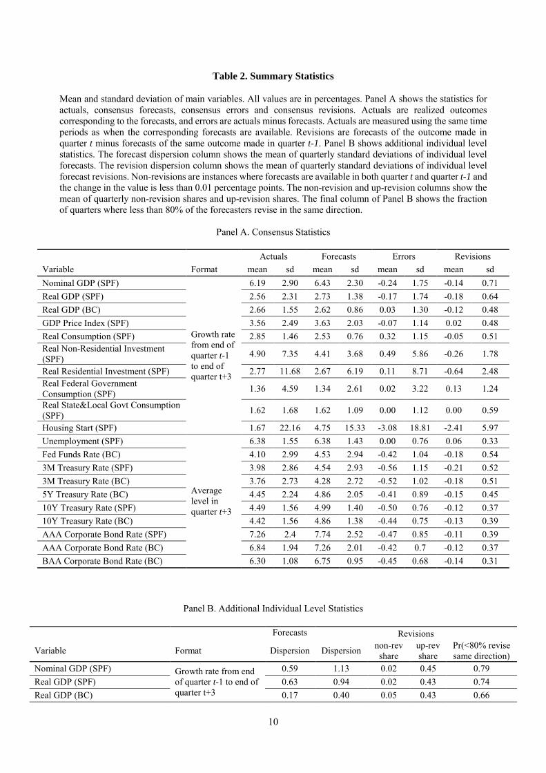
Table 2. Summary Statistics

Mean and standard deviation of main variables. All values are in percentages. Panel A shows the statistics for actuals, consensus forecasts, consensus errors and consensus revisions. Actuals are realized outcomes corresponding to the forecasts, and errors are actuals minus forecasts. Actuals are measured using the same time periods as when the corresponding forecasts are available. Revisions are forecasts of the outcome made in quarter t minus forecasts of the same outcome made in quarter t-1. Panel B shows additional individual level statistics. The forecast dispersion column shows the mean of quarterly standard deviations of individual level forecasts. The revision dispersion column shows the mean of quarterly standard deviations of individual level forecast revisions. Non-revisions are instances where forecasts are available in both quarter t and quarter t-1 and the change in the value is less than 0.01 percentage points. The non-revision and up-revision columns show the mean of quarterly non-revision shares and up-revision shares. The final column of Panel B shows the fraction of quarters where less than 80% of the forecasters revise in the same direction.

Panel A. Consensus Statistics

Actuals Forecasts Errors Revisions Variable Format mean sd mean sd mean sd mean sd Nominal GDP (SPF)

Growth rate from end of quarter t-1 to end of quarter t+3

6.19 2.90 6.43 2.30 -0.24 1.75 -0.14 0.71 Real GDP (SPF) 2.56 2.31 2.73 1.38 -0.17 1.74 -0.18 0.64 Real GDP (BC) 2.66 1.55 2.62 0.86 0.03 1.30 -0.12 0.48 GDP Price Index (SPF) 3.56 2.49 3.63 2.03 -0.07 1.14 0.02 0.48 Real Consumption (SPF) 2.85 1.46 2.53 0.76 0.32 1.15 -0.05 0.51 Real Non-Residential Investment (SPF) 4.90 7.35 4.41 3.68 0.49 5.86 -0.26 1.78

Real Residential Investment (SPF) 2.77 11.68 2.67 6.19 0.11 8.71 -0.64 2.48 Real Federal Government Consumption (SPF) 1.36 4.59 1.34 2.61 0.02 3.22 0.13 1.24

Real State&Local Govt Consumption (SPF) 1.62 1.68 1.62 1.09 0.00 1.12 0.00 0.59

Housing Start (SPF) 1.67 22.16 4.75 15.33 -3.08 18.81 -2.41 5.97 Unemployment (SPF)

Average level in quarter t+3

6.38 1.55 6.38 1.43 0.00 0.76 0.06 0.33 Fed Funds Rate (BC) 4.10 2.99 4.53 2.94 -0.42 1.04 -0.18 0.54 3M Treasury Rate (SPF) 3.98 2.86 4.54 2.93 -0.56 1.15 -0.21 0.52 3M Treasury Rate (BC) 3.76 2.73 4.28 2.72 -0.52 1.02 -0.18 0.51 5Y Treasury Rate (BC) 4.45 2.24 4.86 2.05 -0.41 0.89 -0.15 0.45 10Y Treasury Rate (SPF) 4.49 1.56 4.99 1.40 -0.50 0.76 -0.12 0.37 10Y Treasury Rate (BC) 4.42 1.56 4.86 1.38 -0.44 0.75 -0.13 0.39 AAA Corporate Bond Rate (SPF) 7.26 2.4 7.74 2.52 -0.47 0.85 -0.11 0.39 AAA Corporate Bond Rate (BC) 6.84 1.94 7.26 2.01 -0.42 0.7 -0.12 0.37 BAA Corporate Bond Rate (BC) 6.30 1.08 6.75 0.95 -0.45 0.68 -0.14 0.31

Panel B. Additional Individual Level Statistics

Forecasts Revisions

Variable Format Dispersion Dispersion non-rev share

up-rev share

Pr(<80% revise same direction)

Nominal GDP (SPF) Growth rate from end of quarter t-1 to end of quarter t+3

0.59 1.13 0.02 0.45 0.79 Real GDP (SPF) 0.63 0.94 0.02 0.43 0.74 Real GDP (BC) 0.17 0.40 0.05 0.43 0.66

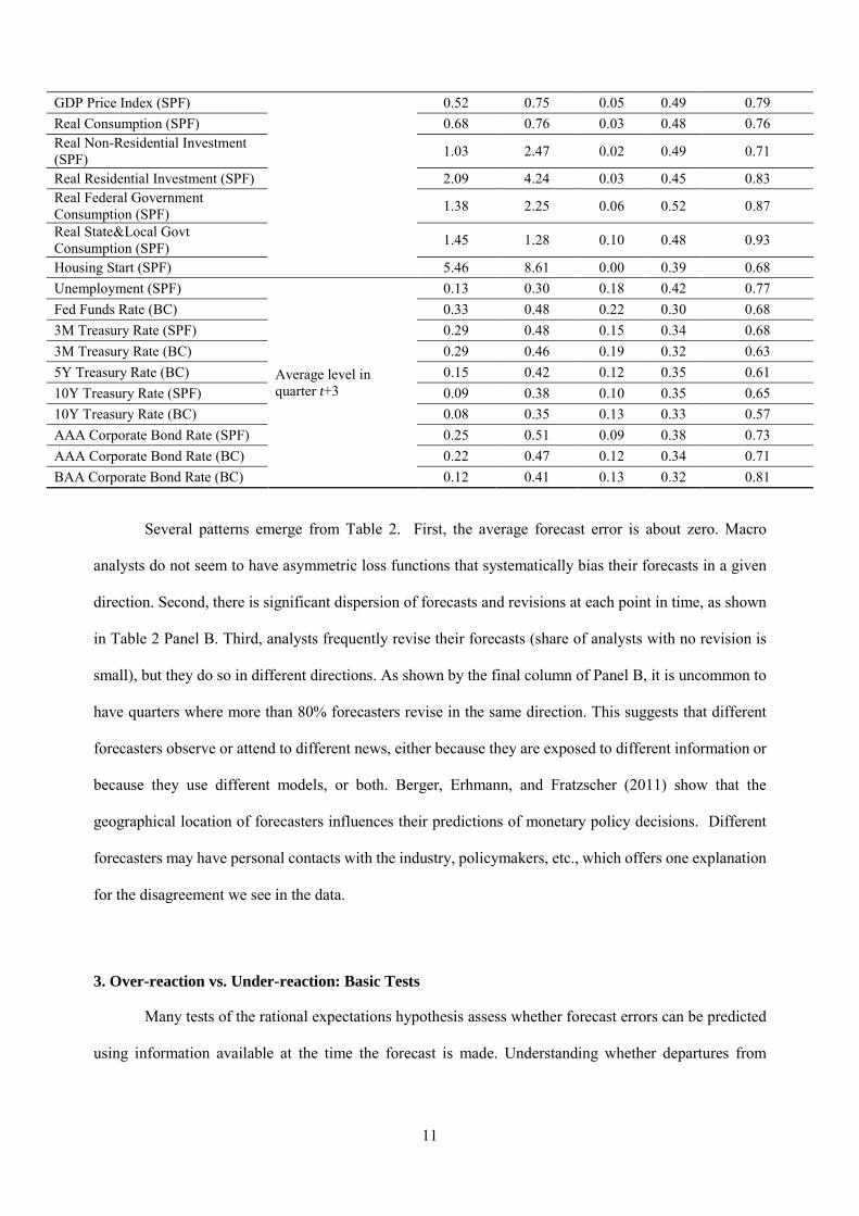
11

GDP Price Index (SPF) 0.52 0.75 0.05 0.49 0.79 Real Consumption (SPF) 0.68 0.76 0.03 0.48 0.76 Real Non-Residential Investment (SPF) 1.03 2.47 0.02 0.49 0.71

Real Residential Investment (SPF) 2.09 4.24 0.03 0.45 0.83 Real Federal Government Consumption (SPF) 1.38 2.25 0.06 0.52 0.87

Real State&Local Govt Consumption (SPF) 1.45 1.28 0.10 0.48 0.93

Housing Start (SPF) 5.46 8.61 0.00 0.39 0.68 Unemployment (SPF)

Average level in quarter t+3

0.13 0.30 0.18 0.42 0.77 Fed Funds Rate (BC) 0.33 0.48 0.22 0.30 0.68 3M Treasury Rate (SPF) 0.29 0.48 0.15 0.34 0.68 3M Treasury Rate (BC) 0.29 0.46 0.19 0.32 0.63 5Y Treasury Rate (BC) 0.15 0.42 0.12 0.35 0.61 10Y Treasury Rate (SPF) 0.09 0.38 0.10 0.35 0.65 10Y Treasury Rate (BC) 0.08 0.35 0.13 0.33 0.57 AAA Corporate Bond Rate (SPF) 0.25 0.51 0.09 0.38 0.73 AAA Corporate Bond Rate (BC) 0.22 0.47 0.12 0.34 0.71 BAA Corporate Bond Rate (BC) 0.12 0.41 0.13 0.32 0.81

Several patterns emerge from Table 2. First, the average forecast error is about zero. Macro

analysts do not seem to have asymmetric loss functions that systematically bias their forecasts in a given

direction. Second, there is significant dispersion of forecasts and revisions at each point in time, as shown

in Table 2 Panel B. Third, analysts frequently revise their forecasts (share of analysts with no revision is

small), but they do so in different directions. As shown by the final column of Panel B, it is uncommon to

have quarters where more than 80% forecasters revise in the same direction. This suggests that different

forecasters observe or attend to different news, either because they are exposed to different information or

because they use different models, or both. Berger, Erhmann, and Fratzscher (2011) show that the

geographical location of forecasters influences their predictions of monetary policy decisions. Different

forecasters may have personal contacts with the industry, policymakers, etc., which offers one explanation

for the disagreement we see in the data.

3. Over-reaction vs. Under-reaction: Basic Tests

Many tests of the rational expectations hypothesis assess whether forecast errors can be predicted

using information available at the time the forecast is made. Understanding whether departures from

12

rational expectations are due to over- or under-reaction to information is more challenging, since the

forecaster’s full information set cannot be directly observed by the econometrician.

CG (2015) address this problem with forecast revisions. Denote by 𝑥𝑥𝑡𝑡+ℎ|𝑡𝑡 the ℎ-periods ahead

forecast made at time 𝑡𝑡 about the future value 𝑥𝑥𝑡𝑡+ℎ of a variable. Denote by 𝑥𝑥𝑡𝑡+ℎ|𝑡𝑡−1 the forecast of the

same variable in the previous period. The ℎ-periods ahead forecast revision at 𝑡𝑡 is given by 𝐹𝐹𝑅𝑅𝑡𝑡,ℎ =

�𝑥𝑥𝑡𝑡+ℎ|𝑡𝑡 − 𝑥𝑥𝑡𝑡+ℎ|𝑡𝑡−1�, or the one period change in the forecast about 𝑥𝑥𝑡𝑡+ℎ. This revision captures the

reaction to whichever news the forecasters have observed. The extent to which forecasters under- or over-

react to information can then be assessed by estimating the regression:

𝑥𝑥𝑡𝑡+ℎ − 𝑥𝑥𝑡𝑡+ℎ|𝑡𝑡 = 𝛽𝛽0 + 𝛽𝛽1𝐹𝐹𝑅𝑅𝑡𝑡,ℎ + 𝜖𝜖𝑡𝑡,𝑡𝑡+ℎ . (1)

Under the Rational Expectations Hypothesis, the forecast error should be unpredictable using any

current information, including the forecast revision itself, so 𝛽𝛽1 = 0. When instead the forecast under-

reacts to information, we expect 𝛽𝛽1 > 0. To see why, suppose that positive information is received, leading

to a positive forecast revision 𝐹𝐹𝑅𝑅𝑡𝑡,ℎ > 0. If the forecast under-reacts, the upward revision is insufficient,

predicting a positive forecast error 𝔼𝔼𝑡𝑡�𝑥𝑥𝑡𝑡+ℎ − 𝑥𝑥𝑡𝑡+ℎ|𝑡𝑡� > 0. The converse holds if negative information is

received: the downward revision is insufficient, predicting a negative error. Under-reaction implies that

the forecast error should be positively correlated with the forecast revision.

By the same logic, when the forecast over-reacts to information we should expect 𝛽𝛽1 < 0. Indeed,

over-reaction means that after positive information 𝐹𝐹𝑅𝑅𝑡𝑡,ℎ > 0 the forecast is too optimistic, so the forecast

error is negative 𝔼𝔼𝑡𝑡�𝑥𝑥𝑡𝑡+ℎ − 𝑥𝑥𝑡𝑡+ℎ|𝑡𝑡� < 0. On the other hand, after negative information 𝐹𝐹𝑅𝑅𝑡𝑡,ℎ < 0 it is too

pessimistic, so the error is positive 𝔼𝔼𝑡𝑡�𝑥𝑥𝑡𝑡+ℎ − 𝑥𝑥𝑡𝑡+ℎ|𝑡𝑡� > 0. That is, over-reaction implies that the forecast

error should be negatively correlated with the forecast revision.

To test for Rational Inattention, CG’s baseline estimate of Equation (1) uses consensus SPF

forecasts. The consensus forecast 𝑥𝑥𝑡𝑡+ℎ|𝑡𝑡 is defined as the average of individual forecasters’ predictions

𝑥𝑥𝑡𝑡+ℎ|𝑡𝑡 = 1𝐼𝐼∑ 𝑥𝑥𝑡𝑡+ℎ|𝑡𝑡

𝑖𝑖 𝑖𝑖 , where 𝐼𝐼 > 1 is the number of forecasters. Similarly, 𝐹𝐹𝑅𝑅𝑡𝑡,ℎ is the ℎ-periods ahead

13

“consensus information” or forecast revision. CG estimate (1) for the GDP price deflator (PGDP_SPF) at

a horizon ℎ = 3 and find 𝛽𝛽1 = 1.2, which is robust to a number of controls. They also run Equation (1)

for 13 SPF variables by pooling forecast horizons from ℎ = 0 to ℎ = 3, and find qualitatively similar

results, with 8 out of 13 variables exhibiting significantly positive 𝛽𝛽1’s and the average coefficient being

close to 0.7 (see Figure 1 Panel B of CG (2015)). The general message is that consensus forecasts of

macroeconomic variables display under-reaction.

We estimate Equation (1) for our 20 series for the same baseline horizon ℎ = 3, using consensus

forecasts. Standard errors are Newey-West with the automatic bandwidth selection following Newey and

West (1994). 8 The results are reported in columns (1) through (3) of Table 3, and confirm the findings of

CG. The estimated 𝛽𝛽1 is positive for 14 out of 20 series, statistically significant for 8 of them at the 5%

confidence level, and for a further two series at the 10% level (and our point estimate for inflation forecasts

coincides with CG’s). While results for the other SPF series are not directly comparable (since CG pool

across forecast horizons), the estimates lie in a similar range. The one exception is RGF_SPF (federal

government spending) for which the estimated 𝛽𝛽1 is negative and significant at the 5% level. Results from

the Blue Chip survey align well with SPF where they overlap, but do not exhibit significant consensus

over-reaction for the remaining (exclusively financial variables) series.

We stress that the various forecast series are not independent. For instance, nominal and real GDP

growth are highly correlated; the different interest rate series are also closely connected. Nonetheless, the

general message holds: for macro variables and short rates, under-reaction is common in the consensus

forecast regressions, while such patterns are largely absent in long-term rates.

As mentioned above, insufficient updating of consensus beliefs may be due to aggregation issues,

rather than to under-reaction to information by individual forecasters. As we saw in Table 2, individual

8 We also perform sensitivity analysis on the kernel bandwidth selection for Newey-West standard errors. In Appendix C Table C.1, we present standard errors using lags from zero to eight, which cover the reasonable range given the length of our time series. The results are largely similar.

14

forecasters often revise in different directions, perhaps because they look at different data or use different

models. Over-reaction of individual forecasters may thus be attenuated by heterogeneity and aggregation.

Table 3. Error-on-Revision Regression Results

This table shows coefficients from the CG (forecast error on forecast revision) regression. Coefficients are displayed for both consensus time-series regressions, and forecaster-level pooled panel regressions, together with standard errors and p-values. Standard errors are Newey-West for consensus time-series regressions, and clustered by both forecaster and time for individual level regressions.

Consensus Individual No fixed effects With fixed effects 𝛽𝛽1 s.e. p-val 𝛽𝛽1

𝑝𝑝 s.e. p-val 𝛽𝛽1𝑝𝑝 s.e. p-val

Variable (1) (2) (3) (4) (5) (6) (7) (8) (9) Nominal GDP (SPF) 0.48 0.22 0.03 -0.26 0.07 0.00 -0.30 0.06 0.00 Real GDP (SPF) 0.45 0.25 0.07 -0.23 0.08 0.00 -0.21 0.06 0.00 Real GDP (BC) 0.59 0.34 0.09 0.12 0.19 0.26 -0.02 0.17 0.93 GDP Price Index Inflation (SPF) 1.21 0.21 0.00 -0.07 0.10 0.46 -0.16 0.07 0.03 Real Consumption (SPF) 0.18 0.22 0.41 -0.34 0.11 0.00 -0.39 0.10 0.00 Real Non-Residential Investment (SPF) 0.93 0.38 0.02 0.01 0.13 0.93 -0.03 0.12 0.82 Real Residential Investment (SPF) 1.26 0.38 0.00 -0.02 0.10 0.82 -0.12 0.08 0.14 Real Federal Government Consumption (SPF) -0.44 0.23 0.05 -0.62 0.07 0.00 -0.63 0.06 0.00 Real State & Local Govt Consumption (SPF) -0.16 0.20 0.42 -0.71 0.14 0.00 -0.73 0.13 0.00 Housing Start (SPF) 0.45 0.31 0.14 -025 0.09 0.01 -0.28 0.08 0.00 Unemployment (SPF) 0.82 0.21 0.00 0.33 0.11 0.00 0.26 0.11 0.02 Fed Funds Rate (BC) 0.61 0.23 0.01 0.15 0.09 0.11 0.12 0.09 0.19 3M Treasury Rate (SPF) 0.71 0.26 0.01 0.24 0.09 0.01 0.19 0.09 0.04 3M Treasury Rate (BC) 0.67 0.25 0.01 0.20 0.09 0.02 0.16 0.08 0.06 5Y Treasury Rate (BC) 0.05 0.22 0.84 -0.12 0.10 0.23 -0.19 0.10 0.05 10Y Treasury Rate (SPF) -0.01 0.28 0.97 -0.18 0.10 0.06 -0.23 0.09 0.01 10Y Treasury Rate (BC) -0.06 0.25 0.81 -0.17 0.12 0.14 -0.25 0.11 0.02 AAA Corporate Bond Rate (SPF) -0.01 0.24 0.97 -0.21 0.08 0.00 -0.26 0.07 0.00 AAA Corporate Bond Rate (BC) 0.21 0.21 0.31 -0.17 0.07 0.00 -0.22 0.06 0.00 BAA Corporate Bond Rate (BC) -0.14 0.28 0.62 -0.28 0.10 0.00 -0.34 0.10 0.00

To assess whether individual forecasters over- or under-react to their own information, we continue

to follow the CG methodology, but perform the analysis at the individual analyst level. Here 𝐹𝐹𝑅𝑅𝑡𝑡,ℎ𝑖𝑖 =

�𝑥𝑥𝑡𝑡+ℎ|𝑡𝑡𝑖𝑖 − 𝑥𝑥𝑡𝑡+ℎ|𝑡𝑡−1

𝑖𝑖 � is the analyst-level revision, and the ℎ-periods ahead individual forecast error is

𝑥𝑥𝑡𝑡+ℎ − 𝑥𝑥𝑡𝑡+ℎ|𝑡𝑡𝑖𝑖 . For each variable, we then pool all analysts and estimate the regression:

𝑥𝑥𝑡𝑡+ℎ − 𝑥𝑥𝑡𝑡+ℎ|𝑡𝑡𝑖𝑖 = 𝛽𝛽0

𝑝𝑝 + 𝛽𝛽1𝑝𝑝𝐹𝐹𝑅𝑅𝑡𝑡,ℎ

𝑖𝑖 + 𝜖𝜖𝑡𝑡,𝑡𝑡+ℎ𝑖𝑖 . (2)

15

Superscript 𝑝𝑝 on the coefficients recognizes that we are pooling individual level data. The logic of the test,

however, does not change: 𝛽𝛽1𝑝𝑝 > 0 indicates that the average analyst under-reacts to his own information,

while 𝛽𝛽1𝑝𝑝 < 0 indicates that the average analyst over-reacts.9

Columns (4) through (6) of Table 3 report the results of estimating Equation (2). Surprisingly, the

picture is essentially reversed from the consensus: at the individual level, the average analyst appears to

over-react to information, as measured by a negative 𝛽𝛽1𝑝𝑝 coefficient. The estimated 𝛽𝛽1

𝑝𝑝 is negative for 14

out of the 20 series (13 out of 16 variables), and significantly negative for 9 series at the 5% confidence

level, and for one other series at the 10% level. Except for short rates (Fed Funds and 3-months T-bill rate),

all financial variables display over-reaction, consistent with Shiller’s evidence of excess volatility. But

many macro variables also display over-reaction, including nominal GDP, real GDP (in SPF, not in Blue

Chip), real consumption, real federal government expenditures, real state and local government

expenditures. GDP price deflator inflation, real GDP in Blue Chip, and non-residential investment display

neither over-nor under-reaction (𝛽𝛽1𝑝𝑝 close to zero). Only the 3-months T-bill rate and unemployment rate

display individual level under-reaction with positive and statistically significant 𝛽𝛽1𝑝𝑝.

In columns (7) to (9), we also analyze regressions with forecaster fixed effects to account for

possible time-invariant differences among analysts. Some analysts may be consistently overly-optimistic

or overly-pessimistic, perhaps due to differences in their prior beliefs, contributing to positive correlations

between forecast errors and revisions. Specifically, the overly optimistic analysts systematically receive

bad news, leading to negative revisions and negative forecast errors, while the overly pessimistic analysts

systematically receive good news, leading to positive revisions and positive forecast errors. In the data, the

results with and without forecaster fixed effects are similar. With forecaster fixed effects, the estimated 𝛽𝛽1𝑝𝑝

is negative for 17 series, and significantly negative for 13 series at the 5% confidence level. The message

of Table 3 is clear: at the level of the individual forecaster, over-reaction is the norm.

9 The individual level coefficient 𝛽𝛽1

𝑝𝑝 can in principle be different from the consensus coefficient 𝛽𝛽1: to the extent that some information is forecaster specific, and that individuals do not react to information they do not possess, errors 𝜖𝜖𝑡𝑡,𝑡𝑡+ℎ𝑖𝑖 may be correlated across individuals over time. In Section 4 we formalize this intuition.

16

In sum, a fascinating picture emerges from these tests. At the consensus level, expectations

typically under-react. At the individual level, they typically over-react. We conclude this section with a

number of robustness checks. In Section 4, we present a model capable of reconciling these patterns.

3.1 Robustness Checks

Predictability of forecast errors might arise from features of the data unrelated to individuals’

under- or over-reaction to news. We next show that our results are robust to many such confounds.

Small Samples. Our individual level estimates can face small sample problems. Finite-sample biases exist

in time series regressions (Kendall 1954, Stambaugh 1999) and panel regressions with fixed effects

(Nickell, 1981). In the baseline individual-level tests in Table 3, our panel regressions do not have fixed

effects, which alleviates the concern (Hjalmarsson 2008). Adding fixed effects does not change the results

much, indicating that the bias, even if present, is not severe. Moreover, the finite sample biases are stronger

when the predictor variables are persistent. The predictor variable in the CG regressions, namely forecast

revision, has low persistence in the data (about zero for most variables at the individual level, and less than

0.5 at the consensus level). Finally, simulation analyses in Appendix D show that, for parameter values

and time frames relevant to our data, the coefficients do not have notable biases.

Measurement Error. Forecasts measured with noise can mechanically lead to negative predictability of

forecast errors in Equation (2): a positive shock increases the measured forecast revision and decreases the

forecast error. In our case, since professional forecasters directly report their forecasts, it is hard to think

of literal “measurement error.” Moreover, motivated by the fact that some series display an AR(2)

structure, in Section 5 we regress the forecast error at 𝑡𝑡 + ℎ on revisions of forecasts for previous periods

𝑡𝑡 + ℎ − 1 and 𝑡𝑡 + ℎ − 2 (Equation 13). In line with the predictions of the model (Proposition 3), but not

with measurement error, we find strong predictability in these regressions as well (Table 6). Finally, in

Section 6 we estimate our model without using information from the CG coefficients; we obtain estimates

that indicate significant individual level over-reaction and generate CG regression coefficients very similar

to the data.

17

Heterogeneity among Forecasters. Forecaster heterogeneity either in updating (e.g., heterogeneous signal

to noise ratios), or in beliefs about long term means, may affect the predictability of forecast errors. To

assess this problem, we perform forecaster level regressions, focusing on forecasters with at least 10

observations. Table C2 in Appendix C compares the median coefficient from forecaster level regressions

to the coefficients from pooled individual level regressions from Table 3. The coefficients are very similar,

so the observed over-reaction describes the median forecaster. On average across series, we estimate a

negative 𝛽𝛽1𝑝𝑝 for two thirds of the forecasters. In some series, nearly every forecaster over-reacts while in

other series the distribution of 𝛽𝛽1𝑝𝑝s is more balanced. We return to forecaster heterogeneity in Section 6,

when we estimate our model.

Asymmetric Loss Functions. Another concern with our findings is that forecast errors reflect not cognitive

limitations but analysts’ biased incentives. Of course, an analyst’s objective is difficult to observe. Here

we discuss the implications of several analyst loss functions proposed in the literature.

With an asymmetric loss function (Capistran and Timmerman 2009), the over-reaction pattern in

Table 3 may be generated by a combination of: i) a higher cost of over- than under-predicting, and ii)

suitably time varying volatility (Pesaran and Weale 2006). In this case, an asymmetric loss function would

also generate an average forecast error in the form of pessimism. In the data, however, forecasts are not

systematically upward or downward biased on average. The consensus forecast errors are small and

insignificant (Table 2, panel A). This is also true for individual forecast errors: we fail to reject that the

average error is different from zero for about 60% of forecasters for the macroeconomic variables.10

Another source of bias in reported expectations is that individuals may follow consensus forecasts

(Morris and Shin 2002, Fuhrer 2017). Let 𝑥𝑥�𝑡𝑡+ℎ|𝑡𝑡𝑖𝑖 = 𝛼𝛼𝑥𝑥𝑡𝑡+ℎ|𝑡𝑡

𝑖𝑖 + (1 − 𝛼𝛼)𝑥𝑥�𝑡𝑡+ℎ|𝑡𝑡 , where 𝑥𝑥𝑡𝑡+ℎ|𝑡𝑡𝑖𝑖 is the

individual rational forecast and 𝑥𝑥�𝑡𝑡+ℎ|𝑡𝑡 is the average contemporaneous forecast with this bias (which

coincides with the consensus without this bias). Our benchmark model has 𝛼𝛼 = 1 but for 𝛼𝛼 < 1 forecasters

put weight on others’ signals at the expense of their own. In this model, in line with intuition, following

10 Some individual forecasters have average errors that are significantly different from zero for some series, but these average out in the population for nearly all series. For interest rates, average forecast errors tend to be negative, but this reflects the secular decline in rates over the time period we examine.

18

consensus forecasts leads to individual level under-reaction, namely positive individual level CG

coefficients, contrary to our findings.11

Reputational incentives may also induce forecast smoothing. In response to news at 𝑡𝑡, forecasters

may wish to minimize forecast revisions by taking into account the previous forecast 𝑥𝑥𝑡𝑡+ℎ|𝑡𝑡−1𝑖𝑖 as well as

the future path 𝑥𝑥𝑡𝑡+ℎ|𝑡𝑡+𝑗𝑗𝑖𝑖 . To assess the relevance of this mechanism, note that forecast smoothing should

reduce the current revision for the current quarter (ℎ = 0), creating under-reaction. This prediction is

contradicted by the data: negative predictability prevails even at this horizon (Appendix C, Table C3).

More generally, the similarity of our results across datasets suggests that distorted incentives

cannot be the whole story. The SPF panelists are anonymous, the Blue Chip ones are not. Thus, forecasts

in Blue Chip should be more affected by the above reputational incentives or by additional ones (e.g.,

individual forecasters may wish to distinguish themselves from others in order to prevail in a winner-take-

all context, as in Ottaviani and Sorensen (2006)). However, in our data, when Blue Chip and SPF forecasts

are available for the same series, they display very similar average forecast errors and revisions (see Table

2), they have similar CG coefficients (see Table 3), and they lead to similar model estimates (see Section

6). Analyst incentives do not seem a compelling explanation for our findings.

Fat tailed shocks. In our data both fundamentals and forecast revisions have high kurtosis. To see whether

fat tailed shocks may, by themselves, create a false impression of over-reaction, in Appendix D we consider

a learning setting with fat tailed fundamental shocks. Without normality, we can no longer use the Kalman

filter, but instead need to use the particle filter (Liu and Chen, 1998; Doucet, de Freitas, and Gordon, 2001).

We find that when forecasts are produced using the particle filter under rational expectations, individual

forecast errors are not predictable from forecast revisions, and thus cannot explain the evidence. Moreover,

in Section 6 we estimate a modified particle filter that allows for overreaction to news, and find that fat

11 Formally, denote 𝐹𝐹𝐹𝐹�𝑡𝑡+ℎ,𝑡𝑡

𝑖𝑖 = 𝑥𝑥𝑡𝑡+ℎ − 𝑥𝑥�𝑡𝑡+ℎ|𝑡𝑡𝑖𝑖 the forecast error and 𝐹𝐹𝑅𝑅�𝑡𝑡+ℎ,𝑡𝑡

𝑖𝑖 = 𝑥𝑥�𝑡𝑡+ℎ|𝑡𝑡𝑖𝑖 − 𝑥𝑥�𝑡𝑡+ℎ|𝑡𝑡−1

𝑖𝑖 the forecast revision. It follows that 𝐹𝐹𝐹𝐹�𝑡𝑡+ℎ,𝑡𝑡

𝑖𝑖 = 𝛼𝛼𝐹𝐹𝐹𝐹𝑡𝑡+ℎ,𝑡𝑡𝑖𝑖 + (1 − 𝛼𝛼)𝐹𝐹𝐹𝐹𝑡𝑡+ℎ|𝑡𝑡 and similarly 𝐹𝐹𝑅𝑅�𝑡𝑡+ℎ,𝑡𝑡

𝑖𝑖 = 𝛼𝛼𝐹𝐹𝑅𝑅𝑡𝑡+ℎ,𝑡𝑡𝑖𝑖 + (1 − 𝛼𝛼)𝐹𝐹𝑅𝑅𝑡𝑡+ℎ|𝑡𝑡 . Then

𝑐𝑐𝑐𝑐𝑐𝑐�𝐹𝐹𝐹𝐹�𝑡𝑡+ℎ,𝑡𝑡𝑖𝑖 ,𝐹𝐹𝑅𝑅�𝑡𝑡+ℎ,𝑡𝑡

𝑖𝑖 � > 0 follows from 𝑐𝑐𝑐𝑐𝑐𝑐�𝐹𝐹𝐹𝐹𝑡𝑡+ℎ,𝑡𝑡𝑖𝑖 ,𝐹𝐹𝑅𝑅𝑡𝑡+ℎ,𝑡𝑡

𝑖𝑖 � = 0 and 𝑐𝑐𝑐𝑐𝑐𝑐�𝐹𝐹𝐹𝐹𝑡𝑡+ℎ|𝑡𝑡 ,𝐹𝐹𝑅𝑅𝑡𝑡+ℎ|𝑡𝑡� > 0 under noisy rational expectations, together with 𝑐𝑐𝑐𝑐𝑐𝑐�𝐹𝐹𝐹𝐹𝑡𝑡+ℎ,𝑡𝑡

𝑖𝑖 ,𝐹𝐹𝑅𝑅𝑡𝑡+ℎ|𝑡𝑡�, 𝑐𝑐𝑐𝑐𝑐𝑐�𝐹𝐹𝐹𝐹𝑡𝑡+ℎ|𝑡𝑡 ,𝐹𝐹𝑅𝑅𝑡𝑡+ℎ,𝑡𝑡𝑖𝑖 � > 0.

19

tailed shocks do not significantly affect our quantitative estimates. Because fat tails do not appear to affect

our results, we maintain the more tractable assumption of normality in our theoretical analysis.12

4. Diagnostic Expectations

We present a model that reconciles under-reaction of consensus expectations with over-reaction of

individual level expectations. At each time 𝑡𝑡, the target of forecasts is a hidden state 𝑥𝑥𝑡𝑡+ℎ whose current

value 𝑥𝑥𝑡𝑡 is not directly observed. What is observed instead is a noisy signal 𝑠𝑠𝑡𝑡𝑖𝑖:

𝑠𝑠𝑡𝑡𝑖𝑖 = 𝑥𝑥𝑡𝑡 + 𝜖𝜖𝑡𝑡𝑖𝑖 , (3)

where 𝜖𝜖𝑡𝑡𝑖𝑖 is noise, i.i.d. normally distributed across forecasters and over time, with mean zero and variance

𝜎𝜎𝜖𝜖2. The hidden state 𝑥𝑥𝑡𝑡 evolves according to an AR(1) process with persistence 𝜌𝜌:

𝑥𝑥𝑡𝑡 = 𝜌𝜌𝑥𝑥𝑡𝑡−1 + 𝑢𝑢𝑡𝑡 , (4)

where 𝑢𝑢𝑡𝑡 is a normal shock with mean zero and variance 𝜎𝜎𝑢𝑢2. This AR(1) setting, also considered by CG

(2015), yields convenient closed form predictions. In Section 6 we examine the AR(2) case.

This setup accommodates several interpretations. In CG (2015), unobservability of 𝑥𝑥𝑡𝑡 stems from

rational inattention (Sims 2003, Woodford 2003). Forecasters could in principle observe 𝑥𝑥𝑡𝑡 but doing so

is too costly, so they observe a noisy proxy for it and optimally use that proxy in their forecasts.13 This

rational inattention interpretation is not entirely convincing, since the job of professional forecasters is

precisely to be attentive to, and to predict, the variables in question.

A more compelling story is that forecasters observe the same data, say GDP or interest rates, but

differ in their interpretations because they have different pieces of other information. Think of the current

GDP estimate or interest rate level as a noisy proxy for an unobservable persistent state. Due to individual

12 Apart from fat tails, skewness of shocks may also lead to systematically biased forecasts under Bayesian updating (Orlik and Veldkamp 2015). As we saw in Table 2, in our data forecasts are not biased on average. 13 As CG show, the same predictions are obtained if rational inattention is modelled à la Mankiw and Reis (2002), where agents observe the same information but only sporadically revise their predictions.

20

expertise or contacts in the industry, a forecaster has personal information on that hidden state. This

implies that the current GDP estimate or interest rate level is transformed into a forecaster-specific signal

𝑠𝑠𝑡𝑡𝑖𝑖. Even so, a Bayesian forecaster optimally filters noise in his own signal. In this sense, under both the

rational inattention and the dispersed information interpretations, forecasters rationally update on the basis

of noisy signals. We refer to both mechanisms as “Noisy Rational Expectations”.

A Bayesian, or rational, forecaster enters period 𝑡𝑡 carrying from the previous period beliefs about

the current state 𝑥𝑥𝑡𝑡 summarized by a probability density 𝑓𝑓�𝑥𝑥𝑡𝑡|𝑆𝑆𝑡𝑡−1𝑖𝑖 �, where 𝑆𝑆𝑡𝑡−1𝑖𝑖 denotes the full history of

signals observed by this forecaster.14 In period 𝑡𝑡, the forecaster observes a new signal 𝑠𝑠𝑡𝑡𝑖𝑖. In light of

this evidence, he updates his estimate of the current state using Bayes’ rule:

𝑓𝑓�𝑥𝑥𝑡𝑡|𝑆𝑆𝑡𝑡𝑖𝑖� =𝑓𝑓�𝑠𝑠𝑡𝑡𝑖𝑖|𝑥𝑥𝑡𝑡�𝑓𝑓�𝑥𝑥𝑡𝑡|𝑆𝑆𝑡𝑡−1𝑖𝑖 �∫ 𝑓𝑓�𝑠𝑠𝑡𝑡𝑖𝑖|𝑥𝑥�𝑓𝑓�𝑥𝑥|𝑆𝑆𝑡𝑡−1𝑖𝑖 �𝑑𝑑𝑥𝑥

. (5)

Equation (5) iteratively defines the forecaster’s beliefs. Given normal shocks, 𝑓𝑓�𝑥𝑥𝑡𝑡|𝑆𝑆𝑡𝑡𝑖𝑖� is

described by the Kalman filter. A rational forecaster estimates the current state at 𝑥𝑥𝑡𝑡|𝑡𝑡𝑖𝑖 = ∫𝑥𝑥𝑓𝑓�𝑥𝑥|𝑆𝑆𝑡𝑡𝑖𝑖�𝑑𝑑𝑥𝑥

and forecasts future values using the AR(1) structure, so 𝑥𝑥𝑡𝑡+ℎ|𝑡𝑡𝑖𝑖 = 𝜌𝜌ℎ𝑥𝑥𝑡𝑡|𝑡𝑡

𝑖𝑖 .

We allow beliefs to be distorted by Kahneman and Tversky’s representativeness heuristic, as in

our model of Diagnostic Expectations. In line with BGLS (2017), who apply Diagnostic Expectations to a

(diagnostic) Kalman Filter, we define the representativeness of a state 𝑥𝑥 at 𝑡𝑡 as the likelihood ratio:

𝑅𝑅𝑡𝑡(𝑥𝑥) =𝑓𝑓�𝑥𝑥|𝑆𝑆𝑡𝑡𝑖𝑖�

𝑓𝑓�𝑥𝑥|𝑆𝑆𝑡𝑡−1𝑖𝑖 ∪ �𝑥𝑥𝑡𝑡|𝑡𝑡−1𝑖𝑖 ��

. (6)

State 𝑥𝑥 is more representative at 𝑡𝑡 if the signal 𝑠𝑠𝑡𝑡𝑖𝑖 received in this period increases the probability of that

state, relative to not receiving any news. Receiving no news means observing a signal equal to the ex-ante

forecast, 𝑠𝑠𝑡𝑡𝑖𝑖 = 𝑥𝑥𝑡𝑡|𝑡𝑡−1𝑖𝑖 , as described in the denominator of equation (6).

14 Equation (5) assumes that forecasters observe only their individual signals. In reality they also observe common signals, such as public announcements and the past consensus of all other forecasters. In our analysis we focus on individual signals, which drive the difference between individual and consensus forecasts. We consider public signals in Corollary 1, and show that they do not alter the qualitative properties of the model.

21

Intuitively, the most representative states are those whose likelihood has increased the most in light

of recent data. The forecaster then overweighs representative states by using the distorted posterior:

𝑓𝑓𝜃𝜃�𝑥𝑥𝑡𝑡|𝑆𝑆𝑡𝑡𝑖𝑖� = 𝑓𝑓�𝑥𝑥𝑡𝑡|𝑆𝑆𝑡𝑡𝑖𝑖�𝑅𝑅𝑡𝑡(𝑥𝑥𝑡𝑡)𝜃𝜃1𝑍𝑍𝑡𝑡

, (7)

where 𝑍𝑍𝑡𝑡 is a normalization factor ensuring that 𝑓𝑓𝜃𝜃�𝑥𝑥𝑡𝑡|𝑆𝑆𝑡𝑡𝑖𝑖� integrates to one. Parameter 𝜃𝜃 ≥ 0 denotes the

extent to which beliefs are distorted by representativeness. For 𝜃𝜃 = 0 beliefs are rational, described by the

Bayesian conditional distribution 𝑓𝑓�𝑥𝑥𝑡𝑡|𝑆𝑆𝑡𝑡𝑖𝑖� . For 𝜃𝜃 > 0 the diagnostic density 𝑓𝑓𝜃𝜃�𝑥𝑥𝑡𝑡|𝑆𝑆𝑡𝑡𝑖𝑖� inflates the

probability of representative states and deflates the probability of unrepresentative ones. Mistakes occur

because states that have become relatively more likely may still be unlikely in absolute terms.

This formalization of representativeness as relative likelihood, and its effect on probability

assessments, has been shown to unify well-known laboratory biases in probability assessments such as

base rate neglect, the conjunction fallacy, and the disjunction fallacy (Gennaioli and Shleifer 2010). It has

also been used to explain real world phenomena such as stereotyping (BCGS 2016), self-confidence

(BCGS 2018), and expectation formation in financial markets (BGS 2018, BGLS 2017). Here we assess

whether this same structure can shed light on errors in forecasting macroeconomic variables.

Equation (7) yields a very intuitive characterization of beliefs.

Proposition 1 The distorted density 𝑓𝑓𝜃𝜃�𝑥𝑥𝑡𝑡|𝑆𝑆𝑡𝑡𝑖𝑖� is normal. In the steady state it is characterized by a

constant variance Σ𝜎𝜎𝜖𝜖2

Σ+𝜎𝜎𝜖𝜖2 and by a time varying mean 𝑥𝑥𝑡𝑡|𝑡𝑡

𝑖𝑖,𝜃𝜃 where:

𝑥𝑥𝑡𝑡|𝑡𝑡𝑖𝑖,𝜃𝜃 = 𝑥𝑥𝑡𝑡|𝑡𝑡−1

𝑖𝑖 + (1 + 𝜃𝜃)Σ

Σ + 𝜎𝜎𝜖𝜖2�𝑠𝑠𝑡𝑡𝑖𝑖 − 𝑥𝑥𝑡𝑡|𝑡𝑡−1

𝑖𝑖 �, (8)

Σ =−(1 − 𝜌𝜌2)𝜎𝜎𝜖𝜖2 + 𝜎𝜎𝑢𝑢2 + �[(1 − 𝜌𝜌2)𝜎𝜎𝜖𝜖2 − 𝜎𝜎𝑢𝑢2]2 + 4𝜎𝜎𝜖𝜖2𝜎𝜎𝑢𝑢2

2. (9)

In equations (8) and (9), 𝑥𝑥𝑡𝑡|𝑡𝑡−1𝑖𝑖 refers to the rational forecast of the hidden state implied by the

Kalman Filter. Diagnostic beliefs resemble rational beliefs. They have the same conditional variance Σ,

22

and their mean 𝑥𝑥𝑡𝑡|𝑡𝑡𝑖𝑖,𝜃𝜃 updates past rational beliefs 𝑥𝑥𝑡𝑡|𝑡𝑡−1

𝑖𝑖 with “rational news” 𝑠𝑠𝑡𝑡𝑖𝑖 − 𝑥𝑥𝑡𝑡|𝑡𝑡−1𝑖𝑖 , to an extent that

increases in the signal to noise ratio Σ/𝜎𝜎𝜖𝜖2. Because diagnostic expectations overweigh the impact of news

by the multiplicative factor 𝜃𝜃 in Equation (8), they entail over-reaction to information.

Equation (8) also highlights that diagnostic expectations create excess volatility but not an average

bias. Indeed, the discrepancy between rational and diagnostic expectations arises only in the presence of

rational news, when �𝑠𝑠𝑡𝑡𝑖𝑖 − 𝑥𝑥𝑡𝑡|𝑡𝑡−1𝑖𝑖 � is non-zero. Since rational news are zero on average, diagnostic

expectations over-react when news arrive but then systematically revert to rationality.

In contrast to traditional departures from rationality such as adaptive expectations, diagnostic

expectations are forward-looking in that they depend on the parameters of the true data generating process.

They are characterized by the “kernel of truth” property: they exaggerate true patterns in the data. Positive

news are objectively associated with improvement, but representativeness causes excess focus on the right

tail, generating excessive optimism. As we show in Sections 5 and 6, the kernel of truth property offers

testable predictions on how updating and forecast errors should change as the process becomes more

persistent or when it is influenced by longer AR(2) lags. Critically, these predictions can be tested against

conventional mechanical models of extrapolation such as adaptive expectations.

The consensus diagnostic forecast of 𝑥𝑥𝑡𝑡+ℎ at time 𝑡𝑡 is given by:

𝑥𝑥𝑡𝑡+ℎ|𝑡𝑡𝜃𝜃 = �𝑥𝑥𝑡𝑡+ℎ|𝑡𝑡

𝑖𝑖,𝜃𝜃 𝑑𝑑𝑑𝑑 = 𝜌𝜌ℎ �𝑥𝑥𝑡𝑡|𝑡𝑡𝑖𝑖,𝜃𝜃𝑑𝑑𝑑𝑑,

so that the diagnostic forecast error and revision are respectively given by 𝑥𝑥𝑡𝑡+ℎ − 𝑥𝑥𝑡𝑡+ℎ|𝑡𝑡𝜃𝜃 and 𝑥𝑥𝑡𝑡+ℎ|𝑡𝑡

𝜃𝜃 −

𝑥𝑥𝑡𝑡+ℎ|𝑡𝑡−1𝜃𝜃 . In Appendix A, we prove the following result.

Proposition 2 Under the Diagnostic Kalman Filter, the estimated coefficients of regression (2) at the

consensus and individual level, 𝛽𝛽1 and 𝛽𝛽1𝑝𝑝, are given by:

𝑐𝑐𝑐𝑐𝑐𝑐�𝑥𝑥𝑡𝑡+ℎ − 𝑥𝑥𝑡𝑡+ℎ|𝑡𝑡𝜃𝜃 ,𝑥𝑥𝑡𝑡+ℎ|𝑡𝑡

𝜃𝜃 − 𝑥𝑥𝑡𝑡+ℎ|𝑡𝑡−1𝜃𝜃 �

𝑐𝑐𝑣𝑣𝑣𝑣�𝑥𝑥𝑡𝑡+ℎ|𝑡𝑡𝜃𝜃 − 𝑥𝑥𝑡𝑡+ℎ|𝑡𝑡−1

𝜃𝜃 �= (𝜎𝜎𝜖𝜖2 − 𝜃𝜃Σ)𝑔𝑔(𝜎𝜎𝜖𝜖2, Σ,𝜌𝜌,𝜃𝜃) (10)

23

𝑐𝑐𝑐𝑐𝑐𝑐�𝑥𝑥𝑡𝑡+ℎ − 𝑥𝑥𝑡𝑡+ℎ|𝑡𝑡𝑖𝑖,𝜃𝜃 ,𝑥𝑥𝑡𝑡+ℎ|𝑡𝑡

𝑖𝑖,𝜃𝜃 − 𝑥𝑥𝑡𝑡+ℎ|𝑡𝑡−1𝑖𝑖,𝜃𝜃 �

𝑐𝑐𝑣𝑣𝑣𝑣 �𝑥𝑥𝑡𝑡+ℎ|𝑡𝑡𝑖𝑖,𝜃𝜃 − 𝑥𝑥𝑡𝑡+ℎ|𝑡𝑡−1

𝑖𝑖,𝜃𝜃 �= −

𝜃𝜃(1 + 𝜃𝜃)(1 + 𝜃𝜃)2 + 𝜃𝜃2𝜌𝜌2

(11)

where 𝑔𝑔(𝜎𝜎𝜖𝜖2,Σ,𝜌𝜌,𝜃𝜃) > 0 is a function of parameters. Thus, for 𝜃𝜃 ∈ (0,𝜎𝜎𝜖𝜖2/Σ) the Diagnostic Kalman

Filter entails a positive consensus coefficient 𝛽𝛽1 > 0, and a negative individual coefficient 𝛽𝛽1𝑝𝑝 < 0.

When representative types are not too overweighed, 𝜃𝜃 < 𝜎𝜎𝜖𝜖2/Σ, the diagnostic filter reconciles

positive consensus coefficients with negative individual level coefficients, consistent with the patterns in

Section 3. Intuitively, over-reaction of individual analysts to their own information implies a negative

pooled coefficient 𝛽𝛽1𝑝𝑝 < 0. At the same time, analysts do not react at all to the information received by

other analysts (which they do not observe). This effect can create under-reaction of consensus to average

information if 𝜎𝜎𝜖𝜖2/Σ is large enough. If information is very noisy, not using the signals observed by other

forecasters entails a large loss of information. As long as individual forecasters discount news, consensus

forecasts exhibit under-reaction, even if each analyst discounts their own information too little.

In contrast to diagnostic expectations, Noisy Rational Expectations (𝜃𝜃 = 0) can generate under-

reaction of consensus forecasts, 𝛽𝛽1 > 0, but not over-reaction of individual analysts, 𝛽𝛽1𝑝𝑝 < 0. In that

model, because forecasters optimally use the limited information at their disposal, their forecast error is

uncorrelated with their own forecast revision. As is evident from Equations (9) and (10), when 𝜃𝜃 = 0 there

is no individual-level predictability, inconsistent with the evidence of Section 3.

Finally, Proposition 2 also illustrates the cross-sectional implications of the kernel of truth

mentioned above: the predictability of forecast errors depends on the true parameters characterizing the

data generating process (𝜎𝜎𝜖𝜖2, Σ,𝜌𝜌,𝜃𝜃). In particular, stronger persistence 𝜌𝜌 reduces individual over-

reaction, in the sense that it pushes the pooled coefficient 𝛽𝛽1𝑝𝑝 toward zero.

Table 4 summarizes the predictions of three departures from rational expectations for the tests of

Section 3. These include: Noisy Rational Expectations (or Rational Inattention), Diagnostic Expectations,

and Mechanical Extrapolation (adaptive expectations). We evaluate these models according to three

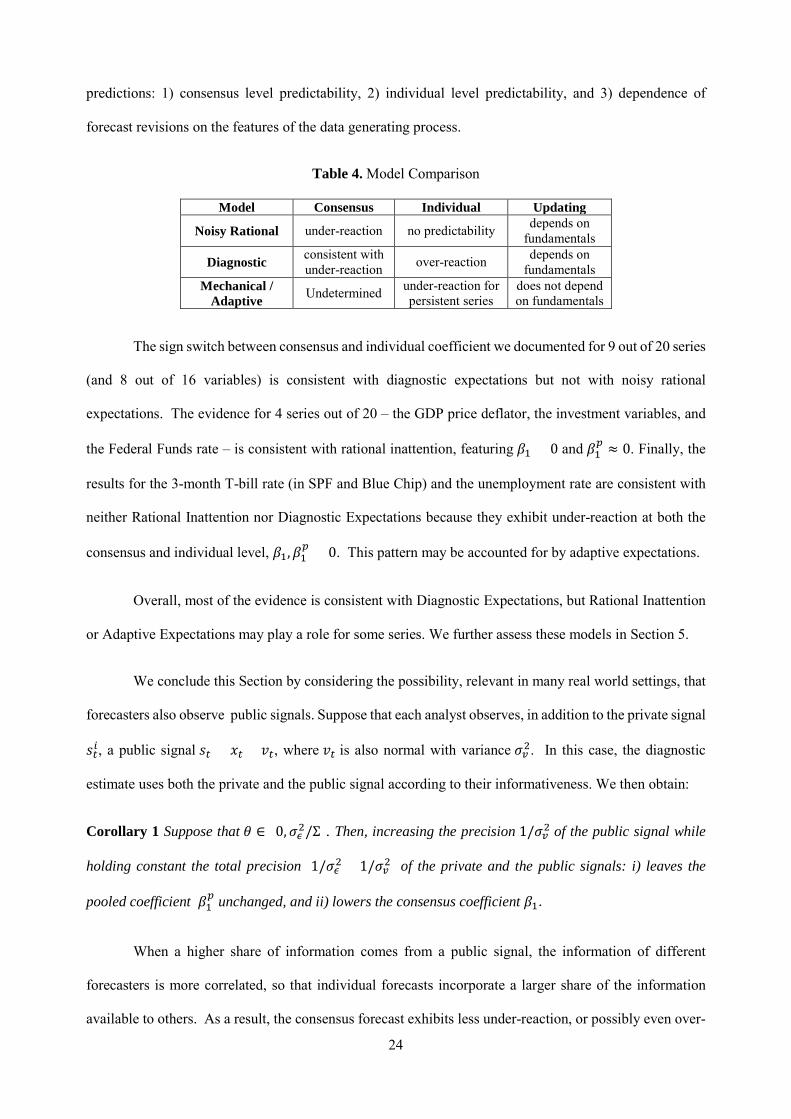
24

predictions: 1) consensus level predictability, 2) individual level predictability, and 3) dependence of

forecast revisions on the features of the data generating process.

Table 4. Model Comparison

Model Consensus Individual Updating

Noisy Rational under-reaction no predictability depends on fundamentals

Diagnostic consistent with under-reaction over-reaction depends on

fundamentals Mechanical /

Adaptive Undetermined under-reaction for persistent series

does not depend on fundamentals

The sign switch between consensus and individual coefficient we documented for 9 out of 20 series

(and 8 out of 16 variables) is consistent with diagnostic expectations but not with noisy rational

expectations. The evidence for 4 series out of 20 – the GDP price deflator, the investment variables, and

the Federal Funds rate – is consistent with rational inattention, featuring 𝛽𝛽1 > 0 and 𝛽𝛽1𝑝𝑝 ≈ 0. Finally, the

results for the 3-month T-bill rate (in SPF and Blue Chip) and the unemployment rate are consistent with

neither Rational Inattention nor Diagnostic Expectations because they exhibit under-reaction at both the

consensus and individual level, 𝛽𝛽1,𝛽𝛽1𝑝𝑝 > 0. This pattern may be accounted for by adaptive expectations.

Overall, most of the evidence is consistent with Diagnostic Expectations, but Rational Inattention

or Adaptive Expectations may play a role for some series. We further assess these models in Section 5.

We conclude this Section by considering the possibility, relevant in many real world settings, that

forecasters also observe public signals. Suppose that each analyst observes, in addition to the private signal

𝑠𝑠𝑡𝑡𝑖𝑖, a public signal 𝑠𝑠𝑡𝑡 = 𝑥𝑥𝑡𝑡 + 𝑐𝑐𝑡𝑡, where 𝑐𝑐𝑡𝑡 is also normal with variance 𝜎𝜎𝑣𝑣2. In this case, the diagnostic

estimate uses both the private and the public signal according to their informativeness. We then obtain:

Corollary 1 Suppose that 𝜃𝜃 ∈ (0,𝜎𝜎𝜖𝜖2/Σ). Then, increasing the precision 1/𝜎𝜎𝑣𝑣2 of the public signal while

holding constant the total precision (1/𝜎𝜎𝜖𝜖2 + 1/𝜎𝜎𝑣𝑣2) of the private and the public signals: i) leaves the

pooled coefficient 𝛽𝛽1𝑝𝑝 unchanged, and ii) lowers the consensus coefficient 𝛽𝛽1.

When a higher share of information comes from a public signal, the information of different

forecasters is more correlated, so that individual forecasts incorporate a larger share of the information

available to others. As a result, the consensus forecast exhibits less under-reaction, or possibly even over-

25

reaction. This may explain why in financial market variables such as interest rates we detect less consensus

under-reaction than in most other series: market prices act as public signals that correlate to a significant

extent the information sets of different forecasters.

The results in this section describe the features of over-reaction implied by diagnostic expectations.

It is useful to compare over-reaction in this specific setting to the concept of overconfidence, modeled as

overweighting of private signals relative to public signals (Daniel et al. 1998).15 Inflating the signal to

noise ratio of private information can cause over-reaction, by boosting the Kalman gain closer to its upper

bound of 1. In contrast, under diagnostic expectations, the Kalman gain is multiplied by (1 + 𝜃𝜃) and so

the reaction to information is not bounded by 1 (see Equation 8). In our estimation in Section 6, we find

clear evidence for the latter for several series. This difference has important implications for consensus

forecasts: Proposition 2 shows that consensus forecasts can over-react when the diagnostic Kalman gain

is large, which cannot happen under overconfidence. Moreover, Corollary 1 shows that there is more

consensus over-reaction when there is more public information, another result that cannot be obtained

from overconfidence, which predicts more under-reaction when more information is public.

5. Kernel of Truth

We first run a cross sectional test based on the persistence of the different series, which allows us

to compare Diagnostic Expectations with Adaptive Expectations. We then assess whether, for series that

feature hump-shaped dynamics, beliefs over-react both to short-term news and to longer-term reversals.

5.1 Persistence Tests

Under Noisy Rational and Diagnostic Expectations forecast revision at 𝑡𝑡 satisfies:

𝑥𝑥𝑡𝑡+ℎ|𝑡𝑡𝑖𝑖 − 𝑥𝑥𝑡𝑡+ℎ|𝑡𝑡−1

𝑖𝑖 = 𝜌𝜌�𝑥𝑥𝑡𝑡+ℎ−1|𝑡𝑡𝑖𝑖 − 𝑥𝑥𝑡𝑡+ℎ−1|𝑡𝑡−1

𝑖𝑖 �.

15 As mentioned in the Introduction, diagnostic expectations describe beliefs in a wide range of settings, both in the lab and in the field, including those where overconfidence can be ruled out (such as when all information is public, for example in experimental illustrations of base rate neglect or social stereotypes, BCGS 2016).

26

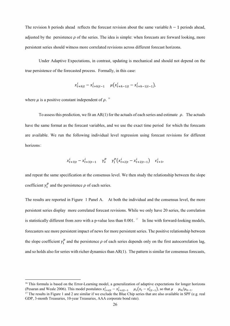
The revision h periods ahead reflects the forecast revision about the same variable ℎ − 1 periods ahead,

adjusted by the persistence 𝜌𝜌 of the series. The idea is simple: when forecasts are forward looking, more

persistent series should witness more correlated revisions across different forecast horizons.

Under Adaptive Expectations, in contrast, updating is mechanical and should not depend on the

true persistence of the forecasted process. Formally, in this case:

𝑥𝑥𝑡𝑡+ℎ|𝑡𝑡𝑖𝑖 − 𝑥𝑥𝑡𝑡+ℎ|𝑡𝑡−1

𝑖𝑖 = 𝜇𝜇�𝑥𝑥𝑡𝑡+ℎ−1|𝑡𝑡𝑖𝑖 − 𝑥𝑥𝑡𝑡+ℎ−1|𝑡𝑡−1

𝑖𝑖 �,

where 𝜇𝜇 is a positive constant independent of 𝜌𝜌.16

To assess this prediction, we fit an AR(1) for the actuals of each series and estimate 𝜌𝜌. The actuals

have the same format as the forecast variables, and we use the exact time period for which the forecasts

are available. We run the following individual level regression using forecast revisions for different

horizons:

𝑥𝑥𝑡𝑡+3|𝑡𝑡𝑖𝑖 − 𝑥𝑥𝑡𝑡+3|𝑡𝑡−1

𝑖𝑖 = 𝛾𝛾𝑜𝑜𝑝𝑝 + 𝛾𝛾1

𝑝𝑝�𝑥𝑥𝑡𝑡+2|𝑡𝑡𝑖𝑖 − 𝑥𝑥𝑡𝑡+2|𝑡𝑡−1

𝑖𝑖 � + 𝜖𝜖𝑡𝑡+3𝑖𝑖 ,

and repeat the same specification at the consensus level. We then study the relationship between the slope

coefficient 𝛾𝛾1𝑝𝑝 and the persistence 𝜌𝜌 of each series.

The results are reported in Figure 1 Panel A. At both the individual and the consensus level, the more

persistent series display more correlated forecast revisions. While we only have 20 series, the correlation

is statistically different from zero with a p-value less than 0.001.17 In line with forward-looking models,

forecasters see more persistent impact of news for more persistent series. The positive relationship between

the slope coefficient 𝛾𝛾1𝑝𝑝 and the persistence 𝜌𝜌 of each series depends only on the first autocorrelation lag,

and so holds also for series with richer dynamics than AR(1). The pattern is similar for consensus forecasts,

16 This formula is based on the Error-Learning model, a generalization of adaptive expectations for longer horizons (Pesaran and Weale 2006). This model postulates 𝑥𝑥𝑡𝑡+𝑠𝑠|𝑡𝑡

𝑖𝑖 − 𝑥𝑥𝑡𝑡+𝑠𝑠|𝑡𝑡−1𝑖𝑖 = 𝜇𝜇𝑠𝑠�𝑥𝑥𝑡𝑡 − 𝑥𝑥𝑡𝑡|𝑡𝑡−1

𝑖𝑖 �, so that 𝜇𝜇 = 𝜇𝜇ℎ/𝜇𝜇ℎ−1. 17 The results in Figure 1 and 2 are similar if we exclude the Blue Chip series that are also available in SPF (e.g. real GDP, 3-month Treasuries, 10-year Treasuries, AAA corporate bond rate).

27

shown in Figure 1 Panel B. This evidence is inconsistent with adaptive expectations, in which updating

does not depend on persistence, in which case the line in Figure 1 should be flat.

Figure 1. Properties of Forecast Revisions and Actuals

In Panel A, the y-axis is the coefficient 𝛾𝛾1𝑝𝑝from regression 𝑥𝑥𝑡𝑡+3|𝑡𝑡

𝑖𝑖 − 𝑥𝑥𝑡𝑡+3|𝑡𝑡−1𝑖𝑖 = 𝛾𝛾𝑜𝑜

𝑝𝑝 + 𝛾𝛾1𝑝𝑝�𝑥𝑥𝑡𝑡+2|𝑡𝑡

𝑖𝑖 − 𝑥𝑥𝑡𝑡+2|𝑡𝑡−1𝑖𝑖 � + 𝜖𝜖𝑡𝑡+3𝑖𝑖 .

The x-axis is the persistence measured from an AR(1) regression of the actuals corresponding to the forecasts. For each variable, the AR(1) regression uses the same time period as when the forecast data is available. In Panel B, the y-axis is the regression coefficient from the parallel specification using consensus forecasts.

Panel A. Individual Level Coefficients

Panel B. Consensus Coefficients

28

Another approach is to assess the correlation between the persistence of a series and the CG

coefficient of reaction to news. Diagnostic Expectations do not have clear predictions at the consensus

level: the coefficient (𝜎𝜎𝜖𝜖2 − 𝜃𝜃Σ)𝑔𝑔(𝜎𝜎𝜖𝜖2, Σ,𝜌𝜌,𝜃𝜃) in Equation (10) can be either decreasing or increasing in

persistence 𝜌𝜌, depending on the parameter values. On the other hand, Equation (11) says that the individual

CG coefficient should increase, i.e. get closer to zero, as 𝜌𝜌 increases. When the series is more persistent,

rational revisions become more volatile, which reduces the predictability of errors for a given level of

noise. Of course, under Noisy Rational Expectations individual coefficients should be zero, so they should

be uncorrelated with the persistence of fundamentals.

Figure 2 shows the correlation for the CG coefficient estimated from individual-level regressions.

We find that the CG coefficient rises with persistence, which lends additional support for diagnostic

expectations. The correlation is statistically different from zero with a p-value of 0.035.

Figure 2. CG Regression Coefficients and Persistence of Actual

Plots of individual level CG regression (forecast error on forecast revision) coefficients in the y-axis, against the persistence of the actual process in the x-axis.

29

5.2. Kernel of Truth in the Time Series

We now allow the forecasted series to be described by an AR(2) process. As shown by Fuster,

Laibson and Mendel (2010), several macroeconomic variables follow hump-shaped dynamics with short-

term momentum and longer-term reversals. Considering this possibility is relevant for two reasons. First,

under the kernel of truth, forecasters should exaggerate true features of the data generating process,

including the presence of long-term reversals. This also allows us to compare these approaches to the

model of Natural Expectations proposed by Fuster, Laibson and Mendel (2010), in which agents forecast

an AR(2) process “as if” it was AR(1) in changes.

5.2.1 Diagnostic Expectations with AR(2) Processes

Suppose that forecasters seek to forecast an AR(2) process:

𝑥𝑥𝑡𝑡+3 = 𝜌𝜌2𝑥𝑥𝑡𝑡+2 + 𝜌𝜌1𝑥𝑥𝑡𝑡+1 + 𝑢𝑢𝑡𝑡+3. (12)

If 𝜌𝜌2 > 0 and 𝜌𝜌1 < 0, the variable displays short-term momentum and long-term reversal. Each forecaster

now observes two signals, one about the current state 𝑠𝑠𝑡𝑡,𝑡𝑡𝑖𝑖 = 𝑥𝑥𝑡𝑡 + 𝜖𝜖𝑡𝑡𝑖𝑖 and another about the past state

𝑠𝑠𝑡𝑡−1,𝑡𝑡𝑖𝑖 = 𝑥𝑥𝑡𝑡−1 + 𝑐𝑐𝑡𝑡𝑖𝑖. The presence of two signals implies that the current forecast revisions for 𝑥𝑥𝑡𝑡+1 and

𝑥𝑥𝑡𝑡+2 are not perfectly collinear, which is necessary for out test.

The diagnostic forecasts about 𝑡𝑡 + 1 and 𝑡𝑡 + 2 overweigh each signal (this is proved in Appendix

A), so that forecast revisions are excessive. The diagnostic forecast of 𝑥𝑥𝑡𝑡+3 is then a linear combination

of the forecasts of 𝑥𝑥𝑡𝑡+2 and 𝑥𝑥𝑡𝑡+1 with weights given by the autoregressive parameters 𝜌𝜌1 and 𝜌𝜌2:

𝑥𝑥𝑡𝑡+3|𝑡𝑡𝑖𝑖,𝜃𝜃 = 𝜌𝜌2𝑥𝑥𝑡𝑡+2|𝑡𝑡

𝑖𝑖,𝜃𝜃 + 𝜌𝜌1𝑥𝑥𝑡𝑡+1|𝑡𝑡𝑖𝑖,𝜃𝜃 .

This formula suggests a way to test for overreaction, generalizing Equation (2) to AR(2). To do

so, simply predict forecast errors in the long term using forecast revisions about shorter term:

𝑥𝑥𝑡𝑡+3 − 𝑥𝑥𝑡𝑡+3|𝑡𝑡𝑖𝑖 = 𝛿𝛿0

𝑝𝑝 + 𝛿𝛿2𝑝𝑝𝐹𝐹𝑅𝑅𝑡𝑡,𝑡𝑡+2

𝑖𝑖 + 𝛿𝛿1𝑝𝑝𝐹𝐹𝑅𝑅𝑡𝑡,𝑡𝑡+1

𝑖𝑖 + 𝜖𝜖𝑡𝑡,𝑡𝑡+ℎ , (12)

where 𝐹𝐹𝑅𝑅𝑡𝑡,𝑡𝑡+1𝑖𝑖 and 𝐹𝐹𝑅𝑅𝑡𝑡,𝑡𝑡+2

𝑖𝑖 stand for the surveyed forecast revisions at for 𝑡𝑡 + 1 and 𝑡𝑡 + 2, respectively.

Under diagnostic expectations, estimates of (12) satisfy the following property.

30

Proposition 3. Under the Diagnostic Kalman filter, the estimated coefficients 𝛿𝛿1𝑝𝑝 and 𝛿𝛿2

𝑝𝑝 in Equation (12)

are proportional to the negative of the AR(2) coefficients:

𝛿𝛿1𝑝𝑝 ∝ −𝜌𝜌1𝜃𝜃, (13)

𝛿𝛿2𝑝𝑝 ∝ −𝜌𝜌2𝜃𝜃. (14)

Once again, under rational expectations (𝜃𝜃 = 0) individual forecast errors cannot be predicted

from any forecast revisions. Diagnostic expectations instead imply that the coefficients should be non-

zero, with flipped signs relative to the data generating process. This is due to the kernel of truth. Over-

reaction to short term news, 𝜌𝜌2 > 0, implies that upward forecast revisions about 𝑥𝑥𝑡𝑡+2 lead to exaggerated

optimism about 𝑥𝑥𝑡𝑡+3 and thus negative forecast errors. This yields 𝛿𝛿2𝑝𝑝 < 0. On the other hand, over-

reaction to long-term reversal, 𝜌𝜌1 < 0 , implies that upward forecast revisions about 𝑥𝑥𝑡𝑡+1 lead to

exaggerated pessimism about 𝑥𝑥𝑡𝑡+3 and thus positive forecast errors. This yields 𝛿𝛿1𝑝𝑝 > 0.18

Before moving to the data, we link this discussion to Natural Expectations, which have been

proposed to account for expectations errors in AR(2) settings. In this model, forecasts are based on an

AR(1) process in changes.19 This implies that Natural Expectations exaggerate the short run persistence of

the series and, similarly to Diagnostic Expectations, entail negative predictability of forecast errors at this

horizon. On the other hand, Natural Expectations also dampen long-term reversals, unlike our prediction

of over-reaction to long-term reversals (𝛿𝛿1𝑝𝑝 > 0 ). Thus, the two models predict overlapping but

distinguishable patterns of predictable forecast errors.

In the remainder of the section, we test the predictions of Proposition 3.

18 Proposition 3 also implies that the tests of Section 3 may be biased toward finding under-reaction when the AR(2) process has 𝜌𝜌2 > 0 and 𝜌𝜌1 < 0. Positive news at 𝑡𝑡 may then trigger an upward revision of the forecasts for both 𝑥𝑥𝑡𝑡+1 and 𝑥𝑥𝑡𝑡+2. The former creates excess pessimism, the latter excess optimism. If the first effect is strong, the test of Section 3 may detect excess pessimism after good news, giving a false impression of under-reaction. 19 Formally, forecasters use the rule (𝑥𝑥𝑡𝑡+1 − 𝑥𝑥𝑡𝑡) = 𝜑𝜑(𝑥𝑥𝑡𝑡 − 𝑥𝑥𝑡𝑡−1) + 𝑐𝑐𝑡𝑡+1 with fitted coefficient 𝜑𝜑 = (𝜌𝜌2 −𝜌𝜌1 − 1)/2. For a stationary AR(2) process (i.e. if 𝜌𝜌2 − 𝜌𝜌1 < 1 , 𝜌𝜌1 + 𝜌𝜌2 < 1 and |𝜌𝜌1| < 1 ) this implies that forecasters exaggerate short term momentum and dampen long term reversals. This model cannot be directly estimated using Equation (12) because it implies that the two forecast revisions are perfectly collinear.

31

5.2.2 AR(1) vs AR(2) Dynamics

As a first step, we assess which of our 16 variables is more accurately described by AR(2) rather

than AR(1). We do not aim to find the unconstrained optimal ARMA(𝑘𝑘, 𝑞𝑞) specification, which is well

known to be difficult. We only wish to capture the simplest longer lags and see whether expectations react

to them as predicted by the model. We fit a quarterly AR(2) process for our 20 series. Figure 4 below

plots the estimates for 𝜌𝜌1 and 𝜌𝜌2.20 As before, the actuals have the same format as the forecast variables,

and for each series the regression covers the time period when the forecast data are available.

The signs of coefficients point to a positive momentum at short horizons (𝜌𝜌2 > 0) for all series,

and to long-run reversals (𝜌𝜌1 < 0) for most series, the remaining ones having 𝜌𝜌1 approximately zero.21 To

assess which dynamics better describe the series, we compare the AR(2) estimates to the AR(1) estimates

from Section 5.1. Table 6 shows the Bayesian Information Criterion (BIC) score associated with each fit.

For the majority of series, AR(2) is favored over AR(1). The tests favor AR(1) dynamics only for

real consumption (SPF) and the BAA bond rate (BC), while for the 10-year Treasury rate series the tests

are inconclusive.22 In sum, hump shaped dynamics are a key feature of several series.

20 Just like for the case of AR(1), for growth variables we run quarterly AR(2) regressions of growth from 𝑡𝑡 − 1 to 𝑡𝑡 + 3. For variables in levels, we run quarterly regressions in levels. We run separate regressions for the variables that occur both in SPF and BC, because they cover slightly different time periods. 21 We check whether multicollinearity may affect our results in this Section, given that forecasts revisions at different horizons are often highly correlated. The standard issue with multicollinearity is the coefficients are imprecisely estimated, which we do not find to be the case. We also perform simulations to verify that the correlation among the right hand side variables by itself does not mechanically lead to the patterns we observe. 22 The Akaike Information Criterion (AIC) yields similar results, except that it positively identifies the TN10Y (SPF) series as AR(2). To interpret the IC scores, recall that lower scores represent a better fit. The likelihood ratio Pr(𝐴𝐴𝐴𝐴2)

Pr(𝐴𝐴𝐴𝐴1)

is estimated as 𝑒𝑒𝑥𝑥𝑝𝑝 �− 𝐵𝐵𝐼𝐼𝐵𝐵𝐴𝐴𝐴𝐴2−𝐵𝐵𝐼𝐼𝐵𝐵𝐴𝐴𝐴𝐴12

�, so that ∆𝐵𝐵𝐼𝐼𝐵𝐵2−1 = −2 means the AR(2) model is 2.7 times more likely than the AR(1) model.

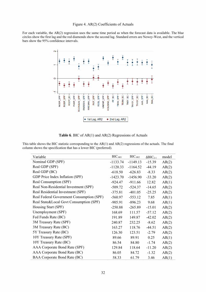
32

Figure 4. AR(2) Coefficients of Actuals

For each variable, the AR(2) regression uses the same time period as when the forecast data is available. The blue circles show the first lag and the red diamonds show the second lag. Standard errors are Newey-West, and the vertical bars show the 95% confidence intervals.

Table 6. BIC of AR(1) and AR(2) Regressions of Actuals

This table shows the BIC statistic corresponding to the AR(1) and AR(2) regressions of the actuals. The final column shows the specification that has a lower BIC (preferred).

Variable BICAR1 BICAR2 ∆BIC2-1 model Nominal GDP (SPF) -1133.74 -1149.13 -15.39 AR(2) Real GDP (SPF) -1120.33 -1164.52 -44.19 AR(2) Real GDP (BC) -618.50 -626.83 -8.33 AR(2) GDP Price Index Inflation (SPF) -1423.70 -1456.90 -33.20 AR(2) Real Consumption (SPF) -924.47 -911.66 12.82 AR(1) Real Non-Residential Investment (SPF) -509.72 -524.37 -14.65 AR(2) Real Residential Investment (SPF) -375.81 -401.05 -25.25 AR(2) Real Federal Government Consumption (SPF) -560.97 -553.12 7.85 AR(1) Real State&Local Govt Consumption (SPF) -905.91 -896.23 9.68 AR(1) Housing Start (SPF) -250.88 -265.89 -15.01 AR(2) Unemployment (SPF) 168.69 111.57 -57.12 AR(2) Fed Funds Rate (BC) 191.89 149.87 -42.02 AR(2) 3M Treasury Rate (SPF) 240.87 232.25 -8.62 AR(2) 3M Treasury Rate (BC) 163.27 118.76 -44.51 AR(2) 5Y Treasury Rate (BC) 126.30 123.51 -2.79 AR(2) 10Y Treasury Rate (SPF) 89.66 89.91 0.25 AR(1) 10Y Treasury Rate (BC) 86.54 84.80 -1.74 AR(2) AAA Corporate Bond Rate (SPF) 129.84 118.64 -11.20 AR(2) AAA Corporate Bond Rate (BC) 86.05 84.72 -1.32 AR(2) BAA Corporate Bond Rate (BC) 58.33 61.79 3.46 AR(1)

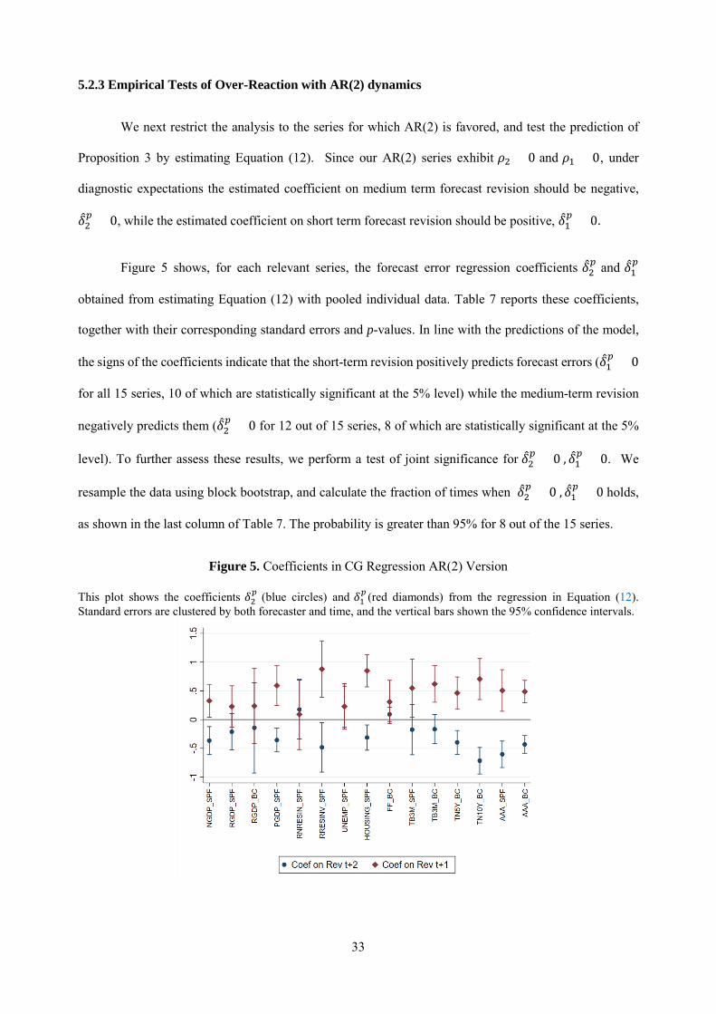
33

5.2.3 Empirical Tests of Over-Reaction with AR(2) dynamics

We next restrict the analysis to the series for which AR(2) is favored, and test the prediction of

Proposition 3 by estimating Equation (12). Since our AR(2) series exhibit 𝜌𝜌2 > 0 and 𝜌𝜌1 < 0, under

diagnostic expectations the estimated coefficient on medium term forecast revision should be negative,

𝛿𝛿2𝑝𝑝 < 0, while the estimated coefficient on short term forecast revision should be positive, 𝛿𝛿1

𝑝𝑝 > 0.

Figure 5 shows, for each relevant series, the forecast error regression coefficients 𝛿𝛿2𝑝𝑝 and 𝛿𝛿1

𝑝𝑝

obtained from estimating Equation (12) with pooled individual data. Table 7 reports these coefficients,

together with their corresponding standard errors and p-values. In line with the predictions of the model,

the signs of the coefficients indicate that the short-term revision positively predicts forecast errors (𝛿𝛿1𝑝𝑝 > 0

for all 15 series, 10 of which are statistically significant at the 5% level) while the medium-term revision

negatively predicts them (𝛿𝛿2𝑝𝑝 < 0 for 12 out of 15 series, 8 of which are statistically significant at the 5%

level). To further assess these results, we perform a test of joint significance for 𝛿𝛿2𝑝𝑝 < 0 , 𝛿𝛿1

𝑝𝑝 > 0. We

resample the data using block bootstrap, and calculate the fraction of times when 𝛿𝛿2𝑝𝑝 < 0 , 𝛿𝛿1

𝑝𝑝 > 0 holds,

as shown in the last column of Table 7. The probability is greater than 95% for 8 out of the 15 series.

Figure 5. Coefficients in CG Regression AR(2) Version

This plot shows the coefficients 𝛿𝛿2𝑝𝑝 (blue circles) and 𝛿𝛿1

𝑝𝑝 (red diamonds) from the regression in Equation (12). Standard errors are clustered by both forecaster and time, and the vertical bars shown the 95% confidence intervals.

34

Table 7. Coefficients in CG Regression AR(2) Version Coefficients 𝛿𝛿2

𝑝𝑝and 𝛿𝛿1𝑝𝑝 from the regression in Equation (12), together with the corresponding standard errors and p-

values. The final column resamples the data using block bootstrap and shows the probability of 𝛿𝛿2𝑝𝑝 < 0 and 𝛿𝛿1

𝑝𝑝 > 0.

Variable 𝛿𝛿2𝑝𝑝 s.e. p-val 𝛿𝛿1

𝑝𝑝 s.e. p-val Prob 𝛿𝛿2𝑝𝑝 < 0

& 𝛿𝛿1𝑝𝑝 > 0

Nominal GDP (SPF) -0.37 0.12 0.00 0.33 0.15 0.03 0.99 Real GDP (SPF) -0.21 0.16 0.19 0.23 0.18 0.22 0.86 Real GDP (BC) -0.14 0.40 0.72 0.24 0.33 0.48 0.78 GDP Price Index Inflation (SPF) -0.36 0.11 0.00 0.59 0.18 0.00 0.99 Real Non-Residential Investment (SPF) 0.18 0.26 0.50 0.09 0.31 0.77 0.11 Real Residential Investment (SPF) -0.48 0.22 0.03 0.88 0.25 0.00 1.00 Housing Start (SPF) -0.31 0.11 0.01 0.85 0.14 0.00 1.00 Unemployment (SPF) 0.23 0.18 0.22 0.23 0.20 0.26 0.03 Fed Funds Rate (BC) 0.09 0.06 0.15 0.31 0.19 0.11 0.40 3M Treasury Rate (SPF) -0.17 0.22 0.43 0.55 0.26 0.03 0.85 3M Treasury Rate (BC) -0.17 0.13 0.20 0.62 0.16 0.00 0.92 5Y Treasury Rate (BC) -0.40 0.11 0.00 0.46 0.14 0.00 1.00 10Y Treasury Rate (BC) -0.72 0.12 0.00 0.71 0.18 0.00 1.00 AAA Corporate Bond Rate (SPF) -0.60 0.12 0.00 0.51 0.18 0.01 1.00 AAA Corporate Bond Rate (BC) -0.43 0.08 0.00 0.49 0.10 0.00 1.00

These results are consistent with kernel of truth but are harder to reconcile with Natural

Expectations, where forecasters neglect longer lags (in the current setting, this means fitting an AR(1)

model even for AR(2) series).23 Overall, then, the AR(2) analysis confirms and perhaps strengthens the

evidence for over-reaction in the data. Four of the seven series (PGDP_SPF, RRESINV_SPF, TN5Y_BC

and TN10Y_BC) for which individual level forecast errors seemed unpredictable (Table 3), and thus

consistent with Noisy Rational Expectations, show evidence of over-reaction in the AR(2) setting. In

addition, the two series that seemed to display under-reaction at the individual level, unemployment and

the 3-months T Bill rate, now show evidence of over-reaction to long-term reversals (𝛿𝛿1𝑝𝑝 > 0), albeit not

significantly. In all these cases, it is possible that over-reaction to long term reversals moved the individual

level coefficient in Table 4 close to zero or above, giving the false impression of rationality or under-

reaction. Only for the variable RGDP_SPF, which displayed significant over-reaction under the AR(1)

specification loses its significance at conventional level in the AR(2) case.

23 Beshears et al. (2013) report results from a laboratory experiment in which subjects recognize reversals occurring within ten periods, but not in fifty periods. In our data reversals are fast, which is consistent with their findings.

35

6. Model Estimation

We next use the simulated method of moments to quantify 𝜃𝜃 and assess the performance of our

model. In the baseline quantification, we assume that shocks are normal and that the macro series follow

the better-fitting process among AR(1) or AR(2). We then present a sensitivity analysis. We first estimate

𝜃𝜃 under the assumption that all series follow an AR(1). The results are similar, which is reassuring given

the well known difficulty of finding the proper AR specification. We next allow for fundamental shocks to

be drawn from fat tailed distributions. Using the particle filter, we find that our results again remain stable.

Finally, we estimate an overconfidence model, and show that diagnostic expectations better fit of the data

quantitatively. Appendix E presents supporting material for these exercises.

The estimation exercises share the following general structure. First, we assume forecasters

describe each series 𝑘𝑘 using the vector of estimated fundamental parameters ((𝜌𝜌1,𝑘𝑘,𝜎𝜎𝑢𝑢,𝑘𝑘) for the AR(1)

specifications and (𝜌𝜌1,𝑘𝑘,𝜌𝜌2,𝑘𝑘 ,𝜎𝜎𝑢𝑢,𝑘𝑘) for the AR(2) specifications). By separating the estimation of

fundamental and expectations parameters, we minimize the degrees of freedom in fitting expectations data.

Second, given these parameter values we use the simulated method of moments to estimate, for each

expectations series, the series-specific measurement noise 𝜎𝜎𝜀𝜀,𝑘𝑘 and the diagnostic parameter 𝜃𝜃𝑘𝑘 . We

initially take (𝜃𝜃𝑘𝑘,𝜎𝜎𝜀𝜀,𝑘𝑘) to be common to all forecasters, but also estimate them at the forecaster level.

We estimate 𝜎𝜎𝜀𝜀,𝑘𝑘 and 𝜃𝜃𝑘𝑘 by matching two moments of the expectations data: the variance of the

forecast errors, 𝜎𝜎𝐹𝐹𝐹𝐹,𝑘𝑘2 = 𝑐𝑐𝑣𝑣𝑣𝑣𝑖𝑖,𝑡𝑡�𝐹𝐹𝐹𝐹𝑘𝑘,𝑡𝑡

𝑖𝑖 � , and the variance of forecast revisions, 𝜎𝜎𝐹𝐹𝐴𝐴,𝑘𝑘2 = 𝑐𝑐𝑣𝑣𝑣𝑣𝑖𝑖,𝑡𝑡�𝐹𝐹𝑅𝑅𝑘𝑘,𝑡𝑡

𝑖𝑖 � ,

computed across time and forecasters. We choose these moments because they can be measured directly

from the data with reasonable precision and they are linked to the parameters of interest.24 By the law of

total variance, the variance of forecast errors 𝜎𝜎𝐹𝐹𝐹𝐹,𝑘𝑘2 is the sum of the: i) average cross sectional variance of

errors, and the ii) over time variance of consensus errors. The first term is informative about measurement

noise 𝜎𝜎𝜀𝜀,𝑘𝑘, without which any cross sectional variance would be zero. The second term is informative about

the over-reaction parameter 𝜃𝜃𝑘𝑘. A similar logic holds with respect to the total variance of forecast revisions.

24 In contrast, matching average forecast errors and revisions would not be informative about 𝜎𝜎𝜀𝜀,𝑘𝑘 and 𝜃𝜃𝑘𝑘, as these sample moments are close to zero in our data (consistently with diagnostic but also rational expectations). Importantly, we do not use the CG coefficients in the estimation because we later use these moments to assess model performance.

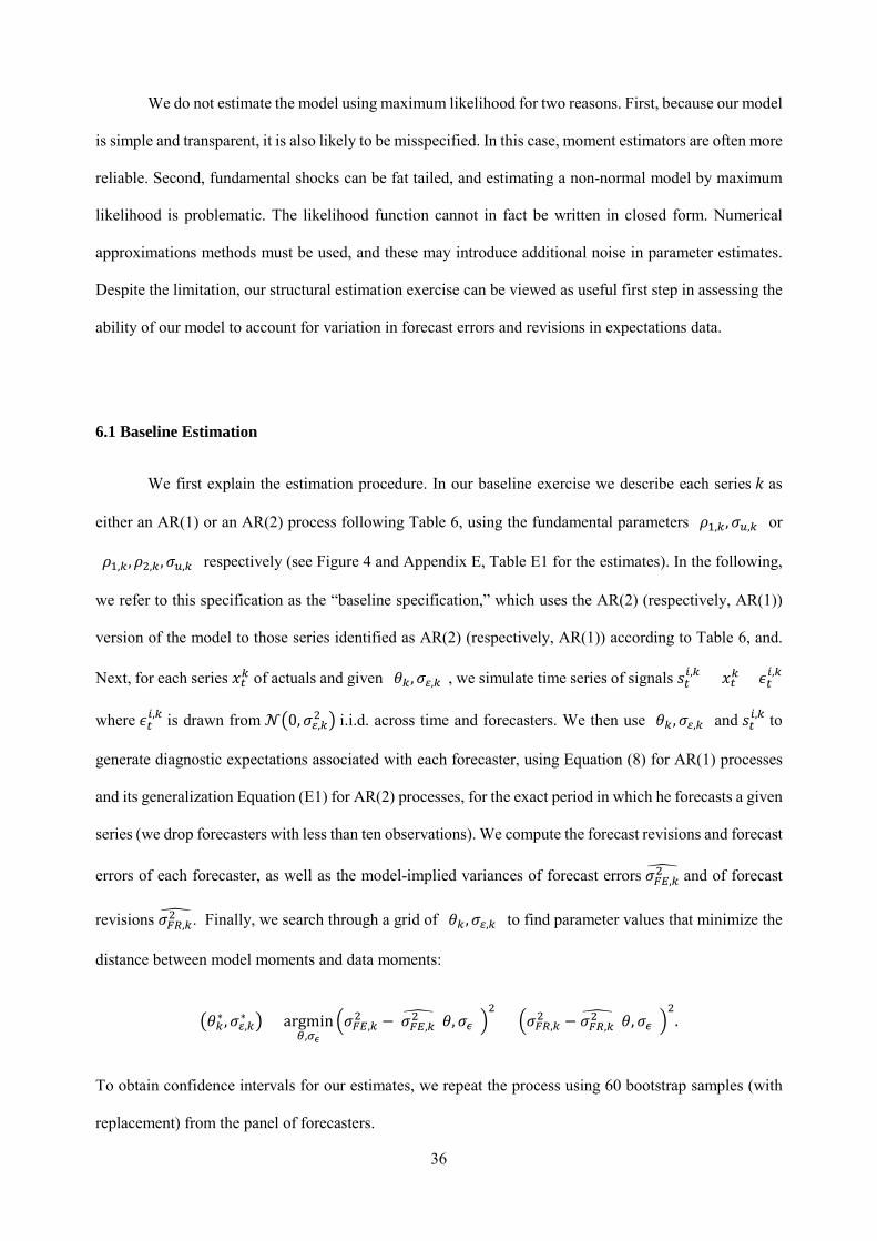
36

We do not estimate the model using maximum likelihood for two reasons. First, because our model

is simple and transparent, it is also likely to be misspecified. In this case, moment estimators are often more

reliable. Second, fundamental shocks can be fat tailed, and estimating a non-normal model by maximum

likelihood is problematic. The likelihood function cannot in fact be written in closed form. Numerical

approximations methods must be used, and these may introduce additional noise in parameter estimates.

Despite the limitation, our structural estimation exercise can be viewed as useful first step in assessing the

ability of our model to account for variation in forecast errors and revisions in expectations data.

6.1 Baseline Estimation

We first explain the estimation procedure. In our baseline exercise we describe each series 𝑘𝑘 as

either an AR(1) or an AR(2) process following Table 6, using the fundamental parameters (𝜌𝜌1,𝑘𝑘,𝜎𝜎𝑢𝑢,𝑘𝑘) or

(𝜌𝜌1,𝑘𝑘,𝜌𝜌2,𝑘𝑘,𝜎𝜎𝑢𝑢,𝑘𝑘) respectively (see Figure 4 and Appendix E, Table E1 for the estimates). In the following,

we refer to this specification as the “baseline specification,” which uses the AR(2) (respectively, AR(1))

version of the model to those series identified as AR(2) (respectively, AR(1)) according to Table 6, and.

Next, for each series 𝑥𝑥𝑡𝑡𝑘𝑘 of actuals and given (𝜃𝜃𝑘𝑘,𝜎𝜎𝜀𝜀,𝑘𝑘), we simulate time series of signals 𝑠𝑠𝑡𝑡𝑖𝑖,𝑘𝑘 = 𝑥𝑥𝑡𝑡𝑘𝑘 + 𝜖𝜖𝑡𝑡

𝑖𝑖,𝑘𝑘

where 𝜖𝜖𝑡𝑡𝑖𝑖,𝑘𝑘 is drawn from 𝒩𝒩�0,𝜎𝜎𝜀𝜀,𝑘𝑘

2 � i.i.d. across time and forecasters. We then use (𝜃𝜃𝑘𝑘 ,𝜎𝜎𝜀𝜀,𝑘𝑘) and 𝑠𝑠𝑡𝑡𝑖𝑖,𝑘𝑘 to

generate diagnostic expectations associated with each forecaster, using Equation (8) for AR(1) processes

and its generalization Equation (E1) for AR(2) processes, for the exact period in which he forecasts a given

series (we drop forecasters with less than ten observations). We compute the forecast revisions and forecast

errors of each forecaster, as well as the model-implied variances of forecast errors 𝜎𝜎𝐹𝐹𝐹𝐹,𝑘𝑘2� and of forecast

revisions 𝜎𝜎𝐹𝐹𝐴𝐴,𝑘𝑘2� . Finally, we search through a grid of (𝜃𝜃𝑘𝑘 ,𝜎𝜎𝜀𝜀,𝑘𝑘) to find parameter values that minimize the

distance between model moments and data moments:

�𝜃𝜃𝑘𝑘∗ ,𝜎𝜎𝜀𝜀,𝑘𝑘∗ � = argmin

(𝜃𝜃,𝜎𝜎𝜖𝜖)�𝜎𝜎𝐹𝐹𝐹𝐹,𝑘𝑘

2 − 𝜎𝜎𝐹𝐹𝐹𝐹,𝑘𝑘2� (𝜃𝜃,𝜎𝜎𝜖𝜖)�

2+ �𝜎𝜎𝐹𝐹𝐴𝐴,𝑘𝑘

2 − 𝜎𝜎𝐹𝐹𝐴𝐴,𝑘𝑘2� (𝜃𝜃,𝜎𝜎𝜖𝜖)�

2.

To obtain confidence intervals for our estimates, we repeat the process using 60 bootstrap samples (with

replacement) from the panel of forecasters.

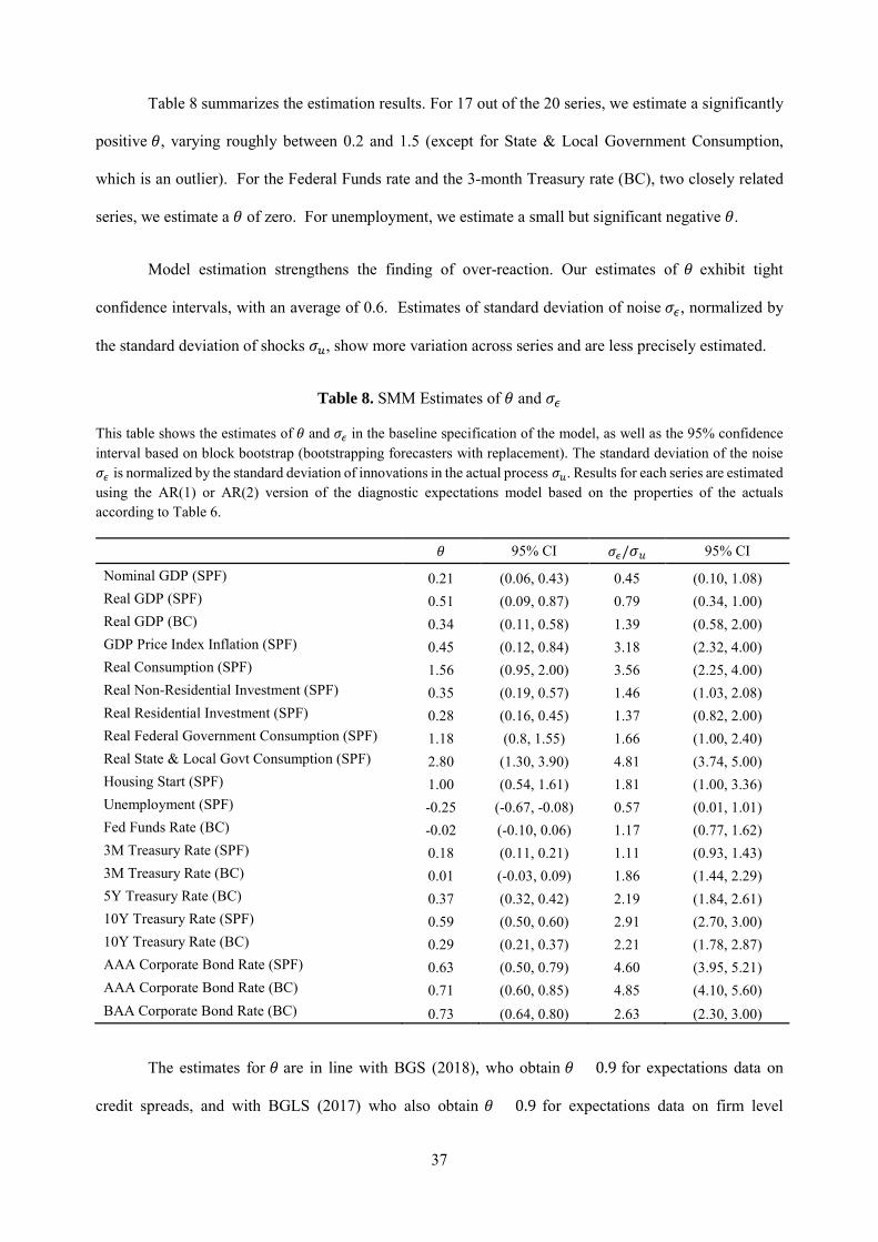
37

Table 8 summarizes the estimation results. For 17 out of the 20 series, we estimate a significantly

positive 𝜃𝜃, varying roughly between 0.2 and 1.5 (except for State & Local Government Consumption,

which is an outlier). For the Federal Funds rate and the 3-month Treasury rate (BC), two closely related

series, we estimate a 𝜃𝜃 of zero. For unemployment, we estimate a small but significant negative 𝜃𝜃.

Model estimation strengthens the finding of over-reaction. Our estimates of 𝜃𝜃 exhibit tight

confidence intervals, with an average of 0.6. Estimates of standard deviation of noise 𝜎𝜎𝜖𝜖, normalized by

the standard deviation of shocks 𝜎𝜎𝑢𝑢, show more variation across series and are less precisely estimated.

Table 8. SMM Estimates of 𝜃𝜃 and 𝜎𝜎𝜖𝜖 This table shows the estimates of 𝜃𝜃 and 𝜎𝜎𝜖𝜖 in the baseline specification of the model, as well as the 95% confidence interval based on block bootstrap (bootstrapping forecasters with replacement). The standard deviation of the noise 𝜎𝜎𝜖𝜖 is normalized by the standard deviation of innovations in the actual process 𝜎𝜎𝑢𝑢. Results for each series are estimated using the AR(1) or AR(2) version of the diagnostic expectations model based on the properties of the actuals according to Table 6.

𝜃𝜃 95% CI 𝜎𝜎𝜖𝜖/𝜎𝜎𝑢𝑢 95% CI

Nominal GDP (SPF) 0.21 (0.06, 0.43) 0.45 (0.10, 1.08) Real GDP (SPF) 0.51 (0.09, 0.87) 0.79 (0.34, 1.00) Real GDP (BC) 0.34 (0.11, 0.58) 1.39 (0.58, 2.00) GDP Price Index Inflation (SPF) 0.45 (0.12, 0.84) 3.18 (2.32, 4.00) Real Consumption (SPF) 1.56 (0.95, 2.00) 3.56 (2.25, 4.00) Real Non-Residential Investment (SPF) 0.35 (0.19, 0.57) 1.46 (1.03, 2.08) Real Residential Investment (SPF) 0.28 (0.16, 0.45) 1.37 (0.82, 2.00) Real Federal Government Consumption (SPF) 1.18 (0.8, 1.55) 1.66 (1.00, 2.40) Real State & Local Govt Consumption (SPF) 2.80 (1.30, 3.90) 4.81 (3.74, 5.00) Housing Start (SPF) 1.00 (0.54, 1.61) 1.81 (1.00, 3.36) Unemployment (SPF) -0.25 (-0.67, -0.08) 0.57 (0.01, 1.01) Fed Funds Rate (BC) -0.02 (-0.10, 0.06) 1.17 (0.77, 1.62) 3M Treasury Rate (SPF) 0.18 (0.11, 0.21) 1.11 (0.93, 1.43) 3M Treasury Rate (BC) 0.01 (-0.03, 0.09) 1.86 (1.44, 2.29) 5Y Treasury Rate (BC) 0.37 (0.32, 0.42) 2.19 (1.84, 2.61) 10Y Treasury Rate (SPF) 0.59 (0.50, 0.60) 2.91 (2.70, 3.00) 10Y Treasury Rate (BC) 0.29 (0.21, 0.37) 2.21 (1.78, 2.87) AAA Corporate Bond Rate (SPF) 0.63 (0.50, 0.79) 4.60 (3.95, 5.21) AAA Corporate Bond Rate (BC) 0.71 (0.60, 0.85) 4.85 (4.10, 5.60) BAA Corporate Bond Rate (BC) 0.73 (0.64, 0.80) 2.63 (2.30, 3.00)

The estimates for 𝜃𝜃 are in line with BGS (2018), who obtain 𝜃𝜃 = 0.9 for expectations data on

credit spreads, and with BGLS (2017) who also obtain 𝜃𝜃 = 0.9 for expectations data on firm level

38

earnings’ growth. In the current exercise the average estimate is a bit lower, but this may be due to the fact

that here we allow for AR(2) specifications (if we assume an AR(1) structure for all series, we find an

average 𝜃𝜃 of 0.81, see Section 6.3). To have a sense of the magnitude, a 𝜃𝜃 ≈ 1 means that forecasters’

reaction to news is roughly twice as large as the rational expectations benchmark. In BGLS (2017), we

find that this magnitude of 𝜃𝜃 can account for the observed 12% annual return spread between stocks

analysts are pessimistic about and stocks they are optimistic about. This suggests that this magnitude of

distortions can have sizable economic consequences.

6.2 Model Performance

We first assess the ability of the model to match the target moments. Across different series k, the

average absolute log difference between the variance of forecast errors in the data (𝜎𝜎𝐹𝐹𝐹𝐹,𝑘𝑘2 ) and that in the

simulated model (𝜎𝜎𝐹𝐹𝐹𝐹,𝑘𝑘2� (𝜃𝜃,𝜎𝜎𝜖𝜖)) is 0.022, with a minimum of 0.001 for the Fed Funds Rate and a maximum

of 0.207 for Real State and Local Government Consumption. Likewise, the variance of forecast revisions

in the data (𝜎𝜎𝐹𝐹𝐹𝐹,𝑘𝑘2 ) and that in the simulated model (𝜎𝜎𝐹𝐹𝐹𝐹,𝑘𝑘

2� (𝜃𝜃,𝜎𝜎𝜖𝜖)) is 0.028, with a minimum of 0.002 for

Housing Starts and a maximum of 0.188 for Unemployment Rate (see Appendix E, Table E2).

Second, we assess the ability of the model to match the Coibion-Gorodnichenko coefficients, at

the individual and consensus levels. We calculate the CG coefficients in the model using the estimated (𝜃𝜃,

𝜎𝜎𝜖𝜖) for each series, together with the actual process and its parameters, to generate model-based forecasts

associated with each forecaster and each time period where the forecaster is available; we then run CG

regressions using these model-based forecasts, and compare the results with CG regressions using survey

data. Figure 6 shows the individual CG coefficients from the estimated model and those from the survey

data. The correlation between the two sets of coefficients is high, about 0.83 (p-value of 0.00).

Figure 6. Individual CG Coefficients using Estimated 𝜃𝜃 and 𝜎𝜎𝜖𝜖

The figure plots individual CG coefficients in the baseline specification of the model (with estimated 𝜃𝜃 and 𝜎𝜎𝜖𝜖) in the y-axis, and CG coefficients in the survey data in the x-axis. Results for each series are estimated using the AR(1) or AR(2) version of the diagnostic expectations model based on the properties of the actuals according to Table 6.

39

For consensus CG coefficients, we also find a positive correlation between estimates from the

model and in the survey data, but the correlation is lower than in the individual case (0.30 vs 0.83, see

Appendix E Figure E1). The lower correlation reflects the fact that, unlike individual level coefficients,

consensus coefficients are highly dependent on the magnitude of measurement noise 𝜎𝜎𝜖𝜖,𝑘𝑘, which is less

precisely estimated as shown in Table 8.

6.3 Sensitivity Analysis and Overconfidence

We next assess the robustness of our results to alternative assumptions. We complement our

baseline specification above with two other specifications: we first restrict all series to follow an AR(1)

process, keeping the assumption of normal shocks; we then allow the fundamental shocks to be non-

normal, as macro series are known to have fat tails. Table E3 reports the estimated target moments, Table

E4 reports the 𝜃𝜃𝑘𝑘 estimates, and Table E5 assesses model performance in terms of reproducing individual

and consensus CG coefficients.

We find a very high correlation between the distortions 𝜃𝜃𝑘𝑘 estimated under the different

specifications, between 91% and 96%, and the average estimates for 𝜃𝜃 in the alternative specifications are

also very similar (0.6 in the baseline specification, 0.81 for AR(1) and 0.74 for AR(1) with fat tails and

particle filtering, see Table E4 for details). Our baseline estimates are robust to these alternative

specifications. In terms of model performance, the baseline specification (which allows for AR(2)) seems

to do a better job than the other ones. It achieves a lower value of the loss function (half as large as the next

40

best performer for the median series, based on moments shown in Table E2 and E3), and it explains a larger

share of variation in individual CG coefficients (see Table E5, panel A).

We also assess the ability of the model to capture observed heterogeneity in distortions across

different analysts. To do so, we estimate distortion and noise coefficients (𝜃𝜃𝑘𝑘𝑖𝑖 ,𝜎𝜎𝜖𝜖,𝑘𝑘𝑖𝑖 ) analyst by analyst.

Table E6 in Appendix E reports the median estimate of 𝜃𝜃𝑘𝑘𝑖𝑖 and 𝜎𝜎𝜖𝜖,𝑘𝑘𝑖𝑖 across forecasters for each series, which

confirms our previous results. The estimated 𝜃𝜃𝑘𝑘𝑖𝑖 are also generally positively correlated across series: Table

E7 shows that individuals who over-react more in forecasting certain series also tend to over-react more in

forecasting other series.25

Finally, we compare the performance of the diagnostic expectations model with the performance

of a model of overconfidence in which analysts perceive their noisy signals to be more informative than in

reality. To this end, we repeat the previous simulation procedures, but estimate parameters (𝛼𝛼𝑘𝑘 ,𝜎𝜎𝜖𝜖,𝑘𝑘),

where 𝜎𝜎𝜖𝜖,𝑘𝑘 is the actual volatility of the noise but forecasters perceive it to be 𝛼𝛼𝑘𝑘𝜎𝜎𝜖𝜖,𝑘𝑘 (see Appendix E.3).

In other words, 𝛼𝛼𝑘𝑘 < 1 captures the potential under-estimation of noise, which would inflate the Kalman

gain. To facilitate comparison, we focus on AR(1) fundamentals, for which both overconfidence and

diagnostic expectations can be collapsed into a single Kalman gain. Table E8 shows that the diagnostic

expectations model performs generally better than overconfidence. For 14 out of 20 series, it achieves a

smaller loss than the overconfidence model, and its loss is about a half of the latter’s loss for the median

series. This is mainly due to the fact that the overconfidence model bounds the extent of over-reaction by

forcing the Kalman gain to be at most one. The diagnostic Kalman gain is instead allowed to exceed one,

which is supported by the data for seven series, see Figure E2.

Overall, our structural estimation exercise yields three results. First, diagnostic distortions in

professional forecasters’ expectations are sizable and in the ballpark of previous estimates obtained in

different contexts. Representativeness is thus a promising candidate for a robust psychological distortion

in expectation formation. Second, the estimated distortions are quite robust to alternative assumptions.

Third, the diagnostic expectation model does a good job at capturing variation in the data.

25 Here we take heterogeneity of (𝜃𝜃𝑘𝑘𝑖𝑖 ,𝜎𝜎𝜖𝜖,𝑘𝑘

𝑖𝑖 ) as given, but it would be interesting in future work to explore its sources.

41

7. Conclusion

Using data from both the Blue Chip Survey and the Survey of Professional Forecasters, we have

investigated how professional forecasters react to information using the methodology of Coibion and

Gorodnichenko (2015). We have found that while under-reaction is the norm for the consensus forecast,

as previously shown by CG (2015), for individual forecasters the norm is over-reaction to information, in

the sense of forecast errors being (negatively) predictable from forecast revisions. We showed that

individual-level overreaction is robust to a wide range of possible confounds. We then applied a

psychologically founded model of belief formation, diagnostic expectations, to these data. We showed

that diagnostic expectations generate over-reaction in individual forecasts, but if different forecasters see

different information and/or use different models, the consensus forecast may exhibit under-reaction. The

model thus reconciles these seemingly opposite patterns in the data.

The kernel of truth property of diagnostic expectations yields several additional predictions as to

when we would see over-reaction in forecasts, and by how much, as a function of the series’ underlying

dynamics. These predictions are supported in the data, consistent with forecasters being forward looking

and their judgment distorted by representativeness. Thus, individual forecasts are better described by

diagnostic expectations than by mechanical models of extrapolation, such as adaptive expectations, which

have been criticized by Lucas (1976) precisely on the grounds that people are assumed to be entirely

backward looking. In fact, diagnostic expectations can serve as a micro-foundation of extrapolation, and

the latter may reflect the former at a crude level.

Our approach enables us to document and reconcile distinctive features of expectations data. At

the most basic level, it reconciles individual and consensus forecast patterns. Perhaps more subtly,

diagnostic expectations when extended to the AR(2) context enable us to model expectations for hump

shaped series. In this setting, diagnostic expectations capture some features of Natural Expectations (Fuster

et al. 2010), such as exaggeration of short term persistence, but also yield over-reaction to long term

reversal, which seems to be a feature of the data. Finally, unlike overconfidence, diagnostic expectations

can generate effective Kalman gains above 1, which also seem to describe several series.

42

The ubiquity of over-reaction in individual macroeconomic forecasts helps reconcile several

findings in finance and macroeconomics. Financial economics has put together a lot of evidence of over-

reaction in individual markets, such as housing, credit, and equities. It would be puzzling if

macroeconomic forecasts were the opposite, but as we show this is likely to be a consequence of

aggregation. The extent of individual over-reaction estimated from the data is sizable. In our estimates of

the diagnostic parameter, the predictable component of individual forecast errors entailed by over-reaction

is comparable in magnitude to the rational response to news.

Of course, predictable forecast errors can also be influenced by model mis-specification. In fact,

representativeness and mis-specification may work in tandem: in a complex world in which forecasters

consider different models, data that is representative of a given model may induce the forecaster to attach

excessive weight to it, as in Barberis, Shleifer and Vishny (1998). In this sense, learning may help explain

the persistence of representativeness-induced errors, and this may be a way to understand the variation in

the strength 𝜃𝜃 of diagnostic distortions across series.

We leave at least two important problems to future work. We have stressed over-reaction in

individual time series, which seems to be the norm in our data, but other studies have also found rigidity

in expectations (e.g., Bouchaud, Kruger, Landier, and Thesmar 2017). In this paper we have combined

over-reaction with aggregate rigidity by incorporating representativeness in a noisy information setting.

The reconciliation of anchoring with over-reaction to information based on psychological foundations

remains an open problem.

We have not addressed the basic question: what are the macroeconomic consequences of diagnostic

expectations? One might think at first sight that what matters for aggregate outcomes is consensus

expectations, so all one needs to know is that consensus expectations under-react. This view misses two

critical points. First, over-reaction by individual forecasters can influence aggregate outcomes by

magnifying dispersion in beliefs. Belief heterogeneity plays an important role in several macroeconomic

and finance models. The ability of optimists to lever up may create asset price bubbles and financial

fragility (Geanakoplos 2010), or misallocation across firms or sectors. Second, at key junctures news may

be correlated across different agents, for instance when major innovations are introduced, or when repeated

43

news in the same direction provide highly informative evidence of large and persistent changes. In these

cases, individual over-reaction will entail aggregate over-reaction, as shown by our analysis of public

signals. Such aggregate over-reaction has been documented in the cross section, where extremely positive

consensus forecasts of long term earnings growth of fast growing firms predict poor returns and revisions

of expectations going forward (BGLS 2017). Aggregate over-reaction is also found in the time series,

where buoyant credit markets and extreme optimism about firms’ performance predict slowdowns in

investment and GDP growth (Greenwood and Hanson 2013, Lopez-Salido et al. 2017, Gulen et al. 2018).

Whether diagnostic expectations can offer a coherent and micro-founded theory for macroeconomic

phenomena such as investment booms or business cycles is an important open question for future work.

44

References

Adam, Klaus, Albert Marcet, and Johannes Beutel. “Stock Price Booms and Expected Capital Gains.” American Economic Review 107, no. 8 (2017): 2352-2408.

Amromin, Gene, and Steven A. Sharpe. “From the Horse's Mouth: Economic Conditions and Investor Expectations of Risk and Return.” Management Science 60, no. 4 (2013): 845-866.

Augenblick, Ned, and Eben Lazarus. “Restrictions on Asset-Price Movements Under Rational Expectations: Theory and Evidence.” Working Paper (2017).

Augenblick, Ned, and Matthew Rabin. “Belief Movement, Uncertainty Reduction, and Rational Updating.” Working Paper (2017).

Bacchetta, Philippe, Elmar Mertens, and Eric Van Wincoop. “Predictability in Financial Markets: What Do Survey Expectations Tell Us?” Journal of International Money and Finance 28, no. 3 (2009): 406-426.

Barber, and Terence Odean. “Boys Will be Boys: Gender, Overconfidence, and Common Stock Investment.” Quarterly Journal of Economics 116, no. 1 (2001): 261 – 292.

Barberis, Nicholas, Andrei Shleifer, and Robert Vishny. “A Model of Investor Sentiment.” Journal of Financial Economics 49, no. 3 (1998): 307-343.

Ben-David, Itzhak, John Graham, and Campbell Harvey. “Managerial Miscalibration.” Quarterly Journal of Economics 128, no. 4 (2013): 1547-1584.

Benigno, Pierpaolo, and Anastasios Karantounias. “Overconfidence, Subjective Perception and Pricing Behavior.” Working paper, 2018.

Berger, Helge, Michael Ehrmann, and Marcel Fratzscher. “Geography, Skills or Both: What Explains Fed Watchers’ Forecast Accuracy of US Monetary Policy?” Journal of Macroeconomics 33, no. 3 (2011): 420-437.

Beshears, John, James Choi, Andreas Fuster, David Laibson, and Brigitte Madrian. “What Goes Up Must Come Down? Experimental Evidence on Intuitive Forecasting.” American Economic Review 103, no. 3 (2013): 570-574.

Bordalo, Pedro, Katherine Coffman, Nicola Gennaioli, and Andrei Shleifer. “Stereotypes.” Quarterly Journal of Economics 131, no. 4 (2016): 1753-1794.

Bordalo, Pedro, Nicola Gennaioli, Rafael La Porta, and Andrei Shleifer. “Diagnostic Expectations and Stock Returns.” Working Paper (2017).

Bordalo, Pedro, Nicola Gennaioli, and Andrei Shleifer. "Diagnostic expectations and Credit Cycles." Journal of Finance 73, no. 1 (2018): 199-227.

Bouchaud, Jean-Philippe, Philipp Krueger, Augustin Landier, and David Thesmar. “Sticky Expectations and the Profitability Anomaly.” Working Paper (2017).

Broer, Tobias, and Alexandre Kohlhas. “Forecaster Mis-Behavior.” Working Paper (2018).

Capistrán, Carlos, and Allan Timmermann. "Disagreement and Biases in Inflation Expectations." Journal of Money, Credit and Banking 41, no. 2-3 (2009): 365-396. Carroll, Christopher. “Macroeconomic Expectations of Households and Professional Forecasters.” Quarterly Journal of Economics 118, no. 1 (2003): 269-298.

45

Coibion, Olivier, and Yuriy Gorodnichenko. “What Can Survey Forecasts Tell Us about Information Rigidities?” Journal of Political Economy 120, no. 1 (2012): 116-159.

Coibion, Olivier, and Yuriy Gorodnichenko. “Information Rigidity and the Expectations Formation Process: A Simple Framework and New Facts.” American Economic Review 105, no. 8 (2015): 2644-2678.

Cutler, David, James Poterba, and Lawrence Summers. “Speculative Dynamics and the Role of Feedback Traders.” American Economic Review (1990): 63-68.

Daniel, Kent, David Hirshleifer, and Avanidhar Subrahmanyam. “Investor Psychology and Security Market Under‐ and Overreactions.” Journal of Finance 53, no. 6 (1998):1839-1885

De Bondt, Werner, and Richard Thaler. “Do Security Analysts Over-react?” American Economic Review 80, no.2 (1990): 52-57.

Doucet, Arnaud, Nando de Freitas, Neil Gordon (Eds.) Sequential Monte Carlo Methods in Practice. New York: Springer, 2001

Doucet, Arnaud, and Adam M. Johansen. "A Tutorial on Particle Filtering and Smoothing: Fifteen Years Later." Handbook of Nonlinear Filtering 12, no. 656-704 (2009): 3.

Frydman, Cary, and Gideon Nave. “Extrapolative Beliefs in Perceptual and Economic Decisions: Evidence of a Common Mechanism.” Management Science 63, no. 7 (2016): 2340 - 2352.

Fuhrer, Jeff. “Intrinsic Expectations Persistence: Evidence from Professional and Household Survey Expectations.” Working Paper (2017).

Fuster, Andreas, David Laibson, and Brock Mendel. “Natural Expectations and Macroeconomic Fluctuations.” Journal of Economic Perspectives 24, no. 4 (2010): 67-84.

Gabaix, Xavier. “A Sparsity-Based Model of Bounded Rationality.” Quarterly Journal of Economics 129, no. 4 (2014): 1661-1710.

Gennaioli, Nicola, Yueran Ma, and Andrei Shleifer. “Expectations and Investment.” NBER Macroeconomics Annual 30, no. 1 (2016): 379-431.

Gennaioli, Nicola, and Andrei Shleifer. “What Comes to Mind.” Quarterly Journal of Economics 125, no. 4 (2010): 1399-1433.

Greenwood, Robin, and Samuel G. Hanson. “Issuer Quality and Corporate Bond Returns.” Review of Financial Studies 26, no. 6 (2013): 1483–1525.

Greenwood, Robin, and Samuel G. Hanson. “Waves in Ship Prices and Investment.” Quarterly Journal of Economics 130, no. 1 (2014): 55-109.

Greenwood, Robin, and Andrei Shleifer. “Expectations of Returns and Expected Returns.” Review of Financial Studies 27, no. 3 (2014): 714-746.

Gulen, Huseyin, Mihai Ion, and Stefano Rossi. “Credit Cycles and Corporate Investment.” Working Paper (2018).

Hjalmarsson, Erik. "The Stambaugh Bias in Panel Predictive Regressions." Finance Research Letters 5, no. 1 (2008): 47-58.

Hommes, Cars, Joep Sonnemans, Jan Tuinstra, and Henk Van de Velden. “Coordination of Expectations in Asset Pricing Experiments.” Review of Financial Studies 18, no. 3 (2004): 955-980.

46

Jegadeesh, Narasimhan, and Sheridan Titman. “Returns to Buying Winners and Selling Losers: Implications for Stock Market Efficiency.” Journal of Finance 48, no. 1 (1993): 65-91.

Kendall, Maurice. "Note on Bias in the Estimation of Autocorrelation." Biometrika 41, no. 3-4 (1954): 403-404.

Kohlhas, Alexandre, and Ansgar Walther. “Asymmetric Attention.” Working Paper (2018).

La Porta, Rafael. “Expectations and the Cross-section of Stock Returns.” Journal of Finance 51, no. 5 (1996): 1715-1742.

Landier, Augustin, Yueran Ma, and David Thesmar. “New Experimental Evidence on Expectations Formation.” Working Paper (2017).

Liu, Jun S., and Rong Chen. "Sequential Monte Carlo Methods for Dynamic Systems." Journal of the American Statistical Association 93, no. 443 (1998): 1032-1044.

López-Salido, David, Jeremy C. Stein, and Egon Zakrajšek. “Credit Market Sentiment and the Business Cycle.” Quarterly Journal of Economics 132, no. 3 (2017): 1373-1426.

Lucas, Robert. "Econometric Policy Evaluation: A Critique". Carnegie-Rochester Conference Series on Public Policy 1 (1976): 19–46. Mankiw, N. Gregory, and Ricardo Reis. “Sticky Information versus Sticky Prices: A Proposal to Replace the New Keynesian Phillips Curve.” Quarterly Journal of Economics 117, no. 4 (2002): 1295-1328.

Moore, Don, and Paul Healy. “The Trouble with Overconfidence.” Psychological Review 115, no 2 (2008): 502-517.

Morris, Stephen, and Hyun Song Shin. "Social Value of Public Information." American Economic Review 92, no. 5 (2002): 1521-1534.

Newey, Whitney, and Kenneth West. “Automatic Lag Selection in Covariance Matrix Estimation.” Review of Economic Studies 61, no. 4 (1994): 631–653.

Nickell, Stephen. "Biases in Dynamic Models with Fixed Effects." Econometrica (1981): 1417-1426.

Ottaviani, Marco and Peter Sorensen. “The Strategy of Professional Forecasting.” Journal of Financial Economics 81, no. 2 (2006): 441 – 466.

Orlik, Anna and Laura Veldkamp. “Understanding Uncertainty Shocks and the Role of Black Swans.” Working Paper (2015).

Pesaran, M. Hashem, and Martin Weale. "Survey Expectations." Handbook of Economic Forecasting (2006): 715-776.

Shiller, Robert. “The Use of Volatility Measures in Assessing Market Efficiency.” Journal of Finance 36, no. 2 (1981): 291-304.

Sims, Christopher. “Implications of Rational Inattention.” Journal of Monetary Economics 50, no. 3 (2003): 665-690.

Stambaugh, Robert. "Predictive Regressions." Journal of Financial Economics 54, no. 3 (1999): 375-421.

Tversky, Amos, and Daniel Kahneman. “Judgment under Uncertainty: Heuristics and Biases.” Science 185, no. 4157 (1974): 1124-1131.

Woodford, Michael. “Imperfect Common Knowledge and the Effects of Monetary Policy.” In Knowledge, Information, and Expectations in Modern Macroeconomics: In Honor of Edmund S. Phelps, edited by P. Aghion, R. Frydman, J. Stiglitz, and M. Woodford, 25–58 (2003). Princeton: Princeton University Press.

47

Appendix: for online publication only

A. Proofs

Proposition 1. The data generating process is 𝑥𝑥𝑡𝑡 = 𝜌𝜌𝑥𝑥𝑡𝑡−1 + 𝑢𝑢𝑡𝑡 , where 𝑢𝑢𝑡𝑡~𝒩𝒩(0,σ𝑢𝑢2) i.i.d. over time.

Forecaster 𝑑𝑑 observes a noisy signal 𝑠𝑠𝑡𝑡𝑖𝑖 = 𝑥𝑥𝑡𝑡 + 𝜖𝜖𝑡𝑡𝑖𝑖 , where 𝜖𝜖𝑡𝑡𝑖𝑖~𝒩𝒩(0,σ𝜖𝜖2) is i.i.d. analyst specific noise.

Rational expectations are obtained iteratively:

𝑓𝑓�𝑥𝑥𝑡𝑡|𝑆𝑆𝑡𝑡𝑖𝑖� = 𝑓𝑓�𝑥𝑥𝑡𝑡|𝑆𝑆𝑡𝑡−1𝑖𝑖 �𝑓𝑓�𝑠𝑠𝑡𝑡𝑖𝑖|𝑥𝑥𝑡𝑡�𝑓𝑓�𝑠𝑠𝑡𝑡𝑖𝑖�

The rational estimate thus follows 𝑓𝑓�𝑥𝑥𝑡𝑡|𝑆𝑆𝑡𝑡𝑖𝑖�~𝒩𝒩�𝑥𝑥𝑡𝑡|𝑡𝑡𝑖𝑖 , Σ𝑡𝑡|𝑡𝑡−1𝜎𝜎𝜖𝜖2

Σ𝑡𝑡|𝑡𝑡−1+𝜎𝜎𝜖𝜖2� with

𝑥𝑥𝑡𝑡|𝑡𝑡𝑖𝑖 = 𝑥𝑥𝑡𝑡|𝑡𝑡−1

𝑖𝑖 +Σ𝑡𝑡|𝑡𝑡−1

Σ𝑡𝑡|𝑡𝑡−1 + 𝜎𝜎𝜖𝜖2�𝑠𝑠𝑡𝑡𝑖𝑖 − 𝑥𝑥𝑡𝑡|𝑡𝑡−1

𝑖𝑖 �,

where Σ𝑡𝑡|𝑡𝑡−1 is the variance of the prior 𝑓𝑓�𝑥𝑥𝑡𝑡|𝑆𝑆𝑡𝑡−1𝑖𝑖 �. The variance of 𝑓𝑓�𝑥𝑥𝑡𝑡+1|𝑆𝑆𝑡𝑡𝑖𝑖� is:

Σ𝑡𝑡+1|𝑡𝑡 ≡ 𝑐𝑐𝑣𝑣𝑣𝑣𝑡𝑡(𝜌𝜌𝑥𝑥𝑡𝑡 + 𝑢𝑢𝑡𝑡+1) = 𝜌𝜌2Σ𝑡𝑡|𝑡𝑡−1𝜎𝜎𝜖𝜖2

Σ𝑡𝑡|𝑡𝑡−1 + 𝜎𝜎𝜖𝜖2+ σ𝑢𝑢2 ,

so that the steady state variance Σ = Σ𝑡𝑡+1|𝑡𝑡 = Σ𝑡𝑡|𝑡𝑡−1 is equal to:

Σ =−(1− 𝜌𝜌2)𝜎𝜎𝜖𝜖2 + 𝜎𝜎𝑢𝑢2 + �[(1 − 𝜌𝜌2)𝜎𝜎𝜖𝜖2 − 𝜎𝜎𝑢𝑢2]2 + 4𝜎𝜎𝜖𝜖2𝜎𝜎𝑢𝑢2

2

Beliefs about the current state are then described by 𝑓𝑓�𝑥𝑥𝑡𝑡|𝑆𝑆𝑡𝑡𝑖𝑖�~𝒩𝒩�𝑥𝑥𝑡𝑡|𝑡𝑡𝑖𝑖 , Σ𝜎𝜎𝜖𝜖

2

Σ+𝜎𝜎𝜖𝜖2�, where:

𝑥𝑥𝑡𝑡|𝑡𝑡𝑖𝑖 = 𝑥𝑥𝑡𝑡|𝑡𝑡−1

𝑖𝑖 +Σ

Σ + 𝜎𝜎𝜖𝜖2�𝑠𝑠𝑡𝑡𝑖𝑖 − 𝑥𝑥𝑡𝑡|𝑡𝑡−1

𝑖𝑖 �

Let us now construct diagnostic expectations. For 𝑠𝑠𝑡𝑡𝑖𝑖 = 𝑥𝑥𝑡𝑡|𝑡𝑡−1𝑖𝑖 we have 𝑥𝑥𝑡𝑡|𝑡𝑡

𝑖𝑖 = 𝑥𝑥𝑡𝑡|𝑡𝑡−1𝑖𝑖 = 𝜌𝜌𝑥𝑥𝑡𝑡−1|𝑡𝑡−1

𝑖𝑖 , so that

𝑓𝑓�𝑥𝑥𝑡𝑡|𝑆𝑆𝑡𝑡−1𝑖𝑖 ∪ �𝑥𝑥𝑡𝑡|𝑡𝑡−1𝑖𝑖 ��~𝒩𝒩�𝜌𝜌𝑥𝑥𝑡𝑡−1|𝑡𝑡−1

𝑖𝑖 , Σ𝜎𝜎𝜖𝜖2

Σ+𝜎𝜎𝜖𝜖2�. In light of the definition of diagnostic expectations in

Equation (7), we have that the diagnostic distribution 𝑓𝑓𝜃𝜃�𝑥𝑥𝑡𝑡|𝑆𝑆𝑡𝑡𝑖𝑖� fulfils:

ln 𝑓𝑓𝜃𝜃�𝑥𝑥𝑡𝑡|𝑆𝑆𝑡𝑡𝑖𝑖� ∝ −�𝑥𝑥𝑡𝑡 − 𝑥𝑥𝑡𝑡|𝑡𝑡

𝑖𝑖 �2

2 Σ𝜎𝜎𝜖𝜖2Σ + 𝜎𝜎𝜖𝜖2

− 𝜃𝜃�𝑥𝑥𝑡𝑡 − 𝑥𝑥𝑡𝑡|𝑡𝑡

𝑖𝑖 �2− �𝑥𝑥𝑡𝑡 − 𝑥𝑥𝑡𝑡|𝑡𝑡−1

𝑖𝑖 �2

2 Σ𝜎𝜎𝜖𝜖2Σ + 𝜎𝜎𝜖𝜖2

= −1

2 Σ𝜎𝜎𝜖𝜖2Σ + 𝜎𝜎𝜖𝜖2

�𝑥𝑥𝑡𝑡2 − 2𝑥𝑥𝑡𝑡 �𝑥𝑥𝑡𝑡|𝑡𝑡𝑖𝑖 + 𝜃𝜃�𝑥𝑥𝑡𝑡|𝑡𝑡

𝑖𝑖 − 𝑥𝑥𝑡𝑡|𝑡𝑡−1𝑖𝑖 �� + �𝑥𝑥𝑡𝑡|𝑡𝑡

𝑖𝑖 �2(1 + 𝜃𝜃) − 𝜃𝜃�𝑥𝑥𝑡𝑡|𝑡𝑡−1

𝑖𝑖 �2�

48

Given the normalization ∫𝑓𝑓𝜃𝜃�𝑥𝑥|𝑆𝑆𝑡𝑡𝑖𝑖�𝑑𝑑𝑥𝑥 = 1 , we find 𝑓𝑓𝜃𝜃�𝑥𝑥𝑡𝑡|𝑆𝑆𝑡𝑡𝑖𝑖�~𝒩𝒩�𝑥𝑥𝑡𝑡|𝑡𝑡𝑖𝑖,𝜃𝜃, Σ𝜎𝜎𝜖𝜖

2

Σ+𝜎𝜎𝜖𝜖2� with 𝑥𝑥𝑡𝑡|𝑡𝑡

𝑖𝑖,𝜃𝜃 = 𝑥𝑥𝑡𝑡|𝑡𝑡𝑖𝑖 +

𝜃𝜃�𝑥𝑥𝑡𝑡|𝑡𝑡𝑖𝑖 − 𝑥𝑥𝑡𝑡|𝑡𝑡−1

𝑖𝑖 �. Using the definition of the Kalman filter 𝑥𝑥𝑡𝑡|𝑡𝑡𝑖𝑖 we can write:

𝑥𝑥𝑡𝑡|𝑡𝑡𝑖𝑖,𝜃𝜃 = 𝑥𝑥𝑡𝑡|𝑡𝑡−1

𝑖𝑖 + (1 + 𝜃𝜃)Σ

Σ + 𝜎𝜎𝜖𝜖2�𝑠𝑠𝑡𝑡𝑖𝑖 − 𝑥𝑥𝑡𝑡|𝑡𝑡−1

𝑖𝑖 �.∎

Proposition 2. Denote by 𝐾𝐾 = Σ/(Σ + 𝜎𝜎𝜖𝜖2) the Kalman gain. The rational consensus estimate for the

current state is then equal to ∫𝑥𝑥𝑡𝑡|𝑡𝑡𝑖𝑖 𝑑𝑑𝑑𝑑 ≡ 𝑥𝑥𝑡𝑡|𝑡𝑡 = 𝑥𝑥𝑡𝑡|𝑡𝑡−1 + 𝐾𝐾�𝑥𝑥𝑡𝑡 − 𝑥𝑥𝑡𝑡|𝑡𝑡−1�.

The consensus estimation error under rationality is then equal to 𝑥𝑥𝑡𝑡 − 𝑥𝑥𝑡𝑡|𝑡𝑡 = 1−𝐾𝐾𝐾𝐾

(𝑥𝑥𝑡𝑡|𝑡𝑡 − 𝑥𝑥𝑡𝑡|𝑡𝑡−1). The

diagnostic filter for an individual analyst is equal to 𝑥𝑥𝑡𝑡|𝑡𝑡𝑖𝑖,𝜃𝜃 = 𝑥𝑥𝑡𝑡|𝑡𝑡

𝑖𝑖 + 𝜃𝜃(𝑥𝑥𝑡𝑡|𝑡𝑡𝑖𝑖 − 𝑥𝑥𝑡𝑡|𝑡𝑡−1

𝑖𝑖 ) , which implies a

consensus equation 𝑥𝑥𝑡𝑡|𝑡𝑡𝜃𝜃 = 𝑥𝑥𝑡𝑡|𝑡𝑡 + 𝜃𝜃(𝑥𝑥𝑡𝑡|𝑡𝑡 − 𝑥𝑥𝑡𝑡|𝑡𝑡−1). We thus have:

𝑥𝑥𝑡𝑡 − 𝑥𝑥𝑡𝑡|𝑡𝑡𝜃𝜃 = �

1 − 𝐾𝐾𝐾𝐾

− 𝜃𝜃� �𝑥𝑥𝑡𝑡|𝑡𝑡 − 𝑥𝑥𝑡𝑡|𝑡𝑡−1�.

Note, in addition, that the diagnostic consensus forecast revision is equal to:

𝑥𝑥𝑡𝑡|𝑡𝑡𝜃𝜃 − 𝑥𝑥𝑡𝑡|𝑡𝑡−1

𝜃𝜃 = (1 + 𝜃𝜃)�𝑥𝑥𝑡𝑡|𝑡𝑡 − 𝑥𝑥𝑡𝑡|𝑡𝑡−1� − 𝜃𝜃𝜌𝜌�𝑥𝑥𝑡𝑡−1|𝑡𝑡−1 − 𝑥𝑥𝑡𝑡−1|𝑡𝑡−2�.

Therefore, the consensus CG coefficient is given by:

𝛽𝛽 =𝑐𝑐𝑐𝑐𝑐𝑐�𝑥𝑥𝑡𝑡+ℎ − 𝑥𝑥𝑡𝑡+ℎ|𝑡𝑡

𝜃𝜃 ,𝑥𝑥𝑡𝑡+ℎ|𝑡𝑡𝜃𝜃 − 𝑥𝑥𝑡𝑡+ℎ|𝑡𝑡−1

𝜃𝜃 �𝑐𝑐𝑣𝑣𝑣𝑣�𝑥𝑥𝑡𝑡+ℎ|𝑡𝑡

𝜃𝜃 − 𝑥𝑥𝑡𝑡+ℎ|𝑡𝑡−1𝜃𝜃 �

= �1 −𝐾𝐾𝐾𝐾

− 𝜃𝜃� ⋅𝑐𝑐𝑐𝑐𝑐𝑐�𝑥𝑥𝑡𝑡|𝑡𝑡 − 𝑥𝑥𝑡𝑡|𝑡𝑡−1, (1 + 𝜃𝜃)�𝑥𝑥𝑡𝑡|𝑡𝑡 − 𝑥𝑥𝑡𝑡|𝑡𝑡−1� − 𝜃𝜃𝜌𝜌�𝑥𝑥𝑡𝑡−1|𝑡𝑡−1 − 𝑥𝑥𝑡𝑡−1|𝑡𝑡−2��

𝑐𝑐𝑣𝑣𝑣𝑣�(1 + 𝜃𝜃)�𝑥𝑥𝑡𝑡|𝑡𝑡 − 𝑥𝑥𝑡𝑡|𝑡𝑡−1� − 𝜃𝜃𝜌𝜌�𝑥𝑥𝑡𝑡−1|𝑡𝑡−1 − 𝑥𝑥𝑡𝑡−1|𝑡𝑡−2��.

Where we have that:

𝑐𝑐𝑐𝑐𝑐𝑐�𝑥𝑥𝑡𝑡|𝑡𝑡 − 𝑥𝑥𝑡𝑡|𝑡𝑡−1, (1 + 𝜃𝜃)�𝑥𝑥𝑡𝑡|𝑡𝑡 − 𝑥𝑥𝑡𝑡|𝑡𝑡−1� − 𝜃𝜃𝜌𝜌�𝑥𝑥𝑡𝑡−1|𝑡𝑡−1 − 𝑥𝑥𝑡𝑡−1|𝑡𝑡−2��

= (1 + 𝜃𝜃)𝑐𝑐𝑣𝑣𝑣𝑣�𝑥𝑥𝑡𝑡|𝑡𝑡 − 𝑥𝑥𝑡𝑡|𝑡𝑡−1� − 𝜃𝜃𝜌𝜌𝑐𝑐𝑐𝑐𝑐𝑐�𝑥𝑥𝑡𝑡|𝑡𝑡 − 𝑥𝑥𝑡𝑡|𝑡𝑡−1,𝑥𝑥𝑡𝑡−1|𝑡𝑡−1 − 𝑥𝑥𝑡𝑡−1|𝑡𝑡−2�,

and

𝑐𝑐𝑣𝑣𝑣𝑣�(1 + 𝜃𝜃)�𝑥𝑥𝑡𝑡|𝑡𝑡 − 𝑥𝑥𝑡𝑡|𝑡𝑡−1� − 𝜃𝜃𝜌𝜌�𝑥𝑥𝑡𝑡−1|𝑡𝑡−1 − 𝑥𝑥𝑡𝑡−1|𝑡𝑡−2��

= [(1 + 𝜃𝜃)2 + 𝜃𝜃2𝜌𝜌2]𝑐𝑐𝑣𝑣𝑣𝑣�𝑥𝑥𝑡𝑡|𝑡𝑡 − 𝑥𝑥𝑡𝑡|𝑡𝑡−1�

− 2𝜃𝜃(1 + 𝜃𝜃)𝜌𝜌𝑐𝑐𝑐𝑐𝑐𝑐�𝑥𝑥𝑡𝑡|𝑡𝑡 − 𝑥𝑥𝑡𝑡|𝑡𝑡−1,𝑥𝑥𝑡𝑡−1|𝑡𝑡−1 − 𝑥𝑥𝑡𝑡−1|𝑡𝑡−2�.

49

To compute the covariance between adjacent rational revisions, note that 𝑥𝑥𝑡𝑡|𝑡𝑡 = 𝑥𝑥𝑡𝑡|𝑡𝑡−1 + 𝐾𝐾(𝑥𝑥𝑡𝑡 − 𝑥𝑥𝑡𝑡|𝑡𝑡−1)

and 𝑥𝑥𝑡𝑡|𝑡𝑡−1 = 𝑥𝑥𝑡𝑡|𝑡𝑡−2 + 𝐾𝐾(𝜌𝜌𝑥𝑥𝑡𝑡−1 − 𝑥𝑥𝑡𝑡|𝑡𝑡−2) imply that:

𝑥𝑥𝑡𝑡|𝑡𝑡 − 𝑥𝑥𝑡𝑡|𝑡𝑡−1 = (1 − 𝐾𝐾)𝜌𝜌�𝑥𝑥𝑡𝑡−1|𝑡𝑡−1 − 𝑥𝑥𝑡𝑡−1|𝑡𝑡−2�+ 𝐾𝐾𝑢𝑢𝑡𝑡 .

As a result,

𝑐𝑐𝑐𝑐𝑐𝑐�𝑥𝑥𝑡𝑡|𝑡𝑡 − 𝑥𝑥𝑡𝑡|𝑡𝑡−1,𝑥𝑥𝑡𝑡−1|𝑡𝑡−1 − 𝑥𝑥𝑡𝑡−1|𝑡𝑡−2� = (1 −𝐾𝐾)𝜌𝜌 ⋅ 𝑐𝑐𝑣𝑣𝑣𝑣�𝑥𝑥𝑡𝑡|𝑡𝑡 − 𝑥𝑥𝑡𝑡|𝑡𝑡−1�

Therefore:

𝛽𝛽 = �1 −𝐾𝐾𝐾𝐾

− 𝜃𝜃� ⋅(1 + 𝜃𝜃) − 𝜃𝜃𝜌𝜌2(1− 𝐾𝐾)

[(1 + 𝜃𝜃)2 + 𝜃𝜃2𝜌𝜌2] − 2𝜃𝜃(1 + 𝜃𝜃)𝜌𝜌2(1− 𝐾𝐾),

which is positive if and only if 1 − 𝐾𝐾 > 𝜃𝜃𝐾𝐾, namely, 𝜃𝜃 < 𝜎𝜎𝜖𝜖2/Σ.

Consider individual level forecasts. The coefficient (at the individual level) of regressing forecast

error on forecast revision is equal to:

𝛽𝛽𝑝𝑝 =𝑐𝑐𝑐𝑐𝑐𝑐�𝑥𝑥𝑡𝑡+ℎ − 𝑥𝑥𝑡𝑡+ℎ|𝑡𝑡

𝑖𝑖,𝜃𝜃 ,𝑥𝑥𝑡𝑡+ℎ|𝑡𝑡𝑖𝑖,𝜃𝜃 − 𝑥𝑥𝑡𝑡+ℎ|𝑡𝑡−1

𝑖𝑖,𝜃𝜃 �

𝑐𝑐𝑣𝑣𝑣𝑣 �𝑥𝑥𝑡𝑡+ℎ|𝑡𝑡𝑖𝑖,𝜃𝜃 − 𝑥𝑥𝑡𝑡+ℎ|𝑡𝑡−1

𝑖𝑖,𝜃𝜃 �=

𝑐𝑐𝑐𝑐𝑐𝑐�𝑥𝑥𝑡𝑡|𝑡𝑡 − 𝑥𝑥𝑡𝑡|𝑡𝑡𝑖𝑖,𝜃𝜃, 𝑥𝑥𝑡𝑡|𝑡𝑡

𝑖𝑖,𝜃𝜃 − 𝑥𝑥𝑡𝑡|𝑡𝑡−1𝑖𝑖,𝜃𝜃 �

𝑐𝑐𝑣𝑣𝑣𝑣 �𝑥𝑥𝑡𝑡|𝑡𝑡𝑖𝑖,𝜃𝜃 − 𝑥𝑥𝑡𝑡|𝑡𝑡−1

𝑖𝑖,𝜃𝜃 �

where 𝑥𝑥𝑡𝑡|𝑡𝑡𝑖𝑖,𝜃𝜃 − 𝑥𝑥𝑡𝑡|𝑡𝑡−1

𝑖𝑖,𝜃𝜃 = (1 + 𝜃𝜃)�𝑥𝑥𝑡𝑡|𝑡𝑡𝑖𝑖 − 𝑥𝑥𝑡𝑡|𝑡𝑡−1

𝑖𝑖 � − 𝜃𝜃𝜌𝜌�𝑥𝑥𝑡𝑡−1|𝑡𝑡−1𝑖𝑖 − 𝑥𝑥𝑡𝑡−1|𝑡𝑡−2

𝑖𝑖 �. Because at the individual level

𝑐𝑐𝑐𝑐𝑐𝑐�𝑥𝑥𝑡𝑡|𝑡𝑡𝑖𝑖 − 𝑥𝑥𝑡𝑡|𝑡𝑡−1

𝑖𝑖 ,𝑥𝑥𝑡𝑡|𝑡𝑡−1𝑖𝑖 − 𝑥𝑥𝑡𝑡|𝑡𝑡−2

𝑖𝑖 � = 0, we immediately have that:

𝛽𝛽𝑝𝑝 = −𝜃𝜃(1 + 𝜃𝜃)

(1 + 𝜃𝜃)2 + 𝜌𝜌2𝜃𝜃2.

∎

Corollary 1. Denote by 𝑝𝑝𝑖𝑖 the precision of the private signal, by 𝑝𝑝 the precision of the public signal, by 𝑝𝑝𝑓𝑓

the precision of the lagged rational forecast 𝑥𝑥𝑡𝑡|𝑡𝑡−1𝑖𝑖 . The diagnostic filter at time 𝑡𝑡 is:

𝑥𝑥𝑡𝑡|𝑡𝑡𝑖𝑖,𝜃𝜃 = 𝑥𝑥𝑡𝑡|𝑡𝑡−1

𝑖𝑖 + (1 + 𝜃𝜃)𝑝𝑝𝑖𝑖

𝑝𝑝𝑖𝑖 + 𝑝𝑝 + 𝑝𝑝𝑓𝑓�𝑠𝑠𝑡𝑡𝑖𝑖 − 𝑥𝑥𝑡𝑡|𝑡𝑡−1

𝑖𝑖 �+ (1 + 𝜃𝜃)𝑝𝑝

𝑝𝑝𝑖𝑖 + 𝑝𝑝 + 𝑝𝑝𝑓𝑓�𝑠𝑠𝑡𝑡 − 𝑥𝑥𝑡𝑡|𝑡𝑡−1

𝑖𝑖 �.

The precision 𝑝𝑝𝑓𝑓 of the forecast depends on the sum of the precisions (𝑝𝑝𝑖𝑖 + 𝑝𝑝) and hence stays constant as

we vary the relative precision of the public versus private signal.

50

Denote the Kalman gains as 𝐾𝐾1 = 𝑝𝑝𝑖𝑖𝑝𝑝𝑖𝑖+𝑝𝑝+𝑝𝑝𝑓𝑓

and 𝐾𝐾2 = 𝑝𝑝𝑝𝑝𝑖𝑖+𝑝𝑝+𝑝𝑝𝑓𝑓

, and 𝐾𝐾 = 𝐾𝐾1 + 𝐾𝐾2. The consensus Kalman

filter can then be written as 𝑥𝑥𝑡𝑡|𝑡𝑡 = 𝑥𝑥𝑡𝑡|𝑡𝑡−1 + 𝐾𝐾�𝑥𝑥𝑡𝑡 − 𝑥𝑥𝑡𝑡|𝑡𝑡−1� + 𝐾𝐾2𝑐𝑐𝑡𝑡 , while the diagnostic filter can be

written as 𝑥𝑥𝑡𝑡|𝑡𝑡𝜃𝜃 = 𝑥𝑥𝑡𝑡|𝑡𝑡 + 𝜃𝜃�𝑥𝑥𝑡𝑡|𝑡𝑡 − 𝑥𝑥𝑡𝑡|𝑡𝑡−1�. The consensus coefficient is then:

𝑐𝑐𝑐𝑐𝑐𝑐�𝑥𝑥𝑡𝑡+ℎ − 𝑥𝑥𝑡𝑡+ℎ|𝑡𝑡𝜃𝜃 ,𝑥𝑥𝑡𝑡+ℎ|𝑡𝑡

𝜃𝜃 − 𝑥𝑥𝑡𝑡+ℎ|𝑡𝑡−1𝜃𝜃 �

𝑐𝑐𝑣𝑣𝑣𝑣�𝑥𝑥𝑡𝑡+ℎ|𝑡𝑡𝜃𝜃 − 𝑥𝑥𝑡𝑡+ℎ|𝑡𝑡−1

𝜃𝜃 �=𝜌𝜌2ℎ𝑐𝑐𝑐𝑐𝑐𝑐�𝑥𝑥𝑡𝑡 − 𝑥𝑥𝑡𝑡|𝑡𝑡

𝜃𝜃 ,𝑥𝑥𝑡𝑡|𝑡𝑡𝜃𝜃 − 𝑥𝑥𝑡𝑡|𝑡𝑡−1

𝜃𝜃 �𝜌𝜌2ℎ𝑐𝑐𝑣𝑣𝑣𝑣�𝑥𝑥𝑡𝑡|𝑡𝑡

𝜃𝜃 − 𝑥𝑥𝑡𝑡|𝑡𝑡−1𝜃𝜃 �

.

Consider first the numerator. Denote by 𝐹𝐹𝑅𝑅𝑡𝑡 ≡ 𝑥𝑥𝑡𝑡|𝑡𝑡 − 𝑥𝑥𝑡𝑡|𝑡𝑡−1 the revision of the rational forecast of 𝑥𝑥𝑡𝑡

between 𝑡𝑡 and 𝑡𝑡 − 1. Then:

𝑥𝑥𝑡𝑡 − 𝑥𝑥𝑡𝑡|𝑡𝑡𝜃𝜃 = �

1 − 𝐾𝐾𝐾𝐾

− 𝜃𝜃�𝐹𝐹𝑅𝑅𝑡𝑡 −𝐾𝐾2𝐾𝐾𝑐𝑐𝑡𝑡 ,

𝑥𝑥𝑡𝑡|𝑡𝑡𝜃𝜃 − 𝑥𝑥𝑡𝑡|𝑡𝑡−1

𝜃𝜃 = (1 + 𝜃𝜃)𝐹𝐹𝑅𝑅𝑡𝑡 − 𝜃𝜃𝜌𝜌𝐹𝐹𝑅𝑅𝑡𝑡−1.

The difference between 𝑥𝑥𝑡𝑡|𝑡𝑡 = 𝑥𝑥𝑡𝑡|𝑡𝑡−1 + 𝐾𝐾�𝑥𝑥𝑡𝑡 − 𝑥𝑥𝑡𝑡|𝑡𝑡−1� + 𝐾𝐾2𝑐𝑐𝑡𝑡 and 𝑥𝑥𝑡𝑡|𝑡𝑡−1 = 𝑥𝑥𝑡𝑡|𝑡𝑡−2 + 𝐾𝐾�𝜌𝜌𝑥𝑥𝑡𝑡−1 −

𝑥𝑥𝑡𝑡|𝑡𝑡−2� + 𝐾𝐾2𝜌𝜌𝑐𝑐𝑡𝑡−1 reads:

𝐹𝐹𝑅𝑅𝑡𝑡 = (1 −𝐾𝐾)𝜌𝜌𝐹𝐹𝑅𝑅𝑡𝑡−1 + 𝐾𝐾𝑢𝑢𝑡𝑡 + 𝐾𝐾2(𝑐𝑐𝑡𝑡 − 𝜌𝜌𝑐𝑐𝑡𝑡−1),

which in turn implies:

𝑐𝑐𝑐𝑐𝑐𝑐(𝐹𝐹𝑅𝑅𝑡𝑡,𝐹𝐹𝑅𝑅𝑡𝑡−1) = (1 −𝐾𝐾)𝜌𝜌 ⋅ 𝑐𝑐𝑣𝑣𝑣𝑣(𝐹𝐹𝑅𝑅𝑡𝑡)− 𝜌𝜌𝐾𝐾22𝜎𝜎𝑣𝑣2. (𝐴𝐴. 1)

It is also immediate to find that:

𝑐𝑐𝑣𝑣𝑣𝑣(𝐹𝐹𝑅𝑅𝑡𝑡) =𝐾𝐾2𝜎𝜎𝑢𝑢2 + [(1 + 𝜌𝜌2)− 2𝜌𝜌2(1− 𝐾𝐾)]𝐾𝐾22𝜎𝜎𝑣𝑣2

1 − [(1 − 𝐾𝐾)𝜌𝜌]2 .

The numerator of the CG coefficient is then equal to:

𝑐𝑐𝑐𝑐𝑐𝑐�𝑥𝑥𝑡𝑡 − 𝑥𝑥𝑡𝑡|𝑡𝑡𝜃𝜃 ,𝑥𝑥𝑡𝑡|𝑡𝑡

𝜃𝜃 − 𝑥𝑥𝑡𝑡|𝑡𝑡−1𝜃𝜃 � = �

1 − 𝐾𝐾𝐾𝐾

− 𝜃𝜃� 𝑐𝑐𝑐𝑐𝑐𝑐[𝐹𝐹𝑅𝑅𝑡𝑡 , (1 + 𝜃𝜃)𝐹𝐹𝑅𝑅𝑡𝑡 − 𝜃𝜃𝜌𝜌𝐹𝐹𝑅𝑅𝑡𝑡−1]−𝐾𝐾2𝐾𝐾

(1 + 𝜃𝜃)𝐾𝐾2𝜎𝜎𝑣𝑣2

= �1 − 𝐾𝐾𝐾𝐾

− 𝜃𝜃� �[1 + 𝜃𝜃 − 𝜃𝜃𝜌𝜌2(1− 𝐾𝐾)]𝑐𝑐𝑣𝑣𝑣𝑣(𝐹𝐹𝑅𝑅𝑡𝑡) + 𝜃𝜃𝜌𝜌2𝐾𝐾22𝜎𝜎𝑣𝑣2� −(1 + 𝜃𝜃)𝐾𝐾22𝜎𝜎𝑣𝑣2

𝐾𝐾 (𝐴𝐴. 2)

The denominator of the CG coefficient equals:

𝑐𝑐𝑣𝑣𝑣𝑣�𝑥𝑥𝑡𝑡|𝑡𝑡𝜃𝜃 − 𝑥𝑥𝑡𝑡|𝑡𝑡−1

𝜃𝜃 � = 𝑐𝑐𝑣𝑣𝑣𝑣[(1 + 𝜃𝜃)𝐹𝐹𝑅𝑅𝑡𝑡 − 𝜃𝜃𝜌𝜌𝐹𝐹𝑅𝑅𝑡𝑡−1]

= [(1 + 𝜃𝜃)2 + 𝜃𝜃2𝜌𝜌2]𝑐𝑐𝑣𝑣𝑣𝑣(𝐹𝐹𝑅𝑅𝑡𝑡)− 2𝜃𝜃(1 + 𝜃𝜃)𝜌𝜌𝑐𝑐𝑐𝑐𝑐𝑐(𝐹𝐹𝑅𝑅𝑡𝑡 ,𝐹𝐹𝑅𝑅𝑡𝑡−1)

which implies that:

51

𝑐𝑐𝑣𝑣𝑣𝑣�𝑥𝑥𝑡𝑡|𝑡𝑡𝜃𝜃 − 𝑥𝑥𝑡𝑡|𝑡𝑡−1

𝜃𝜃 �[(1 + 𝜃𝜃)2 + 𝜃𝜃2𝜌𝜌2] +

2𝜃𝜃(1 + 𝜃𝜃)𝜌𝜌[(1 + 𝜃𝜃)2 + 𝜃𝜃2𝜌𝜌2] 𝑐𝑐𝑐𝑐𝑐𝑐(𝐹𝐹𝑅𝑅𝑡𝑡 ,𝐹𝐹𝑅𝑅𝑡𝑡−1) = 𝑐𝑐𝑣𝑣𝑣𝑣(𝐹𝐹𝑅𝑅𝑡𝑡). (𝐴𝐴. 3)

Putting (𝐴𝐴. 3) together with (𝐴𝐴. 1) one obtains:

𝑐𝑐𝑐𝑐𝑐𝑐(𝐹𝐹𝑅𝑅𝑡𝑡 ,𝐹𝐹𝑅𝑅𝑡𝑡−1) =

=(1 − 𝐾𝐾)𝜌𝜌𝑐𝑐𝑣𝑣𝑣𝑣�𝑥𝑥𝑡𝑡|𝑡𝑡

𝜃𝜃 − 𝑥𝑥𝑡𝑡|𝑡𝑡−1𝜃𝜃 �

�1 − 2𝜃𝜃(1 − 𝐾𝐾)(1 + 𝜃𝜃)𝜌𝜌2[(1 + 𝜃𝜃)2 + 𝜃𝜃2𝜌𝜌2] � [(1 + 𝜃𝜃)2 + 𝜃𝜃2𝜌𝜌2]

−𝜌𝜌𝐾𝐾22𝜎𝜎𝑣𝑣2

�1 − 2𝜃𝜃(1 − 𝐾𝐾)(1 + 𝜃𝜃)𝜌𝜌2[(1 + 𝜃𝜃)2 + 𝜃𝜃2𝜌𝜌2] �

(𝐴𝐴. 4)

Using Equations (𝐴𝐴. 2) and (𝐴𝐴. 4) we find:

𝑐𝑐𝑐𝑐𝑐𝑐�𝑥𝑥𝑡𝑡 − 𝑥𝑥𝑡𝑡|𝑡𝑡𝜃𝜃 ,𝑥𝑥𝑡𝑡|𝑡𝑡

𝜃𝜃 − 𝑥𝑥𝑡𝑡|𝑡𝑡−1𝜃𝜃 �

= �1 − 𝐾𝐾𝐾𝐾

− 𝜃𝜃� �(1 + 𝜃𝜃)𝑐𝑐𝑣𝑣𝑣𝑣�𝑥𝑥𝑡𝑡|𝑡𝑡

𝜃𝜃 − 𝑥𝑥𝑡𝑡|𝑡𝑡−1𝜃𝜃 �

(1 + 𝜃𝜃)2 + 𝜃𝜃2𝜌𝜌2

+ 𝜃𝜃𝜌𝜌 �2(1 + 𝜃𝜃)2

(1 + 𝜃𝜃)2 + 𝜃𝜃2𝜌𝜌2− 1� 𝑐𝑐𝑐𝑐𝑐𝑐(𝐹𝐹𝑅𝑅𝑡𝑡 ,𝐹𝐹𝑅𝑅𝑡𝑡−1)� −

(1 + 𝜃𝜃)𝐾𝐾22𝜎𝜎𝑣𝑣2

𝐾𝐾=

= 𝛽𝛽∞𝑐𝑐𝑣𝑣𝑣𝑣�𝑥𝑥𝑡𝑡|𝑡𝑡𝜃𝜃 − 𝑥𝑥𝑡𝑡|𝑡𝑡−1

𝜃𝜃 � − 𝐾𝐾22𝜎𝜎𝑣𝑣2

⎣⎢⎢⎡𝜃𝜃𝜌𝜌2 �1 − 𝐾𝐾

𝐾𝐾 − 𝜃𝜃�� 2(1 + 𝜃𝜃)2(1 + 𝜃𝜃)2 + 𝜃𝜃2𝜌𝜌2 − 1�

�1 − 2𝜃𝜃(1 − 𝐾𝐾)(1 + 𝜃𝜃)𝜌𝜌2(1 + 𝜃𝜃)2 + 𝜃𝜃2𝜌𝜌2 �

+(1 + 𝜃𝜃)𝐾𝐾

⎦⎥⎥⎤,

where 𝛽𝛽∞ is the consensus coefficient obtained when the public signal is fully uninformative, namely 𝜎𝜎𝑢𝑢2 →

∞ and thus 𝐾𝐾2 → 0. On the other hand using equation (A.3) this can be rewritten as:

𝑐𝑐𝑣𝑣𝑣𝑣�𝑥𝑥𝑡𝑡|𝑡𝑡𝜃𝜃 − 𝑥𝑥𝑡𝑡|𝑡𝑡−1

𝜃𝜃 � =[(1 + 𝜃𝜃)2 + 𝜃𝜃2𝜌𝜌2 − 2𝜃𝜃(1 + 𝜃𝜃)(1− 𝐾𝐾)𝜌𝜌2]𝐾𝐾2𝜎𝜎𝑢𝑢2

1 − [(1 − 𝐾𝐾)𝜌𝜌]2 + 𝐴𝐴𝐾𝐾22𝜎𝜎𝑣𝑣2,

where 𝐴𝐴 is a suitable positive coefficient. The CG coefficient is then equal to:

𝑐𝑐𝑐𝑐𝑐𝑐�𝑥𝑥𝑡𝑡 − 𝑥𝑥𝑡𝑡|𝑡𝑡𝜃𝜃 ,𝑥𝑥𝑡𝑡|𝑡𝑡

𝜃𝜃 − 𝑥𝑥𝑡𝑡|𝑡𝑡−1𝜃𝜃 �

𝑐𝑐𝑣𝑣𝑣𝑣�𝑥𝑥𝑡𝑡|𝑡𝑡𝜃𝜃 − 𝑥𝑥𝑡𝑡|𝑡𝑡−1

𝜃𝜃 �= 𝛽𝛽∞ −

�𝜃𝜃𝜌𝜌2 �1 − 𝐾𝐾

𝐾𝐾 − 𝜃𝜃�� 2(1 + 𝜃𝜃)2(1 + 𝜃𝜃)2 + 𝜃𝜃2𝜌𝜌2 − 1�

1 − 2𝜃𝜃(1 − 𝐾𝐾)(1 + 𝜃𝜃)𝜌𝜌2(1 + 𝜃𝜃)2 + 𝜃𝜃2𝜌𝜌2

+ (1 + 𝜃𝜃)𝐾𝐾 �𝐾𝐾22𝜎𝜎𝑣𝑣2

[(1 + 𝜃𝜃)2 + 𝜃𝜃2𝜌𝜌2 − 2𝜃𝜃(1 + 𝜃𝜃)(1− 𝐾𝐾)𝜌𝜌2]𝐾𝐾2𝜎𝜎𝑢𝑢21 − [(1 − 𝐾𝐾)𝜌𝜌]2 + 𝐴𝐴𝐾𝐾22𝜎𝜎𝑣𝑣2

.

For given total informativeness 𝐾𝐾, the above expression falls in the precision of the public signal, namely

as 𝐾𝐾22 grows, if and only if:

⎣⎢⎢⎡𝜃𝜃𝜌𝜌2 �1 − 𝐾𝐾

𝐾𝐾 − 𝜃𝜃�� 2(1 + 𝜃𝜃)2(1 + 𝜃𝜃)2 + 𝜃𝜃2𝜌𝜌2 − 1�

1 − 2𝜃𝜃(1 − 𝐾𝐾)(1 + 𝜃𝜃)𝜌𝜌2(1 + 𝜃𝜃)2 + 𝜃𝜃2𝜌𝜌2

+(1 + 𝜃𝜃)𝐾𝐾

⎦⎥⎥⎤

> 0.

52

A sufficient condition for this to hold is that �1−𝐾𝐾𝐾𝐾− 𝜃𝜃� > 0, which is equivalent to 𝛽𝛽∞ > 0.

∎

Proof of Proposition 3

The diagnostic expectation at time 𝑡𝑡 about 𝑡𝑡 + 3 is given by:

𝑥𝑥𝑡𝑡+3|𝑡𝑡𝑖𝑖,𝜃𝜃 = 𝑥𝑥𝑡𝑡+3|𝑡𝑡

𝑖𝑖 + 𝜃𝜃𝐹𝐹𝑅𝑅𝑡𝑡+3|𝑡𝑡𝑖𝑖 ,

where 𝐹𝐹𝑅𝑅𝑡𝑡+3|𝑡𝑡𝑖𝑖 = �𝑥𝑥𝑡𝑡+3|𝑡𝑡

𝑖𝑖 − 𝑥𝑥𝑡𝑡+3|𝑡𝑡−1𝑖𝑖 � The diagnostic forecast revision 𝐹𝐹𝑅𝑅𝑡𝑡+3|𝑡𝑡

𝑖𝑖,𝜃𝜃 = �𝑥𝑥𝑡𝑡+3|𝑡𝑡𝑖𝑖,𝜃𝜃 − 𝑥𝑥𝑡𝑡+3|𝑡𝑡−1

𝑖𝑖,𝜃𝜃 � is

therefore equal to:

𝐹𝐹𝑅𝑅𝑡𝑡+3|𝑡𝑡𝑖𝑖,𝜃𝜃 = (1 + 𝜃𝜃)𝐹𝐹𝑅𝑅𝑡𝑡+3|𝑡𝑡

𝑖𝑖 − 𝜃𝜃𝐹𝐹𝑅𝑅𝑡𝑡+3|𝑡𝑡−1𝑖𝑖 .

The diagnostic forecast error 𝐹𝐹𝐹𝐹𝑡𝑡+3|𝑡𝑡𝑖𝑖,𝜃𝜃 ≡ 𝑥𝑥𝑡𝑡+3 − 𝑥𝑥𝑡𝑡+3|𝑡𝑡

𝑖𝑖,𝜃𝜃 is equal to:

𝐹𝐹𝐹𝐹𝑡𝑡+3|𝑡𝑡𝑖𝑖,𝜃𝜃 = 𝑢𝑢𝑡𝑡+3 − 𝜃𝜃𝐹𝐹𝑅𝑅𝑡𝑡+3|𝑡𝑡

𝑖𝑖 ,

where 𝑢𝑢𝑡𝑡+3 is white noise. We then have:

𝑐𝑐𝑐𝑐𝑐𝑐�𝐹𝐹𝐹𝐹𝑡𝑡+3|𝑡𝑡𝑖𝑖,𝜃𝜃 ,𝐹𝐹𝑅𝑅𝑡𝑡+3|𝑡𝑡

𝑖𝑖,𝜃𝜃 � = −𝜃𝜃𝑐𝑐𝑐𝑐𝑐𝑐�𝐹𝐹𝑅𝑅𝑡𝑡+3|𝑡𝑡𝑖𝑖 , (1 + 𝜃𝜃)𝐹𝐹𝑅𝑅𝑡𝑡+3|𝑡𝑡

𝑖𝑖 − 𝜃𝜃𝐹𝐹𝑅𝑅𝑡𝑡+3|𝑡𝑡−1𝑖𝑖 �

= −𝜃𝜃(1 + 𝜃𝜃)𝑐𝑐𝑣𝑣𝑣𝑣�𝐹𝐹𝑅𝑅𝑡𝑡+3|𝑡𝑡𝑖𝑖 �

𝑐𝑐𝑣𝑣𝑣𝑣�𝐹𝐹𝑅𝑅𝑡𝑡+3|𝑡𝑡𝑖𝑖,𝜃𝜃 � = (1 + 𝜃𝜃)2𝑐𝑐𝑣𝑣𝑣𝑣�𝐹𝐹𝑅𝑅𝑡𝑡+3|𝑡𝑡

𝑖𝑖 �+ 𝜃𝜃2𝑐𝑐𝑣𝑣𝑣𝑣�𝐹𝐹𝑅𝑅𝑡𝑡+3|𝑡𝑡−1𝑖𝑖 �.

As a result, the relationship between forecast error and forecast revision is equal to:

𝐹𝐹𝐹𝐹𝑡𝑡+3|𝑡𝑡𝑖𝑖,𝜃𝜃 = −

𝜃𝜃(1 + 𝜃𝜃)

(1 + 𝜃𝜃)2 + 𝜃𝜃2𝑐𝑐𝑣𝑣𝑣𝑣�𝐹𝐹𝑅𝑅𝑡𝑡+3|𝑡𝑡−1

𝑖𝑖 �𝑐𝑐𝑣𝑣𝑣𝑣�𝐹𝐹𝑅𝑅𝑡𝑡+3|𝑡𝑡

𝑖𝑖 �

𝐹𝐹𝑅𝑅𝑡𝑡+3|𝑡𝑡𝑖𝑖,𝜃𝜃 + 𝑐𝑐𝑡𝑡+3

By plugging Equation (13) in the text, we obtain:

𝐹𝐹𝐹𝐹𝑡𝑡+3|𝑡𝑡𝑖𝑖 = −

𝜌𝜌2𝜃𝜃(1 + 𝜃𝜃)

(1 + 𝜃𝜃)2 + 𝜃𝜃2𝑐𝑐𝑣𝑣𝑣𝑣�𝐹𝐹𝑅𝑅𝑡𝑡+3|𝑡𝑡−1

𝑖𝑖 �𝑐𝑐𝑣𝑣𝑣𝑣�𝐹𝐹𝑅𝑅𝑡𝑡+3|𝑡𝑡

𝑖𝑖 �

𝐹𝐹𝑅𝑅𝑡𝑡+2|𝑡𝑡𝑖𝑖 −

𝜌𝜌1𝜃𝜃(1 + 𝜃𝜃)

(1 + 𝜃𝜃)2 + 𝜃𝜃2𝑐𝑐𝑣𝑣𝑣𝑣�𝐹𝐹𝑅𝑅𝑡𝑡+3|𝑡𝑡−1

𝑖𝑖 �𝑐𝑐𝑣𝑣𝑣𝑣�𝐹𝐹𝑅𝑅𝑡𝑡+3|𝑡𝑡

𝑖𝑖 �

𝐹𝐹𝑅𝑅𝑡𝑡+1|𝑡𝑡𝑖𝑖 + 𝑐𝑐𝑡𝑡+3,

If 𝐹𝐹𝑅𝑅𝑡𝑡+2|𝑡𝑡𝑖𝑖 and 𝐹𝐹𝑅𝑅𝑡𝑡+1|𝑡𝑡

𝑖𝑖 are not collinear, the above equation can be estimated and it satisfies the prediction

of Proposition 3. To conclude the proof, we therefore need to prove non-collinearity. Recall that the state

follows AR(2) dynamics:

53

𝑥𝑥𝑡𝑡+1 = 𝑣𝑣𝑥𝑥𝑡𝑡 + 𝑏𝑏𝑥𝑥𝑡𝑡−1 + 𝑢𝑢𝑡𝑡+1,

At time 𝑡𝑡, the agent observes two signals, one about the current state, 𝑠𝑠𝑡𝑡𝑖𝑖 = 𝑥𝑥𝑡𝑡 + 𝜖𝜖𝑡𝑡𝑖𝑖 , and one about the past

state 𝑧𝑧𝑡𝑡𝑖𝑖 = 𝑠𝑠𝑡𝑡−1,𝑡𝑡𝑖𝑖 = 𝑥𝑥𝑡𝑡−1 + 𝑐𝑐𝑡𝑡𝑖𝑖. Signals 𝜖𝜖𝑡𝑡𝑖𝑖 and 𝑐𝑐𝑡𝑡𝑖𝑖 are normal with precision 𝜖𝜖 and 𝑐𝑐. At time t, the agent

forms estimates about 𝑥𝑥𝑡𝑡 and 𝑥𝑥𝑡𝑡−1. He then combines them to forecast about 𝑥𝑥𝑡𝑡+𝑘𝑘, 𝑘𝑘 ≥ 1.

To ease notation we drop superscripts 𝑑𝑑 from the noise and the signals and subscript 𝑡𝑡 from the signals.

Conditional on the signals, the density of the current state 𝑓𝑓(𝑥𝑥𝑡𝑡 ,𝑥𝑥𝑡𝑡−1|𝑠𝑠𝑡𝑡, 𝑧𝑧𝑡𝑡) satisfies:

− ln𝑓𝑓 ∝ 𝜖𝜖(1 − 𝜑𝜑2)(𝑠𝑠𝑡𝑡 − 𝑥𝑥𝑡𝑡)2 + 𝑐𝑐(1 − 𝜑𝜑2)(𝑧𝑧𝑡𝑡 − 𝑥𝑥𝑡𝑡−1)2 + �𝑥𝑥𝑡𝑡 − 𝑥𝑥𝑡𝑡|𝑡𝑡−1�2𝑝𝑝 + �𝑥𝑥𝑡𝑡−1 − 𝑥𝑥𝑡𝑡−1|𝑡𝑡−1�

2𝑞𝑞

− 2𝜑𝜑�𝑝𝑝𝑞𝑞�𝑥𝑥𝑡𝑡 − 𝑥𝑥𝑡𝑡|𝑡𝑡−1��𝑥𝑥𝑡𝑡−1 − 𝑥𝑥𝑡𝑡−1|𝑡𝑡−1�

where 𝑝𝑝 is the precision of 𝑥𝑥𝑡𝑡, 𝑞𝑞 is the precision of 𝑥𝑥𝑡𝑡−1, and 𝜑𝜑 is their correlation.

Maximizing the likelihood 𝑓𝑓 with respect to 𝑥𝑥𝑡𝑡 and 𝑥𝑥𝑡𝑡−1 yields the first order conditions:

−2𝜖𝜖(1 −𝜑𝜑2)�𝑠𝑠𝑡𝑡 − 𝑥𝑥𝑡𝑡|𝑡𝑡� + 2𝑝𝑝�𝑥𝑥𝑡𝑡|𝑡𝑡 − 𝑥𝑥𝑡𝑡|𝑡𝑡−1� − 2𝜑𝜑�𝑝𝑝𝑞𝑞�𝑥𝑥𝑡𝑡−1|𝑡𝑡 − 𝑥𝑥𝑡𝑡−1|𝑡𝑡−1� = 0

−2𝑐𝑐(1 −𝜑𝜑2)�𝑧𝑧𝑡𝑡 − 𝑥𝑥𝑡𝑡−1|𝑡𝑡� + 2𝑞𝑞�𝑥𝑥𝑡𝑡−1|𝑡𝑡 − 𝑥𝑥𝑡𝑡−1|𝑡𝑡−1� − 2𝜑𝜑�𝑝𝑝𝑞𝑞�𝑥𝑥𝑡𝑡|𝑡𝑡 − 𝑥𝑥𝑡𝑡|𝑡𝑡−1� = 0

which identify the conditional estimates (the Kalman filter):

𝑥𝑥𝑡𝑡|𝑡𝑡 =(1 − 𝜑𝜑2) 𝜖𝜖𝑝𝑝 𝑠𝑠𝑡𝑡 + 𝑥𝑥𝑡𝑡|𝑡𝑡−1 + 𝜑𝜑�𝑞𝑞𝑝𝑝𝐹𝐹𝑅𝑅𝑡𝑡−1|𝑡𝑡

(1 − 𝜑𝜑2) 𝜖𝜖𝑝𝑝 + 1,

𝑥𝑥𝑡𝑡−1|𝑡𝑡 =(1 − 𝜑𝜑2)𝑐𝑐𝑞𝑞 𝑧𝑧𝑡𝑡 + 𝑥𝑥𝑡𝑡−1|𝑡𝑡−1 + 𝜑𝜑�𝑝𝑝𝑞𝑞 𝐹𝐹𝑅𝑅𝑡𝑡|𝑡𝑡

(1 − 𝜑𝜑2)𝑐𝑐𝑞𝑞 + 1,

Where 𝐹𝐹𝑅𝑅𝑠𝑠|𝑡𝑡 is the forecast revision at 𝑡𝑡 for 𝑥𝑥𝑠𝑠. This further implies that:

𝐹𝐹𝑅𝑅𝑡𝑡|𝑡𝑡 =(1 − 𝜑𝜑2) 𝜖𝜖𝑝𝑝 �𝑠𝑠𝑡𝑡 − 𝑥𝑥𝑡𝑡|𝑡𝑡−1�+ 𝜑𝜑�𝑞𝑞𝑝𝑝𝐹𝐹𝑅𝑅𝑡𝑡−1|𝑡𝑡

(1 − 𝜑𝜑2) 𝜖𝜖𝑝𝑝 + 1,

𝐹𝐹𝑅𝑅𝑡𝑡−1|𝑡𝑡 =(1 − 𝜑𝜑2)𝑐𝑐𝑞𝑞 �𝑧𝑧𝑡𝑡 − 𝑥𝑥𝑡𝑡−1|𝑡𝑡−1� + 𝜑𝜑�𝑝𝑝𝑞𝑞 𝐹𝐹𝑅𝑅𝑡𝑡|𝑡𝑡

(1 − 𝜑𝜑2)𝑐𝑐𝑞𝑞 + 1.

These equations imply that, provided 𝜑𝜑 < 1 , the forecast revisions 𝐹𝐹𝑅𝑅𝑡𝑡|𝑡𝑡 and 𝐹𝐹𝑅𝑅𝑡𝑡−1|𝑡𝑡 are linearly

independent combinations of the news 𝑠𝑠𝑡𝑡 − 𝑥𝑥𝑡𝑡|𝑡𝑡−1 and 𝑧𝑧𝑡𝑡 − 𝑥𝑥𝑡𝑡−1|𝑡𝑡−1:

54

𝐹𝐹𝑅𝑅𝑡𝑡|𝑡𝑡 =�(1 − 𝜑𝜑2)𝑐𝑐𝑞𝑞 + 1� 𝜖𝜖𝑝𝑝 �𝑠𝑠𝑡𝑡 − 𝑥𝑥𝑡𝑡|𝑡𝑡−1�+ 𝜑𝜑� 1

𝑞𝑞𝑝𝑝 𝑐𝑐�𝑧𝑧𝑡𝑡 − 𝑥𝑥𝑡𝑡−1|𝑡𝑡−1�

�(1 − 𝜑𝜑2)𝑐𝑐𝑞𝑞 + 1� 𝜖𝜖𝑝𝑝 + 𝑐𝑐𝑞𝑞 + 1

,

𝐹𝐹𝑅𝑅𝑡𝑡−1|𝑡𝑡 =�(1 − 𝜑𝜑2) 𝜖𝜖𝑝𝑝 + 1� 𝑐𝑐𝑞𝑞 �𝑧𝑧𝑡𝑡 − 𝑥𝑥𝑡𝑡−1|𝑡𝑡−1�+ 𝜑𝜑� 1

𝑞𝑞𝑝𝑝 𝜖𝜖�𝑠𝑠𝑡𝑡 − 𝑥𝑥𝑡𝑡|𝑡𝑡−1�

�(1− 𝜑𝜑2) 𝜖𝜖𝑝𝑝 + 1� 𝑐𝑐𝑞𝑞 + 𝜖𝜖𝑝𝑝 + 1

.

Therefore, 𝐹𝐹𝑅𝑅𝑡𝑡|𝑡𝑡𝑖𝑖 and 𝐹𝐹𝑅𝑅𝑡𝑡−1|𝑡𝑡

𝑖𝑖 are not collinear. Since 𝐹𝐹𝑅𝑅𝑡𝑡+1|𝑡𝑡𝑖𝑖 = 𝑣𝑣𝐹𝐹𝑅𝑅𝑡𝑡|𝑡𝑡

𝑖𝑖 + 𝑏𝑏𝐹𝐹𝑅𝑅𝑡𝑡−1|𝑡𝑡𝑖𝑖 and 𝐹𝐹𝑅𝑅𝑡𝑡+2|𝑡𝑡

𝑖𝑖 = (𝑣𝑣2 +

𝑏𝑏)𝐹𝐹𝑅𝑅𝑡𝑡|𝑡𝑡𝑖𝑖 + 𝑣𝑣𝑏𝑏𝐹𝐹𝑅𝑅𝑡𝑡−1|𝑡𝑡

𝑖𝑖 , we conclude that 𝐹𝐹𝑅𝑅𝑡𝑡+2|𝑡𝑡𝑖𝑖 and 𝐹𝐹𝑅𝑅𝑡𝑡+1|𝑡𝑡

𝑖𝑖 are not collinear.

∎

B. Variable Definitions

For each variable, we report the source survey, the survey time, the survey question, and the definitions

of forecast variable, revision variable, and actuals.

1. NGDP_SPF

• Variable: Nominal GDP. Source: SPF. • Time: Around the 3rd week of the middle month in the quarter. • Question: The level of nominal GDP in the current quarter and the next 4 quarters. • Forecast: Nominal GDP growth from end of quarter t-1 to end of quarter t+3: 𝐹𝐹𝑡𝑡𝑥𝑥𝑡𝑡+3

𝑥𝑥𝑡𝑡−1− 1 , where t

is the quarter of forecast and x is the level of GDP in a given quarter; 𝑥𝑥𝑡𝑡−1 uses the initial release of actual value in quarter t-1, which is available by the time of the forecast in quarter t. • Revision: 𝐹𝐹𝑡𝑡𝑥𝑥𝑡𝑡+3

𝑥𝑥𝑡𝑡−1− 𝐹𝐹𝑡𝑡−1𝑥𝑥𝑡𝑡+3

𝐹𝐹𝑡𝑡−1𝑥𝑥𝑡𝑡−1.

• Actual: 𝑥𝑥𝑡𝑡+3𝑥𝑥𝑡𝑡−1

− 1, using real time macro data: initial release of 𝑥𝑥𝑡𝑡+3 published in quarter t+4 and

initial release of 𝑥𝑥𝑡𝑡−1 published in quarter t. 2. RGDP_SPF

• Variable: Real GDP. Source: SPF. • Time: Around the 3rd week of the middle month in the quarter. • Question: The level of real GDP in the current quarter and the next 4 quarters. • Forecast: Real GDP growth from end of quarter t-1 to end of quarter t+3: 𝐹𝐹𝑡𝑡𝑥𝑥𝑡𝑡+3

𝑥𝑥𝑡𝑡−1− 1 , where t is the

quarter of forecast and x is the level of GDP in a given quarter; 𝑥𝑥𝑡𝑡−1 uses the initial release of actual value in quarter t-1, which is available by the time of the forecast in quarter t. • Revision: 𝐹𝐹𝑡𝑡𝑥𝑥𝑡𝑡+3

𝑥𝑥𝑡𝑡−1− 𝐹𝐹𝑡𝑡−1𝑥𝑥𝑡𝑡+3

𝐹𝐹𝑡𝑡−1𝑥𝑥𝑡𝑡−1.

55

• Actual: 𝑥𝑥𝑡𝑡+3𝑥𝑥𝑡𝑡−1

− 1, using real time macro data: initial realease of 𝑥𝑥𝑡𝑡+3 published in quarter t+4 and

initial release of 𝑥𝑥𝑡𝑡−1 published in quarter t. 3. RGDP_BC

• Variable: Real GDP. Source: Blue Chip. • Time: End of the middle month in the quarter/beginning of the last month in the quarter. • Question: Real GDP growth (annualized rate) in the current quarter and the next 4 to 5 quarters. • Forecast: Real GDP growth from end of quarter t-1 to end of quarter t+3: 𝐹𝐹𝑡𝑡(𝑧𝑧𝑡𝑡 + 𝑧𝑧𝑡𝑡+1 + 𝑧𝑧𝑡𝑡+2 +𝑧𝑧𝑡𝑡+3)/4, where t is the quarter of forecast and 𝑧𝑧𝑡𝑡 is the annualized quarterly GDP growth in quarter t. • Revision: 𝐹𝐹𝑡𝑡(𝑧𝑧𝑡𝑡+𝑧𝑧𝑡𝑡+1+𝑧𝑧𝑡𝑡+2+𝑧𝑧𝑡𝑡+3)

4− 𝐹𝐹𝑡𝑡−1(𝑧𝑧𝑡𝑡+𝑧𝑧𝑡𝑡+1+𝑧𝑧𝑡𝑡+2+𝑧𝑧𝑡𝑡+3)

4.

• Actual: 𝑥𝑥𝑡𝑡+3𝑥𝑥𝑡𝑡−1

− 1, using real time macro data: initial realease of 𝑥𝑥𝑡𝑡+3 published in quarter t+4 and

initial release of 𝑥𝑥𝑡𝑡−1 published in quarter t. 4. PGDP_SPF

• Variable: GDP price deflator. Source: SPF. • Time: Around the 3rd week of the middle month in the quarter. • Question: The level of GDP price deflator in the current quarter and the next 4 quarters. • Forecast: GDP price deflator inflation from end of quarter t-1 to end of quarter t+3: 𝐹𝐹𝑡𝑡𝑥𝑥𝑡𝑡+3

𝑥𝑥𝑡𝑡−1− 1 ,

where t is the quarter of forecast and x is the level of GDP price deflator in a given quarter; 𝑥𝑥𝑡𝑡−1 uses the initial release of actual value in quarter t-1, which is available by the time of the forecast in quarter t. • Revision: 𝐹𝐹𝑡𝑡𝑥𝑥𝑡𝑡+3

𝑥𝑥𝑡𝑡−1− 𝐹𝐹𝑡𝑡−1𝑥𝑥𝑡𝑡+3

𝐹𝐹𝑡𝑡−1𝑥𝑥𝑡𝑡−1.

• Actual: 𝑥𝑥𝑡𝑡+3𝑥𝑥𝑡𝑡−1

− 1, using real time macro data: initial realease of 𝑥𝑥𝑡𝑡+3 published in quarter t+4 and

initial release of 𝑥𝑥𝑡𝑡−1 published in quarter t. 5. RCONSUM_SPF

• Variable: Real consumption. Source: SPF. • Time: Around the 3rd week of the middle month in the quarter. • Question: The level of real consumption in the current quarter and the next 4 quarters. • Forecast: Growth of real consumption from end of quarter t-1 to end of quarter t+3: 𝐹𝐹𝑡𝑡𝑥𝑥𝑡𝑡+3

𝑥𝑥𝑡𝑡−1− 1 ,

where t is the quarter of forecast and x is the level of real consumption in a given quarter; 𝑥𝑥𝑡𝑡−1 uses the initial release of actual value in quarter t-1, which is available by the time of the forecast in quarter t. • Revision: 𝐹𝐹𝑡𝑡𝑥𝑥𝑡𝑡+3

𝑥𝑥𝑡𝑡−1− 𝐹𝐹𝑡𝑡−1𝑥𝑥𝑡𝑡+3

𝐹𝐹𝑡𝑡−1𝑥𝑥𝑡𝑡−1.

• Actual: 𝑥𝑥𝑡𝑡+3𝑥𝑥𝑡𝑡−1

− 1, using real time macro data: initial realease of 𝑥𝑥𝑡𝑡+3 published in quarter t+4 and

initial release of 𝑥𝑥𝑡𝑡−1 published in quarter t. 6. RNRESIN_SPF

• Variable: Real non-residential investment. Source: SPF. • Time: Around the 3rd week of the middle month in the quarter. • Question: The level of real non-residential investment in the current quarter and the next 4 quarters.

56

• Forecast: Growth of real non-residential investment from end of quarter t-1 to end of quarter t+3: 𝐹𝐹𝑡𝑡𝑥𝑥𝑡𝑡+3𝑥𝑥𝑡𝑡−1

− 1 , where t is the quarter of forecast and x is the level of real non-residential investment in a

given quarter; 𝑥𝑥𝑡𝑡−1 uses the initial release of actual value in quarter t-1, which is available by the time of the forecast in quarter t. • Revision: 𝐹𝐹𝑡𝑡𝑥𝑥𝑡𝑡+3

𝑥𝑥𝑡𝑡−1− 𝐹𝐹𝑡𝑡−1𝑥𝑥𝑡𝑡+3

𝐹𝐹𝑡𝑡−1𝑥𝑥𝑡𝑡−1.

• Actual: 𝑥𝑥𝑡𝑡+3𝑥𝑥𝑡𝑡−1

− 1, using real time macro data: initial realease of 𝑥𝑥𝑡𝑡+3 published in quarter t+4 and

initial release of 𝑥𝑥𝑡𝑡−1 published in quarter t. 7. RRESIN_SPF

• Variable: Real residential investment. Source: SPF. • Time: Around the 3rd week of the middle month in the quarter. • Question: The level of real residential investment in the current quarter and the next 4 quarters. • Forecast: Growth of real residential investment from end of quarter t-1 to end of quarter t+3: 𝐹𝐹𝑡𝑡𝑥𝑥𝑡𝑡+3𝑥𝑥𝑡𝑡−1

− 1 , where t is the quarter of forecast and x is the level of real residential investment in a given

quarter; 𝑥𝑥𝑡𝑡−1 uses the initial release of actual value in quarter t-1, which is available by the time of the forecast in quarter t. • Revision: 𝐹𝐹𝑡𝑡𝑥𝑥𝑡𝑡+3

𝑥𝑥𝑡𝑡−1− 𝐹𝐹𝑡𝑡−1𝑥𝑥𝑡𝑡+3

𝐹𝐹𝑡𝑡−1𝑥𝑥𝑡𝑡−1.

• Actual: 𝑥𝑥𝑡𝑡+3𝑥𝑥𝑡𝑡−1

− 1, using real time macro data: initial realease of 𝑥𝑥𝑡𝑡+3 published in quarter t+4 and

initial release of 𝑥𝑥𝑡𝑡−1 published in quarter t. 8. RGF_SPF

• Variable: Real federal government consumption. Source: SPF. • Time: Around the 3rd week of the middle month in the quarter. • Question: The level of real federal government consumption in the current quarter and the next 4 quarters. • Forecast: Growth of real federal government consumption from end of quarter t-1 to end of quarter t+3: 𝐹𝐹𝑡𝑡𝑥𝑥𝑡𝑡+3

𝑥𝑥𝑡𝑡−1− 1 , where t is the quarter of forecast and x is the level of real federal government

consumption in a given quarter; 𝑥𝑥𝑡𝑡−1 uses the initial release of actual value in quarter t-1, which is available by the time of the forecast in quarter t. • Revision: 𝐹𝐹𝑡𝑡𝑥𝑥𝑡𝑡+3

𝑥𝑥𝑡𝑡−1− 𝐹𝐹𝑡𝑡−1𝑥𝑥𝑡𝑡+3

𝐹𝐹𝑡𝑡−1𝑥𝑥𝑡𝑡−1.

• Actual: 𝑥𝑥𝑡𝑡+3𝑥𝑥𝑡𝑡−1

− 1, using real time macro data: initial realease of 𝑥𝑥𝑡𝑡+3 published in quarter t+4 and

initial release of 𝑥𝑥𝑡𝑡−1 published in quarter t. 9. RGSL_SPF

• Variable: Real state and local government consumption. Source: SPF. • Time: Around the 3rd week of the middle month in the quarter. • Question: The level of real state and local government consumption in the current quarter and the next 4 quarters. • Forecast: Growth of real state and local government consumption from end of quarter t-1 to end of quarter t+3: 𝐹𝐹𝑡𝑡𝑥𝑥𝑡𝑡+3

𝑥𝑥𝑡𝑡−1− 1 , where t is the quarter of forecast and x is the level of real state and local

government consumption in a given quarter; 𝑥𝑥𝑡𝑡−1 uses the initial release of actual value in quarter t-1, which is available by the time of the forecast in quarter t.

57

• Revision: 𝐹𝐹𝑡𝑡𝑥𝑥𝑡𝑡+3𝑥𝑥𝑡𝑡−1

− 𝐹𝐹𝑡𝑡−1𝑥𝑥𝑡𝑡+3𝐹𝐹𝑡𝑡−1𝑥𝑥𝑡𝑡−1

.

• Actual: 𝑥𝑥𝑡𝑡+3𝑥𝑥𝑡𝑡−1

− 1, using real time macro data: initial realease of 𝑥𝑥𝑡𝑡+3 published in quarter t+4 and

initial release of 𝑥𝑥𝑡𝑡−1 published in quarter t. 10. UNEMP_SPF

• Variable: Unemployment rate. Source: SPF. • Time: Around the 3rd week of the middle month in the quarter. • Question: The level of average unemployment rate in the current quarter and the next 4 quarters. • Forecast: Average quarterly unemployment rate in quarter t+3: 𝐹𝐹𝑡𝑡𝑥𝑥𝑡𝑡+3, where t is the quarter of forecast and x is the level of unemployment rate in a given quarter. • Revision: 𝐹𝐹𝑡𝑡𝑥𝑥𝑡𝑡+3 − 𝐹𝐹𝑡𝑡−1𝑥𝑥𝑡𝑡+3. • Actual: 𝑥𝑥𝑡𝑡+3, using real time macro data: initial realease of 𝑥𝑥𝑡𝑡+3 published in quarter t+4.

11. HOUSING_SPF

• Variable: Housing starts. Source: SPF. • Time: Around the 3rd week of the middle month in the quarter. • Question: The level of housing starts in the current quarter and the next 4 quarters. • Forecast: Growth of housing starts from quarter t-1 to quarter t+3: 𝐹𝐹𝑡𝑡𝑥𝑥𝑡𝑡+3

𝑥𝑥𝑡𝑡−1− 1 , where t is the quarter

of forecast and x is the level of housing starts in a given quarter; 𝑥𝑥𝑡𝑡−1 uses the initial release of actual value in quarter t-1, which is available by the time of the forecast in quarter t. • Revision: 𝐹𝐹𝑡𝑡𝑥𝑥𝑡𝑡+3

𝑥𝑥𝑡𝑡−1− 𝐹𝐹𝑡𝑡−1𝑥𝑥𝑡𝑡+3

𝐹𝐹𝑡𝑡−1𝑥𝑥𝑡𝑡−1.

• Actual: 𝑥𝑥𝑡𝑡+3𝑥𝑥𝑡𝑡−1

− 1, using real time macro data: initial realease of 𝑥𝑥𝑡𝑡+3 published in quarter t+4 and

initial release of 𝑥𝑥𝑡𝑡−1 published in quarter t. 12. FF_BC

• Variable: Federal funds rate. Source: SPF. • Time: Around the 3rd week of the middle month in the quarter. • Question: The level of average federal funds rate in the current quarter and the next 4 quarters. • Forecast: Average quarterly 3-month federal funds rate in quarter t+3: 𝐹𝐹𝑡𝑡𝑥𝑥𝑡𝑡+3, where t is the quarter of forecast and x is the level of federal funds rate in a given quarter. • Revision: 𝐹𝐹𝑡𝑡𝑥𝑥𝑡𝑡+3 − 𝐹𝐹𝑡𝑡−1𝑥𝑥𝑡𝑡+3. • Actual: 𝑥𝑥𝑡𝑡+3.

13. TB3M_SPF

• Variable: 3-month Treasury rate. Source: SPF. • Time: Around the 3rd week of the middle month in the quarter. • Question: The level of average 3-month Treasury rate in the current quarter and next 4 quarters. • Forecast: Average quarterly 3-month Treasury rate in quarter t+3: 𝐹𝐹𝑡𝑡𝑥𝑥𝑡𝑡+3, where t is the quarter of forecast and x is the level of 3-month Treasury rate in a given quarter. • Revision: 𝐹𝐹𝑡𝑡𝑥𝑥𝑡𝑡+3 − 𝐹𝐹𝑡𝑡−1𝑥𝑥𝑡𝑡+3. • Actual: 𝑥𝑥𝑡𝑡+3.

14. TB3M_BC

58

• Variable: 3-month Treasury rate. Source: Blue Chip. • Time: Around the 3rd week of the middle month in the quarter. • Question: The level of average 3-month Treasury rate in the current quarter and next 4 quarters. • Forecast: Average quarterly 3-month Treasury rate in quarter t+3: 𝐹𝐹𝑡𝑡𝑥𝑥𝑡𝑡+3, where t is the quarter of forecast and x is the level of 3-month Treasury rate in a given quarter. • Revision: 𝐹𝐹𝑡𝑡𝑥𝑥𝑡𝑡+3 − 𝐹𝐹𝑡𝑡−1𝑥𝑥𝑡𝑡+3. • Actual: 𝑥𝑥𝑡𝑡+3.

15. TN5Y_BC

• Variable: 5-year Treasury rate. Source: Blue Chip. • Time: Around the 3rd week of the middle month in the quarter. • Question: The level of average 5-year Treasury rate in the current quarter and the next 4 quarters. • Forecast: Average quarterly 5-year Treasury rate in quarter t+3: 𝐹𝐹𝑡𝑡𝑥𝑥𝑡𝑡+3, where t is the quarter of forecast and x is the level of 5-year Treasury rate in a given quarter. • Revision: 𝐹𝐹𝑡𝑡𝑥𝑥𝑡𝑡+3 − 𝐹𝐹𝑡𝑡−1𝑥𝑥𝑡𝑡+3. • Actual: 𝑥𝑥𝑡𝑡+3.

16. TN10Y_SPF

• Variable: 10-year Treasury rate. Source: SPF. • Time: Around the 3rd week of the middle month in the quarter. • Question: The level of average 10-year Treasury rate in the current quarter and next 4 quarters. • Forecast: Average quarterly 10-year Treasury rate in quarter t+3: 𝐹𝐹𝑡𝑡𝑥𝑥𝑡𝑡+3, where t is the quarter of forecast and x is the level of 10-year Treasury rate in a given quarter. • Revision: 𝐹𝐹𝑡𝑡𝑥𝑥𝑡𝑡+3 − 𝐹𝐹𝑡𝑡−1𝑥𝑥𝑡𝑡+3. • Actual: 𝑥𝑥𝑡𝑡+3.

17. TN10Y_BC

• Variable: 10-year Treasury rate. Source: Blue Chip. • Time: Around the 3rd week of the middle month in the quarter. • Question: The level of average 10-year Treasury rate in the current quarter and next 4 quarters. • Forecast: Average quarterly 10-year Treasury rate in quarter t+3: 𝐹𝐹𝑡𝑡𝑥𝑥𝑡𝑡+3, where t is the quarter of forecast and x is the level of 10-year Treasury rate in a given quarter. • Revision: 𝐹𝐹𝑡𝑡𝑥𝑥𝑡𝑡+3 − 𝐹𝐹𝑡𝑡−1𝑥𝑥𝑡𝑡+3. • Actual: 𝑥𝑥𝑡𝑡+3.

18. AAA_SPF

• Variable: AAA corporate bond rate. Source: SPF. • Time: Around the 3rd week of the middle month in the quarter. • Question: The level of average AAA corporate bond rate in the current quarter and next 4 quarters. • Forecast: Average quarterly AAA corporate bond rate in quarter t+3: 𝐹𝐹𝑡𝑡𝑥𝑥𝑡𝑡+3, where t is the quarter of forecast and x is the level of AAA corporate bond rate in a given quarter. • Revision: 𝐹𝐹𝑡𝑡𝑥𝑥𝑡𝑡+3 − 𝐹𝐹𝑡𝑡−1𝑥𝑥𝑡𝑡+3. • Actual: 𝑥𝑥𝑡𝑡+3.

59

19. AAA_BC

• Variable: AAA corporate bond rate. Source: Blue Chip. • Time: Around the 3rd week of the middle month in the quarter. • Question: The level of average AAA corporate bond rate in the current quarter and next 4 quarters. • Forecast: Average quarterly AAA corporate bond rate in quarter t+3: 𝐹𝐹𝑡𝑡𝑥𝑥𝑡𝑡+3, where t is the quarter of forecast and x is the level of AAA corporate bond rate in a given quarter. • Revision: 𝐹𝐹𝑡𝑡𝑥𝑥𝑡𝑡+3 − 𝐹𝐹𝑡𝑡−1𝑥𝑥𝑡𝑡+3. • Actual: 𝑥𝑥𝑡𝑡+3.

20. BAA_BC

• Variable: BAA corporate bond rate. Source: Blue Chip. • Time: Around the 3rd week of the middle month in the quarter. • Question: The level of average BAA corporate bond rate in the current quarter and next 4 quarters. • Forecast: Average quarterly BAA corporate bond rate in quarter t+3: 𝐹𝐹𝑡𝑡𝑥𝑥𝑡𝑡+3, where t is the quarter of forecast and x is the level of BAA corporate bond rate in a given quarter. • Revision: 𝐹𝐹𝑡𝑡𝑥𝑥𝑡𝑡+3 − 𝐹𝐹𝑡𝑡−1𝑥𝑥𝑡𝑡+3. • Actual: 𝑥𝑥𝑡𝑡+3.

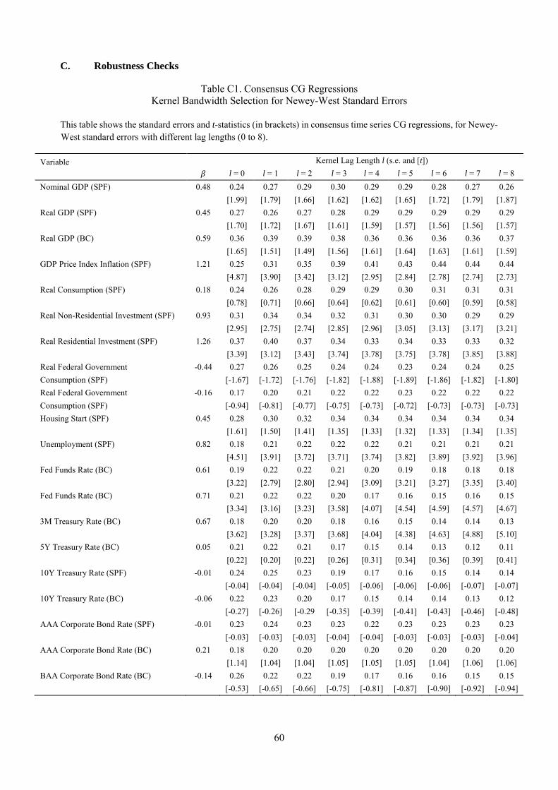
60

C. Robustness Checks

Table C1. Consensus CG Regressions Kernel Bandwidth Selection for Newey-West Standard Errors

This table shows the standard errors and t-statistics (in brackets) in consensus time series CG regressions, for Newey-West standard errors with different lag lengths (0 to 8).

Variable Kernel Lag Length l (s.e. and [t])

𝛽𝛽 l = 0 l = 1 l = 2 l = 3 l = 4 l = 5 l = 6 l = 7 l = 8 Nominal GDP (SPF) 0.48 0.24 0.27 0.29 0.30 0.29 0.29 0.28 0.27 0.26 [1.99] [1.79] [1.66] [1.62] [1.62] [1.65] [1.72] [1.79] [1.87] Real GDP (SPF) 0.45 0.27 0.26 0.27 0.28 0.29 0.29 0.29 0.29 0.29 [1.70] [1.72] [1.67] [1.61] [1.59] [1.57] [1.56] [1.56] [1.57] Real GDP (BC) 0.59 0.36 0.39 0.39 0.38 0.36 0.36 0.36 0.36 0.37 [1.65] [1.51] [1.49] [1.56] [1.61] [1.64] [1.63] [1.61] [1.59] GDP Price Index Inflation (SPF) 1.21 0.25 0.31 0.35 0.39 0.41 0.43 0.44 0.44 0.44 [4.87] [3.90] [3.42] [3.12] [2.95] [2.84] [2.78] [2.74] [2.73] Real Consumption (SPF) 0.18 0.24 0.26 0.28 0.29 0.29 0.30 0.31 0.31 0.31 [0.78] [0.71] [0.66] [0.64] [0.62] [0.61] [0.60] [0.59] [0.58] Real Non-Residential Investment (SPF) 0.93 0.31 0.34 0.34 0.32 0.31 0.30 0.30 0.29 0.29 [2.95] [2.75] [2.74] [2.85] [2.96] [3.05] [3.13] [3.17] [3.21] Real Residential Investment (SPF) 1.26 0.37 0.40 0.37 0.34 0.33 0.34 0.33 0.33 0.32 [3.39] [3.12] [3.43] [3.74] [3.78] [3.75] [3.78] [3.85] [3.88] Real Federal Government -0.44 0.27 0.26 0.25 0.24 0.24 0.23 0.24 0.24 0.25 Consumption (SPF) [-1.67] [-1.72] [-1.76] [-1.82] [-1.88] [-1.89] [-1.86] [-1.82] [-1.80] Real Federal Government -0.16 0.17 0.20 0.21 0.22 0.22 0.23 0.22 0.22 0.22 Consumption (SPF) [-0.94] [-0.81] [-0.77] [-0.75] [-0.73] [-0.72] [-0.73] [-0.73] [-0.73] Housing Start (SPF) 0.45 0.28 0.30 0.32 0.34 0.34 0.34 0.34 0.34 0.34 [1.61] [1.50] [1.41] [1.35] [1.33] [1.32] [1.33] [1.34] [1.35] Unemployment (SPF) 0.82 0.18 0.21 0.22 0.22 0.22 0.21 0.21 0.21 0.21 [4.51] [3.91] [3.72] [3.71] [3.74] [3.82] [3.89] [3.92] [3.96] Fed Funds Rate (BC) 0.61 0.19 0.22 0.22 0.21 0.20 0.19 0.18 0.18 0.18 [3.22] [2.79] [2.80] [2.94] [3.09] [3.21] [3.27] [3.35] [3.40] Fed Funds Rate (BC) 0.71 0.21 0.22 0.22 0.20 0.17 0.16 0.15 0.16 0.15 [3.34] [3.16] [3.23] [3.58] [4.07] [4.54] [4.59] [4.57] [4.67] 3M Treasury Rate (BC) 0.67 0.18 0.20 0.20 0.18 0.16 0.15 0.14 0.14 0.13 [3.62] [3.28] [3.37] [3.68] [4.04] [4.38] [4.63] [4.88] [5.10] 5Y Treasury Rate (BC) 0.05 0.21 0.22 0.21 0.17 0.15 0.14 0.13 0.12 0.11 [0.22] [0.20] [0.22] [0.26] [0.31] [0.34] [0.36] [0.39] [0.41] 10Y Treasury Rate (SPF) -0.01 0.24 0.25 0.23 0.19 0.17 0.16 0.15 0.14 0.14 [-0.04] [-0.04] [-0.04] [-0.05] [-0.06] [-0.06] [-0.06] [-0.07] [-0.07] 10Y Treasury Rate (BC) -0.06 0.22 0.23 0.20 0.17 0.15 0.14 0.14 0.13 0.12 [-0.27] [-0.26] [-0.29 [-0.35] [-0.39] [-0.41] [-0.43] [-0.46] [-0.48] AAA Corporate Bond Rate (SPF) -0.01 0.23 0.24 0.23 0.23 0.22 0.23 0.23 0.23 0.23 [-0.03] [-0.03] [-0.03] [-0.04] [-0.04] [-0.03] [-0.03] [-0.03] [-0.04] AAA Corporate Bond Rate (BC) 0.21 0.18 0.20 0.20 0.20 0.20 0.20 0.20 0.20 0.20 [1.14] [1.04] [1.04] [1.05] [1.05] [1.05] [1.04] [1.06] [1.06] BAA Corporate Bond Rate (BC) -0.14 0.26 0.22 0.22 0.19 0.17 0.16 0.16 0.15 0.15 [-0.53] [-0.65] [-0.66] [-0.75] [-0.81] [-0.87] [-0.90] [-0.92] [-0.94]

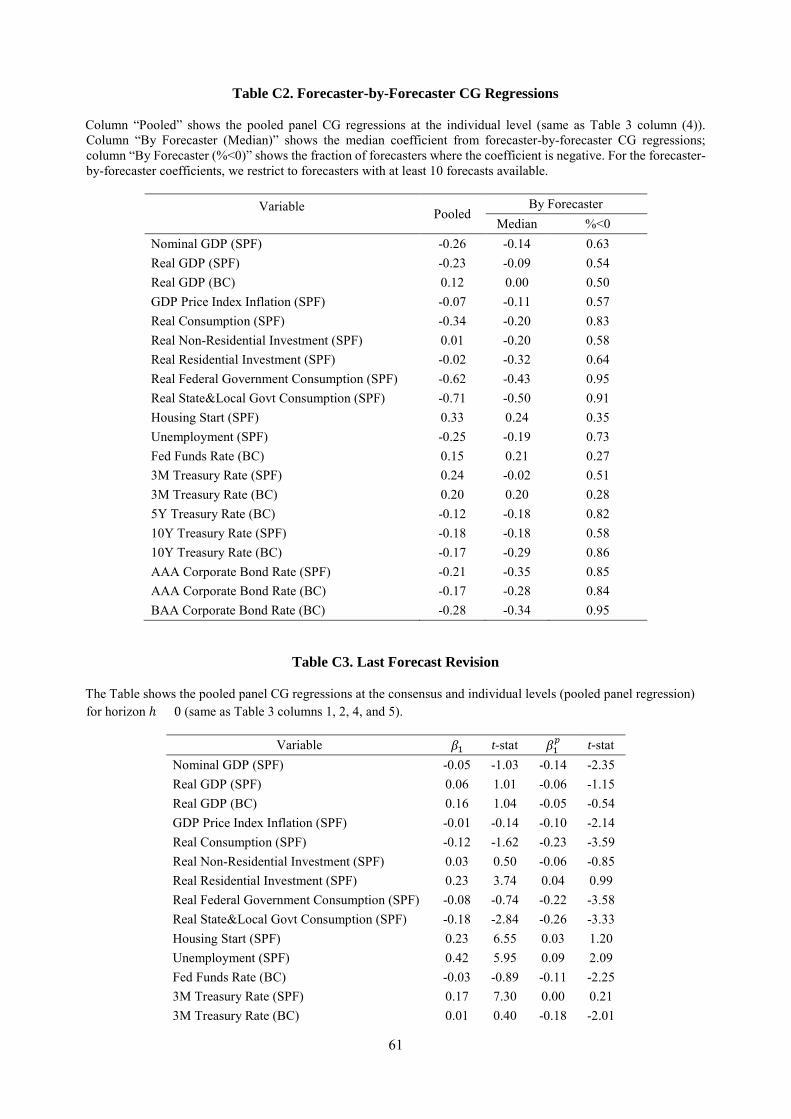
61

Table C2. Forecaster-by-Forecaster CG Regressions

Column “Pooled” shows the pooled panel CG regressions at the individual level (same as Table 3 column (4)). Column “By Forecaster (Median)” shows the median coefficient from forecaster-by-forecaster CG regressions; column “By Forecaster (%<0)” shows the fraction of forecasters where the coefficient is negative. For the forecaster-by-forecaster coefficients, we restrict to forecasters with at least 10 forecasts available.

Variable Pooled

By Forecaster Median %<0

Nominal GDP (SPF) -0.26 -0.14 0.63 Real GDP (SPF) -0.23 -0.09 0.54 Real GDP (BC) 0.12 0.00 0.50 GDP Price Index Inflation (SPF) -0.07 -0.11 0.57 Real Consumption (SPF) -0.34 -0.20 0.83 Real Non-Residential Investment (SPF) 0.01 -0.20 0.58 Real Residential Investment (SPF) -0.02 -0.32 0.64 Real Federal Government Consumption (SPF) -0.62 -0.43 0.95 Real State&Local Govt Consumption (SPF) -0.71 -0.50 0.91 Housing Start (SPF) 0.33 0.24 0.35 Unemployment (SPF) -0.25 -0.19 0.73 Fed Funds Rate (BC) 0.15 0.21 0.27 3M Treasury Rate (SPF) 0.24 -0.02 0.51 3M Treasury Rate (BC) 0.20 0.20 0.28 5Y Treasury Rate (BC) -0.12 -0.18 0.82 10Y Treasury Rate (SPF) -0.18 -0.18 0.58 10Y Treasury Rate (BC) -0.17 -0.29 0.86 AAA Corporate Bond Rate (SPF) -0.21 -0.35 0.85 AAA Corporate Bond Rate (BC) -0.17 -0.28 0.84 BAA Corporate Bond Rate (BC) -0.28 -0.34 0.95

Table C3. Last Forecast Revision

The Table shows the pooled panel CG regressions at the consensus and individual levels (pooled panel regression) for horizon ℎ = 0 (same as Table 3 columns 1, 2, 4, and 5).

Variable 𝛽𝛽1 t-stat 𝛽𝛽1𝑝𝑝 t-stat

Nominal GDP (SPF) -0.05 -1.03 -0.14 -2.35 Real GDP (SPF) 0.06 1.01 -0.06 -1.15 Real GDP (BC) 0.16 1.04 -0.05 -0.54 GDP Price Index Inflation (SPF) -0.01 -0.14 -0.10 -2.14 Real Consumption (SPF) -0.12 -1.62 -0.23 -3.59 Real Non-Residential Investment (SPF) 0.03 0.50 -0.06 -0.85 Real Residential Investment (SPF) 0.23 3.74 0.04 0.99 Real Federal Government Consumption (SPF) -0.08 -0.74 -0.22 -3.58 Real State&Local Govt Consumption (SPF) -0.18 -2.84 -0.26 -3.33 Housing Start (SPF) 0.23 6.55 0.03 1.20 Unemployment (SPF) 0.42 5.95 0.09 2.09 Fed Funds Rate (BC) -0.03 -0.89 -0.11 -2.25 3M Treasury Rate (SPF) 0.17 7.30 0.00 0.21 3M Treasury Rate (BC) 0.01 0.40 -0.18 -2.01

62

5Y Treasury Rate (BC) 0.12 3.27 0.00 0.04 10Y Treasury Rate (SPF) 0.15 3.34 -0.05 -1.86 10Y Treasury Rate (BC) 0.04 1.50 -0.01 -0.52 AAA Corporate Bond Rate (SPF) 0.07 1.29 -0.10 -2.15 AAA Corporate Bond Rate (BC) -0.10 -2.46 -0.16 -4.74 BAA Corporate Bond Rate (BC) 0.04 1.26 -0.09 -3.43

D. Non-Normal Shocks and Particle Filtering

In the main text, we assume that both the innovations of the latent process, 𝑢𝑢𝑡𝑡, and the measurement

error for each expert, 𝜖𝜖𝑡𝑡, follow normal distributions. In this case, as all the posterior distributions are

normal, the Kalman filter provides the closed form expression for the posterior densities. However, many

processes for macro and financial variables may have heavy tails and more closely follow, for example, a

𝑡𝑡-distribution. In this appendix, we relax the normality assumption and verify the model predictions with

fundamental shocks following fat tailed t-distributions.

In the non-normal case, while the point estimates of the Kalman filter still minimize mean-squared

error (MSE), the mean and covariance estimates of the filter are no longer sufficient to determine the

posterior distribution. Given that our formulation of diagnostic expectations involves a reweighting of the

likelihood function, we require more than the posterior mean and variance to properly compute the

diagnostic expectation distribution. Accordingly, we apply particle filtering to analyze expectations under

non-normal shocks.

D.1 Particle Filtering: Motivation and Set-Up

We start with the processes in Equations (3) and (4):

𝑠𝑠𝑡𝑡𝑖𝑖 = 𝑥𝑥𝑡𝑡 + 𝜖𝜖𝑡𝑡𝑖𝑖, 𝑥𝑥𝑡𝑡 = 𝜌𝜌𝑥𝑥𝑡𝑡−1 + 𝑢𝑢𝑡𝑡

where 𝑥𝑥𝑡𝑡 is the fundamental process and 𝑠𝑠𝑡𝑡𝑖𝑖 is forecaster 𝑑𝑑’s noisy signal. In Section 3, the shocks to these

processes are assumed to be normal. In the following, we analyze the case where the shock to the

fundamental process 𝑢𝑢𝑡𝑡 follows a t-distribution.

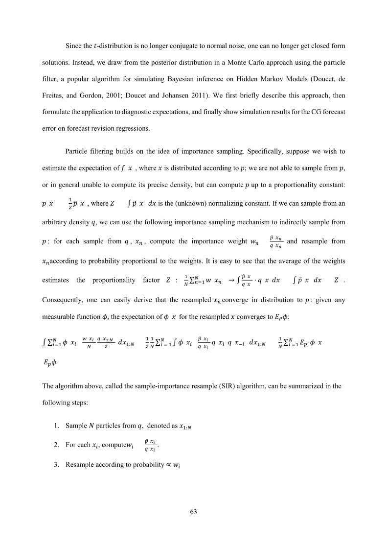
63

Since the 𝑡𝑡-distribution is no longer conjugate to normal noise, one can no longer get closed form

solutions. Instead, we draw from the posterior distribution in a Monte Carlo approach using the particle

filter, a popular algorithm for simulating Bayesian inference on Hidden Markov Models (Doucet, de

Freitas, and Gordon, 2001; Doucet and Johansen 2011). We first briefly describe this approach, then

formulate the application to diagnostic expectations, and finally show simulation results for the CG forecast

error on forecast revision regressions.

Particle filtering builds on the idea of importance sampling. Specifically, suppose we wish to

estimate the expectation of 𝑓𝑓(𝑥𝑥), where 𝑥𝑥 is distributed according to 𝑝𝑝; we are not able to sample from 𝑝𝑝,

or in general unable to compute its precise density, but can compute 𝑝𝑝 up to a proportionality constant:

𝑝𝑝(𝑥𝑥) = 1𝑍𝑍𝑝𝑝�(𝑥𝑥), where 𝑍𝑍 = ∫𝑝𝑝�(𝑥𝑥) 𝑑𝑑𝑥𝑥 is the (unknown) normalizing constant. If we can sample from an

arbitrary density 𝑞𝑞, we can use the following importance sampling mechanism to indirectly sample from

𝑝𝑝 : for each sample from 𝑞𝑞 , 𝑥𝑥𝑛𝑛 , compute the importance weight 𝑤𝑤𝑛𝑛 = 𝑝𝑝�(𝑥𝑥𝑛𝑛)𝑞𝑞(𝑥𝑥𝑛𝑛)

and resample from

𝑥𝑥𝑛𝑛according to probability proportional to the weights. It is easy to see that the average of the weights

estimates the proportionality factor 𝑍𝑍 : 1𝑁𝑁∑ 𝑤𝑤(𝑥𝑥𝑛𝑛)𝑁𝑁𝑛𝑛=1 → ∫𝑝𝑝�(𝑥𝑥)

𝑞𝑞(𝑥𝑥)⋅ 𝑞𝑞(𝑥𝑥)𝑑𝑑𝑥𝑥 = ∫𝑝𝑝�(𝑥𝑥) 𝑑𝑑𝑥𝑥 = 𝑍𝑍 .

Consequently, one can easily derive that the resampled 𝑥𝑥𝑛𝑛 converge in distribution to 𝑝𝑝 : given any

measurable function 𝜙𝜙, the expectation of 𝜙𝜙(𝑥𝑥)for the resampled 𝑥𝑥 converges to 𝐹𝐹𝑃𝑃𝜙𝜙:

∫∑ 𝜙𝜙(𝑥𝑥𝑖𝑖) 𝑤𝑤(𝑥𝑥𝑖𝑖)𝑁𝑁

𝑁𝑁𝑖𝑖=1

𝑞𝑞(𝑥𝑥1:𝑁𝑁)𝑍𝑍

𝑑𝑑𝑥𝑥1:𝑁𝑁 = 1𝑍𝑍1𝑁𝑁∑ ∫𝜙𝜙(𝑥𝑥𝑖𝑖) 𝑝𝑝�(𝑥𝑥𝑖𝑖)

𝑞𝑞(𝑥𝑥𝑖𝑖)𝑞𝑞(𝑥𝑥𝑖𝑖)𝑞𝑞(𝑥𝑥−𝑖𝑖) 𝑑𝑑𝑥𝑥1:𝑁𝑁

𝑁𝑁𝑖𝑖 = 1 = 1

𝑁𝑁∑ 𝐹𝐹𝑝𝑝[𝜙𝜙(𝑥𝑥)]𝑁𝑁𝑖𝑖 =1 =

𝐹𝐹𝑝𝑝𝜙𝜙

The algorithm above, called the sample-importance resample (SIR) algorithm, can be summarized in the

following steps:

1. Sample 𝑁𝑁 particles from 𝑞𝑞, denoted as 𝑥𝑥1:𝑁𝑁

2. For each 𝑥𝑥𝑖𝑖, compute𝑤𝑤𝑖𝑖 = 𝑝𝑝�(𝑥𝑥𝑖𝑖)𝑞𝑞(𝑥𝑥𝑖𝑖)

.

3. Resample according to probability ∝ 𝑤𝑤𝑖𝑖

64

For the hidden Markov Process model, the above idea generalizes to give us a quick algorithm to

sample from the filtering density 𝑝𝑝(𝑥𝑥𝑛𝑛|𝑠𝑠1:𝑛𝑛). Like the Kalman filter, the idea is to proceed inductively,

using the following forward equation:

𝑝𝑝(𝑥𝑥𝑛𝑛|𝑠𝑠1:𝑛𝑛) = 𝑔𝑔(𝑠𝑠𝑛𝑛|𝑥𝑥𝑛𝑛) 𝑝𝑝(𝑥𝑥𝑛𝑛|𝑠𝑠1:𝑛𝑛−1)

𝑝𝑝(𝑠𝑠𝑛𝑛| 𝑠𝑠1:𝑛𝑛−1) =

∫𝑔𝑔(𝑠𝑠𝑛𝑛|𝑥𝑥𝑛𝑛) 𝑓𝑓(𝑥𝑥𝑛𝑛|𝑥𝑥𝑛𝑛−1) 𝑝𝑝(𝑥𝑥𝑛𝑛−1|𝑠𝑠1:𝑛𝑛−1)𝑑𝑑𝑠𝑠1:𝑛𝑛−1𝑑𝑑𝑥𝑥𝑛𝑛−1𝑝𝑝(𝑠𝑠𝑛𝑛|𝑠𝑠1:𝑛𝑛−1)

By induction, suppose that we have samples from the previous filtered distribution 𝑝𝑝(𝑥𝑥𝑛𝑛−1|𝑠𝑠1:𝑛𝑛−1). Now,

given a (conditional) proposal 𝑞𝑞(𝑥𝑥𝑛𝑛|𝑥𝑥𝑛𝑛−1, 𝑠𝑠1:𝑛𝑛)for each sample, the recursive equality above suggests the

resampling weights: 𝑤𝑤(𝑥𝑥𝑛𝑛 | 𝑥𝑥𝑛𝑛−1) = 𝑔𝑔(𝑠𝑠𝑛𝑛|𝑥𝑥𝑛𝑛)𝑓𝑓(𝑥𝑥𝑛𝑛|𝑥𝑥𝑛𝑛−1)𝑞𝑞(𝑥𝑥𝑛𝑛 | 𝑥𝑥𝑛𝑛−1,𝑠𝑠1:𝑛𝑛)

. For the base case, where we have only seen the

data point 𝑠𝑠1, our filtered density 𝑝𝑝(𝑥𝑥1|𝑠𝑠1)is the standard Bayesian posterior, which can be sampled via

importance sampling.

The particle filter algorithm refers to this extension of the SIR algorithm to the sequential setting. The

procedure is as follows:

1. At time n = 1, generate 𝑁𝑁i.i.d. samples from a default proposal 𝑞𝑞.

2. Compute for each sample the weights 𝑤𝑤(𝑥𝑥𝑖𝑖) = 𝜇𝜇(𝑥𝑥𝑖𝑖) 𝑔𝑔(𝑠𝑠1 | 𝑥𝑥𝑖𝑖) 𝑞𝑞(𝑥𝑥𝑖𝑖)

3. Resample according to the weights, and store the sample.

4. For 𝑛𝑛 ≥ 2: for each 𝑥𝑥𝑛𝑛−1𝑖𝑖 in the sample, propose 𝑥𝑥𝑛𝑛𝑖𝑖 according to 𝑞𝑞(𝑥𝑥𝑛𝑛|𝑥𝑥𝑛𝑛−1 = 𝑥𝑥𝑖𝑖𝑛𝑛−1, 𝑠𝑠1:𝑛𝑛)

5. Compute for each 𝑥𝑥𝑛𝑛𝑖𝑖 the weights 𝑤𝑤(𝑥𝑥𝑛𝑛𝑖𝑖) = 𝑔𝑔(𝑠𝑠𝑛𝑛|𝑥𝑥𝑛𝑛𝑖𝑖) 𝑓𝑓(𝑥𝑥𝑛𝑛𝑖𝑖|𝑥𝑥𝑛𝑛−1𝑖𝑖)𝑞𝑞(𝑥𝑥𝑛𝑛|𝑥𝑥𝑛𝑛−1=𝑥𝑥𝑖𝑖𝑛𝑛−1,𝑠𝑠1:𝑛𝑛)

6. Resample according to the weights, save as 𝑥𝑥𝑛𝑛𝑖𝑖 .

Finally, we need to specify the proposal density 𝑞𝑞(𝑥𝑥𝑛𝑛|𝑥𝑥𝑛𝑛−1 = 𝑥𝑥𝑖𝑖𝑛𝑛−1, 𝑠𝑠1:𝑛𝑛). It is well-known that the

optimal proposal density should be the conditional distribution 𝑝𝑝(𝑥𝑥𝑛𝑛|𝑥𝑥𝑛𝑛−1 = 𝑥𝑥𝑖𝑖𝑛𝑛−1, 𝑠𝑠𝑛𝑛). If the latent

Markov process is a simple AR(1) process with normal innovation, one can analytically derive the optimal

proposal density 𝑝𝑝(𝑥𝑥𝑛𝑛|𝑥𝑥𝑛𝑛−1 = 𝑥𝑥𝑖𝑖𝑛𝑛−1, 𝑠𝑠𝑛𝑛).

𝑥𝑥𝑛𝑛|𝑥𝑥𝑛𝑛−1, 𝑠𝑠𝑛𝑛 ∼ 𝑁𝑁(𝜎𝜎𝜖𝜖2

𝜎𝜎𝜖𝜖2 + 𝜎𝜎𝑢𝑢2𝜌𝜌 𝑥𝑥𝑛𝑛−1 +

𝜎𝜎𝑢𝑢2

𝜎𝜎𝜖𝜖2 + 𝜎𝜎𝑢𝑢2 𝑠𝑠𝑛𝑛,

𝜎𝜎𝜖𝜖2𝜎𝜎𝑢𝑢2

𝜎𝜎𝜖𝜖2 + 𝜎𝜎𝑢𝑢2) = 𝑁𝑁(�̄�𝜇, �̄�𝛴)

65

While this result is only precise for normal processes, we shall still use �̄�𝜇, �̄�𝛴as location and scale parameters

for our proposal, which is now 𝑡𝑡-distributed. If the original innovations have 𝑑𝑑degrees of freedom, our

proposal will have 𝑑𝑑+22

degrees of freedom, which have much thicker tails.

D.2 Application to Diagnostic Expectations

To analyze the case of diagnostic expectations, we only need to re-adjust the resampling weights

by a simple likelihood ratio, as given by the following proposition:

Proposition D1 Let 𝑠𝑠∗(𝑠𝑠1:𝑛𝑛−1) be the predictive expectation of 𝑠𝑠𝑛𝑛 given 𝑠𝑠1:𝑛𝑛−1. The representativeness

𝑅𝑅(𝑥𝑥𝑛𝑛|𝑠𝑠1:𝑛𝑛) = 𝑝𝑝(𝑥𝑥𝑛𝑛| 𝑠𝑠1:𝑛𝑛)𝑝𝑝(𝑥𝑥𝑛𝑛| 𝑠𝑠1:𝑛𝑛−1,𝑠𝑠∗)

can be simplified to the likelihood ratio 𝑔𝑔(𝑠𝑠𝑛𝑛|𝑥𝑥𝑛𝑛)𝑔𝑔(𝑠𝑠∗|𝑥𝑥𝑛𝑛)

, up to a proportionality

constant independent of 𝑥𝑥𝑛𝑛.

Proof. By Bayes’ rule: 𝑅𝑅(𝑥𝑥𝑛𝑛|𝑠𝑠1:𝑛𝑛) = 𝑝𝑝(𝑥𝑥𝑛𝑛| 𝑠𝑠1:𝑛𝑛)𝑝𝑝(𝑥𝑥𝑛𝑛| 𝑠𝑠1:𝑛𝑛−1,𝑠𝑠∗)

= 𝑝𝑝(𝑠𝑠𝑛𝑛|𝑠𝑠1:𝑛𝑛−1,𝑥𝑥𝑛𝑛) ⋅𝑝𝑝(𝑥𝑥𝑛𝑛| 𝑠𝑠1:𝑛𝑛−1)𝑝𝑝(𝑠𝑠𝑛𝑛 | 𝑠𝑠1:𝑛𝑛−1)

⋅

(𝑝𝑝(𝑠𝑠∗ | 𝑠𝑠1:𝑛𝑛−1) ⋅𝑝𝑝(𝑥𝑥𝑛𝑛| 𝑠𝑠1:𝑛𝑛−1)𝑝𝑝(𝑠𝑠∗| 𝑠𝑠1:𝑛𝑛−1)

)−1.

Due to the Markov property, 𝑝𝑝(𝑠𝑠𝑛𝑛|𝑠𝑠1:𝑛𝑛−1,𝑥𝑥𝑛𝑛) = 𝑔𝑔(𝑠𝑠𝑛𝑛|𝑥𝑥𝑛𝑛) and 𝑝𝑝(𝑠𝑠𝑛𝑛 = 𝑠𝑠∗ |𝑠𝑠1:𝑛𝑛−1,𝑥𝑥𝑛𝑛) = 𝑔𝑔(𝑠𝑠∗|𝑥𝑥𝑛𝑛).

Plugging this in, we obtain:

𝑅𝑅(𝑥𝑥𝑛𝑛 |𝑠𝑠1:𝑛𝑛) = 𝑔𝑔(𝑠𝑠𝑛𝑛 | 𝑥𝑥𝑛𝑛) ⋅ 𝑝𝑝(𝑥𝑥𝑛𝑛|𝑠𝑠1:𝑛𝑛−1)

𝑝𝑝(𝑠𝑠𝑛𝑛|𝑠𝑠1:𝑛𝑛−1)⋅ (𝑔𝑔(𝑠𝑠∗|𝑥𝑥𝑛𝑛) ⋅ 𝑝𝑝(𝑥𝑥𝑛𝑛 | 𝑠𝑠1:𝑛𝑛−1)

𝑝𝑝(𝑠𝑠∗|𝑠𝑠1:𝑛𝑛−1))−1 =

𝑔𝑔(𝑠𝑠𝑛𝑛|𝑥𝑥𝑛𝑛)𝑔𝑔(𝑠𝑠∗ |𝑥𝑥𝑛𝑛)

⋅𝑝𝑝(𝑠𝑠∗|𝑠𝑠1:𝑛𝑛−1)𝑝𝑝(𝑠𝑠𝑛𝑛|𝑠𝑠1:𝑛𝑛−1)

The latter term 𝑝𝑝(𝑠𝑠∗|𝑠𝑠1:𝑛𝑛−1)𝑝𝑝(𝑠𝑠𝑛𝑛|𝑠𝑠1:𝑛𝑛−1)

is constant with respect to 𝑥𝑥𝑛𝑛, as desired.

As we have assumed that 𝑔𝑔 is a normal density, the likelihood ratio simplifies to:

𝑅𝑅(𝑥𝑥𝑛𝑛|𝑠𝑠1:𝑛𝑛) ∝ 𝑒𝑒𝑥𝑥𝑝𝑝�−(𝑥𝑥𝑛𝑛 − 𝑠𝑠𝑛𝑛)2

2𝜎𝜎𝜖𝜖2 +

(𝑥𝑥𝑛𝑛 − 𝑠𝑠∗)2

2𝜎𝜎𝜖𝜖2� = 𝑒𝑒𝑥𝑥𝑝𝑝 �

(𝑠𝑠𝑛𝑛 − 𝑠𝑠∗)𝑥𝑥𝑛𝑛𝜎𝜎𝜖𝜖2

�

Hence, if the observed signal 𝑠𝑠𝑛𝑛 is greater than 𝑠𝑠∗(a positive news), the forecaster puts an exponentially

heavier weight on larger values of 𝑥𝑥𝑛𝑛, and for negative news, he overweights smaller values of 𝑥𝑥𝑛𝑛, which

is in line with over-reaction to most recent news.

66

With the particle filter, we get the exponential reweighting by multiplying the original weights

𝑤𝑤(𝑥𝑥𝑛𝑛𝑖𝑖) = 𝑔𝑔(𝑠𝑠𝑛𝑛|𝑥𝑥𝑛𝑛𝑖𝑖) 𝑓𝑓(𝑥𝑥𝑛𝑛𝑖𝑖|𝑥𝑥𝑛𝑛−1𝑖𝑖)𝑞𝑞(𝑥𝑥𝑛𝑛|𝑥𝑥𝑛𝑛−1=𝑥𝑥𝑖𝑖𝑛𝑛−1,𝑠𝑠1:𝑛𝑛)

with the extra exponential factor 𝑒𝑒𝑥𝑥𝑝𝑝((𝑠𝑠𝑛𝑛 − 𝑠𝑠∗)𝑥𝑥𝑛𝑛𝜎𝜎𝜖𝜖2

) . As with the basic

particle filter algorithm discussed above, we need to specify our proposal density 𝑞𝑞 to target regions of

high density. We would like to target 𝑞𝑞� ∝ 𝑒𝑒𝑥𝑥𝑝𝑝((𝑠𝑠𝑛𝑛 − 𝑠𝑠∗)𝑥𝑥𝑛𝑛𝜎𝜎𝜖𝜖2

)𝑝𝑝(𝑥𝑥𝑛𝑛|𝑥𝑥𝑛𝑛−1,𝑠𝑠𝑛𝑛), which we estimate by first

assuming the normal model. Given that 𝑥𝑥𝑛𝑛|𝑥𝑥𝑛𝑛−1, 𝑠𝑠𝑛𝑛 ∼ 𝑁𝑁(�̄�𝜇, �̄�𝛴) in the normal model, the diagnostic

expectation is given by a shift of the posterior density by 𝜃𝜃⋅�̄�𝛴⋅(𝑠𝑠𝑛𝑛− 𝑠𝑠∗)𝜎𝜎𝜖𝜖2

. Thus we set the location and scale

parameter of our proposals as 𝜇𝜇𝑑𝑑𝑖𝑖𝑑𝑑𝑔𝑔 = �̄�𝜇 + 𝜃𝜃⋅�̄�𝛴(𝑠𝑠𝑛𝑛− 𝑠𝑠∗)𝜎𝜎𝜖𝜖2

, 𝛴𝛴𝑑𝑑𝑖𝑖𝑑𝑑𝑔𝑔 = �̄�𝛴, where �̄�𝜇, �̄�𝛴 are the location and scale

parameters for our original proposal. As before, we have 𝑑𝑑𝑓𝑓𝑞𝑞 = 𝑑𝑑𝑓𝑓 + 22

to ensure that our proposal has

heavier tails than the target distribution. To summarize, the algorithm is as follows:

1. From the original particle filter, estimate 𝑠𝑠∗ = 𝜌𝜌𝜇𝜇𝑛𝑛−1, with 𝜇𝜇𝑛𝑛−1 our predictive mean

𝐹𝐹[𝑥𝑥𝑛𝑛−1| 𝑠𝑠1:𝑛𝑛−1], estimated by the mean of our particles 𝑥𝑥𝑖𝑖𝑛𝑛−1.

2. Propose according to a 𝑡𝑡-distribution with location parameter 𝜇𝜇𝑑𝑑𝑖𝑖𝑑𝑑𝑔𝑔 = �̄�𝜇 + 𝜃𝜃⋅�̄�𝛴(𝑠𝑠𝑛𝑛− 𝑠𝑠∗)𝜎𝜎𝜖𝜖2

, 𝛴𝛴𝑑𝑑𝑖𝑖𝑑𝑑𝑔𝑔 =

�̄�𝛴, 𝑑𝑑𝑓𝑓𝑞𝑞 = 𝑑𝑑𝑓𝑓 + 22

.

3. For each proposal, resample with weights𝑤𝑤𝑑𝑑𝑖𝑖𝑑𝑑𝑔𝑔(𝑥𝑥𝑛𝑛|𝑥𝑥𝑛𝑛−1,𝑠𝑠𝑛𝑛) =

𝑔𝑔(𝑠𝑠𝑛𝑛|𝑥𝑥𝑛𝑛𝑖𝑖) 𝑓𝑓(𝑥𝑥𝑛𝑛𝑖𝑖|𝑥𝑥𝑛𝑛−1𝑖𝑖)𝑞𝑞(𝑥𝑥𝑛𝑛|𝑥𝑥𝑛𝑛−1=𝑥𝑥𝑖𝑖𝑛𝑛−1,𝑠𝑠1:𝑛𝑛)

𝑒𝑒𝑥𝑥𝑝𝑝((𝑠𝑠𝑛𝑛 − 𝑠𝑠∗)𝑥𝑥𝑛𝑛𝜎𝜎𝜖𝜖2

)

D.3 Results

In the simulations below, we set 𝜌𝜌 = 0.9,𝜎𝜎𝑢𝑢 = 0.2,𝜎𝜎𝜖𝜖 = 0.2, and 0 ≤ 𝜃𝜃 ≤ 1.5. We find that the

basic qualitative characteristics of diagnostic expectations are robust to fat tails. As Figure D1 shows, the

diagnostic expectation over-reacts to news, relative to the rational benchmark.

We then check the results of the CG forecast error on forecast revision regressions. Figure D2

shows the distribution of bootstrapped regression coefficients. Panel A first checks the case with normal

shocks, the particle filter simulation agrees with the predicted coefficients − 𝜃𝜃(1+𝜃𝜃)(1+𝜃𝜃)2+ 𝜃𝜃2 𝜌𝜌2

using the Kalman

filter. Panel B then shows the case where the shocks are heavy-tailed. We see that the coefficients for the

67

heavy-tailed shocks are more negative compared to the predicted values for the normal case. Specifically,

as the rational posterior exhibits heavier tail, the exponential reweighting of the diagnostic expectation

results in greater mass located on the extreme values of the exponential weight, and hence greater shift in

the diagnostic expectation. This effect is only present for diagnostic expectations — for rational

expectations i.e. 𝜃𝜃 = 0, we do not observe a divergence between normal and fat tailed distributions.

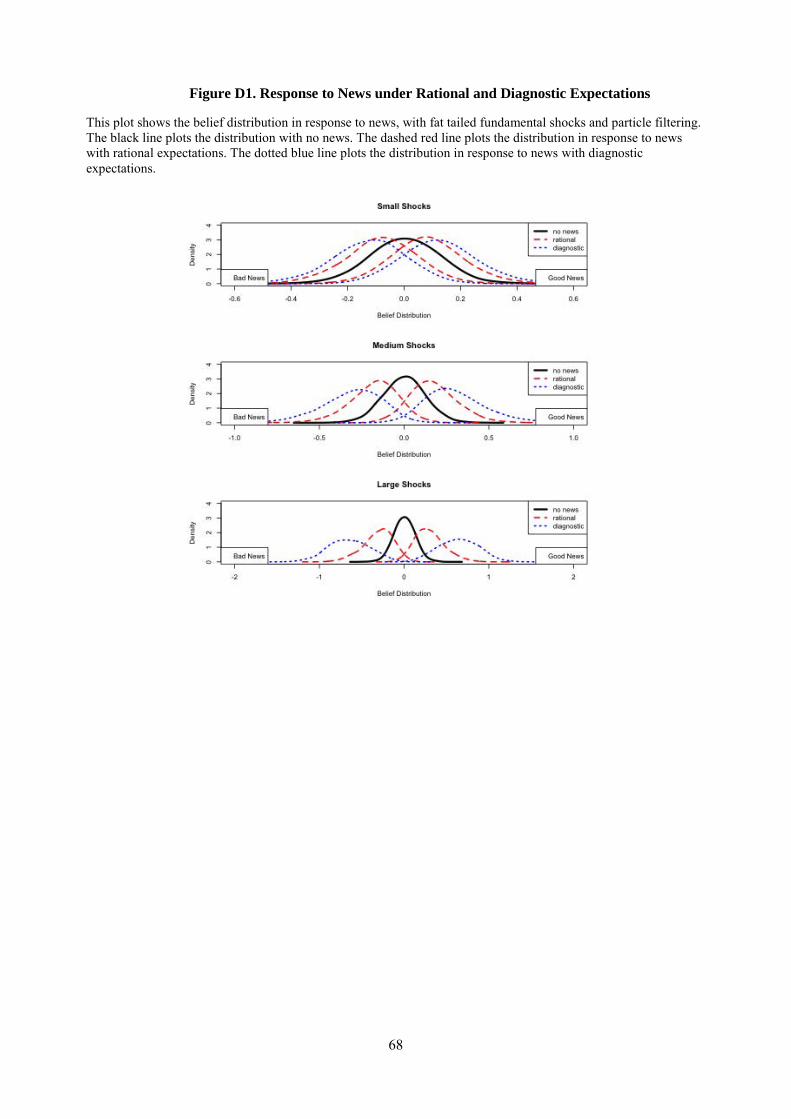
68

Figure D1. Response to News under Rational and Diagnostic Expectations

This plot shows the belief distribution in response to news, with fat tailed fundamental shocks and particle filtering. The black line plots the distribution with no news. The dashed red line plots the distribution in response to news with rational expectations. The dotted blue line plots the distribution in response to news with diagnostic expectations.

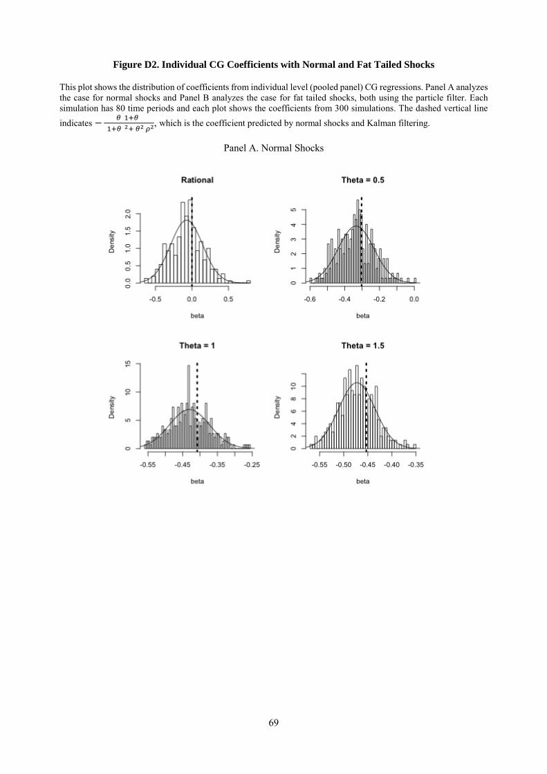
69

Figure D2. Individual CG Coefficients with Normal and Fat Tailed Shocks

This plot shows the distribution of coefficients from individual level (pooled panel) CG regressions. Panel A analyzes the case for normal shocks and Panel B analyzes the case for fat tailed shocks, both using the particle filter. Each simulation has 80 time periods and each plot shows the coefficients from 300 simulations. The dashed vertical line indicates − 𝜃𝜃(1+𝜃𝜃)

(1+𝜃𝜃)2+ 𝜃𝜃2 𝜌𝜌2, which is the coefficient predicted by normal shocks and Kalman filtering.

Panel A. Normal Shocks

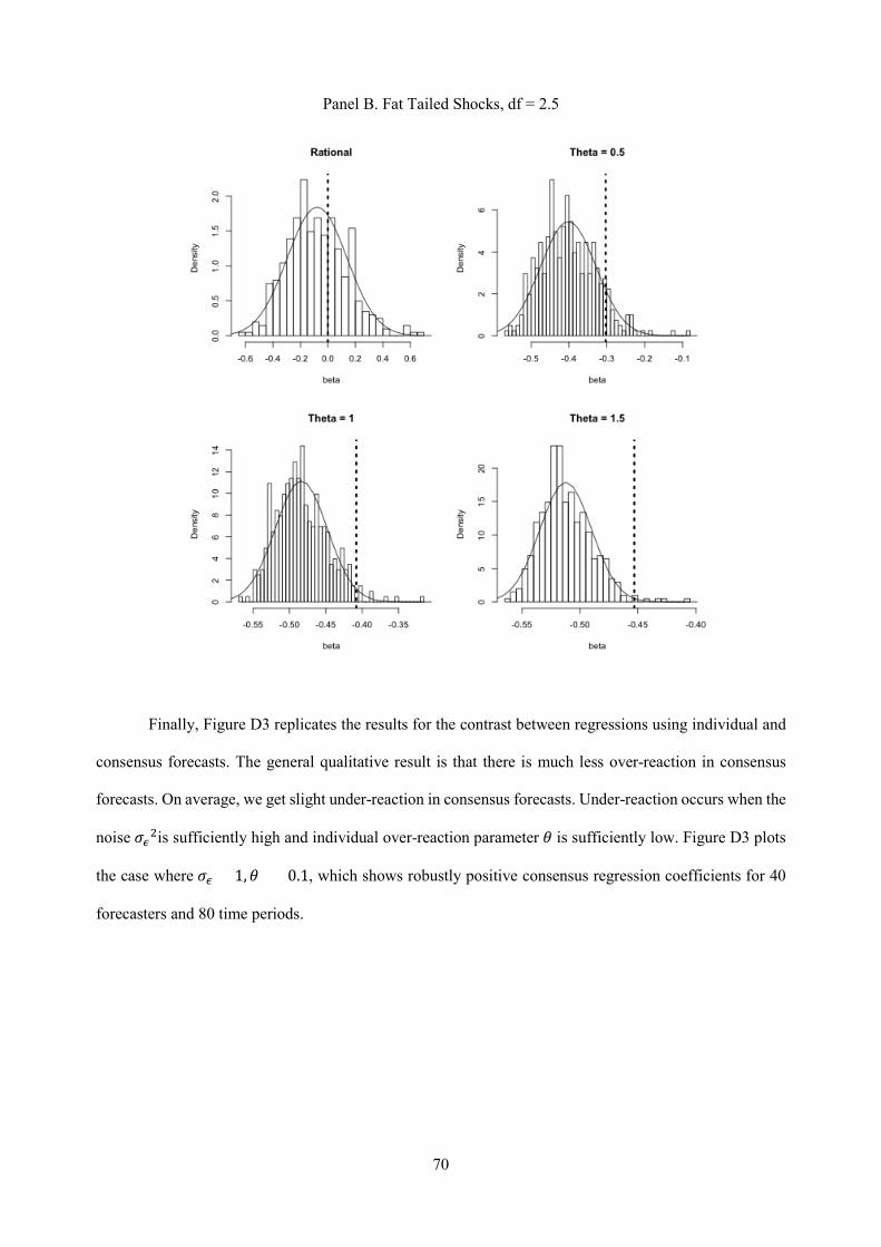
70

Panel B. Fat Tailed Shocks, df = 2.5

Finally, Figure D3 replicates the results for the contrast between regressions using individual and

consensus forecasts. The general qualitative result is that there is much less over-reaction in consensus

forecasts. On average, we get slight under-reaction in consensus forecasts. Under-reaction occurs when the

noise 𝜎𝜎𝜖𝜖2is sufficiently high and individual over-reaction parameter 𝜃𝜃 is sufficiently low. Figure D3 plots

the case where 𝜎𝜎𝜖𝜖 = 1,𝜃𝜃 = 0.1, which shows robustly positive consensus regression coefficients for 40

forecasters and 80 time periods.

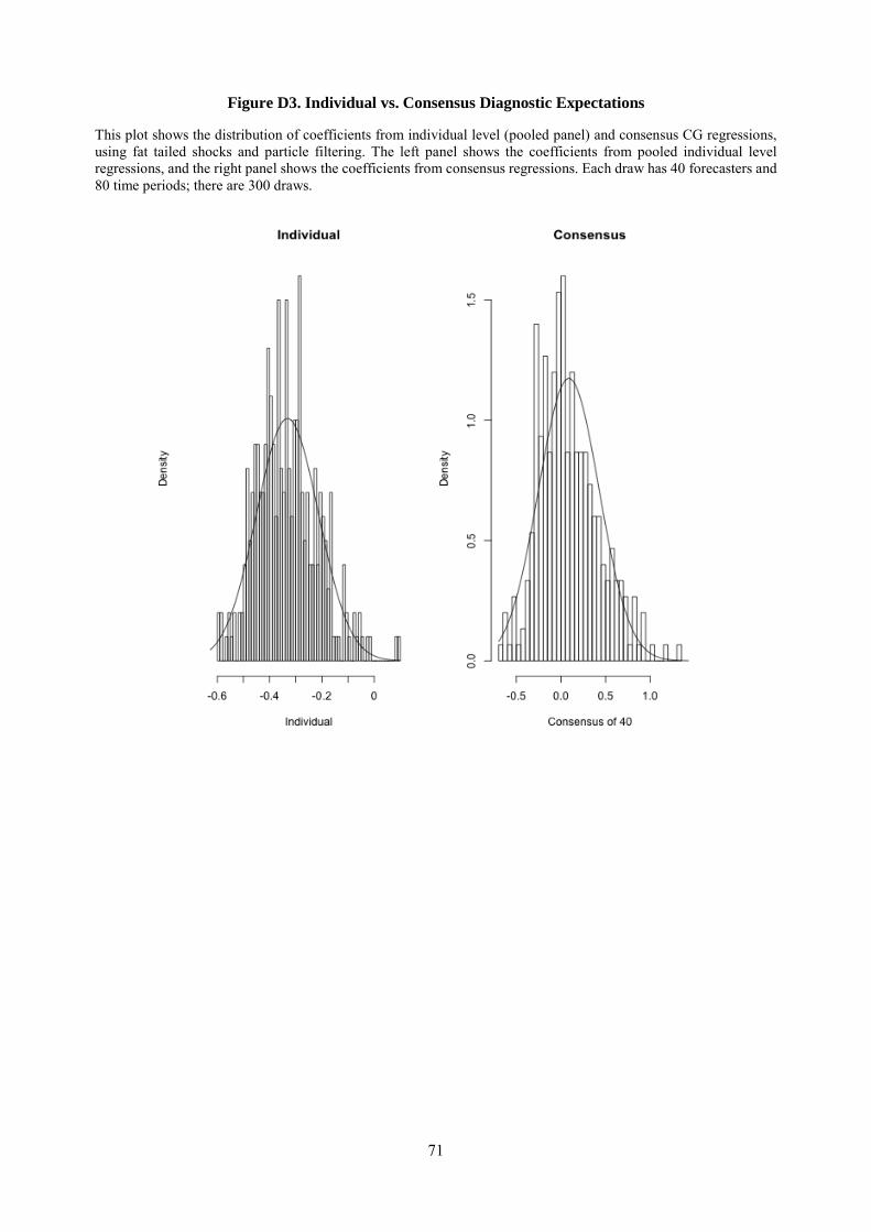
71

Figure D3. Individual vs. Consensus Diagnostic Expectations

This plot shows the distribution of coefficients from individual level (pooled panel) and consensus CG regressions, using fat tailed shocks and particle filtering. The left panel shows the coefficients from pooled individual level regressions, and the right panel shows the coefficients from consensus regressions. Each draw has 40 forecasters and 80 time periods; there are 300 draws.

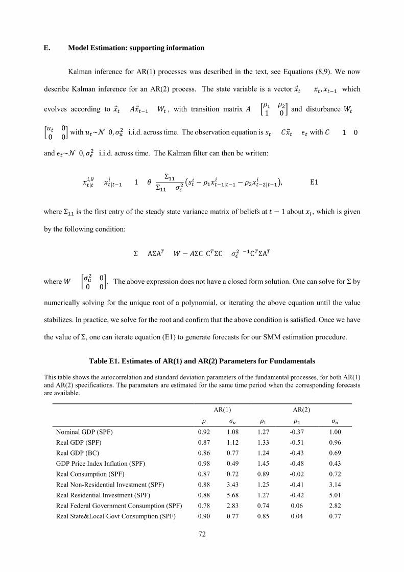
72

E. Model Estimation: supporting information

Kalman inference for AR(1) processes was described in the text, see Equations (8,9). We now

describe Kalman inference for an AR(2) process. The state variable is a vector �⃗�𝑥𝑡𝑡 = (𝑥𝑥𝑡𝑡, 𝑥𝑥𝑡𝑡−1) which

evolves according to �⃗�𝑥𝑡𝑡 = 𝐴𝐴�⃗�𝑥𝑡𝑡−1 + 𝑊𝑊𝑡𝑡 , with transition matrix 𝐴𝐴 = �𝜌𝜌1 𝜌𝜌21 0 � and disturbance 𝑊𝑊𝑡𝑡 =

�𝑢𝑢𝑡𝑡 00 0� with 𝑢𝑢𝑡𝑡~𝒩𝒩(0,𝜎𝜎𝑢𝑢2) i.i.d. across time. The observation equation is 𝑠𝑠𝑡𝑡 = 𝐵𝐵�⃗�𝑥𝑡𝑡 + 𝜖𝜖𝑡𝑡 with 𝐵𝐵 = [1 0]

and 𝜖𝜖𝑡𝑡~𝒩𝒩(0,𝜎𝜎𝜖𝜖2) i.i.d. across time. The Kalman filter can then be written:

𝑥𝑥𝑡𝑡|𝑡𝑡𝑖𝑖,𝜃𝜃 = 𝑥𝑥𝑡𝑡|𝑡𝑡−1

𝑖𝑖 + (1 + 𝜃𝜃)Σ11

Σ11 + 𝜎𝜎𝜖𝜖2�𝑠𝑠𝑡𝑡𝑖𝑖 − 𝜌𝜌1𝑥𝑥𝑡𝑡−1|𝑡𝑡−1

𝑖𝑖 − 𝜌𝜌2𝑥𝑥𝑡𝑡−2|𝑡𝑡−1𝑖𝑖 �, (E1)

where Σ11 is the first entry of the steady state variance matrix of beliefs at 𝑡𝑡 − 1 about 𝑥𝑥𝑡𝑡, which is given

by the following condition:

Σ = AΣA𝑇𝑇 + 𝑊𝑊 −𝐴𝐴ΣC(C𝑇𝑇ΣC + 𝜎𝜎𝜖𝜖2)−1C𝑇𝑇ΣA𝑇𝑇

where 𝑊𝑊 = �𝜎𝜎𝑢𝑢2 0

0 0�. The above expression does not have a closed form solution. One can solve for Σ by

numerically solving for the unique root of a polynomial, or iterating the above equation until the value

stabilizes. In practice, we solve for the root and confirm that the above condition is satisfied. Once we have

the value of Σ, one can iterate equation (E1) to generate forecasts for our SMM estimation procedure.

Table E1. Estimates of AR(1) and AR(2) Parameters for Fundamentals

This table shows the autocorrelation and standard deviation parameters of the fundamental processes, for both AR(1) and AR(2) specifications. The parameters are estimated for the same time period when the corresponding forecasts are available.

AR(1) AR(2) 𝜌𝜌 𝜎𝜎𝑢𝑢 𝜌𝜌1 𝜌𝜌2 𝜎𝜎𝑢𝑢

Nominal GDP (SPF) 0.92 1.08 1.27 -0.37 1.00 Real GDP (SPF) 0.87 1.12 1.33 -0.51 0.96 Real GDP (BC) 0.86 0.77 1.24 -0.43 0.69 GDP Price Index Inflation (SPF) 0.98 0.49 1.45 -0.48 0.43 Real Consumption (SPF) 0.87 0.72 0.89 -0.02 0.72 Real Non-Residential Investment (SPF) 0.88 3.43 1.25 -0.41 3.14 Real Residential Investment (SPF) 0.88 5.68 1.27 -0.42 5.01 Real Federal Government Consumption (SPF) 0.78 2.83 0.74 0.06 2.82 Real State&Local Govt Consumption (SPF) 0.90 0.77 0.85 0.04 0.77

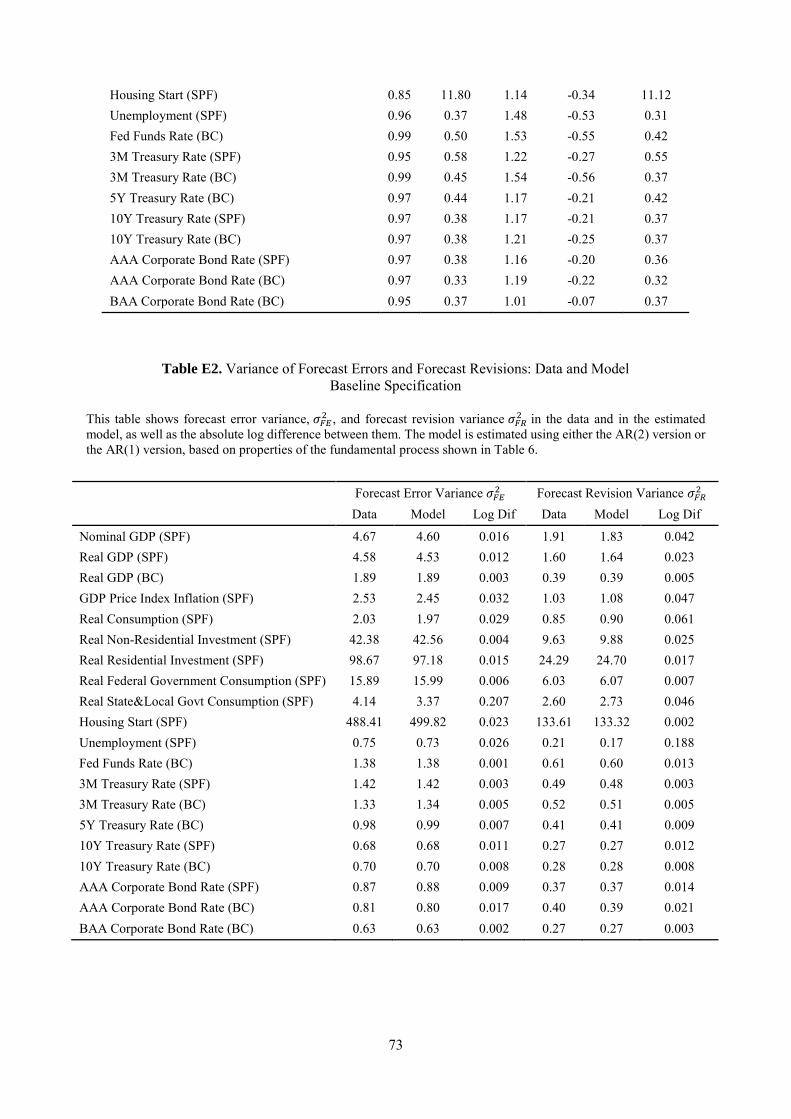
73

Housing Start (SPF) 0.85 11.80 1.14 -0.34 11.12 Unemployment (SPF) 0.96 0.37 1.48 -0.53 0.31 Fed Funds Rate (BC) 0.99 0.50 1.53 -0.55 0.42 3M Treasury Rate (SPF) 0.95 0.58 1.22 -0.27 0.55 3M Treasury Rate (BC) 0.99 0.45 1.54 -0.56 0.37 5Y Treasury Rate (BC) 0.97 0.44 1.17 -0.21 0.42 10Y Treasury Rate (SPF) 0.97 0.38 1.17 -0.21 0.37 10Y Treasury Rate (BC) 0.97 0.38 1.21 -0.25 0.37 AAA Corporate Bond Rate (SPF) 0.97 0.38 1.16 -0.20 0.36 AAA Corporate Bond Rate (BC) 0.97 0.33 1.19 -0.22 0.32 BAA Corporate Bond Rate (BC) 0.95 0.37 1.01 -0.07 0.37

Table E2. Variance of Forecast Errors and Forecast Revisions: Data and Model Baseline Specification

This table shows forecast error variance, 𝜎𝜎𝐹𝐹𝐹𝐹2 , and forecast revision variance 𝜎𝜎𝐹𝐹𝐴𝐴2 in the data and in the estimated model, as well as the absolute log difference between them. The model is estimated using either the AR(2) version or the AR(1) version, based on properties of the fundamental process shown in Table 6.

Forecast Error Variance 𝜎𝜎𝐹𝐹𝐹𝐹2 Forecast Revision Variance 𝜎𝜎𝐹𝐹𝐴𝐴2 Data Model Log Dif Data Model Log Dif

Nominal GDP (SPF) 4.67 4.60 0.016 1.91 1.83 0.042 Real GDP (SPF) 4.58 4.53 0.012 1.60 1.64 0.023 Real GDP (BC) 1.89 1.89 0.003 0.39 0.39 0.005 GDP Price Index Inflation (SPF) 2.53 2.45 0.032 1.03 1.08 0.047 Real Consumption (SPF) 2.03 1.97 0.029 0.85 0.90 0.061 Real Non-Residential Investment (SPF) 42.38 42.56 0.004 9.63 9.88 0.025 Real Residential Investment (SPF) 98.67 97.18 0.015 24.29 24.70 0.017 Real Federal Government Consumption (SPF) 15.89 15.99 0.006 6.03 6.07 0.007 Real State&Local Govt Consumption (SPF) 4.14 3.37 0.207 2.60 2.73 0.046 Housing Start (SPF) 488.41 499.82 0.023 133.61 133.32 0.002 Unemployment (SPF) 0.75 0.73 0.026 0.21 0.17 0.188 Fed Funds Rate (BC) 1.38 1.38 0.001 0.61 0.60 0.013 3M Treasury Rate (SPF) 1.42 1.42 0.003 0.49 0.48 0.003 3M Treasury Rate (BC) 1.33 1.34 0.005 0.52 0.51 0.005 5Y Treasury Rate (BC) 0.98 0.99 0.007 0.41 0.41 0.009 10Y Treasury Rate (SPF) 0.68 0.68 0.011 0.27 0.27 0.012 10Y Treasury Rate (BC) 0.70 0.70 0.008 0.28 0.28 0.008 AAA Corporate Bond Rate (SPF) 0.87 0.88 0.009 0.37 0.37 0.014 AAA Corporate Bond Rate (BC) 0.81 0.80 0.017 0.40 0.39 0.021 BAA Corporate Bond Rate (BC) 0.63 0.63 0.002 0.27 0.27 0.003

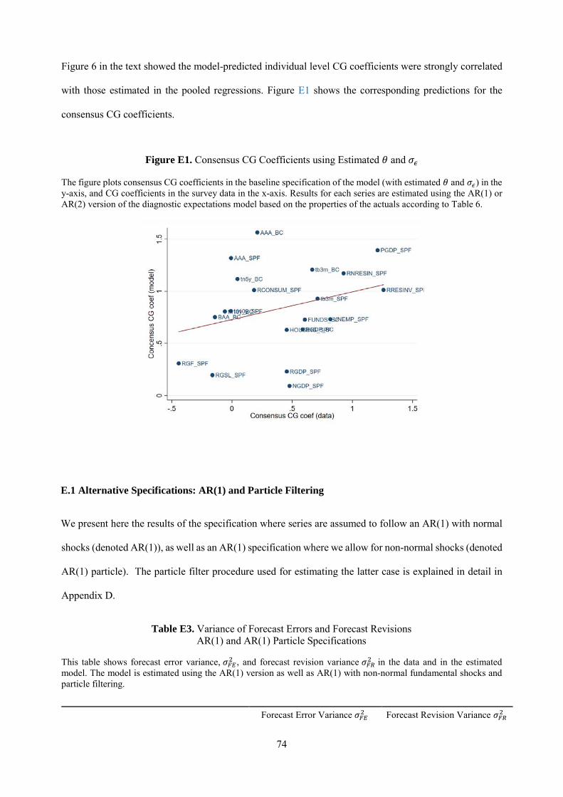
74

Figure 6 in the text showed the model-predicted individual level CG coefficients were strongly correlated

with those estimated in the pooled regressions. Figure E1 shows the corresponding predictions for the

consensus CG coefficients.

Figure E1. Consensus CG Coefficients using Estimated 𝜃𝜃 and 𝜎𝜎𝜖𝜖

The figure plots consensus CG coefficients in the baseline specification of the model (with estimated 𝜃𝜃 and 𝜎𝜎𝜖𝜖) in the y-axis, and CG coefficients in the survey data in the x-axis. Results for each series are estimated using the AR(1) or AR(2) version of the diagnostic expectations model based on the properties of the actuals according to Table 6.

E.1 Alternative Specifications: AR(1) and Particle Filtering

We present here the results of the specification where series are assumed to follow an AR(1) with normal

shocks (denoted AR(1)), as well as an AR(1) specification where we allow for non-normal shocks (denoted

AR(1) particle). The particle filter procedure used for estimating the latter case is explained in detail in

Appendix D.

Table E3. Variance of Forecast Errors and Forecast Revisions AR(1) and AR(1) Particle Specifications

This table shows forecast error variance, 𝜎𝜎𝐹𝐹𝐹𝐹2 , and forecast revision variance 𝜎𝜎𝐹𝐹𝐴𝐴2 in the data and in the estimated model. The model is estimated using the AR(1) version as well as AR(1) with non-normal fundamental shocks and particle filtering.

Forecast Error Variance 𝜎𝜎𝐹𝐹𝐹𝐹2 Forecast Revision Variance 𝜎𝜎𝐹𝐹𝐴𝐴2

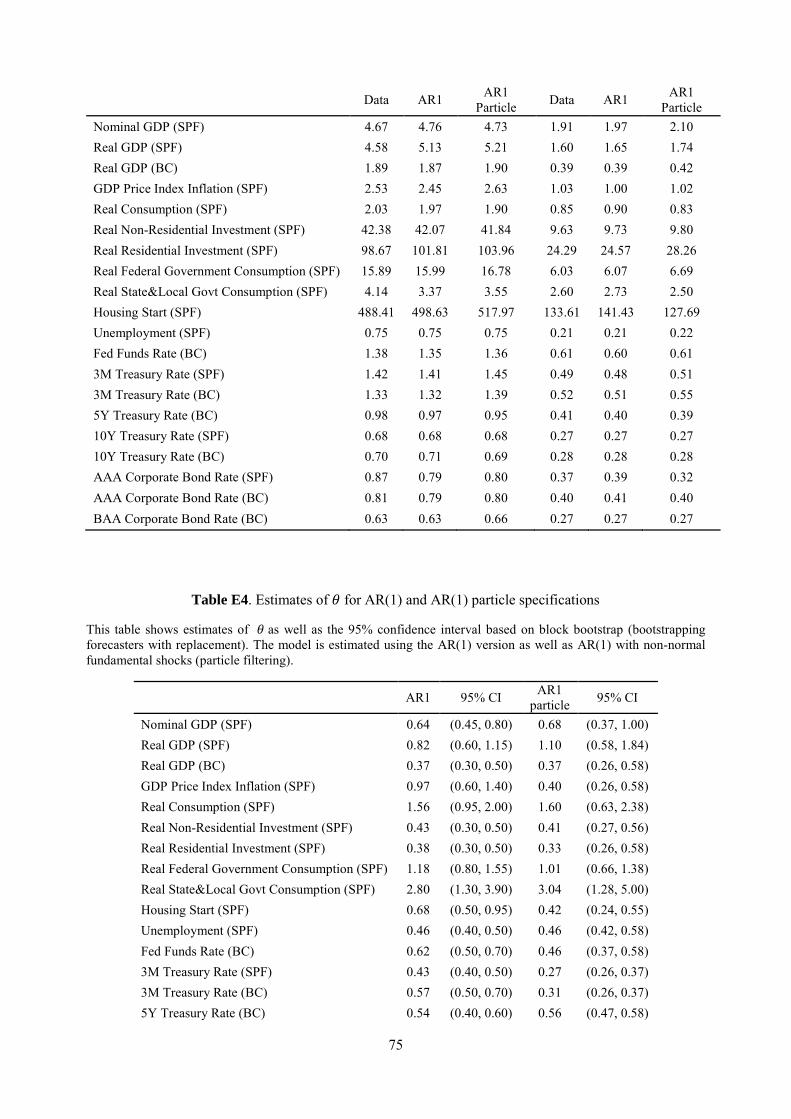
75

Table E4. Estimates of 𝜃𝜃 for AR(1) and AR(1) particle specifications

This table shows estimates of 𝜃𝜃 as well as the 95% confidence interval based on block bootstrap (bootstrapping forecasters with replacement). The model is estimated using the AR(1) version as well as AR(1) with non-normal fundamental shocks (particle filtering).

AR1 95% CI AR1 particle 95% CI

Nominal GDP (SPF) 0.64 (0.45, 0.80) 0.68 (0.37, 1.00) Real GDP (SPF) 0.82 (0.60, 1.15) 1.10 (0.58, 1.84) Real GDP (BC) 0.37 (0.30, 0.50) 0.37 (0.26, 0.58) GDP Price Index Inflation (SPF) 0.97 (0.60, 1.40) 0.40 (0.26, 0.58) Real Consumption (SPF) 1.56 (0.95, 2.00) 1.60 (0.63, 2.38) Real Non-Residential Investment (SPF) 0.43 (0.30, 0.50) 0.41 (0.27, 0.56) Real Residential Investment (SPF) 0.38 (0.30, 0.50) 0.33 (0.26, 0.58) Real Federal Government Consumption (SPF) 1.18 (0.80, 1.55) 1.01 (0.66, 1.38) Real State&Local Govt Consumption (SPF) 2.80 (1.30, 3.90) 3.04 (1.28, 5.00) Housing Start (SPF) 0.68 (0.50, 0.95) 0.42 (0.24, 0.55) Unemployment (SPF) 0.46 (0.40, 0.50) 0.46 (0.42, 0.58) Fed Funds Rate (BC) 0.62 (0.50, 0.70) 0.46 (0.37, 0.58) 3M Treasury Rate (SPF) 0.43 (0.40, 0.50) 0.27 (0.26, 0.37) 3M Treasury Rate (BC) 0.57 (0.50, 0.70) 0.31 (0.26, 0.37) 5Y Treasury Rate (BC) 0.54 (0.40, 0.60) 0.56 (0.47, 0.58)

Data AR1 AR1 Particle Data AR1 AR1

Particle Nominal GDP (SPF) 4.67 4.76 4.73 1.91 1.97 2.10 Real GDP (SPF) 4.58 5.13 5.21 1.60 1.65 1.74 Real GDP (BC) 1.89 1.87 1.90 0.39 0.39 0.42 GDP Price Index Inflation (SPF) 2.53 2.45 2.63 1.03 1.00 1.02 Real Consumption (SPF) 2.03 1.97 1.90 0.85 0.90 0.83 Real Non-Residential Investment (SPF) 42.38 42.07 41.84 9.63 9.73 9.80 Real Residential Investment (SPF) 98.67 101.81 103.96 24.29 24.57 28.26 Real Federal Government Consumption (SPF) 15.89 15.99 16.78 6.03 6.07 6.69 Real State&Local Govt Consumption (SPF) 4.14 3.37 3.55 2.60 2.73 2.50 Housing Start (SPF) 488.41 498.63 517.97 133.61 141.43 127.69 Unemployment (SPF) 0.75 0.75 0.75 0.21 0.21 0.22 Fed Funds Rate (BC) 1.38 1.35 1.36 0.61 0.60 0.61 3M Treasury Rate (SPF) 1.42 1.41 1.45 0.49 0.48 0.51 3M Treasury Rate (BC) 1.33 1.32 1.39 0.52 0.51 0.55 5Y Treasury Rate (BC) 0.98 0.97 0.95 0.41 0.40 0.39 10Y Treasury Rate (SPF) 0.68 0.68 0.68 0.27 0.27 0.27 10Y Treasury Rate (BC) 0.70 0.71 0.69 0.28 0.28 0.28 AAA Corporate Bond Rate (SPF) 0.87 0.79 0.80 0.37 0.39 0.32 AAA Corporate Bond Rate (BC) 0.81 0.79 0.80 0.40 0.41 0.40 BAA Corporate Bond Rate (BC) 0.63 0.63 0.66 0.27 0.27 0.27

76

10Y Treasury Rate (SPF) 0.59 (0.50, 0.60) 0.56 (0.47, 0.58) 10Y Treasury Rate (BC) 0.55 (0.50, 0.60) 0.54 (0.47, 0.58) AAA Corporate Bond Rate (SPF) 0.76 (0.70, 0.90) 0.63 (0.47, 0.74) AAA Corporate Bond Rate (BC) 1.10 (0.90, 1.30) 1.10 (0.84, 1.24) BAA Corporate Bond Rate (BC) 0.73 (0.64, 0.80) 0.46 (0.38, 0.55)

Table E5. CG Coefficients: Data vs Model

This table shows regressions of CG coefficients in the data (LHS) on CG coefficients in the estimated model (RHS) across different series. The model is estimated using the baseline version (primarily AR(2)), the AR(1) version, and AR(1) with non-normal fundamental shocks (particle filtering). Panel A uses individual CG coefficient from forecaster-level panel regressions. Panel B uses consensus CG coefficient from time series regressions of consensus forecasts.

Panel A. Individual CG

Data CG (Individual) (1) (2) (3) Model CG (Baseline) 1.043*** (0.168) Model CG (AR1) 0.772*** (0.154) Model CG (AR1 particle) 0.706*** (0.152) Constant 0.0832* -0.0294 -0.0336 (0.0397) (0.0433) (0.0443) Observations 20 20 20 R-squared 0.686 0.605 0.561

Robust standard errors in parentheses *** p<0.01, ** p<0.05, * p<0.1

Panel B. Consensus CG

Data CG (Consensus) (1) (2) (3) Model CG (Baseline) 0.345 (0.260) Model CG (AR1) 0.138 (0.214) Model CG (AR1 particle) 0.342 (0.264) Constant 0.102 0.288 0.165 (0.222) (0.174) (0.195) Observations 20 20 20 R-squared 0.092 0.020 0.077

Robust standard errors in parentheses *** p<0.01, ** p<0.05, * p<0.1

77

E.2 Forecaster Level Results

Table 8 in Section 6 presents the pooled estimates of the latent parameters 𝜃𝜃𝑘𝑘 and 𝜎𝜎𝜖𝜖,𝑘𝑘 that were allowed

to vary by series k but not by individual forecaster. We also estimate the model at the individual level, and

obtain estimated parameters (𝜃𝜃𝑘𝑘𝑖𝑖 ,𝜎𝜎𝜖𝜖,𝑘𝑘𝑖𝑖 ) for each forecaster and a given series. Table E6 shows the median

estimates of these parameters at the individual level in the baseline specification of our model. Results are

similar using other specifications.

Table E6. Model Estimation Results by Forecaster This table shows the median of individual-level 𝜃𝜃𝑖𝑖 and 𝜎𝜎𝜖𝜖𝑖𝑖 (normalized by 𝜎𝜎𝑢𝑢) estimates, as well as the CG coefficients in the model with estimated 𝜃𝜃𝑖𝑖 and 𝜎𝜎𝜖𝜖𝑖𝑖 . For the model CG coefficients, we use the forecaster level estimates (𝜃𝜃𝑖𝑖, 𝜎𝜎𝜖𝜖𝑖𝑖), together with the fundamental process and its parameters, to generate model-implied forecasts for each forecaster and each time period where the forecaster is available; we then run panel CG regressions and consensus CG regressions using the model-based forecasts. Results for each series are estimated using the AR(1) or AR(2) version of the diagnostic expectations model based on the properties of the actuals according to Table 6.

Median 𝜃𝜃𝑖𝑖 Median 𝜎𝜎𝜖𝜖𝑖𝑖/𝜎𝜎𝑢𝑢 Individual CG Consensus CG

Nominal GDP (SPF) 0.32 1.08 -0.20 0.29 Real GDP (SPF) 0.69 0.78 -0.26 0.10 Real GDP (BC) 0.63 1.43 -0.30 0.35 GDP Price Index Inflation (SPF) 0.59 3.42 -0.25 1.06 Real Consumption (SPF) 0.64 2.71 -0.36 0.95 Real Non-Residential Investment (SPF) 0.44 1.55 -0.15 1.15 Real Residential Investment (SPF) 0.42 1.68 -0.22 0.90 Real Federal Government Consumption (SPF) 0.73 1.71 -0.36 0.11 Real State&Local Govt Consumption (SPF) 0.91 4.50 -0.47 0.38 Housing Start (SPF) 1.37 2.11 -0.42 0.60 Unemployment (SPF) -0.17 0.67 0.26 1.00 Fed Funds Rate (BC) -0.01 1.24 -0.04 0.61 3M Treasury Rate (SPF) 0.21 1.60 0.04 1.18 3M Treasury Rate (BC) -0.03 1.87 0.01 1.08 5Y Treasury Rate (BC) 0.37 2.49 -0.21 1.10 10Y Treasury Rate (SPF) 0.47 2.55 -0.35 0.68 10Y Treasury Rate (BC) 0.26 2.74 -0.30 0.88 AAA Corporate Bond Rate (SPF) 0.63 5.21 -0.36 1.20 AAA Corporate Bond Rate (BC) 0.76 5.20 -0.35 1.47 BAA Corporate Bond Rate (BC) 0.69 2.50 -0.36 0.70

Table E7 shows that there is a consistent correlation between individual level estimates of 𝜃𝜃𝑖𝑖 across series.

78

Table E7. Rank Correlations for 𝜃𝜃𝑖𝑖

This table shows the rank correlation for forecaster-level estimates of 𝜃𝜃𝑖𝑖 across different series, and p-value in parenthesis. Panel A shows results for series and forecasters in SPF. Panel B shows results for series and forecasters in Blue Chip. 𝜃𝜃𝑖𝑖 for each series is estimated using the AR(1) or AR(2) version of the diagnostic expectations model based on the properties of the actuals according to Table 6.

Panel A: SPF Series

NGDP RGDP PGDP RCONSUM RNRESINV RRESINV RGF RGSL HOUSING UNEMP tb3m tn10y RGDP 0.48 (0.000) PGDP -0.04 0.00 (0.747) (0.976) RCONSUM -0.20 -0.28 -0.11 (0.128) (0.030) (0.393) RNRESINV 0.41 0.34 -0.20 -0.11 (0.001) (0.008) (0.127) (0.382) RRESINV 0.29 0.13 -0.07 -0.01 0.25 (0.023) (0.326) (0.571) (0.919) (0.048) RGF -0.01 -0.26 -0.33 0.35 0.08 0.25 (0.938) (0.043) (0.010) (0.005) (0.539) (0.047) RGSL 0.00 -0.19 -0.17 0.50 0.04 -0.21 0.42 (0.984) (0.139) (0.199) (0.000) (0.745) (0.100) (0.001) HOUSING 0.08 -0.03 -0.09 0.02 0.18 0.45 0.02 -0.03 (0.518) (0.822) (0.487) (0.862) (0.170) (0.000) (0.899) (0.823) UNEMP -0.18 -0.10 0.04 0.11 -0.07 -0.01 0.11 -0.12 0.03 (0.159) (0.443) (0.754) (0.388) (0.581) (0.913) (0.392) (0.367) (0.814) tb3m 0.15 0.22 -0.01 -0.29 0.18 0.07 -0.29 -0.17 0.04 0.03 (0.233) (0.087) (0.944) (0.023) (0.158) (0.609) (0.023) (0.182) (0.732) (0.791) tn10y 0.09 -0.23 -0.03 0.16 -0.03 0.28 0.39 0.08 -0.09 0.00 -0.13 (0.495) (0.076) (0.846) (0.206) (0.799) (0.025) (0.002) (0.542) (0.489) (0.998) (0.332) AAA 0.15 0.13 0.21 -0.27 0.29 0.14 -0.19 -0.19 0.04 -0.02 0.36 -0.22

(0.249) (0.300) (0.102) (0.032) (0.021) (0.295) (0.132) (0.147) (0.745) (0.898) (0.004) (0.081)

Panel B: Blue Chip Series

RGDPBC FFBC tb3mBC tn5yBC tn10yBC AAABC

FFBC 0.13 (0.306)

tb3mBC 0.10 0.54 (0.450) (0.000)

tb5yBC 0.15 0.45 0.37 (0.243) (0.000) (0.003)

tn10yBC -0.32 0.02 -0.01 0.02 (0.010) (0.876) (0.956) (0.863)

AAABC -0.12 0.08 -0.03 0.15 0.20 (0.346) (0.530) (0.808) (0.247) (0.122)

BAABC -0.05 0.09 0.07 0.12 -0.13 0.12 (0.722) (0.480) (0.592) (0.332) (0.302) (0.352)

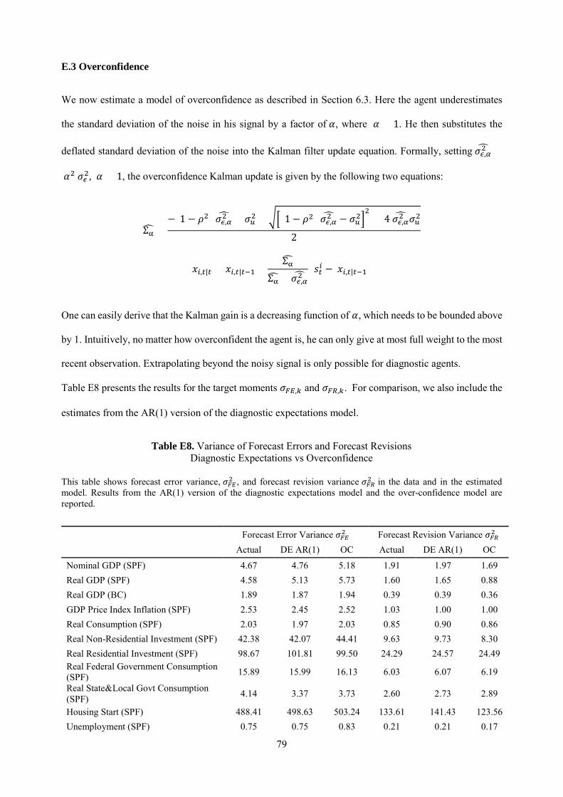
79

E.3 Overconfidence

We now estimate a model of overconfidence as described in Section 6.3. Here the agent underestimates

the standard deviation of the noise in his signal by a factor of 𝛼𝛼, where 𝛼𝛼 < 1. He then substitutes the

deflated standard deviation of the noise into the Kalman filter update equation. Formally, setting 𝜎𝜎𝜖𝜖,𝛼𝛼2� =

𝛼𝛼2 𝜎𝜎𝜖𝜖2, 𝛼𝛼 < 1, the overconfidence Kalman update is given by the following two equations:

Σα� =−(1 − 𝜌𝜌2) 𝜎𝜎𝜖𝜖,𝛼𝛼

2� + 𝜎𝜎𝑢𝑢2 + ��(1− 𝜌𝜌2) 𝜎𝜎𝜖𝜖,𝛼𝛼2� − 𝜎𝜎𝑢𝑢2�

2+ 4 𝜎𝜎𝜖𝜖,𝛼𝛼

2� 𝜎𝜎𝑢𝑢2

2

𝑥𝑥𝑖𝑖,𝑡𝑡|𝑡𝑡 = 𝑥𝑥𝑖𝑖,𝑡𝑡|𝑡𝑡−1 +Σα�

Σα� + 𝜎𝜎𝜖𝜖,𝛼𝛼2� (𝑠𝑠𝑡𝑡𝑖𝑖 − 𝑥𝑥𝑖𝑖,𝑡𝑡|𝑡𝑡−1)

One can easily derive that the Kalman gain is a decreasing function of 𝛼𝛼, which needs to be bounded above

by 1. Intuitively, no matter how overconfident the agent is, he can only give at most full weight to the most

recent observation. Extrapolating beyond the noisy signal is only possible for diagnostic agents.

Table E8 presents the results for the target moments 𝜎𝜎𝐹𝐹𝐹𝐹,𝑘𝑘 and 𝜎𝜎𝐹𝐹𝐴𝐴,𝑘𝑘. For comparison, we also include the

estimates from the AR(1) version of the diagnostic expectations model.

Table E8. Variance of Forecast Errors and Forecast Revisions Diagnostic Expectations vs Overconfidence

This table shows forecast error variance, 𝜎𝜎𝐹𝐹𝐹𝐹2 , and forecast revision variance 𝜎𝜎𝐹𝐹𝐴𝐴2 in the data and in the estimated model. Results from the AR(1) version of the diagnostic expectations model and the over-confidence model are reported.

Forecast Error Variance 𝜎𝜎𝐹𝐹𝐹𝐹2 Forecast Revision Variance 𝜎𝜎𝐹𝐹𝐴𝐴2 Actual DE AR(1) OC Actual DE AR(1) OC

Nominal GDP (SPF) 4.67 4.76 5.18 1.91 1.97 1.69 Real GDP (SPF) 4.58 5.13 5.73 1.60 1.65 0.88 Real GDP (BC) 1.89 1.87 1.94 0.39 0.39 0.36 GDP Price Index Inflation (SPF) 2.53 2.45 2.52 1.03 1.00 1.00 Real Consumption (SPF) 2.03 1.97 2.03 0.85 0.90 0.86 Real Non-Residential Investment (SPF) 42.38 42.07 44.41 9.63 9.73 8.30 Real Residential Investment (SPF) 98.67 101.81 99.50 24.29 24.57 24.49 Real Federal Government Consumption (SPF) 15.89 15.99 16.13 6.03 6.07 6.19

Real State&Local Govt Consumption (SPF) 4.14 3.37 3.73 2.60 2.73 2.89

Housing Start (SPF) 488.41 498.63 503.24 133.61 141.43 123.56 Unemployment (SPF) 0.75 0.75 0.83 0.21 0.21 0.17

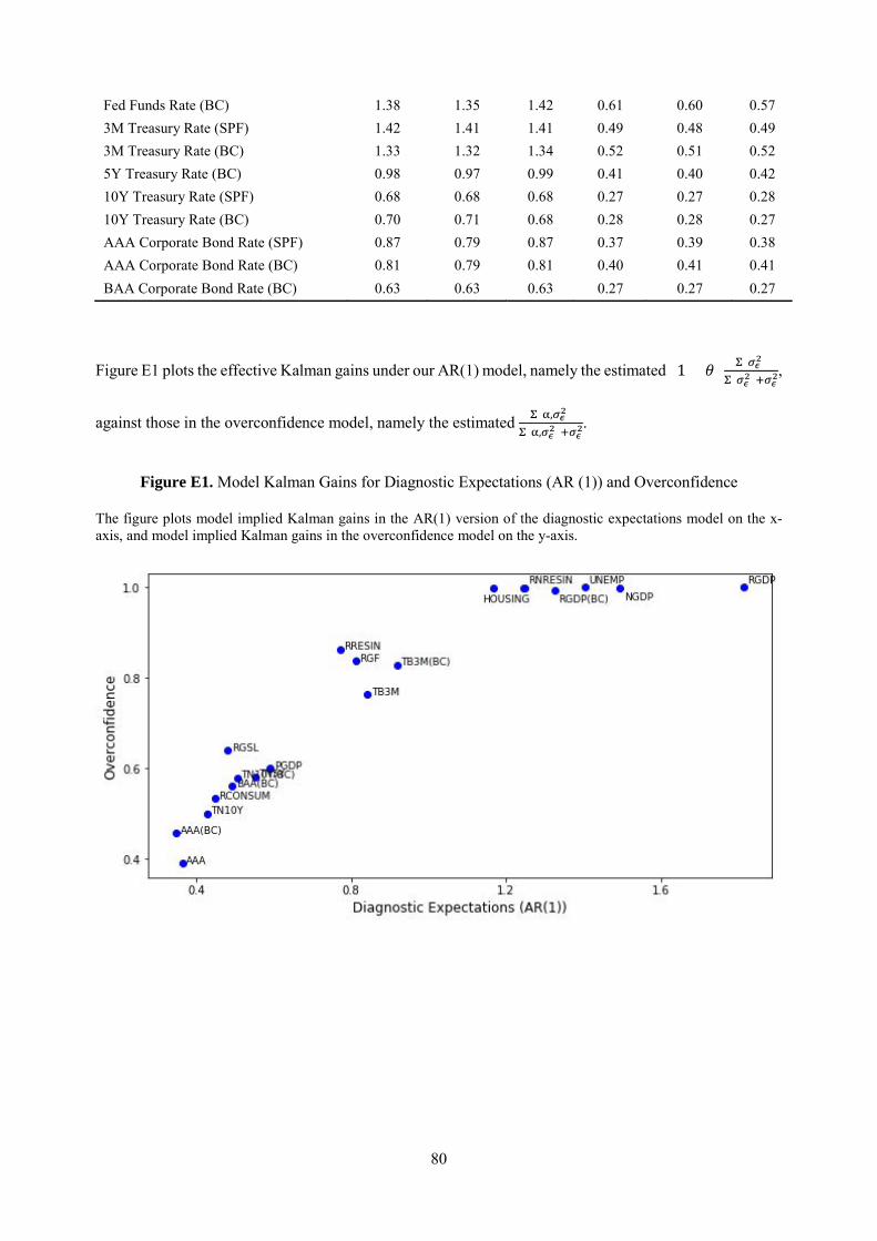
80

Figure E1 plots the effective Kalman gains under our AR(1) model, namely the estimated (1 + 𝜃𝜃) Σ(𝜎𝜎𝜖𝜖2)Σ(𝜎𝜎𝜖𝜖2)+𝜎𝜎𝜖𝜖2

,

against those in the overconfidence model, namely the estimated Σ(α,𝜎𝜎𝜖𝜖2)Σ(α,𝜎𝜎𝜖𝜖2)+𝜎𝜎𝜖𝜖2

.

Figure E1. Model Kalman Gains for Diagnostic Expectations (AR (1)) and Overconfidence

The figure plots model implied Kalman gains in the AR(1) version of the diagnostic expectations model on the x-axis, and model implied Kalman gains in the overconfidence model on the y-axis.

Fed Funds Rate (BC) 1.38 1.35 1.42 0.61 0.60 0.57 3M Treasury Rate (SPF) 1.42 1.41 1.41 0.49 0.48 0.49 3M Treasury Rate (BC) 1.33 1.32 1.34 0.52 0.51 0.52 5Y Treasury Rate (BC) 0.98 0.97 0.99 0.41 0.40 0.42 10Y Treasury Rate (SPF) 0.68 0.68 0.68 0.27 0.27 0.28 10Y Treasury Rate (BC) 0.70 0.71 0.68 0.28 0.28 0.27 AAA Corporate Bond Rate (SPF) 0.87 0.79 0.87 0.37 0.39 0.38 AAA Corporate Bond Rate (BC) 0.81 0.79 0.81 0.40 0.41 0.41 BAA Corporate Bond Rate (BC) 0.63 0.63 0.63 0.27 0.27 0.27