NBER WORKING PAPER SERIES

MARKET ACCESS ANDINTERNATIONAL COMPETITION:A SIMULATION STUDY OF

16K RANDOM ACCESS MEMORIES

Richard Baldwin

Paul R. Krugman

Working Paper No. 1936

NATIONAL BUREAU OF ECONOMIC RESEARCH1050 Massachusetts Avenue

Cambridge, MA 02138June 1986

This is a preliminary draft, not for quotation. Comments arewelcome. The research reported here is part of the NBER's researchprogram in International Studies. Any opinions expressed are thoseof the authors and not those of the National Bureau of EconomicResearch.

NBER Working Paper #1936June 1986

Market Access and International Competition:A Simulation Study of 16K Random Access Memories

ABSTRACT

This paper develops a model of international competition in an

oligopoly characterized by strong learning effects. The model is

quantified by calibrating its parameters to reproduce the US—Japanese

rivalry in 16K R.A.Ms from 1978-1983. We then ask the following question:

how much did the apparent closure of the Japanese market to imports

affect Japan's export performance? A simulation analysis suggests that a

protected home market was a crucial advantage to Japanese firms, which

would otherwise have been uncompetitive both at home and abroad. We

find, however, that Japan's home market protection nonetheless produced

more costs than benefits for Japan.

Richard BaldwinDepartment of EconomicsM.I.T.

Cambridge, MA 02139

Paul KrugmanDepartment of EconomicsM.I.T.Cambridge, MA 02139

The technology by which complex circuits can be etched and

printed onto a tiny silicon chip is a remarkable one. Until the late

1970s it was also a technology clearly dominated by the United States.

Thus it was a rude shock when Japanese competition became a serious

challenge to established US firms, and when Japan actually came to

dominate the manufacture of one important kind of chip, the Random

Access Memory (RAM). More perhaps than any other event, Japan's

breakthrough in RAMs has raised doubts about whether the traditional

American reliance on laissez—faire toward the commercialization of

technology is going to remain viable.

There are two main questions raised by shifting advantage in

semiconductor production. One is whether it matters who produces

semiconductors in general, or RAMs in particular. That is, does the

production of RAMs yield important country—specific external

economies? This is, of course, the $64K question. It is also an

extremely difficult question to answer. Externalities are inherently

hard to measure, because by definition they do not leave any trace in

market transactions. Ultimately the discussion of industrial policy

will have to come to grips with the assessment of externalities, but

for the time being we will shy away from that task.

In this paper we will instead focus on the other question. This

is where the source of the shift in advantage lies. Did Japan simply

acquire a comparative advantage through natural causes, or was

government targeting the key factor?

2

Although strong views can be found on both sides, this is also

not an easy question to answer. On one side, Japanese policy did not

involve large subsidies. The tools of policy were instead

encouragement with modest government support of a joint research

venture, the Very Large Scale Integration (VLSI) project, and tacit

encouragement of a closure of domestic markets to imports. Given that

Japan became a large scale exporter of chips, a conventional economic

analysis would suggest that government policy could not have mattered

very much.

Semiconductor manufacture, however, is not an industry where

conventional economic analysis can be expected to be a good guide. It

is an extraordinarily dynamic industry, where technological change

reduced the real price of a unit of computing capacity by 99 percent

from 1974 to 1984. This technological change did not fall as manna

from heaven; it was largely endogenous, the result of R&D and

learning—by-doing. As a result, competition was marked by dynamic

economies of scale that led to a fairly concentrated industry, at

least within the RAM market. So semiconductors is a dynamic oligopoly

rather than the static competitive market to which conventional

analysis applies.

Now it is possible to show that in a dynamic oligopoly the

policies followed by Japan could in principle have made a large

difference. In particular, a protected domestic market can serve as a

springboard for exports (Krugman 1984). The question, however, is how

3

important this effect has been. If the Japanese market had been as

open as US firms would have liked, would this have radically altered

the story, or would it have made only a small difference? There is no

way to answer this question without a quantitative model of the

competitive process.

The purpose of this paper is to provide a preliminary assessment

of the importance of market access in one important episode in the

history of semiconductor competition. This is the case of the 16K RAM,

the chip in which Japan first became a significant exporter. Our

question is whether the alleged closure of the Japanese market could

have been decisive in allowing Japan to sell not only at home but in

world markets as well. The method of analysis is the development of a

simulation model, derived from recent theoretical work, and

"calibrated" to actual data. The technique is in the same spirit as

the recent paper on the auto industry by Dixit (1985).

Obviously we are interested in the actual results of this

analysis. As we will see, the analysis suggests that privileged access

to the domestic market was in fact decisive in giving Japanese firms

the ability to compete in the world market as well. The analysis also

suggests, however, that this "success" was actually a net loss to the

Japanese economy. Finally, the attempt to Construct a simulation model

here raises many difficult issues, to such an extent that the results

must be treated quite cautiously.

4

The modelling endeavor has a secondary purpose, however, which

may be more important than the first. This is to conduct a trial run

of the application of new trade theories to real data. It is our view

that RAMs are a uniquely rewarding subject for such a trial run. On

one hand, the product is well defined: RAMs are a commodity, in the

sense that RAils from different firms are near—perfect substitutes and

can in fact be mixed in the same device. Indeed, successive

generations of RAMs are still good substitutes —— a 16K RAM is pretty

close in its use to four 4K RAMs, and so on. On the other hand, the

dynamic factors that new theory emphasizes are present in RAMs to an

almost incredible degree. The pace of technological change in RAMs is

so rapid that other factors can be neglected, in much the same way

that non—monetary factors can be neglected in studying hyperinflation.

This paper is in five parts. The first part provides background

on the industry. The second part develops the theoretical model

underlying the simulation. In the third part we explain how the model

was "calibrated" to the data. In the fourth part we describe and

discuss simulations of the industry under alternative policies.

Finally, the paper concludes with a discussion of the significance of

the results and directions for further research.

THE RANDOM ACCESS MEMORY MARKET

5

Techrio logy and the_growth of the industry

So—called dynamic random access memories are a particular

general—purpose kind of semiconductor chip. What a RAM does is to

store information in digital form, in such a way as to allow that

information to be altered (hence 'dynamic") and read in any desired

order (hence 'random access"). The technique of production for 16K

RAMs involved the etching of circuits on silicon chips by a

combination of photographic techniques and chemical baths, followed by

baking. The advantage of this method of manufacture, in addition to

the microscopic scale on which components are fabricated, is that in

effect thousands of electronic devices are manufactured together with

the wires that connect them, all in a single step. The disadvantage,

if there is one, is that the process is a very sensitive one. If a

chip is to work, everything —— temperature, timing, density of

solutions, vibration levels, dust —- must be precisely controlled.

Getting these details right is as much a matter of trial and error as

it is a science.

The sensitivity of the manufacturing process gives rise to a very,

distinctive form of learning-by-doing. Suppose that a semiconductor

chip has been designed and the manufacturing process worked out. Even

so, when production begins the yield of usable chips will ordinarily

be very low. That is, chips will be produced, but most of them ——

often 95 percent —— will not work, because in some subtle way the

6

conditions for production were not quite right. Thus the manufacturing

process is in large part a matter of experimenting with details over

time. As the details are gotten right, the yield rises sharply. Even

at the end, however, many chips still fail to work.

Technological progress in the manufacture of chips has had a more

or less regular rhythm in which fundamental improvements alternate

with learning—by—doing within a given framework. In the case of RAMs

the fundamental innovations have involved packing ever more components

onto a chip, through the use of more sophisticated methods of etching

the circuits. Given the binary nature of everything in this industry,

each such leap forward has involved doubling the previous density;

since chips are two—dimensional, each such doubling of density

quadruples the number of components. Thus the successive generations

of RAMs have been the 4K (4x210), the 16K, the 64K, and the 256K.

Basically a 16K chip does four times as much as a 4K, and given time

costs not much more to produce, so the succession of generations

creates a true product cycle in which each generation becomes more or

less throroughly replaced by the next.

Table 1 shows how the sucessive generations of RAMs have entered

the market, and how the price has fallen. To interpret the data, bear

in mind that one unit of each generation of RAM is roughly equivalent

to four units of the previous generation. The pattern of product

cycles then becomes clear. The effective output of 16K RAMs was

already larger than that of 4Ks in 1978, and the effective price was

7

clearly lower by 1979. The 16K RAM was in its turn overtaken in output

in 1981, in price in 1982. As of the time of writing the 64K has not

yet been overtaken by 256K RAMs. Missing from the table, as well, is a

collapse in RAM prices during 1985, to levels as little as a tenth of

those of a year earlier.

From an economists point of view, the most important question

about a technology is not how it works but how it is handled by a

market system. This boils down largely to the questions of

appropriability and externality. Can the firm that develops a

technological improvement keep others from imitating it long enough to

reap the rewards of its cleverness? Do others gain from a firmts

innovations (other than from its improved product or reduced prices)?

When we examine international competition, we also want to know

whether external benefits, to the extent that they are generated, are

national or international in scope.

From the nature of what is being learned, there seem to be clear

differences between the two kinds of technological progress in the

semiconductor industry. When a new generation of chips is introduced,

the knowledge involved seems to be of kinds that are relatively hard

to maintain as private property. Basic techniques of manufacture are

hard to keep secret, and in any case respond to current trends in

science and "metatechno].ogy'. Thus everyone knew in the late 1970s

that a 64K RAM was possible, and roughly speaking how it was going to

be done. Furthermore, even the details of chip design are essentially

8

impossible to disguise: firms can and do make and enlarge photographs

of rivals' chips to see how their circuits are laid out. Also, the

ability of firms to learn from each other is not noticeably restricted

by national boundaries.

The details of manufacture, as learned over time in the process

of gaining experience, are by contrast highly appropriable. The facts

learned pertain to highly specific circumstances, and are indeed

sometimes plant— as well as firm—specific. Unlike the design of the

chips, the details of production are not evident in the final product.

Thus the knowlege gained from learning-by-doing in this case is a

model of a technology that poses few appropriability problems.

It seems, then, that the basic innovations involved in passing

from one generation to the next in RAMs are relatively hard to

appropriate, while those involved in getting the technology to work

within a generation are relatively easy to appropriate. This

observation will be the basis of the key untrue assumption that we

will make in implementing our simulation analysis. We will treat

product cycles —— the displacement of one generation by the next,

better one —— as completely exogenous. This will allow us to focus

entirely on the Competition within the cycle, in which technological

progress takes place by learning. It will also allow us to put time

bounds on this competition: a single product cycle becomes the natural

unit of analysis.

9

Like any convenient assumption, this one does violence to

reality. It is at least possible that the assumptions we make are in

fact missing the key point of Competition in this industry. For now,

however, let us make our simplification and leave the critical

discussion to the end of the paper.

Market structure and trade policy

Some fourteen firms produced 16K random access memories for the

commercial market during the period 1977-83. Table 2 shows the average

shares of these firms in world production during the period. Taken as

a whole, the industry was not exceptionally concentrated, though far

from competitive: the Herfindahl index for all firms, taking the

average over the period, was only 0.099. This overstates the effective

degree of competition, however, for two main reasons. First, some of

the firms producing small quantities were probably producing

specialized products in short production runs, and thus were really

not producing the same commodity as the rest. Second, there was, as we

will see shortly, a good deal of market segmentation between the US

and Japan, so that each market was substantially more oligopolized

than the figures suggest. Nonetheless, when we create a stylized

version of the market for simulation purposes, we will want to make

sure that the degree of competition is roughly consistent with this

data. As it turns out, we will develop a model in which the baseline

10

case contains six symmetric US firms and three symmetric Japanese

firms, which does not seem too far off.

Another feature of the semiconductor industry's market structure

does not show in the table. This is the contrast between the nature of

the US firms and their Japanese rivals. The major US chip

manufacturers shown here are primarily chip producers. (There is also

"captive" US production by such firms as IBM and ATT, but during the

period we are considering little of this production found its way to

the open or "merchant" market). The Japanese firms, by contrast, are

also substantial consumers of chips in their other operations. The

Japanese firms are not, however, vertically integrated in the usual

sense. Each buys most of its chips from other firms, while in turn

selling most of its chip output to outside customers. There have been

repeated accusations, however, that the major suppliers and buyers of

Japanese semiconductor production —— who are the same firms —— collude

to form a closed market and exclude foreign sources.

The claim that the Japanese market was effectively closed rests

on this difference in market structure. US firms argued that the buy-

Japanese policy of the major firms was tacitly and perhaps even

explicitly encouraged by the government, so that even in the absence

of any formal tariffs or quotas Japan was able to use a strategy of

infant—industry protection to establish itself. It is beyond our

ability to assess such claims, or to determine how important the

government of Japan as opposed to its social structure was in closing

11

the market to foreigners. There is, however, circumstantial evidence

of a less than open market. The evidence is that of market shares.

Consider Table 3 (which is subject to some problems; see the

appendix). We see that US firms dominated both their own home market

and third—country markets, primarily in Europe. Yet they had a small

share in Japan, probably again in specialized types of RAMs rather

than the basic commodity product. Transport costs for RAMs are small;

they are, as we have stressed, commodity—like in their

interchangeability. So the disparity in market shares suggests that

some form of market closure was in fact happening.

Here is where economic analysis comes in. We know that in an

industry characterized by strong learning effects, as we have argued

is the case here, protection of the home market can have a kind of

multiplier effect. Privileged access to one market can give firms the

assurance of moving further down their learning curves and thus

encourage them to price aggressively in other markets as well. Our

next task will be to develop a simulation model which can be used to

ask how important this effect could have been in the case of RAMs.

A THEORETICAL MODEL OF COMPETITION IN RAMS

Learning, capacity, and prices

12

We have argued that a useful approximation to the nature of

technological change in RAMs is to divide it into two kinds. Major

technological change, the shift to a new capacity of chip, can be

provisionally treated as an exogenous event, external to firms. Within

each product cycle, however, increased yield of chips can be thought

of as the endogenous result of learning—by—doing, internal to firms.

This distinction makes it seem natural to analyze competition

within each product cycle using the learning curve models of Spence

(1981) and of Fudenberg and Tirole (1983). This was in fact our

initial approach to the problem. We found, however, that while these

models are in the right spirit, they have difficulty coping with a

crucial aspect of the data: the pace at which output rises and prices

fall within each product cycle. This forced us to modify the analysis.

To understand this problem, consider Spence's simplest model ——

which is the one we would have liked to use. He assumes that firms

face a product cycle of known length, short enough so that discounting

can be ignored. At each point in this product cycle, a firm's marginal

cost is a decreasing function of its cumulative output to date. (These

are not bad approximations to the situation in RAMs). He also assumes

that firms follow "open loop" strategies, ruling out the possibility

of strategic moves to influence rivals' later behavior.

Now the result of these assumptions is gratifyingly simple.

Essentially the dynamic problem of the firm collapses into a static

13

one. The true marginal cost of a firm at any point is its direct

marginal production cost, less the contribution of an additional unit

of current output to reducing later costs. As the product cycle

proceeds, the first term declines as experience is gained, but so does

the second, because there is less future production to which cost

savings can be applied. What Spence showed was that these two terms

decline at exactly the same rate: true marginal cost remains constant

over time. At the end of the product cycle, of course, the second term

vanishes. Thus throughout the product cycle the marginal cost that is

set equal to marginal revenue is simply the marginal cost of

production of the last unit that will be produced.

What is wrong with this analysis? Suppose that demand were

constant. Then Spence's model would imply that each firm has constant

marginal cost, and thus that both prices and output would remain

constant over the cycle. This is clearly massively inconsistent with

the data in Table 1.

How can we resolve this conflict? One answer would be to adopt a

more sophisticated learning curve model. We could, for instance,

introduce discounting; this would, as Fudenberg and Tirole have shown,

lead to a declining rather than a constant price. It is hard to

believe, however, that this could explain a 90 percent decline over

four years. Alternatively, we could follow Fudenberg and Tirole by

letting firms follow closed loop strategies and thus allowing for

strategic moves. If anything, however, this would seem to lead to

14

rising prices, because firms would try to aggressively establish an

advantage in the first part of the product cycle, then reap the

rewards later. Either of these solutions, furthermore, has the problem

of spoiling the simplicity of Spence's formulation. The firints dynamic

problem can no longer be collapsed into a static one. This may be the

truth, but we are looking for something that can be made operational,

and it would be very desirable to have a simpler model.

A clue to the resolution of this problem may be found by

considering another disconcerting feature of Spence's model. Suppose

again that demand is constant, and that therefore production remains

constant. It follows, given rising efficiency, that the quantity of

resources devoted to production is actually at its maximum at the

beginning of the cycle, and declines steadily from then on. I.e.,

firms build plants, then gradually dismantle them as they become more

efficient! This seems clearly implausible. Surely a better formulation

is to suppose that resources, once committed to production, stay there

throughout the product cycle. If this is the case, however, we can no

longer treat marginal cost in the same way. Resources committed to

production —- call them "capacity" —— are a sunk cost once they are in

place.

The view that productive resources in RAM production constitute a

sunk cost, and that ex—post supply is inelastic, gains further

strength from recent gyrations in prices. In the year and a half

before this paper was written, RAM prices first fell by a factor of

15

ten, then tripled. These fluctuations could not happen if firms were

able to move resources freely in and out of the sector.

We have therefore adopted a model similar in spirit to the

learning curve approach, but different in its dynamic implications.

This is the "yield curve" model of production. At the beginning of the

product cycle firms choose a level of capacity that they commit to

production throughout the cycle. The output from any given level of

capacity rises through time, as experience is gained. Since capacity

is a sunk cost, firms sell whatever they produce, no matter what the

price: having chosen capacity, firms must let the chips fall where

they may. Since output rises with experience, price falls over time.

This is the general idea; let us now turn to the specifics.

The Yield Curve Model of Production

Consider a firm that at the start of a product cycle commits some

amount of resources to production. We will define one unit of capacity

as the resources needed to produce one "batch" per unit of time (see

below); let K be the capacity in which a firm invests.

Now we will suppose that production takes the form of "batches":

each period, one unit of capacity can be used to engrave and bake one

batch of semiconductor chips. Thus the firm produces batches at a

constant rate K throughout the cycle, and the total number of batches

produced after t periods has passed is Kt.

16

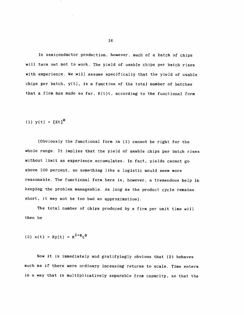
In semiconductor production, however, much of a batch of chips

will turn out not to work. The yield of usable chips per batch rises

with experience. We will assume specifically that the yield of usable

chips per batch, y(t), is a function of the total number of batches

that a firm has made so far, K(t)t, according to the functional form

(1) y(t) = [K]e

(Obviously the functional form in (1) cannot be right for the

whole range. It implies that the yield of usable chips per batch rises

without limit as experience accumulates. In fact, yields cannot go

above 100 percent, so something like a logistic would seem more

reasonable. The functional form here is, however, a tremendous help in

keeping the problem manageable. As long as the product cycle remains

short, it may not be too bad an approximation).

The total number of chips produced by a firm per unit time will

then be

(2) x(t) = Ky(t) = Kl$t0

Now it is immediately and gratifyingly obvious that (2) behaves

much as if there were ordinary inceasing returns to scale. Time enters

in a way that is multiplicatively separable from capacity, so that the

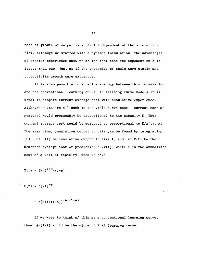
17

rate of growth of output is in fact independent of the size of the

firm. Although we started with a dynamic formulation, the advantages

of greater experience show up as the fact that the exponent on K is

larger than one, just as if the economies of scale were static and

productivity growth were exogenous.

It is also possible to show the analogy between this formulation

and the conventional learning curve. In learning curve models it is

usual to compare current average cost with cumulative experience.

Although costs are all sunk in the yield curve model, current cost as

measured would presumably be proportional to the capacity K. Thus

current average cost would be measured as proportional to K/x(t). At

the same time, cumulative output to date can be found by integrating

(2). Let X(t) be cumulative output to time t, and let C(t) be the

measured average cost of production cK/x(t), where c is the annualized

cost of a unit of capacity. Then we have

X(t) = (K)l--e/(l+O)

C(t) = c(Kt)

= c[X(t)(l+e)J_8/+0)

If we were to think of this as a conventional learning curve,

then, 01(1+0) would be the slope of that learning curve.

18

The close parallels between our formulation and both static

economies of scale, on one side, and the learning curve, on the other,

are very helpful. Usually studies of technological change in

semiconductors have been framed in terms of learning curves; what we

can do is reinterpret the results of those studies in terms of a yield

curve, transforming estimates of the learning curve elasticity to

derive estimates of 8. At the same time, the parallel with static

economies of scale suggests a solution technique for our model, when

it is fully specified: collapse it into an equivalent static model,

and solve that model instead. We need to specify the demand side to

show that in fact such a procedure is valid, but this will in the end

be the technique we use.

A final point about the assumed technology. The reason for

assuming the yield curve as opposed to the learning curve model is

that it implies growing output over the product cycle. Can we say

anything more than this? The answer is that the specific formulation

adopted here implies also that output grows at a declining rate. By

taking logs and differentiating (2), we find that the rate of growth

of output will decline according to the relationship

(3) (dx(t)/dt)/x(t) e/t

The prediction of a declining rate of growth in output over the

product cycle is borne out, except for a slight reversal at one point,

by the data in Table 1.

19

Demand and trade

Turning now to the demand side, we suppose that there are two

markets, the US and Japan. We denote Japanese variables with an

asterisk, while leaving US. variables unstarred. In each market there

is a constant elasticity demand curve for output, which we write in

inverse form as

(4) p = AQ

(5) P =

We thus assume that the elasticity of demand, 1/a, is the same in both

markets.

Firms will assumed to be located in one market or the other, and

to be able to ship to the other market only by incurring an additional

transport cost. Transport costs will be of the "iceberg" variety, with

only a fraction 1/(l÷d) of any quantity shipped arriving.

The problem of firms has two parts. First, they must decide on a

capacity level. This fixes the path of their output through the

product cycle. Second, at each point in time they must decide how much

to sell in each market. Let us for the moment take the capacity choice

as given, and focus only on the determination of the division of

output.

20

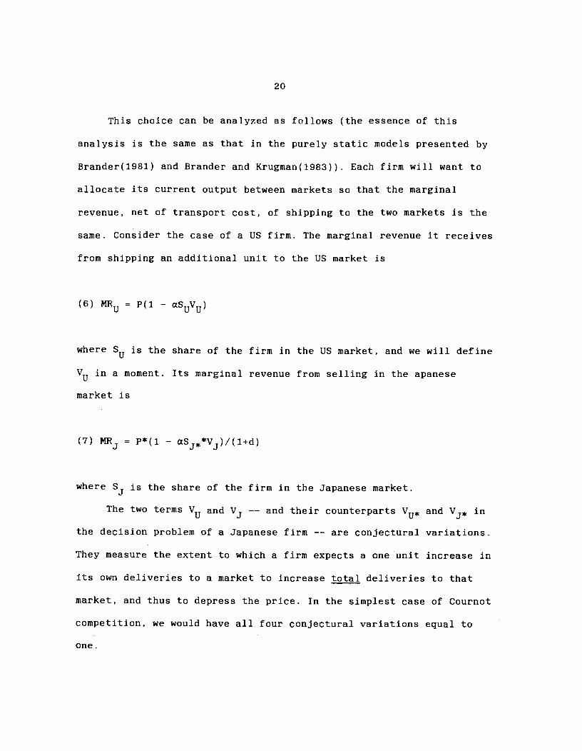
This choice can be analyzed as follows (the essence of this

analysis is the same as that in the purely static models presented by

Brander(1981) and Brander and Krugman(1983)). Each firm will want to

allocate its current output between markets so that the marginal

revenue, net of transport cost, of shipping to the two markets is the

same. Consider the case of a US firm. The marginal revenue it receives

from shipping an additional unit to the US market is

(6) = P(l - aSV)

where S is the share of the firm in the US market, and we will define

VU in a moment. Its marginal revenue from selling in the apanese

market is

(7) ffi = p*(l —

where S is the share of the firm in the Japanese market.

The two terms V and V —- and their counterparts and V3, in

the decision problem of a Japanese firm —— are conjectural variations.

They measure the extent to which a firm expects a one unit increase in

its own deliveries to a market to increase total deliveries to that

market, and thus to depress the price. In the simplest case of Cournot

Competition, we would have all four conjectural variations equal to

one.

21

The use of a conjectural variations approach in modelling

oligopoly is not a favored one. Many authors have pointed out the

shaky logical foundations of the approach, and to use it in an

empirical application adds an uncomfortable element of ad—hockery. We

introduce these terms now because we have found that we need them;

indeed, it will become immediately apparent as soon as we discuss

entry that to reconcile the industry's structure with its technology

we must abandon the hypothesis of Cournot competition. Whether there

are alternatives to the conjectural variation approach is a question

we will return to at the end of the paper.

Suppose that we suppress our doubts, and accept the conjectural

variations approach. Then we can notice the following point. Suppose

that for some P,P, S and S the first—order condition MRu = MR is

satisfied. Then the condition will continue to be satisfied with the

same S and S even for different prices, as long as P/Ps remains the

same.

What this means is that if all firms grow at the same rate, so

that it is feasible for them to maintain constant market shares, and

if prices fall at the same rate in both markets, the optimal behavior

will in fact be to maintain constancy of market shares. Fortunately,

our assumptions on the yield curve insure that all firms will indeed

grow at the same rate. Furthermore, if firms continue to divide their

output in the same proportions between the two markets, the fact that

all firms grow at the same rate and that the elasticity of demand is

22

assumed constant insures that prices in the two markets will indeed

fall at the same rate. So we have demonstrated that given the initial

capacity decisions of the firms, the subsequent equilibrium in the

product cycle is a sort of balanced growth in which market shares do

not change but output steadily rises and prices steadily fall.

We note finally that in principle this equilibrium may be one in

which there is two—way trade in the same product. Firms with a small

market share (or a low conjectural variation) in the foreign market

may choose to 'dump" goods in that market, even though the price net

of transport and tariff costs is less than at home. Since this may be

true of firms in each country, the result can be two—way trade based

on reciprocal dumping.

So far we have discussed equilibrium given the number of firms

and their capacity choices; our final steps are to consider capacity

choice and entry.

Capacity choice

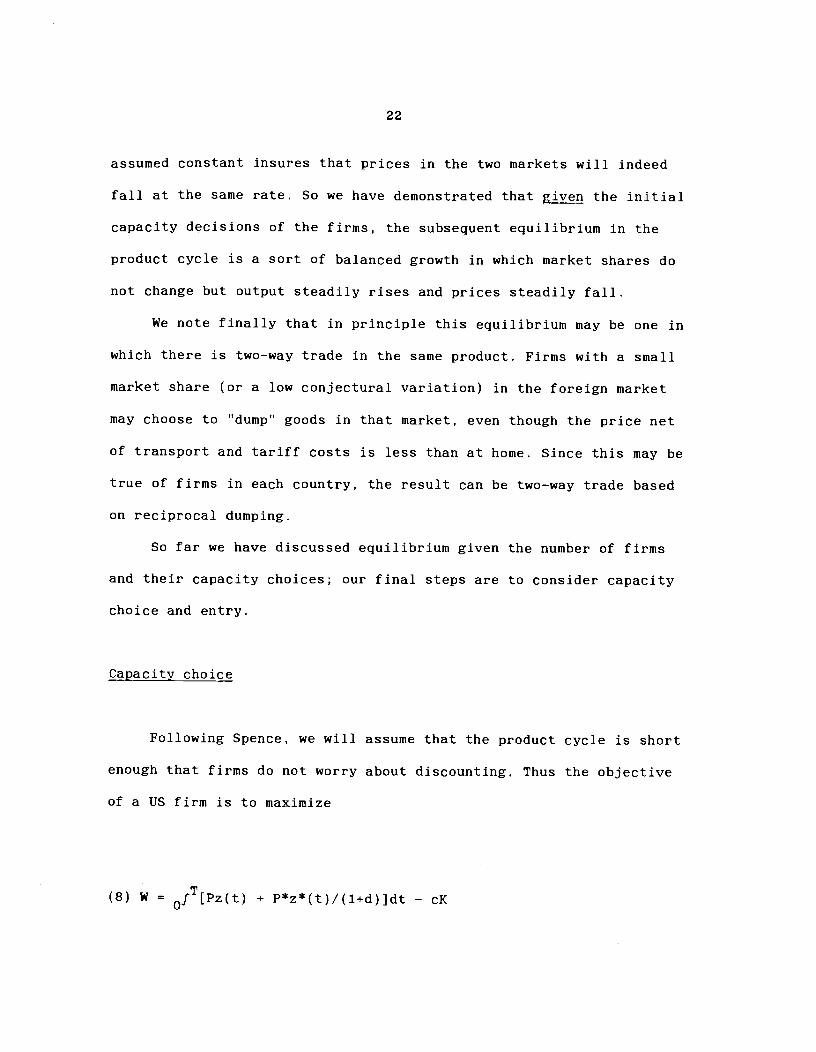
Following Spence, we will assume that the product cycle is short

enough that firms do not worry about discounting. Thus the objective

of a US firm is to maximize

(8) w = fT[Pz(t) + p*z*(t)/(1+d)]dt — cK

23

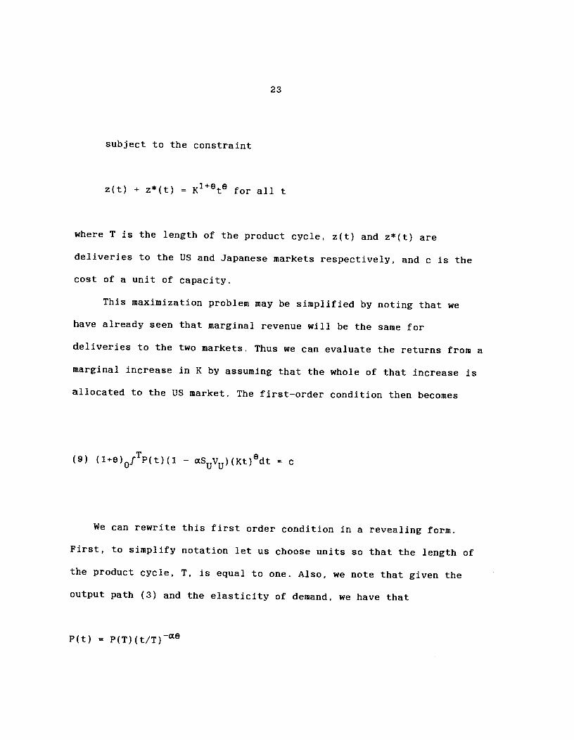
subject to the constraint

z(t) + z*(t) = K18t0 for all t

where T is the length of the product cycle, z(t) and z*(t) are

deliveries to the US and Japanese markets respectively, and c is the

cost of a unit of capacity.

This maximization problem may be simplified by noting that we

have already seen that marginal revenue will be the same for

deliveries to the two markets. Thus we can evaluate the returns from a

marginal increase in K by assuming that the whole of that increase is

allocated to the US market. The first—order condition then becomes

(9) (l+e)0fTp(t)(j. — aSV) (1(t) dt = c

We can rewrite this first order condition in a revealing form.

First, to simplify notation let us choose units so that the length of

the product cycle, T, is equal to one. Also, we note that given the

output path (3) and the elasticity of demand, we have that

P(t) = P(T)(t/T)0

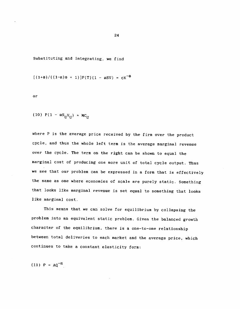
24

Substituting and integrating, we find

{(1+e)/((1—a)e + 1)JP(T)(1 — aSV) = CK0

or

(10) P(l - aSuvu) MCu

where P is the average price received by the firm over the product

the whole left term is the average marginal revenue

The term on the right can be shown to equal the

producing one more unit of total cycle output. Thus

problem can be expressed in a form that is effectively

where economies of scale are purely static. Something

marginal revenue is set equal to something that looks

that we can solve for equilibrium by collapsing the

problem into an equivalent static problem. Given the balanced growth

character of the equilibrium, there is a one-to—one relationship

between total deliveries to each market and the average price, which

continues to take a constant elasticity form:

(11) p = AQ

cycle, and thus

over the cycle.

marginal cost of

we see that our

the same as one

that looks like

like marginal cost

This means

25

And we can write an average cost function for cumulative output which

takes the form

(12) C = cx')A model of the form (iO)—(12) may be solved using methods

described in Brander and Krugman(l983) and Krugman(1984). For any

given marginal costs we can solve for equilibrium prices and market

shares. From prices we can determine total sales, and using market

shares use this to find output per firm. This output, however, implies

a marginal cost. A full equilibrium is a fixed point where the

marginal Costs assumed at the beginning are the same as those implied

at the end. In practice such an equilibrium can easily be calculated

using an iterative procedure. We make a guess at the marginal costs,

solve for output, use this to recompute the marginal costs, and

continue until convergence.

Once we have solved this collapsed problem, we can then solve for

the implied capacity choices and the whole time path of output and

prices.

Entry

26

Finally, we turn to the problem of entry. Here we assume that

there are many potential entrants with the same costs, and that all

potential entrants have perfect foresight about the post—entry

equilibrium. An equilibrium with entry must then satisfy two criteria:

it must yield non—negative profits for all those firms who do enter,

but any additional firm that might enter would face losses. If we

could ignore integer constraints this would imply a zero-profit

equilibrium. In practice this will not be quite the case. However, as

we will see, our estimates of profits turn out to be quite small.

An important point about the relationship between entry and

conjectural variations should be noted. This is that the conjectural

variations must be high —— that is, post—entry firms had better not be

too competitive —— if there are strong increases in yield. To see

this, consider a single market with elasticity of demand 1/a and yield

curve parameter e, where all firms are the same. Then the number of

firms that can earn zero profits can be shown to be a(l+e)V/e, where V

is the conjectural variation. For the estimates of a and e that we

will be using, this turns out to be l.98V. That is, with Cournot

behavior only 2 firms could earn zero profits. Not surprisingly, in

order to rationalize the existence of the six large US firms that

actually competed, and who furthermore faced some foreign competition,

we end up needing to postulate behavior a good deal less competitive

than Cournot.

27

We have now described a theoretical model of competition in an

industry that we hope Captures some of the essentials of the Random

Access Memory market. Our next step is to try to make this model

operational using realistic numbers.

CALIBRATING THE MODEL

Our theoretical model of the random access memory market is

recognizably one in which protection of the domestic market will in

effect push a firm down its marginal cost curve and lead to a larger

share of the export market as well. What we want to do, however, is to

quantify this effect. To do this, we need to choose realistic

parameter values. What we did was to take outside estimates for some

of the parameters, then use data on the industry to calibrate the

model to fix the remaining parameters.

Parameters from outside estimates

The parameters for which we took numbers directly from other

sources were the elasticity of demand, a; the elasticity of the yield

curve, e; and the transport cost d.

Finan and Amundsen (1985) estimates demand elasticity at 1.8 for

the US market. In fact we can confirm that this must be at least

28

approximately right by comparing the fall in prices and the rise in

quantity over the period 1978—1981, i.e., over the period when 16K

RAMs were the dominant memory chip. Prices fell by a logarithmic 142

percent over that period, while sales rose by 233 percent, 1.6 times

as much, despite a recession and high interest rates that depressed

investment. In general, it is apparent that the elasticity of demand

for semiconductor memories must be more than one but not too much

more, given that the price per bit has fallen 99 percent in real terms

over the past decade. If demand were inelastic, the industry would

have shrunk away; if it were very elastic, we would be having chips

with everything by now.

The elasticity of the yield curve can, as we noted in our earlier

discussion, be derived from the elasticity of the associated learning

curve. Discussions of learning curves in general often offer numbers

in the 0.2—0.3 range. An Office of Technology Assessment study (Office

of Technology Assessment, 1983) estimated the slope of the learning

curve for semiconductors at 0.28. Converted to yield curve form, this

implies 0 = 0.3889.

Finally, there is general agreement that costs of transporting

semiconductors internationally are low, as one would expect given the

high ratio of value to weight or bulk. We follow Finants estimate of

d=O. 05.

Costs

29

The data in Tables 2 and 3 show fourteen firms in three markets.

If we were to try to represent the complete structure of the industry,

we would need to specify 14 cost functions and 42 conjectural

variations parameters. Instead, we have stylized the market in such a

way as to need to specify only two cost parameters and four

conjectural variations.

The less important step in this stylization is the consolidation

of the US and ROW markets into a single market. This may be justified

on the grounds that transport costs are small, and the crucial issue

is the alleged closure of the Japanese market. Also, as our data

suggests, the market share of US firms in the US and ROW markets is

fairly similar.

The more important step is the representation of the US and

Japanese industries as a group of symmetrical representative firms.

There are many objections to this procedure. The essential problem is

that the size distribution of firms presumably has some meaning, and

to collapse it in this way means that we are neglecting potentially

important aspects of reality. As with the other problematic

assumptions in this paper, this should be viewed as a simplification

that we hope is not crucial.

In Table 2 we noted that there were nine firms with market shares

over five percent: six US and three Japanese. We represent the

industry by treating it as if these were the only firms, and as if all

30

firms from each country were the same. Thus our model industry

consists of six equal—cost US firms, which share the entire US market

share, and three equal—cost Japanese firms, which do the same for

Japan's market shares.

We do not have direct data on costs. Instead, we attempt to infer

costs by assuming that in the actual case firms earned precisely zero

profits. As we know, because of integer constraints this need not have

been the case. It should have been close, however, and it allows us to

use price and output data to infer costs.

First, we have data on prices. This data shows that from 1978—

1983 the average price of a 16K RAM was identical in the two markets,

at 1.47 dollars. There is reason to suspect this data, since the

Japanese had been threatened with an anti—dumping action and the

structure of the Japanese industry may have made it easy for effective

prices to differ from those posted. Lacking any information on this,

however, we will go with the official data.

Next, we use our stylized industry structure to calculate the per

firm sales in each market. These are shown in the first part of Table

4. Given this information, we can net out transport costs on foreign

sales to calculate the average revenue of a representative firm of

each type: that is,

IT[p(t)z(t) + p*(t)(z*(t))/(1-,d)]dt/ 0fT[z(t) + z*(t)]dt

31

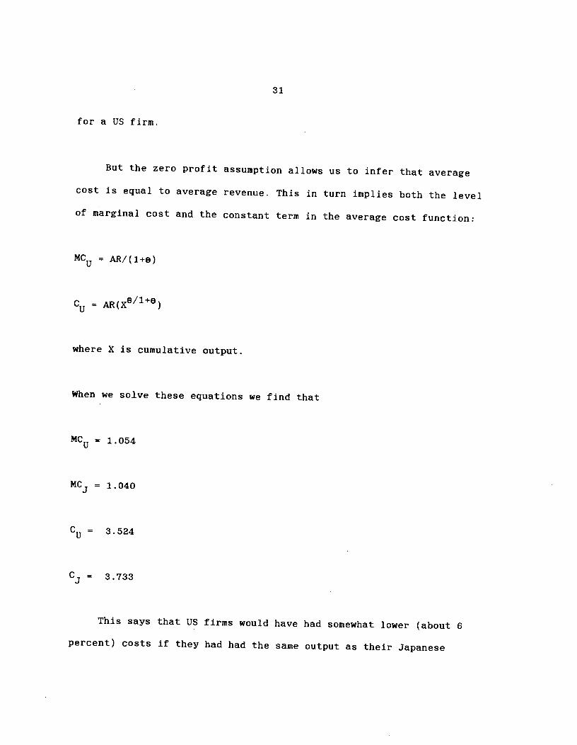
for a US firm.

But the zero profit assumption allows us to infer that average

cost is equal to average revenue. This in turn implies both the level

of marginal cost and the constant term in the average cost function:

MCu AR/(1+)

CU= AR(Xe/l÷e)

where X is cumulative output.

When we solve these equations we find that

MCu = 1.054

MC3 = 1.040

CU = 3.524

C3 = 3733

This says that US firms would have had somewhat lower (about 6

percent) Costs if they had had the same output as their Japanese

32

rivals, but that Japanese firms, thanks to larger scale, ended up with

very slightly lower marginal costs.

This result confirms what industry experts have claimed in a

qualitative sense about the industry. Most estimates based on direct

observation have given US firms a larger inherent cost advantage ——

Finan and Amundsen (1985) suggests 10—15 percent. Given the roundabout

nature of our method, and the problems of some of our data, we would

not quarrel with this.

One might wonder about the coincidence that costs in the two

countries appear to be so close. Is there something about our method

that forces this? The answer, we believe, is that this is a result of

our method of selecting an industry to study. The 16K RAN was the

first semiconductor in which Japan became an exporter on a large

scale. Not surprisingly, it is one in which costs were close. Had we

done the 4K RAM, in which Japanese firms sold only to a protected

domestic market, or the 64K RAN, in which they came to be the dominant

producers, we would presumably have found quite different answers.

Conjectural variations

Our next step is to calculate conjectural variations parameters.

We begin with per firm market shares: these are shown in the second

part of Table 4.

33

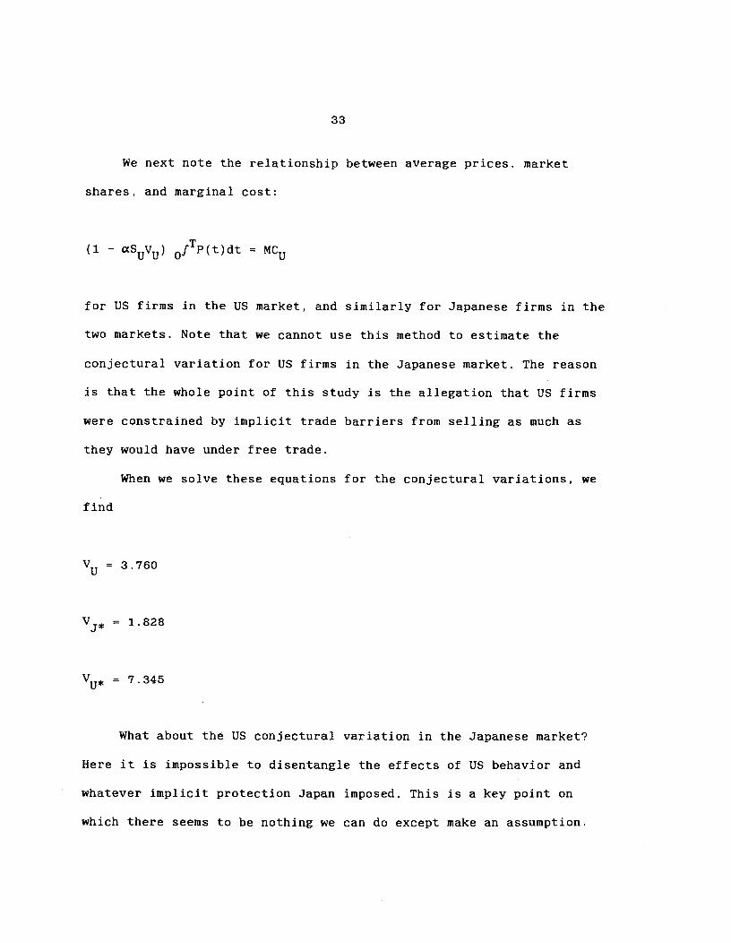
We next note the relationship between average prices, market

shares, and marginal cost:

(1 - SuVu) fTp(t)dt = Mcu

for US firms in the US market, and similarly for Japanese firms in the

two markets. Note that we cannot use this method to estimate the

conjectural variation for US firms in the Japanese market. The reason

is that the whole point of this study is the allegation that US firms

were constrained by implicit trade barriers from selling as much as

they would have under free trade.

When we solve these equations for the conjectural variations, we

find

VU = 3.760

V, = 1.828

= 7•345

What about the US conjectural variation in the Japanese market?

Here it is impossible to disentangle the effects of US behavior and

whatever implicit protection Japan imposed. This is a key point on

which there seems to be nothing we can do except make an assumption.

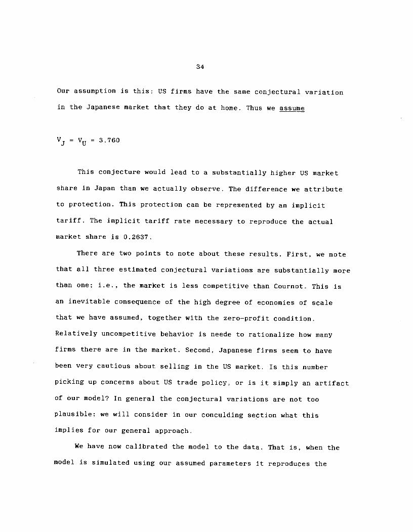
34

Our assumption is this: US firms have the same conjectural variation

in the Japanese market that they do at home. Thus we assume

=VU

= 3.760

This conjecture would lead to a substantially higher US market

share in Japan than we actually observe. The difference we attribute

to protection. This protection can be represented by an implicit

tariff. The implicit tariff rate necessary to reproduce the actual

market share is 0.2637.

There are two points to note about these results. First, we note

that all three estimated conjectural variations are substantially more

than one; i.e., the market is less competitive than Cournot. This is

an inevitable consequence of the high degree of economies of scale

that we have assumed, together with the zero—profit condition.

Relatively uncompetitive behavior is neede to rationalize how many

firms there are in the market. Second, Japanese firms seem to have

been very cautious about selling in the US market. Is this number

picking up concerns about US trade policy, or is it simply an artifact

of our model? In general the conjectural variations are not too

plausible; we will consider in our conculding section what this

implies for our general approach.

We have now calibrated the model to the data. That is, when the

model is simulated using our assumed parameters it reproduces the

35

actual prices, outputs, and market shares of the 16K RAM product

cycle. We summarize this baseline case in Table 5. Our next step is to

ask how the results change under alternative policies.

EFFECTS OF ALTERNATIVE POLICIES

We consider two alternative policies. First is free trade,

represented in our model by a removal of the implicit tariff on US

sales to Japan. Second is a trade war, in which both countries block

imports. The effects of the two policies are shown next to the

baseline case in Table 5.

It is important to note the underlying assumptions behind these

calculations. In each case all parameters are assumed constant, except

for the implicit tariff on US exports to Japan. In particular, the

conjectural variations are assumed to remain unchanged. This is not a

particularly satisfactory assumption, but of course if we allow these

parameters to change anything can happen.

To solve the model in each case, we followed a two—stage

procedure. First, we took the initial number of firms and iterated on

marginal cost to get the equilibrium. Then we searched across a grid

of numbers of Japanese and US firms to find an entry equilibrium.

Free trade

36

Our first policy experiment goes to the heart of the debate over

Japanese trade policy. We ask what would have happened if the Japanese

market had been open. This is done by removing the implicit tariff on

Us exports to Japan.

The results, reported in the second column of Table 5, are quite

striking. According to our model, in the absence of protection, the

Japanese firms that were net exporters in the baseline case do not

even enter; only US firms remain in the field. The reason is a sort

circular causation typical in models with scale economies. Japanese

firms, deprived of their safe haven in the domestic market, would have

smaller cumulative output even with constant marginal cost. The

smaller output, however, means a higher marginal cost. This implies

still smaller output, which implies still higher marginal cost, and so

on. In the end, no Japanese firms find it profitable to enter.

The exit of the Japanese firms, and the new access to the

Japanese market, produce an increase in the profits of the US firms.

It turns out that this increase allows an additional US firm to enter.

Increased competition, combined with larger output and hence lower

marginal cost of the US firms leads to a fall in price in both

markets.

The lower price means an increase in consumer surplus in both

countries. In the US this is supplemented with a small rise in

profits. The result is a gain in welfare, measured as the sum of

consumer and producer surplus, in both nations.

37

If we reverse the order in which we consider the first two

columns of Table 5, we can arrive at an evaluation of the effects of

Japanese policy. According to our estimates, privileged access to the

domestic market was crucial, not only in providing Japanese firms with

domestic sales, but in allowing them to get their marginal cost down

to the point where they could successfully export. However, this

result of protection was a Pyrrhic victory in welfare terms. It raised

Japanese prices, hurting consumers, without generating compensating

producer gains. The policy was thus not a successful beggar—my—

neighbor one, or more accurately it beggared my neighbor only at the

cost of beggaring myself as well.

Trade war

Although a Japanese policy of export promotion through home

market protection does not seem to be desirable even in and of itself,

it is easy to imagine that it could provoke retaliation. The third

column of Table 5 asks what would have happened if Japan and the US

had engaged in a "trade war" in 16K RAMs, with each blocking all

imports from the other. (For the purposes of the simulation, we

achieved this by letting each country impose a 100 percent tariff).

The result of this trade war is unfavorable for both countries.

Firms are smaller, and thus have higher marginal cost. Prices are

therefore higher in both markets, though especially in the smaller

38

Japanese market. Small profits do not compensate for the loss of

consumer surplus, so welfare is reduced in both nations.

This trade war example makes a point that has been mentioned in

some discussion of high technology industries but needs further

emphasis. While the nonclassical aspects of these industries offer

potential justifications for government intervention, they also tend

to magnify the costs of protection and trade conflict. We have a case

of two countries with very similar inherent costs, i.e., little

comparative advantage. In a constant-returns, perfect competition

situation this would mean that a trade war would have few costs. In

this case, however, protection leads to reduced competition and

reduced scale, imposing substantial losses.

CONCLUDING REMARKS

The results of our simulation analysis seem fairly clear. What we

want to focus on in our conclusion are the difficulties with the

analysis and directions for further work.

The difficulties with the model, as it stands, are of two kinds.

First, it is disturbing that we are forced to rely on conjectural

variations to make the model track reality, and still more disturbing

that the conjectural variations are estimated to be such high numbers.

Second, our characterization of the technology, while extremely

39

convenient as a simplification, may simplify too much. As we will

argue in a moment, these two difficulties may be related.

Conjectural variations

Our reliance on conjectural variations, and the large value of

these conjectures, is forced by two factors. First is the relatively

large number of firms operating in the market. Second is the high

learning curve elasticity we have taken from other sources. These

imply that firms can only be making nonnegative profits if they have

conjectural variations well in excess of one.

If this result is wrong, it must be because one of the parameters

is mismeasured. One possibility would be that firms are in fact

producing imperfect substitutes, so that the elasticity of demand

faced by each firm is lower than our perfect—substitutes calculation

indicates. This seems implausible, however, given what we know about

the applications of RAMs. The alternative possibility is that the

degree of scale economies is in some way overstated.

Now we know that in fact extremely rapid learning took place, and

more important was expected to take place in RAMs. This would seem to

imply large dynamic scale economies. However, it is possible that the

pace of learning was more a matter of time elapsed than of cumulative

output. If this was the case, large firms would not have had as great

an advantage over small as we have assumed. A reduction in our

40

estimate of the effective degree of scale economies would in turn

reduce the need to rely on conjectural variations to track the data.

We should note, however, that the conventional wisom of the industry

is that cumulative output, not time alone, is the source of learning.

Even if the learning curve was as steep as we have assumed, the

longer—terni dynamics of technological change offer an alternative

route by which effective scale economies could have been lower than we

say. To see this, however, we need to turn to our second problem, the

nature of technological competition.

Technological competition

In order to simplify the analysis, we have assumed that the

competition for each generation of semiconductor memories in effect

stands in isolation. The techniques to construct a new size memory

become availiable, and firms are off in a race to learn. This approach

neglects three things. On one side, it neglects the R&D that is

invloved in the endogenous development of each generation. On the

other side, it neglects two technological linkages that might be

important. One is the link between successive generations of memories;

the other is the link between memories and other semiconductor

products.

The endogenous development of new generations, in and of itself,

actually adds a further degree of dynamic scale economies. Firms

41

invest in front—end R&D, which acts like a fixed cost. This should

actually require still higher conjectural variations to justify the

number of firms in the industry.

On the other side, technological linkages could help to explain

why so many firms produced 16K RAMs. It has sometimes been asserted

that you must produce l6Ks to be able to get into 64Ks, etc. (although

Intel, for example, made a decision to skip a generation so as to

leapfrog its Competitiors). It has also been asserted that Firms

producing other kinds of semiconductors need a base of volume

production on which to hone their manufacturing skills, and that

commodity products like memories are the only places they can do this.

Either of these linkages could have the effect of making firms willing

to accept direct losses in RAM production in order to generate intra—

firm spillovers to current or future lines of business.

It should be pointed out, however, that these spillovers can

explain the presence of a larger number of firms in RAM production

only if they involve a diminishing marginal product to memory

production. That is, they must take the form of gains that you get by

having a foothold in the RAM sector, but that do not require a

dominant presence. Otherwise, the effect will simple be to make

competition in RAMs more intense, with lower prices offsetting the

extra incentive to participate,

But if the linkages take this form, they will reduce the degree

of economies of scale relevant for competition. Firms will view the

42

marginal cost of production as the actual cost less technological

spillovers, but these spillovers will decline as output rises, leaving

economic marginal cost less downward—sloping than direct cost. Of

course if true marginal costs are less downward—sloping than we have

estimated, we have less need of conjectural variations to explain the

number of firms.

What to make of the results

Our concluding remarks have been skeptical about some of the

underlying structure of the model. It is at least possible that the

data can be reinterpreted in a way that leads us to a substantially

lower estimate of dynamic scale economies. If this were the case, the

results of our simulation exercises would be much less striking. On

the other hand, the view that in a dynamic industry like

semiconductors, where US firms were widely agreed to still have a cost

advantage in the late 1970s, protection may have been the key to

Japanese success is not implausible.

The final judgement must then be that this is a preliminary

attempt, not the final word. We believe, however, that it has been

useful. It is crucial that study of trade policy in dynamic industries

go beyond the unsupported assertions that are so common and attempt

quantification. We expect that the techniques for doing this will get

much better than what we have managed here, but this is at least a

first try.

43

APPENDIX: ESTIMATION OF MARKET SHARES

A key set of variables in our model calibration is the share of

each regions consumption of RAMs by country of origin. Unfortunately,

we were not able to obtain direct numbers on these shares. The numbers

presented in Table 3 were estimated indirectly.

Our estimation procedure used three separate sources of data,

together with the assumption that the pattern of consumption of RAMs

is identical to that of all integrated circuits. Figures on total

regional consumption of ICs as a whole are readily available. Numbers

on the regional Consumption of ICs by country of origin are also

available for the US and Japan. We took both these sets of numbers

from Finan and Amundsen (1985), Tables 2—8, 2-12, and 2-13. Lastly, we

can get worldwide consumption of RAMs from our production data, taken

from Dataquest.

By assuming that RAM Consumption is a constant fraction of total

IC consumption, we can establish the size of the US, Japanese, and

rest of world (ROW) markets for 16K RAMs. Next we breask down the US

and Japanese consumption by country of origian by using the regional

consumption by country of origin figures for all ICs. The procedure to

this point has yielded the first two rows of Table 3. The last row is

44

then calculated as a residual. From our Dataquest figures on firm

production, we can determine the total output of both US and Japanese

firms. Since the sum of the columns in table 3 must equal this total

output we arrive at the third row by subtraction.

RAM sales by market and country of origin were calculated for

each year of our samle. We then summed across all years to get the 16K

RAM consumption by country of origin for the whole product cycle.

These numbers were then converted into percentages for the table.

REFERENCES

Borrus.M., Millstein,J. and Zysman,J. (1982): International

Competition in High Technology Industries, report prepared for the

Joint Economic Committee.

Brander,J. (1981): "Intra—industry trade in identical commodities,

Journal of International Economics 11, 1—14.

Brander,J. and P. Krugman (1983): "A reciprocal dumping' model of

international trade", Journal of International Economics 15, 313—321.

45

Dixit, A. (1985): "Optimal trade and industrial policies for the US

automobile Industry", mimeo.

Finan, W. and Ainundsen, C. (1985): "An analysis of the effects of

targeting on the competitiveness of the US semiconductor industry",

report prepared for the US Trade Representative.

Fudenberg,D. and Tirole,J. (1983) "Learning by doing and market

performance", Bell Journal of Economics,l4, 522—530.

Krugman,P. (1984): "Import protection as export promotion", in H.

Kierzkowski, ed., Monopolistic Competition and International Trade,

Oxford.

Krugman,P. (1986): "Market access and competition in high technology

industries: a simulation exercise", mimeo.

46

Office of Technology Assessment (1983): International Competitveness

in Electronics, Washington: U.S. Congress.

Spence, A.M. (1981): "The learning curve and competition", Bell

Journal of Economics, 12, 49-70.

Table 1: Prices and total sales of RAMs by generation

74 75 76 77 78 79 80 81 82 83 84

Avg. price(dollars)

4K 17.0 6.24 4.35 2.65 1.82 1.92 1.94 1.76 1.62 2.72 3.00

16K 46.4 18.6 8.53 6.03 4.77 2.06 1.24 1.05 0.90

64K 150 110 46.3 11.0 5.42 3.86 3.16

256K 150 47.7 19.9

Total shipments(million units)

4K .6 5.3 28 57 77 70 31 13 5 2 2

16K .1 2 21 70 183 216 263 239 121

64K 13 104 371 853

256K 2 44

Note: rate of growthof 16K RAM output 2.35 1.20 0.96 0.17 0.20

Source: Dataquest.

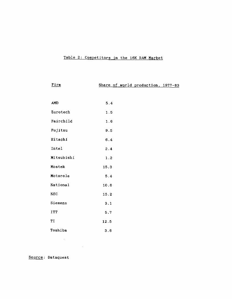
Table 2: Competitors in the 16K RAM Market

Firm Share of world production, 1977—83

A.MD 5.4

Eurotech 1.5

Fairchild 1.6

Fujitsu 9.5

Hitachi 6.4

Intel 2.4

Mitsubishi 1.2

Mostek 15.3

Motorola 5.4

National 10.6

NEC 15.2

Siemens 3.1

ITT 5.7

TI 12.5

Toshiba 3.6

Source: Dataquest

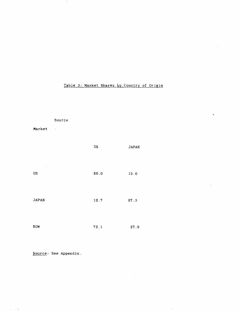
Table 3: Market Shares by Country of Origin

Source

Market

US JAPAN

US 88.0 12.0

JAPAN 12.7 87.3

ROW 72.1 27.9

Source: See Appendix.

Table 4: Market Shares and Sales Per Firm

A Market shares

Producer

Market

US JAPAN

US&ROW 14.0 5.3

JAPAN 2.1 29.1

B. Sales (million units)

Producer

Market

US JAPAN

US&ROW 23.95 9.13

JAPAN 1.5 20.4

Source: Table 3, Finan and Amundsen(1985), Dataquest.

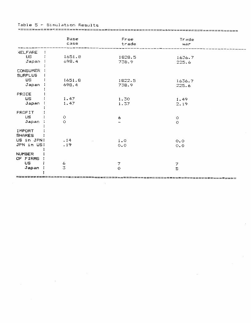
Table 5 — Simulation Results

Base Free Tradecase trade

4ELFAREUS 1b51.8 1828.5 1636.7Japan 698.4 738.9 225.6

CONSUMERSURPLUS

US 1651.8 1822,5 1634.7Japan 498.4 738,9 225.6

PRICEUS 1.47 1.3(1 1.49Japan 1.47 1.37 2.19

PROFITUS () 0Japan 0 C)

IMPORTSHARESUS i n J PN . 14 1 . 0 0. C)JF'N i n US . 1 9 0. 0 C) - 0

NUMBEROF FIRMS

US 6 7 7Japan 0 5