NBER WORKING PAPER SERIES

CAN CURRENCY COMPETITION WORK?

Jesús Fernández-VillaverdeDaniel Sanches

Working Paper 22157http://www.nber.org/papers/w22157

NATIONAL BUREAU OF ECONOMIC RESEARCH1050 Massachusetts Avenue

Cambridge, MA 02138April 2016

We thank Todd Keister and Guillermo Ordoñez for useful comments. The views expressed in this paper are those of the authors and do not necessarily reflect those of the Federal Reserve Bank of Philadelphia, the Federal Reserve System, or the National Bureau of Economic Research. Lastly, we also thank the NSF for financial support.

NBER working papers are circulated for discussion and comment purposes. They have not been peer-reviewed or been subject to the review by the NBER Board of Directors that accompanies official NBER publications.

© 2016 by Jesús Fernández-Villaverde and Daniel Sanches. All rights reserved. Short sections of text, not to exceed two paragraphs, may be quoted without explicit permission provided that full credit, including © notice, is given to the source.

Can Currency Competition Work?Jesús Fernández-Villaverde and Daniel SanchesNBER Working Paper No. 22157April 2016JEL No. E40,E42,E52

ABSTRACT

Can competition among privately issued fiat currencies such as Bitcoin or Ethereum work? Only sometimes. To show this, we build a model of competition among privately issued fiat currencies. We modify the current workhorse of monetary economics, the Lagos-Wright environment, by including entrepreneurs who can issue their own fiat currencies in order to maximize their utility. Otherwise, the model is standard. We show that there exists an equilibrium in which price stability is consistent with competing private monies, but also that there exists a continuum of equilibrium trajectories with the property that the value of private currencies monotonically converges to zero. These latter equilibria disappear, however, when we introduce productive capital. We also investigate the properties of hybrid monetary arrangements with private and government monies, of automata issuing money, and the role of network effects.

Jesús Fernández-VillaverdeUniversity of Pennsylvania160 McNeil Building3718 Locust WalkPhiladelphia, PA 19104and NBERjesusfv@econ.upenn.edu

Daniel SanchesFederal Reserve Bank of PhiladelphiaTen Independence MallPhiladelphia, PA 19106-1574Daniel.Sanches@phil.frb.org

1 Introduction

Can competition among privately issued fiat currencies work? The sudden appearance

of Bitcoin, Ethereum, and other cryptocurrencies has triggered a wave of public interest in

privately issued monies.1 A similar interest in the topic has not been seen, perhaps, since the

vivid polemics associated with the demise of free banking in the English-speaking world in

the middle of the 19th century (White, 1995). Somewhat surprisingly, this interest has not

translated, so far, into much research within monetary economics. Most papers analyzing the

cryptocurrency phenomenon have either been descriptive (Bohme, Christin, Edelman, and

Moore, 2015) or have dealt with governance and regulatory concerns from a legal perspective

(Chuen, 2015).2 In comparison, there has been much research related to the computer science

aspects of the phenomenon (Narayanan, Bonneau, Felten, Miller, and Goldfeder, 2016).

This situation is unfortunate. Without a theoretical understanding of how currency com-

petition works, we cannot answer a long list of positive and normative questions. Among the

positive questions: Will a system of private money deliver price stability? Will one currency

drive all others from the market? Or will several of these currencies coexist along the equi-

librium path? Will the market provide the socially optimum amount of money? Can private

monies and a government-issued money compete? Do private monies require a commodity

backing? Can a unit of account be separated from a medium of exchange? Among the

normative questions: Should governments prevent the circulation of private monies? Should

governments treat private monies as currencies or as any other regular property? Should the

private monies be taxed? Even more radically, now that cryptocurrencies are technically fea-

sible, should we revisit Friedman and Schwartz’s (1986) celebrated arguments justifying the

role of governments as money issuers? There are even questions relevant for entrepreneurs:

What is the best strategy to jump start the circulation of a currency? How do you maximize

the seigniorage that comes from it?

To address some of these questions, we build a model of competition among privately

issued fiat currencies. We modify the workhorse of monetary economics, the Lagos and

Wright (2005) (LW) environment, by including entrepreneurs who can issue their own fiat

currencies in order to maximize their utility. Otherwise, the model is standard. Following LW

has two important advantages. First, since the model is particularly amenable to analysis, we

can derive many insights about currency competition. Second, the use of the LW framework

1As of April 3, 2016, besides Bitcoin, three other cryptocurrencies (Etherum, Ripple, and Litecoin) havemarket capitalizations over $100 million and another eleven between $10 and $100 million. Updated numbersare reported by https://coinmarketcap.com/. Following convention, we will use Bitcoin, with a capital B,to refer to the whole payment environment, and bitcoin, with a lower case b, to denote the currency units ofthe payment system. See Antonopoulos (2015) for a technical introduction to Bitcoin.

2Some exceptions are Chiu and Wong (2014) and Hendrickson, Hogan, and Luther (2016).

2

makes our many new results easy to compare with previous findings in the literature.

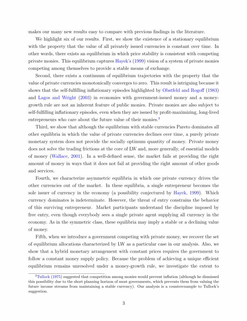
We highlight six of our results. First, we show the existence of a stationary equilibrium

with the property that the value of all privately issued currencies is constant over time. In

other words, there exists an equilibrium in which price stability is consistent with competing

private monies. This equilibrium captures Hayek’s (1999) vision of a system of private monies

competing among themselves to provide a stable means of exchange.

Second, there exists a continuum of equilibrium trajectories with the property that the

value of private currencies monotonically converges to zero. This result is intriguing because it

shows that the self-fulfilling inflationary episodes highlighted by Obstfeld and Rogoff (1983)

and Lagos and Wright (2003) in economies with government-issued money and a money-

growth rule are not an inherent feature of public monies. Private monies are also subject to

self-fulfilling inflationary episodes, even when they are issued by profit-maximizing, long-lived

entrepreneurs who care about the future value of their monies.3

Third, we show that although the equilibrium with stable currencies Pareto dominates all

other equilibria in which the value of private currencies declines over time, a purely private

monetary system does not provide the socially optimum quantity of money. Private money

does not solve the trading frictions at the core of LW and, more generally, of essential models

of money (Wallace, 2001). In a well-defined sense, the market fails at providing the right

amount of money in ways that it does not fail at providing the right amount of other goods

and services.

Fourth, we characterize asymmetric equilibria in which one private currency drives the

other currencies out of the market. In these equilibria, a single entrepreneur becomes the

sole issuer of currency in the economy (a possibility conjectured by Hayek, 1999). Which

currency dominates is indeterminate. However, the threat of entry constrains the behavior

of this surviving entrepreneur. Market participants understand the discipline imposed by

free entry, even though everybody sees a single private agent supplying all currency in the

economy. As in the symmetric class, these equilibria may imply a stable or a declining value

of money.

Fifth, when we introduce a government competing with private money, we recover the set

of equilibrium allocations characterized by LW as a particular case in our analysis. Also, we

show that a hybrid monetary arrangement with constant prices requires the government to

follow a constant money supply policy. Because the problem of achieving a unique efficient

equilibrium remains unresolved under a money-growth rule, we investigate the extent to

3Tullock (1975) suggested that competition among monies would prevent inflation (although he dismissedthis possibility due to the short planning horizon of most governments, which prevents them from valuing thefuture income streams from maintaining a stable currency). Our analysis is a counterexample to Tullock’ssuggestion.

3

which the presence of government money can simultaneously promote stability and efficiency

under an alternative policy rule. In particular, we study the properties of a policy rule that

pegs the real value of government money. Under this alternative regime, the properties of

the dynamic system substantially change as we vary the policy parameter determining the

target for the real value of government money. We show that it is possible to implement an

efficient allocation as the unique global equilibrium, but this requires driving private money

out of the economy.

Sixth, we study the situation where the entrepreneurs use productive capital. We can

think about this case as an entrepreneur, for example, issuing money to be used for purchases

of goods on her internet platform. The presence of productive capital fundamentally changes

the properties of the dynamic system describing the evolution of the real value of private

currencies. Autarky is no longer a steady state and, as a result, there can be no equilibrium

with the property that the value of private currencies converges to zero. Furthermore, it is

possible to obtain an allocation that is arbitrarily close to the efficient one as the unique

equilibrium provided capital is sufficiently productive. This allocation vindicates Hayek’s

proposal. It also links our research to the literature on the provision of liquidity by productive

firms (Holmstrom and Tirole, 2011, and Dang, Gorton, Holmstrom, and Ordonez, 2014).

We have further results involving automata issuing currency (inspired by the software

protocol behind Bitcoin and other cryptocurrencies) and the possible role of network effects

on currency circulation, but in the interest of space, we delay their discussion until later in

the paper.

The careful reader might have noticed that we have used the word “entrepreneur” and not

the more common “banker” to denote the issuers of private money. We believe this linguistic

turn is important. Our model highlights how the issuing of a private currency is logically

separated from banking. Both tasks were historically linked for logistical reasons: banks

had a central location in the network of payments that made it easy for them to introduce

currency in circulation. We will argue that the internet has broken the logistical barrier. The

issuing of bitcoins, for instance, is done through a proof-of-work system that is independent

of any banking activity (or at least of banking understood as the issuing and handling of

deposits and credit).4

This previous explanation may also address a second concern of this enlightened reader:

What are the differences between private monies issued in the past by banks (such as during

the Scottish free banking experience between 1716 and 1845) and modern cryptocurrencies?

As we mentioned, a first difference is the distribution process, which is now much wider and

4Similarly, some of the community currencies that have achieved a degree of success do not depend onbanks backing or issuing them (see Greco, 2001).

4

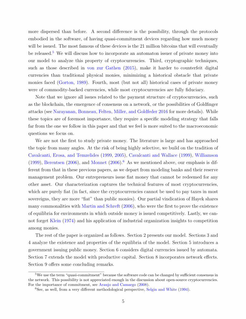
more dispersed than before. A second difference is the possibility, through the protocols

embodied in the software, of having quasi-commitment devices regarding how much money

will be issued. The most famous of these devices is the 21 million bitcoins that will eventually

be released.5 We will discuss how to incorporate an automaton issuer of private money into

our model to analyze this property of cryptocurrencies. Third, cryptographic techniques,

such as those described in von zur Gathen (2015), make it harder to counterfeit digital

currencies than traditional physical monies, minimizing a historical obstacle that private

monies faced (Gorton, 1989). Fourth, most (but not all) historical cases of private money

were of commodity-backed currencies, while most cryptocurrencies are fully fiduciary.

Note that we ignore all issues related to the payment structure of cryptocurrencies, such

as the blockchain, the emergence of consensus on a network, or the possibilities of Goldfinger

attacks (see Narayanan, Bonneau, Felten, Miller, and Goldfeder 2016 for more details). While

these topics are of foremost importance, they require a specific modeling strategy that falls

far from the one we follow in this paper and that we feel is more suited to the macroeconomic

questions we focus on.

We are not the first to study private money. The literature is large and has approached

the topic from many angles. At the risk of being highly selective, we build on the tradition of

Cavalcanti, Erosa, and Temzelides (1999, 2005), Cavalcanti and Wallace (1999), Williamson

(1999), Berentsen (2006), and Monnet (2006).6 As we mentioned above, our emphasis is dif-

ferent from that in these previous papers, as we depart from modeling banks and their reserve

management problem. Our entrepreneurs issue fiat money that cannot be redeemed for any

other asset. Our characterization captures the technical features of most cryptocurrencies,

which are purely fiat (in fact, since the cryptocurrencies cannot be used to pay taxes in most

sovereigns, they are more “fiat” than public monies). Our partial vindication of Hayek shares

many commonalities with Martin and Schreft (2006), who were the first to prove the existence

of equilibria for environments in which outside money is issued competitively. Lastly, we can-

not forget Klein (1974) and his application of industrial organization insights to competition

among monies.

The rest of the paper is organized as follows. Section 2 presents our model. Sections 3 and

4 analyze the existence and properties of the equilibria of the model. Section 5 introduces a

government issuing public money. Section 6 considers digital currencies issued by automata.

Section 7 extends the model with productive capital. Section 8 incorporates network effects.

Section 9 offers some concluding remarks.

5We use the term “quasi-commitment” because the software code can be changed by sufficient consensus inthe network. This possibility is not appreciated enough in the discussion about open-source cryptocurrencies.For the importance of commitment, see Araujo and Camargo (2008).

6See, as well, from a very different methodological perspective, Selgin and White (1994).

5

2 Model

The economy consists of a large number of buyers and sellers, with a [0, 1]-continuum

of each type, and a countable infinity of entrepreneurs. Each period is divided into two

subperiods. In the first subperiod, all types interact in a centralized market (CM) where a

perishable good, referred to as the CM good, is produced and consumed. Buyers and sellers

can produce the CM good by using a linear technology that requires effort as input. All

agents want to consume the CM good.

In the second subperiod, buyers and sellers interact in a decentralized market (DM)

characterized by pairwise meetings, with entrepreneurs remaining idle. In particular, a buyer

is randomly matched with a seller with probability σ ∈ (0, 1) and vice versa. In the DM,

buyers want to consume, but cannot produce, whereas sellers are able to produce, but do

not want to consume. A seller is able to produce a perishable good, referred to as the DM

good, using a divisible technology that delivers one unit of the good for each unit of effort he

exerts. An entrepreneur is neither a producer nor a consumer of the DM good.

Entrepreneurs are endowed with a technology to create tokens, which can take either a

physical or an electronic form. The essential feature of the tokens is that their authenticity

can be publicly verified at zero cost (for example, thanks to the application of cryptography

techniques), so that counterfeiting will not be an issue. As we will see, this technology will

permit entrepreneurs to issue tokens that can circulate as a medium of exchange.

Let us now explicitly describe preferences. Start with a typical buyer. Let xbt ∈ R denote

net consumption of the CM good, and let qt ∈ R+ denote consumption of the DM good. A

buyer’s preferences are represented by

U b(xbt , qt

)= xbt + u (qt) .

The utility function u : R+ → R is continuously differentiable, increasing, and strictly con-

cave, with u′ (0) = ∞ and u (0) = 0. Consider now a typical seller. Let xst ∈ R denote net

consumption of the CM good, and let nt ∈ R+ denote the seller’s effort level to produce the

DM good. A seller’s preferences are represented by

U s (xst , nt) = xst − w (nt) .

Assume that w : R+ → R+ is continuously differentiable, increasing, and weakly convex, with

w (0) = 0. Finally, let xit ∈ R+ denote entrepreneur i’s consumption of the CM good, with

6

i ∈ {1, 2, 3, ...}. Entrepreneur i has preferences represented by

∞∑t=0

βtxit.

The discount factor β ∈ (0, 1) is common across all types.

Throughout the analysis, we assume that buyers and sellers are anonymous (i.e., their

identities are unknown and their trading histories are privately observable), which precludes

credit in the decentralized market. In contrast, an entrepreneur’s trading history can be

publicly observable (i.e., an entrepreneur is endowed with a record-keeping technology that

permits him to reveal costlessly his trading history). As we will argue below, public knowledge

of an entrepreneur’s trading history will permit the circulation of private currencies.

3 Perfect Competition

Because the meetings in the DM are anonymous, there is no scope for trading future

promises in this market. As a result, a medium of exchange is essential to achieve allocations

that we could not achieve without it. In a typical monetary model, a medium of exchange is

supplied in the form of a government issued fiat currency, with the government following a

monetary policy rule (e.g., money-growth rule). Also, all agents in the economy can observe

the money supply at each date. These features allow agents to form beliefs about the exchange

value of money in the current and future periods.

We start our analysis by considering the possibility of a purely private monetary arrange-

ment. In particular, we focus on a system in which entrepreneurs issue intrinsically worthless

tokens that circulate as a medium of exchange, attaining a strictly positive value. These

privately issued currencies are not associated with any promise to exchange them for goods

at some future date. Because the currency issued by an entrepreneur is nonfalsifiable and an

entrepreneur’s trading history is publicly observable, all agents can verify the total amount

put into circulation by any individual issuer.

Profit maximization will determine the money supply in the economy. Since all agents

know that an entrepreneur enters the currency-issuing business to maximize profits, one

can describe individual behavior by solving the entrepreneur’s optimization problem in the

market for private currencies. These predictions about individual behavior allow agents to

form beliefs regarding the exchange value of private currencies, given the observability of

individual issuances. In other words, profit maximization in a private money arrangement

serves the same purpose as the monetary policy rule in the case of a government monopoly

7

on currency issue. As a result, it is possible to conceive a system in which privately issued

currencies can attain a positive exchange value.

In our analysis, a monetary unit comes in several brands issued by competing entrepreneurs.

Let φit ∈ R+ denote the value of a “dollar” issued by entrepreneur i ∈ {1, 2, 3, ...} in terms

of the CM good. Because there is free entry in the currency-issuing business and the op-

erational cost for an entrepreneur is zero, the number of entrepreneurs in the market will

be indeterminate. Throughout the paper, we restrict attention to equilibria in which a

fixed number N ∈ {1, 2, 3, ...} of entrepreneurs enter the market for private currencies, with

φt =(φ1t , ..., φ

Nt

)∈ RN

+ denoting the vector of real prices. We refer to those who enter the

currency-issuing business as active entrepreneurs.7

3.1 Buyer

Let us start by describing the portfolio problem of a typical buyer. Let W b (m, t) denote

the value function for a buyer holding a portfolio m =(m1, ...,mN

)∈ RN

+ of privately issued

currencies in the CM, and let V b (m, t) denote the value function in the DM. The Bellman

equation can be written as

W b (m, t) = max(x,m)∈R×RN+

[x+ V b (m, t)

]subject to the budget constraint

φt · m + x = φt ·m.

The vector m ∈ RN+ describes the buyer’s monetary portfolio after trading in the CM, and

x ∈ R denotes net consumption of the CM good. The value function W b (m, t) can be written

as

W b (m, t) = φt ·m +W b (0, t) ,

with the intercept given by

W b (0, t) = maxm∈RN+

[−φt · m + V b (m, t)

]. (1)

The value for a buyer holding a portfolio m in the DM is given by

V b (m, t) = σ[u (q (m, t)) + βW b (m− d (m, t) , t+ 1)

]+ (1− σ) βW b (m, t+ 1) , (2)

7It would be easy to extend the model to situations where the operational costs of running a currencyare positive, which will pin down the number of entrepreneurs in equilibrium.

8

with {q (m, t) ,d (m, t)} representing the terms of trade. Specifically, q (m, t) ∈ R+ denotes

production of the DM good and d (m, t) =(d1 (m, t) , ..., dN (m, t)

)∈ RN

+ denotes the vector

of currencies the buyer transfers to the seller. Because W b (m, t) = φt ·m +W b (0, t), we can

rewrite (2) as

V b (m, t) = σ[u (q (m, t))− β × φt+1 · d (m, t)

]+ β × φt+1 ·m + βW b (0, t+ 1) .

The standard approach in the search-theoretic literature determines the terms of trade

by Nash bargaining. Lagos and Wright (2005) demonstrate that Nash bargaining can result

in a holdup problem, leading to inefficient trading activity in the DM. Aruoba, Rocheteau,

and Waller (2007) consider alternative axiomatic bargaining solutions and conclude that the

properties of these solutions matter for the efficiency of monetary equilibrium. To avoid

inefficiencies arising from the choice of the bargaining protocol, which may complicate the

interpretation of the main results in the paper, we assume the buyer makes a take-it-or-leave-it

offer to the seller.8

With take-it-or-leave-it offers, the buyer chooses the amount of the DM good, represented

by q ∈ R+, the seller is supposed to produce and the vector of currencies, represented by

d =(d1, ..., dN

)∈ RN

+ , to be transferred to the seller to maximize expected surplus in the

DM. Formally, the terms of trade (q,d) are determined by solving

max(q,d)∈RN+1

+

[u (q)− β × φt+1 · d

]subject to the seller’s participation constraint

−w (q) + β × φt+1 · d ≥ 0

and the buyer’s liquidity constraint

d ≤m. (3)

Let q∗ ∈ R+ denote the quantity satisfying u′ (q∗) = w′ (q∗) (i.e., q∗ is the surplus-maximizing

quantity). The solution to the buyer’s problem is given by

q (m, t) =

{w−1

(β × φt+1 ·m

)if φt+1 ·m < β−1w (q∗) ,

q∗ if φt+1 ·m ≥ β−1w (q∗) ,

8Lagos and Wright (2005) show that, with take-it-or-leave-it offers by the buyer, it is possible to achievethe socially efficient allocation provided the government implements the Friedman rule.

9

φt+1 · d (m,t) =

{φt+1 ·m if φt+1 ·m < β−1w (q∗) ,

β−1w (q∗) if φt+1 ·m ≥ β−1w (q∗) .

Note that the solution to the bargaining problem allows us to characterize real expenditures

in the DM, given by φt+1 ·d (m,t), as a function of the buyer’s portfolio, with the composition

of the basket of currencies transferred to the seller remaining indeterminate.

The indeterminacy of the portfolio of currencies transferred to the seller in the DM is

reminiscent of Kareken and Wallace (1981). These authors have established that, in the ab-

sence of portfolio restrictions and barriers to trade, the exchange rate between two currencies

is indeterminate in a flexible-price economy. In our framework, a similar result holds with

respect to privately issued currencies, given the absence of transaction costs when dealing

with different currencies in the CM.

Given the previously derived solution to the bargaining problem, the value function

V (m, t) takes the form

V b (m, t) = σ[u(w−1

(β × φt+1 ·m

))− β × φt+1 ·m

]+ β × φt+1 ·m + βW b (0, t+ 1)

if φt+1 ·m < β−1w (q∗) and the form

V b (m, t) = σ [u (q∗)− w (q∗)] + β × φt+1 ·m + βW b (0, t+ 1)

if φt+1 ·m ≥ β−1w (q∗). Then, the first-order conditions for the optimal portfolio choice are

−φit + V bi (m, t) ≤ 0,

with equality if mi > 0. If φit+1/φit < β−1 for all i, then the optimal portfolio choice satisfies

σu′ (q (m, t))

w′ (q (m, t))+ 1− σ =

φitβφit+1

(4)

for each brand i, with q (m, t) = w−1(β × φt+1 ·m

). These conditions imply that, in an

equilibrium with multiple currencies, the expected return on money must be equalized across

all valued currencies (i.e., all currencies for which mi > 0). In the absence of portfolio

restrictions, an agent is willing to hold in portfolio two alternative currencies only if they yield

the same rate of return, given that these assets are equally useful in facilitating exchange in

the DM.

10

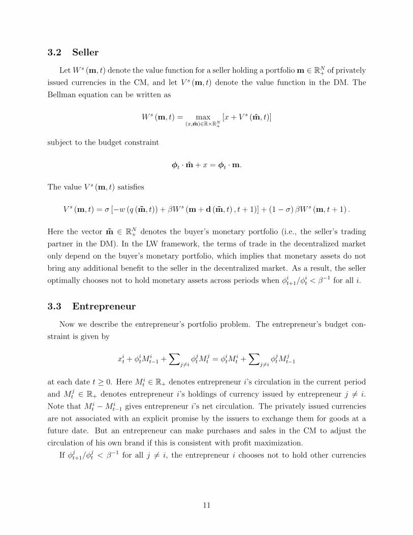
3.2 Seller

Let W s (m, t) denote the value function for a seller holding a portfolio m ∈ RN+ of privately

issued currencies in the CM, and let V s (m, t) denote the value function in the DM. The

Bellman equation can be written as

W s (m, t) = max(x,m)∈R×RN+

[x+ V s (m, t)]

subject to the budget constraint

φt · m + x = φt ·m.

The value V s (m, t) satisfies

V s (m, t) = σ [−w (q (m, t)) + βW s (m + d (m, t) , t+ 1)] + (1− σ) βW s (m, t+ 1) .

Here the vector m ∈ RN+ denotes the buyer’s monetary portfolio (i.e., the seller’s trading

partner in the DM). In the LW framework, the terms of trade in the decentralized market

only depend on the buyer’s monetary portfolio, which implies that monetary assets do not

bring any additional benefit to the seller in the decentralized market. As a result, the seller

optimally chooses not to hold monetary assets across periods when φit+1/φit < β−1 for all i.

3.3 Entrepreneur

Now we describe the entrepreneur’s portfolio problem. The entrepreneur’s budget con-

straint is given by

xit + φitMit−1 +

∑j 6=i

φjtMjt = φitM

it +

∑j 6=i

φjtMjt−1

at each date t ≥ 0. Here M it ∈ R+ denotes entrepreneur i’s circulation in the current period

and M jt ∈ R+ denotes entrepreneur i’s holdings of currency issued by entrepreneur j 6= i.

Note that M it −M i

t−1 gives entrepreneur i’s net circulation. The privately issued currencies

are not associated with an explicit promise by the issuers to exchange them for goods at a

future date. But an entrepreneur can make purchases and sales in the CM to adjust the

circulation of his own brand if this is consistent with profit maximization.

If φjt+1/φjt < β−1 for all j 6= i, the entrepreneur i chooses not to hold other currencies

11

across periods so that M jt = 0 for all j 6= i. Thus, we can rewrite the budget constraint as

xit + φitMit−1 = φitM

it

at each date t ≥ 0. In this case, the entrepreneur’s lifetime utility is given by

∞∑τ=t

βτ−tφiτ(M i

τ −M iτ−1

).

The entrepreneur’s lifetime utility derives from the currency-issuing business, given that

seigniorage is the only source of income (a privilege derived from access to the record-keeping

technologies). Consider a sequence of real prices{φit}∞t=0

with φit > 0 for all t ≥ 0. Then, we

must have

M it ≥M i

t−1

in every period t because consumption must be nonnegative. When φit > 0 for all t ≥ 0, it

follows that entrepreneur i’s money supply must be weakly increasing.

As previously mentioned, we assume free entry in the market for private currencies. In

the absence of operational costs, the free-entry condition implies

∞∑τ=t

βτ−tφiτ(M i

τ −M iτ−1

)= 0

at all dates t ≥ 0. This condition, together with nonnegative consumption xit ≥ 0 at all dates,

implies

φit(M i

t −M it−1

)= 0

at all dates t ≥ 0. If φit > 0 holds at all dates t ≥ 0, then the only feasible choice for

entrepreneur i is M it = M i

t−1 in every period. In other words, entrepreneur i must choose

M it = M i at all dates t ≥ 0, given some initial state M i

−1 = M i > 0. Along an equilibrium

trajectory, the nominal supply of each brand remains constant over time to make it consistent

with free entry. The market discipline imposed by free entry takes the form of a constant

nominal supply in the absence of operational costs. However, as we will see, the real value of

a unit of money issued by entrepreneur i can vary over time.

3.4 Equilibrium

We say that currency i is valued in equilibrium if φit > 0 for all t ≥ 0. If currency i is

valued, then we denote its real return by γit+1 ≡ φit+1/φit. In an equilibrium with the property

12

that currencies i and j coexist as a medium of exchange, condition (4) implies γit+1 = γjt+1

at all dates. Let γt+1 denote the common rate of return in an equilibrium with multiple

currencies (i.e., the common return across all currencies that are valued in equilibrium). If

γt+1 < β−1, then the liquidity constraint (3) is binding. Let qt ∈ R+ denote the quantity

traded in the DM in period t. We can rewrite the first-order conditions (4) as a single

condition

σu′ (qt)

w′ (qt)+ 1− σ =

1

βγt+1

. (5)

This condition determines production in a bilateral meeting as a function of the expected

return on money. Thus, we can use (5) to implicitly define qt = q(γt+1

), with q′ (γ) > 0 for

all γ > 0. Thus, a higher return on money results in a larger amount produced in the DM.

The demand for real balances is given by

z(γt+1

)≡w(q(γt+1

))βγt+1

. (6)

As we will see, the demand for real balances can be either increasing or decreasing in the rate

of return γt+1, depending on the specification of preferences and technologies.

In equilibrium, the market-clearing condition

N∑i=1

φitMit = z

(γt+1

)(7)

must hold in all periods t ≥ 0. The only asset market in the economy is the market for

privately issued currencies. A buyer rebalances his portfolio in the centralized market and a

seller exits the centralized market holding no assets. Because quasi-linear preferences imply

that all buyers have the same demand function, condition (6) provides the aggregate demand

for real balances. The real value of the money supply is obtained by summing up the real

value of each private currency.

Let bit ≡ φitMit denote the real value of the total supply of currency i in period t and let

bt ∈ RN+ denote the vector of real values in period t. Free entry in the market for private

currencies requires

bit − γtbit−1 = 0 (8)

for each i at all dates t ≥ 0. Finally, the market-clearing condition can be written as

N∑i=1

bit = z(γt+1

)(9)

13

at all dates t ≥ 0. Given these conditions, we can formally define an equilibrium in terms of

the sequence {bt, γt}∞t=0.

Definition 1 A perfect-foresight equilibrium is a sequence {bt, γt}∞t=0 satisfying (8), (9),

bit ≥ 0, and 0 ≤ γt ≤ β−1 for all t ≥ 0 and i ∈ {1, ..., N}.

It is a property of any equilibrium allocation that the exchange rate among private curren-

cies remains indeterminate: the solution to the bargaining problem allows us to derive total

real expenditures in the DM, but not the composition of the monetary portfolio transferred

to the seller. As previously mentioned, this result is a direct consequence of the absence of

portfolio restrictions and transaction costs.

4 Existence

We start our analysis by characterizing symmetric equilibria with the property bit = bjt for

all i and j. In these equilibria, all active entrepreneurs issue currencies that circulate as a

medium of exchange, with the market for privately issued currencies equally divided among

them. The following proposition formally establishes the existence of symmetric equilibria.

Proposition 1 There exists a continuum of equilibrium trajectories with the property bit = bjt

for all i and j at all dates t ≥ 0. These equilibria can be characterized by a sequence {γt}∞t=0

satisfying

z(γt+1

)= γtz (γt) (10)

and 0 ≤ γt ≤ β−1 at all dates t ≥ 0.

Proof. Because bit = bjt for all i and j, the market-clearing condition reduces to

Nbt = z(γt+1

)for some common value bt ≥ 0. Free entry implies bt = γtbt−1 at each date t ≥ 0. Thus,

a symmetric equilibrium can be defined as a sequence {γt}∞t=0 satisfying (10). This equa-

tion implicitly defines a mapping γt+1 = f (γt) with at least two fixed points: the origin(γt, γt+1

)= (0, 0) and the interior steady state

(γt, γt+1

)= (1, 1). As a result, there exists

a continuum of equilibrium trajectories that can be constructed starting from any arbitrary

point γ0 ∈ (0, 1).

An immediate consequence of the previous proposition is the existence of a stationary

equilibrium with the property that the value of all privately issued currencies is constant over

14

time. Or more plainly: there exists an equilibrium in which price stability is consistent with

competing private monies.

Corollary 2 There exists an interior stationary equilibrium with γt = 1 for all t ≥ 0.

Proof. As we have seen, equation (10) implicitly defines a mapping γt+1 = f (γt) for

which(γt, γt+1

)= (1, 1) is a fixed point. Thus, setting γt = 1 for all t ≥ 0 is a solution

satisfying the boundary condition 0 ≤ γt ≤ β−1.

In this equilibrium, the exchange value of private currencies remains stable over time.

Agents do not expect monetary conditions to vary over time so that the real value of private

currencies, as well as their expected return, remains constant. Thus, it is possible to have

an equilibrium with stable currencies, even though these privately issued tokens are not

associated with any explicit promise to exchange them for goods at some future date. Our

analysis finds that the type of purely private arrangement initially envisaged by Hayek (1999)

is feasible. Hayek argued that private agents through markets can achieve desirable outcomes,

even in the field of money and banking. According to his view, government intervention is

not necessary for the establishment of a stable monetary system.

However, we will show momentarily that other allocations with undesirable properties can

also be consistent with the same equilibrium conditions. These equilibria are characterized by

the persistently declining purchasing power of private currencies and falling trading activity.

There is no reason to forecast that the equilibrium with stable value will prevail over these

different equilibria.

Furthermore, even the equilibrium with a stable value of currencies is socially inefficient.

In this equilibrium, the quantity traded in the DM q satisfies

σu′ (q)

w′ (q)+ 1− σ =

1

β,

which is below the socially efficient quantity (i.e., q < q∗). Although the equilibrium with

stable currencies Pareto dominates all other equilibria in which the value of private currencies

declines over time, a purely private monetary system does not provide the socially optimum

quantity of money, as defined in Friedman (1969).

Our next step is to characterize nonstationary equilibria with the property that the value of

privately issued currencies collapses along the equilibrium path. At this point, it makes sense

to restrict attention to preferences and technologies that imply an empirically plausible money

demand function satisfying the property that the demand for real balances is decreasing in

the inflation rate (i.e., increasing in the real return on money). In particular, it is helpful to

15

assume that u (q) = (1− η)−1 q1−η and w (q) = (1 + α)−1 q1+α, with 0 < η < 1 and α ≥ 0. In

this case, the demand for real balances satisfies

z(γt+1

)=

(βγt+1

) 1+αη+α−1

1 + α

[σ

1− (1− σ) βγt+1

] 1+αη+α

.

Note that z′ (γ) > 0 for all γ > 0 so that the demand for real balances is increasing in the real

return on money. The dynamic system describing the equilibrium evolution of γt is given by

γ1+αη+α−1

t+1[1− (1− σ) βγt+1

] 1+αη+α

=γ

1+αη+α

t

[1− (1− σ) βγt]1+αη+α

. (11)

Because the initial choice γ0 is arbitrary, there exist multiple equilibrium trajectories that

converge monotonically to autarky.9

Proposition 2 Suppose u (q) = (1− η)−1 q1−η and w (q) = (1 + α)−1 q1+α, with 0 < η < 1

and α ≥ 0. Then, there exists a continuum of equilibrium trajectories starting from any

γ0 ∈ (0, 1) with the property that the value of private money monotonically converges to zero.

Proof. Note that γt = 0 when γt+1 = 0 because the demand function z (γ) goes to zero

as γ converges to zero from above. When γt+1 = β−1, it follows that γt < β−1. Using the

Implicit Function Theorem, we have

dγtdγt+1

=z′(γt+1

)γtz′ (γt) + z (γt)

> 0

for any γt+1 ∈[0, β−1

]. The Inverse Function Theorem implies

dγt+1

dγt=γtz′ (γt) + z (γt)

z′(γt+1

) > 0

for any γt ∈[0, f−1

(β−1)]

, so the implicitly defined mapping γt+1 = f (γt) is strictly increas-

ing. In particular, we have

dγt+1

dγt

∣∣∣∣γt=γt+1=1

=z′ (1) + z (1)

z′ (1)> 1,

which means that the mapping γt+1 = f (γt) crosses the 45-degree line from below at the

point(γt, γt+1

)= (1, 1). Thus, the unique interior stationary solution is given by γt = 1 for

9Sanches (2016) has derived a similar result in an economy with the property that entrepreneurs issuedebt claims that circulate as a medium of exchange.

16

all t ≥ 0. In this case, a seller is willing to produce the quantity q satisfying

σu′ (q)

w′ (q)+ 1− σ = β−1.

For any initial choice γ0 ∈ (0, 1), the mapping γt+1 = f (γt) yields a strictly decreasing

sequence {γt}∞t=0 with the property limt→∞ γt = 0.

Figure 1 plots the dynamic system (11) with α = .5, β = .9, η = .5, and σ = .9. For

any initial condition γ0 ∈ (0, 1), there exists an associated equilibrium trajectory that is

monotonically decreasing. Along this equilibrium path, real money balances decrease mono-

tonically over time and converge to zero, so the equilibrium allocation approaches autarky

as t→∞. The decline in the desired amount of real balances follows from the agent’s opti-

mization problem when the value of privately issued currencies persistently depreciates over

time (i.e., the anticipated decline in the purchasing power of private money leads agents to

reduce their real money balances over time). As a result, trading activity in the decentralized

market monotonically declines along the equilibrium trajectory. This property of equilibrium

allocations with privately issued currencies implies that private money is inherently unstable

in that changes in beliefs can lead to undesirable self-fulfilling inflationary episodes.

Figure 1: Dynamic system (11)

17

The existence of these inflationary equilibrium trajectories in a purely private mone-

tary arrangement implies that hyperinflationary episodes are not an exclusive property of

government-issued money. Obstfeld and Rogoff (1983) build economies that can display self-

fulfilling inflationary episodes when the government is the sole issuer of currency and follows

a money-growth rule. Lagos and Wright (2003) show that search-theoretic monetary models

with government-supplied currency can also have self-fulfilling inflationary episodes under a

money-growth rule. Our analysis of privately issued currencies shows that self-fulfilling infla-

tionary equilibria can occur in the absence of government currency when private agents enter

the currency-issuing business to maximize profits. Thus, replacing government monopoly

under a money-growth rule with free entry and profit maximization does not overcome the

fundamental fragility associated with fiduciary regimes, public or private.

In the following section, we introduce government currency and study the possibility of

stabilization policies. As we will see, the set of equilibrium allocations characterized by LW

arises as a special case in our analysis. In addition, we will study the equilibrium interaction

between private and government monies and derive some interesting properties.

As previously mentioned, the stationary equilibrium with a stable value of private cur-

rencies Pareto dominates any nonstationary equilibria, even though that equilibrium does

not achieve the first best. To verify this claim, note that the quantity traded in the DM

starts from a value below q and decreases monotonically in a nonstationary equilibrium. As

a result, the allocation in the equilibrium with a stable value of money Pareto dominates the

allocation associated with any inflationary equilibrium.

Now we turn to asymmetric equilibria. Given that utility is linear and transferable in

the CM, the allocation in the DM is what matters for the welfare analysis. However, we

are still interested in studying the CM allocation in our positive analysis of currency com-

petition. Given that the production of tokens costs nothing, there is no condition to pin

down the market share of each active entrepreneur, represented by the real values bit, in the

market for private currencies. Although the indeterminacy of the market share has no welfare

consequences, we want to study some asymmetric equilibria in our positive analysis.

An asymmetric equilibrium of interest involves a unique private currency circulating in the

economy, despite free entry. The following proposition shows that any equilibrium allocation

can be characterized by the dynamic system (10) and that it is possible to construct an

equilibrium in which a unique private currency dominates other currencies as a medium of

exchange, even though there is free entry in the currency-issuing business. Again, this occurs

because the market shares across different types of money are indeterminate.

Proposition 3 An equilibrium allocation can be characterized by a sequence {γt}∞t=0 satis-

fying (10) and the boundary condition 0 ≤ γt ≤ β−1 at all dates. In particular, there exists

18

an equilibrium with valued money satisfying b1t = bt > 0 and bit = 0 for all i ≥ 2 at all dates

t ≥ 0.

Proof. Because (8) must hold for all i, we have

N∑i=1

bit = γt

N∑i=1

bit−1.

Condition (9) impliesN∑i=1

bit = z(γt+1

).

Thus, the dynamic system (10), together with the boundary condition 0 ≤ γt ≤ β−1, describes

the evolution of the real return on money γt in any equilibrium. As we have seen, condition

(5) implies that the sequence {γt}∞t=0 determines the equilibrium allocation in the DM.

Note that bjt = 0 implies either φjt = 0 or M jt = 0, or both. Because bit = 0 for all i ≥ 2,

the market-clearing condition implies b1t = z

(γt+1

). Free entry requires that the sequence

of returns {γt}∞t=0 satisfy (10). Hence, there exists an equilibrium with b1

t = z (1) > 0 and

bit = 0 for all i ≥ 2 at all dates t ≥ 0. In addition, there exists a continuum of equilibria with

b1t = z

(γt+1

)> 0 and bit = 0 for all i ≥ 2 at all dates t ≥ 0, with {γt}

∞t=0 representing any

sequence that solves (10) starting from an arbitrary point γ0 ∈ (0, 1).

In these equilibria, a single entrepreneur becomes the sole issuer of currency in the econ-

omy. The threat of entry constrains his behavior and market participants understand the

discipline imposed by free entry, even though all agents see a single private agent supplying

all currency in the economy. As in the symmetric class, an equilibrium with a stable value

of money is as likely to occur as an equilibrium with a declining value of money.

5 Government

In this section, we study the interaction between private and government monies and the

possibility of monetary stabilization through public policy. Suppose the government enters

the currency-issuing business by creating its own brand. The government budget constraint

is given by

φtMt + τ t = φtMt−1,

where τ t ∈ R is the real value of lump-sum taxes, φt ∈ R+ is the real value of government-

issued currency, and Mt ∈ R+ is the amount supplied at date t. What makes government

19

money fundamentally different from private money is that behind the government brand there

is a fiscal authority with the power to tax agents in the economy.

5.1 Money-growth rule

We start by assuming that the government follows a money-growth rule of the form

Mt = (1 + ω) Mt−1,

with ω ≥ β − 1. In any equilibrium with valued government money, we must have

φt+1

φt= γt+1 (12)

at all dates t ≥ 0. Here γt+1 continues to represent the common rate of return across all

currencies that are valued in equilibrium. In the absence of portfolio restrictions, government

money must yield the same rate of return as other monetary assets for it to be valued in

equilibrium.

Let mt ≡ φtMt denote the real value of government-issued currency. Then, condition (12)

implies

mt = (1 + ω)mt−1γt (13)

at all dates. The market-clearing condition in the asset market becomes

mt +N∑i=1

bit = z(γt+1

)(14)

for all t ≥ 0. Given these changes in the equilibrium conditions, it is now possible to provide

a formal definition of equilibrium in the presence of government intervention.

Definition 3 Given the policy parameter ω, a perfect-foresight equilibrium is a sequence

{bt,mt, γt}∞t=0 satisfying (8), (13), (14), bit ≥ 0, mt ≥ 0, and 0 ≤ γt ≤ β−1 for all t ≥ 0 and

i ∈ {1, ..., N}.

We start our analysis of a hybrid monetary arrangement by characterizing equilibria

with the property bit = bjt = mt for all i and j. In these symmetric equilibria, private

and government monies attain the same exchange value. Our next result shows that an

equilibrium with this property exists if and only if the government follows the policy ω = 0

(i.e., constant government supply).

20

Proposition 4 A symmetric equilibrium with the property that private and government monies

attain the same value exists if and only if ω = 0. In this case, there exist multiple equilibrium

trajectories characterized by a sequence {γt}∞t=0 satisfying (10) and 0 ≤ γt ≤ β−1 at all dates

t ≥ 0.

Proof. Symmetry requires bit = mt for all i at all dates. Let bt denote the common value.

Thus, the market-clearing condition implies

bt =z(γt+1

)N + 1

.

Since the free-entry condition, bt−γtbt−1 = 0, must hold at all dates, the equilibrium evolution

of the real return on money γt must satisfy (10).

As previously mentioned, condition (12) implies mt = (1 + ω)mt−1γt. Because mt = bt

must hold in a symmetric equilibrium, we have

z(γt+1

)= (1 + ω) z (γt) γt.

This means that an equilibrium with the property that private and government monies attain

the same value exists if and only if ω = 0. As a result, an equilibrium sequence {γt}∞t=0 must

satisfy (10) and the boundary condition 0 ≤ γt ≤ β−1 at all dates.

The previous result implies that price stability with both private and government monies

circulating as competing media of exchange can be attained under a money-growth rule only

if the government maintains a constant supply of its own brand. As in the purely private

monetary economy, there exist multiple equilibrium trajectories with the property that the

value of money monotonically declines over time, converging to zero. Thus, the introduction of

the government brand under a money-growth rule does not resolve the instability of fiduciary-

currency regimes.

A natural question to ask is whether it is possible to have an equilibrium with both private

and government monies circulating in the economy when government policy deviates from

ω = 0. If ω 6= 0, then we have to consider the possibility of asymmetric equilibria with the

property that government money and private money have different values, even though both

monies yield the same rate of return. These equilibria can be characterized by a sequence

{bt,mt}∞t=0 satisfying

Nbt +mt = z(γt+1

), (15)

bt = γtbt−1, (16)

mt = (1 + ω)mt−1γt, (17)

21

together with the boundary conditions bt ≥ 0, mt ≥ 0, and 0 ≤ γt ≤ β−1. The following

proposition establishes that a hybrid monetary arrangement with a constant return on money

does not exist when the government pursues either an expansionary or a contractionary policy.

Proposition 5 There is no equilibrium with the properties that the return on monetary assets

remains constant over time and private and government monies coexist as media of exchange

when ω 6= 0.

Proof. Suppose that γt = γ for all t ≥ 0. Then, (16) implies, at all dates,

btbt−1

= γ.

Condition (17) implies, at all dates,

mt

mt−1

= (1 + ω) γ.

Finally, condition (15) requires, at all dates,

Nbt +mt = Nbt−1 +mt−1.

These conditions can be simultaneously satisfied if and only if ω = 0 and γ = 1.

The previous result implies that expansionary and contractionary policies are not con-

sistent with the coexistence of stable private and government monies (i.e., monetary assets

with the property that their returns remain constant over time). Thus, these assets cannot

jointly serve as stable media of exchange when the government deviates from the constant

money supply rule. Under a money-growth regime, the existence of a stable hybrid monetary

arrangement requires the government to follow a constant money supply rule.

As should be expected, it is possible to have equilibria with valued government money

only. In particular, we can construct asymmetric equilibria with the property bit = 0 for all i

and mt ≥ 0 at all dates t ≥ 0 (i.e., only government-issued currency circulates as a medium

of exchange). In these equilibria, the sequence of returns satisfies, for all dates

z(γt+1

)= (1 + ω) z (γt) γt. (18)

The dynamic properties of the system (18) are exactly the same as those derived in Lagos and

Wright (2003) when preferences and technologies imply a demand function for real balances

that is strictly decreasing in the inflation rate. For instance, selecting the functional forms

22

u (q) = (1− η)−1 q1−η and w (q) = (1 + α)−1 q1+α results in a dynamic system of the form

γ1+αη+α−1

t+1[1− (1− σ) βγt+1

] 1+αη+α

= (1 + ω)γ

1+αη+α

t

[1− (1− σ) βγt]1+αη+α

(19)

with 0 < η < 1 and α ≥ 0.

A policy choice ω in the range (β − 1, 0) is associated with a steady state characterized

by deflation and a strictly positive real return on money. In particular, γt = (1 + ω)−1 for all

t ≥ 0. In this stationary equilibrium, the quantity traded in the DM, represented by q (ω),

satisfies

σu′ (q (ω))

w′ (q (ω))+ 1− σ =

1 + ω

β.

Figure 2 plots the dynamic system (19) for several values of the money growth rate ω with

α = .5, β = .9, η = .5, and σ = .9.

Figure 2: Dynamic system (19)

If we let ω → β − 1, the associated steady state delivers an efficient allocation (i.e.,

q (ω) → q∗ as ω → β − 1). This policy prescription is the celebrated Friedman rule, which

eliminates the opportunity cost of holding money balances in private portfolios for transaction

purposes. The problem with this arrangement is that the Friedman rule is not uniquely

associated with an efficient allocation. There exists a continuum of suboptimal equilibrium

23

trajectories that are also associated with the Friedman rule. These trajectories involve a

persistently declining value of money.

5.2 Pegging the real value of government liabilities

In this section, we develop an alternative monetary policy rule that can implement a

unique efficient equilibrium allocation. This outcome will be feasible only if the government

can tax private agents to finance policy implementation. Also, it will require government

money to drive private money out of the economy.

Suppose the government decides to peg the real value of its monetary liabilities. Specifi-

cally, assume the government issues currency to satisfy

φtMt = m (20)

at all dates for some target value m > 0. This means that the government adjusts the money

supply sequence{Mt

}∞t=0

to satisfy (20) in each period. In this case, the market-clearing

condition in the asset market becomes

m+N∑i=1

bit = z(γt+1

)(21)

at all dates t ≥ 0.

Furthermore, we need to impose the boundary conditions bit ≥ 0 at all dates t ≥ 0 for

each i. These conditions imply

z (γt) ≥ m (22)

at all dates t ≥ 0. In other words, the policy of pegging the real value of government

money results in a lower bound for the real return on money in equilibrium. Given these

changes in the equilibrium conditions, we can now provide a definition of equilibrium when

the government pegs the real value of its monetary liabilities.

Definition 4 Given the policy parameter m > 0, a perfect-foresight equilibrium is a sequence

{bt, γt}∞t=0 satisfying (8), (21), (22), bit ≥ 0, and 0 ≤ γt ≤ β−1 for all t ≥ 0 and i ∈ {1, ..., N}.

Although the government supply is an endogenous variable, we do not need to include it

in our definition of equilibrium as it adjusts to satisfy (20) at each date. In particular, the

money supply sequence{Mt

}∞t=0

must satisfy

Mt+1 =1

γt+1

Mt

24

at all dates t ≥ 0. Because the monetary authority pegs the real value of its monetary liabil-

ities, the government money supply Mt varies over time to follow the equilibrium evolution

of the return on monetary assets, given the target value m.

The following proposition provides a useful characterization of equilibrium when the gov-

ernment pegs the real value of its liabilities. It also shows that the equilibrium with constant

prices is a steady state regardless of the choice of the policy parameter m.

Proposition 6 An equilibrium allocation can be characterized by a sequence {γt}∞t=0 satisfy-

ing

z(γt+1

)= γtz (γt)− γtm+m (23)

and the boundary conditions 0 ≤ γt ≤ β−1 and z (γt) ≥ m at all dates. In particular, the

stationary solution γt = 1 for all t ≥ 0 is an equilibrium trajectory for any value of the policy

parameter m.

Proof. Because (8) must hold for all i, we have

N∑i=1

bit = γt

N∑i=1

bit−1.

Condition (21) impliesN∑i=1

bit = z(γt+1

)−m.

Thus, the dynamic system (23), together with the boundary conditions 0 ≤ γt ≤ β−1 and

z (γt) ≥ m, describes the evolution of the return on money γt along the equilibrium path.

Finally, it is straightforward to show that(γt, γt+1

)= (1, 1) is a fixed point of the implicitly

defined mapping γt+1 = f (γt).

Note that autarky is no longer a steady state when m > 0, so the policy of pegging the real

value of government liabilities fundamentally changes the properties of the dynamic system.

To demonstrate the main result of this section, it is helpful to assume the functional forms

u (q) = (1− η)−1 q1−η and w (q) = (1 + α)−1 q1+α, with 0 < η < 1 and α ≥ 0. In this case,

the dynamic system (23) reduces to

σ1+αη+α(βγt+1

) 1+αη+α−1[

1− (1− σ) βγt+1

] 1+αη+α

=β

1+αη+α−1 (σγt)

1+αη+α

[1− (1− σ) βγt]1+αη+α

−mγt +m (24)

with(βγt)

1+αη+α−1

1 + α

[σ

1− (1− σ) βγt

] 1+αη+α

≥ m (25)

25

at all dates t ≥ 0. Condition (25) imposes a lower bound on the equilibrium return on money,

which can result in the existence of a steady state at the lower bound.

The properties of equations (24)-(25) depend on the value of the policy parameter m.

In particular the dynamic system (24)-(25) is a transcritical bifurcation.10 To illustrate this

property, it is helpful to simplify the dynamic system by assuming that α = 0 (linear disutility

of production) and σ → 1 (no matching friction in the decentralized market). In this case,

the equilibrium evolution of the return on money γt satisfies the law of motion

γt+1 = γ2t −

m

βγt +

m

β(26)

and the boundary conditionm

β≤ γt ≤

1

β. (27)

The policy parameter can take on any value in the interval 0 ≤ m ≤ 1. Also, the value of

money remains above the lower bound m at all dates. Given that the government provides a

credible lower bound for the value of money due to its taxation power, the return on money

is bounded below by a strictly positive constant β−1m along the equilibrium path.

We can obtain a steady state by solving the polynomial equation

γ2 −(m

β+ 1

)γ +

m

β= 0.

If m 6= β, the roots are 1 and β−1m. If m = β, the unique solution is 1. As we will see, the

properties of the dynamic system differ considerably depending on the value of the policy

parameter m.

If 0 < m < β, then there exist two steady states: γt = β−1m and γt = 1 for all t ≥ 0.

The steady state γt = 1 for all t ≥ 0 corresponds to the previously described stationary

equilibrium with constant prices. The steady state γt = β−1m for all t ≥ 0 is an equilibrium

with the property that only government money is valued. To see why this occurs, note that

z (γt) = z(β−1m

)= m holds in every period t so that we must have bit = 0 for each i

at all dates t ≥ 0. Figure 3 shows the dynamic system when 0 < m < β (panel (a) for

0 < γt < (1/β) and panel (b) for (m/β) < γt < (1/β)). In this case, the steady state with

a low value of money (β−1m) is globally stable. As we can see, there exists a continuum of

equilibrium trajectories starting from any point γ0 ∈(β−1m, 1

)with the property that the

10In bifurcation theory, a transcritical bifurcation is one in which a fixed point exists for all values of aparameter and is never destroyed. Both before and after the bifurcation, there is one unstable and one stablefixed point. However, their stability is exchanged when they collide, so the unstable fixed point becomesstable and vice versa.

26

return on money converges to β−1m. Along these trajectories, the value of money declines

monotonically to the lower bound m and government money drives private money out of the

economy.

(a) 0 < γt < (1/β) (b) (m/β) < γt < (1/β)

Figure 3: Dynamic system for government money, 0 < m < β

If m = β, the unique steady state is γt = 1 for all t ≥ 0. This case is represented in Figure

4 (again with panel (a) for 0 < γt < (1/β) and panel (b) for (m/β) < γt < (1/β)). Note that

the 45-degree line is the tangent line to the graph of (26) at the point (1, 1), so the dynamic

system remains above the 45-degree line. When we introduce the boundary restriction (27),

we find that γt = 1 for all t ≥ 0 is the unique equilibrium trajectory. Thus, the policy choice

m = β results in global determinacy, with the unique equilibrium outcome characterized by

price stability.

If β < m < 1 (Figure 5), the unique steady state is γt = β−1m for all t ≥ 0. When we

introduce the boundary restriction (27), γt = β−1m for all t ≥ 0 is the unique equilibrium

trajectory. Setting the target for the value of government money in the interval β < m < 1

results in a sustained deflation to ensure that the return on money remains above one. To

implement a sustained deflation, the government must contract its money supply, a policy

financed through taxation. Since a sustained contraction of the money supply by a private

entrepreneur is infeasible, in this situation there is only government money circulating in the

economy.

27

(a) 0 < γt < (1/β) (b) (m/β) < γt < (1/β)

Figure 4: Dynamic system for government money, m = β

To implement a target value in the range β < m < 1, the government must tax private

agents in the CM. To verify this claim, note that the government budget constraint can be

written as

τ t = m (γt − 1)

in every period t. Because the unique steady state implies γt = β−1m for all t ≥ 0, we must

have

τ t = m(β−1m− 1

)> 0

at all dates t ≥ 0. To implement its target value m, the government needs to persistently

shrink the money supply by making purchases that exceed its sales in the CM, with the

shortfall financed by taxes.

Finally, it is possible to implement an efficient allocation as the unique equilibrium out-

come when we take the limit m→ 1. Thus, the joint goal of monetary stability and efficiency

can be achieved by government policy. The only caveat is that the implementation of an

efficient allocation requires government money to drive private money out of the economy.

In a few pages we will see how government money will no longer be essential when private

entrepreneurs have access to sufficiently productive capital.

28

(a) 0 < γt < (1/β) (b) (m/β) < γt < (1/β)

Figure 5: Dynamic system for government money, β < m < 1

6 Automata

In this section, we introduce private currencies issued by automata. This extension of

the baseline model is motivated by the observation that digital currencies such as Bitcoin

are associated with software protocols that fix, in an automatic fashion, the total amount of

units of money that can be put into circulation.

Consider the benchmark economy described in Section 3 and add J automata, each pro-

grammed to issue a constant amount Hj ∈ R+ of tokens. Let hjt ≡ φjtHj denote the real

value of the tokens issued by automaton j ∈ {1, ..., J} and let ht ≡(h1t , ..., h

Jt

)∈ RJ

+ denote

the vector of real values. If the units issued by automaton j are valued in equilibrium, then

we must haveφjt+1

φjt= γt+1 (28)

at all dates t ≥ 0. Here γt+1 continues to represent the common real return across all

currencies that are valued in equilibrium. Thus, condition (28) implies

hjt = hjt−1γt (29)

29

for each j at all dates. The market-clearing condition in the asset market becomes

J∑i=1

hjt +N∑i=1

bit = z(γt+1

)(30)

for all t ≥ 0. Given these conditions, we can now provide a definition of equilibrium in the

presence of automata.

Definition 5 A perfect-foresight equilibrium is a sequence {bt,ht, γt}∞t=0 satisfying (8), (29),

(30), bit ≥ 0, hjt ≥ 0, and 0 ≤ γt ≤ β−1 for all t ≥ 0, i ∈ {1, ..., N}, and j ∈ {1, ..., J}.

Our main result in this section is to show that the set of equilibrium allocations in the

presence of automata is the same as in the economy with profit-maximizing entrepreneurs

only.

Proposition 7 The set of equilibrium allocations is the same as in the economy without

automata. In particular, an equilibrium trajectory is characterized by a sequence {γt}∞t=0

satisfying (10) and 0 ≤ γt ≤ β−1 at all dates t ≥ 0.

Proof. The free-entry condition implies bit = γtbit−1 for each i ∈ {1, ..., N} at all dates.

Then, we can derive the relation

N∑i=1

bit = γt

N∑i=1

bit−1.

From (29), we findJ∑i=1

hjt = γt

J∑i=1

hjt−1.

Then, the market-clearing condition implies

z(γt+1

)=

J∑i=1

hjt +N∑i=1

bit = γt

(N∑i=1

bit−1 +J∑i=1

hjt−1

)= γtz (γt)

as initially claimed. Because the sequence of returns {γt}∞t=0 determines the equilibrium

allocation, we obtain the equivalence result as claimed.

The result that the introduction of automata does not change the fundamental proper-

ties of the private monetary arrangement is not surprising given that a profit-maximizing

entrepreneur optimally chooses a constant nominal supply of his own brand in a perfectly

30

competitive environment. The commitment implied by a machine programmed to issue a

fixed amount of tokens does not alter the set of equilibrium allocations because market dis-

cipline limits the extent to which profit-maximizing issuers can resort to overissue as an

individually optimal strategy.11

Because the market share of each entrepreneur is indeterminate, it is possible to have an

equilibrium with the property that the tokens issued by automata drive out those issued by

entrepreneurs. Given that entrepreneurs have no access to productive projects, the existence

of equilibria with the property that some or all entrepreneurs remain idle has no welfare

consequences in our baseline economy.

This observation motivates our next section. An interesting debate in monetary economics

is whether productive firms should be able to issue their own money to fund capital expendi-

tures and other operational expenses. To address this question, our next step is to consider

an economy in which the entrepreneurs have access to a form of productive capital. As we

will see, the introduction of productive capital will have deep consequences.

7 Productive Capital

So far, we have studied the properties of an economy where agents do not have access

to any form of productive capital. Suppose now that each entrepreneur is endowed with a

nontradable project that requires the CM good as input and that pays off at the beginning

of the following date. Let F (k) denote the payoff in terms of the CM good when k ∈ R+ is

the amount invested. Suppose that the payoff function takes the form

F (k) =

{(1 + ρ) k if 0 ≤ k ≤ ι,

(1 + ρ) ι if ι < k ≤ 1,

with 1 + ρ ≥ β−1 and 0 < ι < 1.

Given the presence of productive capital, the entrepreneur’s budget constraint is given by

xit + φitMit−1 +

∑j 6=i

φjtMjt + kt = φitM

it +

∑j 6=i

φjtMjt−1 + F (kt−1)

in every period t. Because 1 + ρ ≥ β−1, we obtain a corner solution kt = ι.

Continue to assume that φit+1/φit < β−1 for all i. Then, the entrepreneur’s consumption

11The Bitcoin protocol issues bitcoins over time as a reward for the verification of transactions in thesystem. Since we are assuming that these costs are zero, the automaton does not issue new currency (as willbe the case, in the long run, with Bitcoin).

31

is given by

xit = φit(M i

t −M it−1

)+ ρι

and his lifetime discounted utility is given by

∞∑τ=t

βτ−t[φiτ(M i

τ −M iτ−1

)+ ρι

].

That is, the currency-issuing business allows the entrepreneur to take advantage of the income

stream associated with productive capital by providing an external source of funding.

The free-entry condition requires

∞∑τ=t

βτ−t[φiτ(M i

τ −M iτ−1

)+ ρι

]= 0

in each period t ≥ 0. Given these changes in the environment, we can now define an equilib-

rium in the presence of productive capital.

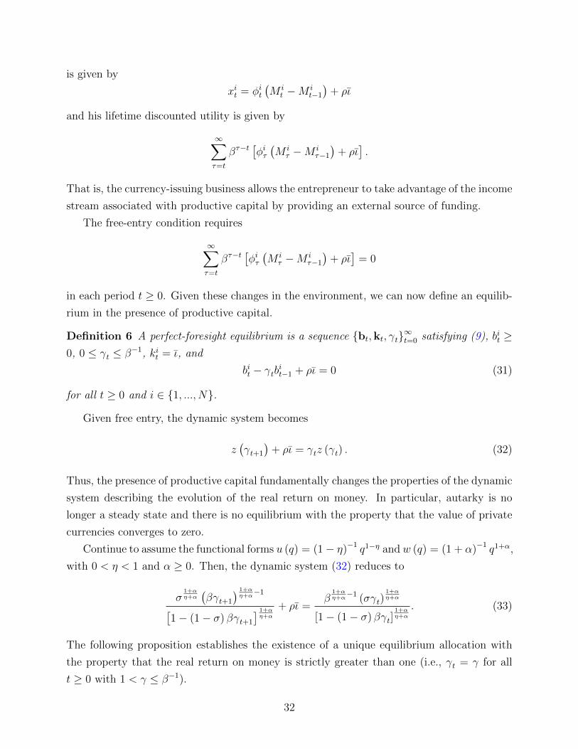
Definition 6 A perfect-foresight equilibrium is a sequence {bt,kt, γt}∞t=0 satisfying (9), bit ≥

0, 0 ≤ γt ≤ β−1, kit = ι, and

bit − γtbit−1 + ρι = 0 (31)

for all t ≥ 0 and i ∈ {1, ..., N}.

Given free entry, the dynamic system becomes

z(γt+1

)+ ρι = γtz (γt) . (32)

Thus, the presence of productive capital fundamentally changes the properties of the dynamic

system describing the evolution of the real return on money. In particular, autarky is no

longer a steady state and there is no equilibrium with the property that the value of private

currencies converges to zero.

Continue to assume the functional forms u (q) = (1− η)−1 q1−η and w (q) = (1 + α)−1 q1+α,

with 0 < η < 1 and α ≥ 0. Then, the dynamic system (32) reduces to

σ1+αη+α(βγt+1

) 1+αη+α−1[

1− (1− σ) βγt+1

] 1+αη+α

+ ρι =β

1+αη+α−1 (σγt)

1+αη+α

[1− (1− σ) βγt]1+αη+α

. (33)

The following proposition establishes the existence of a unique equilibrium allocation with

the property that the real return on money is strictly greater than one (i.e., γt = γ for all

t ≥ 0 with 1 < γ ≤ β−1).

32

Proposition 8 Suppose u (q) = (1− η)−1 q1−η and w (q) = (1 + α)−1 q1+α, with 0 < η < 1

and α ≥ 0. Then, there exists a unique equilibrium allocation with the property γt = γs for

all t ≥ 0 and 1 < γs ≤ β−1.

Proof. It can be shown that dγt+1/dγt > 0 for all γt > 0. When γt+1 = 0, we have

γt =(ρι)

η+α1+α

σβ1−η1+α + (ρι)

η+α1+α (1− σ) β

.

Because γt ∈[0, β−1

]for all t ≥ 0, a nonstationary solution would violate the boundary

condition. Thus, the unique solution is stationary, γt = γs for all t ≥ 0, and must satisfy

σ1+αη+α (βγs)

1+αη+α−1 + ρι [1− (1− σ) βγs]

1+αη+α = β

1+αη+α−1 (σγs)

1+αη+α

and(ρι)

η+α1+α

σβ1−η1+α + (ρι)

η+α1+α (1− σ) β

≤ γs ≤ 1

β.

The presence of productive capital results in the global determinacy of equilibrium under

free entry. Any belief implying a persistently declining value of private money is not consis-

tent with the equilibrium conditions when entrepreneurs issue currency to fund productive

projects. The existence of productive projects in the economy provides a fundamental value

for the entrepreneur’s currency-issuing business, which falsifies any privately held belief with

the property that the exchange value of an entrepreneur’s currency monotonically converges

to zero. Figure 6 plots the dynamic system (33) with α = .5, β = .9, η = .5, σ = .9, ρ = .15,

and ι = .5.

Also, the presence of productive capital implies a strictly positive real return on money

under free entry, reducing the opportunity cost of holding money for transaction purposes.

In a perfectly competitive environment, free entry implies that the gains from intertemporal

investment opportunities translate into a higher yield on privately issued currencies in the

form of a sustained deflation. As a result, the ensuing equilibrium allocation Pareto dominates

the allocation associated with price stability derived in the absence of productive capital.

Moreover, the equilibrium real return on money approaches the efficient upper bound β−1

as the technological rate of return on capital increases. Therefore, the unique equilibrium

allocation approaches the efficient allocation as the return on capital rises. In other words, a

purely private monetary arrangement is consistent with Friedman’s (1969) optimum quantity

of money when capital is sufficiently productive.

33

Figure 6: dynamic system (33)

To verify that a sustained deflation is consistent with individual optimization, note that

the free-entry condition implies

∞∑τ=t

βτ−t[φiτ(M i

τ −M iτ−1

)+ ρι

]= 0

at all dates t ≥ 0. Because consumption is nonnegative, we must have

φit(M i

t −M it−1

)+ ρι = 0

in every period t ≥ 0. If the currency issued by entrepreneur i is valued in equilibrium,

we must have M it < M i

t−1. Thus, the nominal supply of each brand must be monotonically

decreasing to be consistent with free entry. This means that, along the equilibrium trajectory,

an entrepreneur’s purchases exceed his sales in the CM, with the shortfall financed by the

proceeds from investment in the productive technology. Thus, the presence of productive

capital makes a sustained deflation feasible as an equilibrium outcome under free entry.

The implementation of the previously described allocation requires the enforcement of

the plan consistent with profit maximization. As we have seen, an entrepreneur makes pur-

chases that exceed his sales in the CM when his nominal supply is strictly decreasing. If an

entrepreneur deviated from this plan by retaining the proceeds from capital investments, he

34

would clearly be better off. Thus, it is necessary to punish entrepreneurs who opportunisti-

cally deviate from the plan consistent with individual optimization when the nominal supply

is strictly decreasing. In the absence of productive capital, the nominal supply consistent

with free entry is constant over time so that an opportunistic deviation is not an issue in the

baseline model without capital. The consequences of the absence of an enforcement mecha-

nism of the plan are an interesting avenue for future research, but go well beyond the scope

of this paper.

The following example illustrates these important properties of an economy with produc-

tive capital and competing private currencies.

Example 7 Suppose u (q) = 2√q and w (q) = q. In addition, assume σ → 1. In this case,

the dynamic system is given by

γt+1 = γ2t − β−1ρι ≡ f (γt) .

The unique fixed point in the range[0, β−1

]is

γs ≡ 1 +√

1 + 4β−1ρι

2

provided ρ ≤ 1−βιβ

. Because f ′ (γ) > 0 for all γ > 0 and 0 = f(√

β−1ρι)

, it follows that

γt = γs for all t ≥ 0 is the unique equilibrium trajectory. As we can see, the real return on

money is strictly greater than one. If we take the limit

ρ→ 1− βιβ

,

we find that the unique equilibrium allocation is socially efficient.

In our model, not only do the entrepreneurs have access to the technologies to produce

nonfalsifiable tokens and keep track of trading histories but they also have the opportunity

to invest in a productive project at each date. One can interpret an entrepreneur in our

framework as the owner of an internet platform (i.e., a productive project) that issues money

to be used for the purchase of goods through her platform. Thus, a monetary system with

the previously described properties is closer to reality than one might initially imagine. And

the desirable properties we have demonstrated serve as a useful guide to regulators, policy

makers, and others interested in the future of digital currencies.

Indeed, the result that when entrepreneurs can issue currency to fund socially productive

projects, a competitive monetary system is consistent with monetary stability and implements

35

an allocation that is arbitrarily close to the efficient allocation is a key finding of this paper.

This result vindicates Hayek’s proposal for the denationalization of money and it links our

research to the literature on the provision of liquidity by productive firms (Holmstrom and

Tirole, 2011, and Dang, Gorton, Holmstrom, and Ordonez, 2014).

The possibility of having a private monetary arrangement consistent with Friedman’s

optimum quantity of money has recently been studied by Monnet and Sanches (2015) and

Andolfatto, Berentsen, and Waller (2016). Monnet and Sanches (2015) characterize a mon-

etary arrangement in which privately issued debt claims circulate as a medium of exchange.

In their analysis, the debt claims are associated with an explicit promise by the issuer to

redeem them at some expected value. Andolfatto, Berentsen, and Waller (2016) study the

properties of a monetary arrangement in which an institution with the monopoly rights on the

economy’s physical capital issues claims that circulate as a medium of exchange. However,

these arrangements are fundamentally different from our analysis of currency competition.

8 Network Effects

Many discussions of currency competition highlight the importance of network effects.

See, for example, Halaburda and Sarvary (2015). To evaluate these network effects, let us

consider a version of the baseline model in which the economy consists of a countable infinity

of identical locations indexed by j ∈ {...,−2,−1, 0, 1, 2, ...}. Each location contains a [0, 1]-

continuum of buyers, a [0, 1]-continuum of sellers, and a countable infinity of entrepreneurs.

All agents have the same preferences and technologies as previously described. For simplicity,

we take the limit σ → 1 so that each buyer is randomly matched with a seller with probability

one and vice versa.

The main change from the baseline model is that sellers move randomly across locations.

Suppose that a fraction 1 − δ of sellers in each location j is randomly selected to move to

location j + 1 at each date t ≥ 0. Assume that the seller’s relocation status is publicly

revealed at the beginning of the decentralized market and that the actual relocation occurs

after the decentralized market closes.

We start by showing the existence of a symmetric and stationary equilibrium with the

property that the currency issued by an entrepreneur in location j circulates only in that

location. In this equilibrium, a seller who finds out he is going to be relocated from location

j to j+1 does not produce the DM good for the buyer in exchange for local currency because

he believes that currency issued in location j will not be valued in location j + 1. This belief

can be self-fulfilling so that currency issued in location j circulates only in that location. In

36

this case, the optimal portfolio choice implies the first-order condition

δu′ (q (m, t))

w′ (q (m, t))+ 1− δ =

1

βγit+1

for each currency i. Note that we have suppressed any superscript or subscript indicating the

agent’s location, given that we restrict attention to symmetric equilibria. Let q (γ) denote the

DM output as an implicit function of the real return γ. Then, the demand for real balances

in each location is given by

z(γt+1

)≡w(q(γt+1

))βγt+1

,

where γt+1 denotes the common rate of return across all valued currencies in a given location.

Because the market-clearing condition implies

N∑i=1

φitMit = z

(γt+1

),

the equilibrium sequence {γt}∞t=0 satisfies the law of motion

z(γt+1

)= γtz (γt)

and the boundary condition 0 ≤ γt ≤ β−1.

Suppose u (q) = (1− η)−1 q1−η and w (q) = (1 + α)−1 q1+α, with 0 < η < 1 and α ≥ 0.

Then, the dynamic system describing the equilibrium evolution of γt is given by

γ1+αη+α−1

t+1[1− (1− δ) βγt+1

] 1+αη+α

=γ

1+αη+α

t

[1− (1− δ) βγt]1+αη+α

(34)

and the boundary condition 0 ≤ γt ≤ β−1. The following proposition establishes the existence

of a stationary equilibrium with the property that privately issued currencies circulate locally.

Proposition 9 Suppose u (q) = (1− η)−1 q1−η and w (q) = (1 + α)−1 q1+α, with 0 < η < 1

and α ≥ 0. There exists a stationary equilibrium with the property that the quantity traded

in the DM is given by q (δ) ∈ (0, q∗) satisfying

δu′ (q (δ))

w′ (q (δ))+ 1− δ = β−1. (35)

In addition, q (δ) is strictly increasing in δ.

Proof. It is easy to show that the sequence γt = 1 for all t ≥ 0 satisfies (34). Then,

37

the solution to the optimal portfolio problem implies that the DM output must satisfy (35).

Because the term u′ (q) /w′ (q) is strictly decreasing in q, it follows that the solution q (δ) to

(35) must be strictly increasing in δ.

The previously described stationary allocation is associated with price stability across

all locations, but production in the DM occurs only in a fraction δ ∈ (0, 1) of all bilateral

meetings. Only a seller who is not going to be relocated is willing to produce the DM good in

exchange for locally issued currency. A seller who finds out he is going to be relocated does

not produce in the DM because the buyer can only offer him currencies that are not valued

in other locations.

Now we construct an equilibrium in which the currency issued by an entrepreneur in

location j circulates in other locations. To do so, we establish a currency-exchange system

similar to that of Cavalcanti, Erosa, and Temzelides (1999). Suppose the entrepreneurs in all

locations establish a currency-exchange system by which entrepreneur i in location j agrees

to retire the currency issued by entrepreneur i in location j − 1. In this case, the budget

constraint for entrepreneur i in each location is given by

xit + φitMit−1 = φitM

it .

In this equation, the term M it−1 refers to all currency of type i that is in circulation in a

given location before the centralized market opens. In a symmetric equilibrium, the same

amount of type-i currency that flowed from location j to j + 1 in the previous period flowed

into location j as relocated sellers moved across locations. As a result, M it−1 denotes the

beginning-of-period type-i circulation in a given location. Given the common knowledge of

a currency-exchange system, we build an equilibrium with the property that all sellers in a

given location accept locally issued currency because they believe that these currencies will

be valued in other locations. In this case, the optimal portfolio choice implies the first-order

conditionu′ (q (m, t))

w′ (q (m, t))=

1

βγit+1

for each currency i. Let q (γ) denote the DM output as an implicit function of the real return

γ. Then, the demand for real balances in each location is given by

z(γt+1

)≡w(q(γt+1

))βγt+1

.

38

Because the market-clearing condition implies

N∑i=1

φitMit = z

(γt+1

),

the equilibrium sequence {γt}∞t=0 satisfies the law of motion

z(γt+1

)= γtz (γt)

and the boundary condition 0 ≤ γt ≤ β−1.

Suppose u (q) = (1− η)−1 q1−η and w (q) = (1 + α)−1 q1+α, with 0 < η < 1 and α ≥ 0.

Then, the dynamic system describing the equilibrium evolution of γt is

γ1+αη+α−1

t+1 = γ1+αη+α

t (36)

and the boundary condition 0 ≤ γt ≤ β−1. The following proposition establishes the existence

of a stationary equilibrium with the property that locally issued currencies circulate in several

locations.

Proposition 10 Suppose u (q) = (1− η)−1 q1−η and w (q) = (1 + α)−1 q1+α, with 0 < η < 1

and α ≥ 0. There exists a stationary equilibrium with the property that the quantity traded

in the DM is given by q ∈ (q (δ) , q∗) satisfying

u′ (q)

w′ (q)= β−1. (37)

Proof. It is straightforward to show that the sequence γt = 1 for all t ≥ 0 satisfies (36).

Then, the solution to the optimal portfolio problem implies that the DM output must satisfy

(37). The quantities q and q (δ) satisfy

u′ (q)

w′ (q)= δ

u′ (q (δ))

w′ (q (δ))+ 1− δ.

Because δ ∈ (0, 1), we must have q > q (δ) as claimed.

Because q > q (δ), the allocation associated with the currency-exchange system Pareto

dominates the allocation associated with the local circulation of private currencies. Thus, we

conclude that, in the presence of currency-exchange systems, the presence of network effects

may be less relevant than argued by the previous literature.

39

9 Conclusion

In this paper, we have shown how a system of competing private currencies can work. Our

evaluation of such a system is nuanced. While we offer glimpses of hope for it by showing

the existence of stationary equilibria that deliver price stability, there are plenty of other less

desirable equilibria. And even the best equilibrium does not deliver the socially optimum

amount of money. Furthermore, at this stage of the research, we do not have any argument

to forecast the empirical likelihood of each of these equilibria.

Although a system of competing currencies does not necessarily imply efficiency and

stability, we have identified the characteristics of an efficient and stable private monetary

arrangement under free entry, given that our framework is sufficiently flexible to consider

relevant extensions of the baseline model. As we have seen, the introduction of productive

capital fundamentally changes the properties of the model, implying the existence of a unique

equilibrium allocation that can be arbitrarily close to the efficient allocation depending on

the technological rate of return on capital. This result is illuminating as it identifies the

characteristics of a socially beneficial private monetary system.

We have, nevertheless, just scratched the surface of the study of private currency compe-

tition. Many topics, including the analysis of the different degrees of moneyness of private

currencies (including interest-bearing assets and redeemeable instruments), the role of pos-

itive transaction costs among different currencies, the entry and exit of entrepreneurs, the

possibility of market power by currency issuers, or the consequences of the lack of enforce-

ability of contracts are some of the avenues for future research that we hope to tackle shortly.

40

References

Andolfatto, D., A. Berentsen, and C. Waller (2016): “Monetary policy with asset-

backed money,” Journal of Economic Theory, forthcoming.

Antonopoulos, A. M. (2015): Mastering Bitcoin. O’Reilly.

Araujo, L., and B. Camargo (2008): “Endogenous supply of fiat money,” Journal of

Economic Theory, 142(1), 48–72.

Aruoba, S., G. Rocheteau, and C. Waller (2007): “Bargaining and the value of

money,” Journal of Monetary Economics, 54(8), 2636–2655.

Berentsen, A. (2006): “On the private provision of fiat currency,” European Economic

Review, 50(7), 1683–1698.

Bohme, R., N. Christin, B. Edelman, and T. Moore (2015): “Bitcoin: economics,

technology, and hovernance,” Journal of Economic Perspectives, 29(2), 213–38.

Cavalcanti, R. d. O., A. Erosa, and T. Temzelides (1999): “Private money and

reserve management in a random-matching model,” Journal of Political Economy, 107(5),

929–945.

(2005): “Liquidity, money creation and destruction, and the returns to banking,”

International Economic Review, 46(2), 675–706.

Cavalcanti, R. d. O., and N. Wallace (1999): “Inside and outside money as alternative

media of exchange,” Journal of Money, Credit and Banking, 31(3), 443–57.

Chiu, J., and T.-N. Wong (2014): “E-Money: efficiency, stability and optimal policy,”

Staff Working Papers 14-16, Bank of Canada.

Chuen, D. L. K. (2015): Handbook of Digital Currency: Bitcoin, Innovation, Financial

Instruments, and Big Data. Elsevier.

Dang, T. V., G. Gorton, B. Holmstrom, and G. Ordonez (2014): “Banks as secret

keepers,” Working Paper 20255, National Bureau of Economic Research.

Friedman, M. (1969): “The optimum quantity of money,” in The Optimum Quantity of

Money and Other Essays. Aldine Publishing Company.

Friedman, M., and A. J. Schwartz (1986): “Has government any role in money?,”

Journal of Monetary Economics, 17(1), 37–62.

41

Gorton, G. (1989): “An Introduction to Van Court’s Bank Note Reporter and Counterfeit

Detector,” Working paper, University of Pennsylvania.

Greco, T. H. (2001): Money: Understanding and Creating Alternatives to Legal Tender.

Chelsea Green Publishing.

Halaburda, H., and M. Sarvary (2015): Beyond Bitcoin: The Economics of Digital

Currencies. Palgrave Macmillan.

Hayek, F. (1999): “The denationalization of money: An analysis of the theory and practice

of concurrent currencies,” in The Collected Works of F.A. Hayek, Good Money, Part 2, ed.

by S. Kresge. The University of Chicago Press.

Hendrickson, J. R., T. L. Hogan, and W. J. Luther (2016): “The political economy

of Bitcoin,” Economic Inquiry, forthcoming.

Holmstrom, B., and J. Tirole (2011): Inside and Outside Liquidity. The MIT Press.

Kareken, J., and N. Wallace (1981): “On the indeterminacy of equilibrium exchange

rates,” The Quarterly Journal of Economics, 96(2), 207–222.

Klein, B. (1974): “The competitive supply of money,” Journal of Money, Credit and Bank-

ing, 6(4), 423–53.

Lagos, R., and R. Wright (2003): “Dynamics, cycles, and sunspot equilibria in ’genuinely

dynamic, fundamentally disaggregative’ models of money,” Journal of Economic Theory,

109(2), 156–171.

(2005): “A unified framework for monetary theory and policy analysis,” Journal of

Political Economy, 113(3), 463–484.

Martin, A., and S. L. Schreft (2006): “Currency competition: A partial vindication of

Hayek,” Journal of Monetary Economics, 53(8), 2085–2111.

Monnet, C. (2006): “Private Versus public money,” International Economic Review, 47(3),

951–960.

Monnet, C., and D. R. Sanches (2015): “Private money and banking regulation,” Jour-

nal of Money, Credit and Banking, 47(6), 1031–1062.

Narayanan, A., J. Bonneau, E. Felten, A. Miller, and S. Goldfeder (2016):

Bitcoin and Cryptocurrency Technologies. Princeton University Press.

42

Obstfeld, M., and K. Rogoff (1983): “Speculative hyperinflations in maximizing mod-

els: Can we rule them out?,” Journal of Political Economy, 91(4), 675–87.

Sanches, D. (2016): “On the inherent instability of private money,” Review of Economic

Dynamics, 20, 198–214.

Selgin, G. A., and L. H. White (1994): “How would the invisible hand handle money?,”

Journal of Economic Literature, 32(4), 1718–1749.

Tullock, G. (1975): “Competing monies,” Journal of Money, Credit and Banking, 7(4),

491–97.

von zur Gathen, J. (2015): CryptoSchool. Springer.

Wallace, N. (2001): “Whither monetary economics?,” International Economic Review,

42(4), 847–69.

White, L. H. (1995): Free Banking in Britain: Theory, Experience and Debate, 1800-1845.

Institute of Economic Affairs, second (revised and extended) edn.

Williamson, S. D. (1999): “Private money,” Journal of Money, Credit and Banking, 31(3),

469–91.

43