NBER WORKING PAPER SERIES

INNOVATION, FIRM DYNAMICS, AND INTERNATIONAL TRADE

Andrew AtkesonAriel Burstein

Working Paper 13326http://www.nber.org/papers/w13326

NATIONAL BUREAU OF ECONOMIC RESEARCH1050 Massachusetts Avenue

Cambridge, MA 02138August 2007

We thank Daron Acemoglu, Jonathan Eaton, Kei-Mu Yi, Marc Melitz, Natalia Ramondo, EstebanRossi-Hansberg, Nancy Stokey, and seminar participants in various places for very useful comments.The views expressed herein are those of the author(s) and do not necessarily reflect the views of theNational Bureau of Economic Research.

© 2007 by Andrew Atkeson and Ariel Burstein. All rights reserved. Short sections of text, not to exceedtwo paragraphs, may be quoted without explicit permission provided that full credit, including © notice,is given to the source.

Innovation, firm dynamics, and international tradeAndrew Atkeson and Ariel BursteinNBER Working Paper No. 13326August 2007JEL No. F1,L11,L16,O3

ABSTRACT

We present a general equilibrium model of the decisions of firms to innovate and to engage in internationaltrade. We use the model to analyze the impact of a reduction in international trade costs on firms' processand product innovative activity. We first show analytically that if all firms export with equal intensity,then a reduction in international trade costs has no impact at all, in steady-state, on firms' investmentsin process innovation. We then show that if only a subset of firms export, a decline in marginal tradecosts raises process innovation in exporting firms relative to that of non-exporting firms. This reallocationof process innovation reinforces existing patterns of comparative advantage, and leads to an amplifiedresponse of trade volumes and output over time. In a quantitative version of the model, we show thatthe increase in process innovation is largely offset by a decline in product innovation. We find that,even if process innovation is very elastic and leads to a large dynamic response of trade, output, consumption,and the firm size distribution, the dynamic welfare gains are very similar to those in a model with inelasticprocess innovation.

Andrew AtkesonBunche Hall 9381Department of EconomicsUCLABox 951477Los Angeles, CA 90095-1477and NBERandy@atkeson.net

Ariel BursteinDepartment of EconomicsBunche Hall 8365Box 951477UCLALos Angeles, CA 90095-1477and NBERarielb@econ.ucla.edu

1. Introduction

Over the past several decades, there has been a striking growth in the share of international

trade in output, both for the US economy and for the world as a whole. How has this

expansion of opportunities for international trade changed firms’ incentives to engage in

innovative activities?

In this paper, we present a simple general equilibrium model of the decisions of firms to

innovate and to participate in international trade. Motivated by the observation that there

is large heterogeneity in export behavior across firms even within narrowly defined sectors,

recent research in international trade has modeled comparative advantage as an attribute of

the firm (see, for example, Melitz 2003 and Bernard, Jensen, Eaton, and Kortum 2003). In

these models, each firm has a stock of some firm specific factor that determines its current

profit opportunities. Examples of this firm specific factor include productivity, managerial

skill, product quality, or brand name. Our model includes two forms of innovation: innova-

tion to increase the stock of this firm specific factor in an existing firm — process innovation,

and innovation to create new firms with a new initial stock of the firm specific factor —

product innovation. We use the model to study the dynamic gains from trade that arise as

process and product innovation respond to a decline in the costs of international trade.

We start our analysis of the impact of a reduction in the costs of international trade

on innovation with a stark analytical result. We show in our model that if all firms export

(so the fixed costs of international trade are zero) then, in general equilibrium, a decrease

in the marginal costs of international trade has no impact at all, in steady-state, on firms’

process innovation decisions and hence no impact on aggregate productivity and output over

an above the impact of this trade cost reduction on the volume of trade and production in

a version of the model that abstracts from process innovation.

The intuition for this result in our model is as follows. If all firms export, a reduction

in the marginal costs of international trade changes the profit opportunities of all firms by

the same proportion. The returns to process innovation are proportional to firm profits, so

a reduction in the marginal costs of international trade also changes the returns to process

innovation by the same proportion for all firms. In general equilibrium with free entry, the

expected profits of starting a new firm and the cost of innovative inputs must rise by the same

amount to ensure that there are zero profits to product innovation. Because the reduction

in trade costs affects the opportunities of all firms proportionally, this free entry condition

2

implies that the ratio of the returns to process innovation to the cost of innovative inputs

remains unchanged for all firms. Hence, the equilibrium process innovation decisions are left

unchanged.

This result implies that when all firms export, our model has steady-state implications for

the impact of changes in marginal trade costs on product innovation closely related to several

existing results in the literature building on the work of Krugman (1980) and Grossman and

Helpman (1991). The models in this literature typically abstract from process innovation

within ongoing firms and focus instead only on product innovation measured in terms of the

introduction of new goods. Our result also echoes the findings of Eaton and Kortum (2001).

They find the same result that changes in the costs of international trade have no impact

on innovative effort in a model of quality ladders embedded in a multi-country Ricardian

model of international trade, with a research sector that produces new ideas randomly across

goods. Our result differs from theirs in that in our model, process innovation is directed

toward reducing the firm’s marginal cost of producing a specific product and firms do not

compete over technological leadership in producing any particular product.

Our analytical result that changes in the costs of trade have no impact on firm level

process innovation holds only if all firms have equal exposure to opportunities for interna-

tional trade. In the data, however, firms vary greatly in their participation in international

trade – exports are highly concentrated among large firms. Here we build on the insight of

Melitz (2003) and add to our model a fixed cost of trade at the firm level so that only the

more productive (and hence larger) firms choose to export. In this case, a reduction in the

marginal costs of trade leads in general equilibrium to an increase in profits of exporting firms

relative to the profits of firms that do not export. We show analytically in our model that a

reduction in marginal trade costs leads in equilibrium to an increase in process innovation in

exporting firms relative to that in firms that do not export. Hence, over time, this reduction

in trade costs leads to an amplification of the initial reallocation effects of a decrease in

trade costs – exporting firms grow over time and increase their exports while firms that do

not export shrink. In other words, this reallocation of process innovation amplifies existing

patterns of comparative advantage and amplifies the response of trade and output over time.

We then develop a quantitative version of our model and show that it reproduces many

salient features of the U.S. data on firm dynamics and export behavior. We use this model

to assess the impact of a reduction in the costs of international trade on firms’ innovative

3

activity and the associated dynamic gains from trade. One challenge we face in making

our model quantitative is to infer how elastic process innovation effort is to changes in the

incentives to innovate. If investments in process innovation are highly inelastic, then the

dynamic responses of exports, output, consumption and the firm size distribution do not

vary substantially from those of a model that abstracts from endogenous process innovation.

In contrast, if process innovation is highly elastic, then these dynamic responses can be

quite large. We examine our model’s implications for a wide range of this process innovation

elasticity parameter.

We find two main results. Our first result is that in response to a decline in marginal

trade costs, the increase in process innovation is largely offset by a decline in product inno-

vation, and these changes in innovation are larger the more elastic is process innovation.1

This result follows from the free entry condition governing the creation of new firms. In

equilibrium, prices and entry have to adjust following a decline in international trade costs

so as to leave the value of starting a new firm equal to the entry cost. To the extent that

a decline in international trade cost increases process innovation and hence productivity in

large exporting firms, it drives up wages and drives down the value of entrants, which tend

to be small non-exporting firms. Hence, entry falls to restore the free entry condition.

Our second result is that consideration of elastic process innovation does not substantially

alter the dynamic welfare implications of a reduction in international trade costs. We find

that, even when elastic process innovation leads to very large steady state changes in export

volumes, output, consumption, and substantial changes in the firm size distribution, the dy-

namic welfare gains from trade are only slightly higher than the gains achieved with inelastic

process innovation. This finding follows because process innovation is an investment – the

long-run productivity gains that result from increased innovation require an investment of

current resources – and, in our model, the output gains from this investment come only

slowly. We show in particular that the transition in our economy from one steady-state to

another takes a lot of time.

Our model is closely related to several papers in the literature. If we assume that firms’

process innovation choices are inelastic, then our model is a variant of Hopenhayn’s (1992)

model in which firms’ experience exogenous random shocks to their productivity. In this case,

1Baldwin and Robert Nicoud (2007) present a related result, but our finding differs from theirs in thatwe find that changes in process and product innovation largely offset: the decline in product innovation islarger the more elastic is the response of process innovation.

4

our model is specifically an open economy version of the model of firm dynamics in Luttmer

(2006) and hence is quite similar to Irarrazabal and Opromolla (2006). Our inclusion of fixed

and marginal costs of exporting also follows Melitz (2003) and Bernard, Eaton, Jensen, and

Kortum (2003), among many others. We study such a version of our model as a benchmark

to show that it can reproduce many of the same features of the US data on firm dynamics,

the firm size distribution, and export decisions studied in these papers.2 One of the most

important of these features is Gibrat’s Law – the observation that, at least for large firms,

firm growth is independent of firm size.

Our model of firms’ process innovation follows Griliches’ (1979) knowledge capital model

of firm productivity, and the work of Ericson and Pakes (1995). The assumption that the

fruits of innovative activity are stochastic in our model means it can account for simultaneous

growth and decline, and entry and exit of firms in steady-state.3 Our model is also related

to Bustos (2005), who provides empirical support (using firm level data from Argentina) for

a model of trade and heterogeneous firms in which exporters choose to pay a one-time fixed

cost to upgrade their technology. It is also related to the work of Costantini and Melitz

(2007), that studies how the dynamics of trade liberalizations shapes the pace of one-time

technology upgrading and productivity improvements across firms.

Our paper complements the work of Klette and Kortum (2004) and Lentz and Mortensen

(2006) in constructing a model of innovation that abstracts from strategic interactions across

firms and is also consistent with data on firm dynamics. While their framework is a quality

ladders model a la Grossman and Helpman (1991) where firms engage in undirected inno-

vation and their dynamics are governed by creative destruction, ours is a model in which

monopolistically competitive firms engage in product innovation and process innovation to

shape the stochastic process of their production cost.

The paper is organized as follows. Section 2 presents our model and Section 3 charac-

terizes the equilibrium. Section 4 describes the analytic result that if all firms export then

a change in trade costs has no effect on the firms’ process innovation decisions and char-

acterizes the impact of a change in trade costs on product innovation. Section 5 examines

analytically the reallocation of process innovation that occurs in response to a change in

trade costs when not all firms export. Section 6 discusses the implications for firm growth.

2In related work, Alessandria and Choi (2007) study the welfare gains of trade in a dynamic version ofMelitz’ model that abstracts from process innovation.

3Doraszelski and Jaumandreu (2006) estimate a Griliches’ knowledge capital model in which innovativeinvestments within the firm also lead to stochastic productivity improvements.

5

Section 7 presents the quantitative model and describes how we calibrate the model to match

salient features of the US data on firm dynamics and export behavior. Section 8 presents

the model’s quantitative implications for the response of innovation, output, consumption,

and welfare to a decline in trade costs, both across steady states and along the transition.

Section 9 concludes. An Appendix includes the characterization of equilibrium, proofs, and

solution methods.

2. The Model

Time is discrete and labelled t = 0, 1, 2, . . . . There are two countries: home and foreign. Vari-

ables pertaining to the foreign country are denoted with a star. Households in each country

are endowed with L units of time. Production in each country is structured as follows. There

is a single final nontraded good that can be consumed or used in innovative activities, a con-

tinuum of differentiated intermediate goods that are produced and can be internationally

traded subject to a fixed and a variable trade cost, and a nontraded intermediate good that

we call the research good. This research good is produced using a combination of final output

and labor, and is used to pay the costs associated with both process and product innova-

tion, as well as the fixed costs of exporting. The productivities of the firms producing the

differentiated intermediate goods are determined endogenously through equilibrium process

innovation, and the measure of differentiated intermediate goods produced in each country

is determined endogenously through product innovation. To simplify the presentation of the

analytical results in the paper, the benchmark model abstracts from fixed operating costs

(that give rise to endogenous exit), and time varying fixed export costs (to account for the

extent of firm switching between exporting and non-exporting status). These considerations

are introduced in the quantitative model in Section 7.

Households in the home country have preferences of the formP∞

t=0 βt log(Ct), where Ct

is the consumption of the home final good at date t. Households in the foreign country have

preferences of the same form over consumption of the foreign final good C∗t . Each household

in the home country faces an intertemporal budget constraint of the form

∞Xt=0

Qt (PtCt −WtL) ≤ W̄ , (2.1)

where Qt are intertemporal prices, Wt is the wage in the home country, Pt is the price of the

home final good, Ct is the household’s consumption, and W̄ is the initial stock of assets held

6

by the household. Households in the foreign country face similar budget constraints with

the same intertemporal prices Qt and wages, prices, and assets all labelled with stars.

Intermediate goods are differentiated products each produced by heterogeneous firms in-

dexed by z, which indicates their productivity. A firm in the home country with productivity

index z has productivity equal to exp(z)1/(ρ−1) and produces output yt(z) with labor lt(z)

according to the CRS production technology

yt(z) = exp(z)1/(ρ−1)lt(z). (2.2)

We rescale firm productivity using the exponent 1/ (ρ− 1) so that, as explained below, laborand profits are proportional to exp (z).

The output of this firm can be used in the production of the home final good, with the

quantity of this domestic absorption denoted at(z). Alternatively, some of this output can

be exported to the foreign country to be used in the production of the foreign final good.

International trade is subject to both fixed and iceberg type costs of exporting. The fixed,

per-period cost of exporting in terms of the research good is denoted by nx. The iceberg type

marginal cost of exporting is denominated in terms of the intermediate good being exported.

The firm must export Da∗t (z) units of output, with D ≥ 1, to have a∗t (z) units of outputarrive in the foreign country for use in the production of the foreign final good.

Let xt (z) ∈ {0, 1} be an indicator of the export decision of home firms with productivityindex z (it is 1 if the firm exports and 0 otherwise). Then, feasibility requires that

at(z) + xt(z)Da∗t (z) = yt(z) , (2.3)

and that xt (z)nx units of the research good be used to pay fixed costs of exporting.

A firm in the foreign country with productivity index z has the same production tech-

nology, with output denoted y∗t (z), labor l∗t (z), and domestic absorption b∗t (z). Exports to

the home country, bt (z), are subject to both fixed and marginal costs and hence feasibility

requires that x∗t (z)Dbt(z) + b∗t (z) = y∗t (z), and that x∗t (z)nx units of the foreign research

good be used to pay the fixed costs of exporting.

The home final good is produced from home and foreign intermediate goods with a

constant returns production technology of the form

Yt =

∙Zat (z)

1−1/ρ dMt(z) +

Zx∗t (z)bt (z)

1−1/ρ dM∗t (z)

¸ρ/(ρ−1), (2.4)

7

where Mt(z) is the measure of operating firms in the home country with productivity less

than or equal to z, andM∗t (z) the corresponding measure in the foreign country. Production

of the final good in the foreign country is defined analogously. It will be useful below to

distinguish between the total measure of operating firms given by Nt = Mt(∞), and thedistribution of z across operating firms which has a cumulative distribution function given

by Mt(z)/Nt.

The final good in the home country is produced by competitive firms that choose output

Yt and inputs at(z) and bt(z) subject to (2.4) to maximize profits taking prices Pt, pat(z),

pbt(z), export decisions xt(z), x∗t (z), and measures of operating intermediate goods firms Mt

and M∗t as given. Standard arguments give that equilibrium prices must satisfy

Pt =

∙Zpat (z)

1−ρ dMt(z) +

Zx∗t (z)pbt (z)

1−ρ dM∗t (z)

¸1/(1−ρ), (2.5)

and quantitiesat(z)

Yt=

µpat(z)

Pt

¶−ρand

bt(z)

Yt=

µpbt(z)

Pt

¶−ρ. (2.6)

Analogous equations hold for prices and quantities in the foreign country.

The research good in the home country is produced with a constant returns to scale

production technology F that uses Xt units of the home final good and Lmt units of labor to

produce Ymt units of the research good according to Ymt = F (Xt, Lmt). As is standard, the

equilibrium price of the home research good, denoted by Wmt, is given as a function of the

price of the home final good Pt and the home wage Wt, by the unit cost function associated

with the production function F. We write this cost function Wmt = Wm(Pt,Wt). Likewise,

in the foreign country we have Y ∗mt = F (X∗t , L

∗mt) and W ∗

mt =Wm(P∗t ,W

∗t ).

Intermediate goods firms in each country are monopolistically competitive. A home firm

with productivity exp(z)1/(ρ−1) faces a static profit maximization problem of choosing labor

input lt(z), prices pat(z), p∗at(z), quantities at(z), a∗t (z), and whether or not to export xt (z),

to maximize current period profits taking as given wages for workers Wt, the price of the

home research good Wmt, and prices and output of the final good in both countries Pt, P∗t ,

Yt, and Y ∗t . This problem is written

Πt(z) = maxy,l,pa,p∗a,a,a∗,x∈{0,1}

paa+ xp∗aa∗ −Wtl −Wmtxnx (2.7)

subject to (2.2), (2.3), and the demand functions

a =

µpaPt

¶−ρYt and a∗ =

µp∗aP ∗t

¶−ρY ∗t . (2.8)

8

Productivity at the firm level evolves over time depending both on idiosyncratic produc-

tivity shocks hitting the firm and on the level of investment in productivity improvements

undertaken within the firm. We model the evolution of firm productivity as follows. At the

beginning of each period t, every existing firm has probability δ of exiting exogenously, and

corresponding probability 1− δ of surviving to produce. A surviving firm with current pro-

ductivity exp(z)1/(ρ−1), and that invests H (z, p) = h exp (z) c (p) units of the research good

in improving its productivity in the current period t, has probability p of having productivity

exp(z + s)1/(ρ−1) and probability 1 − p of having productivity exp(z − s)1/(ρ−1) in the next

period t+1.We assume that c (p) is increasing and convex in p, and h is a positive constant.

In the next sections, we show that this form of H (z, p) allows us to obtain analytical results

for process innovation.

With this evolution of firm productivity, the expected discounted present value of profits

for the firm satisfies the Bellman equation

Vt(z) = maxp∈[0,1]

Πt(z)−WmtH (z, p) + (1− δ)Qt+1

Qt[pVt+1(z + s) + (1− p)Vt+1(z − s)] . (2.9)

Let pt(z) denote the optimal choice of investment in improving productivity in the problem

(2.9). We refer to pt(z) as the process innovation decision of the firm. Note that if the

time period is small, our binomial productivity process approximates a geometric Brownian

motion in continuous time (as in Luttmer 2006) in which the firm controls the drift of this

process through investments of the research good.

New firms (or new products) are created with investments of the research good. Invest-

ment of ne units of the research good in period t yield a new firm in period t+1 with initial

productivity exp(z)1/(1−ρ) drawn from a distribution over z given by G. New firms are not

subject to exogenous exit in their entering period. In any period in which there is entry of

new firms, free entry requires that

Wmtne =Qt+1

Qt

ZVt+1(z)dG. (2.10)

LetMet denote the measure of new firms entering in period t, that start producing in period

t+1. The analogous Bellman equation holds for the foreign firms as well. We refer toMet as

the product innovation decision as this is the mechanism through which new differentiated

products are produced.

Feasibility requires that for the final good

Ct +Xt = Yt (2.11)

9

in the home country and the analogous constraint holds in the foreign country. The feasibility

constraint on labor in the home country is given byZlt(z)dMt(z) + Lmt = L , (2.12)

and likewise in the foreign country. The feasibility constraint on the research good in the

home country is

Metne +

Z[xt (z)nx +H (z, pt (z))] dMt(z) = F (Xt, Lmt) , (2.13)

and likewise in the foreign country.

The evolution of Mt(z) over time is determined by the exogenous probability of exit

δ, the decisions of operating firms to invest in their productivity pt(z), and the measure of

entering firms in period t−1,Met−1. The measure of operating firms in the home country with

productivity less than or equal to z0, denoted byMt+1(z0), is equal to the sum of three inflows:

new firms founded in period t, firms continuing from period t that draw positive productivity

shocks (and hence had productivities lower than z0 − s in period t), and firms continuing

from period t that draw negative productivity shocks (and hence had productivities below

z0 + s in period t). We write this as follows:

Mt+1(z0) = G(z0)Met + (1− δ)

Z z0−s

−∞pt(z)dMt(z) + (1− δ)

Z z0+s

−∞(1− pt(z))dMt(z) . (2.14)

The evolution of M∗t (z) for foreign firms is defined analogously.

We assume that the households in each country own those firms that initially exist at

date 0. Thus we require that the initial assets of the households in both countries adds up

to the total value of these firms

W̄ + W̄ ∗ =

ZV0(z)dM0(z) +

ZV ∗0 (z)dM

∗0 (z) . (2.15)

An equilibrium in this economy is a collection of sequences of prices and wages {Qt, Pt, P∗t ,

Wt,W∗t ,Wmt,W

∗mt, pat(z), p

∗at(z), pbt(z), p

∗bt(z)} a collection of sequences of quantities {Yt, Y ∗t ,

Ct, C∗t ,Xt,X

∗t , Lmt, L

∗mt, at(z), a

∗t (z), bt(z), b

∗t (z), lt(z), l

∗t (z)} initial assets W̄ , W̄ ∗, and a col-

lection of sequences of firm value functions and profit, export, and investment decisions

{Vt(z), V ∗t (z), V ot (z), V

o∗t (z),Πt(z),Π

∗t (z), xt(z), x

∗t (z), pt(z), p

∗t (z)} together with measures of

operating and entering firms {Mt(z),Met,M∗t (z),M

∗et} such that household in each country

are maximizing their utility subject to their budget constraints, intermediate goods firms

10

in each country are maximizing within period profits, final goods firms in each country are

also maximizing profits, all of the feasibility constraints are satisfied, and the measures of

operating firms evolve as described above.

A steady-state of our model is an equilibrium in which all of the variables are constant.4

In what follows, we omit time subscripts when discussing steady-states.

In some sections of the paper we focus our attention on equilibria that are symmetric

in the following sense. First, we assume that the distribution of initial assets is such that

expenditure is equal across countries at date 0 and hence in every period. Second, we assume

that each country starts with the same distribution of operating firms by productivity and

hence, because prices and wages are equal across countries, continue to have the same dis-

tribution of operating firms by productivity in each subsequent period. In such a symmetric

equilibrium, we have Yt = Y ∗t , Pt = P ∗t , and Wt/Pt =W ∗t /P

∗t .

3. Characterizing Equilibrium

We start with an analysis of the static profit maximization problem (2.7) for an operating firm

in the home country. All firms choose a constant markup over marginal cost, so equilibrium

prices are given by

pat(z) =ρ

ρ− 1Wt

exp(z)1/(ρ−1), and p∗at(z) =

ρ

ρ− 1DWt

exp(z)1/(ρ−1). (3.1)

The production employment of home firms is given by

lt(z) =

µρ− 1ρWt

¶ρ £(Pt)

ρ Yt + xt (z) (P∗t )

ρ Y ∗t D1−ρ¤ exp(z). (3.2)

Note that (3.2) implies that there is a simple relationship between the productivity index

exp (z) and firm size measured as workers employed in production of output for domestic con-

sumption. In contrast, there is no relationship between productivity in the model, measured

as exp(z)1/(ρ−1) and standard measures of labor productivity. This is because the average

productivity of workers in the firm (measured as sales per worker) is given by ρWt/(ρ− 1),and hence is constant across firms. Differences in productivity across firms in the model,

measured by exp(z)1/(ρ−1), are manifest in measures of firm size and not in measures of labor

4Since firms in our model grow endogenously through process innovation, there are parameter values forour model in which a steady-state does not exist. Under such parameter values, the equilibrium has no entryand a vanishing set of firms growing endogenously. We focus in the remainder of the paper on cases withpositive steady-state entry.

11

productivity.5 Hence, firms’ innovation decisions, pt(z), together with the stochastic shocks

to firm productivity and firms’ decisions to export determine the dynamics of firm size and

the long run distribution of firms by size in our economy.

Home firms have variable profits Πdt exp(z) on their home sales, with

Πdt =(Wt)

1−ρ (Pt)ρ Yt

ρρ (ρ− 1)1−ρ, (3.3)

and variable profits Πxt exp(z) on their foreign sales, with

Πxt =(Wt)

1−ρ (P ∗t )ρ Y ∗t

ρρ (ρ− 1)1−ρD1−ρ. (3.4)

Therefore, there is a cutoff firm productivity index z̄xt such that firms with productivity index

below z̄xt do not export and those with productivity index above z̄xt do export. Hence, we

have that firms’ static profits are given by

Πt(z) = Πdt exp (z) + max (Πxt exp (z)−Wmtnx, 0) . (3.5)

The decision of a firm to invest research goods in improving productivity, if interior, must

satisfy the first order condition

Wmt∂

∂pH (z, p) = (1− δ)

Qt+1

Qt[Vt+1(z + s)− Vt+1(z − s)] . (3.6)

This first order condition must satisfy the obvious inequality if the optimal choice of pt(z) is

equal to either 0 or 1. We discuss the implications of this first order condition (3.6) for the

impact of changes in the costs of trade on process innovation in the next several sections.

In Appendix 1, we describe the aggregate equilibrium conditions of the model.

4. Trade and innovation when all firms export

In this section we show that in an economy with no fixed costs of international trade, once and

for all changes in the marginal costs of trade have no impact at all on the incentives of firms

in steady-state to engage in process innovation. This result holds in general equilibrium

because, in an economy in which every firm exports, the increased incentives to innovate

5Our model gives this stark result because intermediate goods producing firms choose a constant markupof price over marginal cost. Note that the presence of fixed costs of production, if counted as workers, canonly generate differences in value-added per worker for small firms. Bernard, Eaton, Jensen, and Kortum(2003) develop a model in which the markup that firms charge rises with size and hence measured laborproductivity rises with firm size.

12

resulting from the increase in profits that come from a reduction in marginal trade costs are

exactly offset by an increase in the cost of the research good necessary for innovation. This

offsetting change in the cost of the research good is required by the zero-profit condition

associated with product innovation. As a result, the optimal process innovation decision of

all firms is unchanged. We also discuss the impact of changes in the marginal cost of trade

on product innovation in the steady-state of our model.

We state our main result in the following proposition

Proposition 1: Consider two different world economies, each consisting of two countries

as described above, with no fixed costs of trade (nx = 0). Let the marginal cost of trade

be D ≥ 1 in the first world economy and D0 6= D in the second world economy. Then, the

process innovation decisions of firms in a steady-state in both economies are identical in that

p(z) = p0(z) for all productivities z.

Proof: First observe that if all firms export, then from (3.3) and (3.4), variable profits of

home firms are directly proportional to exp(z) in that Π(z) = Π exp(z), where Π = Πd+Πx.

The analogous result is also true for firms in the foreign country. In a steady-state, all

equilibrium prices and value functions are constant and the interest rate is constant at 1/β.

Hence, if we impose steady-state and divide the firms’ Bellman equation given in (2.9) by

the steady-state price of the research good Wm, we can re-write this Bellman equation as

w(z) = maxp∈[0,1]

Π

Wmexp(z)−H (z, p) + (1− δ)β [pw(z + s) + (1− p)w(z − s)] . (4.1)

Standard arguments give that this Bellman equation has a unique solution w(z) correspond-

ing to any fixed value of Π/Wm. In addition, the solution w(z) is strictly increasing in

Π/Wm. We can regard the optimal choice of p(z) implied by this Bellman equation as the

optimal process innovation decision corresponding to a fixed ratio Π/Wm of variable profits

to innovation costs.6

Similarly, if we impose steady-state and divide the zero-profit condition (2.10) by the

steady-state price of the research good Wm, we can rewrite this condition as

ne = β

Zw(z)dG . (4.2)

6To ensure that this value function w (z) is well defined, we need that for all p ∈ [0, 1], either (i)β (1− δ) [p exp (s) + (1− p) exp (−s)] < 1 or (ii) Π/Wm − c (p) < 0. The first condition requires that theexpected growth of firm profits is less than the interest rate. If this is not satisfied, the second conditionrequires that the static profits of choosing such a high growth rate be negative.

13

We see from this scaled version of the free entry condition that the ratio of the discounted

expected value of profits from starting a new firm to the price of the research good must

be fixed at ne in any equilibrium in which there is entry. In a steady-state, the ratio of the

discounted expected value of profits from starting a new firm to the price of the research

good is strictly increasing in Π/Wm. Thus, since there is entry in a steady-state, there is

a unique value of Π/Wm consistent with equilibrium. The equilibrium process innovation

decisions of home firms in steady-state are thus independent of the parameter D. Clearly,

the analogous results hold for foreign firms. Q.E.D.

Our proof of Proposition 1 relies on our assumption that all innovation activities use the

same research good. If different inputs were required for product and process innovation,

then a change in trade costs might affect the relative price of the inputs into these activities

and thus affect equilibrium process innovation. Our proof of Proposition 1 also relies on our

steady-state assumption. In a transition to steady-state following a change in trade costs,

the interest rate and the ratio Πt/Wmt can vary over time and hence process innovation

decisions can also vary. Note, however, that this result does not depend on the functional

form for H (z, p). Note also that our proposition also holds if countries are asymmetric in

terms of all the parameters of the model including the marginal trade costs D and D∗ –

changes in any one country’s marginal trade cost leaves process innovation unchanged in the

steady-state.

What is critical for our result here is that changes in model parameters, such as the

marginal cost of trade, change equilibrium variable profits in a manner that is weakly

separable with firm productivity (as indexed by z) – that is, these changes affect prof-

its Π(z) = Π exp(z) only by changing the scalar Π. Because of this weak separability in firm

productivity, when the cost Wm of the research good adjusts to ensure that the zero-profit

condition for product innovation holds, the ratio of the returns to process innovation to the

cost of the research good, as measured by pw(z + s) + (1 − p)w(z − s), is left unchanged

for all z and hence the equilibrium process innovation decisions are left unchanged. Given

this intuition, it is clear that in our model firm level process innovation decisions are also

unaffected if a country moves from autarky to free trade, or by changes in tariffs or tax rates

on firm profits, revenues, or factor use that alter the variable profit function in the same

weakly separable manner with z.

This logic implies that Proposition 1 would also hold in a two-sector model in which

14

the aggregate outputs of each sector are imperfect substitutes and firms face separate entry

condition of the form (4.2). Specifically, assume that firms in each sector face no fixed cost of

trade but face different marginal costs of trade across the two sectors. Consider the impact

in steady state of a reduction in marginal trade costs in one of the two sectors. A simple

extension of the proof of Proposition 1 implies that in steady state, process innovation in the

two sectors does not vary with the parameter D. Here, we can think of (4.1) as the Bellman

equation for firms in each sector, with one Π for each sector. Using the same logic as before,

in steady state the ratio Π/Wm in each sector remains unchanged.

Our result in Proposition 1 that, in the absence of fixed costs of trade, a reduction in the

marginal cost of trade has no impact on steady-state equilibrium process innovation implies

that adjustment comes entirely through changes in relative prices and product innovation.

Hence, in the absence of fixed costs of exporting, our model has steady-state implications for

the impact of changes in marginal trade costs on product innovation closely related to several

existing results in the literature on the interaction of trade and innovation, building on the

work of Grossman and Helpman (1989, 91), Romer (1986, 90), Rivera-Batiz and Romer

(1991 a, b), Coe and Helpman (1995) and others. Our result implies that our model has the

same qualitative implications for product innovation in the steady-state as versions of these

other models in which the process for productivity in ongoing firms is fixed exogenously.

Many of these previous papers considered the impact of changes in the marginal costs of

trade on product innovation in the presence of spillovers. One can introduce similar spillovers

from aggregate cumulative process and product innovation to the costs of product innova-

tion in our model in a straightforward way that preserves our result in Proposition 1. To

be concrete, consider versions of our model in which the productivity of the technology for

producing the research good is given by AF (X,Lm) where A is some measure of aggregate,

cumulated innovation. Examples of such spillovers include the stock of domestically produced

varieties (A =RdM(z)), or some weighted average of the stock of domestically produced and

imported varieties¡A =

RdM(z) + µ

RdM∗(z)

¢, or the aggregate productivity of domestic

firms¡A =

Rexp(z)1/(ρ−1)dM(z)

¢, or a similarly weighted average of the aggregate produc-

tivities of domestic and foreign firms¡A =

Rexp(z)1/(ρ−1)dM(z) + µ

Rexp(z)1/(ρ−1)dM∗(z)

¢.

Clearly, our Proposition 1 can easily be extended to cover each of these examples because

the specific form of the technology for producing the research good did not enter into our

proof.

15

We finish this section with a characterization of the impact of changes in the marginal

costs of trade on product innovation. For tractability, we focus our attention on equilibria

that are symmetric, as defined in Section 3. We also assume, for the remaining of the paper,

that the production function for the research good takes the form:

F (X,Lm) = X1−λLλm . (4.3)

Here λ is the share of labor in the production of the research good. Note that if we set λ = 0,

then our model has endogenous growth stemming from product innovation.

We now state our second proposition that describes a condition on the model parameters

under which a decline in marginal trade costs leads to an increase in product innovation

across steady states.

Proposition 2: Consider two different world economies, each consisting of two symmetric

countries as described above, with no fixed costs of trade (nx = 0 for all firms). Let the

marginal cost of trade be D ≥ 1 in the first world economy and D0 < D in the second world

economy. If λ = 1, then the measure of entering firms in a steady state is equal in the two

world economies. If λ < 1, then the measure of entering firms in the second world economy

is larger than that in the first world economy (M 0e > Me) if and only if ρ+ λ > 2.

Proof: See Appendix 2.

The proof uses the following logic. We know from Proposition 1 that the ratio of profits

to the price of the research good, Π/Wm, must remain unchanged across the two world

economies. Product innovation responds to ensure that this is the case. The precise response

depends on the parameters λ and ρ. Start with the case in which λ = 1. In this case,

Wm = W . Since, holding the number of firms fixed, W changes one for one with Π when

D falls, there is no need for product innovation to respond since Π/Wm remains unchanged.

When λ < 1, Wm = W λ – we choose P as the numeraire. Hence, holding the number of

firms fixed, Π/Wm rises whenD falls. Changes in product innovation restore the equilibrium.

Whether this requires an increase or decrease in product innovation is determined by the

elasticity of demand ρ relative to λ.

In the next two sections, we examine the response of process and product innovation to

a decline in marginal trade costs when not all firms export, due to the presence of positive

fixed export costs. We first present analytical results in a symmetric steady state. We then

present numerical results in a calibrated version of our model.

16

5. Trade and innovation when not all firms export

In this section we present analytical results on the response of process innovation to a re-

duction in the costs of international trade when not all firms export. To obtain these results

we focus on a symmetric steady state (see characterization in Appendix 1). We obtain our

results in two steps. We first solve for the impact of a reduction in trade costs on the profits

of firms that export and firms that do not export. We then solve for the impact of these

changes in profits on process innovation decisions.

In our model with a fixed cost of exporting, not all firms export, and hence, a change

in international trade costs in equilibrium reallocates variable profits from non-exporters to

exporters in a manner similar to that described in Melitz (2003). To solve for this equilibrium

reallocation of variable profits, we use the analog to the Bellman equation (4.1) describing

the value of an existing firm together with the free-entry condition (4.2). With a fixed cost

of exporting, the Bellman equation for w (z) is now given by:

w(z) = maxp∈[0,1]

Πd/Wm exp(z) + max©Πd/WmD

1−ρ exp(z)− nx, 0ª

(5.1)

−h exp (z) c (p) + (1− δ)β [pw(z + s) + (1− p)w(z − s)] .

Here, the first term denotes static variable profits from the firm’s domestic operations, and

the second term denotes the profits from exporting (with symmetric countries Πx = ΠdD1−ρ).

The free entry condition (4.2) is unchanged. Clearly, this value function w(z) is decreasing

in both D and nx, and increasing in Πd/Wm.

We use this Bellman equation (5.1) and free-entry condition (4.2) to determine the im-

pact of changes in trade costs on variable profits in equilibrium. Consider first the impact

of a decline in the marginal cost of trade, D, on variable profits (rescaled by the cost of the

research good) Πd/Wm. Since this raises D1−ρ, Πd/Wm has to fall in equilibrium to restore

the free entry condition. Note as well that Πd

WmD1−ρ must rise if the free entry condition is

to be satisfied. Hence, for firms that do not switch export status, the profits of exporters —

proportional to Πd/Wm (1 +D1−ρ), must rise relative to the profits of non exporters. Like-

wise, now consider the impact of a decline in the fixed cost of exporting nx on variable profits

Πd/Wm. Because w(z) is decreasing in nx, such a reduction in this fixed trade cost must lead

to a reduction in variable profits Πd/Wm to restore the free entry condition. This implies

that the variable profits of all firms that do not switch export status must fall proportionally.

17

In both cases, the export threshold falls so that some firms that previously did not export

now start to export.

Note that the magnitude of the decline in Πd/Wm in response to a decline in international

trade costs is determined in large part by the distribution G of productivities of newly

entering firms. Consider a decline in marginal trade costs D. If newly created firms tend to

be small non-exporters, then free entry requires that the discounted expected value of profits

of these firms remain roughly constant. In this case, Πd/Wm remains roughly constant and

the profits of for large exporting firms, Πd/Wm (1 +D1−ρ) rises by roughly the change in

(1 +D1−ρ). In contrast, if newly created firms tend to be large exporting firms, then free

entry requires that Πd/Wm (1 +D1−ρ) remains roughly constant, and Πd/Wm falls.

We now examine the impact of these equilibrium changes in variable profits on the level

of process innovation. To do so, we solve for the process innovation decisions p(z) in (5.1) as

a function of variable profits Πd/Wm and the other parameters of the model. The Bellman

equation (5.1) is a standard problem of valuing the profits of the firm together with an

option: the option to start exporting. We use our functional form for the process innovation

cost function H(z, p) = h exp(z)c(p) to obtain the following lemma, proved in the appendix,

regarding the shape of the value function w(z) and the process innovation decision p(z).

Lemma 1: The value function w(z) that solves (5.1) has the form w(z) = A(z) exp(z)

with limz→∞A(z) = Ax and limz→−∞A(z) = Ad, and the optimal p(z) has limz→∞ p(z) = p̄x

and limz→−∞ p(z) = p̄d where Ad and p̄d solve

Ad =Πd/Wm − hc(p̄d)

1− (1− δ)β [p̄d exp(s) + (1− p̄d) exp(−s)], (5.2)

hc0(p̄d) = (1− δ)βAd [exp(s)− exp(−s)] , (5.3)

and Ax and p̄x solve these two equations with the term Πd/Wm in (5.2) replaced with

Πd/Wm (1 +D1−ρ) . These solutions have Ax > Ad and p̄x > p̄d. Moreover, Ad, Ax and p̄d

and p̄x are increasing in Πd/Wm, while Ax and p̄x are decreasing in D.

Proof: See Appendix 3.

This lemma implies that for very small firms, the process innovation decision p(z) is con-

stant at p̄d. These firms do not export and all grow at the constant rate [p̄d exp(s) + (1− p̄d) exp(−s)]in expectation. Likewise, for very large firms, the process innovation decision p(z) is constant

at p̄x. These firms do export and all grow at the constant rate [p̄x exp(s) + (1− p̄x) exp(−s)]in expectation. The intuition for how Ai and p̄i change with changes in profits is then

18

straightforward. If variable profits Πd/Wm exp(z) or Πd/Wm (1 +D1−ρ) exp(z) rise, this

raises the spread between the value of a firm that successfully innovates to z + s relative to

the same firm that fails to innovate and falls to z− s. This increased spread in profits raises

the incentives to engage in process innovation.

Note that the responsiveness of very large and very small firms’ process innovation deci-

sions p̄x and p̄d to changes in variable profits and marginal trade costs is determined by the

curvature of the innovation cost function as indexed by c00(p)/c0(p). In particular, because

the process innovation choice is optimal, ∂Ai/∂p̄i = 0, and hence the change in steady state

process innovation with a change in profits is given by

dp̄d =c0(pd)

c00(p̄d)

d (Πd/Wm)

Πd/Wm − hc(p̄d)and dp̄x =

c0(px)

c00(p̄x)

d (Πd (1 +D1−ρ) /Wm)

Πd (1 +D1−ρ) /Wm − hc(p̄x). (5.4)

If c00(·)/c0 (·) is very large, then process innovation decisions and firm growth rates are not

very responsive to changes in profits, while if this curvature is small, then innovation decisions

and firm growth rates are very responsive to changes in profits. By a similar argument, this

curvature of the innovation cost function c00(·)/c0 (·) also controls the difference in the processinnovation decisions and implied growth rates of very large firms (p̄x) and very small firms

(p̄d) in a steady-state.

With this lemma, we have the following results regarding the impact of changes in trade

costs on the process innovation decisions of very large firms (exporters) and very small firms

(non-exporters). A reduction in the marginal costs of trade D leads to a reduction in the

process innovation of very small firms and an increase in the process innovation of very large

firms relative to very small firms. This result follows directly from the fact that a reduction

in the marginal costs of trade reduces Πd/Wm and increases Πd/Wm (1 +D1−ρ) relative to

Πd/Wm. The extent of reallocation of process innovation from non-exporters to exporters

depends in part on the size distribution of newly created firms. If newly created firms are

small, then Πd/Wm (1 +D1−ρ) increases and process innovation in very large firms rises in

absolute terms while Πd/Wm remains roughly constant leaving process innovation in small

firms roughly unchanged. Conversely, if newly created firms are large exporting firms, then

profits Πd/Wm (1 +D1−ρ) and process innovation in these firms remains roughly unchanged,

while for small firms profits and process innovation falls.

In contrast, a reduction in the fixed costs of trade, by lowering the equilibrium level of

variable profits Πd/Wm, leads to a reduction in process innovation in both very large and

19

very small firms (note that these firms do not switch export status). Similar arguments give

that a decline in the entry cost ne results in a decline in process innovation for both very

large and very small firms.

We have shown analytical results for the impact of a reduction in the costs of international

trade on process innovation in a symmetric steady state when not all firms export. In our

quantitative work, we are interested in the implications of a reduction in trade costs for

product innovation and for the transition dynamics of trade and output and for welfare. To

work out these implications, we solve the model numerically. We also use our quantitative

model below to examine the implications of a reduction in trade costs in an asymmetric

two-country world economy.

6. Implications for Firm Growth

Recall that in our model, each firms’ domestic employment, sales, and variable profits are

all directly proportional to exp(z). Thus, our model of process innovation within firms has

sharp implications for patterns of firm growth. Specifically, since a firm with current size

determined by exp(z) has an expected growth rate conditional on survival of exp(s)p(z) +

exp(−s)(1− p(z)), the relationship between firm size and firm growth implied by our model

is given by the equilibrium process innovation decisions p(z). We discuss this relationship

between process innovation and firm growth in this section.

The observation known as Gibrat’s Law – that firm growth rates are independent of

firm size, at least for large enough firms – is a robust empirical finding.7 Following Luttmer

(2006), we can show that if all firms were to exogenously choose a constant value of p(z) = p̄

for process innovation, then our model would reproduce Gibrat’s Law. In proving Lemma

1, we showed that in our model very large firms endogenously choose a constant value of

p(z) = p̄x, so it is straightforward to show that our model replicates Gibrat’s Law, at least

for large firms.

This finding that our model can replicate Gibrat’s Law depends on our parametric as-

sumption that the process innovation cost function has the form H(z, p) = h exp(z)c(p). In

Lemma 1, in proving that process innovation is constant for very large firms, we use the

assumption that the costs of innovation scale with firm size (through exp(z)) in the same

way as do the incentives to innovate. Specifically, dividing both sides of (3.6) by the price of

7For references on Gibrat’s law, see Sutton (1997) and Caves (1998).

20

the research goodWmt gives that in steady-state, the first order condition governing process

innovation is given by

∂

∂pH (z, p) = (1− δ)β [w(z + s)− w(z − s)] (6.1)

With our parametric assumption onH, since w(z) = Ax exp(z) for large firms, this optimality

condition reduces to (5.3) with constant p(z) = p̄x.

We refer to the term (w(z + s)− w(z − s)) / exp(z) in (6.1) as the scaled incentive to

innovate as it is directly proportional to the ratio of the returns to increasing the probability

of advancing the productivity index from z to z + s to the scaling cost exp (z) of doing

so for a firm with current productivity index z. The results in Lemma 1 imply that in a

symmetric steady-state, the scaled incentive to innovate is given by Ad (exp(s)− exp(−s))for very small firms and Ax (exp(s)− exp(−s)) for very large firms.Our model fails to reproduce Gibrat’s Law for large firms if we chose a common alternative

scaling assumption for the innovation investment cost function. In particular, assume that

the costs of innovation scale with the productivity rather than the size of the firm so that

H(z, p) = h exp(z)1/(ρ−1)c(p). This scaling assumption follows naturally if one assumes that

productivity of the firm exp (z)1/(ρ−1) is modeled as a capital stock to be accumulated within

the firm as in the Griliches knowledge capital model (see, for example, Griliches and Klette

2000). This assumption, however, implies that firm growth is increasing in firm size. This is

because the profits that provide the incentive to innovate are directly proportional to firm

size, exp(z). But, with this alternative innovation cost function, the cost of innovation grows

more slowly than firm size as long as the elasticity of demand ρ > 2. Hence, this alternative

specification of innovation investment costs cannot be consistent with Gibrat’s Law over a

wide range of firm sizes for sufficiently high demand elasticities.

Our model also fails to reproduce Gibrat’s Law over the full range of firm sizes because, as

we showed in Lemma 1, very large firms export and hence have a higher incentive to engage in

process innovation relative to their domestic employment (which is proportional to exp(z))

than very small firms. In particular, in Lemma 1, we showed that the constant process

innovation decision for large firms p̄x is larger than the constant process innovation for very

small firms p̄d. Our model can generate the same constant process innovation decision for

very small and very large firms if we assume that process innovation costs scale with total

employment within the firm rather than with exp(z).With this assumption, in a symmetric

steady-state process innovation costs would have the form H(z, p) = h exp(z)c(p) for very

21

small firms and H(z, p) = h exp(z)c(p) (1 +D1−ρ) for very large firms. We show below in

our quantitative section that with this assumption, there is very little reallocation of process

innovation in response to a decline in the marginal costs of trade.

As we have discussed, our model implies different process innovation decisions and hence

different growth rates for very small and very large firms, as well as a reallocation of process

innovation, and hence firm growth rates, from small non-exporting firms to large exporting

firms, in response to a decline in the marginal costs of trade. From (5.4), we see that in

a symmetric steady-state, the magnitude of these effects on the process innovation decision

depends in an important way on the curvature of the innovation cost function as measured

by c00(p)/c0(p). In our quantitative work below, we assume that this cost function has the

form exp(bp) so that this curvature is indexed by the parameter b. If this parameter b is high

(low), so that this curvature is high (low), then from (5.4) we have that the steady-state

differences in growth rates of very small and very large firms as well as the reallocation of

process innovation across firms in response to a change in trade costs are quantitatively small

(large).

In our quantitative work, we consider alternative values of b ranging from very large

(b = 3000) in which the process innovation decisions of firms are highly inelastic and hence

effectively constant as in the model of Luttmer (2006) to lower values of b (b = 30 and

b = 10), in which process innovation decisions are elastic and vary substantially across firms

in different size classes in steady-state, and in which the change in the steady-state firm size

distribution following a change in trade costs is quite large.

7. Quantitative Analysis

We now present a quantitative version of our model that is consistent with many features

of the data on firm size dynamics (both in terms of employment and export status), and

the firm size distribution in the U.S. economy. We then use that model to examine the

quantitative impact of a change in the costs of international trade on output and the volume

of trade in both the short and the long run, as well as on the product and process innovative

activity of individual firms. We also use the model to compute the welfare implications of

this reallocation of innovative activities.

Our quantitative model extends the model described above in two ways. First, we assume

that production requires nf units of the research good during each period t as a fixed cost

22

of production. This fixed cost is denominated in terms of the research good, and gives rise

to endogenous exit. In particular, only firms with a productivity index z above a certain

threshold (that can change over time) decide to operate every period, while those with

productivity index below this threshold choose to exit and receive a value of zero. We find

below that consideration of endogenous exit has a significant effect on the process innovation

decisions of small firms. This arises from the option to exit. Given that the value of exit is

independent of z, the scaled incentive to innovate is smaller for these firms relative to others

that have high values of z and hence are far from exiting.

Second, we assume that the fixed cost of exporting is random and i.i.d. over time for each

firm. Each period, the firm draws a random fixed cost of exporting nx from a distribution

Gx that is lognormal with mean n̄x and variance σ2nx (σnx = 0, corresponds to a constant

fixed cost of exporting). This model generates heterogeneity in export behavior for firms

with equal z but different fixed cost of exporting. The variable xt(z) ∈ [0, 1] now indicatesthe fraction of home firms with productivity index z that export any output at all at time

t. With σnx > 0, so that the fixed costs of exporting are random, firms switch status from

exporting to not exporting and vice-versa more frequently the larger is σnx. We use data

on the fraction of employment in firms that switch status from exporting to not exporting,

and vice versa, in our calibration. Further details of the extended model are provided in

Appendix 1. It is straightforward to see that Propositions 1 and 2 presented in Section 4

also hold in this extended model.

Calibration

We now discuss how the model is parameterized to reproduce a number of salient features

of U.S. data on firms dynamics, the firm size distribution, and international trade. We choose

time periods equal to two months so there are six time periods per year.8 We parameterize

the distribution G of productivity draws of entrants to be normal so that for entering firms,

z ∼ N(0, σe).We parameterize the distribution of fixed costs of exporting so that log (nx) ∼N(log (n̄x)− σ2nx/2, σnx) – the mean of nx is n̄x.

The parameters of the model that we must choose then are the steady-state interest

rate given by 1/β, the total number of workers L, the parameters governing the variance of

employment growth for surviving firms s, the exogenous exit rate of firms δ, the fixed costs

8As we reduce the period length, we keep the entry period of new firms at one year. Otherwise, theallocations would change significantly as the cost of waiting for a new draw (and hence the entry thresholdz̄ ) would decline.

23

of operation nf and entry ne, the parameters of the innovation cost function h and b, the

parameter of the distribution of initial productivity draws for firms σe, the parameters of

the distribution of fixed costs of exporting n̄x and σnx, and the export intensity of exporting

firms D1−ρ/(1+D1−ρ). We also need to choose the elasticity of substitution ρ, and the share

of labor in the production of research goods λ. In our model, the distribution of employment

across firms in a symmetric steady-state depends on the elasticity parameter ρ only through

the trade intensity for firms that do export given by D1−ρ/(1 +D1−ρ). Since our calibration

procedure is based on employment data, we choose the trade intensity D1−ρ/(1+D1−ρ) as a

parameter, and hence our steady-state calibration is invariant to the choice of ρ. For similar

reasons, our steady-state calibration is also invariant to the choice of λ.

We now describe how all parameters are chosen. We set β so that the steady-state interest

rate (annualized) is 5%. We normalize L = 1. Now consider the parameters shaping the law

of motion of firm productivity z (s, δ, ne, nf , σe, n̄x, σnx, D1−ρ, h and b). We choose s so

that the standard deviation of the growth rate of employment of large firms in the model

is 25% on an annualized basis. This figure is in the range of those for US publicly-traded

firms reported in Davis et. al. (2006).9 We choose the exogenous death rate δ so that the

model’s annual employment-weighted death rate of large firms is 0.55%, consistent with the

corresponding one for large firms in the US data.10 Note that in our model, over the course

of one year, large firms do not choose to exit endogenously because they have productivity

far away from the threshold productivity for exit. Hence δ determines the annual exit rate

of these firms directly. We normalize ne = 1, and set nf = 0.1.11

Corresponding to each value of b (3000, 30 and 10), we choose the parameters σe, n̄x, σnx,

D1−ρ, and h to match the following five observations. First, the fraction of employment by

entering firms of size under 500 is 90% of all employment in entering firms.12 Note that firm

sizes in terms of number of employees in the model are simply a normalization. We choose

this normalization so that the median firm in the employment-based size distribution is of

size 500. In other words, 50% of total employment in the model is accounted for by firms

9We abstract from the trend in employment growth rate volatility discussed in Davis et. al. (2006) andpick a number that roughly matches the average for the period 1980-2001.10This is the 1997-2002 average employment-based failure rate of US firms larger than 500 employees,

computed using data reported by the Statistics of U.S. Businesses and Nonemployer Statistics.11The statistics that we report are invariant to proportional changes in all three fixed costs and h.12This fraction is the 1999-2003 average calculated using US firms birth data, computed using data reported

by the Statistics of U.S. Businesses and Nonemployer Statistics.

24

of size under 500.13 Second, the fraction of total employment accounted for by exporting

firms is 40%, and third, the fraction of exports in gross output is 7.5%.14 We abstract from

variation in trade costs across sectors. Fourth, we match patterns of firms switching from

exporters to non-exporters, and vice-versa, over time. We simulate the steady state of the

model for seven years to compare the model’s predictions with those in the US between

1993 and 2000 reported in Bernard et. al. (2005). The employment-based switching rate is

defined as the average of the year seven employment of non-exporters that become exporters,

and the year-one employment of exporters that become non-exporters, as a fraction of total

exporter’s employment. Using the data in Bernard et. al. (2005) we compute this seven

year switching rate in US data to be 12%.

For the fifth observation, we match the shape of the right tail of the firm size distribution

in the U.S. Specifically, consider representing the right tail of the distribution of employment

across firms in the U.S. data with a function that maps the logarithm of the number of

employees log(l) into the logarithm of the fraction of total employment employed in firms

with this employment or larger. We plot this function in Panel B, Figure 1, for firms of size 5

to 10000. If the distribution of employment across firms actually was Pareto, this functions

would be a straight line. As is evident in this figure, this function is close to linear, with

the slope becoming steeper for larger firms. In calibrating the model with inelastic process

innovation (fixed p for all firms) we set the model parameters so that the model matches the

slope coefficient for firms within a certain size range. This calibration procedure is similar

to that used by Luttmer (2006). Concretely, we target a slope coefficient of −0.2 for firmsranging between 1000 and 5000 employees, as in Panel B, Figure 1. The calibrated model

then implies a value of p̄x for large firms from (5.2) and (5.3). As we lower b, we adjust the

model parameters to keep p̄x constant and thus keep the dynamics of large firms unchanged.

Table 1 summarizes the observations used in the calibration, as well as the resulting

parameter values, for each level of b. Recall that by calibrating the model to data on firm

size, we did not need to take a stand on the values of ρ and λ. The aggregate implications

of changes in trade costs are, however, affected by the values of ρ and λ. In our benchmark

13This is the size of the median firm in the US firm employment-based size distribution on average in theperiod 1999-2003, as reported by the Statistics of U.S. Businesses and Nonemployer Statistics.14Bernard et. al. (2005) report that the fraction of total US empoyment (excluding a few sectors such as

agriculture, education, and public services) accounted for by exporters is 36.3% in 1993 and 39.4% in 2000.The average of exports and imports to gross output for the comparable set of sectors is roughly 7.5% in theU.S. in 2000. The steady state of our model abstracts from trends in trade costs that would lead to changesin trade volumes over time.

25

parameterization we set ρ = 5, and λ = 0.5.15

We now discuss some steady state implications of our calibrated model. We start with

the parametrization that assumes inelastic process innovation. We then discuss how some of

these additional implications of the model change as we decrease the curvature parameter b

on the innovation cost function, and hence increase the elasticity of process innovation.

Steady state implications: Inelastic process innovation

The benchmark calibration with high b (b = 3000) gives p(z) = p̄ constant for all z (see

Panel A in Figure 1). Panel C of Figures 1 displays the one-year growth rate of continuing

firms as a function of the log of firm size. In it, we observe that for small firms, the model

generates growth rates for continuing firms that are decreasing in size. This is consistent

with Gibrat’s law: small surviving firms grow faster than large firms due to selection, and

among larger firms growth is unrelated to size.16

Panel B of Figure 1 shows that the employment-based size distribution implied by the

model resembles that in the U.S. for firms ranging between 5 and 10000 employees (recall

that our calibration procedure targets the slope in the data for firms between 1000 and 5000

employees).17

We also assess the benchmark model’s implications for the size distribution and growth

dynamics of exporters, in relation to the data reported in Bernard et. al. (2005). Panel D in

Figure 1 displays the exporters’ employment size distribution of the model and the US data

in 2000. The size distribution generated by the model is only slightly more concentrated

than that in the data. This suggests that the concentration of exporters is not that striking

in light of the concentration of firms in the overall economy.18

15Our choice of ρ = 5 roughly coincides with the average elasticity of substitution for US imports ofdifferentiated 4-digit goods estimated in Broda and Weinstein (2006) for the period 1990-2001. Due to thescarcity of information on the value of λ, we perform sensitivity analysis for a wide range of λ between 0.25and 0.95.16Note that selection only operates for very small firms. Extending the model to allow for cross-firm

variation in fixed costs would generate a smoothly decreasing conditional growth schedule.17Note that if the size distribution were Pareto, then the slope of the right tail distribution based on

the number of firms (this function maps firm employment into the logarithm of the fraction of firms withthis or higher employment) would be equal to the slope of the employment-based right tail coefficient plusone. Both the data and the model show a size distribution that departs from a Pareto distribution in thesense that the slope of the employment-based size distribution is steeper than that of the firm-based sizedistribution. The distribution of entrants G plays the key role in the model in shaping this departure froma Pareto distribution.18Bernard et. al. (2005) report that the exporters’ concentration of export values is significantly more

concentrated than that of employment. This suggest that large exporters also have a higher trade intensity.Our model abstracts from these considerations.

26

Steady state implications: Elastic process innovation

We now re-calibrate our model using lower values for the innovation cost curvature, b.

Specifically, we consider b = 30, and b = 10. The resulting parameter values are presented

in columns 2 and 3 of Table 1.

In Panel A of Figures 2 and 3 we plot the innovation intensity p (z) and the fraction

of exporting firms x(z) for operating firms z. As we lower b, firms that export (those

with x (z) > 0) choose a higher investment in innovation than non-exporters (those with

x (z) = 0).

Panel C of Figures 2 and 3 again displays the one-year growth rate of continuing firms as a

function of the log of firm size. Recall that in the model with inelastic process innovation (b =

3000), consistent with Gibrat’s law, the growth rate is positive for small firms due to selection,

and is roughly zero for larger firms. As we lower b, the slope of the conditional growth rate

schedule is the result of a tension between selection (negative slope) and increasing innovation

intensity (positive slope). Panel C in Figures 2 and 3 shows that the second force strengthens

as we lower b. Under b = 30, conditional growth rates become increasing in size, but these

differences in growth rates across sizes are still quite small. Under b = 10, the second force is

very strong, leading to growth rates of large firms that are over 10 percentage points higher

than the growth rates of small firms. Very low levels of b thus deliver a clear violation of

Gibrat’s law.

Panel B in Figures 2 and 3 compares the employment-based size distribution produced

by the model with US data. As we lower b, our calibration procedure of fixing p̄x implies

that the slope of the firm size distribution for large firms remains in line with the data. But

the model generates a divergence from the data for smaller firms. In particular, a lower

innovation intensity for small firms and non-exporters shows up as a flatter slope of the

distribution for these firms relative to large firms. We quantify this change in the slope of

the firm size distribution as the ratio of the employment-based slope coefficient for firms of

size 100 − 1000 to that of firms of size 5000 − 10, 000. This ratio is equal to 0.74 underb = 3000, 0.86 under b = 30, and 1.38 under b = 10. This flattening of the slope of the

distribution under b = 10 is counterfactual relative to US data (see Panel B).

As a further check on our model, we also consider our model’s implications for variation

in process innovation intensity with firm size for different values of the parameter b.We find

that our model implies that there is at most a very small systematic relationship between

27

research intensity and firm size for large firms even when b = 10. Specifically, consider the

slope coefficient of a regression of the logarithm of each firms’ innovative investment (as

measured by H(z, p)) on its size as measured by sales. When we run this regression in

our model using only firms of size larger than 500 (these firms account for 50% of total

employment), this coefficient ranges from 1.004 when b = 30 to 1.06 when b = 10. These

results are roughly consistent with the data surveyed in Cohen (1995) and Cohen and Klepper

(1996). Thus it does not appear that direct data on research intensity across firms of different

sizes is that useful for disciplining the choice of the parameter b in our model. Differences

in research intensity across firms do appear if smaller firms are included in this regression.

In particular, if all firms of size larger than 5 are included, the regression coefficient ranges

from 1.03 when b = 30 to 1.54 when b = 10. However, it is difficult to compare our model

to the data in this case because data on the research intensity of smaller firms are typically

not available.

Overall, we see that our model, in steady state, reproduces quantitatively many salient

features of the US data on firm dynamics and export behavior if the curvature parameter b

is sufficiently high so that process innovation decisions are not too elastic.

8. Aggregate implications of a decline in marginal trade costs

We now study the aggregate implications of a trade liberalization, defined as a reduction in

marginal trade costs D leading to an increase in the trade intensity of firms that export. We

choose to lower D so that the export intensity of exporters, D1−ρ/ (1 +D1−ρ), increases by

a factor of 1.15. Using this procedure, the resulting change in steady state exports/GDP is

invariant to the elasticity parameter ρ.19 Results are reported in Tables 2, 3 and in Figure

4.

To understand the aggregate implications of a change in trade costs, we can express

aggregate output in a symmetric equilibrium as the product of an average productivity index

z̃t, the measure of operating firms Nt, and production employment L− Lmt (see Appendix)

Yt = (z̃t)1/(ρ−1) (Nt)

1/(ρ−1) (L− Lmt) . (8.1)

Here z̃t is the average productivity index exp (z) (1 + x (z)D1−ρ) across operating firms,

evaluated using the distribution Mt (z) /Nt.

19In our benchmark calibration, the initial export intensity of exporters is 18.75%. With ρ = 5, ourexperiment amounts to reducing D from 1.44 to 1.38.

28

A reduction in marginal trade costs D has two static effects on output both of which

affect average productivity z̃t : one by improving the technology of shipping goods abroad,

and the other by changing firms’ exit and export decisions xt (z). It also has two dynamic

effects on output: one by changing firms’ process innovation decisions pt (z) – which shape

the distributionMt (z) /Nt over which the average productivity index z̃t is calculated – and

the other by changing the level of product innovation – which changes Nt.

Steady State

Consider the model with inelastic process innovation (b = 3000). In Row 1, Column 1

of Table 2, we see that steady state exports/GDP increases by a factor of 1.22 (from 7.5%

to 9.1%). This is larger than the change in export intensity of firms, for two reasons. First,

exporters are larger than non-exporters, so a change in their export intensity has a more

than proportional impact on exports/GDP. Second, the reduction in trade costs induces

more firms to pay the fixed cost of exporting.

Now consider the model with elastic process innovation (b = 30 and b = 10). The results

are reported in Row 1, Columns 2 and 3 of Table 2. Now exports/GDP increases by a factor

of 1.4 when b = 30 (from 7.5% to 10.5%), and 2.71 when b = 10 (from 7.5% to 20.1%). The

model with elastic process innovation amplifies the impact of the reduction in the trade costs

on trade volumes because those firms that export increase their investments in process inno-

vation and those that do not export decrease their investments in process innovation. These

shifts in process innovation, by shifting the distribution of firm productivities Mt (z) /Nt,

imply that the average productivity index across firms z̃ increases by a factor of 1.02 when

b = 3000, 1.14 when b = 30, and 9.1 when b = 10.

Consider now the implications of this reallocation of process innovative activity on the

steady state distribution of firm size. When process innovation is inelastic, the distribution

of firm sizes changes very little. For example, if we consider the concentration of production

as measured by the fraction of employment in firms with greater than 5000 employees, this

rises from 32.4% to 33.1% when process innovation is inelastic. In contrast, this measure

of concentration rises from 32% to 39% when b = 30, and from 27% to 91% when b = 10.

Hence, our model predicts that there are substantial changes in the size distribution of firms

in those cases in which there are also substantial long-run changes in the response of trade

to a reduction in marginal trade costs. These changes in the firm size distribution might

be used to discipline the choice of b. In particular, very low values of b lead to implausibly

29

large shifts in the firm size distribution in response to a relatively small increase in export

intensity.

The impact of a decline in marginal trade costs on product innovation are very different

from those discussed in Section 4 when all firms export. Recall from Proposition 2 that if

ρ + λ > 2, then the measure of firms increases when all firms export. In contrast, when

not all firms export, the measure of firms falls. Row 5 of Table 2 reports that the measure

of firms falls by a factor 0.99 when b = 3000, 0.88 when b = 30, and 0.11 when b = 10.

To understand this change in the measure of firms, we can write an expression for variable

profits from the firm’s domestic operations Πd/Wm (see Appendix) as:

Πd/Wm = κ̄ (z̃N)(2−ρ−λ)/(ρ−1) (L− Lm) , (8.2)

where κ̄ is a constant determined by ρ and λ. A decline in marginal trade costs leads to a

small decrease in Πd/Wm to satisfy the free-entry condition, and also leads to a large increase

in average productivity z̃ (as discussed in Section 5). This small decline in Πd/Wm and large

increase in z̃ are determined from the Bellman equation (5.1) and the free entry condition

(4.2). Production employment L−Lm increases only slightly, so (8.2) requires that N must

fall substantially to offset the large increase in z̃ when process innovation is elastic. Hence, a

reduction in the marginal costs of trade results, in equilibrium, in a reallocation of innovative

activity into innovation within ongoing firms and away from the creation of new firms.

Row 2 of Table 2 reports the steady state increase in final output Y resulting from the

decline in trade costs. The increase in output is 0.09% when b = 3000, 0.32% when b = 30,

and 1.94% when b = 10. Hence, elastic process innovation also magnifies the output increase

from a decline in variable trade costs. Using (8.1), we can break this change in final output

into an increase in average productivity z̃ that is partly offset by a decline in the measure of

operating firms N (both of which get larger as we lower b), and a small change in production

employment (L− Lm falls slightly when b = 3000 and increases slightly when b = 10).

Finally, Row 3 of Table 2 displays the increase in final consumption in response to a

decline in trade costs. Consumption increases by a factor of 1.001 when b = 3000, 1.005

when b = 30, and 1.033 when b = 10. The change in consumption differs from the change

in output due to the reallocation of resources between production of research and final

consumption.

30

Transition dynamics

Figure 4 displays the path of exports/GDP (Panel A) and consumption (Panel B) in

the transition to the new steady state, for each value of b. While the transition is almost

immediate in the economy with inelastic process innovation, it takes many years when process

innovation is elastic. The change in the innovation intensity of exporters increases their

expected growth, but this higher growth takes time to materialize as higher levels of exports.

In the transition, the distribution of firm level productivitiesMt (z) /Nt slowly shifts, leading

to a gradual increase in the export share and consumption.

The model with elastic process innovation is capable of producing substantial differences

in the short- and long-run response of trade volumes to a trade liberalization. The contem-

poraneous increase in exports/GDP as a fraction of the overall increase across steady states,

reported in Row 7, Columns 1-3 of Table 2, is 99% under b = 3000, 54% under b = 30, and

14% under b = 10.

Welfare

We compute welfare as the equivalent variation in consumption that keeps the represen-

tative household indifferent between the economy with high and low trade costs, taking into

account the transition dynamics. Row 8 of Table 2 reports the welfare gains from a reduction

in the marginal cost of trade. In our benchmark model with b = 3000, the welfare gains are

0.36%. These welfare gains correspond to the welfare gains one would find in a calibrated

version of Melitz’ (2003) model.

We do not take a stand on whether these welfare gains are large or small. Instead, we

focus on the question of how consideration of elastic process innovation affects these welfare

gains. We have seen that elastic process innovation has a large impact on our model’s

implications for trade costs on trade volumes, output, and consumption. In contrast, we see

in Row 8 of Table 2 that the welfare gains are only slightly higher when we consider elastic

process innovation.

Consideration of elastic process innovation does not substantially alter the welfare impli-

cations of a reduction in international marginal trade costs, for two reasons. First, investing

in process innovation is costly in that resources are drawn out of alternative activities. Sec-

ond, the productivity gains from this investment come only slowly.

Sensitivity Analysis

Table 3 reports some sensitivity analysis with respect to key parameters of the model.

31

For comparison, Columns 1-3 reports the results for our benchmark model (also reported in

Table 2).

We first consider a calibration of the model with a higher initial share of exports in GDP

(15% instead of 7.5%) to see if greater exposure to trade affects our results. These results

are presented in columns 4-6 of Table 3. As in our benchmark experiments, we reduce D so

that the export intensity of exporters rises by a factor of 1.15. The welfare gains are roughly

double than those under our benchmark calibration, but as in our benchmark model, the

variation in welfare gains across levels of b is still small in comparison to the change in trade

volumes, output, and consumption.

Next, we report results for a lower elasticity of substitution (ρ = 2 instead of ρ = 5) –

columns 7-9 of Table 3. Recall that the elasticity parameter ρ does not affect our model’s

implications for the change steady-state process innovation in response to a given change in

firms’ steady-state export intensity D1−ρ/ (1 +D1−ρ) . Output gains are larger the lower is

ρ (i.e.: from (8.1), a given change in aggregate productivity index z̃ translates into a larger

change in final output), and these translate into welfare gains that are 4 to 5 times larger.

Even though the differences in welfare gains across values of b are higher (1.6% for b = 3000

and 2.2% for b = 10), these differences across values of b are small relative to the differences

in the change in steady state consumption across values of b.

We now report results when new firms are larger, and hence more likely to be exporters –

columns 10-12 of Table 3. As we discussed in Section 5, the size distribution of newly entering

firms affects our model’s implications for the impact of a reduction in marginal trade costs on

the absolute levels of process innovation in small and large firms. We change the parameters

of our benchmark model so that the fraction of employment by entering firms of size under

500 is 72% of employment in entering firms instead of 90% in our benchmark calibration –

this requires increasing the variance σe of productivities of entering firms. In rows 4 and

5 of Table 3, we see that there is a smaller reallocation of process innovation as measured

by the increase in average productivity z̃, and a smaller reduction in product innovation

as measured by the number of firms. To understand the smaller response of process and

product innovation recall that, as discussed above, free entry requires that Πd/Wm must fall

by more when entering firms are more likely to export. As a result, profits of exporters rise

by less and hence so does their process innovation. This effect is what generates a smaller

increase in average productivity. From (8.2), we then get the smaller decline in the number

32

of firms. Note that the results for welfare are largely unchanged relative to those in our

benchmark parameterization.

We then consider the role of the share of labor in the production of research goods

(λ = 0.25 and λ = 0.95) – columns 13-18 of Table 3. This parameter is known to affect

the change in product innovation in response to a given change in firm profits. Note that,

for low levels of b, the decline in the measure of firms is slightly larger under λ = 0.25.

This is because the value of entering firms (which tend to be small non-exporters) falls

substantially for low b, so labor is reallocated from research to production and final goods

are reallocated from research to consumption. This results stands in contrast to the model

with full export participation, in which the increase in the measure of firms is decreasing in λ

(e.g.: the number of firms is constant under λ = 1). Note, however, that quantitatively these

differences are small. In particular, the steady state changes in consumption and welfare do

not vary substantially with λ.

We then consider a version of our model in which process innovation costs H(z, p) scale

up with export intensity – columns 19-21 of Table 3. That is, H(z, p) = h exp(z) exp (bp)

for non-exporters and H(z, p) = h exp(z) exp (bp) (1 +D1−ρ) for exporters. As we discussed

in Section 6, under this specification, the growth rate differences between exporters and large

non-exporters in a steady state are small even for a low value of b. The aggregate results in

columns 19-21 of Table 3 reveal that this alternative specification generates a reduction in

the impact of the decline in trade costs on trade volumes and consumption relative to our

benchmark model in which process innovation costs scale with exp (z). This is because, for

exporters, the scaled-incentives to innovate fall relative to the cost of innovation, so they cut

their level of process innovation.

Finally, we consider a version of the model in which exporters grow faster than non-

exporters due to the presence of externalities and spillovers from export activities – columns

22-24 of Table 3. We refer to this model as ‘learning-by-exporting’. In this model, differ-

ences in growth across firms are assumed rather than being the outcome of firms’ optimal

choice of innovation investment. Moreover, process innovation costs do not appear in the

resource constraint (2.13). We use this case to demonstrate that our assumption that firms’

investments in process innovation are costly are critical in generating our results for welfare.

We set the growth rate of exporters and non-exporters at the steady state levels p̄d and p̄x

that we solved for in the Lemma of Section 5 (both before and after the reduction in trade

33

costs). We consider the same experiment of increasing the trade intensity of exporters by a

factor of 1.15. The increase in steady state consumption and welfare is significantly larger

in the model with ‘learning-by-exporting’. For example, if we assume that exporters and

non-exporters grow at the rates of the benchmark model under b = 10, consumption and

welfare increase by 12% and 2.2%, respectively (they increase by 3.2% and 0.4% , respec-

tively, in the model with process innovation). When firms ‘learn-by-exporting’, increases

in their growth rates do not take up research goods, so employment and final good can be

reallocated towards production and final consumption, respectively. It is only in this case

that the welfare gains from a reduction in marginal trade costs vary substantially depending

on the assumptions regarding the impact of exporting on firm growth.

We conclude from this sensitivity analysis that, even when reallocation in process inno-

vation leads to very large steady state changes in export volumes, output, consumption, and

substantial changes in the firm size distribution, the dynamic gains of trade are not much

larger than those in a model with inelastic process innovation. The dynamic gains can be

substantial when firms ‘learn-by-exporting’ without requiring research resources, particularly

when this learning effect is large.

Other experiments

We now examine the response of our model economy to three additional aggregate ex-

periments. First, we re-examine the response to a decline in marginal trade costs under the

optimal allocations of our model. Second, we consider a reduction in marginal trade costs in

an asymmetric two country world economy (i.e.: small open economy). Third, we consider

a reduction in the fixed costs of exporting.

Optimal allocations

We examine process an product innovation in the planning problem that maximizes

welfare in the two countries. The equilibrium allocations are potentially suboptimal due to

the presence of markups in the prices set by the intermediate good producing firms, which

can distort product innovation. It is straightforward to show that, if λ = 1, the allocations

of the planning problem coincide with the equilibrium allocations both in and out of steady

state. If λ < 1, then the measure of firms and the level of consumption are higher in the

planning problem because the monopoly distortion alters the value of entry relative to the

cost of entry.

In our benchmark parameterization with λ = 0.5, changes in the allocations and welfare

34

gains from reducing the level of marginal trade costs as discussed above are very similar in

the planning problem and equilibrium allocations. The welfare gains in the planning problem

are 0.37% with b = 3000, 0.4% with b = 30, and 0.44% with b = 10.

Small open economy

We now consider a version of our model with asymmetric countries. In particular we

assume that the home country is very small relative to the foreign country, and aggregate

variables in the foreign country are held constant. In particular, we assume that home firms

face a foreign demand a∗t (z) = p∗at(z)−ρ, where we normalize Y ∗t = P ∗t = 1. We abstract from

considerations of product variety for imported goods by assuming the presence of a single

imported intermediate good that is available to the home country at a price equal to D∗,

where D can differ from D∗. We also abstract from dynamic considerations in the current

account by assuming trade balance every period.

We consider a reduction in marginal trade costs such that, when b = 3000, exports/GDP

in the home country increases by the same factor of 1.22 as in the symmetric two-country

model (implying also very similar output and welfare gains). For lower levels of b, for the

same change in D, GDP rises in the home country relative to the rest of the world, and the

exporter’s export intensity increases by less than in the symmetric model. This implies that

the reallocation of profits and process innovation from non-exporters to exporters is smaller

compared to the symmetric two-country world. Across steady states, exports/GDP rises by

a factor of 0.27 if b = 30 and by a factor of 1.34 if b = 10 (it increases by a factor of 1.4 and

2.71, respectively, in the symmetric economy). Taking into account the transition dynamics,

the welfare gains are still very similar for values of b ranging between 3000 and 10.

Reduction in fixed costs of exporting

We also consider the aggregate implications of a reduction in the average fixed cost of

exporting, n̄x. We choose the decline in n̄x so that the increase in exports/GDP on impact

roughly matches the one from reducing D in the benchmark experiments discussed above

(i.e. a factor of 1.22) This requires lowering nx by roughly 60%.

The decline in n̄x leads to an increase in export participation, and new exporters increase

their level of process innovation investment. This increase in innovation activities by new

exporters is partly offset by a decline in process innovation by continuing exporters and

non-exporters as discussed in Section 5.

Overall, this reallocation of process innovation activities leads to an increase in the frac-

35

tion of research goods used in process innovation. Thus, the model with elastic process

innovation amplifies the impact of the reduction in the fixed trade costs on trade volumes.

Comparing across steady states, exports/GDP increases by a factor of 1.22 under b = 3000,

1.28 under b = 30, and 1.37 under b = 10. However, taking into account transition dynam-

ics, the equivalent variation in consumption is very similar in the model with inelastic and

elastic process innovation. These welfare gains are also very close to those obtained from a

reduction in marginal trade costs.

9. Concluding remarks

In this paper we build a model of the impact of international trade on firms’ process and

product innovation decisions. We show that the extent of firm’s export participation has

an important influence on the impact of changes in trade costs on process and product

innovation. We show in a quantitative version of our model that, in response to a decline

in international trade costs, changes in process and product innovation largely offset. We

also find that the dynamic welfare gains from trade when process innovation is elastic are

not substantially larger than those gains when it is not. This is true despite the fact that

elastic process innovation leads to very large dynamic responses of exports and the firm size

distribution.

Our model has abstracted from three important considerations. First, we have assumed

constant elasticity of demand. This assumption implies that changes in trade cost have no

impact on firms’ markups and that there is no strategic interaction in firms’ affecting process

innovation decisions. Ericson and Pakes (1995), and Aghion et. al. (2003) consider models

of process innovation with strategic interactions.

Second, in making our model quantitative, we have assumed that all firms are single-

product firms. In doing so, we have abstracted from the effects that a reduction in trade

costs might have on product innovation by incumbent firms. Consideration of process and

product innovation in models with multi-product firms would be an important extension of

this paper (see Klette and Kortum 2004, Luttmer 2007, and Bernard, Redding and Schott

2007 for models of multi-product firms).

Finally, we have also abstracted from spillover effects that might lead to endogenous

growth. Since we have found that a decline in trade costs can lead to a substantial reallocation

of process and product innovation, a model with spillovers favoring one type of innovation

36

over the other might predict larger welfare gains when process innovation is elastic.

References

[1] Aghion, Philippe, Christopher Harris, Peter Howitt and John Vickers (2003) “Competi-

tion, Imitation and Growth with Step-by-Step Innovation” Review of Economic Studies

68: 467-492.

[2] Alessandria, George and Horag Choi (2007) “Establishment Heterogeneity, Exporter

Dynamics, and the Effects of Trade Liberalization” working paper, Federal Reserve

Bank of Philadelphia

[3] Baldwin, Richard and Frederic Robert-Nicoud (2007) “Trade and growth with heteroge-

nous firms” Journal of International Economics, forthcoming

[4] Bernard, Andrew, Jonathan Eaton, J. Bradford Jensen, and Samuel Kortum (2003)

“Plants and Productivity in International Trade” American Economic Review, Septem-

ber, pp. 1268-1290

[5] Bernard, Andrew, J. Bradford Jensen and Peter Schott (2005) “Importers, Exporters

and Multinationals: A Portrait of Firms in the U.S. that Trade Goods” in T. Dunne,

J.B. Jensen and M.J. Roberts (eds.), Producer Dynamics: New Evidence from Micro

Data (University of Chicago Press, forthcoming).

[6] Bernard, Andrew, Stephen Redding, and Peter Schott (2007) “Multi-Product Firms

and Trade Liberalization ” mimeo.

[7] Broda, Christian and David Weinstein (2006) “Globalization and the Gains from Vari-

ety” Quarterly Journal of Economics, Volume 121.

[8] Bustos, Paula (2005) “The Impact of Trade on Technology and Skill Upgrading: Evi-

dence from Argentina” mimeo

[9] Caves, Richard (1998) “Industrial Organization and New Findings on the Turnover and

Mobility of Firms” Journal of Economic Literature 36: 1947:82

[10] Coe, David and Elhanan Helpman (1995) “International R&D spillovers” European

Economic Review, vol. 39(5), pages 859-887

37

[11] Cohen, Wesley (1995) “Empirical Studies in Innovative Activity”in Handbook of the

Economics of Innovation and Technological Change, edited by Paul Stoneman, Oxford:

Blackwell

[12] Cohen, Wesley and Steven Klepper (1996) “A Reprise of Size and R&D” Economic

Journal, vol. 106(437), pages 925-51, July

[13] Costantini, James and Marc Melitz (2007) “The Dynamics of Firm Level Adjustment

to Trade Liberalization” mimeo

[14] Davis, Steven, John Haltiwanger, Ron Jarmin, and Javier Miranda (2006) “Volatility

and Dispersion in Business Growth Rates: Publicly Traded versus Privately Held Firms”

NBER WP #12354

[15] Doraszelski, Ulrich and Jordi Jaumandreu (2006) “R&D and Productivity: Estimating

Production Functions when Productivity is Endogenous” mimeo

[16] Eaton, Jonathan and Samuel Kortum (2001) “Technology, Trade, and Growth: A Uni-

fied Framework” European Economic Review: Papers and Proceedings, 45(4-6), 742-

755.

[17] Ericson, Richard, and Ariel Pakes (1995) “Markov Perfect Industry Dynamics: A Frame-

work for Empirical Work” Review of Economic Studies 62: 53-82

[18] Griliches, Zvi (1979) “Issues in Assessing the Contribution of Research and Development

to Productivity Growth” Bell Journal of Economics, vol. 10(1), pages 92-116, Spring.

[19] Grossman, Gene and Elhanan Helpman (1989) “Product Development and International

Trade” Journal of Political Economy, vol. 97, no. 6.

[20] Grossman, Gene and Elhanan Helpman (1991) “Innovation and Growth in the Global

Economy” Cambridge: MIT Press

[21] Hopenhayn, Hugo (1992) “Entry, Exit, and Firm Dynamics in Long Run Equilibrium”

Econometrica 60: 1127-50

[22] Irarrazabal, Alfonso and Luca David Opromolla (2006) “Hysteresis in Export Market”

mimeo

38

[23] Klette, Jakob and Samuel Kortum (2004) “Innovating Firms and Aggregate Innovation”

Journal of Political Economy, 112(5), 986-1018.

[24] Krugman, Paul (1980) “Scale Economies, Product Differentiation, and the Patterns of

Trade” American Economic Review 70: 950-59.

[25] Luttmer, Erzo (2006) “Selection, Growth, and the Size Distribution of Firms” Quarterly

Journal of Economics, forthcoming.

[26] Luttmer, Erzo (2007) “New Goods and the Size Distribution of Firms” Working Paper

649, Minneapolis Federal Reserve Bank.

[27] Melitz, Marc (2003) “The Impact of Trade on Intra-Industry Reallocations and Aggre-

gate Industry Productivity” Econometrica 71: 1695-1721

[28] Rivera-Batiz, Luis and Romer, Paul (1991a) “International trade with endogenous tech-

nological change” European Economic Review, vol. 35(4), pages 971-1001

[29] Rivera-Batiz, Luis and Romer, Paul M (1991b) “Economic Integration and Endogenous

Growth” Quarterly Journal of Economics, vol. 106(2), pages 531-55

[30] Romer, Paul (1986) “Increasing Returns and Long-run Growth” Journal of Political

Economy, vol. 94(5), pages 1002-37

[31] Romer, Paul (1990) “Endogenous Technological Change” Journal of Political Economy,

vol. 98(5), pages 71-102

[32] Sutton, John (1997) “Gibrat’s Legacy” Journal of Economic Literature 35: 40-59

39

10. Appendices

10.1. Appendix 1: Equilibrium Characterization

We first describe the modifications to the model in Section 2 with the two extensions intro-

duced in Section 6. Next, we state the aggregate equilibrium conditions of the model. Then,

we specialize the equilibrium conditions to the symmetric case. Finally, we specialize these

conditions to a steady state, and sketch an algorithm to solve for allocations and prices.

Extending the basic model of Section 2

We first introduce random exporting costs and fixed operating costs into the basic model

of Section 2.

Let ξt(z, nx) ∈ {0, 1} be an indicator of the export decision of home firms with productiv-ity z and fixed cost nx (it is 1 if the firm exports and 0 otherwise). Let xt(z) =

Rξt(z, nx)dGx

be the fraction of home firms with productivity index z that export any output at all. Define

ξ∗t , x∗t in the same manner. Then feasibility in production for intermediate good z in the

home country requires that

at(z) + xt(z)Da∗t (z) = yt(z)

and that nf +Rξt(z, nx)nxdGx units of the research good be used to pay fixed costs of

operation and exporting.

Static profits, exclusive of fixed costs of production, are given by

Πt(z) = maxl(nx),pa,p∗a,a,a∗,ξ(nx)∈[0,1]

paa+

Zξ(nx)dGxp

∗aa∗ −Wt

Zl(nx)dGx −Wmt

Zξ(nx)nxdGx

(10.1)

subject to

a+ ξ(nx)Da∗ = exp(z)1

ρ−1 l(nx)

and demand functions

a =

µpaPt

¶−ρYt and a∗ =

µp∗aP ∗t

¶−ρY ∗t .

Note that it is not necessary to index prices pa, p∗a or quantities a and a∗ by nx. Clearly the

optimal choices of these variables does not depend of the level of the fixed cost of exports.

The expected discounted present value of profits satisfies the Bellman equation

Vt(z) = max [0, Vot (z)] (10.2)

40

where

V ot (z) = max

p∈[0,1]Πt(z)−Wmtnf −Wmth exp (z) c (p) + (10.3)

(1− δ)Qt+1

Qt[pVt+1(z + s) + (1− p)Vt+1(z − s)] .

Note here that V 0t (z) is the value of choosing to operate the firm in period t. The firm exits if

this value falls below zero. Since V 0t (z) is strictly increasing in z, it is clear that at each date

t, the decision of firms to operate (10.2) follows a cutoff rule with firms with productivity

above a cutoff z̄t choosing to operate and firms with productivity below that cutoff exiting.

Note that if nf = 0, then V ot (z) = Vt(z) and z̄t = −∞.

The feasibility constraint on labor in the home country is given byZ Zlt(z, nx)dGxdMt(z) + Lmt = L (10.4)

and likewise in the foreign country.

The feasibility constraint on the research good in the home country is

Metne +

Z µnf +

Zξt(z, nx)nxdGx + h exp (z) c (pt(z))

¶dMt(z) = F (Xt, Lmt), (10.5)

and likewise in the foreign country.

The evolution of the measure of operating firms Mt(z) over time, taking into account

endogenous exit, is given by

Mt+1(z0) = (G(z0)−G(z̄t+1))Met + (10.6)

(1− δ)

Z z0−s

z̄t+1−spt(z)dMt(z) +

(1− δ)

Z z0+s

z̄t+1+s

(1− pt(z))dMt(z)

for z0 ≥ z̄t+1, and Mt+1(z0) = 0 for z0 < z̄t+1. The evolution of M∗

t (z) for foreign firms is

defined analogously.

Aggregate equilibrium conditions

It is convenient to define four indices of aggregate productivity across firms. For home

firms these are

Zat =

Zexp(z)dMt(z) and Za∗t =

Zexp(z)xt(z)dMt(z) (10.7)

41

where the first of these is an index of productivity aggregated across all operating firms (recall

thatMt takes into account endogenous exit), and the second is an index of productivity across

all firms that export. Likewise, for the foreign firms we have

Z∗b∗t =

Zexp(z)dM∗

t (z) and Z∗bt =

Zexp(z)x∗t (z)dM

∗t (z). (10.8)

The definition of the price index in the home country (2.5) and the analogous for the

foreign country imply

1 =ρ

ρ− 1

"µWt

Pt

¶1−ρZat +

µDP ∗tPt

W ∗t

P ∗t

¶1−ρZ∗bt

#1/(1−ρ), (10.9)

1 =ρ

ρ− 1

"µW ∗

t

P ∗t

¶1−ρZ∗b∗t +

µDPt

P ∗t

Wt

Pt

¶1−ρZa∗t

#1/(1−ρ). (10.10)

Labor market clearing requires thatµρ− 1ρ

¶ρµWt

Pt

¶−ρYt

"Zat +

µPt

P ∗t

¶−ρD1−ρZa∗t

Y ∗tYt

#+ Lmt = L (10.11)

µρ− 1ρ

¶ρµW ∗

t

P ∗t

¶−ρY ∗t

"D1−ρ

µP ∗tPt

¶−ρZ∗bt

YtY ∗t+ Z∗b∗t

#+ L∗mt = L∗. (10.12)

The first order conditions for the production of the research good implies

F2(Xt, Lmt)

F1(Xt, Lmt)=

Wt

Pt(10.13)

in the home country, and the analogous expression in the foreign country.

Note that with our assumption of log-utility and common intertemporal prices Qt across

countries, the ratio of expenditure across countries P ∗t C∗t /PtCt is constant over time with

that constant determined by the initial distribution of assets W̄ and W̄ ∗. More precisely, we

have

PtCt = βtQ0

QtP0C0 and P ∗t C

∗t = βt

Q0

QtP ∗0C

∗0 . (10.14)

Hence, given expenditure in period 0 and measures Mt−1 (z), M∗t−1 (z), the aggregates

{Zat, Za∗t, Z∗bt, Z∗b∗t, Lmt, L∗mt, Xt, X∗

t , Yt, Y∗t , Ct, C∗t , Wt/Pt, W

∗t /P

∗t , Pt, and P ∗t } are

the solution to these eight equations (10.9)-(10.14), the feasibility constraints for the final

good (2.11) in each country, and the free entry condition (2.10) in each country, with the

exit and export thresholds obtained from the solution of (10.2) and (10.3), the measures of

42

firmsMt (z) andM∗t (z) from (10.6), and the aggregate productivity indices from (10.7) and

(10.8). Firm entry Met in each country is solved for using the feasibility constraints for the

research good (10.5).

Symmetric equilibrium

From (3.3) and (3.4), home variable profits are given by Πdt exp (z) for domestic sales

and ΠdtD1−ρ exp (z) for export sales, where

Πdt =(Wt)

1−ρ (Pt)ρ Yt

ρρ (ρ− 1)1−ρ. (10.15)

Total static profits (10.1) are given by

Πt(z) = Πdt exp(z) +

Zmax

©ΠdtD

1−ρ exp(z)−Wmtnx, 0ªdGx. (10.16)

Using conditions (10.9) and (10.11), aggregate output and the real wage are given by

Yt =£Zat +D1−ρZa∗t

¤1/(ρ−1)(L− Lmt) , (10.17)

andWt

Pt=

ρ− 1ρ

YtL− Lmt

. (10.18)

Symmetric Steady State

We now describe how one can solve for the steady state allocations and prices in the

quantitative model. We normalize the aggregate price index P in each country to one.

1. Given Πd

Wm, solve for the Bellman equations described by (10.2) and (10.3) rescaled by

the price of the research good Wm

w (z) = max [0, wo (z)] (10.19)

wo(z) = maxp∈[0,1], ξ(nx)

Πd

Wmexp(z)− nf +

Zmax

½Πd

WmD1−ρ exp(z)− nx, 0

¾dGx

−h exp (z) c (p) + (1− δ)β [pw(z + s) + (1− p)w(z − s)] , (10.20)

and obtain the exit threshold z̄ defined by wo(z̄) = 0, and firms’ export and process

innovations decisions. Note that in the absence of fixed operating costs, wo(z) = w(z)

and z̄ = −∞. Note also that in steady state, the discount factor is given by β. Note

also that, given our binomial process for z, we can solve the value functions in a discrete

grid given by {zlow, zlow + s,zlow + 2s, ..., zhigh − s, zhigh}, where zlow and zhigh are the

low and high truncation of the grid, that are sufficiently large so that we can impose

that z always belongs to the grid.

43

2. Solve for Πd

Wmthat satisfies the free entry condition

ne = β

Zw(z)dG (10.21)

3. Compute the productivity measure normalized by the measure of entering firms,M (z) /Me,

using the steady state version of the law of motion forM, (10.6), and using z̄ and p (z)

from 1.

4. Compute the aggregate productivity indices normalized by the number of entering

firms, z̃a = Za/Me and z̃a∗ = Za∗/Me:

z̃a =

Zexp(z)

dM(z)

Meand z̃a∗ =

Zexp(z)x(z)

dM(z)

Me. (10.22)

Note that z̃, defined in words in Section 8, is given by z̃ = z̃a +D1−ρz̃a∗.

5. Solve for the remaining 6 aggregate unknowns, (W , Y , C, X, Lm, Me) that satisfy the

following 6 equations:

Y =£Me

¡z̃a + z̃a∗D

1−ρ¢¤1/(ρ−1) (L− Lm) (10.23)

W =ρ− 1ρ

Y

L− Lm(10.24)

C +X = Y (10.25)

λ

1− λ

X

Lm=W (10.26)

Πd/Wm = κ (W )1−ρ−λ Y (10.27)

ΥMe = (Lm)λ (X)1−λ , (10.28)

where 1/κ = ρρ (ρ− 1)1−ρ (λ)λ (1− λ)1−λ, and Υ is given by

Υ = ne +

Z[nf + x (z)nx + h exp (z) c(p(z)]

dM(z)

Me.

Expressions (10.23) and (10.24) are the steady state versions of the expressions for out-

put (10.17) and the real wage (10.18). Expression (10.25) is the resource constraint for

the final good. Expression (10.26) combines the first order condition for the production

of the research good (10.13) and the functional forms for F given by (4.3). Expression

(10.27) uses the definition of variable profits (10.15) and Wm =hλλ (1− λ)1−λ

i−1W λ

(recall that we choose P as the numeraire). Finally, expression (10.28) is the steady

state version of the resource constraint for the research good, given by (2.13).

44

10.2. Appendix 2: Proof of Proposition 2

We use the steady state characterization of Appendix 1. When all firms export, z̃a = z̃a∗.

We also have Π/Wm = Πd (1 +D1−ρ) /Wm.

First, given the result in Proposition 1 that process innovation decisions of firms (and

exit thresholds in the model with nf > 0) are unchanged with D in a steady state where all

firms export, z̃a, Π/Wm, and Υ are also unchanged with D.

Second, Lm does not change with D. Starting from (10.27),

Π

Wm=

κ (W )1−ρ Y (1 +D1−ρ)

(W )λ

=κ³

ρρ−1

´ρ−1Y

(W )λMez̃a

=κ³

ρρ−1

´ρ−1 ¡λ1−λ¢1−λ

ΥY

WLmz̃a

= κ

µρ

ρ− 1

¶ρµλ

1− λ

¶1−λΥ

z̃a

(L− Lm)

Lm,

where the first step combines (10.23) and (10.24), the second step combines (10.26) and

(10.28), and the third step uses (10.24). Clearly, given that Π/Wm is unchanged with D, Lm

is unchanged too.

Third, we now have an expression for the number of entering firms Me. Starting again

from (10.27),

Π

Wm=

κ (W )1−ρ Y (1 +D1−ρ)

(W )λ

=κ³

ρρ−1

´ρ−1Y

(W )λMez̃a

=κ³

ρρ−1

´λ+ρ−1Y 1−λ

Mez̃a(L− Lm)

λ

= κ

µρ

ρ− 1

¶λ+ρ−1(Mez̃a)

(2−λ−ρ)/(ρ−1) ¡1 +D1−ρ¢ 1−λρ−1 (L− Lm)

where we used (10.23) and (10.24).

From this expression we can see that if λ = 1, Me does not change with D. If λ < 1,

45

given that Π/Wm, z̃a, and Lm are independent of D, Me is decreasing in D if and only if

ρ+ λ > 2.

10.3. Appendix 3: Proof of Lemma

The first part of the Lemma follows by construction. The term Ad exp(z) with Ad given as

above represents the expected discounted present value of variable profits of a firm that sets

its process innovation decision p(z) to the constant p̄d and which never exports. Likewise,

the term Ax exp(z) with Ax given as above represents the expected discounted present value

of variable profits of a firm that sets its process innovation decision p(z) to the constant p̄x,

which always exports, and which is so large that the fixed cost of exporting nx is a negligible

portion of its variable profits.

For the second part of the Lemma, we show that Ad is increasing in Πd/Wm. Differenti-

ating (5.2):

∂Ad

∂ (Πd/Wm)=

1

1− (1− δ)β [p̄d exp(s) + (1− p̄d) exp(−s)]+

∂Ad

∂p̄d

∂p̄d∂Πd/Wm

> 0 ,

where we used the fact that process innovation choice is optimal, ∂Ad/∂p̄d = 0, and (1 −δ)β [p̄d exp(s) + (1− p̄d) exp(−s)] < 1 to guarantee that the discounted value of profits is

finite. This same logic can be used to show that Ax > Ad, Ax is increasing in Πd/Wm, and

Ax is decreasing in D.

For the third part of the Lemma, we show that p̄d is increasing in Ad. Differentiating

(5.3):∂p̄d∂Ad

∂Ad

∂Πd/Wm=(1− δ)

hc00(p̄d)β [exp(s)− exp(−s)] ∂Ad

∂Πd/Wm> 0 ,

where we used ∂Ad

∂Πd/Wm> 0, and the assumption that c00(p̄d) > 0. The same logic is used to

show that p̄x is increasing in Πd/Wm and decreasing in D.

10.4. Appendix 4: Solving transition dynamics.

Here we sketch how one can solve for the transition dynamics of our quantitative model in

response to a one time change in trade costs. We consider the case of symmetric countries.

We first solve for the steady state value functions V (z), labor l(z, nx) and export ξ(z, nx)

decisions, exit threshold z̄, process innovation decisions p (z), measure of firmsM (z), aggre-

gate allocations {Y , C, X, Lm, Me}, prices {W, Wm} and profits Πd before and after the

change in international trade costs, as described in Appendix 1.

46

We denote by t = 1 the period in which the trade cost changes to its new value. We

assume that the aggregate allocations and prices converge to the new steady state in T

periods, where T is sufficiently high so that the resulting allocations are very insensitive

to increasing T . We normalize the price of the final good Pt to 1 every period. Then we

implement the following iterative procedure:

1. Guess a sequence of variable domestic profits, research good prices, and interest rates

{Πdt, Wmt, Qt+1/Qt}T−1t=1 .

2. Solve for the value functions Vt(z) and V ot (z) from (10.2) and (10.3), with Πt (z) given

by (10.16), and going backwards from t = T − 1 to t = 1. Note that in order to

compute the value function at t = T − 1, we are using the new steady state valuefunctions to compute the expected future values. Solving these value functions, we

obtain the firms’ policy functions lt(z, nx), ξt(z, nx), xt(z), z̄t, and pt (z).

3. Obtain a new guess for the research good prices {Wmt}Tt=1 using the free entry condition(2.10), and a sequence of wages as Wt =

hλλ (1− λ)1−λWmt

i1/λ.

4. For t = 1 to T − 1, moving forward:

• Solve for Mt(z) using (10.6), given Mt−1(z), Met−1, and using the firms’ policy

functions z̄t, pt (z) from 2. Note that at t = 1, Mt−1 (z) andMet−1 are given from

the initial steady state.

• Compute Zat, Za∗t from (10.7), and L− Lmt from (10.4), using the firms’ policy

functions lt (z, nx) , xt (z) from 2. and the updated measures Mt (z) .

• Compute Xt = (1− λ) /λLmtWt.

• Solve for Met from (10.5).

• Compute Yt and Ct using (10.17) and (2.11).

5. Using the new values of {Yt,Ct,Wt}Tt=1, update guesses for Πdt using (10.15), and

Qt+1/Qt = βCt/Ct+1.

6. If the initial and updated guesses for {Πdt, Wmt, Qt+1/Qt} are not sufficiently close,repeat 1. — 5.

A similar logic can be used to solve for the transition dynamics in the asymmetric small

open economy.

47

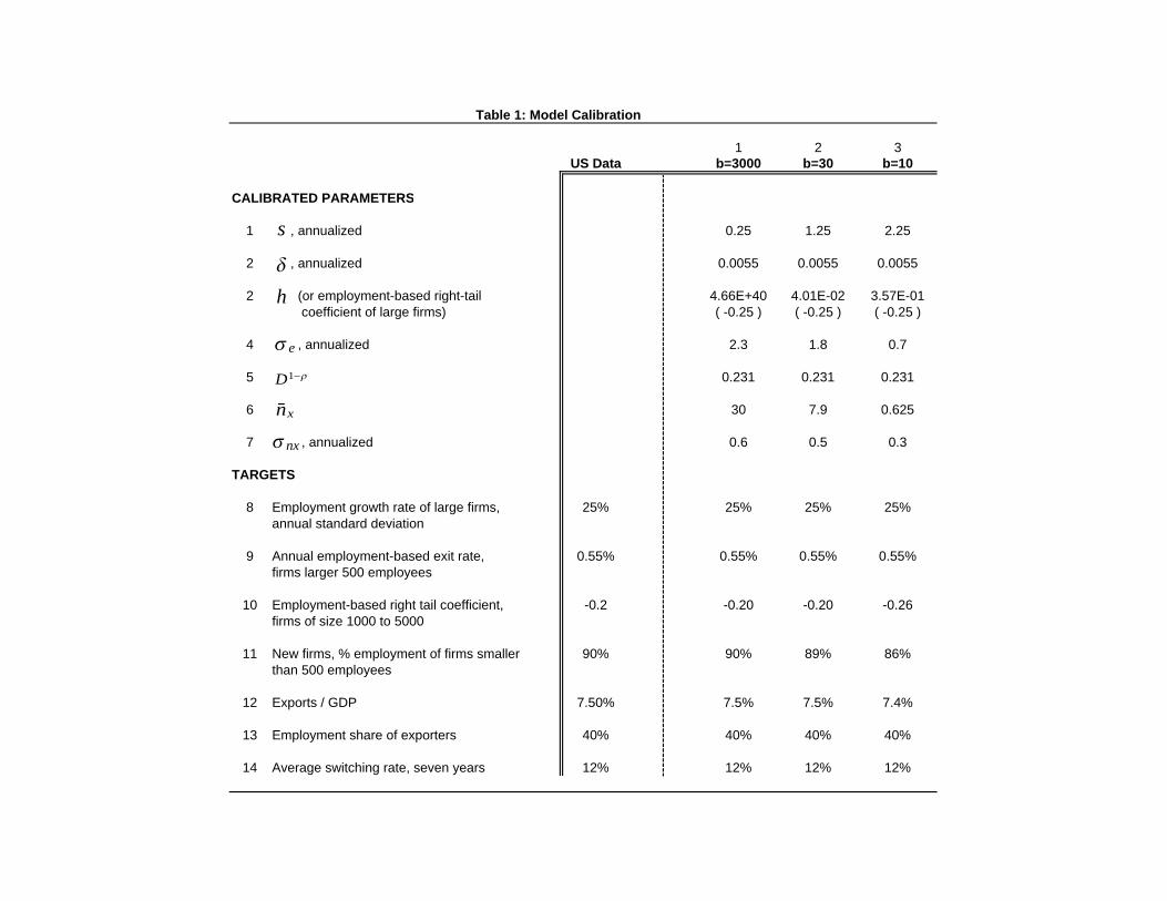
Table 1: Model Calibration

1 2 3US Data b=3000 b=30 b=10

CALIBRATED PARAMETERS

1 , annualized 0.25 1.25 2.25

2 , annualized 0.0055 0.0055 0.0055

2 (or employment-based right-tail 4.66E+40 4.01E-02 3.57E-01 coefficient of large firms) ( -0.25 ) ( -0.25 ) ( -0.25 )

4 , annualized 2.3 1.8 0.7

5 0.231 0.231 0.231

6 30 7.9 0.625

7 , annualized 0.6 0.5 0.3

TARGETS

8 Employment growth rate of large firms, 25% 25% 25% 25%annual standard deviation

9 Annual employment-based exit rate, 0.55% 0.55% 0.55% 0.55%firms larger 500 employees

10 Employment-based right tail coefficient, -0.2 -0.20 -0.20 -0.26firms of size 1000 to 5000

11 New firms, % employment of firms smaller 90% 90% 89% 86%than 500 employees

12 Exports / GDP 7.50% 7.5% 7.5% 7.4%

13 Employment share of exporters 40% 40% 40% 40%

14 Average switching rate, seven years 12% 12% 12% 12%

e

nx

h

D1−

n̄x

s

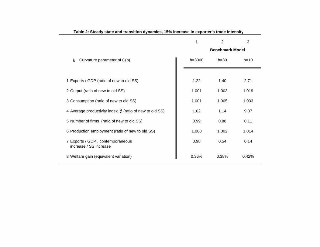
Table 2: Steady state and transition dynamics, 15% increase in exporter's trade intensity

1 2 3

Benchmark Model

Curvature parameter of C(p) b=3000 b=30 b=10

1 Exports / GDP (ratio of new to old SS) 1.22 1.40 2.71

2 Output (ratio of new to old SS) 1.001 1.003 1.019

3 Consumption (ratio of new to old SS) 1.001 1.005 1.033

4 Average productivity index (ratio of new to old SS) 1.02 1.14 9.07

5 Number of firms (ratio of new to old SS) 0.99 0.88 0.11

6 Production employment (ratio of new to old SS) 1.000 1.002 1.014

7 Exports / GDP , contemporaneous 0.98 0.54 0.14increase / SS increase

8 Welfare gain (equivalent variation) 0.36% 0.38% 0.42%

b

z̃

Table 3: Sensitivity Analysis, Steady state and transition dynamics, 15% increase in exporter's trade intensity

1 2 3 4 5 6 7 8 9 10 11 12

Benchmark Higher trade share Lower substitution elasticity Higher variance of entering firms exports / GDP = 0.15

Curvature parameter of C(p) b=3000 b=30 b=10 b=3000 b=30 b=10 b=3000 b=30 b=10 b=3000 b=30 b=10

1 Exports / GDP (ratio of new to old SS) 1.22 1.40 2.71 1.21 1.33 1.90 1.22 1.40 2.71 1.20 1.33 2.44

2 Output (ratio of new to old SS) 1.001 1.003 1.019 1.004 1.007 1.023 1.006 1.024 1.152 1.002 1.003 1.009

3 Consumption (ratio of new to old SS) 1.001 1.005 1.033 1.004 1.010 1.036 1.006 1.028 1.195 1.002 1.004 1.014

4 Average productivity index (ratio of new to old SS) 1.02 1.14 9.07 1.04 1.25 60.67 1.02 1.14 9.07 1.02 1.09 3.72

5 Number of firms (ratio of new to old SS) 0.99 0.88 0.11 0.98 0.82 0.02 0.99 0.89 0.12 0.99 0.92 0.27

6 Production employment (ratio of new to old SS) 1.000 1.002 1.014 1.000 1.002 1.014 1.000 1.005 1.044 1.000 1.001 1.005

7 Exports / GDP , contemporaneous 0.98 0.54 0.14 0.98 0.62 0.25 0.99 0.55 0.14 0.99 0.59 0.14increase / SS increase

8 Welfare gain (equivalent variation) 0.36% 0.38% 0.42% 0.80% 0.83% 0.92% 1.55% 1.81% 2.22% 0.37% 0.38% 0.40%

13 14 15 16 17 18 19 20 21 22 23 24

Higher share of labor in Lower share of labor in Process innovation costs scaled Learning by exporting innovation , innovation , by total employment

Curvature parameter of C(p) b=3000 b=30 b=10 b=3000 b=30 b=10 b=3000 b=30 b=10 b=3000 b=30 b=10

9 Exports / GDP (ratio of new to old SS) 1.22 1.40 2.71 1.22 1.40 2.71 1.22 1.21 1.19 1.22 1.42 2.70

10 Output (ratio of new to old SS) 1.001 1.005 1.032 1.001 1.002 1.011 1.001 1.000 0.999 1.001 1.009 1.076

11 Consumption (ratio of new to old SS) 1.001 1.005 1.033 1.001 1.005 1.032 1.001 1.000 0.999 1.001 1.012 1.120

12 Average productivity index (ratio of new to old SS) 1.02 1.14 9.07 1.02 1.14 9.07 1.02 1.01 0.98 1.02 1.16 8.61

13 Number of firms (ratio of new to old SS) 0.985 0.880 0.114 0.986 0.879 0.112 0.99 0.99 1.02 0.99 0.88 0.13

14 Production employment (ratio of new to old SS) 1.000 1.003 1.024 1.000 1.001 1.007 1.000 1.000 1.000 1.000 1.004 1.049

15 Exports / GDP , contemporaneous 0.98 0.54 0.14 0.98 0.54 0.14 0.99 1.02 1.23 0.99 0.52 0.12increase / SS increase

16 Welfare gain (equivalent variation) 0.36% 0.37% 0.40% 0.35% 0.38% 0.42% 0.35% 0.20% 0.07% 0.36% 0.78% 2.23%

b

b

2

0.95 0.25

z̃

z̃

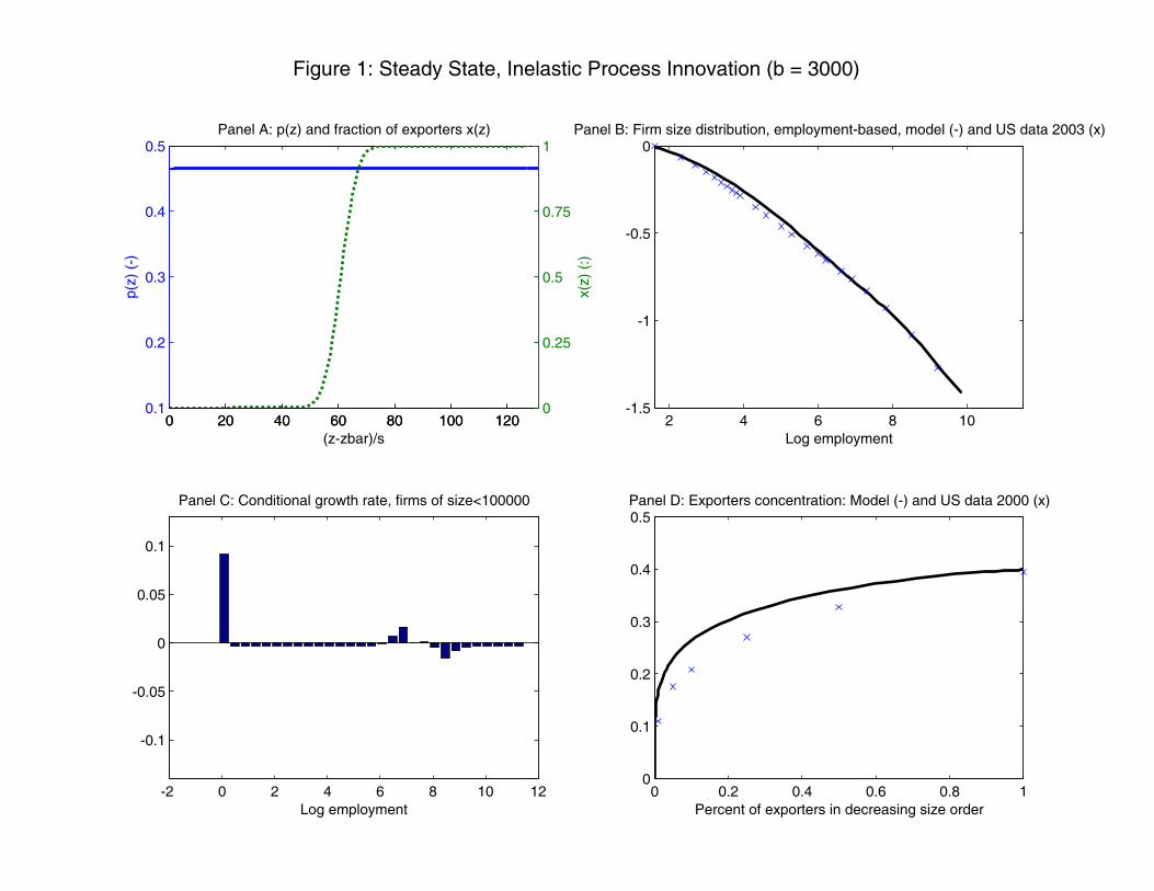
0 20 40 60 80 100 1200.1

0.2

0.3

0.4

0.5p(

z) (

-)Panel A: p(z) and fraction of exporters x(z)

(z-zbar)/s0 20 40 60 80 100 120

0

0.25

0.5

0.75

1

x(z)

(:)

2 4 6 8 10-1.5

-1

-0.5

0Panel B: Firm size distribution, employment-based, model (-) and US data 2003 (x)

Log employment

-2 0 2 4 6 8 10 12

-0.1

-0.05

0

0.05

0.1

Panel C: Conditional growth rate, firms of size<100000

Log employment

Figure 1: Steady State, Inelastic Process Innovation (b = 3000)

0 0.2 0.4 0.6 0.8 10

0.1

0.2

0.3

0.4

0.5Panel D: Exporters concentration: Model (-) and US data 2000 (x)

Percent of exporters in decreasing size order

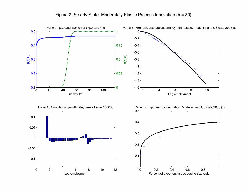
0 20 40 60 80 1000.1

0.2

0.3

0.4

0.5p(

z) (

-)Panel A: p(z) and fraction of exporters x(z)

(z-zbar)/s0 20 40 60 80 100

0

0.25

0.5

0.75

1

x(z)

(:)

2 4 6 8 10-1.6

-1.4

-1.2

-1

-0.8

-0.6

-0.4

-0.2

0Panel B: Firm size distribution, employment-based, model (-) and US data 2003 (x)

Log employment

0 2 4 6 8 10 12

-0.1

-0.05

0

0.05

0.1

Panel C: Conditional growth rate, firms of size<100000

Log employment

Figure 2: Steady State, Moderately Elastic Process Innovation (b = 30)

0 0.2 0.4 0.6 0.8 10

0.1

0.2

0.3

0.4

0.5Panel D: Exporters concentration: Model (-) and US data 2000 (x)

Percent of exporters in decreasing size order

0 20 40 60 80 1000.1

0.2

0.3

0.4

0.5p(

z) (

-)Panel A: p(z) and fraction of exporters x(z)

(z-zbar)/s0 20 40 60 80 100

0

0.25

0.5

0.75

1

x(z)

(:)

2 4 6 8 10-2

-1.5

-1

-0.5

0Panel B: Firm size distribution, employment-based, model (-) and US data 2003 (x)

Log employment

2 4 6 8 10 12

-0.1

-0.05

0

0.05

0.1

Panel C: Conditional growth rate, firms of size<100000

Log employment

Figure 3: Steady State, Highly Elastic Process Innovation (b = 10)

0 0.2 0.4 0.6 0.8 10

0.1

0.2

0.3

0.4

0.5Panel D: Exporters concentration: Model (-) and US data 2000 (x)

Percent of exporters in decreasing size order

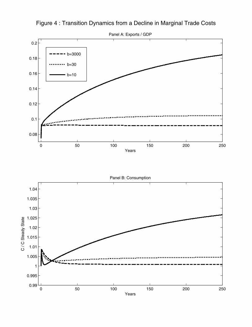
0 50 100 150 200 250

0.08

0.1

0.12

0.14

0.16

0.18

0.2

Years

Panel A: Exports / GDP

Figure 4 : Transition Dynamics from a Decline in Marginal Trade Costs

0 50 100 150 200 2500.99

0.995

1

1.005

1.01

1.015

1.02

1.025

1.03

1.035

1.04

Years

C /

C S

tead

y S

tate

Panel B: Consumption

b=3000

b=30

b=10