Aggregate Implications of Innovation Policy

Andrew Atkeson

UCLA

Ariel Burstein

UCLA∗

August 24, 2014

Abstract

We examine the quantitative impact of changes in innovation policies on aggregate

productivity and output in a baseline Klette-Kortum Neo-Schumpeterian growth model.

We present simple analytical results isolating the specific features and/or parame-

ters of the model that play the key roles in shaping its quantitative implications for

the aggregate impact of innovation policies in the short-, medium- and long-term.

We find in our baseline model that permanent changes in innovation policies cannot

spur a significant change in aggregate productivity over the medium term horizon

(i.e. 20 years) in an economy with a moderate initial growth rate of TFP unless the

change in policy leads to a very large change in the innovation rate spurred by a very

large change in investment in innovation relative to GDP. Moreover, we show that the

medium term dynamics implied by the model are not very sensitive to the parame-

ters of the model that determine the model’s long run implications. We find that one

of the key features of the Klette-Kortum model (and many other Neo-Schumpeterian

growth models) that drive these quantitative implications for the medium term is the

assumption that there is no social depreciation of innovation expenditures.

1 Introduction

Firm’s investments in innovation are large relative to GDP and are likely an important fac-tor in accounting for economic growth over time.1 Many OECD countries use taxes and∗This is a substantially revised version of a previous draft with the same title, NBER Working Paper

17493. We thank Ufuk Akcigit, Philippe Aghion, Costas Arkolakis, Arnaud Costinot, Ellen McGrattan,Juan Pablo Nicolini, Pedro Teles, and Aleh Tsyvinski for very useful comments. We thank the NationalScience Foundation (Award Number 0961992) for research support.

1There is a wide range of estimates of the scale of firms’ investments in innovation. In the new NationalIncome and Product Accounts revised in 2013, private sector investments in intellectual property products

1

subsidies to encourage these investments in the hope of stimulating economic growth.2

To what extent can we change the path of macroeconomic growth over the medium andlong term with tax and subsidy policies aimed at encouraging firms to increase their in-vestments in innovation?

We examine this question in the context of a Klette and Kortum (2004) style Neo-Schumpeterian growth model. As described in Aghion et al. (2013), the Klette-Kortummodel is a highly influential model that links micro data on firm dynamics to firms’ in-vestments in innovation and, in the aggregate, to economic growth in a tractable manner.3

One of the distinguishing features of this model is that there is, potentially, a large gap be-tween the social and the private returns to firms’ investments in innovation. As a result,one cannot use standard growth accounting methods for using data on the private returnsto these investments to infer the implications for the path of aggregate productivity andoutput of innovation policy changes that induce a given change in firms’ investments ininnovation.4

We present simple analytical results approximating the impulse responses of the log-arithm of aggregate productivity and GDP with respect to a policy-induced (i.e.. inno-vation subsidies) change in the logarithm of firms’ spending on innovation relative toGDP. In deriving these results we isolate the specific features and/or parameters of themodel that play the key roles in shaping its quantitative implications for the links be-tween changes in innovation policy and the resulting changes in innovation spending,the innovation rate, and the growth of aggregate productivity and GDP at short, medium,and long horizons. We also use these analytical impulse response functions to highlightthe features of the model that drive its implications for the socially optimal innovationintensity of the economy. We confirm the utility of these analytical approximations by

were 3.8% of GDP in 2012. Of that amount, Private Research and Development was 1.7% of GDP. The re-mainder of that expenditure was largely on intellectual property that can be sold such as films and otherartistic originals. Corrado et al. (2005) and Corrado et al. (2009) propose a broader measure of firms’ invest-ments in innovation, which includes non-scientific R&D, brand equity, firm specific resources, and businessinvestment in computerized information. These broader investments in innovation accounted for roughly13% of non-farm output in the U.S. in 2005.

2See, for example, Chapter 2 of “Economic Policy Reform: Going for Growth”, OECD, 2009.3Several authors (see, for example, Akcigit and Kerr 2010 and Lentz and Mortensen 2008) have shown

that extended versions of the Klette-Kortum model provide a good fit to many features of micro data onfirms.

4There is a very large literature that seeks to use standard methods from growth accounting to capitalizefirms’ investments in innovation and to use the dynamics of that intangible capital aggregate to accountfor the dynamics of aggregate productivity and output. See, for example, Griliches, ed (1987), Kendrick(1994), Griliches (1998), and Corrado and Hulten (2013). Relatedly, McGrattan and Prescott (2012) use anoverlapping generations model augmented to include firms’ investments in intangible capital to ask howchanges in various tax and transfer policies will impact the accumulation of intangible capital and aggregateproductivity and GDP.

2

comparing them to the numerical solution to the equilibrium transition path following achange in innovation policies in a fully calibrated version of the model.

We find in this baseline model that permanent changes in innovation subsidies cannotspur a significant change in aggregate productivity over the medium term horizon (i.e.20 years) in an economy with a moderate initial growth rate of TFP unless the change inpolicy leads to a very large change in the innovation rate spurred by a very large change infirms’ investment in innovation relative to GDP.5 This finding is not sensitive to changesin parameters that determine the long-run implications of the model and the potentialwelfare gains that might be achieved from a sustained increase in innovation subsidies.Thus, in this model, if there are large welfare gains to an infinitely-lived consumer froma permanent increase in innovation subsidies, they are achieved only because of changesin the path of consumption that occur in the long run.

We show analytically that one of the key features of the Klette-Kortum model (andnearly all Neo-Schumpeterian growth models) that drive its quantitative implications forthe short and medium term is the implicit assumption that there is no social depreciationof innovation expenditures. Specifically, in this model, there is private depreciation of pastinvestments in innovation in terms of their impact on firms’ profits — firms gain andlose products and profits as they expend resources to innovate upon the products pro-duced by others. In contrast, there is no social depreciation of these investments in termsof their cumulative impact on aggregate productivity — the contribution of past inno-vation expenditures to aggregate production possibilities never dies out over time.6 Weshow that if one makes the alternative assumption that past innovations experience evenmoderate social depreciation, that is that aggregate productivity would shrink in the ab-sence of investments in innovation by firms, then the model can produce significantlylarger medium-term elasticities of aggregate productivity and GDP to permanent policy-induced changes in the innovation intensity of the economy. In the appendix, we showthat in expanding varieties models along the lines of Luttmer (2007) and Atkeson and

5Comin and Gertler (2006) develop a model of medium-term business cycles based on endogenousmovements in aggregate productivity that includes adoption, variable markups, and variable factor uti-lization. They find that with the combination of these factors, their model can account for significantmedium-term cyclical productivity dynamics. We see our results as highlighting the endogenous dynamicsof aggregate productivity that arise solely from policy-induced variation in the innovation intensity of theeconomy. McGrattan and Prescott (2012) emphasize how measurement conventions for GDP impact themeasurement of aggregate productivity in the face of time variation in the scale of firms’ investments inintangible capital. We discuss the role of different NIPA convention methods for shaping the responses ofmeasured productivity and output.

6Corrado and Hulten (2013), Li (2012) and Aizcorbe et al. (2009) discuss comprehensive estimates of thedepreciation rates of innovation expenditures without distinguishing between measures of the private andsocial depreciation of these expenditures.

3

Burstein (2010) there is social depreciation of innovation expenditures due to the exit ofincumbent firms, but otherwise these models imply very similar expressions for the dy-namics of aggregate productivity as in our baseline Klette-Kortum model. We show thatsince these models have social depreciation of innovation built-in, they can imply largermedium-term elasticities of aggregate productivity with respect to changes in innovationpolicies.7

The Klette-Kortum model provides a rich and yet tractable model of the birth, growth,and death of firms in which these firm dynamics are driven by incumbent and entrantfirms’ investments in innovation. One of the principal innovations of the Klette-Kortummodel relative to the standard Quality Ladders model introduced by Aghion and Howitt(1992) and Grossman and Helpman (1991) is that it considers investments in innovationby both incumbent and entering firms. We show that, given the same change in inno-vation subsidies, the two models imply the same change in innovation intensity andaggregate productivity in the long run, up to a first-order approximation. Moreover,if we consider innovation policy changes in the Klette-Kortum model that produce thesame transition path for the innovation intensity of the economy as the innovation policychanges considered in a Quality Ladders version of the model,8 then the Quality Laddersversion of the model will imply a larger change in aggregate productivity up to any fi-nite horizon along the transition path, up to a first-order approximation. We show thatthis result follows from the assumption in the Klette-Kortum model that incumbent firmshave a smaller average cost of innovation than entering firms.

To focus attention on the aggregate implications of innovation policies that changethe aggregate innovation intensity of the economy, we maintain a baseline set of assump-tions which imply that, while the aggregate level of innovation expenditures may be sub-optimal, there is no misallocation of innovation expenditures across firms in the modeleconomy at the start of the transition following a change in innovation policies. Thus weabstract from the role innovation policies might play in improving the allocation of inno-vation expenditures across firms and thus raising the aggregate innovation rate withoutincreasing aggregate innovation expenditures. There is a growing literature examining

7As we discuss below, the aggregate dynamics implied by our baseline version of the Klette-Kortummodel can also be derived in the simpler model studied in Jones (2002). Since the model of Jones (2002)has no social depreciation of innovations, it also implies modest medium-term elasticities of aggregateproductivity to changes in the innovation intensity of the economy. Consistent with his results, for longertime horizons under certain parameter configurations, a sustained increase in the innovation intensity ofthe economy can have a sustained impact on the growth of aggregate productivity.

8Considering given changes in the innovation intensity of the economy is reminiscent to Arkolakis et al.(2012), who take changes in trade shares as given when comparing the aggregate implications of alternativetrade models.

4

this possibility, see for example Acemoglu et al. (2013), Buera and Fattal-Jaef (2014), andPeters (2013). We see our results as providing a useful analytical benchmark to whichnumerical results from richer models can be compared.

The paper is organized as follows. Section 2 describes the model. Section 3 character-izes a balanced growth path. Section 4 presents analytic results on the impact of changesin innovation policy on aggregate outcomes at different horizons. Section 5 discusses thequantitative implications of our analytic results, and Section 6 compares these results tothe full numerical solution of our calibrated model. Section 7 concludes. The appendixprovides some proofs and other details including the calibration of the model.

2 Model

In this section we describe the physical environment, innovation policies, and the equi-librium.

Physical environment

Time is discrete and labeled t = 0, 1, 2,... There are two final goods, the first of which wecall the consumption good and the second which we call the research good. The representa-tive household has preferences over consumption Ct given by ∑∞

t=0 βtLt log(Ct/Lt), withβ ≤ 1, where Lt denotes the population that is constant and normalized to 1, (Lt = 1).9

Labor can be allocated to current production of the consumption good, Lpt, and to re-search, Lrt. The resource constraint requires that labor used in these two activities mustsum to the fixed total population that we normalize to 1, that is, Lpt + Lrt = Lt = 1.

Production of the consumption good: The consumption good is produced as a constantelasticity of substitution (CES) aggregate of the output of a continuum of measure one ofdifferentiated intermediate products. Each intermediate good is characterized by an in-dex z that denotes the frontier technology for producing that product. These intermediategoods are then combined to produce the consumption good according to

Yt = Apt

(ˆz

yt(z)(ρ−1)/ρdJt(z))ρ/(ρ−1)

, (1)

where Jt(z) denotes the distribution of z across intermediate goods at date t (so´

z dJt(z) =1), Apt denotes a stationary aggregate productivity shock with mean 1 and ρ ≥ 1.

9It is straightforward to extend our analysis to include population growth.

5

Output of the consumption good, Yt, is used for two purposes. First, as consumptionby the representative household, Ct. Second, as investment in physical (tangible) capital,Kt+1 − (1− dk)Kt, where Kt denotes the aggregate physical capital stock and dk denotesthe depreciation rate of physical capital. The resource constraint of the final consumptiongood is

Ct + Kt+1 − (1− dk)Kt = Yt. (2)

Under the national income and product accounting (NIPA) convention that expenditureson innovation are expensed, the quantity in the model corresponding to Gross DomesticProduct (GDP) as measured in the data under historical measurement procedures is equalto Yt.10

Production of an intermediate good with index z is carried out with physical capital,k, and labor, l, according to

yt(z) = exp(zt)kt (z)α lt(z)1−α, (3)

where 0 < α < 1. For each intermediate good, the frontier technology z is owned by anincumbent firm, with exclusive rights to use that technology in production. At the sametime, other firms can produce this product with the technology indexed by z − ∆l. Theparameter ∆l may be be interpreted as a parameter of antitrust (or competition) policy forthe frontier technology z, as discussed in Acemoglu (2009) (see section 13.1.6).

Each incumbent firm is characterized by the number n of intermediate goods that itproduces. Hence, the state variable that characterizes an incumbent firm is a vector ofproductivities z of length n. Let Gt (n) denote the measure of incumbent firms with nproducts at time t. The requirement that each product be owned by some firm implies

∑∞n=1 nGt(n) = 1 for all periods t.

It is straightforward to show that in an equilibrium with equal markups across prod-ucts, aggregate output of the final consumption good, Yt, is given by

Yt = AptZt (Kt)α (Lpt

)1−α , (4)

where Lpt =´

z lt(z)dJt(z), Kt =´

z kt(z)dJt(z), and Zt =[´

z exp(z)ρ−1dJt(z)] 1

ρ−1 . Notethat Zt here corresponds to aggregate productivity in the production of the final consump-

10The treatment of expenditures on innovation in the NIPA in the United States is being revised as ofthe second half of 2013 to include a portion of those expenditures on innovation in measured GDP. If allintangible investments in the model were measured as part of GDP, then measured GDP would be givenby GDPt = Ct + Kt+1 − (1− dk)Kt + PrtYrt, where PrtYrt denotes intangible investment expenditure, asdefined below. We report results on GDP under both measurement procedures.

6

tion good.In general, this model-based measure of aggregate productivity, Zt, does not corre-

spond to measured TFP, which is given by TFPt = GDPt/(

Kαt L1−α

t

), where 1− α denotes

the share of labor compensation in measured GDP. This adjustment is required becauseof the expensing of expenditures on innovation (under historical standards for measur-ing GDP) and because of possible variation over time in the allocation of labor betweenproduction and research. The growth rate of this model-based measure of aggregate pro-ductivity, however, is equal to the growth rate of measured TFP on a balanced growthpath.

Innovation by intermediate goods producing firms: Innovation is conducted by in-cumbent and entering firms. Incumbent firms and entering firms invest innovative effortto improve upon the technology frontier of a product. A firm that succeeds in innovatingon a product raises the frontier from z to z + ∆ and becomes the sole incumbent producerof the product.

The distribution of frontier technologies Jt (z) evolves as follows. Given an initialdistribution Jt (z), an independently drawn fraction of products δt receive increments totheir frontier technologies of size ∆ ≥ ∆l. Hence aggregate productivity grows at the rategzt, where11

exp (gzt) =Zt+1

Zt=[δt exp (∆)ρ−1 + 1− δt

] 1ρ−1 . (5)

We show below that, for the set of policies we consider, it is optimal for every incum-bent firm to engage in the same innovative effort per product it owns, independent ofthe level of z associated with those products. We impose this result here to simplify thenotation. Let each firm with n products engage in a total of nqt units of innovative effortto obtain new products, and let each entering firm engage in one unit of innovative effortto obtain new products. Let Mt be the measure of entrants. Total innovative effort is thengiven by

qt ∑n=1

nGt(n) + Mt = qt + Mt.

11One can show that this model does not have a stationary distribution of firm sizes in a balanced growthpath unless ρ = 1. This is because, without this assumption, there is not a stationary distribution of ex-penditure across products. To ensure a stationary distribution of firm sizes, one can modify the model asfollows, without changing its aggregate implications. Assume that at the end of every period t, after pro-duction and innovation occur, a measure ξ of those products that did not receive an innovation have theirfrontier technology z reset to a new level z′ = log Zt. This reset frontier technology is still owned by thesame incumbent firm. At the same time as this reseting occurs, the technology freely available to otherfirms who may choose to produce this good is reset to log Zt − ∆l . The transition law for Zt is not affectedby the reset probability ξ.

7

Given innovative effort by incumbent and entrant firms, qt and Mt, firms are matchedat random to successful innovations through a matching function. The total measure ofproducts innovated on is given by the matching function

δt = m(1, qt + Mt), (6)

where the first argument of m (·, ·) denotes the measure of products available to be in-novated upon and the second argument denotes the total innovative effort. The functionm (·, ·) is constant returns to scale and increasing in each argument. In what follows weassume that this function takes the form m (1, x) = σ0xσ, with σ ≤ 1 The case of σ = 1 cor-responds to the case in which the rate at which innovations arrive for an innovating firmis independent of the innovative activity of other firms. The case of σ < 1 corresponds tocongestion frictions in innovative activity.

Innovations are divided up at random among incumbent and entrant firms in pro-portion to their innovative effort. An entrant firm that engages in one unit of innovativeeffort obtains a product with probability 1

qt+Mtδt. A firm of size n that engages in nqt

units of innovative effort obtains new products according to a Poisson distribution withparameter n qt

qt+Mtδt.

The research good: We now describe the resource cost of innovative effort. As in Kletteand Kortum (2004), a firm with n products has the option of investing c (qn, n) units of theresearch good to engage in qn units of innovative effort. We assume that c (., .) is constantreturns to scale, so we can rewrite this total investment as nc (q), where c (.) is increasingand convex. In this sense, n indexes an incumbent firm’s innovative capacity as well asits number of products. If the firm chooses not to use this technology, then it invests zerounits of the research good. Entering firms must invest f units of the research good toengage in one unit of innovative effort. Summing investment across firms and using thefact that ∑n=1 nGt(n) = 1 gives the resource constraint for the research good,

c (qt) + f Mt = Yrt. (7)

Production of the research good is carried out using research labor Lrt according to

Yrt = Zγ−1t ArtLrt , (8)

where γ ≤ 1. The variable Art represents the stock of basic scientific knowledge that isassumed to evolve exogenously, growing at a steady rate of gAr so Art+1 = exp(gAr)Art.

8

Increases in this stock of scientific knowledge improve the productivity of resources de-voted to innovative activity. We interpret Art as a worldwide stock of scientific knowl-edge that is freely available for firms to use in innovative activities. The determination ofthis stock of scientific knowledge is outside the scope of our analysis.12 In the Appendixwe consider an extension in which research production uses both labor and consumptiongood, as in the lab-equipment model of Rivera-Batiz and Romer (1991).

We interpret the parameter γ ≤ 1 as indexing the extent of intertemporal knowledgespillovers, that is the extent to which further innovations become more difficult as theaggregate productivity Zt grows relative to the stock of scientific knowledge Art. As γ

approaches 1, the resource cost of innovating on the frontier technology becomes inde-pendent of Zt (hence, there are full spillovers). The impact of advances in Zt on the costof further innovations is external to any particular firm and hence we call it a spillover.Standard specifications of quality ladders models with fully endogenous growth (includ-ing Klette and Kortum 2004) correspond to the case with full spillovers and gAr = 0.

Policies and Equilibrium

We now describe the decentralization of this economy and define equilibrium with a col-lection of policies. In this decentralization, we assume that the representative householdowns the incumbent firms and the physical capital stock, facing a sequence of budgetconstraints given by

Ct + Kt+1 = [Rkt + (1− dk)]Kt + WtLt + Dt − Et,

in each period t, where Wt, Rkt, Dt, and Et denote the economy-wide wage, rental rate ofphysical capital, aggregate dividends paid by firms, and aggregate fiscal expenditures onpolicies (which are financed by lump-sum taxes collected from the representative house-hold), respectively.

Competitive firms producing the final consumption good choose inputs and output tomaximize profits each period subject to (4). By standard arguments, in equilibrium, prices

must satisfy (1 + τs) AptPt =[´

z pt(z)1−ρdJt(z)] 1

1−ρ , where pt (z) is the price set for goodswith productivity index z, Pt is the price of the final good, and τs is a per-unit subsidy

12It is common in the theoretical literature to assume that all productivity growth is driven entirely byfirms’ expenditures on R&D (Griliches 1979, p. 93). As noted in Corrado et al. (2011), this view ignores theproductivity-enhancing effects of public infrastructure, the climate for business formation, and the fact thatprivate R&D is not all there is to innovation. We capture all of these other productivity enhancing effectswith Ar. Relatedly, Akcigit et al. (2013) considers a growth model that distinguishes between basic andapplied research and introduces a public research sector.

9

on production of the consumption good. This production subsidy can be set to undo thedistortions from the intermediate good’s markup. We normalize Pt to 1.

Production of the research good is undertaken by competitive firms that take the in-tertemporal knowledge spillover from innovation as given. Cost minimization in theproduction of the research good implies that the price of the research good, Prt, is equalto

Prt =Z1−γ

tArt

Wt . (9)

Prt is the deflator needed to translate changes in innovation expenditure, PrtYrt, intochanges in innovation output, Yrt. We define the innovation intensity of the economy, srt,as the ratio of innovation expenditure to the sum of expenditure on consumption andphysical capital investment (i.e. the old measure of GDP), that is srt = PrtYrt/GDPt.

Intermediate goods producing firms are offered two types of innovation subsidies.First, incumbent firms receive a subsidy to innovation expenditure, which we denote byτg. Second, entering firms receive a subsidy to innovation expenditure, which we denoteby τe. We refer to policies in which τg = τe as uniform innovation subsidies.

The variable profits that an incumbent firm earns in period t from production of aproduct with productivity index z are given by [pt(z)yt(z) −Wtlt(z)−Rktkt (z)]. The in-cumbent firm that owns this product chooses price and quantity, pt (z) and yt (z), to max-imize these variable profits subject to the demand for its product and the productionfunction (1). We assume that the gross markup µ charged by the incumbent producer ofeach product is the minimum of the monopoly markup, ρ/ (ρ− 1), and the technologygap between the leader and any potential second most productive producer of the good,exp (∆l). That is µ = min

{ρ

ρ−1 , exp (∆l)}

. Variable profits from production can then be

written as Πt exp(z)ρ−1, with the constant in variable profits Πt defined by

Πt = κ0 (1 + τs)ρ Aρ−1

pt

(Rα

ktW1−αt

)1−ρYt, (10)

with κ0 = µ−ρ(µ− 1)[αα (1− α)1−α

]ρ−1. It is straightforward to show that revenues and

employment engaged in production also scale with productivity index z in direct pro-portion to exp(z)ρ−1. Hence, the equilibrium size of a firm with n products with frontiertechnologies z1, ..., zn is directly proportional to exp(z1)

ρ−1 + ... + exp(zn)ρ−1.Incumbent firms that use their innovation technology, choose their innovative effort

to maximize the value of the firm. For owners of a firm, there are two components to thevalue of gaining a product through innovation. One comes from the expected discountedstream of profits it earns from selling the product at a markup over marginal cost for as

10

long as that firm remains the incumbent producer of that product, and the other comesfrom the contribution that its ownership of the product makes to the firm’s innovativecapacity.

The expected discounted stream of profits associated with selling a product with pro-ductivity index z is given by the solution to the following Bellman equation which takesinto account the probability that the firm loses its ownership of this product to anotherinnovating firm

Vt(z) = Πt exp(z)ρ−1 +(1− δt)

1 + rtVt+1 (z) ,

where rt denotes the interest rate denominated in the final consumption good, which withlog preferences is given by 1 + rt = β−1Ct+1/Ct. Integrating this expression across z andusing the definition of the aggregate Zt, we have

ˆz

Vt (z) dJt(z) = VtZρ−1t = ΠtZ

ρ−1t +

(1− δt)

1 + rtVt+1Zρ−1

t , (11)

where Vt = Vt (0).The second component of the value to a firm of owning a product is given by the

contribution of that product to the firm’s innovation capacity. We denote by Ut (n) thevalue of innovative capacity for an incumbent firm with n products. Specifically, Ut (n)corresponds to the expected present value of dividends the incumbent firm expects toearn on products it gains through innovation minus the cost of that innovation. Giventhat c (qn, n) is constant returns to scale, one can show that this value function can bewritten as Utn, where Ut is determined by the Bellman equation

Ut = maxq−(1− τg

)c(q)Prt +

11 + rt

qqt + Mt

δtVt+1Zρ−1t exp (∆)ρ−1 (12)

+1

1 + rt

(q

qt + Mtδt + 1− δt

)Ut+1.

The first term on the right side indicates the investment required of an incumbent firmto engage in q units of innovative effort per product. The second term indicates the dis-counted present value of variable profits the firm expects to gain from the innovationsthat result from this innovative effort. The third term denotes the expected value of thefirm’s innovative capacity from next period on, taking into account both the gain in prod-ucts it expects to obtain from its innovative effort (i.e., a firm with n products expectsto gain q

q+M δn products) and the loss of products it expects as a result of innovative ef-fort from other firms (i.e., a firm with n products expects to lose δn products). Each firm

11

takes as given the innovative effort of other firms, as given by qt, Mt, and δt. Note thatin equilibrium, if the incumbents’ innovation technology is used, we must have Ut ≥ 0.Otherwise, incumbents would choose not to use their innovation technology at all.

The total value of an incumbent firm with n products with frontier technologies z1, ..., zn

is the sum of the values over its current products, ∑ni=1 Vtexp (zi)

ρ−1 plus the value of itsinnovative capacity, Utn. The free entry condition for new firms is given by

(1− τe) Prt f ≥(

11 + rt

δt

qt + Mt

)(Vt+1Zρ−1

t exp (∆)ρ−1 + Ut+1

), (13)

with this condition holding with equality if the measure of entering firms, Mt, is greaterthan zero.

The government’s aggregate fiscal expenditures on policies in equilibrium are givenby

Et = τgc (qt) Prt + τe f MtPrt + τsYt. (14)

Definition of Equilibrium: An equilibrium in this economy is a collection of sequencesof aggregate prices {rt, Prt, Rkt ,Wt}, prices for intermediate goods {pt(z)}, sequences ofaggregate quantities {Yt,Ct,Lpt,Lrt}, quantities of the intermediate goods and allocationsof physical capital and labor {yt(z), kt (z) , lt (z)} sequences of {Πt}, and sequences offirm value functions and innovation decisions {Vt, Ut, qt, Mt} together with distributionsof firms and aggregate productivities {Jt(z), Zt} such that, given a set of policies

{τe, τg, τs

},

initial stocks{

Ar0, Ap0, L0, K0}

, and an initial distribution of productivities J0(z), house-holds maximize their utility subject to their budget constraint, intermediate good firmsmaximize profits, all of the feasibility constraints are satisfied, and the distribution offirms evolves as described above.

Key assumptions for our aggregate analysis

In specifying our model, we have made four key assumptions that make our modeltractable for analysis of the aggregate implications of changes in innovation policies. Withthese assumptions, we show that the model allows for aggregation in the sense that, atthe margin, changes in the growth rate of aggregate productivity are a function only ofchanges in firms’ aggregate expenditure on innovation and not on the distribution of in-novation expenditure across the heterogeneous firms in the economy.

12

(i) Uniform markups: We have already discussed that the assumption of uniform markupsacross products allows us to construct the index Zt of aggregate productivity whose lawof motion is determined by the aggregate innovation rate δt as shown in expression (5).In the appendix we show that it is sufficient for our simple aggregation to assume thatthe distribution of markups is constant over time and uncorrelated with product produc-tivity z. In this way, the model can be extended to include cross-section variation in laborrevenue productivity.

(ii) And uniform innovation step size: In our specification of the environment andour definition of equilibrium, we assumed that all incumbent firms engage in the sameamount of innovative effort per product that they own. This result follows from ourassumptions of uniform markups across products and uniform innovation step size ∆across products. To see this, consider the first-order condition from equation (12) for op-timal innovative effort per product by incumbent firms, qt, which is given by

(1− τg

)Prtc′(qt) =

(1

1 + rt

δt

qt + Mt

)(Vt+1Zρ−1

t exp (∆)ρ−1 + Ut+1

). (15)

Since none of the terms depend on the incumbent firm’s number of products n or theproductivities with which the firm can produce those products, we have that qt = qt forall products and firms. In the appendix we show that the property that all incumbentfirms choose the same qt extends in an alternative specification of our model in whicheach product that is innovated on draws a random markup and innovation step size thatis independent of the identity of the innovator. In this alternative specification of themodel, there is persistent variation in labor revenue productivity and in research intensity(e.g. innovation expenditures relative to revenues) that is not correlated with firm growth(as emphasized in Klette and Kortum 2004).

(iii) And free entry: If the equilibrium has entering firms, then the zero-profit conditionfor entry (13) and equation (15) imply that if Mt > 0 all incumbent firms innovate at thesame rate qt = qt per product that they own determined from

(1− τg

)c′(qt) = (1− τe) f . (16)

This result implies that in any equilibrium with positive entry and uniform innovationsubsidies, c′(q) = f , i.e. the marginal resource cost of innovative effort is equated acrossfirms. We show that this implies that the equilibrium distribution of innovative effort

13

across firms in this case is conditionally efficient in the sense that a social planner would notwant to reallocate innovative effort across firms (both entrants and incumbents), holdingfixed the level of research output.

(iv) And constant factor shares: Finally, to compute how production of the researchgood Yr changes with changes in expenditure on innovation relative to GDP sr , we makeuse of the following results about the division of GDP into payments to various factors ofproduction and the relationship of those factor shares to the innovation intensity of theeconomy and the allocation of labor.

With CES aggregators and Cobb-Douglas production functions, aggregate revenuesof intermediate goods firms, (1 + τs)Yt, are split into three components. A share µ−1

µ

accrues to variable profits from production, ΠtZρ−1t = µ−1

µ (1 + τs)Yt, a share α/µ ispaid to physical capital, RktKt =

αµ (1 + τs)Yt, and a share (1− α) /µ is paid as wages to

production labor, WtLpt =(1−α)

µ (1 + τs)Yt.With perfect competition in the research sector, WtLrt = PrtYrt. Using the factor shares

above, the allocation of labor between production and research is related to expenditureson the research good by13

Lpt

Lrt=

(1− α) (1 + τs)

µ

1srt

. (17)

In the appendix we show that a similar expression holds in a version of the model withrandom markups across products as discussed above.

3 Balanced growth path

We now characterize the main features of a balanced growth path (BGP) of the equi-librium of our model. We provide additional details of this characterization in the ap-pendix. Our model has two types of BGPs, one with semi-endogenous growth and onewith endogenous growth, depending on the parameter γ. If γ < 1, then our model is asemi-endogenous growth model with the growth rate along the BGP determined by theexogenous growth rate of scientific knowledge gAr and other parameter values indepen-dently of innovation policies, as in Kortum (1997) and Jones (2002). In this case, it is not

13Here we are assuming that there is one wage for labor in both production and research. In the Appendixwe present an extension in which labor is imperfectly substitutable between production and research as inJaimovich and Rebelo (2012). The assumption of imperfect substitutability reduces the elasticity of the allo-cation of labor between production and research with respect to a policy-induced change in the innovationintensity of the economy, resulting in even smaller responses of aggregate productivity and GDP to a givenchange in the innovation intensity of the economy relative to those in our baseline model.

14

possible to have fully endogenous growth because such growth would require growth ininnovation expenditure in excess of the growth rate of GDP. Ongoing balanced growthcan occur only to the extent that exogenous scientific progress reduces the cost of furtherinnovation as aggregate productivity Z grows. In the knife edged case that γ = 1 andgAr = 0, our model is an endogenous growth model with the growth rate along the BGPdetermined by firms’ investments in innovative activity, as in Grossman and Helpman(1991) and Klette and Kortum (2004).14

The transition paths of the response of aggregates to policy changes are continuous asγ approaches one. Hence, our analysis of the model’s quantitative implications for theresponse of aggregates in the medium term (20 years) in the semi-endogenous growthcase nests the endogenous growth case.

In the semi-endogenous growth case, γ < 1, the growth rates of aggregates and the in-terest rate are independent of policies and determined from equations (2), (4), (7), and (8).In particular, the growth rate of aggregate productivity gz is given by gz = gAr/(1− γ).The growth rate of output of the consumption good (and hence consumption, physicalcapital, and the wage) is given by gy = gz/ (1− α), and the rental rate of capital is con-stant and given by Rk = β−1 exp

(gy)− 1 + dk. The rate at which innovations occur, δ,

is pinned down from (5). The matching function (6) pins down total innovative effort,q + M. Innovation by incumbent firms q is constant and, with positive firm entry, is de-termined as the solution to (16). Equilibrium entry M is then calculated as a residual.Note that, in the BGP, policies affect the division of innovative effort between incumbentsand entering firms, but not the total innovative effort q + M nor the rate of innovation δ.

We focus on parameter values such that on the BGP, new firms enter (so M > 0) andincumbents choose to use their innovation technology. To have firm entry in a BGP withinnovation by incumbent firms, it must be that the solution for M described above ispositive. Incumbent firms find it optimal to use their innovation technology in a BGPwith firm entry if and only if at the q that solves equation (16), the post-subsidy averagecost of innovation for incumbent firms,

(1− τg

)c (q) /q, is less than or equal to the post-

subsidy average cost of innovation for entrants, (1− τe) f (we prove this statement in theappendix). This condition is equivalent to the statement c(q) ≤ c′(q)q at that q. This holdsif c(q) is convex and c(0) = 0.

In applying this model to data, we will calibrate the parameters to match a given BGPper capita growth rate of output, gy. Given a choice of gy and physical capital share ofα, the growth rate of aggregate productivity in the BGP is gz = gy (1− α) independent

14If γ > 1, then our model does not have a BGP, as in this case, a constant innovation intensity of theeconomy leads to an acceleration of the innovation rate as aggregate productivity Z grows.

15

of γ. This implies that the aggregate innovation rate δ on the BGP is also independentof γ. For a given choice of γ, the growth rate of scientific knowledge consistent withthese productivity growth rates is given by gAr = (1− γ) gz. We assume that gAr isunmeasured and hence do not make assumptions about this growth rate directly. Instead,we alter this parameter as we vary γ.

4 Aggregate implications of changes in the innovation in-

tensity of the economy: Analytic results

In this section, we derive analytic results regarding the impact of policy-driven changes inthe innovation intensity of the economy on aggregate outcomes at different time horizons.These analytical results demonstrate what features of our baseline Klette-Kortum modelare key in determining its implications for the aggregate impact of innovation policies. Inthe next section, we discuss the quantitative implications of our analytical results.

In framing the question of how policy-induced changes in the innovation intensity ofthe economy impact aggregate outcomes at different time horizons, we consider the fol-lowing thought experiment. Consider an economy that is initially on a BGP with uniforminnovation subsidies, τe = τg. As a baseline experiment (which we relax later), consideran unanticipated permanent change in innovation policies to new uniform innovationsubsidies τ′e = τ′g beginning in period t = 0 and continuing on for all t > 0. We keep theproduction subsidy τs constant.

Given our baseline policy experiment, we first derive the elasticity across BGPs of theinnovation intensity of the economy and fiscal expenditures on innovation policies withrespect to this policy experiment. We then derive analytical first-order approximationsto the change in the transition path and the long run response of aggregate productivityand GDP as a function of this transition path for the innovation intensity of the economy.We then relate the parameters determining the transition dynamics of GDP to those thatshape the optimal innovation intensity of the economy. We next consider non-uniformchanges in innovation policy. Finally, we compare the implications of our model to thoseof a standard quality ladders model in which innovation is only carried out by enteringfirms.

Fiscal impact and innovation intensity across BGPs The following proposition derivesthe elasticity across BGPs of the innovation intensity of the economy and fiscal expendi-tures on innovation policies with respect to a uniform change in innovation policies.

16

Proposition 1. Consider an economy on a BGP with semi-endogenous growth and positive firm-entry. Suppose that innovation policies change permanently from τg = τe to τ′g = τ′e . Then,across the old and new BGP the innovation intensity of the economy changes from sr to s′r, andfiscal expenditures relative to GDP change from E/ ¯GDP to E′/GDP′, with these changes givenby

log s′r − log sr = log(1− τg)− log(1− τ′g)

andE′

GDP′− E

¯GDP= s′r − sr.

The proof of this proposition, which is in the appendix, uses the free-entry condition,which implies that the ratio of aggregate variable profits to the post-subsidy price of theresearch good, ΠZρ−1

(1−τg)Pr, as well as output of the research good, Yr, are both constant across

two BGPs with semi-endogenous growth and uniform innovation subsidies. Togetherwith the fact that aggregate profits are a constant share of GDP, we obtain that sr

(1− τg

)is also constant across BGPs, which implies the first expression. The second expressionfollows from this result and the definition of fiscal expenditures in expression (14).

Proposition 1 implies that in the long-run, our policy experiment will result in a changein the innovation intensity of the economy determined only by the change in the innova-tion subsidy rate independent of the other parameters of the model. At short and mediumhorizons, however, this policy will result in a change in the path of the innovation inten-sity of the economy from {srt}∞

t=0 (which is constant on the initial BGP) to {s′rt}∞t=0 that

we will have to solve for numerically. For the remainder of our analytic results, we takethis path as given.

Dynamics of aggregate productivity and GDP The following proposition characterizesthe transition dynamics of aggregate productivity to a change in the innovation intensityof the economy.

Proposition 2. Consider an economy on a BGP with uniform innovation subsidies and positivefirm-entry. Suppose that at time t = 0, an unanticipated, permanent, and uniform change in inno-vation policies induces a new path for the innovation intensity of the economy given by {s′rt}

∞t=0.

Then the new path for aggregate productivity {Z′t}∞t=1 to a first-order approximation is given by

log Z′t − log Zt =t

∑k=1

Γk(log s′rt−k − log sr

)(18)

17

where Zt = exp(tgz)Z0, with

Γ1 = LpΦσ

ρ− 1exp ((ρ− 1)gz)− 1

exp ((ρ− 1)gz)≤ LpΦσgz, (19)

andΓk+1 =

[1− (1− γ)

Γ1

Lp

]Γk, (20)

where sr denotes the innovation intensity, Lp the share of labor employed in current production,gz the growth rate of aggregate productivity, and

Φ =M/(q + M)

f M/Yr≤ 1 (21)

the ratio of innovative effort by entrants relative to total innovative effort over research expenditureby entrants relative to total research expenditure, where M, q, and Yr denote research effort byentrants and incumbents and research output, all on the initial BGP.

Proof. We prove this result by calculating three key elasticities in our model. The first keyelasticity is the elasticity of research output Yr with respect to a change in the innovationintensity of the economy sr. From equations (8) and (17) we have that, to a first-orderapproximation,

log Y′rt − log Yr = Lp(log s′rt − log sr

)− (1− γ)

(logZ′t − log Zt

). (22)

Hence, this elasticity is given by Lp.The second key elasticity is the elasticity of the innovation rate with respect to a change

in research output. Here from equation (6) we have that, to a first-order approximation,

log δ′t − log δ = σM

q + M(log M′t − log M

)+ σ

qq + M

(log q′t − log q

). (23)

From equation (7) we have that, to a first order approximation

log Y′rt − log Yr =

f MYr

(log M′t − log M

)+

c′(q)qYr

(log q′t − log q

). (24)

From equation (16), we have that with a uniform subsidies log q′t = log q for all t ≥ 0.Combining (23) and (24) we have

log δ′t − log δ = σΦ(

log Y′rt − log Yr

). (25)

18

Hence, this elasticity is given by σΦ.Finally, the third key elasticity is the elasticity of aggregate productivity growth with

respect to the innovation rate. From equation (5) we have that this elasticity is given by

log Z′t+1 − log Z′t ≈ gz +1

ρ− 1exp ((ρ− 1) gz)− 1

exp ((ρ− 1) gz)

(log δ′t − log δ

)(26)

which is equivalent to

log Z′t+1 − log Zt+1 ≈ log Z′t − log Zt +1

ρ− 1exp ((ρ− 1) gz)− 1

exp ((ρ− 1) gz)

(log δ′t − log δ

). (27)

Hence, this elasticity is 1ρ−1

exp((ρ−1)gz)−1exp((ρ−1)gz)

.Plugging in (22) and (25) into (27) gives

log Z′t+1 − log Zt+1 =

[1− (1− γ)

Γ1

Lp

] (log Z′t − log Zt

)(28)

+Γ1(log s′rt − log sr

),

which proves the main result.To show that Φ ≤ 1 in equation (21), recall that in any BGP with innovation by both

incumbent and entering firms, (1− τg)c(q)/q ≤ (1− τe) f . With uniform innovation poli-cies in that BGP, that implies that c(q) ≤ f q. This is sufficient to guarantee that Φ ≤ 1.The case in which incumbents do not use their innovation technology is discussed inProposition 4.

The last step to derive the upper bound on Γ1 in equation (19) is to show that the elas-ticity of aggregate productivity growth with respect to the innovation rate, 1

ρ−1exp((ρ−1)gz)−1

exp((ρ−1)gz),

is bounded above by gz. To do so we use a more general argument (which we apply belowwhen we introduce social depreciation of innovation expenditures and when we discussother models). We write the transition law for aggregate productivity (5) as

Zt+1

Z1= G(δt), (29)

where logG (δ) is concave in δ and log G(δ) = gz. Log-linearizing this equation gives

log Zt+1 − log Zt = log G(δ) +G′(δ)δG(δ)

(log δt − log δ

).

Because G is log-concave, we have that the elasticity of aggregate productivity growth

19

with respect to the innovation rate is bounded above by

G′(δ)δG(δ)

≤ logG(δ)− logG(0) = gz, (30)

where the equality follows from the assumption that G(0) = 1.15 To see how tight thisbound is note that by direct calculation,

G′(δ)δG(δ)

=1

ρ− 1G(δ)ρ−1 − G(0)ρ−1

G(δ)ρ−1 . (31)

Given G(δ) = exp (gz) and G (0) = 1, we have that for any fixed gz > 0 as ρ approaches 1from above this elasticity approaches gz, while as ρ gets large this elasticity limits to zero.

Proposition 2 gives us an analytical expression for the dynamics of aggregate produc-tivity in the transition to a new BGP following an unanticipated, permanent, and uniformchange in innovation policies as a function of the transition path for the innovation inten-sity of the economy that arises in equilibrium as a result of that change in policies. FromProposition 1, we can compute the long-run change in the innovation intensity of theeconomy that arises as a function of a given permanent and uniform change in innovationpolicies. In the next corollary, we derive the long-run change in aggregate productivitythat corresponds to that change in innovation intensity.

Corollary 1. Consider a permanent uniform change in innovation policies. Assume that the econ-omy converges to a new BGP with innovation intensity s′r. Then, the gap in aggregate productivitybetween the old and new BGP converges, to a first-order approximation, to

log Z′t − log Zt =Lp

1− γ

(log s′r − log sr

)(32)

in the semi-endogenous growth case (γ < 1). In the endogenous growth case (γ = 1) the gapin aggregate productivity between the old and new BGP is unbounded. The new growth rate of

15To derive this inequality, we use

G′(·)δG(·)

∣∣∣∣δ=δ

=∂ log G(δ)

∂δ

∣∣∣∣δ=δ

δ ≤(logG(δ)− logG(δ′)

) δ

δ− δ′

for 0 ≤ δ′ < δ, where the inequality follows from concavity of logG(δ). With δ′ = 0, we obtain expression(30).

20

aggregate productivity to a first-order approximation is given by

log Z′t+1 − log Z′t = gz + Γ1(log s′rt − log sr

). (33)

Proof. To derive expression (32) we use equation (22) and the fact that, in response touniform innovation policies, δ, q, M and hence Yr remain constant between BGPs. Notethat Lp

1−γ is equal to ∑∞k=1 Γk in expression (18) if that sum converges. With endogenous

growth, γ = 1, and hence Γk = Γ1 for all k . Equation (33) follows from taking the firstdifference of equation (18).

We next derive the transition path for GDP as a function of the transition paths for ag-gregate productivity, the innovation intensity of the economy, and the equilibrium rentalrate on physical capital.16

Corollary 2. The path of GDP corresponding to the policy experiment in Proposition 2 is given,to a first-order approximation, by

log GDP′t − log ¯GDPt =1

1− α

(log Z′t − log Zt

)− Lr

(log s′rt − log sr

)− α

1− α

(log R′kt − log Rk

)(34)

under the old measurement system in which innovation is expensed, and is given by the above plussr

1+sr(log s′rt − log sr) under a measurement system in which all expenditures on innovation are

included in measured GDP.

Proof. We prove this result by taking the log of GDP, which under the old measurementsystem is equal to the log of Y:

log Y′t − log Yt= log Z′t − log Zt+α(log K′t − log Kt)+(1− α)(

log L′pt − log Lp

)Using Rkt =

αµ (1 + τs)

YtKt

and equation (17) we obtain the expression above. To derive theresult under the new measure of GDP, we must add in expenditures on research PrtYrt,which we can do by multiplying the old measure of GDP by (1 + srt).

Given the result in Corollary 2, it is straightforward to calculate the response of GDPin the long run. Since, with semi-endogenous growth, in the long run the interest rate andrental rate on physical capital return to their levels on the initial BGP (i.e limt→∞ log R′kt−

16The magnitude of the change in the rental rate of physical capital in the transition is related to theequilibrium transition path for the interest rate. From the Euler equation for physical capital, log R′kt −log Rk = r

dk+r log (rt−1/r) for t ≥ 1. Solving for the path of the interest rate requires fully solving for themodel transition, which we do in Section 6.

21

log Rk = 0), the long run response of GDP is a simple function of the long run responsesof aggregate productivity and the innovation intensity of the economy. In particular, fromCorollary 1, we have that with γ < 1, the long run response of GDP is given by

limt→∞

log GDP′t − log ¯GDPt =

[1

1− α

Lp

1− γ− Lr

]limt→∞

(log s′rt − log sr

).

Aggregate dynamics and optimal innovation intensity Expression (34) in Corollary 2is useful for understanding the transition dynamics of measured GDP (corresponding tothe resources available for consumption and physical investment). With a permanent in-crease in the innovation intensity of the economy, GDP falls initially as labor is reallocatedfrom current production to research, and then grows in the transition as the impact of apermanent change in the innovation intensity of the economy on aggregate productivitycumulates over time.

The impact on welfare of a permanent increase in the innovation intensity of the econ-omy clearly depends on the trade-off between the short and long run changes in GDPthat result from this increase in innovation expenditures as captured by the parametersΓk. To gain intuition for this welfare tradeoff, consider a variation in innovation policiesthat raises the innovation intensity of the economy only in period t = 0, so s′r0 > sr and inall other time periods t 6= 0, s′rt = sr. From Corollary 2, if we ignore changes in the rentalrate on physical capital, we have that the log of resources available for consumption andphysical investment (i.e. GDP) falls in period t = 0 by Lr (log s′0 − log sr) and rises inevery period t ≥ 1 by Γt

1−α (log s′0 − log sr). In the appendix, we show that on the optimalBGP allocation, this perturbation of the path of innovation expenditures has no first or-der impact on welfare, which is equivalent to the condition that the socially optimal BGPallocation must satisfy [

∞

∑k=1

βk Γk1− α

− Lr

] (log s′0 − log sr

)= 0

for small perturbations of sr. This condition implies that on the optimal BGP allocation,17

s∗r = (1− α)L∗rL∗p

=β

Γ∗1L∗p

1− β[1− (1− γ)

Γ∗1L∗p

] , (35)

where s∗r , L∗r , and L∗p are the optimal BGP levels of these variables and Γ∗1 is from equation

17One can also obtain this expression using the variational argument proposed by Jones and Williams(1998).

22

(19) evaluated at these optimal quantities. Note from equation (19) that Γ∗1L∗p

is determinedby σ, Φ, ρ and gz. Hence, the optimal innovation intensity of the economy is solely deter-mined by these variables, together with β and γ.

From Proposition 1, we have that if we hold the production subsidy τs constant, theuniform innovation subsidies τ∗g = τ∗e needed to implement a change across BGPs froman initial innovation intensity sr and initial subsidies τg = τe to innovation intensity s∗r isgiven by

log(1− τ∗g ) = log(1− τg) + log sr − log s∗r

and the corresponding fiscal expenditure on innovation subsidies required is E∗/GDP∗−E/ ¯GDP = s∗r − sr. In the appendix we derive the uniform innovation subsidy and pro-duction subsidy to implement the optimal allocation as a function of the parameters ofthe model.

Non-uniform changes in innovation policies So far we have only considered uniformchanges in innovation policies. We now show that if the economy starts on an initial BGPwith uniform innovation policies, then the first-order approximation for the transitionpath of aggregate productivity derived in Proposition 2 does not depend on the particularspecification of changes in policies τe and τg that is used to induce a given path for theinnovation intensity of the economy.

Corollary 3. Consider an economy on an initial BGP as in Proposition 2 that experiences a changein innovation policies at time t = 0 that is unanticipated but not uniform, i.e. with τ′e 6= τ′g. Letthe new path for the innovation intensity of the economy given by {s′rt}

∞t=0. Then the new path for

aggregate productivity and GDP to a first order approximation are given as in Proposition 2 andCorollary 2.

Proof. In deriving the elasticity of the innovation rate with respect to a change in researchoutput in Proposition 2 we used the fact that with uniform changes in innovation policies,log q′t − log q = 0. With non-uniform changes in innovation policies, log q′t − log q 6= 0.Combining (23) and (24) we have that, up to a first order approximation,

log δ′t − log δ = σΦ(

log Y′rt − log Yr

)+ σ

qq + M

(1− c′(q)

f

) (log q′t − log q

).

Starting with uniform innovation policies, τe = τg, equation (16) implies that c′(q) = f , soexpression (25) still holds. The other two key elasticities do not depend on log q′t − log q,so they are also unchanged. The response of GDP is calculated using the same steps as inCorollary 2.

23

Comparing models with and without innovation by incumbent firms So far, we haveconsidered a Klette-Kortum style model that includes innovation by incumbent and en-tering firms. The standard Quality Ladders model introduced by Aghion and Howitt(1992) and Grossman and Helpman (1991) features innovation only by entering firms.Here we compare the aggregate implications of changes in innovation policies in thesetwo types of models.

We can nest the Quality Ladders model in our framework by assuming that c(0) issufficiently high so that c(q) > f q . In this case, incumbent firms will choose not to usetheir innovation technology. The equations characterizing equilibrium in this case haveqt = 0 and c(qt) = 0 in equations (6), (7), and Ut = 0 in equation (13) above. By directcalculation, the parameter Φ defined in Proposition 2 is equal to one in this case.

To compare the aggregate implications of these models, consider a Quality Laddersversion of the model and a Klette-Kortum version of the model that share the same pa-rameter values for γ, σ, α, µ, gAr, and the same production subsidy τs. Let the initial inno-vation subsidies in the Klette-Kortum version of the model be uniform (τg = τe). Let theinitial innovation subsidies in the Quality Ladders version of the model be chosen suchthat the innovation intensity of this economy (and hence the allocation of labor betweenproduction and research) on the initial BGP is the same as for the Klette-Kortum versionof the model on its initial BGP.

We then have the following proposition regarding the impact of uniform changes inpolicies in the long run for these two versions of the model.

Proposition 3. Consider a Klette-Kortum model and a Quality Ladders model that are calibratedequivalently as described above and have semi-endogenous growth (γ < 1). Assume an unan-ticipated, permanent, and uniform change of policies in the two models such that the change inthe log of the subsidy to entering firms, log(1− τe), is the same. Then both models produce thesame change in the innovation intensity of the economy, aggregate productivity, GDP, and fiscalexpenditures on innovation subsidies relative to GDP as a result of this change in policies from theold BGP to the new BGP.

Proof. This result follows from the fact that the long-run change in aggregate productivity,GDP and fiscal expenditures derived above is independent of the value of Φ.

It is more difficult to make comparisons between these two models’ implications forthe transition path from the initial BGP to the new BGP. This is because the equilibriumpath of the innovation intensity in the transition {s′rt}may differ between the two models.We do not have analytical results regarding this transition path. However, we can com-pare the implications of the two models for {Γk} that determine elasticities of aggregate

24

productivity and GDP with respect to the innovation intensity of the economy. We do soin the following Proposition.

Proposition 4. Consider a Klette-Kortum and a Quality Ladders version of the model calibratedequivalently as described above. Then the elasticities

{ΓKK

k}

in the Klette-Kortum version of the

model are related to the elasticities{

ΓQLk

}in the Quality Ladders version of the model defined in

proposition 2 as follows. For any T ≥ 1,

T

∑k=1

ΓKKk ≤

T

∑k=1

ΓQLk .

With semi-endogenous growth, γ < 1, as T → ∞

∞

∑k=1

ΓKKk =

∞

∑k=1

ΓQLk

while with endogenous growth (γ = 1), ΓKKk = ΓKK

1 ≤ ΓQL1 = ΓQL

k for all k ≥ 1.

Proof. For both models, we have,

T

∑k=1

Γk =Lp

1− γ

[1−

(1− (1− γ)

Γ1

Lp

)T]

.

The result follows from the observation that Φ = 1 in the Quality Ladders model andΦ ≤ 1 in the Klette Kortum model, so that ΓKK

1 ≤ ΓQL1 .

What this result implies is that if we consider innovation policy changes in the Klette-Kortum model that produce the same transition path for the innovation intensity of theeconomy {s′rt} as the innovation policy changes considered in the Quality Ladders ver-sion of the model, then the Quality Ladders version of the model will imply a largerchange in aggregate productivity up to any period T along the transition path, to a first-order approximation. In the long-run, as T → ∞, with semi-endogenous growth, the twomodels deliver the same response of aggregate productivity and GDP. Likewise, with en-dogenous growth, for every T, the response of the growth rate will be larger in the QualityLadders version of the model than in the Klette-Kortum version of the model, again to afirst-order approximation.

Note from Corollary 3 that the result in Proposition 4 does not depend on the as-sumption that the policy change in the Klette Kortum version of the model is uniform.Innovation policy changes that are not uniform in that version of the model will impact

25

the innovation decisions of incumbents. To a first-order approximation, holding fixeda transition path for the innovation intensity of the economy, changes in the innovationdecisions of incumbent firms do not impact the aggregate implications of that model.

5 Quantitative implications of analytical results

In this section, we illustrate with a particular numerical example (based on the full cal-ibration of the model discussed in Section 6 and the Appendix) the use of our simpleanalytical results for quantitative analysis of the aggregate implications of changes in in-novation policies in our model. In Section 6, we assess the accuracy of the approximationsthat we make here by numerically computing the equilibrium of the fully specified model.

Consider a calibration of our model in which the time period is set to one year andthe growth rate of aggregate productivity on the initial BGP is gz = .0125, or 1.25%, sothat (for our choice of α) the growth rate of output per worker is 2%, similar to that ex-perienced in the United States over the postwar period. We set ρ = 4 and assume thatthe initial innovation intensity of the economy is sr = .11, similar to the levels estimatedby Corrado et al. (2009) for the United States over the last few years. In the full calibra-tion of the model described in the appendix, this innovation intensity of the economycorresponds to a share of labor employed in current production of Lp = .833 and wecalibrate the innovation cost function for incumbent firms, c(q), such that the parameterΦ = .966 is close to its maximum value of one. We assume that there is no congestionin the mapping from innovation effort to the innovation rate, and hence we have σ equalto its maximum value of one. With these assumptions, the elasticity of aggregate pro-ductivity with respect to changes in the innovation intensity of the economy is given byΓ1 = .01, very close to its upper bound in equation (19).18 Moreover, this value of Γ1 isclose to its largest feasible value equal to gz = .0125. Hence, we regard this numericalexample as useful in illustrating close to a best case scenario for finding large responsesof aggregate productivity to changes in the innovation intensity of the economy and highsensitivity of these responses to the degree of intertemporal knowledge spillovers.

The only other parameter of the model that we need to specify to apply our analyticalresults is the intertemporal knowledge spillover parameter γ which, together with Lp andΓ1 determine the decay rate of the elasticities Γk. We consider three alternative values ofthe intertemporal knowledge spillover parameter γ. The first case we call the high spillovercase. In it we set γ→ 1. The second case we call the medium spillover case, and in it we set

18Recall from equation (19) that as ρ approaches 1, a value that is commonly used in the literature, Γ1approaches the upper bound of LpΦσgz = 0.01. With ρ = 4, we have Γ1 = .00987.

26

γ = 0. The third case we call the low spillover case, and in it we set γ = −2.Consider an unanticipated, uniform, and permanent increase in innovation subsidies

that, in the long run requires an increase in fiscal expenditure on these policies equal to3 percent of GDP. Note that this is a large change in fiscal expenditures on innovationsubsidies, roughly equal to the total revenue collected from corporate profit taxes relativeto GDP in 2007. From Proposition 1, we have that, in the long-run, these policies raise theinnovation intensity of the economy to s′r = sr + .03 = .14, so that log s′r − log sr = .24,and that the increase in subsidy rates needed to achieve this change in the innovationintensity of the economy is given by log(1− τg)− log(1− τ′g) = .24.

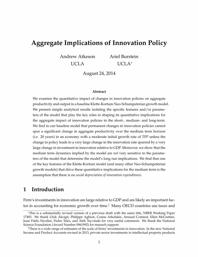
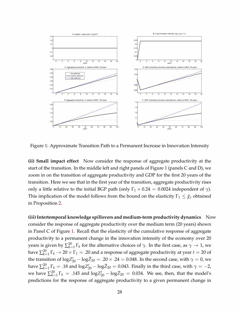
We illustrate our first order approximation to the dynamics of the transition for ourmodel economy in Figure 1. In constructing this figure, as shown in Panel A, we assumethat on this transition path, the physical capital to output ratio is constant at its BGPlevel. As shown in Panel B, we also assume that that the innovation intensity of theeconomy jumps to its new BGP level immediately, i.e. log s′rt − log sr = .24 for all t ≥ 0.We do so to illustrate the quantitative implications of the model given a specified pathfor the innovation intensity of the economy. In the next section, we compute the fullmodel to examine the actual transition path for the innovation intensity and physicalcapital to output ratio of the economy given our specific policy experiment to evaluatethe usefulness of these approximations. We now use this example to discuss four mainquantitative implications of our analytical results.

(i) Intertemporal knowledge spillovers and long run elasticities In the bottom leftand right panels of Figure 1 (panels E and F) we show the transition paths for aggregateproductivity and GDP, both as ratios to their levels on the initial BGP for the first 100years of the transition. From Corollary 1, we have that the response of aggregate produc-tivity in the long-run is very sensitive to the choice of intertemporal knowledge spilloverparameter γ. As γ → 1, the response of aggregate productivity becomes infinite becausethe growth rate of aggregate productivity is approximately Γ1(log s′r − log sr) = 0.0024(24 basis points) above its initial level permanently (in the limit). In contrast, if γ = 0,then the long run response of aggregate productivity relative to its initial BGP path isLp × .24 = .2 so productivity is up only 20% relative to its level on the initial BGP in thelong run. More striking, if γ = −2, then aggregate productivity rises only 6.7% relativeto its initial BGP path in the long run. Using the formula for the dynamics of GDP un-der the assumption that the physical capital to output ratio remains constant obtained inCorollary 2, we see that the response of GDP in the long run is also very sensitive to thechoice of intertemporal knowledge spillover parameter.

27

0 2 4 6 8 10 12 14 16 18 20

−0.2

−0.1

0

0.1

0.2

0.3

A: Capital / output ratio, ∆ log K/Y

years0 2 4 6 8 10 12 14 16 18 20

0

0.05

0.1

0.15

0.2

0.25

B: ∆ log innovation intensity, log ( sr/s

r(−1) )

years

0 2 4 6 8 10 12 14 16 18 201

1.01

1.02

1.03

1.04

1.05

1.06C: Aggregate productivity, Z, relative to BGP, 20 years

low spillovers

medium spillovers

high spillovers

0 2 4 6 8 10 12 14 16 18 20

0.96

0.98

1

1.02

1.04D: GDP (excluding innovation expenditures), relative to BGP, 20 years

0 10 20 30 40 50 60 70 80 90 1001

1.05

1.1

1.15

1.2

1.25

years

E: Aggregate productivity, Z, relative to BGP, 100 years

0 10 20 30 40 50 60 70 80 90 100

1

1.1

1.2

1.3

1.4

years

F: GDP (excluding innovation expenditures), relative to BGP, 100 years

Figure 1: Approximate Transition Path to a Permanent Increase in Innovation Intensity

(ii) Small impact effect Now consider the response of aggregate productivity at thestart of the transition. In the middle left and right panels of Figure 1 (panels C and D), wezoom in on the transition of aggregate productivity and GDP for the first 20 years of thetransition. Here we see that in the first year of the transition, aggregate productivity risesonly a little relative to the initial BGP path (only Γ1 × 0.24 = 0.0024 independent of γ).This implication of the model follows from the bound on the elasticity Γ1 ≤ gz obtainedin Proposition 2.

(iii) Intertemporal knowledge spillovers and medium-term productivity dynamics Nowconsider the response of aggregate productivity over the medium term (20 years) shownin Panel C of Figure 1. Recall that the elasticity of the cumulative response of aggregateproductivity to a permanent change in the innovation intensity of the economy over 20years is given by ∑20

k=1 Γk for the alternative choices of γ. In the first case, as γ → 1, wehave ∑20

k=1 Γk → 20× Γ1 = .20 and a response of aggregate productivity at year t = 20 ofthe transition of logZ′20 − logZ20 = .20× .24 = 0.048. In the second case, with γ = 0, wehave ∑20

k=1 Γk = .18 and logZ′20 − logZ20 = 0.043. Finally in the third case, with γ = −2,we have ∑20

k=1 Γk = .145 and logZ′20 − logZ20 = 0.034. We see, then, that the model’spredictions for the response of aggregate productivity to a given permanent change in

28

the innovation intensity of the economy 20 years into the transition are not particularlysensitive to choices of the intertemporal knowledge spillover parameter γ in comparisonto the strong dependence of the model’s long run predictions for aggregate productivityon this parameter.

(iv) Output gains are in the long run Next consider the transition path for GDP ex-clusive of innovation expenditures (resources available for consumption and physical in-vestment) shown in panel D of Figure 1. In that figure, we see that GDP falls considerablyon impact, regains its initial level in roughly 10 years, and is only modestly above its ini-tial level in 20 years. Moreover, we see that the path of GDP in these first 20 years isnot particularly sensitive to the choice of the knowledge spillover parameter γ. Recallfrom Proposition 2 and Corollary 2 that, holding fixed the rental rate of physical capital,the elasticity of GDP at horizon t with respect to a permanent change in the innovationintensity of the economy is given by

log GDP′t − log ¯GDPt

log s′r − log sr=

(t

∑k=1

Γk1− α

− Lr

).

In our calibration, this term is equal to −Lr = −.167 on impact at t = 0. With γ → 1,this elasticity approaches .133 at t = 20, while with γ = −2, it is .051 at t = 20. Inour particular policy experiment, since the log change in the innovation intensity of theeconomy is .24, the log change in GDP excluding innovation expenditures is 0.032 at t =20 with γ → 1 and only 0.012 at t = 20 with γ = −2. Recall that to convert these resultsto implications for GDP inclusive of innovation expenditure one must multiply the levelof GDP exclusive of these expenditures by (1 + srt).

This result that our model’s implications for the medium term elasticity of aggregateproductivity and GDP with respect to a permanent change in innovation policies is rela-tively small for a wide range of values of the intertemporal knowledge spillover param-eter γ does not imply that the current equilibrium level of innovation expenditures isclose to optimal. In fact, from equation (35), we have that, for a wide range of values ofconsumers’ discount factor β and of the intertemporal knowledge spillover parametersγ, our model implies that the optimal BGP innovation intensity of the economy is higherthan the initial level we have assumed. Specifically, using our parameter values above,we have Γ∗1/L∗p = σΦ 1

ρ−1exp((ρ−1)gz)−1

exp((ρ−1)gz)= 0.012. Equation (35) then implies that with

β = .99 (the real interest rate is one percentage point higher then the growth rate) andγ = .99 (close to endogenous growth), the optimal innovation intensity of the economyis s∗r = 1.18, that is, innovation expenditures should exceed expenditure on consump-

29

tion and physical investment combined by 18%. On the conservative side, with impatientconsumers (β = .96) and low intertemporal knowledge spillovers (γ = −2), s∗r = 0.155, afigure that is not too far from the measures of investments in intangible capital relative toGDP calculated by Corrado et al. (2009).

Clearly, our model’s implications for the optimal innovation intensity of the economyare highly sensitive to assumptions about consumers’ patience β and the level of intertem-poral knowledge spillovers γ. Moreover, the model’s implications for the optimal inno-vation intensity of the economy are not particularly sensitive to other parameters, giventhat we know that the term Γ1/Lp must be bounded be the value of gz that we match incalibrating the model.

Sensitivity to alternative parameter choices Our characterization of our model’s dy-namics using simple first order approximations is useful for highlighting which featuresof the model are important in determining its quantitative implications and for under-standing quantitatively the sensitivity of these implications with respect to these modelfeatures. For example, consider the impact of calibrating the model to a higher level ofproductivity growth gz on the initial BGP. If we double this initial level of productivitygrowth, holding other parameters fixed (except for gAr , which we modify to be consistentwith this higher growth rate), then from expression (19) the upper bound on the elasticityof aggregate productivity on impact Γ1 also doubles. The change in the exact value of Γ1

depends on the value of ρ: for ρ close to 1, Γ1 also doubles; as ρ approaches infinity, thevalue of Γ1 becomes insensitive to gz. With ρ = 4, doubling gz from .0125 to .025 raises Γ1

from 0.01 to .019. In the case of endogenous growth, γ = 1, the 20-year elasticity of aggre-gate productivity ∑20

k=1 Γk increases from .2 to .39. In the semi-endogenous growth case,γ < 1, the terms Γk decay more quickly, so, in the case with low intertemporal knowledgespillovers γ = −2 that we considered, this medium term elasticity rises from .143 to .212Hence in this case, the elasticities of productivity implied by the model are larger and themedium term implications of the model are more sensitive to changes in the knowledgespillover parameter γ.

Likewise, consider the sensitivity of our results to the calibration of the innovationintensity of the economy sr on the initial BGP. We considered a policy experiment in whichinnovation subsidies are increased in a uniform manner resulting in the long run in achange of fiscal expenditures on these policies of 3 percent of GDP. From Proposition1, we have that the corresponding long-run change in the innovation intensity of theeconomy s′ − sr is also 3 percent of GDP. If we calibrate the model to a lower initial valueof sr on the initial GDP, then, mechanically, our model implies that this policy experiment

30

results in a larger change in the log of the innovation intensity of the economy. Thus,keeping the model elasticities Γk unchanged, the magnitude of the response of aggregateproductivity to this policy experiment will be larger. For example, if we had assumedan initial innovation intensity of the economy of 5 percent in line with the new measuresof intangible investment relative to Private Business Output in the NIPA in recent years,then our policy experiment would have increased the log of the innovation intensity ofthe economy by log .08− log .05 = .47 rather than .24.

Next consider the implications of assuming larger differences between the averagecost of innovation for incumbent and entering firms (c(q) versus c′(q)q). Changes in thisassumption impact the parameter Φ. In our calibration, we have set Φ = .966 close toits maximum value of one. As discussed in Proposition 4, if we choose a smaller valueof Φ, the elasticity of aggregate productivity with respect to a permanent change in theinnovation intensity of the economy is reduced at every horizon, while the implicationsof the model for the long run are unchanged.

Finally, in assuming that σ ≤ 1, we have abstracted from contemporaneous positivespillovers in research effort. Instead, if one assumes that there are increasing contempora-neous returns in the mapping from firms’ research effort to the aggregate innovation rate,one could model these by assuming σ > 1. The impact of this change in assumptions onour model elasticities Γk is straightforward. Assuming a value of σ > 1 raises Γ1 and theelasticity of aggregate productivity to a permanent change in the innovation intensity ofthe economy at any horizon in the same manner that assuming a lower value of Φ reducesthese elasticities.19

Social depreciation of innovation expenditures A striking implication of Proposition2 is that we are able to derive an upper bound on the elasticity of the growth of aggregateproductivity with respect to the innovation intensity of the economy, Γ1, without speci-fying many of the underlying parameters of the model. What is key to determining themagnitude of that bound, however, is the implicit assumption that is made in specify-ing the model regarding the level of aggregate productivity growth that would occur ifoutput of the research good were to be set to zero — a quantity that we term the socialdepreciation of innovation expenditures. Note that in our model there is private depreciationof innovation expenditures. In particular, individual firms perceive that they will losethe profits associated with any successful innovation at the rate δt determined by the in-novation expenditures of other firms. But society does not lose the benefits of this past

19See, for example, Bloom et al. (2013) for estimates of contemporaneous technological spillovers usingU.S. detailed firm level data.

31

innovation as captured in the productivity aggregate Zt.To see the importance of this implicit assumption regarding the social depreciation

of innovation built in to our Neo-Schumpeterian model, consider equation (30) from theproof of Proposition 2. In that equation, from the log concavity of G (δ), defined as Zt+1

Z1=

G(δt), we had the bound on the elasticity of aggregate productivity with respect to theinnovation rate of

log Z′t+1/Z′t − gz

log δ′t − log δ=

G′(δ)

δ

G(δ) ≤ logG

(δ)− logG (0) = gz − logG (0) .

Mechanically, as long as the transition law for aggregate productivity is log concave inthe innovation rate, calibration of the transition law at the BGP innovation rate and at azero innovation rate is sufficient to bound the elasticity of aggregate productivity withrespect to the innovation rate at the BGP. The assumption that aggregate productivityremains constant with an innovation rate of zero (i.e. G(0) = 1) gave us the bound onthis elasticity of gz.

Consider the implications of the alternative assumption that aggregate productivitywould decline if the innovation rate were zero. Specifically, let Zt+1

Zt= G(0) < 1 be the

gross growth rate of aggregate productivity if the innovation rate is equal to zero. Thenthe elasticity of aggregate productivity with respect to the innovation rate is bounded by anumber larger than gz. Moreover, by direct calculation of this elasticity using the specificfunctional form for G (δ) in our baseline Klette-Kortum model (see equation (31)) we seethat with social depreciation of innovation this elasticity is in fact larger. For example,if we assume that aggregate productivity would decline by 3.5% if the innovation ratewas zero (G (0) = 0.965) then with ρ = 4 and G(δ) = 1.0125, this elasticity is 0.044(and the upper bound above is 0.048) rather than 0.0123 (and an upper bound of 0.0125).Thus, with a moderate social depreciation rate of innovation of 3.5% per year, we obtainan elasticity of aggregate productivity growth with respect to the innovation rate thatis roughly three and a half times larger than what we obtain in the absence of socialdepreciation.

With this assumption, together with our initial calibration of σ, Φ, and Lp, we getΓ1 = .036 rather than the value of Γ1 = .01 that we obtained under the assumption of nosocial depreciation of innovation. This implies that with high intertemporal knowledgespillovers (γ → 1) the medium term elasticity of aggregate productivity with respect toa permanent change in the innovation intensity of the economy is ∑20

k=1 Γk = .72 ratherthan 0.2 with no social depreciation of innovation. With low intertemporal knowledgespillovers (γ = −2), this elasticity is ∑20

k=1 Γk = .26 rather than .14 with no social depreci-

32

ation of innovation. On the other hand, ∑∞k=1 Γk =

Lp1−γ , which determines the long-term

change (across BGPs) in aggregates, is independent of the social rate of depreciation.These results imply that in an economy with a moderate initial TFP growth rate and

with a modest social depreciation of innovation, the medium term elasticity of aggregateproductivity with respect to a permanent change in the innovation intensity of the econ-omy is both significantly larger than it is with no social depreciation of innovation andmuch more sensitive to the magnitude of intertemporal knowledge spillovers. In particu-lar, with significant social depreciation of innovation and high intertemporal knowledgespillovers, we have from Corollary 2 that measured GDP exclusive of innovation expen-ditures rises relative to its initial BGP path after only 5 years of transition following apermanent increase in the innovation intensity of the economy instead of after more than10 years as shown in panel D of Figure 1.

Note as well that the faster transition dynamics for measured GDP that one obtainswhen one assumes that there is social depreciation of innovation expenditures also hasnormative implications. Specifically, with social depreciation of innovation expenditures,Γ1/Lp rises (holding fixed all other parameters and policies) and hence from equation(35), the optimal innovation intensity of the economy also rises.

The importance of social depreciation of innovation in determining an upper boundon the elasticity of productivity growth with respect to output of the research good thatwe derive is not specific to the Quality Ladders/Klette Kortum type model consideredhere. For example, it applies as well to the growth model in Jones (2002) in which thegrowth of aggregate productivity can be written directly as a function of output of theresearch good Yrt

Zt+1

Zt= H(Yrt),

where logH is an increasing and concave function of research output.20 Here, the elastic-ity of aggregate productivity growth with respect to research output is given by

log Z′t+1/Z′t − gz

log Yrt − log Yr=

H′(Yr)Yr

H(Yr)≤ logH(Yr)− logH(0),

where the inequality follows from the concavity of logH with respect to research output.In Jones (2002), it is assumed that there is no social depreciation of innovation, so H(0) =1 and this elasticity is bounded above by gz. On the other hand, if one assumes that thereis social depreciation of innovation, i.e. H(0) < 1, this elasticity can be larger.

20The transition law for aggregate productivity is given in equation (5) in Jones (2002). We interpret theexpression on the right hand side of that equation as output of the research good.

33

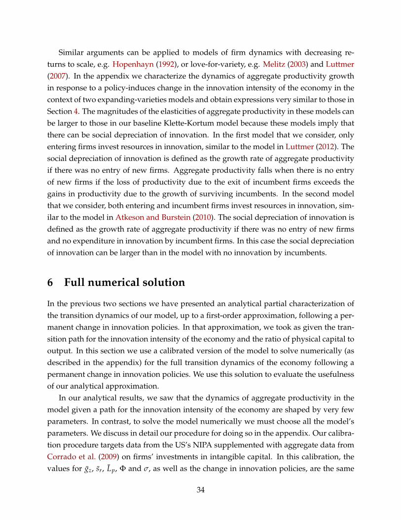
Similar arguments can be applied to models of firm dynamics with decreasing re-turns to scale, e.g. Hopenhayn (1992), or love-for-variety, e.g. Melitz (2003) and Luttmer(2007). In the appendix we characterize the dynamics of aggregate productivity growthin response to a policy-induces change in the innovation intensity of the economy in thecontext of two expanding-varieties models and obtain expressions very similar to those inSection 4. The magnitudes of the elasticities of aggregate productivity in these models canbe larger to those in our baseline Klette-Kortum model because these models imply thatthere can be social depreciation of innovation. In the first model that we consider, onlyentering firms invest resources in innovation, similar to the model in Luttmer (2012). Thesocial depreciation of innovation is defined as the growth rate of aggregate productivityif there was no entry of new firms. Aggregate productivity falls when there is no entryof new firms if the loss of productivity due to the exit of incumbent firms exceeds thegains in productivity due to the growth of surviving incumbents. In the second modelthat we consider, both entering and incumbent firms invest resources in innovation, sim-ilar to the model in Atkeson and Burstein (2010). The social depreciation of innovation isdefined as the growth rate of aggregate productivity if there was no entry of new firmsand no expenditure in innovation by incumbent firms. In this case the social depreciationof innovation can be larger than in the model with no innovation by incumbents.

6 Full numerical solution

In the previous two sections we have presented an analytical partial characterization ofthe transition dynamics of our model, up to a first-order approximation, following a per-manent change in innovation policies. In that approximation, we took as given the tran-sition path for the innovation intensity of the economy and the ratio of physical capital tooutput. In this section we use a calibrated version of the model to solve numerically (asdescribed in the appendix) for the full transition dynamics of the economy following apermanent change in innovation policies. We use this solution to evaluate the usefulnessof our analytical approximation.

In our analytical results, we saw that the dynamics of aggregate productivity in themodel given a path for the innovation intensity of the economy are shaped by very fewparameters. In contrast, to solve the model numerically we must choose all the model’sparameters. We discuss in detail our procedure for doing so in the appendix. Our calibra-tion procedure targets data from the US’s NIPA supplemented with aggregate data fromCorrado et al. (2009) on firms’ investments in intangible capital. In this calibration, thevalues for gz, sr, Lp, Φ and σ, as well as the change in innovation policies, are the same

34

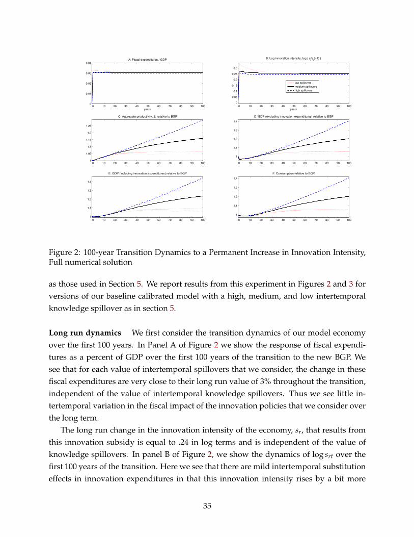
0 10 20 30 40 50 60 70 80 90 1000

0.01

0.02

0.03

0.04A: Fiscal expenditures / GDP

years0 10 20 30 40 50 60 70 80 90 100

0

0.05

0.1

0.15

0.2

0.25

0.3

B: Log innovation intensity, log ( sr/s

r(−1) )

years

low spillovers

medium spillovers

high spillovers

0 10 20 30 40 50 60 70 80 90 1001

1.05

1.1

1.15

1.2

1.25

C: Aggregate productivity, Z, relative to BGP

0 10 20 30 40 50 60 70 80 90 100

1

1.1

1.2

1.3

1.4

D: GDP (excluding innovation expenditures) relative to BGP

0 10 20 30 40 50 60 70 80 90 1001

1.1

1.2

1.3

1.4

E: GDP (including innovation expenditures) relative to BGP

0 10 20 30 40 50 60 70 80 90 100

1

1.1

1.2

1.3

1.4

F: Consumption relative to BGP

Figure 2: 100-year Transition Dynamics to a Permanent Increase in Innovation Intensity,Full numerical solution

as those used in Section 5. We report results from this experiment in Figures 2 and 3 forversions of our baseline calibrated model with a high, medium, and low intertemporalknowledge spillover as in section 5.

Long run dynamics We first consider the transition dynamics of our model economyover the first 100 years. In Panel A of Figure 2 we show the response of fiscal expendi-tures as a percent of GDP over the first 100 years of the transition to the new BGP. Wesee that for each value of intertemporal spillovers that we consider, the change in thesefiscal expenditures are very close to their long run value of 3% throughout the transition,independent of the value of intertemporal knowledge spillovers. Thus we see little in-tertemporal variation in the fiscal impact of the innovation policies that we consider overthe long term.

The long run change in the innovation intensity of the economy, sr, that results fromthis innovation subsidy is equal to .24 in log terms and is independent of the value ofknowledge spillovers. In panel B of Figure 2, we show the dynamics of log srt over thefirst 100 years of the transition. Here we see that there are mild intertemporal substitutioneffects in innovation expenditures in that this innovation intensity rises by a bit more

35

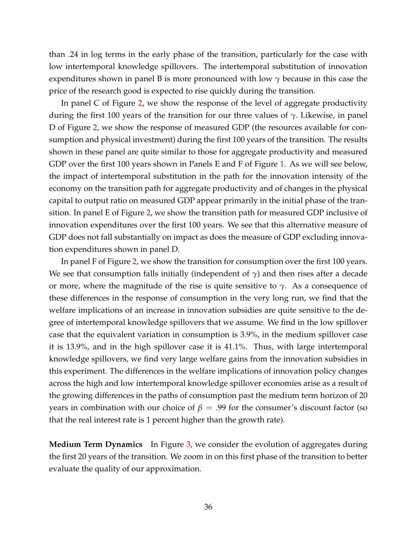
than .24 in log terms in the early phase of the transition, particularly for the case withlow intertemporal knowledge spillovers. The intertemporal substitution of innovationexpenditures shown in panel B is more pronounced with low γ because in this case theprice of the research good is expected to rise quickly during the transition.

In panel C of Figure 2, we show the response of the level of aggregate productivityduring the first 100 years of the transition for our three values of γ. Likewise, in panelD of Figure 2, we show the response of measured GDP (the resources available for con-sumption and physical investment) during the first 100 years of the transition. The resultsshown in these panel are quite similar to those for aggregate productivity and measuredGDP over the first 100 years shown in Panels E and F of Figure 1. As we will see below,the impact of intertemporal substitution in the path for the innovation intensity of theeconomy on the transition path for aggregate productivity and of changes in the physicalcapital to output ratio on measured GDP appear primarily in the initial phase of the tran-sition. In panel E of Figure 2, we show the transition path for measured GDP inclusive ofinnovation expenditures over the first 100 years. We see that this alternative measure ofGDP does not fall substantially on impact as does the measure of GDP excluding innova-tion expenditures shown in panel D.

In panel F of Figure 2, we show the transition for consumption over the first 100 years.We see that consumption falls initially (independent of γ) and then rises after a decadeor more, where the magnitude of the rise is quite sensitive to γ. As a consequence ofthese differences in the response of consumption in the very long run, we find that thewelfare implications of an increase in innovation subsidies are quite sensitive to the de-gree of intertemporal knowledge spillovers that we assume. We find in the low spillovercase that the equivalent variation in consumption is 3.9%, in the medium spillover caseit is 13.9%, and in the high spillover case it is 41.1%. Thus, with large intertemporalknowledge spillovers, we find very large welfare gains from the innovation subsidies inthis experiment. The differences in the welfare implications of innovation policy changesacross the high and low intertemporal knowledge spillover economies arise as a result ofthe growing differences in the paths of consumption past the medium term horizon of 20years in combination with our choice of β = .99 for the consumer’s discount factor (sothat the real interest rate is 1 percent higher than the growth rate).

Medium Term Dynamics In Figure 3, we consider the evolution of aggregates duringthe first 20 years of the transition. We zoom in on this first phase of the transition to betterevaluate the quality of our approximation.

36

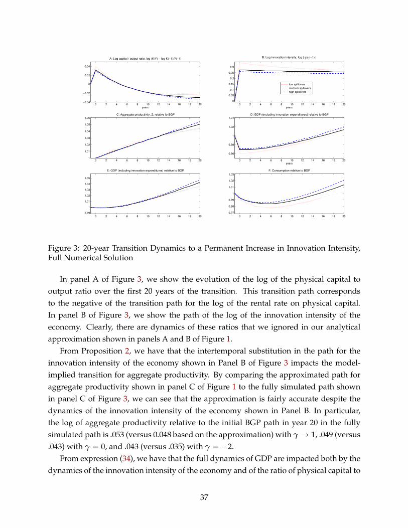
0 2 4 6 8 10 12 14 16 18 20−0.04

−0.02

0

0.02

0.04

A: Log capital / output ratio, log (K/Y) − log K(−1)/Y(−1)

years0 2 4 6 8 10 12 14 16 18 20

0

0.05

0.1

0.15

0.2

0.25

0.3

B: Log innovation intensity, log ( sr/s

r(−1) )

years

0 2 4 6 8 10 12 14 16 18 201

1.01

1.02

1.03

1.04

1.05

1.06C: Aggregate productivity, Z, relative to BGP

0 2 4 6 8 10 12 14 16 18 20

0.96

0.98

1

1.02

1.04D: GDP (excluding innovation expenditures) relative to BGP

years

0 2 4 6 8 10 12 14 16 18 20

0.99

1

1.01

1.02

1.03

1.04

1.05

E: GDP (including innovation expenditures) relative to BGP

0 2 4 6 8 10 12 14 16 18 20

0.97

0.98

0.99

1

1.01

1.02

1.03

F: Consumption relative to BGP

low spillovers

medium spillovers

high spillovers

Figure 3: 20-year Transition Dynamics to a Permanent Increase in Innovation Intensity,Full Numerical Solution

In panel A of Figure 3, we show the evolution of the log of the physical capital tooutput ratio over the first 20 years of the transition. This transition path correspondsto the negative of the transition path for the log of the rental rate on physical capital.In panel B of Figure 3, we show the path of the log of the innovation intensity of theeconomy. Clearly, there are dynamics of these ratios that we ignored in our analyticalapproximation shown in panels A and B of Figure 1.

From Proposition 2, we have that the intertemporal substitution in the path for theinnovation intensity of the economy shown in Panel B of Figure 3 impacts the model-implied transition for aggregate productivity. By comparing the approximated path foraggregate productivity shown in panel C of Figure 1 to the fully simulated path shownin panel C of Figure 3, we can see that the approximation is fairly accurate despite thedynamics of the innovation intensity of the economy shown in Panel B. In particular,the log of aggregate productivity relative to the initial BGP path in year 20 in the fullysimulated path is .053 (versus 0.048 based on the approximation) with γ→ 1, .049 (versus.043) with γ = 0, and .043 (versus .035) with γ = −2.

From expression (34), we have that the full dynamics of GDP are impacted both by thedynamics of the innovation intensity of the economy and of the ratio of physical capital to

37

output. On impact, these two factors have opposite effects on GDP — the initial increasein the ratio of physical capital to output raise GDP while the initial increase in the inno-vation intensity of the economy above its new long-run level lowers GDP. By comparingthe approximated path for GDP shown in panel D of Figure 1 to the fully simulated pathshown in panel D of Figure 3, we again can see that the approximation is fairly accuratedespite the fact that we ignored the dynamics in the innovation intensity of the economyand the capital-output ratio.

In panels E and F of Figure 3, we show the path of GDP inclusive of innovation expen-ditures and of consumption during the first 20 years of the transition. We see here thatconsumption falls initially for at least 10 years during the transition indicating that thepotentially large welfare gains are achieved only in the long run.

Figure 3 shows that a large and persistent increase in innovation subsidies has a rela-tively small impact on aggregate productivity and GDP over a 20 year horizon, and theresponse of aggregates does not vary much with the extent of intertemporal knowledgespillovers assumed in the model.

These results suggest that it would be hard to verify whether innovation policies yieldlarge output and welfare gains using medium term data on the response of aggregates tochanges in innovation policies. We illustrate this point in Figure 4. In that figure we showresults obtained from simulating the response of aggregates in our model to our baselineincrease in innovation subsidies in a version of our model with Hicks neutral AR1 pro-ductivity shocks Apt with a persistence of 0.9 and an annual standard deviation of 2%.We introduce these shocks as a proxy for business cycle shocks around the BGP. We showhistograms generated from 3000 simulations of the model for the first 20 years of the tran-sition. The units on the horizontal axis show the log of the ratio of detrended GDP at theend of the 20th year of transition to initial GDP and the vertical axis shows the frequencyof the corresponding outcome for GDP. In panel A of the figure, we show results for GDPexcluding innovation expenditures. In panel B, we show results for GDP including in-novation expenditures. The red bars show results for the model with low intertemporalknowledge spillovers and the blue bars show the results with high spillovers. Clearly,in each panel, the distribution represented by the blue bars is slightly to the right of thatrepresented by the red bars. The histograms in panel B are shifted to the right relativeto those in panel A reflecting the fact that GDP including innovation expenditures has ahigher elasticity of changes in the innovation intensity of the economy. But it is also clearin each panel that, using either measure of GDP, that it would be very hard to distinguishthe degree of intertemporal knowledge spillovers (and, hence, the long term effects fromthis innovation subsidy) in aggregate time series data even if we had the benefit of a true

38

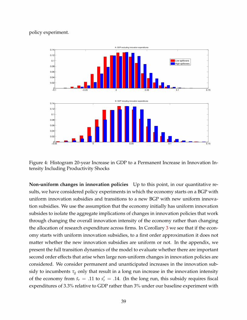
policy experiment.

−0.1 −0.05 0 0.05 0.1 0.150

0.02

0.04

0.06

0.08

0.1

0.12

0.14A: GDP excluding innovation expenditures

Low spillovers

High spillovers

−0.05 0 0.05 0.1 0.150

0.02

0.04

0.06

0.08

0.1

0.12

0.14B: GDP including innovation expenditures

Figure 4: Histogram 20-year Increase in GDP to a Permanent Increase in Innovation In-tensity Including Productivity Shocks

Non-uniform changes in innovation policies Up to this point, in our quantitative re-sults, we have considered policy experiments in which the economy starts on a BGP withuniform innovation subsidies and transitions to a new BGP with new uniform innova-tion subsidies. We use the assumption that the economy initially has uniform innovationsubsides to isolate the aggregate implications of changes in innovation policies that workthrough changing the overall innovation intensity of the economy rather than changingthe allocation of research expenditure across firms. In Corollary 3 we see that if the econ-omy starts with uniform innovation subsidies, to a first order approximation it does notmatter whether the new innovation subsidies are uniform or not. In the appendix, wepresent the full transition dynamics of the model to evaluate whether there are importantsecond order effects that arise when large non-uniform changes in innovation policies areconsidered. We consider permanent and unanticipated increases in the innovation sub-sidy to incumbents τg only that result in a long run increase in the innovation intensityof the economy from sr = .11 to s′r = .14. (In the long run, this subsidy requires fiscalexpenditures of 3.3% relative to GDP rather than 3% under our baseline experiment with

39

uniform innovation policies). We show these dynamics for economies with two differentcurvatures of the incumbents’ innovation cost function, c(q), which determines the elas-ticity of innovation effort, q, with respect to the incentives to innovate. We consider aninelastic case in which the share of innovative effort by incumbents, q/(q + M), acrossthe old and new BGP is constant at our baseline level of 75%, and an elastic case in whichthe share of innovative effort by incumbents increases significantly across old and newBGPs from 75% to 96% (implying a substantial fall in the share of employment in newfirms). We find in both cases that our first order approximation is fairly accurate in thatthe dynamics of aggregate productivity and measured GDP are not much different thanthose that we found with uniform changes in innovation policies.

7 Conclusion

In this paper, we have derived a simple first-order approximation to the transition dy-namics of aggregate productivity and GDP in response to a permanent policy-inducedchange in the innovation intensity of the economy implied by a baseline Klette-Kortummodel. Our results highlight the tight connection between the model’s quantitative im-plications for the transition dynamics for aggregate productivity and GDP following asustained change in innovation policies and the implicit assumption one makes regardingthe social depreciation of innovation in specifying the model. If one assumes that thereis no social depreciation of innovation, then in using this model to analyze changes ininnovation policies in advanced economies (with relatively slow baseline growth rates ofproductivity), one is driven to the conclusion that changes in innovation policies wouldonly pay off in terms of sustained increases in productivity, output, and consumptionafter 10 years or more, regardless of the other parameters of the model. Under this as-sumption, such policy changes could lead to substantial welfare gains only if consumersare patient and willing to wait for boost in consumption several decades in exchange fora reduction in consumption today. In contrast, if one assumes that there is substantialsocial depreciation of innovation, then one opens up the possibility that a change in in-novation policies could have a significantly larger payoff in the medium term in terms ofincreased productivity, output, and consumption. These results indicate the importanceof improving our modeling and measurement of the social rather than private deprecia-tion of innovation.

The analytical approach that we have taken here to characterizing our model’s tran-sition dynamics is also useful for examining related questions such as the implicationsof changes in the patent rate and/or changes in the firm startup rate as measured by the

40

share of labor employed in young firms for the dynamics of aggregate productivity. See,for example Kogan et al. (2012) for a study of patent based measures of the innovationrate and Decker et al. (2013) for a study of changes in the firms’ startup rate in the U.S.In choosing a model to analyze these questions, implicit assumptions about the social de-preciation of innovation should also play an important role in shaping the quantitativeresults of the analysis.

Finally, under our baseline assumptions, we have abstracted from the productivityand welfare gains that might be achieved by reallocating a given level of investment ininnovation across heterogeneous firms. Under alternative settings in which there are first-order gains from such a reallocation, one may wish to consider a whole range of policiesaimed at reallocating innovation expenditures across firms. The research challenge hereis to find reliable metrics for evaluating which firms should be doing more investment ininnovation and which should be doing less. Regardless, it is likely that in such extensionsof our baseline model, the social depreciation of innovation will still be an importantparameter shaping the quantitative results.

ReferencesAcemoglu, Daron, “Introduction to Modern Economic Growth,” 2009.

, Ufuk Akcigit, Nicholas Bloom, and William R. Kerr, “Innovation, Reallocation and Growth,”NBER Working Papers 18993, National Bureau of Economic Research, Inc April 2013.

Aghion, Philippe and Peter Howitt, “A Model of Growth through Creative Destruction,” Econo-metrica, March 1992, 60 (2), 323–51.

, Ufuk Akcigit, and Peter Howitt, “What Do We Learn From Schumpeterian Growth Theory?,”February 2013, (298).

Aizcorbe, Ana, Carol Moylan, and Carol Robbins, “Toward Better Measurement of Innovationand Intangibles,” BEA Briefing, Bureau of Economic Analysis U.S. Department of Commerce2009.

Akcigit, Ufuk and William R. Kerr, “Growth Through Heterogeneous Innovations,” November2010, (16443).

, Douglas Hanley, and Nicolas Serrano-Velarde, “Back to Basics: Basic Research Spillovers,Innovation Policy and Growth,” NBER Working Papers 19473, National Bureau of EconomicResearch, Inc September 2013.

Arkolakis, Costas, Arnaud Costinot, and Andres Rodriguez-Clare, “New Trade Models, SameOld Gains?,” American Economic Review, February 2012, 102 (1), 94–130.

Atkeson, Andrew and Ariel Tomas Burstein, “Innovation, Firm Dynamics, and InternationalTrade,” Journal of Political Economy, 06 2010, 118 (3), 433–484.

41

Bloom, Nicholas, Mark Schankerman, and John Van Reenen, “Identifying Technology Spilloversand Product Market Rivalry,” Econometrica, 07 2013, 81 (4), 1347–1393.

Buera, Francisco and Roberto Fattal-Jaef, “The Dynamics of Development: Entrepreneurship,Innovation, and Reallocation,” Working Paper, World Bank 2014.

Comin, Diego and Mark Gertler, “Medium-Term Business Cycles,” American Economic Review,June 2006, 96 (3), 523–551.

Corrado, Carol A. and Charles R. Hulten, “Innovation Accounting,” in “Measuring EconomicSustainability and Progress” NBER Chapters, National Bureau of Economic Research, Inc, De-cember 2013.

Corrado, Carol, Charles Hulten, and Daniel Sichel, “Measuring Capital and Technology: AnExpanded Framework,” in “Measuring Capital in the New Economy” NBER Chapters, NationalBureau of Economic Research, Inc, December 2005, pp. 11–46.

, , and , “Intangible Capital And U.S. Economic Growth,” Review of Income and Wealth, 092009, 55 (3), 661–685.

, Peter Goodridge, and Jonathan Haskel, “Constructing a Price Deflator for R&D: Calculatingthe Price of Knowledge Investments as a Residual,” Economics Program Working Papers 11-03,The Conference Board, Economics Program October 2011.

Decker, Ryan, John Haltiwanger, Ron Jarmin, and Javier Miranda, “The Secular Decline in Busi-ness Dynamism in the U.S.,” Working Paper 2013.

Griliches, Zvi, “Issues in Assessing the Contribution of Research and Development to Productiv-ity Growth,” Bell Journal of Economics, Spring 1979, 10 (1), 92–116.

, “The Search for R&D Spillovers,” in “R&D and Productivity: The Econometric Evidence”NBER Chapters, National Bureau of Economic Research, Inc, December 1998, pp. 251–268.

, ed., R&D, Patents and Productivity number 9780226308845. In ‘National Bureau of EconomicResearch Books.’, University of Chicago Press, 1987.

Grossman, Gene M and Elhanan Helpman, “Quality Ladders in the Theory of Growth,” Reviewof Economic Studies, January 1991, 58 (1), 43–61.

Hopenhayn, Hugo A, “Entry, Exit, and Firm Dynamics in Long Run Equilibrium,” Econometrica,September 1992, 60 (5), 1127–50.

Jaimovich, Nir and Sergio Rebelo, “Non-linear Effects of Taxation on Growth,” NBER WorkingPapers 18473, National Bureau of Economic Research, Inc October 2012.

Jones, Charles I., “Sources of U.S. Economic Growth in a World of Ideas,” American EconomicReview, March 2002, 92 (1), 220–239.

and John C. Williams, “Measuring The Social Return To R&D,” The Quarterly Journal of Eco-nomics, November 1998, 113 (4), 1119–1135.

Kendrick, John, “Total Capital and Economic Growth,” Atlantic Economic Journal, 1994, 22 (1),1–18.

42

Klette, Tor Jakob and Samuel Kortum, “Innovating Firms and Aggregate Innovation,” Journal ofPolitical Economy, October 2004, 112 (5), 986–1018.

Kogan, Leonid, Dimitris Papanikolaou, Amit Seru, and Noah Stoffman, “Technological Inno-vation, Resource Allocation, and Growth,” NBER Working Papers 17769, National Bureau ofEconomic Research, Inc January 2012.

Kortum, Samuel S., “Research, Patenting, and Technological Change,” Econometrica, November1997, 65 (6), 1389–1420.

Lentz, Rasmus and Dale T. Mortensen, “An Empirical Model of Growth Through Product Inno-vation,” Econometrica, November 2008, 76 (6), 1317–1373.

Li, Wendy, “Technological Innovation, Resource Allocation, and Growth,” R and D Satellite Ac-count Paper, Bureau of Economic Analysis U.S. Department of Commerce 2012.

Luttmer, Erzo G. J., “Selection, Growth, and the Size Distribution of Firms,” The Quarterly Journalof Economics, 08 2007, 122 (3), 1103–1144.

Luttmer, Erzo G.J., “Slow convergence in economies with firm heterogeneity,” Technical Report2012.

McGrattan, Ellen R. and Edward C. Prescott, “Taxes, Regulations, and the Value of U.S. and U.K.Corporations,” Review of Economic Studies, 2005, 72 (3), 767–796.

and , “On financing retirement with an aging population,” Technical Report 2012.

Melitz, Marc J., “The Impact of Trade on Intra-Industry Reallocations and Aggregate IndustryProductivity,” Econometrica, November 2003, 71 (6), 1695–1725.

Peters, Michael, “Heterogeneous Mark-Ups and Endogenous Misallocation,” Technical Report2013.

Rivera-Batiz, Luis A and Paul M Romer, “Economic Integration and Endogenous Growth,” TheQuarterly Journal of Economics, May 1991, 106 (2), 531–55.

43

A Additional details of BGP, proof of Proposition, and solv-

ing transition dynamics 1

In the body of the paper we described the BGP growth rates and innovation rates. Here we de-

scribe how to solve for other aggregates.

Rescaled Bellman equations: To start, it is useful to present rescaled Bellman equations de-

scribing the value of firms. Defining vt =VtZ

ρ−1t

Prt, ut =

UtPrt

, we have (without imposing BGP),

vt =ΠtZ

ρ−1t

Prt+

(1− δt)

1 + rt

vt+1

exp ((ρ− 1) gzt), (36)

ut = −(1− τg

)c(qt) +

11 + rt

1exp ((ρ− 1) gzt)

qt

qt + Mtδtvt+1 exp (∆)ρ−1 (37)

+1

1 + rt

(qt

qt + Mtδt + 1− δt

)ut+1.

and the free entry condition is

(1− τe) f ≥(

11 + rt

δt

qt + Mt

)(vt+1

exp ((ρ− 1) gzt)exp (∆)ρ−1 + ut+1

), (38)

where 1 + rt = (1 + rt)Prt

Prt+1. In a BGP, the constant in rescaled profits ΠZρ−1/Pr, and values

VZρ−1/Pr, U/Pr are constant over time (as well as r, gz and δ as discussed in the body of the

paper).

Solving other BGP aggregates: The constant ΠZ/Pr is pinned down from the free entry con-

dition as follows. Manipulating equations (36) and (37) and imposing BGP with positive entry, we

can write the free-entry condition (38) as

(1− τe) f M =1

1 + rδ

( qM + 1

) [ξgΠZρ−1

Pr−(1− τg

)c(q)

], (39)

where ξg =r + δ

r exp ((ρ− 1) gz) /exp (∆)ρ−1 + δ≥ 1

and r = β−1 − 1 in the BGP (since in the BGP, Prt falls at a rate gy). Given the value of ΠZρ−1/Pr

that solves this equation, the allocation of labor Lp/Lr is determined as a function of parameters

usingLp

Lr=

(1− α

µ− 1

)ΠZρ−1

Pr

1c (q) + f M

. (40)

44

When γ < 1, the growth rate gz is determined as described in the text (and hence also δ, q and

M). The level of aggregate productivity Z, for a given current value of scientific knowledge Ar,

is determined using equation (8). When γ = 1, one can use the same procedure but instead of

solving for Z (the BGP level of Z, given Ar, is not pinned down), one must solve for the growth

rate gz (and the corresponding values of δ, q and M). The innovation intensity of the economy,

sr, is calculated as a function of parameters using expression (17). Finally, we solve for aggregate

output, Y, using (4), the stock of physical capital, Kt, using the factor shares of physical capital and

production-labor, and consumption, Ct, using (2).

Active innovation by incumbents: We now discuss the condition stated in Section (3) that in

a BGP if incumbents use their innovation technology (i.e. u ≥ 0) then(1− τg

)c (q) /q ≤ (1− τe) f

at the level of q that solves (16). The condition u ≥ 0 (in a BGP) implies

−(1− τg

) c(q)q

+1

1 + r1

q + Mδ[v exp (∆)ρ−1 + u

]≥ 0.

Combining this inequality with the inequality from the free-entry condition, (38), we have

(1− τg

) c (q)q≤ 1

1 + r1

q + Mδ

[v

exp ((ρ− 1) gz)exp (∆)ρ−1 + u

]≤ (1− τe) f

which proves our result.

Proof of Proposition 1: Under the assumption of semi-endogenous growth (γ < 1), δ, gz, r,

and ξg are constant between BGPs. Under uniform innovation policies and firm-entry, M, q and Yr

are constant between BGPs. By equation (39), ΠZρ−1

Pr1

1−τgmust be constant between BGPs. Using

ΠtZρ−1t = µ−1

µ (1 + τs) GDPt and the fact that Yr is constant between BGPs, 1sr(1−τg)

(µ−1)(1+τs)µ

must be unchanged between BGPs. With τs constant between BGPs, we immediately obtain the

first result of the proposition. The second result follows from the fact that with uniform innovation

policies we have EGDP = τgsr + τs, combined with the previous result that sr

(1− τg

)is constant

between BGPs.

Solving transition dynamics In Sections 4 and 5 section we approximated the aggregate tran-

sition taking as given the transition path for the innovation intensity of the economy and the ratio

of physical capital to output. To solve for the path of these two variables for a given change in

policies or other parameters, we solve the model numerically. Specifically, we solve for the path of

Zt, Kt, vt, and ut using the four following Euler equations: (36), (37), (38) and Rkt = dk + rt where

rt =1β

Ct+1Ct− 1. Recall that qt is solved for using equation (16) assuming that there is positive firm

entry (which must be checked). Given a path of Zt and Kt we can solve for all other equilib-

rium outcomes using static equations. We solve for the 4 Euler equations using either standard

45

linearization methods or a shooting algorithm, and we obtain very similar results.

B Calibration

Here we describe the calibration of the model that we use in Sections 5 and 6.

Policies: τs, τg, τe. Given our analytical results, we assume that subsidies to innovation on the

BGP in the data are uniform, so that τe = τg. As a baseline calibration, we set all policies to zero,

but we do indicate in the calibration formulas below where these policies enter.

Interest rate minus growth rate: In our model, on a BGP, the gap between the consumption

interest rate and the growth rate of consumption is determined by the consumers’ discount factor

β. We set this gap to 0.01, which implies β = 1/1.01. Given this choice of discount factor, on the

BGP, the model interest rate in terms of the research good is given by r = 0.01. We set the growth

rate of consumption to gY = .02, which implies a consumption interest rate of r = 0.03. This

calibration of r is consistent with the difference between the interest rate and the consumption

growth rate in McGrattan and Prescott (2012).

Final Consumption Good Production Function: The production function for the final consumption

good is parameterized by ρ, which controls the elasticity of the residual demand curve faced by

intermediate goods producers. In our baseline calibration we set ρ = 4. This elasticity establishes

an upper bound on the markup µ that can be chosen.

Equilibrium Markup: Defining NIPA profits to intangible capital as GDPt− RktKt−WtLt, the share

of these profits in GDP, denoted by πt, is given by

πt = (1 + τs)

(1− 1

µ

)− srt − τs. (41)

From equation (41), the choice of the markup µ is disciplined by data on the innovation intensity

of the economy, sr, and the share of NIPA profits paid to intangible capital relative to GDP. In our

baseline calibration, we target a share of NIPA profits paid to intangible capital in GDP, π, of 1%

from McGrattan and Prescott (2005) and an innovation intensity of the economy, sr, of 11% similar

to the levels estimated by Corrado et al. (2009) for the United States over the last few years. This

implies a markup of 13.6%, µ = 1.136.

Aggregate Production of the Final Consumption Good: Aggregate production of the final consump-

tion good in equation (4) is parameterized by α. We set α = 0.37 to match the observation that the

share of rental payments to physical capital on the BGP, given by (1 + τs)αµ , is equal to 0.33. With

this choice of α, we also have that the share of labor compensation (including production and re-

search) in GDP is given by (1 + τs)1−α

µ + sr = 0.66. The rest of GDP corresponds to profits paid to

intangible capital, π = 1%.

The Allocation of Labor: The equilibrium allocation of labor between production and research is

pinned down in equation (17) by the choices of parameters above and our calibrated innovation

46

intensity of the economy, sr. In our baseline calibration, with sr = .11, we have Lp = .833.

BGP Growth Rates for Scientific Knowledge and Aggregate Productivity: Given our calibration of

per capita GDP growth of 2% and our physical capital share of α, we calibrate the growth rate

of aggregate productivity in the BGP, gz, to 1.25%. For a given choice of γ, the growth rate of

scientific knowledge consistent with these productivity growth rates is given by gAr = (1− γ) gz.

We do not make assumptions about this growth rate directly since we do not observe it. Instead,

we alter this parameter as we vary γ.

Innovation Step Size and BGP Innovation Rate: Our choices of innovation step size ∆ and the

BGP innovation rate δ must be consistent with the BGP growth rate of aggregate productivity for

intermediate firms, gz given in equation 5. We must also have that the innovation step size exceeds

the markup (∆ ≥ µ) to ensure that an incumbent firm has a technological advantage over its latent

competitor consistent with its assumed markup. In our baseline calibration, we set ∆ = ∆l = µ.

Given our choice of elasticity ρ and the implied value of gz, from equation (5), we get then get

δ = 0.08 in our baseline calibration.

Share of innovative effort by entering firms relative to their share of research expenditure: Under the

assumptions on policies made above, the ratio Φ =M/(q + M)

f M/Yris already determined by pa-

rameters that we have previously calibrated (r, δ, and ξg), and by the choice of targets for sr and

π that have been already discussed. To see this, combining the free-entry condition (39) and the

following expression for π/sr under τs = 0,

π

sr=

ΠZρ−1

f MPr−(

c(q)f M + 1

)(

c(q)f M + 1

)we obtain

c (q)f M

=

1−τe1−τg

(1 + r

δ

( qM + 1

))− ξg

1−τg

(1 + π

sr

)ξg

1−τg

(1 + π

sr

)− 1

.

Setting τg = τe = 0,

Φ =

Mq+M

f Mc(q)+ f M

=

c(q)f M + 1qM + 1

=rδ

ξg

(1 + π

sr

)− 1

.

In our baseline calibration, we have Φ = 0.966 so this fraction is close to its upper bound of one,

which means that the average cost of innovation by incumbents is close to the marginal cost of

innovation by incumbents.

Incumbents’ innovation cost function:Our analytic results showed that c (q) does not matter for the first order aggregate effects

of changes in innovation policies (starting from uniform innovation policies) except through Φ.

For the numerical evaluation of our results, we set c (q) = c + φ0qφ. When considering uniform

47

changes in innovation policies, we do not need to specify the curvature parameter φ, because

incumbents do not change their innovation effort q (Moreover, according to Corollary 3, this pa-

rameter does not matter to a first-order approximation even when considering a policy experiment

in which the subsidies to innovation are not uniform). We choose c to target the share of profits in

GDP, π, discussed above. We choose the parameter φ0 so that the level of q in the initial BGP (from

equation (16)) implies a share of employment of entering firms of 3%. In the model, the share of

employment by entering firms is given by

snew =M

q + Mexp((ρ− 1) gz)− (1− δ)

exp((ρ− 1) gz).

This choice of parameters implies that incumbents account for roughly 75% of total innovative

effort. Our baseline results do not depend on the choice of snew as long as we have positive entry

and positive innovation by incumbents. In any calibration of our model, one must check that

incumbents actually want to use their innovation technology (i.e. U > 0). This is the case in our

calibration.

The Intertemporal Knowledge Spillover Parameter γ: Our procedure for calibrating the model to

a given BGP does not discipline the parameter γ. In our policy experiments below, we consider

three alternative values of γ corresponding to a low spillover case (γ = −2), a medium spillover case(γ = 0) and a high spillover case (γ approaching one).

Other parameters: One can show that the parameters f , σ0, and Ar at time 0 can all be normal-

ized to 1 without affecting our results. We abstract from contemporaneous congestion effects in

innovative effort by setting σ = 1. We do this to give our model the best chance of generating fast

transition dynamics.

C Non-uniform changes in innovation policies

We now solve the full transition dynamics of the model to evaluate whether there are impor-

tant second order effects that arise when large non-uniform changes in innovation policies are

considered. We consider permanent and unanticipated increases in the innovation subsidy to in-

cumbents τg only that result in a long run increase in the innovation intensity of the economy from

sr = .11 to s′r = .14. (In the long run, this subsidy requires fiscal expenditures of 3.3% relative to

GDP rather than 3% under our baseline experiment with uniform innovation policies). We show

these dynamics for economies with two different curvatures of the incumbents’ innovation cost

function, c(q), which determines the elasticity of innovation effort, q, with respect to the incentives

to innovate. We consider an inelastic case in which the share of innovative effort by incumbents,

q/(q + M), across the old and new BGP is constant at our baseline level of 75%, and an elastic

case in which the share of innovative effort by incumbents increases significantly across old and

new BGPs from 75% to 96% (implying a substantial fall in the share of employment in new firms).

48

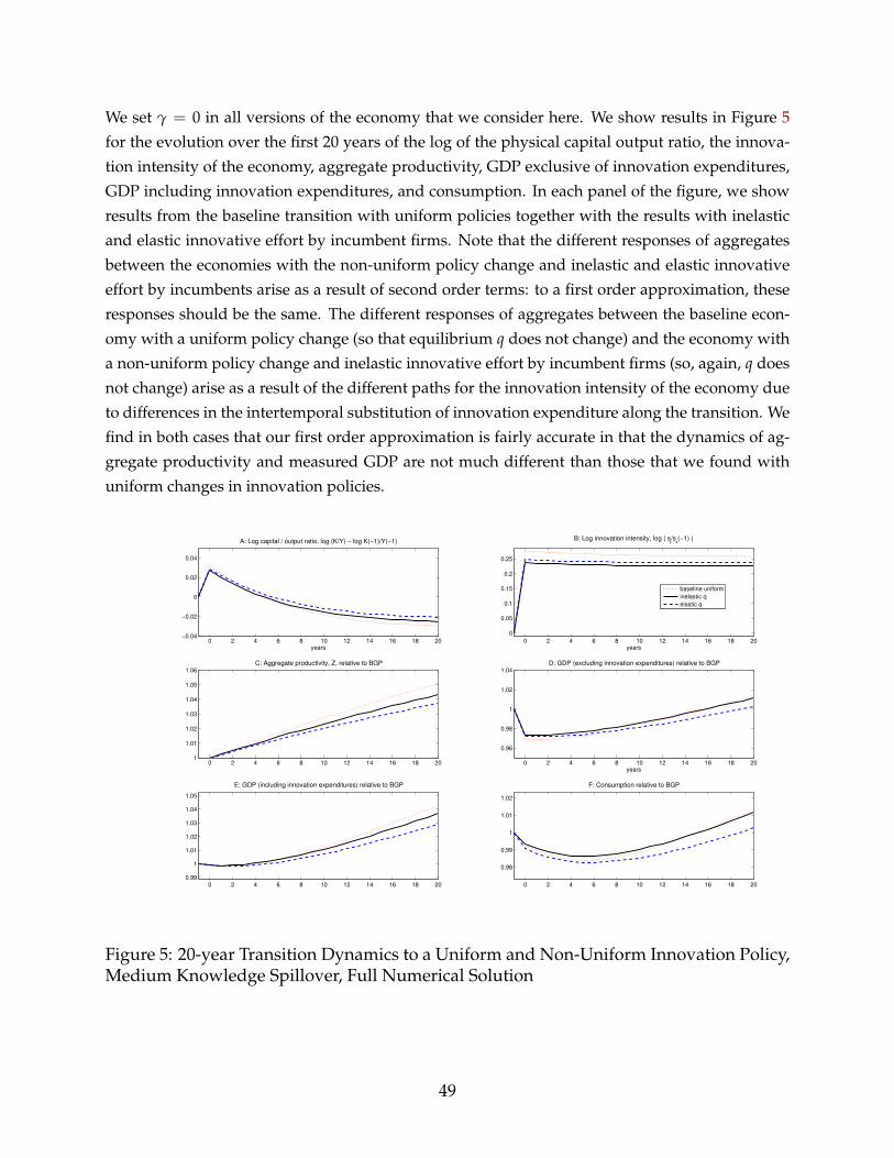
We set γ = 0 in all versions of the economy that we consider here. We show results in Figure 5

for the evolution over the first 20 years of the log of the physical capital output ratio, the innova-

tion intensity of the economy, aggregate productivity, GDP exclusive of innovation expenditures,

GDP including innovation expenditures, and consumption. In each panel of the figure, we show

results from the baseline transition with uniform policies together with the results with inelastic

and elastic innovative effort by incumbent firms. Note that the different responses of aggregates

between the economies with the non-uniform policy change and inelastic and elastic innovative

effort by incumbents arise as a result of second order terms: to a first order approximation, these

responses should be the same. The different responses of aggregates between the baseline econ-

omy with a uniform policy change (so that equilibrium q does not change) and the economy with

a non-uniform policy change and inelastic innovative effort by incumbent firms (so, again, q does

not change) arise as a result of the different paths for the innovation intensity of the economy due

to differences in the intertemporal substitution of innovation expenditure along the transition. We

find in both cases that our first order approximation is fairly accurate in that the dynamics of ag-

gregate productivity and measured GDP are not much different than those that we found with

uniform changes in innovation policies.

0 2 4 6 8 10 12 14 16 18 20−0.04

−0.02

0

0.02

0.04

A: Log capital / output ratio, log (K/Y) − log K(−1)/Y(−1)

years0 2 4 6 8 10 12 14 16 18 20

0

0.05

0.1

0.15

0.2

0.25

B: Log innovation intensity, log ( sr/s

r(−1) )

years

baseline uniform

inelastic q

elastic q

0 2 4 6 8 10 12 14 16 18 201

1.01

1.02

1.03

1.04

1.05

1.06C: Aggregate productivity, Z, relative to BGP

0 2 4 6 8 10 12 14 16 18 20

0.96

0.98

1

1.02

1.04D: GDP (excluding innovation expenditures) relative to BGP

years

0 2 4 6 8 10 12 14 16 18 200.99

1

1.01

1.02

1.03

1.04

1.05

E: GDP (including innovation expenditures) relative to BGP

0 2 4 6 8 10 12 14 16 18 20

0.98

0.99

1

1.01

1.02

F: Consumption relative to BGP

Figure 5: 20-year Transition Dynamics to a Uniform and Non-Uniform Innovation Policy,Medium Knowledge Spillover, Full Numerical Solution

49

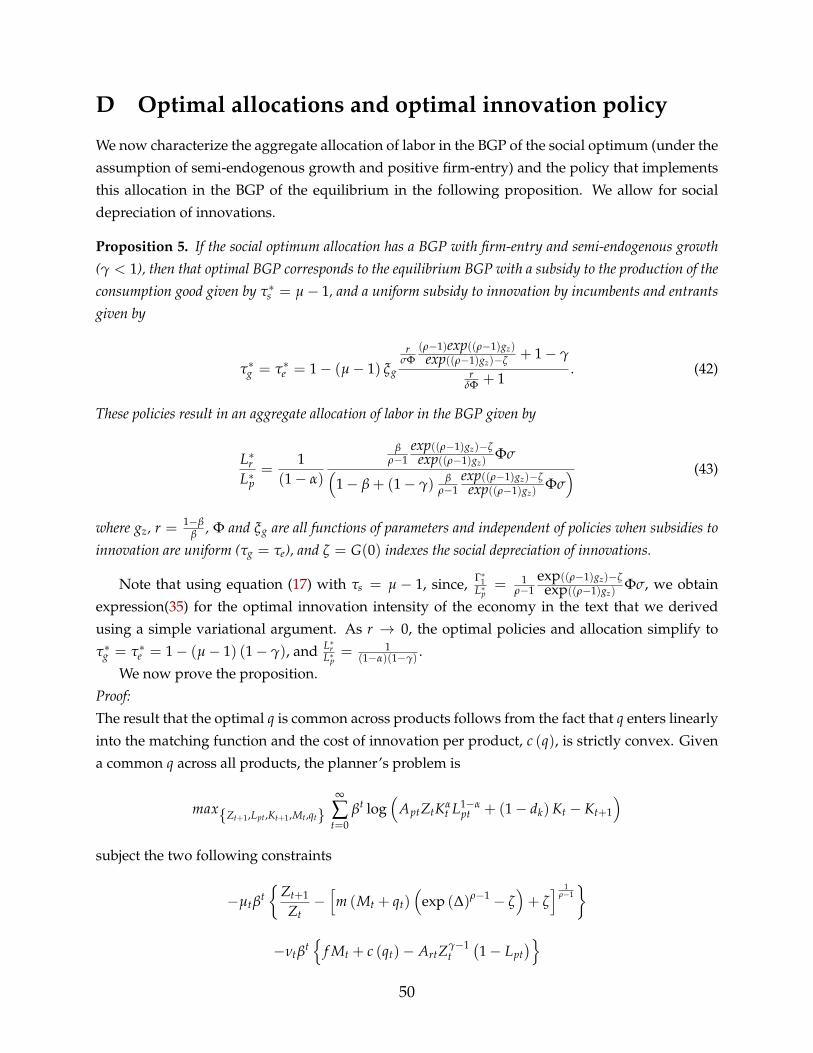
D Optimal allocations and optimal innovation policy

We now characterize the aggregate allocation of labor in the BGP of the social optimum (under the

assumption of semi-endogenous growth and positive firm-entry) and the policy that implements

this allocation in the BGP of the equilibrium in the following proposition. We allow for social

depreciation of innovations.

Proposition 5. If the social optimum allocation has a BGP with firm-entry and semi-endogenous growth(γ < 1), then that optimal BGP corresponds to the equilibrium BGP with a subsidy to the production of theconsumption good given by τ∗s = µ− 1, and a uniform subsidy to innovation by incumbents and entrantsgiven by

τ∗g = τ∗e = 1− (µ− 1) ξg

rσΦ

(ρ−1)exp((ρ−1)gz)

exp((ρ−1)gz)−ζ+ 1− γ

rδΦ + 1

. (42)

These policies result in an aggregate allocation of labor in the BGP given by

L∗rL∗p

=1

(1− α)

βρ−1

exp((ρ−1)gz)−ζ

exp((ρ−1)gz)Φσ(

1− β + (1− γ)β

ρ−1exp((ρ−1)gz)−ζ

exp((ρ−1)gz)Φσ) (43)

where gz, r = 1−ββ , Φ and ξg are all functions of parameters and independent of policies when subsidies to

innovation are uniform (τg = τe), and ζ = G(0) indexes the social depreciation of innovations.

Note that using equation (17) with τs = µ − 1, since, Γ∗1L∗p

= 1ρ−1

exp((ρ−1)gz)−ζ

exp((ρ−1)gz)Φσ, we obtain

expression(35) for the optimal innovation intensity of the economy in the text that we derived

using a simple variational argument. As r → 0, the optimal policies and allocation simplify to

τ∗g = τ∗e = 1− (µ− 1) (1− γ), and L∗rL∗p

= 1(1−α)(1−γ)

.

We now prove the proposition.

Proof:The result that the optimal q is common across products follows from the fact that q enters linearly

into the matching function and the cost of innovation per product, c (q), is strictly convex. Given

a common q across all products, the planner’s problem is

max{Zt+1,Lpt,Kt+1,Mt,qt}∞

∑t=0

βt log(

AptZtKαt L1−α

pt + (1− dk)Kt − Kt+1

)subject the two following constraints

−µtβt{

Zt+1

Zt−[m (Mt + qt)

(exp (∆)ρ−1 − ζ

)+ ζ] 1

ρ−1}

−νtβt{

f Mt + c (qt)− ArtZγ−1t

(1− Lpt

)}50

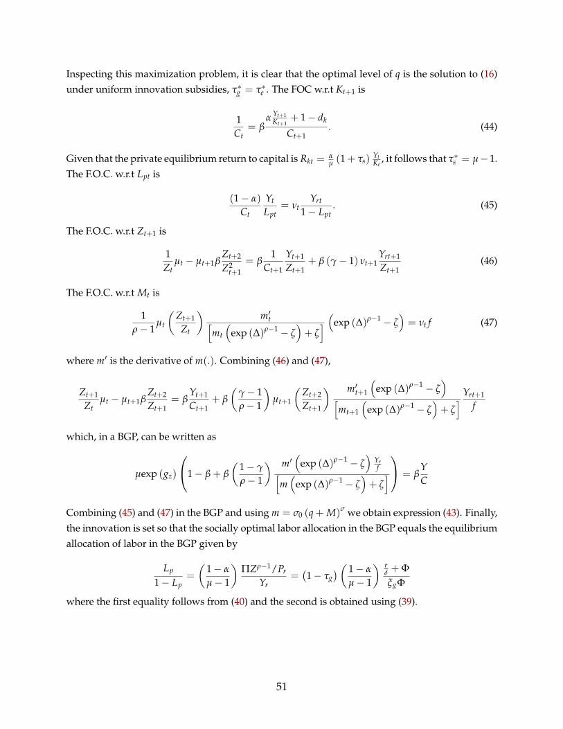
Inspecting this maximization problem, it is clear that the optimal level of q is the solution to (16)

under uniform innovation subsidies, τ∗g = τ∗e . The FOC w.r.t Kt+1 is

1Ct

= βα Yt+1

Kt+1+ 1− dk

Ct+1. (44)

Given that the private equilibrium return to capital is Rkt =αµ (1 + τs)

YtKt

, it follows that τ∗s = µ− 1.

The F.O.C. w.r.t Lpt is

(1− α)

Ct

Yt

Lpt= νt

Yrt

1− Lpt. (45)

The F.O.C. w.r.t Zt+1 is

1Zt

µt − µt+1βZt+2

Z2t+1

= β1

Ct+1

Yt+1

Zt+1+ β (γ− 1) νt+1

Yrt+1

Zt+1(46)

The F.O.C. w.r.t Mt is

1ρ− 1

µt

(Zt+1

Zt

)m′t[

mt

(exp (∆)ρ−1 − ζ

)+ ζ] (exp (∆)ρ−1 − ζ

)= νt f (47)

where m′ is the derivative of m(.). Combining (46) and (47),

Zt+1

Ztµt − µt+1β

Zt+2

Zt+1= β

Yt+1

Ct+1+ β

(γ− 1ρ− 1

)µt+1

(Zt+2

Zt+1

) m′t+1

(exp (∆)ρ−1 − ζ

)[mt+1

(exp (∆)ρ−1 − ζ

)+ ζ] Yrt+1

f

which, in a BGP, can be written as

µexp (gz)

1− β + β

(1− γ

ρ− 1

) m′(

exp (∆)ρ−1 − ζ)

Yrf[

m(

exp (∆)ρ−1 − ζ)+ ζ] = β

YC

Combining (45) and (47) in the BGP and using m = σ0 (q + M)σ we obtain expression (43). Finally,

the innovation is set so that the socially optimal labor allocation in the BGP equals the equilibrium

allocation of labor in the BGP given by

Lp

1− Lp=

(1− α

µ− 1

)ΠZρ−1/Pr

Yr=(1− τg

) (1− α

µ− 1

) rδ + ΦξgΦ

where the first equality follows from (40) and the second is obtained using (39).

51

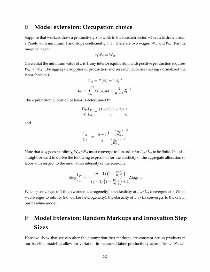
E Model extension: Occupation choice

Suppose that workers draw a productivity x to work in the research sector, where x is drawn from

a Pareto with minimum 1 and slope coefficient η > 1. There are two wages, Wpt and Wrt. For the

marginal agent,

xtWrt = Wpt

Given that the minimum value of x is 1, any interior equilibrium with positive production requires

Wrt ≤ Wpt. The aggregate supplies of production and research labor are (having normalized the

labor force to 1),

Lpt = F (xt) = 1-x−ηt

Lrt =

ˆ ∞

xt

x f (x) dx =η

η − 1x1−η

t .

The equilibrium allocation of labor is determined by

WptLpt

WrtLrt=

(1− α) (1 + τs)

µ

1srt

and

Lpt

Lrt=

η − 1η

1−(

WptWrt

)−η

(WptWrt

)1−η

Note that as η goes to infinity, Wpt/Wrt must converge to 1 in order for Lpt/Lrt to be finite. It is also

straightforward to derive the following expression for the elasticity of the aggregate allocation of

labor with respect to the innovation intensity of the economy:

∆logLpt

Lrt= −

(η − 1)(

1 + Wr LrWp Lp

)(η − 1)

(1 + Wr Lr

Wp Lp

)+ 1

∆logsrt.

When η converges to 1 (high worker heterogeneity), the elasticity of Lpt/Lrt converges to 0. When

η converges to infinity (no worker heterogeneity), the elasticity of Lpt/Lrt converges to the one in

our baseline model.

F Model Extension: Random Markups and Innovation Step

Sizes

Here we show that we can alter the assumption that markups are constant across products in

our baseline model to allow for variation in measured labor productivity across firms. We can

52

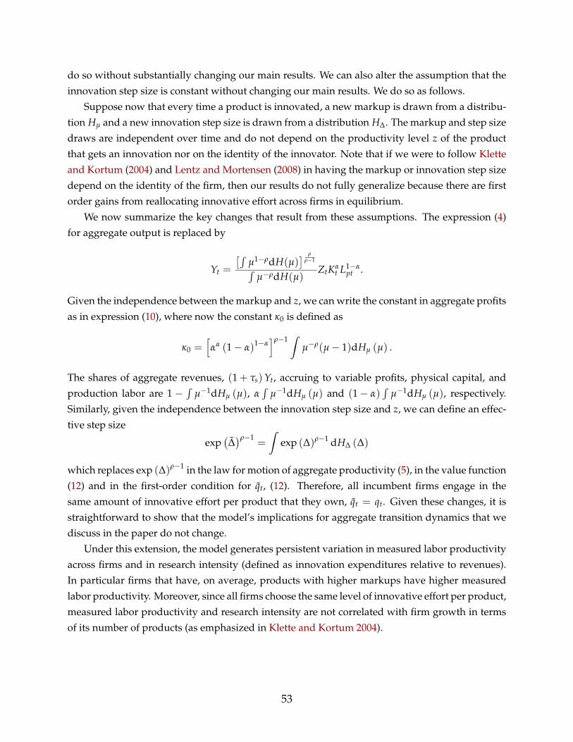
do so without substantially changing our main results. We can also alter the assumption that the

innovation step size is constant without changing our main results. We do so as follows.

Suppose now that every time a product is innovated, a new markup is drawn from a distribu-

tion Hµ and a new innovation step size is drawn from a distribution H∆. The markup and step size

draws are independent over time and do not depend on the productivity level z of the product

that gets an innovation nor on the identity of the innovator. Note that if we were to follow Klette

and Kortum (2004) and Lentz and Mortensen (2008) in having the markup or innovation step size

depend on the identity of the firm, then our results do not fully generalize because there are first

order gains from reallocating innovative effort across firms in equilibrium.

We now summarize the key changes that result from these assumptions. The expression (4)

for aggregate output is replaced by

Yt =

[´µ1−ρdH(µ)

] ρρ−1´

µ−ρdH(µ)ZtKα

t L1−αpt .

Given the independence between the markup and z, we can write the constant in aggregate profits

as in expression (10), where now the constant κ0 is defined as

κ0 =[αα (1− α)1−α

]ρ−1ˆ

µ−ρ(µ− 1)dHµ (µ) .

The shares of aggregate revenues, (1 + τs)Yt, accruing to variable profits, physical capital, and

production labor are 1 −´

µ−1dHµ (µ), α´

µ−1dHµ (µ) and (1− α)´

µ−1dHµ (µ), respectively.

Similarly, given the independence between the innovation step size and z, we can define an effec-

tive step size

exp(∆)ρ−1

=

ˆexp (∆)ρ−1 dH∆ (∆)

which replaces exp (∆)ρ−1 in the law for motion of aggregate productivity (5), in the value function

(12) and in the first-order condition for qt, (12). Therefore, all incumbent firms engage in the

same amount of innovative effort per product that they own, qt = qt. Given these changes, it is

straightforward to show that the model’s implications for aggregate transition dynamics that we

discuss in the paper do not change.

Under this extension, the model generates persistent variation in measured labor productivity

across firms and in research intensity (defined as innovation expenditures relative to revenues).

In particular firms that have, on average, products with higher markups have higher measured

labor productivity. Moreover, since all firms choose the same level of innovative effort per product,

measured labor productivity and research intensity are not correlated with firm growth in terms

of its number of products (as emphasized in Klette and Kortum 2004).

53

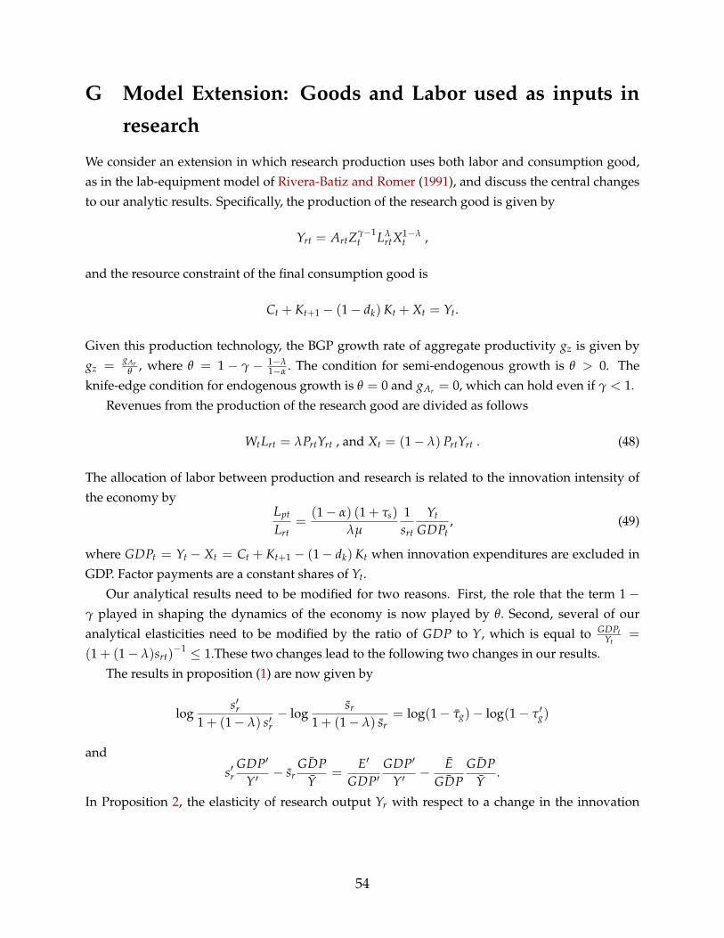
G Model Extension: Goods and Labor used as inputs in

research

We consider an extension in which research production uses both labor and consumption good,

as in the lab-equipment model of Rivera-Batiz and Romer (1991), and discuss the central changes

to our analytic results. Specifically, the production of the research good is given by

Yrt = ArtZγ−1t Lλ

rtX1−λt ,

and the resource constraint of the final consumption good is

Ct + Kt+1 − (1− dk)Kt + Xt = Yt.

Given this production technology, the BGP growth rate of aggregate productivity gz is given by

gz =gAr

θ , where θ = 1 − γ − 1−λ1−α . The condition for semi-endogenous growth is θ > 0. The

knife-edge condition for endogenous growth is θ = 0 and gAr = 0, which can hold even if γ < 1.

Revenues from the production of the research good are divided as follows

WtLrt = λPrtYrt , and Xt = (1− λ) PrtYrt . (48)

The allocation of labor between production and research is related to the innovation intensity of

the economy byLpt

Lrt=

(1− α) (1 + τs)

λµ

1srt

Yt

GDPt, (49)

where GDPt = Yt − Xt = Ct + Kt+1 − (1− dk)Kt when innovation expenditures are excluded in

GDP. Factor payments are a constant shares of Yt.

Our analytical results need to be modified for two reasons. First, the role that the term 1−γ played in shaping the dynamics of the economy is now played by θ. Second, several of our

analytical elasticities need to be modified by the ratio of GDP to Y, which is equal to GDPtYt

=

(1 + (1− λ)srt)−1 ≤ 1.These two changes lead to the following two changes in our results.

The results in proposition (1) are now given by

logs′r

1 + (1− λ) s′r− log

sr

1 + (1− λ) sr= log(1− τg)− log(1− τ′g)

and

s′rGDP′

Y′− sr

¯GDPY

=E′

GDP′GDP′

Y′− E

¯GDP

¯GDPY

.

In Proposition 2, the elasticity of research output Yr with respect to a change in the innovation

54

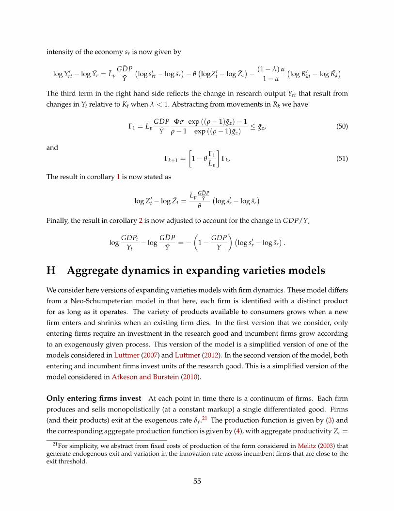
intensity of the economy sr is now given by

log Y′rt − log Yr = Lp¯GDPY

(log s′rt − log sr

)− θ

(logZ′t − log Zt

)− (1− λ) α

1− α

(log R′kt − log Rk

)The third term in the right hand side reflects the change in research output Yrt that result from

changes in Yt relative to Kt when λ < 1. Abstracting from movements in Rk we have

Γ1 = Lp¯GDPY

Φσ

ρ− 1exp ((ρ− 1)gz)− 1

exp ((ρ− 1)gz)≤ gz, (50)

and

Γk+1 =

[1− θ

Γ1

Lp

]Γk, (51)

The result in corollary 1 is now stated as

log Z′t − log Zt =Lp

¯GDPY

θ

(log s′r − log sr

)Finally, the result in corollary 2 is now adjusted to account for the change in GDP/Y,

logGDPt

Yt− log

¯GDPY

= −(

1− GDPY

) (log s′r − log sr

).

H Aggregate dynamics in expanding varieties models

We consider here versions of expanding varieties models with firm dynamics. These model differs

from a Neo-Schumpeterian model in that here, each firm is identified with a distinct product

for as long as it operates. The variety of products available to consumers grows when a new

firm enters and shrinks when an existing firm dies. In the first version that we consider, only

entering firms require an investment in the research good and incumbent firms grow according

to an exogenously given process. This version of the model is a simplified version of one of the

models considered in Luttmer (2007) and Luttmer (2012). In the second version of the model, both

entering and incumbent firms invest units of the research good. This is a simplified version of the

model considered in Atkeson and Burstein (2010).

Only entering firms invest At each point in time there is a continuum of firms. Each firm

produces and sells monopolistically (at a constant markup) a single differentiated good. Firms

(and their products) exit at the exogenous rate δ f .21 The production function is given by (3) and

the corresponding aggregate production function is given by (4), with aggregate productivity Zt =

21For simplicity, we abstract from fixed costs of production of the form considered in Melitz (2003) thatgenerate endogenous exit and variation in the innovation rate across incumbent firms that are close to theexit threshold.

55

[´z exp(z)ρ−1dJt(z)

] 1ρ−1 where the measure of firms

´z dJt(z) can expand or contract depending on

the entry and exit of firms rather than being fixed at 1. Conditional on survival, an incumbent

firm’s productivity z increases by a step size ∆z with a fixed probability q and decreases by −∆z

with probability 1− q. Creating a new firm in period t requires an investment of f units of the

research good. That firm starts production of a new differentiated good in period t + 1 with

productivity zt+1, which grows exogenously at a rate gz = zt+1 − zt. Let Mt denote the measure

of entering firms at time t. The research good is produced with labor according to Yrt = ArtZγt Lrt

and the resource constraint for the research good is f Mt = Yrt. It is convenient to define Yrt =

Yrt

(exp(zt)Zt

)ρ−1, which in a BGP with firm entry is constant at ¯Yrt =

¯Yr.

Under these assumptions, we can write the law of motion of aggregate productivity as

(Zt+1

Zt

)= H(Yrt) =

[H (0)ρ−1 +

Yrt

fexp (gz)

ρ−1] 1

ρ−1

,

where H (0)ρ−1 =(1− δ f

) [qexp (∆z)

ρ−1 + (1− q) exp (−∆z)ρ−1]. In a BGP with positive entry,

the growth rate of aggregate productivity is gz =gAr+(ρ−1)gz

θ , where θ = ρ− 1− γ ≥ 0.

We now compute and bound the elasticity of aggregate productivity growth with respect to the

innovation intensity of the economy. We do so in two steps. In the first, we compute the elasticity

of aggregate productivity growth with respect to normalized research output Yrt. In the second

step, we compute the elasticity of normalized research output Yrt with respect to the innovation

intensity of the economy. By direct calculation, the first elasticity is

H′(Yr)

H(Yr)Yr

∣∣∣∣Yr=

¯rY=

1ρ− 1

(H( ¯Yr)ρ−1 − H (0)ρ−1

H( ¯Yr)ρ−1

)≤ logH( ¯Yr)− logH(0).

Note first that, as before, H( ¯Yr) is calibrated to equal the exponent of the BGP growth rate of

aggregate productivity, exp (gz). The term H (0) is no longer equal to one as in our baseline Neo-

Schumpeterian model, but instead it is determined by the exit rate of incumbent firms together

with the growth rate of those incumbents that survive. One can show that in this model, to ensure

a stationary firm size distribution with positive firm entry, it is necessary to have H (0) < 1.

Moreover, in this model the term that determines the elasticity above, H( ¯Yr)ρ−1−H(0)ρ−1

H( ¯Yr)ρ−1 , is equal to

the share of employment by entering firms in the BGP.

To compute the elasticity of normalized research output with respect to the innovation inten-

sity of the economy, we use the fact that Yrt = Artexp (zt)ρ−1 Z−θ

t Lrt and that equation (17) in our

baseline model still applies.

Using these results, we can derive the analog of equation (28) in Proposition 2. In an economy

that is initially on a BGP with positive firm-entry, an unanticipated, permanent change in inno-

vation policies (i.e. subsidy to firm entry) that induces a new path for the innovation intensity of

the economy given by {s′rt}∞t=0, the new path for aggregate productivity {Z′t}

∞t=1 to a first-order

56

approximation is given by

log(

Z′t+1

Z′t

)− gz =

(exp (gz)

ρ−1 − H (0)ρ−1

exp (gz)ρ−1

)1

ρ− 1[Lp(log s′rt − log sr

)− θ

(logZ′t − logZt

)].

(52)

Both entering firms and incumbent firms invest We now extend the previous model and

assume that incumbent firms can invest resources to increase the productivity of the product they

own. A firm owning a product with productivity z that invests exp(

zzt

)ρ−1c (q− ql) units of the

research good in the current period t has a probability q ≥ ql that its productivity z increases by

a step size ∆z and a probability 1− q that productivity decreases by ∆z, where c (.) is increasing

and convex with c (0) = 0. The assumption that the cost of innovation falls with the productivity

of entrants ensures that incumbent firms innovate in the long run.

Under these assumptions it is straightforward to show that all continuing firms choose the

same level of q, independent of their productivity z (given our assumption that the cost scales

up with exp (z)ρ−1). In an equilibrium with positive entry, qt is determined from the following

condition: (1− τg

)c′ (qt) =

(1− τe) f(1− δ f

)exp (gz)

ρ−1

[exp (∆z)

ρ−1 − exp (−∆z)ρ−1]

. (53)

where qt = qt − ql . The law of motion for aggregate productivity is(Zt+1

Zt

)= H

(Mt, qt

)=[

H (0, 0)ρ−1 + exp (gz)ρ−1 Mt +

(1− δ f

)qt

[exp (∆z)

ρ−1 − exp (−∆z)ρ−1]] 1

ρ−1

(54)

where Mt =(exp(zt)

Zt

)ρ−1Mt, and H (0, 0)ρ−1 =

(1− δ f

) [qlexp (∆z)

ρ−1 + (1− ql) exp (−∆z)ρ−1]

is the growth rate of aggregate productivity when Mt = 0 and qt = ql (that is, when aggregate

innovation expenditure is zero). Note that this transition law for aggregate productivity is a func-

tion of both Mt and qt and not simply a function of output of the research good Yrt as in the

previous model. As we show below, we will be able to derive a meaningful elasticity of aggregate

productivity with respect to the innovation intensity of the economy starting from an initial BGP

with uniform innovation policies as we did in our baseline Klette-Kortum model. The resource

constraint for the research good is

Yrt = Artexp (zt)ρ−1 Z−θ

t Lrt = Mt f + c (qt) . (55)

We now compute the elasticity of aggregate productivity growth with respect to normalized

research output starting in an initial equilibrium with positive firm entry and uniform innovation

57

subsidies (i.e. τg = τe). We first have

dH(

M, q)

dYr=

[∂H(

M, q)

∂MdMdYr

+∂H(

M, q)

∂qdqdYr

]=

1ρ− 1

exp (gz)ρ−1

f H(

¯M, ¯q)ρ−2

where we used equations (53) and (55), which implies

dH(

M, q)

H(M,q)

dYrYr

=1

ρ− 1

¯Yrexp (gz)ρ−1

f H(

¯M, ¯q)ρ−1 .

Using equations (54), (53) and (55) in a BGP with uniform innovation policies and positive firm

entry, we can re-write this elasticity as

dH(

M, q)

H(M,q)

dYrYr

=Φ

ρ− 1

H(

¯M, ¯q)ρ−1

− H (0, 0)ρ−1

H(

¯M, ¯q)ρ−1 ,

with

Φ =¯Yr

¯Yr + c′ ( ¯q) ¯q− c ( ¯q)< 1

The last inequality follows from the convexity of c (·) together with the assumption that c (0) = 0.

Note that in our baseline Klette-Kortum, Φ can also be written in this way.

We can obtain the elasticity of normalized research output with respect to the innovation in-

tensity of the economy following the same steps as above. We obtain dynamics for aggregate

productivity in response to policy-induced (uniform or non-uniform) changes in the innovation

intensity of the economy given by

log(

Z′t+1

Z′t

)− gz =

(exp (gz)

ρ−1 − H (0, 0)ρ−1

exp (gz)ρ−1

)Φ

ρ− 1[Lp(log s′rt − log sr

)− θ

(logZ′t − logZt

)].

In this model, assigning a value to H (0, 0) would require knowing what the exit rate is and what

the growth rate of productivity for incumbent firms is if these firms set their innovation spending

to zero.

58