Navigating the US truckload capacity cycle: Where are ... · development and consulting roles at Adjoined Consulting (now Capgemini), Agile Software Corp. (now Oracle), Electron Economy

© HENRY STEWART PUBLICATIONS 2516-1814 JOURNAL OF SUPPLY CHAIN MANAGEMENT, LOGISTICS AND PROCUREMENT VOL. 1, NO. 1, 1–18 SUMMER 2018 1

Navigating the US truckload capacity cycle: Where are freight rates headed and why?Received (in revised form): 4th May, 2018

CHRIS PICKETTis Chief Strategy Officer at Coyote Logistics, a leading provider of non-asset based third-party logistics (3PL) solutions across North America and Europe. Chris is responsible for helping the Coyote leadership team develop, evolve, and execute an enterprise growth strategy geared toward leveraging Coyote’s unique operating advantages across an increasingly dynamic global market and competitive landscape. He is also responsible for all activities related to North American Sales, Marketing, Operations, Supply Chain Engineering and Pricing Strategy — ensuring that all are aligned to identify, implement and innovate capacity, process and technology solutions for shippers across the global Coyote network. Before joining Coyote in 2006, Chris served in various strategy development and consulting roles at Adjoined Consulting (now Capgemini), Agile Software Corp. (now Oracle), Electron Economy (now Viewlocity) and Andersen Consulting (now Accenture). Throughout his career, Chris has architected, implemented, and managed diverse supply chain (SC) management and customer service-related projects for a variety of global market leaders in the food and beverage, pharmaceutical, telecommunications, and consumer technology sectors. He earned a B.S. in Industrial & Systems Engineering from Virginia Tech, an M.Eng. in Logistics from MIT, and an MBA from Georgia Tech. Founded in 2006 and headquartered in Chicago, Coyote Logistics, LLC, a UPS company, is a leading 3PL service provider in North America and Europe. Coyote provides truckload, less-than-truckload, intermodal and cross-border brokerage and transportation management services to more than 14,000 shippers utilising a network of 50,000 carriers. Coyote became a UPS company in August 2015, adding UPS asset utilisation, air freight, ocean freight, customs brokerage and much more to its portfolio of services. Coyote is a proud philanthropic supporter of St. Jude Children’s Research Hospital, for which has raised more than $2.3m in seven years. For more information about Coyote, please visit www.coyote.com.

AbstractThe US truckload transportation market, like many markets, can be characterised as an ongoing rebalancing between supply and demand — or in this case, the number of trucks (and drivers) to haul goods and the demand for those trucks to meet current market demand. This creates a cycle that swings from relative capacity shortage, where there is more demand relative to supply which drives market rates higher, to relative capacity surplus, where there is more supply available relative to demand which drives rates lower. The term ‘relative’ is an important one as the simultaneous rate of change on both sides of the marketplace ultimately drives market rate activity. But as this article will go on to describe, the simultaneous rates of change in supply and demand are rarely in a state of relative equilibrium. It is this dynamic that creates a recurring pricing cycle observed to display at least some level of consistency and can therefore be used to predict the future — but only if you understand the past and the present. In other words, the US truckload market operates as a machine with certain mechanical properties that tend to produce similar outputs given similar inputs. The real world is governed by economic and geopolitical uncertainty, shifting technology and regulatory landscapes, and human psychology that often drives irrational behaviour, so those mechanical properties and input signals can be exceedingly difficult to separate from the noise. However, with enough historical transaction data, market visibility, and insight, I propose that it can be done; the past can be used to predict the future with at least some level of directional certainty, so long as the fundamental structure of the marketplace remains intact.

Keywordstransportation, logistics, freight rates, trucking, procurement, supply chain economics

Chris Pickett, Chief Strategy OfficerCoyote Logistics, a UPS Company, 2545 W Diversey Ave, 3rd Floor, Chicago, IL 60647, USA

Tel: +1 847-235-8241; E-mail: [email protected]

Chris Pickett

Pickett

2 © HENRY STEWART PUBLICATIONS 2516-1814 JOURNAL OF SUPPLY CHAIN MANAGEMENT, LOGISTICS AND PROCUREMENT VOL. 1, NO. 1, 1–18 SUMMER 2018

MARKET STRUCTUREThe $800bn1 trucking industry in the US is large, growing and extremely fragmented. It is comprised of hundreds of thousands of markets participants making respective buy and sell decisions based on individual economic self-interest. All over different planning horizons, operating strategies and financial constraints. All with varying levels of market information at any given time. And all executing transactions under varying terms in a market system that is defined by uncertainty and delayed feedback loops, which ultimately drives exaggerated responses to market signals that set up repeated cycles of supply overshoot and market rate collapse and recovery.

The demand side of this market is comprised of hundreds of thousands of manufacturers, wholesalers, importers, exporters and retailers that are constantly making choices as to best to serve their end markets. In other words, where to ship, what to ship, and in what quantities or in what configurations to ship their respective products — whether it be raw materials, intermediate goods or final products ready for end user consumption. They make these decisions based on a wide variety of objectives, input data and assumptions — one of which is the method of transportation between SC nodes. In general, shippers make production decisions in response to their own end market demand patterns and the general economics of their respective businesses. They choose what to make and in what quantities or configura-tions given whatever operational or SC constraints may exist over whatever planning horizon they are executing against. These choices generate volume demand for transportation in general, and truckload transportation more

specifically. The balance of available supply to meet this demand is what determines market pricing.

The supply side of the market is just as large and fragmented with barriers to entry and exit that are just as low. According to the American Trucking Association,2 there were over 580,000 for-hire common carriers registered with the Federal Motor Carrier Safety Administration in 2015, and another 747,781 private carriers. Over 97 per cent of those carriers reported operating fewer than 20 trucks with almost 91 per cent operating six or fewer. And while there are several large national carriers with tractor fleets in the 10,000–20,000 range, the top 15 carriers account for less than 12 per cent of total for-hire market revenue.3 So, this is a supply base that in many ways is dominated by the long tail of hundreds of thousands of small and medium-sized trucking companies and individual owner-operators. But the decision criteria that typically drives fleet decisions (ie to expand, shrink or remain neutral) are likely the same across all segments. If capital is available and the expected return on investment is attractive, enter the market or grow the fleet. If the expected return is not attractive, remain neutral. And if current and expected future operating profits are especially unattractive, shrink or exit the market altogether. This repeated pattern of behaviour is what ultimately drives the long-term capacity cycle, which we observe to be the most pervasive driver of long-term market pricing behaviour.

THE CAPACITY CYCLEIn a very large, extremely fragmented market with very low barriers to entry and exit, and no one market participant large enough to dictate market pricing

NavigatiNg the US trUckload caPacity cycle


with any level of consistency, market pricing is left to float based on the balance of supply versus demand that is in a state of perpetual flux. Therefore, equilibrium pricing is only temporary and subject to significant swings driven by a variety of ever-shifting market dynamics like economic activity, shifting seasonal demand patterns, regulatory changes and even in some cases, the weather. When conditions are attractive, truckers order more trucks thus increasing market capacity. Eventually those trucks come to market at some future date (based on build cycles, order backlogs, used equipment availability, etc.). And as is often the case, the future has little resemblance to the point in time in which those original capacity decisions were made. Eventually, supply exceeds demand and market rates decline on a relative basis. Market rates will continue to decline until equilibrium levels are reached and enough excess capacity has been forced from the marketplace. As market rates recover, current demand begins to exceed current supply, and the next period of inflationary rate condi-tions is initiated, thus triggering the next capacity cycle. It all sounds very straight-forward and logical when described in this way, however things tend to get more than a little messy in the real world, which can make the natural order of things exceedingly difficult to perceive.

REAL-WORLD COMPLEXITY: THREE PRIMARY CYCLES OPERATING SIMULTANEOUSLYAside from the uncertainty and noise generated in a marketplace in which often irrational human beings interact within an increasingly dynamic and volatile US economy, there are also two other major cycles running alongside

the market capacity cycle that we must reconcile. They are the two that market participants are most familiar with and easier to observe and understand because they tend to be calendar-driven and right in front of us most of the time.

The seasonal demand cycleThe first cycle applies to the seasonal demand dislocations that occur over the year with at least some level of regularity. The average year-round levels of specific products or commodities surge over a relatively short period of time, generally weeks or in some cases months, in response to planned production or demand windows. Examples of this include produce seasons in the southeast, Texas and California where growing seasons and conditions dictate product availability. As a result, this generates a high premium for speed to market to maximise shelf lives and ultimately end consumer sales. All else equal, this drives inflationary rate conditions across the outbound regions from which various types of produce are harvested that last the duration of the growing season as shippers must pay whatever the market demands to ensure speed to market, which often has ripple effects across the rest of the country. Historically, south and southeastern US produce season effects are seen as early as April and as late as July though always subject to weather and growing conditions.

Other examples include Christmas trees and retail peak season. Christmas trees generally ship out of the Pacific Northwest and Carolinas in November and December. Imports to support peak retail activity around the holidays tend to surge into West Coast ports (and increas-ingly Gulf and East Coasts with the expansion of the Panama Canal in 2016)

Pickett


in September and October. In turn, both brick-and-mortar and e-commerce retailers surge from the middle of November through the middle of January to support both outbound gift giving and inbound returns. Trucks migrate to service these markets and capitalise on the demand dislocation for as long as it exists, as rational market behaviour would dictate, then disperse across other market geographies accordingly. Trucks and truck drivers, in many ways, are the ultimate form of mobile production, which means that demand dislocations can usually be absorbed by the market very efficiently but also that they do not last forever as the relative balance of supply versus demand eventually adjusts.

A corollary to known seasonal demand dislocations worth noting here lies in unexpected catastrophic weather events that create relatively short-term but often profound dislocations in both demand and supply — the most recent example being Hurricanes Harvey and Irma that battered the southern and eastern US in rapid succession in August and September 2017 causing unprecedented flooding across the entire Houston, TX metropolitan area. While there was a sudden unplanned need for rescue and relief supplies in the affected regions coupled with major disruptions in the transportation infra-structure and network required to support the recovery that drove infla-tionary inbound TL rates, that was not the only market force in play. In a major weather event like this, there is also outbound supply dislocation to consider. If a shipper normally fulfills their southwest demand from a distri-bution centre in Houston, and if that facility suddenly finds itself under 4 feet of standing water, they will likely be looking for alternate sources of supply.

Therefore, as otherwise consistent freight flows are disrupted, they will likely be procuring unplanned trans-portation capacity over irregular lanes at current spot market rates — at the same time as the rest of market. This broader network disruption acts as an additional inflationary force thereby amplifying the market impact of weather events that fall into this extreme category.

The annual procurement cycleThe second cycle is tied to the schedule by which higher-volume shippers go out to market to set fixed contract rates for the next fiscal period. Just as many organisations find value in setting stable rates for fixed supply of many of the raw materials that go into their products or packaging, many treat truckload transportation in the same way — as a commodity that can sometimes exhibit volatile price behaviour and supply risk they would rather not bear given other financial and operational objectives and constraints. So, they engage the marketplace based on their respective procurement strategies and seek to set or reset contract rates for the lanes in their forecasted network to cover the number of shipments they expect to ship over the contract period subject to a variety of factors and considerations. While shippers can be out in the market throughout the year, we observe that most of the largest volume shippers in the US tend to go out to bid in the fourth quarter to lock in new contract rates that are then activated in the following first or second quarter. Typically, agree-ments are expected to be honoured over the subsequent 12-month period. We find that, across the market as a whole, contract rates tend to reset in late first quarter or early second quarter and then



reset again the following year around the same time.

By itself, this is a perfectly logical way to contract so long as there is consistency over the years. And this consistency should act as a long-term stabilising force as a whole, thus dampening general rate volatility across both the spot and contract portions of the marketplace. But the shifting dynamics created through the simultaneous activity of the annual procurement cycle, seasonal demand cycle and capacity cycle can often generate a tremendous amount of noise driven by conflicting economic indicators, uncertain and ever-changing forecasts, and general posturing from both sides of the marketplace as partici-pants advocate for both higher and lower market prices. With both the seasonal demand and annual procurement cycles as well entrenched in our collective psyches as they are, the presence of an underlying capacity cycle that dominates both over the long-term does not appear to be well understood. That said, with the appropriate data set, time horizon, and methodology, we believe to have identified observable and quantifiable evidence of such a cycle.

The elusive capacity cycle‘What is going on in the market?’ ‘How much worse is it going to get?’ ‘What happened to my freight budget?’ ‘How do I become a shipper of choice?’ These are all questions that you hear a lot more in the midst of the inflationary leg of a capacity cycle like the one we are in right now. Freight budgets were set and contract rates were negotiated during a period of relative market deflation or even equilibrium, and suddenly all of that is out the window. Contracts are breaking down as carriers refuse load

tenders at those contract rates to gain relative exposure to an increasingly more attractive spot market. More freight is falling through the routing guide to move at relatively higher spot or backup rates, and both budget variance and service levels are suffering as a result. All of this because shippers and carriers forecasted a future that failed to materialise, and they must now adapt to the future that did. Less abstractly, they expected a relatively benign forward rate environment after a prolonged period of deflation, where supply would be in relative equilibrium to demand. Then they contracted, set budgets, made fleet decisions as such — and then rate inflation happened.

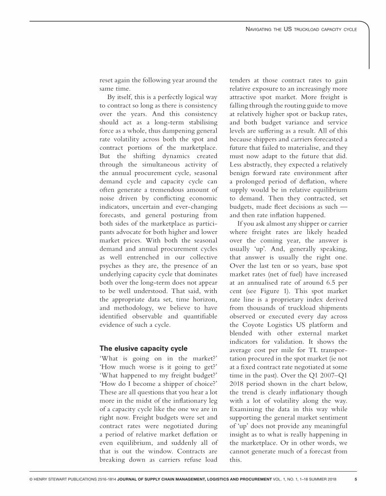
If you ask almost any shipper or carrier where freight rates are likely headed over the coming year, the answer is usually ‘up’. And, generally speaking, that answer is usually the right one. Over the last ten or so years, base spot market rates (net of fuel) have increased at an annualised rate of around 6.5 per cent (see Figure 1). This spot market rate line is a proprietary index derived from thousands of truckload shipments observed or executed every day across the Coyote Logistics US platform and blended with other external market indicators for validation. It shows the average cost per mile for TL transpor-tation procured in the spot market (ie not at a fixed contract rate negotiated at some time in the past). Over the Q1 2007–Q1 2018 period shown in the chart below, the trend is clearly inflationary though with a lot of volatility along the way. Examining the data in this way while supporting the general market sentiment of ‘up’ does not provide any meaningful insight as to what is really happening in the marketplace. Or in other words, we cannot generate much of a forecast from this.

Pickett


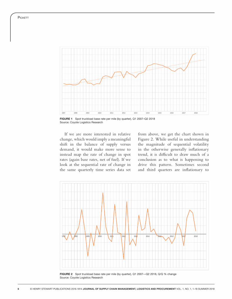
If we are more interested in relative change, which would imply a meaningful shift in the balance of supply versus demand, it would make more sense to instead map the rate of change in spot rates (again base rates, net of fuel). If we look at the sequential rate of change in the same quarterly time series data set

from above, we get the chart shown in Figure 2. While useful in understanding the magnitude of sequential volatility in the otherwise generally inflationary trend, it is difficult to draw much of a conclusion as to what is happening to drive this pattern. Sometimes second and third quarters are inflationary to

FIGURE 1 Spot truckload base rate per mile (by quarter), Q1 2007–Q2 2018Source: Coyote Logistics Research

FIGURE 2 Spot truckload base rate per mile (by quarter), Q1 2007––Q2 2018, Q/Q % changeSource: Coyote Logistics Research



first quarters due to seasonal demand patterns, while sometimes they are not — like in 2009 and 2015. First quarters are often deflationary to fourth quarters as peak retail demand surges abate, but again sometimes they are not — like in 2014 and 2018. So, while maybe debunking a few market myths like ‘it’s always soft (ie deflationary) in January and February’ or ‘it is always tight (ie inflationary) in the southeast in June and July’, it is difficult to discern anything especially meaningful by inspecting rate data in this manner. In many ways, it would appear that rates move somewhat randomly according to the short-term ebbs and flows of the marketplace.

But what if we try to neutralise the effects of known seasonality, so that we are always comparing one produce season or peak season to another? If we take the same quarterly time series data and instead of mapping the sequential change from the subsequent quarter, we look at the annual change from the same quarter in the subsequent year, would

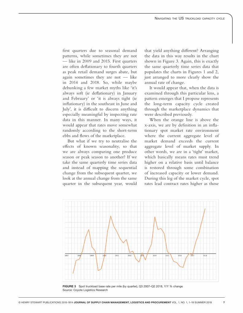
that yield anything different? Arranging the data in this way results in the chart shown in Figure 3. Again, this is exactly the same quarterly time series data that populates the charts in Figures 1 and 2, just arranged to more clearly show the annual rate of change.

It would appear that, when the data is examined through this particular lens, a pattern emerges that I propose represents the long-term capacity cycle created through the marketplace dynamics that were described previously.

When the orange line is above the x-axis, we are by definition in an infla-tionary spot market rate environment where the current aggregate level of market demand exceeds the current aggregate level of market supply. In other words, we are in a ‘tight’ market, which basically means rates must trend higher on a relative basis until balance is restored through some combination of increased capacity or lower demand. During this leg of the market cycle, spot rates lead contract rates higher as those

FIGURE 3 Spot truckload base rate per mile (by quarter), Q3 2007–Q2 2018, Y/Y % changeSource: Coyote Logistics Research

Pickett


rates reset to current market conditions according to the annual procurement cycle. Eventually rates remain high enough for long enough, relative to the primary carrier input costs of labour and fuel, that incremental capacity is brought to market in response. Eventually, as irrational humans making long-term financial decisions in a rapidly shifting marketplace often do, we get greedy and overshoot. Too much incremental capacity eventually enters the market relative to market demand and the supply-demand balance reverses. The rate of annual market inflation peaks then heads towards zero (or relative equilibrium), then into the deflationary leg of the cycle where rates drop until sufficient surplus capacity, relative to demand, is forced to exit the market. The rate of decline is halted before reversing on the journey back to equilibrium and into the infla-tionary leg of the next cycle.

As we continue, most of the remaining charts will be configured by looking at quarterly averages on a year-over-year basis thus showing true annualised inflation or deflation void of the seasonal noise. When we are above the x-axis, we are in inflation land where rates (in this case) are higher than they were in the same quarter last year. And when we are below, we reside in deflation land where rates are relatively lower than last year. As you can see, consistent with the long-term inflationary time series chart that we started with, our stays in inflation land tend to be much longer in duration and peak much higher before inflecting than our time below the x-axis in deflation land.

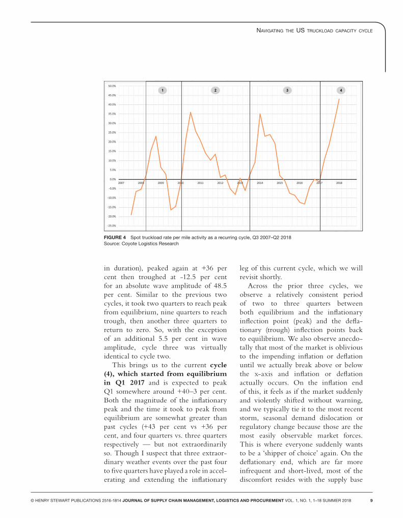
While the sinusoidal nature of the curve appears relatively consistent in some ways, both the periods and amplitudes show some variation. For the purposes of this discussion, I propose that a complete

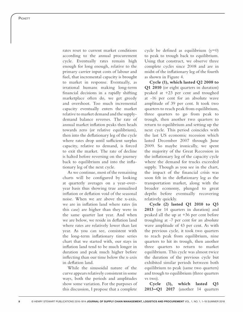
cycle be defined as equilibrium (y=0) to peak to trough back to equilibrium. Using that construct, we observe three complete cycles since 2008 and are in midst of the inflationary leg of the fourth as shown in Figure 4.

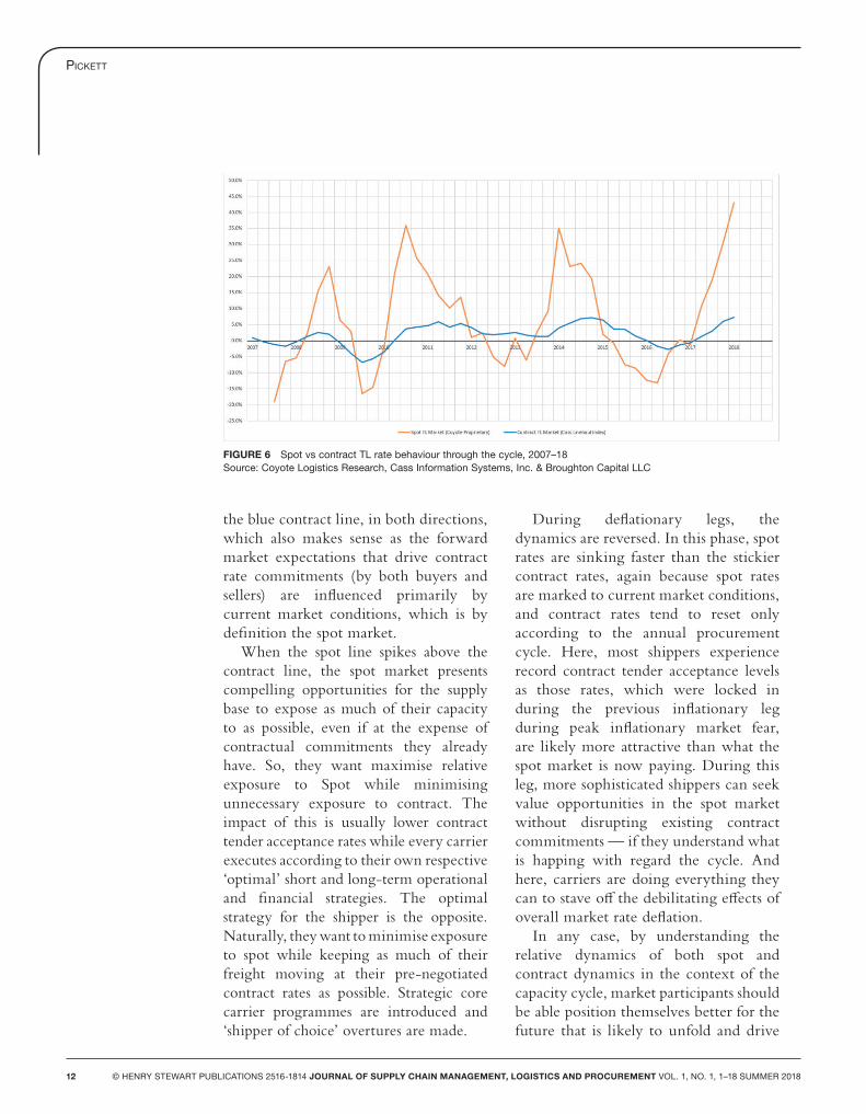
Cycle (1), which lasted Q2 2008 to Q1 2010 (or eight quarters in duration) peaked at +23 per cent and troughed at -16 per cent for an absolute wave amplitude of 39 per cent. It took two quarters to reach peak from equilibrium, three quarters to go from peak to trough, then another two quarters to return to equilibrium and setting up the next cycle. This period coincides with the last US economic recession which lasted December 2007 through June 2009. So maybe ironically, we spent the majority of the Great Recession in the inflationary leg of the capacity cycle where the demand for trucks exceeded supply. Though as you see in the chart, the impact of the financial crisis was soon felt in the deflationary leg as the transportation market, along with the broader economy, plunged to great depths before eventually recovering relatively quickly.

Cycle (2) lasted Q1 2010 to Q3 2013 (or 14 quarters in duration) and peaked all the up at +36 per cent before troughing at -7 per cent for an absolute wave amplitude of 43 per cent. As with the previous cycle, it took two quarters to reach peak from equilibrium, nine quarters to hit its trough, then another three quarters to return to market equilibrium. This cycle was almost twice the duration of the previous cycle but exhibited similar periods between both equilibrium to peak (same two quarters) and trough to equilibrium (three quarters vs two).

Cycle (3), which lasted Q3 2013–Q1 2017 (another 14 quarters



in duration), peaked again at +36 per cent then troughed at -12.5 per cent for an absolute wave amplitude of 48.5 per cent. Similar to the previous two cycles, it took two quarters to reach peak from equilibrium, nine quarters to reach trough, then another three quarters to return to zero. So, with the exception of an additional 5.5 per cent in wave amplitude, cycle three was virtually identical to cycle two.

This brings us to the current cycle (4), which started from equilibrium in Q1 2017 and is expected to peak Q1 somewhere around +40–3 per cent. Both the magnitude of the inflationary peak and the time it took to peak from equilibrium are somewhat greater than past cycles (+43 per cent vs +36 per cent, and four quarters vs. three quarters respectively — but not extraordinarily so. Though I suspect that three extraor-dinary weather events over the past four to five quarters have played a role in accel-erating and extending the inflationary

leg of this current cycle, which we will revisit shortly.

Across the prior three cycles, we observe a relatively consistent period of two to three quarters between both equilibrium and the inflationary inflection point (peak) and the defla-tionary (trough) inflection points back to equilibrium. We also observe anecdo-tally that most of the market is oblivious to the impending inflation or deflation until we actually break above or below the x-axis and inflation or deflation actually occurs. On the inflation end of this, it feels as if the market suddenly and violently shifted without warning, and we typically tie it to the most recent storm, seasonal demand dislocation or regulatory change because those are the most easily observable market forces. This is where everyone suddenly wants to be a ‘shipper of choice’ again. On the deflationary end, which are far more infrequent and short-lived, most of the discomfort resides with the supply base

FIGURE 4 Spot truckload rate per mile activity as a recurring cycle, Q3 2007–Q2 2018Source: Coyote Logistics Research

Pickett


as rates must drift lower to clear surplus capacity and painful choices are often required. Here in deflation land, ‘carrier of choice’ takes the place of ‘shipper of choice’ in the industry lexicon.

But these market shifts that often feel sudden and out of the blue are telegraphed several quarters in advance as inflection points are reached and rates of change begin their journey towards equilibrium. These are slow moving cycles as it takes time for a market this large and fragmented to reach its collective pain threshold — either when increasing supply levels no longer support higher and higher market pricing, or when diminished supply levels no longer allow rates to sink any lower.

With these historically consistent mechanical properties in mind, given where we are in Q1 2018, one would expect the spot market to remain in an inflationary state through the end of the year before reaching equilibrium and potential deflation by early 2019 as the market historically just does not move

faster than that. But with that said, we return to the topic of extraordinary weather.

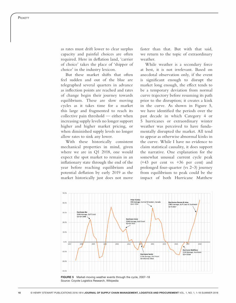
While weather is a secondary force at best, it is not irrelevant. Based on anecdotal observation only, if the event is significant enough to disrupt the market long enough, the effect tends to be a temporary deviation from normal curve trajectory before resuming its path prior to the disruption; it creates a kink in the curve. As shown in Figure 5, we have identified the periods over the past decade in which Category 4 or 5 hurricanes or extraordinary winter weather was perceived to have funda-mentally disrupted the market. All tend to appear as otherwise abnormal kinks in the curve. While I have no evidence to claim statistical causality, it does support the narrative. One explanation for the somewhat unusual current cycle peak (+43 per cent vs +36 per cent) and prolonged four-quarter (vs 2–3) journey from equilibrium to peak could be the impact of both Hurricane Matthew

FIGURE 5 Market-moving weather events through the cycle, 2007–18Source: Coyote Logistics Research, Wikipedia



driving an accelerated recovery from the prior trough and the unprecedented back-to-back Category 4 or 5 Hurricanes Harvey and Irma hitting in the back half of Q3 2017. So, any forward-looking base cycle forecast will be contingent upon extraordinary weather events like those listed below and where in the cycle they occur.

It is also worth noting the apparent increase in the relative occurrence of market-moving weather events in recent years. While 11 years of market pricing and storm data is hardly enough of a time horizon to read too far into, the reality is that we observed only two such events over the first five years (2007–12) of this study and five over the subsequent and most recent five years (2013–17). Should this phenomenon of increased frequency of major market-moving weather events continue, it would be reasonable to expect more frequent kinks in the capacity curve going forward — the net impact being a function of both the magnitude and duration of the event and where we are in the cycle when it occurs, the riskiest periods clearly being cycle peaks like we experienced with Hurricanes Ike in 2008, the 2014 Polar Vortex and Hurricanes Harvey and Irma in 2017.

THE CYCLE WITHIN THE CYCLE: CONTRACT VS SPOT RATESUp to this point, the capacity cycle has been defined in the context of spot market rate dynamics only as that paints the clearest picture of the current balance of supply vs demand across the market-place. But as also discussed, spot rates tend to lead contract rates, and most shippers and carriers tend to be exposed to both markets, though to different degrees based on their respective businesses, operating

strategies, constraints and forward-looking expectations. Their choices over the course of the cycle are shaped by how they positioned themselves going into either an inflationary or deflationary leg, and how the current market conforms to the expectations they had going in. Our proxy of choice for the contract market is the Cass Linehaul Index,4 which is published monthly by Cass Information Systems in conjunction with Broughton Capital, LLC. The Cass index show relative change in TL base rates across the $25bn in annual freight spend that Cass manages on behalf of their customers. In focusing on the Cass index, our working assumption is that the same high-volume shippers that outsource their freight payables to Cass to manage are the same types of shippers with sufficient volume to support an annual procurement exercise to contract all or some portion of their TL spend. While it is assumed that the Cass data includes all freight payables regardless of whether the shipment moved at a contract or spot rate, we assume contract-rated shipments to represent the majority.

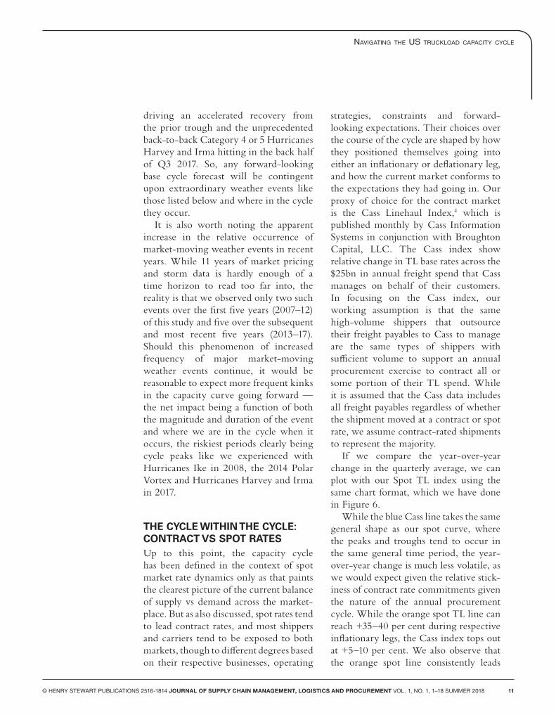
If we compare the year-over-year change in the quarterly average, we can plot with our Spot TL index using the same chart format, which we have done in Figure 6.

While the blue Cass line takes the same general shape as our spot curve, where the peaks and troughs tend to occur in the same general time period, the year-over-year change is much less volatile, as we would expect given the relative stick-iness of contract rate commitments given the nature of the annual procurement cycle. While the orange spot TL line can reach +35–40 per cent during respective inflationary legs, the Cass index tops out at +5–10 per cent. We also observe that the orange spot line consistently leads

Pickett


the blue contract line, in both directions, which also makes sense as the forward market expectations that drive contract rate commitments (by both buyers and sellers) are influenced primarily by current market conditions, which is by definition the spot market.

When the spot line spikes above the contract line, the spot market presents compelling opportunities for the supply base to expose as much of their capacity to as possible, even if at the expense of contractual commitments they already have. So, they want maximise relative exposure to Spot while minimising unnecessary exposure to contract. The impact of this is usually lower contract tender acceptance rates while every carrier executes according to their own respective ‘optimal’ short and long-term operational and financial strategies. The optimal strategy for the shipper is the opposite. Naturally, they want to minimise exposure to spot while keeping as much of their freight moving at their pre-negotiated contract rates as possible. Strategic core carrier programmes are introduced and ‘shipper of choice’ overtures are made.

During deflationary legs, the dynamics are reversed. In this phase, spot rates are sinking faster than the stickier contract rates, again because spot rates are marked to current market conditions, and contract rates tend to reset only according to the annual procurement cycle. Here, most shippers experience record contract tender acceptance levels as those rates, which were locked in during the previous inflationary leg during peak inflationary market fear, are likely more attractive than what the spot market is now paying. During this leg, more sophisticated shippers can seek value opportunities in the spot market without disrupting existing contract commitments — if they understand what is happing with regard the cycle. And here, carriers are doing everything they can to stave off the debilitating effects of overall market rate deflation.

In any case, by understanding the relative dynamics of both spot and contract dynamics in the context of the capacity cycle, market participants should be able position themselves better for the future that is likely to unfold and drive

FIGURE 6 Spot vs contract TL rate behaviour through the cycle, 2007–18Source: Coyote Logistics Research, Cass Information Systems, Inc. & Broughton Capital LLC



better decision that results in stronger outcomes for their respective organisa-tions. At the very least, they could set a more realistic freight budget or reasoned capacity management programme.

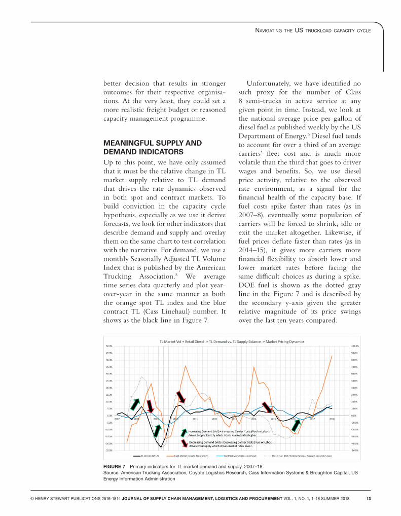
MEANINGFUL SUPPLY AND DEMAND INDICATORSUp to this point, we have only assumed that it must be the relative change in TL market supply relative to TL demand that drives the rate dynamics observed in both spot and contract markets. To build conviction in the capacity cycle hypothesis, especially as we use it derive forecasts, we look for other indicators that describe demand and supply and overlay them on the same chart to test correlation with the narrative. For demand, we use a monthly Seasonally Adjusted TL Volume Index that is published by the American Trucking Association.5 We average time series data quarterly and plot year-over-year in the same manner as both the orange spot TL index and the blue contract TL (Cass Linehaul) number. It shows as the black line in Figure 7.

Unfortunately, we have identified no such proxy for the number of Class 8 semi-trucks in active service at any given point in time. Instead, we look at the national average price per gallon of diesel fuel as published weekly by the US Department of Energy.6 Diesel fuel tends to account for over a third of an average carriers’ fleet cost and is much more volatile than the third that goes to driver wages and benefits. So, we use diesel price activity, relative to the observed rate environment, as a signal for the financial health of the capacity base. If fuel costs spike faster than rates (as in 2007–8), eventually some population of carriers will be forced to shrink, idle or exit the market altogether. Likewise, if fuel prices deflate faster than rates (as in 2014–15), it gives more carriers more financial flexibility to absorb lower and lower market rates before facing the same difficult choices as during a spike. DOE fuel is shown as the dotted gray line in the Figure 7 and is described by the secondary y-axis given the greater relative magnitude of its price swings over the last ten years compared.

FIGURE 7 Primary indicators for TL market demand and supply, 2007–18Source: American Trucking Association, Coyote Logistics Research, Cass Information Systems & Broughton Capital, US Energy Information Administration

Pickett


When overlaying our spot and contract rate curves with our black demand indicator and our dotted gray implied supply indicator, we do observe at least some level of coincidental, if not always leading, behaviour. When demand and fuel are accelerating simul-taneously (our green-outlined arrows above), or demand is increasing while supply is under financial pressure and possibly decreasing, conditions are ripe to support an inflationary TL rate environment. When both are simulta-neously decreasing, it is implied that demand is diminishing at a faster rate than supply, thereby supporting a relatively deflationary rate environment.

While I make no claim of statistical causality with either of these indicators, they have been useful in supporting or contradicting the drivers behind the observed activity of our spot and contract rate indices. For example, both can be leading indicators to future inflection points or can indicate how much higher or lower an inflationary or deflationary leg is likely to run or how long it is likely to last.

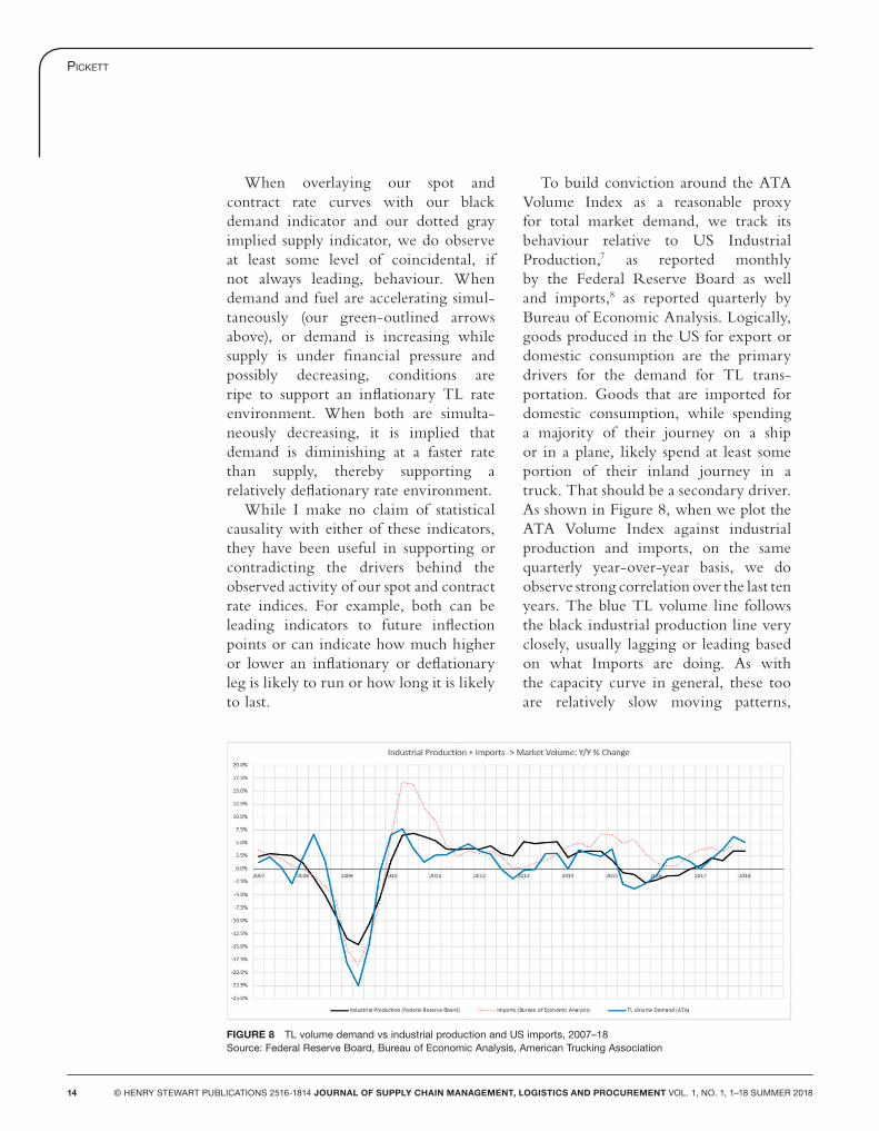
To build conviction around the ATA Volume Index as a reasonable proxy for total market demand, we track its behaviour relative to US Industrial Production,7 as reported monthly by the Federal Reserve Board as well and imports,8 as reported quarterly by Bureau of Economic Analysis. Logically, goods produced in the US for export or domestic consumption are the primary drivers for the demand for TL trans-portation. Goods that are imported for domestic consumption, while spending a majority of their journey on a ship or in a plane, likely spend at least some portion of their inland journey in a truck. That should be a secondary driver. As shown in Figure 8, when we plot the ATA Volume Index against industrial production and imports, on the same quarterly year-over-year basis, we do observe strong correlation over the last ten years. The blue TL volume line follows the black industrial production line very closely, usually lagging or leading based on what Imports are doing. As with the capacity curve in general, these too are relatively slow moving patterns,

FIGURE 8 TL volume demand vs industrial production and US imports, 2007–18Source: Federal Reserve Board, Bureau of Economic Analysis, American Trucking Association



where the inflection point in the rate of change often signals a change in absolute inflation or deflation a few quarters in advance. So, if ATA Volume tracks industrial production and IP remains in an upward trajectory (ie no observed potential inflection point), it would be reasonable to assume that market volume demand for TL transportation will remain buoyant on a year-over-year basis at least through 2018. An inflection point in industrial production would be the warning signal for potential future market volume demand weakness.

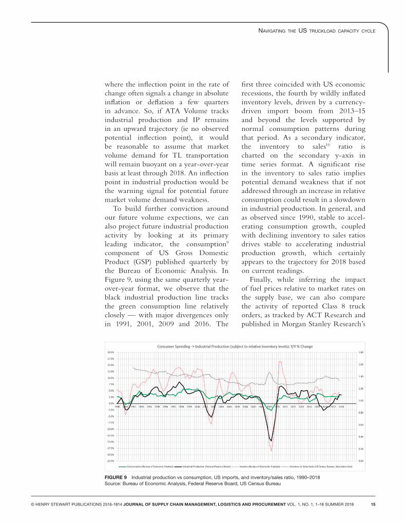
To build further conviction around our future volume expections, we can also project future industrial production activity by looking at its primary leading indicator, the consumption9 component of US Gross Domestic Product (GSP) published quarterly by the Bureau of Economic Analysis. In Figure 9, using the same quarterly year-over-year format, we observe that the black industrial production line tracks the green consumption line relatively closely — with major divergences only in 1991, 2001, 2009 and 2016. The

first three coincided with US economic recessions, the fourth by wildly inflated inventory levels, driven by a currency-driven import boom from 2013–15 and beyond the levels supported by normal consumption patterns during that period. As a secondary indicator, the inventory to sales10 ratio is charted on the secondary y-axis in time series format. A significant rise in the inventory to sales ratio implies potential demand weakness that if not addressed through an increase in relative consumption could result in a slowdown in industrial production. In general, and as observed since 1990, stable to accel-erating consumption growth, coupled with declining inventory to sales ratios drives stable to accelerating industrial production growth, which certainly appears to the trajectory for 2018 based on current readings.

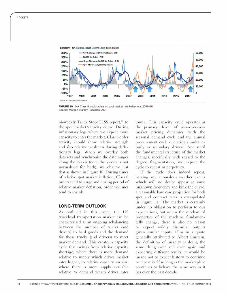
Finally, while inferring the impact of fuel prices relative to market rates on the supply base, we can also compare the activity of reported Class 8 truck orders, as tracked by ACT Research and published in Morgan Stanley Research’s

FIGURE 9 Industrial production vs consumption, US imports, and inventory/sales ratio, 1990–2018Source: Bureau of Economic Analysis, Federal Reserve Board, US Census Bureau

Pickett


bi-weekly Truck Stop/TLSS report,11 to the spot market/capacity curve. During inflationary legs where we expect more capacity to enter the market, Class 8 order activity should show relative strength and also relative weakness during defla-tionary legs. When we overlay both data sets and synchronise the date ranges along the x-axis (note the y-axis is not normalised for both), we observe just that as shown in Figure 10. During times of relative spot market inflation, Class 8 orders tend to surge and during period of relative market deflation, order volumes tend to shrink.

LONG-TERM OUTLOOKAs outlined in this paper, the US truckload transportation market can be characterised as an ongoing rebalancing between the number of trucks (and drivers) to haul goods and the demand for those trucks (and drivers) to meet market demand. This creates a capacity cycle that swings from relative capacity shortage, where there is more demand relative to supply which drives market rates higher, to relative capacity surplus, where there is more supply available relative to demand which drives rates

lower. This capacity cycle operates as the primary driver of year-over-year market pricing dynamics, with the seasonal demand cycle and the annual procurement cycle operating simultane-ously as secondary drivers. And until the fundamental structure of the market changes, specifically with regard to the degree fragmentation, we expect the cycle to repeat in perpetuity.

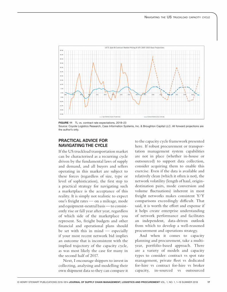
If the cycle does indeed repeat, barring any anomalous weather events which will no doubt appear at some unknown frequency and kink the curve, a reasonable base case projection for both spot and contract rates is extrapolated in Figure 11. The market is certainly under no obligation to perform to our expectations, but unless the mechanical properties of the machine fundamen-tally change, there is also no reason to expect wildly dissimilar outputs given similar inputs. If as in a quote generally attributed to Albert Einstein, the definition of insanity is doing the same thing over and over again and expecting different results, it would be insane not to expect history to continue to repeat itself so long as the marketplace continues to behave the same way as it has over the past decade.

FIGURE 10 NA Class 8 truck orders vs spot market rate behaviour, 2007–18Source: Morgan Stanley Research, ACT



PRACTICAL ADVICE FOR NAVIGATING THE CYCLEIf the US truckload transportation market can be characterised as a recurring cycle driven by the fundamental laws of supply and demand, and all buyers and sellers operating in this market are subject to these forces (regardless of size, type or level of sophistication), the first step to a practical strategy for navigating such a marketplace is the acceptance of this reality. It is simply not realistic to expect one’s freight rates — on a mileage, mode and equipment-neutral basis — to consist-ently rise or fall year after year, regardless of which side of the marketplace you represent. So, freight budgets and other financial and operational plans should be set with this in mind — especially if your most recent network bid implies an outcome that is inconsistent with the implied trajectory of the capacity cycle, as was most likely the case for many in the second half of 2017.

Next, I encourage shippers to invest in collecting, analysing and modelling their own shipment data so they can compare it

to the capacity cycle framework presented here. If robust procurement or transpor-tation management system capabilities are not in place (whether in-house or outsourced) to support data collection, consider acquiring them to enable this exercise. Even if the data is available and relatively clean (which it often is not), the network volatility (length of haul, origin-destination pairs, mode conversion and volume fluctuations) inherent in most freight networks makes consistent Y/Y comparisons exceedingly difficult. That said, it is worth the effort and expense if it helps create enterprise understanding of network performance and facilitates an independent, data-driven outlook from which to develop a well-reasoned procurement and operations strategy.

And when it comes to capacity planning and procurement, take a multi-year, portfolio-based approach. There are a variety of models and capacity types to consider: contract vs spot rate management, private fleet vs dedicated for-hire vs contract for-hire vs broker capacity, in-sourced vs outsourced

FIGURE 11 TL vs. contract rate expectations, 2018–23Source: Coyote Logistics Research, Cass Information Systems, Inc. & Broughton Capital LLC. All forward projections are the author’s only.

Pickett


procurement and execution, etc. All available alternatives should be considered during the planning process and leveraged to optimal advantage through the capacity cycle over the long term. The deflationary leg of the cycle creates unique opportunities and challenges relative to the inflationary leg, and vice versa. This dynamic should be considered when planning and executing any capacity strategy that is expected to perform over the long term.

Finally, one should always endeavor to be a shipper of choice — not only when inflationary market conditions dictate it. The best way to achieve relative consistency and stability through the capacity cycle is through consistent and stable long-term partnerships, based on mutual trust and a shared under-standing of risk. Decide who you want to do business with over the long term, and who want the same from you, and engage them accordingly. Create and sustain an operational environment that minimises idle time for drivers and other staff, maintains a safe and comfortable experience during pick-up and delivery, and allows for the network flexibility needed to absorb the frequent disrup-tions inherent to the real world.

REFERENCES(1) Armstrong & Associates, Inc. (October 2017),

‘Global and Regional Infrastructure, Logistics Costs, and Third-Party Logistics Market Trends and Analysis’, pp. 33, 44, available at http://www.3plogistics.com/product/global-regional-infrastructure-logistics-costs-third-party-logistics-market-trends-analysis/ (accessed 14th May, 2018).

(2) American Trucking Association, Reports, Trends, & Statistics, available at http://www.trucking.org/News_and_Information_Reports_Industry_Data.aspx (accessed 14th May, 2018).

(3) Based on 2017 Total Revenues relatives to estimated 2017 US trucking market size, ‘Transport Topics 2017 Top 100 For-Hire Rankings’, available at http://www.ttnews.com/top100/for-hire/2017 (accessed 14th May, 2018).

(4) Cass Linehaul Index, Cass Information Systems, Inc. & Broughton Capital LLC, available at https://www.cassinfo.com/transportation-expense-management/supply-chain-analysis/transportation-indexes/truckload-linehaul-index.aspx (accessed 14th May, 2018).

(5) American Trucking Association, Inc. (March 2018), ‘Trucking Activity Report using Total Truckload, Loads, Seasonally Adjusted’, available at http://www.foodshippersofamerica.org/files/2018%20Presentations/Session%204%20Annual%20Economic%20Update.pdf (accessed 14th May, 2018).

(6) U.S. Energy Information Administration, ‘US On-Highway Diesel Fuel Prices (dollars per gallon)’, US National Total, available at https://www.eia.gov/petroleum/gasdiesel/ (accessed 14th May, 2018).

(7) US Industrial Production (US Federal Reserve Board), available at https://www.federalreserve.gov/releases/g17/Current/default.htm (accessed 14th May, 2018).

(8) US Imports (US Bureau of Economic Analysis), available at https://www.bea.gov/iTable/iTable.cfm?reqid=19&step=2#reqid=19&step=2&isuri=1&1921=survey (accessed 14th May, 2018).

(9) US Consumption (US Bureau of Economic Analysis), available at https://www.bea.gov/iTable/iTable.cfm?reqid=19&step=2#reqid=19&step=2&isuri=1&1921=survey (accessed 14th May, 2018).

(10) Manufacturing & Trade Inventories & Sales (US Census Bureau), available at https://www.census.gov/mtis/index.html (accessed 14th May, 2018).

(11) Morgan Stanley Research (2018), ‘Truckload Freight Index Note May 2’, p. 5.

Documents

Navigating the US truckload capacity cycle: Where are ... · development and consulting roles at Adjoined Consulting (now Capgemini), Agile Software Corp. (now Oracle), Electron Economy