Embed Size (px)
Citation preview
AD-A260 379
NAVAL POSTGRADUATE SCHOOLMonterey, California
J".DTICGR E 2 2 19931
THESIS
MULTIPLE-VALUED PROGRAMMABLELOGIC ARRAY MINIMIZATION BY CONCURRENTMULTIPLE AND MIXED SIMULATED ANNEALING
by
Cem Yzldzrzm
December, 1992
Thesis Advisor: Jon T. ButlerSecond Reader : Chin-Hwa Lee
Approved for public release; distribution is unlimited.
93-03647 98 2 rz].
Kri ttKiTS Cl.%SSIF1('ATI0N OF FIllS PAGE
REPORT DOCUMENTATION PAGE 01P No 0-4-OISd
la RKPowr %Fi:I*RITX CL1ASSIFICATION lh. RE'srRIC 115 \I. ARKINGS1 nclassafl, d
2a. SECI RITN CLASSIFICATION At CIIORIl ' 3.DlISTRIBITI1ON 55 AK!.sItIIII s OF REPORTAppros ed for public rekeas; distribution is unilimited.
2h. IDECLIASSIFICATION.sDO\\NGRADING SCHEDULIE
4 PERFORMINC ORG~ANIZ.TION REPORT NUMIBER(S) 5. MON11 ORING ORGANIZATION REPORT NUM'\BER(S)
NAF OF PERFORAUNG ORGANiZATION 6b. OFFICE SYMBOL %. NAME OF MON'II ORIN(; OR(;.ANIZATlIONas L Psgraduate School o/appliable) Natal Postgraduate School
1 32
,,c .!)1)R FS (Cit%. State. and ZIP Code) -b. ADIRESS (('it%. StAte. and ZI' Co~de)\IontercN. CA 93943-5000( %lonterr%. C.A 93943-400lf,
Ra. N.VII or FUNDING SPONSORING fSb. OFFICE SYMBOL. 9. PROCU-RE\IENTI INSTRUMIENTnI)El~ 'FIC ATION NUM\BERORGANIZATION ttapplicable)
8c. A))SSCt.State, and ZIP Code) 10OSOURCE OF FUINDING NUMBERS
PROG RAM PROJECT TAKNOWORK UNIT
ELEMENT NO NO ACCESSION
i fi urF tinciude securizi (lassifit-ationiit.a ':k d Programmabl~he Logic Arra% Mlinimization It% Concurrent Multiple and Mixted Simulated. Ann ealing
*. ?i7US1 NAL AUTH-OR(S) Cern Yidtrini
13I a.'N illP OF REPORT 13b. TIME CONVERED 1 4. )ATEF Of R EPORT icYear. Month. DaY) j15. PAGE COUNTk \lastur' I hesis F-ROM ______TO ______1992 Diecenmber It) 60
The sies's expressed in thi, thesis are those of the author and do lnot reflect official poIie% or position or the Department ol IDefense or the U.S. Government
17. (OSATI CODES 18. SUB.JFCT TERMIS (Continue on reverse lf necvssaryi and identify kr blork number)
K IF IA) GROUP SUB-GROUP Multi-Valued Logic; Minimization Heuristics; PL.A Design; Simulated Annealing
19..SBSTR.ACT (Contmuit oi re'erse if necessary and identif) hi block number)
The prrocess of finding a guaranteed minimal solution for a multiple-s alued programmable logic expression requires an exhaustive search. Exhausti,.est-rc is not %cry realistic because of enornious computation time required to reach a solution. One of the heuristics to reduce this conmputation time and
1prin idu a near-minimal solution is simulated annealing.'I his thvsis analvzes the use of loose] % -cou pled. course-2rained parallel systenms for simulated annealing. This approach insolses the use ofmnultiple pro-
cvss..rs 1%shtre interproress conununication occurs einl% at the beginning and end If the process. In this studN, the relationship betwAeen the qualit- of solu-l'ion. mrivsured bi the number of products and computation time, and simulated annealing paranmeters art, inestigated. A sinmulated annealing experiment-salso ill, estigatedn~he-re tiso types of moses are mixed. These approaches prosidt, impros ement in both the number (Ifproduct terms and computation:ime-.
1211, I)IS-1IM-BTIONIAVAILABILITY OF ABSTRLACT 21. ABST ARCT SE('IRITI (1ASSIFICATIONI tNCLASSIFIEDMtNLIMITED F1 SANIE AS REPORT DTIC USERS Unclassified
'2a. NAME 0OF RESPONSI BILE IN"DIVIDU AL 22b. TELEPHONE (int-lude. Irea Code) 22c. OFFICE S1 NBOL
SEFCURITIYCL .tSSIFIC'(ATION OFTIls pAc;FE. ra -(3II 86Previous e'ditions art, obsolete t nclassifled
%/N tII02.1,Ft)14-411AI3
Approved for public release: distribution is unlimited.
Multiple-Valued Programmable Logic Array MinimizationBy Concurrent Multiple and Mixed Simulated Annealing
by
Cem YildirimLieutenant Junior Grade, Turkish Navy
B.S., Turkish Naval Academy, 1985
Submitted in partial fulfillmentof the requirements for the degree of
MASTER OF SCIENCE IN ELECTRICAL ENGINEERING
from the
NAVAL POSTGRADUATE SCHOOLDecember 1992
Author: __
Cern Yildirim
Approved by: -FJnT. Butler, Thesis Advisor
--inwa e, Second Reader
Michael A. Morgan, Chai hanDepartment of Electrical and Computer Engineering
ABSTRACT
The process of finding a guaranteed minimal solution for a multiple-valued
programmable logic expression requires an exhaustive search. Exhaustive search is
not very realistic because of enormous computation time required to reach a
solution. One of the heuristics to reduce this computation time and provide a near-
minimal solution is simulated annealing.
This thesis analyzes the use of loosely-coupled, course-grained parallel systems
for simulated annealing. This approach involves the use of multiple processors where
interprocess communication occurs only at the beginning and end of the process. In
this study, the relationship between the quality of solution, measured by the number
of products and computation time, and simulated annealing parameters are
investigated. A simulated annealing experiment is also investigated where two types
of moves are mixed. These approaches provide improvement in both the number of
product terms and computation time.
DTIC QUALmTy rNSPFCTED
Aoessi.Io r --mw
i NTIS GRA&I .DTIC TAB 0Unannounoed 0
ZB-.---_
Availabillity Codeg
Dist Special
TABLE OF CONTENTS
I. INTRODUCTION ........................................... 1
A. MOTIVATION .. ..................................... 1
B. BACKGROUND . .................................... 4
II. NEW APPROACHES FOR SIMULATED ANNEALING ............ 7
A. DIFFERENT PATHS .................................. 7
B. ANNEALING WITH MIXED MOVES ................... 10
C. CONCURRENCY IN SIMULATED ANNEALING WITH
MULTIPLE AND MIXED MOVES ...................... 12
III. OPTIMUM PARAMETERS FOR CONCURRENT AND MIXED
SIMULATED ANNEALING ............................... 16
IV. EXPERIMENTAL RESULTS ................................ 19
V. CONCLUSIONS .......................................... 25
VI. APPENDIX A: FLOW DIAGRAM OF THE ALGORITHM ....... 27
iv

V. APPENDIX B: C CODE UTILIZED .......................... 29
LIST OF REFERENCES ....................................... 50
INITIAL DISTRIBUTION LIST .................................. 52
V
ACKNOWLEDGEMENT
I would like to express my sincere appreciation to the Turkish Navy and
United States Navy for providing this exceptional educational opportunity. In
appreciation for their time and effort, many thanks go to the staff and faculty of the
Electrical and Computer Engineering Department, NPS. A special note of thanks
goes to Dr. Yang for his support and guidance. I would like to offer special thanks
to my advisor Dr. Butler for his guidance and encouragement.
vi
1. INTRODUCTION
A. MOTIVATION
In the last ten years. significant progress has been made in realizing large logic
circuits in silicon using very-large-scale-integration (VLSI) technology. With this
progress there have been two major problems, interconnection and pin limitation.
Indeed, they have become bottlenecks to further integration. Multiple-Valued-Logic
(MVL) offers a solution. In MVL, there are more than two levels of logic. MVL has
found application in programmable logic arrays (PLA) implemented in
charge-coupled devices (CCD) [Ref. 1,2,3,4] and current mode CMOS [Ref. 16,17].
Several heuristic algorithms have been developed related to computer-aided
design and logic synthesis tools for multiple-valued PLA's [Ref. 5.6,7,8,9,14,15,16,17].
None of these heuristic algorithms is consistently better than the others [Ref. 9],
each having an advantage in specific examples [Ref. 5,6,7,8,9]. Heuristic algorithms
are important because algorithms that guarantee a minimal solution require
exhaustive search. Exhaustive search is not very realistic due to the immense amount
of computation time required to reach a solution.
A new heuristic, simulated annealing, offers a solution for obtaining near-
minimal solutions to combinatorial optimization problems with reasonable
computation times. Advantages of this technique include its potential to find true
minimal solutions, general applicability, and ease of implementation [Ref. 12].
1I
- -
Because of the similarity to the statistical mechanical model of annealing in solids
this technique is called "simulated" annealing. That is, the slow cooling of certain
solids results in a state of low energy. a crystalline state, rather than an amorphous
state that results from fast cooling.
Simulated annealing is a search of the solution space in a combinatorial
optimization problem. Its goal is to find a solution of minimum cost with the
repeated application of the following three steps [Ref. 12].
1) Create a new solution from the current solution: In this step, the algorithm
chooses a pair of product terms, and tries to make a move to reach to a new
solution. If the two product terms can be combined into one, they are combined.
This is called a cost decreasing move. If they can not be combined, the two are
replaced by two or more equivalent product terms. If indeed, there are two new
product terms a zero-cost move is proposed. If there are three or more product
terms, a cost increasing move is proposed.
2) Calculate the cost of the new solution: This step calculates the cost of the
move by comparing the number of product terms before and after the move.
3) If the increase in cost of the new solution is below some specified threshold,
it becomes the current solution: The algorithm decides if the move is accepted or
rejected, depending on the threshold which is a function of the cost and the current
temperature.
Unlike other minimization techniques (which are classified as direct-cover
methods), simulated annealing manipulates product terms directly, breaking them
2
up and joining them in different ways to reduce the total number of product terms.
Manipulation of product terms is done nondeterministically. That is. randomly
chosen product terms are randomly combined (cost decreasing move), reshaped or
divided (cost increasing moves). As with the mechanical applications of annealing,
the solution set is heated first and than allowed to cool slowly in order to reach a
crystalline state or optimum solution. Given an expression in the form of a set of
product terms, the algorithm [Ref. 11] divides and recombines the product terms,
gradually progressing toward a solution with fewer product terms. Although cost
increasing moves represent movement away from the optimal solution, they allow
escape from local minima. The repeated application of the three steps above usually
requires a large number of moves before a minimal or near-minimal solution is
achieved. Therefore, a bias is applied which determines the probability of acceptance
of cost increasing moves. Initially, the probability of accepting such a cost increasing
move is high, between 0.5 and 1.0. However, as the cooling starts, this probability
decreases. As a result, at the beginning, wide excursions are made in the solution
space, while near the end, only global or local minima explored. When the
probability of accepting a cost increasing move is very low, simulated annealing is
usually in a global or local minima, which indicates that the probability of escape is
also low. Thus, if the probability is decreased quickly (a process called quenching),
simulated annealing converges on a local minima with little chance of escape. A
preferred approach is to decrease the probability of accepting cost increasing moves
3
slowly, which means a slow cooling. This allows transitions among more states and
improves the chance of finding a global minimum.
A brief review of the minimization problem of an MVL PLA is given below.
Then, a new implementation of simulated annealing is presented.
B. BACKGROUND
A product term is expressed as
x aX1b X 2 .... a (1.1)
where c e{1,2, ...,r-1}, is a nonzero constant, where the literal function is given as
,Xb, { r-1 a, g x, ! bo (1.2)
and where concatenation is the min function; i.e. xi=min(x.y). Since the literal
function takes on only values 0 or r-1, the product of literals is either 0 or r-1, while
the complete term takes on values 0 or c. An r-valued function f(x1,x- ...,xn) takes on
values from {1,2,..,r-1} for each assignment of values to the variables, which are also
r-valued; i.e. xi E {0,1,2,...,r-1}. A function can be represented by sum of these
products as follows
ftX1,X2,_..,x.) = C1 a,,, 1 bu al.2bi.2 a1 ~x bi.X
+c2 x1 x2 ... xn (1.3)
4

where + is truncated sum. i.e. a+b = max{a+b . r-l}, where the right sum is
ordinary addition with a and b viewed as integers.
A minimum sum-of-products expression for f(x,.x,._x,,) is the one with the
fewest product terms. Finding such a solution is based on that shown in Dueck et
al [Ref. 11]. Given a set of product terms that sum to a given function, the
algorithm derives another set by making a move. Similarly, a move is made from the
next set, etc. until finally a minimal or near-minimal set is formed. As in [Ref. 11],
this thesis investigates two kinds of moves.
1) Cut-or-Combine: The two randomly chosen product terms are combined
into one, if possible. If not, one is chosen randomly, with probability 0.5. If the
chosen product term is a I minterm (i.e. a product term of the form
lalbi, a•xx 2 .... a x, where a,=hi for all i). the current move is abandoned and
another pair of product terms is chosen. Otherwise, the chosen product term is
divided into two. The process of division occurs either along the logic values or
geometrically. If the division is along the logic value, the resulting product terms are
the same except for their constant c values which sum to the logic value of product
term. If the division is done geometrically, the two product terms have the same
constant c value and are adjacent, covering all minterms covered by the original
product term.
2) Reshape: This movt, like Cut-or-Combine, operates on two product terms,
and combines the pair if a combine is possible. If not, a consensus term is formed.
5
If the two product terms overlap, the consensus is the intersection of the two terms
with a coefficient that is the truncated sum of the two coefficients. If the two
product terms are disjoint (but adjacent), then the consensus is a term taking on two
parts of two product terms, with a coefficient that is the minimum of the two
product terms. The remaining product terms are chosen so that the fewest number
cover all minterms covered by the original product term.
In this thesis, instead of committing to either Cut-or-Combine or Reshape, a
mixture of both with different paths is used, and this is performed concurrently in
a distributed system. The results of the following three different approaches are
investigated:
1) Different paths in the solution space.
2) Mixing types of moves.
3) Concurrency.
These methods are explained in Chapter II. Experimental results of concurrent
multiple and mixed simulated annealing are summarized in Chapter III. Concluding
remarks are given in Chapter IV.
6
I1. NEW APPROACHES FOR SIMULATED ANNEALING
In the early stages of this thesis, two techniques for the parallelization of
simulated annealing for MVL PLA minimization were considered:
1) Speculative simulated annealing proposed by Witte el al [Ref. 10] : This
technique provides speedup only when the cost evaluation time is large compared
to the move generation time. This is not the case of our problem, and this approach
was abandoned.
2) The division algorithm : This algorithm which is an approach to fine-grained
parallelism was also abandoned because the original algorithm was efficiently
written, and fine-grained parallelism provided only marginal improvement.
As a result of this experience, we concentrated on course-grained parallelism,
in which there is minimal communication among processes.
A. DIFFERENT PATHS
During the simulated annealing process, the algorithm randomly walks through
the solution space. A random walk through solution space will eventually result in
a minimal solution, if there is a nonzero probability of reaching the minimal solution
from any other solution. This is one way to achieve a minimal solution with
probability approaching 1.0 as time increases. But it is impractical, because of
excessive computation time. Simulated annealing uses a different technique for
7

random walk in which the probability of transition to a higher cost solutions
continually decreases toward 0. In this technique, like a random walk, the transition
from one solution to another occurs randomly. But unlike random walk, the
transition probability is not uniformly distributed among all possible next solutions.
It is biased toward lower cost solutions, with the bias increasing as time passes. Fig.
2.1 shows this. All squares in a column represents solutions with the same number
of product terms. Columns on the right represent solutions with large
<= COST DECREASING MOVES COST INCREASING MOVES
RESULT 2 *m ~~E *
S m.mmm STARTING
TWO POSSIBLE if0 GLOBAL a U 0 0 0 m
MINIMA
wu THREE POSSIBLE - * i mN LOCAL MINIMA - "" -.
U -- -
L U
RESULT 1
Figure 2.1: Examples of simulated annealing using different paths.
number of product terms. Squares on the extreme left represent local minima. The
algorithm can make three types of moves, cost decreasing, cost increasing and zero-
8
cost moves, represented by right going. left going and vertical arrows, respectively.
As the time passes, with the decreasing probability of cost increasing moves, it
becomes less likely that a move is made away from the optimal solution. The two
paths in Fig. 2.1 shows two examples of simulated annealing experiment. One results
in a nonoptimal solution, while the other results in an optimal solution.
Fig. 2.1 also illustrates one approach we considered, different paths. This
approach was tested using the Reshape algorithm on ten different functions
(C1,C2,..,C10) which were used in Dueck et al [Ref. 11]. Each function has 200
minterms. For every function, eight different paths were chosen. Table 2.1 shows the
results. The column "FUNCT' shows the different test functions. The columns under
the terms "PATH" show the results of the different paths. Each entry shows two
results, the number of product terms achieved and the computation time (in
parentheses) in seconds. The computation time is CPU seconds on Sun Workstation
running the SunOS Release 4.1.1-GFX-Rev2 operating system. The column "OUT'
shows the lowest number of product terms. This is considered to be the output of
the algorithm. In this column, parentheses enclose the total computation time over
the eight paths. Since this was performed on one processor, this total is the
computation time for this (sequential) version of the algorithm. The average values
of product terms and computation times for each path are given in the second to the
last row. As we see from Table 2.1, there is a clear dependence on the path. For
example, the eight paths on function C4 yield five different values for a near-
minimal solution, 80, 81, 82, 83 and 86 product terms.
9
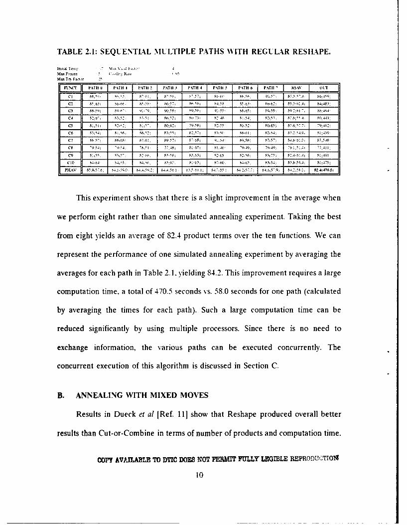
TABLE 2.1: SEQUENTIAL MULTIPLE PATHS WITH REGULAR RESHAPE.
lnifiaý Tetmp ,." Max \'n alo4
MaxuFrzn 5 (,,,.ln. R,,;e 5 '3Max Ti% Facior 25
n-% I PATH 0 J PAT11 I[ PATH 2 PATHS 3 PATH 4 J PATHS I PATH 6 J PATHS RSAV I 1M
C 1 88$ ý s'I 3'I "I" (7 1 r',56, ý- 65 , f6.6 $6 s 56; 90, 5-, 67.3i5- 86'545'I
C:2 85t635 S6.66. s'5,56, 86,57, S6 56; 64.5$5, 95 (63) 866261 85.3,6 O.4j 84(483)
C3 S: 591 RQr67, 91,-9, 90,5s; 9.56; 4.55 S8 b65 84 ;(55 5 9.2K61- , 8, 494,
C4 352, 3:51 86,52 Sri: 731 N: 48F 81,54) 25,53 82.S55 4, 80.443,
C5 8 511 152,': 1•,5, 8 1 6 79,58; 8F.55; S052, 90(65) 8,.6.57.7 79t46:)
C6 S3,54-:' ; •156, 96,52 , 83.55 St57; 6) "5;5, S6,61 82i54; 8.2,54.9, S1)459ý
C7 9$ 57, 88,,,g $7.61, 89,57, 87,681 ?I.5, 9,58 r 87,57) S.4.861.V.0; 87,548,
C8 '954- 95-, 78.51 , 77,45, 81.60 -146) '9,39) 79t49) 79.1,51.4- 70411
C'9 8155 S3,5 ', 2'66, 83,56; 88-6'; $263 S2;56) 8373I 82.4,61.11 $11491
C S4,6. 54,55 84,5)., S3(6$; , $1.63; I 6. 6 5'-;, 4 , F85.5 8., 59.4. SI1475)
P'AV .9,57.6) 64.1 59.0, S•-4 59.-• k4.4'56': , ;. 5 61.1 $14.7, 55.1 84 2,57.7) S4.1 (5- 7 4. 58. 82.4450.ý51
This experiment shows that there is a slight improvement in the average when
we perform eight rather than one simulated annealing experiment. Taking the best
from eight yields an average of 82.4 product terms over the ten functions. We can
represent the performance of one simulated annealing experiment by averaging the
averages for each path in Table 2.1. yielding 84.2. This improvement requires a large
computation time, a total of 470.5 seconds vs. 58.0 seconds for one path (calculated
by averaging the times for each path). Such a large computation time can be
reduced significantly by using multiple processors. Since there is no need to
exchange information, the various paths can be executed concurrently. The
concurrent execution of this algorithm is discussed in Section C.
B. ANNEALING WITH MIXED MOVES
Results in Dueck et al [Ref. 11] show that Reshape produced overall better
results than Cut-or-Combine in terms of number of products and computation time.
Copy AVjLAWLE TO DTIC DOES NOT PEPRMIT FULLY LEGIBLE REPRODUCTTON
10
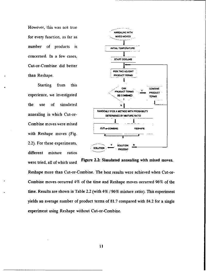
However, this was not trueANNEALING WITH
for every function, as far as MIXED MOVES
number of products is INITIAL:NTALTEMPERATURE
concerned. In a few cases,START COOLING
Cut-or-Combine did betterPICK TWO ADJOINT
than Reshape. PROoDUCT TERMS
Starting from this COMBINE
PRODUCT TERMS Y PRODCTexperience, we investigated -BE COMBINED TERMS
the use of simulated N
RANDOMLY PICK A METHOD WITH PROBABILITY
annealing in which Cut-or- DETERMINED BY MIXTURE RATIO
Combine moves were mixed ISACUT-or.COMBINE RESHAPE
with Reshape moves (Fig. _-.
2.2). For these experiments, • Y souToN NSOUTION -'FROZEN?
different mixture ratios
were tried, all of which used Figure 2.2: Simulated annealing with mixed moves.
Reshape more than Cut-or-Combine. The best results were achieved when Cut-or-
Combine moves occurred 4% of the time and Reshape moves occurred 96% of the
time. Results are shown in Table 2.2 (with 4% / 96% mixture ratio). This experiment
yields an average number of product terms of 81.7 compared with 84.2 for a single
experiment using Reshape without Cut-or-Combine.
11

TABLE 2.2: SEQUENTLAL MULTIPLE PATHS WITH MIXED ANNEALING.
Initial Temp M&% \ ,UI': I
Max Frozen 5 ()olinc R.,:,
MuTry Fator 5 ('-,r-(.'::u,: R-,.a:',• R",iU 4") qt,
F RAVG PATH 0 PATH I PATH 2J PATH J1 [PATH 4 PATH 5 PATH 6 PATH 7 __'_
C1 87.3(57.4t 8M(5?7 ! 7.7, S4,$91 S6, & r t 'F-) 87)63) 89f93) W,.66) F4(562)
C2 85.3(60.4p 8 3
(6 6
k s5' ss 3! , .91, &84,78) 86-73) 85(96, 85 t 76) 8. 51)
C3 89.2(61.7i 88))97 89ý90, $9 9.; F9,--, 89(6b' 87(79) 89179) 89(83) 87K672)
C4 82.8(55.4i 82163) 82:, L 1!491 7$ 53, 83(53) 80(58) 85(62) 81(61) 786491)
CS 80.6(57.7) 80(91 F9-; $277, K",7I 82!77) 82(92) 82(73) 80t61 79(577)
C6 83.2)54.91 83(70, 8263, $361 8296, 86j67 84(58) 83(61) j 4(59) 8K,562)
C7 &4.8(60.0) 87t6), 8b,• $7,671 8899 86(671 91A80) 88(891 8W,108) 86,671 i
C8 79.1(51.4 7867 .7(, 79;(84, 7891. 78,55, 77)69) 76.6fl 79(70, 76802)
C9 82.461 K. F7 S-•SS S5 91, 8( 63
1 84(67) 83(6) 83 i87 8,!06017 )
CIO 83.8(59.4, 82: -, F S5: ', 84C 5. 83(63, 85(71) 8'3 84b 864 8 96)
AVRG 8"4.2)580 83434 ., 6.8 .- ) 53..2 6) 83.9(66.8, 4N3(71.0) 84.3(75.2) 84.3(18, 81.798.1
C. CONCURRENCY IN SIMULATED ANNEALING WITH MULTIPLE AND
MIXED MOVES
It has been shown that the use of more than one path with and without mixed
moves provides a reduction in the number of product terms over the use of one
path. However, substantial computation time is required when one processor is used.
But using more than one processor in a distributed system, we can achieve a
speedup. To investigate this, eight Sun Workstations were used. Fig. 2.3 shows the
program for this distributed system. In the beginning, the host sends the name of the
file (in which input function is placed) to the other processors and later assigns itself
as processor 0. Since multiple path and mixed simulated annealing is suitable for
execution on asynchronous multiple instruction multiple data (MIMD) machines,
each workstation can proceed independently of the others. In this algorithm, each
processor chooses the paths randomly. Assigning different seeds for the random
M &VMILABLE TO DTIC DOES N0T PERMIT FULLT LEoIBLE MPRODUCTMON
12

.. CONCURRENTMULTIPLE & MIXED
\ SIMULATED
SANNEAUNG
ASSIGN FUNCTION
AND STARTING POINTS ,___1 1 111 1I
PROCEMSORO PROCESSOR I PROCFSSORT7"
MIXED SIMULATED MIXED SIMULATED ----. MIXED SIMULATED
ANNEAUNG ANNEALING ANNEALINGI 1-----1 1 1 1
COLLECT SOLUTIONSFROM PROCESSORS
PICK THE BEST OUTPUT
SOLUTION
Figure 2.3: Concurrent implementation of multiple path with mixedmoves.
number generators of the processors reduces the probability of two processors
picking identical next solution states. The probability that two or more processors
choose the same pair of product terms can be calculated as
1- ! , (2.1)
(M-N)! MW
where
M=(P) ,(2.2)
N is the number of processors used, and P is the number of product terms in the
function to be minimized. For instance, with 8 processors and a function with 200
product terms, this probability is 0.0014 . The probability of two processors going to
the same next state is even less, since even if they choose the same pair of product
13
terms, there is a choice of how to divide one of the two. Because of such a small
probability, the program does not check if two processors have started with the same
next solution state nor if at any point in the computation of the solution is the same.
This approach requires the communication only at the beginning and at the end of
the process. As soon as the host (processor 0) completes its own assignment, it starts
to receive the other processors's results when they are read), to be sent. As the final
result of the algorithm, the best output among all processes is chosen.
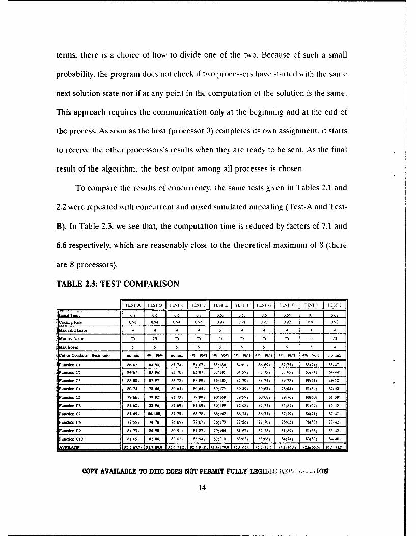
To compare the results of concurrency. the same tests given in Tables 2.1 and
2.2 were repeated with concurrent and mixed simulated annealing (Test-A and Test-
B). In Table 2.3, we see that, the computation time is reduced by factors of 7.1 and
6.6 respectively, which are reasonably close to the theoretical maximum of 8 (there
are 8 processors).
TABLE 2.3: TEST COMPARISON
rTEST A TEST B JTEST C TUST D fTEST-1E TEST F JTESI G TESI H TEST) I ET
Initial Temp 07 0.6 0.6 0.7 0.65 0.62 0.6 0.65 0.7 0.62
Cooling Rate 0.98 0.94 0.94 0.98 0.97 0.91 0.9. 0.92 0.91 0.92
Max valid factor 4 4 4 4 5 4 4 4 4
Max tir fctor 25 25 25 25 25 :5 25 25 20
Max frozen 5 5 5 5 5 5 5 5 4
Cin-or-Combine Resh ratio no tnix .1' no mix 4, 96% 4% 96, 4'¢ 96% 4% 96- 4% 96% 4% 96% no mix
Function CI 86(62) 94(9.) 85(74) 84(87) 851186) 84(61) 86)69) 87)75) 85171) 85(47)
Function C2 84(67) 83(96) 83)70) 83(87) 82(181) 84&59) 83(75) 85(85) 83)74) 84(44)
Function C3 88(80) 87197) 88(75) 88(89) 86(185) 87)70) 88(74) 89(78) 88(71) 89(52)
"unction C4 80(74) 78(65) 80(64) 80(64) 80(175) 80(59) 80)61) 78(65,) 81)54) 82(40)
Fumction C5 79(66) 79(92) 81(71) 79(88) 80(168) 79(59) 80(68) 79(76) 80(60) 81(39)
Function C6 81(62) 82(96) 82)69) 83(69) 80(189) 82f68) 8274) 83(81) 81)62) 83(431
Function C7 87169) 86(108) 87(75) 68078) 86(162) 86)74) 86(75) 87)79) 86(71) 87)42)
Function CS 77(55) 76(76) 78)69) 77(67) 76(179) 77(58) 77(70) 78(63) 78)53) 77(42)
Function C9 81(75) 90(9) 80191) 81)87) 79(164) 81(67) 8208) 81(89) 81)68) 83(41)
unction CIO 81(65) V.(86) 82(82) 83(941 82(210) 836.) 83(68) 84(74) 83(82) 8,448)
AV E2467. !..L 2 . 8. .L2, . 829'I64.0, 8'.7L71. 83.1176i 8.666 83.44.0
COPY AVAILABLE TO DTIC DOES NOT PERMIT FULLY LEGILLE MEPrN .... IOl
14
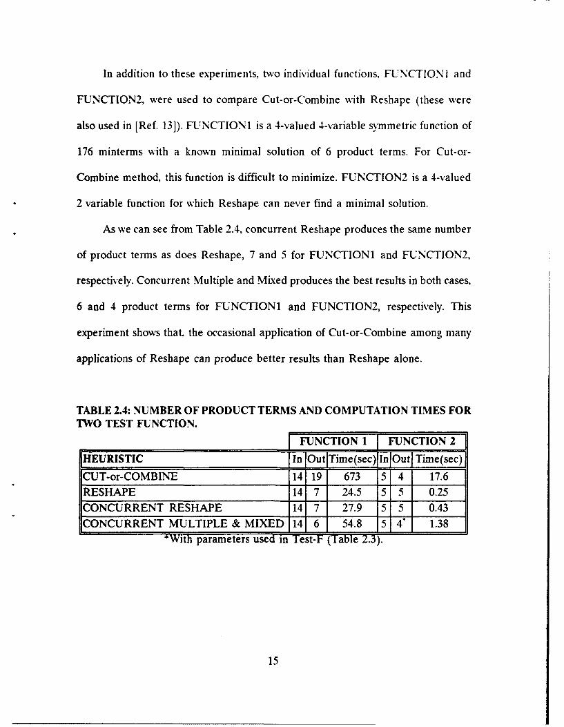
In addition to these experiments, two individual functions. FUNCTION I and
FUNCTION2, were used to compare Cut-or-Combine with Reshape (these were
also used in [Ref. 13]). FUNCTION1 is a 4-valued 4-variable symmetric function of
176 minterms with a known minimal solution of 6 product terms. For Cut-or-
Combine method, this function is difficult to minimize. FUNCTION2 is a 4-valued
2 variable function for which Reshape can never find a minimal solution.
As we can see from Table 2.4, concurrent Reshape produces the same number
of product terms as does Reshape, 7 and 5 for FUNCTION1 and FUNCTION2,
respectively. Concurrent Multiple and Mixed produces the best results in both cases,
6 and 4 product terms for FUNCTION1 and FUNCTION2, respectively. This
experiment shows that, the occasional application of Cut-or-Combine among many
applications of Reshape can produce better results than Reshape alone.
TABLE 2.4: NUMBER OF PRODUCT TERMS AND COMPUTATION TIMES FORTWO TEST FUNCTION.
FUNCTION 1 FUNCTION 2HEURISTIC [in [O-utFTime( sec )jIn I Out I Time( se~c)
CUT-or-COMBINE 14 19 673 5 4 17.6
RESHAPE 14 7 24.5 5 5 0.25
CONCURRENT RESHAPE 14 7 27.9 5 5 0.43
CONCURRENT MULTIPLE & MIXED 14 6 54.8 5 4" 1.38*With parameters used in Test-F (Table 2.3).
15
III. OPTIMUM PARAMETERS FOR CONCURRENT AND MIXEDSIMULATED ANNEALING
It is important to consider the effects of various parameters on the
performance of the methods discussed above. There are six important parameters
in the Concurrent Multiple and Mixed Simulated Annealing algorithm: Mixture rate.
cooling rate, initial temperature, maximum valid factor, maximum try factor and
maximum frozen factor.
Mixture rate determines the rate how two types of moves, Reshape and Cut-
or-Combine are mixed.
Cooling rate controls the number of temperatures that the process sequences
through during the transition from the melted to the frozen state.
Initial temperature controls the extent of melting. Since the temperature
directly controls the probability of accepting cost increasing moves, a higher initial
temperature means a more melted solution.
Maximum valid factor determines the number of moves occurring at each
temperature.
Maximum try factor regulates how long the program examines moves prior to
continuing on the next temperature. The number of attempted moves for each
temperature is calculated by multiplying the maximum try factor by the number of
moves.
16
Maximum frozen factor is used to determine if the process is really in frozen
state. This indicates that no more effort should be expended on the expression.
These parameters are tested with the following values.
a. Maximum frozen factor (3 : 4 . 5)
b. Maximum try factor (20 : 25 : 29 )
c. Maximum valid factor (3 : 4 ; 5)
d. Initial Temperature (0.50 : 0.55 : 0.60 ; 0.62 : 0.65 : 0.70 ; 0.75)
e. Cooling Rate (0.90 ; 0.91 " 0.92 ; 0.93 : 0.94 : 0.95 ; 0.97 ; 0.98)
f. Mixture Rate (Cut-or-Combine/Reshape) (109c/90% ; 5%4/95% ;4%/96%
3%/97% ; 2%/989c)
The effects of temperature dependent mixture rates are also investigated.
Using the current temperature, the mixture rate is changed as the time changes. This
approach did not give better results than the constant mixture rates.
There are almost 8,000 combinations of these parameters. However, this is too
many to evaluate experimentally. So, the following process is used to find a near-
optimum combination. At the beginning of the search, all values of "maximum
frozen factor" (3; 4; 5) are tested. During these tests, the remaining parameters (b,
c, d, e, f) are chosen to be the same as with Reshape in Table 2.1 (0.7; 4; 5; 0.93;
25), except that a mixture rate of 5%/95% is used. From these tests, the best value
(5) is chosen. Keeping this value, the second parameter (maximum try factor) is
searched and the best result (25) chosen. The rest of the search is done this way in
the order of given above for the parameters. After the first pass down to the last
17
parameter, another value is chosen for the third parameter and the search proceeds
as before. In this way, 70 passes were performed for each function across six
parameters.
Some of the results of these tests are given in Table 2.3. These are discussed
in Chapter IV.
18
IV. EXPERIMENTAL RESULTS
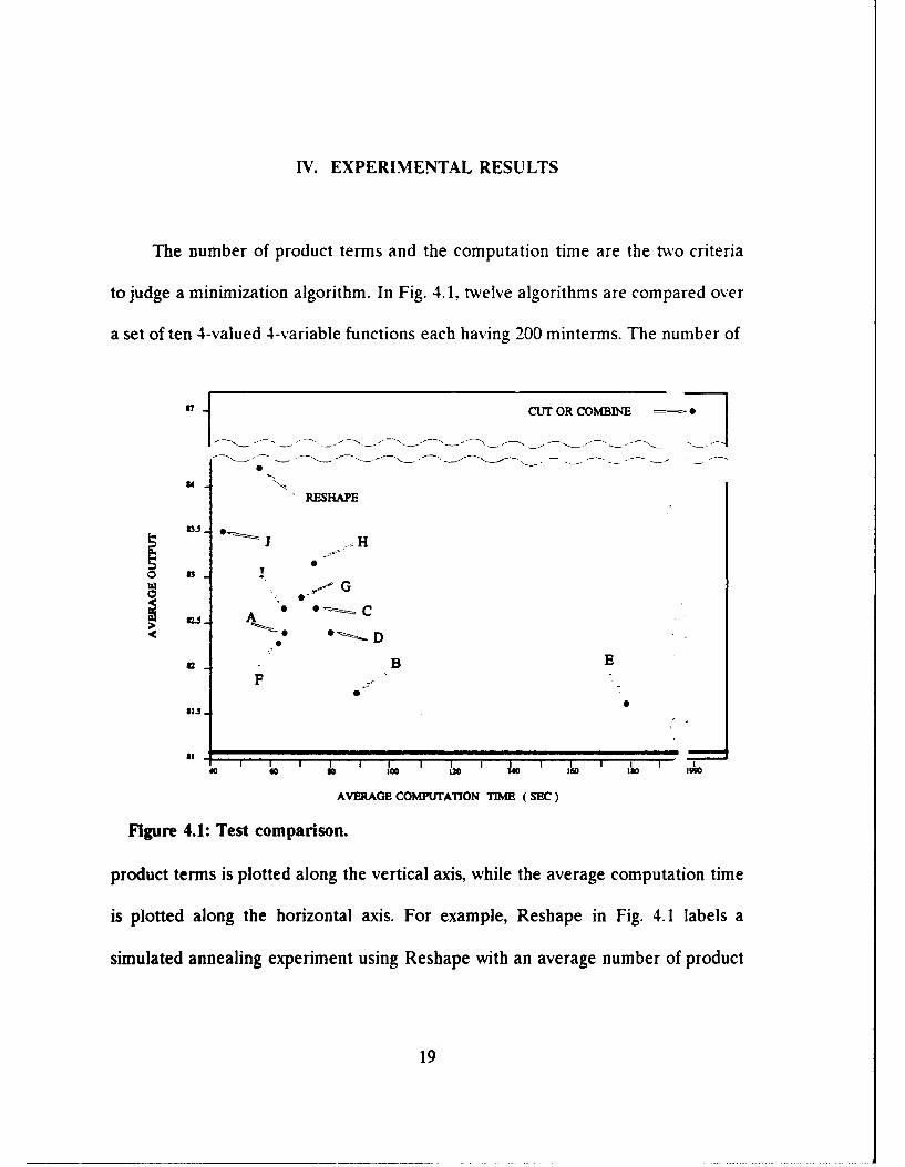
The number of product terms and the computation time are the two criteria
to judge a minimization algorithm. In Fig. 4.1, twelve algorithms are compared over
a set of ten 4-valued 4-variable functions each having 200 minterms. The number of
W7j CUT OR COMBINE
"RESHAPE33. "J H
0 !
S,..• G
B EF
S1S
I I I I I I I I 1 1I I I I l i f4o0 60 160 30 204 150 1i0 190
AVERAGE COMPUTATION TIM[E (SEC)
Figure 4.1: Test comparison.
product terms is plotted along the vertical axis, while the average computation time
is plotted along the horizontal axis. For example, Reshape in Fig. 4.1 labels a
simulated annealing experiment using Reshape with an average number of product
19

terms of 84.2 and an average computation of 58.0 seconds (the column RSAV in
Table 2.1). When Reshape is replaced by the Cut-or-Combine method in a single
simulated annealing experiment, we see that the result is a large number of product
terms (87.0) with a much longer computation time (1990.6 sec.). This point labelled
as Cut-or-Combine in Fi2. 4.1. It is far away from all other algorithms.
The point labeled A in Fig. 4.1 represents the experiment discussed in Section
II.C that uses the same parameters used in regular Reshape except that the
"concurrent multiple path" method is implemented. The result is an average of 82.4
product terms with a computation time of 67.5 seconds.
The point labeled D is an experiment (Table 2.3) that has the same parameters
as A. But in this experiment Cut-or-Combine and Reshape moves are mixed in the
ratio 4%/967'A. The result shows the same average number of product terms (82.4)
as in A, but the computation time (81.0 seconds) is worse. This shows that different
parameters may improve the result. This is tested as follows.
In the experiment labeled F (Table 2.3), the same mixture rate was used as in
D, with new parameters (0.62 initial temperature; 0.91 cooling rate). We see that
both the number of product terms and computation time are better than D. This
suggests that implementation of mixed annealing requires different parameters than
regular Reshape.
In the experiment labeled B (which has the concurrent and mixed method)
(Table 2.3), we obtained the best results in terms of product terms with reasonable
computation time. This shows that the parameters chosen for experiment labeled B
20

are close to optimum for concurrent and mixed annealing algorithm. The result is
an average of 81.7 product terms with a computation time of 89.9 seconds.
After the good results obtained from experiment labeled B, these same
parameters are tested in other cases. At first, these parameters are applied to
regular Reshape. In C, which is a regular Reshape with multiple paths (Table 2.3),
these same parameters produced worse results than A. This shows that the good
results produced by concurrent and mixed annealing are not just due to the choice
of parameters.
I is the same as F except that the initial temperature was chosen as 0.7 (as in
regular Reshape). The computation time is nearly the same, but average number of
product terms is worse.
Applying G and H (Table 2.3) also show how incorrect parameter selection can
affect the algorithms performance. In these cases, G is the same as B except that the
cooling rate is 0.92 instead of 0.94 and H is the same as G except that the initial
temperature is 0.65 instead of 0.60. This suggests that parameter selection is
important as a whole.
In applying J (Table 2.3), we intended to get a better average output than
regular Reshape, but with a faster computation time. In this test new parameters are
used (0.62 initial temperature; 0.92 cooling rate; 20 maximum try factor). Indeed this
test gave better results with fewer number of product terms and a shorter
computation time. Fig. 4.1 shows that J fell in the left lower side of the Reshape.
As expected, the number of product terms (83.5) was not better than 81.7 for B. But
21
there was a large improvement in computation time to 44.0 seconds compared to
89.9 seconds for B.
Fig. 4.1 also shows that there is a tradeoff between number of product terms
and computation time. The experiment labeled B seems the best in terms of average
computation time and output. That is why we picked it for "Concurrent Multiple and
Mixed Annealing" and used for the comparisons below. The solid line at 81.1
represents the best average output found, from all the tests done (approximately
700) with different parameters. This shows that there is opportunity in parameter
and mixture rate selection.
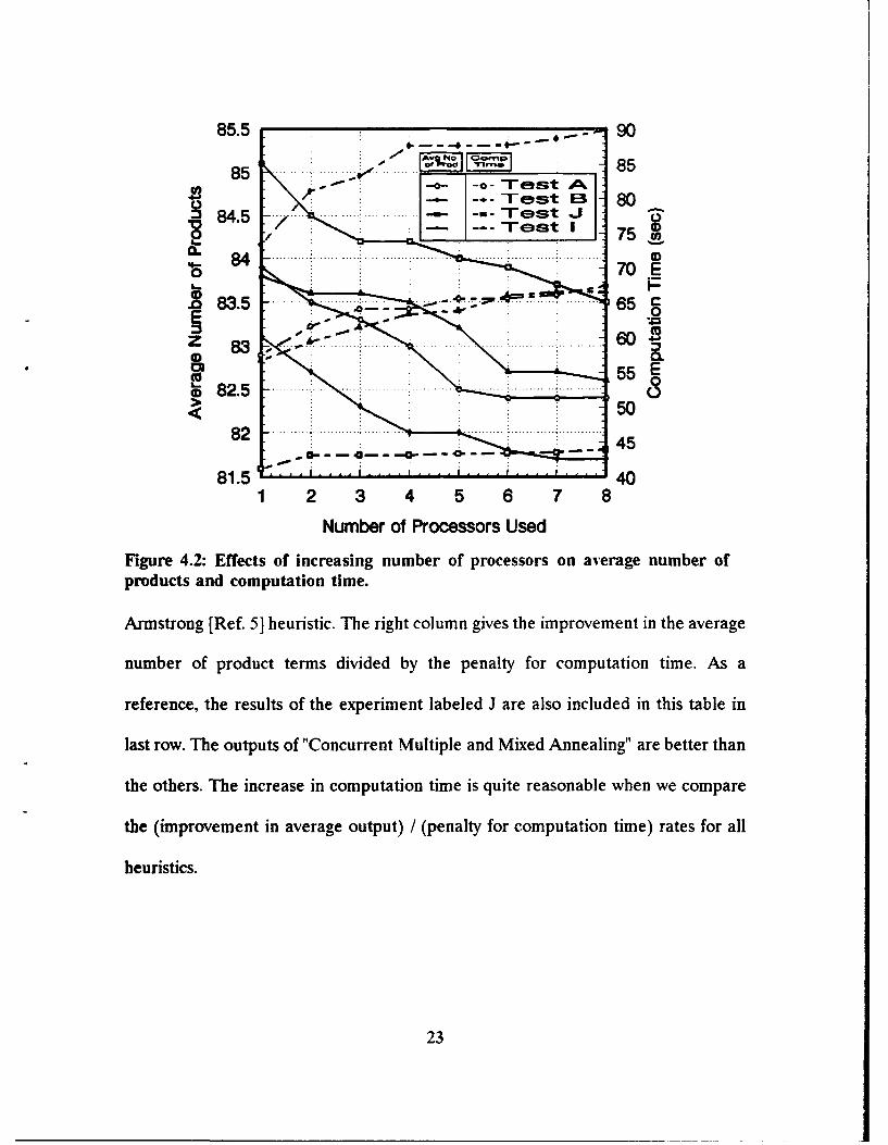
For some of the test results given in Table 2.3 (A, B, I, J), the effects of
increasing the number of processors are also investigated. In Fig. 4.2 we can see the
average number of product terms and the computation times, as a function of
number of processors used for concurrent multiple and mixed annealing. Figure 5.2
suggests that J and B are the best in taking advantage of having more processors.
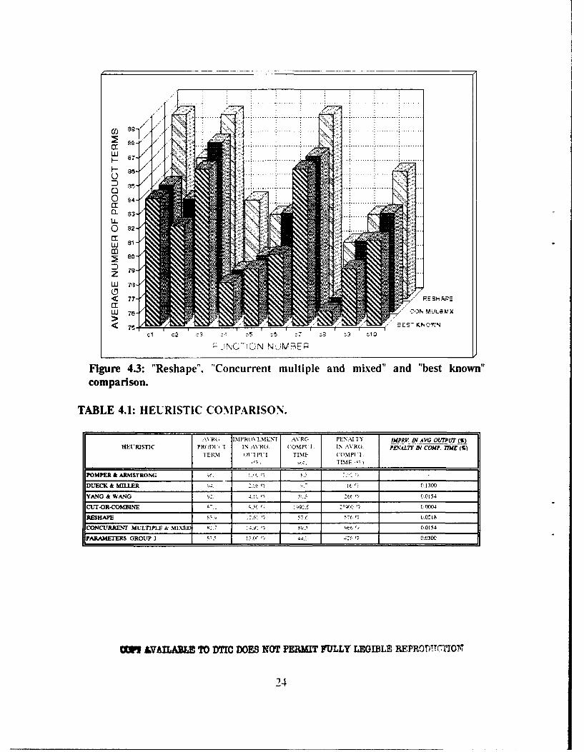
Fig. 4.3 shows the comparison between the regular Reshape and Concurrent
Multiple and Mixed Annealing for all the functions (C1,..,C1O). This figure also
includes the best results known. For five out of the ten cases, Concurrent Multiple
and Mixed Annealing does nearly as well as the best known results. Notice that
Reshape is significantly worse for the same functions. In all cases, Concurrent
Multiple and Mixed Annealing does better than Reshape.
In Table 4.1 below, the comparison of seven heuristics are given. To be able
to get a fair comparison, all the heuristics are compared with the Pomper &
22
85.5 9A'o O~mp 8
.85 . .. est A.S845
0 __ -in- Test EJ 80... .. .. -a T e t I- -_s 75
S84.70
700
83.5 .
* 82.5 05
.. .458 1 5 . . . . ' . . . .......... .. . . . . . .. . . . . . .. .. ... .. ....
1 2 3 4 5 6 7 8
Number of Processors Used
Figure 4.2: Effects of increasing number of processors on average number of
products and computation time.
Armstrong [Ref. 5] heuristic. The right column gives the improvement in the average
number of product terms divided by the penalty for computation time. As a
reference, the results of the experiment labeled J are also included in this table in
last row. The outputs of "Concurrent Multiple and Mixed Annealing" are better than
the others. The increase in computation time is quite reasonable when we compare
the (improvement in average output) I (penalty for computation time) rates for all
heuristics.
23
... ... ...
7z
FE fA
2-Nh;NNME
Figre 4.3:......... .Resape" "Concurrent multiple. an......nd "bstknwncomparsn
TABLE... 4.1 HEURISTIC. COMPARISO...N.-----.....
AN & a- G 83- ! ..........
0 824

V. CONCLUSIONS
The results and analysis of the tests show significant promise for the
Concurrent Multiple and Mixed Simulated Annealing. New approaches to Cut-or-
Combine and Reshape heuristics provided better performance than each heuristic
alone.
Mixing two moves, Cut-or-Combine and Reshape, in the same simulated
annealing experiment gave interesting results. For example, the mixing of a small
number of Cut-or-Combine moves (4%) with Reshape moves (96%) allows a
minimal solution to be found for a special function, which would be impossible if
100% of the moves were Reshape. The benefit of mixing moves was also shown by
our experiments on sets of functions where there were a low average number of
product terms (e.g. B and D in Fig. 4.1).
In addition to mixing two different moves, the multiple paths approach for a
simulated annealing experiment provided an additional benefit. Performing
simulated annealing experiments on a set of ten functions using eight different paths
gave better outputs in terms of number of product terms. This experiment yields
82.4 product terms versus 84.2, the expected number for one experiment. However,
this reduction had a cost, a large increase in time, 470.5 seconds for the better result
versus 58.0 seconds for the worse.
25

The solution to the large computation time for the multiple path approach was
to run multiple experiments concurrently on independent processors. This improved
the computation time considerably. With eight processors, there is the prospect of
a speedup of 8 over a single processor sequentially performing 8 experiments. The
speedups were found on the order of 7, indicating a diversity in computation times
over the 8 experiments (speedups of 8 are achievable only if all experiments require
identical computation time.)
Finally, the average number of product terms produced by each of 12
experiments are compared with the average number of product terms associated with
the best known results. For all experiments, a best result for each function is
achieved; the average of these represents the best known realization. The 12
experiments produced, out of approximately 81.1 product terms, a value higher by
between 0.5 and 5.9 than this best value.
There is clear advantage in using multiple processors. But, it is also clear that
there is a point of diminishing returns in using multiple processors. Our experience
suggests that at the eight processors used here, we are beyond that point. However,
our results also suggests that this is a fruitful area of research.
26
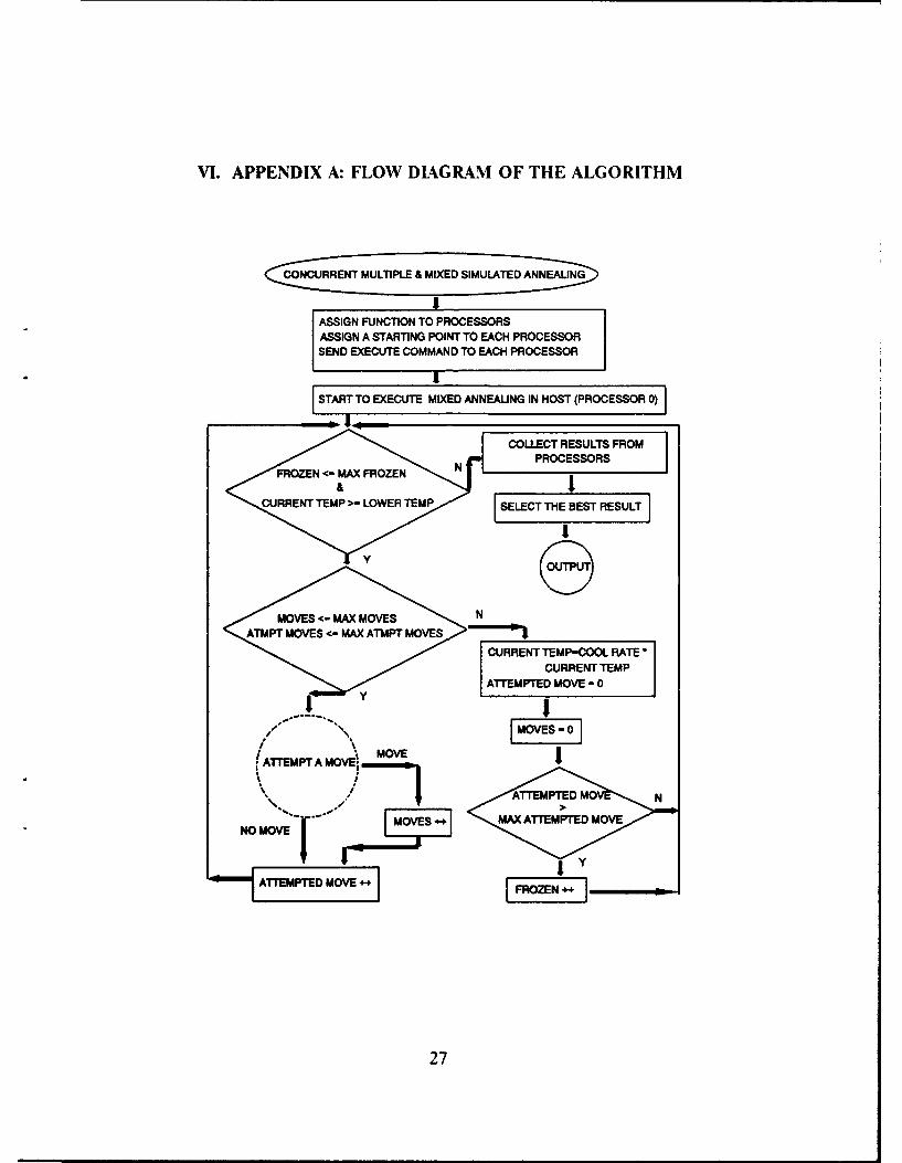
VI. APPENDIX A: FLOW DIAGRAM OF THE ALGORITHM
CONCURRENT MULTIPLE & MIXED SIMULATED ANNEAUNG
IASSIGN FUNCTION TO PROCESSORSASSIGN A STARTING POINT TO EACH PROCESSORSEND EXECUTE COMMAND TO EACH PROCESSOR
1
START TO EXECUTE MIXED ANNEAUNG IN HOST (PROCESSOR 0)
COLLECT RESULTS FROMPROCESSORS
N LL
MOVES - MAX MOVES N
CURRENT TEMP-COOL RATE
CURRENT TEMPATTEMPTED MOVE - 0
/y
/\
MATXEMPT A MOVEM MO
M !-NOMOE++
27
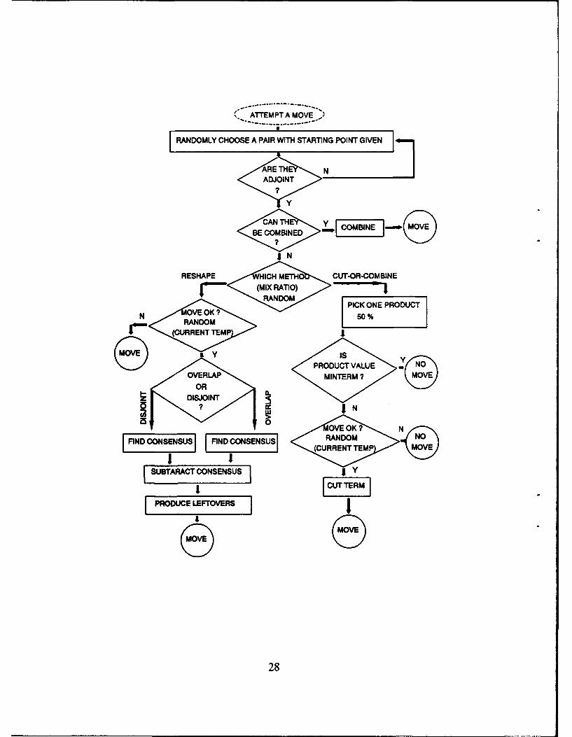
(*ATTEMPT A MOVE.,)
RANDOMLY CHOOSE A PAIR WITH STARTING POINT GIVEN
ADJOINT
<CAN
Y
BE COMBINED
I N
RESHAPE ICH METHO CUT-OR-COMBINE
fo-- (MIX RATIO)RANDOM
PICK ONE PRODUCTN VE OK ? 50%'4- RANDOM
(CURRENT TEMP
MOV IsPRODUCTV VLE
OVERLAPMINTERM?
OVE OK ? NFý SýU ý ýSNURANDOM NO
(CURRENT TEMP MOVE
SUBTARC CONSENSUS I Y
I
28
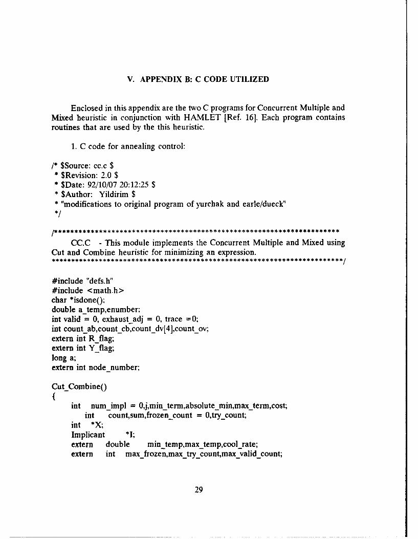
V. APPENDIX B: C CODE UTILIZED
Enclosed in this appendix are the two C programs for Concurrent Multiple andMixed heuristic in conjunction with HAMLET [Ref. 161. Each program containsroutines that are used by the this heuristic.
1. C code for annealing control:
/* $Source: cc.c $"* $Revision: 2.0 $"* $Date: 92/10/07 20:12:25 $"* $Author: Yildirim $"* "modifications to original program of yurchak and earle/dueck",/
CC.C - This module implements the Concurrent Multiple and Mixed usingCut and Combine heuristic for minimizing an expression.
#include "defs.h"#include <math.h>char *isdone0;double atemp,enumber;int valid = 0, exhaust adj = 0, trace =0;int count ab,count_cb,count_dv[4],count-ov;extern int R_flag;extern int Yflag;long a;extern int nodenumber;
CutCombineO
int num-impl = 0,j,minterm,absolutemin,maxterm,cost;int count,sum,frozen count = 0,try_count;
int *X;Implicant *I;extern double min temp,max-temp,cool_rate;extern int maxfrozen,max_try_count,max valid count;
29
long initc- pu.clocko:double tot cpu:FILE *fp:
/* Orpen output statistic file and initial clock counter for CPU time comparisons. ~fp = fopen("stats.out',"a"):.init cpu = clocko:if (TE finai CCj.1 != NULL)
dealloc -expr(&E final[CC]):HEUR = CC:dup~expr(&E -work.&E E orig):I* set parameters *if (R flag) I
if (max valid-count ==0)
max-valid-count =mintermso*MAXVALIDFACTORR;
if (max try count ==0)
maxftry-count =max -'alid count * MAX TRYFACTORR1;if (cool rate =0.0)
cool rate =COOLRATE R:
else Iif (max valid-count = 0)
max-valid-count =mintermso*MAXVALIDFACTORC;
if (max try_count ==0)
max_try count =max valid count * MAX TRYFACTORC;if (cool rate = 0.0)
cool-rate =COOLRATE C:
ik(E work. I= (Implicant* )realloc( E work. I,sizeof(Implicant) *MAXJ(TERM))-- NULL)
fatal("alloc~implicanto: out of mem ory\n");if (!vverify()) printf("we are in big trouble!\n");E -final[HEURJ.nterm =0:
E-final[HEUR].radix =E~orig.radix;
E-flnal[HEUR].nvar =E-orig.nvar;
E-final[HEURJ.I = NULL;resource -used(START);
count = 0;totý-cpu = 0.0;absolute-min = 1000000:a-teinp = max-temp;
30
printf(ttmax temp = (74-;.2f cool rate = 175.3f min temp = %5.3f\nmax frozen=%d "
max -temp,cool_rate.min -temp.max -frozen);printf("max try count = "4 d max-valid-count =7cn"
max try-count,max-%valid-count).
while ((a temp > mm itemp)& &(froze n-cou nt < max-frozen)){count cb = 0;foroj = 0; j < 4; j+ +) count dv[j] = 0;count-ov = 0;count ab = 0;valid = 0:max term = 0;min-term = 1000000:try count = 0:enumber = exp(-1.0'a temp):while((try count < max -try cou nt)& &(valid < max valid-count)){
pick a~pairo:if (a temp < 0.00)f
trace = 1:printf("nterm = 17(d\n",E-work.nterm);
if (E wýork.nterm< min-term)min-term = E-work.nterm;
if (E work.nterm> max-term)max term = E-work.nterm;
try-count+ +:
if (absolute -mmn > min term)absolute min = min _term;
if ((valid > = max -valid -count) && (min-term < max-term))frozen-count = 0.
elsefrozen-count+ +.
tot cpu =tot-cpu + (clock() - init~cpu)/1000.0;init~cpu =clocko:
printf(" %7.3f',a_temp):printf(" %3d %c3d 173d 9%6d",min_term,E-work.nterm,max-term,try__count);printf(" % 10.3f~n".tot_cpu/1000.0);a -temp = cool-rate * a-temp;Iresource used(STOP):.
31
dupeýxpr(&(E~final[CCj)&E-work):,dealloc~expr(& E-work);tot cpu = tot cpu + (clock() - init-cpu)/1000.O:printf('tcpu time used = 17(10.3f sec.\n",tot-cpu/1000.O);fprintf(fp,"%7,5.3f Vc4d *9%4d 17(10.3f node# %,d\n",cool-rate,E_orig.nterm,
absolute min,tot-cpu/1000.O,node-number);fclose(fp);
print map2()
:fnction:
-Print the Karnaugh map of E -work in its present state
register i~j;mnt X[MAX-VAR+2];int *V;
for (i=O; i < nvar; i++) X[iJ = 0;for (i=0; i < nvar:) I
V = eval(&E work,X);printf('% s%3d,7(c",X[i] == 0?" ":"",V[EVALI,V[HLVI?'.':'')X[i]+ +;for (;i < nvar:) I
if (X[i] > =radix){
X[i] 0;
X[i]+ +;
else{S= 0;
break;
printf("\n");
int vverify()
Verify that the integrity of the function is maintained
32
register Li:j
int X[MAX-VAR+2]:.int *V-.int first,second;
for (i=0; i < nvar: i++) X[i] =0;
for (1=0; i < nvar:) fV = eval(&E-work,X);first = V[EVAL];V = eval(&E_orig,X):second =V[EVAL];
if (first !=second) return(0);X[i] + +:for (:i < nvar:){
if (X~ij > =radix){
X[ij 0;i+ +:X[]]+ +;
else{S= 0:break.
return( 1;
find the sum (truncated) of all minterms in E work
int sumE-work()
register i~j;int X[MlAXVAR+21;int *V;int result;
for (1=0; i < nvar; i++) X[i] =0;
result = 0:for (i=0; i < fivar:){
V = eval(&E-work,X);
33
result = result + V[EVAL];X[iJ+ +;for (;i < nvar:) {
if (X[i] > = radix) {X[i] = 0;i++-.
X[i]+ +;}else {
i = 0;break;
}}
}return(result);
find the number of minterms in E work
int minterms0{
register ij;int X[MAXVAR+2];int *V;int result;
for (i=0; i < nvar: i+ +) X[i] = 0;result = 0;for (i=O; i < nvar;) {
V = eval(&Ework,X);result = result + (V[EVAL] > 1);X[i] + +;for (;i < nvar:) {
if (X[i] > = radix) {X[i] = 0;i+ +;
X[i]+ +;}else {
i= 0;break;
}
34
return(result);
find the sum (not truncated) of all minterms in E work
int oversum_E_work(
int i,j,resulttemp;
result = 0;for(i = 0; i < Ework.nterm; i++) {
temp = E-work.I[i].coeff;for (j = 0; j < nvar; j++ )
temp = temp * (E work.I[i].B[j].upper -
Ework.I[i].B[j].lower +1);result = result + temp;
}return(result);
35
2. C code for operation control:
/* $Source: reshape.c $"* $Revision: 2.0 $"* $Date: 92/10/07 20:12:25 $"* $Author: Yildirim $"* "modifications to original program of yurchak and earle/dueck"*/
This module controls the operations being conducted on the product terms. Italso controls the concurrency.
MultipleMixture (){extern long a;extern int nodenumber;extern char ifname[]:static char command[70]:static char processor[8] [6].res out[26];static int node_n.nodenn.dign,outn[8],minout n;static float outt[8],max_outt:static int max node=8;static char proc id[6]:static int ten_p[]= {1,10,100,1000};static float tenth_p[]= { 1.0,0.1,0.01,0.001 };
/* names of the workstations used in the system */strcpy(processor[ I ],"sun22");strcpy(processor[2],"sun6");strcpy(processor[3J,"sun8");strcpy(processor[4],"sun9");strcpy(processor[5 ],"sun 10");strcpy(processor[6],"sun 1I"):strcpy(processor[7],"sun17");/* different seeds for each random number generator of the processors */if(node number= = 7) {a=101301;}if(node number= =6) { a= 111001;}if(node number= =5) {a= 109001;}if(node number= =4) {a= 100701;}if(node number= =3) {a= 100501;}if(node number= =2) {a= 100301;}if(node-number= = 1) {a= 101001;}
36

if(node-number==0) {a= 100001:
for(node -n=l:node-n < max-nude ;node_n++){strcpy(proc id.processor[node n]):sprintf(command, "rsh 7(s 'cd node'7d I annea12 -Y%d %s»> hoho%d '&
,proc-id,node-n, node-n. if-name~node_n):system (command):
Rkflag+ +Y~flag--;,CutCombineo;if(node-number==0) I
fprintf(stderr," RESU LTS\n");min _out n =9999,max-out-t= LO:for(node_n=0:node-n <= (max-node-1);node n++)fstrncpy(res~out~isdone(node n),23);printf("\n result: 17es".res out)-.for(dig_n=0:di~gn<4:dig~n++){
ou t-n [nod e~n I= ou t~n [nod e~n] + (res Out[dig n]-'O')*ten~p[3-dig_ýj]* (res-out[dig_
if(out-n[node~n] < min out-n) min_out-n =out n[node n];printf("\n min out: %4d",min-out-n);for(dig_n=7:dig_n<11:dig~n++){
out-t~node~n] = out t[node n] + (res-out[dign]-'O') *ten~p[ 1O-dig~n]*(res~out[dig n]!='*)
for(dig_ýn=12;dig n< 15.dig n+ +){out -t[node~n = out t[node n + (res-out[dig~n]-'O') *tenth~p[dig~n-.11];
if(out-t[node~n] > max outt) max out-t= out t[node n];printf("\n max time= %4.3f',max-outt);
fprintf(stderr,'ALL DONEWn);
return;
37
Check if the processor finished its assignment
char *isdone(s no)int s-no;
static int iWonejr out,chn;static char ssn[20];char path name[19],ch out[26];FILE *jfp;done=O;sprintf(path_name,". ../node %d/stats. out", s no);while(done = = 0) fifp =fopen(path -name, 'r");i=fgetc(ifp);
while (i !=EOF){if (i == 'e){
done =1;
i=fgetc(ifp);I
fclose(ifp);
ifp=fopen(path_name, "tr")i= fgetc(ifp);
while(i !=EOF){
for(chn=0:chn<26;chn+ +){ch-out[chnl = fgetc(ifp);
ch -out[26] =NULL;break;
i= fgetc(ifp);
fclose(ifp);fprintf(stderr,"node %d done\n",s no);strcpy(ssn,ch_out);return(ssn);
38
Select to conduct reshape algorithm
#include ttdefs.h"int valid;extern int count -ab,count -cb,cou n t-ov,count dv[4], exhaust adj, trace;extern double enumber;exter n t. R_flag;extern long a;
pick a-pair()
nt, success,temp1,temp2,nterm,j,count~i;double d -randomo;success = 0;count = 0;while ((success 0) && (count < 100))
{ep admE-wr~tr)tempi = random(E work.nterm)-.
while (temp 1= temp2)f
temp2 = random (E-work. nterm);I
if ((templ < 0) II(temp 1 > = E -work.nterm) I(temp2 < 0) II(temp2 > = E -work.nterm)){
printf("alarm!! %d %Xd\n",temp 1,temp2);
if (IsAdj(& E work. I[templ ],&E-work. I[temp2]))f
if(trace)
printf("%d adji =",templ);Printlmp(&E work. I[temp II);printf("%d ad-dr = %d adj2 =",temp2,&E work. I[temp2]);Printxnip(&E-work. I[temp2]);
if (combine(& E-work. I[templ1 ],&E-work. I[temp2]) < 0)
c-subtract(temp2);
success =I
39
else
counlt+ +:
return(O);
subroutine to test for adjacency
IsAdj(impl,iinp2)Iniplicant *iflpl,*fimp 2;
int used,v index,bprime,aprime;
used =0;
for (v index = 0: v index < nvar;)
if (((*impl1).B[v_index]. lower) >((imp2).B[v_index].Ilower))
aprime = ((*imp 1 ).B[v~index].lower);
else
aprime = ((*imp2). B[v~index]. lower);
if (((*impl1).B[v_index]. upper) <=((*jmp2).B[v_index].upper))
bprime =((*imp 1). B [v index], upper);
else
bprime =((*jlnp2).B[v-index].upper);
if (bpriine > = aprime)
v-index+ +;
else if ((aprime == (bprime + 1)) && (used !=1))
40

Iv index+ +;used = 1:}
else{v index = nvar + 5;}
return(vjindex = =nvar);}
subroutine to select random numbers between 0 and nterm
double d_random ({
a = (a*125)%2796203;return((double)a/2796203);
}
subroutine to select random numbers between 0 and nterm
random (nterm)int nterm;{double d randomo;
return((int)(d-random(*nterm));}
A subroutine to combine two product terms if possible and torandomly chose one of the product terms to be randomly divided.
combine(impl,imp2)Implicant *impl,*imp2;
{int p-index,s index,combcountbmax,amin,c-varj,excess,cost;double dcost;extern double a-temp;
cost = 0;if (random(25)-1 = =0)
41
Rflag=O:.else
R-flag = 1;if (IsAbsorb(impl~imp2))
fcost--;
if (trace)printf("inabsorb 1\n');
count-ab ++:valid+ +;
else if (IsAbsorb (imp2, impl1))
cost--;if (trace)
printf("inabsorb2\n");(*impl).coeff = (*imp2).coeff;
for (j=O; j< nvar: j++)(*m{ ) j.lwr=( m2.BJ.lwr(*impl).B[jJ lower = (*imp2).B[j].lower;
count ab+ +;valid+ +;I
else if (IsOverlap(impl,imp2))f
count ov+ +;if (trace)
printf("inoverlap\n");(*mp1).coeff = (*imnp1).coff + (*imp2).coff;if((*mp1).coeff > = radix)
excess= (*imp1).coeff-(radix- );(*impl).coff = radix-I;
cost--;valid+ +;
else if (IsConibine(impl,inp2))
count cb+ +;if (trace)
42

printf("incombine\n't );for 0j=0; j< fivar; j+ +)
Iamin = ((* imp2)) B[j ].lower);
else
amin = ((*imp1). B[j]. lower);
if (((*imp 1).B[j].upper) <= ((*imp2).B[j].upper))
bmax = ((*imp2).B[j].upper);
else
bmax = ((*imp1). B [j]. upper);
(*imp1). B[j]. lower =amnin;
(*imnpI).B[jJ upper =bmax;
cost--;valid + +;
else if (R flag) fcost = ReshapeCost(impl,imp2);if (trace)
printfQ'cost = %d\n",cost);if (cost < 1)
dcost = 0.05;else
dcost = (double) cost;enumber = exp(-dcost/a-temp);if (d random() < enumber) f
count dv[cost] = count dv[cost] +1;
if (trace)printf("Reshape\n");
Reshape(impl ,imp2);valid + +;
else if (d random() < enumber){
43
if (random(3) - 1 0)divide(imp 1):
elsedivide(imp2'):-
cost+ +;valid + +;
return(cost);
Subroutine to determine if combinable
IsCombine(imp 1,iinp2)Implicant *imp1,*imp2 ;
int v -index,bpruine. aprime,bmax,amin,c-var;int used = 0;
for (v _index = 0; v-index < nvar;)fif (((*imp 1).B[v_index]. lower) >
((imp2).Blv_index]. lower))
aprime = ((*imp 1 ). B[v~index]. lower);
else
aprime = ((* ip2). B[vmindexI. lower);
if (((*imp1). Bjv_index].upper) <=((*ilnp2).B[v-index].upper))
bprime = ((*imp 1 ).B[v-index].upper);
else
bprime = ((*imp2).B[v~index].upper);
if ((((*imp1).B[v_index]. lower) = =((* imp2). B[v~indexl.lower))&&(((*imp 1).B1[v_index].upper) = = ((*ixmp2). B[vindex].upp~er))&&
v-index+ +;
44

else if ((aprime == (bprime + 1)) && (used !=1))fv index+ +:used = 1:
else
v index = nvar + 5;
return(v index = =nvar);
Subroutine to determine if complete overlap occurs
IsOverlap(impl,imp2)Implicant *impl,*imp2;
int v-index;for (v index = 0: v index < nvar:)
Iif ((((*imp 1). B[v_index]. lower) == ((*imp2). B[v~index].lower))&&
(((*imp 1). B[v_index].upper) = (*p2). B[vindex].upper)))fv-index+ +;
else
v-index = nvar + 5;
return(v index = = nvar);
Subroutine to do a simple divide on an implicant by variable
cut(imp,cvar,b -cut)Implicant *imfp;int c-var,b-cut;
45

int old_up:if (trace) I
printf("in cut Implicant in");Printlmp(imp),
Iold up = (* imp). B[c-var]. upper;(*imp). B[c varJ. upper =b-cut;add_implicant(imp);b-cut+ +;E-work. I[E-work. nterm -I]. B[c var]. lower = b-cut;E-Work.I[E-work.nterm-1l.B[c-var].upper = old_up;if (trace) f
printf("in cut Part 1 )
Printlmp(imp);printf('t in cut Part 2 )
Printlmp(&E-work.I[E-work.nterm-1]);
Subroutine to do a simple divide on an implicant by coefficient
cutcoeff(imp,c_cut -lowsc-cut-high)Implicant * imp:int c-cut-low.c-cut_high;
int old_up,p_index,j;(*imlp).coeff = c-cut-low;
if (trace)
printf("cut -coef -bef'):Printlmp(imp);
add implicant(imp);E-WOrk.I[Ework.nterm-1].coeff =c-cut-high;
if (trace)
printf("cut-coef-af');Printhnp(imp);
return(O):
46

Subroutine to randomly divide an implicant
divide(d imp)Implicant *d_imp;
fint v-index, i, total-cuts, r-cut, c-count,c-cut-low,c-cut-high;int k, kprime, j, listl[100], list2[100];total-cuts = 0;for(vjindex = 0; v index < nvar; v-index+ +)
fj = (*d imnp). B[v_index]. upper-(* dimp).B[v-index].Ilower;total-cuts = total-cuts + i;
Iif ((*d imp).coeff = = radix - 1)
for (k= 1; k<radix; k+ +)
if (k>(*d imp).coeff - k)
kprime = k;
else
kprime = ((*d imp).coeff - k);
for (j= kp,-ime; j <radix; j ++){it~]=klistl[i] = k;
c-count =ii
else
ccount = (*d imp).coeff,'2;
total-cuts = c-count + total-cuts;if (total-cuts ! = 0)
47
if (trace)
printf("INDIVIDE");Printlmp(d imp):
r-cut = random (total-cuts) + 1;
if (((*d imp).coeff = = radix- 1)&&(r cut <= c-count))
c-cut-low =listl[r cut]:c cut high =list'2[r cut]-.cutcoeff(d~imp,c-cut-low,c-cut-high);
else if (r~cut < (*d~imp).coeff)
c-cut-low =r-cut:
c-cut-high =(*d imp).coeff - r-cut;cutcoeff(d~imp,c-cut-low,c-cut-high);
else
r-cut = r-cut - (c-count);= 0;
while (((*d imp). B[i]. upper - (*d imp).B[i].lower) < r-cut)
r-cut = r-cut - ((* d imp). B[i]. upper - (*d~inp). B[i ].lower);
i+}
r-cut =(d imp). B[i]. lower + (r cut-I);cut(d imp, i,r cut);
return (0);
Subroutine to determine if one implicant can absorb another
IsAbsorb(impl1,imp2)Iniplicant *imp1,*ip2;
int v-index:V index = 0;if((*mpl).coeff == (radix - 1))
48
for (v index = 0; v index < nvar:)Iif ((((*impl1).Bfv_index]. lower) <= ((* imp2). B [vindex].Ilower))&&
(((*imp I). B3[vjindexj.upper) > =((*inip2).B[vindex]. upper))){v-index+ +;
else{v index =nvar + 5; }
return(v index = nvar);
Printlmp(I)Iniplicant *I;
{ int i;printf(" + %d"i,(*I).coeff);for (0 = 0; i < nvar; i ++)
{printf(H*x94 !d(9c d,%d)",i + 1,(*I1).B[i]. lower,(* I).B[i].upper);
printf("\n");
49
LIST OF REFERENCES
1. K. C. Smith, "The prospect for multivalued logic: a technology andapplication view, " IEEE Trans. Computers, Dec. 1981, pp. 619-632.
2. S. L. Hurst, "Multiple-valued logic - its status and its future," IEEE Trans.Computers, Vol C-33, Dec. 1984, pp. 1160-1179.
3. H. G. Kerkhoff "Theory and design of multiple-valued logic CCD's," inComputer Science and Multiple-J/ahled Logic (ed. D. C. Rine),NorthHolland,New York, 1984, pp. 502-537.
4. J. Butler and H. G. Kerkhoff "Multiple-valued CCD circuits," IEEE Computer,March 1988, pp. 58-69.
5. G. Pomper and J. A. Armstrong, "Representation of multivalued functionsusing the direct cover method," IEEE Trans. Comp., Sep. 1981, pp. 674-679.
6. P. W. Besslich, "Heuristic minimization of MVL functions: a direct coverapproach," IEEE Trans. Comp., Vol C-35, Feb. 1986, pp. 134-144.
7. G. W. Dueck and D. Miller, "A direct cover MVL minimization using thetruncated sum," Proc. of 17th Inul. Symp. on MVL, 1987, pp. 221-226.
8. G. W. Dueck, Algorithms for the minimizations of binary and multiple-valuedlogic functions, Ph. D. Dissertation, Department of Computer Science,University of Manitoba, Winnipeg, MB, 1988
9. P. Tirumalai and J. T. Butler, "Analysis of minimization algorithms formultiple-valued PLA's," Proc. of 18th Intl. Svmp. on MVL, 1988, pp. 226-236.
10. E. E. Witte, R. D. Chamberlain, M. A. Franklin,"Parallel Simulated Annealingusing speculative computation" IEEE Trans. Parallel and Distributed Systems,Vol 2-4,1991, pp. 483-494.
11. G. W. Dueck, R. C. Earle, P. Tirumalai, J. T. Butler, "Multiple-valuedprogrammable logic array minimization by simulated annealing" Proc. of 22ndIntl. Symp. On MVL, 1992, pp. 66-74.
50
12. S. Kirkpatrick, C. D. Gellat, Jr., and M. P. Vecchi, "Optimization by simulatedannealing" Science, vol. 220, No. 4598, 13 May 1983, pp. 671-680.
13. G. W. Dueck, R. C. Earle. P. Tirumalai, J. T. Butler, "Multiple-valuedprogrammable logic array minimization by simulated annealing" NavalPostgraduate School Technical Report NPS-EC-92-004, Feb 1992.
14. C. Yang and Y. M. Wang, "A neighborhood decoupling algorithm fortruncated sum minimization," Proceedings of the 1990 International Symposiumon Multiple- Valued Logic, May 1990, pp. 153-160.
15. C. Yang and 0. Oral, "Experiences of parallel processing with direct coveralgorithms for multiple-valued logic minimization," Proceedings of the 1992International Symposium on Multiple- Vahled Logic, May 1992, pp. 75-82.
16. J. M. Yurchak and J. T. Butler, "HAMLET - An expression compiler/optimizerfor the implementation of heuristics to minimize multiple-valuedprogrammable logic arrays" Proceedings of the 1990 International Symposium onMultiple-Valued Logic, May 1990, pp. 144-152.
17. J. M. Yurchak and J. T. Butler, "HAMLET user reference manual," NavalPostgraduate School Technical Report NPS-6290-015, July 1990.
51
INITIAL DISTRIBUTION LIST
No. of Copies
1. Defense Technical Information Center 2Cameron stationAlexandria, VA 22304-6145
2. Library, Code 52 2Naval Postgraduate SchoolMonterey, CA 93943-5002
3. Chairman, Code EC 1Department of Electrical andComputer EngineeringNaval Postgraduate SchoolMonterey, CA 93943-5000
4. Professor Jon T. Butler, Code EC/Bu 1Department of Electrical andComputer EngineeringNaval Postgraduate SchoolMonterey, CA 93943-5000
5. Dr. George Abraham, Code 1005 1Office of Research and TechnologyNaval Research Laboratories4555 Overlook Ave., N.W.Washington, DC 20375
6. Dr. Robert Williams 1Naval Air Development Center, Code 5005Warminister, PA 18974-5000
7. Dr. James Gault 1U.S. Army Research OfficeP.O. Box 12211Research Triangle Park, NC 27709
52
8. Dr. Andre van Tilborg 1Office of Naval Research, Code 1133800 N. Quincy Str.Arlington, VA 22217-5000
9. Dr. Clifford LauOffice of Naval Research1030 E. Green Str.Pasadena, CA 91106-2485
10. Deniz Kuvvetleri KomutanligiPersonel Egitim Daire Ba§kanligiAnkara, TURKEY
11. Deniz Harp Okulu KomutanligiTuzla istanbul, TURKEY
12. G61ciik Tersanesi KomutanligiG61ciik Kocaeli, TURKEY
13. Ta§kizak Tersanesi KomutanligiKasinpa§a Istanbul, TURKEY
53