Embed Size (px)
Citation preview
AD-A275 055
NAVAL POSTGRADUATE SCHOOLMonterey, California
I.
THESIS
DEVELOPMENT OF COST ESTIMATING RELATIONSHIPSFOR MISSILE ENGINEERING MANUFACTURING DEVELOPMENT
(EMD) COSTS AND WARSHIP FUEL CONSUMPTION
by
Sandr, A. Williams
September, 1993
Thesis Advisor: Dan C. Boger
Approved for public release; distribution is unlimited.
94-02!573
41
REPORT DOCUMENTATION PAGE Form Approved OMB Np. 0704
Public reporting burden for this collection of information is estimated to average I hour per response, including the time for reviewing instruction,seam. hing existing data sources, gathering and maintaining the data needed, and completing and reviewing the collection of information. Sendcommetlls regarding this burden estimati or any other aspect of this collection of informatlon, including suggestions for reducing this burden, toWuhinion headquarters Services, Directorate for Information Operations and Reports, 1215 Jefferson Davis Highway, Suite 1204, Arling.i'n, VA22202.4302, and to the Office of Management and Budget, Paperwork Reduction Project (0704-018) Washington DC 20503.
1. AGENCY USE ONLY "2. REPORT DATE 3. REPORT TYPE AND DATES COVERED
I September 1993 Master's Thesis
4. TITLE AND SUBTITLE DEVELOPMENT OF COST ESTIMATING 5. FUNDING NUMBERSRELATIONSHIPS FOR MISSILE ENGINEERINGMANUFACTURING DEVELOPMENT (EMD) COSTS ANDWARSHIP FUEL CONSUMPTION
6. AUTHOR(S) Sandra A. Williams7. PERFORMING ORGANIZATION NAME(S) AND ADDRESS(ES) 8. PERFORMING
Naval Postgraduate School ORGANIZATIONMonterey CA 93943.,5000 REPORT NUMBER
9. SPONSORING/MONITORING AGENCY NAME(S) AND ADDRUSS(ES) 10. SPONSORINU/MONITORINGAGENCY REPORTNUMBER
11. SUPPLEMENTARY NOTES The views expressed in this thesis are those of the author and do notreflect the official policy or position of the Department of Defense or the U.S. Government.12a. DISTRIBUTION/AVAILABILITY STATEMENT I12b. DISTRIBUTION CODE
Approved for public release; distribution is unlimited.13, ABSTRACT
The purpose of this thesis Ij to develop estimating relationships for missile Engineering and MxnufacturingDevelopment (EMD) costs and warship fel consumption to aid the Naval Center for Cost Analysis (NCA) inperforming independent cost estimates for new weapons programs, Standard factors, which represent the percent thateach colt element is typically allocated from the program's total funding, are currently used to predict whether missileEMD costs are "roughly right," For fuel consumption, estimating relationships have only been developed for existingindividual ship types, None have been developed which use pooled ship types to estimate fuel consumption of new shiptypes, Regression analysis was used to develop estimating relationships based on physical and technical characteristics.
The cost estimating relationships (CERs) developed to predict missile EMD costs explained only about 34 percent ofthe variance, Due to the low explanatory power, no significant physical or technical factors could be determined. Eventhough the results are not statistically significant, the associated coefficients of variation are lower than the standardfactor coefficients of variation.
An estimating relationship with high explanatory power was developed to predict fuel consumption for newwarships. Three significant physical and performance factors were determined: steaming hours, agc and full loaddisplacement. For new ship types, steaming hours and full load displacement are the significant factors,
14. SUBJECT TERMS Cost Estimating Relationships, Missile Engineering 15. NUMBER OFManufacturing Development (EMD) Costs, Warship Fuel Consumption. PAGES 104
16. PRICE CODE
17. SECURITY CLASSIFI- 18, SECURITY CLASSIFI- 19, SECURITY CLASSIFI- 20. LIMITATION OFCATION OF REPORT CATION OF THIS PAGE CATION OF ABSTRACTUnclassified Unclassified ABSTRACT UL
Unclassified4SN 7340-01-230-5500 standard Fom29 (Rev, 2-J
Prescribed by ANSI Std 239-19
Approved for public release; distribution is unlimited.
DEVELOPMENT OF COST ESTIMATING RELATIONSHIPSFOR MISSILE ENGINEERING MANUFACTURING DEVELOPMENT
(EMD) COSTS AND WARSHIP FUEL CONSUMPTION
by
Sandra A. Williams
Lieutenant, United States Navy
B.S., Loma Linda University, 1983
Submitted in partial fulfillment
of the requirements for the degree of
MASTER OF SCIENCE IN OPERATIONS RESEARCH
from the
NAVAL POSTGRADUATE SCHOOL
September, 1993
Author: 514-& ý% 41 Lod6 &CiLvc4.eSandra A. Williams
Approved by: _ _ _ _ _ _ _ _ _ _ _ _ __4.-
Dan C, Bo7er, T {s Advsor
Mica Sjerei on d eader
Peter Purdue, Chairman
Department of Operations Research
ABSTRACT
The purpose of this thesis is to develop estimating relationships for missile Engineering and
Manufacturing Development (EMD) costs and warship fuel consumption to aid the Naval Center
for Cost Analysis (NCA) in performing independent cost estimates for new weapons programs.
Standard factors, which represent the percent that each cost element is typically allocated from
the program's total funding, are currently used to predict whether missile EMD costs are "roughly
right." For fuel consumption, estimating relationships have only been developed for existing
individual ship types. None have been developed which use pooled ship types to estimate fuel
consumption of new ship types, Regression analysis was used to develop estimating relationships
based on physical and technical characteristics.
The cost estimating relationships (CERs) developed to predict missile EMD costs explained
only about 34 percent of the variance. Due to the low explanatory power, no significant physical
or technical factors could be determined. Even though the results are not statistically significant,
the associated coefficients of variation are lower than the standard factor coefficients of variation.
An estimating relationship with high explanatory power was developed to predict fuel
consumption for new warships. Three significant physical and performance factors were
determined: steaming hours, age and full load displacement. For new ship types, steaming hours
and full load displacement are the significant factors. I Accesicn For
NTIS CRA&I MDIIC I ABUidoinoulOi(cod L.J
DTO IJM'~ LIN3P1~CED 5 .1By .. ,..... ... .. -----------
13y _ .... ..... . .................... ...... .... .Dit,l ib~itiori I
Avwilability Cods -Avail aid I or
Dist Spucial
ill I
DISCLAIMER
The reader is cautioned that computer programs developed in this research may not have
been exercised for all cases of interest, While every effort has been made, within the time
available, to ensure that the programs are free of computational and logic errors, they cannot be
considered validated. Any application of these programs without additional verification is at the
risk of the user.
iv
TABLE OF CONTENTS
I. INTRODUCTION . . . . . . . . . . . . . . . . . . . I
A. THE PROBLEM . . . . . . . . . . . . . . . . . 1
B. PURPOSE . . . . . . . . . . . . . . . . . . 2
1. Missile EMD Costs .0** ** . . 3
2. Warship Fuel Consumption . ........... 3
C. OVERVIEW . . . . . . . . . . . . . . . . . . . 4
II. MISSILE EMD COSTS . . . . . . ....... . . 6
A. PROBLEM DESCRIPTION ............ 6
B. DESCRIPTION OF DATA . . . . . . . . . . . 7
1. Cost Data . . . .................. 8
2. Technical and Operational Data . ..... 9
C. DEVELOPMENT OF THE MODEL . . . . . . . . 9
1. Dependent Variables. ........ . . .... 10
a. Design Costs (DES) . . . . . ....... 10
b. Hardware Costs (HW) . .................. 10
c. Software Costs (SW) .I.................. 10
d. Support Costs (SUP) ......... .... .. .. 11
e. Miscellaneous Costs (MISC) ... ...... .. 11
f. Total Costs (TOT) ...... ....... 11
2. Independent Variables .... .............. 11
a. Missile Type (D1,D2,D3,D4) ............ 11
v
b. Launch Weight (LWT.. ... .......... 12
c. Range (RNG) ............ . . ........... 12
d. IOC . . . . . . . . . . . . . . . . . . 12
D. REGRESSION WITH INITIAL DATA SET .... 13
1. CER Development .. . ..... .. 13
a. Design costs ........... 14
b. Hardware Costs . . . . . . . . . ... . 15
c. Software Costs . . . . . . . ..... 15
d. Support Costs ...... .. . ........ . 15
e. Miscellaneous Costs . . . .. . . 15
f. Total Costs . . . . . . . . . . . . 15
2. Coefficient of Variation . . . .. . . .. 6
E. PROBLEMS WITH THE COST DATA. . . . .. . 18
F. REGRESSION WITH "CLEANER" DATA SET . . . 21
1. CER Development ..... ................ 22
a. Design Costs .... .................... 22
b. Hardware Costs . . . ................... 23
c. Software Costs .......... ........ .. 24
d. Support Costs ........... ........ .. 24
e. Miscellaneous Costs ......... ..... .. 25
f. Total Costs ....... ... . . . .. 25
2. Coefficient of Variation .... .......... .. 26
G. COMPARISON OF RESULTS ............ ............. 27
H. SUMMARY .............. .................... 28
III. WARSHIP FUEL CONSUMPTION ..... ............ 30
vi
A. PROBLEM DESCRIPTION ........ .............. .. 30
B. DESCRIPTION OF DATA ........ . . . . .. 31
1. OPTEMPO And Fuel Consumption Data 32
2. Physical and Performance Data ....... 32
3. Constructing the Initial Data Base 34
4. Exploring Properties of the Data ........ .. 35
a. What proportion of fuel is used
underway? . . . . . . . . . . . . . . . 36
b. Evaluate relationship between barrels of
fuel consumed underway and steaming hours
underway . . . . . . . . . . . . . . . . 36
c. Data Transformation .......... 38
5. Constructing the Regression Data Base . . 41
C. DEVELOPMENT OF THE MODEL . . . . . . . . 42
1. Average Steaming Hours Underway (ASHU) . . 42
2 . Age . . . . . . . . . . . . t 4. . . . .. . . 43
3. Full Load Displacement (DISPFL) . . . . . 43
4. Overall Length (LENOA) .... ........... .. 44
5. Beam .............. .................... .. 44
6. Draft . . . . .................. 44
7. Total Shaft Horsepower (TSHP) .. ...... .. 45
8. Speed. ........ . . . . . . . . . 45
D. RESULTS OF THE BASIC MODEL . . ............... 47
E. ALTERNATIVE SPECIFICATIONS . . ............... 49
1. Basic Model ... ......... ............. 50
2. Alternative 3: Delete SPEED . ............ 50
vii
3. Alternative 2: Delete TSHP ... ........ .. 50
4. Alternative 3: Delete SPEED, TSHP ........ 50
F. HETEROSCEDASTICITY . . . . ................... 53
i. Definition ............... ........... 53
2. Correction . . . . . . . . .... . . .............. 54
3. Results of the Corrected Model . . . . . . 56
G. ALTERNATIVE DATA STRUCTURES . . . . . . . . . 57
H. SUMMARY ... 58
IV. CONCLUSIONS AND RECOMMENDATIONS . . . . . . . . . 60
APPENDIX A .................. . . . 62
APPENDIX B . . . . . . . . . . . 65
APPENDIX C ........................... 67
APPENDIX D ........................................... 73
APPENDIX E ........................................... 74
APPENDIX F 75
APPENDIX G ........................................... 76
APPENDIX H ........................................... 77
viii
LIST OF REFERENCES ........... .................. 89
INITIAL DISTRIBUTION LIST ........ ............... 91
ix
EXECUTIVE SUMMARY
The purpose of the thesis is to develop estimating
relationships for missile Engineering and Manufacturing
Development (EMD) costs and warship fuel consumption for the
Naval Center for Cost Analysis (NCA). NCA performs
independent cost analyses on cost estimates submitted by
program managers of major weapons systems, using the
methodology most appropriate to the weapons program under
study, to ensure they are credible. To refine its current
cost estimation methods and techniques, NCA was interested in
developing new estimating relationships based on physical and
technical characteristics.
The goal of the first section is to develop estimating
relationships which predict the total EMD cost, or its element
costs, for new missile programs coming on-line based on
technical and operational parameters. Currently NCA uses
standard factors, which represent the percent that each
element is typically allocated from the program's total
funding, to judge whether funding for major acquisition
programs are "roughly right." A data base containing EMD
costs and technical and physical characteristics, such as
missile type, launch weight, range and initial operational
capability (IC), was created. A "best fit" regression was
performed. The results from the regression were used to
address the following questions:
x
* Are the developed cost estimating relationships (CERs)statistically significant? If so, what are thesignificant physical or technical factors that affectcost?
* If the result is not significant, is the CER coefficientof variation below that of the standard factors? If so,the developed CER may be a better predictor than thestandard factors.
The initial results were poor, so an attempt was made to
make the data "cleaner" by deleting dual observations and
observations which could not be matched to a particular
missile series. The results from the second regression were
also poor. The developed CERs explain, at the most, only
about 34 percent of the variance. No significant physical or
technical factors could be determined due to the low
explanatory power. Even though the results are not
statistically significant due to the low explanatory power,
the associated coefficients of variation are lower than the
standard factor coefficients of variation. This means that
these developed CERs may be better predictors than the
standard factors in use.
The goal of the second section is to develop an estimating
relationship to predict fuel consumption for new ships coming
on-line. Since fuel costs make up a large part of the
Operations and Support (O&S) cost, accurately predicting fuel
consumption is vital for the estimatior of that part of the
cost estimate. NCA was interested in developing an estimating
relationship that used physical and performance factors to
xi
estimate fuel consumption. This study (,f fuel consumption was
restricted to seven warship types. After a composite data
base was developed, linear regression was performed. The
results from the regression were used to address the following
questions:
0 Are the results significant? If so, what are thesignificant physical and performance factors that drivefuel consumption of warships?
Based on the results of the analysis, an estimating
relationship with a high explanatory power has been deve2oped
which predicts fuel consumption of warships. The significant
physical and performance factors are steaming hours, age and
full load displacement. For new ships, steaming hours and
full load displacement are the significant factors. The
estimating relationship should be of great help in predicting
fuel consumption for inclusion in the O&S cost estimate. It
is important that this CER only be used to predict fuel
consumption for ships whose characteristics are similar to
those in the data base.
xii
I. INTRODUCTION
A. THE PROBLEM
Cost analysts are always looking for ways to more
accurately predict future costs. Estimating costs for new
programs is extremely difficult. Due to the uncertainty of
the factors that impact cost, such as implementing new
technology in an existing system or developing an entirely new
system, a currently reliable cost estimating tool that does
not include these may not perform as well in the future.
One agency responsible for analyzing costs and preparing
cost estimates is the Naval Center for Cost Analysis (NCA).
The mission of NCA is "...to provide independent cost and
financial analyses to support the Secretary of the Navy."
[Ref. 1:p. 1] It independently analyzes cost estimates
submitted by program managers of major weapons systems to
ensure they are credible. Additional tasks include financial
analyses of defense contractors and economic analyses of
acquisition issues. [Ref. 1:p. 1]
When NCA is tasked with performing an independent cost
analysis, it establishes the program baseline and work
breakdown structure. These provide the foundation upon which
to build the analysis. NCA performs its own independent cost
estimate, using the methodology most appropriate to the
1
weapons program under study. The program manager's cost
estimate is compared to NCA's estimate. Any differences are
reconciled, if possible, and uncertainty and risk/sensitivity
analysis is performed. The bottom line of the analysis is to
answer the question, "Is the program manager's estimate
reasonable?" [Ref. 2:p. 11]
The commodities for which NCA provides independent cost
analyses are aircraft, Automated Information Systems (AIS),
electronics, missiles, ships, and torpedoes. NCA was
interested in developing new Cost Estimating Relationships
(CERs) based on physical and technical characteristics in
these six areas so that it could refine its current cost
estimation methods and techniques. [Ref. 3:p. .1 Two initial
areas of study were identified, missile EMD costs and warship
fuel consumption.
B. PURPOSE
The purpose of the thesis is to develcp estimating
relationships for missile Engineering and Manufacturing
Development (EMD) costs and warship fuel consumption.
Specific physical and technical characteristics will be
identified, as appropriate, for inclusion in the models. The
goal is to develop reliable estimating tools that can be used
by NCA in future independent cost analyses.
2
1. Minsile END Costs
In November 1992, a Standard Cost Factors Handbook was
published by NCA to provide "rules of thumb" for senior
management to use in judging whether acquisition cost
estimates were "in the ballpark." These "rules of thumb" were
developed for Engineering and Manufacturing Development (EMD)
and Procurement costs for six commodities: aircraft, AIS,
electronics, missiles, ships, and torpedoes. [Ref. 4:p. iii]
One area, EMD costE for missiles, was identified as a
potential area for further study. NCA was interested in
determining whether a more reliable cost estimating tool which
incorporated technical and physical characteristics could be
developed. A data set containing EMD costs and technical and
physical characteristics was created. A "best fit" regression
was performed on the data. The results from the regression
were used to answer the following questions:
* What are the significant physical or technical factorsthat affect cost?
0 Are the results significant? I.e., is the developed CERstatistically significant?
* If the results are not significant, is the CER coefficientof variation below that of the standard factors? If so,the developed CER may be a better predictor than thestandard factors.
2. Warship Fuel Consumption
Another area of interest was estimating fuel
consumption for new ships coming on-line. Since fuel costs
3
make up a large part of the Operations and Support (O&S) cost,
accurately predicting fuel consumption is vital for the
estimation of that part of the cost estimate. NCA was
interested in developing an estimating relationship that used
physical and performance factors to estimate fuel consumption.
Again, this would provide NCA analysts with another tool to
estimate fuel consumption of new ship types or classes. This
study of fuel consumption was restricted to seven warship
types. After a composite data base was developed, linear
regression was performed. The results from the regression
were used to answer the following questions:
0 What are the mignificant physical and performance factorsthat drive fuel consumption of warships?
* Are the results significant?
C. OVERVZMW
The thesis is divided into two sections, missile EMD costs
and warship fuel consumption. Missile EMD cost estimating
relationships are developed in Chapter II. Warship fuel
consumption estimating relationships are developed in Chapter
1II. Chapter IV contains the Conclusions and Recommendations.
Appendix A contains the initial data set of missile EMD costs,
while Appendix B contains the cleaner data set. Appendix C
contains the warship fuel consumption data. The next four
appendices contain statistical information on the excursions
4
run on the base model (Appendix D), Alternative 1 (Appendix
E), Alternative 2 (Appendix F), and Alternative 3 (Appendix
G). Appendix H contains statistical information on additional
excursions which deleted independent variables considered
critical to the model.
5
11. MISSILZ ]lD COSTS
A. PROBLEM DESCRIPTION
The goal of this chapter is to develop estimating
relationships which predict the total EMD cost, or its element
costs, for new missile programs coming on-line based on
technical and operational parameters. Currently NCA uses
standard factors, which are published in its Standard Cost
Factors Handbook, to judge whether funding for major
acquisition programs are "roughly right." A standard factor
is associated with each element of the program, for example,
design. These standard factors represent the percent that
each element is typically allocated from the program's total
funding. The problem is that these factors do not consider
technical and operational parameters, so they can never be
more than "roughly right." [Ref. 4:p. iii) The need for a
more accurate methodology became evident. Development of a
cost estimating relationship based on technical and
operational characteristic-s became a high priority. This
chapter will concentrate on developing a CER to predict
missile EMD costs.
During the selection process, Dr. Daniel Nussbaum,
Director of the Missile Division (NCA-4), provided much needed
guidance on which technical and operational characteristics to
6
include in the model. The technical and operational
characteristics were missile type, launch weight, and range.
Initial operational capability was added as a proxy for the
level of technology available. These four characteristics
shaped the initial model.
The cost data in the handbook was derived from several
sources, for example, contractor cost reports. Care was taken
to make the data consistwnt and comparable, but this proved to
be a daunting task. Costs from different sources conflicted.
For example, one source separately listed costs for the
software element, but a second did not, In another case, the
difference between the cost elements for dual observations of
the same missile was on the order of 400 percent. Despite
these problems, it was felt that the data should be explored
to see whether usable results could be developed. In a later
section, the problems with the data will be more fully
discussed and an attempt to derive "cleaner" data will be
explored.
D. DESCRIPTZON OF DATA
The regression model to be developed depends exclusively
on the data obtained. Two sources of data were identified.
The Standard Cost Factors Handbook contained missile EMD
costs. The U. S. Missile Data Book, 1993 contained the
technical and operational characteristics for the missiles
under study. The data from the two sources were combined t-
7
provide input to the regression model. The missile data is
shown in Appendix A. Since the data is cross-sectional, no
time-series complications are anticipated. However, use of
IOC as an independent variable may induce autocorrelation.
This will be checked via the Durbin-Watson statistic. There
may be a heteroscedasticity problem since the assumption of
constant error variance may be unreasonable.
1. Cost Data
The Standard Coat Factors Handbook contains cost data
for each of the five elements of the missile EMD phase,
standardized in FY 1989 dollars. The elements are design
(DES), hardware (HW), software (SW), support (SUP), and
miscellaneous (MISC) These five elements -are summed to
produce total cost (TOT). Twenty-eight observations are
reported. Eased on discussions with Dr. Nussbaum, it was
decided to delete five observations. Observations were
deleted if they were not missiles, if technical and
operational characteristics could not be found, or if they
were duplicate observations. For example, VIPER was deleted
because it was an underwater robotic vehicle system used in
mine countermeasures. [Ref. 5:p. 63) The ROLAND missile was
deleted because it was not a missile used by U. S. forces.
The SLAT was deleted because no technical or operational data
could be found. Finally, one set of STINGER and STINGER/POST
8
data was deleted in favor of another more, accurate data set.
This left 23 observations in the data set.
2. Technical and Operational Data
The following data was collected from the U.S.
Missile Data Book. 1993 for each missile studied:
* missile type
• launch weight
• range
* initial operational capability (IOC).
Based on expert knowledge within NCA's Missile
Division, missile type, launch weight, and range were chosen
as the variables most likely to have explanatory power. The
initial operational capability date was added to act as a
proxy for the level of technology available for inclusion into
the program. Details on these variables are provided below,
C. DEVELOPMENT OF THE MODEL
The basic objective was to develop a CER to predict
missile EMD costs using the data from the Standard Cost Factor
Hadok. The dependent variable is EMD cost. However, the
available observations [Ref. 4:pp. 37-39] contain not only
total EMD costs but individual element costs, such as design,
hardware, software, support, and miscellaneous. Therefore,
six CERs will be developed, if possible.
9
L MII IIII II IIIII
In developing a basic model for missile EMD costs, certain
a pr-orl expectations about the independent variables to be
included in the estimation equation shape the model:
ESdW Cost - f (missile type, launch weight, range, IOC)
It is assumed that the independent variables will provide
explanatory power for each dependent variable.
1. Dependent Variables
a. Design Costs (DRS)
Design costs consist of "the cost of the
engineering analysis required to transform a concept into
released drawings, engineering data, and final hardware."
[Ref.4:p. 891 The variable is measured in millions of FY 1989
dollars.
b. Hardware Comes (MW)
Hardware costs consist of "the vehicle which is the
primary means for delivering the destructive effect to the
target, including the capability to generate or receive
intelligence, to navigate and penetrate to the target area and
to detonate the warhead. It includes the propulsion system,
payload, airframe, reentry system, guidance and control
equipment, and command and launch equipment." [Ref. 4:p. 89)
The variable is measured in millions of FY 1989 dollars.
a. Software Costs (OW)
Software costs consist of "the effort required to
develop computer software for the weapon system which will
10
provide for operational, data analysis, simulation, and other
user requirements." (Ref. 4:p. 89) The variable is measured
in millions of FY 1989 dollars.
d. Support costs (SUP)
Support costs include applicable costs for system
engineering/program management, system test and evaluation,
data deliverables, special tooling and test equipment, and
integrated logistics support. [Ref. 4:pp. 89-90) The variable
is measured in millions of FY 1989 dollars.
*. Misaellaneous Comes (MISC)
Miscellaneous costs consist of all other costs that
do not fit into the above categories. (Ref. 4:p. 911 The
variable is measured in millions of FY 1989 dollars.
f. Total Costs (TOT)
The total cost is the sum of design, hardware,
software, support and miscellaneous costs. The variable is
measured in millions of FY 1989 dollars.
2. Independent Variables
a. Missile Type (D1,D2,D3,D4)
These four dummy variables represent the missile
type for each observation. Table I gives the complete codes
for each missile type. For example, an air-to-air missile
would be represented by Di equal to one and the other dummy
variables (D2, D3, D4) equal to zero.
1.
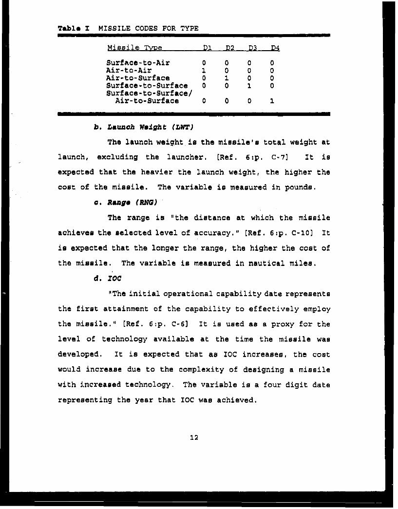
Table I MISSILE CODES FOR TYPE
Missile Tyve DL1 D2 D3 D4
Surface-to-Air 0 0 0 0Air-to-Air 1 0 0 0Air-to-Surface 0 1 0 0Surface-to-Surface 0 0 1 0Surface-to-Surface/
Air-to-Surface 0 0 0 1
b. Lsunach Weight (LWT)
The launch weight is the missile's total weight at
launch, excluding the launcher. [Ref. 6:p. C-7] It is
expected that the heavier the launch weight, the higher the
cost of the missile. The variable is measured in pounds.
a. Range (RNG)
The range is "the distance at which the missile
achieves the selected level of accuracy." [Ref. 6:p. C-101 It
is expected that the longer the range, the higher the cost of
the missile. The variable is measured in nautical miles.
d. XOC
"The initial operational capability date represents
the first attainment of the capability to effectively employ
the missile." [Ref. 6:p. C-6) It is used as a proxy for the
level of technology available at the time the missile was
developed. It is expected that as IOC increases, the cost
would increase due to the complexity of designing a missile
with increased technology. The variable is a four digit date
representing the year that IOC was achieved.
12
D. REGRESSION WITH INITIAL DATA SET
1. CER Development
Although there were several problems with the initial
data set of 23 observations, which will be discussed later,
the general feeling was to press ahead and see whether any
usable results could be obtained. A statistical program
called PACER [Ref. 7) was used to develop the initial set of
regressions. PACER had a feature that performed a "Best Fit"
regression on the data. The types of regression it performed
were linear, power, exponential, semi-log linear (a) (where
the natural log of the dependent variable is taken), semi-log
linear (b) (where the natural log of the independent variables
are taken), quadratic, log linear and stepwise. The results
from PACER were checked using MicroTSP [Ref. 8).
Initially the evaluation criteria consisted of an
adjusted R2 greater than 0.90, absolute t-statistics greater
than two, and probability of the F-statistic (P(F)) less than
or equal to 0.05. Based on the low R2 values observed in the
results, the criteria were changed. The adjusted RI criterion
was dropped. The t-statistics criterion was changed to the
probability of the t-statiatic; both probabilities for the F-
statistic and t-statistic were changed to be less than or
equal to 0.10.
The results were not encouraging. Only a few cost
estimating relationships were statistically significant. The
13
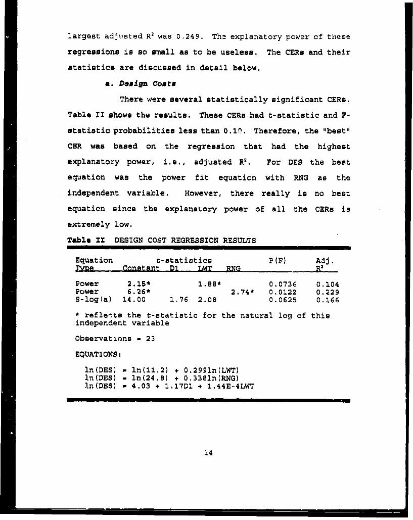
largest adjusted R2 was 0.249. The explanatory power of these
regressions is so small as to be useless. The CERs and their
statistics are discussed in detail below.
a. Design Costs
There were several statistically significant CERs.
Table II shows the results. These CERs had t-statistic and F-
statistic probabilities less than 0.1n. Therefore, the "best"
CER was based on the regression that had the highest
explanatory power, i.e., adjusted R2 . For DES the best
equation was the power fit equation with RNG as the
independent variable. However, there really is no best
equation since the explanatory power of all the CERs is
extremely low.
Table XX DESIGN COST REGRESSION RESULTS
Equation t-statistics P(F) Adj.Tyge Constant D1 LWT RNG R .
Power 2.15* 1.88* 0.0736 0.104Power 6.26* 2.74* 0.0122 0.229S-log(a) 14.00 1.76 2.08 0.0625 0.166
* reflects the t-statistic for the natural log of thisindependent variable
Observations - 23
EQUATIONS:
ln(DES) - ln(11.2) + 0.2991n(LWT)ln(DES) - ln(24.8) + 0.3381n(RNG)In(DES) - 4.03 + 1.17D1 * 1.44E-4LWT
14
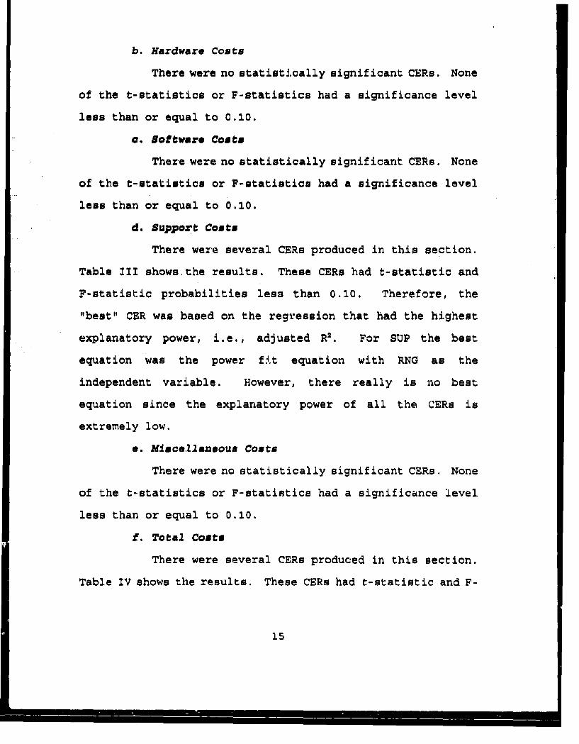
b. Hardware Costs
There were no statistically significant CERs. None
of the t-statistics or F-statistics had a significance level
less than or equal to 0.10.
a. Software Comst
There were no statistically significant CERs. None
of the t-statistics or F-statistics had a significance level
less than or equal to 0.10.
d. Support Costs
There were several CERs produced in this section.
Table III shows the results. These CERs had t-statistic and
F-statistic probabilities less than 0.10. Therefore, the
"best" CER was based on the regression that had the highest
explanatory power, i.e., adjusted R2. For SUP the best
equation was the power fV.t equation with RNG as the
independent variable. However, there really is no best
equation since the explanatory power of all the CERs is
extremely low.
e. Miscellaneous Costs
There were no statistically significant CERs. None
of the t-statistics or F-statistics had a significance level
less than or equal to 0.10.
f. Total Costs
There were several CERs produced in this section.
Table IV shows the results. These CERs had t-statistic and F-
15
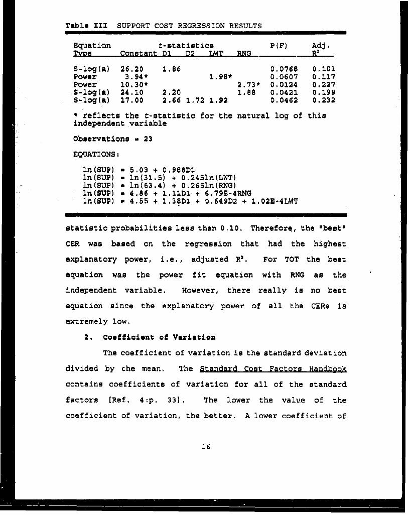
Table III SUPPORT COST REGRESSION RESULTS
Equation t-statistics P(F) Adj.Type Constant D1 D2 LWT RNG R2
S-log(a) 26.20 1.86 0.0768 0.101Power 3.94* 1.98* 0.0607 0.117Power 10.30* 2.73* 0.0124 0.227S-log(a) 24.10 2.20 1.88 0.0421 0.199S-log(a) 17.00 2.66 1.72 1.92 0.0462 0.232
* reflects the t-statistic for the natural log of thisindependent variable
Observations . 23
EQUATIONS:
ln(SUP) = 5.03 + 0.988D1ln(SUP) - ln(31.5) + 0.2451n(LWT)ln(SUP) a ln(63.4) + 0.2651n(RNG)ln(SUP) - 4.86 + 1.11D1 + 6.79E-4RNGln(SUP) - 4.55 + 1.38DI + 0.649D2 + 1.02E-4LWT
statistic probabilities less than 0.10. Therefore, the "best"
CER was based on the regression that had the highest
explanatory power, i.e., adjusted R1. For TOT the best
equation was the power fit equation with RNG as the
independent variable. However, there really is no best
equation since the explanatory power of all the CERs is
extremely low.
2. Coefficient of Variation
The coefficient of variation is the standard deviation
divided by che mean. The Standard Cost Factors Handbook
contains coefficients of variation for all of the standard
factors [Ref. 4:p. 33]. The lower the value of the
coefficient of variation, the better. A lower coefficient of
16
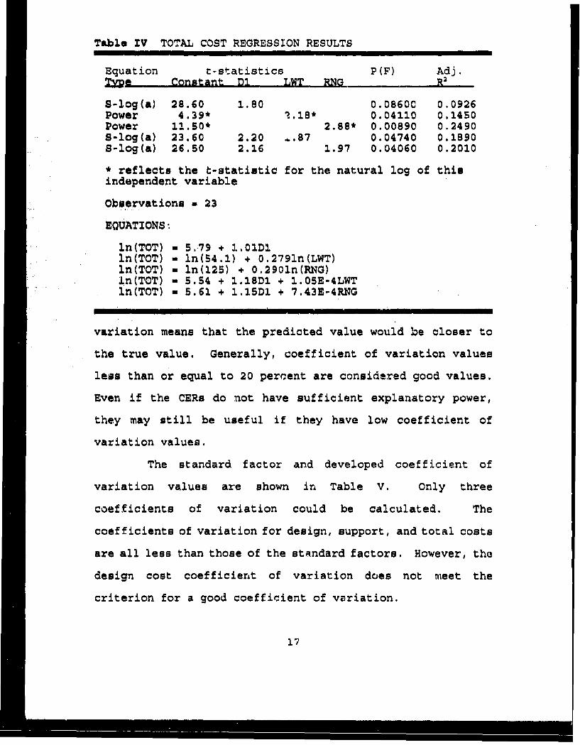
Table IV TOTAL COST REGRESSION RESULTS
Equation t-statistics P(F) Adj.. ~e Constant D1 LWT RNG R2
S-log(a) 28.60 1.80 0.08600 0,0926Power 4.39* 0.18* 0.04110 0.1450Power 11.50* 2.88* 0.00890 0.2490S-log(a) 23.60 2.20 ,.87 0.04740 0.1890S-log(a) 26.50 2.16 1.97 0.04060 0.2010
* reflects the t-statistic for the natural log of thisindependent variable
Observations - 23
EQUATIONS:
ln(TOT) - 5.79 + 1.01DIln(TOT) - ln(54.1) + 0.2791n(LWT)ln(TOT) - ln(125) + 0.2901n(RNG)ln(TOT) - 5.54 + 1.18DI + 1.05E-4LWTln(TOT) - 5.61 + 1.15DI + 7.43E-4RNG
variation means that the predicted value would be closer to
the true value. Generally, coefficient of variation values
less than or equal to 20 percent are considered good values.
Even if the CERs do not have sufficient explanatory power,
they may still be useful if they have low coefficient of
variation values.
The standard factor and developed coefficient of
variation values are shown in Table V. Only three
coefficients of variation could be calculated. The
coefficients of variation for design, support, and total costs
are all less than those of the standard factors. However, the
design cost coefficient of variation does not meet the
criterion for a good coefficient of variation.
17
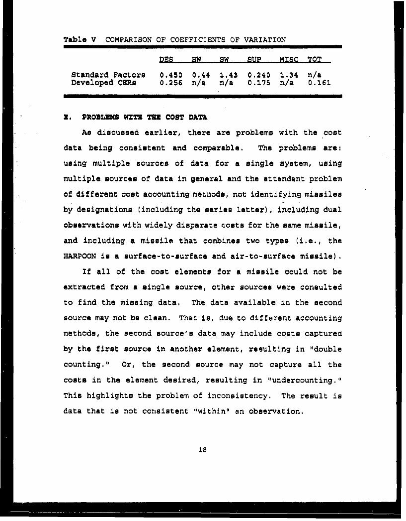
Table V COMPARISON OF COEFFICIENTS OF VARIATION
DES MW SW SUP MISC TOT
Standard Factors 0.450 0.44 1.43 0.240 1.34 n/aDeveloped CERs 0.256 n/a n/a 0.175 n/a 0.161
3. PROBL=X3 WITH THi COST DATA
As discussed earlier, there are problems with the cost
data being consistent and comparable. The problems are:
using multiple sources of data for a single system, using
multiple sources of data in general and the attendant problem
of different cost accounting methods, not identifying missiles
by designations (including the series letter), including dual
observations with widely disparate costs for the same missile,
and including a missile that combines two types (i.e., the
HARPOON is a surface-to-surface and air-to-surface missile).
If all of the cost elements for a missile could not be
extracted from a single source, other sources were consulted
to find the missing data. The data available in the second
source may not be clean. That is, due to different accounting
methods, the second source's data may include costs captured
by the first source in another element, resulting in "double
counting." Or, the second source may not capture all the
costs in the element desired, resulting in "undercounting."
This highlights the problem of inconsistency. The result is
data that is not consistent "within" an observation.
18
Multipl.e sources were consulted during the compilation of
the data, such as contractor's cost reports, cost estimates,
and budget data. Each source has its own methodology for
categorizing costs. This created the problem of nonstandard
data. The differences in categorization were relax.ed to the
purpose for which the reports were created. It is basically
impossible to break down these "wrapped up" categories into
the separate elements under study after the fact. The result
is data that cannot be compared by element. However, it is
possible that the total costs can be compared.
One of the most serious problems was that the missile for
which the cost data was collected was not identified by its
missile designator or series letter. This means that
technical and operational characteristics cannot be accurately
determined and matched to the cost data. In only one of the
23 observations was a missile designator and series letter
included. The rest just contained the missile name. There
was no way to tell for sure if the EMD cost data was for the
first missile in the series or for a later model. There were
also several missiles annotated with the acronym FSED (Pull
Scale Engineering Development). None of the resources
researched contained technical and operational characteristics
for missiles in this development stage. Therefore, the four
observations with this problem were either assigned the same
characteristics as the basic missile, or an assumption was
made to assign it the most recent model's characteristics. It
19
is evident that the validity of the data is in serious
question.
If two reliable sources were found for cost data for a
single missile, frequently both would be included as separate
observations. In all of the four pairs of missiles with dual
observations, the EMD costs for each element and the total
varied widely, seriously affecting the validity of the data.
For example, the PATRIOT missile had the following values for
the cost of design: $904M and $150M. There is a similar
discrepancy for the total costi $2,417M and $1,057M.
Obviously one observation is wrong. It is possible that both
are wrong. The question is, "Which one(s)?" The correction
to this problem is neither evident nor easy, since the data
are collected after the fact and require extraction from
reports and documents not created or maintained for this
purpose.
Finally, the last problem was whether an observation for
a missile that was composed of two types should be included.
The HARPOON missile is a surface-to-air and air-to-air
missile. The methodology used to track missile type used
dummy variables. However, there was no way to identify the
missile as having both type characteristics, so a separate
type was developed for it (D4 equal to one; DI, D2, D3 equal
to zero). This does not allow regression to consider the
effects of the HARPOON's surface-to-surface characteristics
with other surface-to-surface missiles or its air-to-surface
20
characteristics with other air-to-surface missiles. Instead,
it puts the HARPOON missile into a separate category, thereby
confounding the results, and not accomplishing the goal of
using missile type to predict EMD costs.
F. REGRESIzON WZTH "CLEAM)#R" DATA SST
As discussed in the above section, there are a lot of
problems inherent in the data. In this section, an attempt
will be made to make the data "cleaner" and then to analyze
the new data set to see if any usable results are present.
The "clean" terminology does not imply that the data set is
now valid. There are inherent problems with the data that
simple deletion of observations will not fix.
The original data set used was composed of 23
observations. The following nine observations were deleted to
create the cleaner data set: four FSED observations
(observations 10, 19, 20, 22), two dual observations
(observations 2, 13), and the HARPOON (observations 6, 7) and
PHOENIX AIM-56A (observation 15) missiles. The FSED and the
PHOENIX missile observations were deleted because no technical
data could be found. In the case of the dual observations,
the observations with the smaller costs were deleted from the
data base. It seems reasonable to assume that observations
with larger costs more accurately reflect true costs.
Finally, the HARPOON missile observations were deleted due to
21
the dual Missile type problem. This left 14 observations in
the data base, which are shown in Appendix B.
1. CER Development
Again, the initial evaluation criteria consisted of an
adjusted Ra greater than 0.90, absolute t-statistics greater
than two, and probability of the F-statistic (P(F)) lse. than
or equal to 0.05. Based on the low R2 values observed in the
results, the criteria were changed. The adjusted R2 criterion
was dropped. The t-statistic criterion was changed to the
probability of the t-statistic; both probabilities for the F-
statistic and t-statistic were changed to be less than or
equal to 0.10.
The results were still not encouraging. Only a few
cost estimating relationships were statistically significant.
The largest adjusted R2 was 0.342. The explanatory power of
these regressions is so small as to be useless. The CERs and
their statistics are listed below.
As discussed previously, use of IOC as an independent
variable may induce autocorrelation. This can be checked by
the Durbin-Watson statistic. Since IOC did not appear in any
of the final CERs, autocorrelation by definition is not a
problem.
a. Design Coste
There were several CERs produced in this section.
Table VI shows the results. These CERs had t-statistic and F-
22
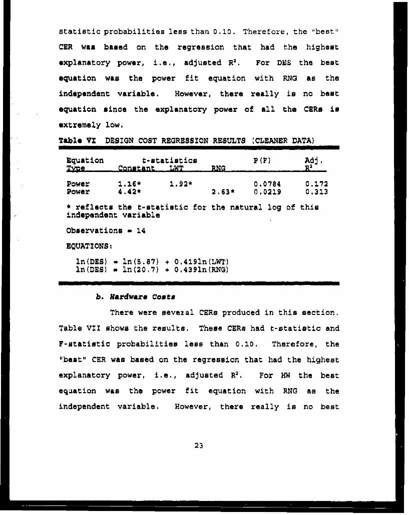
statistic probabilities less than 0.10. Therefore, the "best"
CER Was based on the regression that had the highest
explanatory power, i.e., adjusted R2 . For DES the best
equation was the power fit equation with RNG as the
independent variable. However, there really is no best
equation since the explanatory power of all the CERs is
extremely low.
Table V1 DESIGN COST REGRESSION RESULTS (CLEANER DATA)
Equation t-statistics P(F) Adj.Type Conastant LWT RNNG RPower 1.16* 1.92* 0.0784 0.172Power 4.42* 2.63* 0.0219 0.313
* reflects the t-statistic for the natural log of thisindependent variable
Observations = 14
EQUATIONS:
ln(DES) - ln(B.87) + 0.4191n(LWT)ln(DES) - ln(20,7) + 0.4391n(RNG)
b. Hardware Costs
There were several CERs produced in this section.
Table VII shows the results. These CERs had t-statistic and
F-statistic probabilities less than 0.10. Therefore, the
"best" CER was based on the regression that had the highest
explanatory power, i.e., adjusted R2. For HW the best
equation was the power fit equation with RNG as the
independent variable. However, there really is no best
23
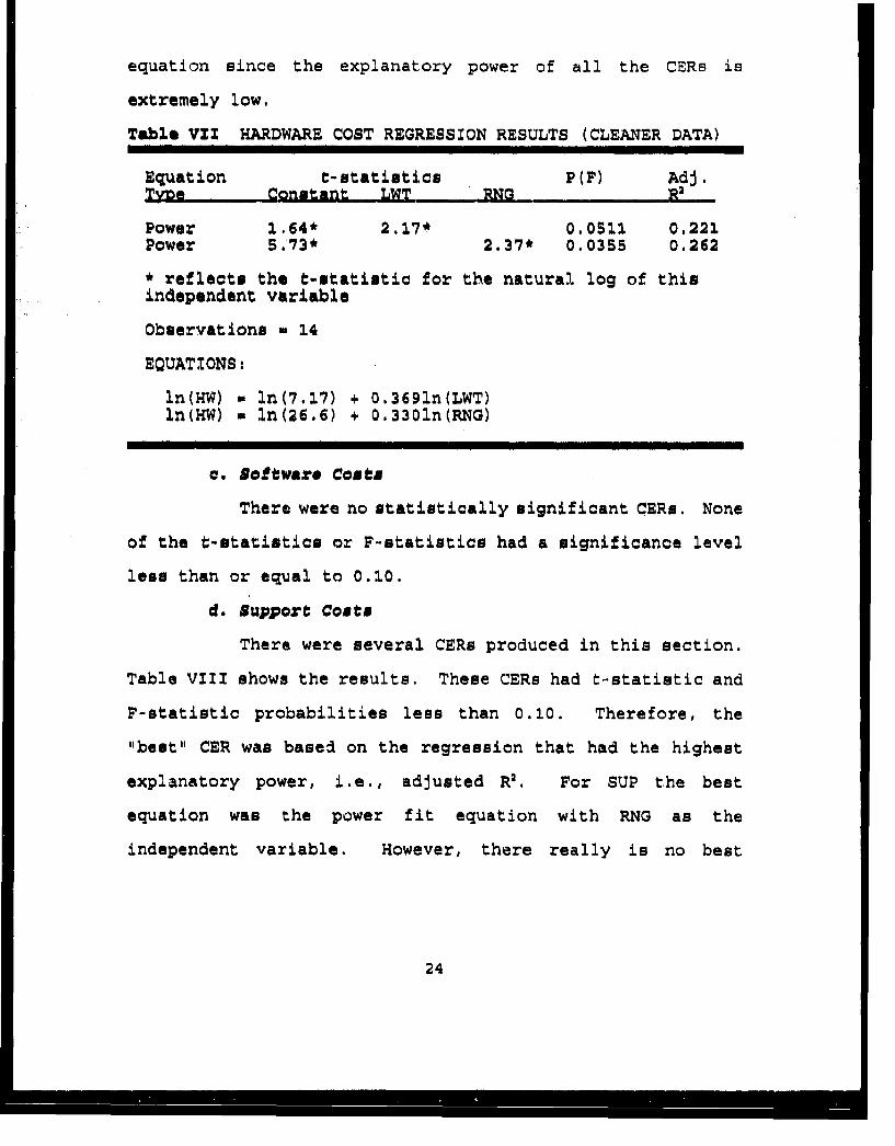
equation since the explanatory power of all the CERs is
extremely low,
Table VZ1 HARDWARE COST REGRESSION RESULTS (CLEANER DATA)
Equation t-statistics P(F) Adj.Type Constant LWT RNG R2
Power 1,64* 2.17* 0.0511 0.221Power 5.73* 2.37* 0.0355 0.262
* reflects the t-statistic for the natural log of thisindependent variable
Observations w 14
EQUATIONS:
ln(HW) - ln(7.17) + 0.3691n(LWT)ln(HW) w ln(26.6) + 0.3301n(RNG)
a. Software Costs
There were no statistically significant CERs. None
of the t-statistics or F-statistics had a significance level
less than or equal to 0.10.
d. Support Costs
There were several CERs produced in this section.
Table VIII shows the results. These CERs had t-statistic and
F-statistic probabilities less than 0.10. Therefore, the
"best" CER was based on the regression that had the highest
explanatory power, i.e., adjusted R1. For SUP the best
equation was the power fit equation with RNG as the
independent variable. However, there really is no best
24
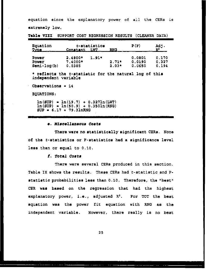
equation since the explanatory power of all the CERs is
extremely low.
Table VZZZ SUPPORT COST REGRESSION RESULTS (CLEANER DATA)
Equation t-statistics P(F) Adj.Tyoe Constant LWT RNaG R2
Power 2.4800* 1.91* 0.0801 0.170Power 7.4000* 2.71* 0.0190 0.327Semi-log(b) 0.0385 2.03* 0.0650 0.194
* reflects the t-statistic for the natural log of thisindependent variable
Observations - 14
EQUATIONS:
ln(SUP) - ln(19.7) + 0.3271n(LWT)ln(SUP) - ln(50.9) + 0.3501n(RNG)SUP I 6.17 + 79.31nRNG
e. Miscellaneous Costs
There were no statistically significant CERs. None
of the t-statistice or F-statistics had a significance level
less than or equal to 0.10.
f. Total Costs
There were several CERs produced in this section.
Table IX shows the results. These CERs had t-statistic and F-
statistic probabilities less than 0.10. Therefore, the "best"
CER was based on the regression that had the highest
explanatory power, i.e., adjusted R2 . For TOT the best
equation was the power fit equation with RNG as the
independent variable. However, there really is no best
25
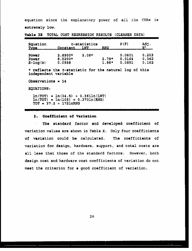
equation since the explanatory power of all the CERs is
extremely low.
Table XX TOTAL COST REGRESSION RESULTS (CLEANER DATA)
Equation t-statistics P(F) Adj.Constant LWT RNG R
Power 2.8900* 2.08* 0.0601 0.203Power 8.5200* 2.79* 0.0164 0.342S-log(b) 0.0988 1.88* 0.0851 0.162
* reflects the t-statistic for the natural log of thisindependent variable
Observations a 14
EQUATIONS:
ln(TOT) - ln(34.5) + 0.3611n(LWT)ln(TOT) - in(105) + 0.3701n(RNG)TOT - 37.2 + 1721nRNG
2. Coefficient of Variation
The standard factor and developed coefficient of
variation values are shown in Table X. Only four coefficients
of variation could be calculated. The coefficients of
variation for design, hardware, support, and total costs are
all less that those of the standard factors. However, both
design cost and hardware cost coefficients of variation do not
meet the criterion for a good coefficient of variation.
26
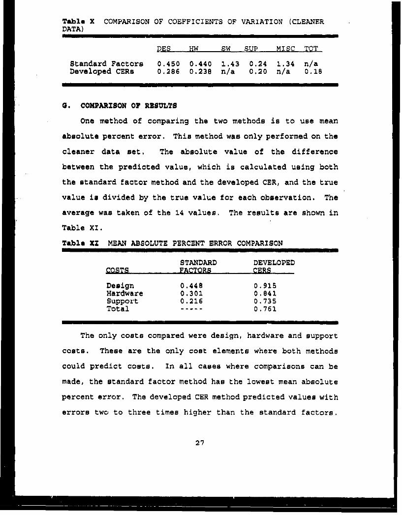
Table X COMPARISON OF COEFFICIENTS OF VARIATION (CLEANERDATA)
DES HW SW SUP MISC TOT
Standard Factors 0.450 0.440 1.43 0.24 1.34 n/aDeveloped CERs 0.286 0.238 n/a 0.20 n/a 0.18
0. COMPARISON OF RESULTS
One method of comparing the two methods is to use mean
absolute percent error. This method was only performed on the
cleaner data set. The absolute value of the difference
between the predicted value, which is calculated using both
the standard factor method and the developed CER, and the true
value is divided by the true value for each observation. The
average was taken of the 14 values. The results are shown in
Table XI.
Table XZ MEAN ABSOLUTE PERCENT ERROR COMPARISON
STANDARD DEVELOPEDCOSTS FACTORS CERS
Design 0.448 0.915Hardware 0.301 0.841Support 0.216 0.735Total ----- 0.761
The only costs compared were design, hardware and support
costs. These are the only cost elements where both methods
could predict costs. In all cases where comparisons can be
made, the standard factor method has the lowest mean absolute
percent error. The developed CER method predicted values with
errors two to three times higher than the standard factors.
27
For the total cost, the developed CERs predicted values with
a mean absolute percent error of 76.1%.
R. SUMMAaY
Based on the results of the analysis, it is clear that the
data collection process needs to be changed so that the data
is as consistent and comparable as possible. Missile
designations should clearly identify the missile for which
cost data is collected. Duplicate entries should be deleted.
Once this has been accomplished, a follow-on study should be
completed using the clean data. As it stands now, the data is
not suitable for regression analysis.
No significant physical or technical factors could be
determined due to the low explanatory power of the independent
variables. The highest adjusted R' was 24.9% for the initial
data set and 34.2% for the "cleaner" data set. Even though
the results are not statistically significant due to the low
adjusted R2s, the associated coefficients of variation are
lower than the standard factor coefficients of variation.
This means that these developed CERs may be better predictors
than the standard factors in use.
In the follow-on study, several factors can be added to
the model if the initial regressions are not statistically
significant. First, other independent variables, like length
of the missile or speed, could be added. If EMD costs do not
produce reasonable results, then perhaps percent of each cost
28
element might be studied. Finally, heteroscedasticity can be
a problem in cross-sectional data. One possibility to
consider is that the error variance may vary directly with an
independent variable, like launch weight. if this assumption
is true, the correction for heteroscedasticity would be
relatively easy and should be performed in the follow-on
study. It was not performed in this analysis, because of the
overwhelming question of data validity.
29
III. WARSHZP FUEL CONBSUPTION
A. PROBLEM DESCRIPTION
With the ending of the Cold War, the role of the U.S. Navy
has been under review to determine what is its mission. The
emphasis is changing from glo.bal conflicts to regional
conflicts. Attendant is the need to examine its force
structure. For example, should a new warship type or class be
created? Will it emulate existing ship types or be an
entirely new design? What is the operational cost of the new
warship? Since the 1970s no new warship types have been
introduced. The Navy has been satisfied with the current mix
and design of its seven warships, each type with the same
basic performance and physical characteristics. Estimates of
operational costs, such as fuel consumption, have been
relatively routine due to the availability of historical data.
Because of the aging of the fleet and the changing nature of
war, the current mix of ship types will become obsolete. Navy
planners are designing a new class of ship that is envisioned
as a replacement for either destroyers or cruisers for
deployment by 2008. Incorporating new technologies and having
the capability for combat in coastal waters will affect the
design of its physical and performance characteristics. [Ref.
9:p. 39] Currently, there are no CERs developed to predict
30
the fuel consumption of new warships based on performance and
physical characteristics.
The main reason for focusing on fuel consumption is that
it makes up a large part of the Operations and Support (O&S)
cost of a ship. In a new ship type, it may be one of the
hardest elements to predict, since the interaction of the
physical and performance characteristics may not be well known
with respect to fuel consumption. By examining historical
data on seven types of ships that make up the warship
category, this chapter will explore the relationship between
performance and physical characteristics and fuel consumption.
B. DESCRIPTION OP DATA
The regression model to be developed depends exclusively
on the data obtained. Two dependable sources of data were
identified: Navy Visibility And Management of Operating and
Support Costs (NAVY VAMOSC) and The Naval Institute Guide to
the Shins and Aircraft of the U.S. Fleet series. The VAMOSC
source contained OPTEMPO and fuel consumption data for the
fiscal years 1982 through 1)91 for all ships in the seven
warship types studied. The Naval Institute Guide series
contained physical and performance characteristics for the
ships contained in the VAMOSC database. The data from the two
sources were combined to provide input to the regression
model.
31
1. OPTEMPO And Fuel Consumption Data
NAVY VAMOSC collects O&S costs from all ships in the
active fleet. It does not include information on ships that
were inactive, commissioned, or deactivated during the fiscal
year. [Ref. 10:p. 1] The information is available in several
formats, such as the Individual Ships Report. The data used
was in the Individual Ships Report format for the following
warships: aircraft carriers (CV), battleships (BB), cruisers
(CO), destroyers (DD, DDG), and frigates (FF, FFG). Since the
focus was on fuel consumption, the following data fields were
"extracted for the fiscal years 1982 through 1991:
0 ship type
* class number
* hull number
* year
* steaming hours underway
* steaming hours not underway
* barrels of fuel consumed underway
* barrels of fuel consumed not underway
• total barrels of fuel consumed.
2. Physical and Performance Data
The following data was collected from T
Institute Guide to the Ships and Aircraft of the U.S. Fleet
for each ship in the VAMOSC data base:
32
• commissioning date (fiscal year)
* full load displacement
* overall length
* beam
* draft
* number of shafts
0 horsepower per shaft
• speed.
These independent variables will be discussed in greater
detail in a later section.
The independent variables listed above are considered
the more important ones. Obviously, others could have been
added. However, it was felt that they would not add
explanatory power to the model. Similarly, alternate
independent variables could have been used. For excample,
waterline length could have been substituted for overall
length. However, these alternate variables were missing some
observations. Since incomplete data would adversely affect
the analysis and other similar variables with a complete set
of observations were available, the alternate variables were
not used.
A new independent variable, total shaft horsepower
(TSHP), was calculated from this data. Total shaft horsepower
was the number of shafts multiplied by the horsepower per
shaft. Knowing how much total horbepower the propulsion
33
system provided provides a means for comparing ships that had
different numbers of shafts and/or shaft horsepower with a
single variable.
The commissioning date was included so that another
new variable, age (AGE), could be calculated. AGE represents
the level of technology and required maintenance. It was
calculated by subtracting the ship's commissioning date from
each fiscal year that it operated as provided by the VAMOSC
data. Therefore, the ship's age would be a proxy for the
level of technology and required maintenance.
3. ConstzuctLng the Znitial Data Same
The first step in the analysis process was to explore
the properties of the data obtained from Navy VAMOSC before
performing regression on the combined data base. Each ship
type consisted of several classes, which in turn contained
many individual ships, resulting in hundreds of observations.
A major problem was how to structure the data so that it could
be easily analyzed. The simplest method was to construct a
separate data base for each ship type. Seven separate data
bases, each consisting of one type of ship, were created.
Each data base contained the following five OPTEMPO and fuel
consumption variables, steaming hours underway, steaming hours
not underway, barrels of fuel consumed underway, barrels of
fuel consumed not underway, and total barrels of fuel
consumed; plus the year for which the observation was
34
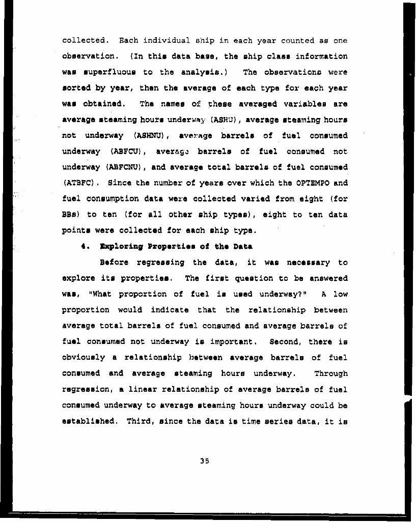
collected. Each individual ship in each year counted as one
observation. (In this data base, the ship class information
was superfluous to the analysis.) The observations were
sorted by year, then the average of each type for each year
was obtained. The names of these averaged variables are
average steaming hours underway (ASHU), average steaming hours
not underway (ASHNU), average barrels of fuel consumed
underway (ABFCU), aver&a barrels of fuel consumed not
underway (ABFCNU), and average total barrels of fuel consumed
(ATBFC). Since the number of years over which the OPTEMPO and
fuel consumption data were collected varied from eight (for
BBs) to ten (for all other ship types), eight to ten data
points were collected for each ship type.
4. Exploring Properties of the Data
Before regressing the data, it was necessary to
explore its properties. The first question to be answered
was, "What proportion of fuel is used underway?" A low
proportion would indicate that the relationship between
average total barrels of fuel consumed and average barrels of
fuel consumed not underway is important. Second, there is
obviously a relationship between average barrels of fuel
consumed and average steaming hours underway. Through
regression, a linear relationship of average barrels of fuel
consumed underway to average steaming hours underway could be
established. Third, since the data is time series data, it is
35
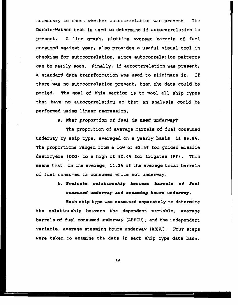
necessary to check whether autocorrelation was present. The
Durbin-Watson test is used to determine if autocorrelation is
present. A line graph, plotting average barrels of fuel
consumed against year, also provides a useful visual tool in
checking for autocorrelation, since autocorrelation patterns
can be easily seen. Finally, if autocorrelation was present,
a standard data transformation was used to eliminate it. If
there was no autocorrelation present, then the data could be
pooled. The goal of this section is to pool all ship types
that have no autocorrelation so that an analysis could be
performed using linear regression.
a. Whae proportion of fuel Is used underway?
The proportion of average barrels of fuel consumed
underway by ship type, averaged on a yearly basis, is 85.8%.
The proportions ranged from a low of 82.3% for guided missile
destroyers (DDG) to a high of 90.4% for frigates (FF). This
means that, on the average, 14.2% of the average total barrels
of fuel consumed is consumed while not underway.
b. Evaluate relationship between barrels of fuel
consumed underway and steamilng hours underway.
Each ship type was examined separately to determine
the relationship between the dependent variable, average
barrels of fuel consumed underway (ABFCU), and the independent
variable, average steaming hours underway (ASHU). Four steps
were taken to examine the data in each ship type data base.
36
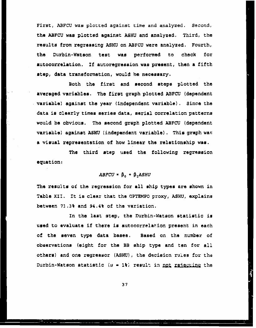
First, ABFCU was plotted against time and analyzed. Second,
the ABFCU was plotted against ASHU and analyzed. Third, the
results from regressing ASHU on ABFCU were analyzed. Fourth,
the Durbin-Watson test was performed to check for
autocorrelation. If autoregression was present, then a fifth
step, data transformation, would be necessary.
Both the first and second steps plotted the
averaged variables. The first graph plotted ABFCU (dependent
variable) against the year (independent variable). Since the
data is clearly times series data, serial correlation patterns
would be obvious. Tho second graph plotted ABFCU (dependent
variable) against ASHU (independent variable). This graph war
a visual representation of how linear the relationship was.
The third step used the following regression
equation:
ABFCU o ÷+ 1ASHU
The results of the regression for all ship types are shown in
Table XII. It is clear that the OPTEMPO proxy, ASHU, explains
between 72.3% and 94.4% of the variation.
In the last step, the Durbin-Watson statistic is
used to evaluate if there is autocorrelation present in each
of the seven type data bases. Based on the number of
observations (eight for the BB ship type and ten for all
others) and one regressor (ASHU), the decision rules for the
Durbin-Watson statistic (u - lV result in = Ir-.Zjeuin the
3?
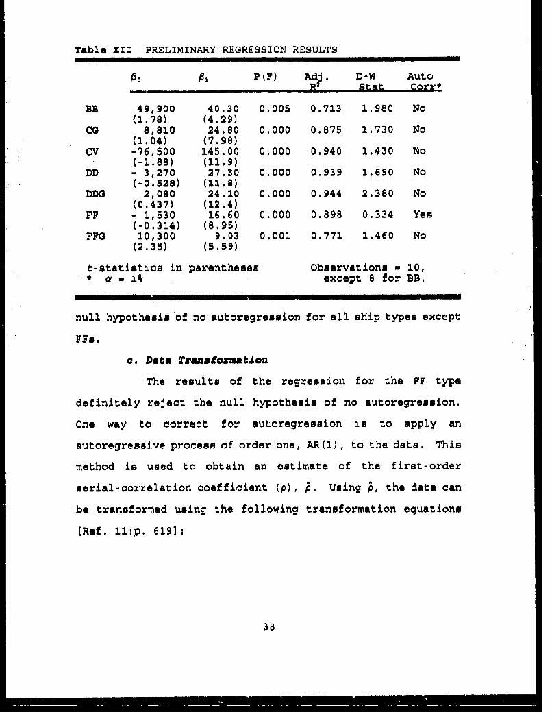
Table XII PRELIMINARY REGRESSION RESULTS
00 9 P(F) Adj. D-W Auto.. R2 Stat Corr*
BB 49,900 40.30 0.005 0.713 1.980 No(1.78) (4.29)
CG 8,810 24.80 0.000 0.875 1.730 No(1.04) (7.98)
CV -76,500 145.00 0.000 0.940 1.430 No(-1.88) (11.9)
DD - 3,270 27.30 0.000 0.939 1.690 No(-0.528) (11.8)
DDG 2,080 24.10 0.000 0.944 2.380 No(0.437) (12.4)
PF - 1,530 16.60 0,000 0.898 0.334 Yes(-0.314) (8.95)
FFG 10,300 9.03 0.001 0.771 1.460 No(2.35) (5.59)
t-statistics in parentheses Observations m 10,* •- 1% except 8 for BB,
null hypothesis of no autoregression for all ship types except
a. Data Transformation
The results of the regression for the FF type
definitely reject the null hypothesis of no autoregression.
One way to correct for autoregression is to apply an
autoregressive process of order one, AR(1), to the data. This
method is used to obtain an estimate of the first-order
serial-correlation coefficient (p), b. Using b, the data can
be transformed using the following transformation equations
[Ref. llhp. 619)
38
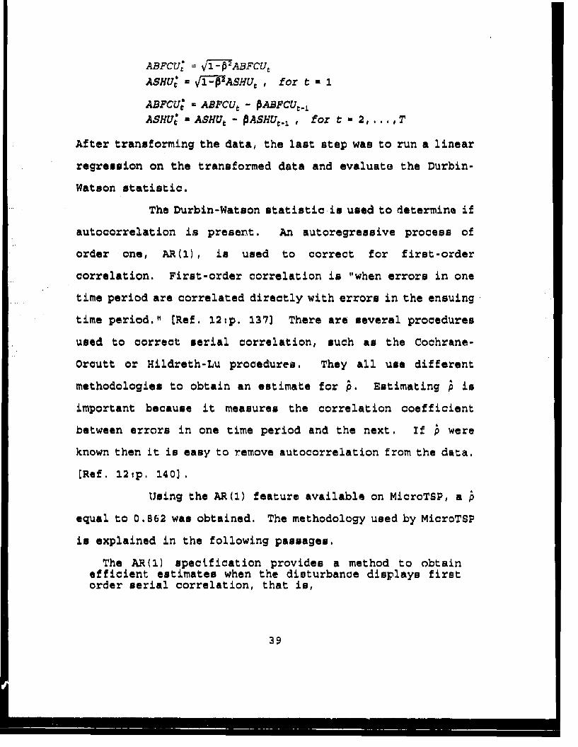
ABFCU; = VT0ABFCU
ASHUt = V1FPASHUt , for t - 1
ABFCUt = ABFCUt - PABFCUt.IASHUt - ASHU A - PASHU.i , for t -2,,2 ,T
After transforming the data, the last step was to run a linear
regression on the transformed data and evaluate the Durbin-
Watson statistic.
The Durbin-Watson statistic is used to determine if
autocorrelation is present. An autoregressive process of
order one, AR(1), is used to correct for first-order
correlation. First-order correlation is "when errors in one
time period are correlated directly with errors in the ensuing
time period." [Ref. 12:p. 137) There are several procedures
used to correct serial correlation, such as the Cochrane-
Orcutt or Hildreth-Lu procedures. They all use different
methodologies to obtain an estimate for b. Estimating ý is
important because it measures the correlation coefficient
between errors in one time period and the next. If b were
known then it is easy to remove autocorrelation from the data.
(Ref. 121p. 140).
Using the AR(1) feature available on MicroTSP, a
equal to 0.862 was obtained. The methodology used by MicroTSP
is explained in the following passages.
The AR(1) specification provides a method to obtainefficient estimates when the disturbance displays firstorder serial correlation, that is,
39
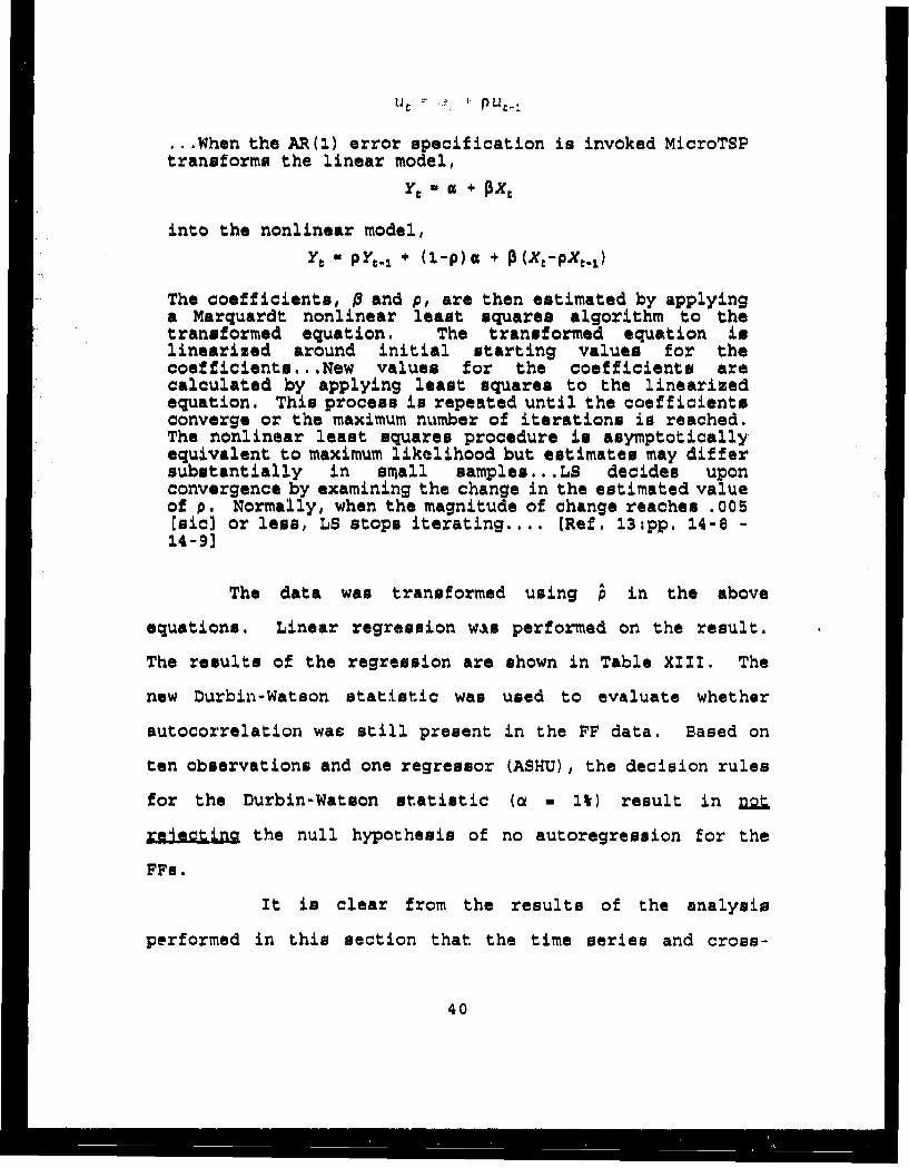
U t pUt.
... When the AR(1) error specification is invoked MicroTSPtransforms the linear model,
Ye a +
into the nonlinear model,
*t+ pre. + (l-P) a + P(XC-PXt.1)
The coefficients, 0 and p, are then estimated by applyinga Marquardt nonlinear least squares algorithm to thetransformed equation. The transformed equation islinearized around initial starting values for thecoefficients...New values for the coefficients arecalculated by applying least squares to the linearizedequation. This process is repeated until the coefficientsconverge or the maximum number of iterations is reached.The nonlinear least squares procedure is asymptoticallyequivalent to maximum likelihood but estimates may differsubstantially in siall samples...LS decides uponconvergence by examining the change in the estimated valueof p. Normally, when the magnitude of change reaches .005[sic] or less, LS stops iterating.... (Ref. 13:pp. 14-8 -14-91
The data was transformed using P in the above
equations. Linear regression was performed on the result.
The results of the regression are shown in Table XIII. The
new Durbin-Watson statistic was used to evaluate whether
autocorrelation was still present in the FF data. Based on
ten observations and one regressor (ASHU), the decision rules
for the Durbin-Watson statistic (i - I%) result in not
g the null hypothesis of no autoregression for the
FFs.
It is clear from the results of the analysis
performed in this section that the time series and cross-
40
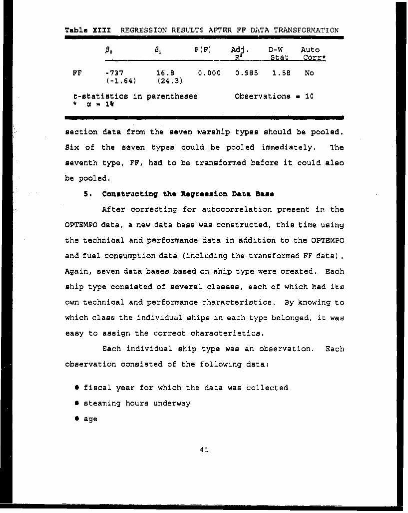
Table XIII REGRESSION RESULTS AFTER FF DATA TRANSFORMATION
go 0 P(F) Adj. D-W Auto- P. Stat Corr*
FF -737 16.8 0.000 0.985 1.58 No(-1.64) (24.3)
t-statistics in parentheses Observations - 10* •- U
section data from the seven warship types should be pooled.
Six of the seven types could be pooled immediately. The
seventh type, FF, had to be transformed before it could also
be pooled.
5. Constructing the Regression Data Base
After correcting for autocorrelation present in the
OPTEMPO data, a new data base was constructed, this time using
the technical and performance data in addition to the OPTEMPO
and fuel consumption data (including the transformed FF data).
Again, seven data bases based on ship type were created. Each
ship type consisted of several classes, each of which had its
own technical and performance characteristics. By knowing to
which class the individual ships in each type belonged, it was
easy to assign the correct characteristics.
Each individual ship type was an observation. Each
observation consisted of the following data:
0 fiscal year for which the data was collected
* steaming hours underway
* age
41
9 full load displacement
* overall length
* beam
* draft
* total shaft horsepower
* speed.
The observations in each ship type data base were
sorted by year and averages were taken of the yearly data.
The result was eight (for BBs) or ten (for all other ship
types) yearly: averaged observations per ship type. These
sixty-eight averaged observations comprised the regression
data base. This data is contained in Appendix C.
C. DEVELOPMENT OF THE MODEL
In developing a basic model for fuel consumption, certain
a priori expectations are held about the independent variables
included in the estimation equation:
ABFCU = f (ASHU, AGE, DISPFL, LENOA. BEAM, DRAFT, TSHP, SPEED)
Although there are several other independent variables
representing the physical and performance factors, these seven
variables were the most likely to be available for new ships
and were directly related to fuel consumption.
1. Average Steaming flours Underway (ASHU)
Average steaming nour- underway is a measure of the
OPTEMPO of Uhe ship. Tt- 1 the average number of hours
--teamed underway for each year a ship of a particular ship
type wz.,' operated. It is reasonable to expect that the
OPTEMPO of the ship would affect the fuel consumption. For
instance, the higher the average number of hours steamed
underway, the higher the average number of barrels of fuel
consumed. The variable is measureu in hours.
"~. Age.
Age is a proxy for the level of technology and
mainte'nance level of the ship. It ii reasonable to expect
that '-ie newer the ship, the more r.•, technology in ship
propulsion and naval engineering could be incorporated into
the design. it is also the case that the newer the ship the,
more likely it has not gone through its maintenance cycle.
Both of the reasons would be expected to affect the fuel
consumption. For example, the older the ship, the less fuel
efficient it would be. The variable is measured in years.
3. Full Load Displaaoment (DISPFL)
Full load displacement in the displacement of a fully
loaded ship ready to steam into service and perform its
missio-n. [Ref. 14:p. 13) It is expected that the displacement
of the ship would affect the fuel consumption. For example,
the heavier the ship, the more fuel would be needed to sail
the ship. The variable ic measured in tons.
43
4. Overall Length (LENOA)
The overall length of a ship is measured at the
longest part of the ship. [Ref. 14:p. 13) It is expected that
the length of the ship would affect the fuel consumption. For
example, the longer the ship, the larger the ship. It is
expected that larger ships would consume more fuel since they
have larger masses to push forward in the water. The variableis measured in meters.
5. beam
The beam is measured at the most extreme width of the
ship's hull. [Ref. 14:p. 13) It is expected that the wider
the beam, the more fuel would be consumed. The width of the
ship would act as a braking force in the water, requiring more
power (which requires more fuel) to push it forward, The
variable is measured in meters.
6. Draft
The draft of the ship is the maximum draft of the ship
at full load and includes fixed projections under the keel.
[Ref. 14:p. 13) Tt is expected that the depth of the ship's
draft would affect the fuel1 consumption, For example, the
deeper the draft, the more mass under the waterline. The
draft. would a&t as a braking force in the water, requiring
more power (which requires more fuel) to push it forward. The
variable is measured in meteis.
44.
7. Total Shaft Horsepower (TSHP)
Total shaft horsepower is a deri.ved variable obtained
by multiplying the number of shafts for a ship by its shaft
horsepower. This value is the total horsepower supplied by
the propulsion plant. It is expected that the size of the
power plant would affect the fuel consumption. For example,
a larger power plant would be expected to consume more fuel.
The variable is measured in horsepower.
S. Speed
The speed is the maximum speed that a ship class is
capable of operating at. [Ref. 15:p. 142 It is expected that
the ship's speed would affect the fuel consumption. For
example, the faster the speed, the less fuel efficient the
ship. The variable is measured in knots.
The specified form of the basic model follows;
ABFCU - PO + PIASHU + NAGE + P3DISPFL + P4LENOA + PsBEAM+ PDRAFT + P7 TSHP + PaSPEED
The criteria for identifying the best model is the one with
high t.statistics, adjusted R2, and F-statistics,
respectively, with as few independent variables as possible.
For the purposes of this chapter, the benchmarks for the
criteria are absolute t-statistics greater than or equal to
two, adjusted R2 values greater than or equal to 0.90 and the
probability of the F-statistic less than 0.000.
45
Three independent variables are considered to be crucial
to the model: ASHU, AGE, and DISPFL. The basic model
includes eight independent variables. However, four (DISPFL,
LENOA, BEAM, DRAFT) may be correlated and create potential
multicollinearity in the model. The presence of
multicollinearity-will make it difficult (if not impossible)
to interpret the regression coefficients. The presence of
.multicollinearity may be reduced and, perhaps, eliminated by
deleting one or more of the fout independent variables. This
will be discussed in the alternative specifications section.
Whenever time-series data is used, autocorrelation may be
a problem, The data set used in this analysis was constructed
to eliminatethe presence of autocorrelation, as discussed in
a prior section. In interpreting the results of the following
regressions, the methodology uA. data c',,nstruction must be kept
in mind.. For this data set, the Durbin-Watson statistic will
be meaningless, since this final data set consists of pooled
time-series and cross-section observations. The Durbin-Watson
statistic is useful only on true first order autocorrelated
data. Because of this deliberate construction and because the
time series are short (at most ten observations) and there
were only seven ship types, autocorrelation is ignored.
Typically, a priori expectations about the sign of the
coefficients are held. These were discussed in the above
section. The expected sign hypotheses are listed in Table
XIV.
46
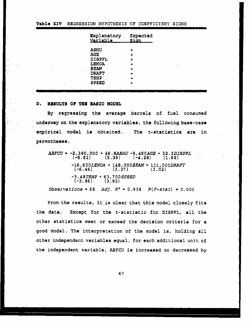
Table XIV REGRESSION HYPOTHESIS OF COEFFICIENT SIGNS
Explanatory ExpectedVariable Sian,
ASHU +AGE +DISPFL +LENOA +BEAM +DRAFT +TSHP +SPEED +
D. RESULTS OF THE BASIC MODEL
By regressing the average barrels of fuel consumed
underway on the explanatory variables, the following base-case
empirical model is obtained. The t-statistics are in
parentheses.
ABFCU a -2,380,000 4 6,. SASHU -549OAGE + 3 2S3 DISFL(-5.61) (5,39) (-4.28) (1.68)
-16,60OLENOA + 148, OOOBEAM + 111i, OOODRAFT(-6,46) (3.37) (3.02)
"-3.48TSHP + 63,700SPEED(-3,86) (3,92)
Observations - 68 Adj. R2 - 0.938 P(F-stat) w 0.000
From the results, it is clear that this model closely fits
the data. Except for the t-statistic for DISPFL, all the
other statistics meet or exceed the decision criteria for a
good model. The interpretation of the model is, holding all
other independent variables equal, for each additional unit of
the independent variable, ABFCU is increased or decreased by
47
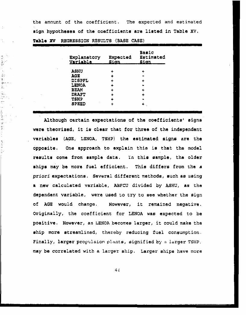
the amount of the coefficient. The expected and estimated
sign hypotheses of the coefficients are listed in Table XV.
Table XV REGRESSION RESULTS (BASE CASE)
BasicExplanatory Expected EstimatedVariable Sign Sign
ASHU + +AGE + -DSPFL + +LENOA + -
BEAM + +DRAFT + +TSHP + -
SPEED + +
Although certain expectations of the coefficients' signs
were theorized, it is clear that for three of the independent
variables (AGE, LENOA, TSHP) the estimated signs are the
opposite. One approach to explain this is that the model
results come from sample data. in this sample, the older
ships may be more fuel efficient. This differs from the a
priori expectations. Several different methods, such as using
a new calculated variable, ABFCU divided by ASHU, as the
dependent variable, were used to try to see whether the sign
of AGE would change. However, it remained negative.
originally, the coefficient for LENOA was expected to be
positive. However, an LENOA becomes larger, it could make the
ship more streamlined, thereby reducing fuel consumption,
Finally, larger propulsion plants, signified by a larger TSHP,
may be correlated with a larger ship. Larger ships have more
46
mass to push through the water and therefore may consume more
fuel. With this explanation a negative coefficient for TSHP
would be expected.
E. ALTERNATZVE SPECIFICATZONS
Although the results of the basic model are very good,
there is some question about whether all eight independent
variables are necessary, specifically TSHP and SPEED.
Accordingly, three alternative cases will be examined. The
first alternative model deletes SPEED as an independent
variable. The second alternative model deletes TSHP. The
third alternative model deletes both TSHP and SPEED. The
results are shown in Appendices D through G.
Within the base case and the three alternative models, it
is important to check whether multicollinearity exists between
DISPFL, LENOA, BEAM, and DRAFT. In each of these four models
the following combinations of the independent variables were
deleted from the model:
0 LENOA
* BEAM
* DRAFT
• BEAM, DRAFT
* LENOA, DRAFT
* LENOA, BEAM
* LENOA, BEAM, DRAFT,
49
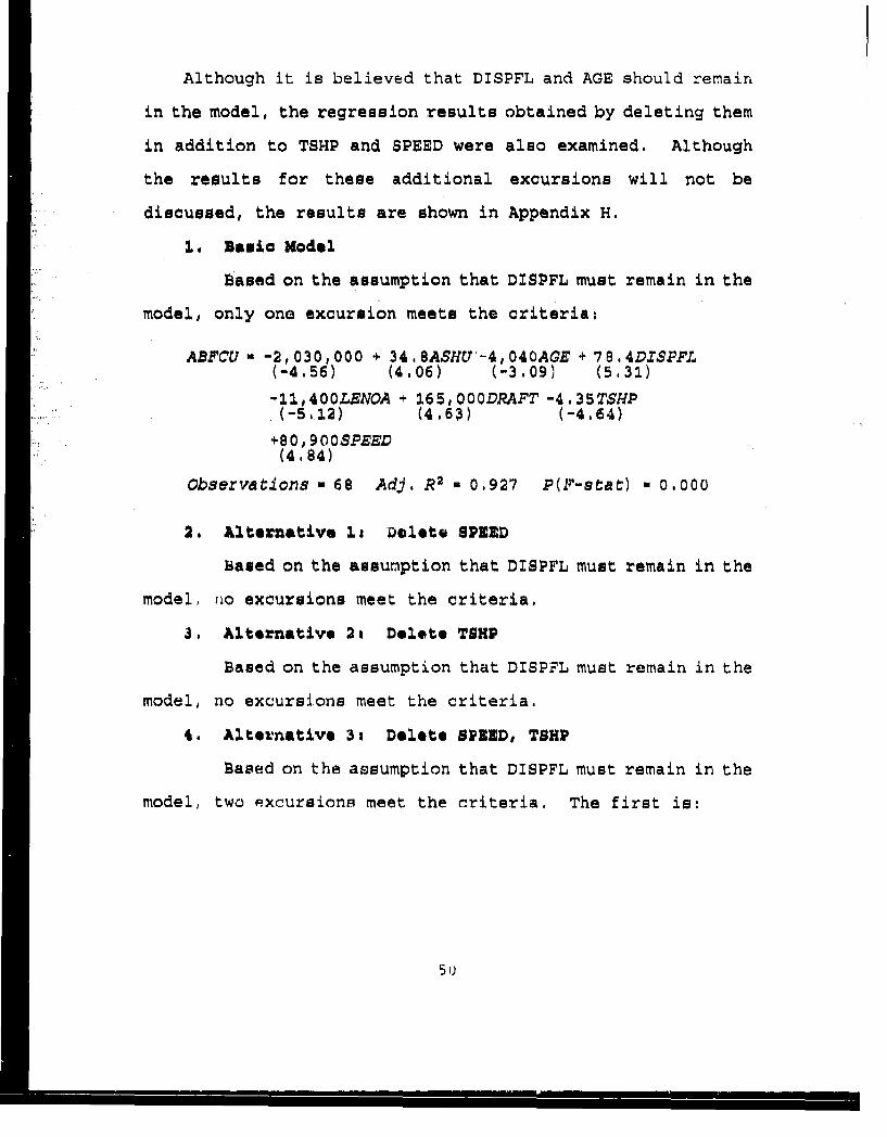
Although it is believed that DISPFL and AGE should remain
in the model, the regression results obtained by deleting them
in addition to TSHP and SPEED were also examined. Although
the results for these additional excursions will not be
discussed, the results are shown in Appendix H.
1. Basic Model
Based on the assumption that DISPFL must remain in the
model, only one excursion meets the criteria:
ABFCU( -2#•30,000 + 34.8ASHU-4,04OAGE + 78.4DIS.PFL(-4,56) (4.06) (-3.09) (5.31)
-ll,40OLEAOA + l65,OOODRAFT -4.3STSH.P
+80, 900SPEED(4.84)
Observations - 68 Adj. R2 - 0.927 P(F-stat) . 0.000
2. Altezrative 1i Delete SPEED
Based on the assumption that DISPFL must remain in the
model, ro excursions meet the criteria.
3. Alternative 2t Delete TSHP
Based on the assumption that DISPFL must remain in the
model, no excursions meet the criteria.
4. Alternative 31 Delete SPEND, TSHP
Based on the assumption that DISPFL must remain in the
model, two excursions meet the criteria. The first is:
5 u
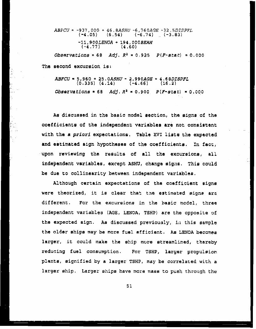
ABFCU = -937,000 + 46.8ASHU -6,760AGE -32.5DISPFL(-4.05) (6,54) (-6,74) (-3.83)
-11,900LENOA + 194,OOOBEAM(-4.77) (4,60)
Observations = 68 Adj. R 2 = 0.925 P(F-stat) = 0.000
The second excursion is:
ABFCU 5,960 + 25.0ASHU - 2,990AGE + 4.6 8DISPFL(0.335) (4.14) (-4.66) (16.2)
Observations * 68 Adj, R2 - 0.900 P(F-stat) * 0.000
As discussed in the basic model section, the signs of the
coefficients of the independent variables are not. consistent
with the apriori expectations. Table XVI lists the expected
and estimated sign hypotheses of the coefficients. in fact,
upon reviewing the results of all the excursions, all
independent variables, except ASHU, change signs. This could
be due to collinearity between independent variables.
Although certain expectations of the coefficient signs
were theorized, it is clear that thie estimated signs are
different. For the excursions in the basic model, three
independent variables (AGE, LENOA, TSHP) are the opposite of
the expected sign. As discussed previously, in this sample
the older ships may be more fuel efficient. As LENOA becomes
larger, it could make the ship more streamlined, thereby
reducing fuel consumption. For TSHP, larger propulsior
plants, signified by a larger TSHP, may be correlated with a
larger ship. Larger ships have more mass to push through the
51
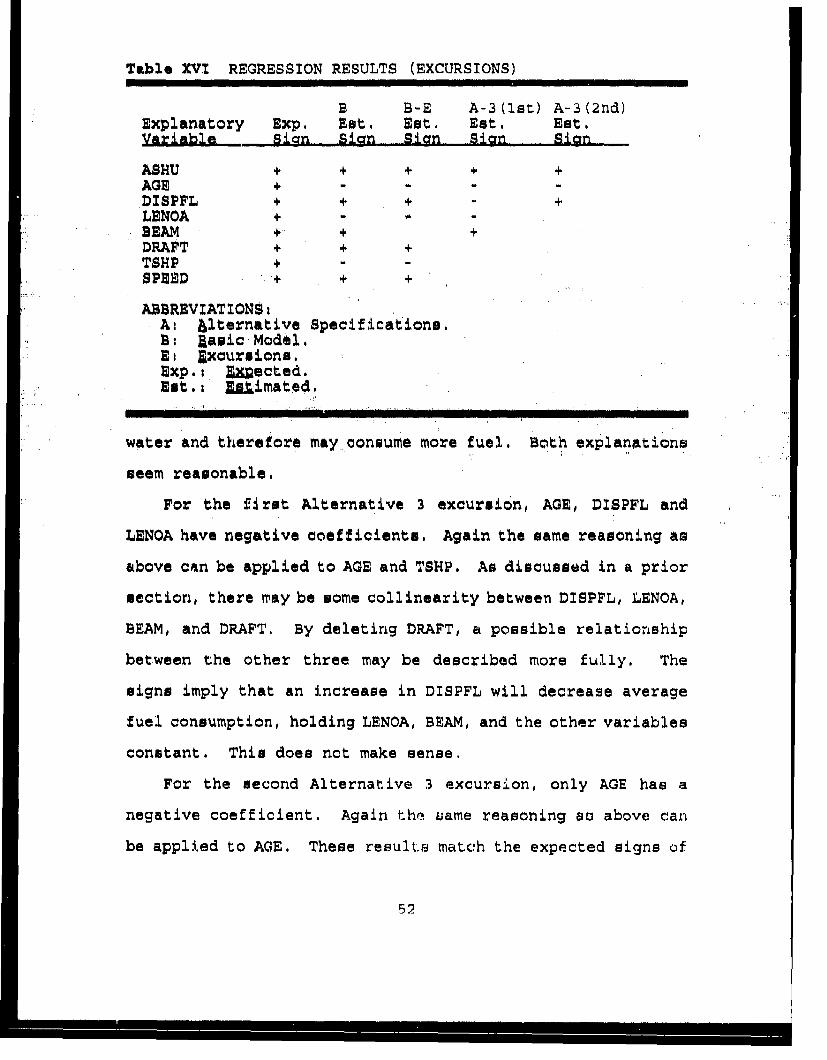
Table XVI REGRESSION RESULTS (EXCURSIONS)
B B-E A-3(1st) A-3(2nd)Explanatory Exp. Eat. Est. Est. Est.Variable, Sign Sian Sian Sign Sign
ASHU + + + + +AGE + ....DISPFL + + - +LENOA + - -
BEAM + +DRAFT + + +TSHP + - -
SPEED 4 + +
ABBREVIATIONS:At <ernative Specifications.B: lasic Model.Ei &xcursions.Exp.i Saected.Est.: Ej.=imateO.
water and therefore may consuMe more fuel, Both explanations
seem reasonable.
For the first Alternative 3 excursion, AGE, DISPFL and
LENOA have negative coefficients, Again the same reasoning as
above can be applied to AGE and TSHP. As discussed in a prior
section, there may be some collinearity between DISPFL, LENOA,
BEAM, and DRAFT. By deleting DRAFT, a possible relationship
between the other three may be described more fully. The
signs imply that an increase in DISPFL will decrease average
fuel consumption, holding LENOA, BEAM, and the other variables
constant. This does not make sense.
For the second Alternative 3 excursion, only AGE has a
negative coefficient. Again the uame reasoning au above can
be applied to AGE. These result.s match the expected signs of
52
the variables much better than the previous excursions. The
estimated equation also contains the fewest independent
variables. Based on these two results, this equation is
chosen as the best model.
P6* HRTZROSCEDASTICITYi•1 . Definition
Heteroscedasticity violates one of the assumptions for
a normal linear regression model, resulting in the model being
incorrectly specified. The parameter estimates will be
unbiased and consistent, but not efficient.
Heteroscedasticity is non-constant variance of the error term.
"[Ref. 12:pp. 127-128) For example, the variance of the error
terms associated with larger ships may be larger than the
variance of the error terms associated with smaller ,ships.
Since the data are pooled time-series, cross-section
observations, we expect that pure heteroscedasticity may be
difficult to remove, There are several tests to check for
heteroscedasticity. One is the Goldfeld-Quandt test.
The Goldfeld-Quandt test procedure estimates two
regression lines, one using data thought to come from the data
with low variance errors and the other from data with high
variance errors. The residual sum of squares is calculated
for each regression, i.e., ESSH± and ESSLo. The new test
statistic, ESSHi/ESSL,C, is distributed an an F-statistic, The
number of degrees of freedom in the general linear case is:
53
N-d-2k
where N is the number of observations, d is the number cf
middle observations deleted, and k is the number of
independent variables (including the constant term). The null
hypothesis is that there is homoscedasticity. The alternative
hypothesis is that the variance (a,) varies by some function
of an independent variable (X) for each observation (0):
0.2 f t( 1
The null, hypothesis can not be rejected if the residual
variances of the two lines are approximately equal. it. is
rejected when the calculated statistic is greater than the
critical value of the P distribution. [Ref. 12tp. 133)
2. Cro•ecton
Using the GoldfLLe Qm:~'~i' tst, the best model from
the previous section was tested for heteroscedasticity. The
initial assumption was that the independent variable DISPFL
was associated with the error variance. Two regressions were
performed, one on the 27 largest observations and one on the
smallest 27 observations. The result is an F-statistic of
173, clearly rejecting the null hypothesis of homoscedasticity
at any level of significance. This result makes intuitive
sense. The next step tried to correct the heteroscedasticity.
As previously dificussed, there may be some
relationship between the error variances and one of the
54
independent variables. It is reasonable to conclude that
DISPFL could be that variable. If this is true, then there is
an easy transformation to correct the heteroscedasticity
present in the data. (Ref. 12:p. 130) One way to determine
the form of the function is to create a scatter plot, plotting
the residuals of the best equation versus DISPFL. Depending
on the shape of the scatter plot, it may be possible to
recognize the function that describes it.
No pattern was recognizable in the scatter plot of the
residuals and DISPFL, so an assumption was made to use the
following transformation:
Var(ed)w C*DISPFL2, where C = a nonzero constant
The process is straightforward. Once the independent variable
is identified, in this case DISPFL, all the terms in the
original regression equation are divided by it. The Goldfeld-
Quandt test is used again to test whether the transformation
corrected the heteroscedasticity. The same test statistic
described previously is used to decide whether or not to
reject the null hypothesis. If the assumption of the
transformation form is correct, the null hypotheses will not
be rejected. Since the homoscedasticity assumption would no
longer be violated, the resulting parameter estimates will be
efficient. [Ref. 12:pp. 130-1311
The results of this transformation showed that the
null hypothesis was rejected. Heteroscedasticity could not be
55
corrected by the square of DISPFL. This same methodology was
performed on the other two independent variables in the
equation, AS14UJ and AGE. The results were the same:
heteroscedasticity in the original equation,
heteroscedabticity after the transformation.
Aflothe.," way to deal with heteroscedastiuLty is to use
a heteroscedasticity consistent covariance matrix with the
least squares regression instead of the one normally used to
calculate stardard errors and t-statistics. The ore used by
MicroTSP is the White covariance matrix [Ref. 13:p. 14-6):
nnk ) (X'X) "•(ex ' (X'X) "
where n number of observationsk number of..regressorsi least squares residual
This method corrects the heteroscedasticity problem 6o that
the results may be interpreted correctly. The White test does
not require specification of the final form, so it is easier
to perform than the Goldfeld-Quandt test. However, it is not
as intuitive.
3. Reaults of the Corrected Model
Althcugh the results from the previous section were
very good, the estimated parameters are not efficient. A
trarsformation equation could not be determined from the
scatter plots, so its methodology cou-ld not be usod. The
heteroscedasticity consistent covariance method was identified
56
as another way to correcc heteroscedasticity. The results of
this method produced the following regression equation:
ABFCU = 5,960 + 24.9ASHU- 2,990AGE + 4.68D1SPFL(0.446) (4.85) (-3.82) (12.5)
Observations = 68 Adj. R1 a 0.900 P(F-stat) - 0.000
Except for the t-statistics, the results are the same as in
the previous section for the best fit model. The result is an
efficient estimator.
0. ALTERNATIVE DATA STRUCTURES
The regression data set was constructed to eliminate
autocor.elation. First, it was necessary to check for
autocorrelatioi in each of the seven warship type data sets by
regressing ASHU onto ABFCU and examining the Durbin-Watson
statistic. All of the ship types had no autocorrelation
except for the FFs. An autoregressive transformation of order
one was performed on the FF data set. The Durbin-Watson
statistic of the transformed FF data showed that this
procedure had eliminated the autocorrelation. Confident that
the constructed sample did not contain autocorrelation, the
analysis proceeded to its conclusion. Even though there exist
different ways to pool time-series and cross.-section data,
this current procedure seemed to be the most straightforward
for the purpose of this thesis.
There are several other ways to pool time-series and
cross-section data. One method involves covariance analysis.
57
Dummy variable are added to the model to compensate for
omitted variables which may be related to changing cross-
section and time-series intercepts. A second method is the
error-components pooling procedure. It improves efficiency by
accounting for cross-section and time-series disturbances.. A
final method is the time-series autocorrelation. model. it
assumes that the error term is correlated over time And cross-
section units. (Ref. 12:p. p 224)
. SUMMAR'Y,
Based on the results of the analysis, it is clear that a
statistically significant CER has been 'developecq, whfch`," -
predicts fuel consumption of warships based on'phys'cail' and
performance data, It is reasonable to expect that the CER
will remain valid for ships w -.-- chnracteristics are simila. '
to those in the data base. , ,
The data studied in the ship fuel consumption problem was
comprised of times-series and cross-sectional data. Care was
taken to remove serial correlation and heteroscedasticity.
The basic model and three alternative specifications were
analyzed. The results produced several statistically
significant estimating relationships. Since they were
virtually indistinguishable in all other respects, the one
with fewest independent variat1.e9.3 is the one recommended for
use. It is:
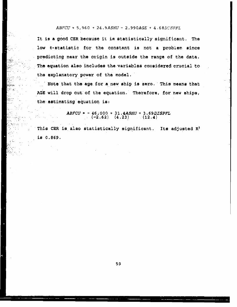
ABFCU = 5,960 + 24.9ASHU - 2,990AGE + 4.68D!SPFL
It is a good CER because it is statistically significant. The
low t-statistic for the constant is not a problem since
predicting near the origin is outside the range of the data.
The+ equation also includes the+ variables considered crucial to
the explanatory power of the model.
Note that the age. for a new ship is zero. This means that
AGE will drop out of the equation. Therefore, for new ships,
the estimating equation is:
ABFCU - 46,000 + 31.4ASHU + 3.69DISPFL(-2.62) (4.23) (12.4)
This CER is also statistically significant. Its adjusted R2
"is 0.869.
59
IV. CONCLUSIONS AND RZCONKENIDATZONS
The two objectives of this thesis were to develop
estimating relationships for both missile EMD costs and
warship fuel consumption. The results of each analysis were
summarized in their respective chapters.
For missile EMD costa, no firm conclusions can be drawn
from the results. Due to the data not being consistent nor
comparable, no statistically significant results were
obtained. Therefore, no significant physical or technical
factors could be identified. However, the coefficients of
variation obtained were much better than the standard factors'
coefficients of variation. This means that the developed CERs
may be a better predictor than the standard factors currently
in use. As long as the NCA analyst realizes their
limitations, the CERs obtained may be helpful in independent
cost analysis.
The recommendation for the missile EMD costs is to do a
follow-on study of this area after the data has been
sanitized. In the meantime, the developed CERs may be useful
since their coefficients of variation are smaller that the
standard factors in use now,
For warship fuel consumptiun, three CERs met the criteria.
The one with the fewest independent variables was chosen as
the best CER. The variables from the best CER were regressed
again, this time using a heteroscedasticity consistent
covariance matrix to remove the effects of heteroscedasticity.
The result was statistically significant and should be of
great help in predicting fuel consumption for inclusion in the
O&S cost estimate. The physical and performance
characteristics identified are steaming hours, age and full
load displacement. Since the age of a new ship is zero, it
will drop out of the equation. A new CER, reflecting the
absence of AGE, was developed and corrected foz
"heteroscedasticity. It was also significant. It is important
that this CER only be used to predict fuel consumption for
ships whose characteristics are similar to those in the data
base, Otherwise, it may not predict fuel consumption with the
accuracy expected.
The recommendations for the fuel consumption section is to
expand the analysis to other ship categories. It appears that
this methodology produces good results and can be applied to
other ship categories.
61
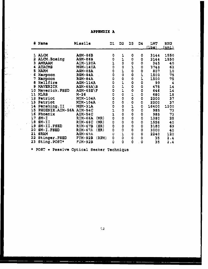
APPENDIX A
# Name Missile D1 D2 D3 D4 LWT RNG.ibs) (nmi)
.1 ALCM AGM-86B 0 1 0 0 3144 15502 ALCMBoeing AGM-86B 0 1 0 0 3144 15503 AMRAAM AIM-120A 1 0 0 0 345 404 ATACMS MGM-140A 0 0 1 0 3748 62S5HARM AGM-88A 0 1 0 0 807 I06 Harpoon RGM-84A 0 0 0 1 1500 757 Harpoon RGM-84A 0 0 0 1 1500 758 Hellfire AGM-114A 0 1 0 0 99 49 MAVERICK AGM-65A\B 0 1 0 0 475 14
2.0 Maverick,FSED AGM-65E\F 0 1 0 0 646 1411 MLRS M-26 0 0 1 0 680 1812 Patriot MIM-104A 0 0 0 0 2200 37213 Patriot MIM-104A 0 0 0 0 2200 37214 Pershing.II MGM-31A 0 0 1 0 16400 1200215 PHOENIX.AIM-56A AIM-54C 1 0 0 0 985 7316 Phoenix AIM-54C 1 0 0 0 985 7317 SM-I RIM-66A (MR) 0 0 0 0 1380 25218 SM-I1 RIM-66C (MR) 0 0 0 0 1556 4019 SM-II.FSED RIM-67B (ER) 0 0 0 0 3180 6920 SM-I.FSED RIM-67A (ER) 0 0 0 0 3000 4021 SRAM AGM-69A U 1 0 0 2240 12022 Stinger.FSED PIM-92B (RPM) 0 0 0 0 35 2.423 Sting.POST* PIM-92B 0 0 0 0 35 2.4
* POST a Passive Optical Seeker Technique
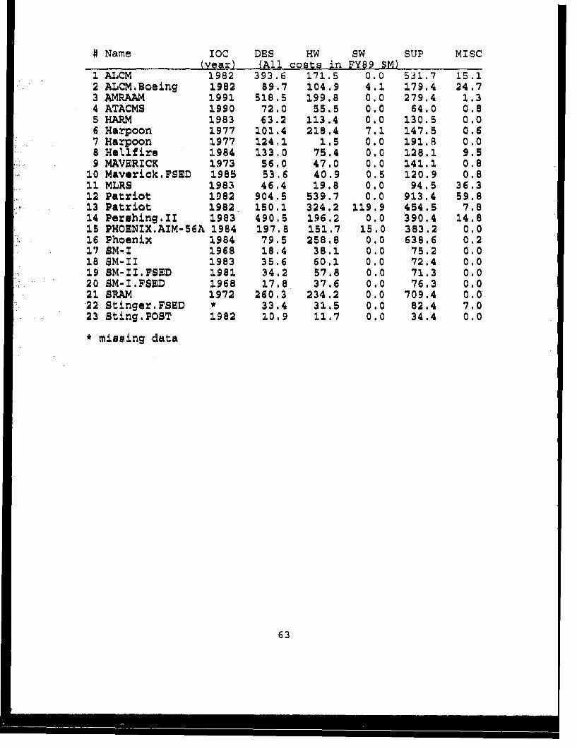
# Name IOC DES HW SW SUP MISC(year) (All costs in PY89 SM)
1 ALCM 1982 393.6 171.5 0.0 531,7 15.12 ALiCM.Boeing 1982 89.7 104.9 4.1 179.4 24.73 AMRAAM 1991 518.5 199.8 0.0 279.4 1.34 ATACMS 1990 72.0 55.5 0.0 64.0 0.85 HARM 1983 63.2 113.4 0.0 130.5 0.06 Harpoon 1977 101.4 218.4 7.1 147.5 0.67 Harpoon 1977 124.1 1.5 0.0 191.8 0.08 Hellfire 1984 133.0 75.4 0.0 128.1 9.59 MAVERICK 1973 56.0 47.0 0.0 141.1 0.8
10 Maverick.FSED 1985 53.6 40.9 0.5 120.9 0.811 MLRS 1983 46.4 19.8 0.0 94.5 36.312 Patriot 1982 904.5 539.7 0.0 913.4 59.813 Patriot 1982 150.1 324.2 119.9 454.5 7,814 Pershing.II 1983 490.5 196.2 0.0 390.4 14.815 PHOENIX.AIM-56A 1984 197.8 151 7 15.0 383.2 0.016 Phoenix 1984 79.5 258.8 0.0 638.6 0.217? SM-I 1968 18.4 38.1. 0.0 75.2 01018 SM-I1 1983 35.6 60.1 0.0 72.4 0.019 SM-II.FSED 1981 34.2 57.8 0.0 71.3 0.020 SM-I.FSED 1968 17.8 37,6 0.0 76.3 0.0
21 SRAM 1972 260.3 234.2 0.0 709.4 0.022 Stinger.FSED * 33.4 31.5 0.0 82.4 7.023 Sting.POST 1982 10.9 11.7 0.0 34.4 010
* missing data
63
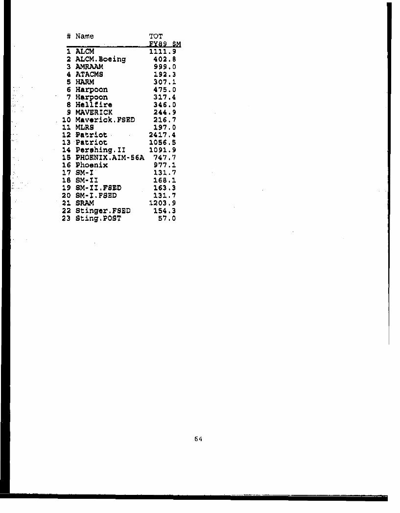
# Name TOTFY89 SM
I ALCM 1111.92 ALCM.Boeing 402.83 AMRAAM 999.04 ATACMS 192.35 HARM 307.16 Harpoon 475.07 Harpoon 317.48 Hellfire 346.09 MAVERICK 244.9
10 Maverick.1'SED 216.711 MLRS 197.012 Patriot 2417.413 Patriot 1056.514 Pershing.II 1091.915 PHOENIX.AIM-56A 747.716 Phoenix 977.117 SM-I 131.718 SM-Il 168.119 SM-II.FSED 163.320 SM-I.FSED 131.721 SRAM 1203.922 Stinger.FSED 154.323 Sting,POST 57.0
64
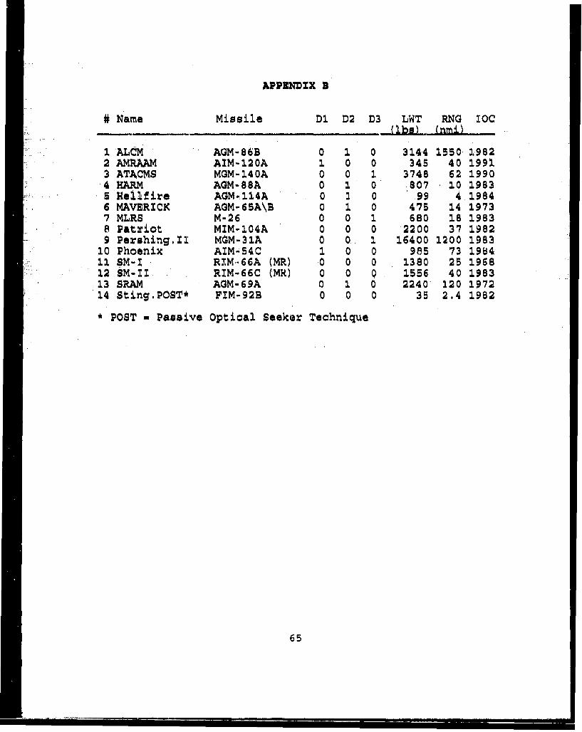
APPENDZX B
# Name Missile D1 D2 D3 LWT RNG IOC•,,,..... ............. (112s ) (nmi),
I. ALCM AGM-86B 0 1 0 3144 ISSO 19822 AMRAAM AIM-120A 1. 0 0 345 40 1991.3 ATACMS MGM-140A 0 0 2 3748 62 19904 HARM AGM-SSA 0 1 0 807 10 19835 Hellfire AGM-.114A 0 0 99 4 19846 MAVERICK AGM-65A\B 0 1 0 475 14 19737 MLRS M-26 0 0 1 680 18 19838 Patriot MIM-104A 0 0 0 2200 37 19829 Pershing. z MGM-31A 0 0 1 16400 1200 1983
10 Phoenix AIM-54C 1 0 0 985 73 198411 SM-I RIM*..66A (MR) 0 0 0 1380 25 196812 SM-11 RIM-66C (MR) 0 0 0 1556 40 198313 SRAM AGM-69A 0 1 0 2240 120 197214 Sting.POST* FIM-92B 0 0 0 35 2.4 1982
* POST - Passive Optical Seeker Technique
65
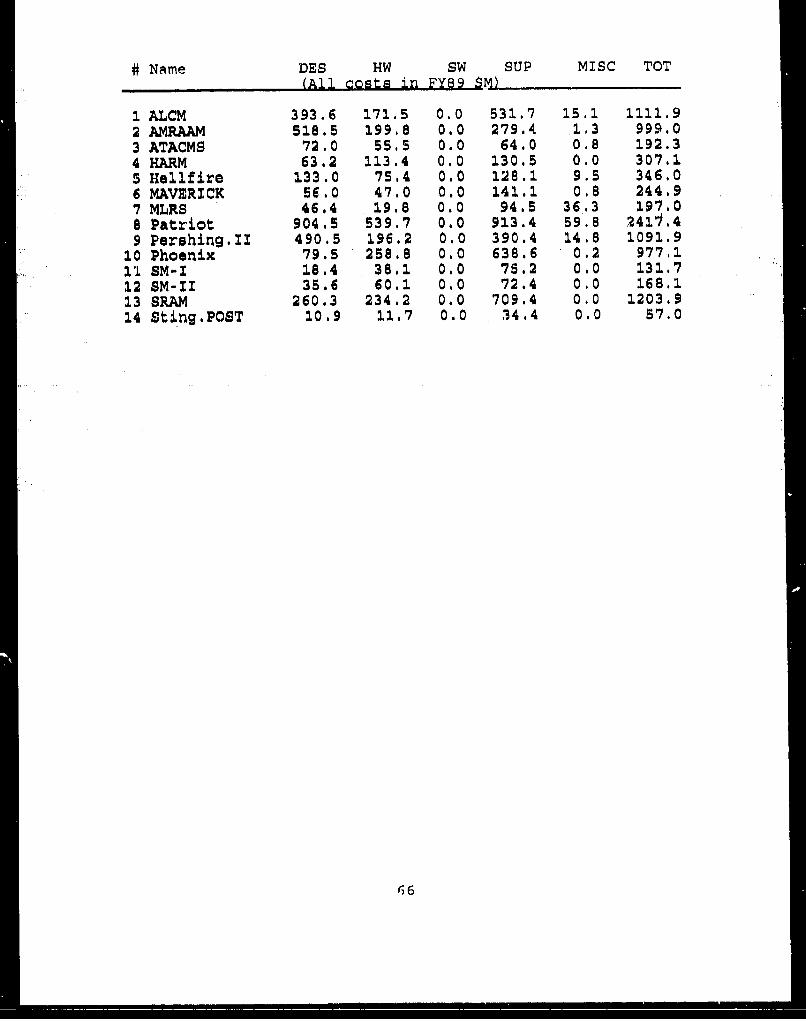
# Name DES NW SW SUP MISC TOT(All costs in FY89 SM)
1 ALCM 393.6 171.5 0.0 531.7 15.1 1111.92 AMRAAM 518.5 199.8 0.0 279.4 1.3 999.03 ATACMS 72.0 55.5 0.0 64.0 0.8 192.34 HARM 63.2 113.4 0.0 130.5 0.0 307.15 Hellfire 133.0 75.4 0.0 128.1 9.5 346.06 MAVERICK 56.0 47.0 0.0 141.1 0.8 244.97 MLRS 46.4 19.8 0.0 94.5 36.3 197.0a Patriot 904.5 539.7 0.0 913.4 59.8 241 .49 Pershing.II 490,5 196.2 0.0 390.4 14.8 1091.9
10 Phoenix 79.5 258.8 0.0 638.6 0.2 977,111. SM-I 18.4 38.1 0.0 75.2 0.0 131.712 SM-I1 35.6 60.1 0.0 72.4 0.0 168.113 SRAM 260.3 234.2 0.0 709.4 0.0 1203,914 Sting.POST 10.9 11.7 0.0 34.4 0.0 57.0
r6
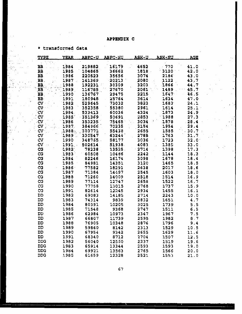
APPENDZX C
"* transformed data
"TYPE YEAR ABFC-U ABFC-b•U . AEH--U. ASH-NU AGE
,E 19184 219882 16179 4652 770 41.0""BB 1'985 104865 361662 1818 3120 ,42.0BB 1986 220523 35656 3074 2184 43.0
..B. 1987 141369 2Q213 2080 1122 43,7B3 1988 192231 30109. 3203 1866 44.7B3 1989 '116785.. 27670 2061 1489 45.7
"1•9'90 136767 29475 2215 1*647 '6. 5BB. 1991 18.0948 25764 3614 1634 47.0
V1982 52945 73032 3823 1683' 24.1CV. 1983 352358 55380 2961 1614 25.1
i"CV 1984. 533413 60036 4324 1873 24. 9"CV 1985" 351369 50691 2853 1988 27.3'CV 1986 353235 7t465 3034 1878 28.4CV 1997 384966 70235 3154. 1954 29.4cv 1988., a,.,.303771, 55438 2655 1585 30.7CV 1989 3305'47 63244 278t 17.63 31.7CV 1.990 3487S5. 58177 3036 1723 32.0CV 1991. 502614- 51938 4083 138' 33.0Co .1982, 78238 13525 2714 1398 17.3co 19-83 60508 10486 2242 1144 18.'3"Ca 1984 8224.6 16174 3098 1678 18.4cO 1985 84981 14351 3120 1465 18.5CO 1986 77582 18291 2638 2017 18.6Ca 1987 71384 14497 2545 1603 18.0co 1988 71260 14009 2518 2514 16.9Ca 1989 77114 12747 2658 1522 16.7CG 1990 77758 13015 2768 1737 1519CG 1991 82614 12245 2934 1455 16.1DD 1982 69083 1.4185 2714 2243 i0.0DD 1983 74314 9839 2832 1651 4.7DD 1984 80391 10205 3025 1739 5.5DD 1985 71548 9368 2747 1511 6.5DT) 1986 62984 10973 2347 1967 7.5DD 1987 66807 11739 2595 1982 8,7DD 1988 76905 10348 2876 1796 9.4DD 1989 59860 8142 2313 1529 10.5DD 1990 67954 9342 2655 1629 1. 6DD 1.991 68340 8712 2704 1507 12.5DDG 1982 56040 12550 2237 1519 19.6DDG 1983 65914 13344 2593 1593 19.0DDG 1984 69921 13563 2765 1566 20.0DDG 1.985 61659 12328 2521 1553 21.0
67
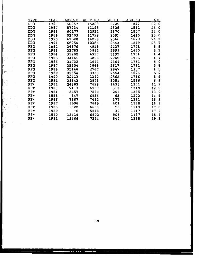
TYPE YEAR ABFC-U ABFC-NU ASH-U ASH-NU AGE,DDG 1986 56257 15220 2220 1842 22.0DDG 1987 57234 13195 2329 1512 23.0DDG 1988 60177 12921 2370 1507 24.0DDG 1989 521593 11799 2091 3.416 25.0DDG 1990 61528 14298 2566 1679 26.3DDO 1991 65754 10386 2643 1219 23.7FFG 1982 34376 4919 2437 1778 5.8FFP 1983 33783 3882 2599 1670 5.1FFP 1984 39902 4397 3192 1754 4.4FF0 1985 34161 3805 2745 1765 4.7FFG 1986 31732 3691 2369 1781 5.0FFG 1987 35204 3868 2617 1792 5.8FF0 1988 35446 2767 2847 1367 4.5FFG 1989 32354 3363 2654 1521 5.2FF0 1990 32413 3342 2562 1746 5.9FFG 1991 38343 2873 3051 1536 6.9FF* 1982 24383 7628 1435 1301 11.9FF* 1983 7413 6937 511 1310 12.9FF* 1984 3157 7280 241 1335 13.9
SFF* 1985 847 6936 65 1270 14.91F* 3.986 7367 7452 377 1311 15. 9
SFP* 1987 5596 7645 401 1338 16.9"FF* 1988 -320 6653 56 1219 17.6FF* 1989 -6 5818 32 1117 17.9FF* 1990 13414 6602 906 1197 18.9FF* 1991 12466 7244 840 1318 19.5
68
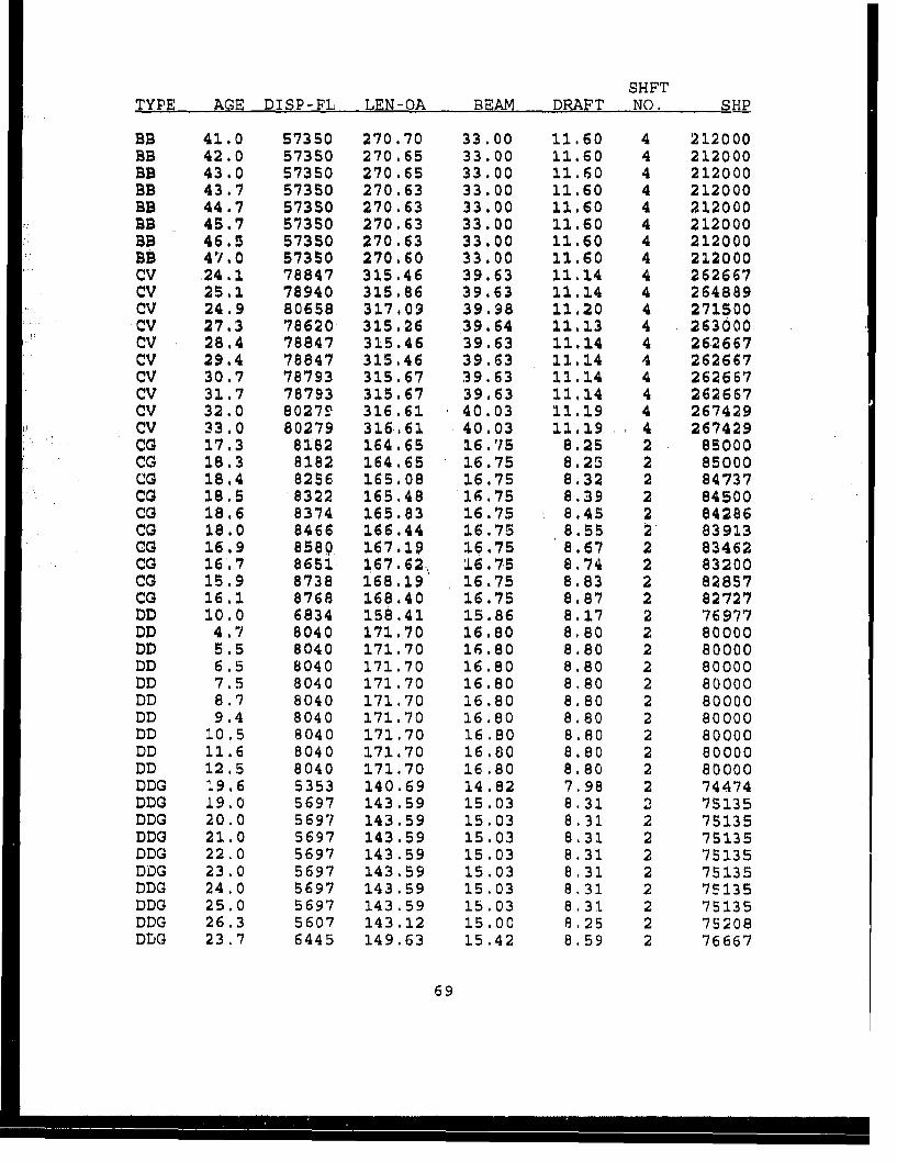
SHFTTYPE AGE DISP-FL LEN-OA BEAM DRAFT NO. SHP
BB 41.0 57350 270.70 33.00 11.60 4 212000BB 42.0 57350 270.65 33.00 11.60 4 212000BB 43.0 57350 270.65 33.00 11.60 4 212000BB 43.7 57350 270.63 33.00 11.60 4 212000BS 44.7 57350 270.63 33.00 11.60 4 212000a 45.7 57350 270.63 33.00 11.60 4 212000BB 46.5 57350 270.63 33.00 11.60 4 212000aBs 47.0 57350 270.60 33.00 11.60 4 212000CV 24.1 78847 315.46 39.63 11.14 4 262667CV 25.1 78940 315.86 39.63 11.14 4 264889CV 24.9 80658 317.09 39.98 11.20 4 271500CV 27.3 78620 315.26 39.64 11.13 4 263000CV 28.4 78847 315.46 39.63 11.14 4 262667CV 29.4 78847 315.46 39.63 11.14 4 262667CV 30.7 78793 315.67 39.63 11.14 4 262667CV 31.7 78793 315.67 39.63 11.14 4 262667CV 32.0 80279 316.61 40.03 11.19 4 267429CV 33.0 80279 316,61 40.03 11.19 4 267429Co 17.3 8182 164.65 16 .75 8.25 2 85000CG 18.3 8182 164.65 16.75 8.25 2 85000CG 18.4 8256 165.08 16.75 8.32 2 84737Co 18.5 8322 165.48 16.75 8.39 2 84500Co 18.6 8374 165.83 16.75 8.45 2 84286Co 18.0 8466 166.44 16.75 8.55 2 83913CG 16.9 8580 167.19 16.75 8.67 2 83462Co 16.7 8651 167.62., 16.75 8.74 2 83200Ca 15.9 8738 168.19 16.75 8.83 2 82857Ca 16.1 8768 168.40 16.75 8.87 2 82727DD 10.0 6834 158.41 15.86 8.17 2 76977DD 4.7 8040 171.70 16.80 8.80 2 80000DD 5.5 8040 171.70 16.80 8.80 2 80000DD 6.5 8040 171.70 16.80 8.80 2 80000DD 7.5 8040 171.70 16.80 8.80 2 80000DD 8.7 8040 171.70 16.80 8.80 2 80000DD 9.4 8040 171.70 16.80 8.80 2 80000DD 10.5 8040 171.70 16.80 8.80 2 80000DD 11.6 8040 171,70 16.80 8.80 2 80000DD 12.5 8040 171.70 16.80 8.80 2 80000DDG 19.6 5353 140.69 14.82 7.98 2 74474DDG 19.0 5697 143.59 15.03 8.31 2 75135DDG 20.0 5697 143.59 15.03 8.31 2 75135DDG 21.0 5697 143.59 15.03 8.31 2 75135DDG 22.0 5697 143.59 15.03 8.31 2 75135DDG 23.0 5697 143.59 15.03 8.31 2 75135DDG 24.0 5697 143.59 15.03 8.31 2 75135DDG 25.0 5697 143.59 15.03 8.31 2 75135DDG 26.3 5607 143.12 15.00 8.25 2 75208DDG 23 .7 6445 149.63 15.42 8.59 2 76667
69
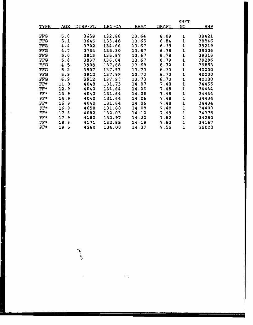
SIFTTYPE AGE DISP-FL LEN-OA BEAM DRAFT NO. SHP
FFG 5.8 3658 132.86 13.64 6.89 1 38421FFG 5.1 3645 133.48 13.65 6.84 1 38846FFG 4.4 3702 134.66 13.67 6.79 1 39219FFG 4.7 3754 135.30 13.67 6.78 1 39306FFG 5.0 3813 135.87 13.67 6.78 1 39318FFG 5.8 3837 136.04 13.67 6.79 1 39286FFG 4.5 3908 137.68 13.69 6.72 1 39853FFG 5.2 3907 137.93 13.70 6.70 1 40000FFG 5.9 3912 137.98 13.70 6.70 1 40000FFQ 6.9 3912 137,97 13.70 6.70 1 40000FF* 11.9 4048 131.73 14.07 '7.48 1 34455FF* 12.9 4040 131.64 14.06 7.48 1 34434FF* 13.9 4040 131.64 14.06 7.48 1 34434FF* 14.9 4040 131.64 14.06 7.48 1 34434FF* 15.9 4040 131.64 14.06 7.48 1 34434FF* 16.9 4058 131.80 14.08 7.48 1 34400FF* 17.6 4082 132.03 14.10 7.49 1 34375FF* 17.9 4180 132.97 14.20 7.52 1 34250FF* 18.9 4171 132.85 14.19 7.52 1 34167FF* 19.5 4260 134.00 14.30 7.55 1 35000
_____________________________
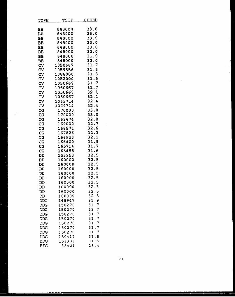
TYPE TSHP SPEED
BE 848000 33.0BE 848000 33.0BE 848000 33.0BB 848000 33.0BE 848000 33.0BE 848000 33.0BE 848000 3:.0BE 848000 33.0CV 1050667 31.7CV 1059556 31.8CV 1086000 31.8CV 1052000 31.5CV 1050667 31.7CV 1050667 31.7CV 1050667 32.1CV 1050667 32.1CV 1069714 32.4CV 1069714 32.4CG 170000 33.0CG 170000 33.0CG 169474 32.8CG 169000 32.7CG 168571 32.6CG 167826 32.3CG 166923 32.1CG 166400 31.9CG 165714 31.7CG 165455 31.6DD 153953 32.5DO 160000 32.5DD 160000 32.5DD 160000 32.5DD 160000 32.5DD 160000 32.5DD 160000 32.5DD 160000 32.5DD 160000 32.5DD 160000 32.5DOG 148947 31.9DDG 150270 31.7DDG 150270 31.7DDG 150270 31.7DDG 150270 31.7DDG 150270 31.7DDG 150270 31.7DDG 150270 31.7DDG 150417 31.8DUG 153333 31.5FFG 38421 28.4
71
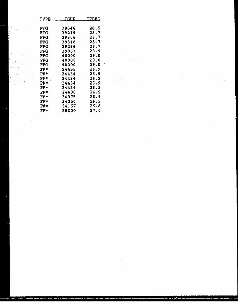
TE .. TSHP SPEED
FFG 38846 28.5FFG 39219 28.7FFG 39306 28.7FFG 39318 28.7FFG 39286 28.7FFG 39853 28.9FFG 40000 29.0V'FG 40000 29.0
"FP 40000 29.0FF* 34455 26.9FF* 34434 26.9FF* 34434 26. 9FF* 34434 26.9FF* 34434 26.9FF* 34400 26.9FF* 34375 26.9FF* 34250 26.9FF* 34167 26.8FF* 35000 27.0
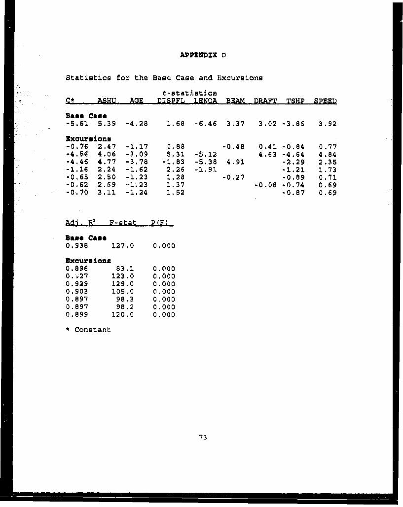
APPENDIX D
Statistics for the Base Case and Excursions
C* ASHU AGE DISPFL LENQA BEAM DRAFT TSHP SPEED
Base Came-5.61 5.39 -4.28 1.68 -6.46 3.37 3.02 -3.86 3.92
Excurs ions-0.76 2.47 -1.17 0.88 -0.48 0.41 -0.84 0.77-4.56 4.06 -3.09 5.31 -5.12 4.63 -4.64 4.84-4.46 4.77 -3.78 -1.83 -5.38 4.91 -2.29 2.35-1.16 2.24 -1.62 2.26 -1.91 -1.21 1.73-0.65 2.50 -1.23 1.28 -0.27 -0.89 0.71-0.62 2.69 -1.23 1.37 -0.08 -0.74 0.69-0.70 3.11 -1.24 1.52 -0.87 0.69
Adj. R2 F-stat P(F)
Bass Case0.938 127.0 0.000
Excursions0.896 83.1 0,0000.-127 123.0 0.0000.929 129.0 0.0000.903 105.0 0.0000.897 98.3 0.0000.897 98.2 0.0000.899 120.0 0.000
* Constant
73
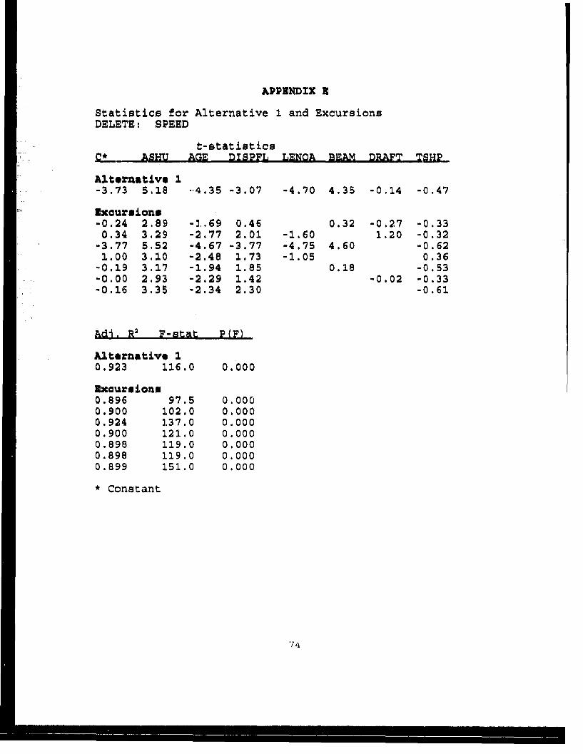
APPENDIX E
Statistics for Alternative I and ExcursionsDELETE: SPEED
t-statistics_,. &ASHU AGE DISPFL LENOA BEAM DRAFT TSHP-
Alternative .-3.73 5.18 --4.35 -3.07 -4.70 4.35 -0.14 -0.47
"Exoursions-0.24 2.89 -1.69 0.46 0.32 -0.27 -0.330.34 3.29 -2.77 2.01 -1.60 1.20 -0.32
"-3.77 5.52 -4.67 -3.77 -4.75 4.60 -0 .621.00 3.10 -2.48 1.73 -1.05 0.36
-0.19 3.17 -1.94 1.85 0.18 -0.53-0.00 2.93 -2.29 1.42 -0.02 -0.33-0.16 3.35 -2.34 2.30 -0.61
Adj. RI F-stat P(F)
Alternative 10.923 116.0 0.000
Exaursions0.896 97.5 0.0000.900 102.0 0.0000.924 137.0 0.0000.900 121.0 0.0000.898 119.0 0.0000.898 119.0 0.0000.899 151.0 0.000
* Constant
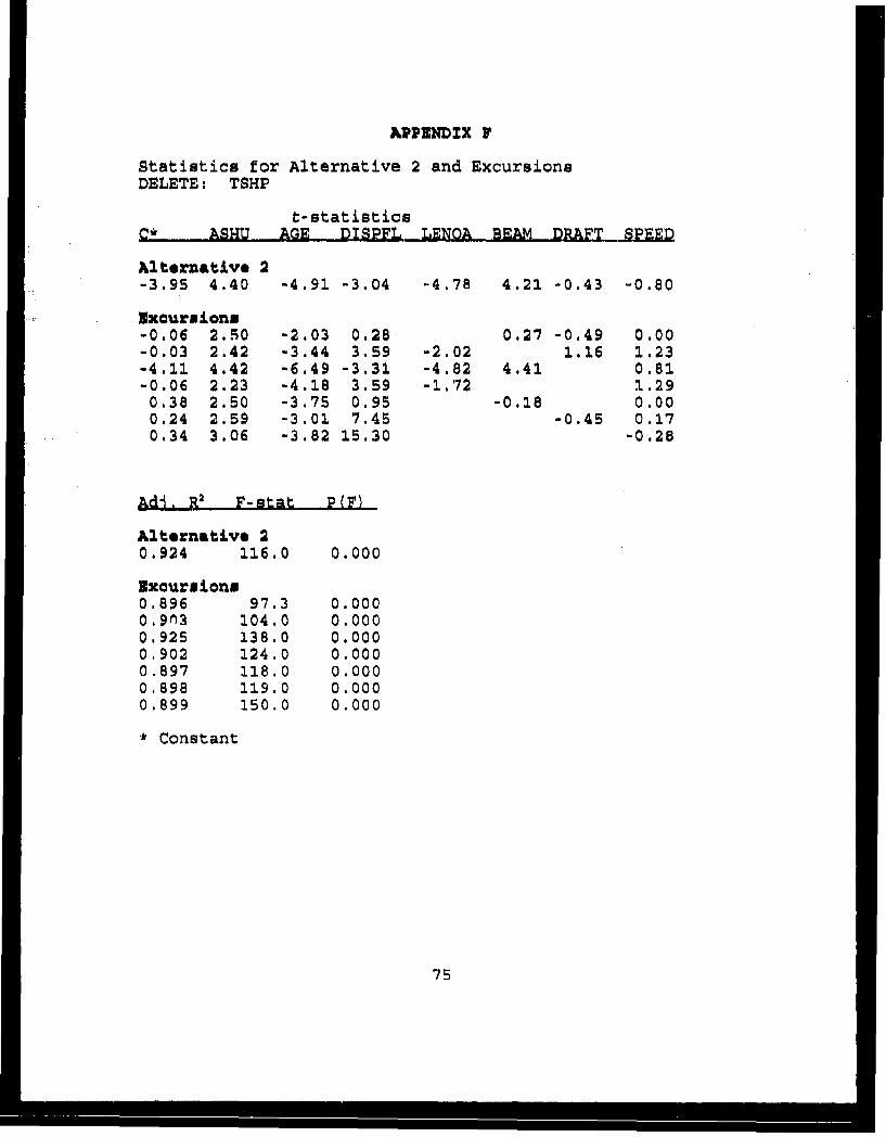
APPZNDZX F
Statistics for Alternative 2 and ExcursionsDELETE: TSHP
t-statisticsC* ASHTJ AGE DISPFL LENOA BEAM DRAFT -PEED
Alternative 2-3.95 4.40 -4.91 -3.04 -4.78 4.21 -0.43 -0.80
3xoursions-0.06 2.50 -2.03 0.28 0.27 -0.49 0.00-0.03 2.42 -3.44 3.59 -2.02 1.16 1.23-4.11 4.42 -6.49 -3.31 -4.82 4.41 0.81-0.06 2.23 -4.18 3.59 -1.72 1.290.38 2.50 -3.75 0.95 -0.18 0.000.24 2.59 -3.01 7.45 -0.45 0.170.34 3.06 -3.82 15.30 -0.28
Ad-. R2 F-stat P(F)
Alternative 20.924 116.0 0.000
Excursions0.896 97.3 0.0000.9n3 104.0 0.0000.925 138.0 0.0000.902 124.0 0.0000.897 118.0 0.0000.898 119.0 0.0000.899 150.0 0.000
* Constant
75
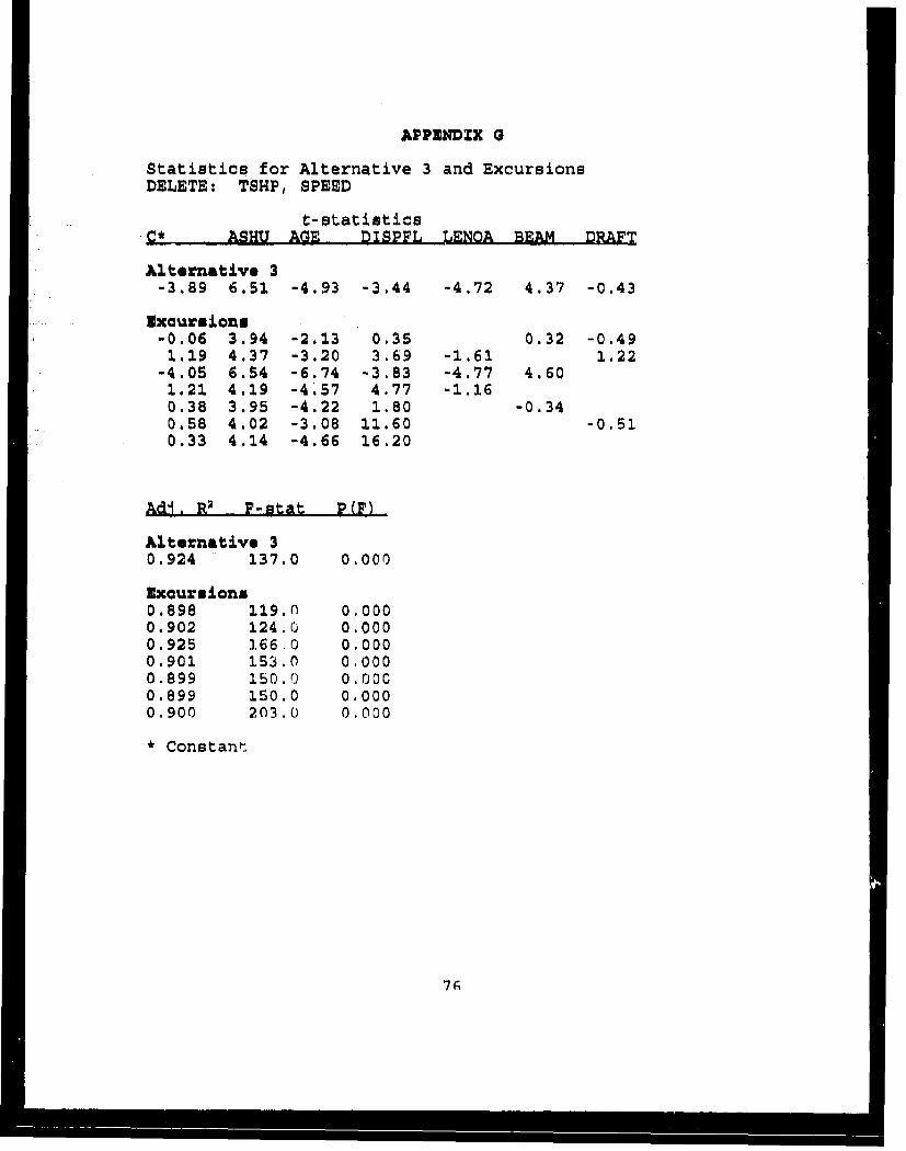
APPENDZX a
Statistics for Alternative 3 and ExcursionsDELETE: TSHP, SPEED
t-statisticsASHU AGE DISPFL LENOA BEAM DRAFT
Alternative 3-3.89 6.51 -4.93 -3.44 -4.72 4.37 -0.43
Zxcursions-0.06 3.94 -2.13 0.35 0.32 -0.491.19 4.37 -3.20 3.69 -1.61 1.22
-4.05 6.54 -6.74 -3.83 -4.77 4.601.21 4.19 -4.57 4.77 -1.160.38 3.95 -4.22 1.80 -0.340.58 4.02 -3.08 11.60 -0.510.33 4.14 -4.66 16.20
Adj. R2 P-stat P(F)
Alternative 30.924 137.0 0.000
Excursions0.898 119.0 0,0000.902 124.0 0.0000.925 166.0 0.0000.901 153.0 0.0000.899 150.o O.OOC0.899 150.0 0.0000.900 203.0 0.000
* Constant
7';
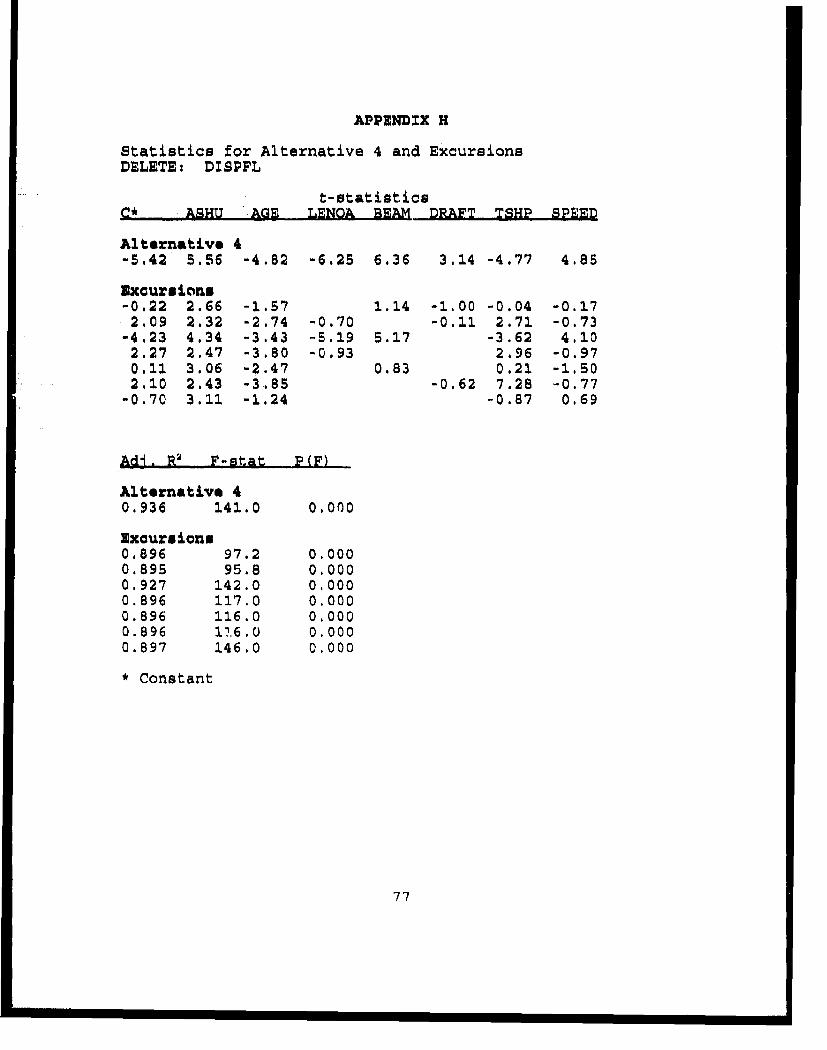
APPENDIX H
Statistics for Alternative 4 and ExcursionsDELETE: DISPFL
t-statisticsQ*_ • ASHU AGE LENOA BEAM DRAFT TSHP SPEED
Alternative 4-5.42 5.56 -4.82 -6.25 6,36 3.14 -4.77 4.85
Excursions-0.22 2.66 -1.57 1.14 -1.00 -0.04 -0.172.09 2.32 -2.74 -0.70 -0.11 2.71 -0.73
-4.23 4.34 -3.43 -5.19 5.17 -3.62 4.102.27 2.47 -3.80 -0.93 2.96 -0.970.11 3.06 -2.47 0.83 0.21 -1.502.10 2.43 -3.85 -0.62 7.28 -0.77
"-0.70 3.11 -1.24 -0.87 0.69
Adl. R2 F-stat R(F)
Alternative 40,936 141.0 0.000
Excursions0.896 97.2 0.0000.895 95.8 0.0000.927 142.0 0.0000.896 117.0 0.0000.896 116.0 0.0000.896 17.6.0 0.0000.897 146.0 0.000
* Constant
77
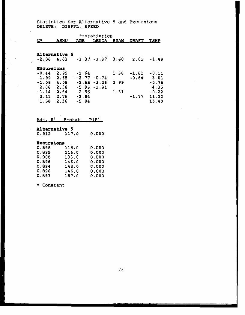
Statistics for Alternative 5 and ExcursionsDELETE: DISPFL, SPEED
t-statisticsC* ASHU AGE LENOA BEAM DRAFT TSHR
Alternative 5-2.06 4.61 -3.37 -3.37 3.60 2.01 -1.48
Exoursions-0.44 2.99 -1.64 1.38 -1.81 -0.111.99 2.65 -2.77 -0.74 -0.64 3.01
-1.08 4.05 -2.65 -3.26 2.99 -0.752.06 2.58 -5.93 -1.81 4.35
-1.14 2.64 -2.56 1.31 -0.222.11 2.76 -3.84 -1.77 11.301.58 2.36 -5.84 15.40
Adi. R2 F-Stat P(F)
Alternative 50.912 117.0 0.000
Excursions0.898 118.0 0.0000.895 116.0 0.0000.908 133.0 0.0000.896 146.0 0.0000.894 142.0 0.0000.896 146.0 0.0000.893 187.0 0.000
• Constant
i1
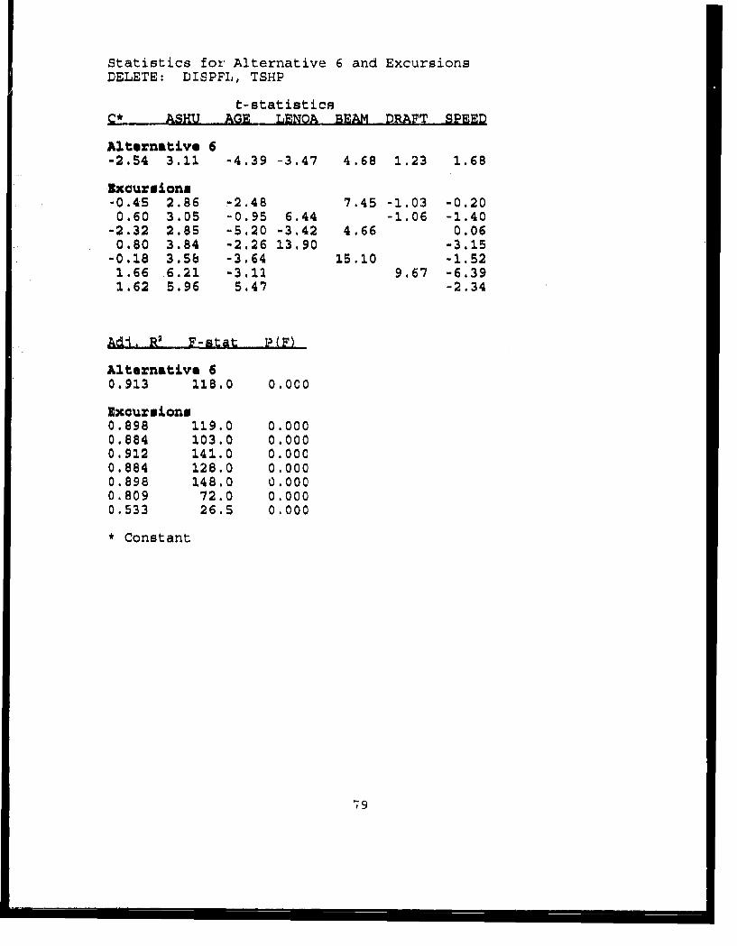
Statistics for Alternative 6 and ExcursionsDELETE: DISPFL, TSHP
t-statisticsASHU AGE LENO..A EAM DRAFT SPEED
Alternative 6-2.54 3.11 -4.39 -3.47 4.68 1.23 1.68
Zxcursions-0.45 2.86 -2.48 7.45 -1.03 -0.200.60 3.05 -0.95 6.44 -1.06 -1.40
-2.32 2.85 -5.20 -3.42 4.66 0.060.80 3.84 -2.26 13.90 -3.15
-0.18 3.5b -3.64 15.10 -1.521.66 6.21 -3.11 9.67 -6.391.62 5.96 5.47 -2.34
Adj. R• 2 F-stat P(F)
Alternative 60.913 118.0 0.000
Excursions0.898 119.0 0.0000.884 103.0 0.0000.912 141.0 0.0000.884 128.0 0.0000.898 148.0 0.0000.809 72.0 0.0000.533 26.5 0.000
* Constant
779
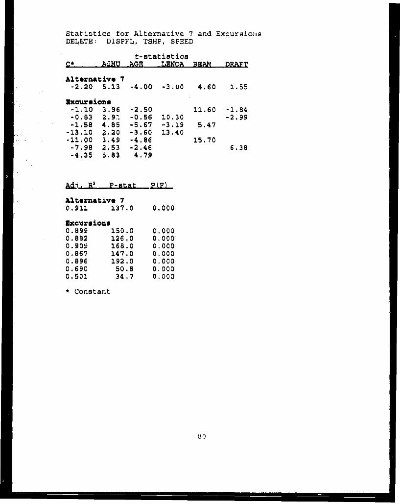
Statistics for Alternative 7 and ExcursionsDELETE: DISPFL, TSHP, SPEED
t-statisticsC* • AJHU AGE LENOA BEAM DRAFT
Alternative 7-2.20 5.13 -4.00 -3.00 4.60 1.55
Excaursions-1.10 3.96 -2.50 11.60 -1.84-0.83 2.91 -0.56 10.30 -2.99-1.58 4.85 -5.67 -3.19 5.47
-13.10 2.20 -3.60 13.40-11.00 3.49 -4.86 15.70-7.98 2.53 -2.46 6.38-4.35 5.83 4.79
R2 F-stat £P(F)
Alternative 70.911 137.0 0.000
LEcursions0.899 150.0 0.0000.882 126.0 0.000,0.909 168.0 0.0000.867 147.0 0.0000.896 192.0 0.0000.690 50.8 0,0000.501 34.7 0.000
* Constant
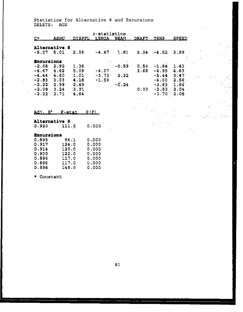
Statistics for Alternative 8 and ExcursionsDELETE: AGE
t-statisticeASHU DISPFL LENOA DRAFT TSHP SPEED
Alteznative 8-5.07 5.01 2.56 -4.47 1.81 2.34 -4.,52 3.99
Exour sions-2.08 2.92 1.36 -0.59 0.54 -1.84 1.43-4.67 4.62 5.09 -4.07 3.68 -4.95 4.63-4.44 4.60 1.01 -3.73 3.32 -5.44 3.47-2.83 3.03 4.18 -1.59 -4.00 2.56-2.22 2.99 2.49 -0.24 -3.63 1.64-2.08 3.24 3.91 0.00 -2.83 2.04-2.33 3.71 4.64 -3.70 2.08
Add. R2 F-stat P(F)
Alternative 80.920 111.0 0.000
Excursions0.895 96.1 0.0000.917 124.0 0.0000.914 120.0 0.0000.900 122.0 0.0000.896 117.0 0.0000.896 117.0 0.0000.898 148.0 0.000
* Constant
81
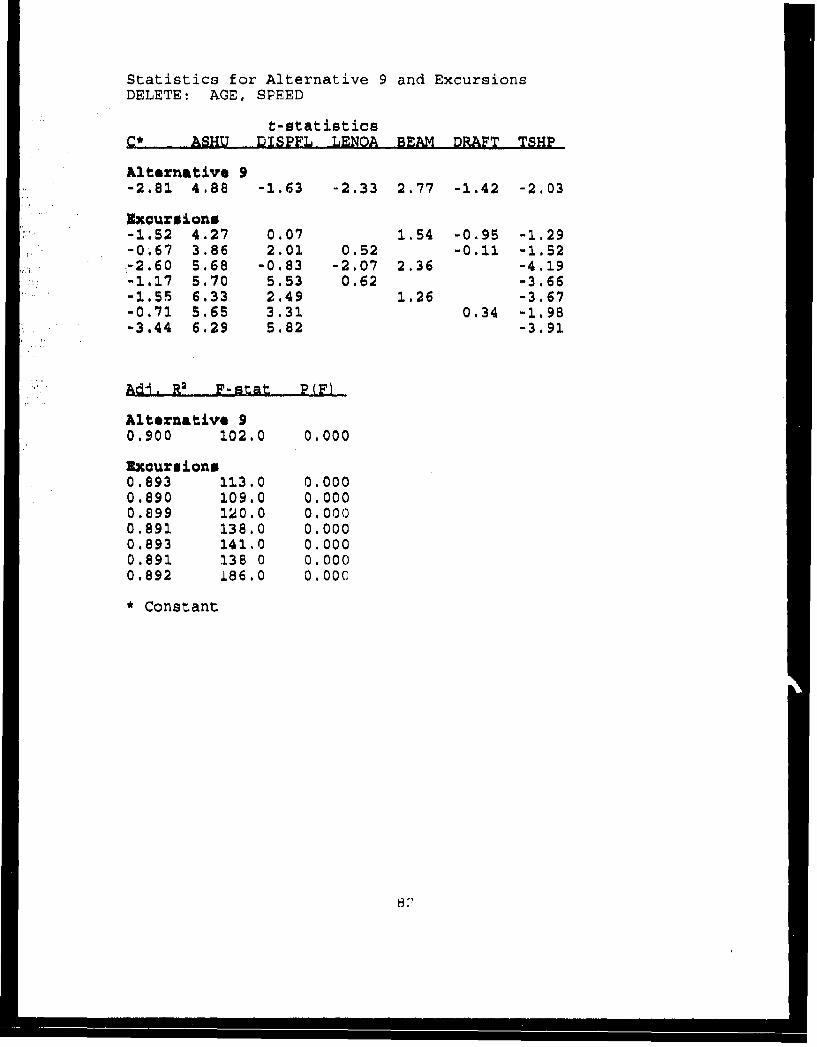
Statistics for Alternative 9 and ExcursionsDELETE: AGE, SPEED
t-statisticsC* . ASHU DISPFL LENOA BEAM DRAFT TSHP
Alterznative 9-2.81 4.88 -1.63 -2.33 2.77 -1.42 -2.03
ExcuZsions-1.52 4.27 0.07 1.54 -0.95 -1.29-0.67 3.86 2.01 0.52 -0.11 -1.52i -2.60 5.68 -0.83 -2.07 2.36 -4.19-1.17 5.70 5.53 0.62 -3.66-1.55 6.33 2.49 1.26 -3.67-0.71 5.65 3.31 0.34 -1.98-3.44 6.29 5.82 -3. 91
Adi. R2 F-stat P(F)
Alternative 90.900 102.0 0.000
Exoursions0.893 113.0 0.0000.890 109.0 0.0000.899 120.0 0.0000.891 138.0 0.0000.893 141.0 0.0000.891 138 0 0.0000.892 186.0 0.000
* Constant
8 ;
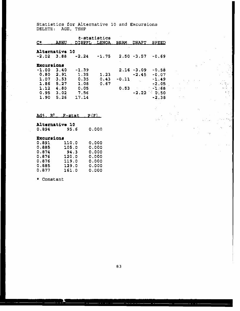
Statistics for Alternative 10 and ExcursionsDELETE: AGE, TSHP
t-statisticsC* •ASHU DISPFL LENOA BEAM DRAFT SPEED
Alternative 10-2.02 3.88 -2.24 -1.75 2.50 -3.57 -0.69
Excuzrions-1.00 3.40 -1.39 2.16 -3.09 -0.580.80 2.91 1.35 1.23 -2.45 -0.071.07 3.53 0.35 0.43 -0.11 -1.491.86 5.27 1.08 0.67 -2.051.12 4.80 0.05 0.53 -1;680.95 3.02 7.56 -2.22' 0.50 S1.90 5.26 17.14 -2.38
Adj. R2 F_-stat P(F)
Alternative 100.894 95,6 0.000
Excursions0.891 110.0 0,0000.885 105.0 0.0000.874 94.3 0.0000.876 120.0 0.0000.876 119.0 0.0000.885 129.0 0.0000.877 161.0 0.000
* Constant
83
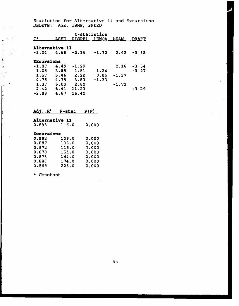
Statistics for Alternative 11 and ExcursionsDELETE: AGE, TSHP, SPEED
t-statisticsC* ASHU DISPFL LENOA BEAM DRAFT
Alternative 11-2.04 4.66 -2.14 -1.72 2.42 -3.88
Excursions-1.07 4.49 -1.29 2.16 -3.541.05 3.85 1.81 1.34 -3.271.57 3.46 2.22 0.85 -1.370.75 4.75 3.83 -1.331.37 5.03 2.80 -1.732.42 5.41 11.23 -3.29
-2.88 4.67 16.40
AdA. R2 F-stat P(F)
Alternative 110.895 116.0 0.000
Excursions0.892 139.0 0.0000.887 133.0 0.0000.872 115.0 0.0000.870 151.0 0.0000.873 154.0 0.0000.886 174.0 0.0000.869 223.0 0.000
* Constant
8 4
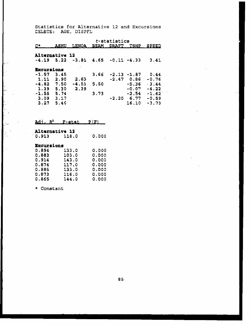
Statistics for Alternative 12 and ExcursionsDELETE: AGE, DISPFL
t-statisticsC* & ASHU LENOA BEAM DRAFT TSHP SPEED
Alternative 12-4.19 5.22 -3.81 4.65 -0.11 -4.33 3.41
Exc•rmions-1.57 3.45 3.66 -2.13 -1.87 0.441.11 2.90 2.63 -2.47 0.86 -0.76
-4.82 7.50 -4.51 5.50 -5.36 3.441.39 5.30 2.39 -0.07 -4.22
-1.55 5.74 3.73 -2.54 -1.623.09 3.17 -2.20 6.77 -0.593.27 5.4G 16.10 -3.73
Adj. R2 F-stat P(F)
Alternative 120.913 118.0 0.000
Excursions0.894 133.0 0.0000.883 103.0 0.0000.914 143.0 0.0000.874 117.0 0.0000.886 133.0 0.0000.873 116.0 0.0000.865 144.0 0.000
* Constant
85
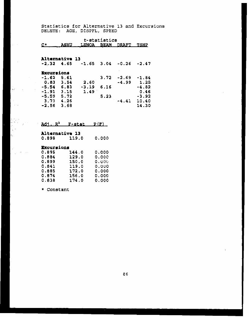
Statistics for Alternative 13 and ExcursionsDELETE: AGE, DISPFL, SPEED
t-statisticsCk ASNU LENOA BEAM DRAFT TSHP
Alternative 13-2.32 4.65 -1.65 3.04 -0.26 -2.47
Excursions-1.62 5.61 3.72 -2.69 -1.840.83 3.54 2.60 -4.99 1.25
-5.54 6.83 -3.19 6.16 -4.82-1.91 3.15 1.49 0.46-5.59 5.72 5.23 -3.923.73 4.26 -4.41 10.40
-2.56 3.68 14.30
Ad., Rg F-stat P(F)
Alternativa 130.898 119.0 0.000
Exoursions0.895 144.0 0.0000.884 129.0 0.0000.899 150.0 0.0000.841 119.0 0.0000.885 172.0 0.0000.874 156.0 0.0000.838 174.0 0.000
* Constant
86
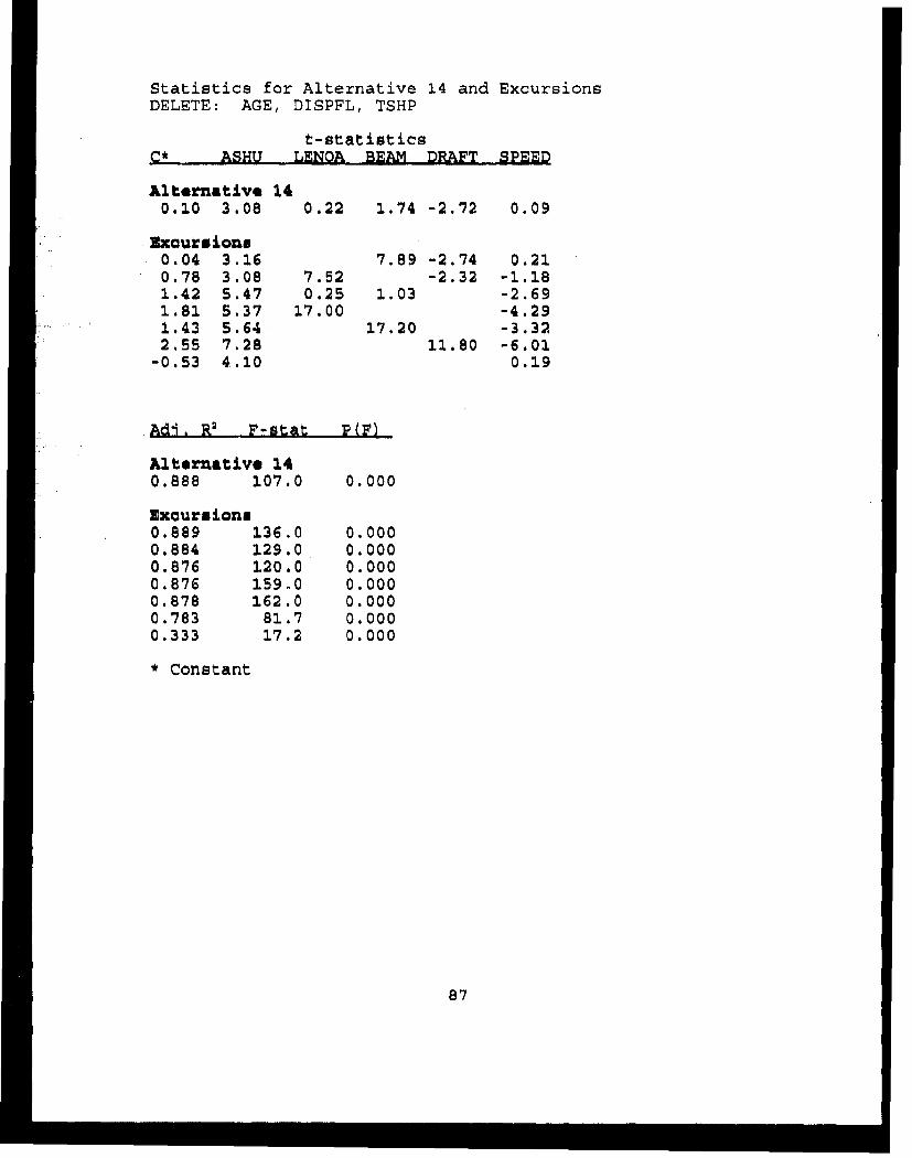
Statistics for Alternative 14 and ExcursionsDELETE: AGE, DISPFL, TSHP
t-statisticsC* ASHU LENOA BEAM DRAFT SPEED
Alternative 140.10 3.08 0.22 1.74 -2.72 0.09
xcaursions0.04 3.16 7.89 -2.74 0.210.78 3.08 7.52 -2.32 -1.181.42 5.47 0.25 1.03 -2.691.81 5.37 17.00 -4.291.43 5.64 17.20 -3.322.55 7.28 11.80 -6.01
-0.53 4.10 0.19
Adi. R2 F-stat P(p)
Alternative 140.888 107.0 0.000
Ixcursions0.889 136.0 0.0000.884 129.0 0.0000.876 120.0 0.0000.876 159.0 0.0000.878 162.0 0.0000.783 81.7 0.0000.333 17.2 0.000
* Constant
87
1 1 1 1 1 1i
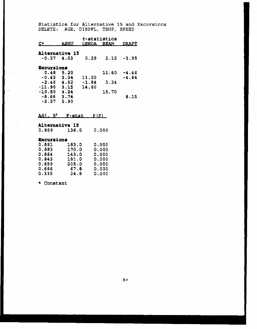
Statistics for Alternative 15 and ExcursionsDELETE: AGE, DISPFL, TSHP, SPEED
t-statisticsC* ASHU LENQA BEAM DRAFT
Alternative 15-0.37 4.03 0.29 2.12 -3.95
Excursions0.48 5.20 11.60 -4.46
-0.62 3.34 11.00 -4.84-2.46 4.62 -1.84 3.34
-11.90 3.15 14.60-10.50 4.24 15.70-8.66 3.74 8.15-2.27 5.90
Ad-i. R2 F-stat P(F)
A1ternative 150.889 136.0 0.000
Excursions0.891 183.0 0.0000.883 170.0 0.0000.864 143.0 0.0000.843 181.0 0.0000.859 205.0 0.0000.666 67.8 0.0000.335 34.8 0.000
* Constant
88
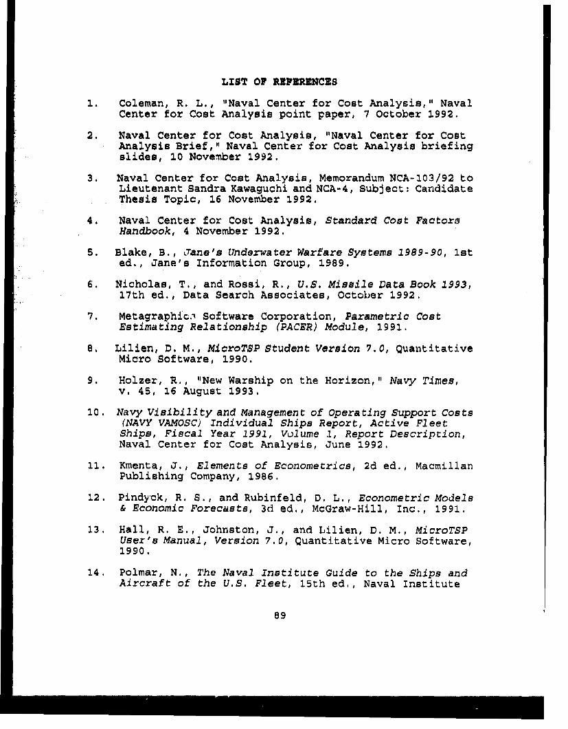
LIST OF REFERENCES
1. Coleman, R. L., "Naval Center for Cost Analysis," NavalCenter for Cost Analysis point paper, 7 October 1992.
2. Naval Center for Cost Analysis, "Naval Center for CostAnalysis Brief," Naval Center for Cost Analysis briefingslides, 10 November 1992.
3. Naval Center for Cost Analysis, Memorandum NCA-103/92 toLieutenant Sandra Kawaguchi and NCA-4, Subject: CandidateThesis Topic, 16 November 1992.
4. Naval Center for Cost Analysis, Standard Cost FactorsHandbook, 4 November 1992.
5. Blake, B., Jane's Underwater Warfare Systems 1989-90, 1sted., Jane's Information Group, 1989.
6. Nicholas, T., and Rossi, R., U.S. Missile Data Book 1993,.17th ed., Data Search Associates, October 1992.
7. Metagraphic.i Software Corporation, Parametric CostEstimating Relationship (PACER) Module, 1991.
8. Lilien, D. M., MicroTSP Student Version 7.0, QuantitativeMicro Software, 1990.
9. Holzer, R., "New Warship on the Horizon," Navy Times,v. 45, 16 August 1993.
10. Navy Visibility and Management of Operating Support Costs(NAVY VAMOSC) Individual Ships Report, Active FleetShips, Fiscal Year 1991, Volume ., Report Description,Naval Center for Cost Analysis, June 1992.
11. Kmenta, J., Elements of Econometrics, 2d ed., MacmillanPublishing Company, 1986.
12. Pindyck, R. S., and Rubinfeld, D. L., Econometric Models& Economic Forecasts, 3d ed., McGraw-Hill, Inc., 1991.
13. Hall, R. E., Johnston, J., and Lilien, D. M., MicroTSPUser's Manual, Version 7.0, Quantitative Micro Software,1990.
14. Polmar, N., The Naval Institute Guide to the Ships andAircraft of the U.S. Fleet, 15th ed., Naval Institute
89
Press, 1993.
15. Polmar, N., The Ships and Aircraft of the U.S. Fleet,12th ed., Naval Institute Press, 1981.
90
INITIAL DISTRIBUTION LIST
No. Copies1. Defense Technioal Information Center 2
Cameron StationAlexandria VA 22304-6145
2. Library, Code 052 2Naval Postgraduate SchoolMonterey CA 93943-5002
3. Professor Dan C. Boger, AS/Bo 2Department of Administrative SciencesNaval Postgraduate SchoolMonterey, CA 93943-5103
4. Professor Michael G. Sovereign, OR/Sm 2Department of Operations ResearchNaval Postgraduate SchoolMonterey, CA 93943-5000
5. Commanding Officer 2Naval Center For Cost AnalysisPentagon, Room 4A538Washington, DC 20350-1100
6. Commanding Officer 5Naval Computer and Telecommunications
Station, WashingtonWashington, D.C. 20374-5069Attn: LT Sandra A. Williams