Embed Size (px)
Citation preview
0NAVAL POSTGRADUATE SCHOOL
Monterey, California
AD-A274 841 DTICIII~l~lM~ • •ELECTFTATr.• JAN 2 51994
THESIS
AN EVALUATION OF A TACTICAL ACTIVEMULTI-ENVIRONMENT ACOUSTIC PREDICTION
SYSTEM VS MEASURED DATA
by
Robert Eric Coleman
September 1993
Thesis Advisor: Micheal J. PastoreSecond reader: Alan B.Coppens
Approved for public release; distribution is unlimited.
94-02096I I~m11141111 l4ll 05lillllli9145
REPORT DOCUMENTATION PAGE Form Approved OMB No.0704-OIU
Public reporting burden for this collection of information is estimated to average I hour per response, including the time for reviewing instruction,searching existing data sources, gathering and maintaining the data needed, and completing and reviewing the collection of information. Send commentsregarding this burden estimate or any other aspect of this collection of information, including suggestions for reducing this burden, to Washingonheadquarters Services, Directorate for Information Operations and Reports, 1215 Jefferson Davis Highway, Suite 1204, Arlington. VA 22202-4302, andto the Office of Management and Budget. Paperwork Reduction Project (0704-0188) Washington DC 20503.
1. AGENCY USE ONLY (Leave blank) 2. REPORT DATE 3.REPORT TYPE AND DATES COVEREDSeptember 1993 Master's Thesis
4. TITLE AND SUBTITLE 5. FUNDING NUMBERS
AN EVALUATION OF A TACTICAL ACTIVE MULTI-ENVIRONMENT ACOUSTIC PREDICTION SYSTEM VSMEASURED DATA
6. AUTHOR(S)
Coleman, Robert Eric
7. PERFORMING ORGANIZATION NAME(S) AND ADDRESS(ES) 8. PERFORMINGNaval Postgraduate School ORGANIZATION REPORTMonterey CA 93943-5000 NUMBER:
9. SPONSORING/MONITORING AGENCY NAME(S) AND ADDRESS(ES) 10. SPONSORING /MONITORING AGENCYREPORT NUMBER:
11. SUPPLEMENTARY NOTESThe views expressed in this thesis are those of the author and do not reflect the officiai policy or position of theDepartment of Defense or the U.S. Government.12a. DISTRIBUTION/AVAILABILITY STATEMENT [12b. DISTRIBUTION CODEApproved for public release; distribution is unlimited.
13. ABSTRACT (nmaximum 200 words)This thesis evaluates the capabilities of MAPS ( Multi-Environment AIM (Acoustic Interference Monitor) PredictionSystem) to determine if the system can accurately predict shallow water propagation loss. SHAREM 102 produced realworld propagation loss data from the Gulf of Oman that was used to conduct comparison runs using MAPS. It was foundthat MAPS was an accurate, user friendly, tactical decision aid for littoral shallow water predictions.
14. SUBJECT TERMS 15. NUMBER OFMAPS Vs Measured Data From Gulf of Oman, High Resolution Bathymetry, Monosta:ic Active PAGES: 72Sonar, Littoral Zones 16. PRICE CODE
17. SECURITY CLASSIFI- 18. SECURITY CLASSIFI- 19. SECURITY CLASSIFI- 20. LIMITATION OFCATION OF REPORT CATION OF THIS PAGE CATION OF ABSTRACT ABSTRACT
Unclassified Unclassified Unclassified UL
NSN 7540-01-280-5500 Standard Form 298 (Rev. 2-S9)Prescribed by ANSI Sid. 239-l1i
Approved for public release; distribution is unlimited.
AN EVALUATION OF A TACTICAL ACTIVEMULTI-ENVIRONMENT ACOUSTIC PREDICTION SYSTEM
VS MEASURED DATA
by
Robert Eric ColemanLieutenant, United States Navy
B.S., United States Naval Academy, 1987
Submitted in partial fulfillmentof the requirements for the degree of
MASTER OF SCIENCE IN APPLIED SCIENCE
(ANTI-SUBMARINE WARFARE)
from the
NAVAL POSTGRADUATE SCHOOLSeptember 1993
Author:_ _____
Robert Eric Coleman
Approved by: klhe J. Psor, ThssAdvisor
•pes, cý Reader
James N. Eagle, ChairmanASW Academic Group
ii
ABSTRACT
This thesis evaluates the capabilities of MAPS (Multi-Environment
AIM (Acoustic Interference Monitor) Prediction System) to determine if
the system can accurately predict shallow water propagation loss.
SHAREM 102 produced real world propagation loss data from the Gulf of
Oman that was used to conduct comparison runs using MAPS. It was found
that MAPS was an accurate, user friendly, tactical decision aid for
littoral shallow water predictions.
DTIC QUALITY INSPECTED a
Acce;;oý roNTIS CRA&J
DTIC rAJ3 EI U. EJ••j.•- :.d
8,;
or
iii
TABLE OF CONTENTS
I. INTRODUCTION.................................. .
II. DESCRIPTION OF MAPS. ............ . ... 4
A. INTRODUCTION TO MAPS .......... ... . . 4
B. MAPS INPUT •............... . 4
C. BATHYTHERMOGRAPH INPUT. ........................ 10
D. MAPS OUTPUT . . ............................ 13
III. HIGH RESOLUTION BATHYMETRY . . . .................. 16
IV. EVENT 08117 . .. .............................. 20
A. EVENT GEOMETRY AND PROCEDURES . ...... ............ 20
B. EVENT 08117 RESULTS . . ...................... 22
1. Run 1 ....... . .... .................. 22
2. Run 2....... . . ...................... 24
V. EVENT 10115. .................................. 26
A. RUN 1i....... . . ........................ 26
B. RUN 2 AND 3 ............................... 30
VI. CONCLUSIONS AND RECOMMENDATIONS. .................... 39
LIST OF REFERENCES ....... .... .................... 42
APPENDIX A.. ...... . . .................... 43
APPENDIX B ...... . . . . ........................ 44
APPENDIX C.................. . . 55
INITIAL DISTRIBUTION LIST. ... . .................... 64
iv
ACKNOWLEDGMENT
I wish to extend my sincere gratitude to Mr. Michael Pastore for
contributing his expertise and guidance ensuring that this thesis is
both beneficial to the U.S. Navy as well as a profitable learning
experience for myself. Mr. Steve Dasinger of NUWC Det New London CT was
also instrumental in this project. His support for the MAPS program was
invaluable.
I INRODUCTION
This thesis will evaluate the use of a range dependent active
propagation loss model in a slope water environment and compare the
predictions against real world SHAREM exercise measurements from the
Gulf of Oman. The range dependent propagation loss (PL) model is in
MAPS (Multi-Environment AIM (Acoustic Interference Monitor) Prediction
System. MAPS was developed to be part of a tactical AN/SQS-26/53 sonar
system where ping-by-ping and beam-by-beam predictions can be made.
Most active tactical propagation loss models in the fleet are range
independent because the only environmental input data available is at
own ship's position to input into the propagation loss model. Also most
research range dependent propagation loss models are difficult to
operate with respect to entry of environmental data. The bathymetry and
the sound speed are highly variable in slope areas of the Gulf of Oman.
MAPS utilizes an upgraded bathymetry for shallow water regions and has
special capability to enter XBT profiles along the acoustic path in
order to improve propagation loss predictions.
In January 1993, operational and scientific tests were conducted
during SHAREM 102 sponsored by the Surface Warfare Development Group
(SWDG). Active 3.5 kHz acoustic propagation loss was measured in two
areas of the Gulf of Oman for several different slope conditions. Three
surface ships were involved in the exercises: USNS Silas Bent, USS Stump
(DD978), and USS Samuel B. Roberts (FFG58). Each of the ships involved
in the exercises obtained XBT measurements at various times and
locations along their tracks.
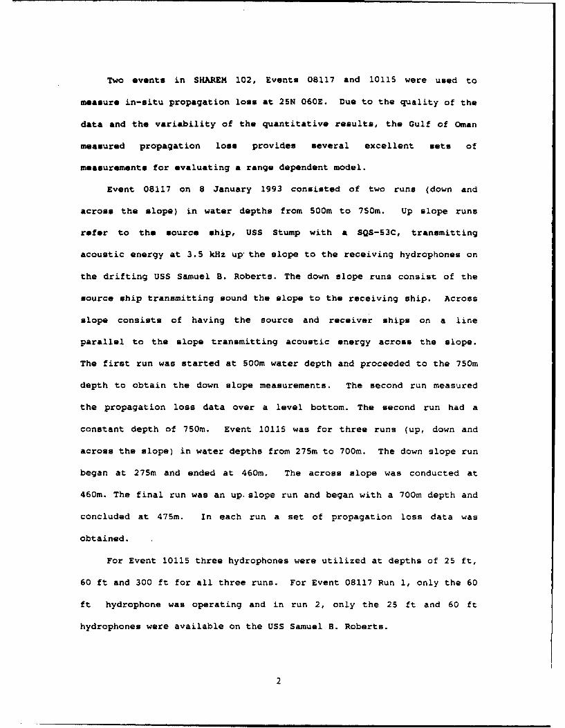
Two events in SHAREM 102, Events 08117 and 10115 were used to
measure in-situ propagation loss at 25N 060E. Due to the quality of the
data and the variability of the quantitative results, the Gulf of Oman
measured propagation loss provides several excellent gets of
measurements for evaluating a range dependent model.
Event 08117 on 8 January 1993 consisted of two runs (down and
across the slope) in water depths from 500m to 750m. Up slope runs
refer to the source ship, USS Stump with a SQS-53C, transmitting
acoustic energy at 3.5 kHz up the slope to the receiving hydrophones on
the drifting USS Samuel B. Roberts. The down slope runs consist of the
source ship transmitting sound the slope to the receiving ship. Across
slope consists of having the source and receiver ships on a line
parallel to the slope transmitting acoustic energy across the slope.
The first run was started at 500m water depth and proceeded to the 750m
depth to obtain the down slope measurements. The second run measured
the propagation loss data over a level bottom. The second run had a
constant depth of 750m. Event 10115 was for three runs (up, down and
across the slope) in water depths from 275m to 700m. The down slope run
began at 275m and ended at 460m. The across slope was conducted at
460m. The final run was an up. slope run and began with a 700m depth and
concluded at 475m. In each run a set of propagation loss data was
obtained.
For Event 10115 three hydrophones were utilized at depths of 25 ft,
60 ft and 300 ft for all three runs. For Event 08117 Run 1, only the 60
ft hydrophone was operating and in run 2, only the 25 ft and 60 ft
hydrophones were available on the USS Samuel B. Roberts.
2
A propagation loss range plot was generated at each hydrophone
depth for each run. A comparison between the propagation loss
generated by MAPS and measured data is the basic purpose of the thesis.
The impact of environmental data inputs such as bottom loss, bathymetry,
and XBT locations on the generation of propagation loss is investigated.
Finally the MAPS model/system is assessed as to its usefulness to an
Anti-Submarine Warfare Commander for shallow water tactical decisions.
3
II. DESCRIPTION OF MAPS
A. INTRODUCTION TO NAPS
The Multi-environment AIM Prediction System (MAPS) is a real time
range dependent expansion of- the Navy's standard RAYMODE propagation
loss model for active sonar. Range dependent RAYMODE is being developed
by Dr. Leibiger and MAPS was developed by Steve Dasinger of The Naval
Undersea Warfare Center, New London, Connecticut. MAPS was developed to
accurately predict propagation loss in highly variable environments for
use with the AN/SQS-26/53 sonar systems. It has the capability to
continually update the environmental data bases for potential
operational areas.
B. NAPS INPUT
MAPS begins with a query of own ship sonar parameters. This first
set of queries includes updating own ship's speed and sonar sector
center, own ship's heading and own ship's sonar characteristics.
Information about sonar parameters such as source level, signal
differential noise, signal differential reverberation, and own ship
noise default to sonar self-measurements in the ship-installed version,
but the user may alter these parameters if needed. Pulse length is
another query which adds important information to increase the accuracy
of the prediction. The last tactical information required is Target
Strength. Once own ship data, is updated, the user updates the
Environmental Input Data.
The Environmental Inputs Data is updated by entering a date/time
and Lat/Long which begins the setup for proper data file extraction of
4
the historical data bases. The Lat/Long entry can be used in one of two
ways. If the ship has XBT information from another ship along the track
of interest then the Lat/Long will be the entry for the location of the
obtained XBT information. Once all the XBT information from other
sources has been entered, then the final XBT information is entered at
own ship's position.
With the Lat/Long and date entry for own ship data, MAPS
determines whether there is data in the historical data base to
calculate propagation loss in the area of interest (AOI). The first
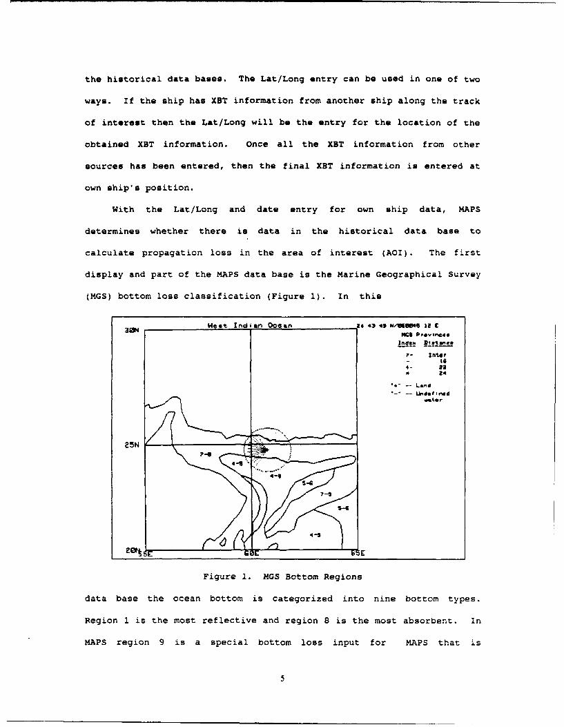
display and part of the MAPS data base is the Marine Geographical Survey
(MGS) bottom loss classification (Figure 1). In this
0Hot Indian Ocean 41 43 46 N/Wl0,61 i1 C"Cc Peviness
Inde. ,tawega
Po Inle
La4- 22
24
-- Land"-" -- Undefined
7-•
UA•
Figure 1. MGS Bottom Regions
data base the ocean bottom is categorized into nine bottom types.
Region 1 is the most reflective and region 8 is the most absorbent. In
MAPS region 9 is a special bottom loss input for MAPS that is
5
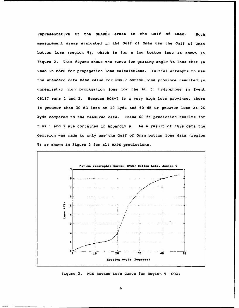
representative of the SHAREM areas in the Gulf of Oman. Both
measurement areas evaluated in the Gulf of Oman use the Gulf of Oman
bottom loss (region 9), which is for a low bottom loss as shown in
Figure 2. This figure shows the curve for grazing angle Vs loss that is
used in MAPS for propagation loss calculations. Initial attempts to use
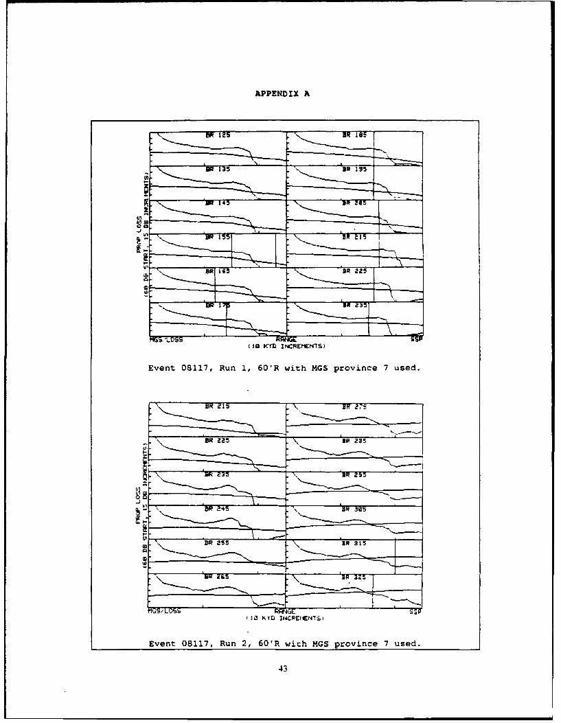
the standard data base value for MGS-7 bottom loss province resulted in
unrealistic high propagation loss for the 60 ft hydrophone in Event
08117 runs 1 and 2. Because MGS-7 is a very high loss province, there
is greater than 30 dB loss at 10 kyds and 60 dB or greater loss at 20
kyds compared to the measured data. These 60 ft prediction results for
runs 1 and 2 are contained in Appendix A. As a result of this data the
decision was made to only use'the Gulf of Oman bottom loss data (region
9) as shown in Figure 2 for all MAPS predictions.
"Nariln Geographic Survey (MGS) Dotto^ Loan, Region 99
7 . .. ..
4 - ... ............ ! . . .. tf3 - ... . .. =.. .. .... . .. .. ... .- , .
Z1 . ... .. ... .. .... ....
.... . . .... . ........ . . . . . . . . .; i . . . .:. . . . . . . . .
..
/ i/
8 is 28 38 49 so
Grazing Angle (Degrees)
Figure 2. MGS Bottom Loss Curve for Region 9 (GOO)
6
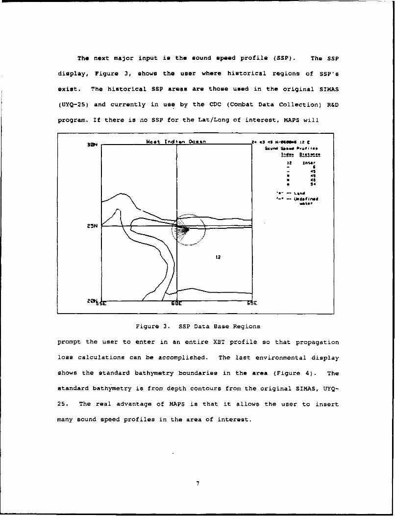
The next major input is the sound speed profile (SSP). The SSP
display, Figure 3, shows the user where historical regions of SSP's
exist. The historical SSP areas are those used in the original SIMAS
(UYQ-25) and currently in use by the CDC (Combat Data Collection) R&D
program. If there is no SSP for the Lat/Long of interest, MAPS will
30N woot Indian Ocean ,4 3 45 NWX4'I1e 12 Csoued Speed prat#s le,
IIde DIftl ¶. e
- I
- 45C 49e 462 54
'-" Undefined
Figure 3. SSP Data Base Regions
prompt the user to enter in an entire XBT profile so that propagation
loss calculations can be accomplished. The last environmental display
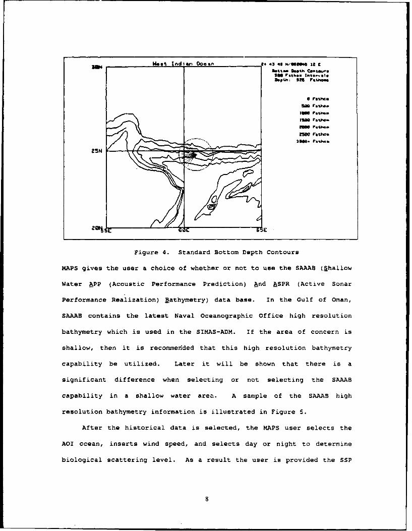
shows the standard bathymetry boundaries in the area (Figure 4). The
standard bathymetry is from depth contours from the original SIMAS, UYQ-
25. The real advantage of MAPS is that it allows the user to insert
many sound speed profiles in the area of interest.
7
Weot Indian Oeaon 14 43 43 NM/fU5, it 9
bott. north ce~a"Wro
north;iAn Fathom
a Trov e
F rB•i FDhomo
MAP rg•wdhalow Ftho•Im
Figure 4. Standard Bottom Depth Contours
MAPS gives the user a choice of whether or not to use the SAAAB (_Shallow
Water APP (Acoustic Performance Prediction) And ASPR (Active Sonar
Performance Realization) Bathymetry) data base. In the Gulf of Oman,
SAAAB contains the latest Naval Oceanographic Office high resolution
bathymetry which is used in the SIMAS-ADM. If the area of concern is
shallow, then it is recommerided that this high resolution bathymetry
capability be utilized. Later it will be shown that there is a
significant difference when selecting or not selecting the SAAAB
capability in a shallow water area. A sample of the SAAAB high
resolution bathymetry information is illustrated in Figure 5.
After the historical data is selected, the MAPS user selects the
AOI ocean, inserts wind speed, and selects day or night to determine
biological scattering level. As a result the user is provided the SSP
8
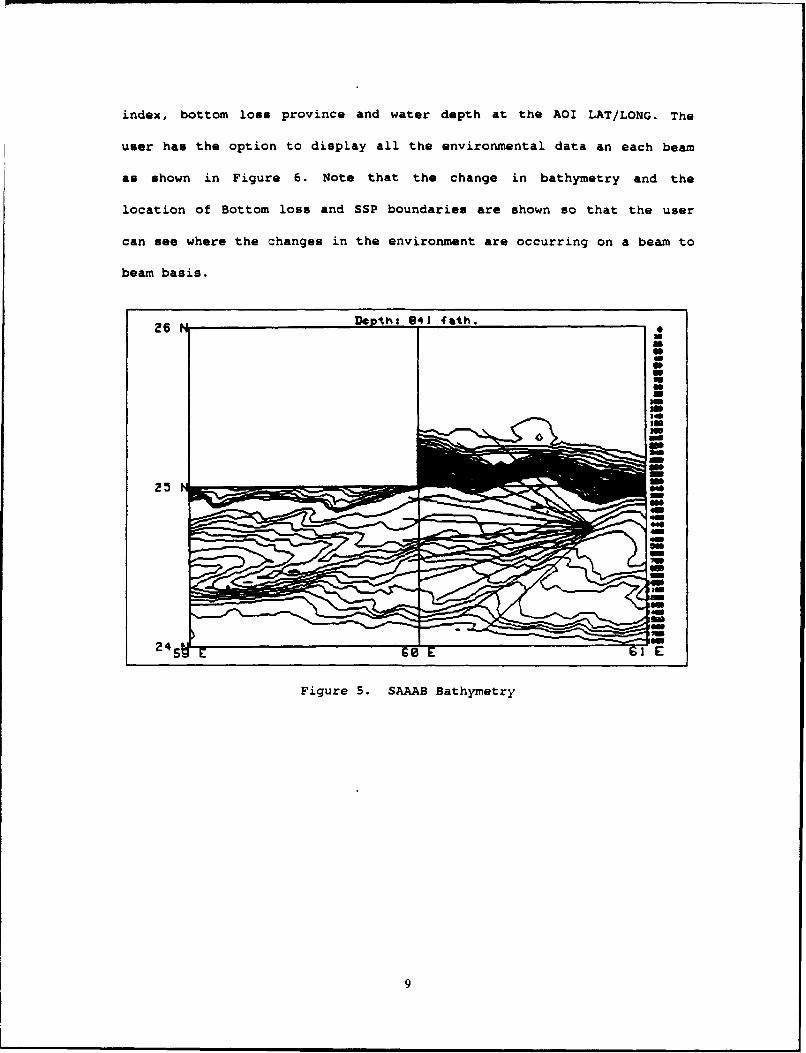
index, bottom loss province and water depth at the AOI LAT/LONG. The
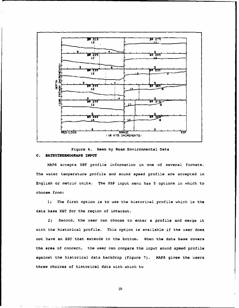
user has the option to display all the environmental data an each beam
am shown in Figure 6. Note that the change in bathymetry and the
location of Bottom loss and SSP boundaries are shown so that the user
can see where the changes in the environment are occurring on a beam to
beam basis.
26N Depth: 941 fath.
5 E I
Figure 5. SAAAB Bathymetry
9
ER 11 ei IR 275
12 ._.
9 2 4
1 26
(20 KYn INCRENENTS3
Figure 6. Beam by Beam Environmental Data
C. BATEYTHERMOGRAPH INPUT
MAPS accepts XBT profile information in one of several formats.
The water temperature profile and sound speed profile are accepted in
English or metric units. The SSP input menu has 5 options in which to
choose from:
1) The first option is to use the historical profile which is the
data base XBT for the region of interest.
2) Second, the user can choose to enter a profile and merge it
with the historical profile. This option is available if the user does
not have an XBT that extends to the bottom. When the data base covers
the area of concern, the user can compare the input sound speed profile
against the historical data backdrop (Figure 7). MAPS gives the users
three choices of historical data with which to
10
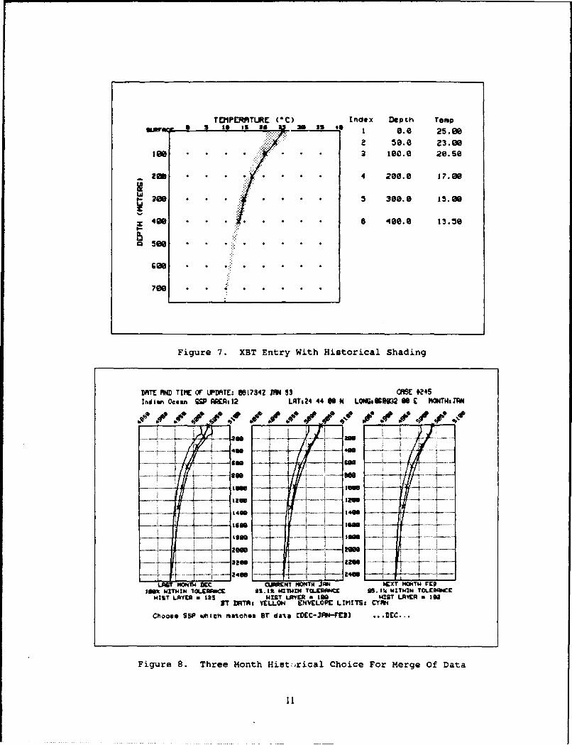
TC11PER"TURE (*C) Indeox Depth TemtpuWOKf a 5 is is as U 1mi 0.0 25.60
3 0.0 23.00lee a 100.0 29.50
2 m ** *4 200.0 17.00
**5 300.0 15.60
S490 6 '400.0 13.,5e
GeeS ..
SO'S .* . . . .
Figure 7. XBT Entry With Historical Shading
DATE FND TIME Of UPDATE; 00734Z PIN 93 GRSE 045Indian Oesan SGP ARCtil2 LRT&24 44 0 N LOW~ASflB 88 E MWNTPAYR
APa I ce 0 APO
.. ..... ....... ...* .. --- ---
......~~~~~~~ ~ ~ ~ ....... . ... 4 ..... . .. ...
La w ..... ..... .... -- - ---- i m ......
lo w ....... ... .....-
...... ..... 1206 - ....
LAST MNTH4 DEC UCIMPEN I~MOT JANJ IXT MONTH FEB1ftX WITHIN 1OLERANCE SS.t bGTWIMh Ta..CRNCI 2S.1U~ WITHIN TOLERANCE
MIST LAYER a 125 MIST LAYER MISO14ST LR'vKP a 19IT DAThs YELLON k.NVLOPPC LIMITi: CYAN
Cooese SSP b~slch artehes ST da-te CDEC 3J4-VCEB .. .DEC..
Fi.gure 8. Three Month Hist jri.cal Choi.ce For Merge Of Data
merge the in-situ XBT. The center profile is the month that had been
entered previously and the two other profiles are the months previous to
and following the month inputted (Figure 8). This allows the user the
option compare the XBT with the historical data base monthly data on
either side of the month of interest.
3) The third option is to enter an entire profile to the bottom
depth. This option gives the user the capability of using the in situ
XBT data without merging to the historical SSP. This option gives the
user the capability of entering up to 25 SSP's at different locations
that can be used in the range dependent propagation loss calculations.
4) The fourth option is for the user to select one of the last ten
XBT's on file.
5) The final option is to use the last SSP that was entered. This
is a useful option and reduces data input time.
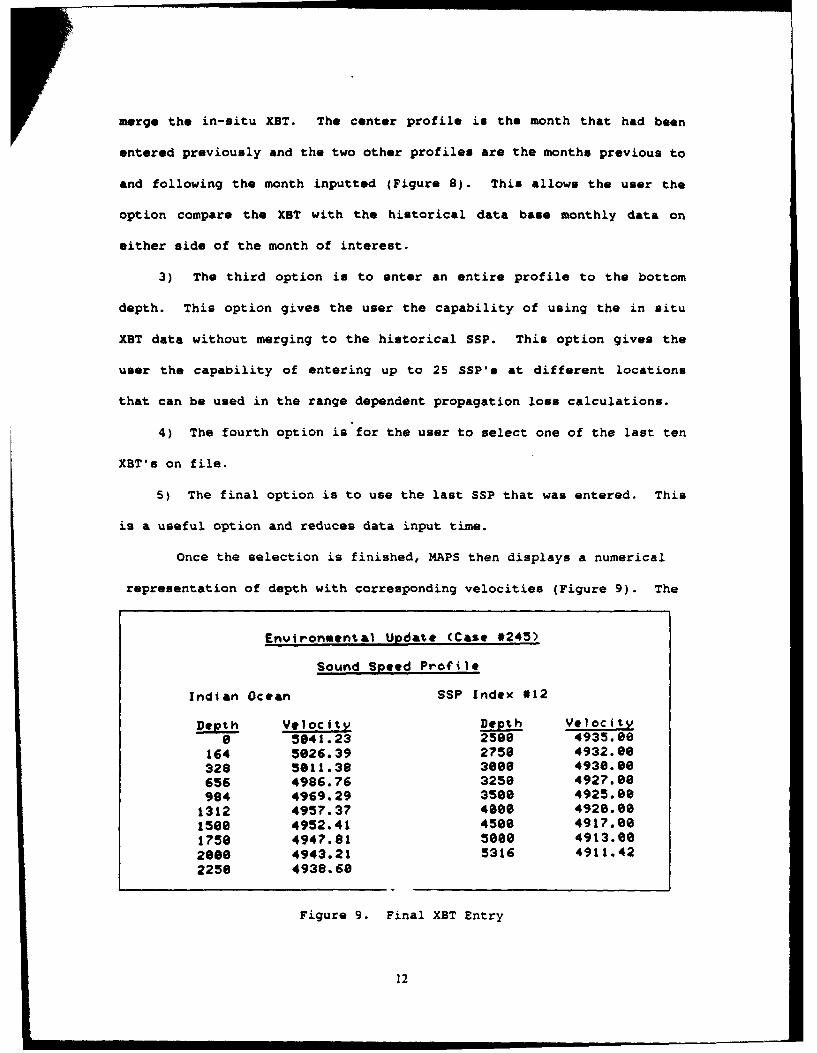
Once the selection is finished, MAPS then displays a numerical
representation of depth with corresponding velocities (Figure 9). The
Environmental Update (Case *245)
Sound Speed Profile
Indian Ocean SSP Index #12
Depth Velocitg Depth Velocity0 5041.23 2500 4935.00
164 5026.39 2758 4932.00328 5011.38 3000 4930.00656 4986.76 3250 4927.00984 4969.29 3500 4925.00
1312 4957.37 4000 4920.8015ee 4952.41 4500 4917.801750 4947.81 5000 4913.002000 4943.21 5316 4911.422250 4938.60
Figure 9. Final XBT Entry
12
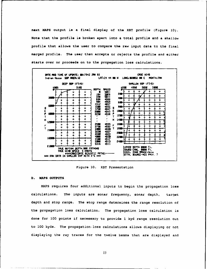
next MAPS output is a final display of the XBT profile (Figure 10).
Note that the profile is broken apart into a total profile and a shallow
profile that allows the user to compare the raw input data to the final
merged profile. The user then accepts or rejects the profile and either
starts over or proceeds on to the propagation loss calculations.
DAEIT D TIME O UPDATE; 01S74Z JM 33 CRS 445Indian, Ocuan SGP RIl2 LATs24 44 W N LONGgsU2 U09 E NOTIIIaJAN
DEEPMP (Mo4 I 9RL.LON S5P (F'T/)M435 5165 WE 498"0 53 58W
+' 6 5341 + + ++. + 154 582 2W-.-329 5B)I
+ + + 956 436 + 4 + ++ 33 94 4113 600-.......4- 4
-- 4- 1312 4057 4 + + +15 4 43521 18 .. + $ $+. + + 175 4947 4 + +
E + + t+ 29m 4343 E 100-- 4-P 4- 4- - 2low 432 P+
T + + T T1--+ 4 + + 1140-
1235 -4- -4--*-+ 4+ + +, 4t.,9
T. 30M. 5 4 5 3 5 r 7 -16-WT sm.-..~. ---- ~3m3 43 -1+ -------
4+ + + M.4. + + 49235 4---4- .-4.
+Sl 4912 2
4+ + + 5318 4911 _
2135l + t LAYER DEPTH OW Ft.TMUE BOTTOM DEPTH ME F7•M:I6gNi o1a. e Ft..TRUE WIND SPED S KNOTS I CNV*. ZONE R•m t.E:Nn
tii•iT tt •NDIDATE RCOUSTIC PRTHS ----- .. . 1TTh. ZOL CE-IG P*s V.PAW DATA IN SHRL.LO SVP HW11 X'S ;
E P
Figure 10. XBT Presentation
D. MAPS OUTPUTS
MAPS requires four additional inputs to begin the propagation loss
calculations. The inputs are sonar frequency, sonar depth, target
depth and stop range. The stop range determines the range resolution of
the propagation loss calculation. The propagation loss calculation is
done for 100 points if necessary to provide 1 kyd range resolution out
to 100 kyds. The propagation.loss calculations allows displaying or not
displaying the ray traces for the twelve beams that are displayed and
13
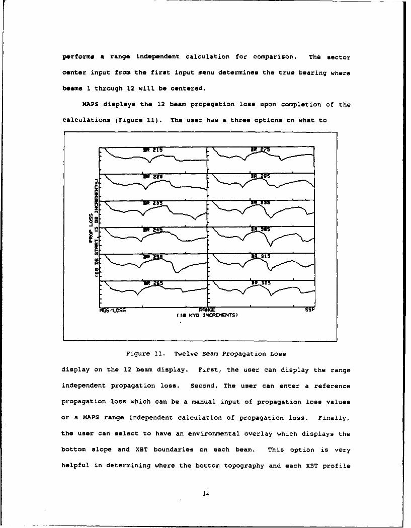
performs a range independent calculation for comparison. The sector
center input from the first input menu determines the true bearing where
beams 1 through 12 will be centered.
MAPS displays the 12 beam propagation loss upon completion of the
calculations (Figure 11). The user has a three options on what to
GS/tos$ 55F(10 K<YD INCRqEMENTS)
Figure 11. Twelve Beam Propagation Loss
display on the 12 beam display. First, the user can display the range
independent propagation loss. Second, The user can enter a reference
propagation loss which can be a manual input of propagation loss values
or a MAPS range independent calculation of propagation loss. Finally,
the user can select to have an environmental overlay which displays the
bottom slope and XBT boundaries on each beam. This option is very
helpful in determining where the bottom topography and each XBT profile
14
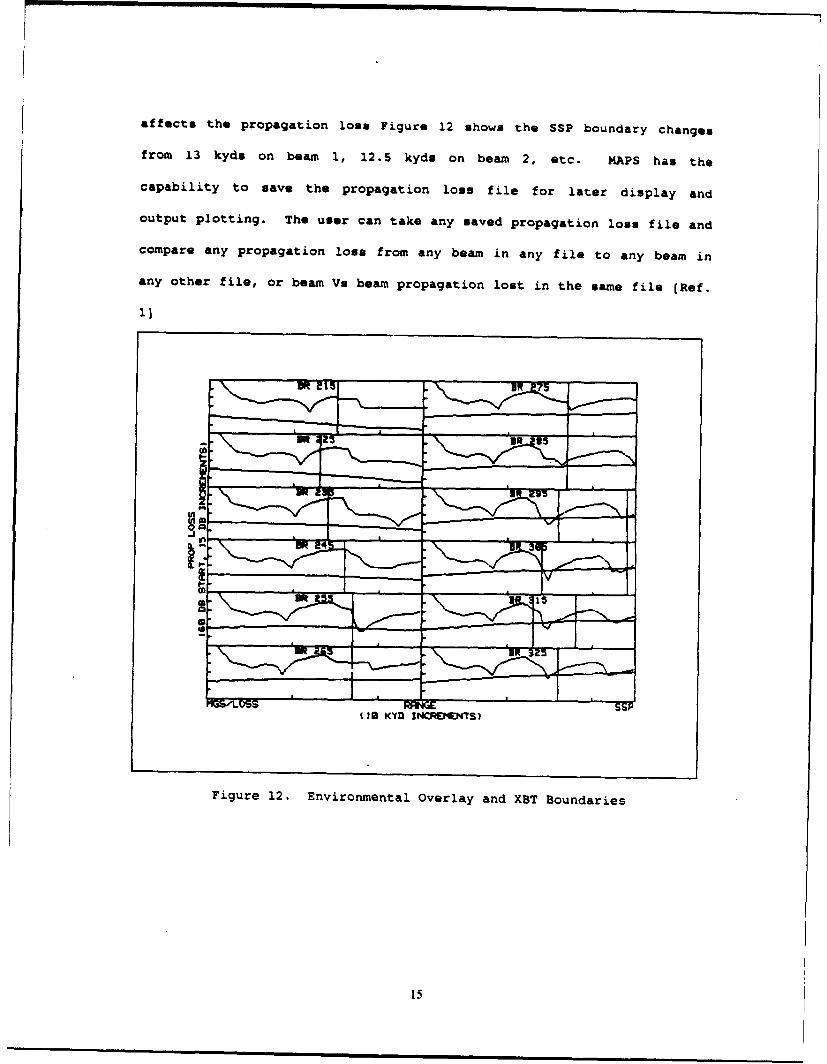
affects the propagation loss Figure 12 shows the SSP boundary changes
from 13 kyds on beam 1, 12.5 kyd. on beam 2, etc. MAPS has the
capability to save the propagation loss file for later display and
output plotting. The user can take any saved propagation loss file and
compare any propagation loss from any beam in any file to any beam in
any other file, or beam Vs beam propagation lost in the same file (Ref.
1]
DW-
Figure 12. Environmental Overlay and XBT Boundaries
15
Sm • • • • mI m m SL|
III. HIGH RESOLUTION 3ATHYMETRY
The SAAAB high resoluti6n bathymetry data base has been upgraded
for the Gulf of Oman areas of interest by use of special Naval
Oceanographic Office bathymetry data. This upgraded bathymetry has
significantly enhanced the use of the bottom topography. The bathymetry
information has 10 fathom contours up to 100 fathoms, 20 fathom contours
from 100 to 500 fathoms and, thereafter, 100 fathom contours. To
evaluate the difference between the SAAAB data base and standard
bathymetry data base, a trial case was run to illustrate the importance
of bathymetry accuracy in calculations of propagation loss.
In Chapter II in Figures 4 and 5 the large difference in bottom
contour definition between the SAAAB and standard data bases was
identified. In this trial case a 60 ft receiver depth and 25 ft source
depth was used. The first difference in the two data bases is the
bottom depth calculation at own ship's position at 24-43N 060-46E. In
the standard data base the water depth was 920 fathoms and the SAAAB
data base produced a water depth of 841 fathoms, about a 10% difference.
The bearing of interest for this trial case was 275 degrees true.
Utilizing the capability of MAPS to overlay the bottom contours on the
beam by beam propagation loss display and isolating the bearing of
interest through a software modification that also removed the
propagation loss curve, Figures 13 and 14, were generated. It is
evident that the SAAAB data base provides a more detailed bathymetry
16
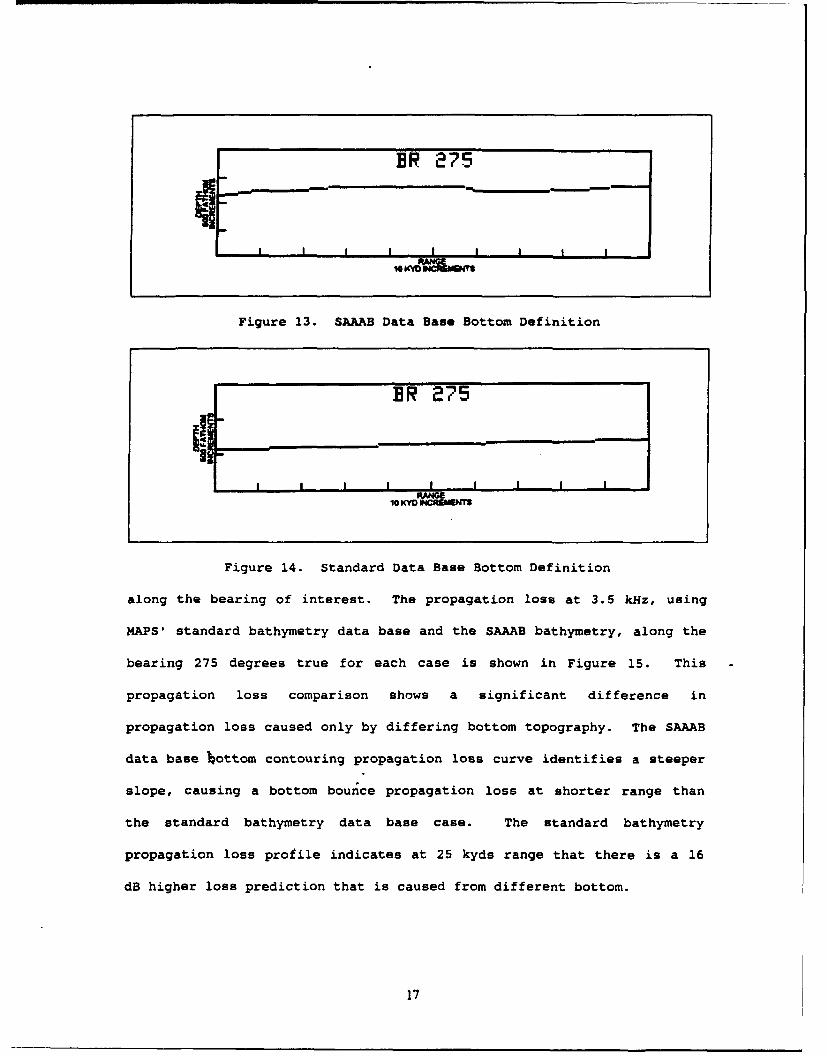
ER 275
Figure 13. SAAAB Data Base Bottom Definition
ER 275
I I I I I I I
Figure 14. Standard Data Base Bottom Definition
along the bearing of interest. The propagation loss at 3.5 kHz, using
MAPS' standard bathymetry data base and the SAAAB bathymetry, along the
bearing 275 degrees true for each case is shown in Figure 15. This
propagation loss comparison shows a significant difference in
propagation loss caused only by differing bottom topography. The SAAAB
data base Iottom contouring propagation loss curve identifies a steeper
slope, causing a bottom bounce propagation loss at shorter range than
the standard bathymetry data base case. The standard bathymetry
propagation loss profile indicates at 25 kyds range that there is a 16
dB higher loss prediction that is caused from different bottom.
17
At 18 kyds there is a 21 dB lower lose than the standard data base.
These are significant changes in propagation loss that have strong
tactical implications in sonar system performance assessment. This
trial case shows a strong argument for a high resolution bathymetry data
base to be utilized to ensure the propagation loss calculations are as
accurate as possible. What is needed is to compare the accuracy of the
propagation loss predictions with actual measured propagation loss. For
the SHAREM 102 propagation loss measurements, the SAAAB bathymetry was
used in MAPS for development of the propagation loss predictions to
compare with the measured data.
18
SAAAB7ml + +
Oe + +,
lm + STANDARD
l ze+ +
S128 + +
136 + +
146 + +
1569I * I[ , • ,
15LB 20RRNGE (KYDS)
Figure 15. SAAAB Vs Standard Bathymetry Propagation Loss
19
IV. EVENT 08117
A. EVENT GEOMETRY AND PROCEDURES
The SHAREM 201 test plan called for environmental tests to measure
propagation loss. Each event, 08117 and 10115, utilized two ships to
conduct the tests with another ship collecting XBT data. The geometry
for the two ship transmission loss experiments is shown in Figure 16.
DD DD
COMEX 10 KNOTS FINEX-- "-FFG
1.5 KYDT IT 5 KNOTS *(DiW).5T-AGS T -AGSCOMEX FINEX
k- 10 KYD-• I- 5 KYD
__ _ - 25 KYD -I
Figure 16. 3 Ship Geometry
The FFG was drifting in the water. The DD began each test at
approximately 25 kyd away from the FFG and traveled 20 kyd toward the
FFG at a speed of 10 knots. The T-AGS (USNS Silas Bent) began
approximately 5 kyd from the FFG (Ref. 2:p5.]. The ship tracks for runs
1 and 2 for the DD and FFG are shown in Figure 17. The source frequency
from the DD's AN/SQS-53 for all tests were 3.5 kHz.
Measurements of XBTs that were taken during the entire SHAREM
exercise were analyzed by Naval Undersea Warfare Center Detachment New
20
London, CT. It was determined that there were 7 homogeneous regions of
sound speed profiles as shown in Figure 18 (Ref. 3]. Figure 15 shows
that Event 08117, runs 1 and 2, were conducted in an area of profile A.
Of the 7 profiles determined to exist, only profiles A, C and E were
profile areas that affected SHAREM propagation loss measurements. Any
XBTs that ere taken during the event and were in the area of the ship
AM:o6 EVENT 00117I•a I0:% 0101300 - 01061800ZI gfl U 142TIC INETAVW_..: IS. MIN
025 60o.k COMM R1UM1 02E 00 ON1526
FF6 Al
1627
______ 00
S.- ENT 081 025ZJAN931 091400
oa 150
1901FIXZX RUN 2 1734
cOx RUN 2
02 ?.O 024135ON
060-10. O -,SO. 0C
Figure 17. Event 08117 , Run 1 and 2 ship Tracks
tracks were entered into MAPS and are depicted on the Ship Tracks,
Figure 15. For the own ship XBT entry, the corresponding profile XBT
21
that is indicated on each ship track figure was used for the entry into
MAPS. All profile XBTs and in-situ XBTs that were utilized to conduct
MAPS runs are contained in Appendix B.
_....._ _064- - --
57• 58" • 0 a
Figure 18. Chart of Homogeneous Areas in Gulf of Oman
B. EVENT 08117 RESULTS
1. Run 1
For Event 08117, Run 1, only the 60 ft hydrophone was operating
due to mechanical problems with the 25 and 300 ft hydrophones. Run 1 is
a down slope run with the DD at a starting depth of 500 meters and
222
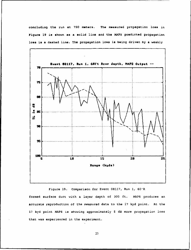
concluding the run at 750 meters. The measured propagation loss in
Figure 19 is shown as a solid line and the MAPS predicted propagation
loss is a dashed line. The propagation loss is being driven by a weakly
Zvent 88117, Run 1. 6Sft Rcvr depth, MAPS Output --
75
.. ....... ............... (................. .........................• .. ,...... .. .... ........ •....... ....... ...... .... . . . . . . . . . . . . . . . . . . . . . . . .
9 ..................................................... ...... . .. ..... .... . ....
................
9 ................. °........................................... . . . . . . . . .. ..... ........ r
5 is 1 28 25
Range (k~ds)
Figure 19. Comparison for Event 08117, Run 1, 60IR
formed surface duct with a layer depth of 300 ft. MAPS produces an
accurate reproduction of the measured data to the 17 kyd point. At the
17 kyd point MAPS is showing approximately 5 dB more propagation loss
that was experienced in the experiment.
23
2. Run 2
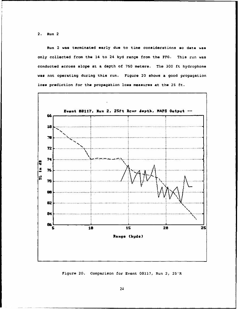
Run 2 was terminated early due to time considerations so data was
only collected from the 14 to 24 kyd range from the FFG. This run was
conducted across slope at a depth of 750 meters. The 300 ft hydrophone
was not operating during this run. Figure 20 shows a good propagation
loss prediction for the propagation loss measures at the 25 ft.
Event 88117, Run 2, 25tt Acur depth. MAPS Output --
•,o o .... .. ... . 0 ~ o. ol.......................... ........................... •.........................
7 . .................. \0 . . ,. ................... ,........ ......................... .........................
74 .......... ... . ..... , .....
4- 7 ......................... .• ..... ... .... •.-.... .... .... .. .... .... ... ....... ...........................
7 . ......................... .................... ....... ..........
Be . ........................ .......................... ..................... ... ......
2 .................................................................................... ........
8 4 .............. .... .. ... .......................... .......................... ................. ........
96.5 18 15 28 25
Range (k~ds)
Figure 20. Comparison for Event 08117, Run 2, 25'R
24
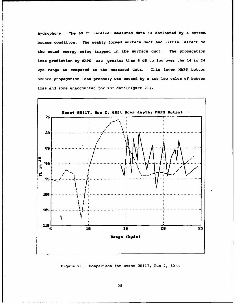
hydrophone. The 60 ft receiver measured data is dominated by a bottom
bounce condition. The weakly formed surface duct had little effect on
the sound energy being trapped in the surface duct. The propagation
loss prediction by MAPS was greater than 5 dB to low over the 14 to 24
kyd range as compared to the measured data. This lower MAPS bottom
bounce propagation loss probably was caused by a too low value of bottom
loss and some unaccounted for XBT data(Figure 21).
Event 98117. Run 2. 68ft Rcvr depth. NAPS Output --
75
//
/ \ :B e .......................... ......... It .............. •• ........ .. ............. ......................... .i//
S" 0 .. . .. . . . . .. . . .• ....................... . . . . .. . . ... .
r 90 ' ' .... . .. ........ •............ .. Al...... . . . . . . . . .I:
lee6 ......... \........ Al . .............. ..;............ ... . ......... ..................
U I /:-I/:
is @ .. ..... ... . .. ....... ..... ......................... %..........................
6 ................... . .
5 ie is 20 25
Range (kqd8)
Figure 21. Compari~on for Event 08117, Run 2, 60IR
25
V. EVENT 10115
A. RUN 1
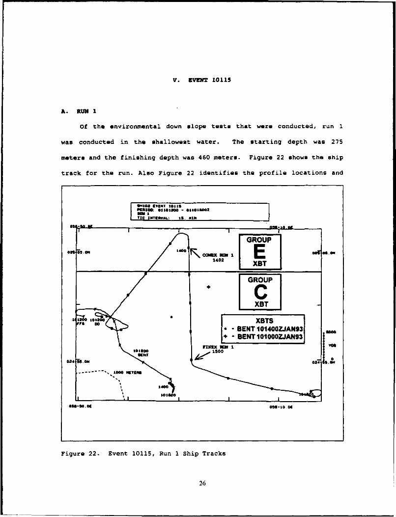
Of the environmental down slope tests that were conducted, run 1
was conducted in the shallowest water. The starting depth was 275
meters and the finishing depth was 460 meters. Figure 22 shows the ship
track for the run. Also Figure 22 identifies the profile locations and
M11*.IT 10*13I ""°s souo -*a1e0TZC INTERVAL: is. "I"
GROUP0 OSIM . E Otl "."
1402 XBTP
GROUP
IC
Aria 101200 XBTS
S - BENT 101400ZJAN93 am024 551 *'BENT 101OOOZJAN93 OI
-'M110 100500E0 2 " b . . . . ," 0 2 1 5 .4 1
M410
Ooa-iO. 0 O50-O. .0
Figure 22. Event 10115, Run 1 Ship Tracks
26
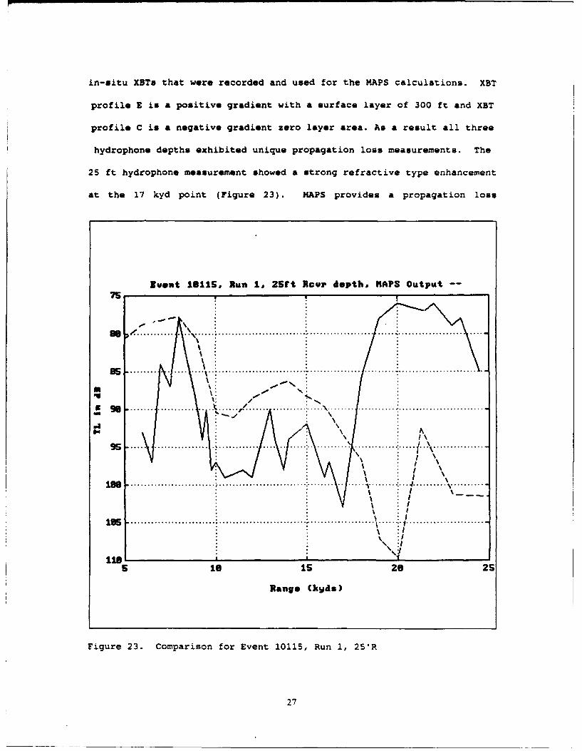
in-situ XBTs that were recorded and used for the MAPS calculations. XBT
profile E is a positive gradient with a surface layer of 300 ft and XBT
profile C is a negative gradient zero layer area. As a result all three
hydrophone depths exhibited unique propagation loss measurements. The
25 ft hydrophone measurement showed a strong refractive type enhancement
at the 17 kyd point (Figure 23). MAPS provides a propagation loss
Zvent 1B115, Run 1, 2Sft Rcut depth, MAPS Output --75
E . ....... . .. . . ..... ..... ... . ...... .. .. ..... ..... ..
me. ..........
g. .. . ....... . . . . .
.. ... . ...... ............. . . .
9 ... . .......... . . . .... ..0 . °o . . . . . .. ............. . ..........
: : lI \ _S.. .................................................................. -
1BS .........9. o..... ..... .. .... ................. ....................... ...... .
lie,g\ :1\ Ji
118 1
5 is 15 20 25
Range (Chds)
Figure 23. Comparison for Event 10115, Run 1, 25'R
27
prediction that is approximately 5 dB to 10 dB lower than the measured
data until the 17 kyd point. It is at this point that MAPS does not
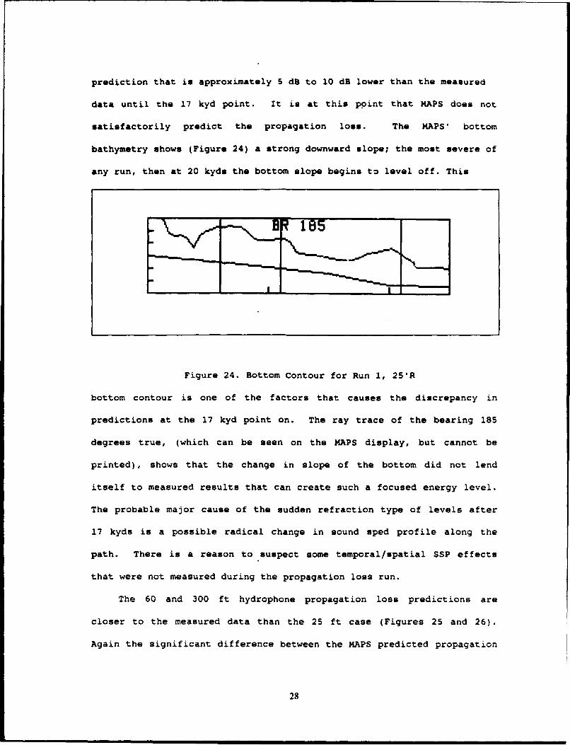
satisfactorily predict the propagation loss. The MAPS' bottom
bathymetry shows (Figure 24) a strong downward slope; the most severe of
any run, then at 20 kyds the bottom slope begins to level off. This
Figure 24. Bottom Contour for Run 1, 25*R
bottom contour is one of the factors that causes the discrepancy in
predictions at the 17 kyd point on. The ray trace of the bearing 185
degrees true, (which can be seen on the MAPS display, but cannot be
printed), shows that the change in slope of the bottom did not lend
itself to measured results that can create such a focused energy level.
The probable major cause of the sudden refraction type of levels after
17 kyds is a possible radical change in sound sped profile along the
path. There is a reason to suspect some temporal/spatial SSP effects
that were not measured during the propagation loss run.
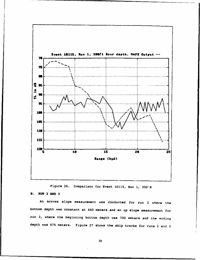
The 60 and 300 ft hydrophone propagation loss predictions are
closer to the measured data than the 25 ft case (Figures 25 and 26).
Again the significant difference between the MAPS predicted propagation
28
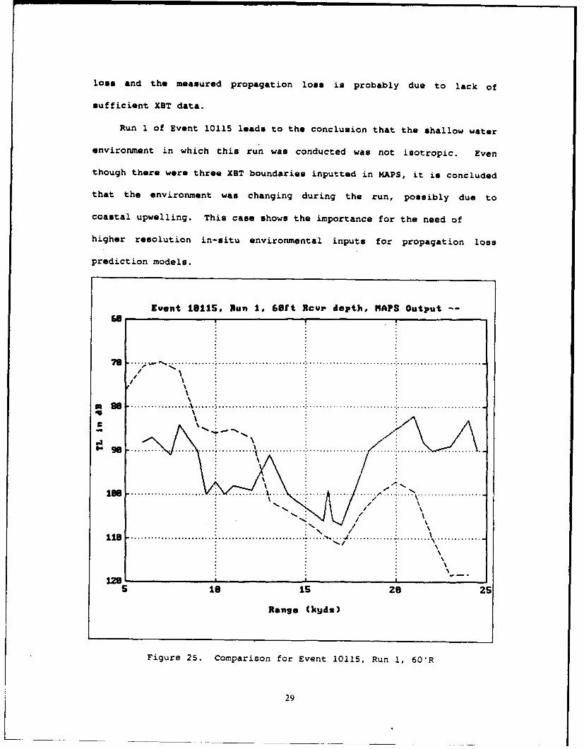
loss and the measured propagation loss is probably due to lack of
sufficient XBT data.
Run 1 of Event 10115 leads to the conclusion that the shallow water
environment in which this run was conducted was not isotropic. Even
though there were three XBT boundaries inputted in MAPS, it is concluded
that the environment was changing during the run, possibly due to
coastal upwelling. This case shows the importance for the need of
higher resolution in-situ environmental inputs for propagation loss
prediction models.
Event 19115, Run 1, 6Sft Rovi depth, MAPS Output --
/ N
//
I\\
U\. .. . . . . . . .... . ... . $o ... .. o. . . . . . . . ... . . . . . . .. . .. ... . ,.... .. . . . . . .. . . .. .. . .. .. . . .. . . .. . . . . .. .. . . . .. .. . .. . . .
* /\
go1 .......... ....... ..... ........ ......... %........................ .... .......
p \
128,s 18 is 28 25
Range Chqds)
Figure 25. Comparison for Event 10115, Run 1, 60'R
29
Event 16115, Run 1. 30Oft Rcvv depth. MAPS Output --
76
g o . . . . . ............ Io,. ° ........................ o°..... .......................... .........................
.. . . . . ....... . ... .. .. .................
e ....... ...... ... .. ... . ....... :. . . ' 'l """ . . . . .:. . . . . ..\ . .
1 1 ......................... •.......................... %. .......................... :................ il........
- a/ %%
i .................................................... :.......................... -.................... . .
s is is 26 25
Raenge (hyd)
Figure 26. Comparison for Event 10115, Run 1, 300'R
S. RUN 2 AND 3
An across slope measurement was conducted for run 2 where the
bottom depth was constant at 460 meters and an up slope measurement for
run 3, where the beginning bottom depth was 700 meters and the ending
depth was 475 meters. Figure 27 shows the ship tracks for runs 2 and 3
30
IU!
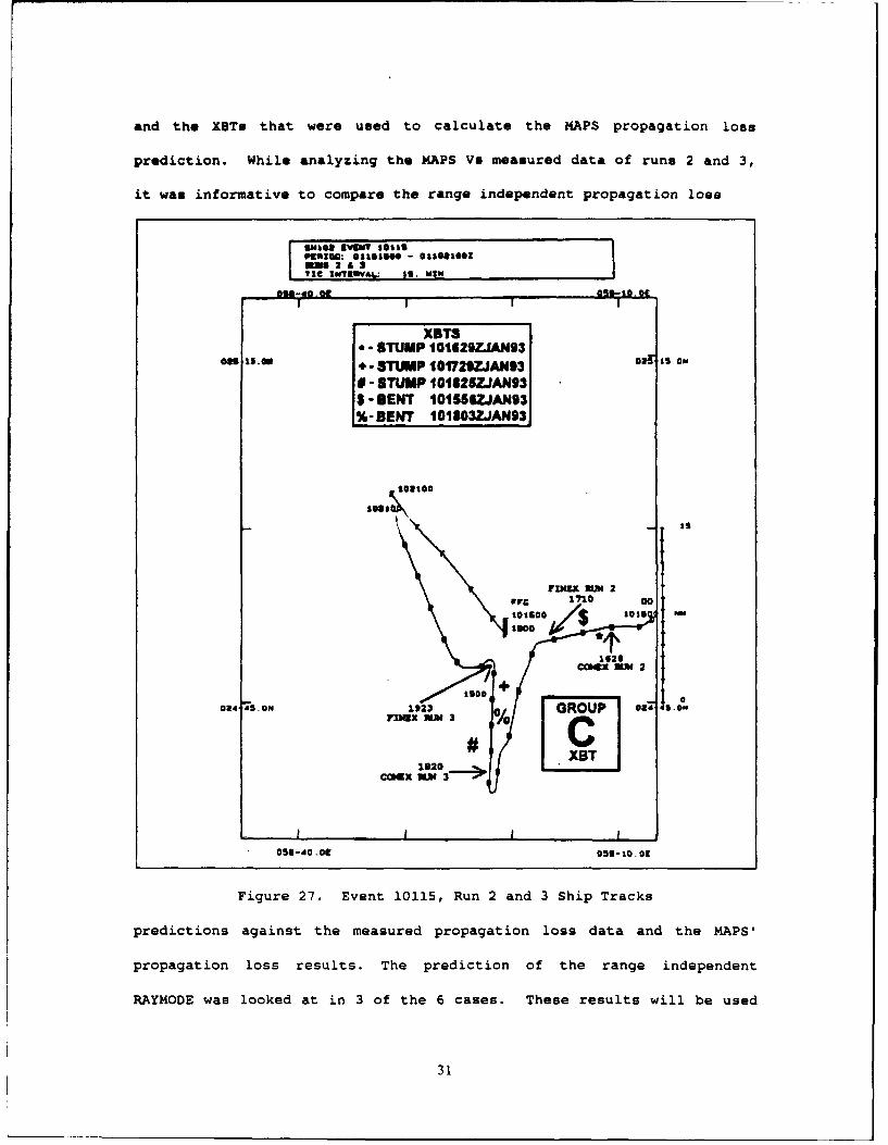
and the XBTs that were used to calculate the MAPS propagation loss
prediction. While analyzing the MAPS Vs measured data of runs 2 and 3,
it was informative to compare the range independent propagation loss
060110: 0&less6" - ol0 0oozmINDI 2 as2TIC "S•eV . sI. -IN ,
owido, t csj010 . DI; I I I
XBTSSTUMP 101629ZJAN93
05. 4sin *- STUMP 101729ZJAN93 0 o,,
" - STUMP 10182SZJAN93$ - SENT 10155T.JAN93%-BENT 101803ZJAN93
o10300
Solis
YIN= 21710 00
101014 los
1620
COM@, IM 2
lo00 +Olad ;SON 1923 0 GROUP o O .oN
C0X 1"320>
I I I
O51-dO l 0 059-10.0
Figure 27. Event 10115, Run 2 and 3 Ship Tracks
predictions against the measured propagation loss data and the MAPS'
propagation loss results. The prediction of the range independent
RAYMODE was looked at in 3 of the 6 cases. These results will be used
31
to illustrate the importance of using a range dependent model such as
MAPS in a shallow water environment Vs a range independent model. For
the 3 cases that address the range dependent case Vs the range
independent case, the range independent case was added to the comparison
plots. The other 9 range independent plots are found in Appendix B for
back ground reference.
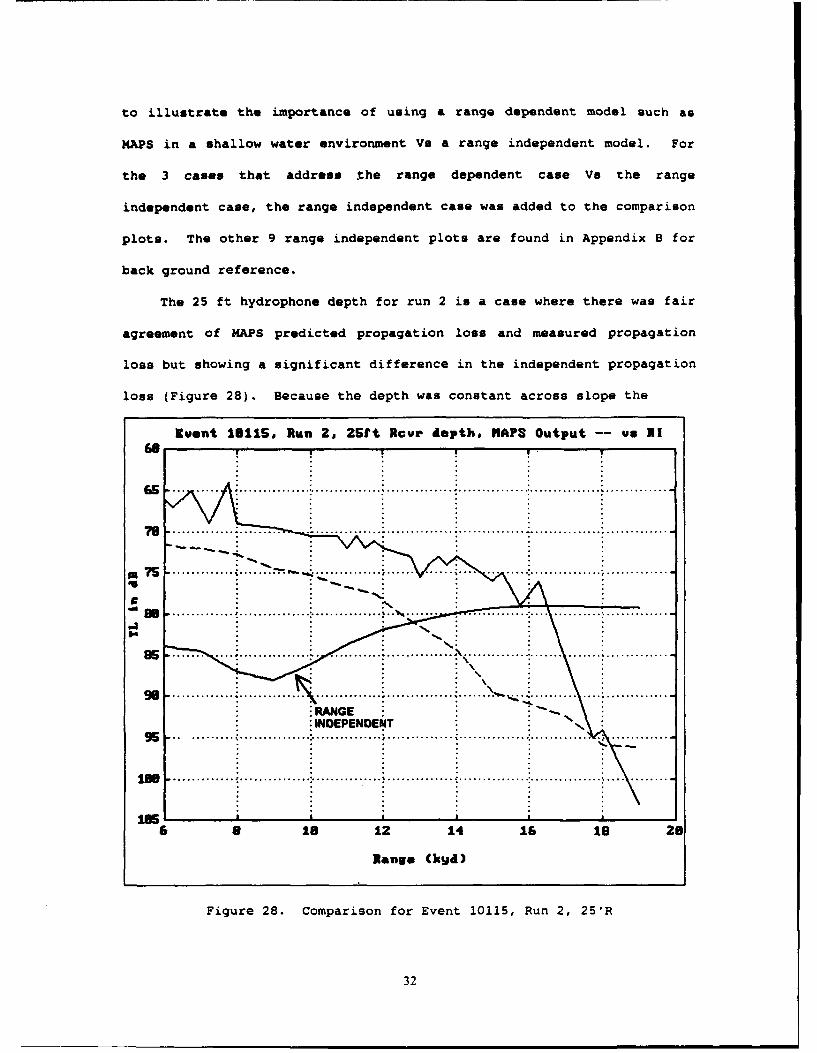
The 25 ft hydrophone depth for run 2 is a case where there was fair
agreement of MAPS predicted propagation loss and measured propagation
loss but showing a significant difference in the independent propagation
loss (Figure 28). Because the depth was constant across slope the
Event 19115. Run 2, 25ft Rcvr depth. HAPS Output -- us R!
6 6 18 1 14 16.2
.. . ........... • ....... ........... ...... ... ..... : ............... :* I *I - - .............
75 ....... .........:........... ... ... .. .... ....... ................................. .... ... .. ... ..........• .... ......... ...............
9 .... ... .. .. ......... . ........ ........ ....... .............
Fu 2 o n f Ev e 1 , R
32
difference must be because of the different XBT regions across the
propagation path. Profile C was used as the XBT entry at own ship
position, which showed a negative gradient. The lack of the surface
duct is what causes the difference in the MAPS' prediction and the range
independent prediction compared to measured data. The measured data was
in a strong surface duct that accounts for the low propagation loss
through the 16 kyd point. The MAPS range dependent model was not able
to correctly predict the propagation loss due to the multiple XBT types
across the propagation path because the baseline XBT "C" negative
profile was used at own ship. Because of C's negative profile the range
independent propagation shows high surface duct and bottom bounce
propagation.
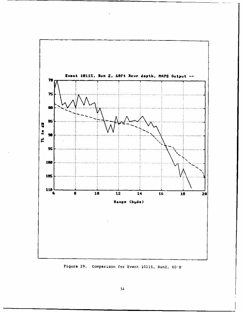
The 60 ft hydrophone measured data and the MAPS propagation loss
prediction are in close agreement across the testing range until 17 kyds
where a strong downward refraction condition occurred (Figure 29). The
300 ft hydrophone measurement was accurately predicted by MAPS (Figure
30).
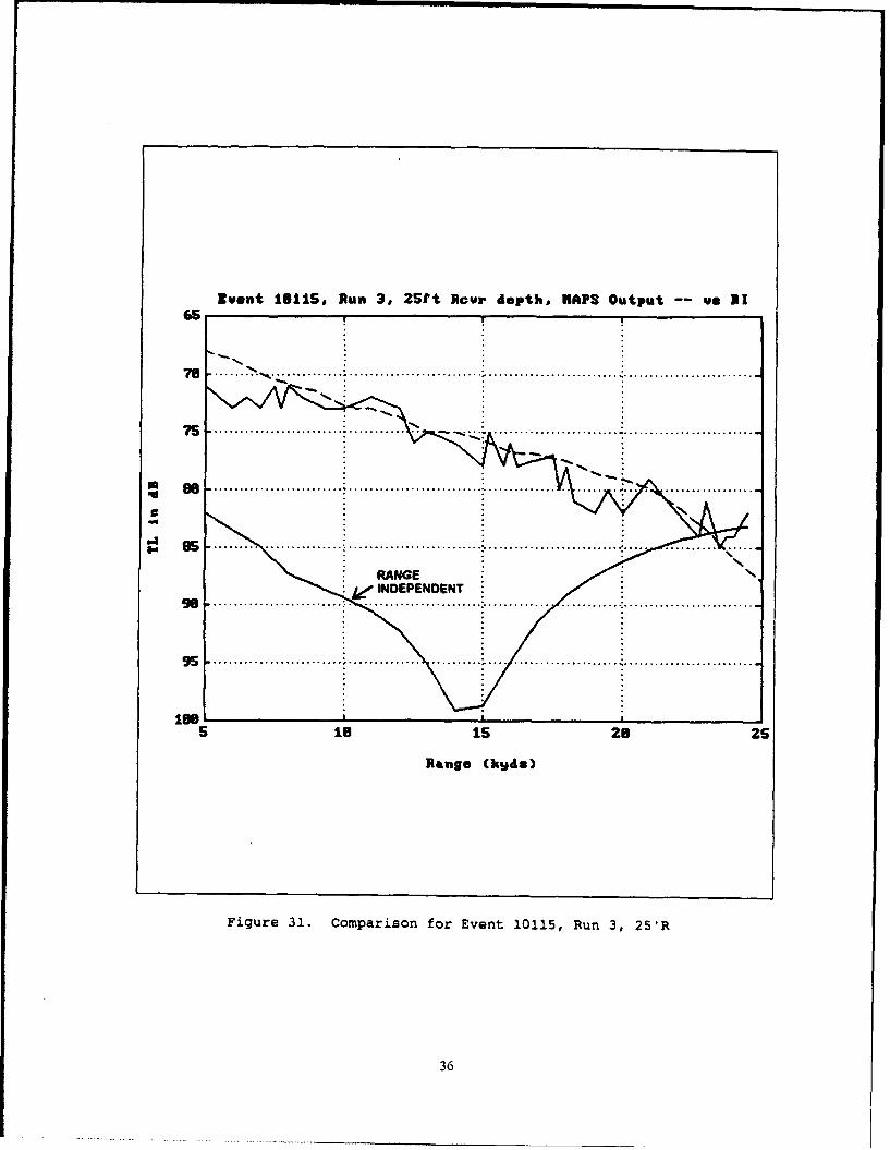
For run 3 the 25 ft hydrophone case is a strong example of where
the range dependency and the changing environment must be taken into
consideration to accurately predict propagation loss in a shallow water
environment. MAPS accurately predicts the propagation loss (Figure 31),
however the range independent prediction was 20 dB to 40 dB to high in
loss as compared to measured data and indicates a bottom bounce
propagation situation at 15 kyd.
33
Event 18115, ]Run 2, 68ft Xcua depth, MAPS Output --
S . . . ......... .i . . ........ . ............... : . ... ,. . . .............. . ............... •.............
..... ... . . ... . .. .. .. . ... .. ..... * . ............ " ..... ... ....... :............... i..............
"9 . . . . . . .z. . . . . .. . . . . . . . . . . . . ....... : .. . . .. . . . . . . . . . . . .
S S0 . ............. : . ................. - .... .- ... .. .... .. -.... ............... i .............
SS3.i . "
1 8 5 .......................... .. ............. .. . .. . ............ ........ .... ........ .. .. ......
11B8 LJ6 8 18 12 14 16 19 28
Range (kyds)
Figure 29. Comparison for Event 10115, Run2, 60'R
34
Event 18115. Run 2, 308ft Rcur depth, MAPS Output --
as
a . . . . . . . . .. . . . . . . . . . . . . . . . . . . . . . . . . . . . . . . . . . . . . . . . . . . . . . . . . . . . . . . . . . . . . . . . . . . . . . . . . . . . . . .
9 0• .. . . . . . . . . . . . . . . . . . . .. . .... . . . . . . . . . . . . . . . . . . . . . . . .
95....... .................................................
l . •. .. . .
es ........................ .....
i e ..-.... ... -.. ......... ...... ...... ........... .............. ........ .... ............. ... ............
6 s is 12 14 16 is 218
Range (kgd$)
Figure 30. Comparison for Event 10115, Run 2, 300IR
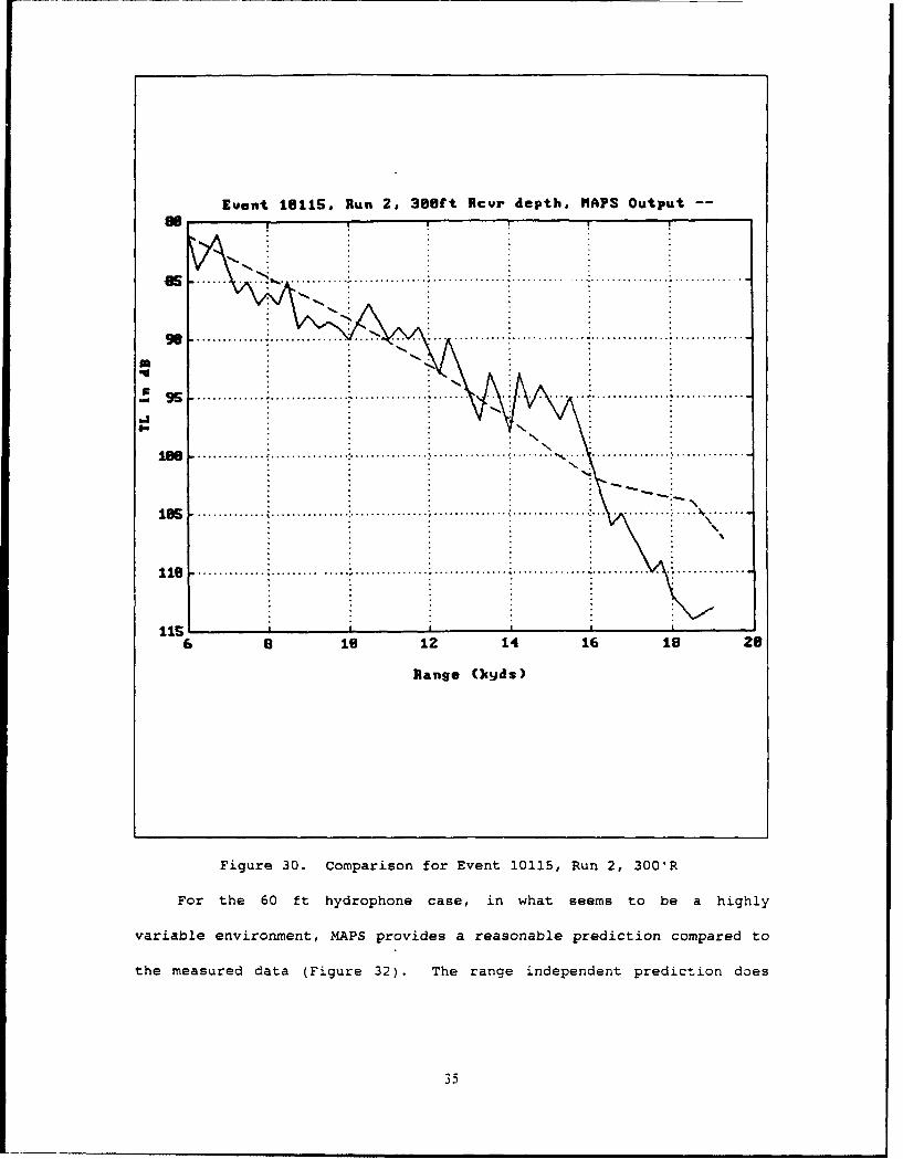
For the 60 ft hydrophone case, in what seems to be a highly
variable environment, MAPS provides a reasonable prediction compared to
the measured data (Figure 32). The range independent prediction does
35
ZEent 16115. Run 3, 25f t Rcur depth, NAPS Output -- vs 21
"7 5 - . . .% . ,.. . ........ ;................................ .. .. .. .. .......................... ........
so B ........... ............... •........... ... .. -, .... . ............. .. ....... .. ..... ........... ........
INDEPENDENT
5 19 15 28 25
Range (kyds)
Figure 31. Comparison for Event 10115, Run 3, 25'R
36
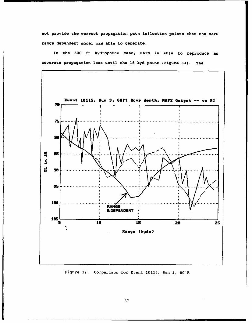
not provide the correct propagation path inflection points that the MAPS
range dependent model was able to generate.
In the 300 ft hydrophone case, MAPS is able to reproduce an
accurate propagation loss until the 18 kyd point (Figure 33). The
luent 18115. Run 3. 60St Rcvr depth. MAPS Output -- ue I178
75...................... .............................................
S........................................... ........ .............
l g .. . . ...... .... ..... . .... ... ./ .. ........... ........... :-::...."" ' "
bi /85 .......... °°
RANGE
INDEPENDENT
18515 18 15 28 25
Range Chidz)
Figure 32. Comparison for Event 10115, Run 3, 601R
37
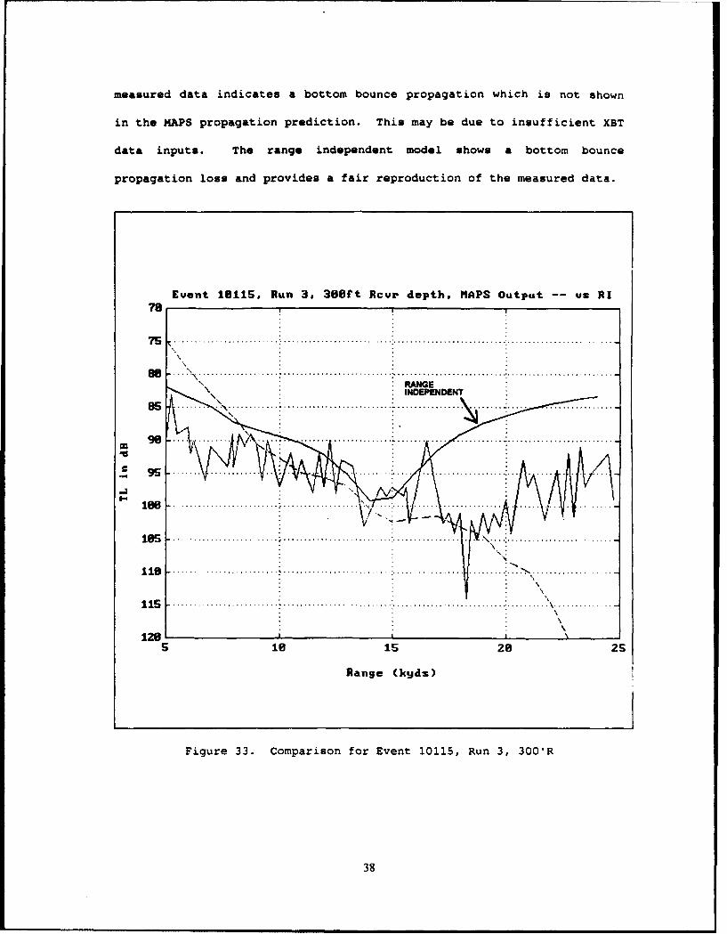
measured data indicates a bottom bounce propagation which is not shown
in the MAPS propagation prediction. This may be due to insufficient XBT
data inputs. The range independent model shows a bottom bounce
propagation loss and provides a fair reproduction of the measured data.
Euent 18115, Run 3, 38Sft Rcui depth, MAPS Output -- us RI78
a s . . .:• . . . . . . . ............................................................ .........................\ RANGE
•. \\INDEPEDENT
7. .........................
1 1 8 . .......................... ............... ........... ................. ....... .. . •.... ..... . . . . . . .
.~ 95
128'115 ' ... ...
128 \5 18 15 20 25
Range (kyda)
Figure 33. Comparison for Event 10115, Run 3, 300'R
38
VI. CONCLUSIONS AND RECO1EKDATIONS
The results that have been presented show that MAPS has the
potential to produce an accurate propagation loss prediction in the
littoral shallow water regions. What is meant by potential is that if
high resolution environmental inputs along the acoustic path of interest
are obtained an accurate propagation loss prediction can be made.
Certain SHAREM measurements illustrated that the environment was
changing in an hour period during the run. The SHAREM measurements
strongly emphasizes the point that continuous efforts must be made to
gather temporal/spatial XBT when operating in shallow water
environments. During SHAREM 102 propagation measurements, a single XBT
at own ship position did not possess the data necessary to predict what
the propagation loss would be 25 kyd down range. Another critical
environmental input for accurate littoral propagation loss prediction is
the bottom loss input. As the SHAREM 102 propagation loss measurements
show, the standard data of MGS 7 resulted in very high propagation loss
predictions. Without the in situ SHAREM 102 calculation of bottom loss,
the MAPS propagation loss predictions would not have been in the "ball
park" for the bottom bounce propagation loss predictions. Also a range
independent model cannot account for the environmental changes along the
acoustic path of interest to accurately predict the propagation loss as
it can provide highly inaccurate results that may cause the tactical
commander to use incorrect tactics in a littoral shallow water
environment.
39
MAPS has shown that in a littoral shallow water region that the
resolution of the bathymetry can be an important factor in obtaining an
accurate propagation loss prediction. MAPS' SAAAB high resolution data
base has enhanced the prediction capability.
MAPS has illustrated that with accurate environmental inputs that
accurate propagation loss can be provided to the tactical user. The
amount of data that is needed to provide useful propagation loss
predictions would present a problem for the Anti-Submarine Warfare
Commander. No longer can a CV Battle Group designate a single XBT guard
ship for obtaining all environmental data for ASW prosecution. In
littoral shallow water regions it becomes the responsibility of all
assets in the group to obtain as much environmental data as possible
given the tactical situation. Helicopters must play a major role in
this gathering process since they are the only asset that can proceed
down the threat bearing and obtain XBT data and relay the data back in
real time.
Another problem exists that must be addressed with the inputs of
environmental data to MAPS. The process must change from a stand alone
acoustic prediction system where each ship obtains its own XBT data and
manually inputs the XBT in MAPS, to a system that can link from
helicopter to ship to ship so that the XBT data can be used and
transferred by the group in a real time manner. In addition, better
user friendly software must be implemented that provide semi-automatic
assistance to the MAPS operator that allows the decision as to where the
boundaries should extend for a specific or group of XBTs. This XBT use
assessment must be accomplished on a temporal/spatial basis in the
littoral environment as the SHAREM 102 propagation loss measurements
40

have shown. This capability must occur before MAPS will become a useful
tactical tool to the Anti-Submarine Warfare Commander.
41
LIST OF REBFAIIUCBS
1. Huggins, Jeff A., Investigation of a Tactical Active Multi-Environment Acoustic Prediction System, M.S. Thesis, NavalPostgraduate School, Monterey, CA, 1992.
2. Naval Undersea Warfare Center Division Newport Report 68,Prooaoation Loss Measurements In The Gulf of Oman, by P. Abbot, D.Morton and I. Dyer, April 1993.
3. Naval Undersea Warfare Center Detachment New London Report 931077,Gulf Of Oman Environmental Study, by E. M. Podeszwa, 30 June 1993.
42
APPENDIX A
135 DR 195
W2 DRI 145REBRNTS)
143
APPENDIX B
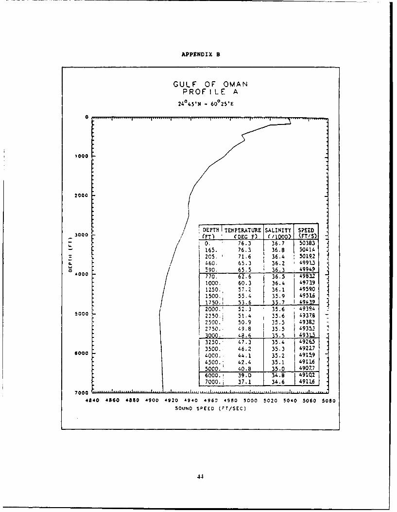
GULF OF OMANPROFILE A
2445*N - 60 0 25'E
1000
2000
00T/ ?PTH TEMPERATURE INITYtI
-- 5O •/ i(FT) (DEC F) (/1000)| (FT/S)
-- F165. 76.3 36.8 5041!4
205. 71.6 36.4 5019,2460. 65.3 36.2 4991.3
'6000 390. 65.5 36.3 4994 ]770. 62.6 36.5 1 498321000. 60.3 36 .4 497191250. 57.2 36.1 4959.01500.1 55.4 3!.9 4951.61750.i 53.6 35.7 49419
L 2000.' 52.3 35.6 4939t4o000 2250.: 51.4 35.6 49378
2500. 50.9 35.5 4938"2750.- 49.8 35.5 493-33000.. 48.6 I,35.5 4931.63250.' 47.3 I35.4 4920.3500.; 46.2 I 35.3 492V7
6004000., 44.1 35*2 491',94500.* 42.4 35.1 491L65000. 40.8 35.0 490776000.' 39.0 34.8 491Q2
7000. __37.1 34.6 4911U6 47000 ................. . t ..... .. ... ...,I.........
4840 4860 4880 4900 4920 4940 4960 4980 5000 5020 5040 5060 5080SOUND SPEED (7T/SEC)
44
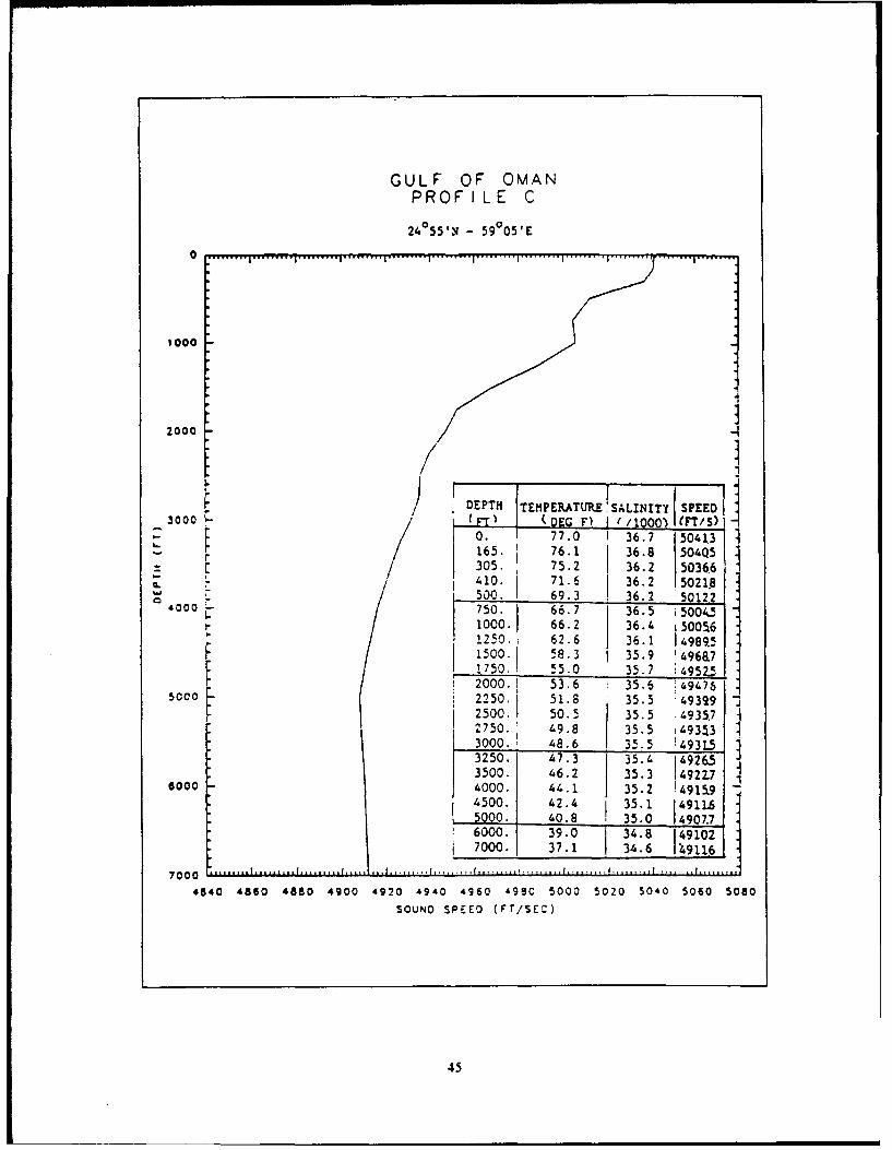
GULF OF OMANPROFILE C
24 055'N - 59°05'E
100
2000
F) DEPTH TEMPERATURE;SALINITY SPEED300 ,FD (DEG F) I r/100oo0•~(FT/S)
0. 77.0 1 36.7 15041.3165. 76.1 36.8 504Q5r. 305. 75.2 36.2 5036.6
/ 410. 71.6 36.2 5021.500. 69.3 36.2 50122
,000 c 750. 66.7 36.5 i5004.51000. 66.2 36.4 1500U61250. 62.6 36.1 14989.51500. 58.3 35.9 '496a71_750. 55.0 35.7 i4952.52000. 53.6 1 35.6 49476
Sco 2250. 51.8 35.5 :49329C 2500. 50.5 35.5 4935.7
2750. 49.8 35.5 i493533000. 48.6 35.5 !493L53250. 47.3 35.4 492653500. 46.2 35.3 49217
6000 4000. 44.1 35.2 !:4915A4500. 42.4 35.1 4911.65000. 40.8 35.0 49077S6000. 39.0 34.8 149102
7000. 37.1 34.6 49116,
7000 ......4840 4860 4880 4900 4920 4940 4960 498C 5000 5020 50A0 5060 5080
SOUND SPEED (FT/SEC)
45
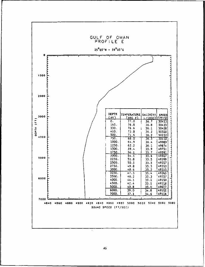
GULF OF OMAN
PROFILE E
250 05'N . 59 0 05'E
0 . . . . I.. . . . ......... I ........ I . .......... I.......
1000
2000
DEPTH TEMPERATURE SALINITY SPEED3000 r) r D LG F) t/loo) I(FT/S)
0. 77.0 36.7 50413i165. 76.8 36.8 50415330. 76.6 36.1 504ZO8410. 73.a 36.2 503ZD500. 71.6 36.2 502124000 750. 68.0 36.5 -0ilO
1000. 64.9 36.4 499491 1250. 62.2 36.1 498741 1500. 59.4 35.9 4975I
1750. 56.1 35.7 4959i2000. 54.1 35.6 495Q75000 2250. 51.8 35.5 4939.92500. 50.5 35.5 493172750. 49.8 35.5 493533000. 48.6 35.5 .4931.53250. 47.3 35.4 '4926.53500. 46.2 35.3 492Z7
6000 4000. 44.1 35.2 491194500. 42.4 35.1 4911.5000. 40.8 35.0 490A776000. 39.0 f 34.8 491qz7000. 37.1 34.6 4911.6
7000 ......... ....... .... 1 .
4840 4860 4850 4900 4920 4940 4960 4980 5000 5020 5040 5060 5080
SOuND SPEED (FTr/SEC)
46
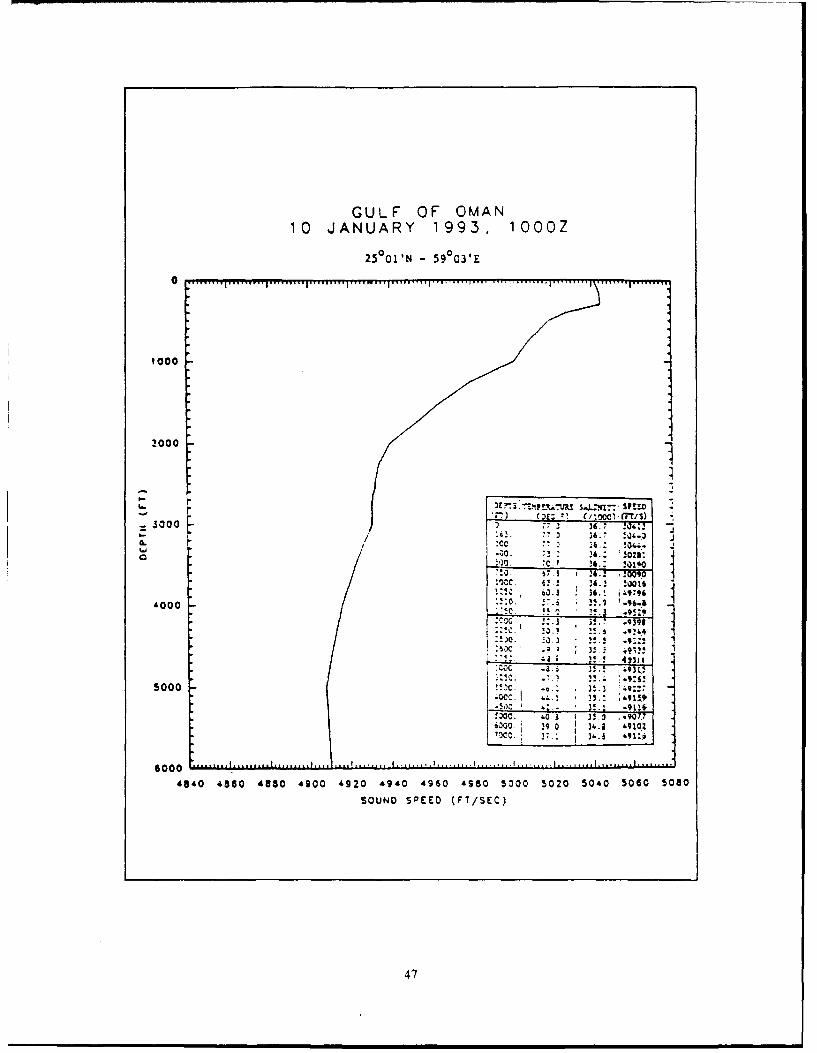
GULF OF OMAN10 JANUARY 1993. 1000Z
25 01'N - 59°03*E
0 ... ... f i l .... .. II 1 .... 1 .... 1 1.... I 1........... I. . . . .
1000
2000
- (I .oo ).t ris)U= .•oa • lri ..:! ]• o,
/3000 2 . : 3 6. * !, -
i6.: !•OI.
.6: 5022:
.. 0
;g•,. ""' 1o.! .!00161oo¢, 6 .l 36.!. i-'9-96".•,0 .=:. • j,..) T 96. .
4000 .C -0•• .•.. P '..;•496.1
3!.;
5000 i 3L
:;o. "0.• 3 !.•; -9.161 9 - -o I 3!I W71.1
'0cc. .: .• ,)• ' ,,;.. ' * • '. i:.- .
6000 , . .......... . ........ - I I .
4540 4850 4880 4900 4920 4940 4960 'S80 5000 5020 5040 506C 5080
SOUND SPEED (FT/SEC)
47
TEMPERATURE (C)
10 12 14 16 18 20 22 24 26
100
200
300.....
700....... ...... ........ ..................
DEPTH
500
800 I , ==
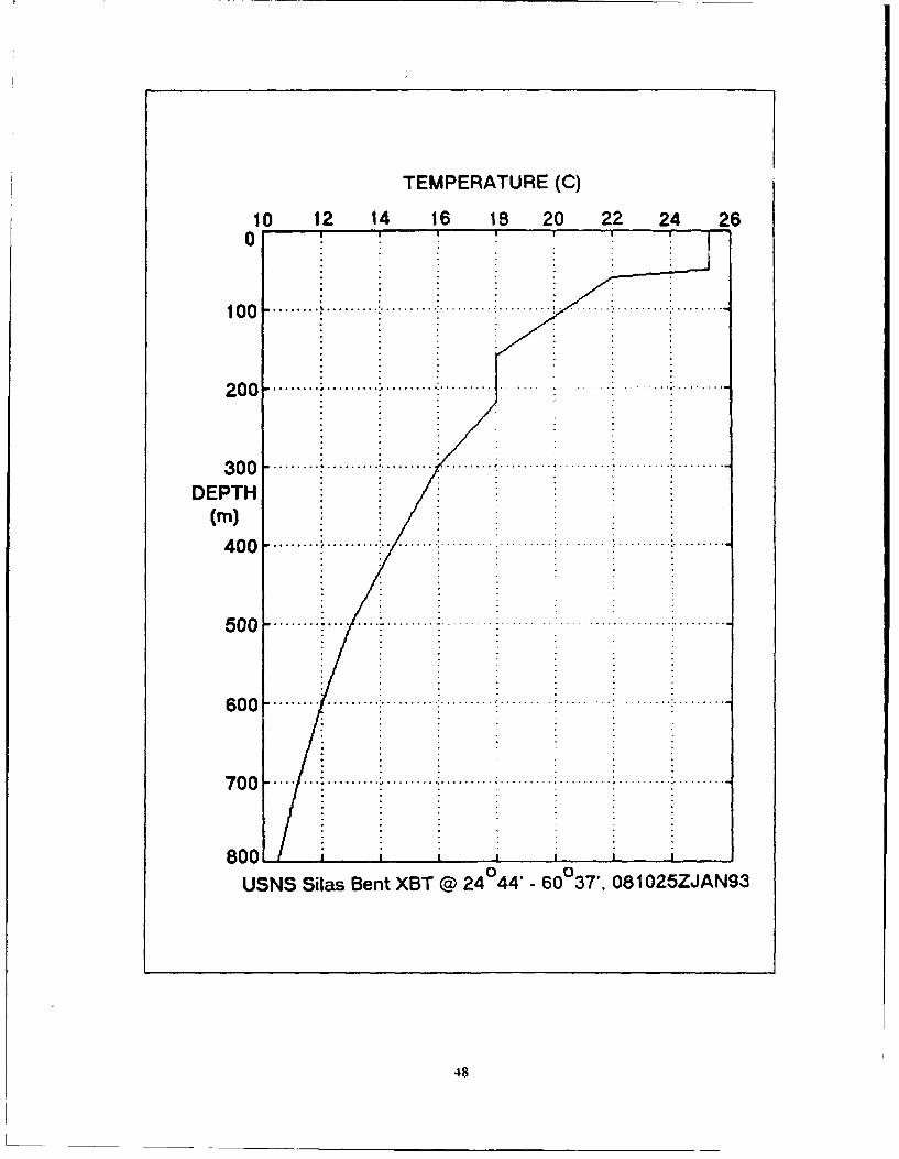
USNS Silas Bent XBT @ 24044' - 60 0 37', 081025ZJAN93
48
TEMPERATURE (C)
10 12 14 16 18 20 22 24 26
0
100 .......................... ......... .......... ........
200 ..... * ......................... .......
DEPTH
(in ) . . . . .. . . .. . . . . .. . . . . ... . . .. . . . . . . . . . . . .
400 ............ % ............. ......... ......500
600
700
800 1 , I I I,
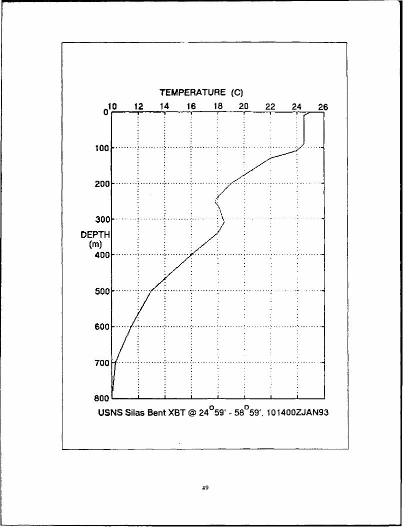
USNS Silas Bent XBT @ 24059' - 58059', 101400ZJAN93
49
TEMPERATURE (C)
6 8 10 12 14 16 18 20 22 24 260 .
200.. . ..................... ...............200 ... ...
400 ........................................ ........ .......
DEPTH .
(M)
600 .................... ............
800 ........................... ...... ..................
1000
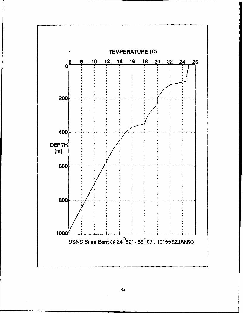
USNS Silas Bent @ 24o52' - 59007', 101556ZJAN93
50

TEMPERATURE(F)62 64 66 68 70 72 74 76 780
0 0 ................................... ............... ...................... . .
DEPTH
600 ..................................................... .....
80. ................. ...... .......................
800 .......
1000 .....................................................
1200 .
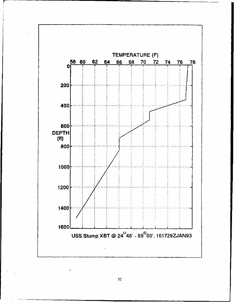
USS Stump XBT @ 24052' - 59009'. 101629Z93
51
TEMPERATURE (F)58O60 62 646668 70 72 74 7678
1600 I
UDEtmPTH©2U4,-5O0~1072ZA9
(ft2
TEMPERATURE (C)
10 12 14 16 18 20 22 24 26
0
100............................... ...................... .. ...
200. ... ............... ................... ......... .......200-
300.................. ...............
DEPTH(in)
40...... .. ......... .... ........... .......
500...... : .............. ....... ........... . . . . .
600 .......................................
700 L
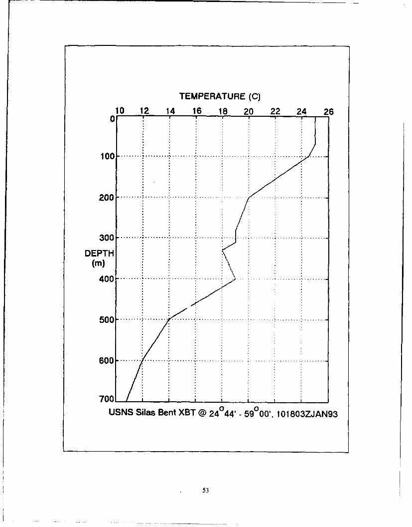
USNS Silas Bent XBT @ 24044' - 59000'. 101803ZJAN93
53
TEMPERATURE (F)
62 64 66 68 70 72 74 76 78
200.
400 ........ ...... ......................................400
DEPTH(ft) .
B0O ............. .......... ..... ......... ...................
800 ........................................... ..............
1000
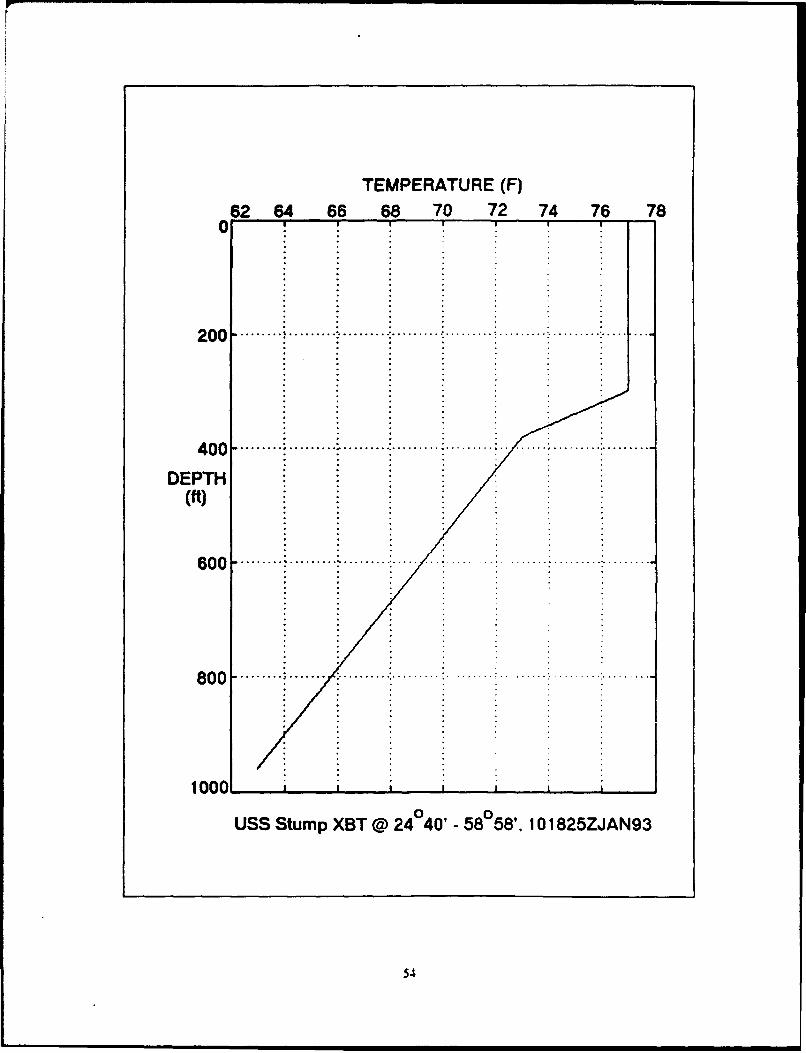
USS Stump XBT @ 24040' - 58058'. 101825ZJAN93
54
APPENDIX C
Es
+ +
Be
+ +
+ +)
10 + +
Se+ +
, !
150 1 L . . .L. . . . ... .
RANGE (+,'. -S.i
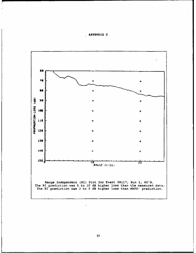
Range Independent (RI) Plot for Event 08117, Run 1, 601R.The RI prediction was 5 to 10 dB higher loss than the measured data.
The RI prediction was 3 to 5 dB higher loss than MAPS' prediction.
55
+-
+ +
li 96 + +
12 - + +
-ji 126 +
136 + +
14e + +
ID 2DRANCE (KYDEF.
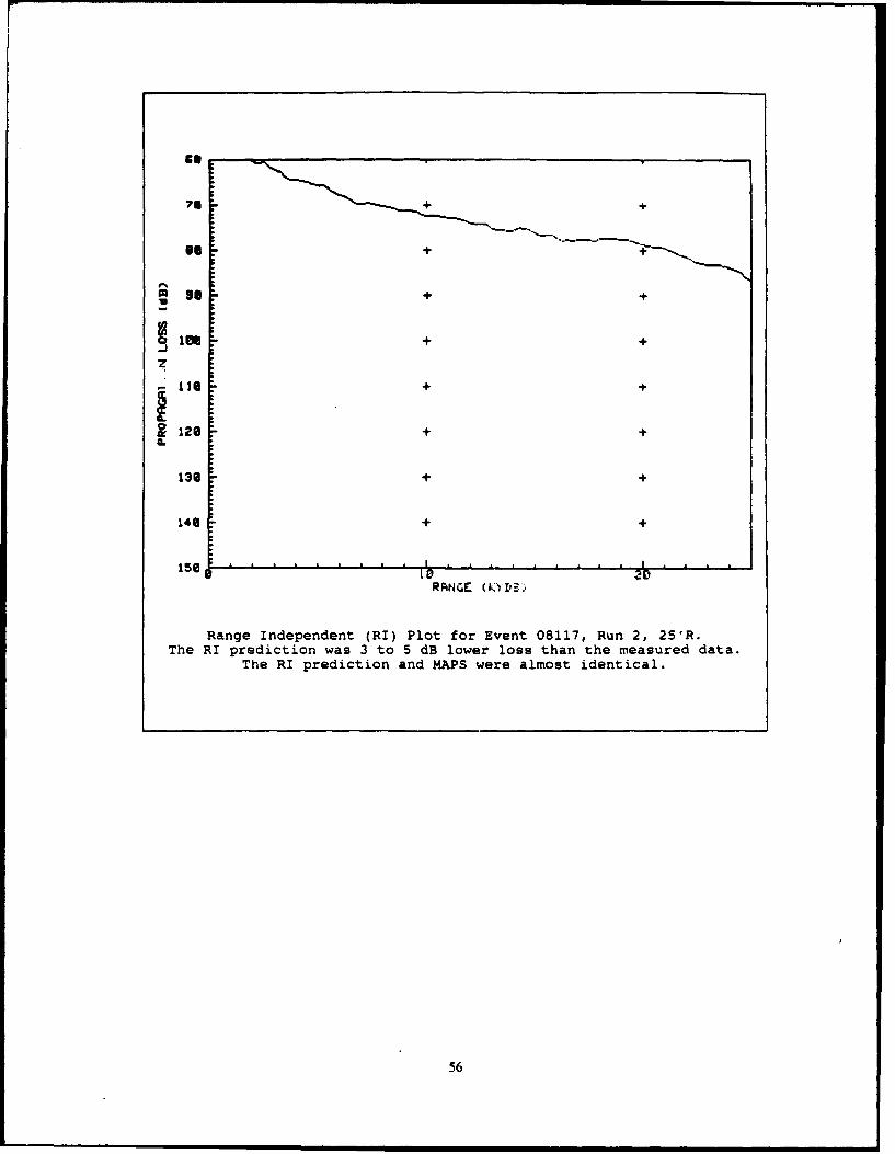
Range Independent (RI) Plot for Event 08117, Run 2, 25'R.The RI prediction was 3 to 5 dB lower loss than the measured data.
The RI prediction and MAPS were almost identical.
56
GE+
+ +
Its - ++
13a + +
1403 + +
15 1a .. . . . . . . . iý . . . . . . . . . 2 . . .
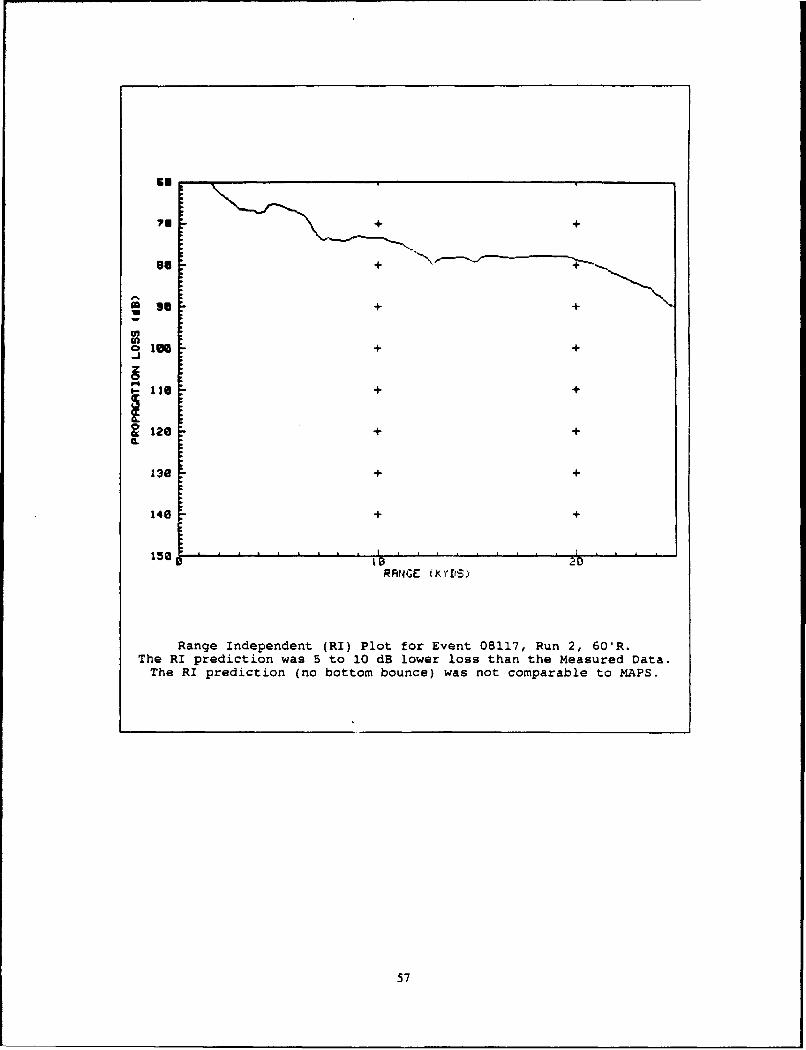
Range Independent (RI) Plot for Event 08117, Run 2, 60'R.The RI prediction was 5 to 10 dB lower loss than the Measured Data.
The RI prediction (no bottom bounce) was not comparable to MAPS.
57
73 + +
m **+ +ie3 + +
1 2e + +
13e + +
149 + +
ISO . . . . . . . . . i ' . . .' ' - .- ,' , ,
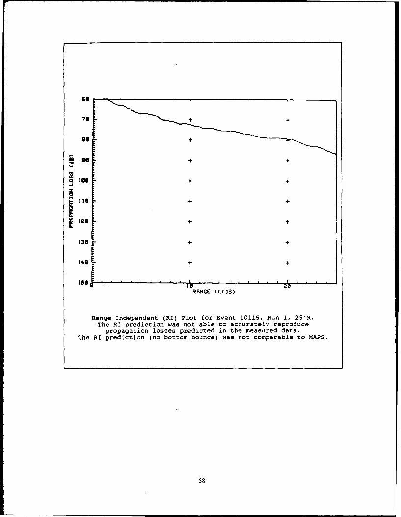
RANCE (KYD')
Range Independent (RI) Plot for Event 10115, Run 1, 25'R.The RI prediction was not able to accurately reproduce
propagation losses predicted in the measured data.The RI prediction (no bottom bounce) was not comparable to MAPS.
58
7. + +9
+6 +
U, + +
13l6 + +
J•120 ++
U,.
130 + +
14+ +
156 6 , I , , I , , , .,ID 2D
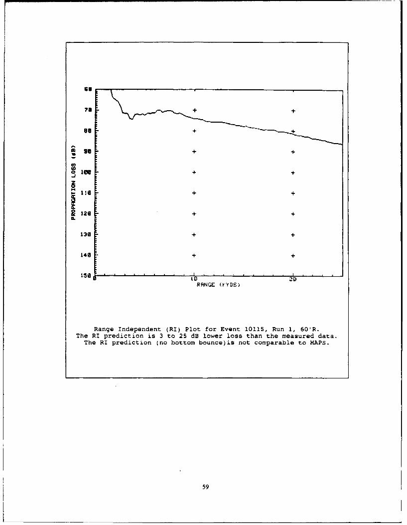
RF4NCGE (t:YDSJ
Range Independent (RI) Plot for Event 10115, Run 1, 60'R.The RI prediction is 3 to 25 dB lower loss than the measured data.
The RI prediction (no bottom bounce)is not comparable to MAPS.
59
7t + +
10 + +
tie + +
12e + +
130 + +
146 + +
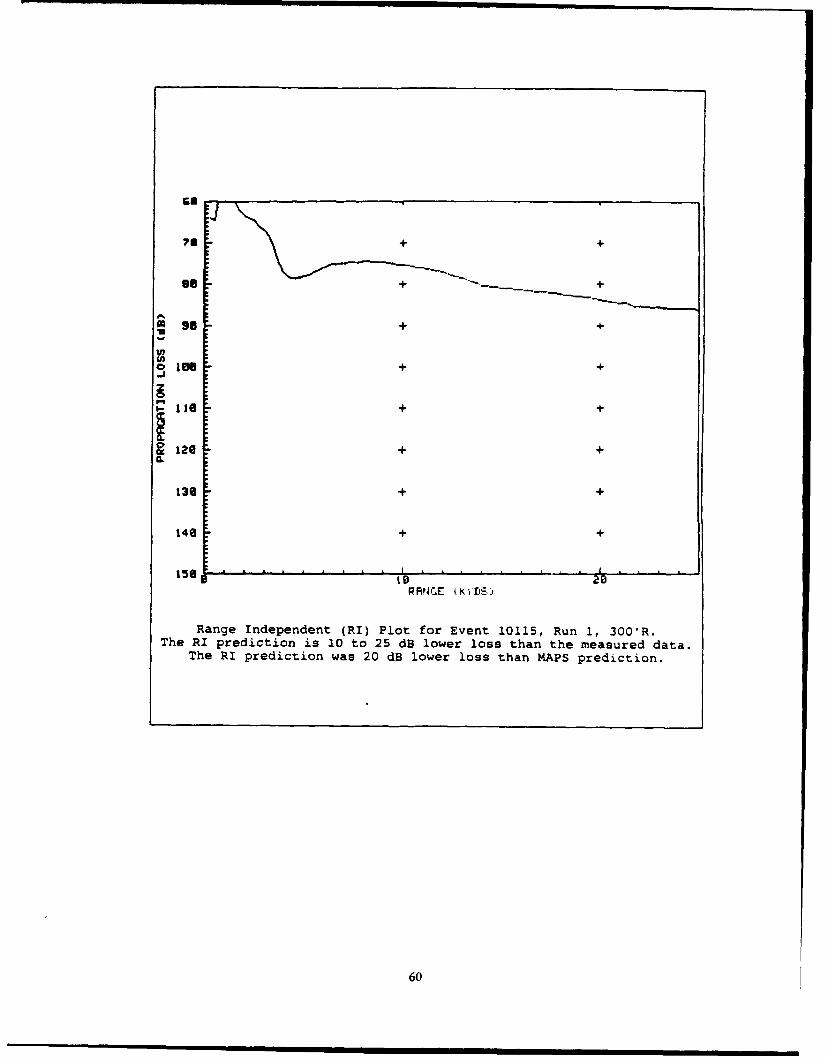
156 0PlANCiE ( K",'DS:)
Range Independent (RI) Plot for Event 10115, Run 1, 300'R.The RI prediction is 10 to 25 dB lower loss than the measured data.
The RI prediction was 20 dB lower loss than MAPS prediction.
60
S+ +
SI +
s 96 + +
toCA0106 + +
D..Il116 + +
R 1206 + +.
136 + +
140 + +
150 b . . . . .i .I . . : 'E'PRNGE (KDS',
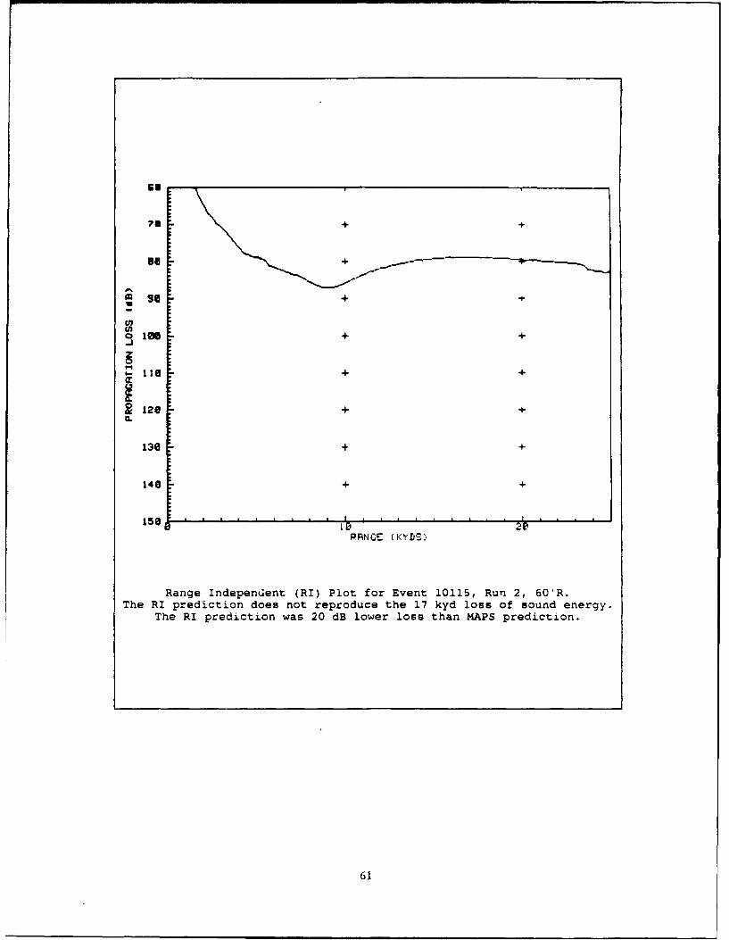
Range Independent (RI) Plot for Event 10115, Run 2, 60'R.The RI prediction does not reproduce the 17 kyd loss of sound energy.
The RI prediction was 20 dB lower loss than MAPS prediction.
61
'U
71 + +
++
S9 + +
1 me+ +-J
I le + +
Z120 + +Q.
136 + +
140 + +
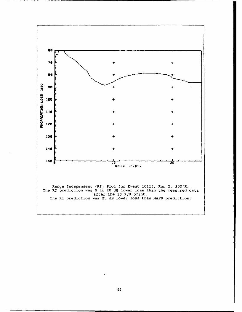
Range Independent (RI) Plot for Event 10115, Run 2, 300'R.The RI prediction was 5 to 20 dB lower loss than the measured data
after the 10 kyd point.The RI prediction was 25 dB lower loss than MAPS prediction.
62
KU
7I + +
so +
om lea:- + -• -+
Ilei +1 +
912 + +
nCL
130 + +
140 + +
150 . . . . . . . . L . . . . . . 2 ,RANIE (K•£1S'.
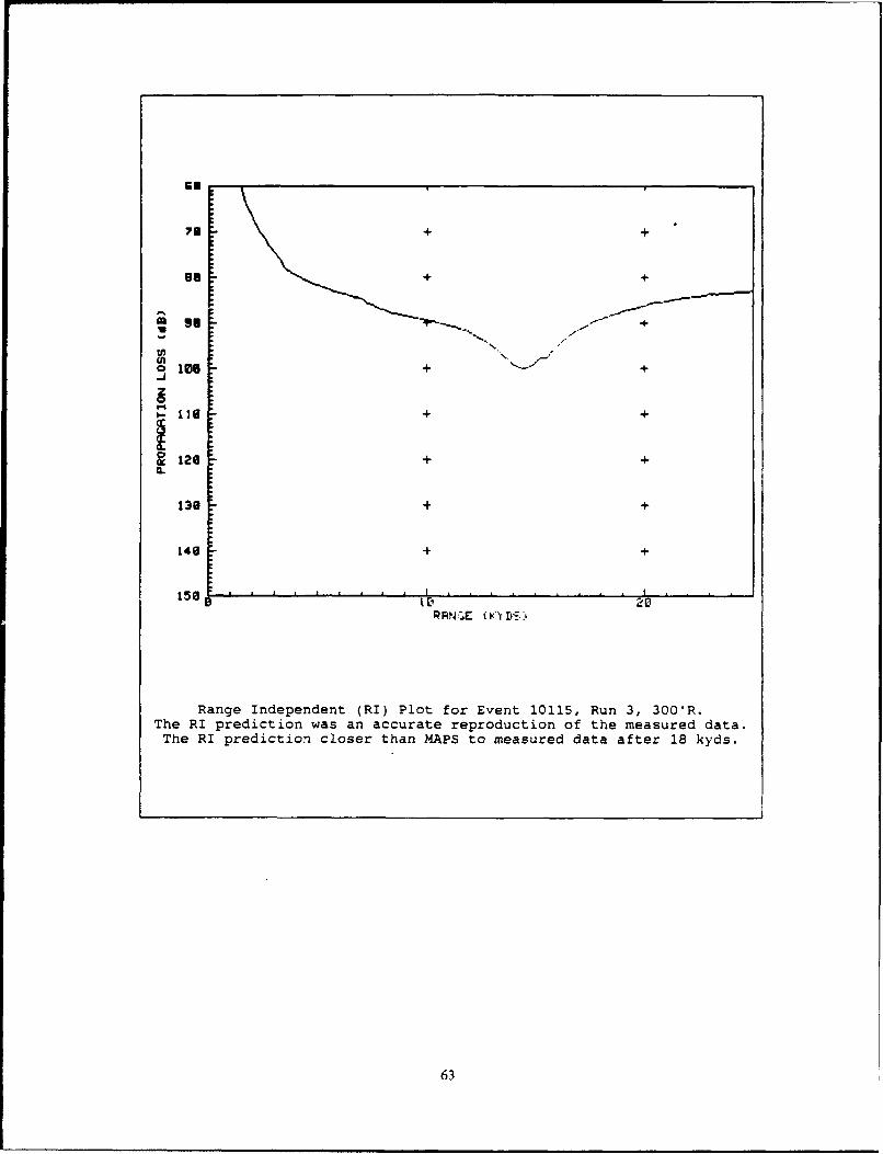
Range Independent (RI) Plot for Event 10115, Run 3, 300'R.The RI prediction was an accurate reproduction of the measured data.
The RI prediction closer than MAPS to measured data after 18 kyds.
63
INITIAL DISTRIBUTION LIST
No. Copies1. Defense Technical Information Center 2
Cameron StationAlexandria VA 22304-6145
2. Library, Code 052 2Naval Postgraduate SchoolMonterey CA 93943-5002
3. The Johns Hopkins University 2Applied Physics LaboratoryJohns Hopkins RdAttn: Chris Vogt 7-322Laurel, MD 20723-6099
4. Commanding Officer 1Naval Research Laboratory4555 Overlook Avenue, S.W.Washington, D.C. 20375
5. Commanding Officer 1Naval Undersea Warfare Center DetachmentNew London, CT 06320-5594
6. Department of the Navy 1Program Executive Officer for Undersea WarfareWashington, D.C. 20362-5169
7. Director, Submarine Warfare Division (N87) IChief of Naval OperationsWashington, DC 20350-2000
8. Department of the Navy 1
Attn: PMO-411Program Executive Officer for Undersea WarfareWashington, DC 20362-5169
9. Commander 1Surface Warfare Development Group2200 Amphibious DriveNorfolk, VA 23521-2850
10. Commander 1Surface Warfare Development GroupAttn: CAPT John Seeley2200 Amphibious DriveNorfolk, VA 23521-2850
64
11. Dr Michael J. Pastore128 Monte Vista DriveMonterey, CA 93940
12. Mr Steve DassingerNaval Undersea Warfare Center DetachmentNew London, CT 06320-5594
65