NAVAL POSTGRADUATE SCHOOLdtic.mil/dtic/tr/fulltext/u2/a427120.pdfNAVAL POSTGRADUATE SCHOOL September 2004 ... Advantage of Stealth Fighter over Conventional Fighter ... Polar Plot

NAVAL POSTGRADUATE

SCHOOL

MONTEREY, CALIFORNIA

THESIS

Approved for public release; distribution is unlimited

DEVELOPMENT OF CODE FOR A PHYSICAL OPTICS RADAR CROSS SECTION PREDICTION AND ANALYSIS

APPLICATION

by

Filippos Chatzigeorgiadis

September 2004

Thesis Co-Advisors: David C. Jenn D. Curtis Schleher

THIS PAGE INTENTIONALLY LEFT BLANK

i

REPORT DOCUMENTATION PAGE Form Approved OMB No. 0704-0188 Public reporting burden for this collection of information is estimated to average 1 hour per response, including the time for reviewing instruction, searching existing data sources, gathering and maintaining the data needed, and completing and reviewing the collection of information. Send comments regarding this burden estimate or any other aspect of this collection of information, including suggestions for reducing this burden, to Washington headquarters Services, Directorate for Information Operations and Reports, 1215 Jefferson Davis Highway, Suite 1204, Arlington, VA 22202-4302, and to the Office of Management and Budget, Paperwork Reduction Project (0704-0188) Washington DC 20503. 1. AGENCY USE ONLY (Leave blank)

2. REPORT DATE September 2004

3. REPORT TYPE AND DATES COVERED Master’s Thesis

4. TIT LE AND SUBTITLE: Development of Code for a Physical Optics Radar Cross Section Prediction and Analysis Application 6. AUTHOR(S) Filippos Chatzigeorgiadis

5. FUNDING NUMBERS

7. PERFORMING ORGANIZATION NAME(S) AND ADDRESS(ES) Naval Postgraduate School Monterey, CA 93943-5000

8. PERFORMING ORGANIZATION REPORT NUMBER

9. SPONSORING /MONITORING AGENCY NAME(S) AND ADDRESS(ES) N/A

10. SPONSORING/MONITORING AGENCY REPORT NUMBER

11. SUPPLEMENTARY NOTES The views expressed in this thesis are those of the author and do not reflect the official policy or position of the Department of Defense or the U.S. Government. 12a. DISTRIBUTION / AVAILABILITY STATEMENT Approved for public release; distribution is unlimited

12b. DISTRIBUTION CODE

13. ABSTRACT (maximum 200 words) The significance of the Radar Cross Section (RCS) in the outcome of military engagements makes its prediction an

important problem in modern Electronic Warfare. The POFACETS program, previously developed at the Naval Postgraduate School (NPS), uses the Physical Optics method to predict the RCS of complex targets, which are modeled with the use of tri-angular facets. The program has minimum computer resource requirements and provides convenient run–times. This thesis up-graded, enhanced and expanded the functionalities and capabilities of the POFACETS program. The new functionalities were implemented by upgrading the Graphical User Interface and model database, allowing the creation of models with an unlimited number of facets, providing capabilities for the automatic creation of models with standard geometric shapes, allowing the combination of existing target models, providing capabilities for sharing target models with commercial CAD programs, and creating new display formats for RCS results. The new computational capabilities include the development of a user–updateable database of materials and coatings that can be applied to models in one or multiple layers, and the computation of their effects on the models’ RCS. Also implemented are the computations of the ground’s effect on the RCS, and the exploita-tion of symmetry planes in models, in order to decrease run–time for RCS prediction.

15. NUMBER OF PAGES

149

14. SUBJECT TERMS Physical Optics, Radar Cross Section, Monostatic, Bistatic, Electromagnetic Scattering, Graphical User Interface, Faceted Models

16. PRICE CODE

17. SECURITY CLASSIFICATION OF REPORT

Unclassified

18. SECURITY CLASSIFICATION OF THIS PAGE

Unclassified

19. SECURITY CLASSIFICATION OF ABSTRACT

Unclassified

20. LIMITATION OF ABSTRACT

UL

NSN 7540-01-280-5500 Standard Form 298 (Rev. 2-89) Prescribed by ANSI Std. 239-18

ii


iii

Approved for public release; distribution is unlimited

DEVELOPMENT OF CODE FOR A PHYSICAL OPTICS RADAR CROSS SECTION PREDICTION AND ANALYSIS APPLICATION

Filippos Chatzigeorgiadis Major, Hellenic Air Force

B.S., Hellenic Air Force Academy, 1990

Submitted in partial fulfillment of the requirements for the degree of

MASTER OF SCIENCE IN SYSTEMS ENGINEERING and

MASTER OF SCIENCE IN ELECTRICAL ENGINEERING

from the

NAVAL POSTGRADUATE SCHOOL September 2004

Author: Filippos Chatzigeorgiadis

Approved by: David C. Jenn

Thesis Co-Advisor

D. Curtis Schleher Thesis Co-Advisor

John P. Powers Chairman, Department of Electrical and Computer Engineering

Dan C. Boger Chairman, Department of Information Sciences

iv


v

ABSTRACT The significance of the Radar Cross Section (RCS) in the outcome of military en-

gagements makes its prediction an important problem in modern Electronic Warfare. The

POFACETS program, previously developed at the Naval Postgraduate School (NPS),

uses the Physical Optics method to predict the RCS of complex targets, which are mod-

eled with the use of triangular facets. The program has minimum computer resource re-

quirements and provides convenient run–times. This thesis upgraded, enhanced and ex-

panded the functionalities and capabilities of the POFACETS program. The new func-

tionalities were implemented by upgrading the Graphical User Interface and model data-

base, allowing the creation of models with an unlimited number of facets, providing ca-

pabilities for the automatic creation of models with standard geometric shapes, allowing

the combination of existing target models, providing capabilities for sharing target mod-

els with commercial CAD programs, and creating new display formats for RCS results.

The new computational capabilities include the development of a user–updateable data-

base of materials and coatings that can be applied to models in one or multiple layers, and

the computation of their effects on the models’ RCS. Also implemented are the computa-

tions of the ground’s effect on the RCS, and the exploitation of symmetry planes in mod-

els, in order to decrease run–time for RCS prediction.

vi


vii

TABLE OF CONTENTS

I. INTRODUCTION........................................................................................................1 A. MOTIVATION ................................................................................................1 B. BACKGROUND ..............................................................................................2 C. STATEMENT OF PURPOSE ........................................................................3 D. DELIMITATIONS OF THE PROJECT.......................................................5 E. THESIS OVERVIEW .....................................................................................5

II. RADAR CROSS SECTION THEORY.....................................................................7 A. RADAR CROSS SECTION AND THE RADAR EQUATION ..................7 B. SIGNIFICANCE OF THE RADAR CROSS–SECTION ............................8 C. RADAR CROSS SECTION DEFINED.......................................................11 D. SCATTERING REGIONS............................................................................14

1. Low Frequency Region or Rayleigh Region 2

1Lπλ

<<

..............14

2. Resonance Region or Mie Region 2

1Lπλ

≈

.................................14

3. High Frequency Region or Optical Region 2

1Lπλ

>>

................14

E. RADAR CROSS SECTION PREDICTION METHODS..........................15 1. Method of Moments ...........................................................................15 2. Finite Difference Methods .................................................................16 3. Microwave Optics ..............................................................................16 4. Physical Optics ...................................................................................17

F. SUMMARY....................................................................................................17

III. PHYSICAL OPTICS APPLIED TO TRIANGULAR FACET MODELS ..........19 A. RADIATION INTEGRALS FOR FAR ZONE SCATTERED FIELDS..19 B. RADIATION INTEGRALS FOR A TRIANGULAR FACET .................20 C. RADIATION INTEGRALS FOR A TRIANGULAR FACET .................22 D. COORDINATE TRANSFORMATIONS ....................................................24 E. PHYSICAL OPTICS SURFACE CURRENT COMPUTATION ............26 F. SCATTERED FIELD COMPUTATION ....................................................27 G. DIFFUSE FIELD COMPUTATION ...........................................................29 H. TOTAL FIELD FROM A TARGET ...........................................................31 I. SUMMARY....................................................................................................33

IV. NEW FUNCTIONALITIES ADDED TO THE POFACETS PROGRAM..........35 A. GRAPHICAL USER INTERFACE (GUI) UPGRADE TO

CURRENT MATLAB VERSION ................................................................35 1. Rationale .............................................................................................35 2. Procedure ............................................................................................36

viii

3. Results .................................................................................................36 B. MODEL DATABASE UPGRADE...............................................................38

1. Rationale .............................................................................................38 2. Procedure ............................................................................................39 3. Results .................................................................................................39

C. MANUAL MODEL DESIGN .......................................................................40 1. Rationale .............................................................................................40 2. Procedure ............................................................................................41 3. Results .................................................................................................44

D. GRAPHICAL MODEL DESIGN.................................................................45 1. Rationale .............................................................................................45 2. Procedure ............................................................................................46 3. Results .................................................................................................50

E. IMPORT/EXPORT OF MODELS ..............................................................51 1. Rationale .............................................................................................51 2. Procedure ............................................................................................52 3. Results .................................................................................................53

F. COMBINATION OF MODELS...................................................................56 1. Rationale .............................................................................................56 2. Procedure ............................................................................................56 3. Results .................................................................................................58

G. RCS COMPUTATION OPTIONS...............................................................60 1. Rationale .............................................................................................60 2. Procedure and Results .......................................................................61

a. RCS versus Observation Angles .............................................61 b. RCS versus Frequency............................................................68

H. RCS RESULTS DISPLAY OPTIONS.........................................................70 1. Rationale .............................................................................................70 2. Procedure and Results .......................................................................70

a. User–Selectable Dynamic Range............................................70 b. Polar Plots...............................................................................71 c. Combination Plots...................................................................72

I. SUMMARY....................................................................................................76

V. NEW COMPUTATIONAL CAPABILITIES ADDED TO THE POFACETS PROGRAM.................................................................................................................77 A. EXPLOITATION OF SYMMETRY PLANES ..........................................77

1. Rationale .............................................................................................77 2. Background ........................................................................................77 3. Procedure ............................................................................................81 4. Results .................................................................................................84

B. EFFECTS OF MATERIALS AND COATINGS ON RCS........................85 1. Rationale .............................................................................................85 2. Background ........................................................................................86

a. Case 1: Multiple Composite Layers........................................87 b. Case 2: Composite Layer on PEC ..........................................89

ix

c. Case 3: Composite Layer ........................................................90 d. Case 4: Multiple Layers on PEC............................................90

3. Procedure ............................................................................................91 4. Results .................................................................................................94

C. EFFECTS OF GROUND ..............................................................................98 1. Rationale .............................................................................................98 2. Background ........................................................................................99 3. Procedure ..........................................................................................104 4. Results ...............................................................................................105

D. SUMMARY..................................................................................................107

VI. SUMMARY AND RECOMMENDATIONS.........................................................109 A. SUMMARY..................................................................................................109 B. RECOMMENDATIONS.............................................................................110

APPENDIX. POFACETS FILES AND MODEL DATABASE STRUCTURE............111 A. POFACETS FILE FRAMEWORK ...........................................................111 B. POFACETS FILE DESCRIPTION ...........................................................119 C. POFACETS DATA STRUCTURES DESCRIPTION .............................122

1. Model File Structure ........................................................................122 a. Coord .....................................................................................122 b. Facet ......................................................................................122 c. Scale.......................................................................................122 d. Symplanes..............................................................................122 e. Comments..............................................................................122 f. Matrl ......................................................................................123

2. Material Database File Structure ...................................................123 a. Name......................................................................................123 b. er ............................................................................................123 c. tande.......................................................................................123 d. mpr.........................................................................................123 e. m2pr .......................................................................................123

LIST OF REFERENCES ....................................................................................................125

INITIAL DISTRIBUTION LIST.......................................................................................127

x


xi

LIST OF FIGURES

Figure 1. Typical Radar–Target Scenario (From Ref. 5.) .................................................7 Figure 2. Advantage of Stealth Fighter over Conventional Fighter (After Ref. 1.) ........10 Figure 3. Coordinate System (After Ref. 5.) ...................................................................12 Figure 4. Radar Cross Section of a Sphere (From Ref. 5.)..............................................15 Figure 5. Far Field Scattering from an Arbitrary Body (After Ref. 2.). ..........................19 Figure 6. Arbitrary Oriented Facet (After Ref. 3.). .........................................................21 Figure 7. Arbitrary Oriented Facet (a) Geometry (b) Facet Sub–Areas (From Ref.

3.). ....................................................................................................................22 Figure 8. Global and Local Coordinate Systems (From Ref. 3.).....................................24 Figure 9. Rotation Angles (From Ref. 3.). ......................................................................25 Figure 10. Gaussian Approximation of a Rough Surface (From Ref. 3.) .........................30 Figure 11. (a) Large Correlation Distance, (b) Small Correlation Distance (From Ref.

3.) .....................................................................................................................31 Figure 12. Flow Chart for the RCS Calculation of a Collection of Facets........................33 Figure 13. POFACETS Main Screen ................................................................................37 Figure 14. POFACETS Contributors ................................................................................38 Figure 15. File Conversion Options (circled)....................................................................40 Figure 16. Manual Model Design GUI Form....................................................................41 Figure 17. Vertex Coordinate Input ...................................................................................42 Figure 18. Facet Definition................................................................................................43 Figure 19. Plate Model Display.........................................................................................44 Figure 20. Dart Model Display..........................................................................................45 Figure 21. Graphical Model Design GUI Form................................................................46 Figure 22. Sphere Parameters............................................................................................47 Figure 23. Sphere Model (20 Points per Circle) ...............................................................47 Figure 24. Sphere Model (40 Points per Circle) ...............................................................48 Figure 25. Model Rotation Dialog Box.............................................................................49 Figure 26. (a) Cone Model, (b) Rotation of 60 Degrees Around X Axis..........................49 Figure 27. Graphically Designed Models (a) Ellipsoid, (b) Fuselage, (c) Ogive, (d)

Box...................................................................................................................51 Figure 28. Import/Export Options (circled).......................................................................53 Figure 29. Cylinder Model Imported from Stereo–Lithographic Format .........................54 Figure 30. T–62 AFV Model Imported from ACADS Format .........................................54 Figure 31. X–29 Aircraft Model Imported from DEMACO Format ................................55 Figure 32. Star–Shaped Model Imported from Pdetool ....................................................55 Figure 33. Model Combination (circled)...........................................................................56 Figure 34. UAV Model......................................................................................................57 Figure 35. Facet Descriptions............................................................................................58 Figure 36. Various Models (a) X–29, (b) AIM–9, (c) AGM–84 ......................................59 Figure 37. Armed X–29 Aircraft Model............................................................................60 Figure 38. Monostatic RCS Calculation GUI ...................................................................63

xii

Figure 39. RCS of a 1 m by 1 m PEC Plate at 1 GHz, TM wave, for φ =0 ......................64 Figure 40. RCS of a 1 m by 1 m PEC Plate for at 1 GHz, TM Wave ...............................65 Figure 41. Bistatic RCS Calculation GUI .........................................................................66 Figure 42. Bistatic RCS Example ......................................................................................67 Figure 43. Specular Reflection and Forward Scatter from a Plate ....................................67 Figure 44. Monostatic RCS versus Frequency GUI ..........................................................68 Figure 45. RCS of a 1 m by 1 m PEC Plate versus Frequency (Vertical Incidence) ........69 Figure 46. Bistatic RCS versus Frequency GUI................................................................69 Figure 47. Dynamic Range Effects ...................................................................................71 Figure 48. Polar Plot..........................................................................................................72 Figure 49. Combination Plot .............................................................................................73 Figure 50. Combination Graph of the UAV Model ..........................................................74 Figure 51. Annotated UAV RCS Plot ...............................................................................75 Figure 52. Symmetry Plane Scenario – Global Coordinates .............................................78 Figure 53. Symmetry Plane Scenario – Local Coordinates...............................................79 Figure 54. Cases of Incidence Angle in Local Coordinates ..............................................80 Figure 55. Symmetry Controls in the Graphical Model Design GUI (circled).................81 Figure 56. Symmetry Plane Definition..............................................................................82 Figure 57. Symmetry Planes for a Sphere Model .............................................................83 Figure 58. Symmetry Selection for Monostatic RCS Calculations (circled) ....................84 Figure 59. Monostatic RCS of a Sphere with Radius of 3 m at 18 GHz...........................85 Figure 60. Wave Incident on Multiple Layers (After Ref. 8.)...........................................87 Figure 61. Incidence and Transmission Angles at the Boundary Between Two Layers...89 Figure 62. Composite Layer on PEC.................................................................................90 Figure 63. Materials Database Management GUI .............................................................91 Figure 64. New Material Data Input GUI .........................................................................91 Figure 65. Material Application GUI ................................................................................92 Figure 66. Material View GUI ..........................................................................................93 Figure 67. Material Type Selection Dialog Box ...............................................................93 Figure 68. RCS vs. Frequency of a 1 m by 1 m PEC Plate (normal incidence)................94 Figure 69. RCS vs. Frequency of a 1 m by 1 m Plate with One Composite Layer

(normal incidence) ...........................................................................................95 Figure 70. RCS vs. Frequency of a 1 m by 1 m Plate with Two Composite Layers

(normal incidence) ...........................................................................................96 Figure 71. RCS vs. Frequency of a 1 m by 1 m Plate with One Composite Layer on

PEC (normal incidence)...................................................................................97 Figure 72. RCS vs. Frequency of a 1 m by 1 m Plate with Two Composite Layers on

PEC (normal incidence)...................................................................................98 Figure 73. Target Over Infinite Ground Plane ..................................................................99 Figure 74. Direct Incident – Direct Scattered..................................................................100 Figure 75. Direct Incident – Reflected Scattered ............................................................101 Figure 76. Reflected Incident – Direct Scattered ............................................................102 Figure 77. Reflected Incident – Direct Scattered Equivalent Scenario ...........................102 Figure 78. Reflected Incident – Reflected Scattered .......................................................103 Figure 79. Reflected Incident – Reflected Scattered Equivalent Scenario ......................103

xiii

Figure 80. Ground Plane Controls (circled) ....................................................................105 Figure 81. RCS vs. Frequency of a 1 m by 1 m PEC Plate (normal incidence)..............106 Figure 82. RCS vs. Frequency of a 1 m by 1 m PEC Plate (normal incidence) with

PEC Ground Plane 9.25 m Below the Plate...................................................106 Figure 83. POFACETS Main Screen File Framework....................................................112 Figure 84. Manual Model Design File Framework .........................................................113 Figure 85. Graphical Model Design File Framework .....................................................114 Figure 86. Monostatic RCS Calculation File Framework ...............................................115 Figure 87. Bistatic RCS Calculation File Framework.....................................................116 Figure 88. Utilities File Framework ................................................................................117 Figure 89. RCS Computation and Display File Framework ...........................................118

xiv


xv

ACKNOWLEDGMENTS

The author is grateful to his country, Greece, and the Hellenic Air Force for pro-

viding him with the opportunity to study at the Naval Postgraduate School.

The author would also like to acknowledge with sincere gratitude the advice, help,

guidance and encouragement he received from Professor David C. Jenn during the nine

months that led to the conclusion of this thesis.

Many thanks are also due to Professors D. Curtis Schleher, Phillip E. Pace, A. W.

Cooper, and Roberto Cristi for making his studies at NPS a truly worthwhile learning ex-

perience.

The author would like to also thank his wife, Effrosyni, and his daughter, Niki, for

their tireless patience, enduring understanding and unfailing support.

He is also thankful of his parents for encouraging his to improve himself con-

stantly through education and personal study.

xvi


xvii

EXECUTIVE SUMMARY

Signature control, one of the most significant aspects of Electronic Warfare,

places great emphasis on the reduction of RF signatures emitted from military platforms.

One important aspect in RF signature reduction involves the Radar Cross Section (RCS)

of the platforms. The goal of the RCS reduction is to decrease the range at which an en-

emy radar can detect the platform, in order to minimize the reaction time available to the

threat or to deny detection altogether, by allowing the platform to remain “hidden” in the

ground or sea clutter.

Thus, the prediction of the Radar Cross Section of operational platforms and the

evaluation of the effects of potential RCS reduction techniques, such as shaping and use

of radar absorbing materials (RAM), for the full spectrum of usable radar frequencies

provides a challenging problem in modern electronic warfare. The POFACETS 2.3 pro-

gram, a MATLAB application, developed at the Naval Postgraduate School, is an inex-

pensive, user–friendly, easy to use, RCS prediction software tool that has minimum re-

quirements on computer resources and is capable of producing RCS predictions within

small amounts of time for standard three–dimensional geometric shapes.

The program models any arbitrary target by utilizing triangular facets. The scat-

tered field from each facet is computed using the radiation integrals. The Physical Optics

method is used to calculate the currents on each facet. This method is a high frequency

approximation that provides the best results for electrically large targets as well as in the

specular direction.

The need to improve the program was dictated by certain inherent limitations in

the target modeling, the structure of the file models, and some compatibility issues with

the current MATLAB version. Hence, the objective of this thesis was to improve the ex-

isting POFACETS RCS prediction software tool. This objective was achieved by provid-

ing new functionalities and adding new computational capabilities to the POFACETS 2.3

version.

xviii

The new functionalities included the Graphical User Interface (GUI) and model

database upgrade, the improvement of the manual model design options, the creation of a

graphical model design GUI, the inclusion of capabilities for importing and exporting

models compatible with commercial Computer Aided Design (CAD) programs, the in-

clusion of capabilities for a combination of existing models, the computation of RCS ver-

sus frequency, and the creation of new options for the display of RCS results.

The new computational capabilities included the exploitation of symmetry planes

in target models to decrease run–time for RCS prediction, the development of a user-

updateable database of materials, which can be applied to models in one or multiple lay-

ers, the computation of the effects of materials and coatings in the model RCS, and the

computation of the effects of the ground on the RCS of a model.

Overall, the program is now user–friendlier, by providing easy–to–use GUIs and

familiar controls, while minimizing the possibility for erroneous input. Moreover, the

creation of complex models was facilitated through the use of automated standard model

design and the new capabilities, which allow the program to combine existing models and

share models with CAD software. Despite the new improvements and computational ca-

pabilities, minimal effect occurred to the required program execution time, while the op-

tion for the exploitation of symmetry planes, when these exist, can drastically decrease

execution time.

The versatility of the program was enhanced by allowing the capability for RCS

computation versus frequency and providing a broader range of options for RCS display.

Indeed, these capabilities allow for the use of the program not only for RCS prediction,

but for RCS analysis as well.

Finally, the capability to use very complex models, the materials database, the ca-

pability to apply different types of materials and coatings to the models’ surfaces and the

inclusion of the effects of the ground on RCS, have made the POFACETS 3.0 a much

more useful tool regarding real–world RCS prediction and analysis problems.

xix

The POFACETS 3.0 program was implemented in the current version of the

MATLAB software, and thus, it can be easily modified and upgraded through the wide

variety of tools provided by this software package. Two areas of potential improvements

involve including additional scattering mechanisms, such as second reflections, diffrac-

tion, and traveling waves in the RCS calculations and providing capabilities for importing

a wider variety of model file types from commercial CAD software.

xx


1

I. INTRODUCTION

A. MOTIVATION

Signature control is recognized today as one of the most significant aspects of

Electronic Warfare. In the past decades, signature control technology, commonly known

as stealth, has become a critical technology area, as it directly affects the survivability of

both the military weapon platforms and the weapons themselves. The goal of signature

control is to reduce the various signatures of a platform to a level that allows the platform

to remain undetected from the threat sensors.

In the effort to produce such low–observable platforms, various signatures can be

considered, such as RF (Radio Frequency), IR (Infrared), visible, laser, acoustic and

magnetic. However, in general, the RF signatures are considered to be of prime impor-

tance in military applications, because radar is the premier military sensor today and is

capable of providing reliable target detection at long ranges and under a wide variety of

environmental conditions (Ref. 1).

Consequently, the reduction of the RF signature has received high priority in the

design of many new military platforms (e.g., F-117 and B-2 aircraft, the Swedish Navy’s

Visby Class Stealth Corvette, etc.). One aspect of the reduction of the RF signatures in-

volves the reduction of emissions. Indeed, if a high–power radar is operating aboard a

platform, its emissions will probably be detected by the enemy’s passive sensors, such as

the electronic support measures (Ref. 2). The other aspect of the reduction of the RF sig-

natures involves the Radar Cross Section (RCS) of the platforms. The goal of the RCS

reduction is to decrease the range at which an enemy radar can detect the platform, in or-

der to minimize the reaction time available to the threat or to deny detection altogether,

by allowing the platform to remain “hidden” in the ground or sea clutter.

Thus, the prediction of the Radar Cross Section of operational platforms and the

evaluation of the effects of potential RCS reduction techniques, such as shaping and use

of radar absorbing materials (RAM) for the full spectrum of usable radar frequencies

provides a challenging problem in modern electronic warfare. One approach to high fre-

2

quency RCS prediction calculations is to describe a complex model with an array of sim-

ple shapes, such as triangles or flat plates. The contribution of each simple shape is calcu-

lated in order to obtain the RCS of the whole target.

Although several RCS prediction methods exist for arbitrary three–dimensional

targets, most of them require a considerable amount of computer resources and process-

ing time. In addition, the procurement of the software, which implements these methods,

usually represents a significant amount of investment in capital and training time. Hence,

there is a need for an inexpensive, user–friendly, easy to use, RCS prediction software

tool that will run on a standard computer and will be able to produce RCS predictions

within small amounts of time (in the order of seconds or minutes) for standard three–

dimensional geometric shapes. This software tool should also provide the user the capa-

bility to model any three–dimensional object with simple component shapes, display the

geometry of the model in order to allow inspection by the user and, of course, allow the

user to enter the necessary parameters for the calculation of the Radar Cross Section of

the model.

B. BACKGROUND

Such a software code was developed by Professor David C. Jenn and Commander

Elmo E. Garrido Jr. The code was implemented in MATLAB and utilizes the Physical

Optics (PO) approximation technique for the RCS calculation. This technique, as ex-

plained in Chapter II, is not overly computationally demanding and provides relatively

accurate results for most large target models, while requiring minimal amounts of run–

time. The initial RCS prediction code was developed by Professor David C. Jenn. Com-

mander Elmo J. Garrido Jr. upgraded the code by adding Graphical User Interface (GUI)

capabilities (Ref. 3). The end–product is the POFACETS program, whose current version

is 2.3.

The POFACETS program provides the user an easy–to–use GUI that allows the

input of all necessary parameters, while preventing erroneous data input and other user

errors. The program enables the user to create a model comprised of triangular facets,

with options for specifying various surface characteristics of the facets, such as surface

resistivity, surface roughness and whether a facet side is external (hence potentially il-

lumi-

3

nated by the threat radar) or internal (hence not illuminated). The program allows the user

to display and inspect the model and it provides additional options for enhancing the

visualization of its geometry.

Once a model is defined, the user can calculate its RCS, defined in the next chap-

ter, based on the radar frequency and other parameters of interest. Once the RCS is com-

puted, an appropriate plot is generated to display the calculated data.

The main disadvantages of the existing POFACETS version are related to its

model design features. Specifically, the GUI allows the user to enter a limited number of

facets (40 maximum) making it impossible to model more complex objects. At the same

time, since the program requires the coordinates of each vertex of a facet to be entered

manually, the whole process can become time consuming and counter–productive for lar-

ger models. In addition, there is no capability to combine existing models to create ones

that are more complex or to import models created in other commercially available Com-

puter Aided Design (CAD) programs.

Finally, since the POFACETS 2.3 version was developed in 2000, in a previous

version of MATLAB, this creates maintenance and compatibility problems with the cur-

rent MATLAB versions, especially in the area of the GUI figure definition.

C. STATEMENT OF PURPOSE

The purpose of this thesis was to enhance the existing POFACETS RCS predic-

tion software tool. It exploits the existing RCS calculation code and aims to achieve the

following two goals.

The first is to improve the existing functionalities of the POFACETS 2.3 version

by:

• Upgrading the GUI to the current MATLAB version

• Upgrading the POFACETS models database

• Providing capabilities for the creation of models with an arbitrary number of facets (limited only by the computer capabilities)

• Providing capabilities for the automatic creation of models with standard geometric shapes

• Allowing the combination/merging of existing target models

4

• Providing capabilities for importing models created in commercially available CAD programs

• Providing capabilities for exporting models, so that they can be used by commercially available CAD programs

• Providing new options for computing RCS versus frequency

• Providing new display options of RCS results, such as polar plots, and RCS plots superimposed on the model geometry

The second is to add new computational capabilities to the program. These in-

clude:

• Exploitation of symmetry planes in target models to decrease run–time for RCS prediction

• Computation of the RCS of a model over infinite ground plane

• Development of a user–updateable database of materials which can be ap-plied to models in one or multiple layers

• Computation of effects of materials and coatings in the model RCS

The existing POFACETS version is already in use by NPS students, students of

other universities and RCS professionals. This thesis is expected to provide new capabili-

ties regarding the prediction of RCS and to make the application even more versatile and

easy to use. Specifically:

• The added capabilities (e.g., RCS of targets over ground planes, effects of materials and coatings) will make the existing application a serious cand i-date for use not only by universities for educational purposes but by other services and institutions.

• The versatility of the application will be greatly enhanced by adding the capability to import target models designs implemented in other CAD software. Similarly, the capability to combine and merge existing target models will provide the option to create very complex target models by combining simpler models of subcomponents designed by different ind i-viduals or students.

• The application will become even more user–friendly by upgrading the ex-isting Graphical User Interface, adding a database of materials and coat-ings that the user can choose from and providing the capability to use cer-tain standard model shapes (e.g., spheres, plates, boxes, cylinders, ellip-soids, trapezoids, cones, radomes, fuselages, etc.).

5

D. DELIMITATIONS OF THE PROJECT

This thesis will aim to expand, enhance and upgrade the current POFACETS

software version. The existing core software code of this program, which produced the

calculation of the scattered field from a triangular facet for a given set of parameters, also

formed the basis of the new POFACETS version, which resulted from this thesis. All the

new features, options, functionalities, and capabilities that this thesis added to the

POFACETS program utilized this code at some point in the program.

This delimitation makes also clear that the program is based exclusively on the

Physical Optics approximation method for the calculation of the RCS of a model. Chapter

II discusses the limitations and weaknesses of this method.

Furthermore, during the design, development and implementation of the code,

which implements the new functionalities and capabilities of the new POFACETS ve r-

sion, certain assumptions or approximations will have to be made, in order to limit the

program complexity and to produce acceptable run–times. When these assumption or ap-

proximations occur, the appropriate section in the following chapters of this thesis ex-

plains their rationale.

E. THESIS OVERVIEW

This chapter provides a brief background regarding the need for an inexpensive

and easy–to–use software tool for the prediction of the Radar Cross Section of complex

models, along with the features that such a tool should incorporate. The statement of pur-

pose and the detailed goals of this project have been specified and its delimitations de-

scribed.

Chapter II describes the importance of the radar cross–section, as this appears in

the radar equation and provides a practical example of its significance in a military en-

gagement. The RCS is then formally defined, followed by a brief discussion regarding

electromagnetic scattering fundamentals. The chapter concludes with a comparative dis-

cussion of some common methods of RCS prediction.

Chapter III contains the theoretical framework of the Physical Optics approxima-

tion method and the mathematical formulations used in the POFACETS program to im-

plement this method. All the auxiliary tools and formulas utilized in the program are de-

6

fined and explained. The prediction of the scattered field from a single facet is first ex-

plained and then it is used as the basis for the calculation of the scattered field from a col-

lection of facets (i.e., an arbitrary model). Essentially, this chapter contains the funda-

mental theory utilized in the existing POFACETS version.

Chapter IV contains the description of the new functionalities of the POFACETS

version resulting from this thesis work. It provides the details of the available options for

the manual or graphical design of a model, the capabilities for importing models from, or

exporting models to, other commercially available CAD software, the description of

available RCS computation options and the available RCS results display options.

Chapter V presents the new RCS computation capabilities added to the

POFACETS program as a result of this thesis. These include the calculation of the effects

of infinite ground planes on target RCS, the calculation of the effects of various materials

and coatings, and the exploitation of symmetry planes. For each case, the theoretical

framework upon which the software is based is presented, followed by the implemented

program features and the RCS results obtained.

Chapter VI summarizes the outcomes of the thesis work and suggests further im-

provements to the program.

Finally, since the end result of this thesis work is quite a complex program, con-

sisting of more than 30 MATLAB script files and 15 MATLAB figure files, the Appen-

dix at the end of the thesis provides the framework that shows the interconnection and

functionality of each script or figure file. The main goal of this framework is to help the

reader understand how the program operates, rather than providing a user manual, since

the program itself incorporates detailed user instructions either through dialog boxes or

help screens.

7

II. RADAR CROSS SECTION THEORY

This chapter discusses the importance of the Radar Cross Section and its role in

the radar equation and provides examples of its significance in Electronic Warfare. The

RCS is then formally defined, followed by a brief discussion regarding scattering regions.

The chapter concludes with a comparative discussion of some common methods of RCS

prediction.

A. RADAR CROSS SECTION AND THE RADAR EQUATION

The radar equation relates the range of a radar to the characteristics of the trans-

mitter, the receiver, the antennas, the target, and the environment. It is useful for deter-

mining the maximum range at which a given radar can detect a target and it can serve as a

means for understanding the factors that affect radar performance (Ref. 4).

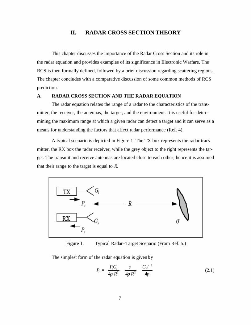
A typical scenario is depicted in Figure 1. The TX box represents the radar trans-

mitter, the RX box the radar receiver, while the grey object to the right represents the tar-

get. The transmit and receive antennas are located close to each other; hence it is assumed

that their range to the target is equal to R.

Figure 1. Typical Radar–Target Scenario (From Ref. 5.)

The simplest form of the radar equation is given by

2

2 24 4 4t t r

r

PG GP

R Rλσ

π π π =

(2.1)

8

where, Pr is the power received by the radar (in watts), Pt the output power of the trans-

mitter (in watts), Gt the gain of the transmitter antenna, Gr the gain of the receiver an-

tenna, σ the Radar Cross Section of the target (in m2), λ the wavelength of the radar’s

operating frequency (in meters) and R the range between the radar and the target (in me-

ters).

Notice that the first term in parenthesis represents the radar power density at the

target (in watts/m2). The product of the first and second terms in parenthesis represents

the power density at the radar receiver due to the reflection or scattering that occurs on

the target. The third term in parenthesis represents the amount of the reflected power cap-

tured by the receiving antenna aperture.

For the monostatic radar case, in which the radar uses the same antenna for

transmitting and receiving, Gt is equal to Gr and by setting Gt = Gr = G, Equation (2.1)

can be written as:

2 2

3 4(4 )t

rPG

PR

σλπ

= . (2.2)

The maximum range of a radar, maxR , is the distance beyond which the target

cannot be detected. It occurs when the received signal power Pr just equals the minimum

detectable signal minS (Ref. 4). Substituting minrP S= in Equation (2.2) and rearranging

terms gives:

1 /42 2

max 3min(4 )

tPGR

Sσλ

π

=

. (2.3)

Although this form of the radar equation excludes many important factors and usually

predicts high values for maximum range, it depicts the relationship between the maxi-

mum radar range and the target’s RCS.

B. SIGNIFICANCE OF THE RADAR CROSS–SECTION

Equation (2.3) indicates that the free–space detection range of a radar is propor-

tional to the RCS of the target, raised to the one–quarter power ( )1 /4σ . Thus, decreasing

the RCS by a factor of 10 translates to a 56% decrease in the free–space detection range.

Consequently, the reaction time of the weapon system that utilizes this radar will be de-

9

creased to approximately half. In addition, if the target is an aircraft flying at low altitude

in heavy clutter, the MTI improvement factor required for detection will be increased by

10 dB, rendering many radars designed to detect conventional aircraft inoperable (Ref.

1).

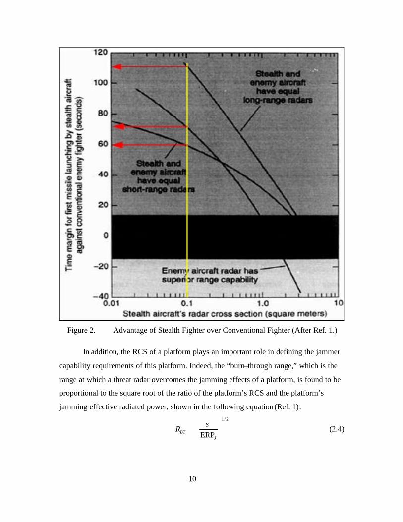
An illustration of the effectiveness of RCS in military engagements is depicted in

Figure 2. In this scenario, a “stealth” fighter with RCS that varies from 0.01 m2 to 10 m2

is engaged head on with a conventional fighter aircraft, whose RCS is 5 m2. The engage-

ment occurs at 30,000 feet and both aircraft fly at Mach 0.9. Three different curves are

shown. One curve corresponds to an engagement scenario in which both aircraft have

long–range radars capable of detecting a target with RCS of 5 m2 at 125 km. The second

curve corresponds to an engagement scenario in which both aircraft have short–range ra-

dars capable of detecting a target with RCS of 5 m2 at 50 km. The third curve corresponds

to an engagement scenario in which the “stealth” fighter has a radar with a 90-km detec-

tion range against a target with RCS of 5 m2, while the conventional fighter has a long–

range radar capable of detecting the same target at 125-km range (Ref. 1).

The shaded area in the middle of the graph represents a region in which either

fighter can fire the first missile shot. It is easy to see that as the RCS of the “stealth” air-

craft is reduced and that the margin for the first missile launch by this aircraft against the

conventional fighter is increased. For example, if the “stealth” aircraft has a RCS of 0.1

m2, then it could target the conventional fighter for approximately 60 seconds, before the

conventional fighter can fire its missiles (for the equal short–range radar scenario). This

time margin exceeds 70 seconds in the scenario in which the conventional fighter is

equipped with a superior range radar and reaches approximately 110 seconds in the sce-

nario in which both aircraft have equal long–range radars.

10

Figure 2. Advantage of Stealth Fighter over Conventional Fighter (After Ref. 1.)

In addition, the RCS of a platform plays an important role in defining the jammer

capability requirements of this platform. Indeed, the “burn–through range,” which is the

range at which a threat radar overcomes the jamming effects of a platform, is found to be

proportional to the square root of the ratio of the platform’s RCS and the platform’s

jamming effective radiated power, shown in the following equation (Ref. 1):

1 /2

ERPBTJ

Rσ

∝

(2.4)

11

where BTR is the burn–through range and ERPJ is the jammer’s effective radiated power.

It is clear that, for the same jamming effect (i.e., the same burn–through range), if the tar-

get RCS (σ ) is decreased then the self–protection jammer effective radiated power can

be decreased in the same proportion. Eventually, as the Radar Cross Section becomes

small enough, no jammer is required. Thus, the term ( /ERP )Jσ can be considered a fig-

ure of merit for the jammer (Ref. 1).

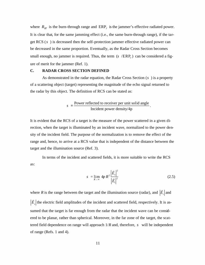
C. RADAR CROSS SECTION DEFINED

As demonstrated in the radar equation, the Radar Cross Section (σ ) is a property

of a scattering object (target) representing the magnitude of the echo signal returned to

the radar by this object. The definition of RCS can be stated as:

Power reflected to receiver per unit solid angle

Incident power density/4pσ ≡ .

It is evident that the RCS of a target is the measure of the power scattered in a given di-

rection, when the target is illuminated by an incident wave, normalized to the power den-

sity of the incident field. The purpose of the normalization is to remove the effect of the

range and, hence, to arrive at a RCS value that is independent of the distance between the

target and the illumination source (Ref. 3).

In terms of the incident and scattered fields, it is more suitable to write the RCS

as:

2

22lim 4

s

Ri

ER

Eσ π

→∞=

r

r (2.5)

where R is the range between the target and the illumination source (radar), and iEr

and

sEr

the electric field amplitudes of the incident and scattered field, respectively. It is as-

sumed that the target is far enough from the radar that the incident wave can be consid-

ered to be planar, rather than spherical. Moreover, in the far zone of the target, the scat-

tered field dependence on range will approach 1/R and, therefore, σ will be independent

of range (Refs. 1 and 4).

12

The Radar Cross Section can be characterized as monostatic when the transmitter

and receiver are collocated, or bistatic when the transmitter and receiver are placed in dif-

ferent locations. The Radar Cross Section has units of square meters. However, it is usu-

ally expressed in decibels relative to a square meter (dBsm):

[ ] ( )2 dBsm 10log mσ σ = . (2.6)

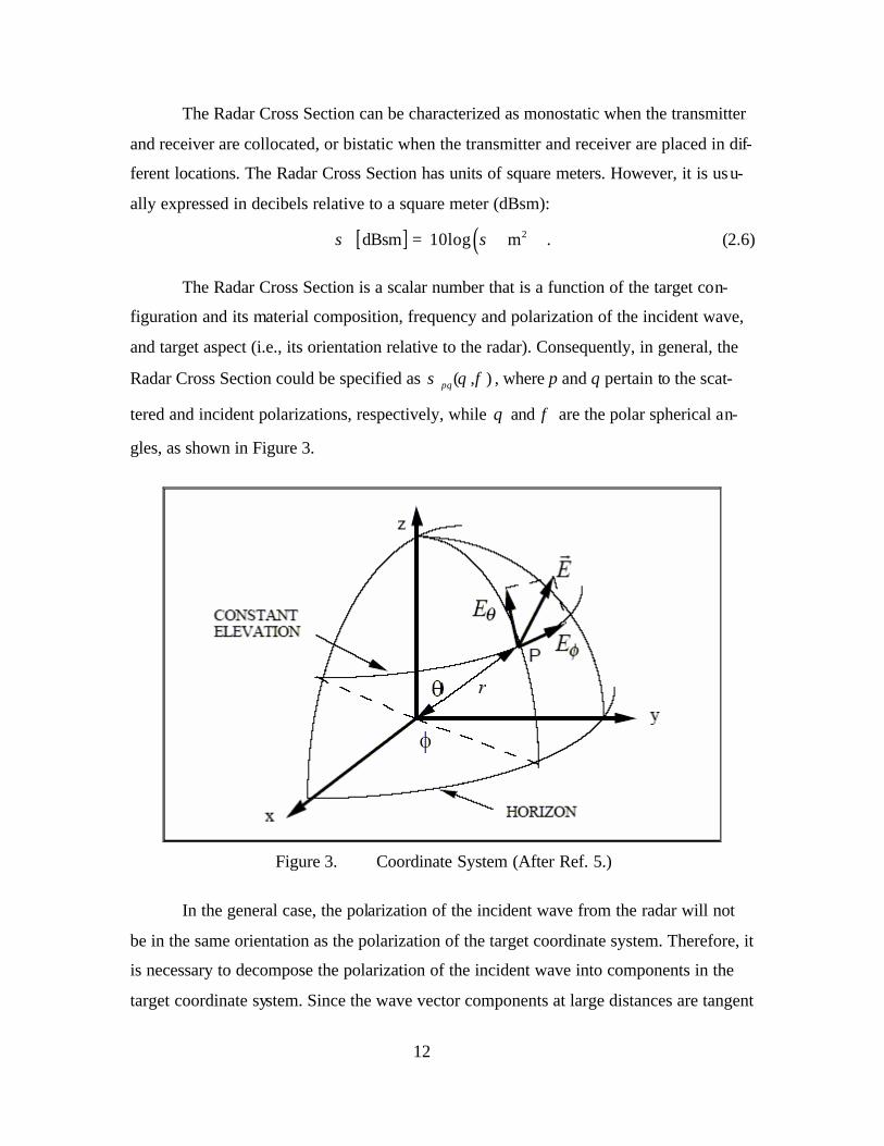
The Radar Cross Section is a scalar number that is a function of the target con-

figuration and its material composition, frequency and polarization of the incident wave,

and target aspect (i.e., its orientation relative to the radar). Consequently, in general, the

Radar Cross Section could be specified as ( , )pqσ θ φ , where p and q pertain to the scat-

tered and incident polarizations, respectively, while θ and φ are the polar spherical an-

gles, as shown in Figure 3.

Figure 3. Coordinate System (After Ref. 5.)

In the general case, the polarization of the incident wave from the radar will not

be in the same orientation as the polarization of the target coordinate system. Therefore, it

is necessary to decompose the polarization of the incident wave into components in the

target coordinate system. Since the wave vector components at large distances are tangent

13

to a sphere, two orthogonal components in terms of the variables θ and φ are sufficient

to represent the incident field in a spherical system centered at the target. Thus, in gen-

eral, it is possible to write the incident field as:

ˆ ˆi i iE E Eθ φθ φ= +

r (2.7)

where θ and φ are the unit vectors in the target coordinate system and the index i signi-

fies incident field (Ref. 2).

In addition, the polarization of the scattered field will not necessarily be the same

as the incident field, since most complex targets generate a cross–polarized scattering

component due to multiple diffractions and reflections. The scattering matrix reflects this,

and it can be used to specify the relationship between the polarization of the incident and

the scattered field:

s i

s i

SE S E

E S ESθφθ θθ θ

φ φθ φφφ

=

(2.8)

where the index s denotes the scattered field.

The pqS symbols represent the scattering parameters, with the index p specifying

the scattered field polarization and the index q specifying the incident field polarization.

The elements of the scattering matrix are complex quantities related to the RCS with the

following equation (Ref. 2):

24

pqpqS

R

σ

π= . (2.9)

It is possible to write this in terms of amplitude and phase as:

1/2

24

pqjpq

pq

eS

R

ψσ

π= (2.10)

where

( )( )

Imarctan

Repq

pqpq

σψ

σ

=

(2.11)

and ( )Re ⋅ and ( )Im ⋅ are the real and imaginary operators.

14

D. SCATTERING REGIONS

As mentioned in the previous paragraphs, the Radar Cross Section depends on the

frequency of the incident wave. There are three frequency regions in which the RCS of a

target is distinctly different. The regions are defined based on the size of the target in

terms of the incident wavelength. For a smooth target of length L, the definitions of the

three frequency regimes follow.

1. Low Frequency Region or Rayleigh Region 2

1Lπλ

<<

At these frequencies, the phase variation of the incident plane wave across the ex-

tent of the target is small. Thus, the induced current on the body of the target is approxi-

mately constant in amplitude and phase. The particular shape of the body is not impor-

tant. Generally, σ versus 2

Lπλ

is smooth and varies as 41/ λ (Ref. 2).

2. Resonance Region or Mie Region 2

1Lπλ

≈

For these frequencies, the phase variation of the current across the body of the

target is significant and all parts contribute to the scattering. Generally, σ versus 2

Lπλ

and will oscillate (Ref. 2).

3. High Frequency Region or Optical Region 2

1Lπλ

>>

For these frequencies, there are many cycles in the phase variation of the current

across the target body and, consequently, the scattered field will be very angle–

dependent. In this region, σ versus 2

Lπλ

is smooth and may be independent of λ (Ref.

2).

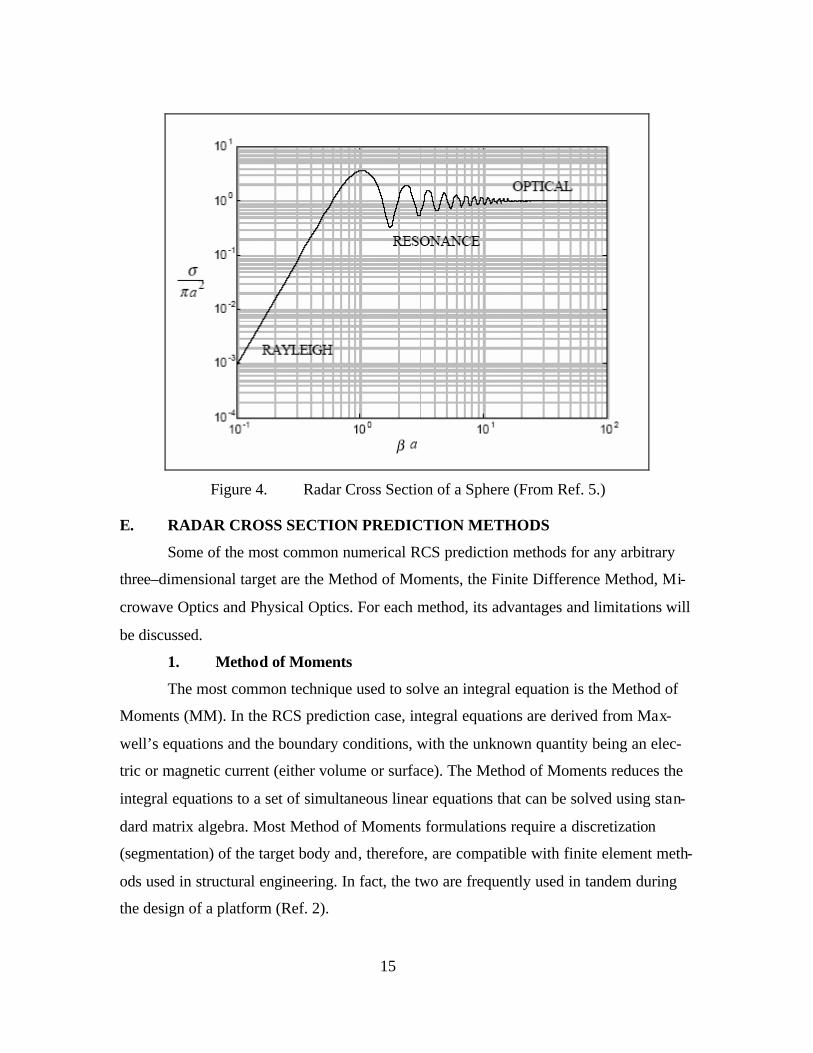
Figure 4 depicts the Radar Cross Section of a sphere with radius a , where β is

defined as 2β π λ= . The three scattering regions are clearly illustrated. When 0.5aβ < ,

the curve in the Rayleigh region is almost linear. However, above 0.5, in the resonance

region, the RCS oscillates. The oscillations die out as aβ takes higher values. Eventu-

ally, for 10aβ > , the value of the RCS is essentially constant and equal to 2aπ .

15

Figure 4. Radar Cross Section of a Sphere (From Ref. 5.)

E. RADAR CROSS SECTION PREDICTION METHODS

Some of the most common numerical RCS prediction methods for any arbitrary

three–dimensional target are the Method of Moments, the Finite Difference Method, Mi-

crowave Optics and Physical Optics. For each method, its advantages and limitations will

be discussed.

1. Method of Moments

The most common technique used to solve an integral equation is the Method of

Moments (MM). In the RCS prediction case, integral equations are derived from Max-

well’s equations and the boundary conditions, with the unknown quantity being an elec-

tric or magnetic current (either volume or surface). The Method of Moments reduces the

integral equations to a set of simultaneous linear equations that can be solved using stan-

dard matrix algebra. Most Method of Moments formulations require a discretization

(segmentation) of the target body and, therefore, are compatible with finite element meth-

ods used in structural engineering. In fact, the two are frequently used in tandem during

the design of a platform (Ref. 2).

16

Another advantage of the Method of Moments is that it provides a rigorous solu-

tion to the RCS prediction problem, yielding very accurate results. However, this method

tends to produce large matrices, resulting in high computational requirements and in-

creased run time. In addition, since current computer capabilities allow the modeling of

targets on the order of 10 to 20 wavelengths, the method is not practical for large targets

at high frequencies due to computer limitations (Refs. 1 and 3).

2. Finite Difference Methods

Finite Difference methods are used to approximate the differential operators in

Maxwell’s equations in either the time or frequency domain. Similar to the Method of

Moments, the target must be discretized. Maxwell’s equations and the boundary cond i-

tions are enforced on the surface of the target and at the boundaries of the discretization

cells. In the time domain, this method is used extensively in computing transient re-

sponses of targets to various waveforms. Since the solution is stepped in time throughout

the scattering body, the finite difference method does not require large matrices as does

the Method of Moments. Frequency domain data is obtained by Fourier–transforming the

time data.

This method also provides a rigorous solution to the RCS prediction problem.

However, since it calculates the fields in a computational grid around the target, the cal-

culation of the RCS of a target with a characteristic dimension of several orders of mag-

nitude of the wavelength would entail considerable amount of time to execute (Refs. 1

and 3).

3. Microwave Optics

Ray tracing methods that can be used to analyze electrically large targets of arbi-

trary shape are referred to as Microwave Optics. This term actually refers to a collection

of ray tracing techniques that can be used individually or in concert. The two most used

are the Geometrical Optics (GO) method and the Geometrical Theory of Diffraction

(GTD) method. The rules for ray tracing in a simple medium (i.e., linear, homogenous

and isotropic) are similar to reflection and refraction in optics. In addition, this method

takes into account diffracted rays, which originate from the scattering of the incident

wave at edges, corners and vertices. The formulae are derived on the basis of infinite fre-

17

quency ( 0)λ → , which implies an electrically large target. The major disadvantage of

this method is the bookkeeping required when tracking a large number of reflections and

diffractions for complex targets.

4. Physical Optics

The Physical Optics (PO) method estimates the surface current induced on an ar-

bitrary body by the incident radiation. On the portions of the body that are directly illu-

minated by the incident field, the induced current is simply proportional to the incident

magnetic field intensity. On the shadowed portion of the target, the current is set to zero.

The current is then used in the radiation integrals to compute the scattered field far from

the target (Ref. 2).

This method is a high frequency approximation that provides the best results for

electrically large targets as well as in the specular direction. Since it abruptly sets the cur-

rent to zero at the shadow boundary, the computed field values at wide angles and in the

shadow regions are inaccurate. Furthermore, surface waves, multiple reflections and edge

diffractions are not included (Refs. 1 and 3). However, the simplicity of the approach en-

sures low demands on computing resources and convenient run–times.

The POFACETS program utilizes the Physical Optics method to compute the sur-

face currents on the triangular facets that comprise the building blocks of a target model.

Then, the radiation integrals are used to compute the scattered field.

F. SUMMARY

This chapter discussed the importance of RCS, its role in the radar equation, and

its significance in the outcome of military engagements. It provides the formal definition

of RCS and discusses its behavior in the three scattering regions. Finally, the most com-

mon methods for RCS prediction are described. The next chapter discusses the mathe-

matical equations and the theory that pertains to these computations.

18


19

III. PHYSICAL OPTICS APPLIED TO TRIANGULAR FACET MODELS

This chapter contains the theoretical framework of the Physical Optics approxi-

mation method and the mathematical formulations used in the POFACETS program to

implement this method. Starting from the radiation integrals for an arbitrary object, the

scattered field formulas are derived for the case of a triangular facet. The Phys ical Optics

approximation is used to provide values for the surface currents on a facet and Taylor se-

ries are utilized to calculate the scattered field. In the process, all tools and fo rmulas used

in the calculations are defined and explained. Finally, the computational model is ex-

panded to implement the calculation of the scattered field from a collection of facets (i.e.,

an arbitrary target model).

A. RADIATION INTEGRALS FOR FAR ZONE SCATTERED FIELDS

The scattering from a triangular facet is a special case of the scattering from an

arbitrary body. Hence, the formula for the scattered field for a triangular facet will be de-

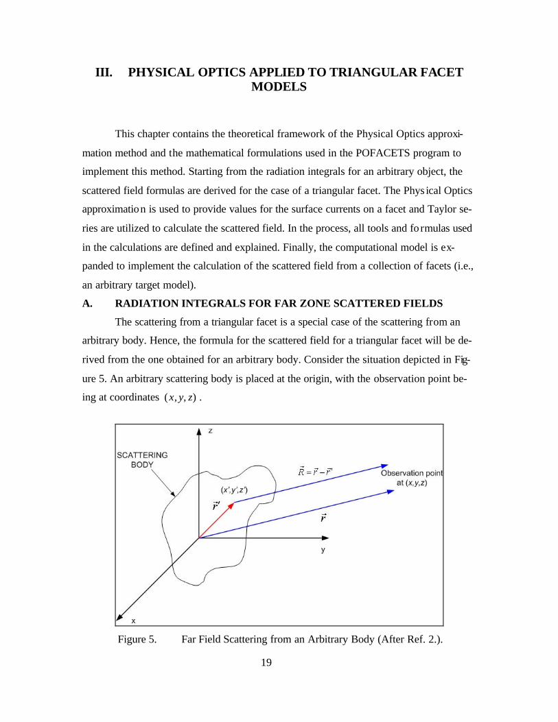
rived from the one obtained for an arbitrary body. Consider the situation depicted in Fig-

ure 5. An arbitrary scattering body is placed at the origin, with the observation point be-

ing at coordinates ( , , )x y z .

Figure 5. Far Field Scattering from an Arbitrary Body (After Ref. 2.).

20

For Radar Cross Section calculations, the observation point is considered to be in

the far zone of the target. Thus, the vectors Rr

and rr are approximately parallel.

The body is segmented into infinitely small source points of volume v′ located at

coordinates ( , , )x y z′ ′ ′ . The position vector to a source point is:

ˆ ˆ ˆr xx yy zz′ ′ ′ ′= + +r (3.1)

with ˆ ˆ ˆ, , x y z being the coordinate–axes unit vectors.

The unit vector in the direction of the observation point is:

ˆ ˆ ˆ ˆr xu y zwυ= + + (3.2)

where

sin cossin sincos

u

w

θ φυ θ φ

θ

===

(3.3)

with θ and φ being the spherical coordinates of the observation point.

Assuming that the magnetic volume current in the body is 0mJ =r

, the scattered

field from the body is given by the following equation:

ˆ ˆ( , , ) ( , , ) ( , , )4

jkr jkgos V

jkZE r E r E r e Je drθ φθ φ θ φ θ θ φ φ υ

π−− ′= + = ∫∫∫

r r (3.4)

where Jr

is the electric volume current, oZ is the intrinsic impedance of the space sur-

rounding the body, 2k π λ= (with λ being the wavelength) and g is defined as:

ˆg r r x u y z wυ′ ′ ′ ′= ⋅ = + +r . (3.5)

Notice that in Equation (3.4), the electric field has components only in the θ and φ di-

rection, so that the rE component in (3.4) is ignored (Ref. 2).

B. RADIATION INTEGRALS FOR A TRIANGULAR FACET

Consider a triangular facet with arbitrary orientation defined by the vertices 1, 2

and 3, as shown in Figure 6.

21

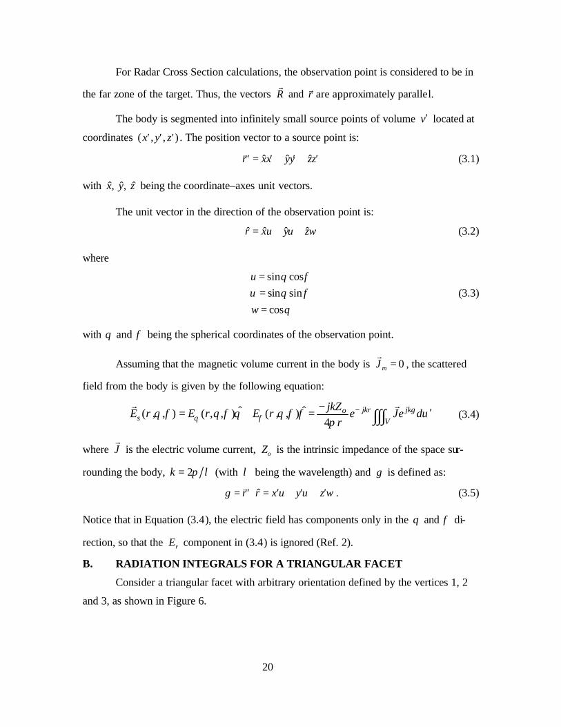
Figure 6. Arbitrary Oriented Facet (After Ref. 3.).

The integration point now is P , which is located at coordinates ,( , )p p px y z cor-

responding to the ( , , )x y z′ ′ ′ coordinates of the integration point for the arbitrary body ex-

amined in the previous section. Its position vector is

ˆ ˆ ˆp p p pr x x y y z z= + +r

. (3.6)

Since the triangular facet is a two–dimensional object, the volume integration in

Equation (3.4) becomes a surface integration. Similarly, there is only surface current

flowing on the triangular facet. Hence, Equation (3.4) becomes:

( , , )4

jkr jkgos s pA

jkZE r e J e ds

rθ φ

π−−

= ∫∫r r

(3.7)

where sJr

is the surface current, A the area of the triangular facet, pds the differential

surface area and g is defined as:

ˆp p p pg r r x u y z wυ= ⋅ = + +r

. (3.8)

Hence, the problem of evaluating the scattered field from a single facet has been

narrowed to two simpler problems: (1) the computation of the surface current sJr

flowing

on the facet by using the Physical Optics method, and (2) the computation of the integral

in Equation (3.7).

22

It is necessary to describe some of the tools to be used in the calculations before

addressing these two problems.

C. RADIATION INTEGRALS FOR A TRIANGULAR FACET

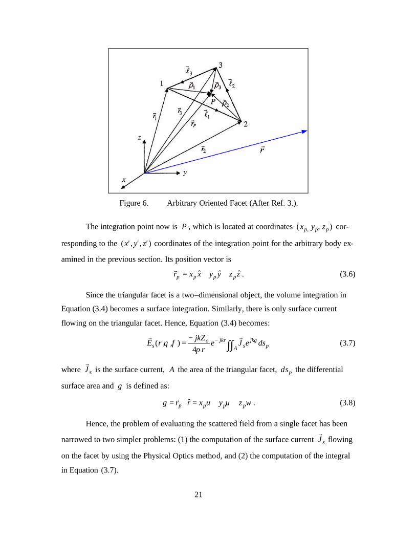
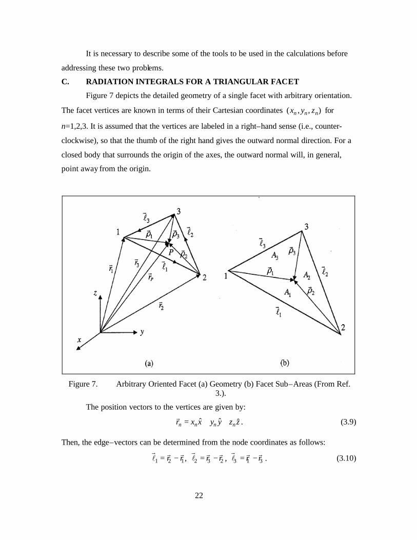
Figure 7 depicts the detailed geometry of a single facet with arbitrary orientation.

The facet vertices are known in terms of their Cartesian coordinates ( , , )n n nx y z for

n=1,2,3. It is assumed that the vertices are labeled in a right–hand sense (i.e., counter-

clockwise), so that the thumb of the right hand gives the outward normal direction. For a

closed body that surrounds the origin of the axes, the outward normal will, in general,

point away from the origin.

Figure 7. Arbitrary Oriented Facet (a) Geometry (b) Facet Sub–Areas (From Ref.

3.).

The position vectors to the vertices are given by:

ˆ ˆ ˆn n n nr x x y y z z= + +r

. (3.9)

Then, the edge–vectors can be determined from the node coordinates as follows:

1 2 1 2 3 2 3 1 3, , r r r r r r= − = − = −r r rr r r r r rl l l . (3.10)

23

The outward normal of the facets can then be obtained by taking the cross product of any

two edge–vectors in a right–hand sense. For example:

1 3

1 3

ˆ ˆ ˆ ˆx y zn n x n y n z×

= ≡ + +r rl lr rl l

. (3.11)

With this ordering of the vertices, the outward side of the facet is denoted as the

front face with the opposite side being the back face. If a plane wave is incident from an

angle ( , )i iθ φ , propagating towards the origin, then its propagation vector is:

ˆ ˆ ˆ ˆ ˆ( )i i i ik r xu y zwυ= − = − + + (3.12)

where ( , , )i i iu wυ are the direction cosines and r is the radial unit vector from the origin

to the source at ( , )i iθ φ . A front facet is illuminated when the following condition is satis-

fied:

ˆ ˆ 0ik n− ⋅ ≥ (3.13)

It is possible to compute the total area of the facet A from the cross product of the

two edge vectors:

1 312

A = ×r rl l . (3.14)

In order to simplify integration over the surface of the facets, normalized areas are

used. Specifically, sub–areas 1 2 3, ,A A A are defined, from which normalized area coordi-

nates are computed:

31 2, , AA A

A A Aζ ξ η= = = . (3.15)

Since 1 2 3A A A A+ + = , it is possible to write 1ζ ξ η+ + = , and hence, 1ζ ξ η= − − .

Then, the integration over the area of the facet can be written as (Ref. 3):

1 1

0 02pA

ds A d dη

ξ η−

=∫∫ ∫ ∫ . (3.16)

24

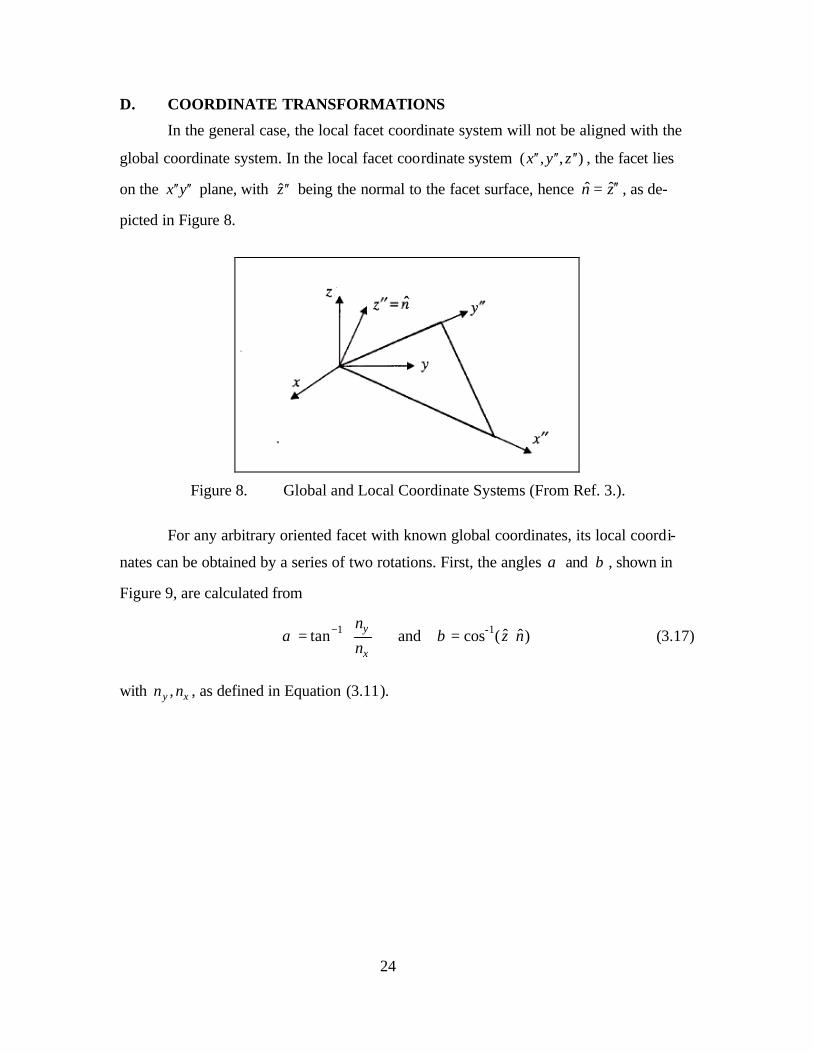
D. COORDINATE TRANSFORMATIONS

In the general case, the local facet coordinate system will not be aligned with the

global coordinate system. In the local facet coordinate system ( , , )x y z′′ ′′ ′′ , the facet lies

on the x y′′ ′′ plane, with z′′ being the normal to the facet surface, hence ˆ ˆn z′′= , as de-

picted in Figure 8.

Figure 8. Global and Local Coordinate Systems (From Ref. 3.).

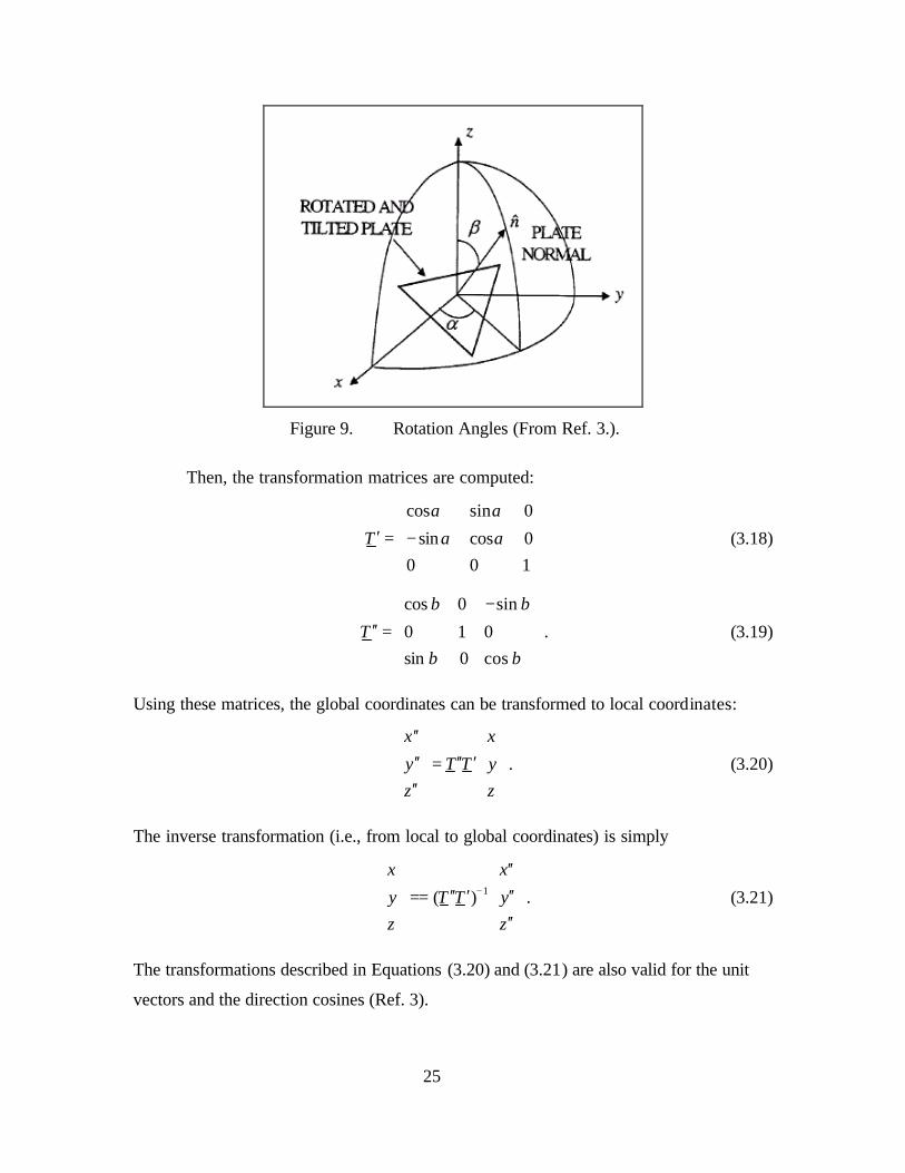
For any arbitrary oriented facet with known global coordinates, its local coordi-

nates can be obtained by a series of two rotations. First, the angles α and β , shown in

Figure 9, are calculated from

1 -1 ˆˆtan and cos ( )y

x

nz n

nα β−

= = ⋅

(3.17)

with ,y xn n , as defined in Equation (3.11).

25

Figure 9. Rotation Angles (From Ref. 3.).

Then, the transformation matrices are computed:

cos sin 0

sin cos 00 0 1

T

α α

α α ′ = −

(3.18)

cos 0 sin

0 1 0sin 0 cos

T

β β

β β

− ′′ =

. (3.19)

Using these matrices, the global coordinates can be transformed to local coordinates:

x x

y T T yz z

′′ ′′ ′′ ′=

′′

. (3.20)

The inverse transformation (i.e., from local to global coordinates) is simply

1( )

x x

y T T yz z

−

′′ ′′ ′ ′′==

′′

. (3.21)

The transformations described in Equations (3.20) and (3.21) are also valid for the unit

vectors and the direction cosines (Ref. 3).

26

E. PHYSICAL OPTICS SURFACE CURRENT COMPUTATION

According to the Physical Optics method, on the portions of the body that are di-

rectly illuminated by the incident field, the induced current is simply proportional to the

incident magnetic field intensity. On the shadowed portion of the target, the current is set

to zero. Hence:

ˆ2 for the illuminated facets

0 for the shadowed facets i

sn H

J ×

=

rr

(3.22)

where iHr

is the incident magnetic field intensity at the surface.

In general, the incident field is of the form

ˆ ˆ( ) ijk ri i iE E E eθ φθ φ −= +

r rir (3.23)

where ˆ ˆ , with 2i i ik kk kr k π λ= = − =r

. Since ˆ ˆpr r= for a point ( , , )p p px y z on the surface:

ˆˆ ˆ( ) i pjkr r

i i iE E E eθ φθ φ= +rir

. (3.24)

Then, the magnetic field intensity is:

ˆ1 ˆ ˆ( ) i pjkr ri i

i i io o

k EH E E e

Z Z φ θθ φ×

= = −ri

r rr. (3.25)

The physical optics approximation for the surface current flowing on the facet is:

2 ˆ ˆˆ2 ( ) jkh

s i i io

J n H E E eZ φ θθ φ= × = −

r r (3.26)

where h is defined as:

ˆp i p i p i p ih r r x u y z wυ= = + +r i . (3.27)

It is now possible to write Equation (3.26) as:

ˆ ˆ ˆ( ) jkhs x y zJ J x J y J z e= + +

r. (3.28)

However, in facet local coordinates, the surface current does not have a z′′ component,

since the facet lies on the x y′′ ′′ plane. Hence:

ˆ ˆ( ) jkhs x yJ J x J y e′′ ′′ ′′ ′′= +

r. (3.29)

The values of the surface current components are (Ref. 3):

27

sincos

cosiix

EEJ φθ

ο ο

φφθ⊥

′′ ′′ ′′ ′′′′ ′′= − Γ + Γ Ζ Ζ

P (3.30)

cossin

cosiiy

EEJ φθ

ο ο

φφθ⊥

′′ ′′ ′′ ′′′′ ′′= − Γ − Γ Ζ Ζ

P (3.31)

where ,i iE Eθ φ′′ ′′ are the components of the incident field in the local facet coordinates and

,θ φ′′ ′′ are the spherical polar angles of the local coordinates.

Various materials can be handled by the inclusion of and ⊥Γ ΓP , the transverse

magnetic (TM) and the transverse electric (TE) reflection coefficients, respectively.

These are defined as:

cos

2 coso

TMs o

ZR Z

θθ

′′−Γ = Γ =

′′+P (3.32)

2 cos

oTE

s o

ZR Zθ⊥

−Γ = Γ =

′′ + (3.33)

with sR being the surface resistivity of the facet material. When 0sR = , the surface is a

perfect electric conductor. As sR → ∞ , the surface becomes transparent ( )0Γ → .

F. SCATTERED FIELD COMPUTATION

To obtain the scattered field, simply replace Equation (3.29) in the radiation inte-

gral for the triangular facet, which was determined in Equation (3.7), so

( )ˆ ˆ( , , ) ( )4

jkr jk g hos x y pA

jkZE r e J x J y e ds

rθ φ

π− +− ′′ ′′ ′′ ′′= + ∫∫

r. (3.34)

In order to compute the scattered field, it is only necessary to evaluate the inte-

gral:

( )jk g hc pA

I e ds+= ∫∫ . (3.35)

However, it is not possible to obtain an exact closed form solution for this integral. Given

that the incident wavefront is assumed plane and that the incident field is known at the

facet vertices, the amplitude and phase at the interior integration points can

28

be found by interpolation. Then, the integrand can be expanded using Taylor series, and

each term integrated to give a closed form result. Usually, a small number of terms in the

Taylor series (on the order of 5) will give a sufficiently accurate approximation (Ref. 3).

Thus, using the notation of Ref. 6, the following equation is defined as:

( , )( , ) cjDc cA

I C e d dη ξη ξ η ξ= ∫∫ (3.36)

where

( , )c p q iC C C C Eοη ξ η ξ= + + ≡r

. (3.37)

For a unit amplitude plane wave:

1 0, 1i p q oE C C C= ⇒ = = =r

. (3.38)

Similarly,

( , )c p q oD D D Dη ξ η ξ= + + (3.39)

with

[ ][ ][ ]

1 3 1 3 1 3

2 3 2 3 2 3

3 3 3

( ) ( ) ( )

( ) ( ) ( )

p

q

o

D k x x u y y z z w

D k x x u y y z z w

D k x u y z w

υ

υ

υ

= − + − + −

= − + − + −

= + +

. (3.40)

Now the integral of Equation (3.35) is given by:

2( ) ( )

p qojD jDjD o o o

cp q p q q p p q

C C CI Ae e e

D D D D D D D D

= − −

− − . (3.41)

In order to avoid numerical errors that occur near the singularities (i.e., denomina-

tors near zero), the following special cases are considered separately:

Case 1: and p t q tD L D L< ≥

0

( )2( , )

! 1

oq

njDjDp o

c o qq n

jD CAeI e C G n D

jD n n

∞

=

= − + − +

∑ (3.42)

Case 2: and p t q tD L D L< <

0 0

( ) ( )2

( 2)!o

n mo p qjD

cn m

C jD jDI Ae

m n

∞ ∞

= ==

+ +∑ ∑ (3.43)

29

Case 3: and p t q tD L D L≥ <

0

( )2 ( 1, )

! 1po

njD qjD o

c pn

jD CI Ae e G n D

n n

∞

== + −

+∑ (3.44)

Case 4: and p t q tD L D L≥ ≥

0

( )2( , )

! 1

pon jDjD

p q oc o q

q n

jD jD e CAeI C G n D

jD n n

∞

=

− = − + +

∑ (3.45)

where tL is the length of the Taylor series region. The function G is defined by

1

0

( , ) n j sG n s e dsγγ = ∫ (3.46)

and is evaluated with the use of the following recursive relationship:

( 1, )

( , ) , 1je nG n

G n nj

γ γγ

γ− −

= ≥ (3.47)

with

1

(0, )j

je

Ge

γ

γγ−

= . (3.48)

G. DIFFUSE FIELD COMPUTATION

Thus far, the discussion assumes that the facets are completely smooth. In reality,

of course, targets rarely have perfectly smooth surfaces, due to irregularities or material

and manufacturing imperfections. Surface roughness introduces path differences relative

to the smooth surface. Consequently, it is essential to consider a scattering component

due to these imperfections in the RCS computations.

Since the various imperfections in manufacturing and assembly processes of a

target tend to behave in a random fashion, the quantities chosen to represent these pa-

rameters can be modeled as random variables. The scattered field and the RCS are func-

tions of these random variables. The effect of the random errors on the resulting RCS pat-

tern is to subtract energy from the specular reflection, converting it to random scattering,

that is nearly equally distributed in all directions, which is called diffuse scattering (Ref.

2).

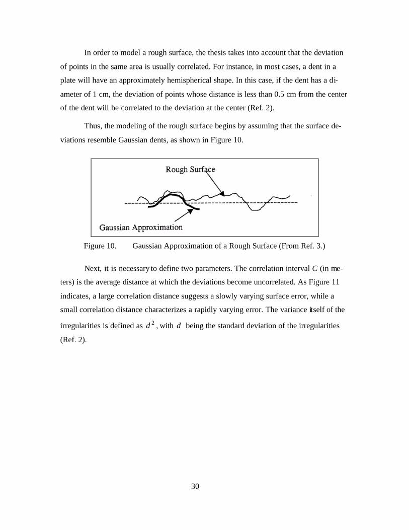
30

In order to model a rough surface, the thesis takes into account that the deviation

of points in the same area is usually correlated. For instance, in most cases, a dent in a

plate will have an approximately hemispherical shape. In this case, if the dent has a di-

ameter of 1 cm, the deviation of points whose distance is less than 0.5 cm from the center

of the dent will be correlated to the deviation at the center (Ref. 2).

Thus, the modeling of the rough surface begins by assuming that the surface de-

viations resemble Gaussian dents, as shown in Figure 10.

Figure 10. Gaussian Approximation of a Rough Surface (From Ref. 3.)

Next, it is necessary to define two parameters. The correlation interval C (in me-

ters) is the average distance at which the deviations become uncorrelated. As Figure 11

indicates, a large correlation distance suggests a slowly varying surface error, while a

small correlation distance characterizes a rapidly varying error. The variance itself of the

irregularities is defined as 2δ , with δ being the standard deviation of the irregularities

(Ref. 2).

31

Figure 11. (a) Large Correlation Distance, (b) Small Correlation Distance (From Ref.

3.)

The POFACETS program allows the user to select the correlation distance and

standard deviation. The average value of the RCS of a facet is approximately (Ref. 7):

2 2

2 2 2 2 2 2 24 2

2 2

4 4 sincos expk

aveA k C C

eA

δπ π δ π θσ θ

λ λ−

′′′′≈ −

(3.49)

with A being the area of the facet and θ ′′ the same as previously defined.

This value is simply added to the specular term, which is calculated using Equa-

tion (3.34).

H. TOTAL FIELD FROM A TARGET

Thus far, the discussion has involved the calculation of the scattered field from a

single facet. A large target is approximated by a model consisting of many triangular fac-

ets. Superposition is used to calculate the scattered field from the target. First, the scat-

tered field is computed for each facet. Then, the scattered field from each facet is vector–

summed to produce the total field in the observation direction. Once the scattered field is

known, the RCS in that direction is computed. This is repeated for all the observation di-

rections selected by the user. The entire process, including model generation and data

presentation has been programmed in the software package POFACETS.

Specifically, the following steps, diagramed in Figure 12, take place in the RCS

computation process:

32

1. The parameters of the RCS computation, including frequency, Taylor se-ries parameters, surface roughness parameters, angle of incidence (for bistatic RCS case), angles of observation, incident field polarization and model name are selected by the user.

2. The program reads the model characteristics (coordinates of facets, facet description and surface resistivity).

3. Initial computations are executed to obtain certain facet characteristics, in-cluding facet area, normal vector and rotation angles, using Equations (3.11), (3.14) and (3.17), respectively.

4. For each facet, its illumination condition is assessed, using Equation (3.13). If the facet is not illuminated, all scattered and diffuse components are set to zero and the program proceeds to the next facet. If the facet is il-luminated, the following steps are performed.

• The incident field, the angle of incidence (for the bistatic RCS case) and the observation angle are transformed to the local coor-dinate system of the facet, using the transformation described in Equation (3.20).

• The Physical Optics Current is computed from the incident mag-netic field, using Equations (3.30) and (3.31).

• The scattered field is computed in local facet coordinates using the radiation integral, via Equations (3.34) and (3.41) to (3.45).

• The diffuse component is computed using Equation (3.49).

• The scattered field is transformed back to global coordinates, using Equation (3.21).

• The scattered field components from each facet are superimposed (vector added) to obtain the total scattered field in the observation direction.

5. The diffuse and scattered RCS are computed from the total fields.

6. Steps 4 to 5 are repeated for each observation angle.

7. Selected graphical plots of RCS versus observation angle are displayed.

Notice that in the bistatic RCS calculation, the incidence angle is fixed. As a re-

sult, it is not necessary to compute the surface currents for each observation angle, con-

trary to what happens in the monostatic case, where the inc idence angle is the same as the

observation angle.

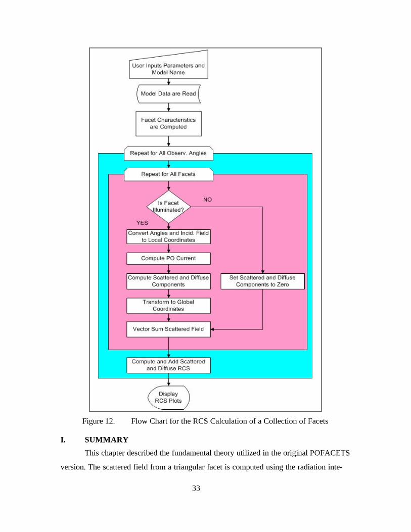
33

Figure 12. Flow Chart for the RCS Calculation of a Collection of Facets

I. SUMMARY

This chapter described the fundamental theory utilized in the original POFACETS

version. The scattered field from a triangular facet is computed using the radiation inte-

34

grals. The Physical Optics method is used to calculate the surface currents on each facet

and the scattered field from all facets of a model is vector summed to produce the RCS

value for given angles of incidence and observation. The next chapter presents the new

functionalities and improvements incorporated in the POFACETS program as a result of

this thesis.

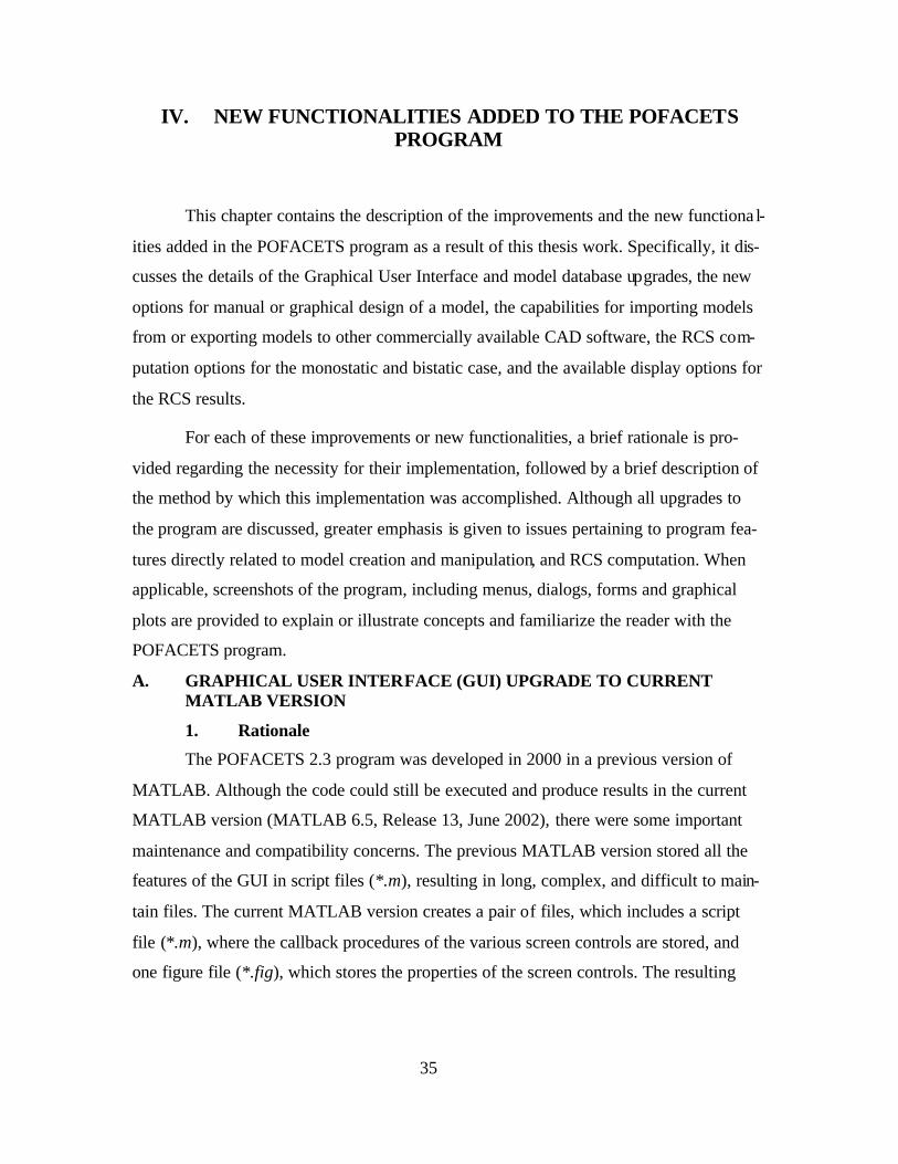
35

IV. NEW FUNCTIONALITIES ADDED TO THE POFACETS PROGRAM

This chapter contains the description of the improvements and the new functiona l-

ities added in the POFACETS program as a result of this thesis work. Specifically, it dis-

cusses the details of the Graphical User Interface and model database upgrades, the new

options for manual or graphical design of a model, the capabilities for importing models

from or exporting models to other commercially available CAD software, the RCS com-

putation options for the monostatic and bistatic case, and the available display options for

the RCS results.

For each of these improvements or new functionalities, a brief rationale is pro-

vided regarding the necessity for their implementation, followed by a brief description of

the method by which this implementation was accomplished. Although all upgrades to

the program are discussed, greater emphasis is given to issues pertaining to program fea-

tures directly related to model creation and manipulation, and RCS computation. When

applicable, screenshots of the program, including menus, dialogs, forms and graphical

plots are provided to explain or illustrate concepts and familiarize the reader with the

POFACETS program.

A. GRAPHICAL USER INTERFACE (GUI) UPGRADE TO CURRENT MATLAB VERSION

1. Rationale

The POFACETS 2.3 program was developed in 2000 in a previous version of

MATLAB. Although the code could still be executed and produce results in the current

MATLAB version (MATLAB 6.5, Release 13, June 2002), there were some important

maintenance and compatibility concerns. The previous MATLAB version stored all the

features of the GUI in script files (*.m), resulting in long, complex, and difficult to main-

tain files. The current MATLAB version creates a pair of files, which includes a script

file (*.m), where the callback procedures of the various screen controls are stored, and

one figure file (*.fig), which stores the properties of the screen controls. The resulting

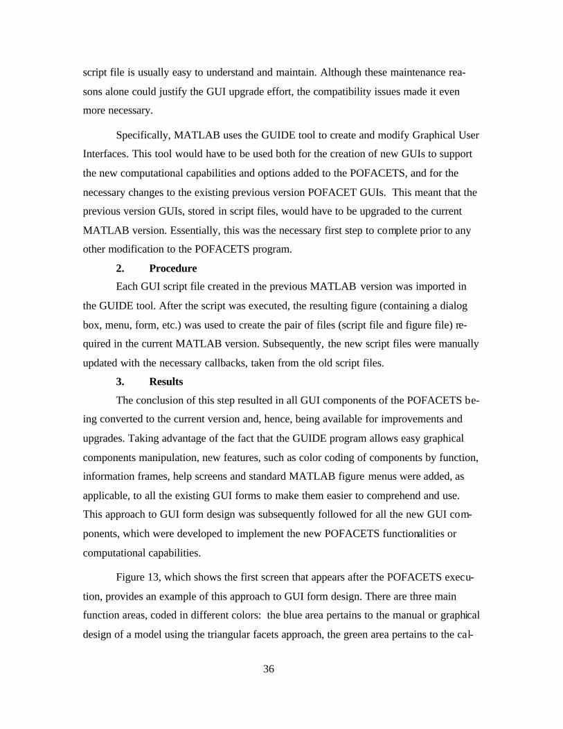
36

script file is usually easy to understand and maintain. Although these maintenance rea-

sons alone could justify the GUI upgrade effort, the compatibility issues made it even

more necessary.

Specifically, MATLAB uses the GUIDE tool to create and modify Graphical User

Interfaces. This tool would have to be used both for the creation of new GUIs to support

the new computational capabilities and options added to the POFACETS, and for the

necessary changes to the existing previous version POFACET GUIs. This meant that the

previous version GUIs, stored in script files, would have to be upgraded to the current

MATLAB version. Essentially, this was the necessary first step to complete prior to any

other modification to the POFACETS program.

2. Procedure

Each GUI script file created in the previous MATLAB version was imported in

the GUIDE tool. After the script was executed, the resulting figure (containing a dialog

box, menu, form, etc.) was used to create the pair of files (script file and figure file) re-

quired in the current MATLAB version. Subsequently, the new script files were manually

updated with the necessary callbacks, taken from the old script files.

3. Results

The conclusion of this step resulted in all GUI components of the POFACETS be-

ing converted to the current version and, hence, being available for improvements and

upgrades. Taking advantage of the fact that the GUIDE program allows easy graphical

components manipulation, new features, such as color coding of components by function,

information frames, help screens and standard MATLAB figure menus were added, as

applicable, to all the existing GUI forms to make them easier to comprehend and use.

This approach to GUI form design was subsequently followed for all the new GUI com-

ponents, which were developed to implement the new POFACETS functionalities or

computational capabilities.

Figure 13, which shows the first screen that appears after the POFACETS execu-

tion, provides an example of this approach to GUI form design. There are three main

function areas, coded in different colors: the blue area pertains to the manual or graphical

design of a model using the triangular facets approach, the green area pertains to the cal-

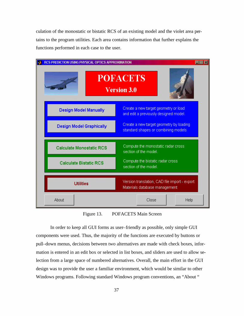
37

culation of the monostatic or bistatic RCS of an existing model and the violet area per-

tains to the program utilities. Each area contains information that further explains the

functions performed in each case to the user.

Figure 13. POFACETS Main Screen

In order to keep all GUI forms as user–friendly as possible, only simple GUI

components were used. Thus, the majority of the functions are executed by buttons or

pull–down menus, decisions between two alternatives are made with check boxes, infor-

mation is entered in an edit box or selected in list boxes, and sliders are used to allow se-

lection from a large space of numbered alternatives. Overall, the main effort in the GUI

design was to provide the user a familiar environment, which would be similar to other

Windows programs. Following standard Windows program conventions, an “About “

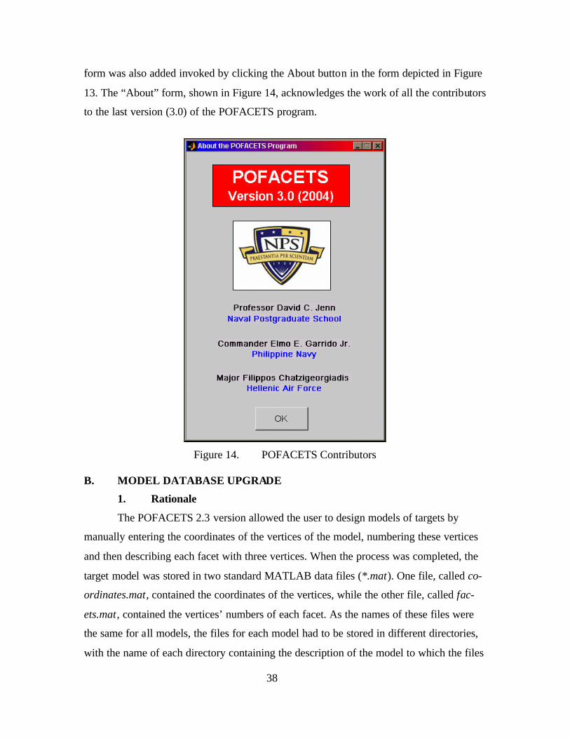
38

form was also added invoked by clicking the About button in the form depicted in Figure

13. The “About” form, shown in Figure 14, acknowledges the work of all the contributors

to the last version (3.0) of the POFACETS program.

Figure 14. POFACETS Contributors

B. MODEL DATABASE UPGRADE

1. Rationale

The POFACETS 2.3 version allowed the user to design models of targets by

manually entering the coordinates of the vertices of the model, numbering these vertices

and then describing each facet with three vertices. When the process was completed, the

target model was stored in two standard MATLAB data files (*.mat). One file, called co-

ordinates.mat, contained the coordinates of the vertices, while the other file, called fac-

ets.mat, contained the vertices’ numbers of each facet. As the names of these files were

the same for all models, the files for each model had to be stored in different directories,

with the name of each directory containing the description of the model to which the files

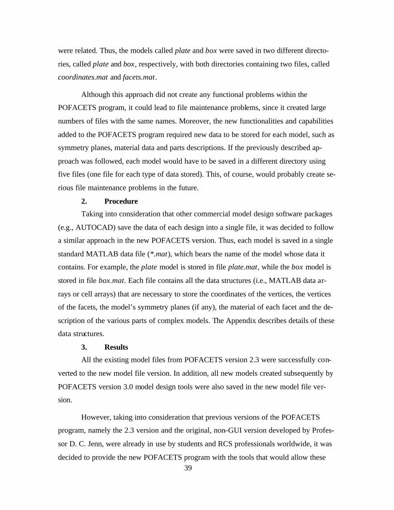
39

were related. Thus, the models called plate and box were saved in two different directo-

ries, called plate and box, respectively, with both directories containing two files, called

coordinates.mat and facets.mat.

Although this approach did not create any functional problems within the

POFACETS program, it could lead to file maintenance problems, since it created large

numbers of files with the same names. Moreover, the new functionalities and capabilities

added to the POFACETS program required new data to be stored for each model, such as

symmetry planes, material data and parts descriptions. If the previously described ap-

proach was followed, each model would have to be saved in a different directory using

five files (one file for each type of data stored). This, of course, would probably create se-

rious file maintenance problems in the future.

2. Procedure

Taking into consideration that other commercial model design software packages

(e.g., AUTOCAD) save the data of each design into a single file, it was decided to follow

a similar approach in the new POFACETS version. Thus, each model is saved in a single

standard MATLAB data file (*.mat), which bears the name of the model whose data it

contains. For example, the plate model is stored in file plate.mat, while the box model is

stored in file box.mat. Each file contains all the data structures (i.e., MATLAB data ar-

rays or cell arrays) that are necessary to store the coordinates of the vertices, the vertices

of the facets, the model’s symmetry planes (if any), the material of each facet and the de-

scription of the various parts of complex models. The Appendix describes details of these

data structures.

3. Results

All the existing model files from POFACETS version 2.3 were successfully con-

verted to the new model file version. In addition, all new models created subsequently by

POFACETS version 3.0 model design tools were also saved in the new model file ver-

sion.

However, taking into consideration that previous versions of the POFACETS

program, namely the 2.3 version and the original, non–GUI version developed by Profes-

sor D. C. Jenn, were already in use by students and RCS professionals worldwide, it was

decided to provide the new POFACETS program with the tools that would allow these

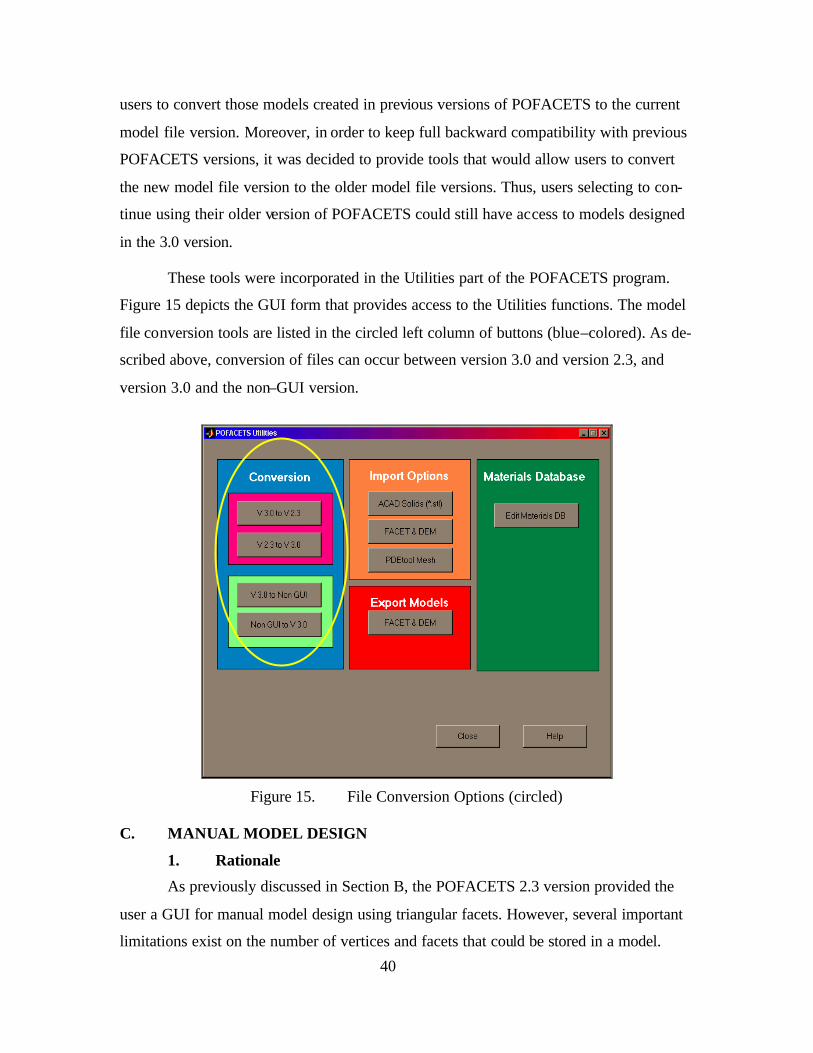
40

users to convert those models created in previous versions of POFACETS to the current

model file version. Moreover, in order to keep full backward compatibility with previous

POFACETS versions, it was decided to provide tools that would allow users to convert

the new model file version to the older model file versions. Thus, users selecting to con-

tinue using their older version of POFACETS could still have access to models designed

in the 3.0 version.

These tools were incorporated in the Utilities part of the POFACETS program.

Figure 15 depicts the GUI form that provides access to the Utilities functions. The model

file conversion tools are listed in the circled left column of buttons (blue–colored). As de-

scribed above, conversion of files can occur between version 3.0 and version 2.3, and

version 3.0 and the non–GUI version.

Figure 15. File Conversion Options (circled)

C. MANUAL MODEL DESIGN

1. Rationale

As previously discussed in Section B, the POFACETS 2.3 version provided the

user a GUI for manual model design using triangular facets. However, several important

limitations exist on the number of vertices and facets that could be stored in a model.

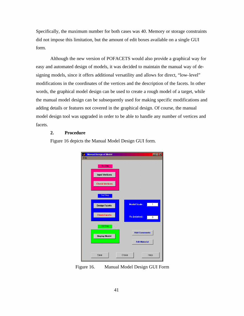
41

Specifically, the maximum number for both cases was 40. Memory or storage constraints

did not impose this limitation, but the amount of edit boxes available on a single GUI

form.

Although the new version of POFACETS would also provide a graphical way for

easy and automated design of models, it was decided to maintain the manual way of de-

signing models, since it offers additional versatility and allows for direct, “low–level”

modifications in the coordinates of the vertices and the description of the facets. In other

words, the graphical model design can be used to create a rough model of a target, while

the manual model design can be subsequently used for making specific modifications and

adding details or features not covered in the graphical design. Of course, the manual

model design tool was upgraded in order to be able to handle any number of vertices and

facets.

2. Procedure

Figure 16 depicts the Manual Model Design GUI form.

Figure 16. Manual Model Design GUI Form

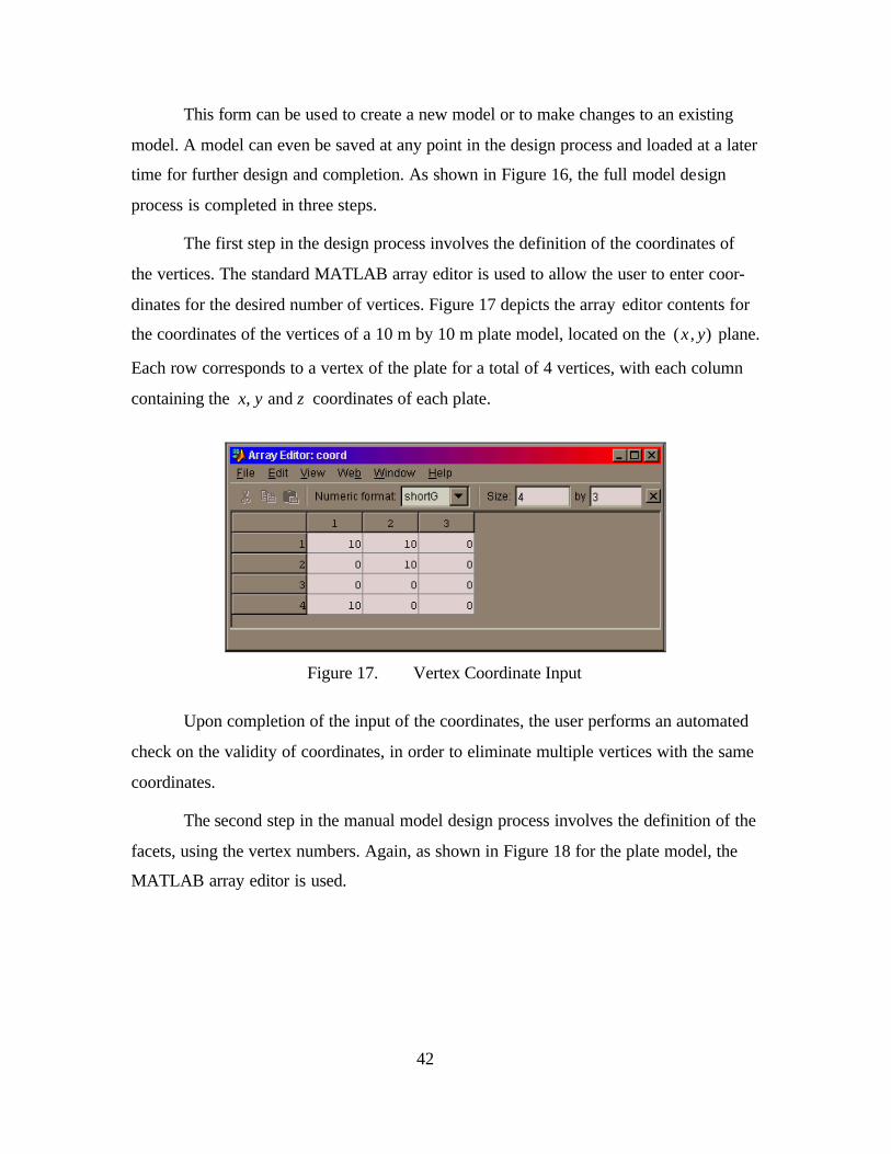
42

This form can be used to create a new model or to make changes to an existing

model. A model can even be saved at any point in the design process and loaded at a later

time for further design and completion. As shown in Figure 16, the full model design

process is completed in three steps.

The first step in the design process involves the definition of the coordinates of

the vertices. The standard MATLAB array editor is used to allow the user to enter coor-

dinates for the desired number of vertices. Figure 17 depicts the array editor contents for

the coordinates of the vertices of a 10 m by 10 m plate model, located on the ( , )x y plane.

Each row corresponds to a vertex of the plate for a total of 4 vertices, with each column

containing the , and x y z coordinates of each plate.

Figure 17. Vertex Coordinate Input

Upon completion of the input of the coordinates, the user performs an automated

check on the validity of coordinates, in order to eliminate multiple vertices with the same

coordinates.

The second step in the manual model design process involves the definition of the

facets, using the vertex numbers. Again, as shown in Figure 18 for the plate model, the

MATLAB array editor is used.

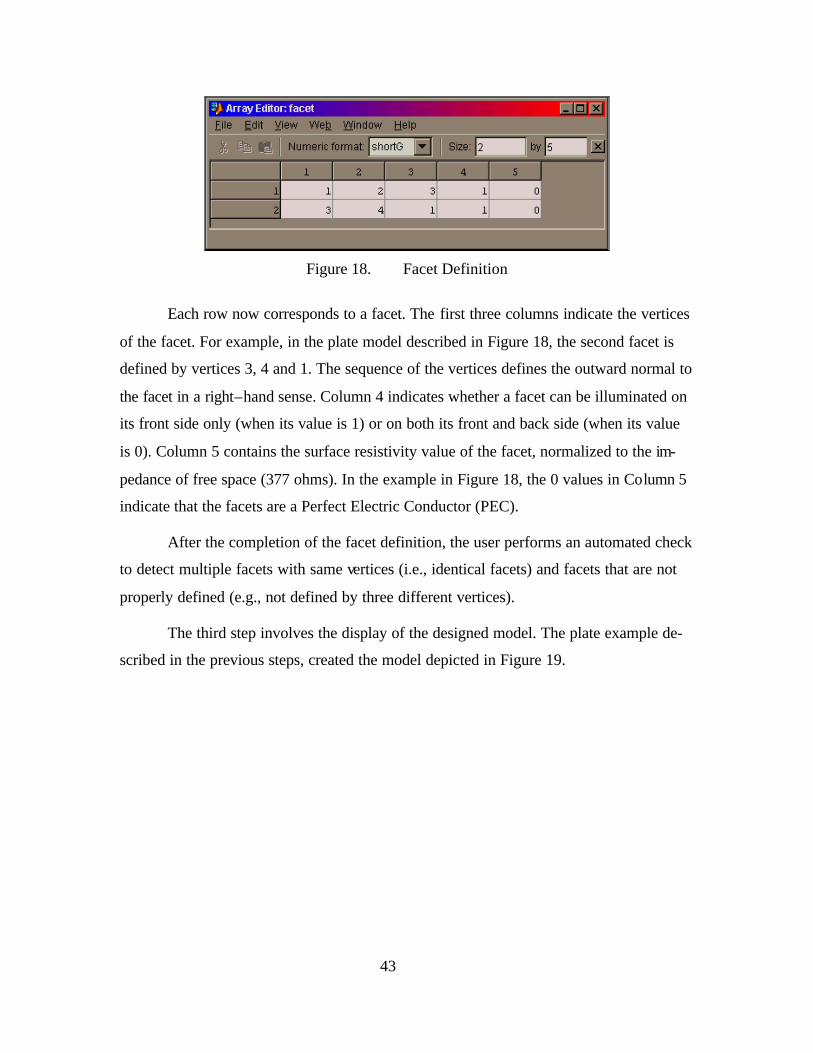
43

Figure 18. Facet Definition

Each row now corresponds to a facet. The first three columns indicate the vertices

of the facet. For example, in the plate model described in Figure 18, the second facet is

defined by vertices 3, 4 and 1. The sequence of the vertices defines the outward normal to

the facet in a right–hand sense. Column 4 indicates whether a facet can be illuminated on

its front side only (when its value is 1) or on both its front and back side (when its value

is 0). Column 5 contains the surface resistivity value of the facet, normalized to the im-

pedance of free space (377 ohms). In the example in Figure 18, the 0 values in Column 5

indicate that the facets are a Perfect Electric Conductor (PEC).

After the completion of the facet definition, the user performs an automated check

to detect multiple facets with same vertices (i.e., identical facets) and facets that are not

properly defined (e.g., not defined by three different vertices).

The third step involves the display of the designed model. The plate example de-

scribed in the previous steps, created the model depicted in Figure 19.

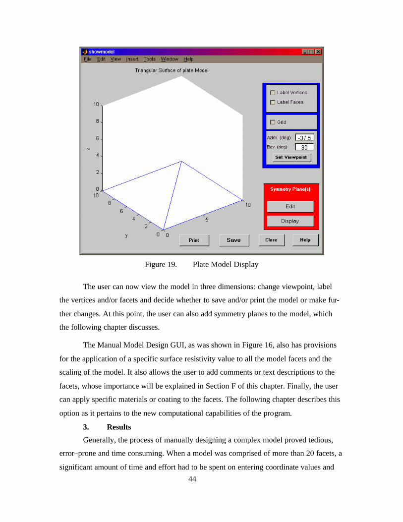
44

Figure 19. Plate Model Display

The user can now view the model in three dimensions: change viewpoint, label

the vertices and/or facets and decide whether to save and/or print the model or make fur-

ther changes. At this point, the user can also add symmetry planes to the model, which

the following chapter discusses.

The Manual Model Design GUI, as was shown in Figure 16, also has provisions

for the application of a specific surface resistivity value to all the model facets and the

scaling of the model. It also allows the user to add comments or text descriptions to the

facets, whose importance will be explained in Section F of this chapter. Finally, the user

can apply specific materials or coating to the facets. The following chapter describes this

option as it pertains to the new computational capabilities of the program.

3. Results

Generally, the process of manually designing a complex model proved tedious,

error–prone and time consuming. When a model was comprised of more than 20 facets, a

significant amount of time and effort had to be spent on entering coordinate values and

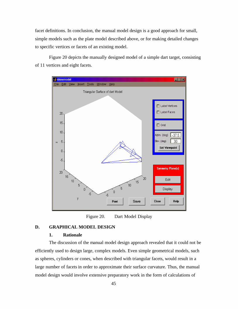
45

facet definitions. In conclusion, the manual model design is a good approach for small,

simple models such as the plate model described above, or for making detailed changes

to specific vertices or facets of an existing model.

Figure 20 depicts the manually designed model of a simple dart target, consisting

of 11 vertices and eight facets.

Figure 20. Dart Model Display

D. GRAPHICAL MODEL DESIGN

1. Rationale

The discussion of the manual model design approach revealed that it could not be

efficiently used to design large, complex models. Even simple geometrical models, such

as spheres, cylinders or cones, when described with triangular facets, would result in a

large number of facets in order to approximate their surface curvature. Thus, the manual

model design would involve extensive preparatory work in the form of calculations of

46

coordinates and time–consuming work to enter the coordinates to the program. Therefore,

a graphical, automated approach to model design was necessary to produce complex

models with minimum user workload.

2. Procedure

Since all standard geometrical shapes can be described with mathematical equa-

tions, many of which are implemented by standard MATLAB functions, the whole proc-

ess of model design could be easily automated by using these equations to find the values

of vertex coordinates. Once the coordinates are derived, the right–hand facet definition

approach can be used to produce the facet arrays

Figure 21 depicts the Graphical Model Design GUI form, which displays a model

of a cylinder.

Figure 21. Graphical Model Design GUI Form

This form can be used to create a new model or to make changes to an existing

model. As shown in Figure 21, there are provisions for the automatic model design of the

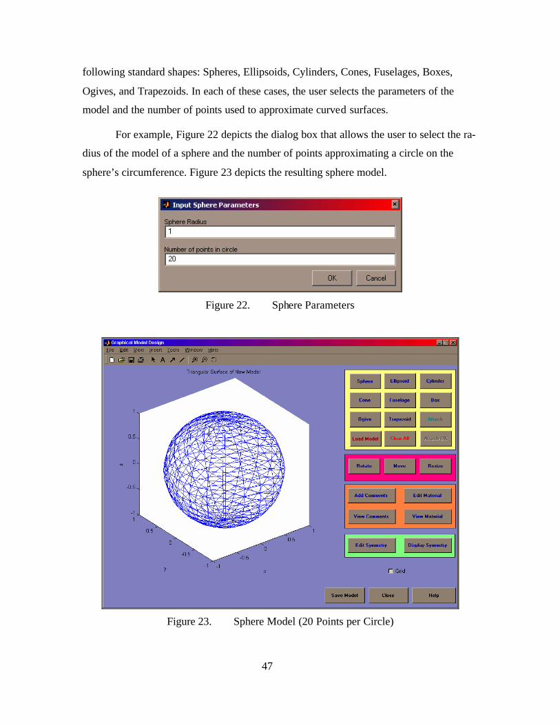
47

following standard shapes: Spheres, Ellipsoids, Cylinders, Cones, Fuselages, Boxes,

Ogives, and Trapezoids. In each of these cases, the user selects the parameters of the

model and the number of points used to approximate curved surfaces.

For example, Figure 22 depicts the dialog box that allows the user to select the ra-

dius of the model of a sphere and the number of points approximating a circle on the

sphere’s circumference. Figure 23 depicts the resulting sphere model.

Figure 22. Sphere Parameters

Figure 23. Sphere Model (20 Points per Circle)

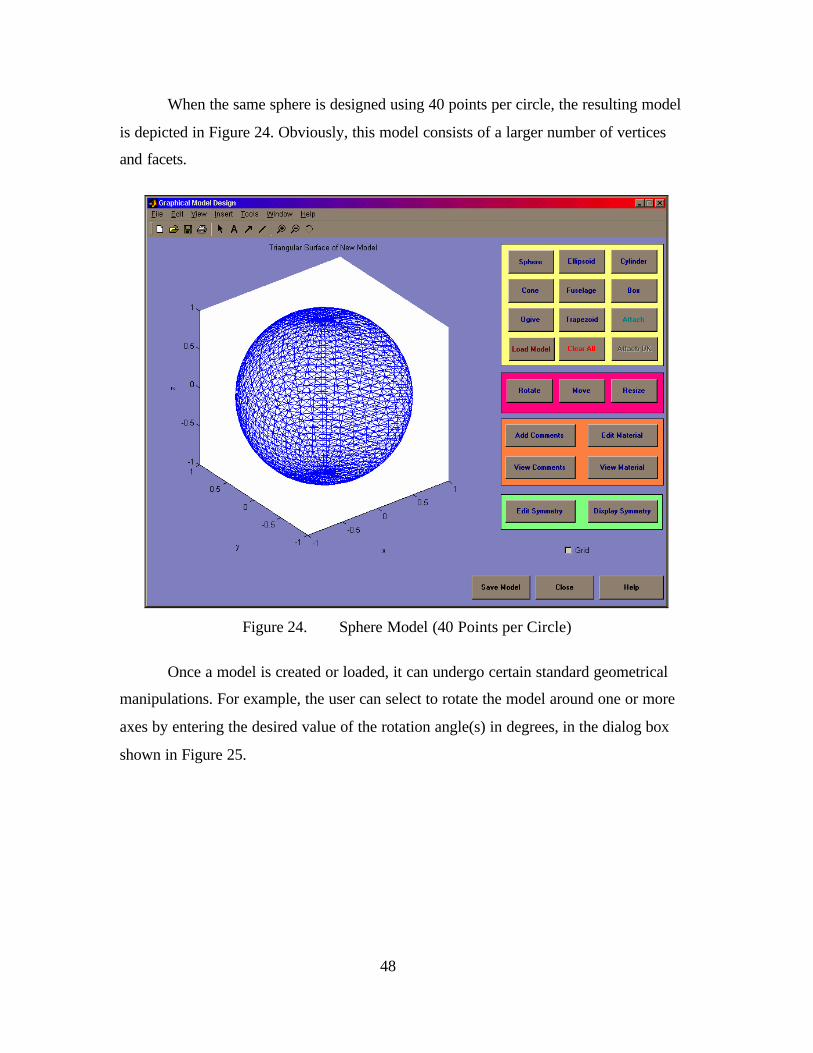
48

When the same sphere is designed using 40 points per circle, the resulting model

is depicted in Figure 24. Obviously, this model consists of a larger number of vertices

and facets.

Figure 24. Sphere Model (40 Points per Circle)

Once a model is created or loaded, it can undergo certain standard geometrical

manipulations. For example, the user can select to rotate the model around one or more

axes by entering the desired value of the rotation angle(s) in degrees, in the dialog box

shown in Figure 25.

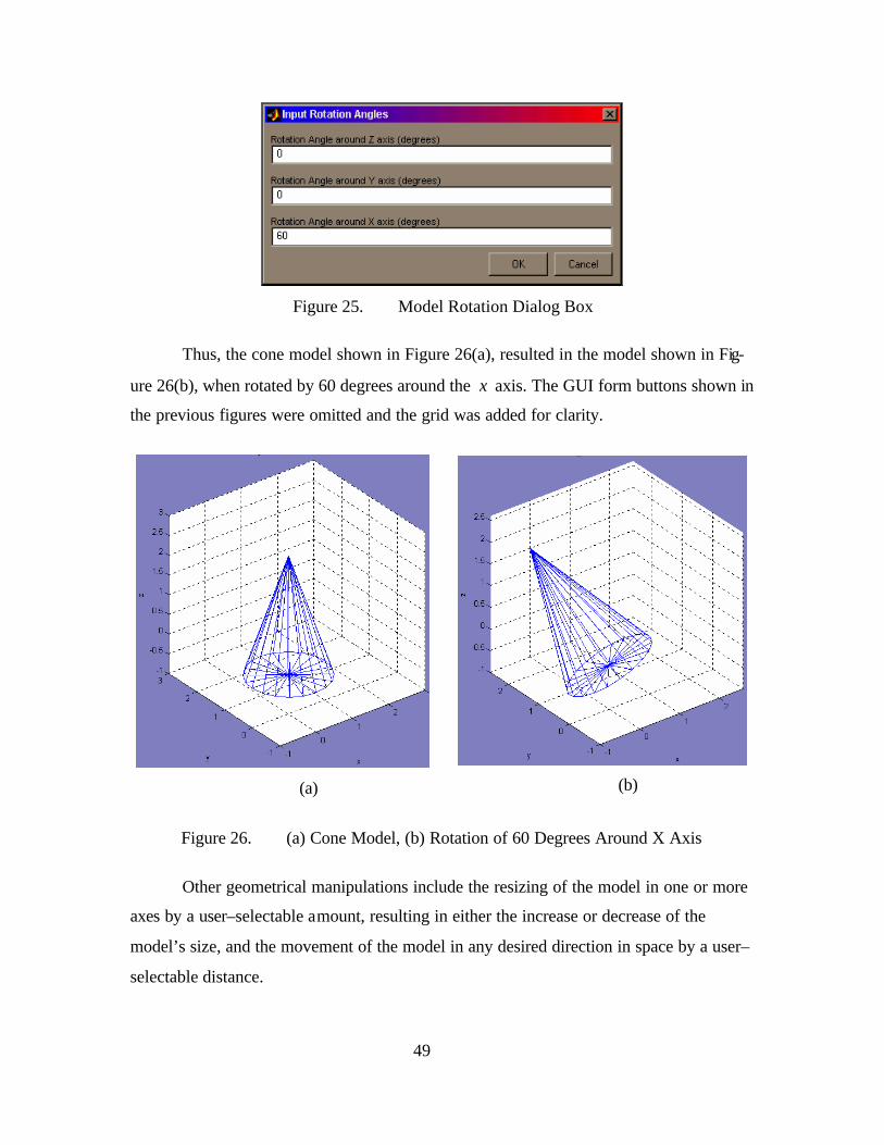
49

Figure 25. Model Rotation Dialog Box

Thus, the cone model shown in Figure 26(a), resulted in the model shown in Fig-

ure 26(b), when rotated by 60 degrees around the x axis. The GUI form buttons shown in

the previous figures were omitted and the grid was added for clarity.

(a)

(b)

Figure 26. (a) Cone Model, (b) Rotation of 60 Degrees Around X Axis

Other geometrical manipulations include the resizing of the model in one or more

axes by a user–selectable amount, resulting in either the increase or decrease of the

model’s size, and the movement of the model in any desired direction in space by a user–

selectable distance.

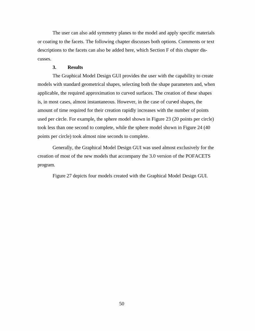
50

The user can also add symmetry planes to the model and apply specific materials

or coating to the facets. The following chapter discusses both options. Comments or text

descriptions to the facets can also be added here, which Section F of this chapter dis-

cusses.

3. Results

The Graphical Model Design GUI provides the user with the capability to create

models with standard geometrical shapes, selecting both the shape parameters and, when

applicable, the required approximation to curved surfaces. The creation of these shapes

is, in most cases, almost instantaneous. However, in the case of curved shapes, the

amount of time required for their creation rapidly increases with the number of points

used per circle. For example, the sphere model shown in Figure 23 (20 points per circle)

took less than one second to complete, while the sphere model shown in Figure 24 (40

points per circle) took almost nine seconds to complete.

Generally, the Graphical Model Design GUI was used almost exclusively for the

creation of most of the new models that accompany the 3.0 version of the POFACETS

program.

Figure 27 depicts four models created with the Graphical Model Design GUI.

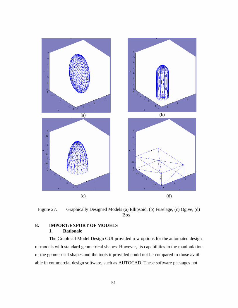
51

(a)

(b)

(c)

(d)

Figure 27. Graphically Designed Models (a) Ellipsoid, (b) Fuselage, (c) Ogive, (d)

Box

E. IMPORT/EXPORT OF MODELS 1. Rationale

The Graphical Model Design GUI provided new options for the automated design

of models with standard geometrical shapes. However, its capabilities in the manipulation

of the geometrical shapes and the tools it provided could not be compared to those avail-

able in commercial design software, such as AUTOCAD. These software packages not

52

only provide the user a wide variety of tools and options for designing new models, but

quite often, they also include libraries of pre–designed models.

Hence, the capability of importing models created in commercially available de-

sign software into the POFACETS, would greatly enhance the program’s versatility and

provide it with real–life target models. Since the AUTOCAD software was considered

the most prominent among the Computer Aided Design software available, it was de-

cided to create an option for importing model files designed with AUTOCAD.

In addition, model files created by other software packages used by RCS profes-

sionals were examined. The defining factor in the model file type selection was whether

there were sufficient data available for a specific file type structure to allow successful

import of a model to POFACETS and, secondly, successful export of a POFACETS

model to this file format.

In addition, a standard MATLAB model design toolbox, called pdetool, was also

considered a candidate for importing models into the POFACETS. The models created by

pdetool can be used for RCS prediction of two–dimensional shapes with another software

package, which uses the Method of Moments with the Rao–Wilton–Glisson (RWG) basis

functions.

2. Procedure

The Model Import/Export functions of POFACETS were incorporated in the

Utilities GUI form. They are implemented through the circled buttons shown in Figure

28. The GUI provides options for importing models from:

• AUTOCAD files saved in stereo–lithographic text format (*.stl). This file format can be only applied to AUTOCAD models consisting of shapes de-fined as solids and not in models consisting of surfaces.

• Files saved in ACADS or DEMACO facet format (*.facet and *.dem files). These file formats are only available through the ACADS and CIFER software packages. They are often used by RCS engineers and their format facilitates translation into the triangular facet format used in the POFACETS models.

• Surface mesh files created by MATLAB’s pdetool.

The GUI allows POFACETS to export models in ACADS and DEMACO facet

formats. Although models could also be easily exported to stereo–lithographic format and

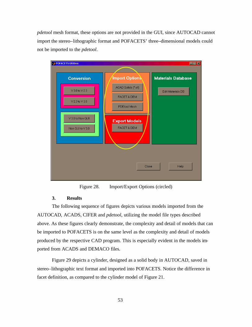
53

pdetool mesh format, these options are not provided in the GUI, since AUTOCAD cannot

import the stereo–lithographic format and POFACETS’ three–dimensional models could

not be imported to the pdetool.

Figure 28. Import/Export Options (circled)

3. Results

The following sequence of figures depicts various models imported from the

AUTOCAD, ACADS, CIFER and pdetool, utilizing the model file types described

above. As these figures clearly demonstrate, the complexity and detail of models that can

be imported to POFACETS is on the same level as the complexity and detail of models

produced by the respective CAD program. This is especially evident in the models im-

ported from ACADS and DEMACO files.

Figure 29 depicts a cylinder, designed as a solid body in AUTOCAD, saved in

stereo–lithographic text format and imported into POFACETS. Notice the difference in

facet definition, as compared to the cylinder model of Figure 21.

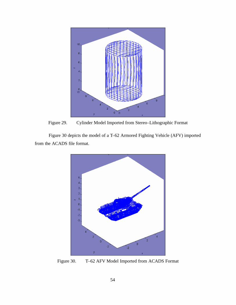
54

Figure 29. Cylinder Model Imported from Stereo–Lithographic Format

Figure 30 depicts the model of a T–62 Armored Fighting Vehicle (AFV) imported

from the ACADS file format.

Figure 30. T–62 AFV Model Imported from ACADS Format

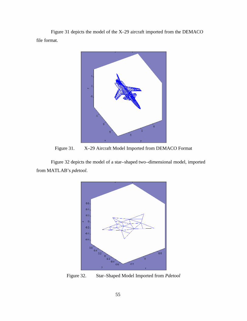
55

Figure 31 depicts the model of the X–29 aircraft imported from the DEMACO

file format.

Figure 31. X–29 Aircraft Model Imported from DEMACO Format

Figure 32 depicts the model of a star–shaped two–dimensional model, imported

from MATLAB’s pdetool.

Figure 32. Star–Shaped Model Imported from Pdetool

56

F. COMBINATION OF MODELS 1. Rationale

As discussed previously, the implementation of the Graphical Model Design GUI

and the development of code allowing the user to import into POFACETS models de-

signed in commercially available software provided significant versatility to the

POFACETS model management capabilities.

The next logical step was to provide code that would allow the combination of ex-

isting models. The goal here was twofold. First, a complex target model could be built by

combining simpler models. For example, a simple Unmanned Air Vehicle (UAV) can be

modeled through a combination of a fuselage, two trapezoidal wings and two parallelepi-

peds as stabilizers. Second, additional or optional parts could be added to a standard tar-

get model to evaluate the effects on its RCS. For example, the RCS of an aircraft could

be evaluated with or without external stores and armament.

2. Procedure

The combination of models is accomplished using the Graphical Model Design

GUI, through the Attach buttons, which are circled in Figure 33.

Figure 33. Model Combination (circled)

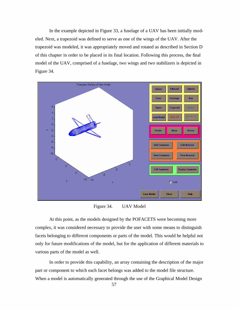
57

In the example depicted in Figure 33, a fuselage of a UAV has been initially mod-

eled. Next, a trapezoid was defined to serve as one of the wings of the UAV. After the

trapezoid was modeled, it was appropriately moved and rotated as described in Section D

of this chapter in order to be placed in its final location. Following this process, the final

model of the UAV, comprised of a fuselage, two wings and two stabilizers is depicted in

Figure 34.

Figure 34. UAV Model

At this point, as the models designed by the POFACETS were becoming more

complex, it was considered necessary to provide the user with some means to distinguish

facets belonging to different components or parts of the model. This would be helpful not

only for future modifications of the model, but for the application of different materials to

various parts of the model as well.

In order to provide this capability, an array containing the description of the major

part or component to which each facet belongs was added to the model file structure.

When a model is automatically generated through the use of the Graphical Model Design

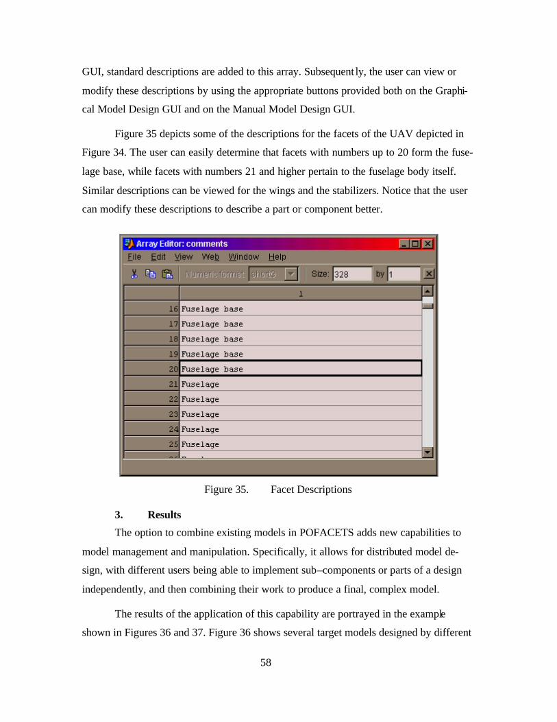
58

GUI, standard descriptions are added to this array. Subsequent ly, the user can view or

modify these descriptions by using the appropriate buttons provided both on the Graphi-

cal Model Design GUI and on the Manual Model Design GUI.

Figure 35 depicts some of the descriptions for the facets of the UAV depicted in

Figure 34. The user can easily determine that facets with numbers up to 20 form the fuse-

lage base, while facets with numbers 21 and higher pertain to the fuselage body itself.

Similar descriptions can be viewed for the wings and the stabilizers. Notice that the user

can modify these descriptions to describe a part or component better.

Figure 35. Facet Descriptions

3. Results

The option to combine existing models in POFACETS adds new capabilities to

model management and manipulation. Specifically, it allows for distributed model de-

sign, with different users being able to implement sub–components or parts of a design

independently, and then combining their work to produce a final, complex model.

The results of the application of this capability are portrayed in the example

shown in Figures 36 and 37. Figure 36 shows several target models designed by different

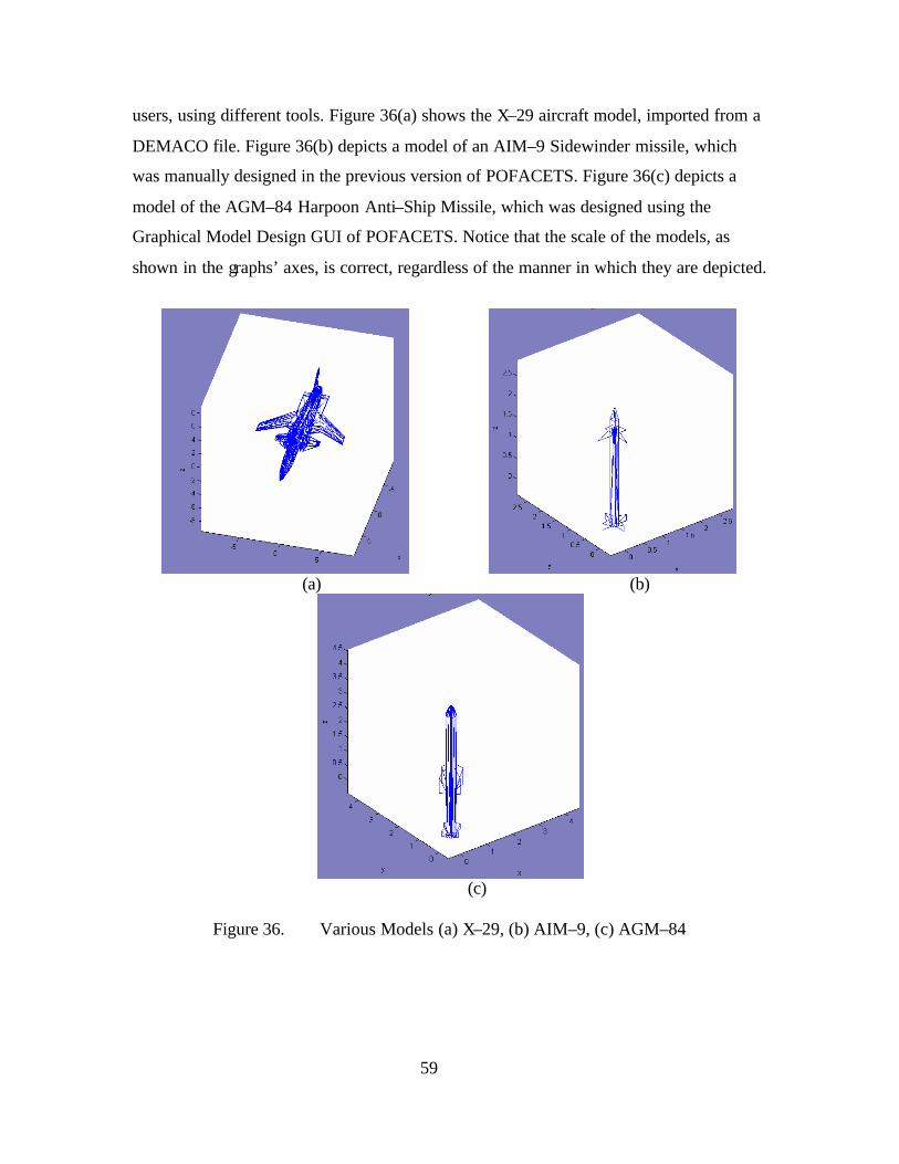
59

users, using different tools. Figure 36(a) shows the X–29 aircraft model, imported from a

DEMACO file. Figure 36(b) depicts a model of an AIM–9 Sidewinder missile, which

was manually designed in the previous version of POFACETS. Figure 36(c) depicts a

model of the AGM–84 Harpoon Anti–Ship Missile, which was designed using the

Graphical Model Design GUI of POFACETS. Notice that the scale of the models, as

shown in the graphs’ axes, is correct, regardless of the manner in which they are depicted.

(a)

(b)

(c)

Figure 36. Various Models (a) X–29, (b) AIM–9, (c) AGM–84

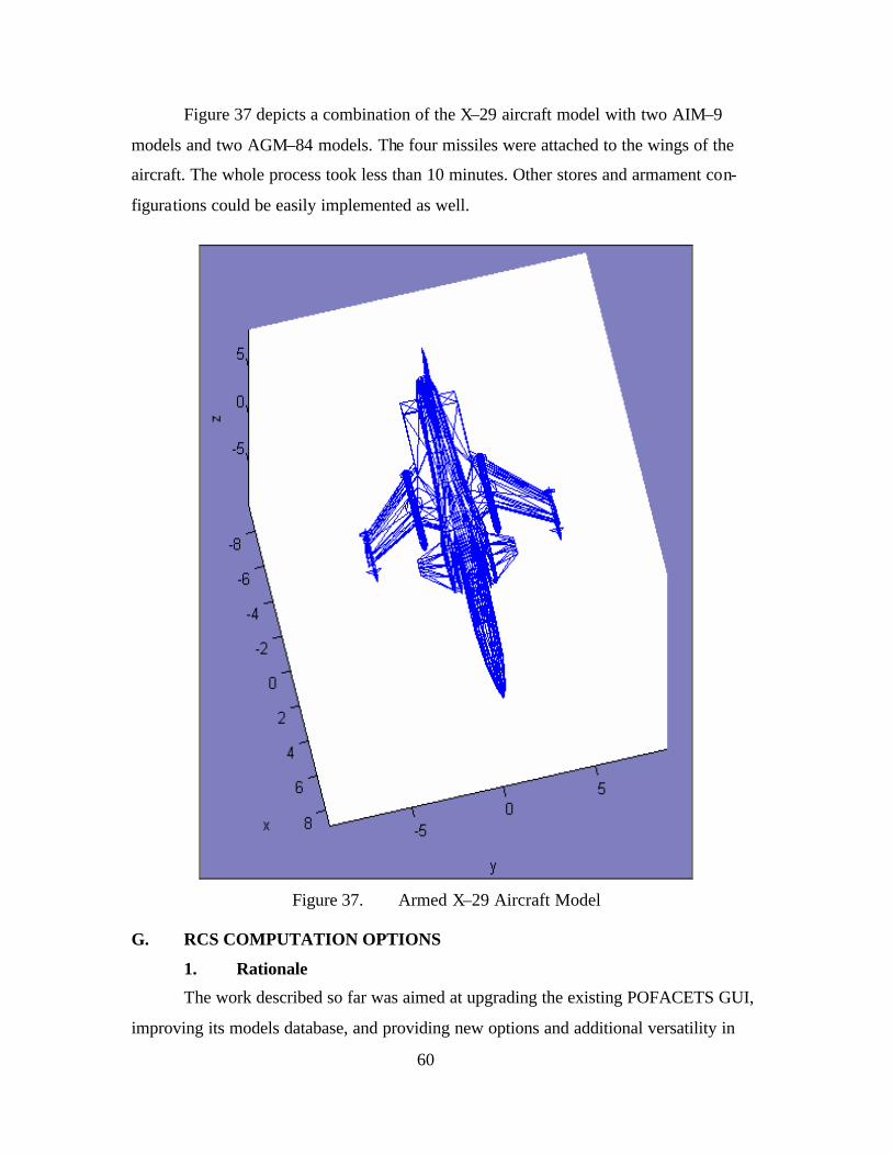
60

Figure 37 depicts a combination of the X–29 aircraft model with two AIM–9

models and two AGM–84 models. The four missiles were attached to the wings of the

aircraft. The whole process took less than 10 minutes. Other stores and armament con-

figurations could be easily implemented as well.

Figure 37. Armed X–29 Aircraft Model

G. RCS COMPUTATION OPTIONS

1. Rationale

The work described so far was aimed at upgrading the existing POFACETS GUI,

improving its models database, and providing new options and additional versatility in

61

the design of new models or the modification of existing models. All these features are

necessary in order to implement better and more efficiently the main goal of this pro-

gram, which is the prediction of the RCS of target models.

The POFACETS version 2.3 program provided the user with two main options

regarding the calculation of the RCS of a model, monostatic (i.e., the radar transmitter

and receiver are collocated) and bistatic (i.e., the radar transmitter and the radar receiver

are placed in different locations). The calculation of RCS was performed relative to the

spherical coordinates angles of observation, θ and φ , for a fixed frequency, which was

selected by the user. This type of RCS computation is the one that appears most often in

the relevant literature and, of course, it was maintained in the new POFACETS version,

with certain new computational capabilities being added, as described in the next chapter.

The monostatic and bistatic RCS computations were also expanded in the new

version of POFACETS to include the calculation of RCS versus frequency for a fixed,

user–selectable, observation angle. This option can be used to predict the RCS behavior

of a model over a selected range of frequencies, while it can also provide an additional

verification of RCS results obtained for standard targe t models.

2. Procedure and Results

a. RCS versus Observation Angles

The RCS computation versus the observation angles was implemented in

POFACETS version 2.3. Its GUIs are briefly discussed here, in order to provide a com-

plete description of the program’s functionalities. Figure 38 depicts the Monostatic RCS

Computation GUI.

First, the user selects and loads the model for which the RCS calculation

will be performed. The model is displayed, so that the user can review it and verify that

this is the desired model. Next, the user must select the parameters that will be used in the

RCS calculations. Specifically, the user enters values for the following parameters:

• Observation angle θ starting and ending values (from –360 to 360 de-grees), and increment value

• Observation angle φ starting and ending values (from –360 to 360 de-grees), and increment value

62

• Incident wave polarization (selectable between Transverse Magnetic and Transverse Electric)

• Frequency

• Taylor Series Number of Terms and Length of Region

• Surface Roughness Correlation Distance and Standard Deviation.

Many of these parameters have standard predefined values, so in those

cases, the user simply enters the desired frequency and observation angles. Notice that in

the case of observation angles, one of the two can be constant, as shown in Figure 38 for

the φ angle, resulting in a φ –cut or a θ –cut.

The user can also select to add a ground plane on the ( , )x y plane or ex-

ploit symmetry planes in the model (if any). These options are discussed in the next chap-

ter. Finally, the user can select the types of RCS plots that will be produced as a result of

the calculations.

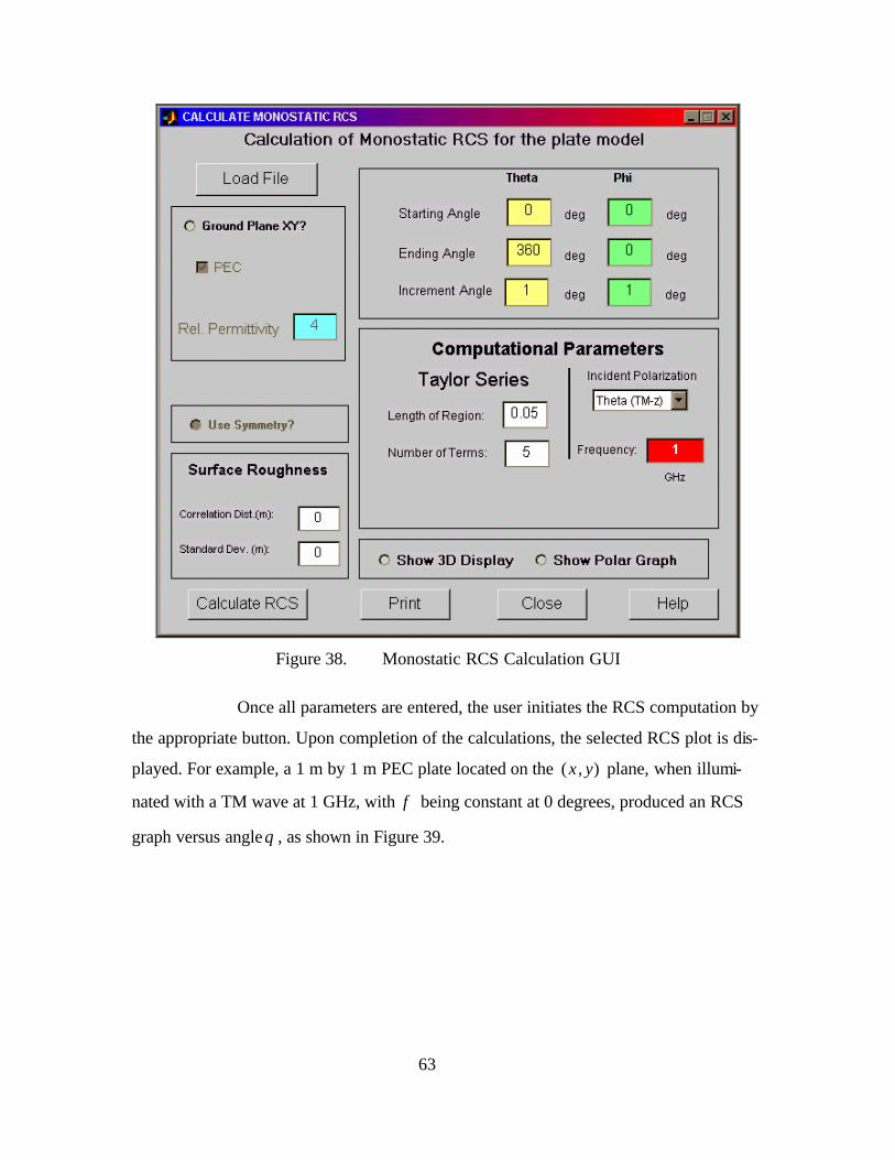
63

Figure 38. Monostatic RCS Calculation GUI

Once all parameters are entered, the user initiates the RCS computation by

the appropriate button. Upon completion of the calculations, the selected RCS plot is dis-

played. For example, a 1 m by 1 m PEC plate located on the ( , )x y plane, when illumi-

nated with a TM wave at 1 GHz, with φ being constant at 0 degrees, produced an RCS

graph versus angleθ , as shown in Figure 39.

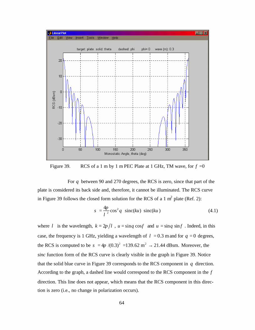
64

Figure 39. RCS of a 1 m by 1 m PEC Plate at 1 GHz, TM wave, for φ =0

For θ between 90 and 270 degrees, the RCS is zero, since that part of the

plate is considered its back side and, therefore, it cannot be illuminated. The RCS curve

in Figure 39 follows the closed form solution for the RCS of a 1 m2 plate (Ref. 2):

22

4cos sinc( ) sinc( )ku k

πσ θ υ

λ= ⋅ ⋅ (4.1)

where λ is the wavelength, 2k π λ= , sin cosu θ φ= and sin sinυ θ φ= . Indeed, in this

case, the frequency is 1 GHz, yielding a wavelength of 0.3 mλ = and for 0θ = degrees,

the RCS is computed to be 2 24 /(0.3) 139.62 m 21.44 dBsm.σ π= = → Moreover, the

sinc function form of the RCS curve is clearly visible in the graph in Figure 39. Notice

that the solid blue curve in Figure 39 corresponds to the RCS component in θ direction.

According to the graph, a dashed line would correspond to the RCS component in the φ

direction. This line does not appear, which means that the RCS component in this direc-

tion is zero (i.e., no change in polarization occurs).

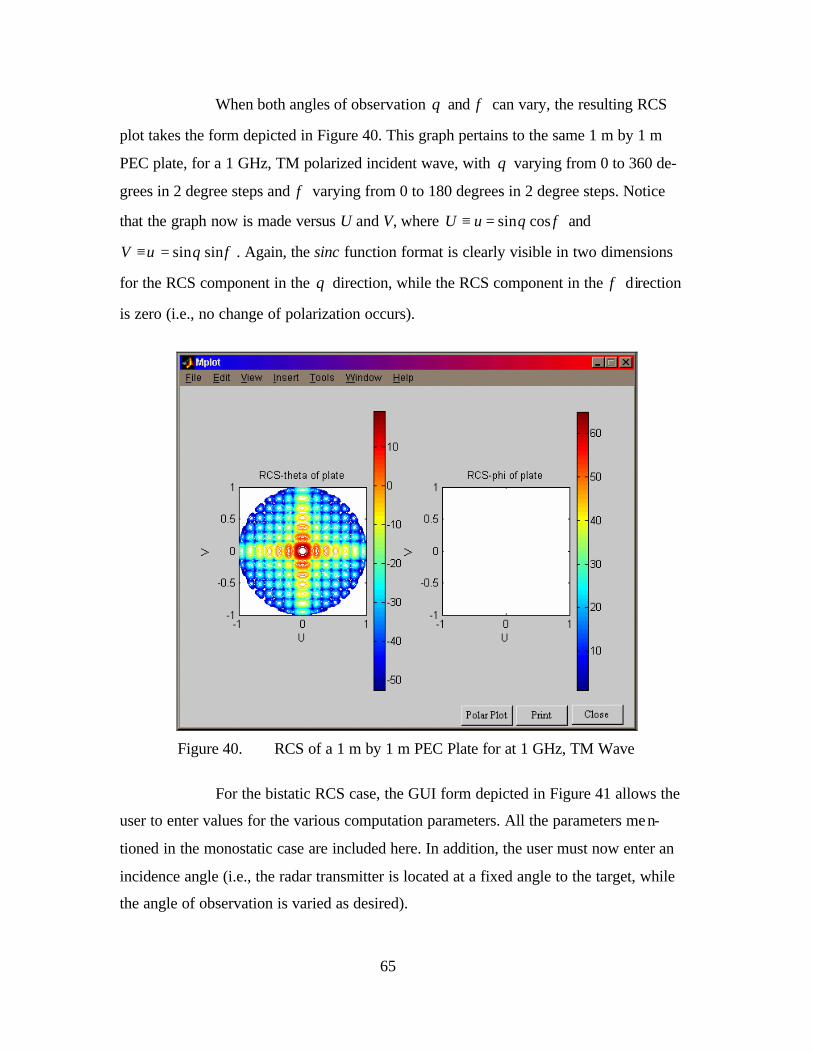
65

When both angles of observation θ and φ can vary, the resulting RCS

plot takes the form depicted in Figure 40. This graph pertains to the same 1 m by 1 m

PEC plate, for a 1 GHz, TM polarized incident wave, with θ varying from 0 to 360 de-

grees in 2 degree steps and φ varying from 0 to 180 degrees in 2 degree steps. Notice

that the graph now is made versus U and V, where sin cosU u θ φ≡ = and

sin sinV υ θ φ≡ = . Again, the sinc function format is clearly visible in two dimensions

for the RCS component in the θ direction, while the RCS component in the φ direction

is zero (i.e., no change of polarization occurs).

Figure 40. RCS of a 1 m by 1 m PEC Plate for at 1 GHz, TM Wave

For the bistatic RCS case, the GUI form depicted in Figure 41 allows the

user to enter values for the various computation parameters. All the parameters men-

tioned in the monostatic case are included here. In addition, the user must now enter an

incidence angle (i.e., the radar transmitter is located at a fixed angle to the target, while

the angle of observation is varied as desired).

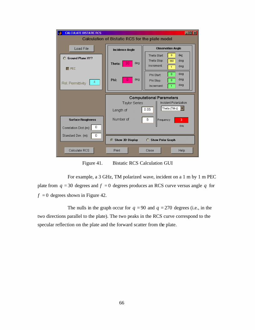
66

Figure 41. Bistatic RCS Calculation GUI

For example, a 3 GHz, TM polarized wave, incident on a 1 m by 1 m PEC

plate from 30θ = degrees and 0φ = degrees produces an RCS curve versus angle θ for

0φ = degrees shown in Figure 42.

The nulls in the graph occur for 90θ = and 270θ = degrees (i.e., in the

two directions parallel to the plate). The two peaks in the RCS curve correspond to the

specular reflection on the plate and the forward scatter from the plate.

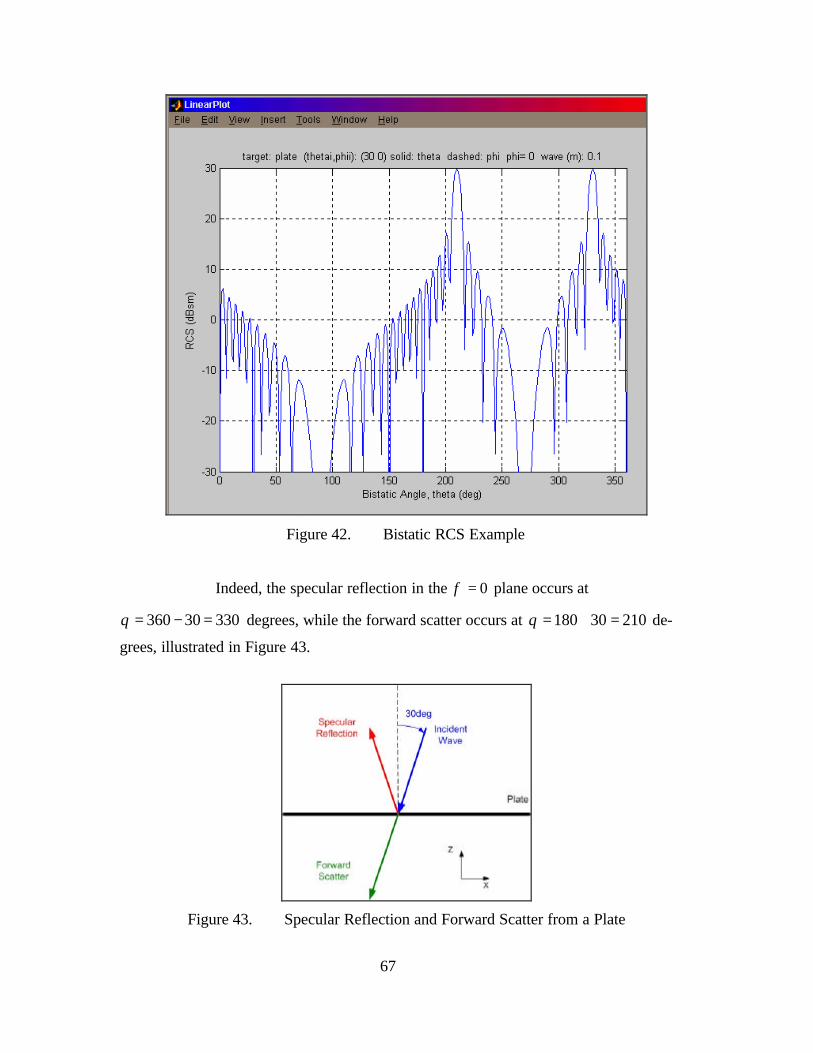
67

Figure 42. Bistatic RCS Example

Indeed, the specular reflection in the 0φ = plane occurs at

360 30 330θ = − = degrees, while the forward scatter occurs at 180 30 210θ = + = de-

grees, illustrated in Figure 43.

Figure 43. Specular Reflection and Forward Scatter from a Plate

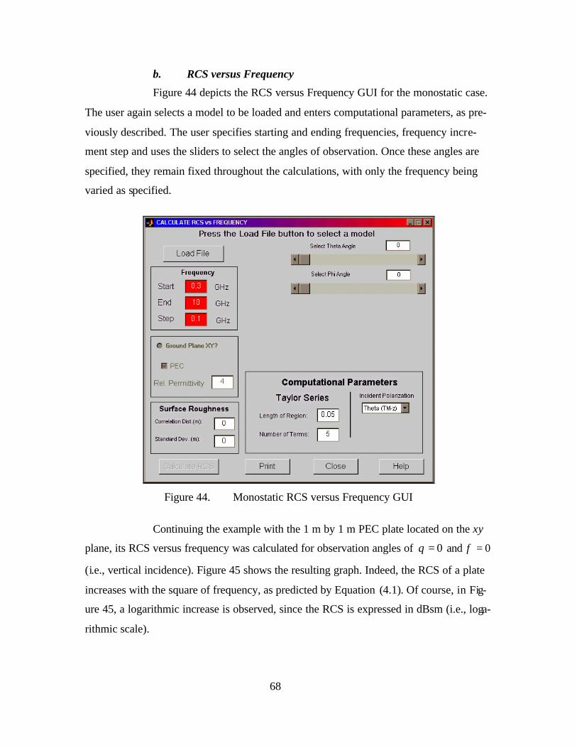
68

b. RCS versus Frequency

Figure 44 depicts the RCS versus Frequency GUI for the monostatic case.

The user again selects a model to be loaded and enters computational parameters, as pre-

viously described. The user specifies starting and ending frequencies, frequency incre-

ment step and uses the sliders to select the angles of observation. Once these angles are

specified, they remain fixed throughout the calculations, with only the frequency being

varied as specified.

Figure 44. Monostatic RCS versus Frequency GUI

Continuing the example with the 1 m by 1 m PEC plate located on the xy

plane, its RCS versus frequency was calculated for observation angles of 0θ = and 0φ =

(i.e., vertical incidence). Figure 45 shows the resulting graph. Indeed, the RCS of a plate

increases with the square of frequency, as predicted by Equation (4.1). Of course, in Fig-

ure 45, a logarithmic increase is observed, since the RCS is expressed in dBsm (i.e., loga-

rithmic scale).

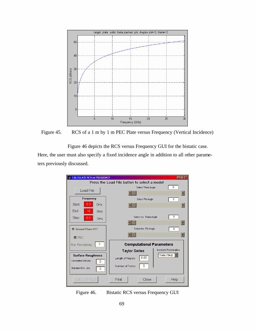
69

Figure 45. RCS of a 1 m by 1 m PEC Plate versus Frequency (Vertical Incidence)

Figure 46 depicts the RCS versus Frequency GUI for the bistatic case.

Here, the user must also specify a fixed incidence angle in addition to all other parame-

ters previously discussed.

Figure 46. Bistatic RCS versus Frequency GUI

70

H. RCS RESULTS DISPLAY OPTIONS

1. Rationale

Section G of this chapter presented the RCS displays of the POFACETS 2.3 ver-

sion. Two types of displays were available, depending on whether only one or both an-

gles θ and φ were used as parameters for RCS calculations. The displays were config-

ured to present a dynamic range of 60 dBsm. However, in some cases, this resulted in

small RCS values not being displayed at all (when the variations of the RCS exceeded 60

dBsm), while in other cases (when the variations of the RCS were in the order of 10 or 20

dBsm), details in the RCS plot were hard to detect.

Thus, the first improvement in the RCS display was to add a user–selectable dy-

namic range, so that the plot could be configured according to the users needs. This was

implemented for the plots in which one of the angles θ or φ was constant (i.e., not in the

contour of graphs like the one displayed in Figure 40).

Since the most common way to calculate the RCS of a target is versus angles θ ,

φ or both, a Polar Plot was added as an optional way to display the RCS, as angles are

more naturally represented in polar format.

Finally, a combination plot, which includes the target model superimposed on its

RCS, was added as an optional display. The goal was to illustrate how the incidence and

observation angles were related to the target and, thus, assist the user in performing

analysis of the RCS results and identifying the parts of the target that contribute to high

RCS values.

2. Procedure and Results

a. User–Selectable Dynamic Range

In order to allow the user to manually select the dynamic range that best

suits the RCS plot displayed, a slider was added in the GUI that presents the RCS plots in

the case when one of the angles θ or φ is constant. Figure 47 depicts the same results as

Figure 39 (i.e., RCS of a 1 m by 1 m PEC Plate at 1 GHz, TM wave, for φ =0 and θ

varying from 0 to 360 degrees). In this case, however, the dynamic range, as indicated by

the slider on the bottom of the GUI, was set to 100 dB. This resulted in less apparent dif-

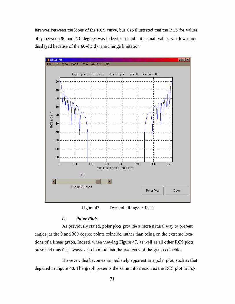
71

ferences between the lobes of the RCS curve, but also illustrated that the RCS for values

of θ between 90 and 270 degrees was indeed zero and not a small value, which was not

displayed because of the 60-dB dynamic range limitation.

Figure 47. Dynamic Range Effects

b. Polar Plots

As previously stated, polar plots provide a more natural way to present

angles, as the 0 and 360 degree points coincide, rather than being on the extreme loca-

tions of a linear graph. Indeed, when viewing Figure 47, as well as all other RCS plots

presented thus far, always keep in mind that the two ends of the graph coincide.

However, this becomes immediately apparent in a polar plot, such as that

depicted in Figure 48. The graph presents the same information as the RCS plot in Fig-

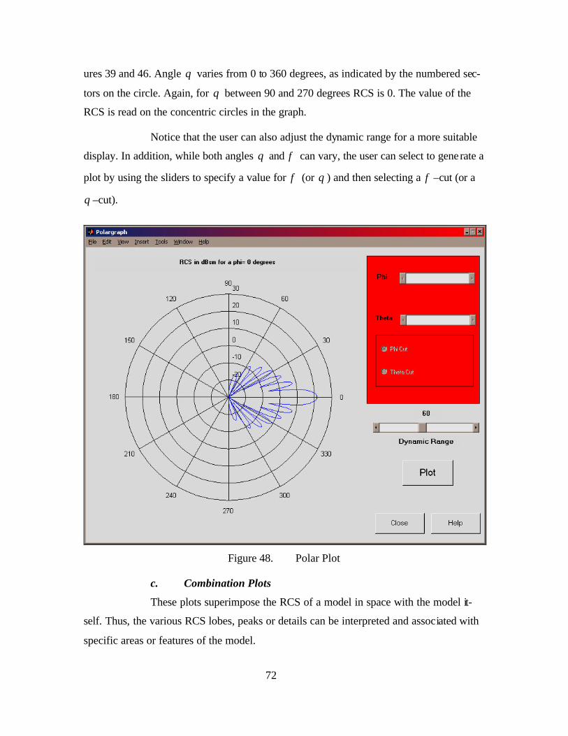
72

ures 39 and 46. Angle θ varies from 0 to 360 degrees, as indicated by the numbered sec-

tors on the circle. Again, for θ between 90 and 270 degrees RCS is 0. The value of the

RCS is read on the concentric circles in the graph.

Notice that the user can also adjust the dynamic range for a more suitable

display. In addition, while both angles θ and φ can vary, the user can select to generate a

plot by using the sliders to specify a value for φ (or θ ) and then selecting a φ –cut (or a

θ –cut).

Figure 48. Polar Plot

c. Combination Plots

These plots superimpose the RCS of a model in space with the model it-

self. Thus, the various RCS lobes, peaks or details can be interpreted and associated with

specific areas or features of the model.

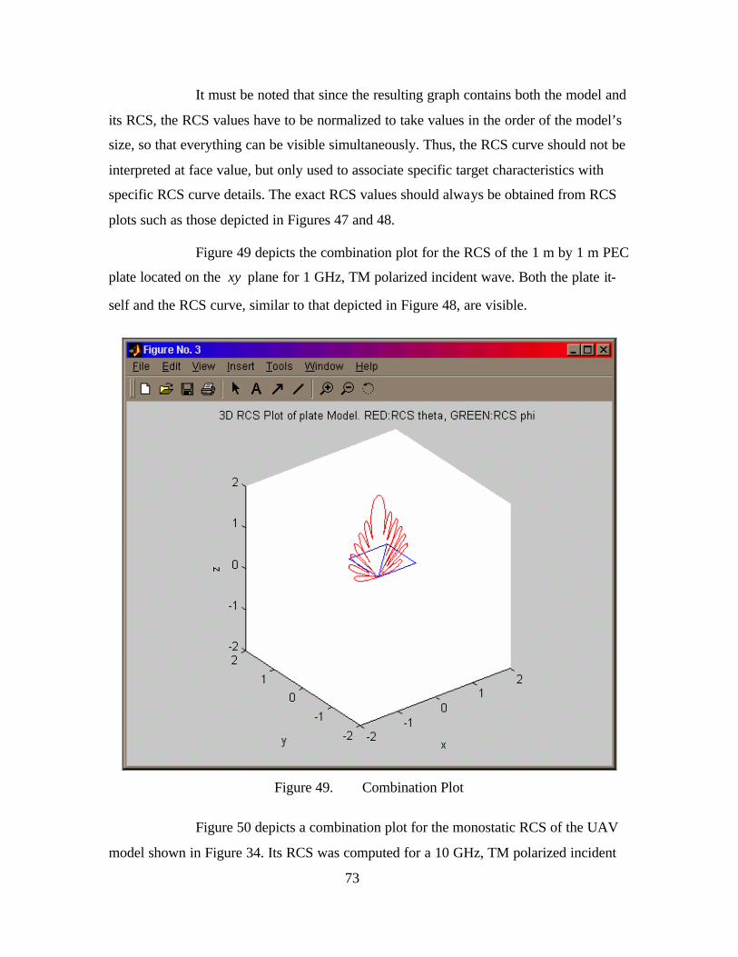
73

It must be noted that since the resulting graph contains both the model and

its RCS, the RCS values have to be normalized to take values in the order of the model’s

size, so that everything can be visible simultaneously. Thus, the RCS curve should not be

interpreted at face value, but only used to associate specific target characteristics with

specific RCS curve details. The exact RCS values should always be obtained from RCS

plots such as those depicted in Figures 47 and 48.

Figure 49 depicts the combination plot for the RCS of the 1 m by 1 m PEC

plate located on the xy plane for 1 GHz, TM polarized incident wave. Both the plate it-

self and the RCS curve, similar to that depicted in Figure 48, are visible.

Figure 49. Combination Plot

Figure 50 depicts a combination plot for the monostatic RCS of the UAV

model shown in Figure 34. Its RCS was computed for a 10 GHz, TM polarized incident

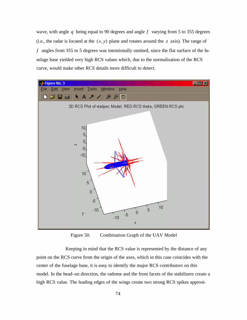
74

wave, with angle θ being equal to 90 degrees and angle φ varying from 5 to 355 degrees

(i.e., the radar is located at the ( , )x y plane and rotates around the z axis). The range of

φ angles from 355 to 5 degrees was intentionally omitted, since the flat surface of the fu-

selage base yielded very high RCS values which, due to the normalization of the RCS

curve, would make other RCS details more difficult to detect.

Figure 50. Combination Graph of the UAV Model

Keeping in mind that the RCS value is represented by the distance of any

point on the RCS curve from the origin of the axes, which in this case coincides with the

center of the fuselage base, it is easy to identify the major RCS contributors on this

model. In the head–on direction, the radome and the front facets of the stabilizers create a

high RCS value. The leading edges of the wings create two strong RCS spikes approxi-

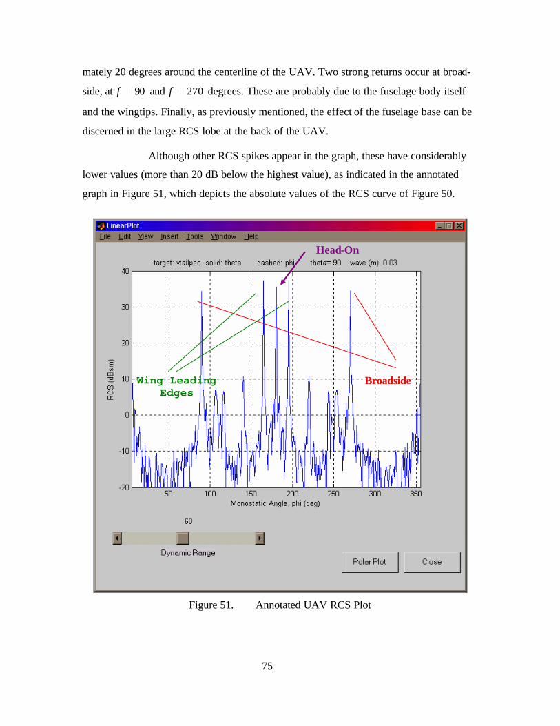
75

mately 20 degrees around the centerline of the UAV. Two strong returns occur at broad-

side, at 90φ = and 270φ = degrees. These are probably due to the fuselage body itself

and the wingtips. Finally, as previously mentioned, the effect of the fuselage base can be

discerned in the large RCS lobe at the back of the UAV.

Although other RCS spikes appear in the graph, these have considerably

lower values (more than 20 dB below the highest value), as indicated in the annotated

graph in Figure 51, which depicts the absolute values of the RCS curve of Figure 50.

Figure 51. Annotated UAV RCS Plot

Broadside

Head-On

Wing Leading Edges

76

I. SUMMARY

This chapter presented the improvements and the new functionalities incorporated

in the POFACETS. Specifically, the GUI and model database upgrade, the manual and

graphical model design options, the model import/export capabilities, the model combi-

nation capabilities, the RCS calculation options, and the RCS display options were de-

scribed. The following chapter discusses the new RCS computational capabilities of the

program.

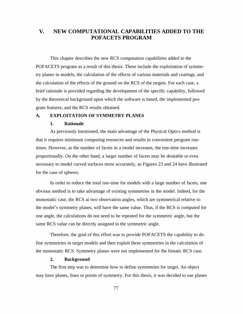
77

V. NEW COMPUTATIONAL CAPABILITIES ADDED TO THE POFACETS PROGRAM

This chapter describes the new RCS computation capabilities added to the

POFACETS program as a result of this thesis. These include the exploitation of symme-

try planes in models, the calculation of the effects of various materials and coatings, and

the calculation of the effects of the ground on the RCS of the targets. For each case, a

brief rationale is provided regarding the development of the specific capability, followed

by the theoretical background upon which the software is based, the implemented pro-

gram features, and the RCS results obtained.

A. EXPLOITATION OF SYMMETRY PLANES

1. Rationale

As previously mentioned, the main advantage of the Physical Optics method is

that it requires minimum computing resources and results in convenient program run–

times. However, as the number of facets in a model increases, the run–time increases

proportionally. On the other hand, a larger number of facets may be desirable or even

necessary to model curved surfaces more accurately, as Figures 23 and 24 have illustrated

for the case of spheres.

In order to reduce the total run–time for models with a large number of facets, one

obvious method is to take advantage of existing symmetries in the model. Indeed, for the

monostatic case, the RCS at two observation angles, which are symmetrical relative to

the model’s symmetry planes, will have the same value. Thus, if the RCS is computed for

one angle, the calculations do not need to be repeated for the symmetric angle, but the

same RCS value can be directly assigned to the symmetric angle.

Therefore, the goal of this effort was to provide POFACETS the capability to de-

fine symmetries in target models and then exploit these symmetries in the calculation of

the monostatic RCS. Symmetry planes were not implemented for the bistatic RCS case.

2. Background

The first step was to determine how to define symmetries for target. An object

may have planes, lines or points of symmetry. For this thesis, it was decided to use planes

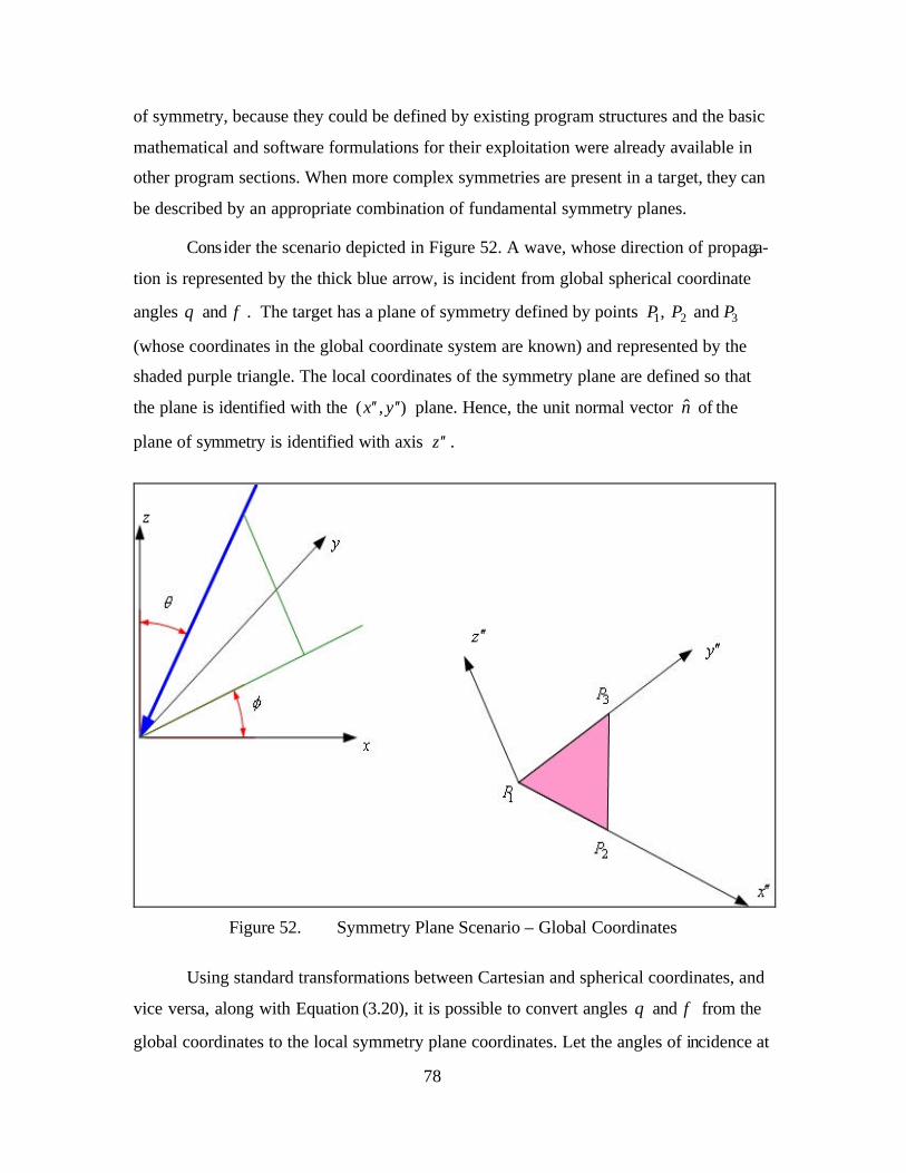
78

of symmetry, because they could be defined by existing program structures and the basic

mathematical and software formulations for their exploitation were already available in

other program sections. When more complex symmetries are present in a target, they can

be described by an appropriate combination of fundamental symmetry planes.

Consider the scenario depicted in Figure 52. A wave, whose direction of propaga-

tion is represented by the thick blue arrow, is incident from global spherical coordinate

angles θ and φ . The target has a plane of symmetry defined by points 1 2 3, and P P P

(whose coordinates in the global coordinate system are known) and represented by the

shaded purple triangle. The local coordinates of the symmetry plane are defined so that

the plane is identified with the ( , )x y′′ ′′ plane. Hence, the unit normal vector n of the

plane of symmetry is identified with axis z′′ .

Figure 52. Symmetry Plane Scenario – Global Coordinates

Using standard transformations between Cartesian and spherical coordinates, and

vice versa, along with Equation (3.20), it is possible to convert angles θ and φ from the

global coordinates to the local symmetry plane coordinates. Let the angles of incidence at

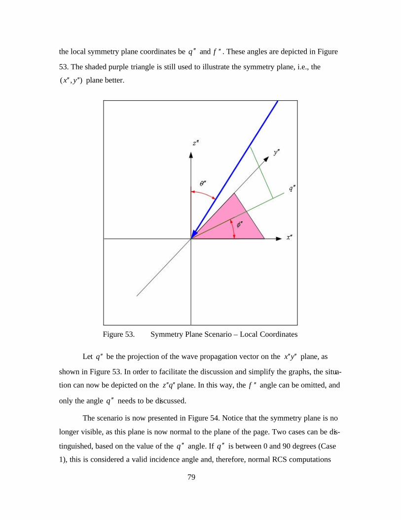
79

the local symmetry plane coordinates be θ ′′ and φ ′′ . These angles are depicted in Figure

53. The shaded purple triangle is still used to illustrate the symmetry plane, i.e., the

( , )x y′′ ′′ plane better.

Figure 53. Symmetry Plane Scenario – Local Coordinates

Let q′′ be the projection of the wave propagation vector on the x y′′ ′′ plane, as

shown in Figure 53. In order to facilitate the discussion and simplify the graphs, the situa-

tion can now be depicted on the z q′′ ′′ plane. In this way, the φ ′′ angle can be omitted, and

only the angle θ ′′ needs to be discussed.

The scenario is now presented in Figure 54. Notice that the symmetry plane is no

longer visible, as this plane is now normal to the plane of the page. Two cases can be dis-

tinguished, based on the value of the θ ′′ angle. If θ ′′ is between 0 and 90 degrees (Case

1), this is considered a valid incidence angle and, therefore, normal RCS computations

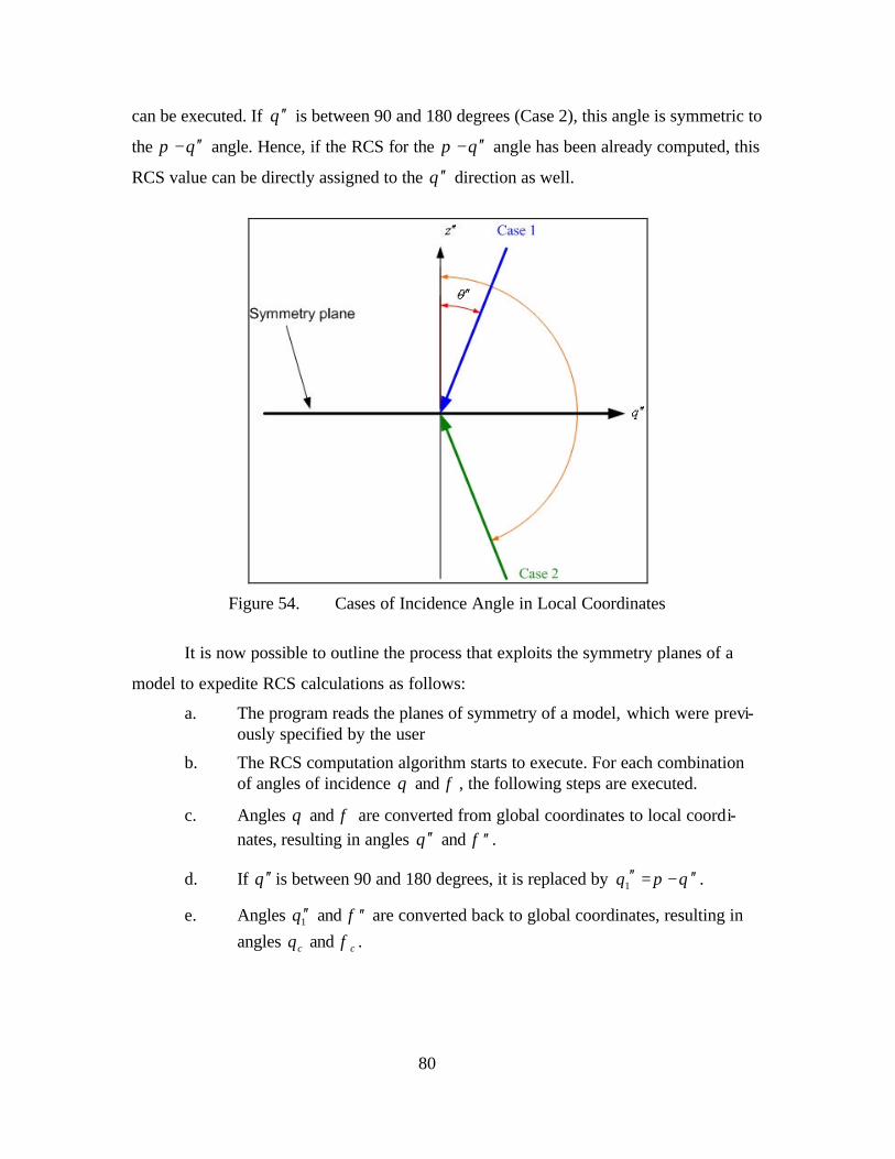
80

can be executed. If θ ′′ is between 90 and 180 degrees (Case 2), this angle is symmetric to

the π θ ′′− angle. Hence, if the RCS for the π θ ′′− angle has been already computed, this

RCS value can be directly assigned to the θ ′′ direction as well.

Figure 54. Cases of Incidence Angle in Local Coordinates

It is now possible to outline the process that exploits the symmetry planes of a

model to expedite RCS calculations as follows:

a. The program reads the planes of symmetry of a model, which were previ-ously specified by the user

b. The RCS computation algorithm starts to execute. For each combination of angles of incidence θ and φ , the following steps are executed.

c. Angles θ and φ are converted from global coordinates to local coordi-nates, resulting in angles θ ′′ and φ ′′ .

d. If θ ′′ is between 90 and 180 degrees, it is replaced by 1θ π θ′′ ′′= − .

e. Angles 1θ ′′ and φ ′′ are converted back to global coordinates, resulting in angles cθ and cφ .

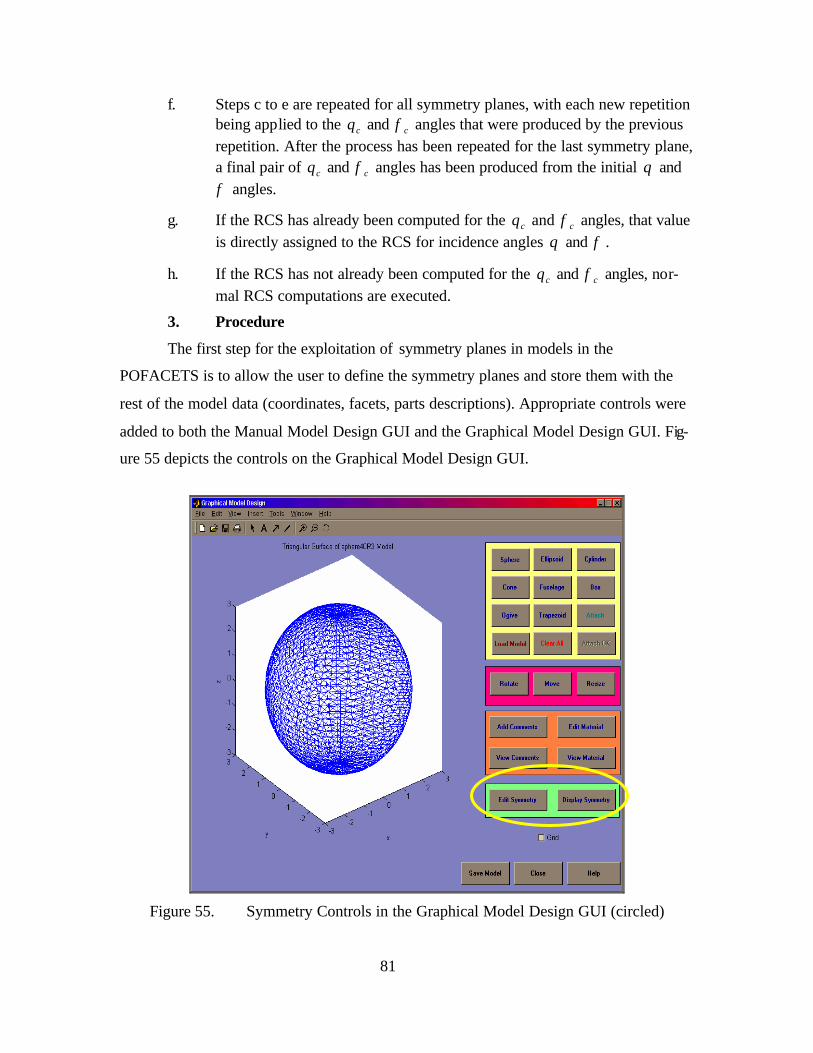
81

f. Steps c to e are repeated for all symmetry planes, with each new repetition being applied to the cθ and cφ angles that were produced by the previous repetition. After the process has been repeated for the last symmetry plane, a final pair of cθ and cφ angles has been produced from the initial θ and φ angles.

g. If the RCS has already been computed for the cθ and cφ angles, that value is directly assigned to the RCS for incidence angles θ and φ .

h. If the RCS has not already been computed for the cθ and cφ angles, nor-mal RCS computations are executed.

3. Procedure

The first step for the exploitation of symmetry planes in models in the

POFACETS is to allow the user to define the symmetry planes and store them with the

rest of the model data (coordinates, facets, parts descriptions). Appropriate controls were

added to both the Manual Model Design GUI and the Graphical Model Design GUI. Fig-

ure 55 depicts the controls on the Graphical Model Design GUI.

Figure 55. Symmetry Controls in the Graphical Model Design GUI (circled)

82

The user describes each symmetry plane using MATLAB’s array editor by enter-

ing three points for each symmetry plane. Figure 56 depicts an array of points defining

three symmetry planes. Each column represents the coordinates of a point in x, y, and z.

Each row represents a point, and each group of three rows represents a symmetry plane.

The sequence by which each plane is defined follows the right–hand rule, so that the right

hand points to the outward normal of the plane. Up to three symmetry planes can be de-

fined for each model.

Figure 56. Symmetry Plane Definition

Once the symmetry planes have been defined, they are superimposed on the

model display in the form of triangles of different colors. Figure 57 shows the three

symmetry planes for a sphere model with a radius of 3 m and 40 points per circle.

83

Figure 57. Symmetry Planes for a Sphere Model

When a model that contains symmetry planes is loaded for the computation of its

monostatic RCS, the Use Symmetry checkbox in the Monostatic RCS Calculation GUI is

enabled, as shown in Figure 58. If no symmetry planes exist, the checkbox remains dis-

abled.

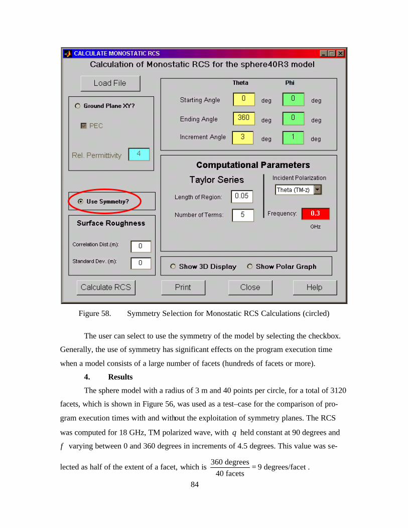
84

Figure 58. Symmetry Selection for Monostatic RCS Calculations (circled)

The user can select to use the symmetry of the model by selecting the checkbox.

Generally, the use of symmetry has significant effects on the program execution time

when a model consists of a large number of facets (hundreds of facets or more).

4. Results

The sphere model with a radius of 3 m and 40 points per circle, for a total of 3120

facets, which is shown in Figure 56, was used as a test–case for the comparison of pro-

gram execution times with and without the exploitation of symmetry planes. The RCS

was computed for 18 GHz, TM polarized wave, with θ held constant at 90 degrees and

φ varying between 0 and 360 degrees in increments of 4.5 degrees. This value was se-

lected as half of the extent of a facet, which is 360 degrees

9 degrees/facet40 facets

= .

85

Both executions, with and without exploitation of the symmetry planes, gave the

same RCS results, shown in Figure 59. The fluctuations between the two values are ex-

pected, since even and odd multiples of the 4.5 degrees increment step result in slightly

different configuration of facets being illuminated by the incident wave.

Figure 59. Monostatic RCS of a Sphere with Radius of 3 m at 18 GHz

When the program was run without exploitation of symmetry planes, it was com-

pleted in 130 seconds. When using the symmetry planes, the RCS computations were

executed in 35 seconds, resulting in a decrease of 73% in run–time.

B. EFFECTS OF MATERIALS AND COATINGS ON RCS

1. Rationale

The POFACETS 2.3 version allowed the user to use different materials on the

facets of a model by specifying the value of the surface resistivity sR for each facet. This

86

meant that, since the known parameters for any material are its constitutive parameters

(i.e., its relative electric permittivity and its relative magnetic permeability), the user

would have to use these parameters to calculate the surface resistivity in order to enter it

in the program. These calculations would have to be performed each time a new material

was used in a model. Moreover, it would be very difficult to implement more complex

configurations of facet materials, such as multiple layers and coatings on PEC.

Therefore, it was decided to add the necessary features to POFACETS to allow

the user to directly select materials for the facets of the model (utilizing the material de-

scription) and provide different options regarding the application of these materials to the

model. These options include single composite material, composite material layer on

PEC, multiple composite layers and multiple composite layers on PEC. These are suffi-

cient to account for most of the usual cases of materials on “real–world” targets.

For the convenience of the user, a database of materials has been created that in-

cludes the description of common materials and their constitutive parameters. The user

can also update the database to include new types of material.

2. Background

As previously mentioned, the program allows four different types of material con-

figurations for a facet: (1) single composite material, (2) composite material layer on

PEC, (3) multiple composite layers, and (4) multiple composite layers on PEC. The theo-

retical framework for each of these cases is discussed below. The discussion begins from

the multiple composite layers case and the composite layer on PEC case. The formulas

for the other two cases are derived as special cases of the formulas of the first two cases.

For each case, the goal is to compute the reflection coefficients for parallel and perpen-

dicular polarization, so that they can be directly used in Equations (3.30) and (3.31).

Notice that the electric permittivity is

( ) ( )tanr r r r rj jο ο οε ε ε ε ε ε ε ε ε δ′ ′′ ′ ′= = − = − (5.1)

where oε is the electric permittivity of free space, rε′ the real part of the relative electric

permittivity of the material and tanδ the electric loss tangent of the material. Similarly,

the magnetic permeability of the material is

87

( )r r rjο οµ µ µ µ µ µ′ ′′= = − (5.2)

where oµ is the magnetic permeability of free space, rµ′ the real part of the relative mag-

netic permeability of the material and rµ′′ the imaginary part of the relative magnetic

permeability of the material.

a. Case 1: Multiple Composite Layers

Consider the configuration shown in Figure 60. A wave represented by 1c ,

traveling to the positive z direction, is incident on a body comprised of N different layers.

The material in front of layer 1 is free space. The constitutive parameters of layer n are

nε (electric permittivity) and nµ (magnetic permeability). The thickness of each layer is

nt . Symbols c and b represent the waves incident and reflected at each boundary, respec-

tively. The reflection coefficient between region 0 (i.e., free space) and region 1 is 1Γ ,

while the reflection coefficient between region 1n − and region n is nΓ . Similarly, the

transmission coefficient between region 0 (i.e., free space) and region 1 is 1τ , while the

transmission coefficient between region 1n − and region n is nτ .

Figure 60. Wave Incident on Multiple Layers (After Ref. 8.)

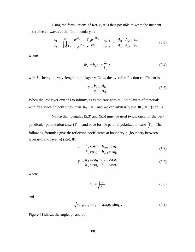
88

Using the formulations of Ref. 8, it is thus possible to write the incident

and reflected waves at the first boundary as

1 11 11 12

1 1 21 22 11

1

n n

n n

j jNN Nn

j jN Nnn n

c cc A Ae eb b A A be eτ

Φ − Φ+ +

Φ − Φ+ +=

Γ = ≡

Γ ∏ (5.3)

where

2

n n n nn

t tπ

βλ

Φ = = (5.4)

with nλ being the wavelength in the layer n. Now, the overall reflection coefficient is

1 21

1 11

b Ac A

Γ = = . (5.5)

When the last layer extends to infinity, as is the case with multiple layers of materials

with free space on both sides, then 1 0Nb + = and we can arbitrarily use 0NΦ = (Ref. 8).

Notice that formulas (5.3) and (5.5) must be used twice: once for the per-

pendicular polarization case ( )⊥Γ and once for the parallel polarization case ( )ΓP The

following formulas give the reflection coefficients at boundary n (boundary between

layer n–1 and layer n) (Ref. 8):

1

1

cos coscos cos

n i n t

n i n t

η θ η θη θ η θ

−⊥

−

−Γ =

+ (5.6)

1

1

cos coscos cos

n t n i

n t n i

η θ η θη θ η θ

−

−

−Γ =

+P (5.7)

where

nn

n

µη

ε= (5.8)

and

1 1 sin sinn n i n n tµ ε θ µ ε θ− − = . (5.9)

Figure 61 shows the angles and i tθ θ .

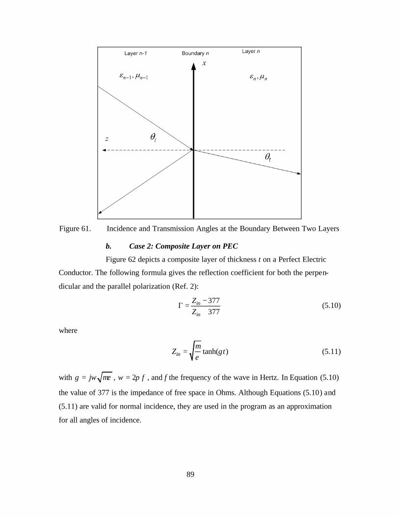
89

Figure 61. Incidence and Transmission Angles at the Boundary Between Two Layers

b. Case 2: Composite Layer on PEC

Figure 62 depicts a composite layer of thickness t on a Perfect Electric

Conductor. The following formula gives the reflection coefficient for both the perpen-

dicular and the parallel polarization (Ref. 2):

377377

in

in

ZZ

−Γ =

+ (5.10)

where

tanh( )inZ tµ

γε

= (5.11)

with jγ ω µε= , 2 fω π= , and f the frequency of the wave in Hertz. In Equation (5.10)

the value of 377 is the impedance of free space in Ohms. Although Equations (5.10) and

(5.11) are valid for normal incidence, they are used in the program as an approximation

for all angles of incidence.

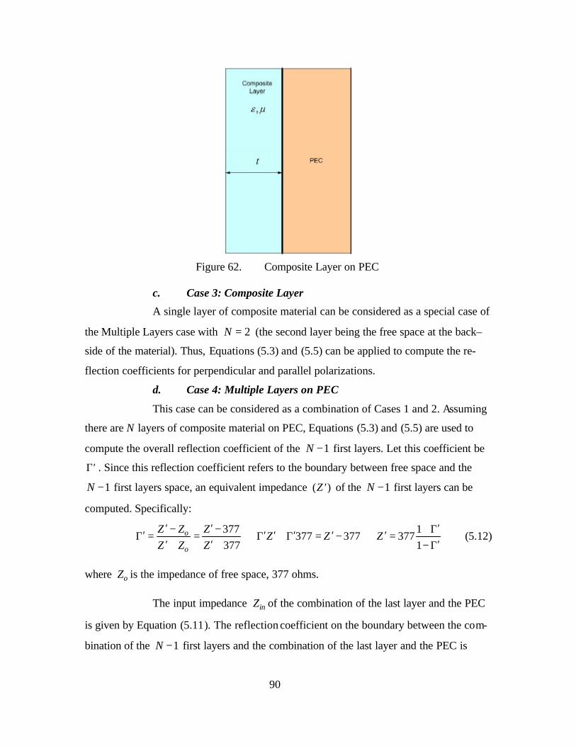
90

Figure 62. Composite Layer on PEC

c. Case 3: Composite Layer

A single layer of composite material can be considered as a special case of

the Multiple Layers case with 2N = (the second layer being the free space at the back–

side of the material). Thus, Equations (5.3) and (5.5) can be applied to compute the re-

flection coefficients for perpendicular and parallel polarizations.

d. Case 4: Multiple Layers on PEC

This case can be considered as a combination of Cases 1 and 2. Assuming

there are N layers of composite material on PEC, Equations (5.3) and (5.5) are used to

compute the overall reflection coefficient of the 1N − first layers. Let this coefficient be

′Γ . Since this reflection coefficient refers to the boundary between free space and the

1N − first layers space, an equivalent impedance ( )Z ′ of the 1N − first layers can be

computed. Specifically:

377 1

377 377 377377 1

o

o

Z Z ZZ Z Z

Z Z Z′ ′ ′− − + Γ′ ′ ′ ′ ′ ′Γ = = ⇒ Γ + Γ = − ⇒ =′ ′ ′+ + − Γ

(5.12)

where oZ is the impedance of free space, 377 ohms.

The input impedance inZ of the combination of the last layer and the PEC

is given by Equation (5.11). The reflection coefficient on the boundary between the com-

bination of the 1N − first layers and the combination of the last layer and the PEC is

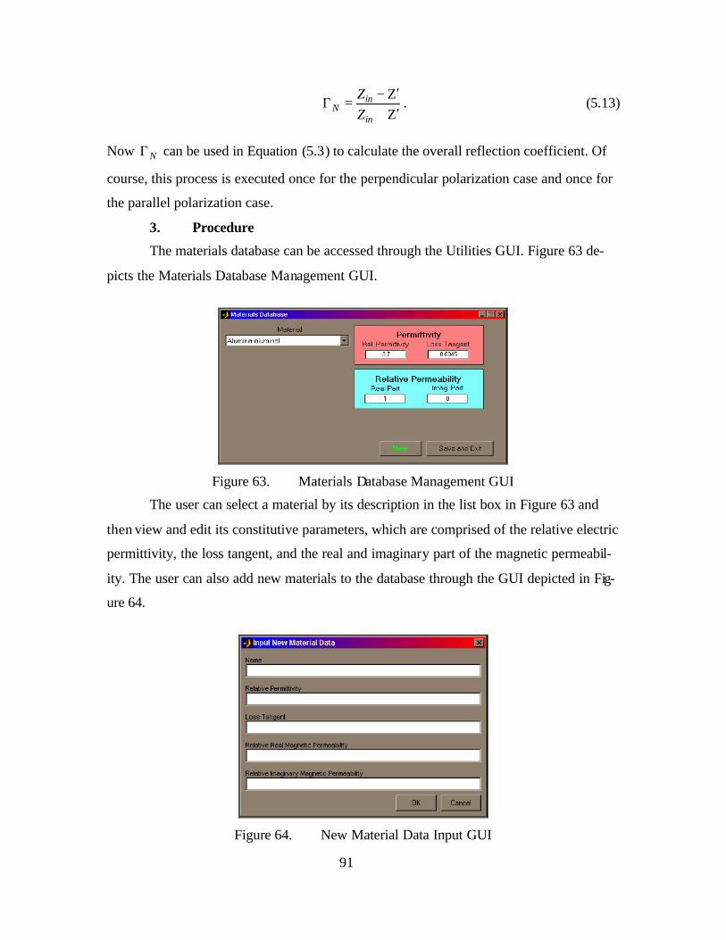
91

inN

in

ZZ

′− ΖΓ =

′+ Ζ. (5.13)

Now NΓ can be used in Equation (5.3) to calculate the overall reflection coefficient. Of

course, this process is executed once for the perpendicular polarization case and once for

the parallel polarization case.

3. Procedure

The materials database can be accessed through the Utilities GUI. Figure 63 de-

picts the Materials Database Management GUI.

Figure 63. Materials Database Management GUI

The user can select a material by its description in the list box in Figure 63 and

then view and edit its constitutive parameters, which are comprised of the relative electric

permittivity, the loss tangent, and the real and imaginary part of the magnetic permeabil-

ity. The user can also add new materials to the database through the GUI depicted in Fig-

ure 64.

Figure 64. New Material Data Input GUI

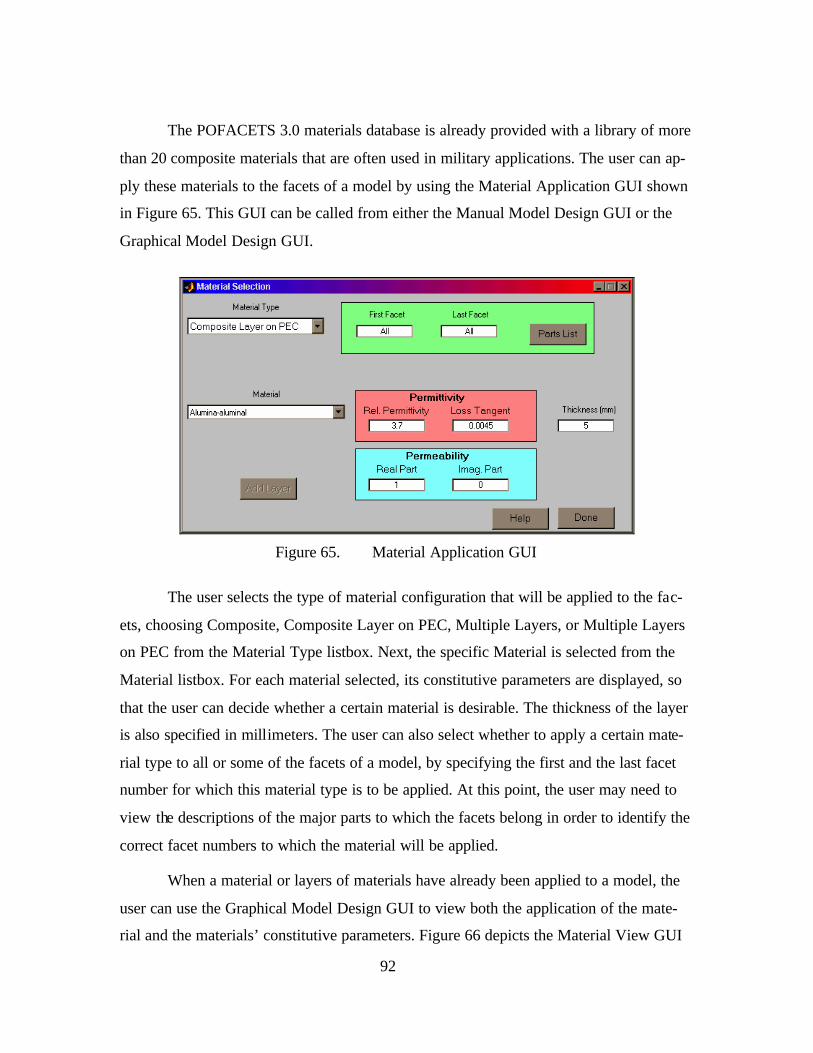
92

The POFACETS 3.0 materials database is already provided with a library of more

than 20 composite materials that are often used in military applications. The user can ap-

ply these materials to the facets of a model by using the Material Application GUI shown

in Figure 65. This GUI can be called from either the Manual Model Design GUI or the

Graphical Model Design GUI.

Figure 65. Material Application GUI

The user selects the type of material configuration that will be applied to the fac-

ets, choosing Composite, Composite Layer on PEC, Multiple Layers, or Multiple Layers

on PEC from the Material Type listbox. Next, the specific Material is selected from the

Material listbox. For each material selected, its constitutive parameters are displayed, so

that the user can decide whether a certain material is desirable. The thickness of the layer

is also specified in millimeters. The user can also select whether to apply a certain mate-

rial type to all or some of the facets of a model, by specifying the first and the last facet

number for which this material type is to be applied. At this point, the user may need to

view the descriptions of the major parts to which the facets belong in order to identify the

correct facet numbers to which the material will be applied.

When a material or layers of materials have already been applied to a model, the

user can use the Graphical Model Design GUI to view both the application of the mate-

rial and the materials’ constitutive parameters. Figure 66 depicts the Material View GUI

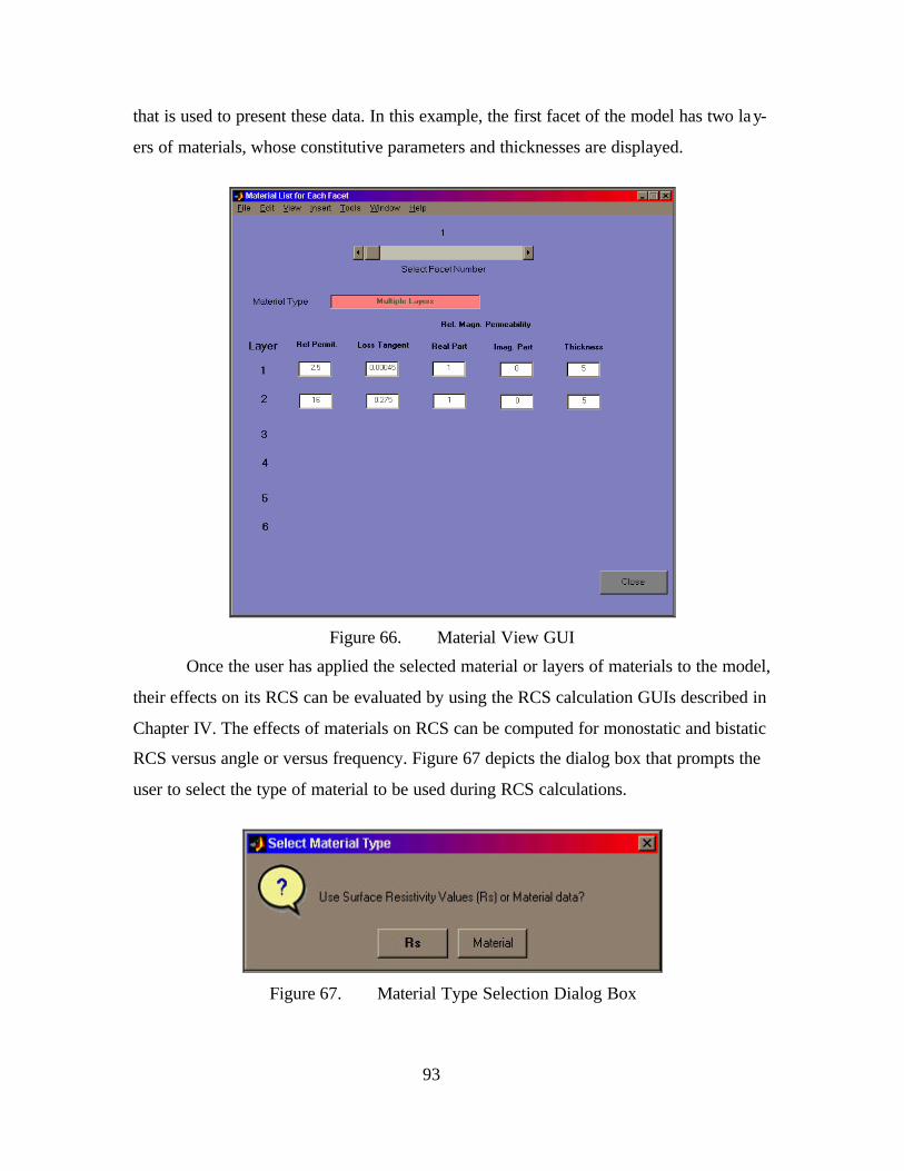
93

that is used to present these data. In this example, the first facet of the model has two lay-

ers of materials, whose constitutive parameters and thicknesses are displayed.

Figure 66. Material View GUI

Once the user has applied the selected material or layers of materials to the model,

their effects on its RCS can be evaluated by using the RCS calculation GUIs described in

Chapter IV. The effects of materials on RCS can be computed for monostatic and bistatic

RCS versus angle or versus frequency. Figure 67 depicts the dialog box that prompts the

user to select the type of material to be used during RCS calculations.

Figure 67. Material Type Selection Dialog Box

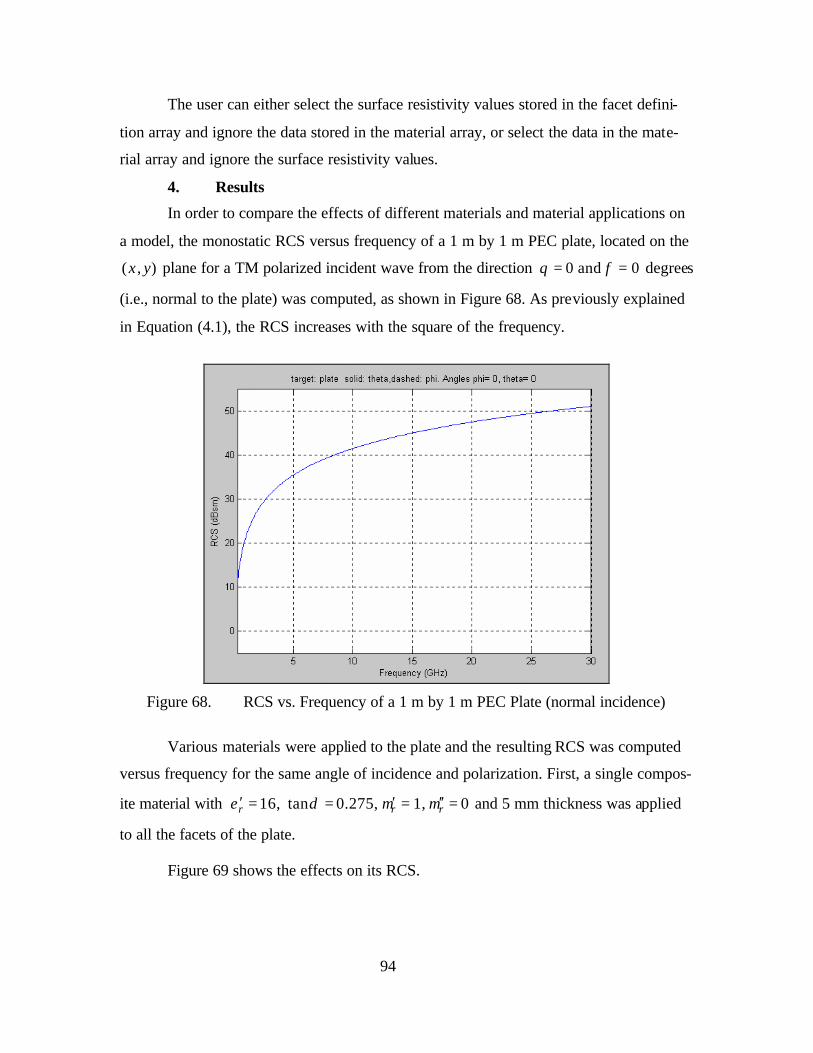
94

The user can either select the surface resistivity values stored in the facet defini-

tion array and ignore the data stored in the material array, or select the data in the mate-

rial array and ignore the surface resistivity values.

4. Results

In order to compare the effects of different materials and material applications on

a model, the monostatic RCS versus frequency of a 1 m by 1 m PEC plate, located on the

( , )x y plane for a TM polarized incident wave from the direction 0 and 0θ φ= = degrees

(i.e., normal to the plate) was computed, as shown in Figure 68. As previously explained

in Equation (4.1), the RCS increases with the square of the frequency.

Figure 68. RCS vs. Frequency of a 1 m by 1 m PEC Plate (normal incidence)

Various materials were applied to the plate and the resulting RCS was computed

versus frequency for the same angle of incidence and polarization. First, a single compos-

ite material with 16, tan 0.275, 1, 0r r rε δ µ µ′ ′ ′′= = = = and 5 mm thickness was applied

to all the facets of the plate.

Figure 69 shows the effects on its RCS.

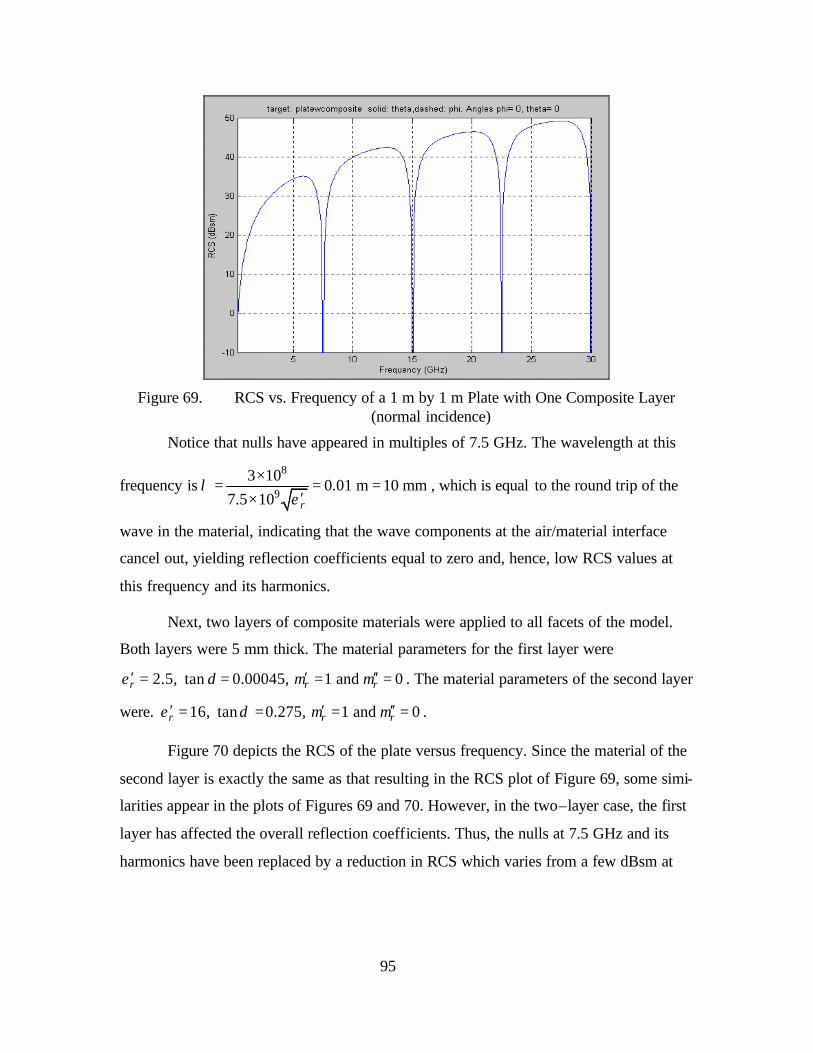
95

Figure 69. RCS vs. Frequency of a 1 m by 1 m Plate with One Composite Layer

(normal incidence)

Notice that nulls have appeared in multiples of 7.5 GHz. The wavelength at this

frequency is8

9

3 100.01 m 10 mm

7.5 10 r

λε

×= = =

′×, which is equal to the round trip of the

wave in the material, indicating that the wave components at the air/material interface

cancel out, yielding reflection coefficients equal to zero and, hence, low RCS values at

this frequency and its harmonics.

Next, two layers of composite materials were applied to all facets of the model.

Both layers were 5 mm thick. The material parameters for the first layer were

2.5, tan 0.00045, 1 and 0r r rε δ µ µ′ ′ ′′= = = = . The material parameters of the second layer

were. 16, tan 0.275, 1 and 0r r rε δ µ µ′ ′ ′′= = = = .

Figure 70 depicts the RCS of the plate versus frequency. Since the material of the

second layer is exactly the same as that resulting in the RCS plot of Figure 69, some simi-

larities appear in the plots of Figures 69 and 70. However, in the two–layer case, the first

layer has affected the overall reflection coefficients. Thus, the nulls at 7.5 GHz and its

harmonics have been replaced by a reduction in RCS which varies from a few dBsm at

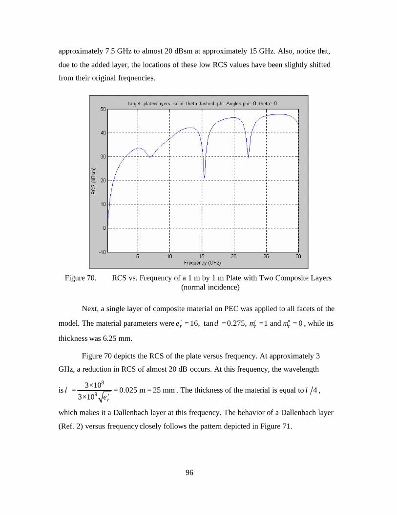
96

approximately 7.5 GHz to almost 20 dBsm at approximately 15 GHz. Also, notice that,

due to the added layer, the locations of these low RCS values have been slightly shifted

from their original frequencies.

Figure 70. RCS vs. Frequency of a 1 m by 1 m Plate with Two Composite Layers

(normal incidence)

Next, a single layer of composite material on PEC was applied to all facets of the

model. The material parameters were 16, tan 0.275, 1 and 0r r rε δ µ µ′ ′ ′′= = = = , while its

thickness was 6.25 mm.

Figure 70 depicts the RCS of the plate versus frequency. At approximately 3

GHz, a reduction in RCS of almost 20 dB occurs. At this frequency, the wavelength

is8

9

3 100.025 m 25 mm

3 10 r

λε

×= = =

′×. The thickness of the material is equal to 4λ ,

which makes it a Dallenbach layer at this frequency. The behavior of a Dallenbach layer

(Ref. 2) versus frequency closely follows the pattern depicted in Figure 71.

97

Figure 71. RCS vs. Frequency of a 1 m by 1 m Plate with One Composite Layer on

PEC (normal incidence)

Finally, two layers of composite materials on PEC were applied to all the facets of

the model. The first layer was 5 mm thick and its material constitutive parameters

were 2.5, tan 0.00045, 1 and 0r r rε δ µ µ′ ′ ′′= = = = . The second layer was 6.25 mm thick

and its parameters were 16, tan 0.275, 1 and 0r r rε δ µ µ′ ′ ′′= = = = .

Figure 72 depicts the RCS of the plate versus frequency. The existence of two

layers significantly affects the RCS of the plate. The reduction in RCS at 3 GHz is now

approximately 15 dB. However, there is a reduction of approximately 25 dB in the RCS

at 9 GHz. The reduction of RCS at this frequency was approximately 5 dB for the single

layer on PEC case.

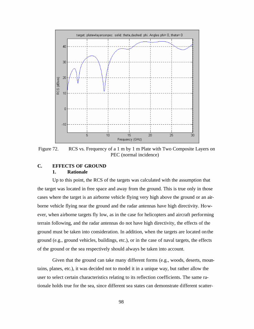
98

Figure 72. RCS vs. Frequency of a 1 m by 1 m Plate with Two Composite Layers on

PEC (normal incidence)

C. EFFECTS OF GROUND 1. Rationale

Up to this point, the RCS of the targets was calculated with the assumption that

the target was located in free space and away from the ground. This is true only in those

cases where the target is an airborne vehicle flying very high above the ground or an air-

borne vehicle flying near the ground and the radar antennas have high directivity. How-

ever, when airborne targets fly low, as in the case for helicopters and aircraft performing

terrain following, and the radar antennas do not have high directivity, the effects of the

ground must be taken into consideration. In addition, when the targets are located on the

ground (e.g., ground vehicles, buildings, etc.), or in the case of naval targets, the effects

of the ground or the sea respectively should always be taken into account.

Given that the ground can take many different forms (e.g., woods, deserts, moun-

tains, planes, etc.), it was decided not to model it in a unique way, but rather allow the

user to select certain characteristics relating to its reflection coefficients. The same ra-

tionale holds true for the sea, since different sea states can demonstrate different scatter-

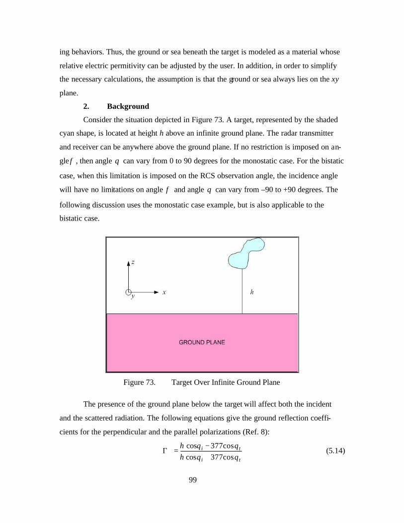
99

ing behaviors. Thus, the ground or sea beneath the target is modeled as a material whose

relative electric permitivity can be adjusted by the user. In addition, in order to simplify

the necessary calculations, the assumption is that the ground or sea always lies on the xy

plane.

2. Background

Consider the situation depicted in Figure 73. A target, represented by the shaded

cyan shape, is located at height h above an infinite ground plane. The radar transmitter

and receiver can be anywhere above the ground plane. If no restriction is imposed on an-

gleφ , then angle θ can vary from 0 to 90 degrees for the monostatic case. For the bistatic

case, when this limitation is imposed on the RCS observation angle, the incidence angle

will have no limitations on angle φ and angle θ can vary from –90 to +90 degrees. The

following discussion uses the monostatic case example, but is also applicable to the

bistatic case.

Figure 73. Target Over Infinite Ground Plane

The presence of the ground plane below the target will affect both the incident

and the scattered radiation. The following equations give the ground reflection coeffi-

cients for the perpendicular and the parallel polarizations (Ref. 8):

cos 377coscos 377cos

i t

i t

η θ θη θ θ⊥

−Γ =

+ (5.14)

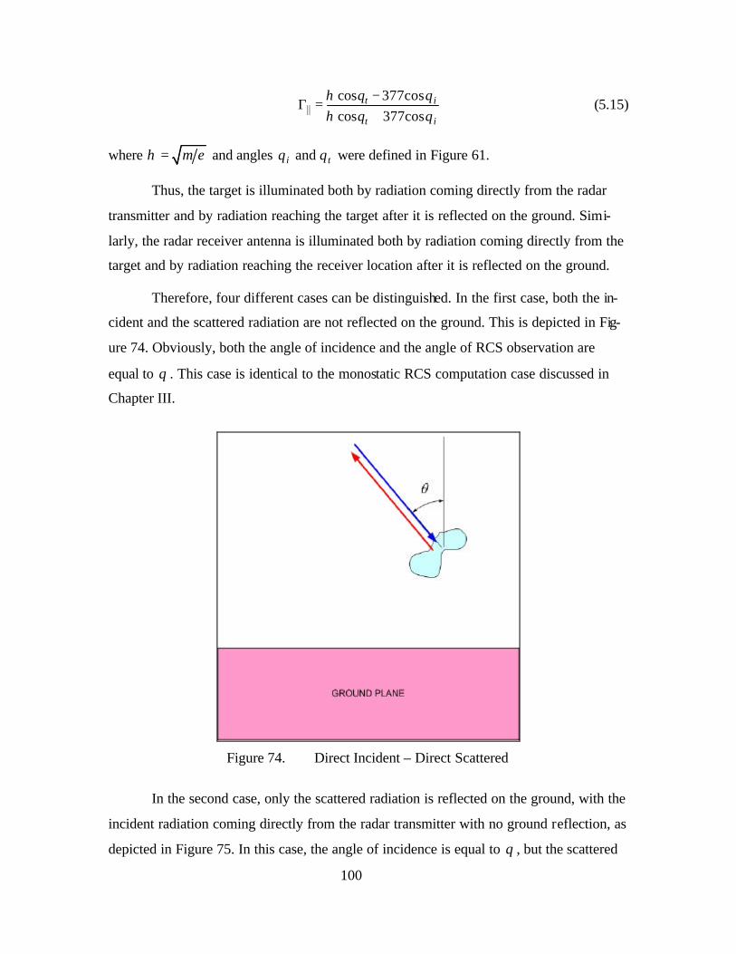
100

cos 377coscos 377cos

t i

t i

η θ θη θ θ

−Γ =

+P (5.15)

where η µ ε= and angles and i tθ θ were defined in Figure 61.

Thus, the target is illuminated both by radiation coming directly from the radar

transmitter and by radiation reaching the target after it is reflected on the ground. Simi-

larly, the radar receiver antenna is illuminated both by radiation coming directly from the

target and by radiation reaching the receiver location after it is reflected on the ground.

Therefore, four different cases can be distinguished. In the first case, both the in-

cident and the scattered radiation are not reflected on the ground. This is depicted in Fig-

ure 74. Obviously, both the angle of incidence and the angle of RCS observation are

equal to θ . This case is identical to the monostatic RCS computation case discussed in

Chapter III.

Figure 74. Direct Incident – Direct Scattered

In the second case, only the scattered radiation is reflected on the ground, with the

incident radiation coming directly from the radar transmitter with no ground reflection, as

depicted in Figure 75. In this case, the angle of incidence is equal to θ , but the scattered

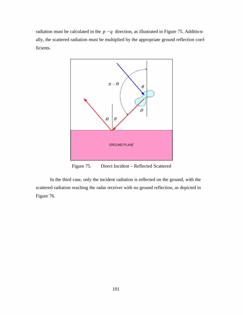
101

radiation must be calculated in the π θ− direction, as illustrated in Figure 75. Addition-

ally, the scattered radiation must be multiplied by the appropriate ground reflection coef-

ficients.

Figure 75. Direct Incident – Reflected Scattered

In the third case, only the incident radiation is reflected on the ground, with the

scattered radiation reaching the radar receiver with no ground reflection, as depicted in

Figure 76.

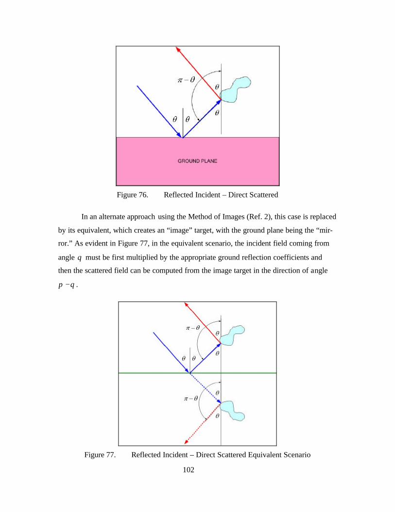
102

Figure 76. Reflected Incident – Direct Scattered

In an alternate approach using the Method of Images (Ref. 2), this case is replaced

by its equivalent, which creates an “image” target, with the ground plane being the “mir-

ror.” As evident in Figure 77, in the equivalent scenario, the incident field coming from

angle θ must be first multiplied by the appropriate ground reflection coefficients and

then the scattered field can be computed from the image target in the direction of angle

π θ− .

Figure 77. Reflected Incident – Direct Scattered Equivalent Scenario

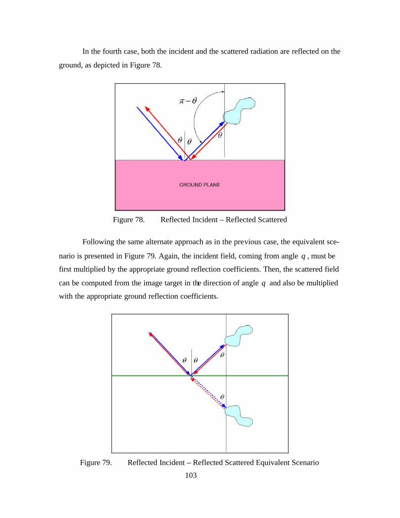
103

In the fourth case, both the incident and the scattered radiation are reflected on the

ground, as depicted in Figure 78.

Figure 78. Reflected Incident – Reflected Scattered

Following the same alternate approach as in the previous case, the equivalent sce-

nario is presented in Figure 79. Again, the incident field, coming from angle θ , must be

first multiplied by the appropriate ground reflection coefficients. Then, the scattered field

can be computed from the image target in the direction of angle θ and also be multiplied

with the appropriate ground reflection coefficients.

Figure 79. Reflected Incident – Reflected Scattered Equivalent Scenario

104

Summarizing, the following procedure can compute the approximate effects of

the ground on RCS:

a. A symmetric model is created relative to the xy plane.

b. For the incident radiation, the scattered radiation is computed from the original model at the θ angle (i.e., first case)

c. For the incident radiation, the scattered radiation is computed from the original model at the π θ− angle and multiplied by the ground reflection coefficients (i.e., second case)

d. The incident radiation is multiplied by the ground reflection coefficients. The scattered radiation is computed from the symmetric model at the π θ− angle (i.e., third case)

e. The incident radiation is multiplied by the ground reflection coefficients. The scattered radiation is computed from the symmetric model at the θ angle and multiplied by the ground reflection coefficients (i.e., fourth case)

f. The scattered radiation from steps b, c, d, and e is vector summed.

g. The RCS can be computed

3. Procedure

As previously discussed, the ground plane, when used, is always limited to the xy

plane, indicating that the model must be placed at the desired height over this plane. This

is accomplished by utilizing the Move button in the Graphical Model Design GUI, as de-

scribed in Section D of Chapter IV.

Once the target is placed at the desired height, the user can select whether to in-

clude the use of ground plane in the computations of monostatic or bistatic RCS versus

angle or versus frequency, or to perform RCS computations neglecting the ground. The

controls by which the user can make this selection are circled in Figure 80, which per-

tains to the calculation of monostatic RCS versus frequency. Similar controls appear in

the GUIs used for the other cases of RCS calculation.

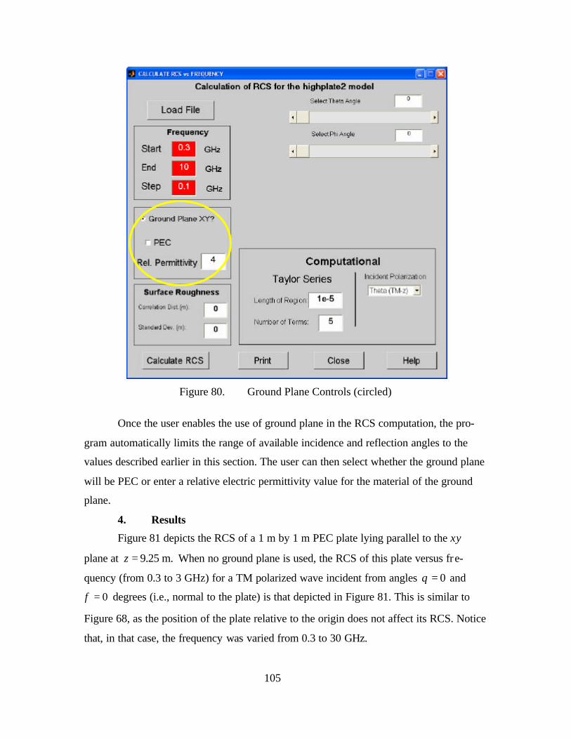
105

Figure 80. Ground Plane Controls (circled)

Once the user enables the use of ground plane in the RCS computation, the pro-

gram automatically limits the range of available incidence and reflection angles to the

values described earlier in this section. The user can then select whether the ground plane

will be PEC or enter a relative electric permittivity value for the material of the ground

plane.

4. Results

Figure 81 depicts the RCS of a 1 m by 1 m PEC plate lying parallel to the xy

plane at 9.25 m.z = When no ground plane is used, the RCS of this plate versus fre-

quency (from 0.3 to 3 GHz) for a TM polarized wave incident from angles 0θ = and

0φ = degrees (i.e., normal to the plate) is that depicted in Figure 81. This is similar to

Figure 68, as the position of the plate relative to the origin does not affect its RCS. Notice

that, in that case, the frequency was varied from 0.3 to 30 GHz.

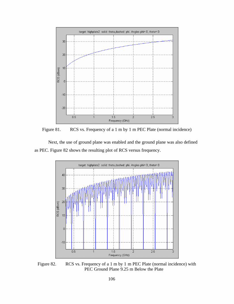
106

Figure 81. RCS vs. Frequency of a 1 m by 1 m PEC Plate (normal incidence)

Next, the use of ground plane was enabled and the ground plane was also defined

as PEC. Figure 82 shows the resulting plot of RCS versus frequency.

Figure 82. RCS vs. Frequency of a 1 m by 1 m PEC Plate (normal incidence) with

PEC Ground Plane 9.25 m Below the Plate

107

It is obvious that once again the maximum value of the RCS is increasing with the

square of frequency, following the pattern depicted in Figure 81. However, the vector

sum of the scattered fields from the four cases described previously (i.e., Direct Inc i-

dent/Direct Scattered, Direct Incident/Reflected Scattered, Reflected Incident /Direct

Scattered, and Reflected Incident /Reflected Scattered) has produced significant variations

in the RCS values.

Indeed, depending on the frequency of the incident wave, those four scattered

fields can have the same phase, resulting in constructive interference. Then, the total scat-

tered field is increased by a factor of four, which increases the total RCS by a factor of

16, since RCS is proportional to the square of the scattered field, as shown in Equation

(2.5). This corresponds to an increase of approximately 12 dBsm. Indeed, a comparison

of Figures 81 and 82 reveals that the difference in the highest RCS values at the same

frequency is approximately 12 dBsm.

For other frequency values, the four scattered fields might cancel each other, re-

sulting in zero total scattered field, which is represented by the nulls that appear in the

RCS plot in Figure 82. Moreover, for other frequencies, the vector sum of the four scat-

tered fields can produce RCS values higher or lower than those depicted in Figure 81.

These are represented by the variations of the RCS in Figure 82 between the maximum

values and the nulls.

D. SUMMARY

This concludes the description of the new computational capabilities added to the

POFACETS program. The theoretical background, the implementation and the results for

the exploitation of symmetry planes, the use of different materials and coatings on mod-

els, and the effects of the ground have been presented and discussed. The next and final

chapter summarizes the work of this thesis and suggests further potential improvements

to the program.

108


109

VI. SUMMARY AND RECOMMENDATIONS

A. SUMMARY

The objective of this thesis was to improve the existing POFACETS RCS predic-

tion software tool. This objective was achieved by providing new functionalities and add-

ing new computational capabilities to the POFACETS 2.3 version.

The new functionalities include the GUI and model database upgrade, the im-

provement of the manual model design options, the creation of a graphical model design

GUI, the inclusion of capabilities for importing and exporting models compatible with

commercial CAD programs, the inclusion of capabilities for a combination of existing

models, the computation of RCS versus frequency, and the creation of new options for

the display of RCS results.

The new computational capabilities include the exploitation of symmetry planes

in target models to decrease run-time for RCS prediction, the development of a user-

updateable database of materials which can be applied to models in one or multiple lay-

ers, the computation of the effects of materials and coatings in the model RCS, and the

approximate effect of the ground on the RCS of a model.

Overall, the program is now user-friendlier, by providing easy-to-use GUIs and

familiar controls, while minimizing the possibility for erroneous input. Moreover, the

creation of complex models was facilitated through the use of an automated standard

model design and the new capabilities, which allow the program to combine existing

models and share models with CAD software. Despite the new improvements and com-

putational capabilities, minimal effect occurred to the required program execution time,

while the option for the exploitation of symmetry planes, when these exist, can drastically

decrease execution time.

The versatility of the program was enhanced by allowing the capability for RCS

computation versus frequency and providing a broader range of options for RCS display.

Indeed, these capabilities allow the use of the program not only for RCS prediction, but

for RCS analysis as well.

110

Finally, the capability to use very complex models, the materials database, the ca-

pability to apply different types of materials and coatings to the models’ surfaces and the

inclusion of the effects of the ground on RCS, have made the POFACETS 3.0 a much

more useful tool regarding real-world RCS prediction and analysis problems.

B. RECOMMENDATIONS

The POFACETS 3.0 program is implemented in the current version of the

MATLAB software. Thus, it can be easily modified and upgraded through the wide vari-

ety of tools that this software package provides. There are two areas of potential im-

provements that could further enhance the value and usefulness of the POFACETS pro-

gram.

The first area pertains to the enhancement of the capabilities for importing models

from other CAD software. Other commercia l CAD or RCS prediction software packages

can be considered as candidates for importing models. In addition, the capability to im-

port AUTOCAD standard files, and not just text stereo- lithographic format, would be a

significant addition to the features of the program.

The second area pertains to the limitations in the RCS prediction, which are in-

herent to the Physical Optics method. As previously discussed, certain significant scatter-

ing mechanisms, such as second reflections, diffraction, and traveling waves are not in-

cluded in the calculations. These mechanisms, of course, would have a significant effect

on program execution time, especially on large, complex models. Thus, it would be pos-

sible to implement them in the program as options, allowing the user to decide which of

these mechanisms to enable, depending on model complexity and the desired accuracy of

results.

111

APPENDIX. POFACETS FILES AND MODEL DATABASE STRUCTURE

The purpose of this Appendix is to provide basic information regarding the

framework of the POFACETS 3.0 program and the structure of its data files. This was

necessary, since the new functionalities and computational capabilities added to

POFACETS resulted in a complex program, consisting of 39 MATLAB script files and

16 MATLAB figure files. The following information provided aims mainly to help the

reader understand how the program operates, rather than serve as a user manual, since the

program itself incorporates detailed user instructions either through dialog boxes or

through help screens.

The Appendix consists of three parts. The first part presents the general frame-

work of the program, providing information about the interconnections between the vari-

ous script and figure files. The second part contains an alphabetical list of the script and

figure files comprising POFACETS 3.0, along with a brief description of the functions

performed by each file. The third part contains the description of the data structures in the

model database files and in the materials database file.

A. POFACETS FILE FRAMEWORK

The complete file framework of POFACETS 3.0 is presented in graphical form in

Figures 83 through 89. Each script file is represented by a cyan box, which contains the

name of the file. Each figure file is represented by a yellow box, which also contains the

name of the file. When a script and a figure file with the same name are attached, this

means that they comprise a pair of files which implements a GUI form. For each file or

pair of files, a brief description of its functionality is provided.

Execution flows from the top to bottom of the figures. Files are interconnected

through blue and red lines. Blue lines indicate that a script file is executed or a figure is

activated, as a result of an action in the higher–level file (e.g., a button is pressed). Red

lines indicate that one or more functions of the lower–level file are called from the

higher–level file.

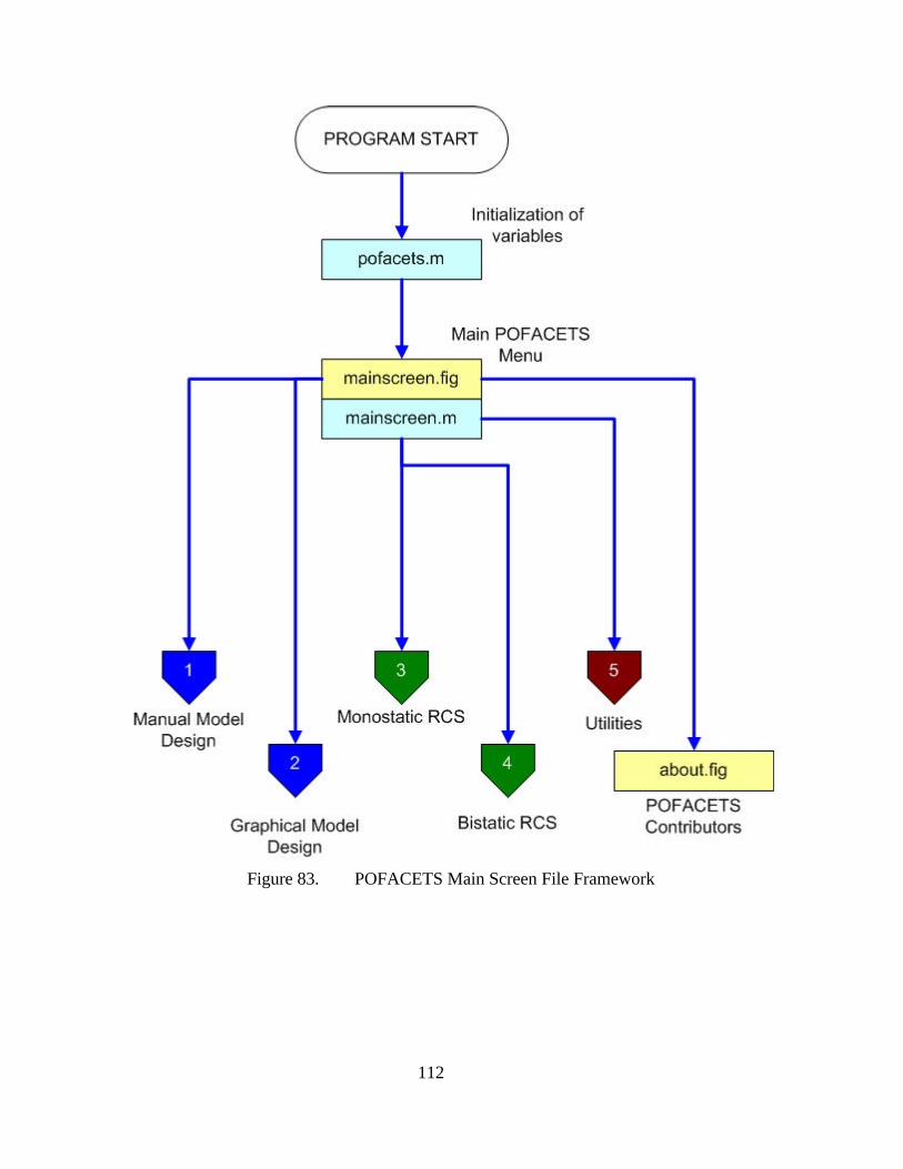
112

Figure 83. POFACETS Main Screen File Framework

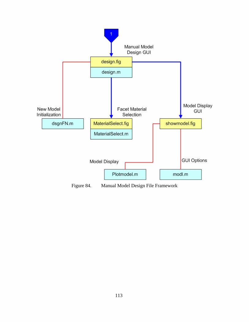
113

Figure 84. Manual Model Design File Framework

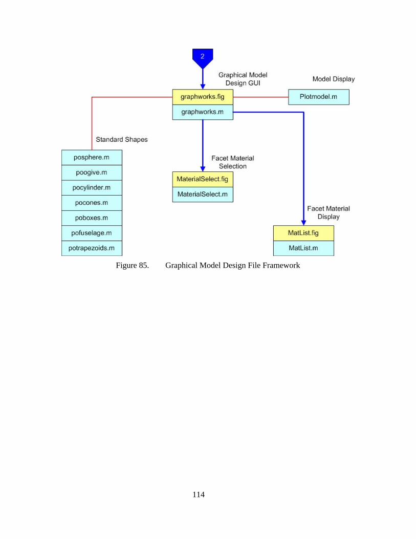
114

Figure 85. Graphical Model Design File Framework

115

Figure 86. Monostatic RCS Calculation File Framework

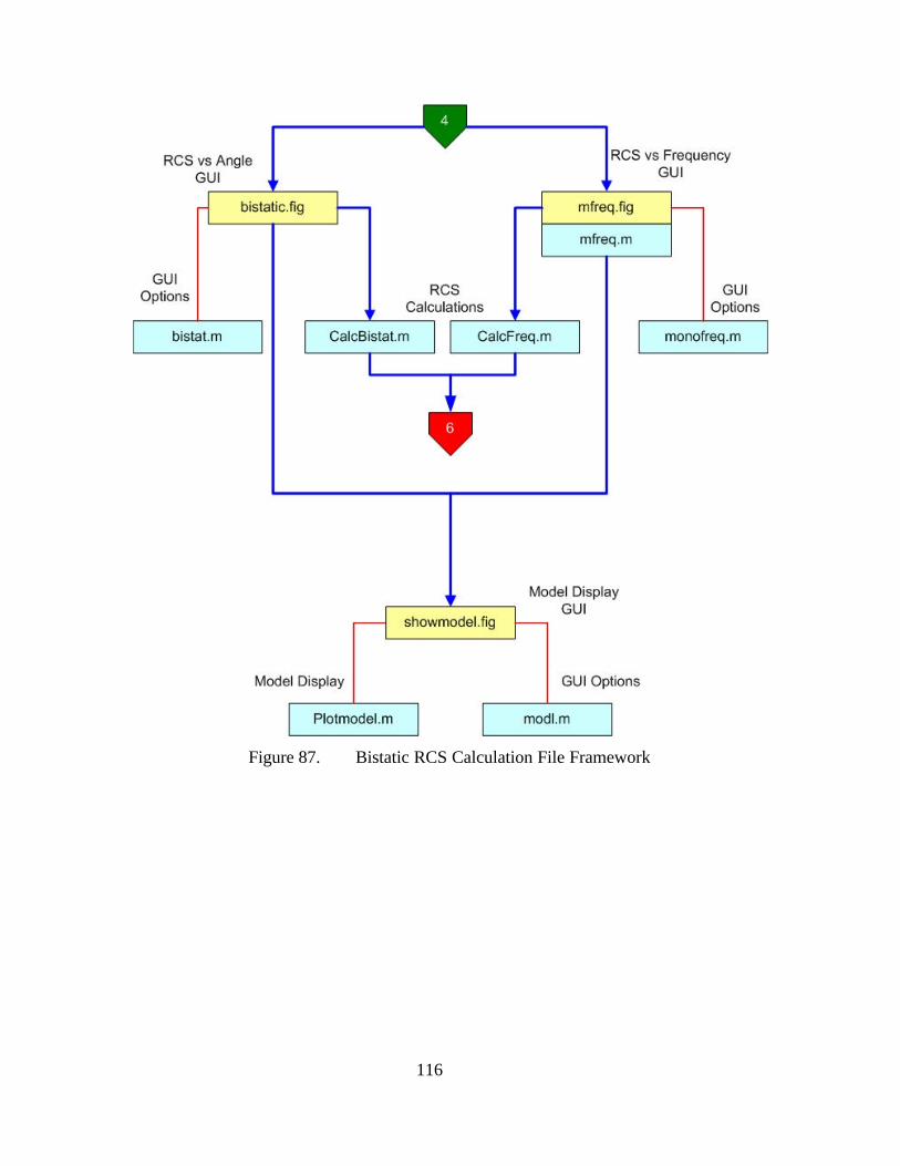
116

Figure 87. Bistatic RCS Calculation File Framework

117

Figure 88. Utilities File Framework

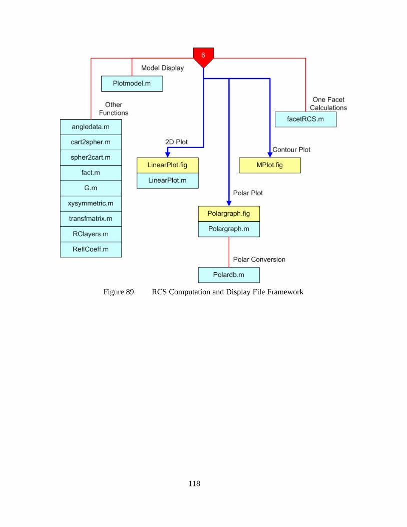
118

Figure 89. RCS Computation and Display File Framework

119

B. POFACETS FILE DESCRIPTION

The following list contains all the script and figure files used in the POFACETS

3.0 program. The help files are not included in this list.

about.fig: This file creates the GUI form that presents information about the con-

tributors to the POFACETS program

angledata.m: This function computes the direction cosines of an angle

bistat.m: This program implements the functionalities of the Bistatic RCS Calcu-

lation GUI

bistatic.fig: This file creates the Bistatic RCS Calculation GUI

CalcBistat.m: This file computes the bistatic RCS of a target model versus angle

CalcFreq.m: This file computes the monostatic or the bistatic RCS of a target

model versus frequency

CalcMono.m: This file computes the monostatic RCS of a target model versus an-

gle

cart2sphere.m: This function converts Cartesian coordinates to spherical coordi-

nates

design.fig & design.m: This pair of files creates the Manual Model Design GUI

dsgnFN.m: This file performs data initialization of variables for the manual crea-

tion of a new model

facetRCS.m: This function calculates the scattered and diffuse field from a single

facet for a given set of incident wave parameters

fact.m: This file implements the factorial function

G.m: This file implements the gamma function described in equations (3.47) and

(3.48)

graphworks.fig & graphworks.m: This pair of files creates the Graphical Model

Design GUI

hlpgui.fig: This file creates the GUI used to present help to the user

120

LinearPlot.fig & LinearPlot.m: This pair of files creates the GUI used to display

two–dimensional RCS graphs and select the dynamic range of these graphs

mainscreen.fig & mainscreen.m: This pair of files creates the GUI activated upon

program execution

MaterialDB.fig & MaterialDB.m: This pair of files creates the GUI used to edit

the materials database

materials.mat: This file contains the data of the materials database

MaterialSelect.fig & MaterialSelect.m: This pair of files creates the GUI that al-

lows the user to select different materials or layers of materials for the facets of a model

MatList.fig & MatList.m: This pair of files creates the GUI that allows the user to

view the materials or layers of materials of a model

mfreq.fig & mfreq.m: This pair of files creates the RCS Calculation versus Fre-

quency GUI for both the monostatic and the bistatic cases

modl.m: This file implements the functionalities of the GUI that displays a model

in the manual design case

mono.m: This file implements the functionalities of the Monostatic RCS Calcula-

tion GUI

monofreq.m: This file implements the functionalities of the RCS Calculation ver-

sus Frequency GUI for both the monostatic and the bistatic cases

monostatic.fig This creates the Monostatic RCS Calculation GUI

Mplot.fig: This file creates the GUI used for contour plots

Plotmodel.m: This file displays a model in either the manual or the graphical de-

sign case

poboxes.m: This file creates the model of a box

pocones.m: This file creates the model of a cone

pocylinder.m: This file creates the model of a cylinder

121

pofacets.m: This file must be executed to run POFACETS. It performs the initiali-

zation of variables and activates the program’s main screen

pofuselage.m: This file creates the model of a fuselage

Polardb.m: This file converts data so that they can be displayed in polar coordi-

nate form

Polargraph.fig & Polargraph.m: This pair of file creates the GUI used to present

the RCS plots in polar form

poogive.m: This file creates the model of an ogive

posphere.m: This file creates the model of a sphere or an ellipsoid

potrapezoids.m: This file creates the model of a trapezoid

Rclayers.m: This function calculates the reflection coefficients for layers of mate-

rials

ReflCoeff.m: This file creates the reflection coefficients from a surface for a given

angle of incidence

showmodel.fig: This file creates the GUI used for model display in the manual de-

sign case

spher2cart.m: This function converts spherical coordinates to Cartesian coordi-

nates

spherglobal2local.m: This function converts global spherical coordinates to local

facet spherical coordinates

spherlocal2global.m: This function converts local facet spherical coordinates to

global spherical coordinates

transfmatrix.m: This function calculates the transformation matrices of a facet

utilities.fig & utilities.m: This pair of file creates the Utilities GUI

xysymmetric.m: This function creates an “image” model, which is symmetric to

the original model relative to the ( , )x y plane

122

C. POFACETS DATA STRUCTURES DESCRIPTION

POFACETS uses two types of data files: the model files and the material database

file described below.

1. Model File Structure

Each model file is comprised of the following data structures.

a. Coord

This is a data array that contains the coordinates of the vertices of the

model. Each row corresponds to a vertex. The first field in each row represents the x co-

ordinate of the vertex, the second field represents y and the third represents z.

b. Facet

This is a data array that contains the definition data for the facets of the

model. Each row corresponds to a facet. The first three fields in each row represent the

facet’s vertices. The sequence of the vertices defines the normal to the facet according to

the right hand rule. The fourth field in each row indicates whether a facet can only be il-

luminated from its front side (when it contains a 1) or from both its back and front side

(when it contains a 0). The fifth field in each row is the surface resistivity of the facet

normalized to the impedance of free space (377 ohms).

c. Scale

This field stores the scale of the model

d. Symplanes

This is a data array that contains the points that form the symmetry planes

of the model. If no symmetry planes exist, the array simply holds one row with three

fields equal to zero. If symmetry planes exist, each symmetry plane is defined by three

points represented by three consecutive rows. Each row contains the coordinates ( , , )x y z

of each point. The sequence of the points defines the normal to the symmetry plane ac-

cording to the right hand rule. Up to three symmetry planes (i.e., nine rows) can be

stored.

e. Comments

This is a cell array that contains the description of the parts of the model to

which the facets belong. Each row contains the parts description for one facet.

123

f. Matrl

This is a cell array that contains the material of the facets of the model.

Each row of the cell array corresponds to one facet. The first cell of the array contains the

description of the type of the material used on the facet. The available options here are:

“PEC”, “Composite”, “Composite Layer on PEC”, “Multiple Layers”, and “Multiple

Layers on PEC”. The second cell is a one–row vector. For each layer of material used, 5

columns are included in the vector. Thus, if three layers are used, the vector will have 15

columns. In each layer, the first column is the relative electric permittivity, the second

column is the loss tangent, the third column is the real part of the relative magnetic per-

meability, the fourth column is the imaginary part of the relative magnetic permeability,

and the fifth column is the thickness of the layer in millimeters.

2. Material Database File Structure

The material database file contains a struct array called materials.mat, which is

comprised of the following fields.

a. Name

This field holds the name of the material.

b. er

This field holds the relative electric permittivity of the material.

c. tande

This field holds the loss tangent of the material.

d. mpr

This field holds the real part of the relative magnetic permeability of the

material.

e. m2pr

This field holds the imaginary part of the relative magnetic permeability of

the material.

124


125

LIST OF REFERENCES

1. Schleher, D. Curtis, Electronic Warfare in the Information Age, Artech House, Norwood, Massachusetts, 1999.

2. Jenn, David C., Radar and Laser Cross Section Engineering, AIAA Educations Series, Washington D.C., 1995.

3. Garrido, Elmo Jr., Graphical User Interface for a Physical Optics Radar Cross Section Prediction Code, Master’s Thesis, Naval Postgraduate School, Monterey, California, September 2000.

4. Skolnik, Merill I., Introduction to Radar Systems, 3rd Edition, McGraw Hill, New York, 2001.

5. Jenn, David C., Microwave Devices and Radar Lecture Notes, Version 4.7, Vol-ume I (unpublished).

6. Moreira, Fernando J. S., and Prata, Aluizio Jr., “A Self Predictor-Corrector Algo-rithm for Efficient Evaluation of Reflector Antenna Radiation Integrals,” IEEE Transactions on Antennas and Propagation, vol. 42, no. 2, pp. 246-254, February 1994.

7. Wadell, J. M., Scattering From Rough Surfaces, Master’s Thesis, Naval Post-graduate School, Monterey, California, September 1995.

8. Jenn, David C., Geometrical Optics and the Geometrical Theory of Diffraction Notes, Version 1.5, 2004 (unpublished).

9. Knott, E., Shaeffer, J., and Tuley, M., Radar Cross Section, 2nd Ed., Artech House, Norwood, Massachusetts, 1993.

10. Knott E., Shaeffer, J., and Tuley, M., Radar Cross Section: Its Prediction, Meas-urement and Reduction, Artech House, Norwood, Massachusetts, 1985.

11. Faros, N., Radar Cross Section Synthesis for Planar Resistive Surfaces, Master’s Thesis, Naval Postgraduate School, Monterey, California, December 1994.

12. Stutzman, W., and Thiele, G., Antenna Theory and Design, 2nd Ed,. Wiley, Hobo-ken, New Jersey, 1998.

13. Chapman, Stephen J., MATLAB Programming for Engineers, 2nd Ed., Brooks/Cole, Pacific Grove, California, 2002.

126


127

INITIAL DISTRIBUTION LIST

1. Defense Technical Information Center Ft. Belvoir, Virginia

2. Dudley Knox Library Naval Postgraduate School Monterey, California

3. David C. Jenn, Code EC/Jn Department of Electrical and Computer Engineering

Monterey, California

4. D. Curtis Schleher, Code IS/Sc Department of Information Sciences

Monterey, California 5. Phillip E. Pace, Code EC/Pc

Department of Electrical and Computer Engineering Monterey, California

6. Dan C. Boger, Code IS/Bo Department of Information Sciences Monterey, California

7. John P. Powers, Code EC/Po Department of Electrical and Computer Engineering Monterey, California

8. Filippos Chatzigeorgiadis Hellenic Air Force Athens, Greece

Documents

NAVAL POSTGRADUATE SCHOOLdtic.mil/dtic/tr/fulltext/u2/a427120.pdfNAVAL POSTGRADUATE SCHOOL September 2004 ... Advantage of Stealth Fighter over Conventional Fighter ... Polar Plot