NAVAL POSTGRADUATE SCHOOLdtic.mil/dtic/tr/fulltext/u2/a128974.pdf · NAVAL POSTGRADUATE SCHOOL Monterey, California iM-DTIC I1ELECTE i1 THESIS D GUIDE FOR CONCEPTUAL HELICOPTER DESIGN

NAVAL POSTGRADUATE SCHOOLMonterey, California

iM

- DTICI1ELECTE i1

THESIS D

GUIDE FOR CONCEPTUALHELICOPTER DESIGN

by

Stephen Glenn Kee

June 1983

Thesis Advisor: Donald M. Layton

(LJ Approved for public release; distribution unlimited...

j 06 06 020

zAm

SSCUmATV CtLAWIFIC&?TU OW TWIS PaGR M4111 DOIN 8066"

ESAD wpuryiCW(nrsUOWF DOOJAMATM N WJrn: COktPLT!NG FOR

~-VNP"WTmuu 11UNWNVT AccaCUISme: a NII NI SCATALOG IuU41iN

4. T11161 (ied 211111,0b19 a. TYPZ Do 1119ONT A Pfff0h co vieao

Guid fo Coceptal eliopte Deign Master's ThesisGuid fo Coceptal eliopte Deign June 1983

6. 090OODINwOnom. "SPIOT kulMUlef

?.~~~~~~~ AGIM3a)S OTUC AANT WMpgIrgA

Stephen Glenn Kee

*. TI O NI -*g uo u ss o aNIZAT O N Ns a E AND LO OSE M AMR* 9%9 111 r* Ofit.PA jS . T-AISAAA 6 WORK UNIT 144.111119

Naval Postgraduate SchoolMonterey, California 93940

11. CO14WULING OPPIC9 IIIAIR AN* ASGOESS it. BEPaRT SATE

Naval Postgraduate School June 1983Monterey, California 93940 122~' GE

'a w-U6*TORI1-WAagECY NoAaE & AQOOSESWiS &MS.It t C411018IiNS 0t0b.) 1S. SECURITV CLASS. (00io pe I~,

IS.. WC SIFICATIO/ OWNGIA ING

r. 7MVIG~ut@Ul ITArgtaul NW fi t.Upe")

Approved for public release; distribution unlimited.

17. OISTRUUTION STATNUCUT (Of 0 8601110 000"ift Olee M f is fbun - Re')

SSUPPLaMENTARY 0OTEts

10IR. *EY ORD (COmaums - -Ol ads it nesoonV OW #~Or or wool Wia

Helicopter DesignDesign Education

AOTRACT (CAMI... seine.tU1s oldi ein "a -o""4 0401144 &W a sun*@"

1A conceptual helicopter design method utilizing closed formformulas and approximations from historical data is developedfor use in a helicopter design course. The design manualis to be used for the conceptual design of a single mainrotor, utility helicopter. The manual was written principallyfor use in AE4306--Helicopter Design.,

140 , u avolw of I NOV 060 ems us.f

MI

Approved for public release; distribution unlimited.

Guide for Conceptual Helicopter Design

by

Stephen Glenn KeeCaptain, United States Army

B.S., United States Military Academy, 1973

Submitted in partial fulfillment of the

requirements for the degree of

MASTER OF SCIENCE IN AERONAUTICAL ENGINEERING

from the

NAVAL POSTGRADUATE SCHOOLJune 1983

Author:

Approved by: ,-/Th sis Advisor

AOccssion For 1

NTIS GRAV n-- irman, Dtpartmif of AeronauticsDTIC TAR~ 11UnannouncedJust 4'Dean'of Science and EngineeringDistribiuton/.

Availability Codes 90:6 2Avail and/or -- ow 2

Dist Special

T -

ABSTRACT

A conceptual helicopter design method utilizing closed

form formulas and approximations from historical data is

developed for use in a helicopter design course. The design

manual is to be used for the conceptual design of a single

main rotor, utility helicopter. The manual was written

principally for use in AE4306--Helicopter Design.

3

.4-,

TABLE OF CONTENTS

I . INTRODUCTION . . . . . . . . . . . . . .. .. .... 5

A.* BACKGROUND . . . . . . . . . . . . . . . . . . 5

B. GOALS . . . . . . . . . . . . . . . . . . . . 6

II. APPROACH TO THE PROBLEM . .. . ... .. .. .. 7

III. THE SOLUTION . . . . o . . . . . . . . . . . . . . 9

IV. RESULTS . . . . . . . . . . . . . . . . . . . 11

V. CONCLUSIONS AND RECOMMENDATIONS . . . . . . . . . 12

LIST OF REFERENCES . . .. .. .. .. .... .. .... 13

APPENDIX A: HELICOPTER DESIGN MANUAL . . . . . . .* . 14

APPENDIX B: HELICOPTER DESIGN COURSE HANDOUTS . . . . 71

APPENDIX C: EXAM8PLE OF CONCEPTUAL HELICOPTER DESIGN **84

INITIAL DISTRIBUTION LIST ............ . ... .. 122

4

.4

I. INTRODUCTION

A. BACKGROUND

The methods of conceptual helicopter design have changed

dramatically over the past 30 years. Two principal reasons

for this change are the greatly increased research and

development costs and the scientific advances which have led

to engineering specialization. Today almost all new produc-

tion helicopters are to a great extent hybrids of their

predecessors, with technological advances applied to

existing systems rather than to an entirely new design. The

helicopters of today are designed by committees composed of

specialists in various fields who compromise and optimize to

reach a final design. As a result the designer of today is

presented with challenges not faced by his predecessors.

Traditionally, design courses have been used to equip

the engineering student with the skills needed to meet the

challenges in the real world of engineering [Ref. 1]. Even

though the required skills have changed, design courses are

still very important in the education process; however,

design is no longer being taught in many aeronautical engi-

neering schools [Ref. 2]. In the field of helicopter design

this is due largely to the complexity of the subject matter.

When it was decided to incorporate a helicopter design

course into the curriculum at the Naval Postgraduate School,

5

the search for a design methodology that could be used in

this course led to the discovery that few texts on the heli-

copter design process exist. Many manufacturers have their

own methods, but since they rely so heavily on previous

in-house designs, they are not suitable for use in an educa-

tional framework. It became apparent that a conceptual

design process for the course would have to be developed.

B. GOALS

The goals of this study were to:

1. provide a simple design process for use in a capstonehelicopter design course,

2. provide an opportunity to exercise the skills ofoptimization and decision-making, aot only inengineering but in managerial areas as well, and

3. provide a framework from which further research canbe undertaken.

4

6

47!

II. APPROACH TO THE PROBLEM

The first step in the development of the helicopter

design course was to analyze the complex nature of heli-

copter engineering and to simplify its concepts into a

series of design steps. It became evident that the design

methodology would require an iterative process due to the

relationships among the major design variables. A decision

was made not to use the computer directly to perform the

iterations, so that the student, as he performed the

required calculations, would develop a much greater under-

standing of the interrelationships of the variables.

However, the decision not to utilize a computer increases

the complexity and length of the process.

It was decided to use a guided design technique of

instruction, in order to limit the time and complexity

factors.

"Guided design is a relatively recent innovation inwhich students are first presented with a problemsetting. Sequential written instructions . . . arethen used to expose them to desired course materialand to aid them in learning to use rational problemsolving techniques. The guidance feature makes theapproach best suited to elementary courses or forintroductory projects in an advanced course." (Ref. 3]

Another advantage of the guided design process is that it

frees the student from lecture sessions and allows the

instructor to focus on critical areas. A disadvantage of

7

77

this structure is that student creativity and initiative is

somewhat inhibited.

The second step was to incorporate the design method-

ology into a structure which would guide the student to a

completed project and allow for creativity and initiative.

8

III. THE SOLUTION

The design process uses closed form equations to provide

a numerical analysis of helicopter theory. Where theory

does not provide an exact solution, historical trends are

used to approximate. The historical data that is obtained

for use in the design process should reflect the type of

helicopter that is to be designed. Specifications and

mission requirements must be provided by the instructor.

The design process was incorporated into a design manual

(Appendix A) for student use. Included in Appendix B are

sample handouts which provide the specifications and histor-

ical data necessary to use this manual. These handouts

limit the design to a single rotor, utility helicopter. The

difficulty of the design process can be adjusted by varying

the amount of information provided or the type of helicopter

to be designed can be changed through modification of these

handouts. Additionally, the handouts provide a means by

which the course can be improved by continued research

without the requirement of having to rewrite or modify the

manual.

The student is expected to have a basic understanding of

the theory of helicopter performance. Many of the equations

used in the manual were taken from Helicopter Performance

..! " ,ii9* I:

[Ref. 4]. Those areas of theory that are not included in

Reference 4 were covered in greater detail in the manuAl.

During the design process the student is required to

make decisions and optimize several factors. It was decided

to require the student to write several brief discussions at

these steps in the design process so that the instructor can

follow the student's reasoning in the critical decisions.

These discussions allow the student an opportunity to

exhibit initiative and creativity.

Several hand-held calculator programs [Ref. 5] and a

computer plotting routine (Ref. 6] have been developed for

use in the design process. These programs are mentioned in

the design manual where they are applicable. They have

been included to reduce the tedium of several repetitive

calculations.

An introduction to cost estimating relationships have

been included to broaden the student's perspective of real

world considerations and to allow the use of some managerial

skills.

10

IV. RESULTS

The design process has been included in a design manual

(See Appendix A) which is suitable for use in a helicopter

design course.

An example design is included in Appendix C. The speci-

fications and historical data used in this example are

included in Appendix B. The specifications for two addi-

tional designs are also contained in Appendix B (See HD-I).

C

!1

V. CONCLUSIONS AND RECOMMENDATIONS

The simplification of the field of helicopter engi-

neering into the design process presented in Appendix A

necessitated that some areas be slighted. Several major

areas are either covered only superficially or omitted due

to the time constraint that the student would face in a one

quarter design course. Typical of these areas are airframe

design, structural designs, cost, tail rotor and vertical

fin effects, and power required to overcome retreating blade

stall effects. Other areas which were included must use

estimations or historical trends to reach a design due to a

lack of an adequate theory to predict real world data. The

weight estimating relationships and profile drag computa-

tions are examples. Future research in these areas could be

included in the design manual or the handouts.

Many of the decisions that the student is required to

make using the design process are based on a numerical anal-

ysis of the various factors. In the real world, many other

factors may be present which would necessitate a different

decision, so that in this sense the process is not a valid

representation. However, the design process as found in the

design manual should be useful as an educational tool.

12

4'" __-___,_____.. . . ._"_"____________-_______.... .. __-___.. . .. .. .....

LIST OF REFERENCES

1. Haupt, Urich, Needs and Challenges in Education forAircraft Design, p. F-I, Naval Postgraduate School,1973.

2. Ibid., p. 4.

3. Alic, J. A., "Integrating the Teaching of Design andMaterials", Engineering Education, Vol. 65, No. 7, pp.725-729, April 1975.

4. Layton, Donald M., Helicopter Performance, NavalPostgraduate School, 1980.

5. Fardink, Paul J., Hand-Held Computer Programs for Pre-liminary Helicopter Design, M.S. Thesis, Naval Post-graduate School, 1982.

6. Sullivan, Patrick, Helicopter Power ComputationPackage, Term Paper for AE4900, Naval PostgraduateSchool, 1982.

I

413

*'4

APPENDIX A

Helicopter Design Manual

by

CPT Stephen G. Kee

AE4306Professor Donald M. Layton

Department of AeronauticsNaval Postgraduate School

Monterey, California

June 1983

114

At .. ..

ABSTRACT

This design manual is to be used for the conceptual

design of a single main rotor, utility helicopter. The

design method utilizes closed form formulas and approxi-

mations from historical data. This manual was written

for use in AE4306--Helicopter Design.

15

CONTENTS

ABSTRACT . . . . . . . . . . . . . . . . . . . 15

Chapter page

1. INTRODUCTION . . . . . . . . . . . . . . . . . . . . .21

DESIGN OBJECTIVE .......... . . . . . . .21DESIGN PHASES . . ................ .23PROCEDURE ........................... . . .24APPLICABILITY . . . . .............. 25ASSUMPTIONS . . . . . ............ .25

2. MAIN ROTOR DESIGN ....... .................. 26

MAKE A ROUGH ESTIMATE OF THE MANUFACTURER'S EMPTYWEIGHT . . . . ........... ........ 26MAKE A ROUGH ESTIMATE OF GROSS WEIGHT .. ....... .. 26CALCULATE THE MAXIMUM TIP VELOCITY ......... 26DETERMINE THE ROTOR RADIUS ..... ............ ..26DETERMINE A FIRST-CUT ROTATIONAL VELOCITY ... . 27MAKE A FIRST-CUT DETERMINATION OF THRUSTCOEFFICIENT ...... ..... ....... .. . . . 27DETERMINE THE BLADE SOLIDITY.. .27DETERMINE THE NUMBER OF MAIN ROTOR BLADES*TO BE"USED ............. 28DETERMINE THE CHORD AND TE" ASPECT .ATIO. ....... .. 29DETERMINE THE AVERAGE LIFT COEFFICIENT . .... .30CHOOSE AN AIRFOIL SECTION FOR THE MAIN ROTORBLADES .................... 30DETERMINE AVERAGE LIFT CURVE SLOPE AND AVERAGEPROFILE DRAG COEFFICIENT ..... .............. .31

3. PRELIMINARY POWER CALCULATIONS ..... ............ 32

MAKE FIRST ESTIMATE OF THE POWER REQUIRED TOHOVER . . .................... .. 32MAKE SECOND GROSS WEIGHT ESTIMATE .. .... .. 32ESTABLISH FIGURE OF MERIT AT APPROXIMATELY 0.75* . .33REFINE SECOND GROSS WEIGHT ESTIMATE . ...... 34MAKE THIRD ESTIMATE OF POWER REQUIRED TO HOVER . . .35REPEAT THE GROSS WEIGHT ESTIMATE AND THE HOVERPOWER REQUIRED ITERATION.. . . . . 35DETERMINE THE POWER REQUIRED TO HOVER IGE, SSL . . .35

16

.................................j.*

DETERMINE THE PARASITE POWER REQUIRED IN FORWARDFLIGHT . ......... 35DETERMINE MAIN ROTOR POWER REQUIRED*AND'THE'MACHNUMBER OF THE ADVANCING BLADE TIP FOR FORWARDFLIGHT . . . . . . . . . . . . . . . ........ 36

4. TAIL ROTOR DESIGN . . . . . . . ............. 38

MAKE PRELIMINARY DETERMINATIONS OF TAIL ROTORGEOMETRY . . . . . . . . 38DETERMINE TAIL ROTOR POWER REQUiRED'AT HOVER OGE,SSL ...... 38DETERMINE TAIL ROTOR POWER REQUiRED'AND'TIP*MACH

EFFECTS FOR FORWARD FLIGHT ..... ............. .39

5. POWER CALCULATION REFINEMENTS ............ 41

DETERMINE TOTAL POWER REQUIRED FOR HOVER ANDFORWARD FLIGHT .................. 41DETERMINE COMPRESSIBILITY CORRECTION. . .42DETERMINE THE REQUIRED RSHP AT MAXIMUM VELOCITY . .43DETERMINE THE REQUIRED RSHP FOR HOVER (IGE) AT THESPECIFIED CEILING ................... 43DETERMINE THE TOTAL ESHP REQUIRED ... ......... 44

6. ENGINE SELECTION ........ ................... 45

SELECT TYPE AND NUMBER OF ENGINES - e . .... .45REVISE GROSS WEIGHT AND POWER REQUIRED-. ........ .48DETERMINE FUEL FLOW RATES AT VARIOUS POWERSETTINGS .......... ...................... 48

7. RANGE AND ENDURANCE CALCULATIONS ..... .......... 50

DETERMINE THE SLOPE OF THE FUEL FLOW VERSUS SHPLINE AND THE ZERO HORSEPOWER INTERCEPT ......... .50COMPUTE THE ZERO HORSEPOWER INTERCEPT ATSPECIFICATION CONDITIONS ....... ............ .51DETERMINE THE ZERO HORSEPOWER INCREMENT . . . . . .51DETERMINE THE MAXIMUM RANGE VELOCITY... . . . e.52DETERMINE THE MAXIMUM ENDURANCE VELOCITY AND THEREQUIRED FUEL FLOW RATE AT THIS VELOCITY . . . . . .53DETERMINE THE POWER REQUIRED AT SPECIFICATIONCRUISE VELOCITY AND THE REQUIRED FUEL FLOWRATE AT THIS VELOCITY . ......... . .. . .54DETERMINE THE TOTAL FUEL REQUIREMENTS FORSPECIFIED MAXIMUM RANGE ............ 54

8. MISCELLANEOUS CALCULATIONS . . . . . . . . . . . . . .56

COMPUTE DESIGN GROSS AND EMPTY WEIGHT . . . . . . .56DETERMINE RETREATING BLADE STALL VELOCITY . . . . .56

17

.. .. . aim .,.

DETERMINE BEST RATE OF CLIMB . . . . . . . . . . . .58COMPUTE MAXIMUM HOVER ALTITUDE (IGE) . . . . . . . .60COMPUTE SERVICE CEILING . . . . . . . . . . . . . .61

9.* FINAL CHECK . . . . . . . . . . . . . *.. .. .. . .62

MAKE FINAL CHECK FOR COMPLIANCE WITHSPECIFICATIONS . . . . . . . . . . .. .. .. .. .. 62

Appendix

A-i LIST OF HELICOPTER DESIGN COURSE HANDOUTS . . . . . .63

A-2 LIST OF SYMBOLS . . . . . . . . . . . . . . . . . . .64

A-3 SAMPLE FINAL SUMMARY FORMAT. ....... . . . . .*67

LIST OF REFERENCES . . . . . .. .. .. .. .. .. .. .. 69

BIBLIOGRAPHY . .. ...... ... .... .. ... .. 70

18

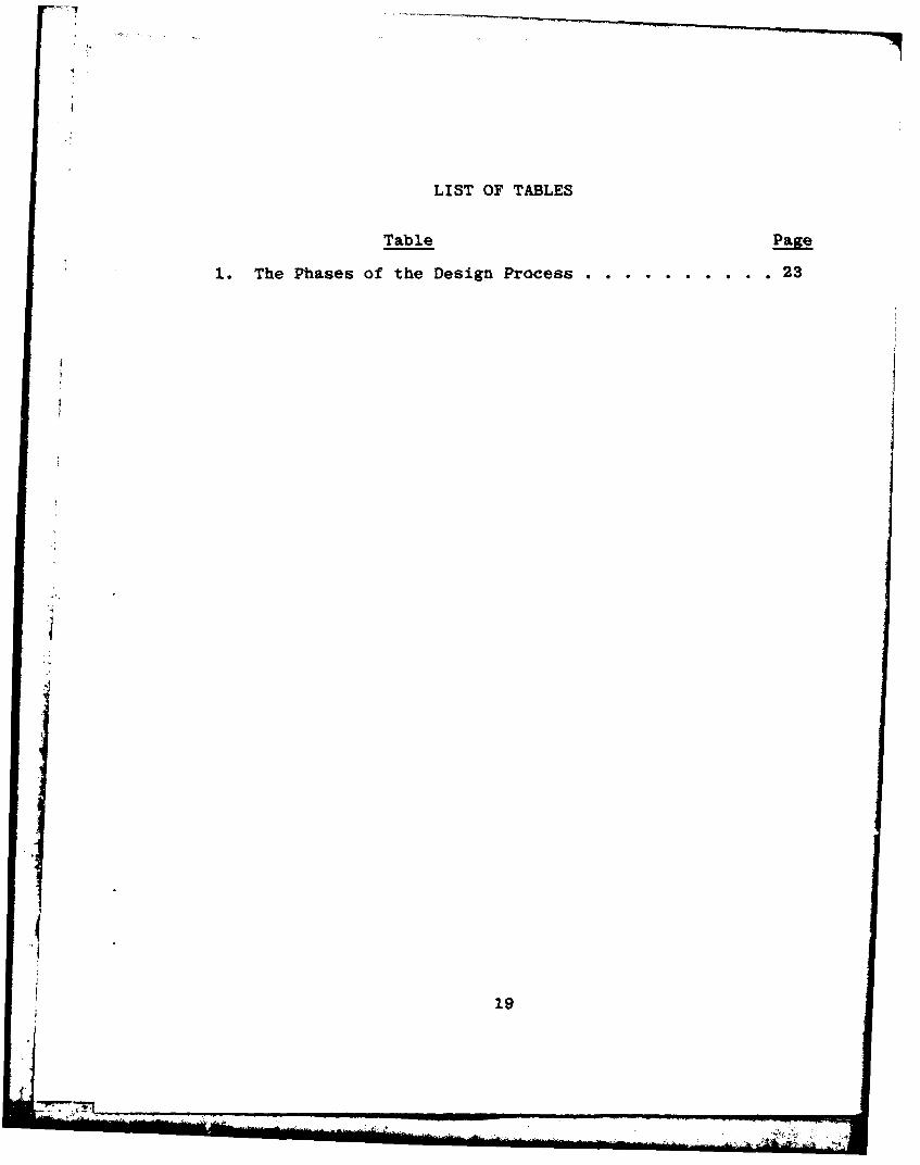
LIST OF TABLES

Table Rae

1.The Phases of the Design Process . . . . . . . . . . 23

19

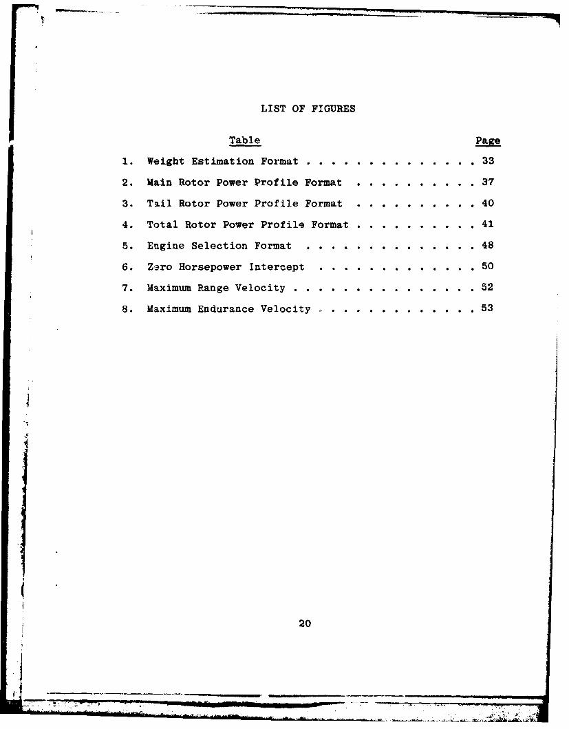
LIST OF FIGURES

Table Page

1. Weight Estimation Format ...... . . . . . . . 33

2. Main Rotor Power Profile Format . .... . . . . 37

3. Tail Rotor Power Profile Format . .... . . . . 40

4. Total Rotor Power Profile Format . .... . . . . 41

5. Engine Selection Format .. .. .. .. .. . . . 48

6. Zero Horsepower Intercept .. ........ . . . 50

7. Maximum Range Velocity . .. .. .. .. .. . . . 52

8. Maximum Endurance Velocity .. ............ 53

20

7 ! 7______ ___________

Chapter 1

INTRODUCTION

1.1 DESIGN OBJECTIVE

The goal of the design process is to optimize the mission

effectiveness of the design item. There are two groups of

factors which determine an item's mission effectiveness.

A) Operational factors.

1. Mission readiness which is a measure of the degree

to which an item is operable at the start of a

randomly selected mission. Mission readiness is

measured by an item's availability, reliability,

and maintainability.

a) Avaiiability is a function of the mean time

between maintenance actions and the maintenance

down time.

b) Reliability is a function of an item's failure

rate.

c) Maintainability is measured by the item's mean

time to repair.

2. Survivability which is a measure of the item's

ability to withstand a hostile man-made

environment and still be mission ready.

3. Overall performance which is a measure of how well

an item performs its designated mission.

21

.

B) Economic factors. The principle economic factor is

cost, which is a measure in dollars of the amount

required to design, produce, test, and operate an

item during its life-cycle.

One cost concept generally used to select among competing

designs is life-cycle cost, which is the sum of all expen-

ditures required from design conception to operational

phase-out. The life-cycle cost is comprised of research and

development costs, initial investment, annual operating

costs, annual maintenance costs, and salvage value. There

are two major difficulties in using the life-cycle cost

method of economic analysis. First, the task of assembling

sufficient historical data on similar systems to create

meaningful cost estimating relationships is quite large.

Second, the various parties involved in the procurement

process have a different perspective from that of the

designer. For example, a manufacturer may be more concerned

with an item's initial cost than with the user's maintenance

costs.

Any economic analysis of a design process should contain

the following elements:

A) a statement of the design objective and the effec-

tiveness measures which will be used to determine

if the objective is reached,

B) specification of the design choices (alternatives),

C) costs associated with each choice,

22

D) a set of relationships (a model) that relates each

choice to the effectiveness measures, and

E) the criteria or criterion which will be used to select

one of the design alternatives.

There are two major sources of uncertainty in any cost

analysis: inadequate or inaccurate specification of the

system being analyzed, and statistical inaccuracies in the

cost estimating relationships.

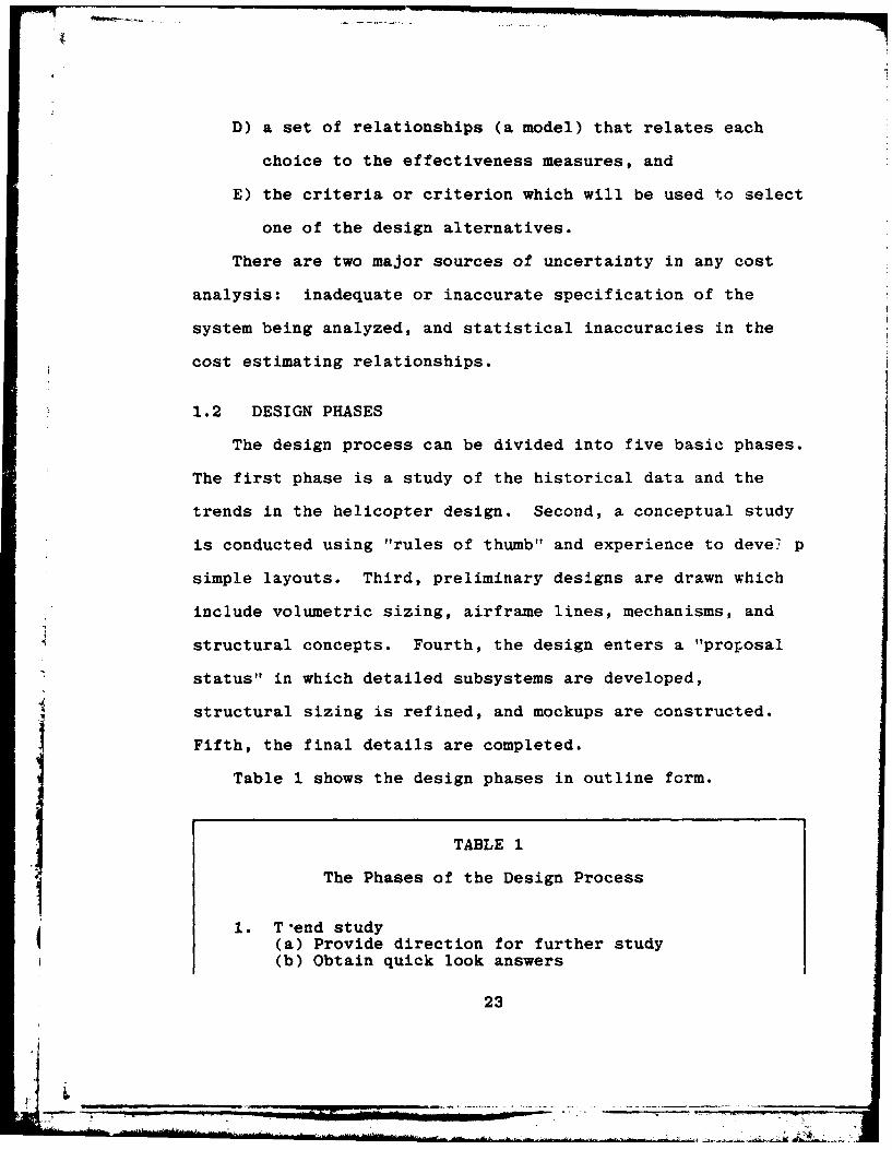
1.2 DESIGN PHASES

The design process can be divided into five basic phases.

The first phase is a study of the historical data and the

trends in the helicopter design. Second, a conceptual study

is conducted using "rules of thumb" and experience to devel p

simple layouts. Third, preliminary designs are drawn which

include volumetric sizing, airframe lines, mechanisms, and

structural concepts. Fourth, the design enters a "pror~osal

status" in which detailed subsystems are developed,

structural sizing is refined, and mockups are constructed.

Fifth, the final details are completed.

Table 1 shows the design phases in outline form.

TABLE 1

The Phases of the Design Process

1. T'end study(a) Provide direction for further study(b) Obtain quick look answers

23

2. Conceptual study(a) Compare configuration(b) Estimate size and cost(c) Establish feasibility(d) Recommend follow-on

3. Preliminary design(s.) Insure design practicality(b) Develop structural concepts(c) Develop concepts for mechanisms(d) Expand data base

4. "Proposal status" design(a) Increase detail of structure, weight, etc.(b) Increased confidence by risk reduction(c.) Support proposal commitment

5. Details

1.3 PROCEDURE

A design sequence has been delineated in a step-by-step

manner in the subsequent chapters of this manual. Each step

is numbered sequentially within each chapter so that ready

reference can be made to any step, when necessary, in other

chapters. Where calculations are required in the design

sequence used in this manual, the necessary equations have

been included for the convenience of the user.

The specifications and historical data required for use

in the design sequence of this manual are listed in Appendix

A-i. This data is in the form of handouts which should be

obtained from the instructor. The symbology used in this

manual has been defined in Appendix A-2.

(24

1.4 APPLICABILITY

Because this manual has been written for use in the

Helicopter Design Course (AE4306) at the Naval Postgraduate

School, it presumes a final report will be prepared and

provides sample formats and guidance for the preparation of

that report (see Step 9.1).

1.5 ASSUMPTIONS

There have been several assumptions made in this manual

in order to limit the scope of the design process which the

student would have to undertake. These assumptions ire

mentioned as they occur in the design process.

Reference 1 was used as the principle source for the

theories of helicopter performance. Several assumptions are

made in order to quantify the theory. The assumptions made

in Reference 1 are not listed in this manual.

2

(

25

Chapter 2

MAIN ROTOR DESIGN

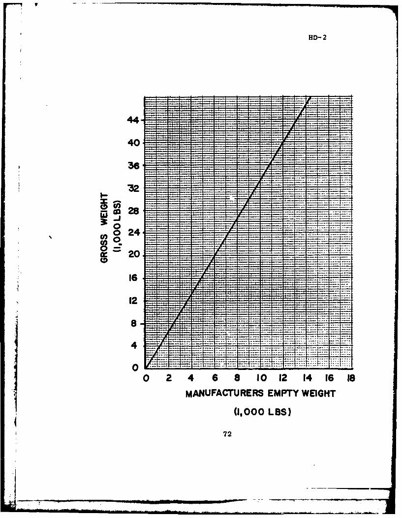
2.1 MAKE A ROUGH ESTIMATE OF THE MANUFACTURER'S EMPTY

WEIGHT.

Use the specification maximum gross weight from HD-1 and

the graph of historical weight ratios (HD-2) to estimate the

manufacturer's empty weight.

2.3 MAKE A ROUGH ESTIMATE OF GROSS WEIGHT.

Begin with an estimated gross weight which is 80% of the

specification value of gross weight.

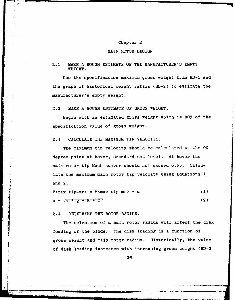
2.4 CALCULATE THE MAXIMUM TIP VELOCITY.

The maximum tip velocity should be calculated a-. he 90

degree point at hover, standard sea le-el. At hover the

main rotor tip Mach number should no, exceed 0.65. Calcu-

late the maximum main rotor tip velocity using Equations 1

and 2.

V<max tip-mr> = M<max tip-mr> * a (1)

a = .y * g ' H * T (2)

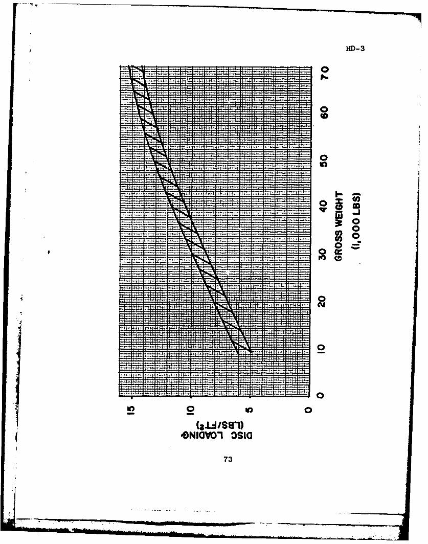
2.4 DETERMINE THE ROTOR RADIUS.

The selection of a main rotor radius will affect the disk

loading of the blade. The disk loading is a function of

gross weight and main rotor radius. Historically, the value

of disk loading increases with increasing gross weight (HD-3

26

4.A6:-

shows this trend). Use Equation 3 to calculate a rotor

radius which will optimize disk loading for the gross weight

estimate. Note that the maximum allowable radius is given

as a specification in HD-1.

R<mr> = VW<gross> / (DL * 7) (3)

2.5 DETERMINE A FIRST-CUT ROTATIONAL VELOCITY.

The maximum rotational velocity can be determined since

the maximum tip velocity and the design rotor radius are

known. Use Equation 4 to calculate the first-3ut rotational

velocity.

Q<mr-max> = V<max tip-mr> / R<mr> (4)

2.6 MAKE A FIRST-CUT DETERMINATION OF THRUST COEFFICIENT.

The first-cut value of thrust coefficient should be

determined at the specification density altitude using

Equation 5. The tip velocity is found using Equation 6 with

the main rotor radius found in Step 2.4 and the rotational

velocity found in Step 2.5. Thrust should be set equal to

the value of gross weight found in Step 2.2.

C<thrust-mr> = T<mr> / [A<mr> * 0 * V<tip-mr>2] (5)

V<tip-mr> = Q<mr> * R<mr> (6)

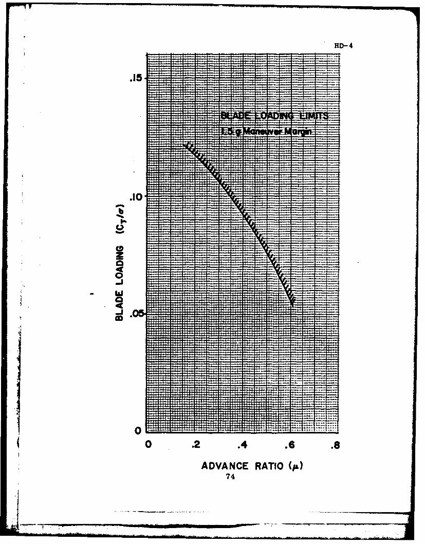
2.7 DETERMINE THE BLADE SOLIDITY.

Equation 7 can be used to find the maximum advance ratio.

The tip velocity was determined in Step 2.6 and the maximum

(forward velocity is given as a specification in HD-i. Once

27

the maximum advance ratio has been determined, HD-4 can be

used to determine the maximum blade loading. With this

maximum blade loading value and the main rotor thrust

coefficient from Step 2.6, calculate the solidity using

Equation 8.

il<max-mr> = V<max fwd> / V<tip-mr> (7)

a<mr> = C<thrust-mr> / BL (8)

2.8 DETERMINE THE NUMBER OF MAIN ROTOR BLADES TO BE USED.

The number of rotor blades to be used is a function of

rotor radius (as it affects solidity), vibration, and

weight.

For a given solidity, more blades would be required if

the radius and chord are to be ke~t small.

.The vibration of the main rotor is a factor in the

determination of the number of blades to be used. The

airframe can be expected to vibrate at the rotor harmonic

frequency and at integer multiples of the rotor frequency.

This integer multiple corresponds to the number of blades.

A vibration with a frequency of 1/REV (4 Hz) may occur which

could be caused by rotor unbalance, a blade out of track,

differences between blades, or a combination of these

factors. A vibration will also occur at the blade passage

frequency (b<mr> / REV). Vibrations of the rotor blades

induce loads which are summed at the hub and passed to the

airframe. A perfect rotor with all blades identical will

28

. . .. . .. . .. . . ..

act as a filter, so that only the (b<mr> / REV) and

multiples of (b<mr> / REV) are passed to the airframe [Ref.

2]. Therefore, the effect of main rotor vibration on the

airframe can be reduced by increasing the number of blades.

Note that the positive effects of reduced vibration and

smaller blades are offset by an increase in weight and hub

complexity. Select the number of blades for design and

include a brief analysis of your decision in the final

report.

2.9 DETERMINE THE CHORD AND THE ASPECT RATIO.

The chord can be calculated from Equation 9, since the

solidity (Step 2.7), the number of blades (Step 2.8), and

the rotor radius (Step 2.4) are known.

For a helicopter rotor, the aspect ratio is defined as

the radius divided by the chord. Historically, the main

rotor aspect ratio has been between 15 to 20, The aspect

ratio can be found using Equation 10 and the radius found in

Step 2.4. Adjust the value of rotational velocity (Step

2.5) as necessary, in order to obtain an aspect ratio of 15

to 20. If the rotational velocity is reduced, then Steps

2.6 and 2.7 must be recalculated.

c<mr> = (a<mr> * 1 * R<mr>) / b<mr> (9)

AR<mr> = R<mr> / c<mr> (10)

29

ij ... .

2.10 DETERMINE THE AVERAGE LIFT COEFFICIENT.

The average lift coefficient is a function of thrust

coefficient and solidity as shown in Equation 11.

C<lift> = ( 6 * C<thrust-mr> ) / a<mr> (11)

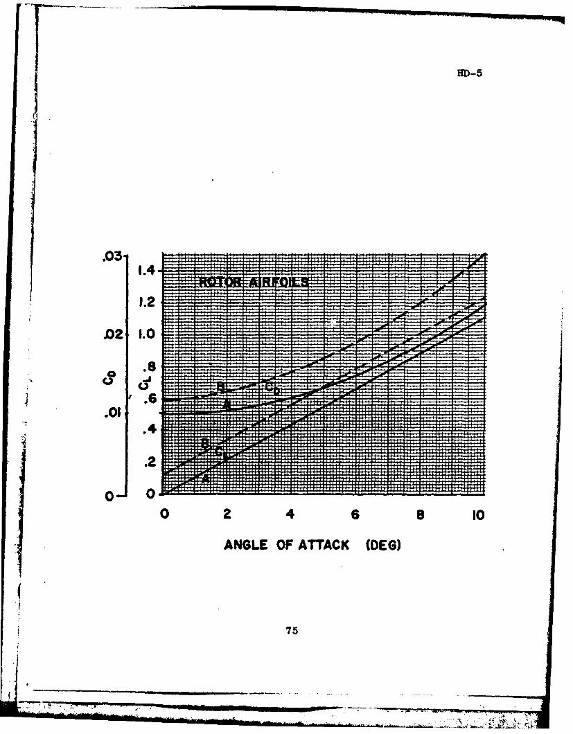
2.11 CHOOSE AN AIRFOIL SECTION FOR THE MAIN ROTOR BLADES.

The selection criteria for an airfoil are [Ref. 3]:

A) high stall angle of attack to avoid stall on the

retreating side,

B) high lift curve slope to avoid operation at high

angles of attack,

C) high maximum lift coefficient to provide the neces-

sary lift,

D) high drag divergence Mach number to avoid com-

pressibility effects on the advancing side,

E) low drag at combinations of angles of attack and Mach

numbers represeating conditions at hover and cruise,

and

F) low pitching moments to avoid high control loads and

excessive twisting of the blades.

Historically, the NACA 0012 airfoil has been used most often.

The primary sources for making your selection should be HD-5

and Theory of Wing Sections [Ref. 4]. Choose one of the

airfoils from HD-5 or select one from Reference 4. Your

final report should include a brief discussion of the rea-

sons for your selection.

30L7:7

2.12 DETERlMINE AVERAGE LIFT CURVE SLOPE AND AVERAGE

PROFILE DRAG COEFFICIENT.

If you selected one of the blades from HD-5, then use

HD-5 to determine the profile drag coefficient and the lift

curve slope (C If another airfoil was chosen, then

- use Reference 4 to determine the profile drag coefficient

and the lift curve slope. DATCOM [Ref. 5] can also be ased

to find the lift curve slope.

II

(31

I ii. . .. ..

Chapter 3

PRELIMINARY POWER CALCULATIONS

3.1 MAKE FIRST ESTIMATE OF THE POWER REQUIRED TO HOVER.

The total power required to hover out-of-ground effect

at standard sea level is the induced power (out-of-ground

effect with tiploss) added to the profile power. Compute

the power required to hover out-of-ground effect at standard

sea level using Equations 12 through 15. An HP-41CV program

entitled HOVER [Ref. 6) can be also used to compute these

values

B<mr> = 1 - [ v' 2 * C<thrust-mr* / b<mr> ] (12)

Pi<mr-TL> = (1/B<mr,) * [T<mr>- s / 2 * * A<mr> ] (33)

Po<mr> - O.125*c<mr>*Cdo<mr>*o*A<mr>*V<Tip-mr>3 (14)

PT<mr-hover> = Pi<mr-TL> + Po<mr> (15)

3.2 MAKE SECOND GROSS WEIGHT ESTIMATE.

Gross weight, empty weight, rotor disc area, solidity,

and total power to hover (OGE, SSL) are variables in the

weight estimation formulas. Preliminary values have been

found for these variables in Steps 2.1, 2.2, 2.4, 2.7, and

3.1. Using HD-6, refine the first gross weight estimate

used in the main rotor design process. To estimate the fuel

weight required in HD-6, use the fuel capacity of a com-

parably sized helicopter in HD-7. The useful load is

32

• ~~~~~~- - -- - - - --- .---- ., ... . -2_

defined as the internal load capacity plus the crew weight

allowance. Use the format in Figure 1 for your report.

WEIGHT ESTIMATION TABLE

---------ITERATION----------FIRST SECOND THIRD

SOLIDITY:RADIUS:HOVER POWER:

ROTOR - BLADES:HUB/HINGES:TOTAL:

PROPULSION:FUSELAGE:

FLIGHT CONTROLS:ELECTRICAL:FIXED EQUIPMENT:

EMPTY:

FUEL:USEFUL LOAD:

GROSS:

Figure 1: Weight Estimation Format

3.3 ESTABLISH FIGURE OF MERIT AT APPROXIMATELY 0.75.

Historically, a Figure of Merit of 0.75 is considered

average [Ref. 2]. If the induced power is between 70 to 80%

of the total power, the Figure of Merit will be approxi-

mately 0.75. Recalculate the hover power (Step 3.1)

using the new gross weight estimate calculated in Step 3.2.

For small gross weight changes the value of disk loading may

be adjusted provided it remains within the limits defined by

33

WC

HD-3. If a significant gross weight change occurs, a radius

change should be made in Step 2.3 to keep disk loading

within limits. If the main rotor radius is changed, then

Steps 2.5, 2.6, 2.7, and 2.10 must be recalculated. Verify

that the new value of induced power is between 70 to 80% of

the new total power. If not, the geometric parameters must

be changed to obtain that relationship. Hint: If the

induced power is greater than 80% of the total power, then

increase the chord length. An increase in the value of

chord length increases solidity and decreases blade loading.

The maximum value of blade loading was used in Step 2.7 and

lower blade loadings are desirable. If the chord length is

increased, Steps 2.7, 2.9, and 2.10 must be recalculated.

If the chord length cannot be increased without violating

the limits of aspect ratio, then the radius or the

rotational velocity should be changed. If the induced power

is less than 70% of the total power, then reduce the

rotational velocity. In Step 2.5, a maximum tip velocity

was used which could be lowered slightly. A reduction in

the rotational velocity increases the advance ratio which

decreases the blade loading (see HD-4).

3.4 REFINE SECOND GROSS WEIGHT ESTIMATE.

Since the hover power (and possibly solidity or area) was

adjusted, refine the gross weight using HD-6. List the new

34

weight estimates (third iteration) in your report as per the

format of Figure 1.

3.5 MAKE THIRD ESTIMATE OF POWER REQUIRED TO HOVER.

Refine the power required to hover out-of-ground effect

(Step 3.2) using the revised gross weight (Step 3.4).

:3.6 REPEAT THE GROSS WEIGHT ESTIMATE AND THE HOVER POWER

REQUIRED ITERATION.

Repeat the iterations (Steps 3.3, 3.4, and 3.5) until

successive steps converge at less than 10% difference.

:3.7 DETERMINE THE POWER REQUIRED TO HOVER IGE, SSL.

The profile power stays the same as for hover OGE (Step

:3.1), but the induced power gets smaller. Calculate the

hover power in ground effect using Equations 15 through 17.

An HP-41CV program entitled HOVER [Ref. 67 can also be used

to compute these values. Use a hover height of 10 feet

above ground level for your calculations.

Pi<mr-TL+GE> - (P/P<OGE>) * Pi<mr-TL> (15)

P/P<OGE> = - 0.1276(h/D) = 0.7080(h/D)3 - 1.4569(h/D) 2 (16)

+ 1.3432(h/D) + 0.5147

PT<mr-hover> = Pi<mr-TL+GE> + Po<mr> (17)

3.8 DETERMINE THE PARASITE POWER REQUIRED IN FORWARD

FLIGHT

Equation 18 shows the relationship between the equivalent

flat plate area loading and the parasite power required in

( forward flight. There are several methods that can be used

35

to determine the equivalent flat plate area in forward

flight. One method is to use HD-8 and the latest estimate

of gross weight to find the equivalent flat plate area

loading, then to use Equation 19 to find the equivalent flat

plate area in forward flight.

Pp<fwd> = 0.5 * p * V<fwd>3 * EFPA<FF> (18)

EFPA<FF> U W<gross> / Loading<EFPA> (19)

3.9 DETERMINE MAIN ROTOR POWER REQUIRED AND THE MACH

NUMBER OF THE ADVANCING BLADE TIP FOR FORWARD FLIGHT.

These calculations should be made at both standard sea

level and at specification density altitude using Equations

20 through 26. Create tables with the velocity incremented

at least every 20 knots. The cruise velocity should also be

included. Two programs have been developed either of which

could also be used to calculate these values: a FORTRAN

program entitled Helicopter Power Computation Package [Ref.

7] for use on the IBM-3033, and a program entitled FLITE

[Ref. 8] for use with the HP-41CV programmable calculator.

Use the format shown in Figure 2 for your report.

mu<mr> = V<fwd> / V<tip-mr> (20)

Po<mr-fwd> = [1 + 4.3*u<mr> 2 ] * Po<mr-hover> (21)

Vi = V T<mr> / [2 * p * 7 * R<mr>l]' (22)

Vi<T>4 + 2*V<vert>*Vi<T> 3 + (23)

[V<fwd> 2 + V<vert>z]*Vi<T> 2 - Vi4 = 0

Pi<mr-TL-fwd> = (1/B<mr>) * T<mr> * Vi<T> (24)

36

' ' , , m n i i i l. ......'...........i ..... . . .... ...

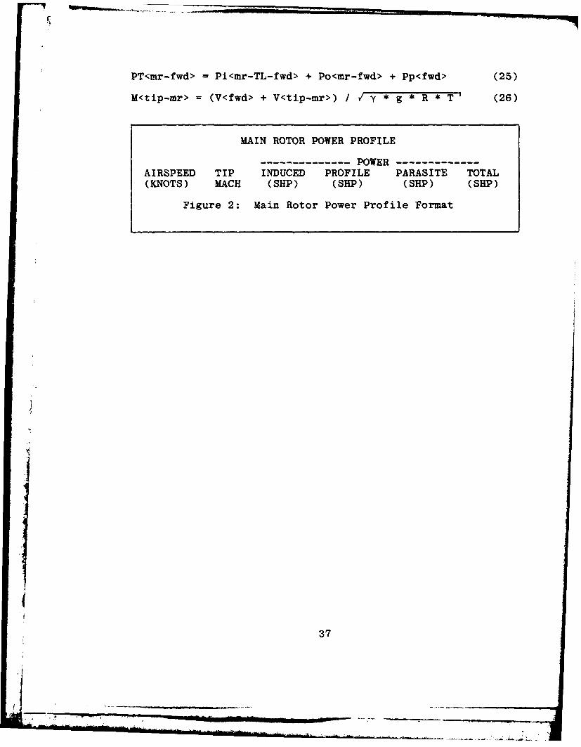
PT<mr-fwd> =Pi<nir-TL-fwd> + Po<mr-fwd> + Pp<fwd> (25)

M<tip-mr> =(V<fwd> + V<tip-mr>) /.y *g * R * T' (26)

MAIN ROTOR POWER PROFILE

---------------------------------- POWER---------------AIRSPEED TIP INDUCED PROFILE PARASITE TOTAL(KNOTS) MACH (SHiP) (SHiP) (SHiP) (SHiP)

Figure 2: Main Rotor Power Profile Format

37

Chapter 4

TAIL ROTOR DESIGN

4.1 MAKE PRELIMINARY DETERMINATIONS OF TAIL ROTOR

GEOMETRY.

Use HD-9 in your determination of radius, rotational

velocity, drag coefficient, and the number of blades. The

length of the fuselage from the center-of-gravity to the

tail rotor hub should be calculated using Equation 27. The

chord can be determined by Equation 28 and the use of a.

value of tail rotor aspect ratio within the historical range

of 4.5 to 8.0. Use Equation 29 to calculate the tail zotor

solidity.

L<tr> = R<mr> + R<tr> + 0.5 ft (27)

c<tr> = R<tr> / AR<tr> (28)

c<tr> = b<tr> * c<tr> / (7 * R<tr>) (29)

4.2 DETERMINE TAIL ROTOR POWER REQUIRED AT HOVER OGE, SSL.

The total power of the tail rotor required to hover

out-of-ground effect at standard sea level is the induced

power, out-of-ground effect with tiploss, added to the

profile power. Use Equations 30 through 36 to determine the

tail rotor hover power. The HP-41CV programs entitled TR or

Hover [Ref. 6] can be used to compute these values.

T<tr> = PT<mr-hover> / ( Q<mr> * L<tr> ) (30)

C<thrust-tr> = T<tr> / [A<tr> * * V<tip-tr>2 ] (31)

38

.. .... . .

V':tip-tr> = <tr>* R<tr> (32)

B<tr> = 1 -[ V2 * Ccthrust-tr> '/b<tr> 1(33)

Pi<tr-TL> =(i/B<tr>) * [T<tr> 1* / 2 * g* A~tr> '] (34)

Po<tr> = 0.125*a<tr>*Cdo<tr>*P*A~tr>*V<tip-tr>3 (35)

PT<tr-hover'> = Pi<tr-TL> + Po~tr> (36)

4.3 DETERMINE TAIL ROTOR POWER REQUIRED AND TIP MACH

EFFECTS FOR FORWARDl FLIGHT.

These calculations should be made at both standard sea

level and at specification density altitude using Equations

37 through 46. Create tables with the velocity incremented

at least every 20 knots. The cruise velocity should also be

included. The computer program [Ref. 7] and the HP-41CV

program [Ref. 8] mentioned in Step 3.9 can also be used to

calculate these values. Use the format shown in Figure 3

for your report.

ut>= V<fwd> / V<tip-tr> (37)

Po<tr-fwd> = Po<tr-hover> * [1 + 4.3 * j<tr> 2] (38)

T<tr> = PT<mr-fwd> / (2<mr> * L<tr> )(39)

C<thrust-tr> =T<tr> / [A<tr> * o * V<tip-tr>2 (40)

B<tr> = 1 -[ 2 * C<thrust-tr>'/ b<tr> ](41)

Vi = T<tr> /[2 * o * 7r * R<tr>/]' (42)

Vi<T>4 + 2*V<vert>*Vi<T> 3 + (43)I[V<fwd >2 + V~vert >2])*Vi<T> 2 _ Vi4 = 0

Pi<tr-TL-fwd> - (lfBmr>) * T<tr> * Vi<T> (44)PT<tr-fwd> =Pi<tr-TL-fwd> + Po<tr-fwd> (45)

Mctip-tr> (V<fwd> + V<tip-tr>) y ~ g *R *T (46)

39

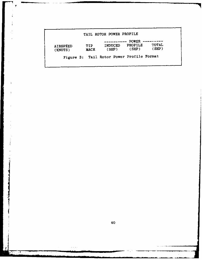
TAIL ROTOR POWER PROFILE

---------------------------------- POWER ----------

AIRSPEED TIP INDUCED PROFILE TOTAL

(KNOTS) MACH (SHP) (SHP) (SHIP)

Figure 3: Tail Rotor Power Profile Format

40

Chapter 5

POWER CALCULATION REFINEMENTS

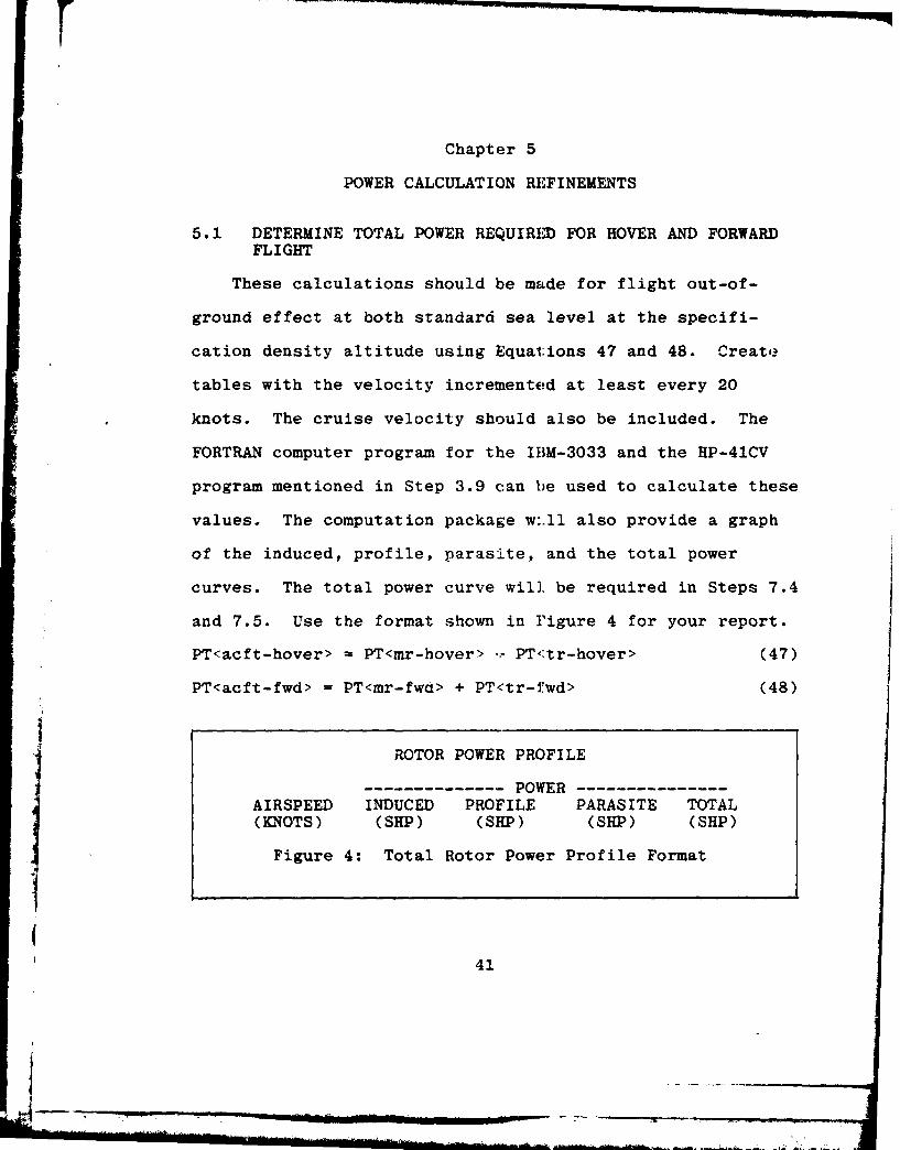
5.1 DETERMINE TOTAL POWER REQUIRI) FOR HOVER AND FORWARD

FLIGHT

These calculations should be made for flight out-of-

ground effect at both standard sea level at the specifi-

cation density altitude using Equations 47 and 48. Create

tables with the velocity incremented at least every 20

knots. The cruise velocity should also be included. The

FORTRAN computer program for the IBM-3033 and the HP-41CV

program mentioned in Step 3.9 can be used to calculate these

values. The computation package w:.ll also provide a graph

of the induced, profile, parasite, and the total power

curves. The total power curve will be required in Steps 7.4

and 7.5. Use the format shown in Figure 4 for your report.

PT<acft-hover> = PT<mr-hover> .i PT<:tr-hover> (47)

PT<acft-fwd> = PT<mr-fwu> + PT<tr-fwd> (48)

ROTOR POWER PROFILE

---------------POWER---------------AIRSPEED INDUCED PROFILE PARASITE TOTAL(KNOTS) (SHP) (SHP) (SHP) (SHP)

Figure 4: Total Rotor Power Profile Format

41

5.2 DETERMINE COMPRESSIBILITY CORRECTION.

When an airfoil is operated at a Mach number of 1.0 or

greater, pressure disturbances caused by the airfoil cannot

propagate forward and shock waves will form ahead of the

airfoil. The noise level produced by the rotor is greatly

increased when the shock waves form [Ref. 9]. Weak oblique

shock waves can form at local points on the airfoil even

before the free stream reaches Mach 1.0. The free stream

Mach number at which any local Mach number reaches 1.0 is

called the critical Mach number. Above this critical Mach

number, drag begins to increase. Therefore, additional

power is required to overcome the effects of compressibility

on the performance of a helicopter rotor. Use Equations 49

through 51 to calculate the compressibility correction, at

both standard sea level and the specification density

altitude. Note that Equation 50 has been adjusted by 0.06

in order to agree with experimental data for a NACA 0012

airfoil [Ref. 10]. Assume this equation applies for any

airfoil. The compressibility correction should be

determined only at the highest Mach number (usually at the

maximum velocity). The values of critical Mach number can

be found in HD-IO. Use the lowest value of critical Mach

number (at the highest angle of attack) for your calculations.

P<Comp> P * A<mr> * V<tip-mr> 3 * o<mr> (49)

* [0.012*Md + 0.10*Md3 ]

42

Md M<tip-mr> - M<Crit> - 0.06 (50)

M<tip-mr> = (V<tip-mr> + V<fwd>) / y * g * R * T1 (51)

5.3 DETERMINE THE REQUIRED RSHP AT MAXIMUM VELOCITY.

Add the appropriate compressibility corrections from Step

5.2 to the values of total power at maximum velocity

determined in Step 5.1 (for both standard sea level and the

specification density altitude). After adding the compressi-

bility corrections, the higher of the two values should be

used as the required rotor shaft horsepower.

5.4 DETERMINE THE REQUIRED RSHP FOR HOVER (IGE) AT THE

SPECIFIED CEILING.

Use the gross weight tha ; has been used since Step 3.6

and note that the density wi'l be different at the

specification hover ceiling. The specification hover

ceiling can be found in HD-1. Use Equations 52 through 59

to calculate the main rotor hover power and the equations

provided in Step 4.2 to calculate the tail rotor hover power

at the specification hover ceiling. Assume a hover height

of 10 feet above ground level. The HP-41CV programs

entitled HOVER and TR (Ref. 6] can be used to compute these

values. The required RSHP for hover is the aircraft total

hover power.

C<thrust-mr> = T<mr> / [A<mr> * * V<tip-mr> 2 ] (52)

B<mr> = 1 - [ 2 * C<thrust-mr> / b<mr> ] (53)

Pi<mr-TL> = (I/B<mr>) * [T<mr>- / 2 * p * A<mr> ] (54)

43

Pi<mr-TL+GE> = (P/P<OGE>) * Pi<mr-TL> (55)

P/P<OGE = - 0.1276(h/D)" + 0.7080(h/D)3 - 1.4569(h/D)2 (56)

+ 1.3432(h/D) + 0.5147

Po<mr> - O.125*c<mr>*Cdo<mr>*p*A<mr>*V<tip-mr>s (57)

PT<mr-hover> = Pi<mr-TL-GE> + Po<mr> (58)

PT<acft-hover> = PT<mr-hover> + PT<tr-hover> (59)

5.5 DETERMINE THE TOTAL ESHP REQUIRED.

Compare the values of RSHP found in Steps 5.3 and 5.4.

The greater of these two values is the maximum required

RSHP, which should be used to find the required ESHP. The

engine shaft horsepower is defined as the rotor shaft

horsepower adjusted for transmission and accessory losses.

Use Equation 60 to calculate ESHP, assuming:

A) ten horsepower for accessories,

B) ten percent losses in SHP for multiple engine

4installation, and

C) three percent transmission losses.

ESHP<Req> [0.10 * RSHP<max> * (n-i)] (60)

+ 1.03 * RSHP<max> + 10.0 hp

44i 44

.... ....... " ' '- :" : -11 f i Ii °if l i I ................................. ,.......................'....."............;. '

Chapter 6

ENGINE SELECTION

6.1 SELECT TYPE AND NUMBER OF ENGINES.

The number of engines to be used should be determined by

considering the factors of safety, survivability, and

reliability. Select the number of engines based on these

considerations and briefly explain your decision in your

final report. Remember that in Step 5.4 multiple engine

installation was considered. If you decide to use a

different number of engines, go back to Step 5.4 and

recompute ESHP.

The criteria for selection of the type of engine to be

used are weight, life-cycle costs, availability,

reliability, maintainability, and performance.

The weight of the engine should be as small as possible.

The life-cycle costs can be computed using the data found

in HD-i and HD-li. The life-cycle costs are the summation

of the research and development costs, the initial cost, the

yearly operating cost (average value, adjusted for

inflation), the yearly maintenance cost (average value

including overhauls, adjusted for inflation), the

replacement cost (if the life of the engine is less than the

life of the helicopter) and the salvage value. In order to

compute the life-cycle costs, the expected time of service

45

of the helicopter in years, the expected number of flight

hours per year of the helicopter, and the expected engine

life (sometimes called mean time between replacements) in

hours must be known. If the engine life in hours is less

than the helicopter life in hours, then the number of engine

replacements must be computed. To find the number of engine

replacements divide the helicopter life in hours by the

engine life in hours, round up to the next integer if there

is a remainder, then subtract 1.0 (the initial engine).

Equation 61 should be used to compute the life-cycle costs.

The availability is a function of the mean time between

maintenance actions and the maintenance down time. The

engine availability can be computed using the relationship

given by Equation 62 and tue appropriate values in HD-11.

The reliability of the engine is a function of the mean

time between failures (failure rate) and the length of the

average flight in hours (see HD-i). Equations 63 and 64 can

be used to compute the reliability.

The maintainability is a function of the mean time to

repair but is sometimes given as a fraction of the

maintenance down time in hours divided by the total flight

hours. Either measure can be used for comparison.

The performance of the engine can be measured in many

ways, but for this course the measure of performance will be

the shaft horsepower produced by the engine. Insure the

engine you select has a military ESHP greater than the

46

ESHP<Req> you found in Step 5.4. A computer program

entitled Helicopter Engine Program [Ref. 11] has been

developed that computes the shaft horsepower available at

any given altitude and airspeed for various engines;

however, this computation is done for a "rubber" engine and

should not be used if real engine data is available.

Once values have been determined for each criteria for

each competing engine, the designer must choose the engine

that best optimizes the six criteria mentioned above. In

order to select the "best" engine, the six criteria must be

weighted according to their importance. For example, high

performance and low weight may be more desirable than low

life-cycle cost. In order to establish uniform selection

criteria, the weighting factors for the six criteria are

given in HD-i1. Your final report should contain a

completed chart using the format of Figure 5 and a brief

discussion of the decision-making process you used in your

selection of an engine type. Compute the availability,

reliability, and maintainability on a per engine basis.

LCC = n*[RDC + IC + HL<yrs>*(YOC+YMC) + n<rpl>*(RC-SV)] (61)

AVAIL = MTBMA / ( MTBMA + MDT ) (62)

RELY = e(- <FR> * LAF<hrs>) (63)

X<FR> = 1 / MTBF (64)

47

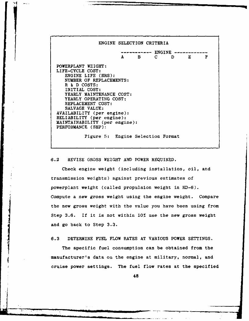
ENGINE SELECTION CRITERIA

----------- ENGINE------------A B C D E F

POWERPLANT WEIGHT:LIFE-CYCLE COST:

ENGINE LIFE (HRS):NUMBER OF REPLACEMENTS:R & D COSTS:INITIAL COST:YEARLY MAINTENANCE COST:YEARLY OPERATING COST:REPLACEMENT COST:SALVAGE VALUE:

AVAILABILITY (per engine):RELIABILITY (per engine):MAINTAINABILITY (per engine):PERFORMANCE (SHP):

Figure 5: Engine Selection Format

6.2 REVISE GROSS WEIGHT AND POWER REQUIRED.

Check engine weight (including installation, oil, and

transmission weights) against previous estimates of

powerplant weight (called propulsion weight in HD-6).

Compute a new gross weight using the engine weight. Compare

the new gross weight with the value you have been using from

Step 3.6. If it is not within 10% use the new gross weight

and go back to Step 3.3.

6.3 DETERMINE FUEL FLOW RATES AT VARIOUS POWER SETTINGS.

The specific fuel consumption can be obtained from the

manufacturer's data on the engine at military, normal, and

cruise power settings. The fuel flow rates at the specified

48

power settings can then be determined ofl a per engine basis

from Equation 65.

Wf SFC *SHP (65)

49

Chapter 7

RANGE AND ENDURANCE CALCULATIONS

7.1 DETERMINE THE SLOPE OF THE FUEL FLOW VERSUS SHP LINE

AND THE ZERO HORSEPOWER INTERCEPT.

These calculations should be made at standard sea level.

The relationship between fuel flow rate and shaft horsepower

for a turboshaft engine is fairly linear except at low

values of shaft horsepower. The average slope of the fuel

flow versus SHP line can be found mathematically using the

values of fuEl flow rate at the military, normal, and cruise

power settings calculated in Step 6.3. The intercept of the

fuel flow versus SHP line with the ordinate axis is the zero

horsepower intercept.

FUEL 1FLOW J

RATE

ZHI

SHAFT HORSEPOWER

Figure 6: Zero Horsepower Intercept

50

- -- ,.---.- ~. .... . .----

B<ave> = A Wf / A SHP (66)

7.2 COMPUTE THE ZERO HORSEPOWER INTERCEPT AT SPECIFICATION

CONDITIONS.

At standard sea level, both 0 and 5 are equal to 1.0;

therefore, the value of a can be determined using the zero

horsepower intercept found in Step 7.1. Find e and S at the

specification pressure altitude using Equations 67 and 68,

then calculate the zero horsepower intercept using Equation

69. The pressure at the specification pressure altitude

can be found using an ICAO standard atmospheric table. The

temperature at the specification pressure altitude is given

in RD-i.

e<spec> = T<spec> / T<SSL> (67)

S<spec> = P<spec> / P<SSL> (68)

ZHI = a<ave> * 6 * (69)

7.3 DETERMINE THE ZERO HORSEPOWER INCREMENT.

The value of the zero horsepower increment is based on

the number of engines, the zero horsepower intercept, and

the fuel flow rate per horsepower. The slope of the fuel

flow versus SHP line is the same at all density altitudes.

These calculations should be made at the specification

density altitude. The zero horsepower increment is

sometimes called the phantom SHP. Use Equation 70 to

calculate the phantom SHP.

P<SHP> = [n * a<ave> * 8 * T' ] / 3<ave> (70)

51

* _______________________________________

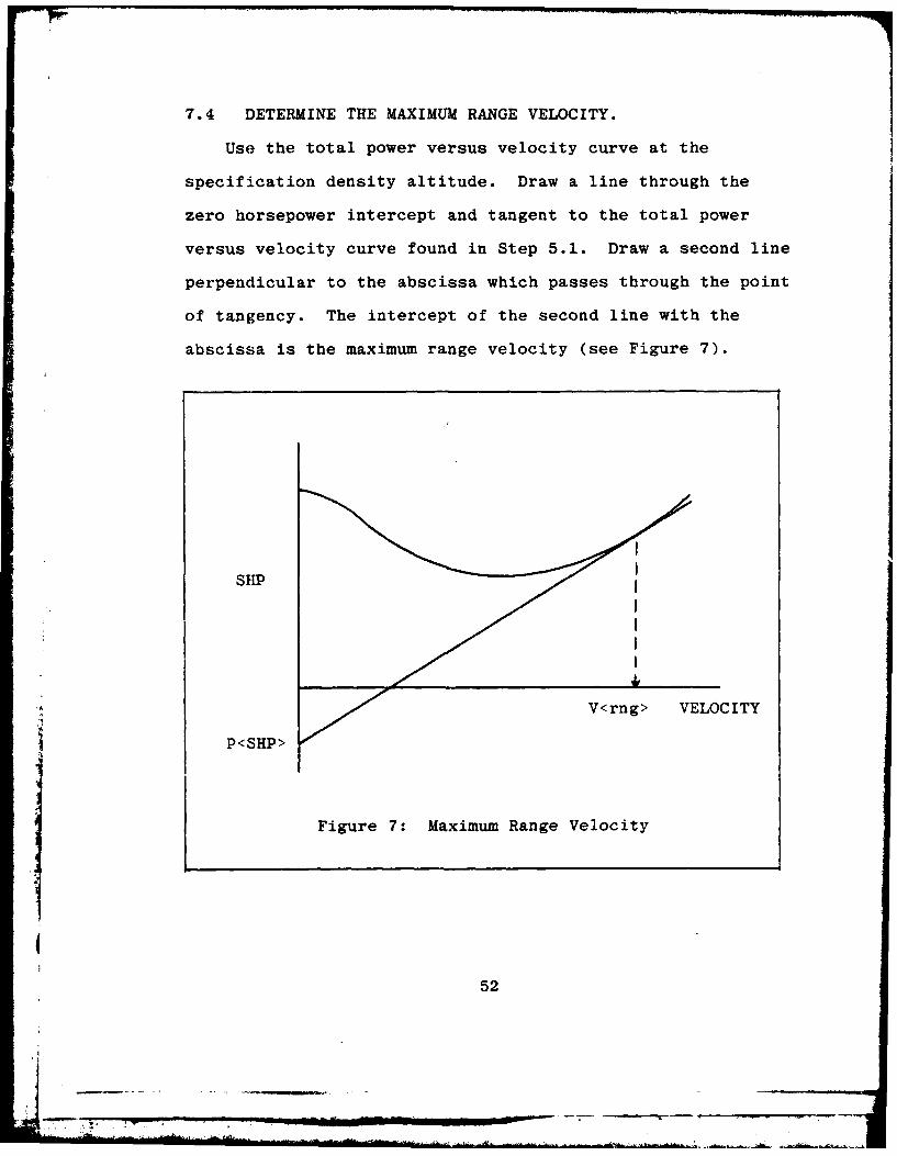
7.4 DETERMINE THE MAXIMUM RANGE VELOCITY.

Use the total power versus velocity curve at the

specification density altitude. Draw a line through the

zero horsepower intercept and tangent to the total power

versus velocity curve found in Step 5.1. Draw a second line

perpendicular to the abscissa which passes through the point

of tangency. The intercept of the second line with the

abscissa is the maximum range velocity (see Figure 7).

Slip

V<rng> VELOCITY

P<SHP>

Figure 7: Maximum Range Velocity

52

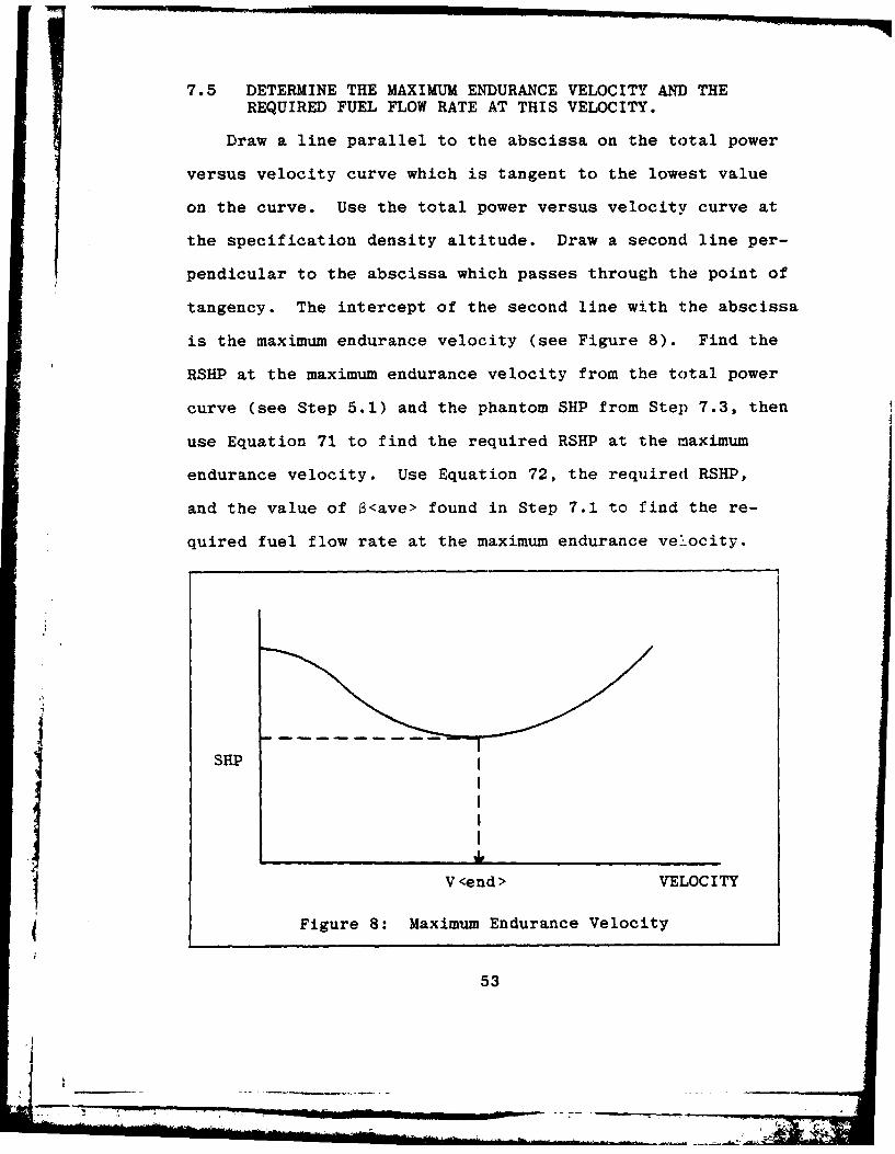
7.5 DETERMINE THE MAXIMUM ENDURANCE VELOCITY AND THE

REQUIRED FUEL FLOW RATE AT THIS VELOCITY.

Draw a line parallel to the abscissa on the total power

versus velocity curve which is tangent to the lowest value

on the curve. Use the total power versus velocity curve at

the specification density altitude. Draw a second line per-

pendicular to the abscissa which passes through the point of

tangency. The intercept of the second line with the abscissa

is the maximum endurance velocity (see Figure 8). Find the

RSHP at the maximum endurance velocity from the total power

curve (see Step 5.1) and the phantom SHP from Step 7.3, then

use Equation 71 to find the required RSHP at the maximum

endurance velocity. Use Equation 72, the required RSHP,

and the value of <ave> found in Step 7.1 to find the re-

quired fuel flow rate at the maximum endurance velocity.

SHP

tjV<end> VELOCITY

Figure 8: Maximum Endurance Velocity

53

RSHP<Req-max end> = P<SHP> + RSHP<max end> (71)

Wf<max end> = RSHP<Req-max end> * S<ave> (72)

7.6 DETERMINE THE POWER REQUIRED AT SPECIFICATION CRUISEVELOCITY AND THE REQUIRED FUEL FLOW RATE AT THISVELOCITY.

Find the RSHP at cruise velocity from the total power

curve at the specification density altitude (see Step 5.1)

and add the phantom SHP found in Step 7.3. This sum (see

Equation 73) is the required RSHP at cruise velocity. After

computing the required RSHP, use Equation 74 to find the

fuel flow rate at cruise velocity.

RSHP<Req-cruise> = P<SHP> + RSHP<cruise> (73)

Wf<cruise> = RSHP<Req-cruise> * <ave> (74)

7.7 DETERMINE THE TOTAL FUEL REQUIREMENTS FOR SPECIFIED

MAXIMUM RANGE.

The total fuel requirements are based on the following

assumptions:

A) warm-up and take-off requires three minutes of fuel at

normal rated power,

B) cruise at specification velocity,

C) approach and landing requires three minutes of fuel at

normal rated power, and

D) reserve requires fifteen minutes at maximum endurance

velocity.

The cruise velocity and the maximum range are specifications

and can be obtained from HD-1. Use Equation 75 to find the

fuel weight. Assume the fuel flow rates are constant.

54

t2 i '' . - ....-- - -- , - J i , -% w .- - :

FYI 0 .05*n*Wf<NRP> + [(Wf~cruise>*RNG<max>)/V<Cruise>1 (75)

+ O.05*n*Wf<NRP> + O.25*Wf<max end>

55

....................... i

Chapter 8

MISCELLANEOUS CALCULATIONS

8.1 COMPUTE DESIGN GROSS AND EMPTY WEIGHT.

At this point, your power calculations have been made

with an estimated gross weight from Step 3.6 which is

different from the design gross weight. The design gross

weight includes the actual powerplant weight from Step 6.1

and the actual fuel weight from Step 7.7. If the design

gross weight is greater than the estimated gross weight,

return to Step 3.3. If the design gross weight is less

than the estimated gross weight, increase the fuel weight or

the internal load capacity so that the design gross weight

equals the estimated gross weight. Note that specifications

may be exceeded if the change is advantageous. If the fuel

weight is increased in this manner, the maximum range must

be recomputed (See Step 7.7).

8.2 DETERMINE RETREATING BLADE STALL VELOCITY.

The retreating blade stall velocity can be calculated

using a technique developed in Reference 10. A program for

the HP-41CV programmable calculator entitled BS [Ref. 12]

has been developed utilizing this technique which can be

used to calculate the retreating blade stall velocity. The

program uses the geometric design parameters of the main

56

!

rotor and the aircraft's forward velocity as input, then

outputs the maximum angle of attack at the 270 degree point,

the amount of collective set, and the amount of cyclic that

is set. The cyclic will be negative for forward flight.

The program assumes that the maximum unstalled angle of

attack is 12.5 degrees, that the effective dimensionless

radius is 0.97 and that there is no lateral flapping. Note

that the slope of the lift curve was found in Step 2.12 and

that a value of the twist of the main rotor blade is

required. (Assume a linear twist of -10 degrees.)

To determine the retreating blade stall velocity at

standard sea level, run the program using various forward

velocities until the program indicates that the retreating

blade has stalled (use the greatest unstalled velocity) or

until the specification maximum velocity is reached.

Equations 76 through 92 may also be used to determine the

retreating blade stall velocity at standard sea level in

lieu of the HP-41CV program. (The assumptions mentioned

above also apply to these equations.) First, determine if

the blade is stalled by comparing the angle of attack of the

main rotor at the 270 degree position with the maximum angle

of attack. Second, reduce the forward velocity if the

maximum angle of attack (12.5 degrees) is exceeded and

iterate to find the greatest unstalled forward velocity.

Note that Equations 90 and 91 must be solved simultaneously

for the collective and cyclic angles in radians and that

57

Equation 92 yields the angle of attack at the 270 degree

position in degrees.

T<I> = 0.4705 + 0.5000 * u<mr>2 (76)

T<2> = 0.3042 + 0.4850 * u<mr> 2 (77)

T<3> = 0.2213 + 0.2352 * ui<mr> 2 (78)

T<4> = 0.2352 * P<mr> + 0.1250 * v<mr> 2 (79)

A<D> = 0.9409 - 0.5000 * u<mr> 2 (80)

A<I> = [2.0000 * u<mr> - 0.5314 * u<mr>3 ] I A<D> (81)

A<2> = [2.5867 * u<mr>] / A<D> (82)

A<3> = [1.9400 * i<mr>] / A<D> (83)

A<4> - [0.9409 = 1.5000 * v<mr>:] / A<D> (84)

a = [0.0012 * EFPA<FF> * V<fwd>3 ] / W<gross> (85)

w = W<gross> / [0.0149 * R<mr> 2 * V~fwd>] (86)

= (V<fwd> * a - w) /(Q<mr> * R<mr>) (87)

C<thrust> = W<gross> / [0.0075 * R<rnr>'> * 2<mr>2 ] (88)

Z = (2 * C<thrust>) /(CL,Os * i<mr>) (89)

0.0 = a * A<1> + e<o> * A<2> (90)

+ 8<t> * A<3> + 6<v> * A<4>

Z = a * T<I> + 9<o> * T<2> (91)

+ 9<t> * T<3> + 9<y> * T<4>

a<270> = [(A/ 1+u<mr>) - <y> (92)

+ 6<o> + O<t>] * 57.3

8.3 DETERMINE BEST RATE OF CLIMB.

The best rate of climb occurs in forward flight in the

vicinity of the minimum total power on the total main rotor

58

I---

power curve. The following procedure should be used in

order to find the best rate of climb:

A) select a velocity near the lowest point on the rotor

total power curve (SSL),

B) compute the rotor total power available using Equa-

tion 93 (ESHP<Avail> is the military rated power at

SSL multiplied by the number of engines),

C) guess a value of vertical velocity,

D) solve for the thrust component of induced velocity

using Equations 94 and 95,

E) calculate the induced, profile, parasite, and climb

power using Equations 96 through 100,

F) compute main rotor total power using Equation 101,

then add the tail rotor total power calculated using

the equations in Step 4.3 and compare with the total

rotor power available, and

G) repeat the process until the total rotor power is

equal to the total rotor power available or until the

main rotor induced power equals zero.

The HP-41CV programs called FLIGHT and TR [Ref. 5] can be

used to compute the main rotor power and the tail rotor

power. The final value of vertical velocity is the best

rate of climb.

PT<Avail> = (ESHP<Avail>-10.0) / (0.10*(n-1)+1.03) (93)

Vi - T<mr> / [2 * P * *"R<mr>2] ' (94)

59

Vi<T>4 + 2*V<vert>*Vi<T>3 + (95)

[V<fwd>2 + V<vert> 21*Vi<T>2 -V14 = 0

Pp<mr> = (O.5*p*EFPA<VF>*V<vert> 3 1 (96)

+ (O.5*P*EFPA<FF>*V<fwd>3 ]

Po<mr> - O.125*P*Cdo<mr>*r<zr>*A.~mr>*V<tip-mr >3 (97)

*[1 + 4.3*uj<mr> 2 1

EFPA<VF> = 2 * EFPA<FF> (98)

Pc = Tcmr> *V<vert> (99)

Pi<umr-TL> =(1/B<mr>) * T<mr> *Vi<T> (100)

PT<mr-fwd climb> = Po<mr> +- Pi<mr-TL> + Pc + Pp<mr> (101)

8.4 COMPUTE MAXIMUM HOVER ALTITUDE (IGE).

Calculate the highest altitude at which the helicopter

can hover in ground effect using tte following method:

A) assume a hover height of 10 feet above ground level,

B) guess an al'titude,

41 C) compute the total power requiired to hover in ground

effect using the equations given in Step 5.1,

D) compare the total power required with the total power

available found in Step 8.3 (assume power available

remains constant with increasing altitude) and

repeat the process if they are not equal.

The altitude at which the total power required equals the

total power available is the maximum hover altitude in

ground effect.

60

8.5 COMPUTE SERVICE CEILING.

Service ceiling is defined as the maximum altitude at

which the helicopter exhibits a 100 fpm rate of climb

capability at a given temperature. It is normally defined

at the best rate of climb velocity using the normal engine

power rating. The service ceiling may be calculated using

the following method:

A) guess an altitude,

B) compute the total power required for climbing forward

flight at best rate of climb velocity with a vertical

velocity of 100 fpm using the equations in Step 8.2,

C) compute the value of total rotor power available at

the normal engine power rating using Equation 102

(assume power available remains constant with

increasing altitude),

D) compare the power available with power required and

repeat the process if they are not equal.

The altitude at which the total power required equals the

total power available (NRP) is the service ceiling.

PT<avail> = (ESHP<NRP>-10.0) / (0.10*(n-1)+1.03) (102)

4

61

7i -T7i e.A

Chapter 9

FINAL CHECK

9.1 MAKE FINAL CHECK FOR COMPLIANCE WITH SPECIFICATIONS.

Check for compliance with specifications as given in HW-1

and insure all work has been redone with your final design

parameters.

Prepare your final report and check to insure it contains

the following items:

A) For each step either show your calculations or explain

how you determined the required data. Summarize the

results of Steps 3.2, 3.9, 4.3, 5.1, 2.nd 6.1 using the

given formats.

B) If a computer or calculator program is used, include a

program listing unless the program has been referenced

in this manual.

C) Be sure to include the brief discussions required in

Steps 2.8, 2.11, and 6.1

D) Prepare a final summary using the format found in

Appendix A-3.

62

4,

Appendix A-1

LIST OF HELICOPTER DESIGN COURSE HANDOUTS

HD-1 Specifications

HD-2 Weight Ratios Chart

HD-3 Disk Loading Trend

HD-4 Blade Loading Limits

HD-5 Rotor Airfoil Data

HD-6 Weight Estimation

HD-7 Current Helicopter Data

HD-8 Trends In Equivalent Flat Plate Loading

HD-9 Tail Geometry Factors

HD-IO Critical Mach Number

HD-11 Powerplant Selection

63

i,-.'. !-U

Appendix A-2

LIST OF SYMBOLS

a - Speed of soundA<mr> - Disk area of main rotorA<tr> - Disk area of tail rotorAR - Aspect ratioAVAIL - Availability

b<mr> - Number of main rotor bladesb<tr> - Number of tail rotor bladesB<mr> - Main rotor tiploss factorB<tr> - Tail rotor tiploss factorBL - Blade loading

C~iift> - Coefficient of lift

CL,a - Slope of the lift curve

c<mr> - Main rotor chordC<thrust-mr> - Main rotor coefficient of thrustC<thrust-tr> - Tail rotor coefficient of thrustc<tr> - Tail rotor chordCdo<mr> - Profile drag coefficient of the main rotorCdo<tr> - Profile drag coefficient of the tail rotar

D - Main rotor diameterDL - Disk loading

EFPA<FF> - Equivalent flat plate area in forward flightEFPA<VF> - Equivalent flat plate area in vertical flightEL<hrs> - Engine life in hoursESHP - Engine shaft horsepower

FW - Fuel weight

g - Gravitational constantGE - In ground effect

h - Height above groundHL<yrs> - Helicopter life in yearsHRS - Flight hours

IC - Initial cost

L<tr> - Distance from center-of-gravity to tailrotor hub

64

LAF<hrs> - Length of average flight in hoursLoading<EFPA> - Equivalent flat plate area loading

M<crit> - Critical Mach number of advancing blade atthe 90 degree point

M<tip> - Mach number at rotor tip velocityM<tip-max> - Mach number at maximum tip velocityMd - Drag divergence Mach numberMDT - Maintenance Down TimeMTBF - Mean Time Between FailuresMTBR - Mean Time Between ReplacementsMTBMA - Mean Time Between Maintenance ActionsMTTR - Mean Time to Repair

n - Number of enginesn<rpl> - Number of engine replacementsN - Main rotor RPMNRP - Normal Rated Power

P<Comp> - Power required to overcome compressibilityeffects

P<SHP> - Phantom SHPPc<mr> - Climb power of the main rotorPi<mr-TL> - Induced power of the main rotor with tiplossPi<mr-TL-GE> - Induced power of the main rotor with tiploss

in ground effectPo<mr> - Profile power of the main rotorPp<fwd> - Parasite power of the main rotor in forward

flightPT<mr-hover> - Total power of main rotor at a hoverPT<tr-hover> - Total power of the tail rotor at a hover

R - Individual gas constantR<max> - Maximum allowable main rotor radiusR<min> - Minimum allowable main rotor radiusR<mr> - Design main rotor radiusR<tr> - Tail rotor radiusRC - Replacement costRDC - Research and development costRELY - ReliabilityREV - RevolutionRSHP - Rotor shaft horsepower

SFC - Specific fuel consumptionSHP - Shaft horsepowerSV - Salvage value

T - TemperatureT<mr> - Thrust due to the main rotorT<tr> - Thrust due to the tail rotor

65

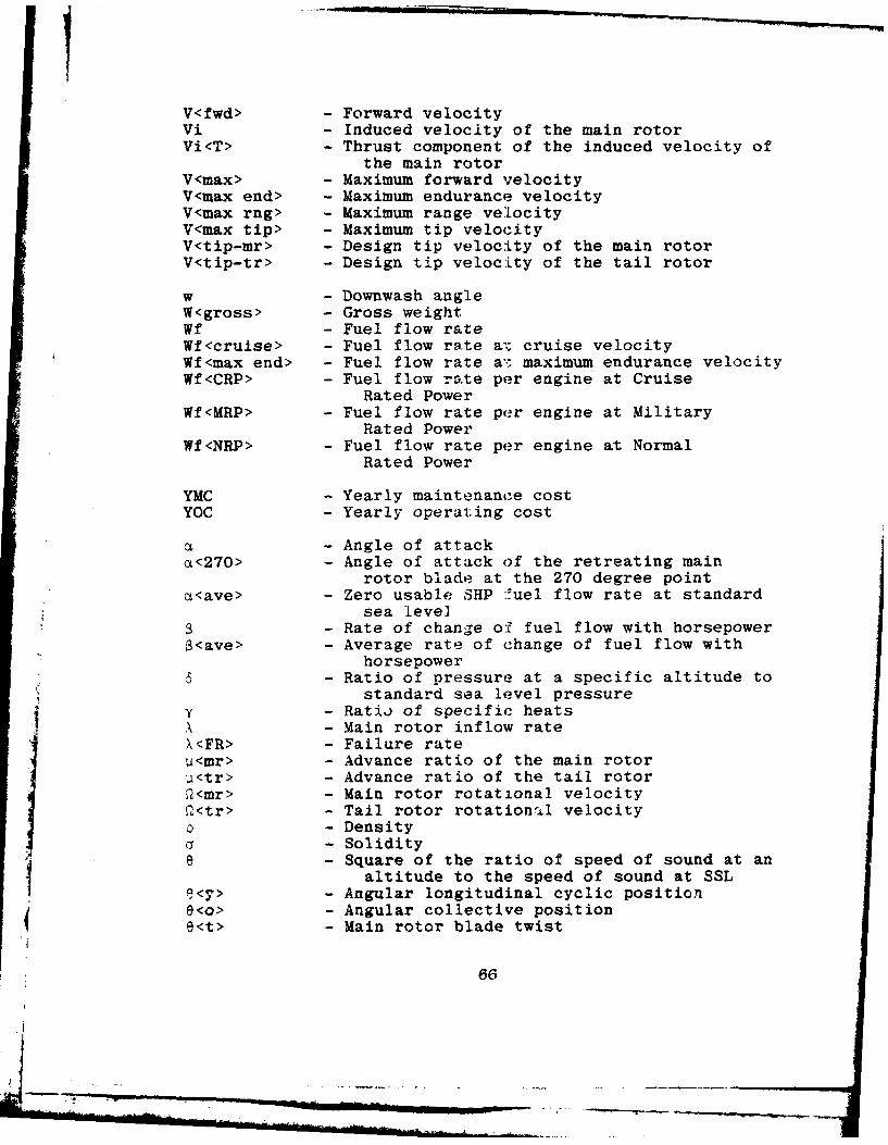
V<fwd> - Forward velocityVi - Induced velocity of the main rotorVi<T> - Thrust component of the induced velocity of

the main rotorV<max> - Maximum forward velocityV<max end> - Maximum endurance velocityV<max rng> - Maximum range velocityV<max tip> - Maximum tip velocityV<tip-mr> - Design tip velocity of the main rotorV<tip-tr> - Design tip velocity of the tail rotor

w - Downwash angleW<gross> - Gross weightWf - Fuel flow rateWf<cruise> - Fuel flow rate ai; cruise velocityWf<max end> - Fuel flow rate a-; maximum endurance velocityWf<CRP> - Fuel flow rate per engine at Cruise

Rated PowerWf<MRP> - Fuel flow rate per engine at Military

Rated PowerWf<NRP> - Fuel flow rate per engine at Normal

Rated Power

YMC - Yearly maintenance costYOC - Yearly operating cost

a- Angle of attacka<270> - Angle of attack of the retreating main

rotor blade at the 270 degree pointa<ave> - Zero usable SHP :fuel flow rate at standard

sea level- Rate of change of fuel flow with horsepower

3<ave> - Average rate of change of fuel flow withhorsepower

5 - Ratio of pressure at a specific altitude tostandard sea level pressure

y - Ratio of specific heatsX -Main rotor inflow rateX<FR> - Failure rate

- Advance ratio of the main rotor<tr> - Advance ratio of the tail rotor

-<mr> Main rotor rotational velocity-<tr> Tail rotor rotationU velocity- Density

5 - Soliditye - Square of the ratio of speed of sound at an

altitude to the speed of sound at SSLe<y> - Angular longitudinal cyclic position9<0> - Angular collective positione<t> - Main rotor blade twist

66

Appendix A-3

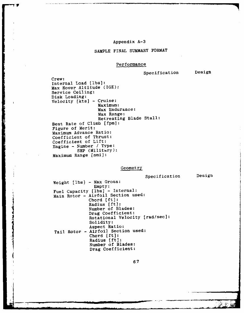
SAMPLE FINAL SUMMARY FORMAT

Performance

Specification Design

Crew:Internal Load [lbs]:Max Hover Altitude (IGE):

Service Ceiling:Disk Loading:Velocity [kts] - Cruise:

Maximum:Max Endurance:Max Range:Retreating Blade Stall:

Best Rate of Climb [fpm]:Figure of Merit:Maximum Advance Ratio:Coefficient of Thrust:Coefficient of Lift:Engine - Number / Tvpe:

SHP (Military):

Maximum Range [nmi]:

Geometry

Specification Design

Weight [lbs] - Max Gross:Empty:

Fuel Capacity [ibs] - Internal:Main Rotor - Airfoil Section used:

! Chord [ft]:Radius [ft]:Number of Blades:Drag Coefficient:Rotational Velocity [rad/sec]:Solidity:Aspect Ratio:

Tail Rotor - Airfoil Section used:Chord [ft]:Radius [ft]:Number of Blades:Drag Coefficient:

67

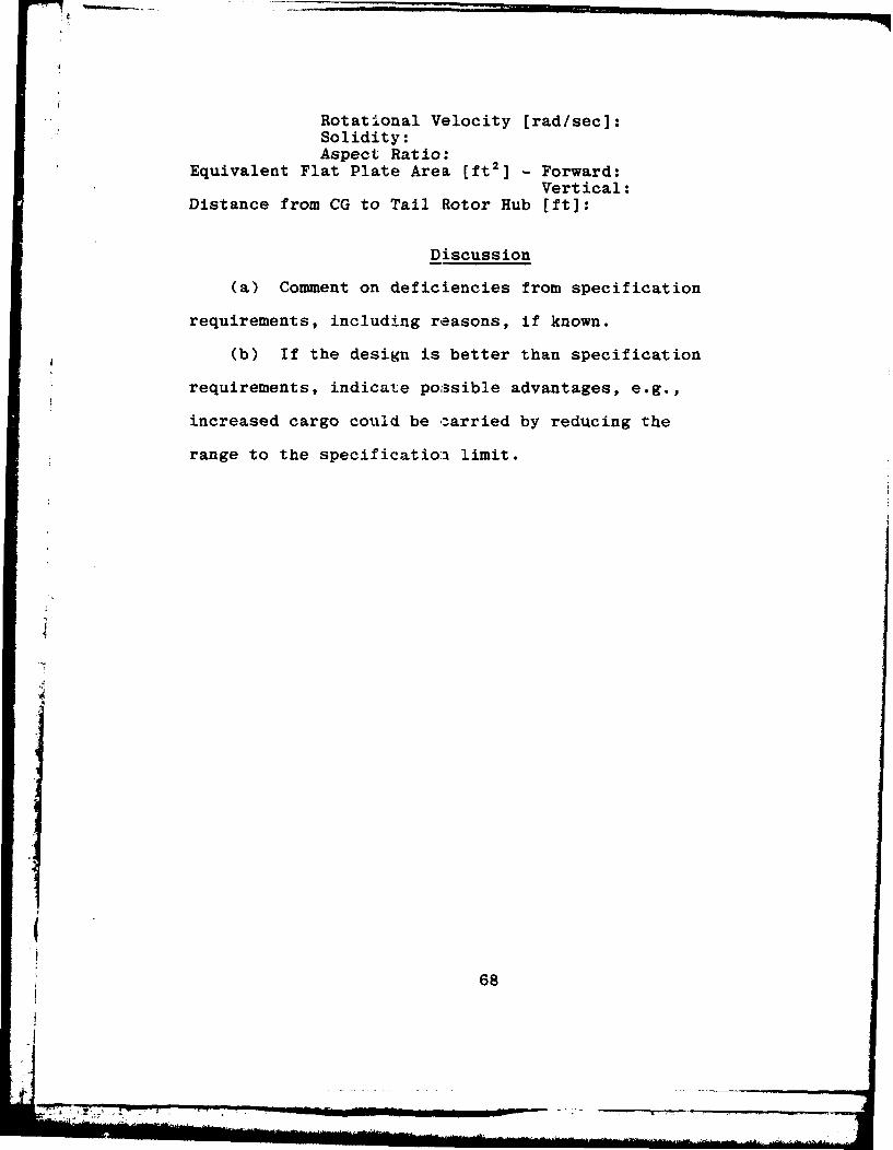
Rotational Velocity [rad/sec]:Solidity:Aspect Ratio:

Equivalent Flat Plate Area [ft 2 ] - Forward:Vertical:

Distance from CG to Tail Rotor Hub [ft]:

Discussion

(a) Comment on deficiencies from specification

requirements, including reasons, if known.

(b) If the design is better than specification

requirements, indicate po:ssible advantages, e.g.,

increased cargo could be carried by reducing the

range to the specificatio: limit.

(I

68

, .. . ... .. .._ _"_ _--_ _

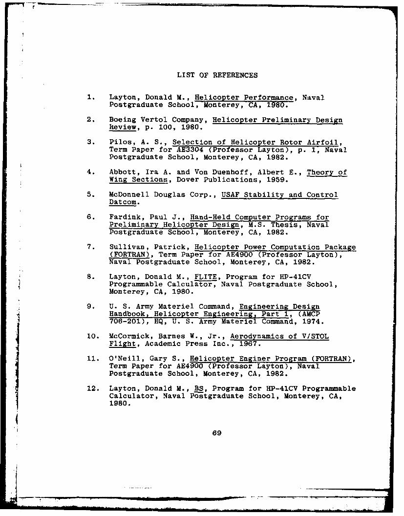
LIST OF REFERENCES

1. Layton, Donald M., Helicopter Performance, NavalPostgraduate School, Monterey, CA, 1980.

2. Boeing Vertol Company, Helicopter Preliminary DesignReview, p. 100, 1980.

3. Pilos, A. S., Selection of Helicopter Rotor Airfoil,Term Paper for AE3304 (Professor Layton), p. 1, NavalPostgraduate School, Monterey, CA, 1982.

4. Abbott, Ira A. and Von Duenhoff, Albert E., Theory ofWing Sections, Dover Publications, 1959.

5. McDonnell Douglas Corp., USAF Stability and ControlDatcom.

6. Fardink, Paul J., Hand-Held Computer Programs forPreliminary Helicopter Design, M.S. Thesis, NavalPostgraduate School, Monterey, CA, 1982.

7. Sullivan, Patrick, Helicopter Power Computation Package(FORTRAN), Term Paper for AE4900 (Professor Layton),Naval Postgraduate School, Monterey, CA, 1982.

8. Layton, Donald M., FLITE, Program for HP-41CVProgrammable Calculator, Naval Postgraduate School,Monterey, CA, 1980.

9. U. S. Army Materiel Command, Engineering DesignHandbook, Helicopter Engineering, Part 1, (AMCP706-201), HQ, U. S. Army Materiel Command, 1974.

10. McCormick, Barnes W., Jr., Aerodynamics of V/STOLFlight, Academic Press Inc., 1967.

11. O'Neill, Gary S., Helicopter Enginer Program (FORTRAN),Term Paper for AE4900 (Professor Layton), NavalPostgraduate School, Monterey, CA, 1982.

12. Layton, Donald M., BS, Program for HP-41CV ProgrammableCalculator, Naval Postgraduate School, Monterey, CA,1980.

669

BIBLIOGRAPHY

Barish, Norman N. and Kaplan, Seymour, Economic Analysis,McGraw-Hill Book Co., 1978.

English, John M. (Editor), Cost-Effectiveness, JohnWiley and Sons, Inc., 1968.

Haupt, Ulrich, Decision-making and Optimization in Air-craft Design, Naval Postgraduate School, Monterey, CA,1977.

Jones, J. Christopher, Design Methods, John Wiley andSons, Inc., 1970.

Morrison, Richard B. (Editor), Design Data for Aeronauticsand Astronautics, John Wiley and Sons, Inc., 1962.

Newman, Donald G., Engineering Economic Analysis,Engineering Press, 1976.

Pitts, G., Techniques in Engineering Design, John Wileyand Sons, Inc., 1973.

Saunders, George H., Dynamics of Helicopter Flight,John Wiley and Sons, Inc., 1975.

Thuesen, Halger G., Fabrycky, W. J., and Thuesen G. J.,Engineering Economy, 4th ed., Prentice-Hall, In.,1971.

Wood, Karl D., Aerospace Vehicle Design. Vol. I(Aircraft Design), 3d ed., Johnson Publishing Co.,1968.

70

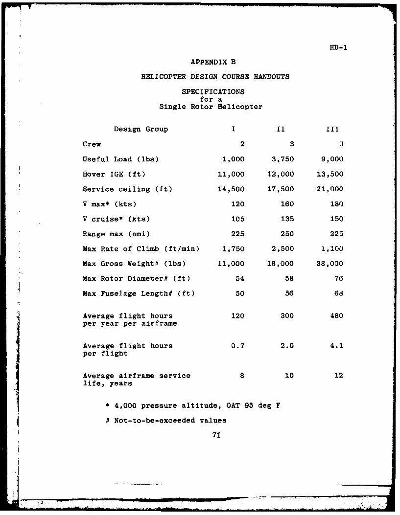
HD-i

APPENDIX B

HELICOPTER DESIGN COURSE HANDOUTS

SPECIFICATIONSfor a

Single Rotor Helicopter

Design Group I II III

Crew 2 3 3

Useful Load (lbs) 1,000 3,750 9,000

Hover IGE (ft) 11,000 12,000 13,500

Service ceiling (ft) 14,500 17,500 21,000

V max* (kts) 120 160 180

V cruise* (kts) 105 135 150

Range max (nmi) 225 250 225

Max Rate of Climb (ft/min) 1,750 2,500 1,100

Max Gross Weight# (lbs) 11,000 18,000 38,000

Max Rotor Diameter# (ft) 54 58 76

Max Fuselage Length# (ft) 50 56 68

Average flight hours 120 300 480per year per airframe

Average flight hours 0.7 2.0 4.1per flight

Average airframe service 8 10 12life, years

4,000 pressure altitude, OAT 95 deg F

# Not-to-be-exceeded values

71

R

HD- 2

Z32

~28

024_

00

16

8

0 2 4 6 8 10 12 14 16 I8MANUFACTURERS EMPTY WEIGHT

(1,000 LBS)

72

kID- 3

.. ......

0 0 0

o9NIaV-I osia73

HD- 4

.10

0

47

HD-5

.03.~.~1.4

1.2 .. .

J02 10

.... .........

.......1 ................

02 2.. ..... 6 .. .. 0

ANGLE OF ATTACK (DEG)

75

HD-6

HELICOPTER DESIGN COURSE HANDOUT

Weight Estimation

Main Rotor -

W<blades> - 0.06 * W<empty> *R<mr> 0- * a<mr 0 .3 3

W<hub> = 0.0135 * W<empty> *R<mr> 0.2

W<mr> = W<blades> + W<hub>

Propulsion -

W<prp> =1.2 * SHP<req>

Fuselage-

W<fu> =0.21 * W<empty>

Controls-

W<ctl> =0.06 *W<empty>

Electrical -

W<el> = 0.06 *W<empty>

Fixed Equipment-

W<fe> = 0.28 *Wcempty>

Empty Weight (second cut)-

W<empty> = W<mr> + W<prp> + W<fu> + W<ctl> + W<el> +1 W<fe>

Gross Weight (second cut) -

W<gross> =W<empty> + W<fuel> + W<load>

76

W r-..,

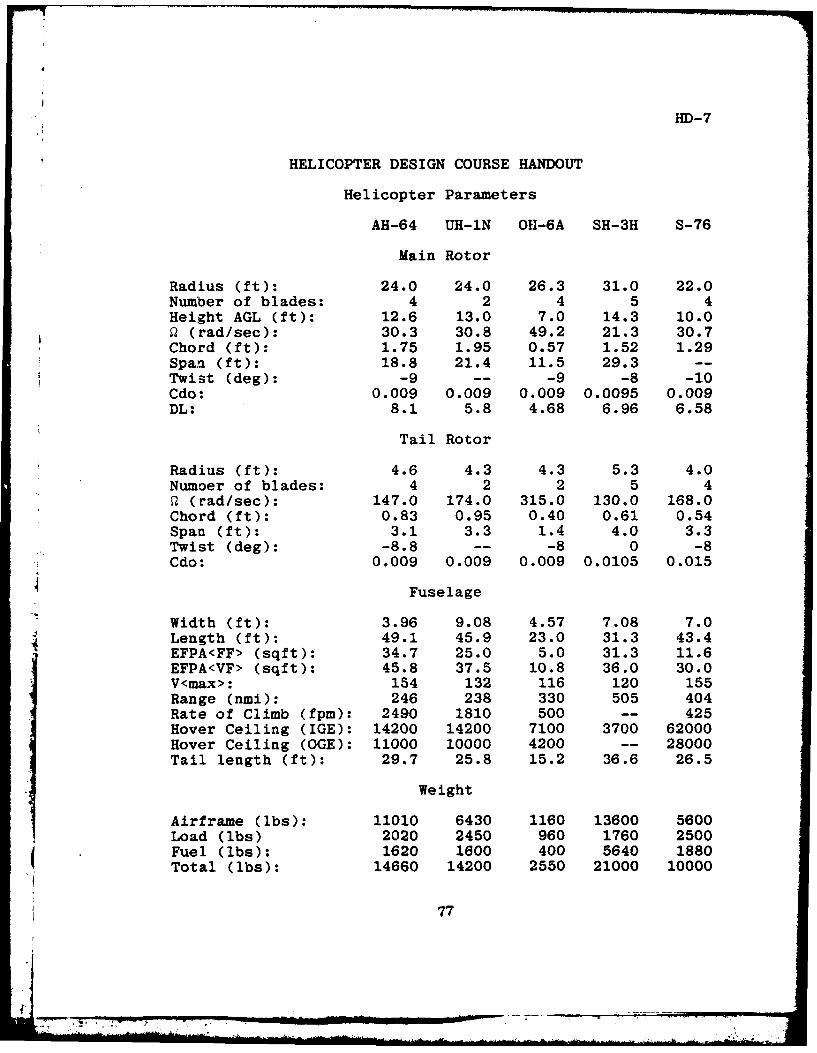
liD-7


Helicopter Parameters

AH-64 UH-1N OR-6A SH-3H S-76

Main Rotor

Radius (ft): 24.0 24.0 26.3 31.0 22.0Number of blades: 4 2 4 5 4Height AGL (ft): 12.6 13.0 7.0 14.3 10.0Q (rad/sec): 30.3 30.8 49.2 21.3 30.7Chord (ft): 1.75 1.95 0.57 1.52 1.29Span (ft): 18.8 21.4 11.5 29.3 --Twist (deg): -9 -- -9 -8 -10Cdo: 0.009 0.009 0.009 0.0095 0.009DL: 8.1 5.8 4.68 6.96 6.58

Tail Rotor

Radius (ft): 4.6 4.3 4.3 5.3 4.0Numoer of blades: 4 2 2 5 49 (rad/sec): 147.0 174.0 315.0 130.0 168.0Chord (ft): 0.83 0.95 0.40 0.61 0.54Span (ft): 3.1 3.3 1.4 4.0 3.3Twist (deg): -8.8 -- -8 0 -8Cdo: 0.009 0.009 0.009 0.0105 0.015

Fuselage

Width (ft): 3.96 9.08 4.57 7.08 7.0Length (ft): 49.1 45.9 23.0 31.3 43.4EFPA<FF> (sqft): 34.7 25.0 5.0 31.3 11.6EFPA<VF> (sqft): 45.8 37.5 10.8 36.0 30.0V<max>: 154 132 116 120 155Range (nmi): 246 238 330 505 404Rate of Climb (fpm): 2490 1810 500 -- 425Hover Ceiling (IGE): 14200 14200 7100 3700 62000Hover Ceiling (OGE): 11000 10000 4200 -- 28000Tail length (ft): 29.7 25.8 15.2 36.6 26.5

Weight

Airframe (lbs): 11010 6430 1160 13600 5600Load (lbs) 2020 2450 960 1760 2500Fuel (lbs): 1620 1600 400 5640 1880Total (lbs): 14660 14200 2550 21000 10000

77

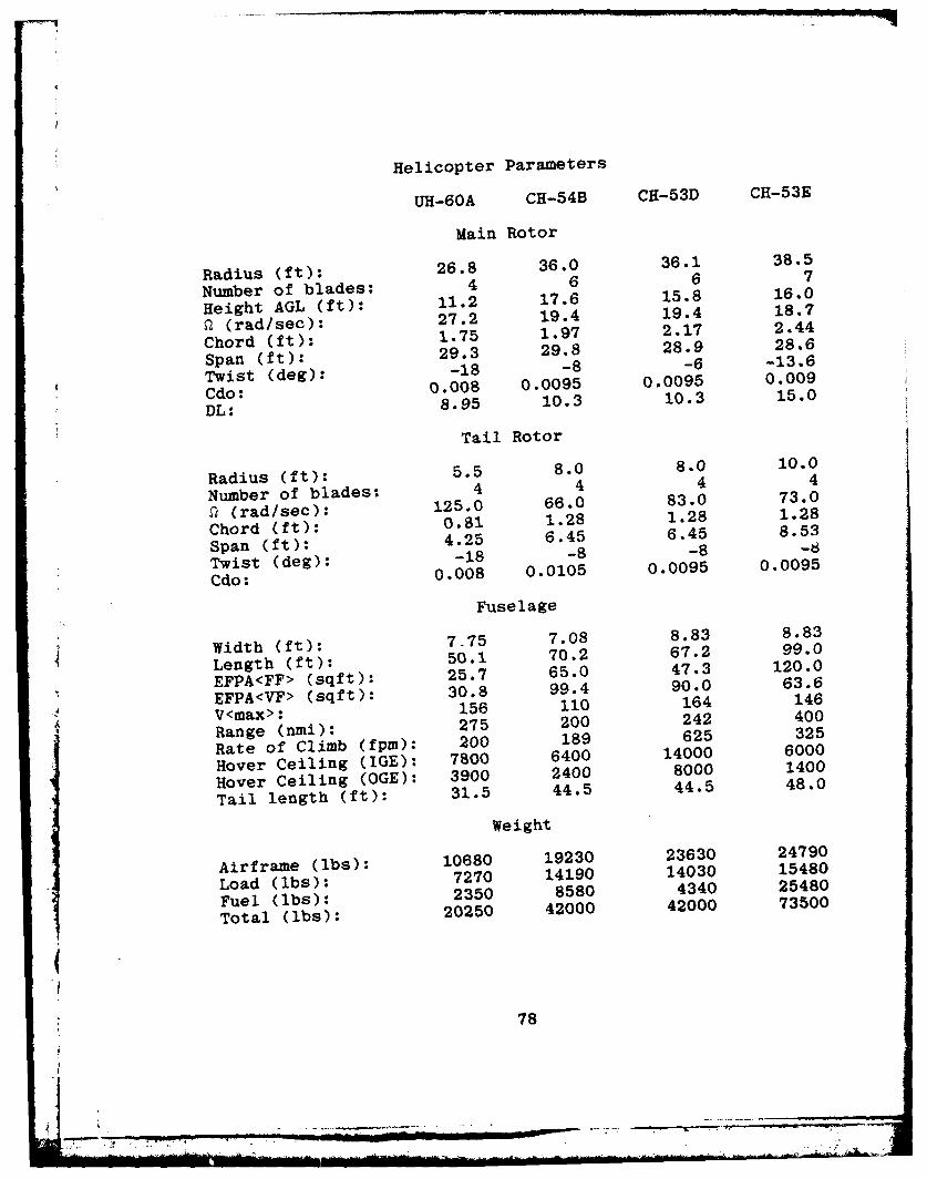
Helicopter Parameters

UH-60A CH-54B CH-53D CH-53E

Main Rotor

Radius (ft): 26.8 36.0 36.1 38.5

Number of blades: 4 6 6 7

Height AGL (ft): 11.2 17.6 15.8 16.0

Q (rad/seC): 27.2 19.4 19.4 18.7

Chord (ft): 1.75 1.97 2.17 2.44

Span (ft): 29.3 29.8 28.9 28.6

Twist (deg): -18 -8 -6 -13.6

Odo: 0.008 0.0095 0.0095 0.009

DL: 8.95 10.3 10.3 15.0

Tail Rotor

Radius (ft): 5.5 8.0 8.0 10.0

Number of blades: 4 4 4 4

02 (rad/seC): 125.0 66.0 83.0 73.0

Chord (ft): 0.81 1.28 1.28 1.28

Span (ft): 4.25 6.45 6.45 8.53

Twist (deg): -18 -8 -8 -8

Cdo: 0.008 0.0105 0.0095 0.0095

Fuselage

Width (ft): 7-75 7.08 8.83 8.83

Length (ft): 50.1 70.2 67.2 99.0

EFPA<FF> (sqft): 25.7 65.0 47.3 120.0

EFPA<VF> (sqft): 30.8 99.4 90.0 63.6

V<max>: 156 110 164 146

Range (nmi): 275 200 242 400

Rate of Climb (fpmn): 200 189 625 325

Hover Ceiling (IGE): 7800 6400 14000 6000

Hover Ceiling (OGE): 3900 2400 8000 1400

Tail length (ft): 31.5 44.5 44.5 48.0

Weight

Airframe (ibs): 10680 19230 23630 24790

Load (lbs): 7270 14190 14030 15480

Fuel (lbs): 2350 8580 4340 25480

Total (lbs): 20250 42000 42000 73500

78

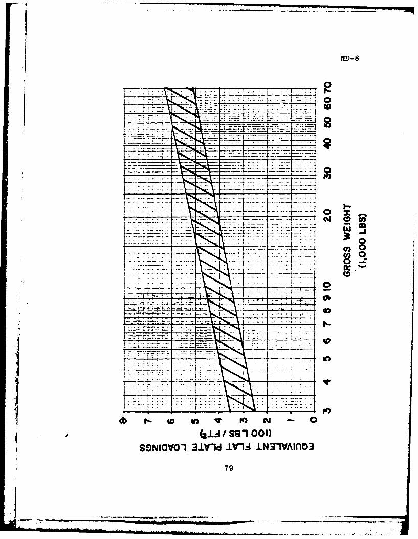
HD-8

- 7 40-77

- -- ~-)

.7 7 -

77_ _-

(2- -se--100 1)

SNOI 1-.d ------ CDi~i

* ~- -..- .- - - '~1:~79 -

I'D-9


Tail Geometry Factors

The following factors are based on analysis of several

typical helicopters.

Generalized Data

Tail radius (ft): R<tr> = 1.3 * F W<gross> / 1000

Tail RPM: Q<tr> = 4.5 * Main rotor RPM

Tail Cdo: Cdo<tr> = 0.0138 * Main rotor Cdo

Group: I II III

Number of blades: 2 3 - 4 4 - 7

80

80

HD-10

.70

.60-

i0 2 4 6 8

ANGLE OF ATTACK (DEG)

81

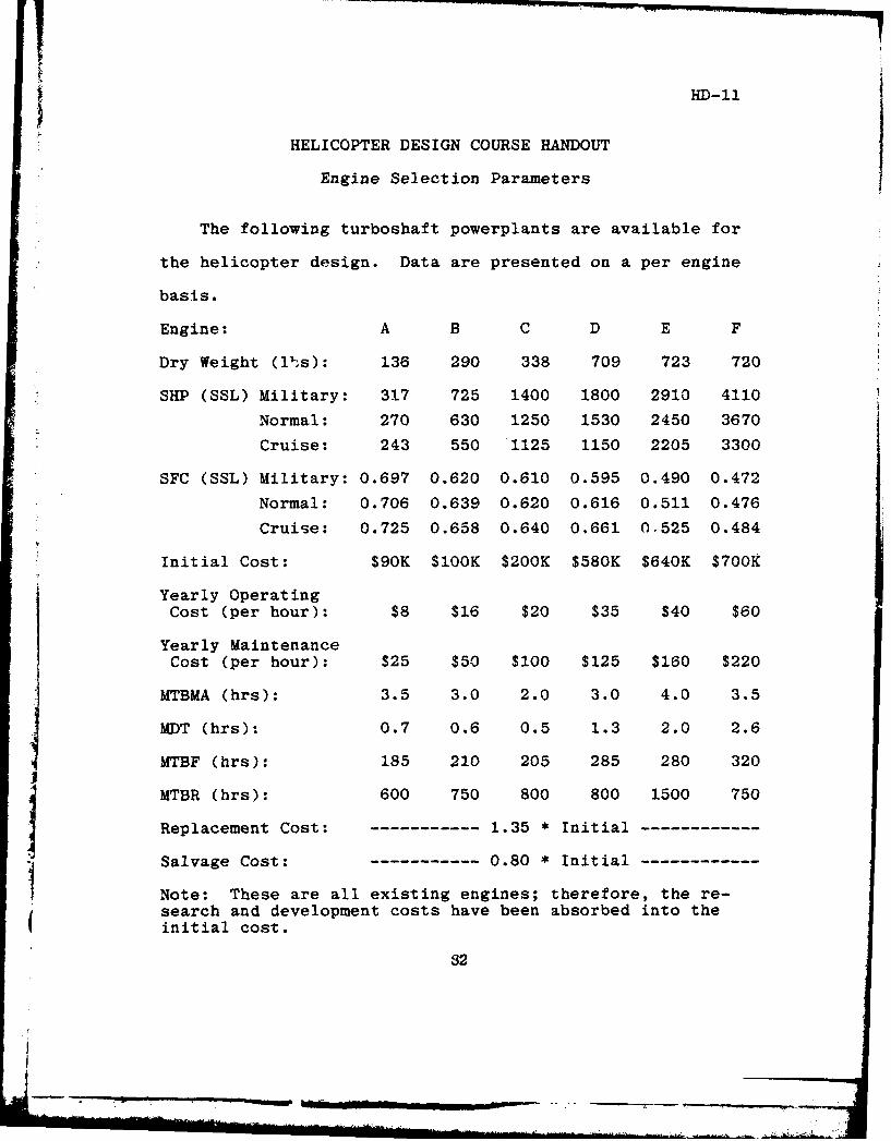
HD-11


Engine Selection Parameters

The following turboshaft powerplants are available for

the helicopter design. Data are presented on a per engine

basis.

Engine: A B C D E F

Dry Weight (lhs): 136 290 338 709 723 720

SHP (SSL) Military: 317 725 1400 1800 2910 4110

Normal: 270 630 1250 1530 2450 3670

Cruise: 243 550 1125 1150 2205 3300

SFC (SSL) Military: 0.697 0.620 0.610 0.595 0.490 0.472

Normal: 0.706 0.639 0.620 0.616 0.511 0.476

Cruise: 0.725 0.658 0.640 0.661 0.525 0.484

Initial Cost: $90K $100K $200K $580K $640K $700K

Yearly OperatingCost (per hour): $8 $16 $20 $35 $40 $60

Yearly MaintenanceCost (per hour): $25 $50 $100 $125 $160 $220

MTBMA (hrs): 3.5 3.0 2.0 3.0 4.0 3.5

MDT (hrs): 0.7 0.6 0.5 1.3 2.0 2.6

MTBF (hrs): 185 210 205 285 280 320

MTBR (hrs): 600 750 800 800 1500 750

Replacement Cost: ----------- 1.35 * Initial------------

Salvage Cost: ----------- 0.80 * Initial------------

Note: These are all existing engines; therefore, the re-search and development costs have been absorbed into theinitial cost.

32

• ~ ~ ~ ~ ~ ~ ~ ~ ~ ~ ~ ~ .. .......... I , JL I . . - .. . - ..

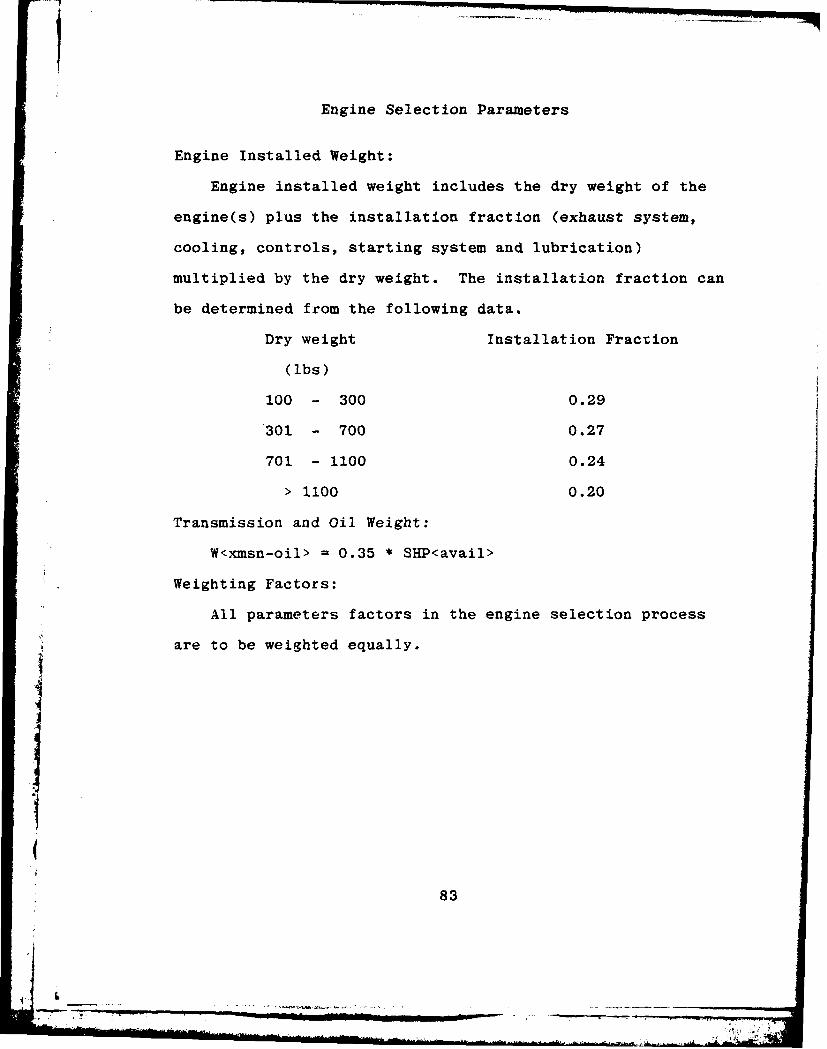
Engine Selection Parameters

Engine Installed Weight:

Engine installed weight includes the dry weight of the

engine(s) plus the installation fraction (exhaust system,

cooling, controls, starting system and lubrication)

multiplied by the dry weight. The installation fraction can

be determined from the following data.

Dry weight Installation Fraction

(lbs)

100 - 300 0.29

301 - 700 0.27

701 - 1100 0.24

> 1100 0.20

Transmission and Oil Weight:

W<xmsn-oil> = 0.35 * SHP<avail>

Weighting Factors:

All parameters factors in the engine selection process

are to be weighted equally.

83

I.1

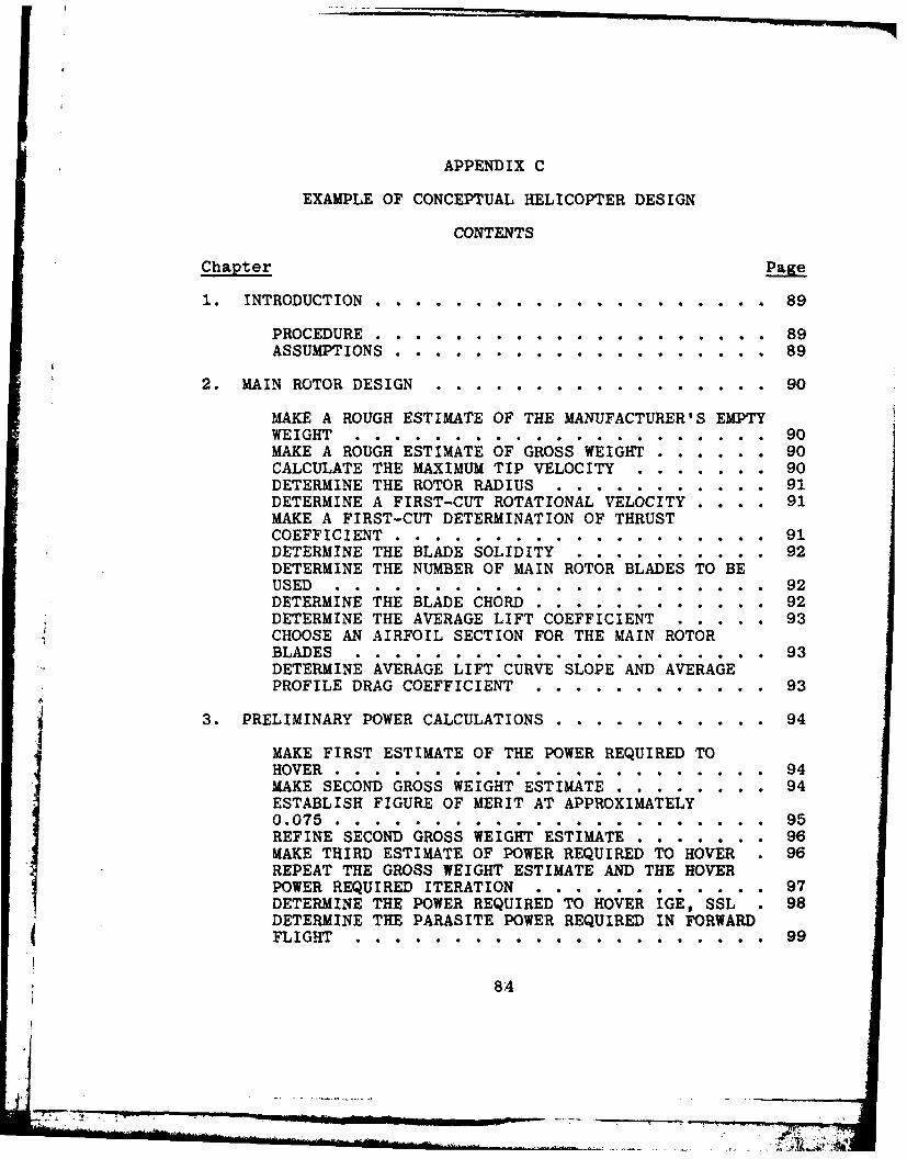
APPENDIX C

EXAMPLE OF CONCEPTUAL HELICOPTER DESIGN

CONTENTS

Chapter Page

1. INTRODUCTION . . ................. . . . . 89

PROCEDURE . . . . . . . . ....... . . . . . 89ASSUMPTIONS ....... .................. . 89

2. MAIN ROTOR DESIGN ...... ................. 90

MAKE A ROUGH ESTIMATE OF THE MANUFACTURER'S EMPTYWEIGHT ........ ................ 90MAKE A ROUGH ESTIMATE OF GROSS WEIGHT . . . . . 90CALCULATE THE MAXIMUM TIP VELOCITY ........ . 90DETERMINE THE ROTOR RADIUS .. ......... 91DETERMINE A FIRST-CUT ROTATIONAL VELOCITY .... 91MAKE A FIRST-CUT DETERMINATION OF THRUSTCOEFFICIENT .......... ............ 91DETERMINE THE BLADE SOLIDITY"..... . 92DETERMINE THE NUMBER OF MAIN ROTOR BLADES TO'BEUSED .......... .................. 92DETERMINE THE BLADE CHORD.-. . .. ...... .. 92DETERMINE THE AVERAGE LIFT COEFFICIENT . . . . . 93CHOOSE AN AIRFOIL SECTION FOR THE MAIN ROTORBLADES ......... ................ . . 93DETERMINE AVERAGE LIFT CURVE SLOPE AND AVERAGEPROFILE DRAG COEFFICIENT ... ............ 93

3. PRELIMINARY POWER CALCULATIONS ... ........... . 94

MAKE FIRST ESTIMATE OF THE POWER REQUIRED TOHOVER ................. ........ 94MAKE SECOND GROSS WEIGHT ESTIMATE .. ......... 94ESTABLISH FIGURE OF MERIT AT APPROXIMATELY0.075 ............ .. ...... 95REFINE SECOND GROSS WEIGHT ESTIMATE. 96MAKE THIRD ESTIMATE OF POWER REQUIRED TO HOVER 96REPEAT THE GROSS WEIGHT ESTIMATE AND THE HOVERPOWER REQUIRED ITERATION . ...... 97DETERMINE THE POWER REQUIRED'TO HOVEi IGE, SSL • 98DETERMINE THE PARASITE POWER REQUIRED IN FORWARDFLIGHT . . ......... . . . . . . . . . . . . 99

84

7- . . ..

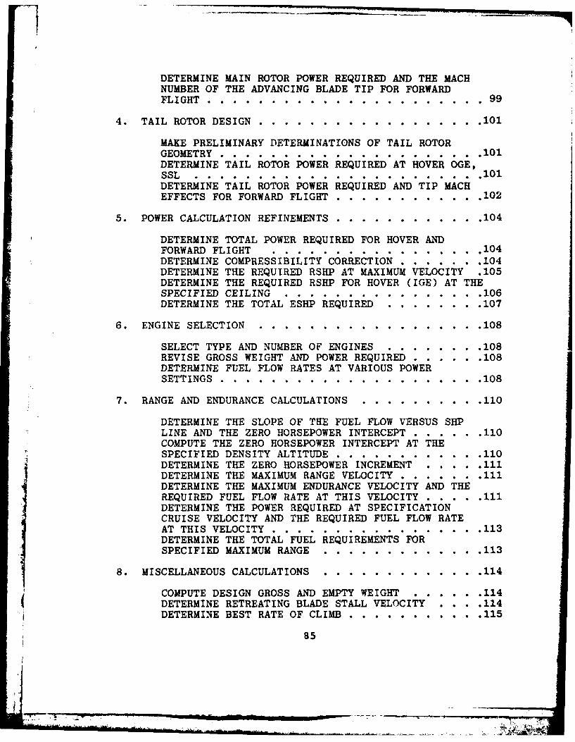
DETERMINE MAIN ROTOR POWER REQUIRED AND THE MACHNUMBER OF THE ADVANCING BLADE TIP FOR FORWARDFLIGHT ......................... 99

4. TAIL ROTOR DESIGN ........... . . . ........ 1 01

MAKE PRELIMINARY DETERMINATIONS OF TAIL ROTORGEOMETRY ... ......... . . . . ...... .101DETERMINE TAIL ROTOR POWER REQUIRED AT HOVER OGE,SSL ......... .. 101DETERMINE TAIL ROTOR POWER REQUIRED'AND'TIP'MACHEFFECTS FOR FORWARD FLIGHT ..... ............ 102

5. POWER CALCULATION REFINEMENTS ........... . . 104

DETERMINE TOTAL POWER REQUIRED FOR HOVER ANDFORWARD FLIGHT ................ . . . . . . 104DETERMINE COMPRESSIBILITY CORRECTION . . . . . . .104DETERMINE THE REQUIRED RSHP AT MAXIMUM VELOCITY .105DETERMINE THE REQUIRED RSHP FOR HOVER (IGE) AT THESPECIFIED CEILING ................... 106DETERMINE THE TOTAL ESHP REQUIRED ......... 107

6. ENGINE SELECTION . . . . ................. 108

SELECT TYPE AND NUMBER OF ENGINES .. ........ .108REVISE GROSS WEIGHT AND POWER REQUIRED ........ 108DETERMINE FUEL FLOW RATES AT VARIOUS POWERSETTINGS ......... ..................... 108

7. RANGE AND ENDURANCE CALCULATIONS .... ......... . 110

DETERMINE THE SLOPE OF THE FUEL FLOW VERSUS SHPLINE AND THE ZERO HORSEPOWER INTERCEPT ... ...... 110COMPUTE THE ZERO HORSEPOWER INTERCEPT AT THESPECIFIED DENSITY ALTITUDE ... ........ 110DETERMINE THE ZERO HORSEPOWER INCREM.ENT . .. . .ilDETERMINE THE MAXIMUM RANGE VELOCITY. ........ .111DETERMINE THE MAXIMUM ENDURANCE VELOCITY AND THEREQUIRED FUEL FLOW RATE AT THIS VELOCITY ...... .111DETERMINE THE POWER REQUIRED AT SPECIFICATIONCRUISE VELOCITY AND THE REQUIRED FUEL FLOW RATEAT THIS VELOCITY ............... . _ 113DETERMINE THE TOTAL FUEL REQUIREMENTS FORSPECIFIED MAXIMUM RANGE ..... ............. 113

8. MISCELLANEOUS CALCULATIONS ..... ............. 114

COMPUTE DESIGN GROSS AND EMPTY WEIGHT . . . . . . 114DETERMINE RETREATING BLADE STALL VELOCITY . . . . 114DETERMINE BEST RATE OF CLIMB . . . . . . . . . . . 115

85

COMPUTE MAXIMUM HOVER ALTITUDE (IGE) . . . . . . 116

COMPUTE SERVICE CEILING . . . . . . . . . . . . 117

9. FINAL CHECK. ......... . . . . . . . . . . . . 119

MAKE FINAL CHECK FOR COMPLIANCE WITHSPECIFICATIONS . . . . . . . . . .. .. .. ... 119

LIST OF REFERENCES . . . . . . . .. .. .. ... ... 121

86

LIST OF TABLES

Table page

1. Weight Estimation Table . . . . . . . . . . . . . 95

2. Main Rotor Power Profile . . . . . . . . . ... 100

3. Tail Rotor Power Profile . . . . . . . . .. .. 103

4. Total Rotor Power Profile . . . . . . . . . .. . 106

5. Engine Selection Criteria . . . . . . . . . . . . 109

6. Best Rate of Climb Iterations . .. .. .. . .. 116

7. Maximum Hover Altitude (IGE) Iterations . . .. . 117

8. Service Ceiling Iterations .. .......... . . 118

9. Final Summary .................... . . . .. 119

87

li ' . . . . ... . .. . ..... .. ..

4i

LIST OF FIGURES

Figure page

1. Maximum Range Velocity . . . . . . . . . . . . . . 111

2. Maximum Endurance Velocity...... . . . . . . 112

888

Chapter 1

INTRODUCTION

1.1 PROCEDURE

This design example is for the conceptual design of a

single main rotor, utility helicopter. The design method

I 1 utilizes closed form formulas and symbology obtained from

the design manual [Ref. 1] written for use in AE4306. Italso uses approximations from historical data given in the

various AE4306 handouts (see Appendix B). This example was

written using the specifications contained in IID-1 for

Design Group I.

1.2 ASSUMPTIONS

There have been several assumptions made in the design

process as per the instructions given in Reference 1. These

assumptions are mentioned as they occur in the design

process.

I

89

V.

Chapter 2

MAIN ROTOR DESIGN

2.1 MAKE A ROUGH ESTIMATE OF THE MANUFACTURER'S EMPTY

WEIGHT.

The specification maximum gross weight from HD-I is

11,000 lbs. The graph of historical weight ratios (HD-2)

indicates that the manufacturer's empty weight is 60% of

the gross weight. Therefore, the first estimate of

manufacturer's empty weight is 6,600 lbs.

2.2 MAKE A ROUGH ESTIMATE OF GROSS WEIGHT.

An estimated gross weight which is 80% of the specifi-

cation value of gross weight should be used. The specifica-

tion value of gross weight from HD-i is 11,000 lbs.

W<gross> = 0.8 * 11,000. = 8,800. lbs

2.3 CALCULATE THE MAXIMUM TIP VELOCITY.

At a hover, the main rotor tip Mach number should not

exceed 0.65; therefore, M<max tip-mr> = 0.65. At standard

sea level the value of the ratio of specific heats is 1.4,

the local gravitational constant is 32.2 ft/sec 2 , the gas

cons.ant is 53.3 and the temperature is 518.688 degrees R.

a= Vy* g*R*T'

1.4 * 32.2 * 53.3 * 518.688 1= 1116.3713 ft/sec

V<max tip-mr> = M<max tip-mr> * a

= 0.65 * 1116.3713 - 725.6413 ft/sec

90

2.4 DETERMINE THE ROTOR RADIUS.

Using HD-3 a disk loading value of 6.0 was chosen. The

maximum value of main rotor radius given in HD-1 is 27 ft.

R<mr> = . W<gross> / (DL * ir)

= 8800.0 / (6.0 * 3.1416) 21.6068 ft

2.5 DETERMINE A FIRST-CUT ROTATIONAL VELOCITY.

The maximum tip velocity is 725.6413 ft/sec from Step

2.3. The specification maximum forward velocity is 202.6667

ft/sec from HD-I. The design rotor radius is 21.6068 ft

from Step 2.4.

Q<mr-max> = V<max tip-mr> / R<mr>

- 725.6413 / 21.6068 = 33.5839 rad/sec

2.6 MAKE A FIRST-CUT DETERMINATION OF THRUST COEFFICIENT.

The specification density altitude is 7122.1.3 ft from

jHD-I, at which the density is 0.0019196 slugs/ft. The

rotational velocity is 33.5839 rad/sec from Step 2,5.

_Thrust equals the value of gross weight found in S.ep 2.2.

Using the main rotor radius found in Step 2.4, the main

rotor area is 1466.6645 ft2 .

V<tip-mr> = Q<mr> * R<mr>

- 33.5839 * 21.6068 = 725.6413 ft/sec

C<thrust-mr> - T<mr> / [A<mr> *p * V<tip-mr>2]

= 8800.00/ [1466.6645*0.0019196*(725.6413)2] - 0.0059

91

2.7 DETERMINE THE BLADE SOLIDITY.

The maximum forward velocity is 202.6667 ft/sec and the

tip velocity is 725.6413 ft/sec from Step 2.6. Using the

maximum advance ratio and HD-4, the blade loading is 0.1065.

u<mr-max> = V<max> / V<tip-mr>

= 202.6667 / 725.6413 = 0.2793

a<mr> = C<thrust-mr> / BL

= 0.0059 / 0.1065 = 0.0554

2.8 DETERMINE THE NUMBER OF MAIN ROTOR BLADES TO BE USED.

Four rotor blades will be used. (Discuss reasons.)

2.9 DETERMINE THE BLADE CHORD.

The solidity is 0,0554 from Step 2.7. The number of

blades (Step 2.8) is 4 and the rotor radius (Step 2.4) is

21.6068 ft.

c<mr> = (a<mr> * * R<mr>) / b<mr>

= (0.0554 * 3.1416 * 21.6068) / 4 = 0.9401 ft

AR<mr>= R<mr> / c<mr> = 21.6068 / 0.9401 = 22.9827

Since the aspect ratio was not within the limits of 15 to

20, the rotational velocity (Step 2.5) was reduced to 31.00

rad/sec. Steps 2.6 and 2.7 were recalculated with the

following results.

l<mr>: 31.00 rad/sec V<tip-mr>: 669.8108 ft/sec

C<thrust-mr>: 0.0070 P<mr>: 0.3026

BL: 0.1038 U<mr>: 0.0674

%<mr>: 1.1444 ft AR<mr>: 18.8803

92

4. ________________________________________________

.. . i-- -

i ' i -i I I i .. . . . . . ... ..- .-- ,.-,--;

2.10 DETERMINE THE AVERAGE LIFT COEFFICIENT.

The thrust coefficient is 0.0070 from Step 2.10. The

solidity is 0.0674 from Step 2.10

C<lift> = ( 6 * C<thrust-mr> ) / ,<mr>

= ( 6 * 0.0070 ) / 0.0674 - 0.6231

2.11 CHOOSE AN AIRFOIL SECTION FOR THE MAIN ROTOR BLADES.

The selected airfoil section is airfoil "A" from HD-5.

(Discuss reasons.)

2.12 DETERMINE AVERAGE LIFT CURVE SLOPE AND AVERAGE

PROFILE DRAG COEFFICIENT.

From HD-5, the profile drag coefficient for airfoil "A"

is 0.010 and the lift curve slope (CL a ) is 6.4458 per

radian.

93

Chapter 3

PRELIMINARY POWER CALCULATIONS

3.1 MAKE FIRST ESTIMATE OF THE POWER REQUIRED TO HOVER.

The HP-41CV program entitled HOVER (Ref. 3] was used to

compute these values. The current value of all design

parameters are listed below.

DL: 6.00 W<gross>: 8800.00 lbs

R<mr>: 21.61 ft 2<mr>: 31.00 rad/sec

V<tip>: 669.81 ft/sec C<thrust>: 0.0070

<mr>: 0.3026 BL: 0.1038

<mr>: 0.0674 b<mr>: 4

c<mr>: 1.1444 ft AR<mr>: 18.88

C<lift>: 0.6231 Cdo<mr>: 0.0100

DA: 0.00

Pi<mr-TL>: 583.91 hp

Po<mr>: 160.56 hp

PT<mr-hover>: 744.48 hp

3.2 MAKE SECOND GROSS WEIGHT ESTIMATE.- Using HD-3, the first gross weight estimate used in the

main rotor design process was refined. The useful load was

computed using 200 lbs per crewmember. Table 1 shows the

result of the second gross weight estimate.

94

77 7,

TABLE 1

Weight Estimation Table

------------ ITERATION-------------FIRST SECOND THIRD FOURTH

SOLIDITY: - 0.0674 0.0674 0.0745RADIUS: - 21.6068 21.6068 20.7192TOTAL POWER: - 744.4755 734.3833 681.3628

ROTOR-LLADES: - 555.89 488.44 444.46HUB/HINGES: - 323.90 284.59 250.34TOTAL: - 879.79 773.03 694.80

PROPULSION: - 893.37 881.26 817.64FUSELAGE: - 1386.00 1217.82 109S).28FLIGHT CONTROLS: - 396.00 347.96 311.51ELECTRICAL: - 396.00 347.96 311.51FIXED EQUIPMENT: - 1848.00 1623.76 1453.70

EMPTY: 6600.00 5799.16 5191.80 4679.43

FUEL: - 1500.00 1500.00 1500.00USEFUL LOAD: - 1400.00 1406.00 1400.00

GROSS: 8800.00 8699.16 8091.80 7579.43

3.3 ESTABLISH FIGURE OF MERIT AT APPROXIMATELY 0.075.

The induced power from Step 3.1 was between 70 to 80% of

the total power from Step 3.1. In order to keep the same

radius, the disk loading was reduced to 5.93 (see Step 2.4).

The thrust coefficient (Step 2.6), the solidity (Step 2.7),

the chord (Step 2.9), the aspect ratio (Step 2.9), and the

lift coefficient (Step 2.10) were adjusted and the hover

power was recalculated (Step 3.1) using the second gross

weight estimate with the following results.

95

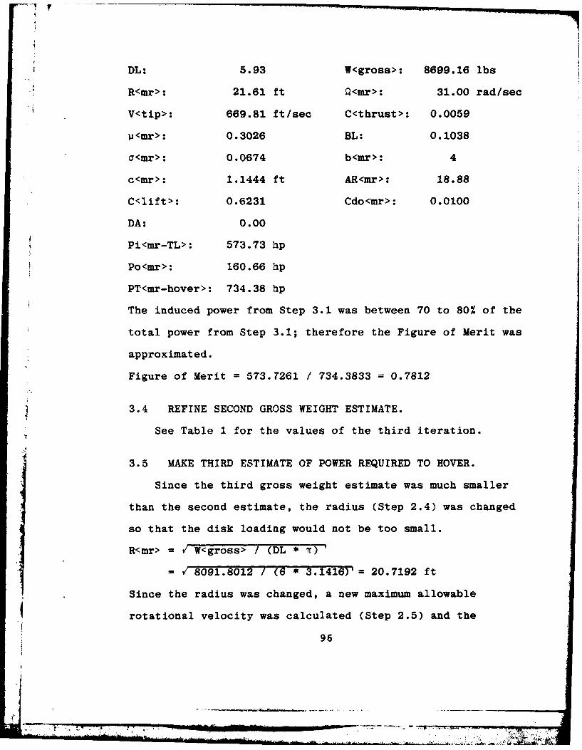
DL: 5.93 W<gross>: 8699.16 lbs

R<mr>: 21.61 ft s<mr>: 31.00 rad/sec


u<mr>: 0.3026 BL: 0.1038

a<mr>: 0.0674 b<mr>: 4

c<mr>: 1.1444 ft AR<mr>: 18.88

C<lift>: 0.6231 Cdo<mr>: 0.0100

DA: 0.00


Po<mr>: 160.66 hp


The induced power from Step 3.1 was between 70 to 80% of the

total power from Step 3.1; therefore the Figure of Merit was

approximated.

Figure of Merit = 573.7261 / 734.3833 = 0.7812

3.4 REFINE SECOND GROSS WEIGHT ESTIMATE.

See Table 1 for the values of the third iteration.

3.5 MAKE THIRD ESTIMATE OF POWER REQUIRED TO HOVER.

Since the third gross weight estimate was much smaller

than the second estimate, the radius (Step 2.4) was changed

so that the disk loading would not be too small.

R<mr> = W<gross> / (DL * 7)"

= 8091.8012 / (6 * 3.1416)' = 20.7192 ft

Since the radius was changed, a new maximum allowable

rotational velocity was calculated (Step 2.5) and the

96

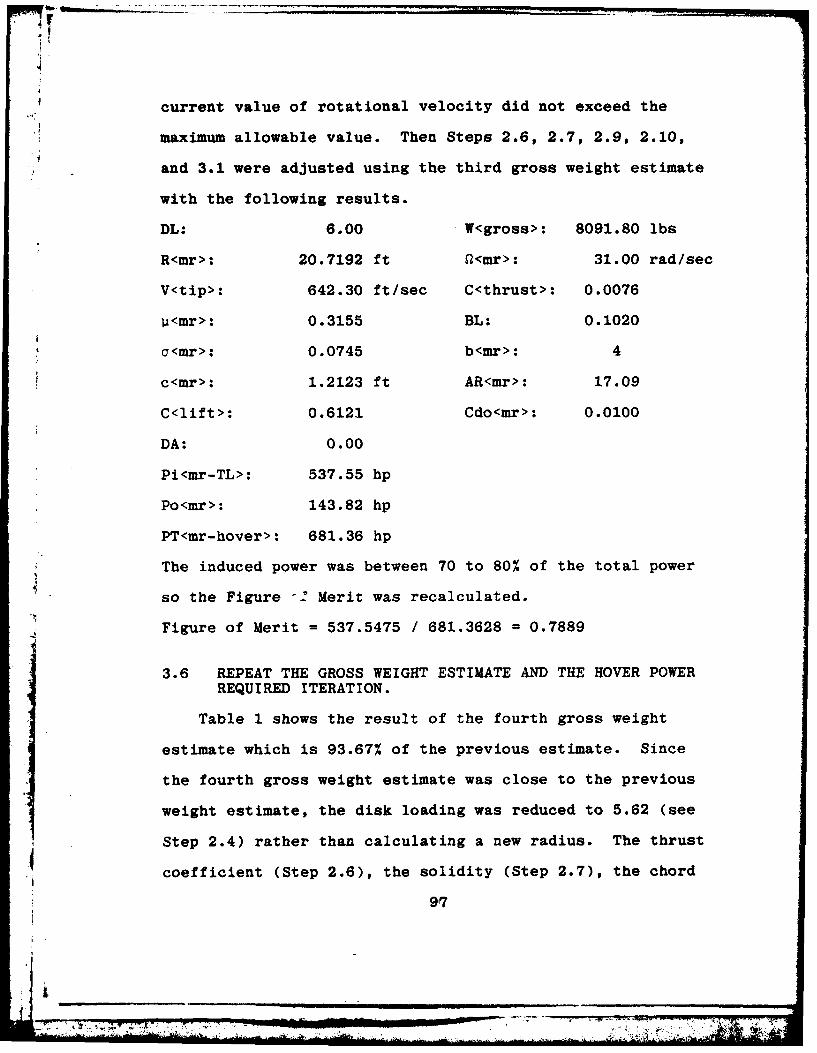
low.

current value of rotational velocity did not exceed the

maximum allowable value. Then Steps 2.6, 2.7, 2.9, 2.10,

and 3.1 were adjusted using the third gross weight estimate

with the following results.

DL: 6.00 W<gross>: 8091.80 lbs

R<mr>: 20.7192 ft R<mr>: 31.00 rad/sec


u<mr>: 0.3155 BL: 0.1020

a<mr>: 0.0745 b<mr>: 4

c<mr>: 1.2123 ft AR<mr>: 17.09

C<lift>: 0.6121 Cdo<mr>: 0.0100

DA: 0.00


Po<mr>: 143.82 hp


The induced power was between 70 to 80% of the total power

so the Figure -Z Merit was recalculated.

Figure of Merit = 537.5475 / 681.3628 = 0.7889

3.6 REPEAT THE GROSS WEIGHT ESTIMATE AND THE HOVER POWER

REQUIRED ITERATION.

Table 1 shows the result of the fourth gross weight

estimate which is 93.67% of the previous estimate. Since

the fourth gross weight estimate was close to the previous

weight estimate, the disk loading was reduced to 5.62 (see

Step 2.4) rather than calculating a new radius. The thrust

coefficient (Step 2.6), the solidity (Step 2.7), the chord

97

--

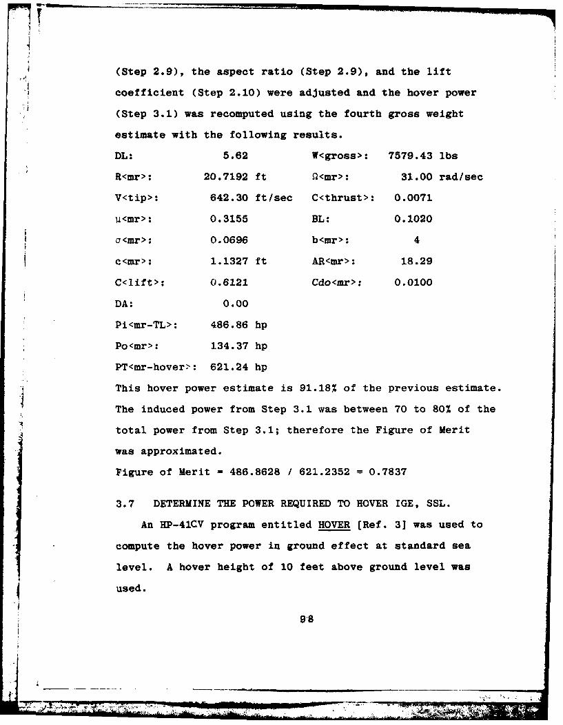
(Step 2.9), the aspect ratio (Step 2.9), and the lift

coefficient (Step 2.10) were adjusted and the hover power

(Step 3.1) was recomputed using the fourth gross weight

estimate with the following results.

DL: 5.62 W<gross>: 7579.43 lbs

R<mr>: 20.7192 ft S<mr>: 31.00 rad/sec


ii<mr>: 0.3155 BL: 0.1020

c<mr>: 0.0696 b<mr>: 4

c<mr>: 1.1327 ft AR<mr>: 18.29

C<lift>: 0.6121 Cdo<mr>: 0.0100

DA: 0.00


Po<mr>: 134.37 hp


This hover power estimate is 91.18% of the previous estimate.

The induced power from Step 3.1 was between 70 to 80% of the

total power from Step 3.1; therefore the Figure of Merit

was approximated.

Figure of Merit = 486.8628 / 621.2352 = 0.7837

3.7 DETERMINE THE POWER REQUIRED TO HOVER IGE, SSL.

An HP-41CV program entitled HOVER [Ref. 3] was used to

compute the hover power in ground effect at standard sea

level. A hover height of 10 feet above ground level was

used.

98

Mpoop-&A

Pi<mr-TL+GE>: 371.7278 hp

Po<mr>: 134.3724 hp

PT<mr-hover-IGE>: 506.1002 hp

3.8 DETERMINE THE PARASITE POWER REQUIRED IN FORWARD

FLIGHT.

Using HD-8 and the latest estimate of gross weight

(7579.43 lbs), the equivalent flat plate area loading is

330.0 psf.

EFPA<FF> = W<gross> / Loading<EFPA>

= 7579.43 / 330.0 - 22.9680 ft2

The values of parasite power have been listed in Table 2.

3.9 DETERMINE MAIN ROTOR POWER REQUIRED AND THE MACH

NUMBER OF THE ADVANCING BLADE TIP FOR FORWARD FLIGHT.

A program entitled FLIGHT [Ref. 3.] for use with the

HP-41CV programmable calculator was used to calculate the

values given in Table 2.

99

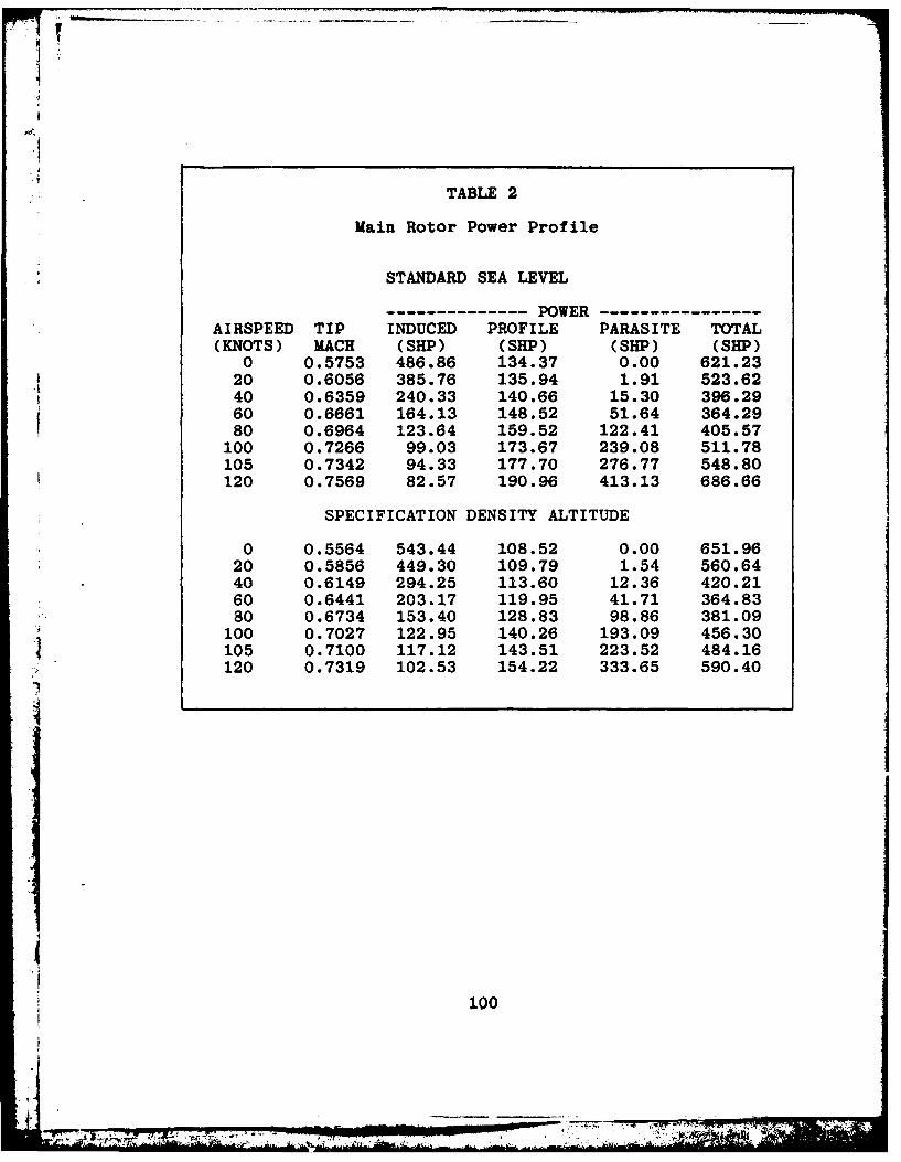
rI

TABLE 2

Main Rotor Power Profile

STANDARD SEA LEVEL

--------------- POWER----------------AIRSPEED TIP INDUCED PROFILE PARASITE TOTAL(KNOTS) MACH (SHP) (SHP) (SHP) (SHP)

0 0.5753 486.86 134.37 0.00 621.2320 0.6056 385.76 135.94 1.91 523.6240 0.6359 240.33 140.66 15.30 396.2960 0.6661 164.13 148.52 51.64 364.2980 0.6964 123.64 159.52 122.41 405.57

100 0.7266 99.03 173.67 239.08 511.78105 0.7342 94.33 177.70 276.77 548.80120 0.7569 82.57 190.96 413.13 686.66

SPECIFICATION DENSITY ALTITUDE

0 0.5564 543.44 108.52 0.00 651.9620 0.5856 449.30 109.79 1.54 560.6440 0.6149 294.25 113.60 12.36 420.2160 0.6441 203.17 119.95 41.71 364.8380 0.6734 153.40 128.83 98.86 381.09

100 0.7027 122.95 140.26 193.09 456.30105 0.7100 117.12 143.51 223.52 484.16120 0.7319 102.53 154.22 333.65 590.40

100

. ... . .. . . .2t l ,

Chapter 4

TAIL ROTOR DESIGN

4.1 MAKE PRELIMINARY DETERMINATIONS OF TAIL ROTOR

GEOMETRY.

HD-9 was used to determine the tail rotor geometry. The

following current main rotor values were required by HD-9.

W<gross>: 7579.43 lbs R<mr>: 20.7192 ft

O<mr>: 31.00 rad/sec (296.0282 RPM) Cdo<mr>: 0.010

The results of the calculations of HD-9 are shown below.

AR<tr>: 6.75 b<mr>: 2 Cdo<tr>: 0.0138

Q<tr>: 139.5 rad/sec (1332.1269 RPM) R<tr>: 3.5790 ft

L<tr> = R<mr> + R<tr> + 0.5 ft

= 20.7192 + 3.5790 + 0.5 = 24.7982 ft

c<tr> = R<tr> / AR<tr>

= 3.5790 / 6.75 = 0.5302 ft

a<tr> - b<tr> * c<tr> / (r * R<tr>)

= 2 * 0.5302 / 3.14 * 3.5790 = 0.0943

4.2 DETERMINE TAIL ROTOR POWER REQUIRED AT HOVER OGE, SSL.

The total power of the tail rotor required to hover

out-of-ground effect at standard sea level was calculated

using the HP-41CV calculator program entitled Hover (Ref.

3]. The tail rotor thrust calculated below should be used

for the value of weight called for in the program.

101

0-

PT<mr>: 621.2346 hp (341,679.03 ft-lbs)

L<tr>: 24.7982 ft O<mr>: 31.00 rad/sec

T<tr> - PT<mr-hover> / ( Q<mr> * L<tr> )

= 341,679.03 / (31.00 * 24.7982) = 444.4639 lbs

The other input values required by the calculator program

are listed below.

AR<tr>: 6.75 R<tr>: 3.5790 ft

b<mr>: 2 Cdo<tr>: 0.0138

<tr>: 139.5 rad/sec c<tr>: 0.5302 ft

The following values were output.

Pi<TL-tr>: 43.1150 hp

Po<tr>: 3.5211 hp

PT<tr-hover>: 46.6360 hp

4.3 DETERMINE TAIL ROTOR POWER REQUIRED AND TIP MACH

EFFECTS FOR FORWARD FLIGHT.

These calculations have been made at both standard sea

level and at specification density altitude. The HP-41CV

programs entitled Flight and TR [Ref. 3] were used to

calculate the values listed in Table 3.

102

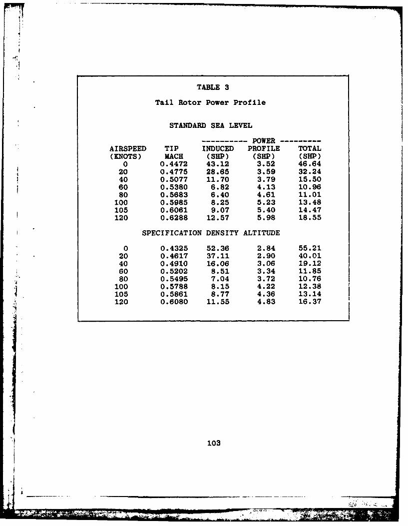
TABLE 3

Tail Rotor Power Profile

STANDARD SEA LEVEL

---------- POWER---------AIRSPEED TIP INDUCED PROFILE TOTAL(KNOTS) MACH ( SHP ) (SHP) (SHP)

0 0.4472 43.12 3.52 46.6420 0.4775 28.65 3.59 32.2440 0.5077 11.70 3.79 15.5060 0.5380 6.82 4.13 10.9680 0.5683 6.40 4.61 11.01

100 0.5985 8.25 5.23 13.48105 0.6061 9.07 5.40 14.47120 0.6288 12.57 5.98 18.55


0 0.4325 52.36 2.84 55.2120 0.4617 37.11 2.90 40.0140 0.4910 16.06 3.06 19.1260 0.5202 8.51 3.34 11.8580 0.5495 7.04 3.72 10.76

100 0.5788 8.15 4.22 12.38105 0.5861 8.77 4.36 13.14120 0.6080 11.55 4.83 16.37

103

.4

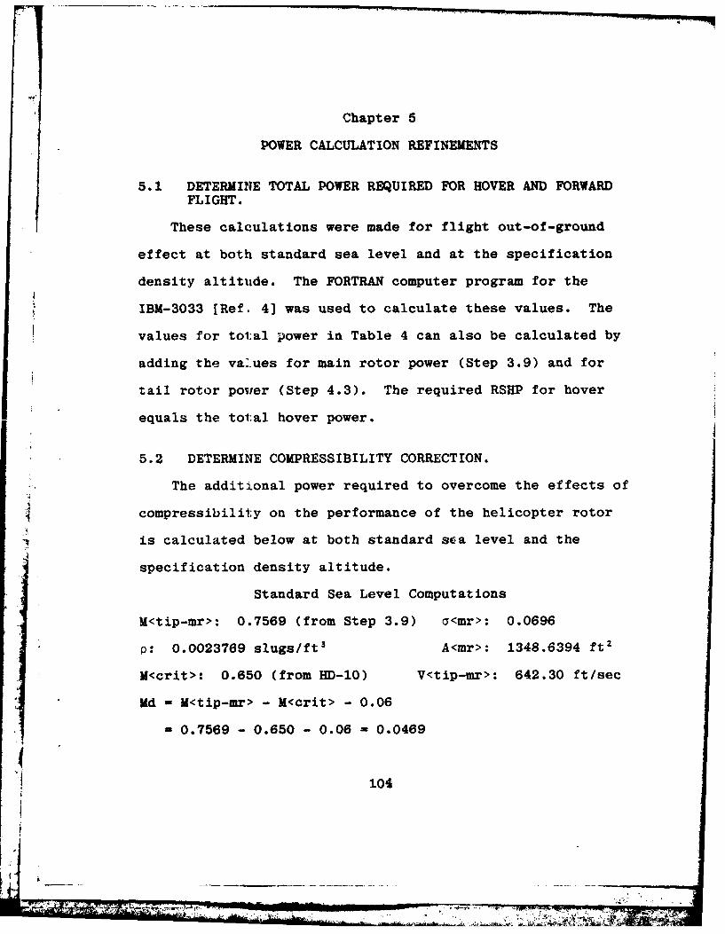
Chapter 5

POWER CALCULATION REFINEMENTS

5.1 DETERMINE TOTAL POWER REQUIRED FOR HOVER AND FORWARD

FLIGHT.

These calculations were made for flight out-of-ground

effect at both standard sea level and at the specification

density altitude. The FORTRAN computer program for the

IBM-3033 [Ref. 4] was used to calculate these values. The

values for total power in Table 4 can also be calculated by

adding the values for main rotor power (Step 3.9) and for

tail rotor power (Step 4.3). The required RSHP for hover

equals the total hover power.

5.2 DETERMINE COMPRESSIBILITY CORRECTION.

The additional power required to overcome the effects of

compressibility on the performance of the helicopter rotor

is calculated below at both standard sca level and the

specification density altitude.

Standard Sea Level Computations

M<tip-mr>: 0.7569 (from Step 3.9) a<mr>: 0.0696

p: 0.0023769 slugs/ft 3 A<mr>: 1348.6394 ft2

M<crit>: 0.650 (from HD-IO) V<tip-mr>: 642.30 ft/sec

Md - M<tip-mr> - M<crit> - 0.06

- 0.7569 - 0.650 - 0.06 = 0.0469

t*( 104

J1117 F 7 ,"7

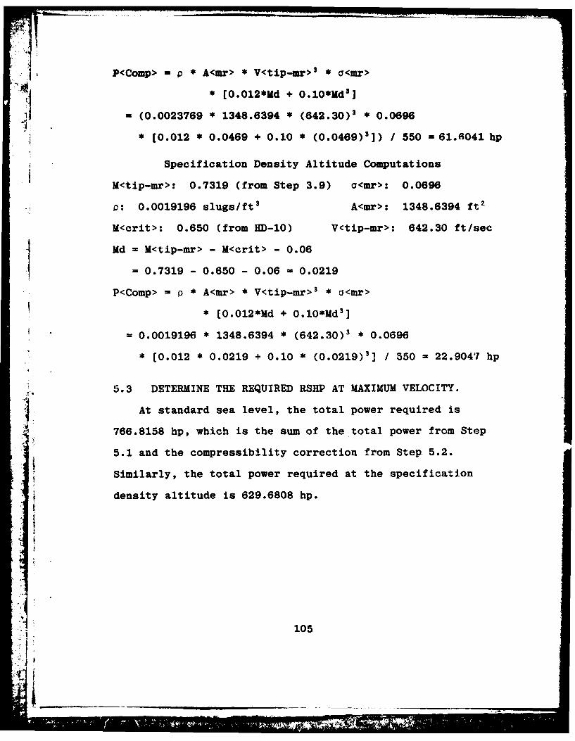
P<Comp> -p *A<mr> *V<tip-mr> * a<mr>

* [0.012*Md + O.10*MdJ

-(0.0023769 * 1348.6394 * (642.30) * 0.0696

*[0.012 * 0. 0469 + 0. 10 * (0. 0469) 3]) / 550 -61.6041 hp

Specification Density Altitude Computations

M<tip-mr>: 0.7319 (from Step 3.9) a<mr>: 0.0696

p: 0.0019196 slugs/ft 3 A<mr>: 1348.6394 ft2

M<crit>: 0.650 (from ED-10) V.<tip-mr>: 642.30 ft/sec

Md - M<tiP-mr> - M<crit> - 0.06*1= 0.7319 -0.650 -0.06 = 0.0219

P<Comp> - P* A<mr> *Vc~tip-mr >3 * a<mr>

* (0.012*Md + o.1O*Md 3]

0.0019196 * 1348.6394 * (642.30)3 * 0.0696

*(0.012 * 0.0219 + 0.10 * (0.0219 )3] / 550 =22.9047 hp

5.3 DETERMINE THE REQUIRED RSHP AT MAXIMUM VELOCITY.

At standard sea level, the total power required is

V 766.8158 hp, which is the sum of the total power from Step

5.1 and the compressibility correction from Step 5.2.

Similarly, the total power required at the specification

density altitude is 629.6808 hp.

ii 105

TABLE 4

Total Rotor Power Profile

STANDARD SEA LEVEL

-------------- POWER----------------AIRSPEED INDUCED PROFILE PARASITE TOTAL(KNOTS) (SHP) (SHP) (SHP) (SHP)

0 529.98 137.89 0.00 667.8720 414.41 139.53 1.91 555.8540 252.03 144.45 15.30 411.7960 170.95 152.65 51.64 375.2480 130.04 164.14 122.41 416.59

100 107.28 178.90 239.08 525.26105 103.40 183.10 276.77 563.26120 95.14 196.94 413.13 705.21


0 595.80 111.36 0.00 707.1720 486.41 112.69 1.54 600.64.40 310.31 116.66 12.36 439.3360 211.68 123.29 41.7, 376.6780 160.44 132.56 98.86 391.86

100 131.11 144.48 193.09 468.67105 125.90 147.87 223.52 497.29120 114.08 159.05 333.65 606.78

5.4 DETERMINE THE REQUIRED RSHP FOR HOVER (IGE) AT THESPECIFIED CEILING.

The HP-41CV programs entitled HOVER and TR [Ref. 3] were

used to compute these values. The values of the input

parameters are listed below.

R<mr>: 20.7192 ft O<mr>: 31.00 rad/sec

b<mr>: 4 c<mr>: 1.1327 ft

W<gross>: 7579.4305 lbs Cdo<mr>: 0.0100

DA: 11000.00 ft Hover height: 10 ft

106

ew

Al:-,.,.'>"

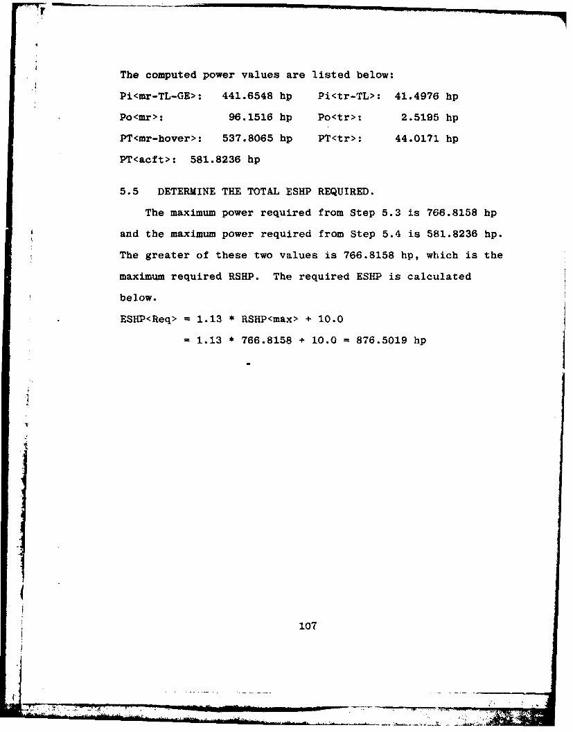
The computed power values are listed below:

Pi<mr-TL-GE>: 441.6548 hp Pi<tr-TL>: 41.4976 hp

Po<mr>: 96.1516 hp Po<tr>: 2.5195 hp

PT<mr-hover>: 537.8065 hp PT<tr>: 44.0171 hp

PT<acft>: 581.8236 hp

5.5 DETERMINE THE TOTAL ESHP REQUIRED.

The maximum power required from Step 5.3 is 766.8158 hp

and the maximum power required from Step 5.4 is 581.8236 hp.

The greater of these two values is 766.8158 hp, which is the

maximum required RSHP. The required ESHP is calculated

below.

ESHP<Req> = 1.13 * RSHP<max> + 10.0

= 1.13 * 766.8158 + 10.0 = 876.5019 hp

107

-7 7

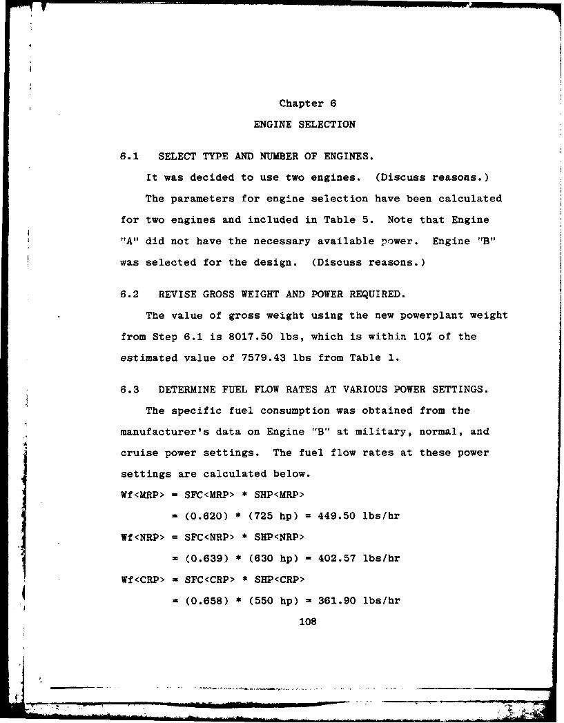
II

Chapter 6

ENGINE SELECTION

6.1 SELECT TYPE AND NUMBER OF ENGINES.

It was decided to use two engines. (Discuss reasons.)

The parameters for engine selection have been calculated

for two engines and included in Table 5. Note that Engine

"A" did not have the necessary available power. Engine "B"

was selected for the design. (Discuss reasons.)

6.2 REVISE GROSS WEIGHT AND POWER REQUIRED.

The value of gross weight using the new powerplant weight

from Step 6.1 is 8017.50 ibs, which is within 10% of the

estimated value of 7579.43 lbs from Table 1.

6.3 DETERMINE FUEL FLOW RATES AT VARIOUS POWER SETTINGS.

The specific fuel consumption was obtained from the

manufacturer's data on Engine "B" at military, normal, and

cruise power settings. The fuel flow rates at these power

settings are calculated below.

Wf<MRP> = SFC<MRP> * SHP<MRP>

= (0.620) * (725 hp) = 449.50 lbs/hr

Wf<NRP> = SFC<NRP> * SHP<NRP>

= (0.639) * (630 hp) - 402.57 lbs/hr

Wf<CRP> = SFC<CRP> * SHP<CRP>

= (0.658) * (550 hp) = 361.90 lbs/hr

108

-.. ... .. . ' ... . ... . .... -.. .. . ..... .. .. . ... . ._

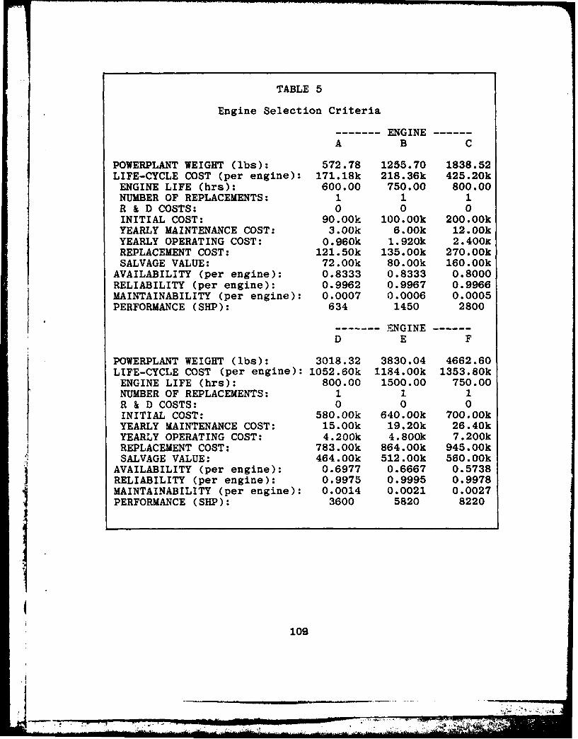
TABLE 5

Engine Selection Criteria

-------- ENGINE------A B C

POWERPLANT WEIGHT (lbs): 572.78 1255.70 1838.52LIFE-CYCLE COST (per engine): 171.18k 218.36k 425.20kENGINE LIFE (hrs): 600.00 750.00 800.00NUMBER OF REPLACEMENTS: 1 1 1R & D COSTS: 0 0 0INITIAL COST: 90.00k 100.00k 200.00kYEARLY MAINTENANCE COST: 3.00k 6.00k 12.00kYEARLY OPERATING COST: 0.960k 1.920k 2.400KREPLACEMENT COST: 121.50k 135.00k 270.00kSALVAGE VALUE: 72.00k 80.00k 160.00k

AVAILABILITY (per engine): 0.8333 0.8333 0.8000RELIABILITY (per engine): 0.9962 0.9967 0.9966MAINTAINABILITY (per engine): 0.0007 0.0006 0.0005PERFORMANCE (SHP): 634 1450 2800

--------- ENGINE------D E F

POWERPLANT WEIGHT (lbs): 3018.32 3830.04 4662.60LIFE-CYCLE COST (per engine): 1052.60k 1184.00k 1353.80kENGINE LIFE (hrs): 800.00 1500.00 750.00NUMBER OF REPLACEMENTS: 1 1 1R & D COSTS: 0 0 0INITIAL COST: 580.00k 640.00k 700.00kYEARLY MAINTENANCE COST: 15.00k 19.20k 26.40kYEARLY OPERATING COST: 4.200k 4.800k 7.200kREPLACEMENT COST: 783.00k 864.00k 945.00kSALVAGE VALUE: 464.00k 512.00k 560.00k

AVAILABILITY (per engine): 0.6977 0.6667 0.5738RELIABILITY (per engine): 0.9975 0.9995 0.9978MAINTAINABILITY (per engine): 0.0014 0.0021 0.0027PERFORMANCE (SHP): 3600 5820 8220

109

-, - .. .. , -2'S.T . v ,

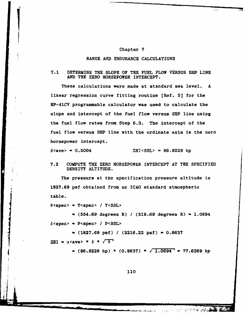
Chapter 7

RANGE AND ENDURANCE CALCULATIONS

7.1 DETERMINE THE SLOPE OF THE FUEL FLOW VERSUS SHP LINE

AND THE ZERO HORSEPOWER INTERCEPT.

These calculations were made at standard sea level. A

linear regression curve fitting routine (Ref. 5] for the

HP-41CV programmable calculator was used to calculate the

slope and intercept of the fuel flow versus SHP line using

the fuel flow rates from Step 6.3. The intercept of the

fuel flow versus SHP line with the ordinate axis is the zero

horsepower intercept.

B<ave> - 0.5004 ZHI<SSL> = 86.9229 hp

7.2 COMPUTE THE ZERO HORSEPOWER INTERCEPT AT THE SPECIFIED

DENSITY ALTITUDE.

The pressure at the specification pressure altitude is

1827.69 psf obtained from an ICAO standard atmospheric

table.

e<spec> - T<spec> / T<SSL>

- (554.69 degrees R) / (518.69 degrees R) - 1.0694

6<spec> - P<spec> P<SSL>

- (1827.69 psf) / (2216.22 psf) - 0.8637

ZHI = <ave>*5*

- (86.9229 hp) * (0.8637) * .7 1.0694 = 77.6369 hp

110

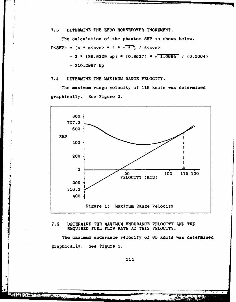
7.3 DETERMINE THE ZERO HORSEPOWER INCREMENT.

The calculation of the phantom SHP is shown below.

P<SHP> - [n * c<ave> * 6 * /"'" / 6<ave>

- 2 * (86.9229 hp) * (0.8637) * /]10694' / (0.5004)

= 310.2987 hp

7.4 DETERMINE THE MAXIMUM RANGE VELOCITY.

The maximum range velocity of 115 knots was determined

graphically. See Figure 2.

800707.2

600

SHP400

200

4 050 100 115 130

VELOCITY (KTS)200

310.3

400

Figure 1: Maximum Range Velocity

7.5 DETERMINE THE MAXIMUM ENDURANCE VELOCITY AND THE

REQUIRED FUEL FLOW RATE AT THIS VELOCITY.

The maximum endurance velocity of 65 knots was determined

'graphically. See Figure 3.See13.

S. ..

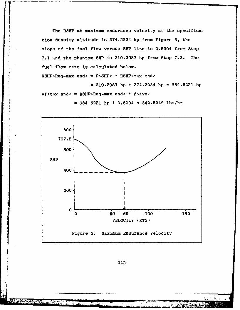
The RSHP at maximum endurance velocity at the specifica-

tion density altitude is 374.2234 hp from Figure 3, the

slope of the fuel flow versus SHP line is 0.5004 from Step

7.1 and the phantom SHP is 310.2987 hp from Step 7.3. The

fuel flow rate is calculated below.

RSHP<Req-max end> = P<SHP> + RSRP<max end>

= 310.2987 hp + 374.2234 hp = 684.5221 hp

Wf<max end> = RSHP<Req-max end> * $<ave>

= 684.5221 hp * 0.5004 = 342.5349 lbs/hr

ir

800

707.2

600.

SHP 400

200

00 5o 65 100 150

VELOCITY (KTS)

Figure 2: Maximum Endurance Velocity

112

-"I,

7.6 DETERMINE THE POWER REQUIRED AT SPECIFICATION CRUISEVELOCITY AND THE REQUIRED FUEL FLOW RATE AT THISVELOCITY.

The RSHP at cruise velocity at the specification density

altitude is 497.2908 hp from Step 5.1, the slope of the fuel

flow versus SHP line is 0.5004 from Step 7.1 and. the phantom

SHP is 310.2987 hp from Step 7.3. The fuel flow rate at

cruise velocity is calculated below.

RSHP<Req-cruise> = P<SHP> + RSHP<cruise>

= 310.2987 hp + 497.2908 hp = 807.5895 hp

Wf<cruise> = RSHP<Req-cruise> * B<ave>

= 807.5895 hp * 0.5004 - 404.1178 lbs/hr

7.7 DETERMINE THE TOTAL FUEL REQUIREMENTS FOR SPECIFIED

MAXI MUM RANGE.

The cruise velocity and maximum range are specification

items from HD-I. The fuel flow rate at normal rated power

for one engine is 402.57 lbs/hr from Step 6.3. The fuel

4 flow rate at maximum endurance velocity is 342.5349 lbs/hr

from Step 7.5. The fuel flow rate at cruise velocity is

404.1178 lbs/hr from Step 7.6. The total fuel requirements

are based on the given assumptions and are calculated below.

FW = 0.05*n*Wf<NRP> + [(Wf<cruise>*RNG<max>) / V<cruise>]

+ 0.05*n*Wf<NRP> + 0.25*Wf<max end>

- (0.05 * 2 * 402.57) + ((404.1178 * 225) / 105]

+ (0.05 * 2 * 402.57) + (0.25 * 342.5349)

. ,- 1032.1144 lbs

113

Chapter 8

MISCELLANEOUS CALCULATIONS

8.1 COMPUTE DESIGN GROSS AND EMPTY WEIGHT.

The estimated fuel weight from Step 3.6 is 1500.0 lbs

and the actual fuel weight from Step 7.7 is 1032.1144 lbs.

The estimated powerplant weight from Step 3.6 is 817.64 lbs

and the actual powerplant weight from Step 6.1 is 1255.70

lbs. The gross weight is therefore 29.8256 lbs lighter than

estimated due to the error in the above estimates. It was

decided to use this shortage for extra fuel. By increasing

the fuel weight, the final design gross weight equals the

weight estimate which was used in the power calculations;

therefore, the power calculations are valid at the final

design gross weight. The additional fuel weight allows for

an increase in the maximum range of the helicopter. The new

maximum range is calculated below.

RNG<max> [V<Cruise> * (FW + FW<Added> - 0.05*n*Wf<NRP>

- 0.05*n*Wf<NRP> - 0.25*Wf<max end>)] / Wf<Cruise>

= [105.0 * (1032.1144 + 29.8256 - (0.05 * 2 * 402.57)

- (0.05 * 2 * 402.57) - (0.25 * 342.5349)] / 404.1178 =

= 232.7494 nmi

8.2 DETERMINE RETREATING BLADE STALL VELOCITY.

The input values for the HP-41CV program entitled BS

[Ref. 6] were:

114

b<mr>: 4 EFPA<FF>: 22.9680 ft 2

.'W<gross>: 7579.4305 lbs c<mr>: 1.1327 ft

R<mr>: 20.7192 ft a<mr>: 31.0 rad/sec

Twist: -10 degrees (Assumption)

CLa: 6.4458 per radian (from Step 2.12)

At a forward velocity of 120 knots the output of the program

is:

Collective: 17.5759 degrees

Cyclic: -6.1871 degrees

Maximum Angle of Attack: 11.7086 degrees

Since the retreating blade does not stall prior to 120

knots, the retreating blade stall velocity is greater than

the specification maximum velocity.

8.3 DETERMINE BEST RATE OF CLIMB.

The minimum total power on the total main rotor power

curve (SSL) is 374.9958 hp at 58 knots. The total rotor

power available at 58 knots is calculated below.

PT<Avail> = (ESHP<Avail> - 10.0) / (0.10*(n-1) + 1.03)

- (1450.0 - 10.0) / 1.13 = 1274.34

The equivalent flat plate area in vertical flight is

calculated below.

EFPA<VF> = 2 * EFPA<FF> - 2 * 22.9680 = 45.9359 ft 2

The HP-41CV programs FLIGHT and TR [Ref. 3] were used to

compute the total main rotor power and the total tail rotor

4115.I

,.* (i

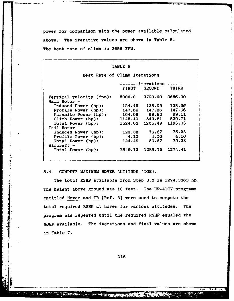
power for comparison with the power available calculated

above. The iterative values are shown in Table 6.

The best rate of climb is 3656 FPM.

TABLE 6

Best Rate of Climb Iterations

------- Iterations-------FIRST SECOND THIRD

Vertical velocity (fpm): 5000.0 3700.00 3656.00Main Rotor -

Induced Power (hp): 124.49 138.09 138.56Profile Power (hp): 147.66 147.66 147.66Parasite Power (hp): 104.09 69.93 69.11Climb Power (hp): 1148.40 849.81 839.71Total Power (hp): 1524.63 1205.49 1195.03

Tail Rotor -

Induced Power (hp): 120.38 76.57 75.28Profile Power (hp): 4.10 4.10 4.10Total Power (hp): 124.49 80.67 79.38

Aircraft -Total Power (hp): 1649.12 1286.15 1274.41

i

8.4 COMPUTE MAXIMUM HOVER ALTITUDE (IGE).

The total RSHP available from Step 8.3 is 1274.3363 hp.

The height above ground was 10 feet. The HP-41CV programs

entitled Hover and TR (Ref. 3] were used to compute the

total required RSHP at hover for various altitudes. The

program was repeated until the required RSHP equaled the

RSHP available. The iterations and final values are shown

in Table 7.

116

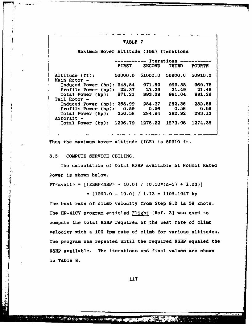
TABLE 7

Maximum Hover Altitude (IGE) Iterations

----------- Iterations-----------FIRST SECOND THIRD FOURTH

Altitude (ft): 50000.0 51000.0 50900.0 50910.0Main Rotor -

Induced Power (hp): 948.84 971.89 969.55 969.78Profile Power (hp): 22.37 21.39 21.49 21.48Total Power (hp): 971.21 993.28 991.04 991.26

Tail Rotor -Induced Power (hp): 255.99 284.37 282.35 282.55Profile Power (hp): 0.59 0.56 0.56 0.56Total Power (hp): 256.58 284.94 282.92 283.12

Aircraft -

Total Power (hp): 1236.79 1278.22 1273.95 1274.38

Thus the maximum hover altitude (IGE) is 50910 ft.

8.5 COMPUTE SERVICE CEILING.

The calculation of total RSHP available at Normal Rated

Power is shown below.

PT<avail> = [(ESHP<NRP> - 10.0) / (0.10*(n-1) + 1.03)]

= (1260.0 - 10.0) / 1.13 - 1106.1947 hp

The best rate of climb velocity from Step 8.2 is 58 knots.

The HP-41CV program entitled Flight (Ref. 3] was used to

compute the total RSHP required at the best rate of climb

velocity with a 100 fpm rate of climb for various altitudes.

The program was repeated until the required RSHP equaled the

RSHP available. The iterations and final values are shown

in Table 8.

117

..........................................

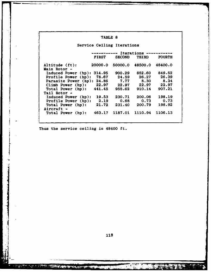
TABLE 8

Service Ceiling Iterations

----------- Iterations--------FIRST SECOND THIRD FOURTH

Altitude (ft): 20000.0 50000.0 48500.0 48400.0Main Rotor -Induced Power (hp): 314.95 900.29 852.60 849.52Profile Power (hp): 78.67 24.59 26.27 26.39Parasite Power (hp): 24.86 7.77 8.30 8.34Climb Power (lp): 22.97 22.97 22.97 22.97Total Power (hp): 441.45 955.62 910.14 907.21

Tail Rotor -Induced Power (hp): 19.53 230.71 200.06 198.19Profile Power (hp): 2.19 0.68 0.73 0.73Total Power (hp): 21.72 231.40 200.79 198.92

Aircraft -Total Power (hp): 463.17 1187.01 1110.94 1106.13

Thus the service ceiling is 48400 ft.

*lie

: Chapter 9

FINAL CHECK

9.1 MAKE FINAL CHECK FOR COMPLIANCE WITH SPECIFICATIONS.

Table 9 is a final summary of this example.

TABLE 9Final Summary

Performance1 Specification DesignCrew:22Internal Load [lbs]: 1000 1000

Max Hover Altitude (IGE): 11000 50910Service Ceiling: 14500 48400Disk Loading: -- 5.62Velocity [kts] - Cruise: 105 105

Maximum: 120 120Max Endurance: -- 65Max Range: -- 115

Retreating Blade Stall: 1750 > 120Best Rate of Climb [fpm]: -- 3656Figure of Merit: -- 0.7837Engine - Number / Type: -- 2 "B"

SHP per engine (Military): -- 725Coefficient of Thrust: -- 0.0071Coefficient of Lift: -- 0.6121Max Advance Ratio: -- 0.3155Maximum Range [nmi]: 225 232.7

GeometryWeight (lbs] - Max Gross: 11000 7579.43

Empty: -- 5117.49Fuel Capacity [lbs] - Internal: -- 1061.94Main Rotor - Airfoil section used: -- "A"

Chord [ft]: -- 1.1327Radius [ft]: < 27 20.7192Number of blades: -- 4Drag Coefficient: -- 0.010

Rotational velocity [rad/sec]: -- 31.0Solidity: -- 0.0696Aspect Ratio: -- 18.29

Tail Rotor - Airfoil section used: -- "A"Chord [ft]: -- 0.5302

119

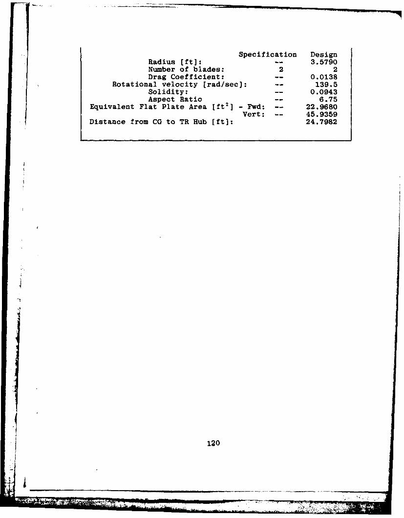
Specification DesignRadius [ft]: -- 3.5790Number of blades: 2 2Drag Coefficient: -- 0.0138

Rotational velocity [rad/sec]: -- 139.5Solidity: -- 0.0943Aspect Ratio [ft2 6.75

Equivalent Flat Plate Area ft]-Fwd: -- 22.9680Vert: -- 45.9359

Distance from CG to TR Hub [ft]: 24.7982

120

.4~ ~ ~ ~ ~ ~ ~ ~ ~~~~~UMVN i ______________________________ ____

LIST OF REFERENCES

1. Kee, S. G., Helicopter Design Manual, Naval Post-graduate School, Monterey, CA, 1983.

2. Abbott, Ira A. and Von Duenhoff, Albert E., Theory ofWing Sections, Dover Publications, 1959.

3. Fardink, Paul J., Hand-Held Computer Programs forPreliminary Helicopter Design, M.S. Thesis, NavalPostgraduate School, Monterey, CA, 1982.

4. Sullivan, Patrick, Helicopter Power Computation Package(FORTRAN), Term Paper for AE4900 (Professor Layton),Naval Postgraduate School, Monterey, CA, 1982.

5. Hewlett-Packard Co., Standard Applications Handbook,pp. 42-48, 1981.

6. Layton, Donald M., BS, Program for HP-41CV ProgrammableCalculator, Naval Postgraduate School, Monterey, CA,1980.

121

w

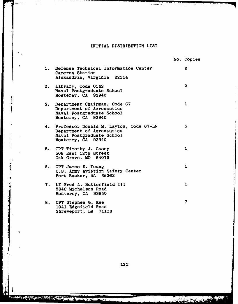
INITIAL DISTRIBUTION LIST

No. Copies

1. Defense Technical Information Center 2Cameron StationAlexandria, Virginia 22314

2. Library, Code 0142 2Naval Postgraduate SchoolMonterey, CA 93940

3. Department Chairman, Code 67 1Department of AeronauticsNaval Postgraduate SchoolMonterey, CA 93940

4. Professor Donald M. Layton, Code 67-LN 5Department of AeronauticsNaval Postgraduate SchoolMonterey, CA 93940

5. CPT Timothy J. Casey 1508 East 12th StreetOak Grove, MO 64075

6. CPT James E. Young 1U.S. Army Aviation Safety CenterFort Rucker, AL 36362

7. LT Fred A. Butterfield III 1584C Michelson RoadMonterey, CA 93940

8. CPT Stephen G. Kee 71041 Edgefield RoadShreveport, LA 71118

122

--.

Documents

NAVAL POSTGRADUATE SCHOOLdtic.mil/dtic/tr/fulltext/u2/a128974.pdf · NAVAL POSTGRADUATE SCHOOL Monterey, California iM-DTIC I1ELECTE i1 THESIS D GUIDE FOR CONCEPTUAL HELICOPTER DESIGN