NAVAL POSTGRADUATE SCHOOL · NAVAL POSTGRADUATE SCHOOL Monterey, California In 0 THESIS DESIGNING AN AUTOMATIC CONTROL SYSTEM ... Master's Thesis From To December 1988 183 16 Supplementary

NAVAL POSTGRADUATE SCHOOLMonterey, California

In

0 THESISDESIGNING AN AUTOMATIC CONTROL SYSTEM

FOR A SUBMARINE

by

Orhan K. Babaoglu

December 19S8

Thesis Advisor George J. Thaler

Approved For public release. distribution is unlinited. DD T ICAftELECTE

SFEB 141

H

89 2 13 187

Unclassifiedsecurity classification of this pace

REI'ORT DOCUMENIAIION PAGEI a Report Security Classification Unclassified Ib Restrictive markings

2a Security Classification Authority 3 Distribution Availability of Report2b Declassification Downgrading Schedule Approved for public release; distribution is unlimiited.4 Performing Organization Report Number(s) 5 Monitoring Organization Report Number(s)6a Name of Performing Organization 6b Office Symbol 7a Name of Mcnitoring OrganizationNaval 1lostiaraduate School Nif,2ppllcable) 33 Naval Postgraduate Sc'iool6c Address (city. state. and ZIP code) 7b Address (cit, state, and ZIP code)Monterey. CA 93943-5000 Monterey. CA 93943-50008a Name of Funding Sponsoring Organization 8b Office Symbol 9 Procurement Instrument Identification Number

(if" applicable)8c Address (cliy, state, and ZIP code) 10 Source of Funding Numbers

Program Element No Project No Trask No Work Unit Accession No

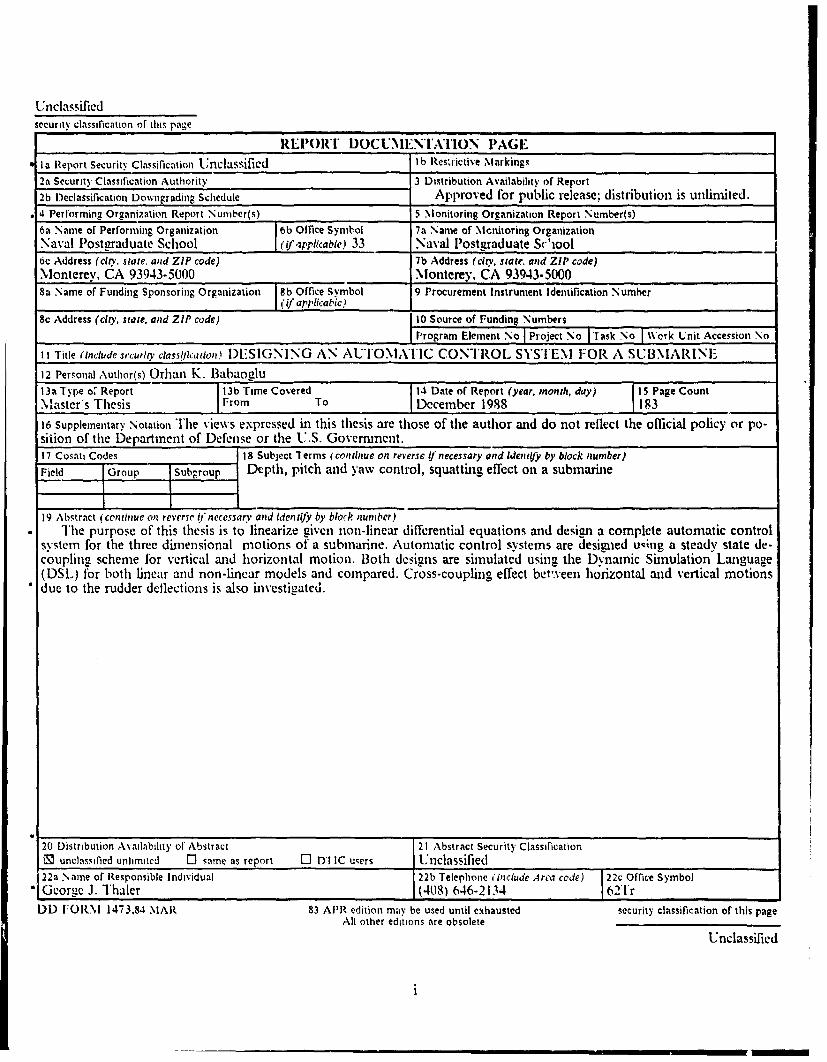
II Title (Include securlty classfi7cation) I)FLSIGNING AN AUTOMATIC CONTROL SYSTEM FOR A SUBMARINE

12 Personal Author(s) Orhzn K. Babaoglu13a Type o, Report 13b T-ime Covered 14 Date of Report (year, month, day) 15 Page CountMaster's Thesis From To December 1988 18316 Supplementary Notation The views expressed in this thesis are those of the author and do not rellect the official policy or po-si0ion of the Department of Defense or the U.S. Government.17 Cosati Codes 18 Subject 1Terms (continue on reverse iJ necessary and ldentiJy by block number)Field Group Subgroup Depth, pitch and yaw control, squatting effect on a submarine

19 Abstract (continue on reverse itI necessanr and ldentify by block number)"The purpose of this thesis is to linearize given non-linear differential equations and design a complete automatic control

system for the three dimensional motions of a submarine. Automatic control systems are desimied uving a steady state de-coupling scheme for vertical and horizontal motion. Both designs are simulated using the Dynamic Simulation Language(DSL) for both linear and non-linear models and compared. Cross-coupling effect bet',veen horizontal and vertical motionsdue to the rudder deflections is also investigated.

20 Distribution Availability of Abstract 21 Abstract Security ClassificationM unclassified unlimited M same as report El DTIC users Unclassified22a Name of Responsible Individual 22b Telephone finclude Area code) 22c Office SymbolGeorge J. Thaler (408) 646-2134 62Tr

DD FORMI 14713,84 MAR 83 APR edition may be used until ex.hausted security classification of this pageAll other editions are obsolete

Unclassified

1 •

Approved 11or public release; distribution is unlinmited.

Designing an Automautic Control System lor a Submarine

by

Orlian K. IhmbaogluLieutenant Junior Cirade,Turkisli Navy

B.S., Turkish Naval Academy, 1982

Subnfitted in partial Fufilil~ment of therequirements lur the degree of'

MAljSTlER 017 SCIE'NCE IN ELECTRICAL ENGINEERING

From the

NIAVAL POSTG RADULATE SCI IQOL

Author:

Approved by:

gal Titus, Second Reader

John P1. Powers. Chairman,Department of Electrical and Computer Engineering

Gordon E. Schacher,Dean or Science and En'incering

ABSTRACT

The purpose of this thesis is to linearize given non-linear difflrential equations and

design a complete automatic control system for the three dimensional motions of a

submarine. Automatic control systcms are designed using a steady state decoupling

scheme for vertical and horizontal motion. Both designs are simulated using the Dy.

nanic Simulation Language (DSL) for both linear and non-linear models and compared.

Cross-coupling effect between horizontal and vertical motions due to the rudder de-

flections is also investigated. (:/u--- -

Acoession Fo r

NTIS GRA&IDTIC TAB 1-

Unarmouneaad "Just ificat io-

ByDistribution/

Availability Codes

tAvail and/orIDist SpOcialj ' _ _ _

Ilio.

TABLE OF CONTENTS

1. IN TRODUCTION ............................................. 1

11 EQUATIONS OF MOTiONS IN SIX DEGREES OF FREEDOM ........ 3

A. BACKGROUND ........................................... 3

B. DERIVATION OF THE LINEARIZED MODEL ................... 5

1. A ssum ptions ............................................. 5

2. Derivation of the linear equations of Motion .................... 6a. Linearization on the vertical plane ......................... 6

b. Linearization on the Ilorizontal Plane ...................... 7

C. VALIDATION OF LINEAR MODEL .......................... I I1. Validation of Linear Model on Vertical Plane ................... 11

a. Initial Condition Response .............................. 11

b. Forced Response ..................................... 12

2. Validation of the Linear Model oa the Horizontal Plane ........... 41a. Initial Condition Response .............................. 42

b. Forced Response ..................................... 48

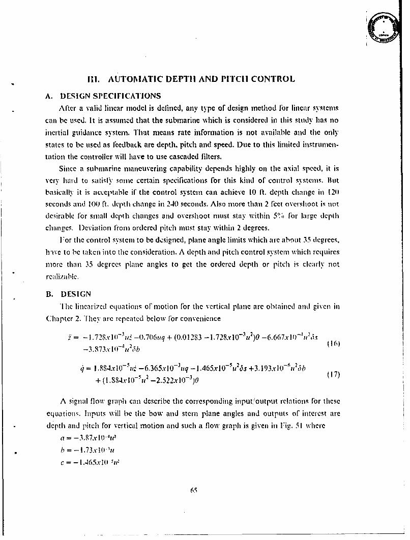
111. AUTOMATIC DEPTH AND PITCH CONTROL ................... 65

A. DESIGN SPECIFICATIONS .................................. 65

B. D ESIG N ...................................... .......... 65

I. D ecoupling ............................................. 66

2. D esign ................................................ 68

a. Lim iters ........................................... 79

b. A ctuators .......................................... 82

3. Sim ulation ............................................. 83

IV. AUTOMATIC STEERING CONTROL ........................... 97

A. DESIGN SPECIFICATIONS .................................. 97

B. D ESIGN. ................................................. 98

1. D ecoupling ............................................. 99

2. Sim ulation ............................................ 103

iv

V. VALIDATION OF TilE COMPENSATED NON-LINEAR MODEL ..... 117

A . SIM IJLATION ....................... ................... 117

VI. CONCLUSIONS AND RECOMMENDATIONS FOR FURTHER WORK 136

A. CONCLUSIONS ............. ............................. 136

B. RECOMMENDATIONS FOR IFURTHER WORK ................ 136

APPENDIX A. DEFINITIONS OF SYMBOLS ....................... 138

APPENDIX B. HYDRODYNAMIC COEFFICIENTS OF SIMULATION

EQ UA TIO N S .................................................. 142

A. AXIAL FORCE ........................................... 142

B. LATERAL FORCE ........................................ 142

C. NORMAL FORCE ........................................ 142

D. ROLLING MOMENT ...................................... 143

E. PITCHING MOMENT ..................................... 143

F. YAW ING MOMENT . ...................................... 143

G . O TIIERS ................................................ 143

APPENDIX C. STANDARD EQUATIONS OF MOTION ............... 144

A . AXIAL FORCE ........................................... 144B. LATERA•L FORCE ......................................... 145C. NORL T AL FORCE ........................................ 146

D. ROLLING M OM ENT ...................................... 147

E. PITCHING MOMENT ..................................... 148

F. YAW ING MOM ENT ...................................... 149

G. AUXILARY EQUATIONS .................................. 150

APPENDIX D. SIMULATION PROGRAM FOR LINEARIZED VERTICAL

EQUATIONS OF MOTION . ...................................... 151

APPENDIX E. SIMULATION PROGIRAM FOR LINEARIZED IIORIZON-

TAL EQUATIONS OF MOrION .................................. 152

v

APPENDIX F. SIMULATION PROGRAM FOR THE COMPENSATED SYS-TEM IN VERTICAL MOTION .................................... 154

APPENDIX G. SIMULATION PROGIRAM FOR THE COMPENSATEDSYSTEM IN HORIZONTAL MOTION ............................. 156

APPENDIX H. SIMULATION PROGRAM FOR NON-LINEAR

EQUATIONS OF MOTION ...................................... 158

APPENDIX I. COMPENSATED NON-LINEAR MODEL ............... 162

LIST OF REFERENCES .......................................... 167

INITIAL DISTRIBUTION LIST ................................... 169

vi

LIST OF FIGURES

Figure 1. A Submarine with Axes of Motion ............................ 4Figure 2. Block Diagram for the Linearized Model on the Vertical Plane ........ 8

Figure 3. Block Diagram flor the Linearized Model on the Horizontal Plane .... 10

Figure 4. Initial Condition Response hit. Pitch-5 Deg. U-5 Kts ........... 13

Figure 5. Initial Condition Response Init. Pitch- 5 Deg. U - 8 Kts ........... 14

Figure 6. Initial Condition Response Init. Pitch -5 Deg. U 12 Kts .......... 15

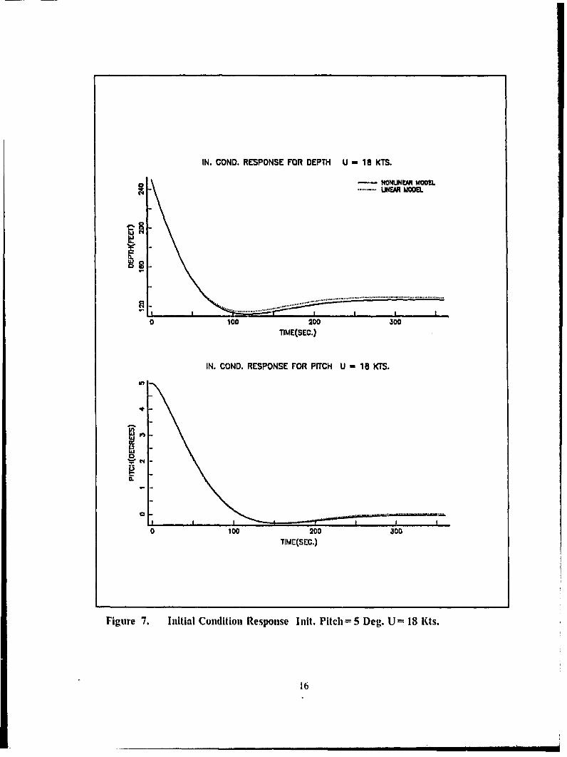
Figure 7. Initial Condition Response Init. Pitch= 5 Deg. U 18 Kts .......... 16

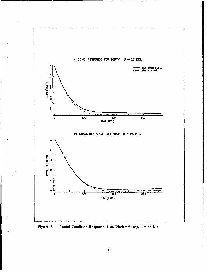
Figure 8. Initial Condition Response Init. Pitch= 5 Deg. U -25 Kts .......... 17

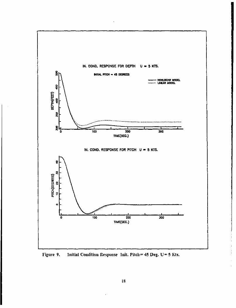
Figure 9. Initial Condition Response Init. Pitch- =45 Deg. U = 5 Kts .......... 18

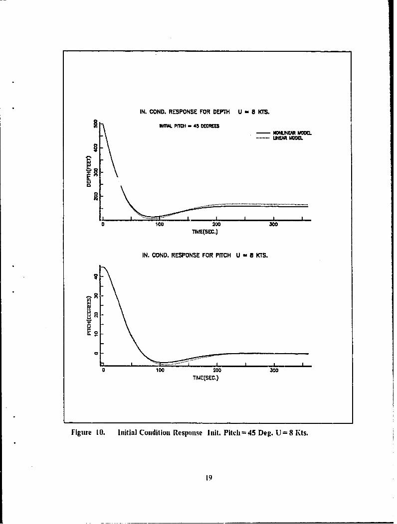
Figure 10. Initial Condition Response Init. Pitchl= 45 Deg. U-- 8 Kts .......... 19

Figure i1. Initial Condition Response Init. Pitch-= 45 Deg. U 12 Kts ......... 20

Figure 12. Forced Response. Bow Plane = 5 Deg. down. U = 5 Kts .......... 22

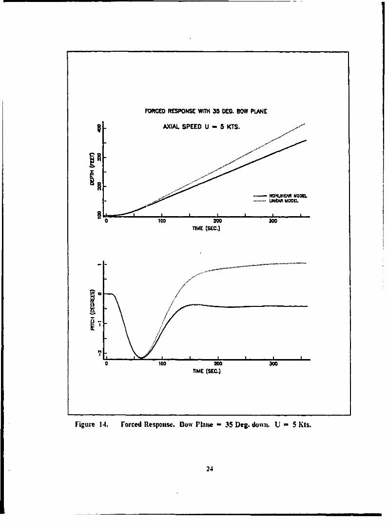
Figure 13. Forced Response. Bow Plane = 15 Deg. down. U = 5 Kts ......... 23Figure 14. Forced Response. Bow Plane = 35 Deg. down. U = 5 Kts . ....... 24

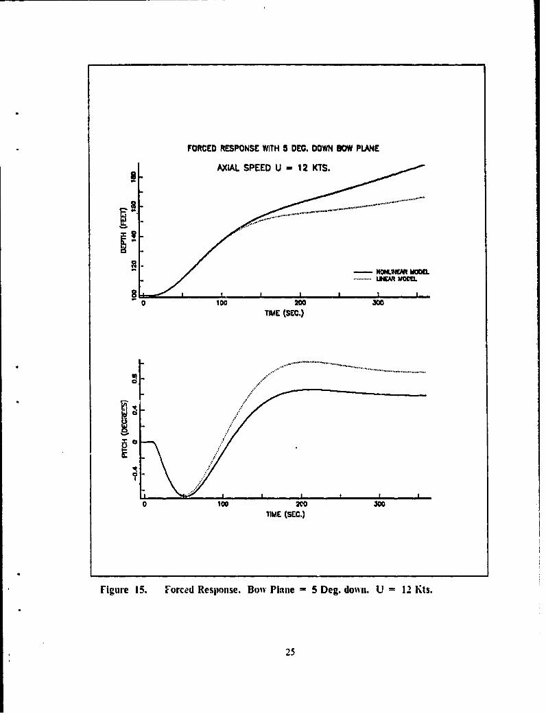
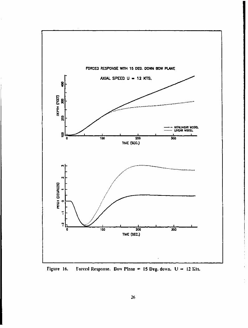
Figure 15. Forced Response. Bow Plane = 5 Deg. down. U - 12 Kts ......... 25Figure 16. Forced Response. Bow Plane = 15 Deg. down. U - 12 Kts ........ 26

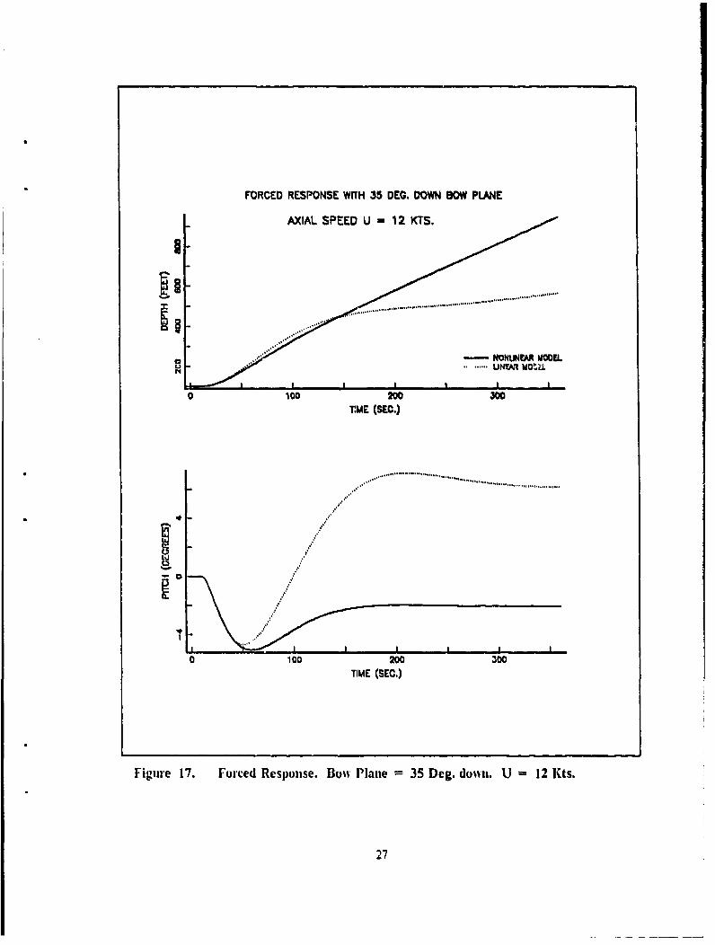
Figure 17. Forced Response. Bow Plane = 35 Deg. down. U = 12 Kts ........ 27

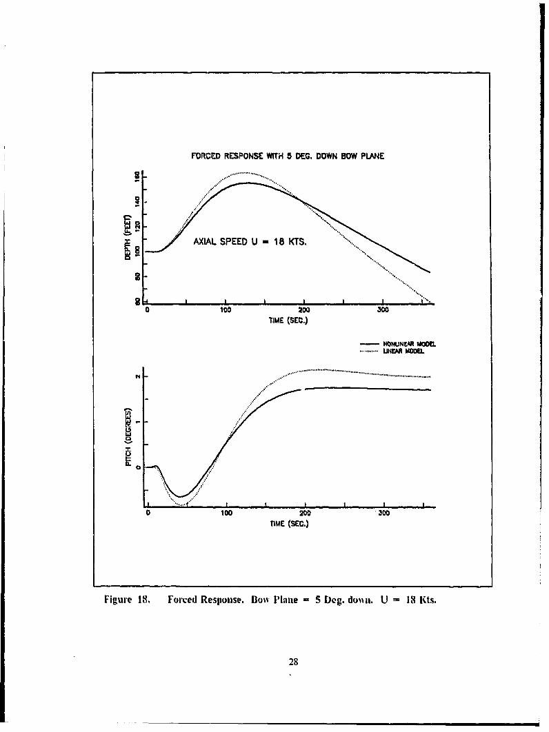
Figure 18. Forced Response. Bow Plane = 5 Deg. down. U - IS Kts ........ 28

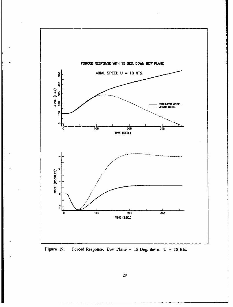
Figure 19. Forced Response. Bow Plane = 15 Deg. down. U = 18 Kts ........ 29

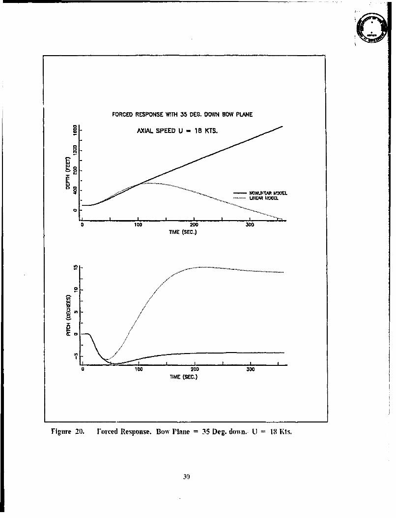
Figure 20. Forced Response. Bow Plane = 35 Deg. down. U - 18 Kts ........ 30

Figure 21. Forced Kesponse. Stern Plane = 5 Deg. U 5 S Kts .............. 32

Figure 22. Forced Response. Stern Plane = 15 Deg. U - 5 Kts ............. 33

Figure 23. Forced Response. Stern Plane 35 Deg. U 5 Kts ............. 34

Figure 24. Forced Response. Stern Plane 5 Deg. U 12 Kts ............. 35

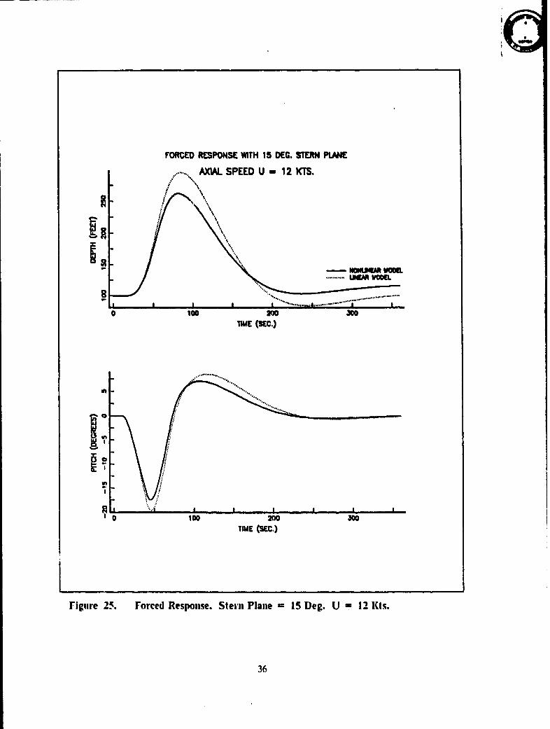
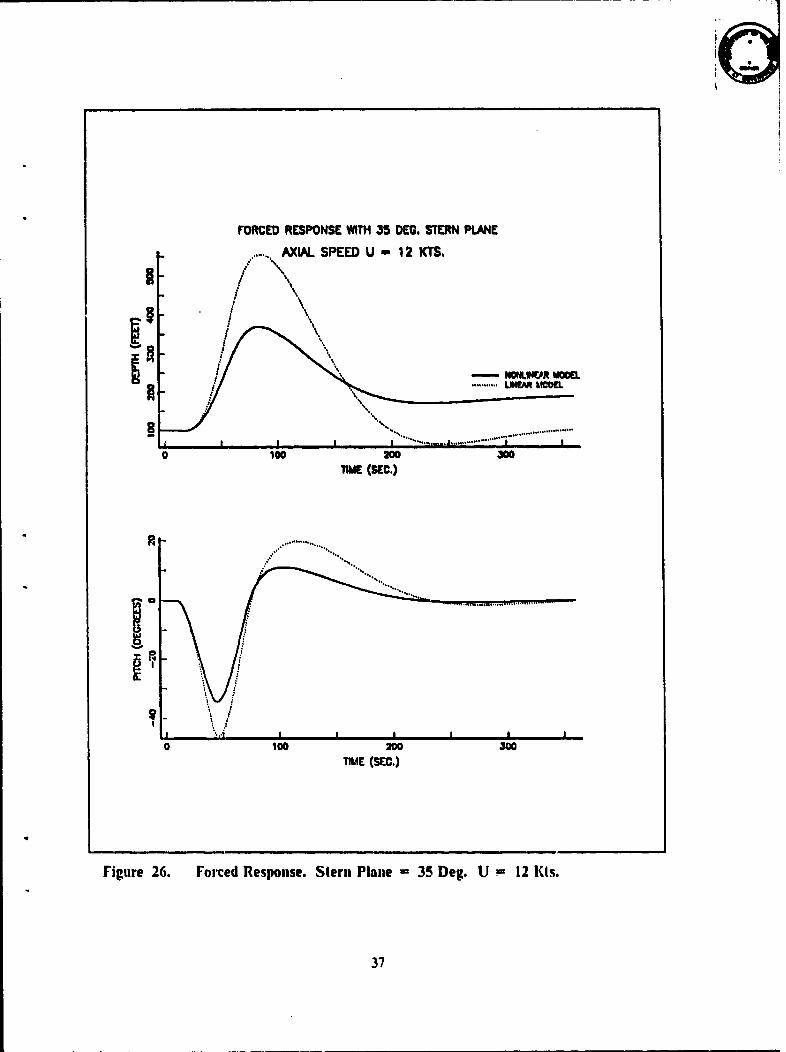
Figure 25. Forced Response. Stern Plane - 15 Deg. U - 12 Kts ............ 36Figure 26. Forced Response. Stern Plane = 35 Deg. U - 12 Kts ............ 37

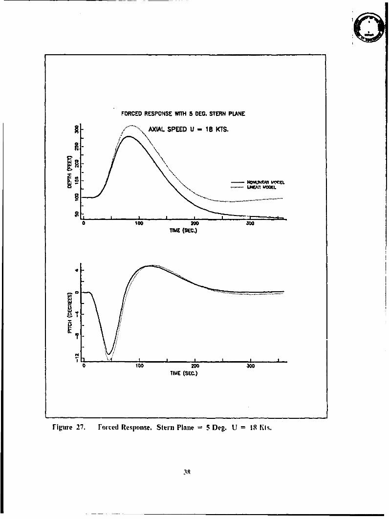
Figure 27. Forced Response. Stern Plane = 5 Deg. U I IS Kts ............. 38

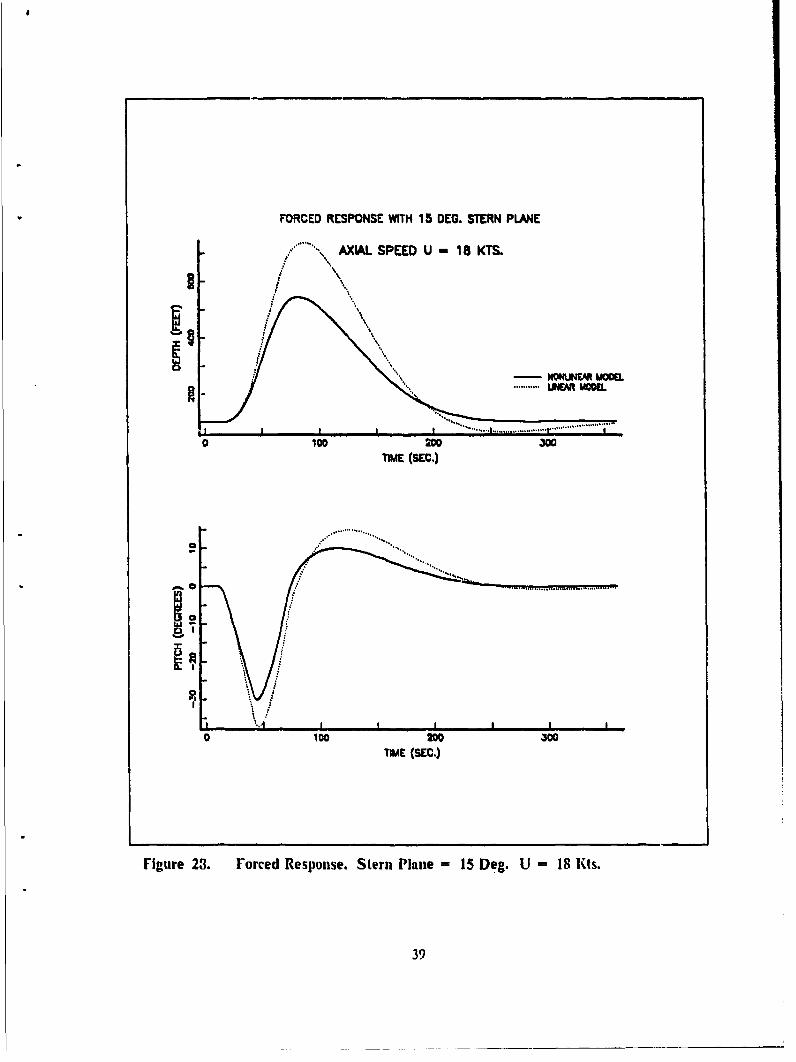
Figure 28. Forced Response. Stern Plane = 15 Deg. U = 18 Kts ............ 39

Figure 29. Forced Response. Stern Plane = 35 Deg. U = 1 Kts ............ 40Figure 30. Initial Condition Response Init. Roll- 5 Deg. U-- 5 and 8 Kts ...... 43

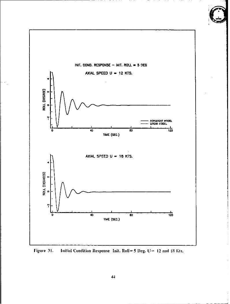
Figure 31. Initial Condition Response Init. Roll= 5 Deg. U = 12 and 18 Kts .... 44

'ii

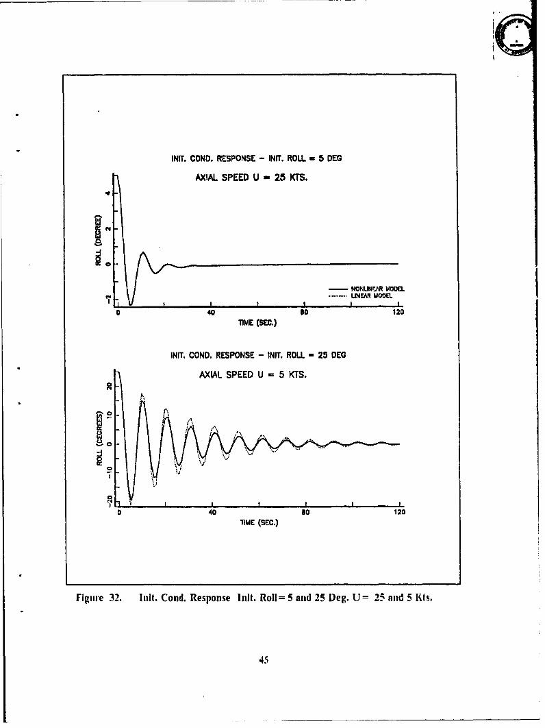
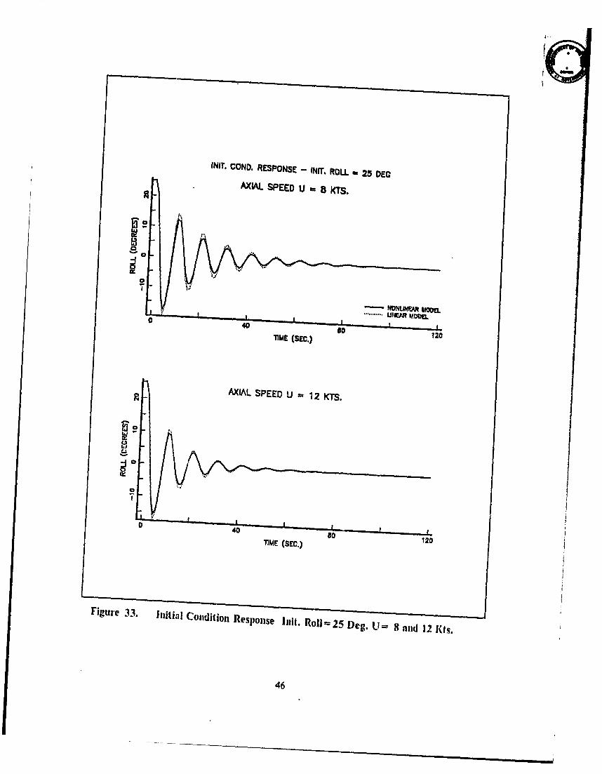
Figure 32. Init. Cond. Response lnit. Roll= 5 and 25 Deg. U = 25 and 5 Kts. .. 45Figure 33. Initial Condition Response lnit. Roll 25 Deg. U- 8 and 12 Kts.... 46

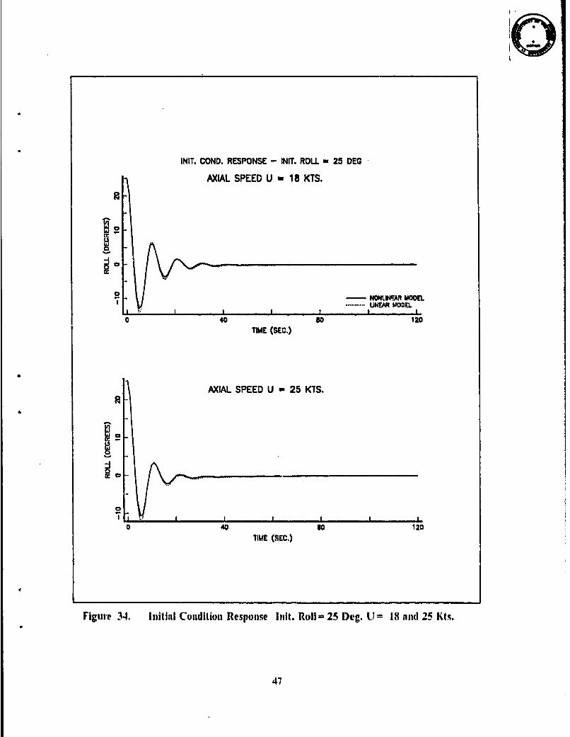
Figure 34. Initial Condition Response I nit. RollI 25 Deg. U 18 and 25 Kts... 47

Figure 35. Forced Response. Rudder = 5 Deg. U = 5 Kts ................. 49

Figure 36. Forced Response. Rudder = 15 Deg. U = 5 Kts . .............. 50

Figure 37. Forced Response. Rudder = 35 Deg. U - 5 Kts . .............. 51

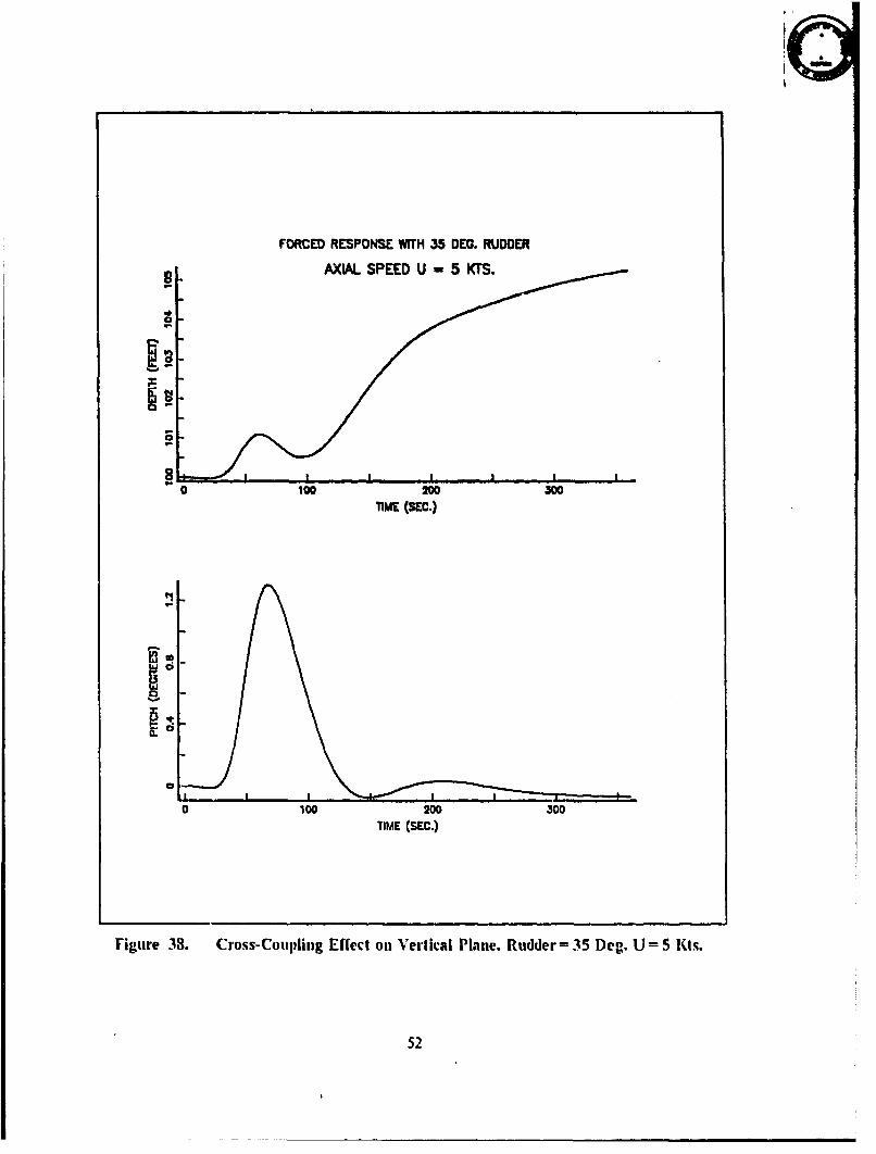
Figure 38. Cross-Coupling LEl'Tbct on Vertical Plane. Rudder= 35 Deg. U-- 5 Kts.. 52

Figure 39. Forced Response. Rudder = 5 Deg. U - 12 Kts ............... 53

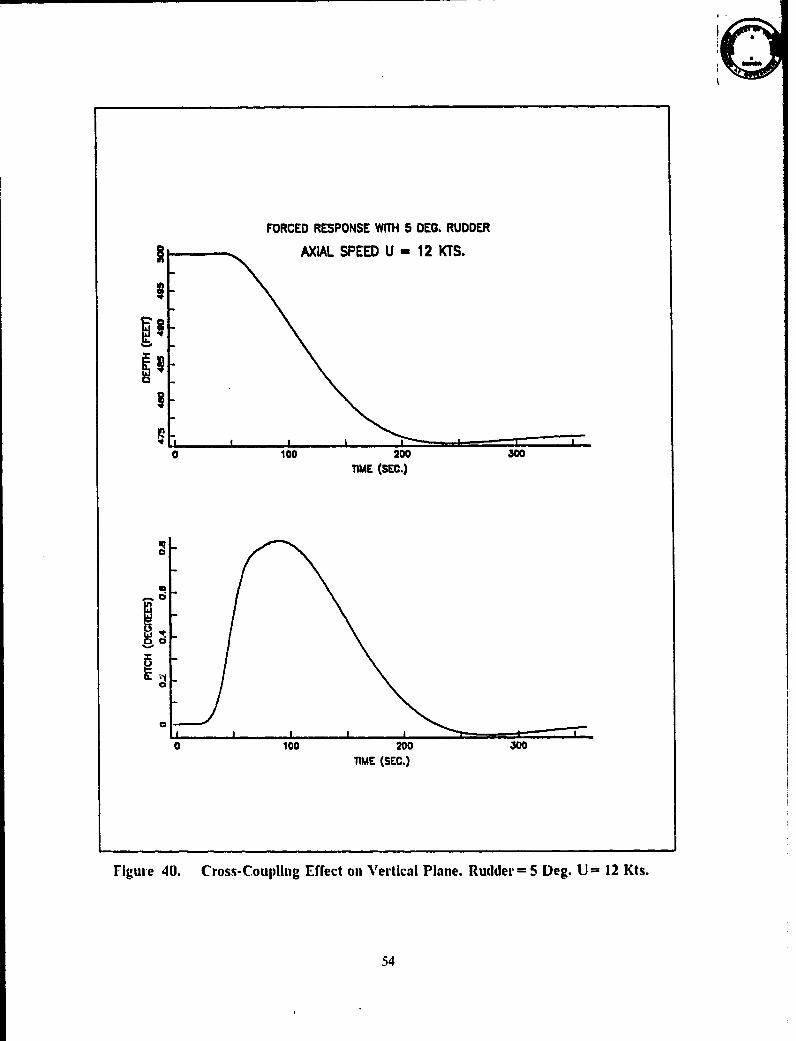
Figure 1. Cross-Coupling [lI lbct on Vertical Plane. Rudder = 5 Deg. U = 12 Kts. . 54

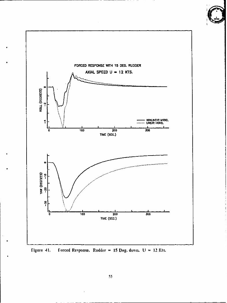
Figure 41. Forced Response. Rudder = 15 Deg. down. U = 12 Kts .......... 55

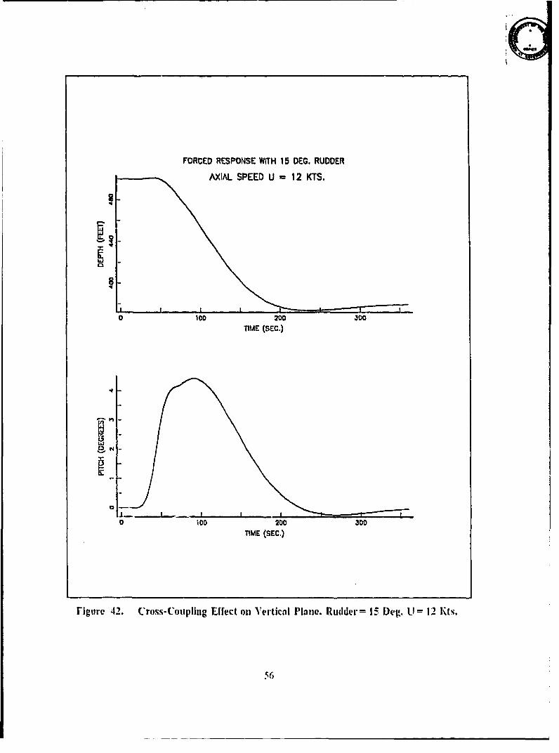
Figure 42. Cross-Coupling Effect on Vertical Plane. Rudder= 15 Deg. U- 12 Kts. 56

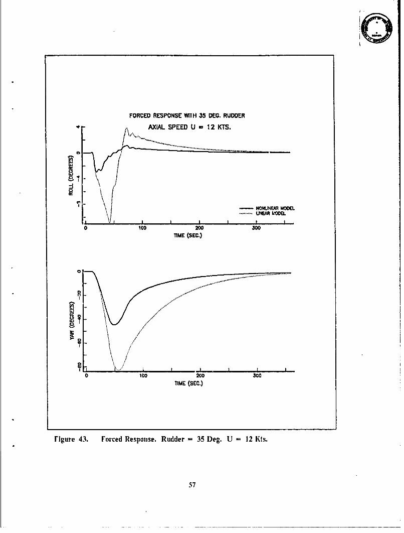
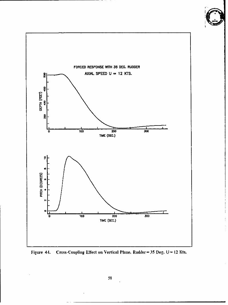
Figure 43. Forced Response. Rudder = 35 Deg. U = 12 Kts ............... 57Figure 44. Cross-Coupling Effect on Vertical Plane. Rudder-= 35 Deg. U = 12 Kts. 58

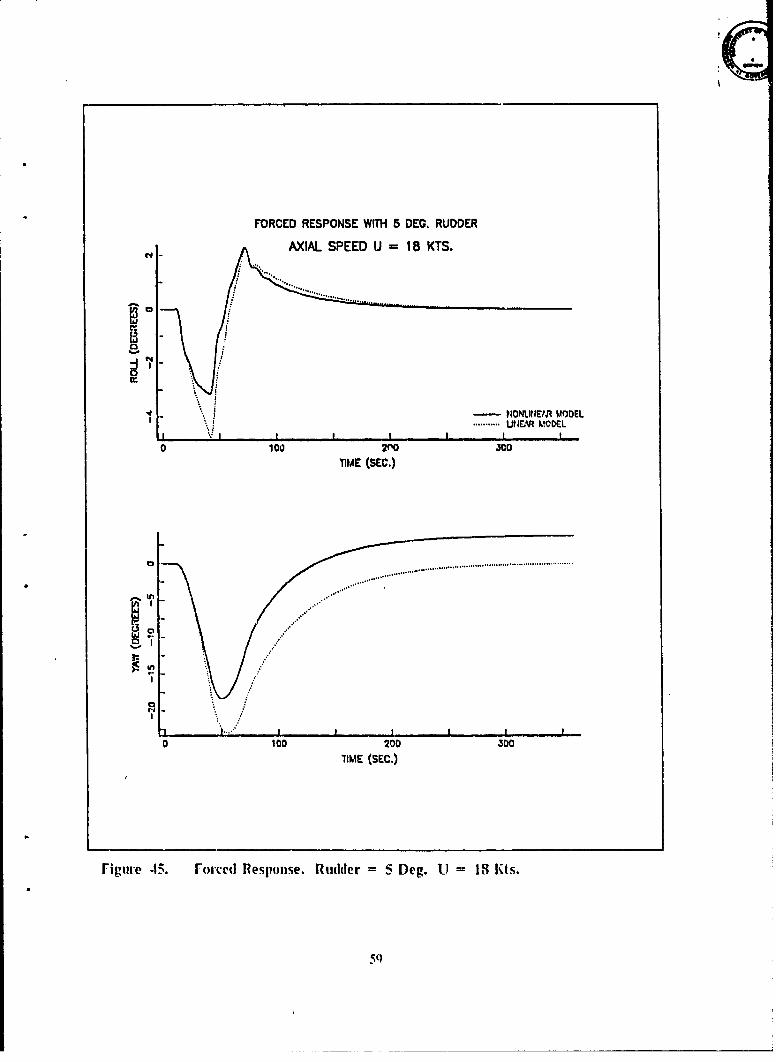
Figure 45. Forced Response. Rudder = 5 Deg. U = 18 Kts . .............. 59

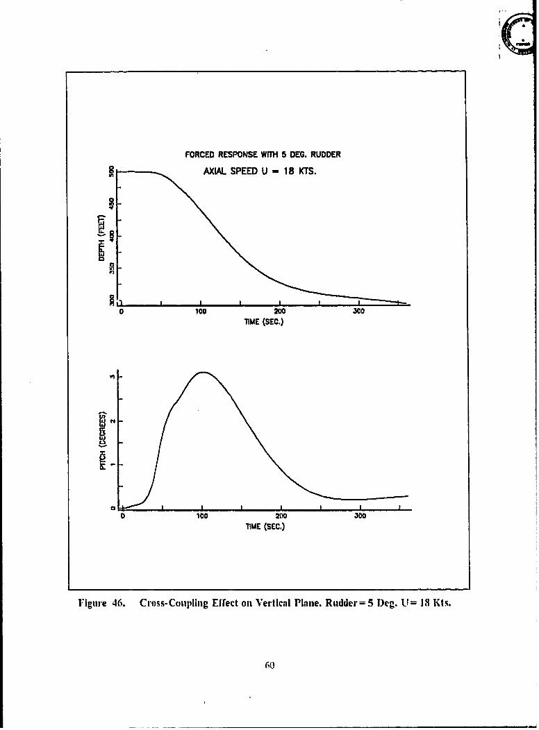
Figure 46. Cross-Coupling Effect oni Vertical Plane. Rudder= 5 Deg. U = 18 Kts. . 60

Figure 47. Forced Response. Rudder = 15 Deg. U = 18 Kts .............. 61

Figure 48. Cross-Coupling Effect on Vertical Plane. Rudder- 15 Deg. U= 18 Kts. 62

Figure 49. Forced Response. Rudder = 35 Deg. U = 18 Kts ............... 63

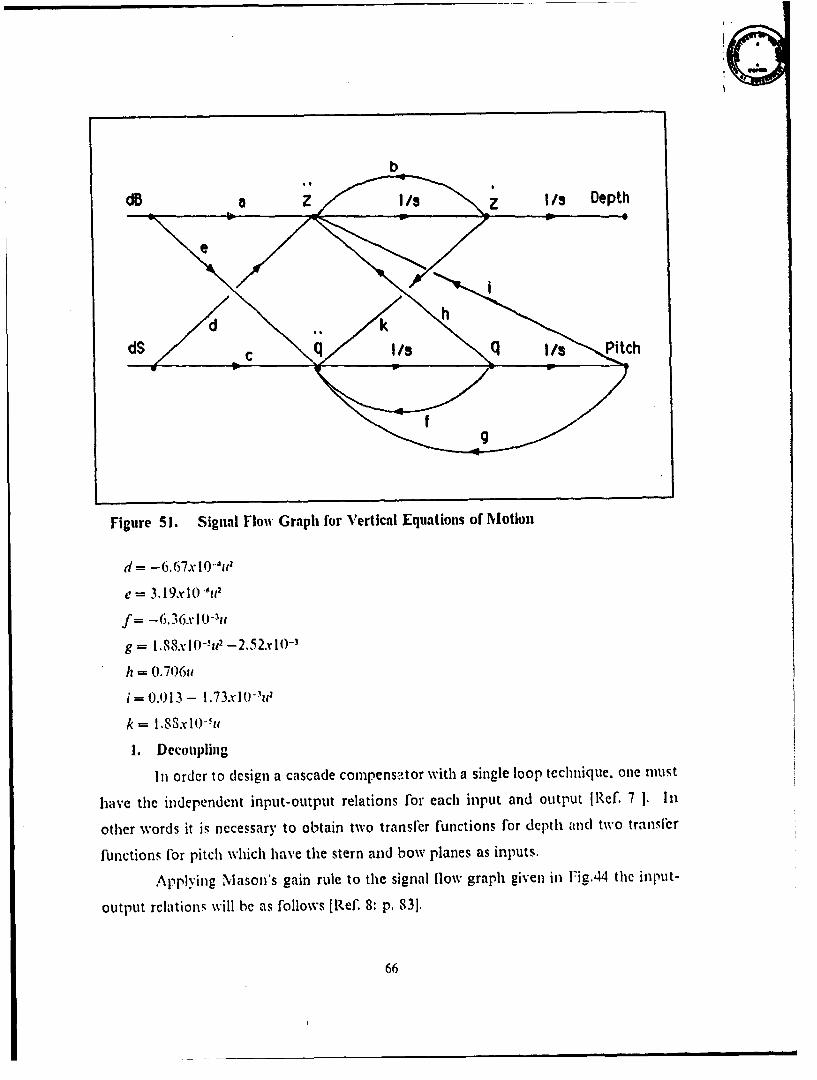
Figure 50. Cross-Coupling Elfect on Vertical Plane. Rudder - 35 Deg. U= 18 Kts. 64Figure 51. Signal Flow Graph lor Vertical Equations of Motion .............. 66

Figure 52. Cascade Compensated Control .Model for Vertical Motion ........... 70

Figure 53. Root Locus Plot lbor g,(s) ................................... 71Figure 54. Open Loop Bode Plot for g,,(s) .............................. 72

Figure 55. Root Locus Plot Ior g,(.s) .................................. 73

Figure 56. Open Loop Bode PNot for g,,(s) . ............................. 74Figzurc 57. Root Locus Plot fo." gkjs) .................................. 75

Figure 58. Open Loop Bode Plot for g(,s) ............................... 76

Figure 59. Root Locus Plot for g2,(s) .................................. 77

Figure 60. Open Loop Bode Plot for g2,1s) .............................. 78

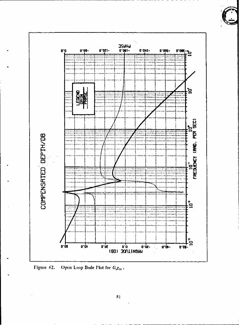
Figure 61. Root Locus Plot ior G,g, . . . . . . . . . . . . . . . . . . . . . . . . . . . . . . . . . . . sFigure 62. Open Loop Bode Plot for Ggt .. ............................. 81

Figure (3. Block Diagram for Compensated Linear Model in Vertical Motion .... 82

Figure 64. Compensated System Depth Response Z = 0.1, P = 1.0 ........... 86Fligure 65. Compensated System Depth Response KI = 0.015, K2 = 1.0 ....... 87Figure 66. Plane Angle Dellections for lirst and second Compensator ......... SS

viii

Figure 67. Compensated System Response to 100 ft. Depth Change .......... 89

Figure 68. Compensated System Pitch Response for Cormmianded Pitch = -. 5 Deg. 90

Figure 69. Compensated System Response to 10 ft. Depth Change U = 9 Kts.. 91

Figure 70. Compensated System Response to 100 ft. Depth Change U=9 Kts. 92

Figure 71. Compensated System Response to l0 ft. Depth Change U= 12 Kts. 93

Figure 72. Comprnsated System Response to 100 ft. Depth Change U= 12 Kts. 94

Figure 73. Compensated Systmi Response to 10 ft. Depth Change U-= IS Kts. 95

Figure 74. Compensated System Response to 100 ft. Depth Change U= 18 Kts. 96

Figure 75. Cascade Compensated Control Model for Horizontal Motion ....... 99

Figure 76. Signal Flow Graph for Horizontal Equations of Motion .......... 100

Figure 77. Root Locus Plot for EL ................................. 101

Figure.- 78. Open Loop Bode Plot for -... ............................. 102

Figure 79. Open Loop Bode Plot for GG, ............................. 104

Figure 80. Root Locus Plot Vor GG, ................................. 105

Figure 81. Block Diagram for Compensated Linear Model in Horizontal Motion 106

Figure 82. Yaw and Roll Respotnx,: ,o 10 Degree Course Change. No Limiter . 108Figure 83. Yaw and Roll Response to 15 Degree Course Change. With Limiter 109

Figure 84. Yaw and Roll Response to 90 Degree Course Change. U = 6 Kts.. 110

Figure 85. Yaw and Roll Response to 15 Degree Course Change. U = 10 Kts. IIl

Figure 86. Yaw and Roll Response t3 90 Degree Course Change. U = 10 Kts. 112

Figure 87. Yaw and Roll Response to 15 Degree Course Change. U = 15 Kts. 113




Figure 91. Compensated Submarine Depth Responses at 6 Kts .............. 121

Figure 92. Compensated Submarine Yaw Responses at 6 Kts ................ 122

Figure 93. Compensated Submarine Depth Responses at 10 Kts ............. 123

Figure 94. Compensated Submarine Yaw Responses at 10 Kts ............... 124

Figure 95. Deviations from the Conumanded Speed for Non-Linear Submarine . 125

FVigure 96. Cross-Coupling Effects flor the Non-Linear Submarine at 10 Kts ... 126

Figure 97. Course and Depth Change Conunanded at the Same Time UC= 10

Kts .................................................. 1 27Figure 98. Roll. Pitch and Speed Response for Multi-Manevuer Submarine ... 128

Figure 99. Depth and Pitcli Response for Fixed Rudder Comnmands U = 12 Kts. 129Figure 100. Compensated Submarine Yaw Responses at 15 Kts............. 130

ix

Figure 101. Compensated Submarine Depth Responses at 15 Kts ............ 131Figure 102. Depth Change with 5 Deg. Down Pitch Angle for Non-Linear Sub. . 132Figure 103. Compensated Submarine Yaw Responses at 20 Kts ............. 133Figure 104. Compensated Submarinc Depth Responses at 20 Kts ............ 134Figure 105. Compensated Submarine Pitch Response to Depth Change Com-

m ands ............................................... 135

x

ACKNOWLEDGEMENTS

The author wishes to express his sincerc appreciation to Dr. George J. Thaler forthe guidance, assistance and continuous encouragement which he provided during thepursuit of this study. The author would also like to express his appreciation to LTJGLevent Korkinaz from Turkish Navy for his valuable assistance.

xi

1. INTRODUCTION

Since they are operated in three dimensions and because of their different body

structure and operational conditions, submarines always present a great challange for

automatic control engineers. Especially flor submarines with extremely high underwater

speeds, it is very important to have automatic controls which can be used effectively.In this study, using the equations of motions in six degrees of freedom which were

developed by Naval Ship Research and Development Center (NSRDC), a linearizedsubmarine model was derived for both horizontal and vertical motions. It was obvious

that working with a linear model is much simpler then with a complete nonlinear model.

Also the automatic control system design procedures which are used in this study require

a linear model for decoupling. Even though the linearized model does not introduce a

cross-coupling effect between horizontal and vertical motion, as would a real submarine,it works in almost the same way the nonlinear model does.

In designing an automatic controller flor both vertical and horizontal motions, a

MI'lO ( Multi-input Muihi-output ) system representing the submarine, has to be in-

vestigated. Inputs are propeller which creates the forward speed, rudder for horizontal

motion, and the bow and stern planes !or vertical motion. The outputs are the three

speed components u, w, v and roll, yaw, pitch angles around three axes of the sub.marine.

Also a ballast system can be used to maneuver the submarine but it is not included in

this study assuming the submarine is always in trim.

The pitch and yaw angles and the depth have the main importance for maneuvering

a submerged submarine. Therefore the automatic control system is designed to control

these three states.

After obtaining valid linear models for both horizontal and vertical motions, the

method of the automatic control design has to be chosen. One of the most popular de-

sign method is optimal control theory but it requires fIeedback of both position and rate

information. This inlormation is available for submarines which are equipped with an

inertial guidance system. For the small coastal submarines which do not have an inertialguidance system, a different design approach must be carried out. A possible way would

be the design of cascaded compensators using only position ( such as depth ) feedback."There is always a cross-coupling effet between vertical and horizontal motion in a

submerged submarine which is also called a squatting effect. The cross-coupling effect

is simply the rudder effect on vertical plane which makes the submarine pitch up and

change depth when a rudder angle is applied. The cross-coupling ellect is also investi-

gated in this study.

2i

II. EQUATIONS OF MOTIONS IN SIX DEGREES OF FREEDOM

A. BACKGROUNDWith diving capability, submarines differ from surface ships. They also have com-

pletely diflerent hull structures, hydrodynamic specifications and relatively complex

control and stability problems. A submarine can be operated in all six degrees of free-

dora. To maneuver usually three sets of plane surfaces, the propulsion system consisting

of one or two propellers, and a ballast system consisting of two or three ballast tanks for

dill'erent type of submarines are used.

To control horizontal motion the submarine has a usual rudder such as surface ships

do. But in vertical motion, a submerged submarine needs at least one more control sur-face to maintain the desired depth and pitch angle.A classic submarine has bow planes,

which can be used to keep ordered depth, and stern planes, which can be used to tilt the

submarine to an ordered pitch angle. Depending on the submarines's speed and condi-

tion these planes can have an appreciable interaction.

Modern submarines usually have bow planes on their sails, which are called

fairwater planes. I lowever, high underwater speeds reduce the necessity of' bowplanes.

It is possible to keep ordered depth without using bow planes while operating with

higher underwater speeds. Since the numbers presented by NSRDC [Ref. 1: p. 88] are for

an American submarine, bow and flairwater planes were both considered in this study.

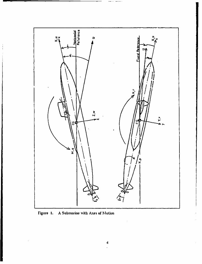
An illustrative picture of a submarine with axes, velocity and plane definitions is

given it Fig.1. The arrows are pointed in the positive motion direction.This coordinate

system is the right hand orthogonal system which is fixed in the submarine aud moves

with it. The origin of the coordinates is located at the center of gravity with x-axis along

the center plane. The positive x direction is forward, the positive y direction is horizon-

tally to the right, and the positive z direction is down. [Ref. 2: p. 43S]

The heading of the submarine is the direction of its x-axis, and this is measured as

an angle with respect to the geographic coordinate system. The heading angle, also

called the yaw angle, is defined to be the angle between the direction of the ships x-axis

and the direction of the x-axis of the geographic coordinate system. The symbol used for

the yaw angle is •,.

3

xt

04e

FeI

= I I°

N *, •

Filgure 1. A Subnlarine iiltl A~xes of Motioli

4

The pitch angle of the ship is the rotation around its y-axis. It is defined to be the

angle between the direction of the ships x-axis and the horizontal ref'erence line. Thesymbol used for the yaw angle is 0

"T[he roll angle of the submarine is the rotation around its x-axis. It is measured from

the vertical reference to the direction of the submarine z-axis. The symbol used for the

roll angle is 0.Velocities for the x, y and z directions are u, v and w respectively, which can be

called velocity components of linear velocity of body axes relative to an earth-fixed axis

system.

Definitions for all symbols used in this study are given in Appendix A.

B. DERIVATION OF THE LINEARIZED MODEL

The equations of motion are derived by sunmming the applicable forces and moment.s

in each degree of freedom: surge(x), sway(y), heave(z), roll(o), pitch(0) and yaw(qI).

Ref erence I presents the standard sets of' equations of motion developed [or submarine

motion studies by NSRDC. These equations are general enough io simulate the trajec-

tories and responses or submarines in the six degrees c" freedom resulting from various

types of maneuvers. They simulate motion of a given ship design upon insertion of the

nondimensionalizcu hydrodynamic coeflicients developed for that particular design. In

addition values must be supplied for propulsion force and rudder and diving plane an-

gles. A complete set of' hydrodynanic coefficients and other required data used in this

thesis is given on Appendix 13.

The derivation of equations of motions in six degrees of freedom which are to be

linearized, was discussed in several earlier studies. [Ref. 3 , Ref. 4 .1 The authors were

satisfied that these equations are valid and can simulate a submarine's motion ell'cc-

tively.

I. Assumptions

Forward speed can be taken as constant. Linearizing about the axial speed,u,

which affects nearly every term in the standard equations, could be very complex, so the

forward speed was assumed to be constant. This also reduces the degrees of freedom to

live.

Roll angle is assumed to be small. Under normal circumtances in submarine

maneuvering, the roll angle usually stays within +5'. Large roll angles arc only caused

by high speed plus hard over rudder. Therellore, the roll angle can be neglected.

Cross-products of incrtia can be neglected. This assumption is common to all

submarine simulations because the hull and interior layout of submarines is approxi-

mately symmetric.

All terms including 11, can be discarded. Since it is assumed that the submarineis in trim, weight of water blown from a particular ballast tank, RW., must equal zero.

.All terms involving nonlinearity are neglected.Vertical motion is decoupled from horizontal motion. As a result of the first five

assumptions it aiso has to be assumed that there is no coupling between vertical and

horizontal motion.

2. Derivation of the linear equations of Motion

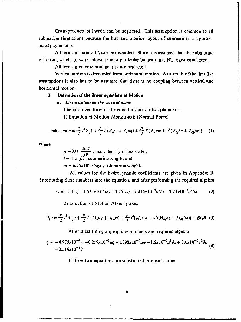
a. Lhtearization on the vertical planeThe linearized fbrm of the equations on vertical plane are:

1) Equation of' Motion Along z-axis (Normal Force):

nii -- unq -L--'Z 4 6+ - L- I(Z,-, + . q) + 2 l(ZWuw + u 2(Z5s5s + Zab6b)) (1)

where

p = 2.0 ,mass density of sea water,Pt3

1 = 415 ji. , submarine length, and

in = 6.25xl0• shlgs , submarine weight.

All values for the hydrodynanfic coefficients are given in Appendix B.Substituting these numbers into the equation, and after perfornming the required algebra

i' = -5.1 14 -l.632xl-S 3 uw +0.261uq -7.416xl0-4u 22s -3.71xlOau 26b (2)

2) Equation of Motion About v-axis:

1,4 = 2- ISA$ + -L tIquq + "4tA) + -2-. ij3(Mwuw + U2(M,',65s + ili6b6 b)) + BzBO (3)

After substituting appropriate numbers and required algebra

4= -4.975xl'0vi.-6.219X.l0- 3 uq +l.798x1O- 5uw -l.5xlO-Su 2 6s + 3.OxlO- 6u26b+2.516x10_3 0 (4)

If these two equations are substituted into each other

6

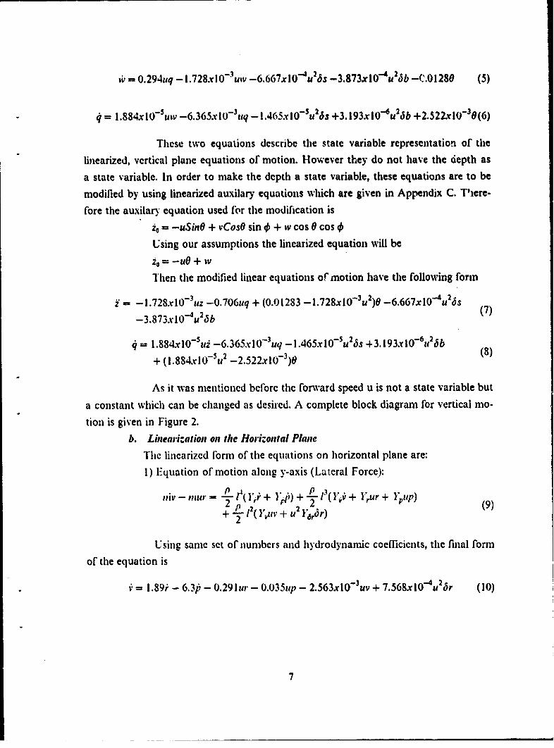
wi - 0.294uq - 1.728x10 uv -6.66 7x 10-4u s -3.873xO1'u 25b -C.01280 (5)

= 1.884x10- 5 uw -6.365xlO-3 uq - 1.465x10-Su26s +3.193xlO0 6 u2 6b +2.522rl0- 3 0(6)

These two equations describe the state variable representation of the

linearized, vertical plane equations of motion. However they do not have the depth as

a state variable. In order to make the depth a state variable, these equations are to be

modified by using linearized auxilary equations which are given in Appendix C. There-

fore the auxilary equation used for the modification is

zo - -uSinO + XCosO sin 0 + w cos 0 cos 4•Using our assumptions the linearized equation will be

ic = -uO + w

Then the modified linear equations of motion have the following form

i= -1.728x.1(-3uz -0.706uq + (0.0 1283 -1.728x10- 3u2)0 -6.667x 10- 4 u216

-3.873x lO u'2 b (7)

- 1.884xI 0-Sd -6.365x10-3uq - 1.465x 10-5u 25s + 3.193x 10-5u 26b

+ (l.884x.1-Su2 -2.522xl0_ 3)0 (8)

As it was mentioned before the forward speed u is not a state variable but

a constant which can be changed as desired. A complete block diagram for vertical mo-

tion is given in Figure 2.b. Linearization on the Horizontal Plane

The linearized form of the equations on horizontal plane are:

1) Equation of motion along y-axis (Lateral Force):nP -M11 e, PII

,,iv - ,,i,, = 23 F~( };. ; • + + t(o+ },r + }'Pp)-- -i " -+ j + + Y ur + 1 tip)

+ j. 2 Y~u + U2 Y rP

Using same set of numbers and hydrodynamic coefficients, the final form

or the equation is

i= 1.89i - 6 .3p - 0.29 1ur - 0.035up - 2.563x10-3 uv + 7.568xlO-4u 26r (10)

7

db -4 2-3-I 3.87x 10 u 1.73x 1 0 u

6.67x10 u

-0.706u 1.88x 10 u-

S.0 13-1.73x 10u

•--3.19xl0 u +,+

; I 1.465x 10 u_•+

6.6x1 -5 2 -3&365x I 0 u1.88x 1 0 u -2.52x 1 0-

Figure 2. Block Diagram for the Linearized Model oin the Vertical Plane

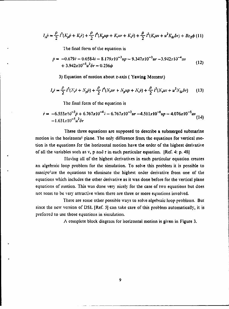
.p l-(Kril + Kr) + "( .(Kup + Kur + Kjy) + •',",uv + u2'K6,r) + Bz•, (11)

The final form of the equation is

p - -0.679W - 0.0584h' - 8.179x lO-3up - 9.347x10-3ur -3.942xl.e-4v

+ 3.942xlO-Su26r - 0.2360 (12)

3) Equation of motion about z-axis ( Yawing Moment)

I L •1("vr•+ N•)) + 2- e(Nur *_ ,;UP + ,vi) + _L -1(AVuv + u 2lyNrbr) (13)

The final fborm of the equation is

i - -6.553xh0- 3 /• + 6.767x1,O' - 6.767xO1-3ur -4.51 x1O- 6up - 4.076xlO-Suv- 1.631ix'10-5u 2jr (4

These three equations are supposed to describe a submerged submarinemotion in the horizontal plane. The only dil•hrence from the equations for vertical mo-tion is the equations for the horizontal motion have the order of the highest derivativeof all the variables such as v, p and r in each particular equation. [Ref. 4: p. 481

I laving all of the highest derivatives in each particular equation createsan algebraic loop problem for the simulation. To solve this problem it is possible tomanipulate the equations to elininate the highest order derivative from one of theequations which includes the other derivative as it was done before for the vertical plane

equations of motion. This was done very nicely for the case of two equations but does

not seem to be very attractive when there are three or more equations involved.

There are some other possible ways to solve algebraic loop problems. But

since the new version of DSL [Ref 5] can take care of this problem automatically, it is

preferred to use those equations in simulation.

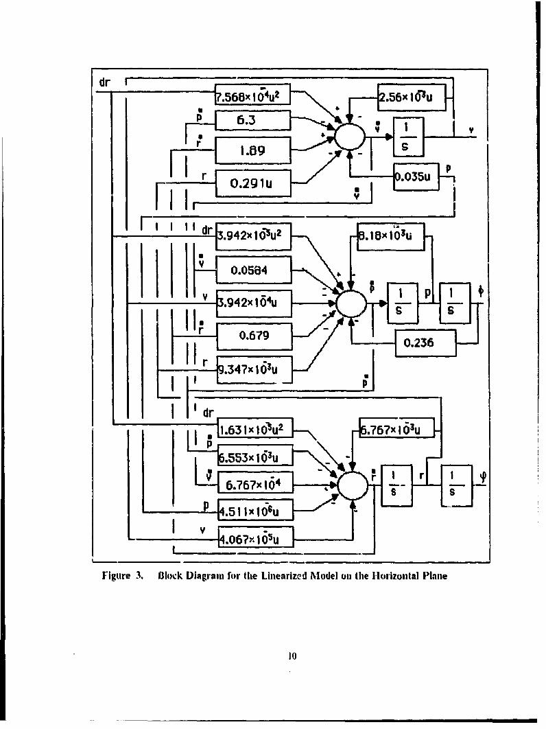
A complete block diagram for horizontal motion is given in Figure 3.

rl~I rI o.291,. *- 'I , o .

I dr

[p 6.3i6,!6,

Figure 3. fluiwk D ia grlanm for tile Linearized Mlodel oli the l-|O i Izonital P hine

l0

N2

v

C. VALIDATION OF LINEAR MODEL

The objective of this section is to compare the dynamics of the standard model witethe derived linear model in both vertical and horizontal planes.

In order to compare both models they should be in the same initial state and bothmodels have to be in trim. in trim has the meaning that the submarine maintains depthat a given speed with the desired pitch angle without using bow or stern planes. Whenmaking linearizing assumptions the terms which are related to trim are already ignored.Therefore the linearized model will be in trim at all times. Because of the submarine hulland sail structure it is required to adjust ballast tanks for given speed. The correctionsfor trim which are used in the simulation for this study are obtained from an earlier

thesis study. [Rcf. 6: p. 1841"1To validate the linear model it is preferred to obtain both the initial condition and

forced response in order to make sure that the linear model is working properly.1. Validation of Linear Model on Vertical Plane

a. Initial Condition Response

It was expected that for small perturbations the deviations between models

should be small. Therefore initial conditions of 5. in pitch were tested first. For the linearmodel it is also required to give an initial value for depth change which was defined as:

z = -uSin 0

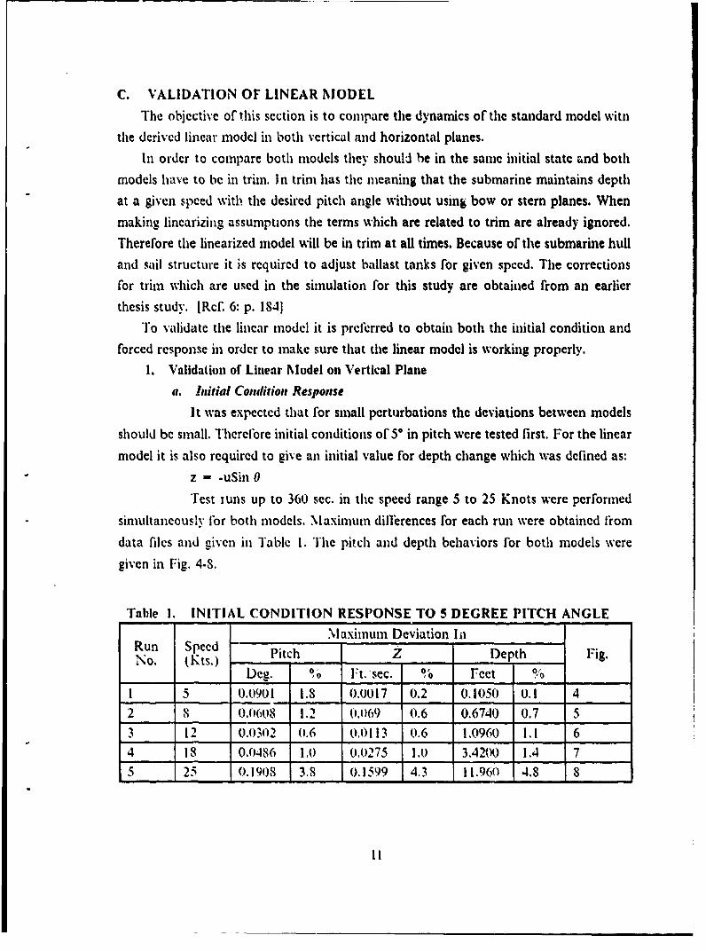
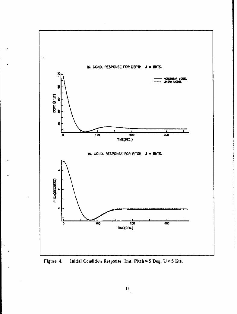
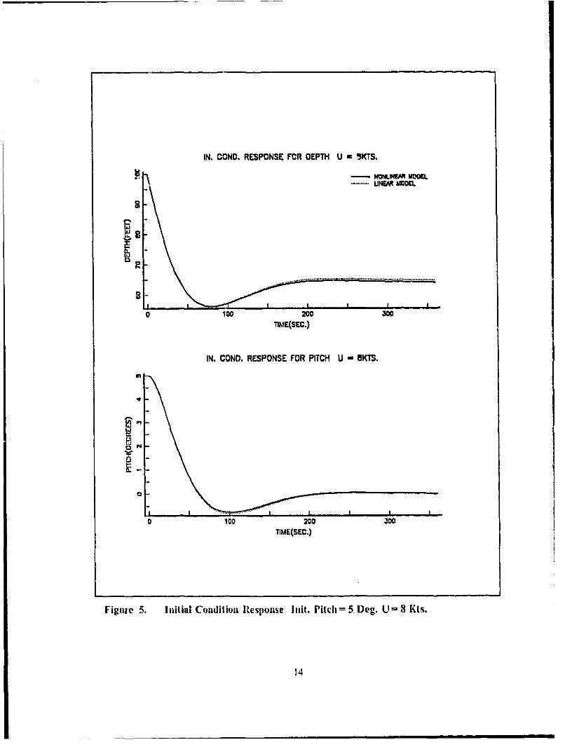
Test iuns up to 360 sec. in the speed range 5 to 25 Knots were performed

simultaneously for both models. Maximum differences for each run were obtained from

data files and given in Table I. The pitch and depth behaviors for both models were

given in Fig. 4-S.

Table 1. INITIAL CONDITION RESPONSE TO 5 DEGREE PITCH ANGLEMaximum Deviation In

Run Speed - Pitch Z Depth Fig.No. (Kts.)

Deg. 0% F-t. sec. % Feet 01 5 0.0901 1.8 0.0017 0.2 0.1050 0.1 42 8 0,0608 1.2 (0.069 0.6 0.6740 0.7 53 12 0.0302 (0.6 0.0113 0.6 1.0960 I. 1 64 18 0.0486 1.0 0.0275 1.0 3.4200 1.4 75 25 0.1908 3.8 0.1599 4.3 11.960 4.8 8

11

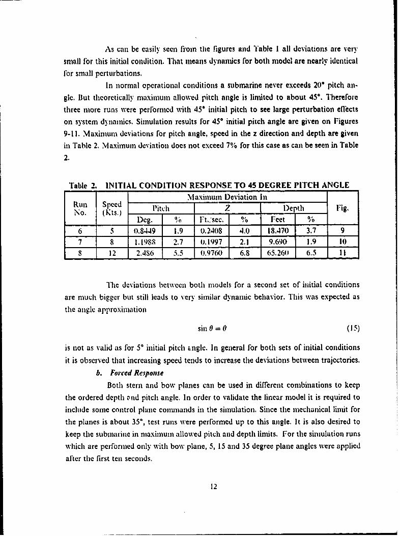
As can be easily seen from the figures and Table I all deviations are very

small for this initial condition. That means dynamics for both model are nearly identical

for small perturbations.

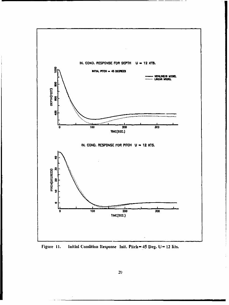
In normal operational conditions a submarine never exceeds 20" pitch an-

gle. But theoretically maximum allowed pitch angle is limited to about 45*. Therefore

three more runs were perlbrmcd with 45° initial pitch to see large perturbation eftcts

on system d~ namfics. Simulation results for 45° initial pitch angle are given on Figures

9-11. Maximum deviations for pitch angle, speed in the z direction and depth are given

in Table 2. Maximum deviation does not exceed 7% for this case as can be seen in Table

2.

Table 2. INITIAL CONDITION RESPONSE TO 45 DEGREE PITCH ANGLE

Maximum Deviation InRun Speed Pitch 7 Depth IFig.No. (Kts.)

D__ ieg. % Ft.'sec. % Feet 0_6 5 0.8449 1.9 0.2408 4.0 18.470 3.7 9

7 8 1.1988 2.7 0.1997 2.1 9.690 1.9 iI)S 12 2.486 S.5 0.9760 6.8 65.260 6.5 11

The deviations between both models for a second set of initial conditions

are much bigger but still leads to very similar dynamic behavior. This was expected as

the angle approximation

sin 0 = 0 (15)

is not as valid as for 5* initial pitch zngle. In general for both sets of initial conditions

it is observed that increasing speed tends to increase the deviations between trajectories.

b. Forced Response

Both stern and bow planes can be used in different combinations to keep

the ordered depth and pitch angle. In order to validate the linear model it is required to

include some control plane conunands in the simulation. Since the mechanical limit for

the planes is about 35*, test runs were performed up to this angle. It is also desired to

keep the submarine in maximum allowed pitch and depth limits. For the simulation runs

which are performed only with bow plane, 5, 15 and 35 degree plane angles were applied

after the first ten seconds.

12

IN. COND. RESPONSE FOR DEPTH U - 5KtS.

- N0NUMOOEL- LFMR MOM

i.

0 100 200 300TIME(SEC.)

IN. COND. RESPONSE FOR PITCH U -5KtS.

0 O00 200 300TIME(SEC.)

Figure 4. Initial CoNdition Response Fit. Pltch 5 Deg. U 5 Tis.

13

IN. COND. RESPONSE FCR DEPTH U a 1KTS.

-NONLINEAR WMO6........... IUNEAR MODEL

010O0 200 300

IN. COND. RESPONSE FOR PITCH U "KTS.

TIME(SEC.)

Figure 5. lnitial Condition flesponse lmit. I'itch = 5. Deg. U S K lts.

14

/ IN. COND. RESPONSE FOR DEPTH U -1 2KTS.

/

B - ~NOUE.AR M000.......UNEAR MODEL.

/

............................. ..................... .............

0 100 200 300TIME(SEC.)

IN. COND. RESPONSE FOR PITCH U - 12KTS.

in

C.)

a -

0 100 200 300TIME(SEC.)

Fitire 6. I nitial Condition Response nit. Pitch 5 Deg. U 12 Kts.

15

IN. COND. RESPONSE FOR DEPTH U - 18 KTS.

- NONRNL.AR MODEL. . .. .........UNEAR MOOEL

i2

L-

0 100 200 300TIME(SEC.)

IN. COND. RESPONSE FOR PITCH U - 18 KTS.

4.

V.

0 100 200 3o0

TIME(SEC.)

Figure 7. Initial Condition Response hilt. Pitch= 5 Deg. U- 1S Kts.

16

IN. COND. RESPONSE FOR DEPTH U " 25 KTS.

- NONLINFAR MODEl

S........... UNE.AR MODEL

... ............... ,r .................UNA O~.

I .. ...... ............. ....................... .

0 100 200 300TIME(SEC.)


im

0 100 200 300TIME(SEC.)

Figure 8. Initial Condition Response Init. Pitch= 5. Deg. U= 25 Kts.

17

IN. COND. RESPONSE FOR DEPTH U 5 3 KIS.

INm. PITCH -45 DEC]REE

- NONUN.REM MODEL. *ULINEAR MODEL

....... .............. ,°................. 0°..........,........ . .. °..°.0.°........... ...... °°. ....... .. °..°............ .. °...,.

100 200 300TIME(SEC.)

IN. COND. RESPONSE FOR PITCH U 5 5 KTS.

.... ..

0 100 200 300

TIIE(SEC.)

Figure 9. Initial Condition Response hInt. Pitch= 45 Deg. U= 5 Kts.

18

IN. COND. RESPONSE FOR DEPTH U - 8 KTIS.

vINfrT PrfCIH - 45 DECRE-- NONLINEARMOS...... .... LINEAR MODEL.

0100 200 300

1nME(SEC.)

IN. COND. RESPONSE FOR PITCH U a 8 KTS.

0.-0.---...

.... ..... ................0 100 200 300

TIIAE(SEC.)

Figure 10. Initial Condition Response lnit. Pitch=45 Deg. U=8 Kts.

19

IN. COND. RESPONSE FOR DEPTH U - 12 KTS.

WNfnfL PITCH - 45 DEOlM

- NONUN.iR MOUM.*........... LN a MOGU.

... ..

""..... ...... ..... ........... - i

0 100 200 3coflME(SEC.)


0-R

0 I00 200 300TIME(SEC.)

Figure Ii. Initial Condition Response Init. Pitch=-45 Dog. U = 12 Kts.

20

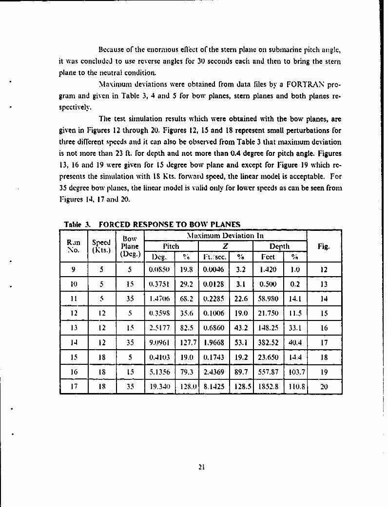
Because of the enormous effect of the stern plane on submarine pitch angle,

it was concluded to use reverse angles ror 30 seconds each and then to bring the stern

plane to the neutral condition.

Maximum deviations were obtained rrom data files by a FORTRAN pro-gram and given in Table 3, 4 and 5 for bow planes, stern planes and both planes re-

spectively.

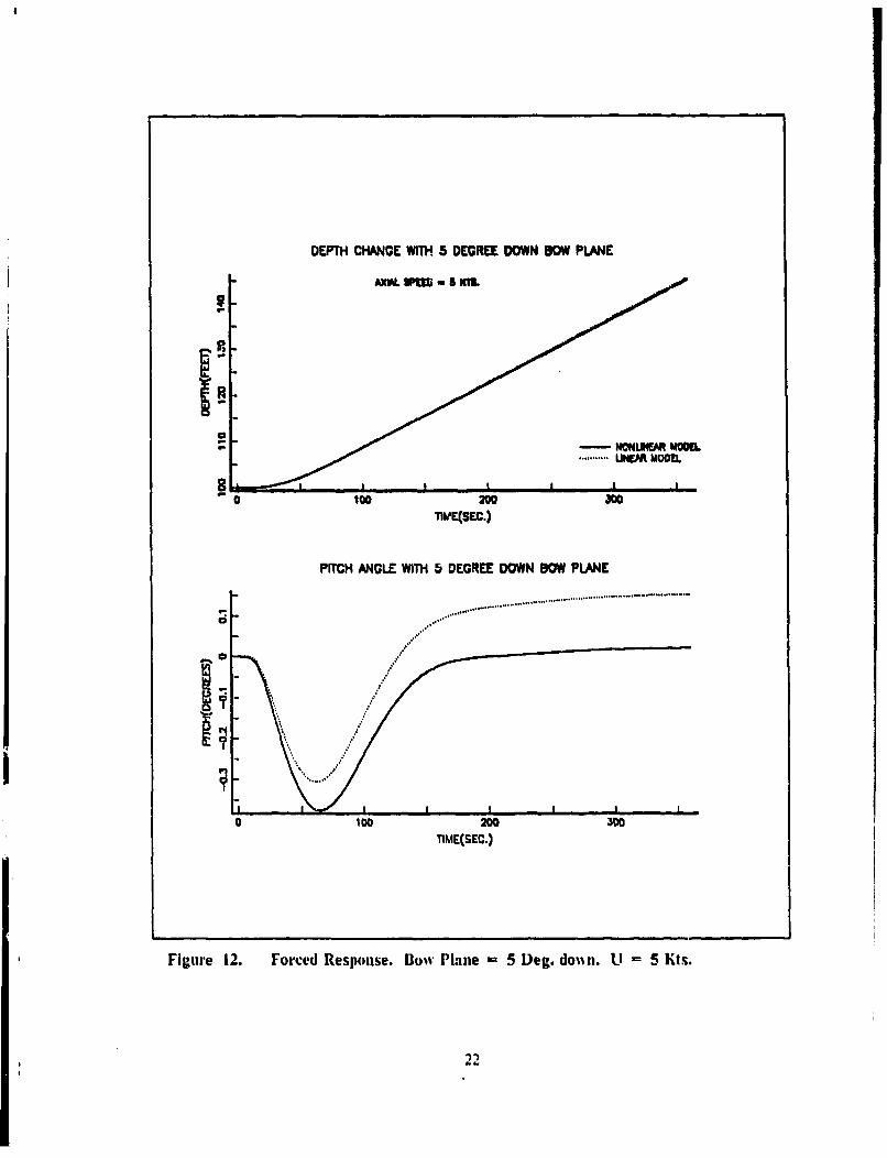
The test simulation results which were obtained with the bow planes, are

given in Figures 12 through 20. Figures 12, 15 and 18 represent small perturbations for

three different speeds and it can also be observed from Table 3 that maximum deviation

is not more than 23 ft. for depth and not more than 0.4 degree for pitch angle. Figures

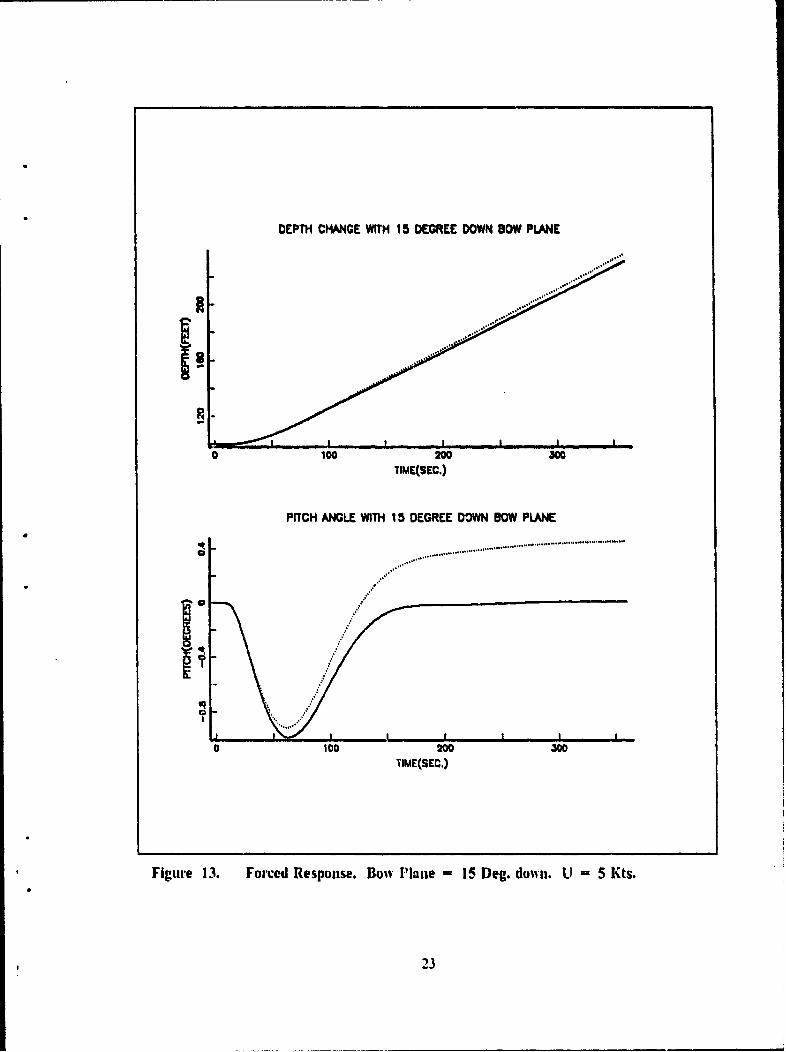
13, 16 and 19 were given for 15 degree bow plane and except for Figure 19 which re-

presents the simulation with IS Kts. florward speed, the linear model is acceptable. For

35 degree bow planes, the linear model is valid only for lower speeds as can be seen from

Figures 14, 17 and 20.

Table 3. FORCED RESPONSE TO BOW PLANES

d Bow .laximum Deviation InRNn Speed Plane Pitch Z Depth Fig.No. (Kts.) (Deg.) meg. % 0 Ft./sec. % Feet 6

9 5 5 0.8,50 19.8 0.0046 3.2 1.420 1.0 12

10 5 15 0.3751 29.2 0.0128 3.1 0.5(X) 0.2 13

11 5 35 1.4706 68.2 0.2285 22.6 58.980 14.1 14

12 12 5 0.3598 35.6 0.1006 19.0 21.750 11.5 15

13 12 15 2.5177 82.5 0.6800 43.2 148.25 33.1 16

14 12 35 9.1961 127.7 1.9668 53.1 382.52 40.4 17

15 18 5 0.4103 19.0 1 0.1743 19.2 23.650 14.4 18

16 Is 15 5.1356 79.3 2.4369 89.7 557.87 103.7 19

17 Is 35 19.340 128.0 8.1425 128.5 1852.8 110.8 20

21

DEPTH CHANGE WITH 5 DEGREE DOWN BOW PLANE

AI -a m

........... UNE MODEL

0 00 200 300flh'E(SEC.)

PITCH ANGLE WITH 5 DEGREE DOWN DOW PLANE

S,,,o,°,°.o,,°,,,,...,•..°...°..... .... °. . .......... ....... . ,...°.o..-"-°•'"*

.•°"-- ---------

I I I .I .

0 100 200 300

TIME(SEC.)

Figure 12. Forced Response. Bow Plane = 5 Deg. domil. U - 5 lits.

22

DEPTH CHANGE WITH 15 DEGREE DOWN BOW PLANE

i,

0 100 200 300TIME(SEC.)

PITCH ANGLE WITH 15 DEGREE DOWN BOW PLANE

. . . .

C;

0 100 200 300TIME(SEC.)

Figure 13. Forced Response. Bow Plane = 15 Deg. dow-n. U = 5 Kts.

23

FORCED RESPONSE WITH 35 DEG. BOW PLANE

AXIAL SPEED U - 5 KTS.

p -

SNoNUNVR.g ¥mlf.. , ........... UINF.M MODEL

0 1oo 200 300liME (SEC.)

0 100 200 300"TIME (SEC.)

Figure 14. Forced Response. Bow Plane - 35 Deg. down. U - 5 Kts.

24

FORCED RESPONSE WITH 5 DEG. DOWN BOW PLANEAXIAL SPEED U - 12 KTS.

I

0 100 200 300TiME (sEC.)

gurce U 2o Pl 5 d U

2.-.5....L - -I - I I - I0 100 200 300

TIME (SEC.)

Figure 15. Forced Response. Bow Plane =5 Deg. down. U =12 Kts.

25

FORCED RESPONSE WITH 15 DEG. DOWN 80W PLANE

AXIAL SPEED U - 12 KIS.

-- NONLINEAR MODEL..........................LNEAR MODEL

0 100 200 300

TIME (SEC.)

.........-"........... .... ..............

0 100 200 300

TIME (SEC.)

Figure 16. Forced Response. D.ow PlIne = 15 Deg. down. U= 12 M~s.

26

FORCED RESPONSE WITH 35 DEG. DOWN BOW PLANE


gi

...... ...... ... . ... . ..... .............. . . ...........

.. * - NONUNF.AR MODEL

UNrW MOs.ci

0 100 200 3

0 100 200 300TIME (SEC.)

Figure 17. Forced Response. Bowv Plane =35 Deg. down. U =12 lits.

27

FORCED RESPONSE WITH 5 DEC. DOWN BOW PLANE

0 100 200 300"TIME (SEC.)

- NQNUNEAR MODIE............ UNEAR MODEL

44 ..... .... ............

" .,....f . , , , I I I

0 100 200 .300TIME (SEC.)

Figure 18. Forced Response. Bow Plane 5 Deg. doisn. U = 18 Kts.

2S


AXIAL SPEED U = 13 KTS.

~.... -NONUINVA MODEL........................UNWA MODEL.

0100 200 .. 00 "

TIME (SEC.)

. . . . . ... ..................... . ......... . ............ ......

TIME (SEC.)

F igure 19. rorced Response. Bow Plane =15 Deg. dowin. U =18 Kts.

29


0- AXIAL SPEED U - 18 KTS.

-N0NUPAR MOM9.......... ... .... .......... WEAR MODE

SI......... ........... ........ I ....

0 100 200 300TIME (SEC.)

........... . .......................... . . ....

I...0,

01lo 200 ,300

TIME (SEC.)

Figure 20. Forced Response. Bow Plane 35 Deg. down.. U 18 KIs.

30

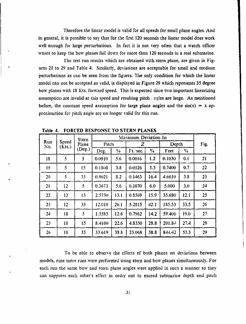
Therefore the linear model is valid for all speeds for small plane angles. And

in general, it is possible to say that for the first 120 seconds the linear model does work

well enough for large perturbations. In fact it is not very often that a watch officer

wants to keep the bow planes full down for more than 120 seconds in a real submarine.

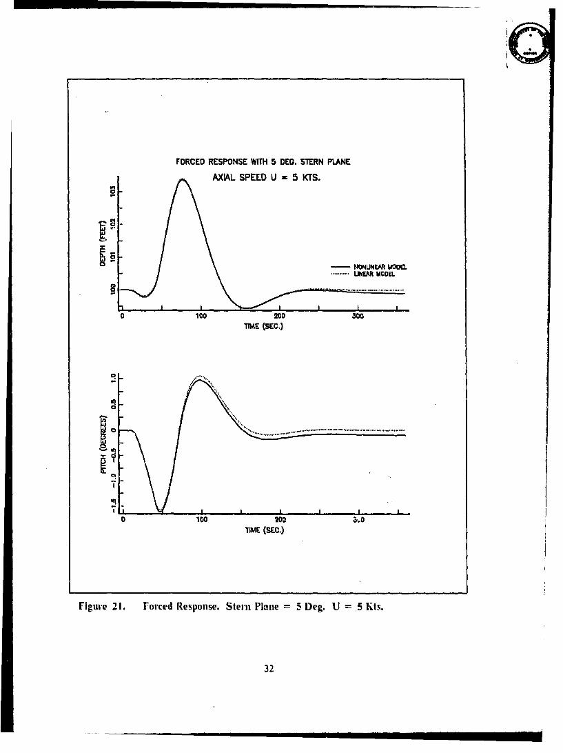
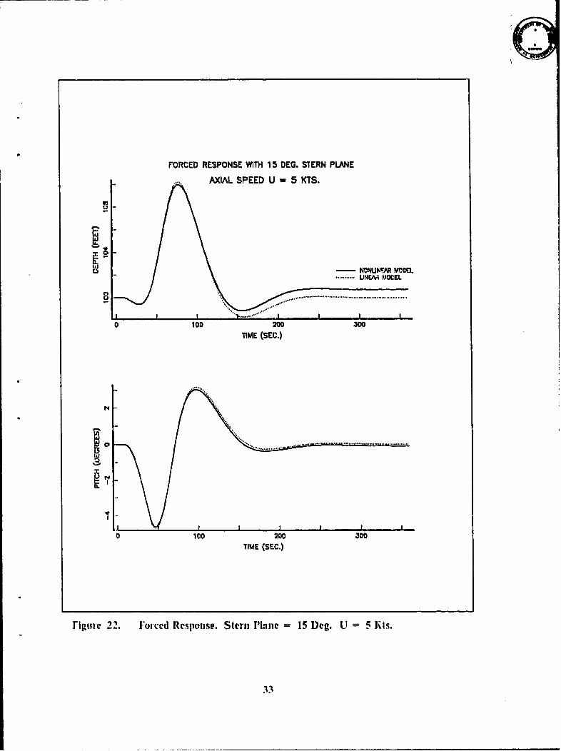
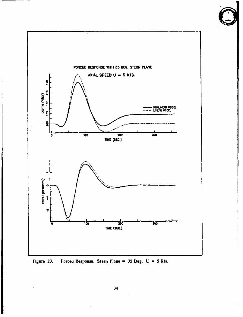
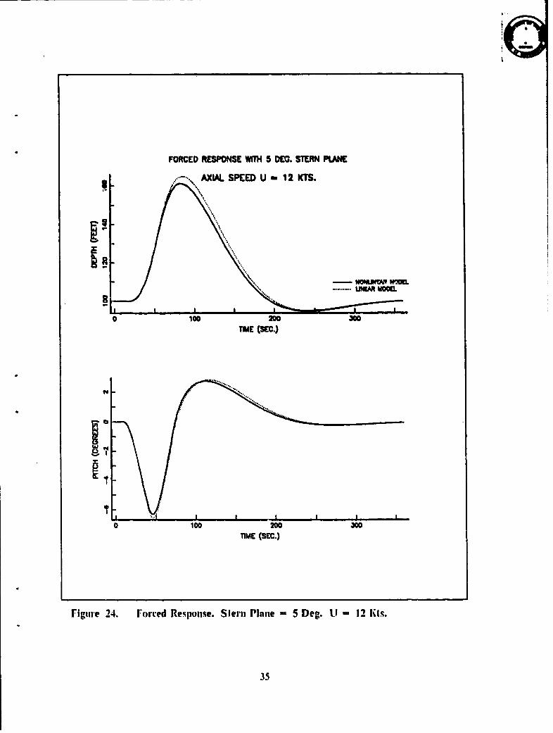
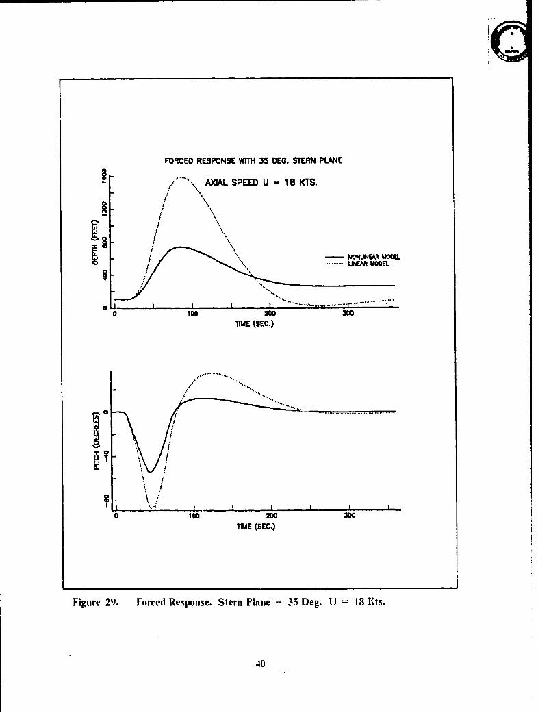
The test run results which are obtained with stern plane, are given in Fig-

ures 21 to 29 and Table 4. Similarly, deviations are acceptable for small and medium

perturbations as can be seen from the figures. The only condition for which the linear

model can not be accepted as valid, is displayed in Figure 29 which represents 35 degree

bow planes with 18 Kts. forward speed. This is expected since two important linearizing

assumption are invalid at this speed and resulting pitch .,ngles are large. As mentioned

before, the constant speed assumption for large plane angles and the sin(x) = x ap-

proximation for pitch angle are no longer valid for this run.

Table 4. FORCED RESPONSE TO STERN PLANES

Run Speed Stern Maxinmum Deviation InRN Spe Plane Pitch Z Depth Fig.No. (Kts.) (Deg.) Deg. % Ft..'sec. I o Feet

Is1 5 5 0.0910 5.6 0.0016 1.2 0.1030 0.1 21

19 5 15 0.1808 3.8 0.0126 3.3 0.7400 0.7 22

20 5 35 0.9021 8.2 0.1463 16.4 4.6610 3.8 23

21 12 5 0.3673 5.6 0.1070 6.0 5.000 3.0 24

22 12 15 2.5750 13.1 0.8569 15.9 35.680 12.1 25

23 12 35 12.010 26.1 5.2815 42.1 185.53 33.5 26

24 18 5 1.5585 12.6 0.7962 14.2 59.406 19.0 27

25 18 15 8.4160 22.6 4.8350 28.8 201.8J 27.4 28

26 18 35 33,619 38.8 23.068 58.8 844.42 53.3 29

To be able to observe the efrccts of both planes on deviations between

models, nine more runs were performed using stern and bow planes simultaneously. For

each run the same bow and stern plane angles were applied in such a manner so they

can suppress each other's effect in order not to exceed submarine depth and pitch

31

FORCED RESPONSE WITH 5 DEG. STERN PLANE


MN~fUNEAM MOM=S........... LINAR MODEL

0 100 200 300TIME (SEC.)

I ' " .., ..., , .....,................................... ........ : .... ....... .. . .. ... ..... ... ..

0

0 100 200 •,.0

TIME (SEC.)

Figure 21. Forced Response. Stern Plane 5 Deg. U = .5 Kts.

32


AXIAL SPEED U -5 KTS.

• -'• •''" • .................................. L14 ..................

l I I "'1 ..... • .. .... . .,......

0 100) 200

300

TIME (SEC.)

U,',

0100

200 300

TIME (SEC.)

Figure 22. Forced Response. Stern Pline -- 15 Deg. U = 5 Ihts.

33


AXIAL SPEED U - 5 KTS./ '.

-WONLJHEMR MOCEL

......................... WJ .............

I.I I ..I" ....... I.0 loo 200 300

71ME (SEC.)

'II-

0 lOO 200 300TIME (SEC.)

Figure 23. Forced Response. Sernl Plane = 35 Deg. U = 5 lit.

34

*% %

I

S/ ....... _- . s0S4Uu -A W 3r s

* UNEM MDCC.

I/4S...... .... UNE R m o

TIM (SEC.)

I .pII

0 100 200 300TIME (SEC.)

Figure 24. Forced Response. Slern Plane - 5 Deg. U - 12 lts.

35

a

FORCED RESPONSE WITH 15 DEC. STERN PLAE

....... .AXIAL SPEED U . 12 KTS.

/

-r"\'\,,m

.... ... ....... •

0 100 2300 30o

TIME (SEC.)

rigure 25. Forced Response. Stern Plane - 15 Deg. U -12 Kts.

36

FORCED RESPONSE WITH 35 DEC. STERN PLANEAXI...AL SPEE U - 12 KT.

. ............. .... .. .

o 100 200 300"TIME (SEC.)

A

I II I I pI

0 100 200 300

TIME (SEC.)

Figure 26. Forced Response. Stern Plane - 35 Deg. U - 12 lts.

37


. ...... AXIAL SPEED U -18 K'S.

• •. ,........... IJNMR VMO L8,- .." ........°.,.. o. . .. . ............. + .o .o........ ''' "

0 100 209 300TIME (SEC.)

.. ........ ......... . .... ....... .................~0

IQ %

0 100 200 300TIME (SEC.)

Figure 27. Forced Response. Stern Plane = 5 Deg. U = 18 lIKs.

FORCED RESPONSE WITH 15 DEC. STERN PLANE

AXIAL SPEED U- 18 KTS.

af'-1 T

0 10 AIM 300TIME (SEC.)

........

[I *',i • i _ I -, , I I

0 o00 200 300

TIME (SEC.)

Figure 23. Forced Response. Stern Plane = 15 Deg. U = 18 Mts.

39

I..


. AXIAL SPEED U -18 KIS.

/IIM

0100 200 300TIME (SEC.)

.......c...-... E0.0 Ica 200 300

TIME (SEC.)

Figure 29. Forced Response. Stern Plane =35 Deg. U 18 Mts.

40

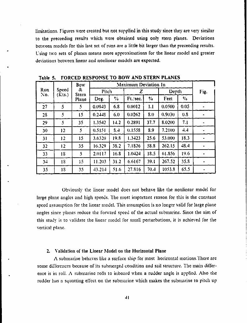
limitations, Figures were created but not supplied in this study since they arc very similar

to the preceeding results which were obtained using only stern planes. Deviations

between models for this last set of runs are a little bit larger than the preceeding results.

Using two sets of planes means more approximations for the linear model and greater

deviations between linear and nonlinear models are expected.

Table 5. FORCED RESPONSE TO BOW AND STERN PLANESBow Maximum D)eviation In

Run Speed & Pitch Z Depth Fig.No. (Kts.) Stern

Plane Deg. % Ft.,'sec. % Feet 0

27 5 5 0.0943 6.8 0.0012 1.1 0.0500 0.05

28 5 15 0.2448 6.0 0.0262 8.0 0.9030 0.8

29 5 35 1.3542 14.2 0.2891 37.7 8.0200 7.1

30 12 5 0.5151 S.4 0.1558 8.9 7.2100 4.4

31 12 15 3.63.20 19.8 1.3423 25.6 53.000 18.3

32 12 35 16.329 38.2 7.1826 58.8 262.15 48.4

33 is 5 2,0117 16.8 1.0424 18.5 61.856 19.6

34 Is 15 11.203 31.2 6,6167 39.1 267.52 35.8

35 is 35 43.214 51.6 27.816 70.4 1053.8 65.5 -

Obviously the linear model does not behave like the nonlinear model for

large plane angles and high speeds. The most important reason lor this is the constant

speed assumption for the linear model. This assumption is no longer valid for large plane

angles since planes reduce the forward speed of the actual submarinc. Since the aim of

this study is to validate the linear modcl for small perturbations, it is achieved for the

vcrtical plane.

2. Validation of the Linear Model on the Horizontal Plane

A submarine behaves like a surface ship for most horizontal 1notions.There are

some dif"'erences because of its submerged condition and sail structure. The main differ-

ence is in roll. A submarine rolls to inboard when a rudder angle is applied. Also the

rudder has a squatting efli.ct on the submarine which makes the submarine to pitch up

41

and dive. Since the linear model assumes that there is no cross-coupling between vertical

and horizontal motion it is not possible to compare the squatting eI'ect with the linear

model.

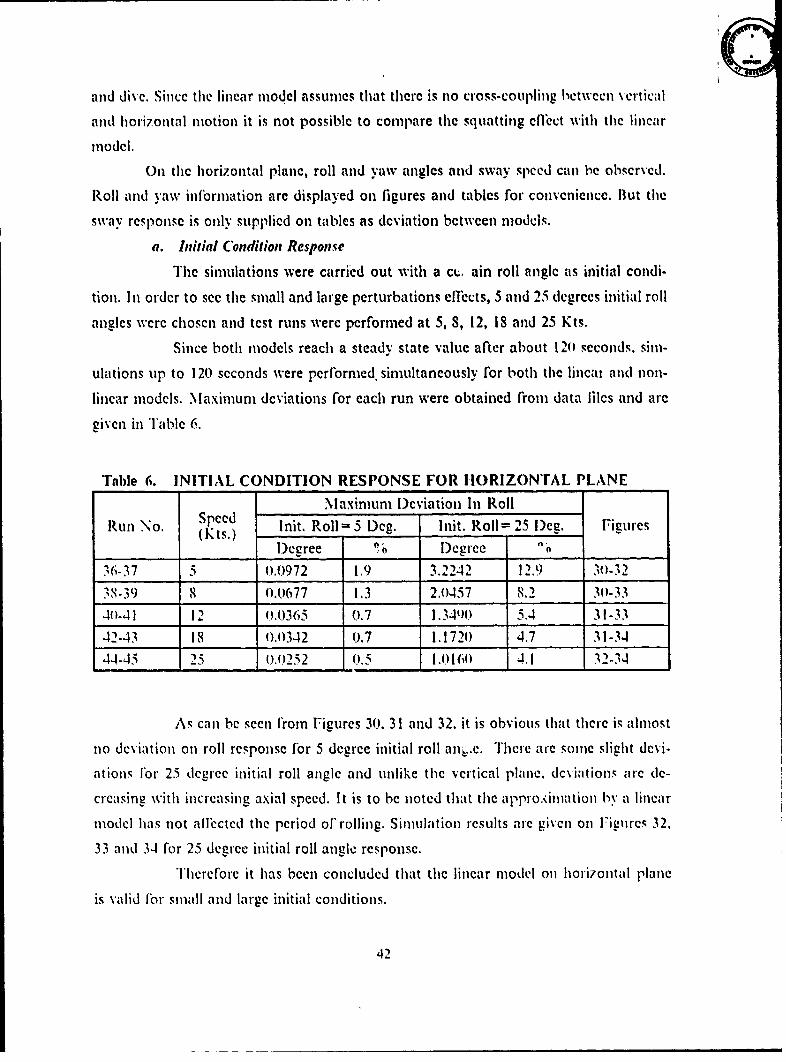
On thc horizontal plane, roll and yaw angles and sway spced can be observed.

Roll and yaw information are displayed on figures and tables for convcnience. But thesway response is only supplied on tables as deviation between models.

a. Initial Condition Response

The simulations were carried out with a ct. ain roll angle as initial condi-

tion. In order to see the small and large perturbations effects, 5 and 25 degrees initial roll

angles were chosen and test runs were performed at 5, 8, 12, 18 and 25 Kts.

Since both models reach a steady state value after about 120 seconds, sim-

ulations up to 120 seconds were performed, simultaneously for both the lincai and non-

linear models. Maximum deviations for each run were obtained from data liles and are

given in Table 6.

Table 6. INITIAL CONDITION RESPONSE FOR HORIZONTAL PLANE

Maximum l)eviation In Roll

Run No. Speed init. Roll=-5 Deg. Init. Roll= 25 l)eg. Fiuress Degree Degree ",,0

36-37 5 0.0972 1.9 3.21242 12.9 ,0-.2

38-.3 8 0.0677 1.3 2.0-157 8.2 30-33

40-41 12 0.0365 0.7 1.34910 5.4 31-33

42-43 18 0.0342 0.7 1.1720 4.7 31-34

44-45 25 0.0252 0.5 1.0160 4.1 32-34

As can be seen from Figures 30. 31 and 32, it is obvious that there is almost

no deviation on roll response for 5 degree initial roll anx..e. There are some slight devi-

ations For 25 degree initial roll angle and unlike the vertical plane. deviations are de-

creasing with increasing axial speed. It is to be noted that the appro.dmation by a linear

model has not alfected the period of rolling. Simulation results are given on IFigureq 32,

33 and 34 for 25 degree initial roll angle response.

Theref'ore it has been concluded that the linear model on horizontal plane

is valid fbr small and large initial conditions.

42

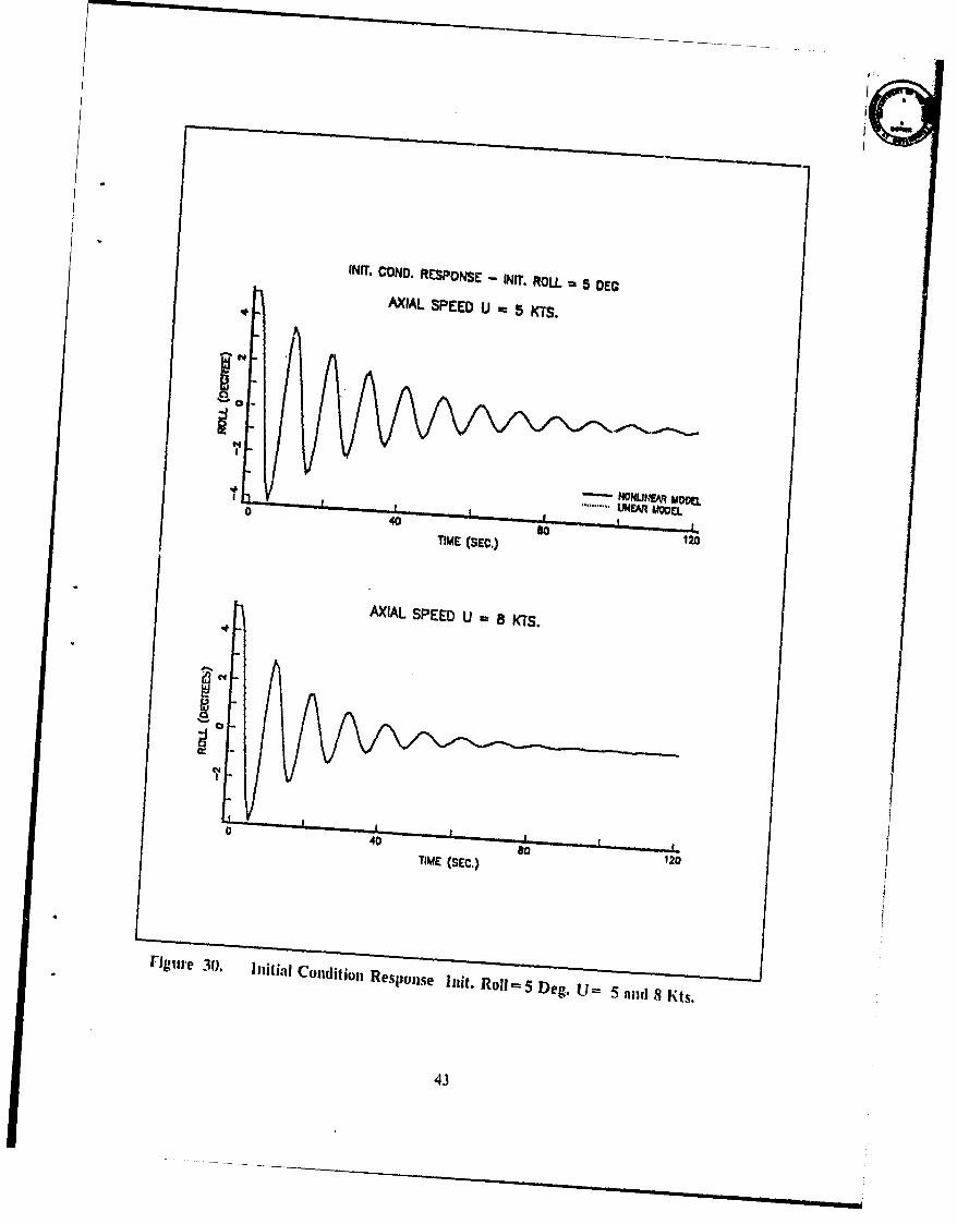
INIT. COND. RESPONSE - INIT. ROLL = 5 DECAXIAL SPEED U 5 KTS.

"0 "

TIME (SEC.) 120

AXIAL SPEED U . fI<TS.

40 TIME (SEC.) 120

Figure 30. 11ji~til Condition1 Response .it Roll= 5 Deg. U 5 and 8 Kts.,

43

INIT. CONO. RESPONSE - INIT. ROLL - 5 DEG

AXIAL SPEED U " 12 KTS.

g - I'ItILIUEAR VODELO........... IEN. MODEL

0 40 80 120

TIME (SEC.)

AXIAL SPEED U m 18 KTS.

040 so 120TIME (SEC.)

Figure 3 1. 1Initial Conditionl Responlse hlit. Roll= fi Deg. UJ 12 andl 13 IKs.

44

INIT. COND. RESPONSE - INIT. ROLL - 5 DEG


0,

- NONUEPrJ MaDE............ •IE M ,ooDE

O 40 go 120

TIME (SEC.)

INIT. COND. RESPONSE - INIT. ROLL - 25 DEG


aV

0 40 so 120

TIME (SEC.)

Figure 32. 1hnit. Cond. Response hilt. Roll= 5 and 25 Deg. U =25 and 5 lits.

45

INIT. COND. RESPONSE - INIT. ROLL 25 DECAXIAL SPEED U a8 KTS.

40 TME (SEC.) so120

AXIAL SPEED U 12 KTS.

0 4

TIME (SEC.) 120

Figure 33. Ini1till Conitiont Response fult. RolJ-25 Deg. U= 8 and 12 K~ts.

46

INIT. COND. RESPONSE - INIT. ROLL - 25 DEC


go

- MAILM4A1t MOOS.I ........... UNEmU WaDEL

0 40 80 120TIME (SEC.)

AXIAL SPEED U - 25 KTS.g

o 40 s0 120

TIME (SEC.)

Figure 34. Initial Condition Response Init. Roll= 25 Deg. U= IS and 25 Kts.

47

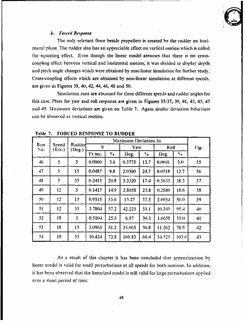
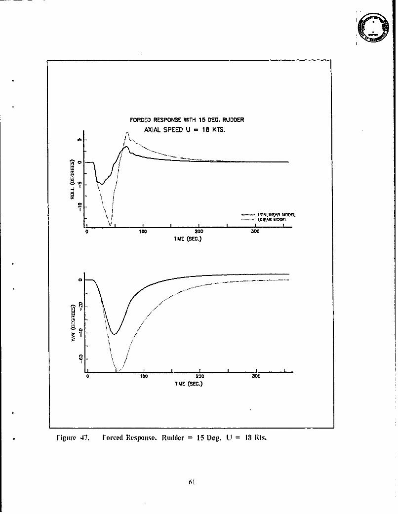
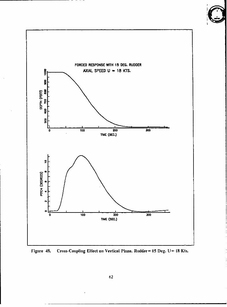
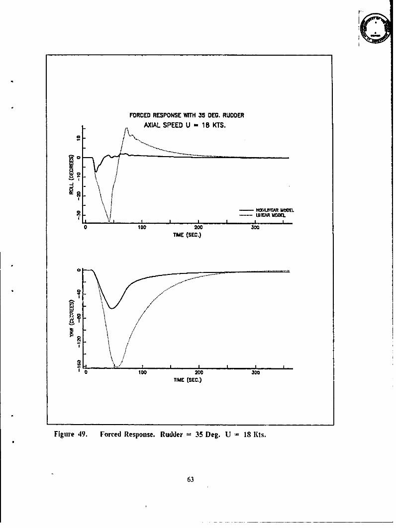
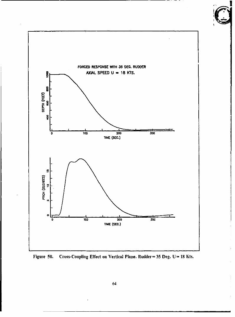
b. Forced Response

Thc only relevant force beside propellers is created by the rudder on hori-

zontal plane. The rudder also has an appreciable effect on vertical motion which is called

the squatting cifect. Even though the linear model assumes that therc is no cross-

coupling effe'ct between vertical and horizontal motion, it was decided to display depth

and pitch angle changes which were obtained by non-linear simulation for further study.

Cross-coupling efects which are obtained by non-lincar simulation at dilIerent speeds.

are given in Figures 38, 40, 42, 44, 46, 48 and 50.

Simulation runs are abtained for three difercnt speeds and rudder angles for

this case. Plots for yaw and roll response are given in Figures 35-37, 39, 41, 43, 45, 47

and 49. Maximum deviations are given on Table 7. Again similar deviation behaviors

can be observed as vertical motion.

"Table 7. FORCED RESPONSE TO RUDDER

Maximum D)eviation InRun Speed Ruddei V Yaw Roll Fig.'No. (Kts.) (l)eg.) V aRolFg

o)Ft0'sec. % l)eg. e I)cg. %

46 5 5 0.0060 3.6 0.3775 13.7 0.0041 3.0 35

47 5 15 0.0487 9.8 2.0360 24.7 0.0518 12.7 36

48 5 35 0.2413 20.8 3.3520 17.4 0. 3633 38.3 37

49 12 5 0.1417 14.9 2.8058 23.8 0.2880 18.6 38

50 12 15 0.9515 33.6 13.27 37.5 2.6034 56.0 39

5i 12 35 3.7804 57.2 42.223 51.1 10.345 95.4 40

52 is 5 0.5104 25.3 6.97 30.3 1.6658 35.0 41

53 18 15 3.0963 51.2 35.065 50.8 11.262 78.9 42

54 IS 35 10.424 73.8 106.83 66.4 34.525 103.6 43

As a result of this chapter it has been concluded that approximation by

linear model is valid for small perturbations at all speeds for both motions. In addition.

it has been observed that the linearizcd model is still valid for large perturbations applied

over a short period of time.

48

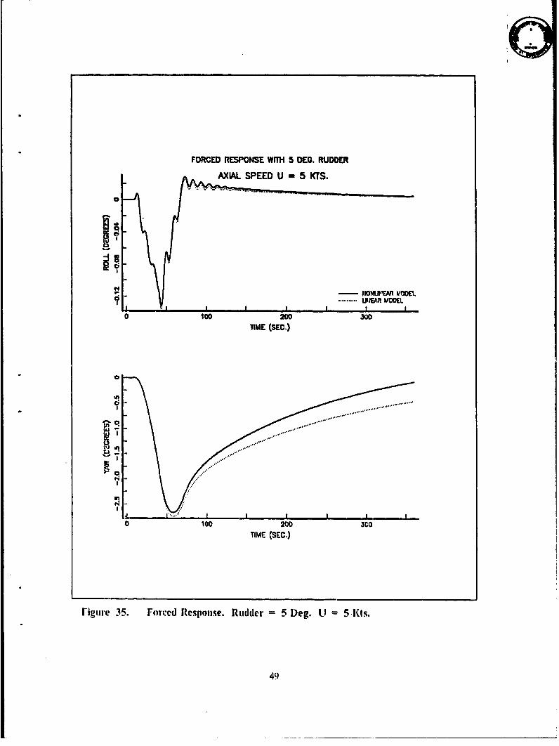
FORCED RESPONSE WITH 5 DEG. RUDDER


s

- I0ONUI'T.J1 M'OOEL

I ,........... UE MO EL

0 100 200 300TIME (SEC.)

So°o................. ....... ............. .....

0 10O0 200 3:00

TIME (SEC.)

I'igurle 35. Forced Responlse. Rudder = 5 Deg. IJ 5 SKis.

49

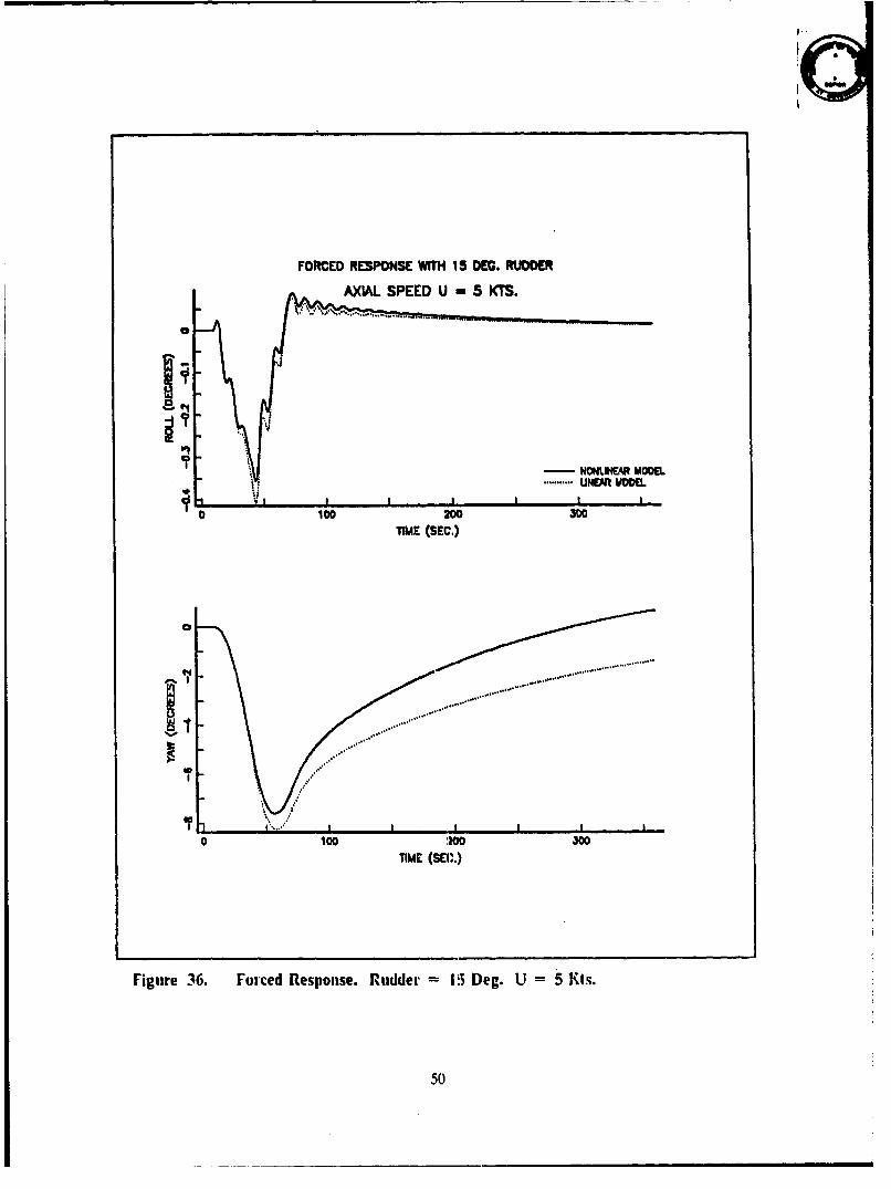
FORCED RESPONSE WIH 15 DEQ. RUDDER

-NONLII-AR MOMI

....... UNEAR MOOB

0 100 200 300TIME (SEC.)

a ..................... ..... .................

0 100 TIME (SEC..)

Figure 36. Forced Response. Rudder 1 I5 Deg. U =5 Kits.

50

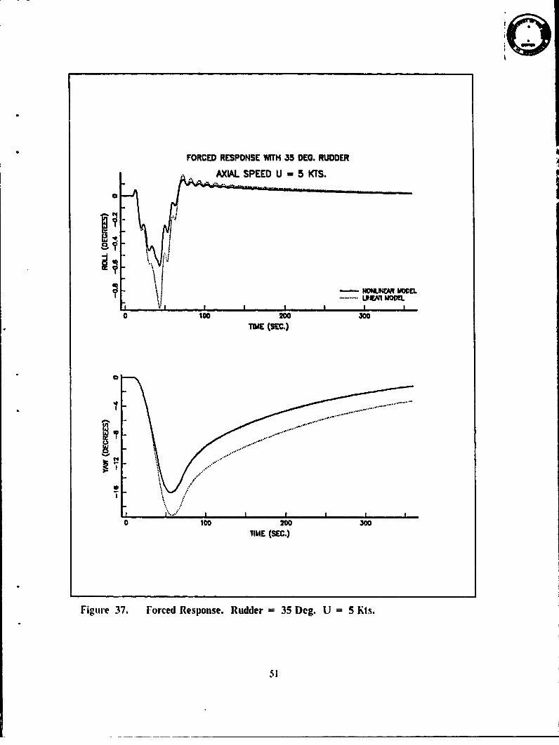
FORCED RESPONSE WiTH 35 DEC. RUDDER

AXIAL SPEED U- 5 KTS.

C3'.

........... lR mo EI.'I I WJ! OV!

0 100 200 300TIME (SEC.)

". .... ...........IrT " I..* /

o 100 200 300TIME (SEC.)

Figure 37. Forced Response. Rudder = 35 Deg. U = 5 Kis.

FORCED RESPONSE WITH 35 DEC. RUDDER


x

o o00 200 300TIME (SEC.)

i'1

0 100 2o0 300TIME (SEC.)

Figure 33. Cross-Cottpling Effect on Vertical Plane. Rudder= 35 Deg. U = 5 Mts.

52



B.

- NONUNDCAJ MODEL........ URE.At MODEL

0 100 2C0 300TIME (SEC.)

p 0,, .. ............. ...., ............. ...

.. ... ..... ... ... . .... ,........ ........ .

..

LUL

I0 100 200 30

TIME (SEC.)

rigure 39. Forced Response. Rudder = 5 Deg. ILI = 12 Ets.



.4

0 100 200 300TIME (SEC.)

U

d-.

0 100 200 300TIME (SEC.)

rigure 40. Cross-Coupling Effect on Vertical Plane. Rudder= 5 Deg. U 12 Kts.

54

FORCED RESPONSE WfTH 15 DEG. RUDDER


a

S................ UEPR MDEL

V II I ' I I

o 100 200 300

TIME (SEC.)

.. . .. ... . .. ... . .. . .. .......... .......... ..............

..... .......................

Is-,

01 O0 200 300

TIME (SEC.)

rigure 4 1. Forced Response. Rudder =15 Deg. doisn. Ll 12 Kils.

55



0 100 200 300

TIME (SEC.)

0 '1O0 200 300TIME (SEC.)

Figure 42. Cross-Coupling Effect on Vertical Plane. Rudder= 15 Deg. L = 12 Kts.

56


AXIAL SPEED U -12 KTS.

- NONUNEAR MCCCL.....................................................U14r.AR MCCCL

I I p

o ¶00 200 300liME (SEC.)

a

'C

I I I

0 100 200 300



0 100 200 300TIME (SEC.)

a

0 100 200 3•00

TIME (SEC.)

Figure 44. Cross-Coupling Effect on Vertical Plane. Rudder = 35 Deg. U 12 Kts.

58

FORCED RESPONSE WITH 5 DEG, RUDDER


-]0NLoNtEtR MODEL........... UIER MODELr . 1I , I I I I

0 100 200 J0GTIME (SEC.)

.. .. ... .. ....... °.. -. . ..................... ............................................

SI ,

0 100 200 300TIME (SEC.)

rigture 45. rorced Response. Rudder 5 Deg. U = 18 Kts.



0 100 200 -OOTIME (SEC.)

eLi

0 100 200 300TIME (SEC.)

Figure 46. Cross-Coupling Elfect on Vertical Plane. Rudder= 5 Deg. U= 18 Mts.

60

0


AXIAL SPEED U = 18 KTS.in

,. .. ... .....

ld S•~ ?D0M.NLi'FJR MOV',ELa.......................... ..............

" .. " ........... UNIEAR M,.'ODEL"p II II

0 100 200 300TIME (SEC.)

0 ,-• S....... .................... ..... .................. .. , ..... ...........................

.....

0

'I',

..... .. ........ .. i

0 10D 200 300

T!UE (SEC.)

rigure 47. Forced RIesp)onse. R'udder = 15 Deg. LU 13 i•ts.

61

I


AXIAL SPEED U 18 KTS.

P

"In

0 100 200 300

TIME (SEC.)

a

g-

Li

0 100 200 300

TIME (SEC.)

Figure 48. Cross-Coupling Effect on Vertical Plane. Rudder= 15 Deg. L= 18 lts.

62



'-I\

0

""I *-...UZM 100

..........u.. ........

IIII I II

100 200 300

TIME (SEC.)

• ,."/

.........

"" 100 200 300

TIME (SEC.)

Figure 49. Forced Response. Rudder = 35 Deg. U 18 Kts.

63

I

FORCED RESPONSE WITH 35 DEG. RUDDER* AXIAL SPEED U ,18 KTS.

I

0 100 200 3JOTIME (SEC.)

0 100 200 30CTIME (SEC.)

Figure 50. Cross-Coupling Effect on Vertical Plane. Rudder= 35 Deg. U- 18 Kts.

64

b4

/dk h

dS c~ 1/5/ Pitch

Figure 5 1. Signal Flowv Graph for Vertical Equations of Motion

d = - 6. 67x 10-4 11

e= 3.19.v10 `W

1*= -;. 36A I i)it

g I .SSA10 5 ul -2.52x1& 3-

It = O706it

i 0.013 - 1.73x1O-zi'u

k= I.SSxl10-51

1. Decoupling

In ordcr to design a cascade compensator wvith a single loop techlnique, one must

have the independent input-output relations for each input and output I1kef. 7 1. In

other words it is necessary to obtain two transrler functions for depth and two transrer

functions for pitch which have the stern aid bow planes as inputs.

Applying M-ason's gain rule to the signal flow graph given in Fig.44 the input-

output relations wvill be as follows [Ref. 8: p. 831.

66

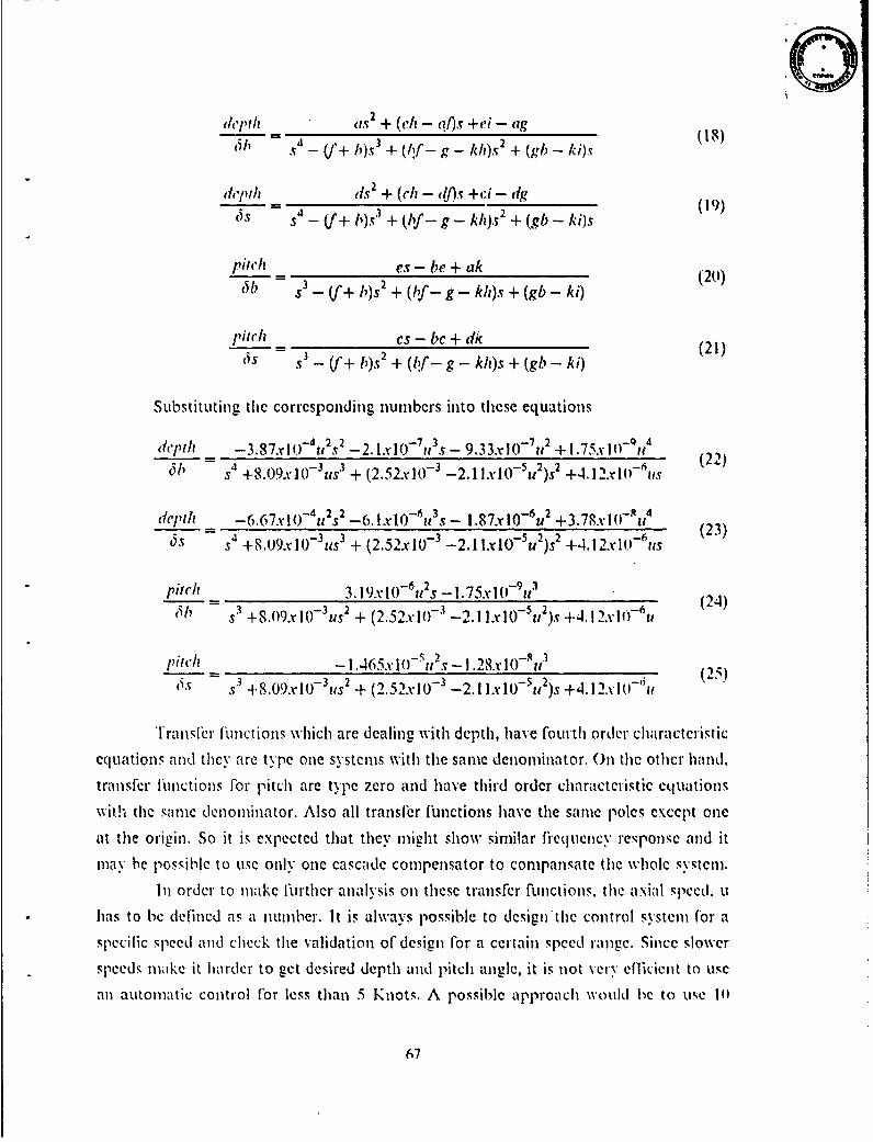
depth as 2 + (ch - aI)s +ei - ag

S- - s _ (f+ b)s 3 + (If- g - kh)s 2 + (gb - ki)x (18)

depth ds2 + (4lh - JU)s +ci - dg(is s' - (f+ 11)s' + (1f- g - khl)s 2 + (gb - ki)s

'itch 2 es - be + ak (20)6 b s3 - (f+ b)s2 + (If- g - kh)s + (gb - ki)

I'itch cs - bc + dk

j)s s' - (f+ b)s2 + (!f - g - kh)s + (gb - ki) (21)

Substituting the corresponding numbers into these equations

dlepth - 3.87xlIt)-4 2s2 -2. lX10- 1(3S _ 9.33x10- 7u 2 + 1.75.v 1- -Q14S31 322 -6 (2s4 +8.09l0-USl + (2.52x.10- -2.11.10-u2)s +4.1 2.1l) us

dcth' -6.67x1()-42 S -6. 1x10-6 i 3s - 1.87x10-6u2 +3.78xl -"4 (23)Os s4 +8.0)9X.i0-3us 3 + (2.52x10- 3 -2.1 lxIO- 5 u 2)s2 +4,i.2x.lO 6 us

pitch 3. 19xlO 6it 2s -u !.75x ! (2)t4

s3 +8.09X 10-3 us 2 + (2.52x 10-' -2. 11 x l0-Su 2)s +412.57us

1'itch - 1 .465x1(' 5 u2s - I .28x 10-i15(s s.3 4.S.09x10- 3us 2 + (2.52x10F3 - 2.1 lxlf-5 u2)s +4.l.12.v.I' -'it

Transficr f'unctions which are dealing with depth, have fourth order characteristic

equations and they are type one systems with the same denominiator. On the other hand.

transfer functions For pitch are type zero and have third order characteristic equations

with the same denominator. Also all transfier Functions have the same poles cxcept one

at the origin. So it is expected that they might show similar Frequency response and it

may be possible to use only one cascade compensator to compansate the whole system.

In order to make further analysis on these transfer functions, the axial speed. 1u

has to be defined as a number. It is always possible to design the control system for a

spCcilic speed and check the validation of design for a certain speed range. Since slower

speeds make it harder to get desired depth and pitch angle, it is not very ellicient to use

an automatic control For less than 5 Knots. A possible approach would be to use 11)

67

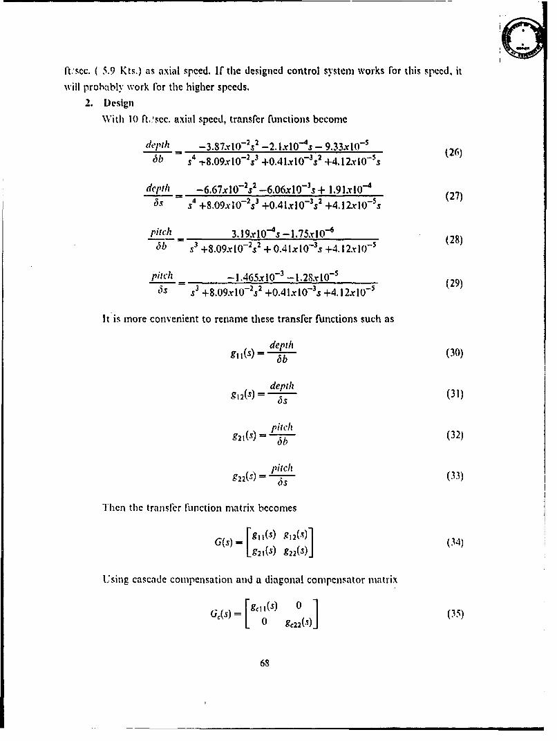
ftvsec. ( 5.9 Kts.) as axial speed. If the designed control system works ror this spced, it

will probably work For the higher speeds.

2. DesignWith 10 ft.'scc. axial speed, transfcr functions become

depth _ -3.87xi0- -2. lxIO4s - 9.33x10-S6b S4 3-t8.09x10-2s3 +0.41xIO-3s2 +4.12xl0-fs

depth -6.67x1 0-2s2 -6.06xlO-s + 1.91x10-'Ss - S4 +8.09x1O-2s3 +0.41x10-3s2 +4.12xl0-ss (27)

pitch 3.19xIO-4s -1.75x104 (28)

bb s3 +8.09xlO-2s 2 +0.41xl0-3s +4.12xl-0 5-2

pitch - 1.465x10- 3 -1.28x10- (29)

6 S -s3 +8.09xlO- 2s 2 +0.41xIO-3 S +4.12x.lOf

It is more convenient to rename these transfer functions such as

depth (30)

bb

g92(s) dept (31)5S

g21(s) = peih (32)

g2 2(S) /I ptch (33)OS

Then the transfer function matrix becomes

G 9)= 11(S) 912('S) (4g921(s) g22(s).l

Using cascade compensation and a diagonal compensator matrix

Ge(s) = I O(S) (35)0 g,220.) J

68

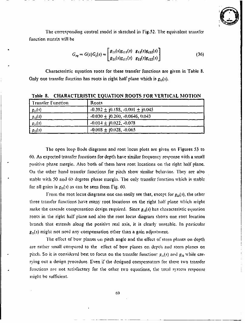
T*he corresponding control model is sketched in Fig.52. Thc equivalent tranisfer

function matrix will be

Lg2i(s)gC11(s) g22(s)g22(s)J

Characteristic equation roots for these transfer functions are given in Table 8.

Only one transfer function has roots in right half plane which is g1 (s).

Table 8. CHARACTERISTIC EQUATION ROOTS FOR VERTICAL MOTION

Transfer Function Rootsg,,(s) -0.392- ± j0.188, -0.001 + j0.045

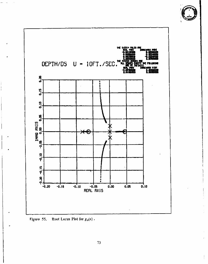
g12(s) -0.030 ± jO.260, -0.0646, 0.043

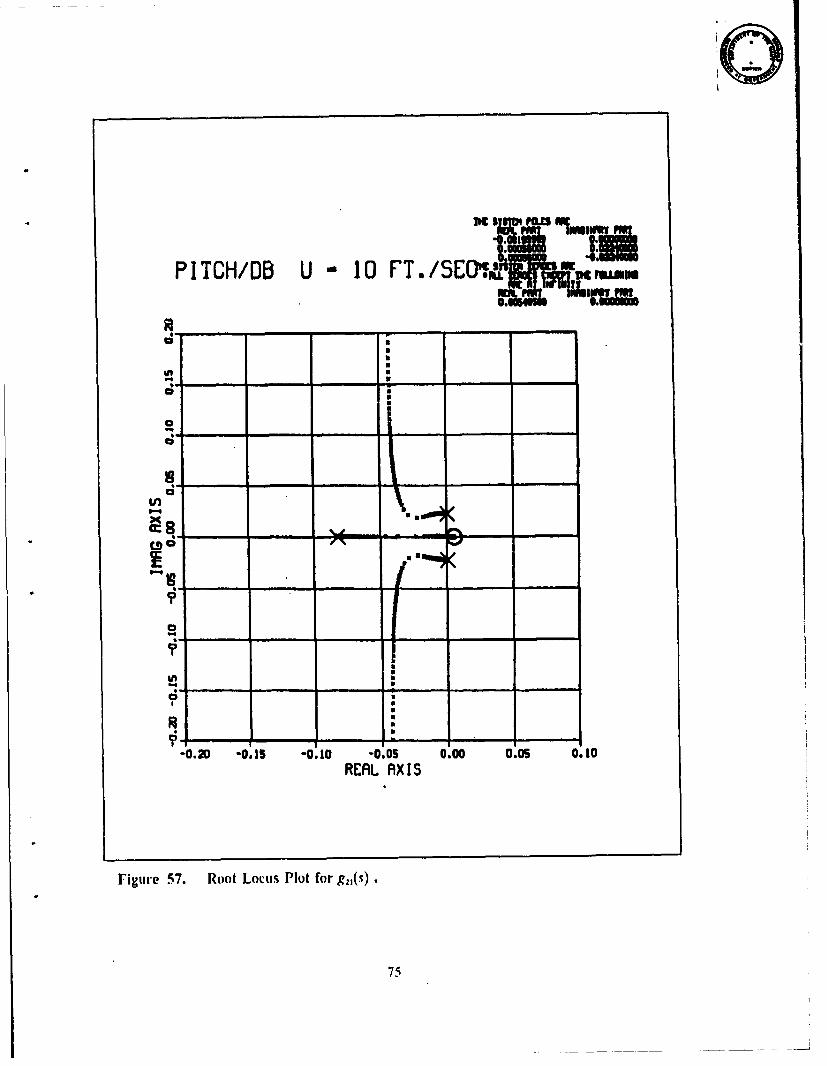
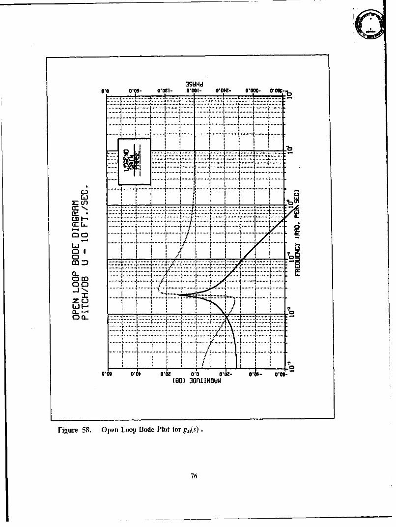
g-,(s) -0.014 ± jO.022, -0.078

gh2(s) -0.008 ± j0.028, -0.065

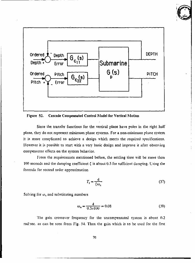
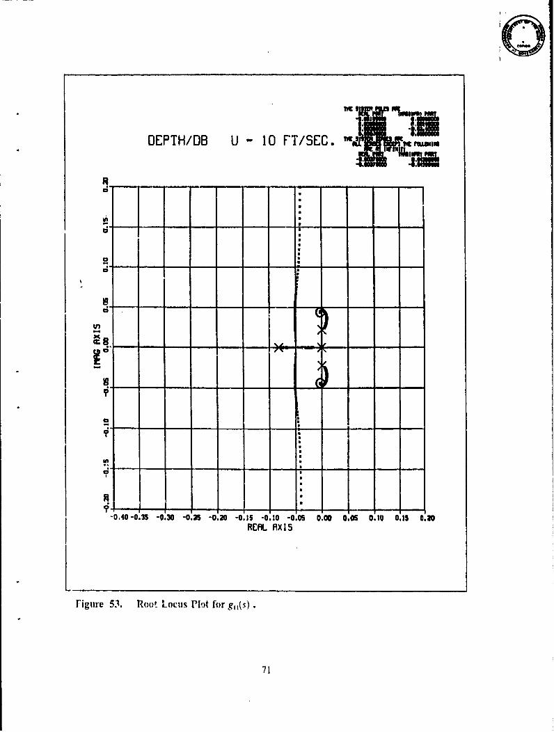
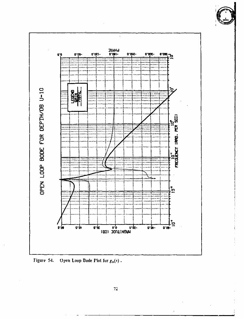
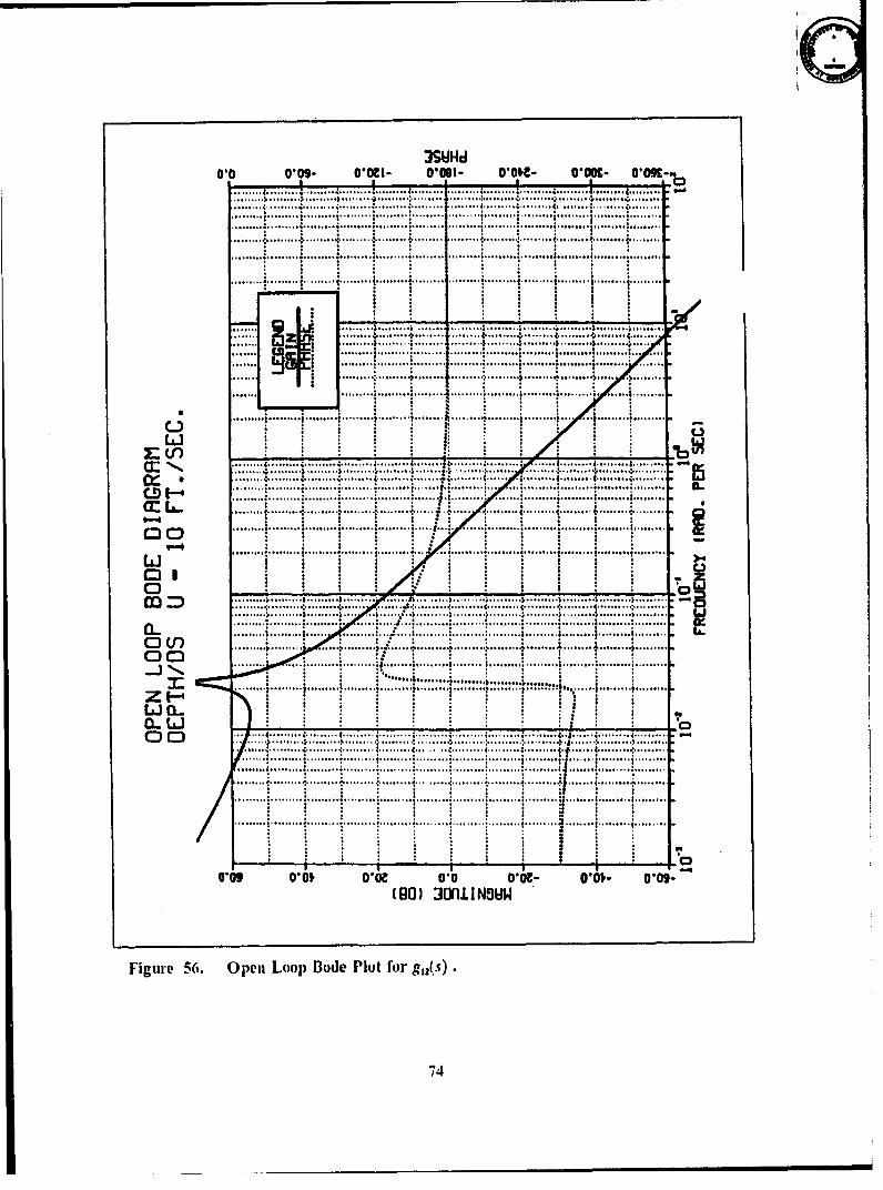
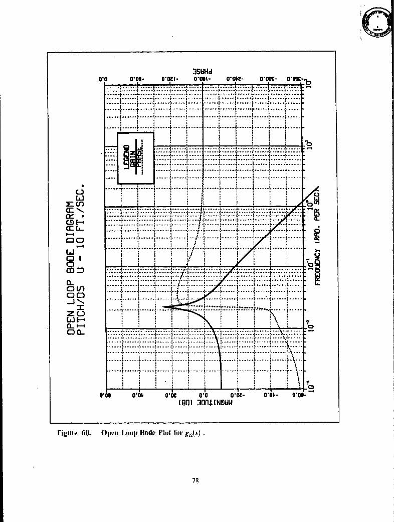
The open loop Bode diagrams and root locus plots are given on Figures 53 to

60. As expected transfer functions for depth have similar frequency response with a small

positive phase margin. Also both of them have root locations on the right half plane.

On the other hand transfer functions for pitch show similar behavior. They arc also

stable with 50 and 60 degrees phase margin. The only transfler function which is stable

for all gains is g, 2(s) as can be seen from Fig. 60.

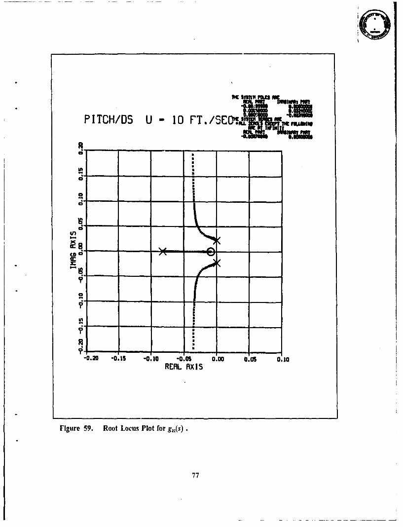
From the root locus diagrams one can easily see that, except for g2 (20), the other

three transfer functions have many root locations on the right half plane which might

make the cascade compensation design required. Since g12(s) has characteristic equation

roots in the right half plane and also the root locus diagram shows one root location

branch that extends along the positive real axis, it is clearly unstable. In particular

g:,(s) might not need any compensation other than a gain adjustment.

The effect of bow planes un pitch angle and the effect of stern planes on depth

are rather small compared to the cillect of bow planes on depth and stern planes on

pitch. So it is considered best to focus on the transfer functionw g,,(s) anld g22 while car-

rying out a design procedure. Even if the designed compensators for these two transfer

functions are not satisfactory for the other two equations, the total system response

might be sufficient.

69

"Si.

Ordered Depth 6e(S) DEPTH

Depth + Error Submarine

Ordered Pitch 6 (S) PITCH

Pitch + Error C22

Figure 52. Cascade Compensated Control Model for Vertical Motion

Since the transfer functions for the vertical plane have poles in the right half

plane, they do not represent minimum phase systems. For a non-minimum phase system

it is more complicated to achieve a design which mects the required specifications.

H lowever it is possible to start with a very basic design and improve it aFtcr observing

compensator eflects on the system behavior.

From the requirements mentioned before, the settling time will be more than

100 seconds and the damping coefficient C is about 0.5 for sufficient damping. Using the

formula for second order approximation

TS = 4 (37)

Solving for ),, and substituting numbers

4 .5xlO0 =0.08 (38)

The gain crossover frequency for the uncompensated system is about 0.2

rad'scc. as can be seen from Fig. 54. Then the gain which is to be used for the first

70

00

I S '

- Io)q' I

ri r 53 o ! L o u l tf r ,( .

71

010 0109 01091 0*091 0*08- aSC- 0

............................... ..... .................. 4.................. 4.....

. .. ....... .............. .........4 ...... 4....

.........

.4................ .....

.. ... ... . . ........ ... ..

, ..... ........ .... .... . ......... .LL....................... ................ 4... .. ................

...... ...................2..... .... .. . . . . . . ......

0~... ... .. ... .......

0 .......... ,

.... ...... 1 -t .... ............ ..........

I /....... ................9

..........

.4

...... ft .. ..

~... ................................... 1... .2.. `.. ... ..I.. .. .. ... ... .. .. .. ... ... .. .... .... . ....

......I...... ................... I. .................

... ... ... ... .. 2 .. .. . I . .. ... ....... I .. ... ... ..... . .. .. ....

(90) 3anitNUWW

Figure 54. Openi Loop Bode Plot for g,,(s).

7 2

tot I P3.5 Ug

OCPTH/O5 U I OFT./SEC." 'u

tnU

a %

- UE

o 4o-02 _01 01 OO 0 .s 01

RELAXI

ritv 5 otLau ltfrgs

ij~a _ 4'

JSUNHd00 0109- o0"e1- o01u1- 0109i- 0oo0t- OO -

.4 ....... ............... ! .... ... ................... ! ....... . .. ..... .. ab ........b 4 .................."... ......'" ....... .. .. ",.,.. ... .... .......... ......... ..... .... ............................ ................... .........

S ................... .... ..................................... .. .S... ... ......... i......... •......... ......... ......... ......... ......... .......... ......... ......... ! ... . .S........ !.........". ........... ......... t ......... ? ......... ......... ......... !..........I ......... t.........t........ .S......... -......... •......... :.......... : ......... I ......... .......... I ..... .... 'I ...... ... 'I....,..... I......... ..... ,...

S........ " ... ..... ........... ; ......... t ........ . . ..... ........ ! ......... t......... t......... !.. .' ..........

. . . . : . ... .

S....... P I e I ........ 4......... .. ......... i. ......... , ......... 4.........., ......... 4,........ . ... ..... w.. ...... .......... .. ................... ...... ......... .........

,,.,........... . ....................... ..... I..... ....... ..........'....... ......... *......... '........ :1......... .......... , ......... :......... ....... ......a- ..

"CC N%. .... ........... ... . I"'. . . . . . .. --. .. .

* 2r-~ ...... .......... .........

rmn .

S... ...•......... )......... •......... ,........ •..... .... • ........ ...... : ' .. ...... .......... .......... ... .. ..

.. . ., , .,; ... ,................ .... ;....... • ...... : ........... ........ ....... ...... ,.... ............ ........ .

cr ...... • ..... ......... ......... .......... •...... ' ..... . ....... f ........ • ......... ,......... 1 ......... .

. ..... ".'........ '"'.... I' " ...0-4

S......... .......... ............ ..... . .... . .... 4.. '....... €............ ......... •..'....;.. ......... .

0IS.. .. ... .......... .. ........... . ....... ......... ......... ......... .........

M =. I. ......... .... ; .. . . . .. . . . .. . . .

•QC ) O• ..... ~ ~.... : ......... :......... ' .. .." ' '" ......... "....... :......... :......... ......... ......... . .........S..... .... i.. ... ...... .. ... . . . .o ~~~ ~ ...... . .... ....... ............... ..... ................ ........ .......... .........o... ............................ .... ...........

LiNC

"00,.. . .......................... ..................... .......

S......... l......... i......... i........... ......... ......... ......... •. . ... .- .:. ' .. .... • ....... .. i....... .

b.1 Q. / ! : : : : • . .

"............... "' ................ ....... . ........../...... •......I.,.. •......... •.......... ........... ......... . . ... . ......... •......... €. ...... €..........•. .........r -. ............ i......... ......... ........ ......... . ......... i......... . ......... , i......... ......... .

01o9 010I lot OO 0orW ra0- 0ag-,(GO) J3flLNOUW1

Figure 56. 0Opent Loop Bode Plot for g,,ts).

74

fie SIM, mn NPl |lM 11palwl m-

PITCH/DB U 10 FT./SEQ.DI , g I ,l

fm T

Ii

-0.2- -. 1 -0..- -0s -.0 OOs 01

o a

575

-020 -0. -01 -OO -.0 -.' ,IRELa

Fiure, . Ro ou Po o 2(,)

p.45

JSUI4J0.0 n*0- roil- ro00- ro011- r10ot- 01c

........... 4 ...... .... ....... . ....... I...........4 . .................. . . .. . .

........ .... .... ..... . . . .4 . ........... . ~ 4

9 z ...... .... ....

... 4. .....

4..... 1 ....... 4.......b

UC.... .... ........ ....).......... I ...... .

LD .a.............. . . .. .....

.4 L ....... I........ ..... ....4 . 4... ...'F' ......I. .4..

U o ..... .

0.... .....i

Q~I-I

I~ I0*U ...... ...... 00 . t 0 5 0TGO ......II.....

ri ur ..... O...... Ltj ....de. Plo ..or.....)

...... ..... ...... ...... ...76.

0

SfiePITCH/OS U - 10 FT./SCO¶'~ 3 ofTl UNI

Uq -,

a U

-s

0C. -_n-

aN

! ...... .. .. ..

-0.20 -0.15 -0.10 -0.05 0.00 0.0 0.10

RERL nx IS

Figure 59. Root Loculs Plot for g,,(s)•

77

3SNcd0'0 000S- WWI- O'OI- 01OOt 0010- O0OC-b

..... ...... ..... ......... .. . ................ .... :*. ......... ...... 4.... .. .,.. ...... .. ....... ., ......... -........ .:....... ........... ......... , ......... ......... .......... .........

.. . ............ ' ** *' *" * * ......... t......... . .................. * ................ ............ , ** ......... ,'........ .S....... ........ • .. .... .: ......... "........., ......... ......... I ..... ....I ......... [......... ......... ......... .

........................S........ •........ ÷ ........ .. ........... ......... ......... .......... ......... i..........i ......... i......... •..........S.... .... .................. , ......... ......... .... .......... ......... , ......... , ......... ........... .. .. ............. . ................. ...... ......

- ......... . ........ .. .. .. ......... ......... ......... ......... ......... ... ...... . . . . :.. . . 1 1. 11.. . . I ' l l '".. . . .. . . . ! . . . . . . . .. " . . . . . . . . .€ .. . . .4 . . . . . . . .. ? . . . . . . . .S.......... : ......... ).......... ....... 4.. . . . ......... ...... ,... ......... •..........S......... i......... •... I..... .......... ,.. .. .•. ....... ......... ', ......... •..........

: .......... I ......... ........ .......... ......... i......... ,. ......... % ........ .!.........S....... i .......... ,"......... ....... I. ......... ......... "•........" .......... , ......... " .........

................ i ........ .............. ......... ......... ......... ......... ..........

CC....•... .. • .... .... ......... ... ......... = ........ . .... ......... ......... • ....S. .. . .i ... . .. ... . . . . . . .i. . .. . .........I. ......... ... .. .. :.... .. . .......... i...... %% ..........o° ...;, o...... l..........: ......... .%........ l...... .. : ......... ,.................,...* ..... * *.. ... **|... ..... i......... .. ......... ".,........ ..... ... •. .... • ...' ...... .. • ......... i......... .......... .. .. .. . CF " ..... ..... ..... ..... ... .. - ....... i......... •......... ......... .....

C ......!........ ......... ......... .... .. .. .... ...... i....i • ..-. ..S........ . .... .....

......... •........... •.. ......... ... . .......... .... .•......... . ..., ........ .... .. ... ......... •........ .

C3 0

............ ...................

..... ......... .....

m ..... ..... .. ......... . ........ ........... ... . ......... ......... .............. 1 .... ......... e :.,,,::::.a ......... ......... .. ....... ............, ..,I ............... .... .............

"Li _ _ _ - ' ''' i •

O ..... ......... .. ....... ..... ......... ,.... " ". .....

0 ........ ......... ......... . .. ....... •..... .... ....... .. ...... ..• ......... .......... ....... ., ....... .. • ........ .

. . . . . .......... . ......... ...... ..S... . ...... . ..........................

Zt L)

Li F-S

oa-.. .. .. . .. ... ... ... ... . .. ...

S......... i......... i..........•. ......... i......... !......... i..... ..... .......... 1......... . . . . . . . . . . . . . . .

""'. 4' .....

OSO . N,. NU

C......................... ..... . ..... ...... . ...

D..I ... ..... ......... .... .... ......... ......... 6 .....

09 0101 ODEt 0*0 O'Dr- 0*01- 0109-(w ) a nJilINSUW

Figure 60. Open Loop Bode Plot for g,,Is).

78

compensator. has to be less than one in order to get the desired response. This gain

constant is called K I and taken as 0.1 for the first trial.

In order to increase phase margin a first order lead compensator is to be added

to the fbrward path. Such a compensator has the form

-= (s+z) (39Sz (s + P)

The multiplier p.z is required to keep error coefficient constant. ItRef 2 1Using cascade compensator design techniques the best choice for the first trial

on gon will be

i s+. 10 (s + 0.1)

0.1 s+l.O s+1.0

Nfultiplying with K I the total compensator is

s+0.l (41)s+ 1.0

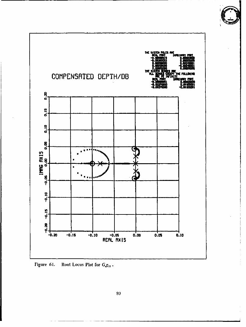
Thc root locus plot and open loop Bode diagram for the compensated system

are given on l ig.61 and Fig. 62. The compensated system has about 75 degree phase

margin which is obviously more than the specified requirements. This excess p-hase

margin may cause a request for the large plane angles which it is not possible to supply.

Since it is always possible to use limiters on plane angles it is concluded to leave the

designed compensator as it is and use it For preliminary design procedures.

Since¢_.(.) is already very reasonable well damped, no compensator will be used

and K2 will be taken as L.O For the first trial.

The next step is to put the compensator in the actual linear system and observe

the response of the system. But before doing that the simulation program has to be up-

dated in order to get more realistic results and accuracy.

a. Limiters

The mechanical linmit For both plane deflections is 35 degree. But it is not

desirable to use full plane angles for higher speeds. Also it is possible to limit planes and

the error sicnals. "rhe test runs which are achieved with limited planes led to unaccepta-

ble plane behavior such as Very small deflections. Under these set of circumstances it

was concluded to limit the error signal such as:

79

4

""tiCOMPENSAITED OEPTH/OBoi

Cin

.4

C"

I--

-0.20 -0.15 -0.10 -0.05 0.00 0.05 0.10REAL AXIS

rigure 61. Rout Locus Plot for Gig,,

so

0*0 ~ - ret- SUHJ

010 0,9- 011 cut09- rolog- root- owm-

I.......................

S...........

.................................. .....

.. .. ..%.... ... .. .........el

....... .1... . .. .. .. .. .. .. .. . .. .. .. .. . .. .. .. .. . . .. . . . . . .. . . .

0. ........ .... ... .... .... ........ .... ....

C~lb.4.... ....... ......... ..... ..... .... .

.. .. .. . ..................1 *:' ...... . 1. ..... .... ..... ..... ....

- I-... .................. I ...... ........ ............... .C 3 ~ 0 0 0......... ...... 0 ......... .. .... ....... ......- .............. -..

...... (.. ........... i...... ..... uw....

rig.............. 62.... Op, Loop.. Bode... Plot... ..or.. G................

a _ ..... ...... ..... .... ...... .... . ... ... .... .... .. ..... .... ..... ... ..I

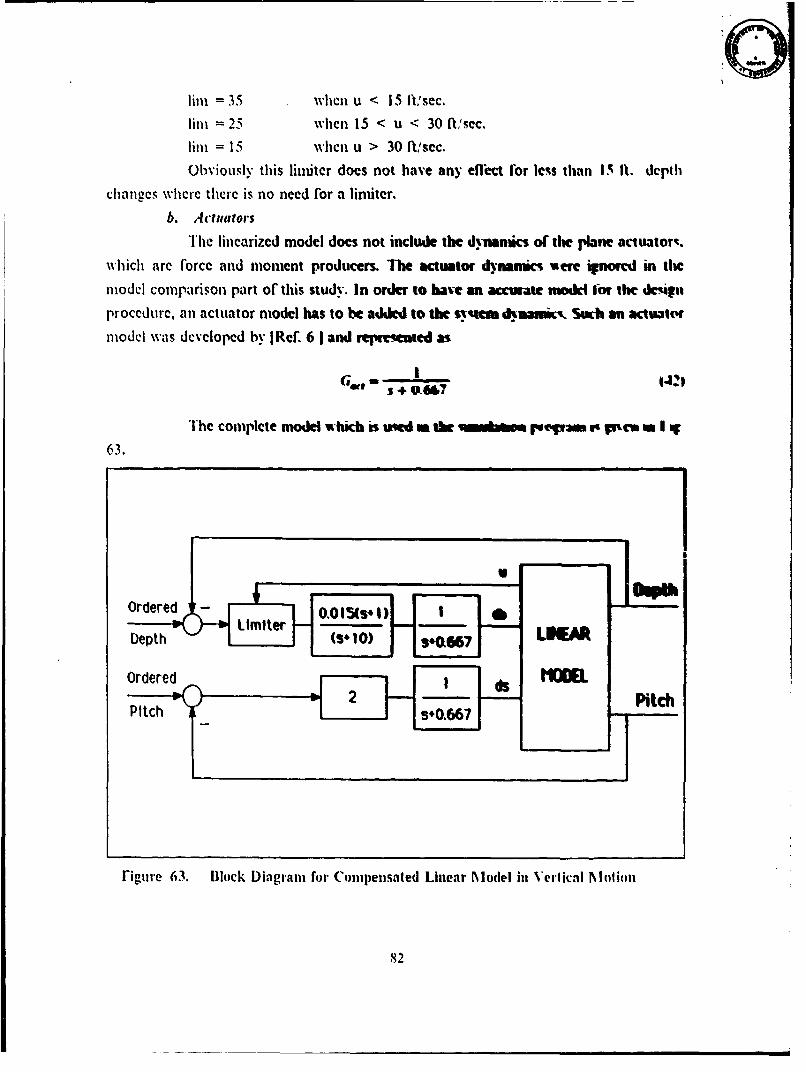
lim = 35 when u < 15 fl,'sec.

lir = 25 when 15 < u < 30 fl,'sec.

lira = 15 when u > 30 ftlscc.

Obviously this limiter does not have any effhct for le.s than I5 11. depth

chanecs where there is no need for a limiter.

b. Actuators

The linearized model does not include the dnammics of the kaune actuator%.which arc Force and moment producers. The actuator dynancis •ere ignored in the

model comparison part of this study. In order to have an accwate wedk tot the deiti

procedurc, an actuator model has to be added to the s-tem dunm'. S.oh an actuator

model was developed by IRef. 6 1 and mewesated as

The complete model which is awed a the %w I~ rv m Irt Vnep m I q

63.

Ordered " 7 LEI

Ordered, MO__OI 2 ]Pi

Pit4h Pitch66

rigu'e 63. Block Dingram for Compensated Linear Model in Vertical Nfloliot

82

3. Simulntioti

The simulation program is written based oil the discussed subjects above. The

first run was made with the preliminary design gains, poles and zeros. 1h1en required

corrections were made in order to meet the design specifications. Tlhe i)SI. simulation

program with the final parameters is given in Appendix F.

Test run results which were achieved with diffierent sets of parameters are givenin Figurcs 64 to 74. Each run is explained briefly below:

Run No. i:

"The simulation program was run with the first set of parameters for 10 11. depth

change and 10 ft;sec. axial speed which is the lower limit for this compensation. With

K I =-0.1 the required bow plane angle was very large and overshoot was 25%. This run

does not meet the specified requirements.

Run No. 2:

In order to get reasonable plane response it is decided to reduce K I to the value

of 0.91. This time the maximum bow plane deflection is 26 degree but the timc required

to reach 10 flet depth change is a little longer than the specification. This run is also

discarded.

Run No. 3:

A third approach would be to change KI to 0.015. The result was quite satis-

factory except the 40 degree maximuIm bow plane angle. The main reason for this larger

plane request is the excess phase margin on the system. The one possible way to reduce

phase margin is to shift the cascade compensator one decade up in the frequency do-

Imainl.

Run No. 4:

Using the new compensator with one zero at 1.0 and one pole at 10.0. the results

are satislhctory. As can be seen from figure 66 the maximum required bow plane angle

is 10 degrees, the time to complete 10 ft. depth change is 78 sec. and the overshoot is

106. This excess overshoot is the payoff for reducing the phase margin but since it

makes only one fbot dilkierence, it is acceptable.

Run No. 5:

It is desired to check the system response for large depth chalnges. The simu-

lation program was run For a 100 ft. depth change. Maxinium required bow plane angle

83

is 34 degrees and overshoot is 5%. At this point it seems that the compensated linearmodel (or Cdepth control is acceptable.

It is also required to check the pitch response of the system. Test runs wereperflormed with zero depth and some certain pitch angle change. Because of' the bowplane efl'cct (which tries to keep the submarine at the same depth) there was a stead'state error on pitch angle. Since this pitch error relates very closely to K2, it is concluded

to increase K2 to 2.0.

Runs No.6 and 7:

"1"o make sure that there is no negative effect on depth behavior of the systemcreated by the hew K2 parameter, two more runs were achieved with K2= 2.0 I'or 10 and

100 lizet depth change. Since there was only a slight change on overshoot, the new K2value is accepted and used for further study.

Run No. 8

In order to check the pitch response of the compensated system, a .5 degreepitch command was ordered while the depth change command was zero. Syrtcrn hasreached the ordered pitch angle in 46 seconds and because of" the bow plane eflect, itsettled on -4 degree. Increasing K2 might decrease this steady state error but at the sametime it might create more overshoot and instability problems on depth behavior of thesystem. Since a I degree error is in the specifications linits, K2 = 2.0 will be used for

lfbrther study.

Runs No. 9 and 10:

The next step is to check the designed system fIor a certain range of speed. For15.2 flt.'sec. ( 9 Kts. ) two runs were performed with 10 and 100) ft. depth change. As itcan he seen from Fii.s 69 and 70 there is 12%ý.' overshoot Cor 10 ft. depth change and 3Y'

cnr le0 whi. depth change. Increasing the speed has a positive ofnesct for Ilrge depthChanges while dpthaing a negative cilcct For small ones.

Runs No. II and 12:The axial speed was increased to 12 Kts. The system reaches the ordered depth

in shorter time and has only 2% overshoot for 100 ft. depth change.Runs No. 13 and 14:Two more test runs were performed with 18 Kts. axial speed. As can be seen

from Fig.s 21 and 22 the compensated control model is still valid and, in fact. worksbetter with only 1%o overshoot for large depth change.

Finallv it is considered that the designed automatic control For the linearizedvertical motion using cascade compensator design techniques is satisfLactory alnt] should

84

be checked with actual non-linear model. After designing another cascade compensator

Ibr the horizontal motion, both models will be checked in order to sec whether the design

is completed or needs some alterations.

85

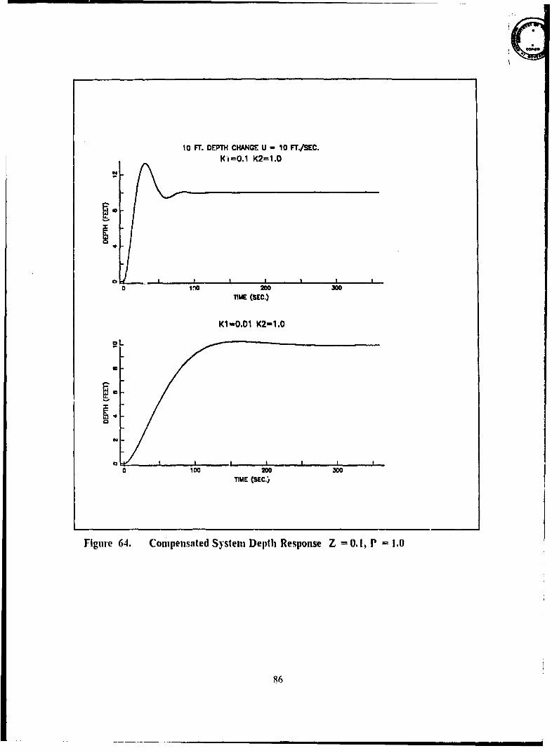
10 FT. DEPTH CHANGE U - 10 Fr./SEC.K'o =0.l K2=1.0

N

0 Io 2WI,'0200 300

IIME (SEC.)

K1-0.01 K2-1.0

e I I I I

0 100 200 300

"MIME (SEC.ý

Figure 64. Compensated System Depth Response Z = 0.1, P = 1.0

86

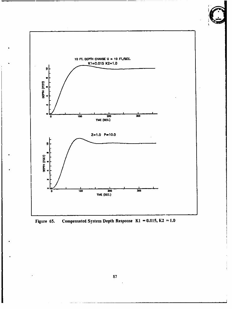
10 FT. DEPTH CHANGE U - 10 FT./SEC.Kt=0.015 K2=1.0

0 1200 300TIME (SEC.)

Z-1.0 P-10.0

BS

a 100 200 300TIME (SEC.)

Figure 65. Compensated System Depth Response KI = 0.015, K2 = 1.0

87

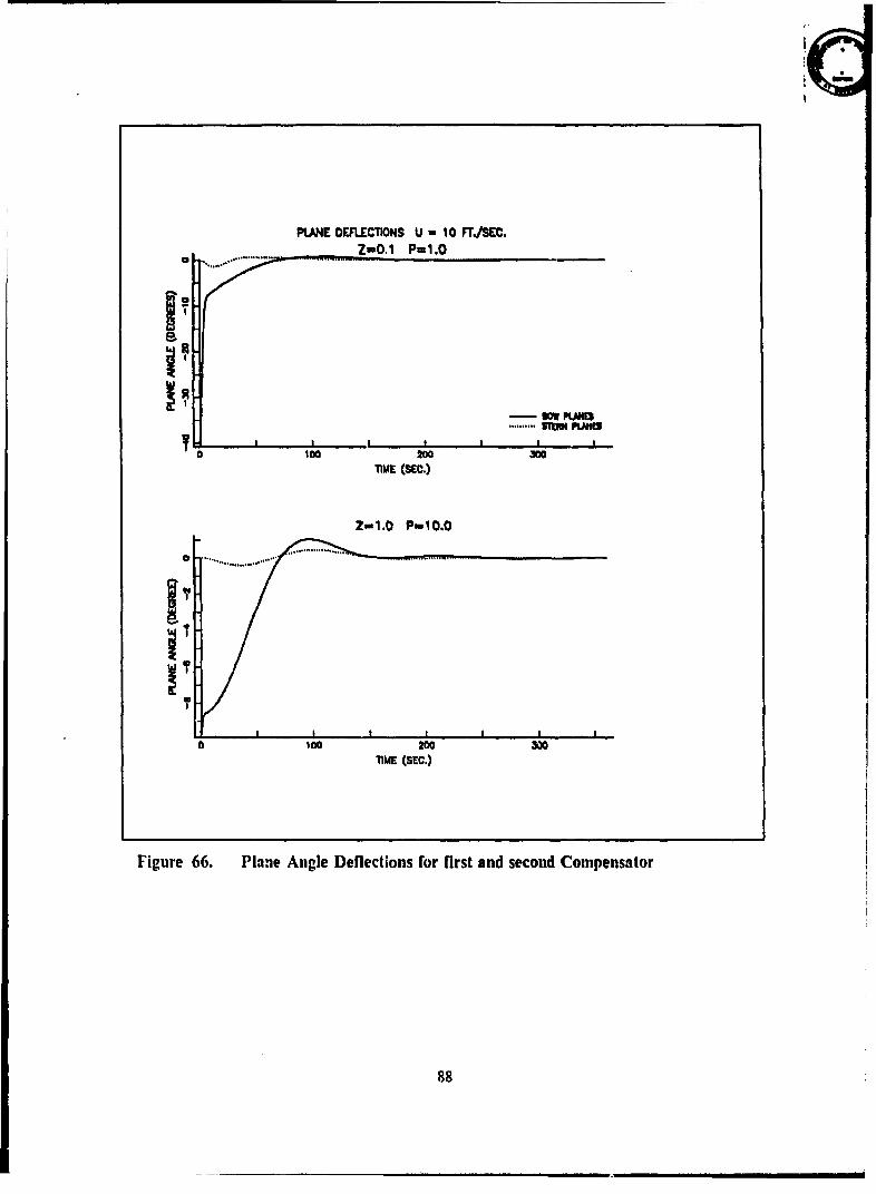
PLANE DEFLECTIONS U ' 10 FT./SEC.Z"0.1 P" 1.0

. .......... . I• RA

100200 300TIME (SEC.)

Z-1.0 P-10.0

? .o. .. ................ .

II I I I , I

010 200 30071ME (SEC.)

Figure 66. Plane Angle Deflections for first and second Compensator

88

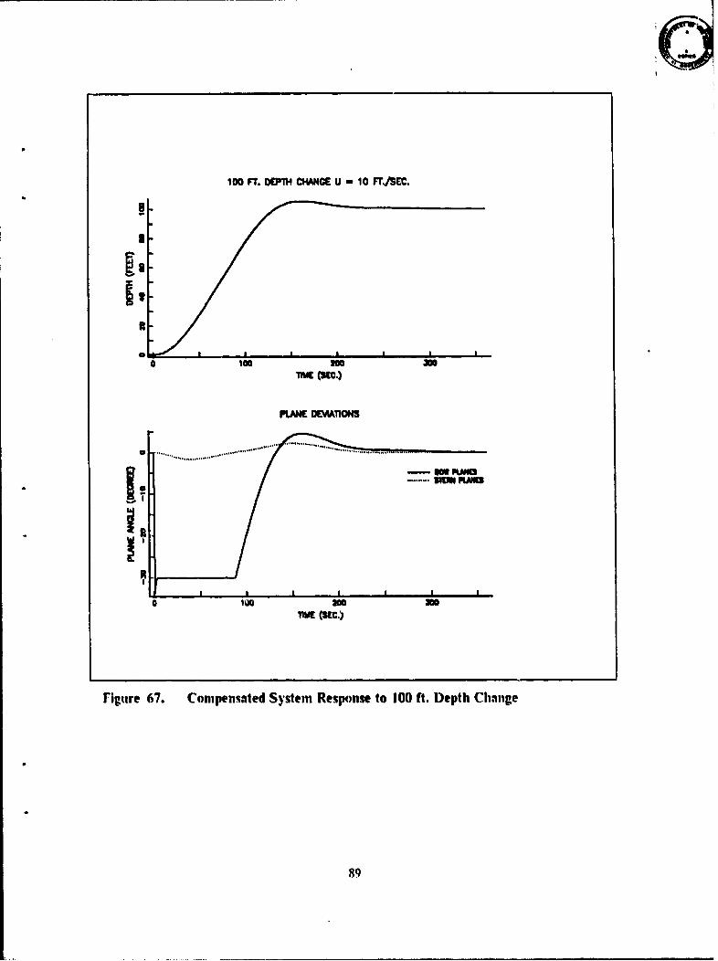
100 F. M0 CHANGE U - 10 Fr'/SEC.

0 oo 300fltU (SEC.)

PLANE DCEdW10NS

o 1o LID1oo 300

TIME (seC.)

riguire 67. Comipensated Systemt Response to 100 ft. Depth Change

89

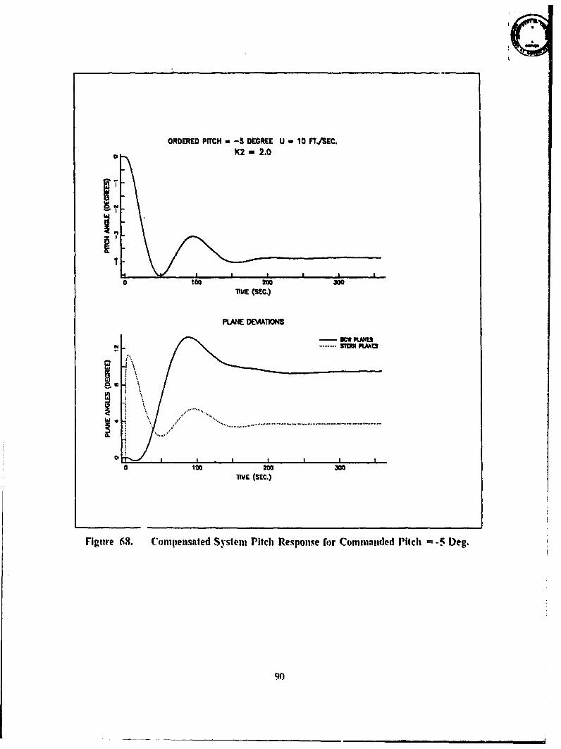
ORDERED PITCH , -5 DECREE U , 10 FT/SEC.K2 -2.0

I'

0 Ica 2w0 300

TIME (SEC.)

PLANE DEMATIONS

I .. .. ...... .......................

a 100 200 300liME (SEC.)

Figure 68. Com!pensated System Pitch Response for Commanded Pitch -5 Deg.

90

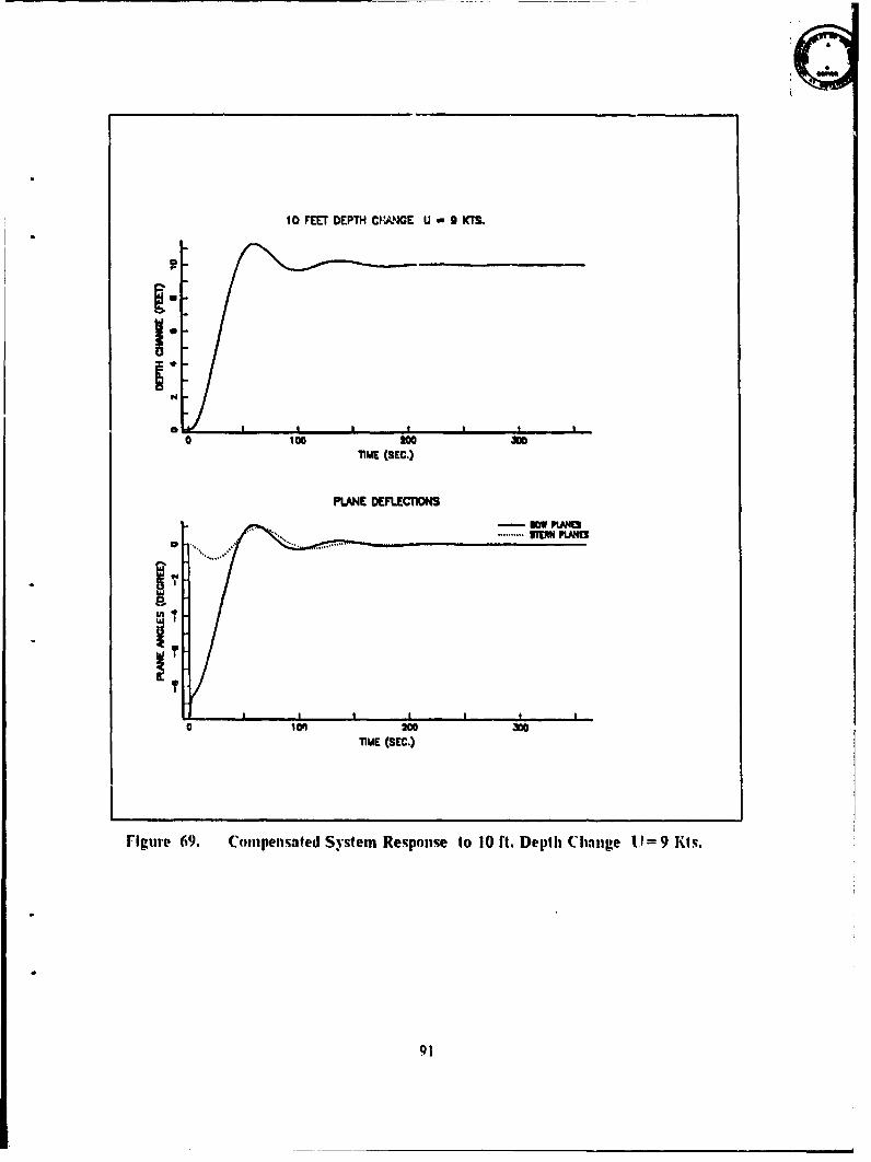
10 FEET DEPTH CMANGE U " B KTM

I- -------

TIME (SEC.)

PLANE DEFLECTIONS

sm pt4

0 Ion 2m000TIME (SEC.)

rigtiie 69. Compensated System Response to 10 ft. Depth Ckuinge 1.1 9 Kts.

91

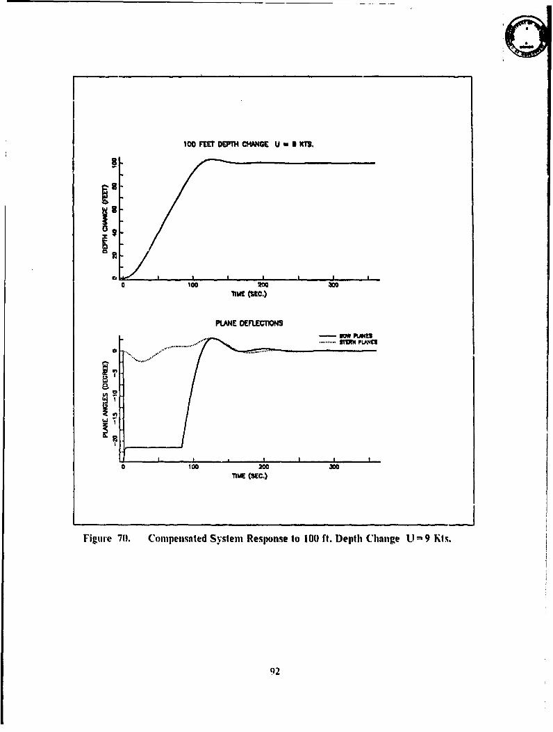
100 FEE1 DEPTH CHANCE U 9 S KXM.

I!ci

0 tO100 300lnME (sEc.)

PLANE DEF'.EClTONS

...

...... .......... ..........

I _ _ _ _ _ _ _ _

01001 2W 3

-nm! (sEc.)

Figure 70. Compensated System Response to 10l) ft. Depth Change LU 9 Kis.

92

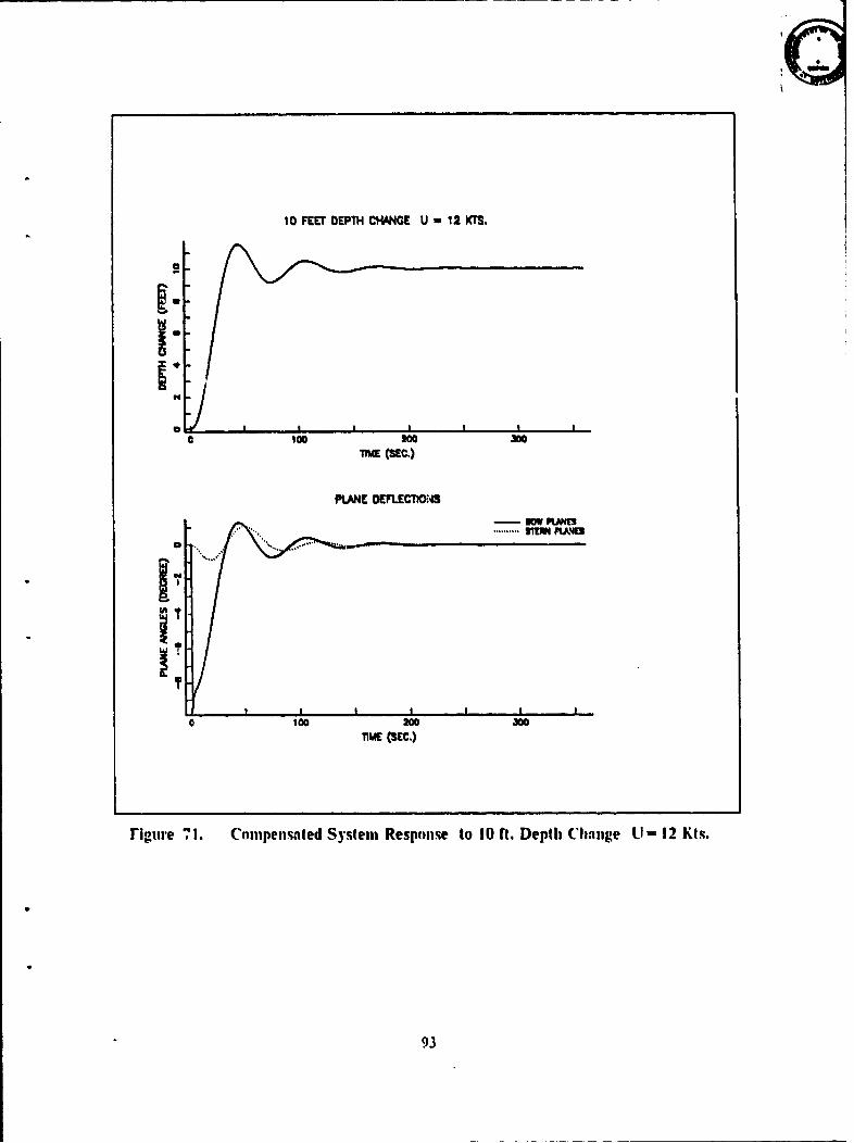
9

10 FEET DEPTH CHANGE U , 12 KTS.

I.wa

0 100 000TIME (SEC.)

PLANE DEFTLECT'ORS- rWl PLANI

T

0 100 Na030TIME (SEC.)

rigu'e 71. Compens•ted System Response to 10 rt. Depth C'hange 1= 12 Kis.

93

100 FEET DEPTH CPANCE U 12 K

o 100 90030

TnME (SC.)

PL.ANE DERECTIKWS

o100 2w 3W

"lME (SEC.)

Figure 72. Compensated System Response to 100 ft. Depth Change U- 12 Kts.

94

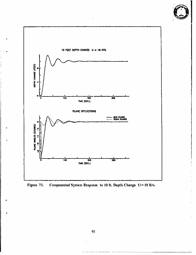
10 FEET DEPTH CHANGE U , 18 KTS.

I-

0 100 200 300TIME (SEC.)

PLANE DEFLECTIONS

I I .. . I I ,

Ic0 200 300TIME (SEC.)

Figure 73. Compensated System Response to 10 ft. Depth Change U= 18 Mts.

95

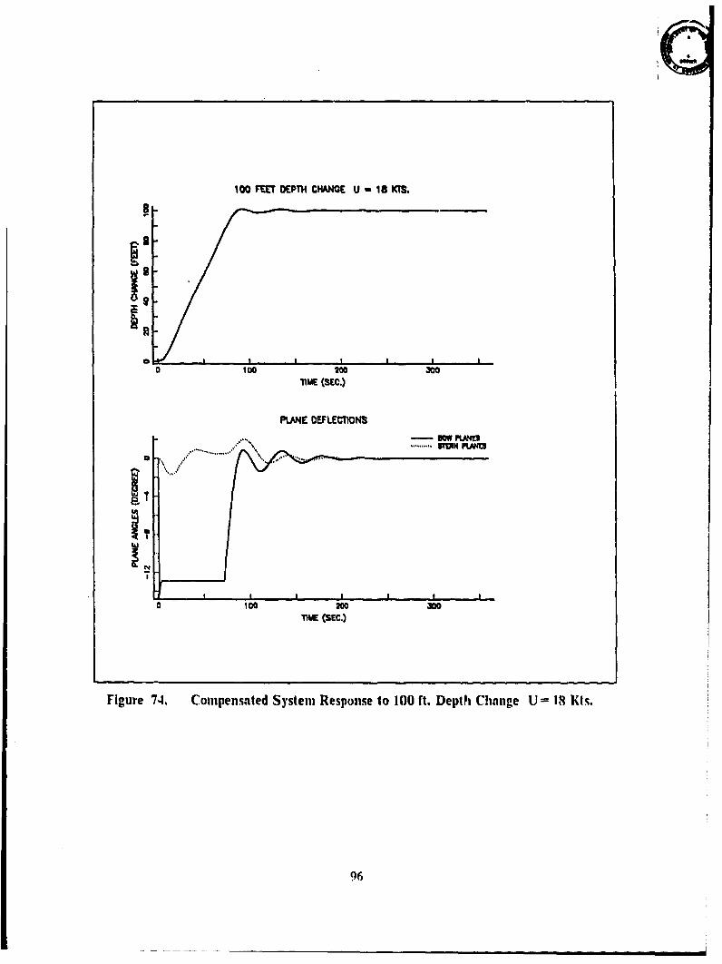
100 FMt DEPTH CHANCE U 1 8B KtS.

0100 200 300"TiME (SEC.)

PLANE DEFLECTIONS

S.,..,,/... ............ WMN• KAM

100 200 300

M1ME (SEC.)

Figure 74. Compensated System Response to 100 ft. Depth Chinge U = 18 Kts.

96

IV. AUTOMATIC STEERING CONTROL

Turning characteristics of a surfaced submarine are very similar to a surfiace ship.

But the situation in the submerged position shows big diflibrenccs. Sail structure can be

considered the main difference and the main source of rolling. But roll control is not

considered in this study since the main purpose was to control depth change which is

caused by the rudder.

In Chapter 2, three equations of motion were linearized and derived for the hori-

zontal plane. Same equations will be used to design a steering control For a submerged

submarine. But the algebraic loop problem has to be solved before using Mason's gain

rule.

Three linear equations for horizontal motion are

= l.89i - 6.3/ - 0.291ur - O.035up; - 2.563xlO-3 uv + 7.568x MO-4 1,Sr (43)

-0.679i - 0.0584" - 8. 179x10- 3up - 9.347x10-3ur -3.942xl- 4 tur

+ 3.942.xlOf510 - 6r - 0.2364) (44)

i= -6.553xl0-3/f + 6.767x10- / - 6.767xl0-3ur -4.51 IxlO-6ol - 4.076xlI0- V4

-1.63 Ix 0l5 u2Sr (.5)

Substituting the highest derivative terms into each equation and after a great deal

of a!gebraic work

' = -0.437ur + 0.027up - 5.06xl4'-4uv + 6.49xlO-4 uSr- 2.399,,h (46)

i, = .021"ll - 9.8x10-3up -3.384x10-'41uv + 1.249x10-su 25r - 0.378,b (47)

= -7.2x1-- ur + 7.Sx1O-Sup -3.888x1O- 5uv - 1.595x10- 5u23r - 4.094x1-1•/3 (48)

A. DESIGN SPECIFICATIONS

In general, the required time to achieve a course change in a ship depends on

1. The forward speed,

2. The diflference between previous and commanded course,

3. Applied rudder angle,

4. Rudder area,

97

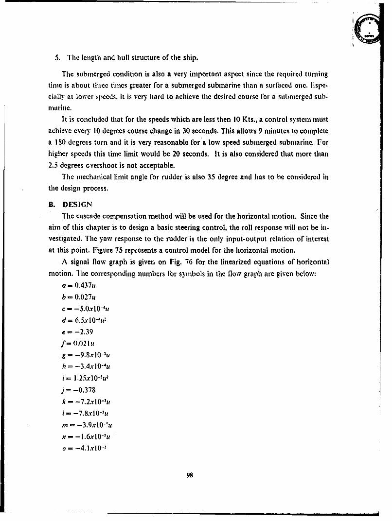
5. The length and hull structure of the ship.

The submerged condition is also a very important aspect since the required turning

timc is about three times greater for a submerged submarine than a surfaced one. Espe-cially at lower speeds, it is very hard to achieve the desired course Flor a submerged sub.

marine.It is concluded that for the speeds which are less then 10 Kts., a control system must

achieve every 10 degrees course change in 30 seconds. This allows 9 minutes to complete

a 180 degrees turn and it is very reasonable for a low speed submerged submarine. For

higher speeds this time limit would be 20 seconds. It is also considered that more than

2.5 degrees overshoot is not acceptable.

The mechanical limit angle for rudder is also 35 degree and has to be considered in

the design process.

B. DESIGNThe cascade compensation method will be used for the horizontal motion. Since the

aim of this chapter is to design a basic steering control, the roll response will not be in-vestigated. The yaw response to the rudder is the only input-output relation of interest

at this point. Figure 75 repfesents a control model for the horizontal motion.

A signal flow graph is giver, on Fig. 76 for the linearized equations of horizontal

motion. The corresponding numbers for symbols in the flow graph are given below:

a = 0.437u

b = 0.027u

c.= -5.0x I 0-4u

d = 6.5x10-4u2

e = -2.39

f= 0.02 11u

g = -9.8x10- 3uh = -3.4x10- 4u

i= 1.25xlO-Iu2

j = -0.378

k - -7.2xlO- 3ui - -7.8xlO-:u

in = -3.9xl0-i:

n = -l1.6xl-u

o= -4.1xlO- 3

98

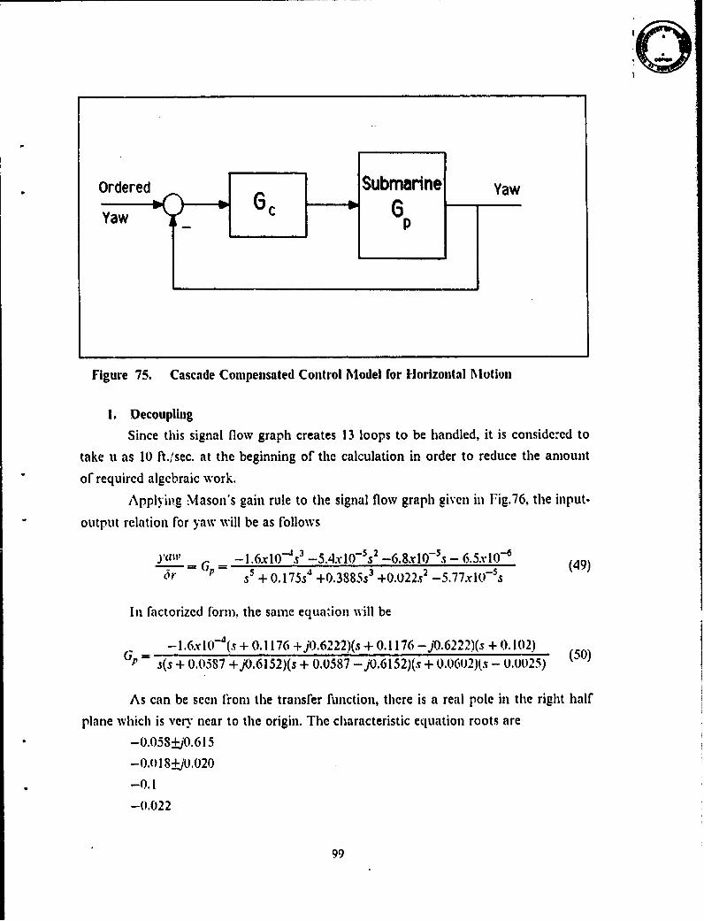
0

Ordered Submarine YawYaw C G P

Figure 75. Cascade Compensated Control Model for Horizontal Motion

1. Decoupling

Since this signal flow graph creates 13 loops to be handled, it is considered to

take u as 10 ft./sec. at the beginning of the calculation in order to reduce the amount

of required algebraic work.

Applying Mason's gain rule to the signal flow graph given in Fig.76, tile input-

output relation for yaw will be as follows

y = -_ 1.6x(.V'10-.S'_5.xl0-s 2 -6.8xl0(-s - 6.5xlO(4

6 r = s5 + 0.175s4 +0.3885s3 +0.022.s2 -5.77x.o- 5s

In factorized form, the same equation will be

-l.6xi0)-(s + 0.1176 +j0.6222)(s + 0.1176 -jO.6222)(s + 0. 102)GP - s(s + 0.0587 +j0.6152)(s + 0.0587 -jO.6152)(s + 0.0602)(s - 0.0025) (50)

As can be seen from the transfer function, there is a real pole in the right half

plane which is very near to the origin. The characteristic equation roots are

-0.05S+j0.6 15

-0.0 1 8_,0.020

-0.1

-(0.022

99

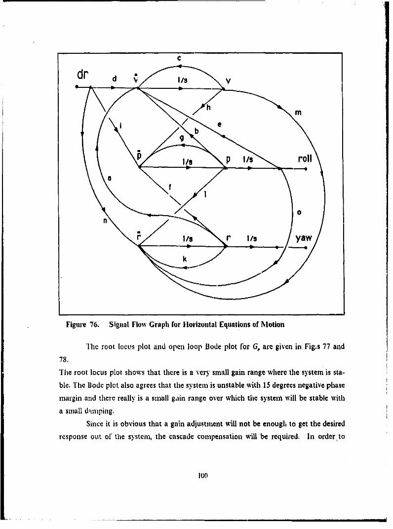
C

dr" 1d , v

b

P p /S roll

I/ . .. _ /yaw

Figure 76. Signal Flow Graph for Horizontal Equations of Motion

The root locus plot and open loop Bode plot for G, are given in Fig.s 77 and

78.

The root locus plot shows that there is a very sm-all gain range where the system is sta-

ble. The Bode plot also agrees that the system is unstable with 15 degrees negative phase

margin and there really is a small gain range over which the system will be stable with

a small damuping.

Since it is obvious that a gain adjustment will not be enougl to get the desired

response out of the system, the cascade compensation will be required. In order to

100

YAW/RUDDERNO COMPENSFTOR

c-

1 * 0 1 ,,..•(I - - j-'-w r-•w

U

, 'OF

* I - - - - - -6S

a

U,,-0•-0.I -O -S 0I -0.0 -OO' -O.S -O.,L ,10OO

REAL AXI S-

Figure 77. Root Locus Plot for --.

1r0

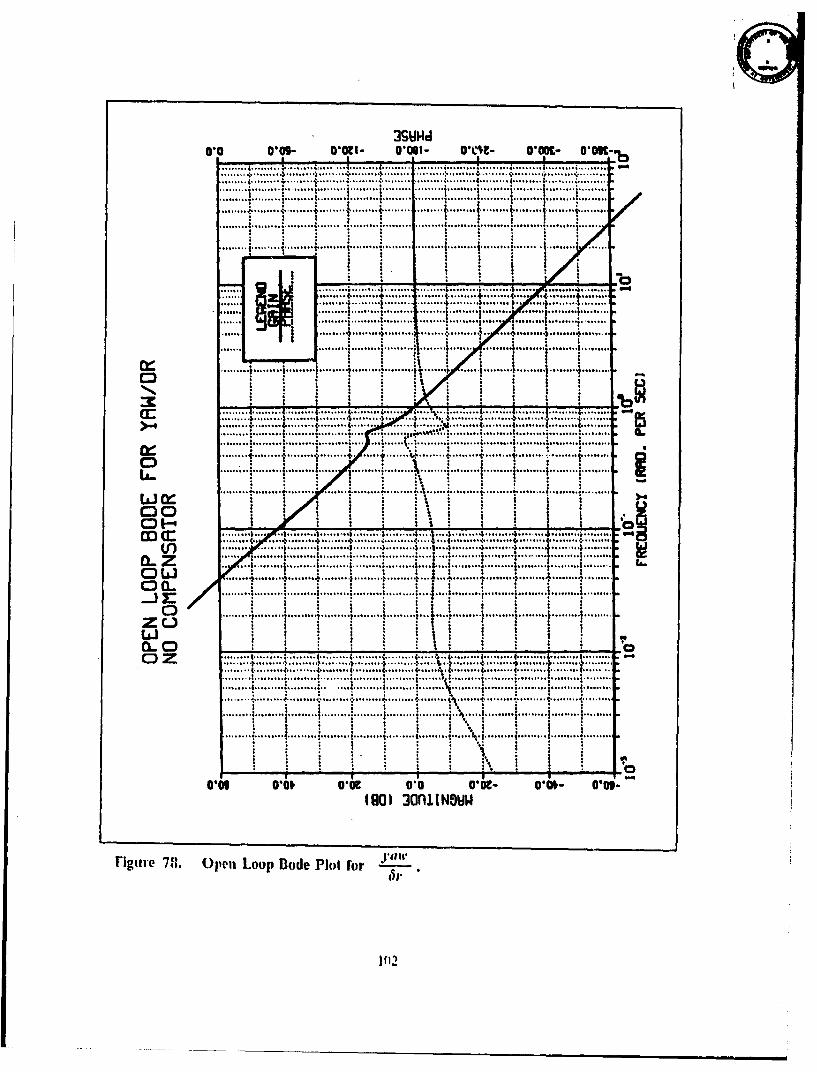
3SY14d

0"0 0009- rOlc1- O010t- 0001- 0'O 0OKI-.4 .............. ........... ................... ,.......... ......... .

,, *. ,'" • , ", "* " ......... . ; . . .......... .:...... ... ! '...... ....... * .. , ......... .,l....,.,. ......... , ......... .. ........ . *......... ........ •.......... ..... . .. |........ I ........ . . . .. .,......... I ......... . ........................ ............. I...............I. ........ ......... .........

... .......

............ .... ........ ........ ........ ......... .................. ........S......... $.......... ......... •........ ......... . ....... I ........ !......... ......... 1......... 4......... •........ .

S..... .Z.... .. : ...... .. ........ ....... ,.*'........... , ......... I., ... ,, ,-, ,* *,,.*... ... . , .. .... . . .. 4.. ... ........... ......... ......... ......

.... ,T ; I . ......... .. . . ......... .. .. .. .... ... .. .. . ....... .. . ........ ; . ,. .... i..... ....... .. ......... . ..........

• .,,, I•I • ~r .. •,,.4 .. .... , ....... ....... - ......... I. .. ... I, •,.•e...... . ........ ..........- * , ..............

S...... - .. ....... . ........ ....... .......... ..... . . . ... ..... ÷ ..... .S............... : ........ i ..... ,.... ...... • ...... ......... ......... i ............ .......... ............... ..."• i ! ! i i isa~i i

CC. ......... ... .;. . . ..... .... . ..... . . ......

S ........S..... i......i......"......... .... t '....... :, " " . ......... i......... i ........ . ..... ..!......... C ......=.. ....i......... ......... "T -'". . - ......... ;......... •.......... " ...... *. ......... ..........c........ ...... . ........ ........ ......... ........ I ......... ........ .

S.................. ............. ...... ......... .

.. . ...... ...... ....... ..... ........ .. . ...... . ......... .

111"I~~~~~~ (I .... '• .... i.. ..•,, ..".......... I,,.. ,..... .; .i..... ....... .. ........M T ..... , , .* .*•. ....... • ........ ... , ,. ...... . *.:.****......... *. ........ .. , .*.

. ..................... , ........ .... *.....a _ z ......... ......... ...... ,....:......... ......... ....... ...... ......... ......... .0 ....... .... .. ..... ......... 4...•,. ........ . ...... .....$ ......... :.........

. . . , • • . I000..... ......... i ......... ......... ......... ......... . '-÷.."......... i ........ ......... ......... !....

' ,, I....... . . . . . . .. . ..

..................... ......... .. ..................

. 4 . . . . ... .............................. ......... ........ . ......... ......... .. ........ .........S.... . I. ... . . ......... :.......... " ......... ......... ........$ ......... % ......... :.........1. .......... ................... ......... . .......... ..... .... ......... .. . ....... .. . ...... .I ......... i ........ .......... I ......... .... .

... ........... ..... ,. ........." 2! ! S ".I :I............. '.............. .

0"09 0"0 0"0C 0.0 0".6- 0"4- 0.09-(01 30nIINSUW

Y7,,,.Figure 78;. Openi Loop Bode Pint for ,---

l f 2

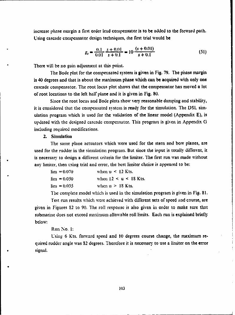
increase phase margin a first order lead compensator is to be added to the forward path.

Using cascade compensator design techniques, the first trial would be

0.1 s+0.0I _ 0 (s+0.0 1) (51)g"0.01 s+O.I 10- .

There will be no gain adjusment at this point.

The Bode plot for the compensated system is given in Fig. 79. The phase margin

is 40 degrees and that is about the maximum phase which can be acquired with only one

cascade compensator. The root locus plot shows that the compensator has moved a lot

of root locations to the left half plane and it is given in Fig. 80.

Since the root locus and Bode plots show very reasonable damping and stability,

it is considered that the compensated system is ready for the simulation. The DSL sim-

ulation program which is used for the validation of the linear model (Appendix E), is

updated with the designed cascade compcnsator. This program is given in Appendix G

including required modifications.

2. Simulation

The same plane actuators which were used for the stern and bow planes, are

used for the rudder in the simulation program. But since the input is totally different, it

is necessary to design a dilflcrcnt criteria lor the limiter. The first run was made without

any limiter, then using trial and error, the best limiter choice is appeared to be:

lim = 0.070 when u < 12 Kts.

lirn =0.050 when 12 < u < 18 Kts.

lia = 0.035 when u > 18 Kts.

The complete model which is used in the simulation program is given in Fig. 81.

Test run results which were achieved with different sets of speed and course, are

given in Figures 82 to 90. Tlhe roll response is also given hi order to make sure that

submarine does not exceed maximum allowable roll linmits. Each run is explained briefly

below:

Run No. i:

Using 6 Kts. forward speed and 10 degrees course change, the maximum re-

quired rudder angle was 82 degrees. Therelore it is necessary to use a limiter on the error

signal.

103

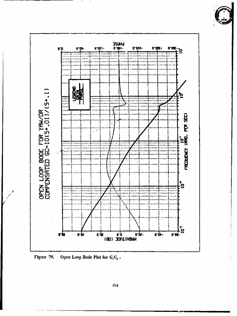
0.0 0102- *O1t- O109t- WOWO 0100c- 00l~...................__ ___ ___ __ 1 ............ ........ 1 i - . .a

p .........

................. ......

.. . . ... . .. ............. .... .% ... .. ........

* 1..... ............ ................ ..

L nI .. . ..1 .... . . . . ..... .. 1.. . .

1 . ... ........ ....... ....

.................... ....

O J .. ..... ..... .....

.4 .4..........

4f.............. ......... . . .

*L )1 - i ........ .... .... . . ........ ..... ... ...

a ......... .

D...... ..4............ ............. ~.. .. ......

Li .1........ . 4. .....

0 - ..... ..... ....

....... 7 7 ..... 1.4.

0-O6 Olat 00 0*G- 010)- 01M-(9013 OfIINSUU

rigure 79. Open't Loop Bode Plot for G,(;,

104

m9in.

uma�mCOMPENSATED YAW/DRGC-5�O.O1/S�O. 1

'.5- a -- - - - - -S

- - *� La...

* - ( --

US S

- a aU

SS

S

UU)

US

.1 - - -- ---* (3- aS

S

UUS - - - a - a

* - - -

* a

a* -

- a

-oaa.o.an otis -otis -o.iw -o.o7s -o. -0.m 0.000 @.mREAL AXIS

Figure 80. Root Locus Plot ror 6. G,.

I �J5

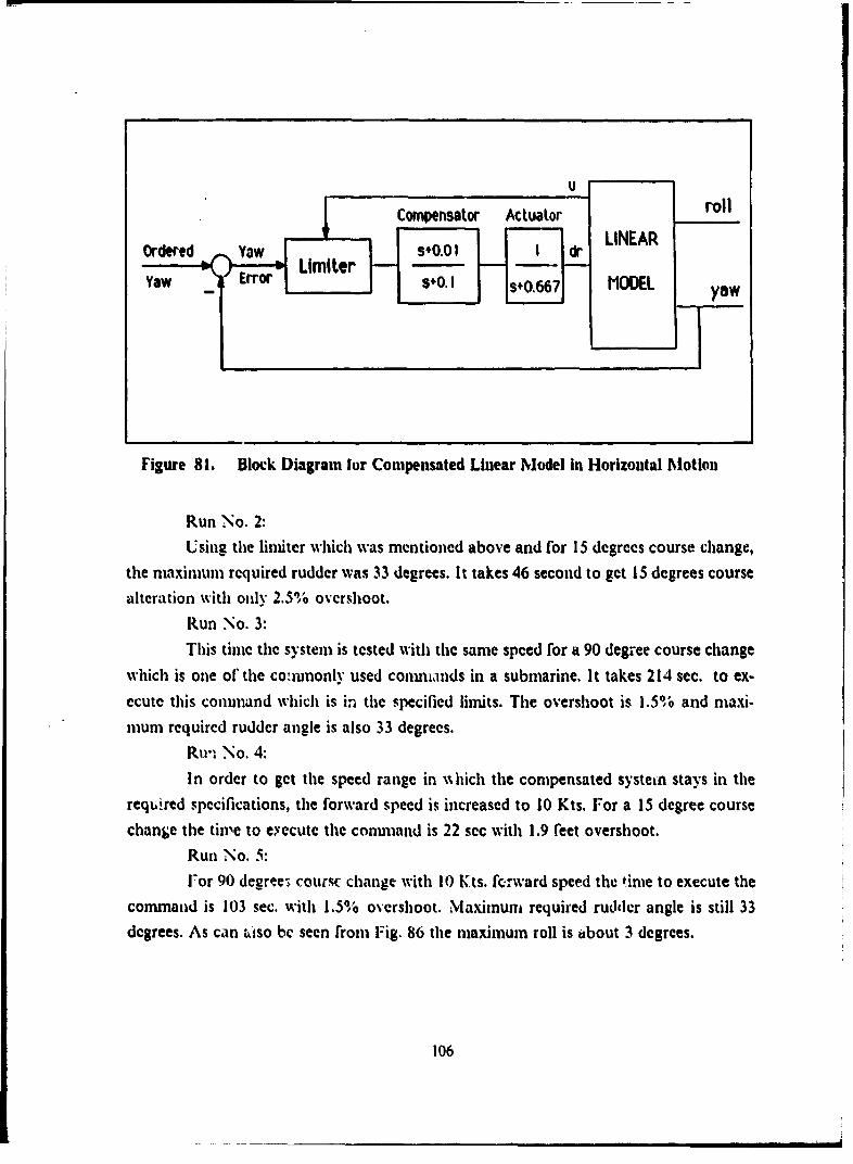
U

SComnpensator Actuator rollOree Ya S+.0 1 .I. INAor~ eo ) errrw Lim iter ' -;

Yaw Erro S+.o. s#0.667 MODEL w

Figure 81. Block Diagram [or Compensated Linear Model in Horizontal Motion

Run No. 2:Using the limiter which was mentioned above and for 15 degrees course change,

the maximum required rudder was 33 degrees. It takes 46 second to get 15 degrees coursealteration with only 2.5% overshoot.

Run No. 3:This time the system is tested with the same speed for a 90 degree course change

which is one ol'the co:3nonly used continands in a submarine. It takes 214 sec. to ex-ecute this conimand which is in the specified limits. The overshoot is 1.5% and maxi-mum required rudder angle is also 33 degrees.

Ru'n No. 4:In order to get the speed range in ahich the compensated system stays in the

requiired specifications, the forward speed is increased to 10 Kts. For a 15 degree coursechange the time to e.ecute the command is 22 sec with 1.9 feet overshoot.

Run No. 5:For 90 degree7 coursc change with 10 Kts. f.rward speed the time to execute the

command is 103 sec. with 1.5% overshoot. Maximum required rudder angle is still 33degrees. As can tiso be seen rrom Fig. 86 the maximum roll is about 3 degrees.

106

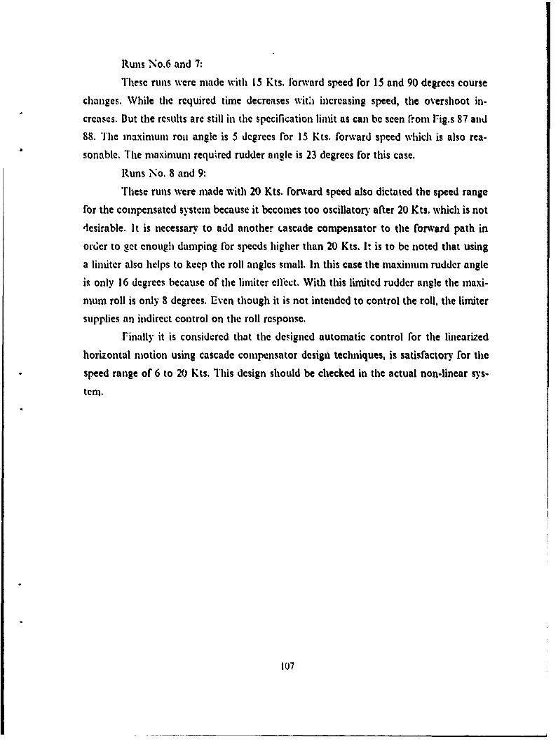
Runs No.6 and 7:

These runs were made with 15 Kts. forward speed for 15 and 90 degrees course

changes. While the required time decreases with increasing speed, the overshoot in-

creases. But the results are still in the specification limit as can be seen from Fig.s 87 and

88. The maximum ron angle is 5 degrees for 15 Kts. forward speed which is also rea-

sonable. The maximum required rudder angle is 23 degrees fbr this case.

Runs No. 8 and 9:

These runs were made with 20 Kts. forward speed also dictated the speed range

for the compensated system because it becomes too oscillatory after 20 Kts. which is notdlesirable, It is necessary to add another Lascade compensator to the rbrward path in

order to get enough damping for speeds higher than 20 Kts. It is to be noted that using

a limiter also helps to keep the roll angles small. In this case the maximum rudder angle

is only 16 degrees because of the limiter ellect. With this limited rudder angle the maxi-

mum roll is only 8 degrees. Even though it is not intended to control the roll, the limiter

supplies an indirect control on the roll response.

Finally it is considered that the designed automatic control for the linearized

horizontal motion using cascade compensator design techniques, is satisfactory for the

speed range of 6 to 20 Kts. This design should be checked in the actual non-linear sys-

tem.

107

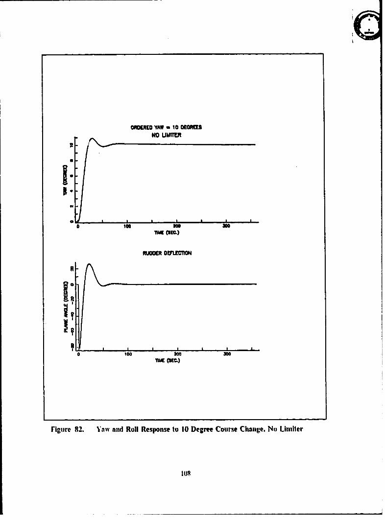
OROMREO YAW W 10DEORS

NO UMITER

30

RUOOW CFI.ECllO

I.i

o Ia 2w 30

TIM (SEC.)

Figure 832. Ya•w and Roll Response to 10 Degree Course Chang~e. INo) Unifer

I;)

ORDERED YAW 1S DEREES - U m KYS

Y AW

o ... "i ........ ........ ............... .•" . .... ............. ............... l,0 104 IN0 300

7mE (SEC.)

RUDOER OEFLECTION

0 100 200"71ME (SEC.)

Figure 83. Y'aw and Roll Response to 15 Degree Course Change. Wilh Limiter

1U9

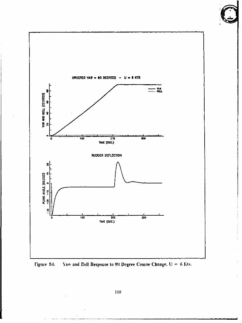
ORDERED YAW-go DECREES - U - KS

= ....... .. .. ...*.......". ....& ...... ~.................. 4...........

0 IDon 210 3O

TIME (SEC.)

RUDDER DEFLECTION

3 0

0 100 200TIME (SEC.)

rigure 8|4. Yi'i and [oll Response to 90 Degree Course Clihige. U(. 6 EI..

ll0

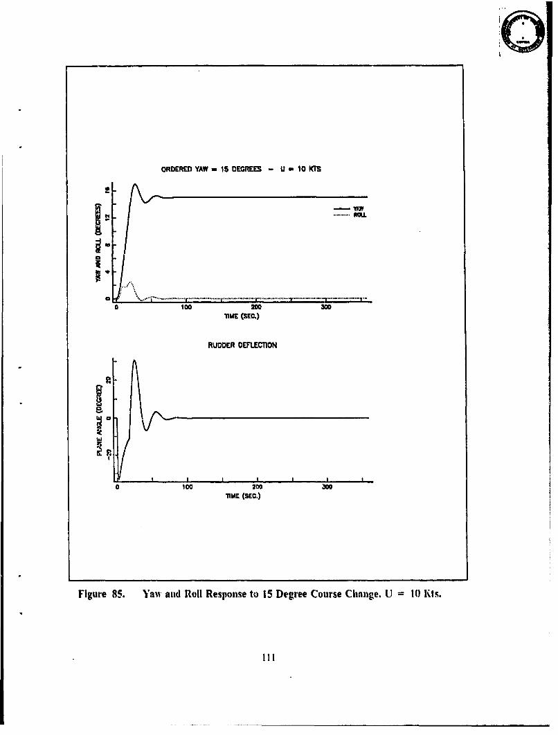
ORDERED YAW w 15 DEGREES - U W 10 KTS

.. . .. .............. .. ............. ........... . . . ..... -... .........

100 200 300M1ME (SEC.)

RUDDER DEFLECTION

0 100 200 300TIME (SEC.)

Figure 85. Yam- and Roll Response to 15 Degree Course Chnnge. U = Mo) Ks.

II

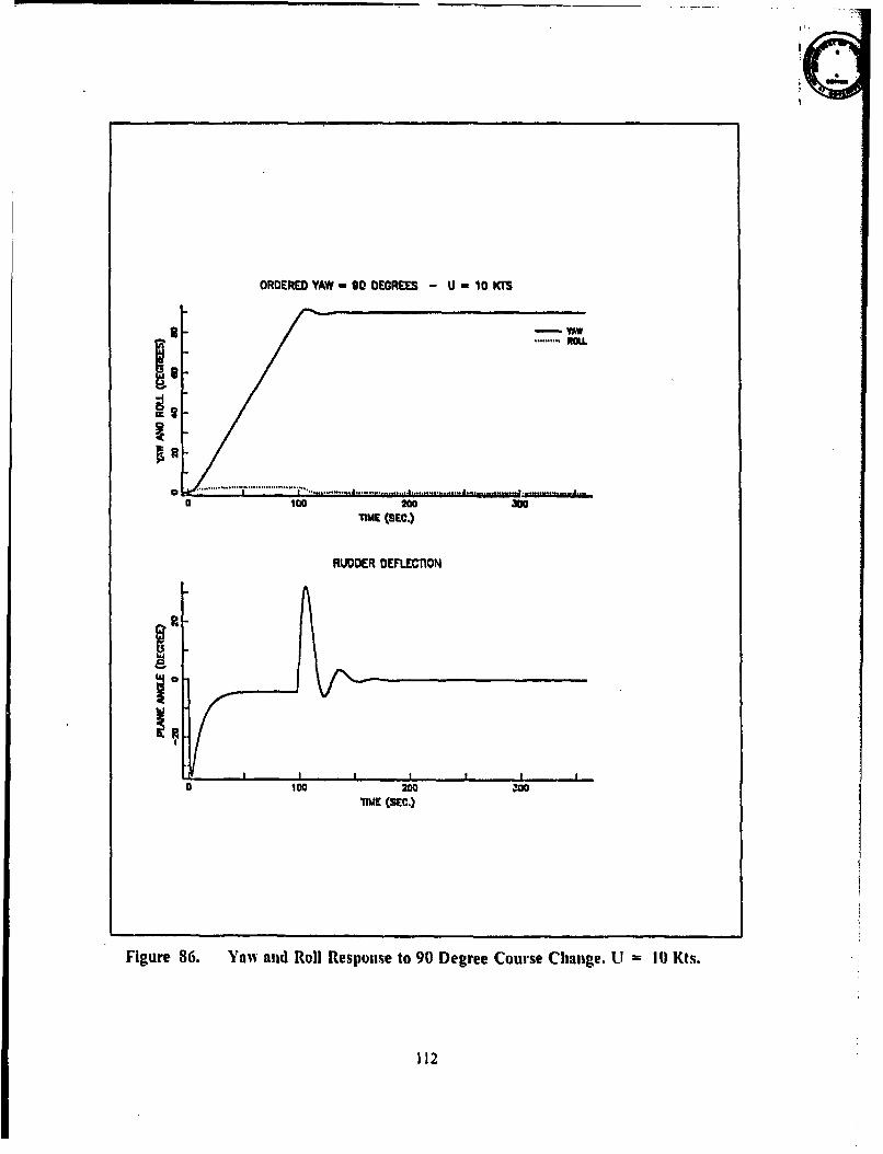
4

ORDERED YAW O0 DEGREES - U 10 KS

3

0 100 2w 300TIME (SEC.)

RUDDER DEFLECTON

NO10 200 300-nME (SEC.)

Figure 86. Yaw and Roll Response to 90 Degree Course Change. U I0 Kts.

112

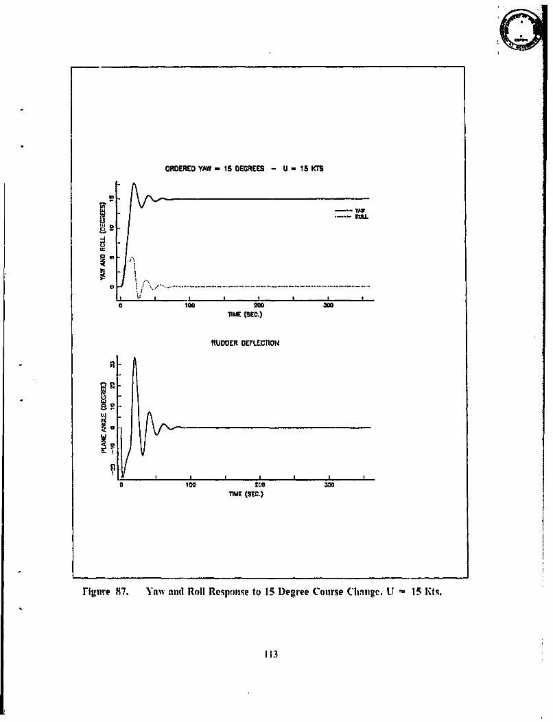
ORDERED YAW , 15 DEGREES - U - 15 KTS

Is

o ... .............................. .................................. ..... ...................... ................. ...... ....... ....... ....

100 200 30OTIME (SEC.)

RUDDER DEFLECTION

C3 .

0 100 200 30TIME (SEC.)

Figure 87. Ymnw and Roll Response to 15 Degree Course C.hnge. U - 15 Ki.s.

113

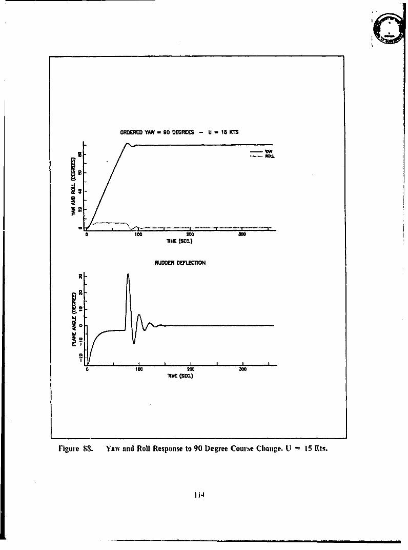
ORDERED YAW - 00 DEGREES - U m 15 KTS

S...... ..... ...... .. ..... * .........-.. ..

a 100 20o 3oW

TIME (SEC.)

RUDDER DEFLECTION

'a'

S100 200 300limE (sEc.)

Figure 88. Yaw and Roll Response to 90 Degree Course Change. U = 15 I(ts.

114

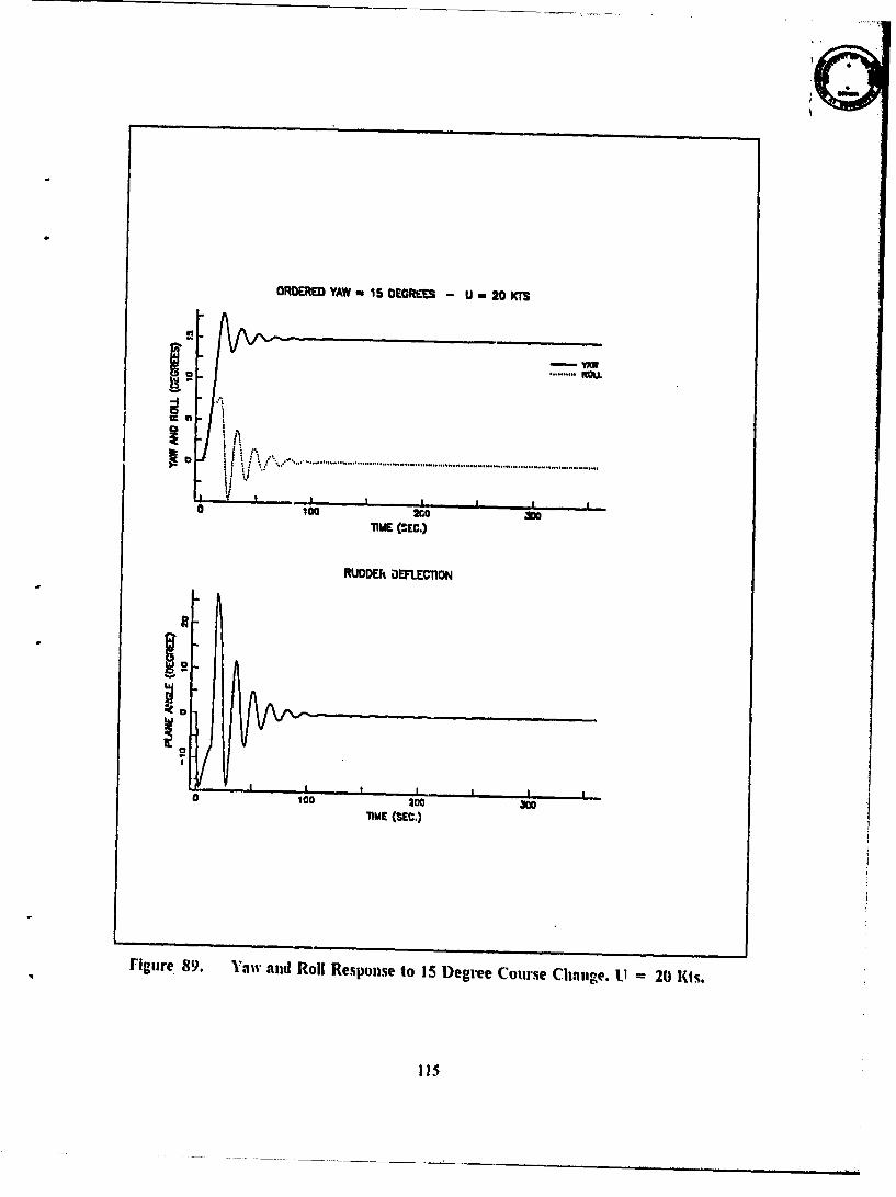
ORDERED YAW - 15 DEGREES - U - 20 KTS

... . ............. .......................

•lhE (SEC.)

RUDDER DEFLECTION

0 100 200 300WiE (SEC.)

rigure 89. I'm" and Roll Response to 15 Degree Course Ch.uige. 11 20 I(ts.

115

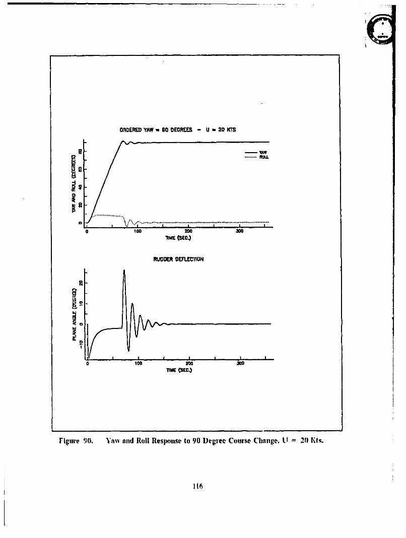
ORDERED YAW 2 00 DEGREES - U , 20 KTS

. /':,.. ..... ..... .... .......... .. . . ................................

0100 no0 3w0

71ME (SEC.)

RUDDER DEFLECION

Ica0 2w0 300limE (SEC.)

Figure 90. Yaw and Roll Response to 90 Degree Course Cl.hange. U 21 0Is.

116

V. VALIDATION OF THE COMPENSATED NON-LINEAR MODEL

Tlhc main purpose or this study was to show that it is possible to design acompensator bascd on the linearized version of a non-linear model and then to com-pensate the actual non-linear model with this designed compensator. In the previouschapters the required compensators were designed for the linear models on vertical andhorizontal motions. These compensators had to be checked with the actual non-linearmodel to see that the system will really work with them.

The complete DSL simulation program for the non-linear model was alheady writtenand used by Rer. 3 and Ref. 5. It is also used for this study to compare linearized modelswith the non-linear model. In order to check the validity of automatic control systems,the DSL simulation program is to be modilied including the compensator and limiteralgorithms in it. The modified version of the DSL program ror the compensated non-linear model is given in Appendix 1.

A. SIMULATIONFor the test runs to check the designed compensators, the same limiter values are

used. Since the actual and commanded velocities ( U and UC ) are two dillercnt pa-rameters and U is always somewhat less then UC, it is concluded to take actual speedU as the paramctcr ror the limiters. This will give more accurate plane dellections de.

pending on actual Forward speed.The ,i on-lincar simulation program was run at 6, 10, 12, 15 and 20 Kts. For various

depth. pitch and yaw commands. A diving submarine can give hundreds of maneuvervariations in three dimensional motions. Since it is not possible to include all n" them:only the most common conunands and the commands which were used in Chapter 2.3and 4 -ire included For comparison purposes.

The trim values for the ordered speed arc carefully calculated ICom Rer. 5 and im-plemented in the non-linear model.

Test run results which were achieved for different sets of specds and commands aregiven in Figures 91 to 106. Each run is explained briefly below:

Runs No. 1-4:Tihe simulation program was run for 10 and 100 ft. depth changes at 6 Kts. com-

mnanded forward speed. As can be seen from Fig. 91 thle non-linear model completes a10 ft. depth change 10 sec. after the linear model does. It completes a 11m) It. depth

117

change 210 see. alfer tile linear model and overshoots ror both case are onl the spcilica-

tion limits. There is also a I ft. steady state error for both cases.

At the same speed the simulation program was run for I5 and 91) degree course

changes. As can be seen from Fig. 92 the non-linear model takes about fIM) seconds to

achieve a 15 degree course change with no overshoot and a slight undcrshoot. Also the

required time to make a 90 degree course change is more than 360 seconds lor the non-

linear model. These two case are also non-acceptable.

The main reason for this failure is the decreasing forward speed due to the planedellections. The forward speed, depending on the amount of the rudder deflection, ac-

tually drops up to 4 Kts. while achieving a course change maneuver. The same thing also

happens for a depth change maneuver due to the szern and bow planes. The

compensators were designed for actual 6 Kts. and higher speeds and they do not meet

the specifications for less than 6 Kts. forward speed.

Under these circumstances no more investigations were made at 6 Kts. At this point

it is concluded to operate at 10 Kts.

Runs No. 5-8:As can be seen in Fig. 93 the non-linear model completes a 10 Il. depth change in

42 seconds with I ft. overshoot at 10 Kts. It completes a 100 11. depth change in 106seconds with 3.5'!% overshoot. These numbers satisfied the required specilications and

,' :v are nearly the same as 'or the linear model with a little time lag.

As can be seen in Fig. 94 the non-linear model makes a 15 degree course change in25 seconds with 0.8 degree overshoot which is less than the linear case. For a 91) degree

course change the time is 205 seconds with no overshoot. Again due to the rudder drag

force. the time to reach the commanded course is much larger but more realistic than the

linear •, e. Since the constant speed assumption which is used for the linear model is

no longer valid for large perturbations, this is really expected. On the other hand thed,-, -:d cascade compensators can still control the actual non-linear system elliectively

eilu and in l 'ct. with less overshoot which is very important from the point of' this

stud'

Runs No. 9-i2:

In o, er to have an idea about speed deviation due to the plane dellections, four

runs were perl'ormed for 10 and I(M) feet depth change and 15 and 90) degree course

change ,L 1. Kts. As can be seen in Fig. 95 there is an appreciable dillUrence betweenthe drag forces created by rudder and bowistern planes. This is expected since the rudder

has a lot more surihee than the other planes. For a 15 degree course change the forward

118

speed drops abruptly to 9.3 Kts. and goes back to it's original value in a relatively smalltime. [or a 90 degree course change. the forward speed drops up to 9 Kts. and sta's al.most constant for about 150 seconds which is the greatest cause lor the slower courrc

change rate.

Runs No. 13 and 14:Since the linear model assumes no cross-coupling between vertical and horizontal

motion, these runs are performed only for the non-linear model. Cross-coupling ellectson depth and pitch angle are shown in Fig. 96 at 10 Kts. for 15 and 90 degree coursechange commands. For both commands, the submarine stays in the 5 fkct depth and 2

degrees pitch error limitations.

Run No. 15:

One of' the most difficult maneuver for a submarine is to change depth whileachieving a course conunand. Results of such a maneuver are given on Fig. 97 and Fig.

98. A simulation run For simultaneous 91) degree course and I(H) Il. depth chanige corn-mands. shows that the time to reach 90 degree course change is about 40 seconds longerthan the usual condition but it does not allect the depth change. Because or the rudderel1ect only a small depth error appears until the submarine settles on the desired course.

As can be seen in Fig. 98 the non-linear submarine's roll and pitch responses arcsomewhat non-regular but still in reasonable limits for this case. The forward speed de-

viation due to the plane drag forces is also given in Fig. 98. Speed drops up to 8.3 Kts.and this givcs an explanation for lower course change rate.

As a result For this run, even though the designed control systems interact, they canwork well simultancously.

Runs No, 16 and 17:

In order to be able to compare fixed rudder effects on depth and pitch angle. twosimulations were pcrformcd for 15 degree aad 35 degree fixed rudder commands in thesame fashion as in Chapter 4 at 12 Kts. For 15 degree rudder the pitch and depth errorsstay in specified limits but For 35 degree rudder these errors are not allowable. Simulation

results Ior this case are given in Fig. 99.Runs No. 18 and 19:Figure It•W gives the simulation results for a 15 and a 90 degree course change at 15

Kts. for both linear and the non-linear models. The yaw response For 15 degree coursechange is almost the same as the response for 10 Kts. with a little more overshoot andoscillation. On the other hand the non-linear model shows a better response with less

overshoot for both cases.

119

Runs No. 20 and 21:Figure 101 gives the simulation results for a 10 and a 100 feet depth change at 15

Kts. Surprisingly there is almost no difference between linear and non-linear model forthe 10 I~et depth change. But for the 100 1I. depth change the non-linear model has a

faster response than the linear model. This is unusual and created by differcnt lihiterbehaviors on bow planes at this specific forward speed.

Runs No. 22 and 23:In a real submarine a depth change conunand usually comes with a pitch command

in order to reduce the time to get the desired depth. Figure 102 gives the results of sucha command for 100 feet depth change with 5 degree down pitch angle at 6 and 15 Kts.

For both cases the submarine reaches the desired depth 35 seconds bcfore the case forwhich no pitch comnmand is given. But as a trade-off the overshoots are over 10%. Alsothe pitch command has to be reduced to zero before the desired depth is reached in orderto avoid too much overshoot and a steady state error on depth. This is done 10 Neetbefore the desired depth is reached. for 6 Kts and 50 feet before for 15 Kts.

Runs No. 24 and 25:Finally the compensated non-linear system was checked at 20 Kts. For a 15 and a

90 degree course change, the yaw responses of the compensated submarine are given inFig. 103. Once again the non-linear model gives a better but slower response then tlelinear model. For the 15 degree course change the yaw responses of both models becometoo oscillatory due to the high speed. But the compensator still works well enough tocontrol the submarine.

Runs No. 26 and 27:Figure 104 gives the compensated submarine depth responses for a I0 and a 100 lIect

depth change at 20 Kts. There is a 0.8 feet steady state error for both cases which iscreated by the system dynamics due to the high speed. The control system design isbased on 10 ft.,'scc. ( 6 Kts.) forward speed. At 20 Kts. the transfer functions whichdescribes the submarine dynamics might have very different characteristics. Conse-quently it is concluded that the upper speed limit for this design is 20 Kts. In fact, thecontrol system works up to 25 Kts. without exceeding design specification limits.

The compensated submarine pitch responses for the same runs are given in Fig. 105.The linear and non-linear models show very similar pitch behavior and pitch angles donot exceed the given 2 degree limit even for this high speed.

As a result o1" this chapter it has been shown that the designcd automatic controlsystem for the linearized model can also work effectively on the actual non-linear model.

120

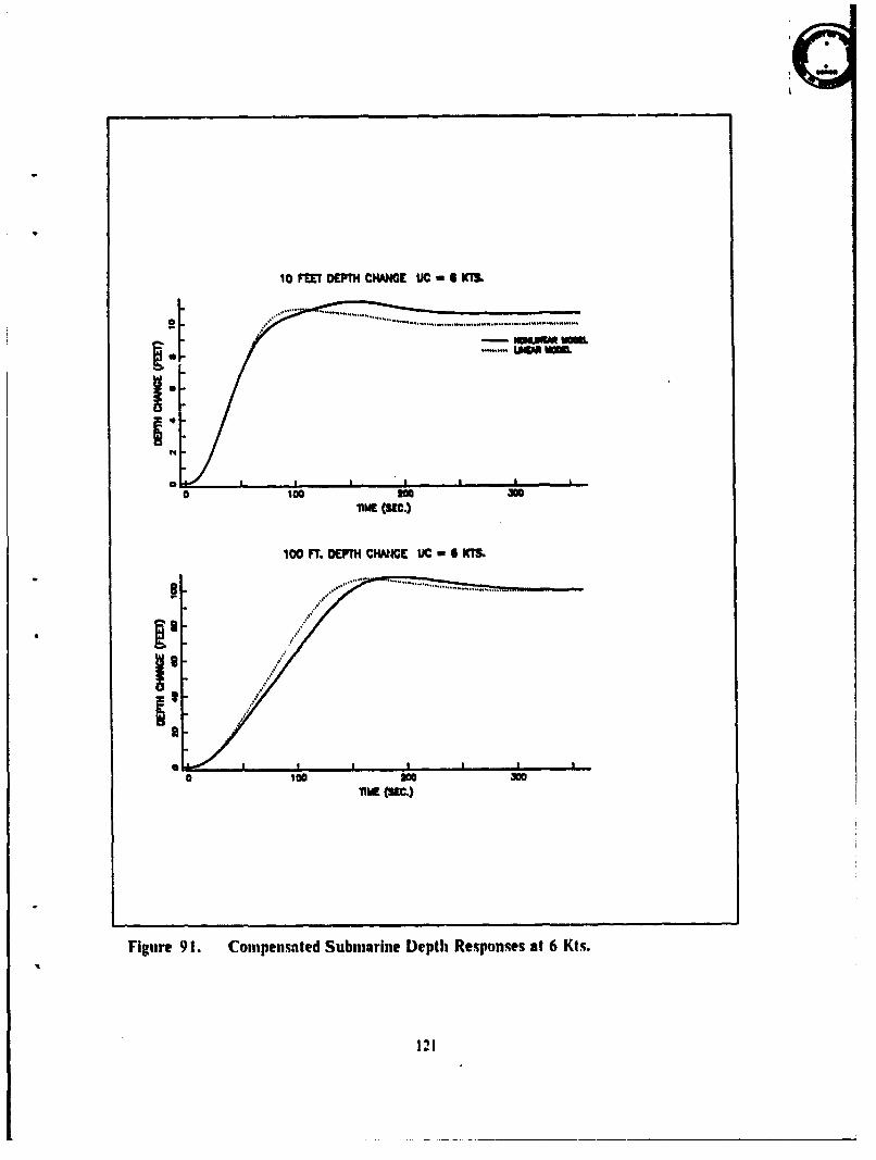
10 F'MT DEPTh CHANGE UC - I KTS.

.. .. .... ... ..... .. .... .. .....,

100 3m •"nIM (SEC.)

100 Fr. DEFTH CHANGE tIC I KIM

a !c o

a 100 2o0 300liME (Nc.)

Figure 901. Compensated SubCmrne Depth Responses at 6 Kts.

14

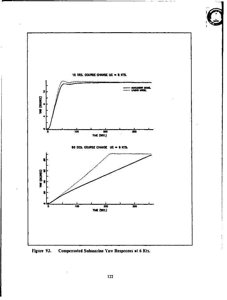
1S OEM. COURSE CHANGE IC- KTM.

- ~umpo LV

0 100 200 300

90 OW. COURSE CHANCE UC =I SKTS.

Figure 92. Compensated Submarine Vaw Responses at 6 Kts.

122

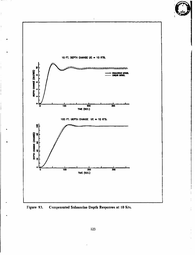
10 FT. DEPTH CHANGE UC - 10 K'M

I.,0 100 10 300

-MIE (SKC.)

100 FT. UEPTH CHANGE UC - 10 KTS.

0 100 200 300TIME (SEC.)

Figure 93. Conmpensated Submarine Depth Responses at 10 Kts.

123

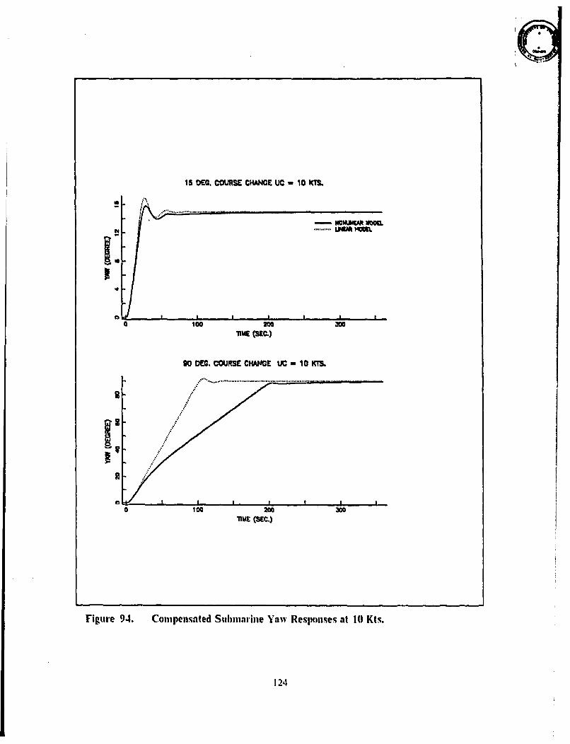
15 DEC. COURSE CH"E UC 1 ¶0 KIM

,'4

.......... tJNr MO M

n100 20 300

TIME (SEC.)

90 DEO, COURSE CHACE UC - 10 KTS.

. . ........................ ...... ....

0 100 200 300

Figure 94. Compensated Submarine Yaw Responses at I0 Kts.

124

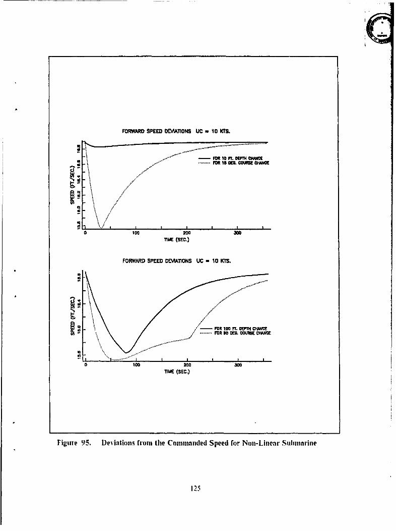
FORWARD SPEED DEVIATIONS UC - 10 KTS.

............. - -....... ..o . ...

, ......... •........... .........

Ica0 200 300

TIME (SEC.)

FORWARD SPEED DEVIATIONS UC -10 KrS.

-! MRI 100 FT. 7fl CIWJ0

6 .. ..... ..

-q MFR 30 0(0. COMJE CH1AN0

..............

\ /

0 100 200 300

TIME (SEC.)

Figurie 9-5. Deviations from the Commanded Speed for Non-Lineir Submarine

125

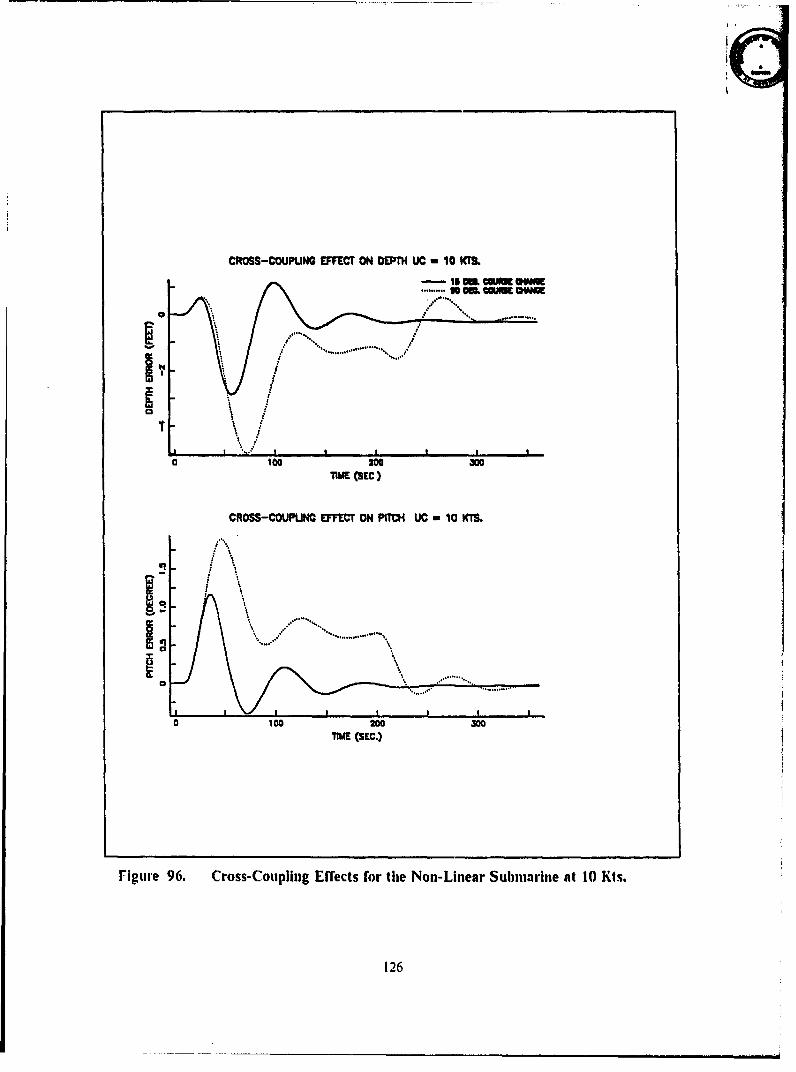
CROSS-COUPUNG EFFECT ON DEPTH UC - 10 KM9

S.......... i l tCH N

0A 100 30030TIME (SEC.)

CROSS-COUPUNQ EFFECT ON PITCH UC 1 0 Kil.

.%

oloo 200 300TIME (SEC.)

Figure 96. Cross- Coupling Effects for the Non-Linear Submarine at 10 Kts.

126

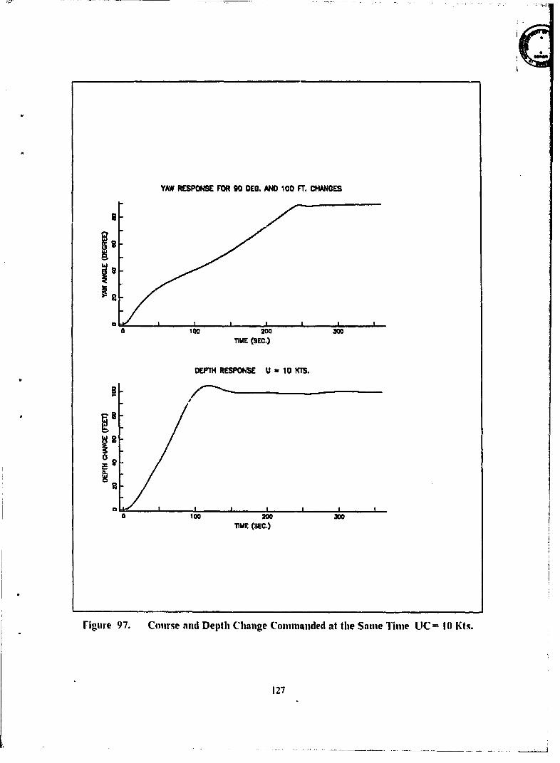
YAW RESPONSE FOR 90 DEC. AND 100 FT. CHANCES

0 100 200 300TIME (SEC.)

DEPTH RESPONSE U " 10 KTS.

I

100 200 300TIME (3EC.)

rigure 97. Course and Depth Change Commanded at the Same Time LIC= 10 Kts.

127

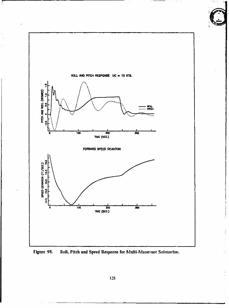
ROLL AND PITCH RESPONSE UC - 10 KTS.

° i ,," ...............

...... ... H

o 100 200 300

iMME (SEC.)

FORWARD SPEED DEVIATION

0 100 200 300

MlE (SEC.)

Figure 98. Roll, Pitch and Speed Response for Multi-Manevuer Submarine.

128

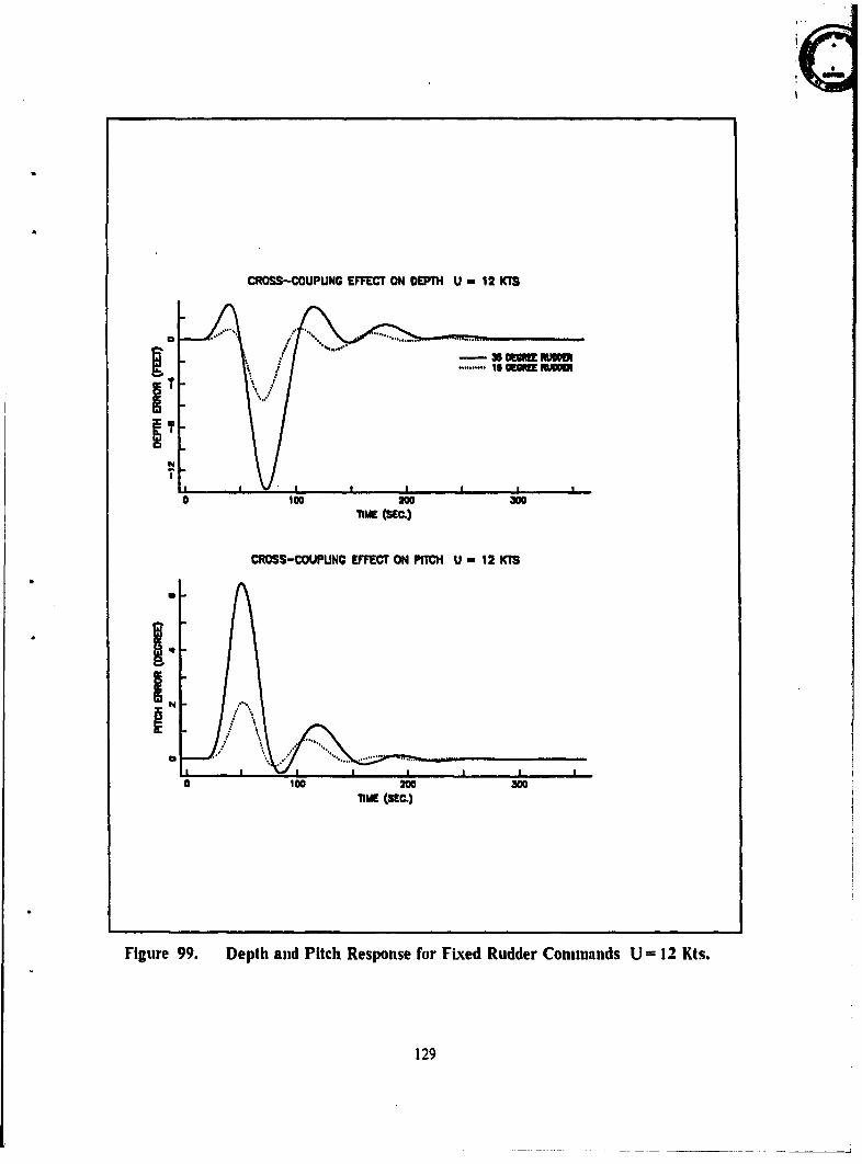
CROSS-COUPUNG EFFECT ON DEPTH U - 12 KTS!... ... .......

0 100 030TIME (SEC.)

CROSS-COUPUNG EFFECT ON PITCH U U 12 KMS

71ME (SEC.)

Figure 99. Depth and Pitch Response for Fixed Rudder Commands U = 12 Kts.

129

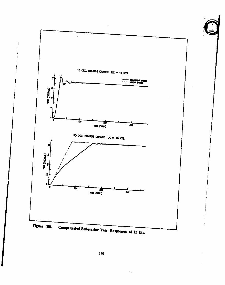
15 DEC' COUSEa CHANCE IC 13 isMu

90 OEQ. MJ3LRS CHANGE UC 13 Cr&~

Figure I oo. Contpensatei Submarine Yllw Responses at 15 Kts.

130

0

10 Ft. DEPH CHiNCE U 1" KTSm .......... UlMM LMML

Tim (Me.)

100 FT. DEPTH CHANCE U - 15 K1

Tom (MC.)

Figure 101. Compensated Submarine Depth Responses at 15 Kts.

131

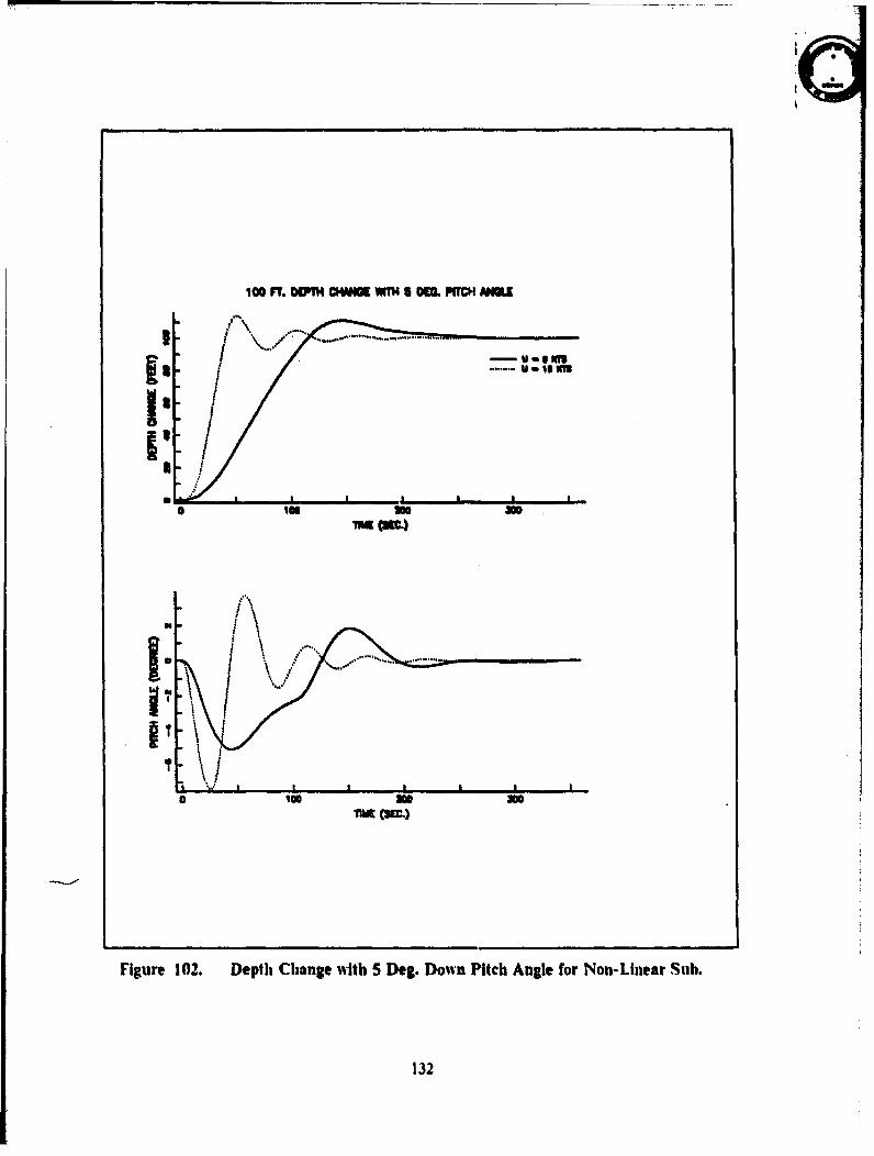
S

100 FM. 90e1WM.CE C IN' WM 5 M. PITC11 AD.K

I 1 . ....... .

a'

'r /

no 300

Figure 102. Depth Change with 5 Deg. Down Pitch Angle for Non-Linear Sub.

132

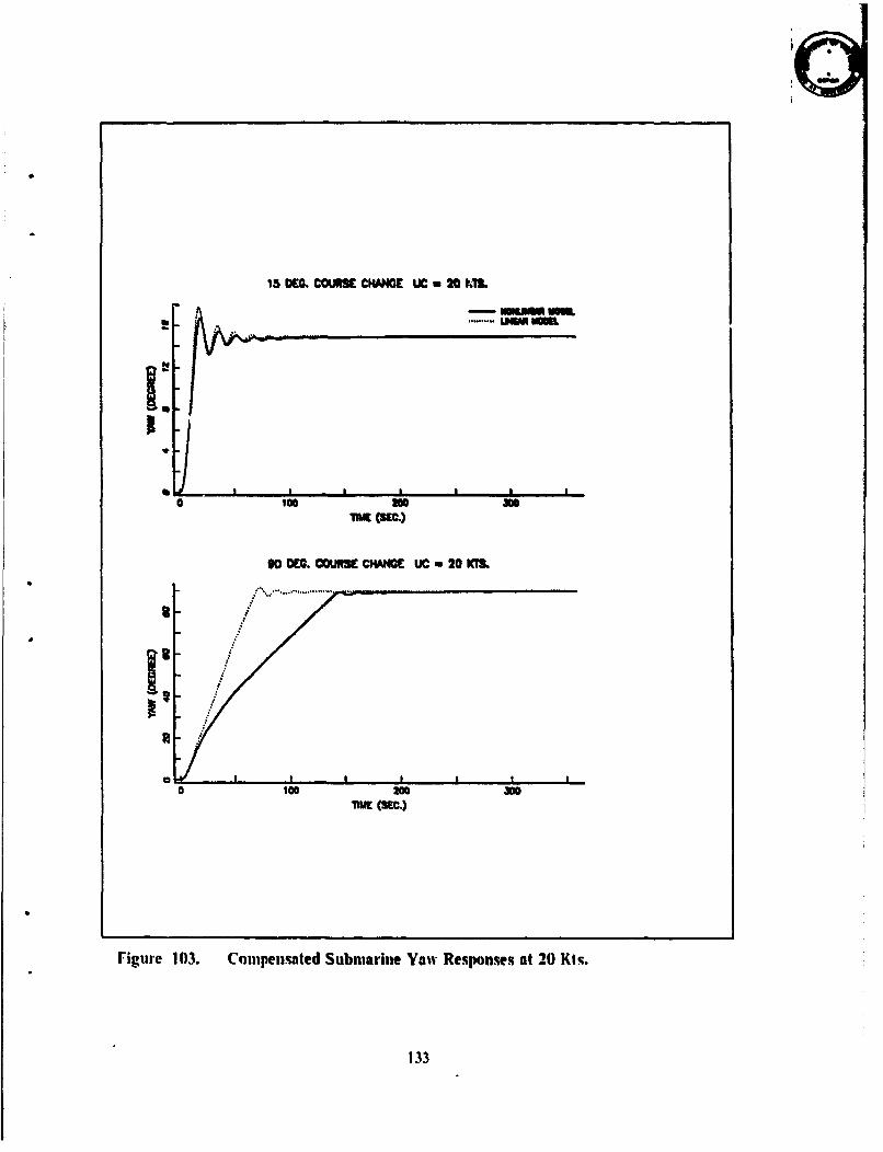
15 DEC, COU. CHANCE UC -,20 K1 .

in

11w (3C0.)

9O DEC. COURS CHAN4CE UC 2 20 KTS.

a taoma0100 2wO 300

1MME (SEC.)

Figure 103. Compensated Submarine Yaw Responses at 20 Kts.

133

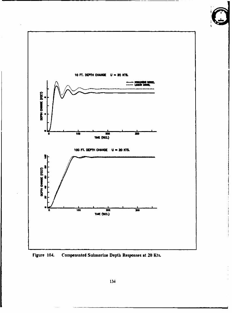
t0 FT. 0BH CHANCE U -20 KMW:WI

101) M UPI CHANCE U-20 KM3

a to , I I I100 00 300

MME (Sc.)

Figure 104. Compensated Submarine Depth Responses at 20 Kts.

134

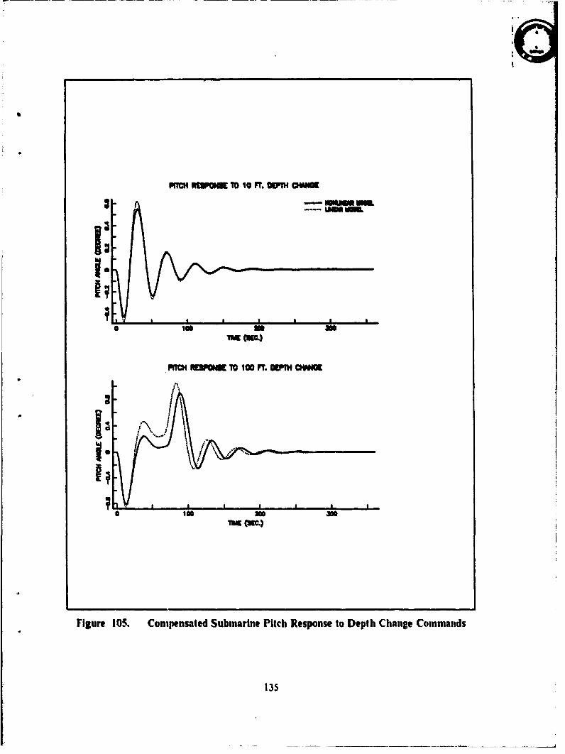
I:IPITCH P 0 1010 FT. OWNTH OWIG

Figure 105. Compensated Submarine Pitch Response to Depth Change Commands

135

VI. CONCLUSIONS AND RECOMMENDATIONS FOR FURTHER

WORK

A. CONCLUSIONSThe linearization o" given non-linear diffeirential equations of motion in six degrees

of freedom, designing two automatic control systems using cascade compensator designtechniques for vertical and horizontal motion of a submarine and finally investigatingcross-coupling effects due to the rudder deflections were the main concerns in this study.

It has been shown that using linearized equations to design an automatic control forthe actual non-linear system is possible for the submarine problem. Also cascade com-pensation, using a single loop technique, which was mainly the Bode plot design in thisstudy, is possible and practical for automatic pitch, depth and yaw control of smallsubmarines.

The designed control systems for both planes satisfied the design specifications fora speed range from 8 to 20 Kts. That means the compensated system is rather insensitiveto speed deviations. Therefore all problems related to gain switching, like cluttering anddiscontinuities in plane angles, are avoided. This is especially important because theforward speed changes significantly during maneuvers.

"The implementation of the designed compensators into hardware has the followingdesirable features:

1. Minimal Instrumentation: Since rate information is not required, no inertial guid-ance system is necessary. Only a regular gyro for course and simple sensors fordepth and pitch angle are needed.

2. Low Cost, Weight and Size: The simplicity of the compensator transfer functionsmakes them easily realizable in physical hardware at low manufacturing cost.Weight and size requirements are very small, another important factor especiallyfor small coastal submarines. A wide speed range is covered by one fixedcompensator and no changes in parameters are necessary.

3. Reliability: The automatic controller can be realized with a set of physical com-ponents with a well known high reliability. High component reliability and a smallnumber of components will generally result in a high system reliability.

B. RECOMMENDATIONS FOR FURTHER WORK1. The designed control system in this study can keep the pitch and depth errors in

reasonable limits for small rudder deflections and course changes. But larger dellectionsstill create an appreciable amount of depth and pitch error at high speeds which is not

136

F6

desirable Ior near surface operations. It might be worthwhile to improve this design toget a sufficient control on cross-coupling effects ror all kinds of heavy maneuvers. This

can be done using dillbrent sets of parameters for the compensators and limiters and.'or

increasing the numbcrs of compensators for the vertical control of the submarine.

2. In some operational conditions it is very important to rmach a desired depth as

soon as possible in a submarine. Therelbre an additional pitch angle command is given

which has an enormous effect on depth change rate. For tile present design it is possible

to give both depth and pitch command at the same time but the watch officer has to

decide where to change the pitch command to zero. Otherwise, depending on the forward

speed and commanded pitch angle, the submarine might not stay on desired depth.

The present design can be modified using a new algorithm which can decide where

and in what fashion to decrease the pitch angle automatically in order to get desired

depth and stay there without any unacceptable overshoot and steady state error.

137

APPENDIX A. DEFINITIONS OF SYMBOLS

SYM IIOL DEFINITION

A dot over any symbol signifies diflerentiation

with respect to time.

B Buoyancy force which is positive upwards.

m Mass of the submarine including thc water in thefree floating spaces.

Overall length of the submarine.

U Linear velocity of" origin of body axes rclativcto an earth-fixed axis system.

u Component of U along the body x-axis.

v Component of U along the body y-axis.

w Component of U along the body z-axis.

ti, Command speed.

x Longitudinal axis of the body fixed coordinateaxis system.

y Transverse axis of the body fixed coordinate

axis system.

z Vertical axis of the body fixed coordinate axis

system.

138

so-

XO Distance along the x axis of an earth-Iixed

axis system.

A Distance along the y axis of an earth-fixcdaxis system.

ZO Distance along the z axis of an earth-fixcd

axis system.

p Component of angular velocity about the body

fixed x-axis.

q Component of angular velocity about the body

fixed y-axis.

r Component of angular velocity about the bodyfixed z-axis.

ZB The z coordinate of the center of buoyance

( CB ) of the submarine.

a Angle of attack.

I? Angle of" drift.

6b Deflection of bow or fairwater planes.

6r Deflection of rudder.

6b Deflection of stern planes.

n The ratio

0 Pitch angle.

139

Yaw angle.

Roll angle.

p Mass density of sea water.

IV, Weight of water blown from a particular

ballast tank identified by the integer assigned

to the index i.

W Angular velocity.

t 'rime.

Location along the body x-axis of the center

of mass of the ilk ballast tank when this tank isfilled with sea water.

(F.), Propulsion force.

I. Moment of inertia of a submarine about the

x-axis.

IY MN!onient of inertia of a submarine about the

y-axis.

Moment of inertia of a submarine about thez-axis.

All K's Non-dimensional constants each of which is assigned

to a particular force term in the equation of motion

about the body x-axis.

All NI's Non-dimensional constants each of which is assigned

to a particular Fbrce term in the equation of m3tion

about the body y-axis.

140

All N's Non-dimensional constants each of which is assignedto a particular force term in the equation o" motionabout the body z-axis.

All X's Non-dimensicnal constants each of which is assignedto a particular force term in the equation of motionalong the body x-axis.

All Y's Non-dimetasional constants each of which is assignedto a particular force term in the equation of motionalong the body y-axis.

All Z's Non-dimensional constants each of which is assignedto a particular force term in the equation or" motionalong the body z-axis.

141

APPENDIX B. HYDRODYNAMIC COEFFICIENTS OF SIMULATION

EQUATIONS

A. AXIAL FORCE

XQQ = -0.000200 XRR = -0.000090 XRP = 0.000250

XUDOT = -0.000150 XVR = 0.011000 XWQ = -0.007500

XUU - 0.0 XVV = 0.006500 XDRDR = -0.002800

XDSDS = -0.002500 XDBDB = -0.002600 XVVN = 0.0XWWN = 0.0 XDR2N = 0.0 XDS2N = 0.0

B. LATERAL FORCE

YP P,'P = 0.0 YPQ = 0.000200 YPDOT = -0.000300YRDOT = 0.000090 YVDOT = -0.011000 YV/R/ = -0.007300YWP = 0.007500 YR = 0.003000 YRDR = 0.0

YIl = -0.000700 YUU = 0.0 YV,'V/ = -0.060000

YV = -0.021000 YDR = 0.006200 YWV = -0.065000

YVS = 0.0 YRN = 0.0 YVN = 0.0

YVAVN = 0.0 YDRN = 0.0

C. NORMAL FORCE

ZRR = -0.001500 ZRP = -0.000900 ZQDOT = -0.000200ZWDOT = -0.007500 ZVR = -0.008000 ZWtiQ/ = -0.006000

ZQ = -0.004500 ZQDS 0.0 ZVP = .0.007000ZUU = -0.000100 ZVV 0.000650 ZVW/'W = -0.030000

ZW = -0.011000 ZDS = -0.005000 ZDB = -0.002500Z,/ = 0.0 ZWW - 0.0 ZVS = 0.4

ZQN = 0.0 ZWN = 0.0 ZWAWN = 0.0

ZDSN - 0.0 Z+VP = 0.0

142

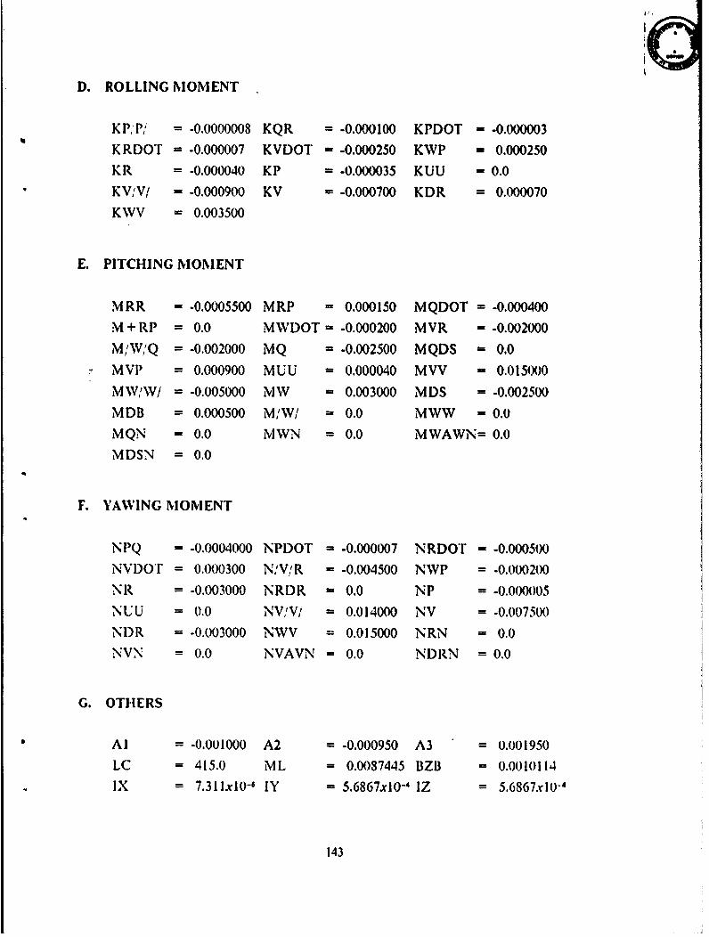
D. ROLLING MOMENT

KP,Pi = -0.0000008 KQR = -0.000100 KPDOT = -0.000003

KRDOT = -0.000007 KVDOT = -0.000250 KWP - 0.000250

KR = -0.000040 KP = -0.000035 KUU = 0.0

KV,,V/ = -0.000900 KV = -0.000700 KDR = 0.000070

KWV = 0.003500

E. PITCHING MOMENT

MRR = -0.0005500 MRP = 0.000150 MQDOT = -0.000400

M + RP = 0.0 MWDOT = -0.000200 MVR = -0.002000

M/,W!Q = -0.002000 MQ = -0.002500 MQDS = 0.0

MVP' = 0.000900 MUU = 0.000040 MVV = 0.015000

MW,'W/ = -0.005000 MW = 0.003000 MDS = -0.002500

MDB = 0.000500 MIW/ = 0.0 MWW = 0.0

MQN = 0.0 MWN = 0.0 MWAWN= 0.0

MDSN = 0.0

F. YAWING NIOMENT

NPQ = -0.0004000 NPDOT = -0.000007 NRDOT = -0.000500

NVDO'r = 0.000300 NV/,RR - -0.004500 NWP = -0.000200

NIR = -0.003000 NRDR - 0.0 NP = -0.000005

NUU = 0.0 NV,'Vi f = 0.014000 NV = -0.007500

NDR = -0.003000 NWV = 0.015000 NRN = 0.0

NVN = 0.0 NVAVN = 0.0 NDRN = 0.0

G. OTHERS

Al = -0.001000 A2 = -0.000950 A3 = 0.001950

LC = 415.0 ML = 0.0087445 BZB = 0.0010114

IX = 7.311x10-1 IY = 5.6867xi0-4 IZ = 5.6867x10-4

143

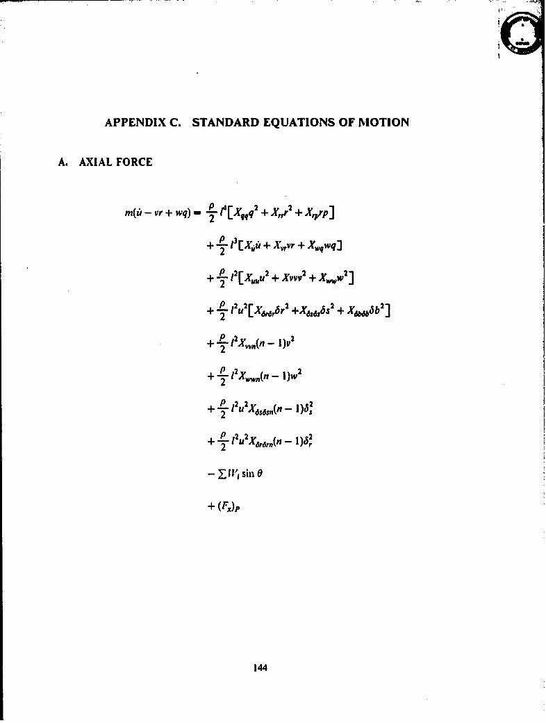
APPENDIX C. STANDARD EQUATIONS OF MOTION

A. AXIAL FORCE

m~ý- vr +wq) - Xq+ Xr 2 + X,,,rp]

+ -~E eXit + Xvrvr +Xwqwqj

+~2Xu~uU2 + XVVV2 + Xw,,2]

+L 11IU2 Xpj~5 2 +X63 ~ s + ~ 2]

+ X,,6 ""3 + u2X6

2 sds,,,n( - I~v

+1!_L 12 2 V (n -I)e52

' 2 £udldr,,,n r

- xfli sin 0

144

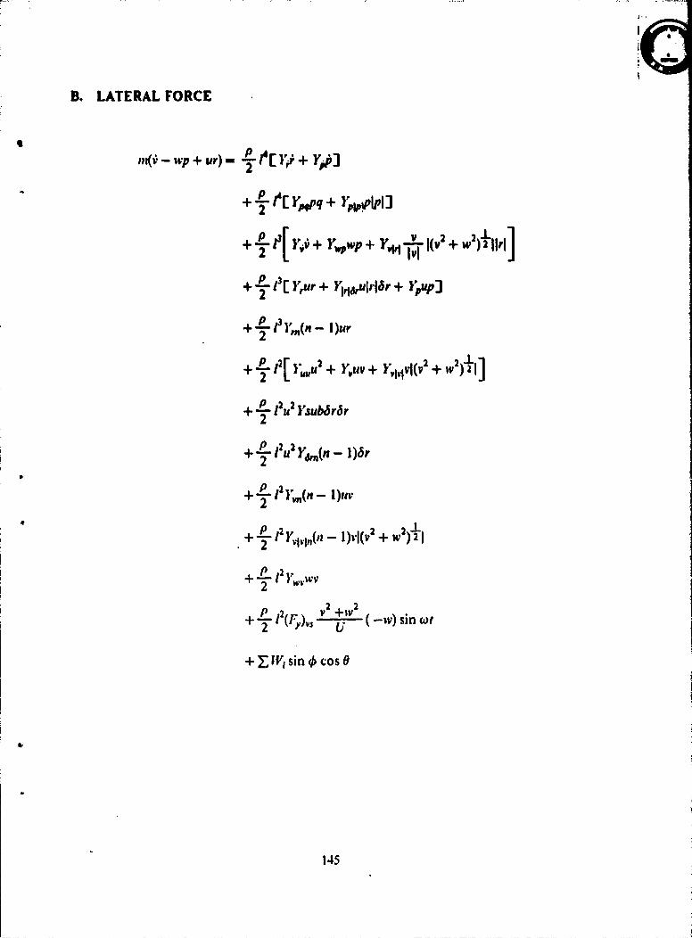
B. LATERAL FORCE

m(- wp + z=r)- L 1r+ Yop]

+ E Yppq + Y ,kplI

2 I3YO1+ Ywpwp + YVrI(Y2wI ArI+ -L 13[ Yur + Y4rgulri6r + Y;up]

2

2 Y 1 r(n - I)ur

+ L 12 1' u + Y•uv + ;,,jvI(v 2 w)2±]

+ _ 12u 2 Ysub6r6r2

+ _L 12U2 y&.(n _ 1)6r

+ _L 12}1, (n -- I)uv

12, w2) 1

+ + w

2

+ T `" (-w) sin wt

+ FWY sin rcos 0

145

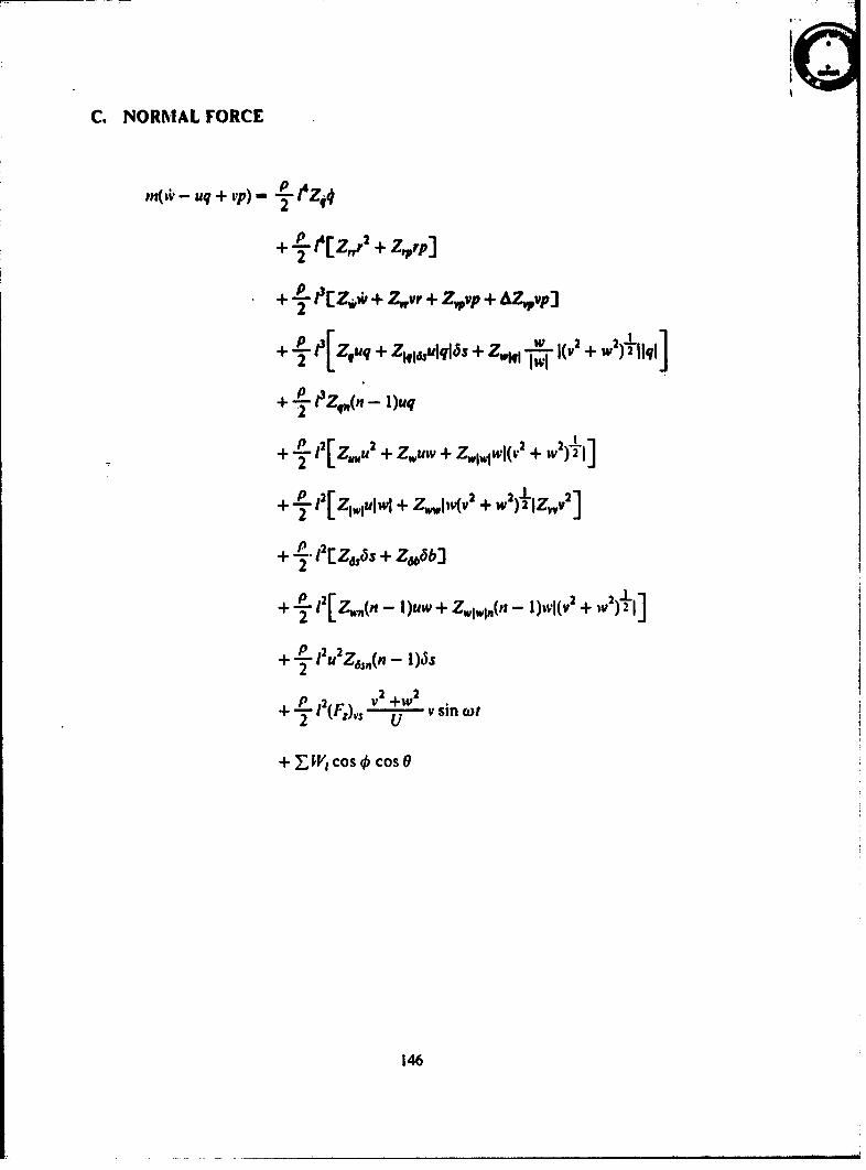
06~

C. NORMAL FORCE

n(tw- uq +vp)- p.~q

+ 4. 1'[Z,,r + Z,,rp]

2 e[Zi+Zvr+Z,,vp+A&Z~vpJ

+4.l2[Zi,,uq+Z,,Iaullv2 k +w2)I~vl2] F,1q

eA ,( - Iu

+ P~ l'[ZUR(I + Z)UW + - 1)IWI(V2 + W211 I

+4LP Z.12(F WP + W2 IVV + W2lC ) 12t.2

+2Wcs~cs

+ L- '[Z,,s +146b

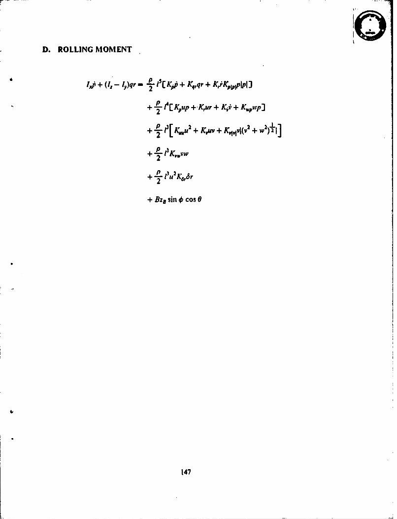
D. ROLLING MOMENT

1,f, + (! - ly)qr = Ko + Kqr + Ki+KWip)

+ K- + [ K,.u + K+# + K.,,,+p]

+ "P 13Kvw2 .

-+ l 3u 2 662 dr

+ Bzs sin 4 cos 0

147

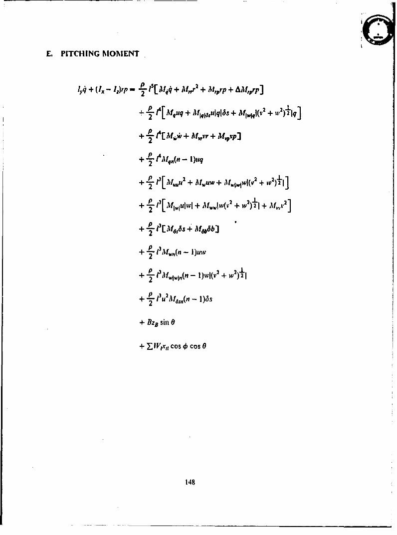
E. PITCHING MOMENT

~+ (IX-I,)rp 2 1$S[ llj4 +Milr2 + ilprp + AAi.,,rp]

+e"[Mqfuq + ilMtq13,lllq 6s + Atg~,I(v2 + w2)Iq]

+ ilf4w 4- Af~evr + ilfvpjp

+7L1e111qn( - 1)uq

+ 1 [I~,,ul+ Aluw + lMf.,. 1WI(v 2 + w 21,

+2.P[ 13 g~w +2 ~2~ + 2

2 [mIl si + 'If.luIu+w2 w~

P32

+1 U emIj,,(n - 1)I5s w2

+ BZB S'inO

+ I- ,v,V Co Cos

148

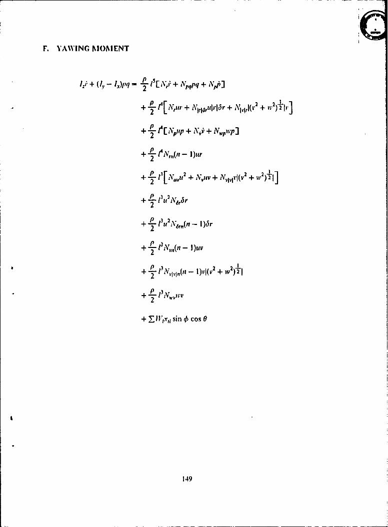
F. YAWING MOMENT

k- + QI, - I)pqm ~- IS[ lr + Nvpq q+ AJý

+-~ Ivir~~ + N ri~srulf-16Pr + N,,,j~rI 2 + I-

+ L e [ IPIIP + Alv, + A~P

+2Le~i - I)ur

[ y.,2+ V', +, IN71,11.I(V 2 1,+ w)

P2

+ j.2Ne,,n152

+ L I13, 2i 2/ 1o

1 49

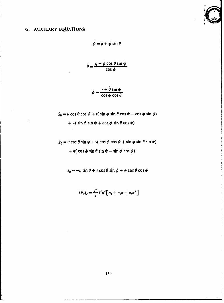
G. AUXILARY EQUATIONS

-p + sinO

q - • cos 0 sinCos

r + 0 sin f,cos 0 cos 0

o= u cos 0 cos 0, + v( sin 4, sin 0 cos 0, - cos 4 sin 0,)

+ w( sin 4 sin 4, + cos 4 sin 0 cos 4,)

= u cos 0 sin 0, + v( cos 4 cos 4, + sin 4 sin 0 sin 4,)

+ w( cos 4, sin 0 sin 4, - sin 4 cos 4,)

io = -u sin 0 + v cos 0 sin 4 + w cos 0 cos 4,

=P 12 u2[al + a2n + a3n 2 ]

150

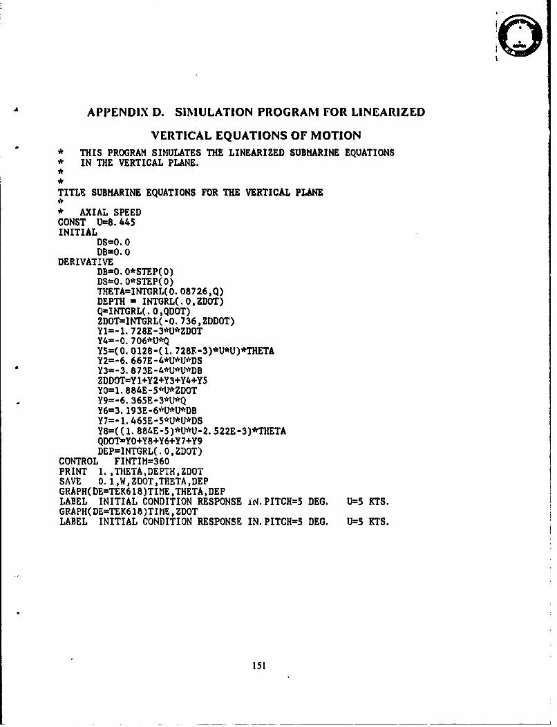
APPENDIX D. SIMULATION PROGRAM FOR LINEARIZED

VERTICAL EQUATIONS OF MOTION* THIS PROGRAM SIMULATES THE LINEARIZED SUBMARINE EQUATIONS* IN THE VERTICAL PLANE.

TITLE. SUBMARINE EQUATIONS FOR THE VERTICAL PLANE

* AXIAL SPEEDCONST U=8.445INITIAL

DS=O. 0DB0. 0

DERIVATIVEDB=O. 0*STEP(0)DS=0. 0*STEP(O)THETA=INTGRL(0. 08726 ,Q)DEPTH = INTGRL(.O,ZDOT)Q=INTGRL(. 0,QDOT)ZDOT=INTGRL( -0. 736, ZDDOT)Y1=-1. 728E-3*U*ZDOTY4=-0. 706*U*QY5=(0. 0128-(1. 728F.-3)*U*U)*THETAY2=-6. 667E-4*U*U*,DS

* Y3=-3. 873E-4*U*'U*DBZDDOT--Y +Y2+Y3+Y4+Y5Y0=1. 884E-5*U*ZDOTY9=-6. 365E-3*U*QY6=3.19 3E -6*U*U*DBY7=-1. 46SE-5*U*U*DSY8=( (1. 884E-5)*U*U-2. 522E-3)*THETAQDOT-YO+Y8+Y6+Y 7+Y9DEP=INTGRL(.0, ZDOT)

CONTROL FINTIM=36OPRINT 1. ,THETA,DEPTH,ZDOTSAVE 0. 1,W,ZDOT,TH[ETA,DEPGRAPH(DE=TEK618)TIME ,THETA ,DEPLABEL INITIAL CONDITION RESPONSE .u4.PITCH=5 DEG. U=5 KTS.GRAPH( DE=TEK6 18)TItIE ,ZDOTLABEL INITIAL CONDITION RESPONSE IN. PITCH=5 DEG. U=5 KTS.

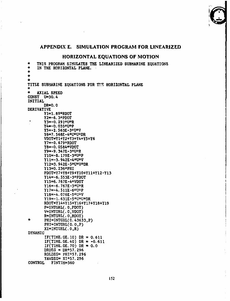
APPENDIX E. SIMULATION PROGRAM FOR LINEARIZED

HORIZONTAL EQUATIONS OF MIOTION* THIS PROGRAM SIMULATES THE LINEARIZED SUBMARINE EQUATIONS* IN THE HORIZONTAL PLANE.

TITLE SUBMARINE EQUATIONS FOR TKE HORIZONTAL PLANE

* AXIAL SPEEDCONST U=30.4INITIAL D=.

DERIVATIVEY1=1. 89*RDOTY2--6. 3*PDOTY3=-O. 291*U*RY4in-0. 035*U*PY5=-2. 563E-3*U*VY6=7. 568E-.4*U*U*DRVDOT-Y 1+Y2+Y3+Y4+Y5+Y6Y7=-O.679*RDOTY8=-0.0584*VDOTY9=-9. 347E-3*U*RY10=-8. 179E-3*U,*'PY11=-3. 942E-4*U*VY 12=3. 942E -5*Ul*U*'DRY13=0. 236*PHIPDOT-Y7+Y8+Y9+Y1O+Y1 1+Y12-Y13Y14=-6. 553E-3*PDOTY15=6. 767E-4*VDOTY16=-6. 767E-3*U*RY17=-4. 511E-6*U*PY18=-4. O76E-5*U*VY19=- 1. 63 1E-5*U*U*DRRDOT=Y14+Y 15+Y16+Y17+Y18+Y19P=INTGRL(. 0,PDOT)V=INTGRL(. O,VDOT)R=INTGRL(. O,RDOT)

* PHI=INTGRL(O. 43633,P)PHI=INTGRL(.0. ,P)

DNMCXI=INTGRL(. O)R)

IF(TIME. GE. 10) DR =0.611IF(TIME. GE. 40) DR = -0.611IF(TIME.GE. 70) DR - 0.0DRDEG = DR*57. 296RQLDEG= PHI*57. 296YAWDEG= XI*57. 296

CONTROL FINTI!1=360

152

PRINT 1. ,V,YAWDEG,ROLDEGSAVE 0. 1,V,YAWDEGROLDEG,DRDEGGRAPH(DE=TEv618)TIME ,YAWDEG,ROLDEGLABEL FORCED RESPONSE TO 35 DEG. RUDDER U=18 KTS.

153

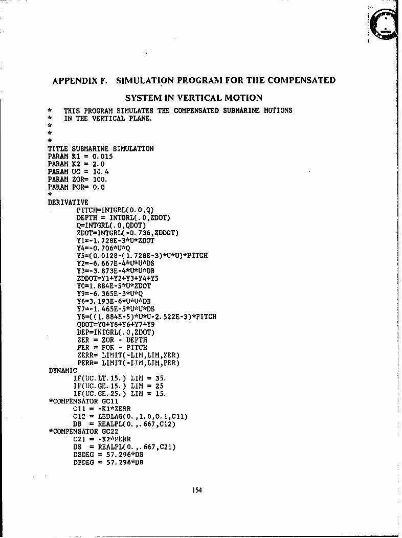
APPENDIX F. SIMULATION PROGRAM FOR THE COMPENSATED

SYSTEM IN VERTICAL MOTION* THIS PROGRAM SIMULATES THE COMPENSATED SUBMARINE MOTIONS* IN THE VERTICAL PLANE.

TITLE SUBMARINE SIMULATIONPARAM Kl = 0.015PARAM K2 = 2. 0PARAM UC = 10. 4PARAM ZOR= 100.PARAM POR= 0. 0

DERIVATIVEPITCH=INTGRL(0. OQ)DEPTH = INTGRL(.0,ZDOT)Q=INTGRL(. 0,QDOT)ZDOT=-INTGRL( -0. 736,ZDDOT)Yl=-1. 728E-3*U*ZDOTY4=-O. 706*U*QY5=(O. 0128-Cl. 728E-3)*U*U)*PITCHY2=-6. 667E-4*U*U*DSY3=-3. 873E-4*U*U*DBZDDOT=-Y +Y2+Y3+Y4+Y5Y0=1. 884E-5*U*ZDOTY9=-6. 365E-3*U*QY6=3. 19 3E -6*U*U'UDBY7=-1. 465E-5*U*U*DSY8=( (1. 884E-5)*U*U-2. 522E-3)*PITCHQDOT-YO+Y8+Y6+Y7+Y9DEP=INTGRL(.0, ZDOT)ZER = ZOR - DEPTHPER = POR - PITCH{ZERR= LIMIT( -LIM, LIM, ZER)PERR= LIMIT( -LIM,LIM,PER)

DYNAMICIF(UC. LT. 15.) LIII = 35.IF(UC. GE. 15.) LIMI = 25IF(UC. GE. 25.) LIM m15.

*COM.PENSATOR GC 11Cll = -Kl*ZERRC 121 = LEDLAG(O. ,1. 0, 0.1,C 11)DB = REALPL(O. .667,C12)

*COMPENSATOR GC22C21 = -K2*PERRDS = REALPL(O.,.667,C21)DSDEG = 57. 296'*DSDEDEG = 57. 296*DB

154

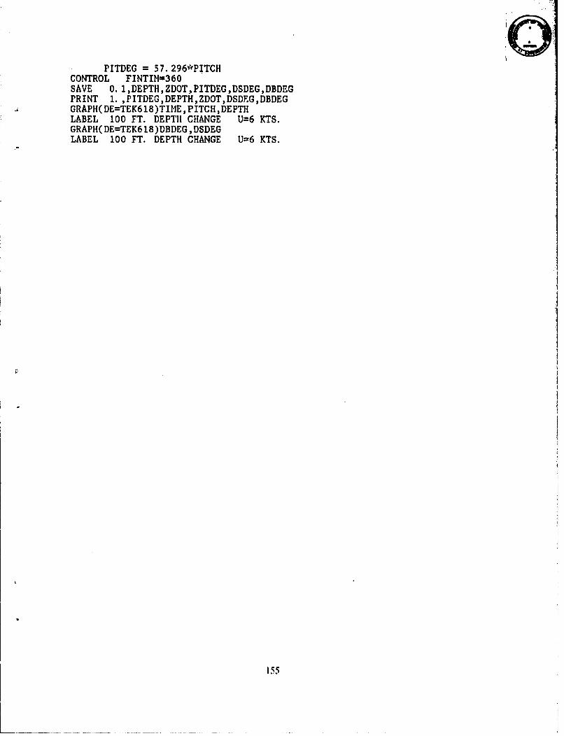
PITDEG =57. 296*PITCHCONTROL FINTIM=36OSAVE 0. 1,DEPTH,ZDOT,PITDEG,DSDEG,DBDEGPRINT 1. ,PITDEG,DEPTH,ZDOTDSDEG,DBDEGGRAPH(DE=TEK618)TIIIEPITCHDEPTHLABEL 100 FT. DEPTH CHANGE U=6 KTS.GRAPHI(DE=TEK618)DBDEG ,DSDEGLABEL 100 FT. DEPTH CHANGE U=6 KTS.

1 55

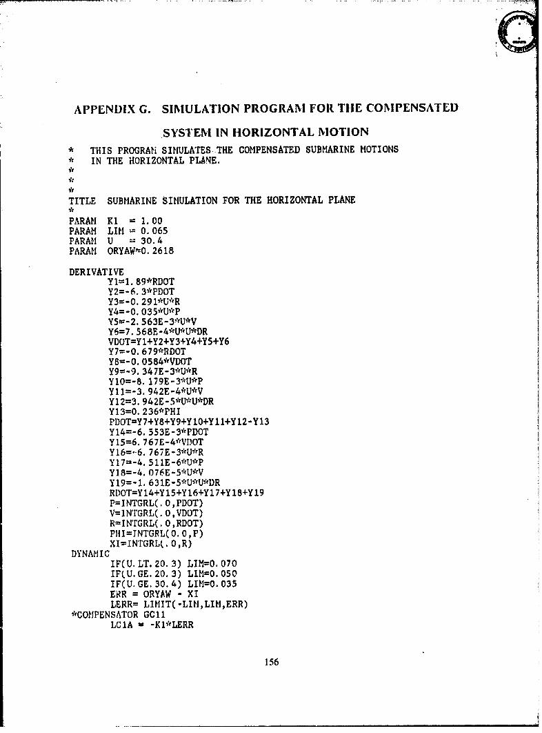
APPENDIX G. SIMULATION PROGRAM FOR THE COMPENSATED

.SYSTEMI IN HORIZONTAL NIOTION* THIS PROGRAH SIMULATES THE COMPENSATED SUBMARINE MOTIONS* IN THE HORIZONTAL PLANE.

TITLE SUBMARINE SIMULATION FOR THE HORIZONTAL PLANE

PARAM Ki 1.00PARAM LIM 0. 065PARAM U -30.4PARAM ORYAW=0. 2618

DERIVATIVEY1=1. 89*RDOTY2=-6. 3'PDOTY3=-O.291*U*RY4=-O. O35'*U*PY5=-2. 563E-3*U*VY6=7. 568E-4*U*U*DRVDOT=Y +Y2+Y3+Y4+Y5+Y6Y7=-O. 679*RDOTY8=-O. o584*'VDOTY9=-9. 347E-3*U*'RY10=-8. 179E-3*U*~PY11=-3. 942E-4?rU*VY12=3. 942E-5*U~rU*DRY13=0. 236*PHIPDOT=Y7+Y8+Y9+YlO+Y1 1+Y12-Y13Y14=-6. 553E-3*PDOTY15=6. 767E-4*VDOTY16=-6. 767E-3*U*~RY17=-4. 511E-6*'U*PY18=-4. 076E-5*U*VY19=-1.63E **UDRDOT=Y14+YlS+Y16+Y1 7+Y18+Y19P=INTGRL(. O,PDOT)V=IN'rGRL(. O,VDOT)R=INTrGRL(. 0,RDOT)PHI=INTGRL(0. 0, P)XI=INTGRL(. 0,R)

DYNAMICIF(U. LT. 20. 3) LIM=O. 070IF(U. GE. 20. 3) LI&O. 050IF(U. GE. 30. 4) LIM=0. 035ERR = ORYAW - XILERR= LIMIT( -LIII,LIM,ERR)

*COM~PENSATOR GC 11LCIA = -KPl'LERR

156

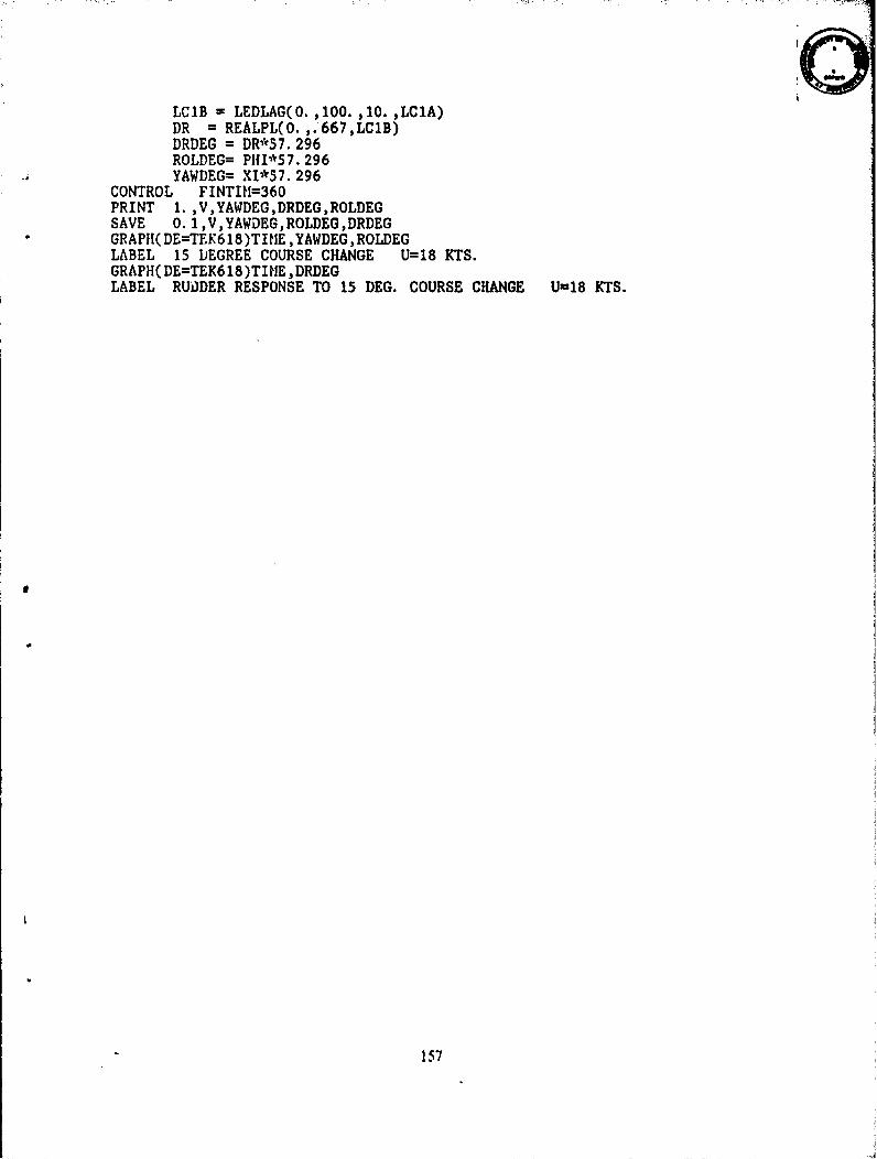
L~lB =LEDLAG(O. .100. ,1O. ,LClA)DR =REALPL(O. ,.667,LC1B)DRDEG = DR*57. 296ROLDEG= PHII'57. 296YAWDEG= XI*57. 296

CONTROL FINTIfl=36OPRINT 1. ,V,YAWDEG,DRDEG,ROLDEGSAVE 0. 1,V,YAWDEG,ROLDEG,DRDEGGRAPII(DE=TEK618)TIIE ,YAWDEG,ROLDEGLABEL 15 DJEGREE COURSE CHANGE U=18 KTS.GRAPH( DE=TEK6 18 )TIME,*DRDEGLABEL RUD)DER RESPONSE TO 15 DEG. COURSE CHANGE U=18 KTS.

157

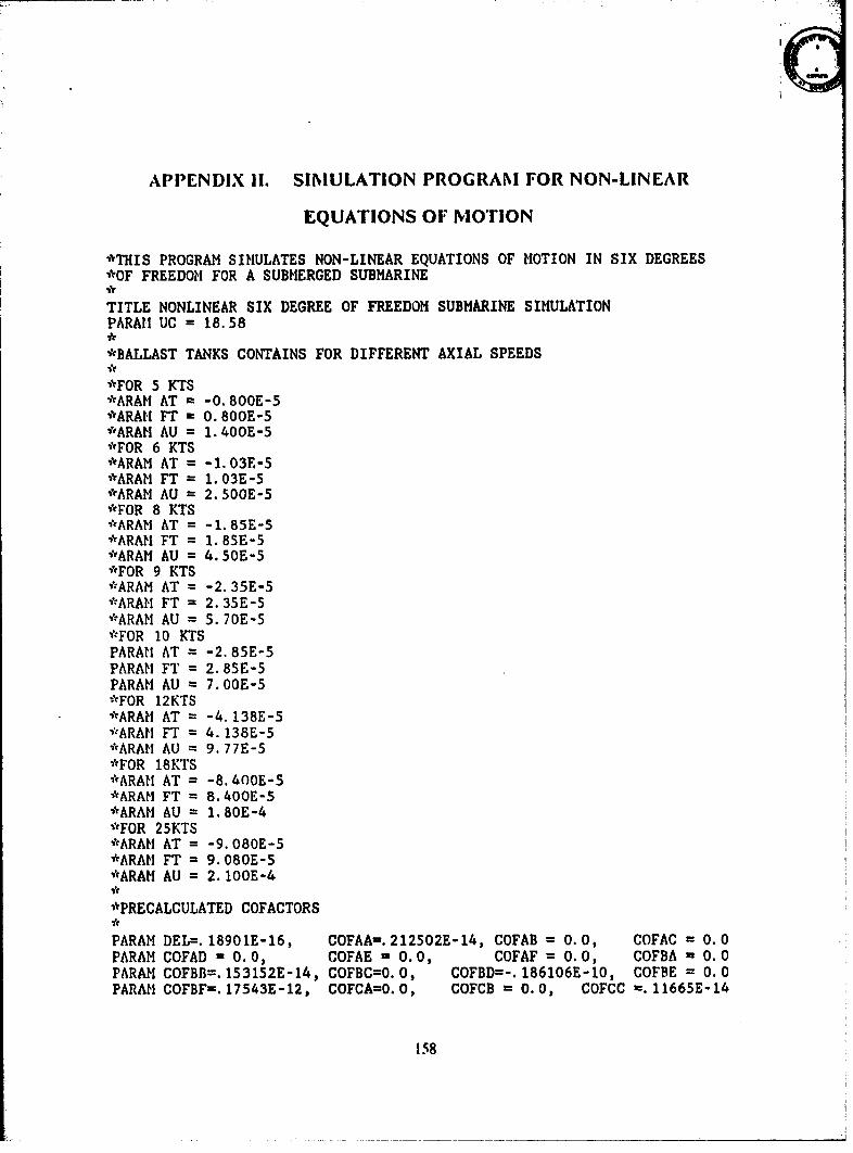
APPENDIX II. SIMULATION PROGRAM FOR NON-LINEAR

EQUATIONS OF MOTION

*THIS PROGRAM SIMULATES NON-LINEAR EQUATIONS OF MOTION IN SIX DEGREES*OF FREEDOM FOR A SUBMERGED SUBMARINE

TITLE NONLINEAR SIX DEGREE OF FREEDOM SUBMARINE SIMULATIONPARAI UC = 18.58*

*BALLAST TANKS CONTAINS FOR DIFFERENT AXIAL SPEEDS**FOR 5 KTS*ARAM AT = -0.800E-5*ARAH FT = 0.800E-5*ARAM AU = 1.400E-5*FOR 6 KTS*ARAM AT = -1.03E-5*ARAM FT = 1.03E-5*ARAM AU = 2.500E-5"*FOR 8 KTS*ARAM AT = -1. 85E-5*ARAH FT = 1.85E-5*ARAM AU = 4.50E-5"*FOR 9 KTS*ARAM AT = -2.35E-5*ARAM FT = 2.35E-5*ARAM AU = 5.70E-5*FOR 10 KTSPARAH AT = -2.85E-5PARAM FT = 2.85E-5PARAM AU = 7.OOE-5*FOR 12KTS*ARAM AT = -4. 138E-5*ARAM FT = 4. 138E-5*ARAM AU = 9.77E-5*FOR 18KTS*cARAM AT = -8.400E-5*ARAM FT = 8.400E-5*ARAM AU = 1.80E-4*FOR 25KTS*ARAM AT = -9.080E-5*ARAM FT = 9.080E-5*ARAM AU = 2. 100E-4

*PRECALCULATED COFACTORS

PARAM DEL=. 18901E-16, COFAA=. 212502E-14, COFAB = 0.0, COFAC = 0. 0PARAM COFAD = 0.0, COFAE = 0.0, COFAF = 0.0, COFBA = 0.0PARAM COFBB=.153152E-14, COFBC=O.0, COFBD=-. 186106E-10, COFBE = 0.0PARAM COFBF=.17543E-12, COFCA=0.O, COFCB = 0.0, COFCC =.11665E-14

158

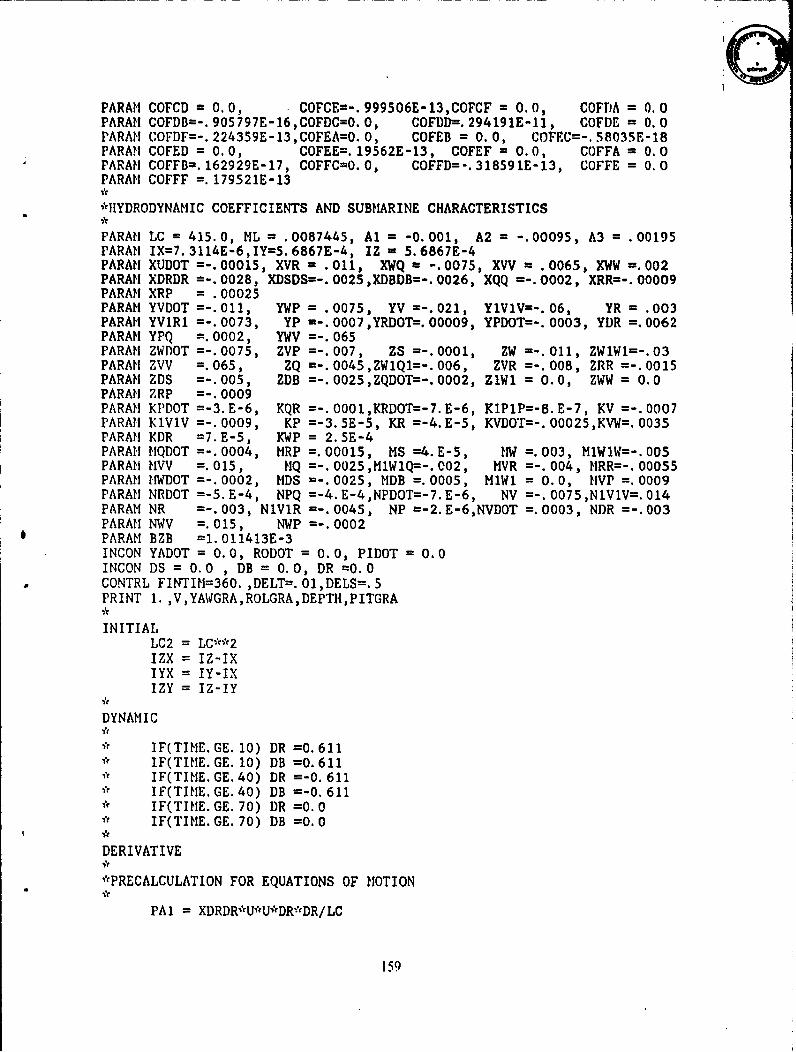
FARAH COFCD = 0.0, COFCE=-. 999506E-13,COFCF =0.0, COFIJA = 0.0FARAH COFDB=-.905797E-16,COFDC=0.0, COFDD=.294191E-11, COFDE = 0.0PARAH COFDF=-.224359E-13,COFEA=0.O, COFEB = 0.0, COFEC=-.58035E-18PARAM COFED = 0.0, COFEE=.19562E-13, COFEF = 0.0, COFFA = 0.0PARAM COFFB=.162929E-17, COFFCO0.0, COFFD=-.318591E-13, COFFE = 0.0PARAH COFFF =. 179521E-13

*HIYDRODYNAMIC COEFFICIENTS AND SUBMARINE CHARACTERISTICS

PARAM LC = 415.0, ML = .0087445, Al = -0.001, A2 = -.00095, A3 = .00195FARAH IX=7.3114E-6,IY=5.6867E-4, IZ = 5.6867E-4FARAH XUDOT =-. 00015, XVR = .011, XWQ = -.0075, XVV = .0065, XWW =.002FARAH XDRDR =-. 0028, XDSDS=-. 0025 ,XDBDB=-. 0026, XQQ -. 0002, XRR=-. 00009PARAM XRP = . 00025FARAH! YVDOT =-.011, YWP = .0075, YV =-.021, Y1V1V=-. 06, YR = .003PARAI' YV1R1 =-. 0073, YP =-. 0007,YRDOT=. 00009, YPDOT=-. 0003, YIJR =.0062PARAM YPQ =.0002, WV =-. 065PARAM' ZWDOT =-. 0075, ZVP =-. 007, ZS =-. 0001, ZW =-. 011, ZW1W1=-.03PARAM ZVV =.065, ZQ =-. 0045,ZW1Q1=-. 006, ZVR =-. 008, ZRR =-. 0015PARAM ZDS =-. 005, ZDB =-. 0025,ZQDOT=-.0002, ZiWi = 0.0, ZWW = 0.0FARAH ZRP =-. 0009PARAM' KPDOT =-3.E-6, KQR =-. 0001,KRDOT=-7.E-6, KlP1P=-8.E-7, KV =-. 0007PARAII K1VlV =-. 0009, KP =-3.5E-5, KR =-4.E-5, KVDQT=-. 00025,KVW=. 0035PARAM KDR =7.E-5, KWP = 2.5E-4PARAM HQDOT =-.0004, MRP =.00015, MS =4.E-5, MW =.003, MlIWW=-. 005PARAM MVW =.015, mQ =-. 0025,M1W1Q=-. 002, MVR =-. 004, HRR=-. 00055PARAM IIWDOT =-.0002, MDS =-. 0025, MDB =.0005, lM1W1 = 0.0, mVP, =.000PARAM' NRDOT =-5.E-4, NPQ =-4.E-4,NPDOT=-7.E-6, NV =-. 0075,NIV1V=.014PARAtI NR =-.003, NiViR =-.0045, NP =-2.E-6,NVDOT =.0003, NDR =-.003FARAM NWV =.015, NWP =-. 0002

*PARAM BZB =1.011413E-3INCON YADOT = 0.0, RODOT = 0.0, PIDOT =0.0INCON DS = 0.0 , DB = 0.0, DR =0.0

* ~CONTRL FINTIM=360. ,DELT=.01,DELS=.5PRINT 1. ,V ,YAWiGRA ,ROLGRA ,DEPTH,PITGRA

INITIAL

LC2 = LC**2

DYNAMIC

IF(TIME. GE. 10) DR =0.611IF(TIME. GE. 10) DB =0.611IF(TIME. GE. 40) DR =-0. 611If(TIME. GE. 40) DB =-0. 611IF(TIME. GE. 70) DR =0. 0IF(TIME.GE. 70) DB =0. 0

DERIVATIVE

*ePRECALCULATI0N FOR EQUATIONS OF MOTION

PAl = XDRDR*U*U*DR*DR/LC

159

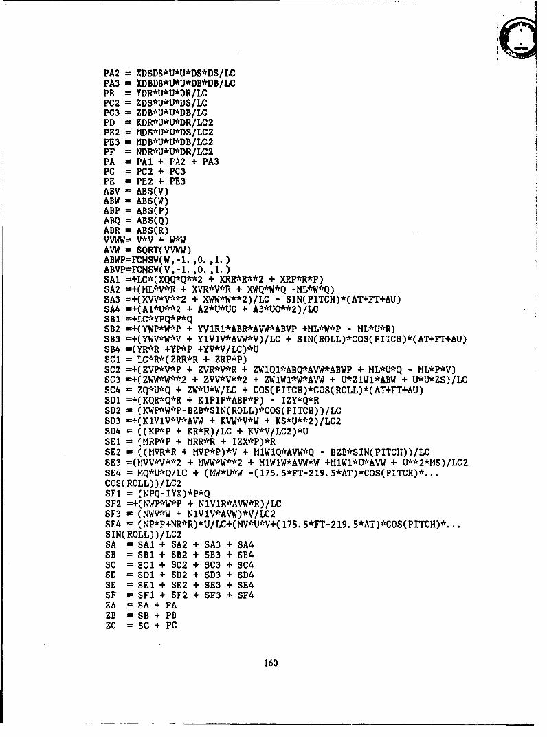
PA2 = XDSDS*U'vU*DS*DS/LCPA3 = XDBDB*U*U*DB*DB/LCPB = YDR*U*U*DR/LCPC2 = ZDS*U*U*DS/LCPC3 = ZDB*U*U*DB/LCPD = KDR*U*U*DR/LC2PE2 = HDS*4J*U*DS/LC2PE3 = MDB*U*U*DB/LC2PF = NDR*U*U*DR/LC2PA = PAl + PA2 + PA3PC = PC2 + PC3PE = PE2 + PE3ABV = ABS(VABW = ABS(W)ABP = ABS(P)ABQ = ABS(Q)ABR = ABS(R)vvwW= VA-v + ViewAVW = SQRT( VVWW)ABWP=FCNSW(W, -1. ,0. 1.)ABVP=FCNSW(V,-l. 10. 1.)SAl =+LC*(XQQ*Q**2 + XRR*R**2 + XRP*R*P)SA2 =+(KL*,V*R + XVR*V*R + XI4Q*W*Q -I1L*W*Q)SA3 =+(XVV*V**2 + XWW*W**2)/LC - SIN(PITCH)*(AT+FT+AU)SA4 =+(A1*U*c*2 + A2*t1*UC + A3*UC**2)/LCSB 1 =+LCecYPQ*P*Q582 =+(YWP*W*P + YVlRl*ABR*AVWvABVP +ML*W*P - ML*U*R)SB3 =+(YWV*W*V + YlV1V*AW*VV)/LC + SIN(ROLL)*COS( PITCH)*(AT+FT+AU)SB4 =(YR*R +YP*P +YV*V/LC)*USC1 = LC*R*(ZRR*R + ZRP*P)5C2 =+( ZVP*V*P + ZVR*V*R + ZW1Q1*ABQ*AVW*ABWP + IILvU*Q - ML*P*V)SC3 =+(ZWW*W**2 + ZVV*V**2 + ZW1Wl*W*AVW + U*ZlW1*ABW + U*U*ZS)/LCSC4 = ZQ*U*Q + ZW*U*W/LC + COS(PITCH)*COS(ROLL)*(AT+FT+AU)SD1 =+(KQR*Q*R + KlP1P*ABP*P) - IZY*Q*RSD2 = (KWP*W*~P-BZB*SIN(ROLL)*COS(PITCH) )/LCSD3 =+(KlV1V*V*AVW + KVW*V*W + KS*U**2)/LC2SD4 = ((KP*P + KR*R)/LC + KV*V/LC2)*USE1 = (MRP*!P + MRR*R + IZX*P)*eRSE2 =((MVR*R + KVP*P)*V + !11W1Q*AVW*Q - BZB*SIN(PITCII))/LCSE3 =(M~VV*V**2 + IIWW*W**2 + HlWlW*~AW*W +ItlWl*U*AVW + U**2*?MS) /LC2SE4 = MQ*U*Q/LC + (MW*U*W -(175.5*FT.219.5*AT)*COS(PITCH)*...COS( ROLL) )/LC2SF1 = (NPQ-IYX)*P*QSF2 =+( NlP*'W*~P + N 1V R*AVW*R) /LCSF3 = (NWV'*W + N1VlV*AVW)*V/LC2SF4 = (NP*cP+NR*rR)*U/LC+(NV*U*V+( 175. 5*FT-219. 5*AT)*COS(PITCII)*...SIN(ROLL))/LC2SA = SAl + SA2 + SA3 + SA4SB = B1 + B2 +SB3 +SB4SC = C1+ SC2 +SC3 + C4SD = SD1 + SD2 + SD3 + SD4SE - SEl + SE2 + SE3 + SE4SF = SF1 + SF2 + SF3 + SF4ZA = SA + PAZB =SB +PBZC = SC +PC

160

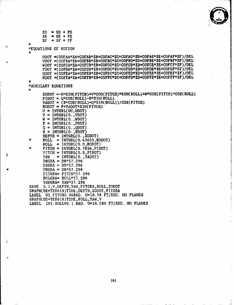
ZD - SD + PDZE = SE + PEZF = SF + PF

*EQUATIONS OF MOTION

UDOT -(COFAA*ZA+COFAB*ZB+COFAC*ZC+COFAD*ZD+COFAE*ZE+COFAF*ZF) /DEIafk VDOT =(COFBA*ZA+COFBB*ZB+COFBC*ZC+COFBD*ZD+COFBE*ZE+COFBF,*ZF) /DEL

WDOT =(COFCA*%ZA+COFCB*ZB+COFCC*ZC+ COFCD*ZD+COFCE*ZE+COFCF*ZF) /DELPDQT =(COFDA*ZA+COFDB*ZB+COFDC*ZC+COFDD*VZD+COFDE*ZE+COFDF*vZF) fUELQDOT =( COFEA*ZA+COFEB*ZB+COFEC*ZC+COFED*ZD+COFEE*ZE+COFEF*~ZF) /DEI.RDOT =( COFFA*ZA+COFFB*ZB+COFFC*ZC+COFFD*'ZD+COFFE*ZE+COFFF*ZF) /DEL

*AUXILARY EQUATIONS

ZODOT =-U*SIN( PITCH)+V*COS( PITCII)*SIN( ROLL)+W*COS( PITCII),*CCOS(ROLL)PIDOT = Q*COS(ROLL)-R*SIN(ROLL)MAOT = (R*COS(ROLL)+Q*SIN(ROLL) )/COS(PITCH)RODOT = P+YADOT,*SIN(PITCH)U = INTGRL(UC,UDOT)V = INTGRL(O. ,VDOT)W = INTGRL(O. ,WDOT)P = INTGRL(O. ,PDOT)Q = INTGRI.(O. ,QDOT)R = INTGRL(O. ,RDOT)DEPTH = INTGRL(O. ,ZODOT)

* ROLL = INTGRL(O.43633,RODOT)ROLL = INTGRL(O.O,RODOT)

* PITCH = INTGRL(O. 7854,PIDOT)PITCH = INTGRL(O.O,PIDOT)YAW = INTGRL(O. ,YADOT)DBGRA = DB*57. 296DSGRA = DS*57. 296DRGRA = DR*57. 296PITGRA= PITCH*57. 296ROLGRA= ROLL*57. 296YAWGRA= YAW*57. 296

SAVE 0. 1,V,DEPTIIYAWi,PITGRA,ROLL,ZODOTGRAPH(DE=TEK618)TINIE DEPTH, ZODOT,PITGRALABEL NI.PITCIIQ.O4RAD. U=18.58 FT/SEC. NO PLANESGRArH(DE=TEK618)TIIE ,ROLL,YAW,VLABEL INI.ROLL-O.1 RAD. U=18.580 FT/SEC. NO PLANES

161

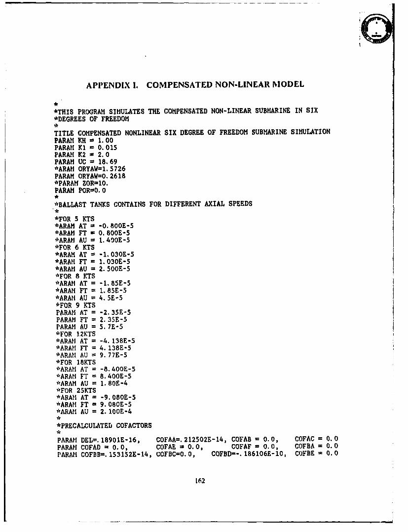
APPENDIX 1. COMPENSATED NON-LINEAR MODEL

*THIS PROGRAM SIMULATES THE COMPENSATED NON-LINEAR SUBMARINE IN SIX*DEGREES OF FREEDOM

TITLE COMPENSATED NONLINEAR SIX DEGREE OF FREEDOM SUBMARINE SIMULATIONPARAM KH = 1.00PARAM Ki = 0.015PARAM K2 = 2.0PARAM UC = 18.69*ARAM ORYAW=1. 5726PARAM ORYAW=O. 2618*PARAM ZOR1O.PARAM POR=O. 0

,,*BALLAST TANKS CONTAINS FOR DIFFERENT AXIAL SPEEDS

*FOR 5 KTS*ARAM AT = -0. 800E-5*ARAM FT = 0.800E-5*ARAM AU = 1.400E-5*FOR 6 KTS*ARAM AT = -1. 030E-5*ARAM! FT = 1. 030E-5*ARAM AU = 2.500E-5*FOR 8 KTS*ARAM AT = -1. 85E-5*ARAM FT = 1.85E-5*ARAM! AU = 4.5E-5*FOR 9 KTSPARAM AT = -2.35E-5PARAM FT = 2.35E-5PARAI! AU = 5.7E-5*FOR 12KTS*ARAM! AT = -4. 138E-5*ARAI FT = 4. 138E-5*ARAM1 AU = 9.77E-5*FOR 18KTS"*ARAM AT = -8. 400E-5*ARAM FT = 8.400E-5*ARAM AU = 1.80E-4*FOR 25KTS*ARAM! AT = -9. 080E-5*ARAMi FT = 9. 080E-5*ARAM1 AU = 2. 100E-4

*PRECALCULATED COFACTORS

PARAM DEL=.18901E-16, COFAA--.212502E-14, COFAB = 0.0, COFAC = 0.0PARAM COFAD = 0.0, COFAE = 0.0, COFAF = 0.0, COFBA = 0.0PARAM COFBB=.153152E-14, COFBC=0.0, COFBD=-.186106E-10, COFBE = 0.0

162

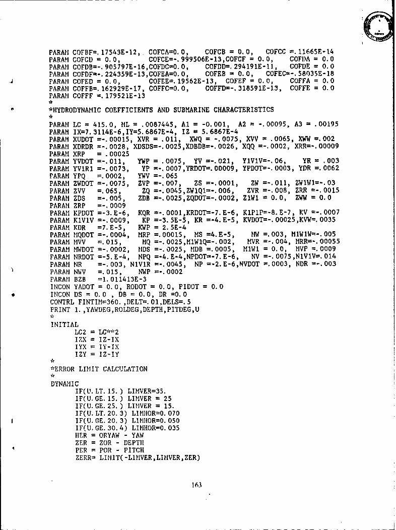
PARAH COFBF=.17543E-12,. COFCA=0.0, COFCB = 0.0, COFCC =.11665E-14FARAM COFCD = 0.0, COFCE=-.999506E-13,COFCF = 0.0, COFI)A = 0.0PARAII COrDI3-.905797E-16,COFDCO0.0, COFDD=.294191E-11, COFUE = 0.0PARAM COFDF=-. 224359E-13,COFEAO0.0, COFEB = 0.0, COFEC=-.58035E-18FARAM COPED = 0.0, COFEE=.19562E-13, COFEF = 0.0, COFFA = 0.0PARAM COFFB=.162929E-17, COFFC=0.0, COFFD=-.318591E-13, COFFE = 0.0PARAN COFFF =.179521E-13

*HYDRODYNAM1IC COEFFICIENTS AND SUBMARINE CHARACTERISTICS

PARAM LC = 415.0, ML = .0087445, Al = -0.001, A2 = -.00095, A3 = .00195PARAM IX=7.3114E-6,IY=5.6867E-4, IZ = 5.6867E-4PARAM XUDOT =-. 00015, XVR = .011, XWQ = -.0075, XVV = .0065, XWW =.002PARAH XDRDR =-. 0028, XDSDS=-. 0025,XDBDB=-. 0026, XQQ =-. 0002, XRR=-. 00009PARAM XRP = .00025PARAM YVDOT =-. 011, YWP = .0075, YV =-.021, YlVlV=-.06, YR = .003PARAM YVlRl =-. 0073, YP =-. 0007,YRDOT-. 00009, YPDOT--. 0003, YDR =.0062PARAM YPQ =.0002, YWV =-.065PARAM ZWDOT =-. 0075, ZVP =-.007, ZS =-. 0001, ZW =-.011, ZWlW1=-.03PARAM ZVV =.065, ZQ =-. 0045,ZWlQl=-. 006, ZVR =-.008, ZRR =-. 0015PARAM ZDS =-.005, ZDB =-.0025,ZQDOT=-.0002, ZiWi = 0.0, ZWW = 0.0PARAM ZRP =-. 0009PARAM KPDOT =-3.E-6, KQR =-. 0001,KRDOT=-7.E-6, K'1FIP=-8.E-7, RV =-.0007PARAM K1V1V =-. 0009, KP =-3..5E-5, KR =-4.E-5, KVDOT=--. 00025,KVW=. 0035PARAM KDR =7.E-5, KWP = 2.5E-4PARAM HQDOT =-. 0004, MRP =.00015, MS =4.E-5, MW =.003, M1WlW=-. 005PARAM MVV =.015, NQ =-. 0025,MlW1Q=-. 002, MVR =-.004, MRR=-. 00055PARAH MWDOT =-.0002, lIDS =-. 0025, MDB =.0005, MlWi = 0.0, HVP =.0009FARAM NRDOT =-S.E-4, NPQ =-4.E-4,NPDOT=-7.E-6, NV =-. 0075,N1V1V=.014FARM! NR =-. 003, NiViR =-. 0045, NP =-2.E-6,NVDOT =.0003, NDR =-.003FARAM NWV =. 015, NWP =-. 0002PARAII BZB =1.011413E-3INCON YADOT = 0.0, RODOT = 0.0, PIDOT =0.0INCON DS = 0.0 , DB = 0.0, DR =0.0CONTRL, FINTIM=360. ,DELT=. 01,DELS=.5PRINT 1. ,YAWDEG,ROLDEG,DEPTH,PITDEG,U

INITIALLC2 = LC**2IZX =IZ-IXIYX = Y-IXIZY =IZ-IY

*ERROR LIMIT CALCULATION

DYNAMICIF(I. LT. 15.) LIMVER=35.IF(U. GE. 15. ) LIMVER =25IF(U.GE. 25.) LIIIVER = 15.IF(U. LT. 20. 3) LIMHORO0. 070IF(U. GE. 20. 3) LI1NHOR=0. 050IF(U. GE. 30. 4) LIMIIOR=0. 035HER = ORYAW - YAWZER = ZOR - DEPTHPER = FOR - PITCHZERR= LIHIT( -LlNVER,LIMVER,ZER)

163

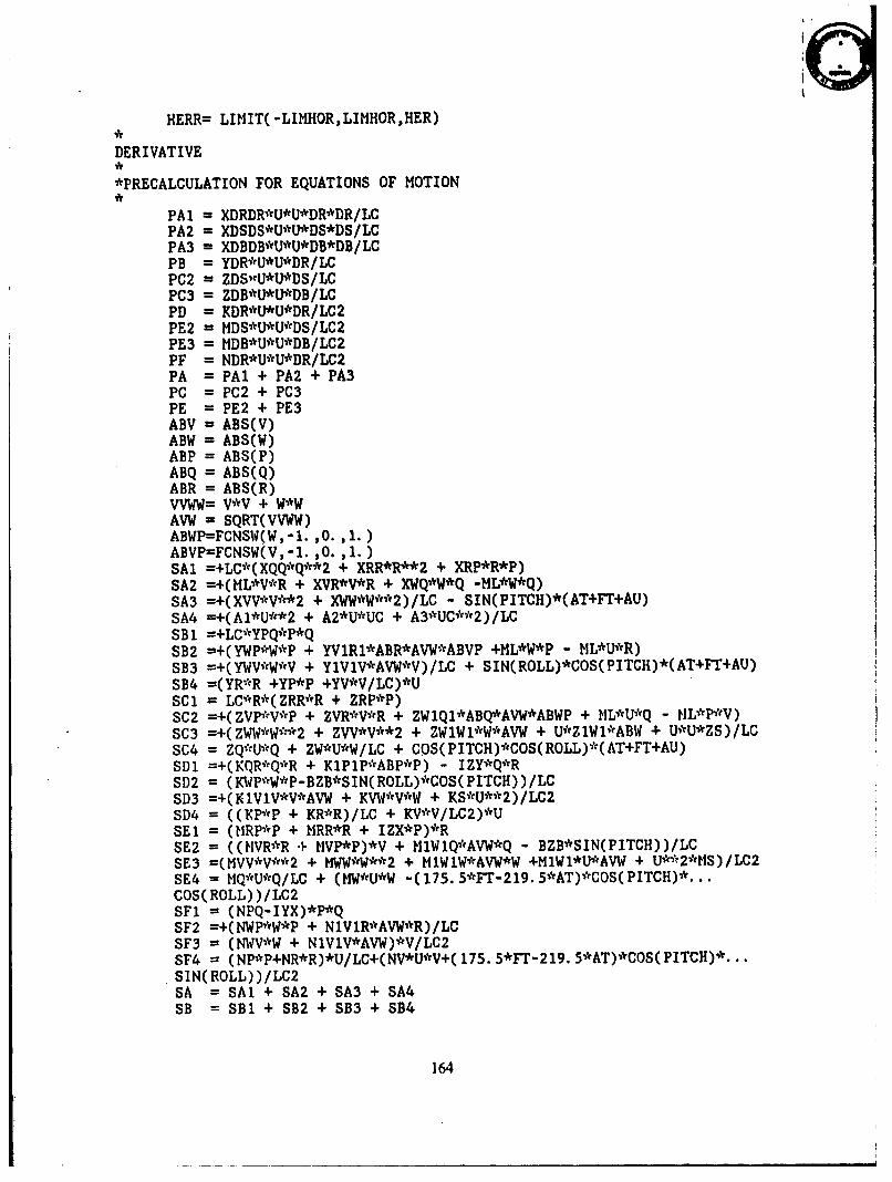
H'ERR= LIlIIT( -LIMHOR,LIMHOR,HER)

DERIVATIVE

*PRECALCULATION FOR EQUATIONS OF MIOTION

PAl = XDRDR*U*U*DR*DR/LCPA2 m XDSDS*U*U*DS*DS/LCPA3 = XDBDB*U*U*DB*DB/LCPB = YDR*U*U*DR/LCPC2 = ZDSwUI*U*DS/LCPC3 = ZDB*U*U*DB/LCPD = KDR*U*U*DR/LC2PE2 = MDS*U*U*DS/LC2PE3 = MDB*U*U*DB/LC2PF = NDR*U*U*DR/LC2PA = PAl + PA2 + PA3PC = PC2 + PC3PE =PE2 + PE3ABV = ABS(V)ABW = ABS(W)ABP = ABS(P)ABQ = ABS(Q)ABR = ABS(R)VVWW= V*V + W*W

AV`W = SQRT(VVWW)ABWP=FCNSW(W,-l.,O.,1.)ABVP=FCNSW(V,-1.,O. 1.)SAl =+LC*(XQQ*Q**2 + XRR*R**2 + XRP*R*P)SA2 =+(KL*V*R + XVR*V*R, + XW~Q*W*Q -ML*W*Q)SA3 =+(XVV*V**2 + X(14I*W**2)/LC - SIN(PITCH)*(AT+FT+AU)SA4 =+(Al*U**2 + A2*U*UC + A3*UC**2)/LCSB 1 =+LC*YPQ*P*QSB2 =+( 'W'I*W*P + YV1R1*ABR*AVW*ABVP +ML*W*P - ML*U*R)SB3 =+(YWV*W*V + YlV1V*AVW*V)/LC + SIN(ROLL)*COS(PITCII)*(AT+FT+AU)SB4 =(YR*R +YP*P +YV*V/LC)*USC1 = LC*R*(ZRR*R + ZRP*P)SC2 =+( ZVP*V*P + ZVR*VtVR + ZW1Q1*ABQ*AVW*ABWP + ML*U*Q - ML*P*eV)SC3 =+( ZWW*W**2 + ZVV*V**2 + ZW1W1*W*AVW + U'*ZlW1*ABWi + U*U*ZS)/LCSC4 = ZQ*U'*Q + ZW*U*W/LC + COS(PITCH)*COSCROLL)*(AT+FT+AU)SD1 =+(KQR*Q*R + K1P1P*ABP*P) - IZY*Q*RSD2 = (KWP*W*P-BZB*SIN(ROLL)*COS(PITCH))/LCSD3 =+(K1VlV*V*AVW + KVW*V*W + KS*U**2)/LC2SD4 = ((1KP*P + KR*R)/LC + KV*V/LC2)*USE1 = (IIRP*P + MRR*R + IZX*P)*RSE2 =((MVR*R + MVP*P)*V + M1WlQ*AVW*Q - BZB*SIN(PITCH))/LCSE3 =(MVV*V**~2 + HWW*W**2 + IMlW1W*AVW*W +M1Wl*U*AVW + U**2*HS)/LC2SE4 = MQ*U*Q/LC + (IIW*U*W -(175.5*FT-219.5*AT)*COS(PITCH)*...COSC ROLL) )/LC2SF1 = (NPQ-IYX)*P*QSF2 =+(NWP*W*P + NlVlR*AVW*R)/LCSF3 = (NWV*W + N1VlV*AVW)*V/LC2SF4 =CNP*P+NR*R)*U/LC+(NV*U*V+( 175. 5*FT-2 19. 5*AT)*COS( PITCH)*..

SA =SAl + SA2 + SA3 + SA4SB =SBl + SB2 + SB3 + SB4

164

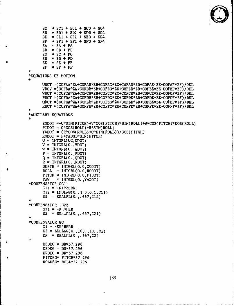
SC = SC1 + SC? + SC3 + SC4SD - SDI + SD2 + SD3 + 504SE =SEl + SE2 + SE3 + SE4SF - SF1 + SF2 + SF3 + SF4ZA =5A +PAZB = SB +PBZC = SC + PCZD = SD + PDZE = SE + PEZF = SF + PF

*EQUATIONS OF MOTION

* DT=CFAZ+OA*BCFC*CCFDVDCFEZ+OA*F/E

UDOT =( COFBAAZA+COFAB*ZB+COFAC,*ZC+COFAD*ZD+COFAE*ZE+COFAF*ZF) /DELVDO" =7( COFBA*ZA+COFBB*ZB+COFBCCZC+COFCD*'ZD+COFCE*ZE+COFCF*ZF) /DELWDOT =( COFDA*ZA+COFDB*ZB+COFDC*ZC+COFCD*ZD+COFDE*ZE+COFCF*rZF) /DELQDOT =( COFEA*ZA+COFEB*ZB+COFEC*ZC+COFED*ZD+COFEE*ZE+COFEF,*ZF) /DELRDOT m( COFFA*ZA+COFFB*ZB+COFFC*ZC+COFFD*ZD+COFFE*ZE+COFFF*ZF) /DEL

*AUXI LARY EQUATIONS

ZODOT =-U*SINC PITCH)+V*COS( PITCH)*SIN(ROLL)+W*COS( PITCH)*COS( ROLL)PIDOT = Q*COS(RQLL)-R*SINC ROLL)YADOT = (R*COS(ROLL)+Q*SIN(ROLL) )/COS( PITCHI)RODOT = P+YADOTvvS IN( PITCH)U = I NTGRL(UC, UDOT)V = INTGRL(O. ,VDOT)W = INTGRL(O. ~WDOT)P = INTGRL(O. ,PDOT)Q = INTGRL(O. ,QDOT)R = INTGRL( 0. ,RDOT)DEPTH = INTGRL(O.O,ZODOT)ROLL = INTGRL(O.O,RODOT)PITCH = INTCYRL(O.0,PIDOT)YAW = INTrGRL(O. ,YADOT)

*COM1PENSATOR GC 11Cll = -Kl*ZERRC 12 = LET)LAG (0. , 1.0,0. 1 ,C 11)DB= REALPL(O.,.667,C12)

*COMPENSATOR .222C21 = -K .*PERDS =REi.M'PL(O. .667 ,C21)

*COM1PENSATOR GCCl = -KII*11ERRC2 =LEDLAG(O. ,100. ,10.,Cl)DR = REALPL(O. ,.667,C2)

* BE B5.9

DBDEG = DB*57. 296DSDEG = DS*57. 296

4 PITDEG= PITCII*57. 296ROLDEG= ROLL'*57. 296

165

YAWDEG= YAW*57. 296SAVE 0. 1,V, ZDOT ,DEPTH,PITDEGROLDEG,YAWDEG,DRDEG ,DSDEG,DBDEGGRAPH( DE.TEK6 18)TItIE ,ROLLDEG ,YAWDEG ,VLABEL 15 DEGREE COURSE CHANGE U-10 KTS.*GRAPH( DE=TEK6 18)TIME ,PITDEG,DEPTH, ZDOT*LABEL 10 FEET DEPTH CHANGE U=10 KTS.

166

LIST OF REFERENCES

I. Richard, R. W., User's Guide NSRDC Digital Program for Simulating Submarine

Motion, NSRDC Report No p-433-M-01, June 1971.

2. Thaler, G. J., MAdelling and Simulation of Dynamic Systems, Naval Postgraduate

Schlool, Monterey, CA, July 1988.

3. Drurcy, IH. L., Automaiic Control of Submnarine Depth, Pitch and Trin, MSEE The-

sis, Naval Postgraduate School, Monterey, CA. September 1975.

4. Romero, E., Mathematical M1odels and Computer Solution for the Equadons of Mo-

tion of Surface Ships and Submarines, MSEE Thesis, Naval Postgraduate School,

Monterey, CA, June 1972.

5. I.B.M., Di"nanzic Simulation Language, 1987.

6. Nitsche V., and Luessow, K. J. C., Awuomatic Depth and Pitch Control Systemsfor

Submarines, MSEE Tl'hesis, Naval Postgraduate School, CA, December 1976.

7. Thaler G. J., and Htuang, j. Y., Steady State Decoupling and Design of Linear

Muliivariable Systems, lResearch Report Grant No. NGR 05-017-010, University

of Santa Clara, Santa Clara, CA, June 1972 - June 1974.

167

8. Kuo, B. C., Automatic Control Systems, University of Illinois, Champaign-Urbana,

Illinois, 1982.

168

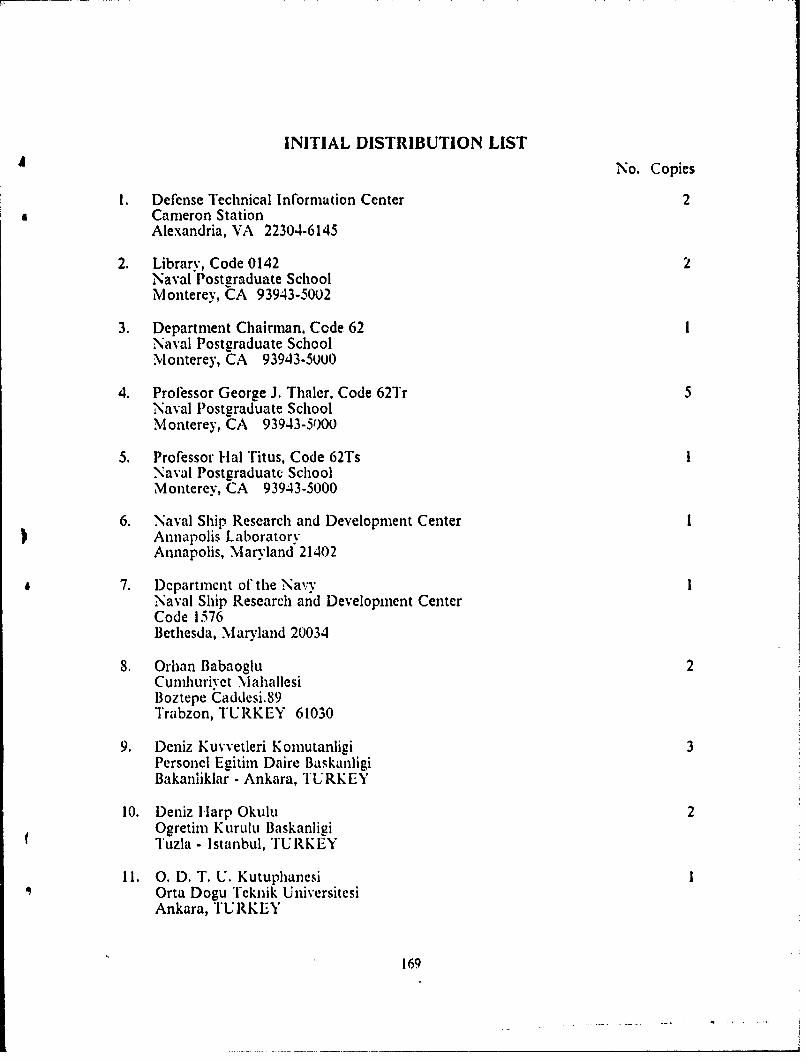
INITIAL DISTRIBUTION LIST

No. Copies

1. Defense Technical Information Center 2Cameron StationAlexandria, VA 22304-6145

2. Library, Code 0142 2Naval Postgraduate SchoolMonterey, CA 93943-5002

3. Department Chairman. Code 62 1Naval Postgraduate SchoolMonterey, CA 93943-5000

4. Professor George J. Thaler, Code 62Tr 5Naval Postgraduate SchoolMonterey, CA 93943-5000

5. Professor Hal Titus, Code 62Ts INaval Postgraduate SchoolMonterey, CA 93943-5000

6. Naval Ship Research and Development Center 1Annapolis LaboratoryAnnapolis, Maryland 21402

7. Dcpartment of the Navy 1Naval Ship Research and Development CenterCode 1.576Bethesda, Maryland 20034

8. Orhan Babaoglu 2Cumhurivet NiahallesiBoztepe Caddesi.89Trabzon, TURKEY 61030

9. Deniz Kuvvetleri Komutanligi 3Personel Egitim Daire BaskanligiBakanliklar - Ankara, TURKEY

10. Deniz Harp Okulu 2Ogretim Kurulu BaskanligiTuzla - Istanbul, TURKEY

11. 0. D. T. U. Kutuphanesi 1Orta Dogu Teknik UniversitesiAnkara, T'URKEY

169

12. 1-lacettepe Universitesi Kutuphanesi1-lacettepe Utiiv ersitesi, BeytepeAnkara, TURKEY

13. Denizalti Filosu KomutanligiGolcukKocachi, TURKEY

14. Denizalti Egitim Mcrkezi KoinutanligiGolcukKocaclIi, TURKEY

15. Gurkan TurkesSMC 21983 NI'SMonterey , CA 93943

170

Documents

NAVAL POSTGRADUATE SCHOOL · NAVAL POSTGRADUATE SCHOOL Monterey, California In 0 THESIS DESIGNING AN AUTOMATIC CONTROL SYSTEM ... Master's Thesis From To December 1988 183 16 Supplementary