Embed Size (px)
Citation preview

NAVAL POSTGRADUATE
SCHOOL
MONTEREY, CALIFORNIA
THESIS
Approved for public release; distribution is unlimited
AN IMPROVED THERMAL BLOOMING MODEL FOR THE LASER PERFORMANCE CODE ANCHOR
by
Joseph C. Collins
June 2016
Thesis Advisor: Keith R. Cohn Second Reader: Joseph Blau

THIS PAGE INTENTIONALLY LEFT BLANK
i
REPORT DOCUMENTATION PAGE Form Approved OMB No. 0704-0188
Public reporting burden for this collection of information is estimated to average 1 hour per response, including the time for reviewing instruction, searching existing data sources, gathering and maintaining the data needed, and completing and reviewing the collection of information. Send comments regarding this burden estimate or any other aspect of this collection of information, including suggestions for reducing this burden, to Washington headquarters Services, Directorate for Information Operations and Reports, 1215 Jefferson Davis Highway, Suite 1204, Arlington, VA 22202-4302, and to the Office of Management and Budget, Paperwork Reduction Project (0704-0188) Washington DC 20503. 1. AGENCY USE ONLY (Leave blank)
2. REPORT DATE June 2016
3. REPORT TYPE AND DATES COVERED Master’s thesis
4. TITLE AND SUBTITLE AN IMPROVED THERMAL BLOOMING MODEL FOR THE LASER PERFORMANCE CODE ANCHOR
5. FUNDING NUMBERS
6. AUTHOR(S) Joseph C. Collins
7. PERFORMING ORGANIZATION NAME(S) AND ADDRESS(ES) Naval Postgraduate School Monterey, CA 93943-5000
8. PERFORMING ORGANIZATION REPORT NUMBER
9. SPONSORING /MONITORING AGENCY NAME(S) AND ADDRESS(ES)
N/A
10. SPONSORING / MONITORING AGENCY REPORT NUMBER
11. SUPPLEMENTARY NOTES The views expressed in this thesis are those of the author and do not reflect the official policy or position of the Department of Defense or the U.S. Government. IRB Protocol number ____N/A____.
12a. DISTRIBUTION / AVAILABILITY STATEMENT Approved for public release; distribution is unlimited
12b. DISTRIBUTION CODE A
13. ABSTRACT (maximum 200 words)
Laser weapon systems, unlike conventional weapons, are heavily dependent upon the ever-changing atmospheric conditions in their employment theater. In order to understand the operational effectiveness of a laser weapon, the performance limits due to atmospheric conditions need to be understood. ANCHOR, a laser performance scaling code developed at the Naval Postgraduate School, is one such code used to model a laser’s effectiveness for a variety of atmospheric conditions.
This thesis focuses on the calibration of ANCHOR’s thermal blooming model. In the absence of turbulence, thermal blooming is generally well understood and the thermal blooming Strehl ratio is well defined. When turbulence is coupled with thermal blooming, however, the thermal blooming Strehl ratio is exceedingly difficult to quantify using scaling codes. This thesis calibrates ANCHOR’s thermal blooming model using the full wave propagation code TBWaveCalc by adjusting the coefficients of an analytical formula to “best fit” the TBWaveCalc results over a wide variety of initial conditions.
14. SUBJECT TERMS thermal blooming, atmospheric propagation, laser, scaling code, Strehl ratio, ANCHOR, COAMPS, NAVSLaM, LEEDR
15. NUMBER OF PAGES
77 16. PRICE CODE
17. SECURITY CLASSIFICATION OF REPORT
Unclassified
18. SECURITY CLASSIFICATION OF THIS PAGE
Unclassified
19. SECURITY CLASSIFICATION OF ABSTRACT
Unclassified
20. LIMITATION OF ABSTRACT
UU NSN 7540-01-280-5500 Standard Form 298 (Rev. 2-89)
Prescribed by ANSI Std. 239-18

ii
THIS PAGE INTENTIONALLY LEFT BLANK

iii
Approved for public release; distribution is unlimited
AN IMPROVED THERMAL BLOOMING MODEL FOR THE LASER PERFORMANCE CODE ANCHOR
Joseph C. Collins Lieutenant, United States Navy
B.S., The Citadel, 2010
Submitted in partial fulfillment of the requirements for the degree of
MASTER OF SCIENCE IN APPLIED PHYSICS
from the
NAVAL POSTGRADUATE SCHOOL
June 2016
Approved by: Keith R. Cohn Thesis Advisor
Joseph Blau Second Reader
Kevin B. Smith Chair, Department of Physics

iv
THIS PAGE INTENTIONALLY LEFT BLANK

v
ABSTRACT
Laser weapon systems, unlike conventional weapons, are heavily dependent upon
the ever-changing atmospheric conditions in their employment theater. In order to
understand the operational effectiveness of a laser weapon, the performance limits due to
atmospheric conditions need to be understood. ANCHOR, a laser performance scaling
code developed at the Naval Postgraduate School, is one such code used to model a
laser’s effectiveness for a variety of atmospheric conditions.
This thesis focuses on the calibration of ANCHOR’s thermal blooming model. In
the absence of turbulence, thermal blooming is generally well understood and the thermal
blooming Strehl ratio is well defined. When turbulence is coupled with thermal
blooming, however, the thermal blooming Strehl ratio is exceedingly difficult to quantify
using scaling codes. This thesis calibrates ANCHOR’s thermal blooming model using the
full wave propagation code TBWaveCalc by adjusting the coefficients of an analytical
formula to “best fit” the TBWaveCalc results over a wide variety of initial conditions.

vi
THIS PAGE INTENTIONALLY LEFT BLANK
vii
TABLE OF CONTENTS
I. INTRODUCTION .................................................................................................1
II. OVERVIEW OF DIRECTED ENERGY (DE) WEAPONS ..............................3A. HISTORY ...................................................................................................3B. ADVANTAGES .........................................................................................4C. TECHNOLOGIES .....................................................................................4D. LAWS AND PONCE .................................................................................6
III. OVERVIEW OF ATMOSPHERIC CODES ......................................................9A. ANCHOR ....................................................................................................9
1. ANCHOR Methodology ..............................................................11B. NAVY ATMOSPHERIC VERTICAL SURFACE LAYER
MODEL (NAVSLaM) .............................................................................15C. THE LASER ENVIRONMENTAL EFFECTS DEFINITION
AND REFERENCE (LEEDR) ................................................................17D. COUPLED OCEAN/ATMOSPHERE MESOSCALE
PREDICTION SYSTEM (COAMPS) ...................................................17E. LASER PROPAGATION EXAMPLE: LEEDR ..................................18F. LASER PROPAGATION EXAMPLE: COAMPS/NAVSLaM ..........23
IV. THERMAL BLOOMING ...................................................................................27A. THERMAL BLOOMING OVERVIEW ...............................................27B. THERMAL BLOOMING THEORY .....................................................28C. THERMAL BLOOMING CALIBRATION .........................................31
1. Results: Wind = 10 m/s, D = 30 cm, Range = 5 km ...................322. Results: Wind = 10 m/s, D = 30 cm, Slant Range = 5 km .........363. Results: Wind = 5 m/s, D = 30 cm, Range = 5 km .....................384. Results: Wind = 10 m/s, D = 10 cm, Range = 5 km ...................395. Results: Wind = 10 m/s, D = 50 cm, Range = 5 km ...................426. Results: Wind = 10 m/s, D = 30 cm, Range = 8 km ...................447. Results: Wind = 5 m/s, D = 30 cm, Range = 8 km .....................458. Results: Wind = 5 m/s, D = 30 cm, Range = 1 km .....................469. Results: Wind = 20 m/s, D = 30 cm, Range = 5 km ...................48

viii
V. CONCLUSION ....................................................................................................53
LIST OF REFERENCES ................................................................................................55
INITIAL DISTRIBUTION LIST ...................................................................................57

ix
LIST OF FIGURES
Figure 1. Example of solid state laser components .....................................................5
Figure 2. ANCHOR 3D engagement volume ...........................................................10
Figure 3. Laser diffraction simulation for strong and weak turbulence ....................14
Figure 4. NAVSLaM output of Cn2 vs. height for different air/sea temperature
differences in the marine base layer ...........................................................16
Figure 5. ANCHOR: Time-averaged irradiance vs. target range and altitude, for a 100 kW laser. .....................................................................................18
Figure 6. ANCHOR: Time-averaged irradiance vs. longitudinal range and latitudinal range, for a 100 kW laser. .........................................................19
Figure 7. ANCHOR: Power-in-the-bucket vs. target range and altitude for a 100 kW laser. .............................................................................................20
Figure 8. ANCHOR: Power-in-the-bucket vs. longitudinal range and latitudinal range, for a 100 kW laser ..........................................................21
Figure 9. ANCHOR: Required dwell time vs. target range and altitude, for a 100 kW laser ..............................................................................................22
Figure 10. ANCHOR: Required dwell time vs. longitudinal range and latitudinal range, for a 100 kW laser. .........................................................23
Figure 11. ANCHOR: Time-averaged irradiance vs. target range and altitude, for a 100 kW laser using COAMPS, NAVSLaM, and LEEDR. ...............24
Figure 12. ANCHOR: Power-in-the-bucket vs. target range and altitude for a 100 kW laser, using COAMPS, NAVSLaM, and LEEDR. .......................25
Figure 13. ANCHOR: Required dwell time vs. target range and altitude for a 100 kW laser, using COAMPS, NAVSLaM, and LEEDR. .......................25
Figure 14. Laser diffraction simulation highlighting thermal blooming effects in the atmosphere ...........................................................................................27
Figure 15. Inverse Strehl ratio plotted against laser output power for Cn2 = 0 ............32
Figure 16. Inverse Strehl ratio plotted against laser output power for Cn2 = 4x10-
16 m-2/3 ........................................................................................................33
x
Figure 17. Inverse Strehl ratio plotted against laser output power for Cn2 = 8x10-
16 m-2/3 ........................................................................................................34
Figure 18. Inverse Strehl ratio plotted against laser output power for Cn2 = 4x10-
15 m-2/3 ........................................................................................................34
Figure 19. Inverse Strehl ratio plotted against laser output power for Cn2 = 1x10-
14 m-2/3 ........................................................................................................35
Figure 20. Inverse Strehl ratio plotted against laser output power for Cn2 =
1.22x10⁻¹⁴ m-2/3 ...........................................................................................35
Figure 21. Inverse Strehl ratio plotted against laser output power for Cn2 = 2x10-
14 m-2/3 ........................................................................................................36
Figure 22. Inverse Strehl ratio plotted against laser output power for Cn2 =
1.7x10⁻¹⁵ m-2/3 at the surface and a target altitude of 100 m ......................37
Figure 23. Inverse Strehl ratio plotted against laser output power for Cn2 = 9x10-
15 m-2/3 at the surface and a target altitude of 1000 m ................................37
Figure 24. Inverse Strehl ratio plotted against laser output power for Cn2 = 4x10-
16 m-2/3 ........................................................................................................38
Figure 25. Inverse Strehl ratio plotted against laser output power for Cn2 = 8x10-
16 m-2/3 ........................................................................................................39
Figure 26. Inverse Strehl ratio plotted against laser output power for Cn2 = 4x10-
16 m-2/3 ........................................................................................................40
Figure 27. Inverse Strehl ratio plotted against laser output power for Cn2 = 8x10-
16 m-2/3 ........................................................................................................40
Figure 28. Inverse Strehl ratio plotted against laser output power for Cn2 = 4x10-
15 m-2/3 ........................................................................................................41
Figure 29. Inverse Strehl ratio plotted against laser output power for Cn2 = 1x10-
14 m-2/3 ........................................................................................................41
Figure 30. Inverse Strehl ratio plotted against laser output power for Cn2 = 4x10-
16 m-2/3 ........................................................................................................42
xi
Figure 31. Inverse Strehl ratio plotted against laser output power for Cn2 = 8x10-
16 m-2/3 ........................................................................................................43
Figure 32. Inverse Strehl ratio plotted against laser output power for Cn2 = 1x10-
14 m-2/3 ........................................................................................................43
Figure 33. Inverse Strehl ratio plotted against laser output power for Cn2 = 8x10-
16 m-2/3 ........................................................................................................44
Figure 34. Inverse Strehl ratio plotted against laser output power for Cn2 = 4x10-
15 m-2/3 ........................................................................................................45
Figure 35. Inverse Strehl ratio plotted against laser output power for Cn2 = 8x10-
16 m-2/3 ........................................................................................................46
Figure 36. Inverse Strehl ratio plotted against laser output power for Cn2 = 8x10-
16 m-2/3 ........................................................................................................47
Figure 37. Inverse Strehl ratio plotted against laser output power for Cn2 = 4x10-
15 m-2/3 ........................................................................................................47
Figure 38. Inverse Strehl ratio plotted against laser output power for Cn2 = 1x10-
14 m-2/3 ........................................................................................................48
Figure 39. Inverse Strehl ratio plotted against laser output power for Cn2 = 0 ............49
Figure 40. Inverse Strehl ratio plotted against laser output power for Cn2 = 4x10-
16 m-2/3 ........................................................................................................49
Figure 41. Inverse Strehl ratio plotted against laser output power for Cn2 = 8x10-
16 m-2/3 ........................................................................................................50
Figure 42. Inverse Strehl ratio plotted against laser output power for Cn2 = 4x10-
15 m-2/3 ........................................................................................................50
Figure 43. Inverse Strehl ratio plotted against laser output power for Cn2 = 1x10-
14 m-2/3 ........................................................................................................51

xii
THIS PAGE INTENTIONALLY LEFT BLANK

xiii
LIST OF TABLES
Table 1. ANCHOR example, laser parameters ........................................................18

xiv
THIS PAGE INTENTIONALLY LEFT BLANK

xv
LIST OF ACRONYMS AND ABBREVIATIONS
COAMPS Coupled Ocean/Atmosphere Mesoscale Prediction System
DE Directed Energy DOD Department of Defense
FEL Free-electron Laser HEL High Energy Laser
LaWS Laser Weapons System LEEDR Laser Environment Effects Definition and Reference
MIRACL Mid-Infrared Advanced Chemical Laser NACL Navy-ARPA Chemical Laser
NAVSLaM Navy Atmospheric Vertical Surface Layer Model NPS Naval Postgraduate School
SSL Solid-State Laser

xvi
THIS PAGE INTENTIONALLY LEFT BLANK

xvii
ACKNOWLEDGMENTS
I would like to thank my thesis advisor, Professor Keith Cohn, and my second
reader, Professor Joseph Blau, for their insight and assistance in completing this thesis. I
would also like to thank Dr. Conor Pogue for his help and guidance in completing the
research for this thesis.

xviii
THIS PAGE INTENTIONALLY LEFT BLANK
1
I. INTRODUCTION
The feasibility of using directed energy (DE) weapons in a combat environment
has been studied extensively by the Department of Defense (DOD) for decades. In recent
years the Navy has developed a shipboard laser weapons system (LaWS) and deployed it
onboard the USS Ponce in the Persian Gulf for testing and evaluation. While this can be
seen as a step toward fielding lasers and other DE weapons aboard Naval platforms, there
are still several hurdles that must be overcome. One such issue is the ability to accurately
predict an effective engagement range. Laser weapons are acutely sensitive to
atmospheric changes in their employment area, especially in the maritime environment.
In order for a laser to be effective as a defensive weapon, the operator needs to
understand the potential limitations of the laser in any environment before employment.
The ANCHOR laser performance code was developed by the Naval Postgraduate School
(NPS) Physics DE Group to meet this need while being extremely fast and adaptable.
Given initial laser parameters and atmospheric inputs from atmospheric modeling codes,
ANCHOR can compute laser effectiveness in a matter of seconds. The scope of this
thesis focuses on the ANCHOR code, particularly in how it models the effects of thermal
blooming. Specifically, ANCHOR’s thermal blooming model was calibrated against
TBWaveCalc, a full diffraction code published by MZA, over a wide variety of initial
conditions.
An outline of this thesis includes a brief discussion of directed energy weapons,
an overview of laser codes including ANCHOR, and the thermal blooming calibration
method and results.

2
THIS PAGE INTENTIONALLY LEFT BLANK

3
II. OVERVIEW OF DIRECTED ENERGY (DE) WEAPONS
A. HISTORY
Since the invention of the laser in the early 1960s, the military has been heavily
invested in its maturation and potential for battlefield application. In 1971, the U.S Navy
established a dedicated High Energy Laser (HEL) program office in order to study and
develop HEL technology capable of defending naval vessels at sea from aerial threats
like anti-ship cruise missiles. Early testing was centered on CO2 gas dynamic laser
technology, with a wavelength of approximately 10.6 µm, the highest power laser at the
time [1]. In 1973, it was demonstrated for the first time, using a continuous wave
deuterium fluoride (DF) laser, that chemical laser technology could be scaled to high
powers. With an output wavelength of around 3.8 µm, chemical lasers immediately
became a better option than CO2 lasers for naval applications due to superior atmospheric
propagation in the maritime environment [1].
The Navy-ARPA Chemical Laser (NACL) was the Navy’s first attempt to assess
the plausibility of using a chemical HEL for fleet defense using a scaled-up DF laser. In
1978, using the NACL, the Navy successfully demonstrated the ability to engage and
destroy missiles in flight – specifically TOW anti-tank missiles flying at low altitude with
crossing trajectories at high subsonic speeds [1]. Leveraging the knowledge gained from
the NACL, the Navy set it sights on developing a laser capable of reaching much higher
power levels, developing the megawatt class Mid-InfraRed Advanced Chemical Laser
(MIRACL) in the early 1980s. Throughout the 1980s, MIRACL was used by the DOD
for a variety of damage and vulnerability tests at the High Energy Laser System Test
Facility at White Sands, New Mexico, ultimately, in 1989 demonstrating the capability of
engaging a supersonic threat [1]. Despite the promising performance of chemical lasers,
the Navy ultimately ceased its research citing logistical and safety issues associated with
the hazardous chemicals in a shipboard environment.

4
As technology matured, the Navy began to focus on using Solid-State Lasers
(SSLs) for shipboard applications, due to their increased propagation at shorter
wavelengths, culminating in the deployment of the LaWS on the USS Ponce in 2014.
B. ADVANTAGES
A major drive toward the use of HEL weapons has been their perceived advantage
in combat, specifically when battling an asymmetric threat. One advantage is the ability
to place a focused spot of light on a target instead of firing a projectile. The HEL beam
can inflict a varying amount of thermal damage on target, delivering a high amount of
energy to a localized target, thus minimizing collateral damage and increasing mission
kill effectiveness. The HEL weapon can begin delivering energy to the target almost
instantly—at the speed of light—ideal for long-range targets and when a quick reaction is
necessary to combat the threat. As an electric weapon, the magazine is only limited by
the available power onboard, so the weapon can conduct multiple shots without the need
to reload, and the cost per shot is equivalent to the cost of the fuel required to produce the
power. Along with these advantages, there are currently several issues that could limit
their effectiveness. The weapon requires the target to be in line of sight; it cannot engage
targets over the horizon or low-flying threats obscured by waves. A finite dwell time is
required to accrue damage (a typical engagement could last several seconds) limiting its
ability to be used against simultaneous threats. An HEL weapon is also susceptible to
atmospheric conditions and can be limited due to rain, haze, fog, or similar weather
phenomena. As the technology matures, many of these disadvantages can be mitigated,
making their advantages much more enticing.
C. TECHNOLOGIES
The term laser stands for Light Amplification by Stimulated Emission of
Radiation. By its nature, a laser increases or amplifies light waves after they have been
generated by spontaneous emission. A laser generally consists of four components: laser
pumping source, a gain or amplifying medium, total reflecting mirror, and partial
reflecting mirror illustrated in Figure 1 [2].

5
Figure 1. Example of solid state laser components
In recent years, naval research into HELs has centered on SSLs and Free-Electron Lasers
(FELs). Vastly different systems, SSLs represent the best hope for attaining high powers
today, while FELs represent the potential for high power, efficient lasers with a variety of
military relevant applications for the future.
SSLs, which utilize solid-state materials as their gain medium, represent a large
percentage of current HEL research. SSLs generally consist of crystalline or glass host
materials with specific atomic ions—rare earth or transition-metal elements—grown into
the host material to act as the lasing species (dopant ions). SSLs use optical pumping,
either through diode-pumping or flashlamp-pumping, to create the population inversion
necessary for the lasing process. Advantages of SSLs are their relative maturity, compact
and lightweight design, and efficiency. For naval applications, SSLs are particularly
enticing due to their lack of harmful bi-products such as hazardous chemicals or ionizing
radiation, and due to the fact that they output wavelengths that propagate extremely well
in clear weather, particularly Ytterbium lasers with wavelengths of approximately 1 µm.
Unfortunately, there are several potential barriers to their full-scale use in military
applications. Of particular note is the fact that the glass/crystalline host materials
generally have a low thermal conductivity, which would limit their average power output
due to an inability to eliminate waste heat. A related issue is that in order to be effective
as an HEL weapon, many SSLs must be combined, which can limit beam quality or
increase the complexity of the laser system.

6
Free Electron Lasers generate light by sending a relativistic beam of electrons
through a periodic magnetic field. As these free electrons move through vacuum, the
magnetic field causes them to undulate and therefore produce light. There are two types
of FELs, oscillator FELs and amplifier FELs. An oscillator FEL is made up of three core
elements: an electron beam and the accelerator to produce it, the undulator magnet, and
an optical resonator. Amplifier FELs utilize a seed laser source in place of an optical
resonator [3]. As the technology matures, the use of FELs as a HEL weapon becomes
increasingly advantageous. Unlike other types of lasers, FELs are tunable and can vary
the output wavelength for best atmospheric transparency. FELs are also naturally scalable
and can potentially vary output power from the kW to MW levels depending on the
target. Unlike the current configurations for SSLs, FELs can have excellent beam quality
even at high power. Unfortunately for FELs, there are currently several roadblocks to
their implementation onboard naval platforms: FELs are generally large (on the order of
20 m in length), heavy, and expensive, requiring large research teams to operate and
maintain [3]. The technology is not yet mature enough for military applications.
D. LAWS AND PONCE
The Laser Weapons System was developed to test the capabilities and feasibility
of solid-state lasers onboard naval platforms. LaWS was designed primarily as a cost
effective defense against a swarm threat, small drones, or fast-attack craft in the water.
The LaWS demonstrator incoherently combines several commercial off-the-shelf fiber
SSLs, each with a power of abut 5 kW and a total power of approximately 30 kW, a beam
quality factor, M2, of 17, and a wavelength of 1.064 µm [4]. In the summer of 2014
LaWS was installed on the Afloat Forward Staging Base, USS Ponce, for a 12-month
demonstration in a combat relevant, maritime environment. Prior to its deployment on the
Ponce, LaWS had multiple successful tests, including successful engagements at
NAWCWD China Lake, and maritime engagements off the coast of Southern California
onboard the USS Dewey [4]. Following the demonstration period onboard Ponce, the
LaWS system was cleared to remain in place for the foreseeable future as an operational
asset, and is currently being used for daily target identification and watch stander
training. The success of the LaWS systems has paved the wave for the Solid-State Laser

7
– Technical Maturation program, which has the goal of operationally fielding a 100 kW
laser on surface combatants within the next five years.

8
THIS PAGE INTENTIONALLY LEFT BLANK

9
III. OVERVIEW OF ATMOSPHERIC CODES
A. ANCHOR
The NPS laser performance code, ANCHOR, is a MATLAB script that rapidly
can explore millions of different initial condition combinations. ANCHOR has been
calibrated against WaveTrain, an industry-developed full diffraction code that has been
validated against existing codes that have been found to be in agreement with theory and
experimentation [5]. ANCHOR produces results that are in approximate agreement with
WaveTrain, but ANCHOR runs many orders of magnitude faster than WaveTrain. Unlike
full diffraction codes like WaveTrain, which solve the paraxial wave equation
numerically and provide irradiance profile information for each time step, ANCHOR uses
well-known, experimentally validated analytical scaling laws to provide time-averaged
values of irradiance, power-in-the-bucket, and other figures of merit.
Currently, there exist several variations of the ANCHOR code—S, L, and P—
depending upon the desired results. ANCHOR S, the simplest version, assumes the
atmospheric conditions, including the effects of turbulence, the total extinction, and the
wind speed and direction remain constant along the beam path of the laser. Since the
atmospheric conditions remain constant, ANCHOR S does not need output from
atmospheric modeling codes; instead, the user specifies the atmospheric conditions for
each study directly in the script. Based on the user defined input values, ANCHOR S
outputs the time-averaged irradiance, time-averaged power-in-the-bucket, and dwell time.
The L and P versions allow the atmospheric parameters to vary along the beam
path and therefore require output from atmospheric modeling codes in order to obtain this
information. ANCHOR L and P both output 2D slices through the 3D engagement
volume of the time-averaged irradiances, time-averaged powers-in-the-bucket, and dwell
times.
ANCHOR L provides a horizontal slice for each figure of merit, showing changes
in laser performance with varying altitude and range along a constant bearing from the
laser platform. Instead of horizontal slices, ANCHOR P provides vertical slices from a
10
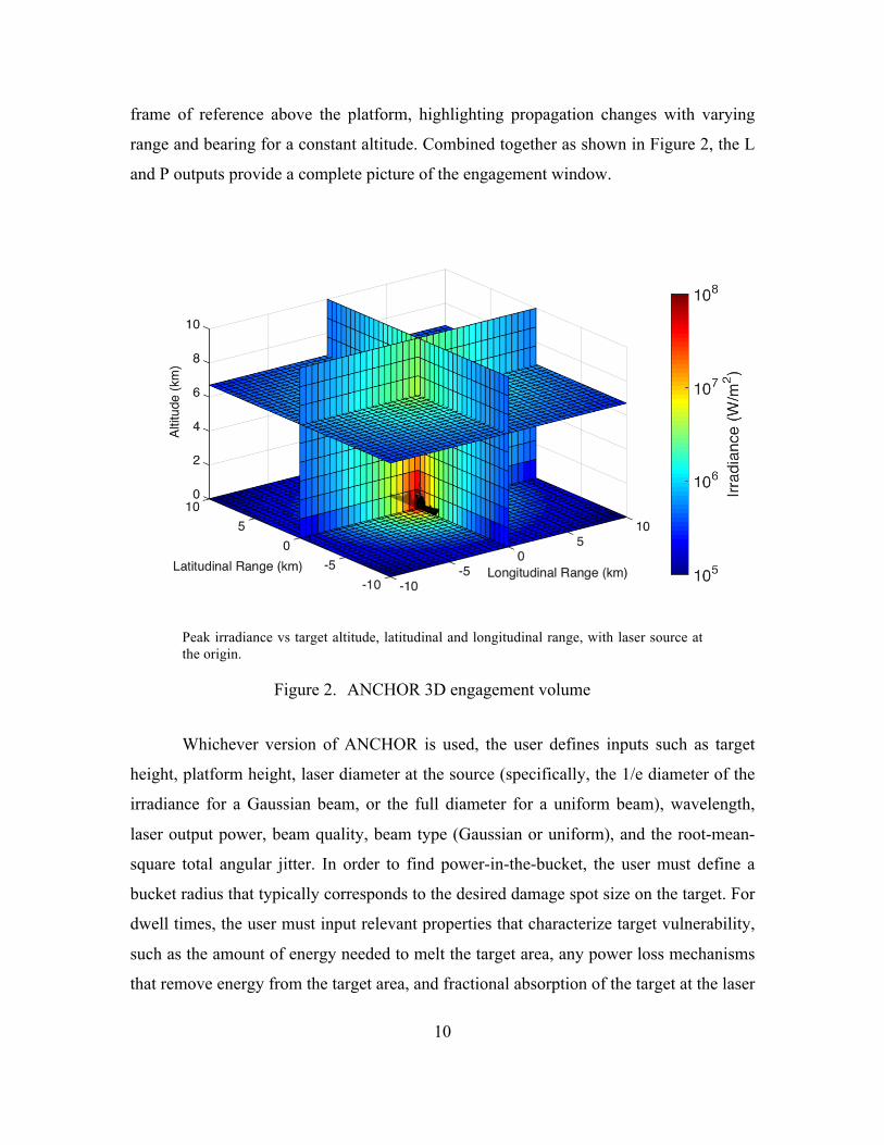
frame of reference above the platform, highlighting propagation changes with varying
range and bearing for a constant altitude. Combined together as shown in Figure 2, the L
and P outputs provide a complete picture of the engagement window.
Peak irradiance vs target altitude, latitudinal and longitudinal range, with laser source at the origin.
Figure 2. ANCHOR 3D engagement volume
Whichever version of ANCHOR is used, the user defines inputs such as target
height, platform height, laser diameter at the source (specifically, the 1/e diameter of the
irradiance for a Gaussian beam, or the full diameter for a uniform beam), wavelength,
laser output power, beam quality, beam type (Gaussian or uniform), and the root-mean-
square total angular jitter. In order to find power-in-the-bucket, the user must define a
bucket radius that typically corresponds to the desired damage spot size on the target. For
dwell times, the user must input relevant properties that characterize target vulnerability,
such as the amount of energy needed to melt the target area, any power loss mechanisms
that remove energy from the target area, and fractional absorption of the target at the laser
11
wavelength. In addition to the user defined properties, atmospheric data for ANCHOR
versions L and P must be loaded into the MATLAB environment from a code such as
LEEDR (the Laser Environmental Effects Definition and Reference, developed by the
Air Force Institute of Technology Center for Directed Energy), NAVSLaM (the Navy
Atmospheric Vertical Surface Layer Model, developed by the Meteorology department of
the Naval Postgraduate School), or COAMPS (the Coupled Ocean/Atmosphere
Mesoscale Prediction System, developed by the Marine Meteorology Division of the
Naval Research Lab). This study utilizes all three atmospheric codes.
1. ANCHOR Methodology
ANCHOR utilizes the following equation to calculate time-averaged irradiance
at the target:
I =Po exp − ε z( )dz∫( )
π wtot2 ⋅STB , (1)
where is the output power of the laser at the beam director, z is the distance coordinate
along the path from the beam director to the target, is the total extinction coefficient
(i.e., the combination of the effects of absorption and scattering) provided by the
atmospheric modeling code, is the time-averaged spot radius (1/e in irradiance) on
target, and is the thermal blooming Strehl ratio.
In order to estimate power-in-the-bucket for a given bucket radius rBKT , the
following equations are used:
PBKT =π ⋅ I ⋅rBKT
2
π ⋅ I ⋅weff2
⎧⎨⎪
⎩⎪
ifif
rBKT < weff
rBKT > weff
. (2)
Here, weff is the effective spot radius on target and is the result of the increase in spot size
due to thermal blooming. It is calculated by dividing the time-averaged spot radius on
target due to linear effects only, , by the square root of the thermal blooming Strehl
ratio,
I
Po
ε
wtot
STB
wtot

12
weff ≡wtot
STB . (3)
In order to calculate dwell time to melt a certain volume of the target, ANCHOR
uses the following equations:
Pmelt = FABS ⋅PBKT − Ploss (4)
. (5)
In this case, FABS is the fractional target absorption; is the power available after
subtracting parasitic losses due to conduction and radiation, which depends on the
emissivity and thermal conductivity of the target material; and is the amount of
energy to melt a certain volume of the target and depends upon the target’s material
properties, specifically, the melting temperature, heat capacity, and heat of fusion.
a. Time-averaged spot radius on target
There are several contributions to the spot size of a laser beam on a target,
including diffraction, turbulence, jitter, and thermal blooming. Thermal blooming is a
non-linear effect that is accounted for by the 𝑆!" factor in equation 1 and will be
discussed in greater detail in another chapter. The other three effects contribute to the
overall time-averaged spot size by (approximate) addition in quadrature [6]:
wtot2 = wd
2 +wt2 +wj
2 , (6)
where is the radius of the laser beam at the target solely due to diffraction in a
vacuum, is the radius solely due to turbulence-induced beam spreading, and is the
root-mean-square radius due to the angular jitter.
For a laser beam in a vacuum, the time-averaged spot radius is only a function of
diffraction and represents the ideal spot radius for a given range and known beam
quality. The focus spot of a laser beam in a vacuum can be calculated by the following
equation [6]:
wd = M2 2lkD
(Gaussian). (7)
tdwell =Qmelt
Pmelt
Pmelt
Qmelt
wd
wt wj
wd
13
Here, is a measure of the beam quality of a laser, is the range from the laser
source to the target, and k = 2π λ is the wavenumber. For a Gaussian beam, D is equal to
the 1/e diameter of the irradiance at the source. In the case of a uniform beam, where D is
equal to the full diameter of the irradiance at the source, equation 7 becomes:
wd = M2 4lkD
(Uniform). (8)
ANCHOR utilizes the simplified equations to determine the diffraction-limited
spot radius when calculating the time-averaged spot radius on target.
Outside a vacuum, the presence of atmospheric turbulence plays a role in the
overall time-averaged spot radius as shown in equation 6. Turbulence-induced spreading
of laser beams is generally caused by small-scale turbulent horizontal motion in the
atmosphere that results from vertical temperature and density differences, wind shear,
and convective air flow [3]. These atmospheric effects cause changes in the refractive
index of the air along the path and in turn cause the beam to spread and the time-averaged
irradiance to decrease. Many studies have been conducted in order to quantify
electromagnetic wave propagation through turbulent media; of particular note is the work
done by Fried that led to the development of the Fried parameter ro , which can be used to
describe the effects of turbulence on laser propagation [7]. The Fried parameter defines
the diameter over which a laser beam can maintain transverse coherence throughout its
propagation distance. Typical values of ro are on the order of a few centimeters where
smaller values correspond to stronger turbulence. To calculate ro , the following equation
is commonly used [8]:
ro = 2.10[1.45k2 Cn
2
0
l
∫ (z)(1− zl)53dz]
− 35 (Spherical Wave). (9)
Here, k is the wavenumber, l is the distance from laser source to target, and Cn2 is the
refractive structure constant. The Cn2 value was first theoretically parameterized by
Kolmogorov and is experimentally measured; higher Cn2 values are associated with
stronger turbulence, and it is generally a function of altitude with larger Cn2 occurring
near the surface [3].
M 2 l

14
Plot A in Figure 3 shows a full diffraction simulation of a laser propagating over a
range of 5 km in weak turbulence, Cn2 ≈10−18m−2 3 ; here, the beam maintains transverse
coherence throughout the propagation path so the result is a circular spot at the focus.
Plot b in Figure 3, shows the beam propagation over a range of 5 km in stronger
turbulence, Cn2 ≈10−14m−2 3 , and the resulting spot begins to break up into beamlets and
spread out. The intensity at the focus is denoted by a color scale, with red indicating the
highest peak irradiance and blue indicating the lowest.
a.) Weak turbulence, b.) Strong turbulence,
Figure 3. Laser diffraction simulation for strong and weak turbulence
Once the Fried parameter has been calculated by ANCHOR using the Cn2 profile
from the atmospheric modeling code, the turbulence-induced beam spreading can be
calculated using the following equation [8]:
wt =wd
M 2Dro
. (10)
Here, wt represents the contribution to the spot size from the total turbulence, including
the effects of both long and short-term turbulence. The total turbulence term is used in the
calculation of the time-averaged spot radius on target.
Cn2 ≈10−18m−2/3 Cn
2 ≈10−14m−2/3

15
The spatial width due to jitter, wj, has a varying effect on the time-averaged spot
radius. The factors that contribute to the overall jitter are platform motion, and tracking
error [8]. The beam jitter can be calculated with the following equation [6]:
wj = θrmsl . (11)
where θrms is defined as the effective angular jitter from all sources.
b. Thermal Blooming Strehl Ratio
Thermal blooming is a nonlinear propagation effect resulting from the absorption
of laser radiation by molecules and aerosols in the atmosphere that alters the air density
along the propagation path. The thermal blooming Strehl ratio, , is the ratio of the
laser’s irradiance with thermal blooming to the laser’s irradiance without thermal
blooming; therefore, 𝑆!" ranges from ~0 (for strong thermal blooming) to ~1 (for weak
thermal blooming). Depending on the laser output power and the propagation range,
thermal blooming can become the dominant factor in determining laser effectiveness.
How ANCHOR calculates 𝑆!" will be discussed in the following chapter.
B. NAVY ATMOSPHERIC VERTICAL SURFACE LAYER MODEL (NAVSLaM)
NAVSLaM is a model developed by the Meteorology Department at NPS and is
used by the Navy to calculate turbulence Cn2( ) profiles over the ocean up to
approximately 100 meters above sea level. NAVSLaM takes numerical weather
prediction model forecasts i.e. from COAMPS; weather data sets from sources like
NOAA and NAVMETOCCOM; or real-world observations of the wind speed, air and sea
temperatures, relative humidity, and pressure data; and outputs near-surface vertical
modified Cn2 profiles [9]. In order to calculate these profiles, NAVSLaM utilizes the
Monin-Obukhov similarity theory, which assumes that within the surface layer conditions
are horizontally homogenous and stationary, and that sensible heat, latent heat, and
turbulent fluxes of momentum do not vary with height [10]. When blended with models
such as COAMPS and LEEDR that calculate the upper-air refractivity profiles, a profile
STB

16
of the turbulence in the entirety of the engagement window can be obtained and imported
into ANCHOR to determine laser effectiveness.
In the maritime environment, the main source of turbulence in the surface
boundary layer is the air/sea temperature difference. When the temperature of the air is
less than the temperature of the sea, Tair<Tsea, the conditions are unstable, and there tends
to be higher turbulence at the surface, which then rapidly decreases with altitude. When
the temperature of the air is greater than the temperature of the sea, Tair>Tsea, the
conditions are stable, there tends to be less turbulence at the surface, and it tends to
remain relatively constant up to a few tens of meters above the surface.
In Figure 4, the wind speed is 1.9 m/s, the sea temperature is 90°F, the relative
humidity is 80%, and the pressure is 105 Pa at 1 m. The figure shows profiles, up to
20 m, highlighting the difference between stable conditions, when (red lines),
unstable conditions, when (green lines), and a neutral case, when (black
line). Where . This plot was generated using NAVSLaM.
Figure 4. NAVSLaM output of Cn2 vs. height for different air/sea temperature
differences in the marine base layer
Cn2
ΔT > 0ΔT < 0 ΔT = 0
ΔT = Tair −Tsea
17
C. THE LASER ENVIRONMENTAL EFFECTS DEFINITION AND REFERENCE (LEEDR)
LEEDR, developed by the Air Force Institute of Technology Center for Directed
Energy, is used to develop an atmospheric profile for a defined location. LEEDR utilizes
input parameters like the season, time of day, and relative humidity to calculate profiles
of “temperature, pressure, water vapor content, optical turbulence, atmospheric
particulates, and hydrometeors as they relate to layer transmission and path/background
radiance at any wavelength” for the defined location from the surface to an altitude of
100 km [11]. In order to calculate atmospheric profiles, LEEDR uses surface weather
models based on the season and time of the day in order to define the atmospheric
boundary layer. From this, LEEDR “computes the radiative transfer and propagation
effects from the vertical profile of meteorological variables,” providing the capability to
create realistic atmospheric profiles for a specified location [11]. The LEEDR
atmospheric profiles can then be exported to ANCHOR and used to model the laser’s
propagation in the maritime environment.
D. COUPLED OCEAN/ATMOSPHERE MESOSCALE PREDICTION SYSTEM (COAMPS)
COAMPS, developed by the Naval Research Lab Marine Meteorology Division,
is used to predict atmospheric conditions. COAMPS predicts wind, temperature, pressure,
clouds, and aerosols based on inputs from meteorological observations, satellite data, ship
reports, ocean observations, and bathymetry [12]. Because COAMPS calculates its initial
state based on observations, it is re-locatable and can be used worldwide. The COAMPS
forecast data can also be input into NAVSLaM to calculate the refractivity profile near
the surface. When the two models are blended together, an accurate model for the
engagement window can be imported into ANCHOR to determine laser effectiveness in a
quasi-real-world environment.
18
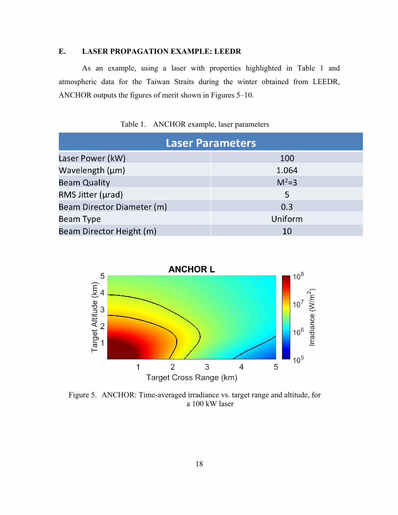
E. LASER PROPAGATION EXAMPLE: LEEDR
As an example, using a laser with properties highlighted in Table 1 and
atmospheric data for the Taiwan Straits during the winter obtained from LEEDR,
ANCHOR outputs the figures of merit shown in Figures 5–10.
Table 1. ANCHOR example, laser parameters
Figure 5. ANCHOR: Time-averaged irradiance vs. target range and altitude, for a 100 kW laser

19
The L variation of ANCHOR outputs an irradiance curve for the propagation path
along a constant bearing from platform to target (in this example 90°), with varying range
and altitude. The color scale on the right of the figure highlights the irradiance on target.
In Figure 5, the platform is located at the origin, which is also the region with highest
irradiance on target. The black contour lines correspond to irradiance thresholds, and
represent the relative hardness of a target. The contour line closest to the platform
corresponds to an irradiance of 10 MW/m2, and would be associated with a harder target.
The contour line farthest to the right of the platform corresponds to an irradiance of 1
MW/m2 and would be associated with a softer target. The contour line in the center
corresponds to an irradiance of 5 MW/m2.
Like the L variation, the P variation of ANCHOR outputs an irradiance curve
shown in Figure 6, however, the P variation outputs a curve of the propagation path for a
constant altitude—for this example 10 m, with varying bearing and range.
Figure 6. ANCHOR: Time-averaged irradiance vs. longitudinal range and latitudinal range, for a 100 kW laser
In Figure 6, the platform is at the center of the plot, the black contour lines represent the
same irradiance thresholds as Figure 5.

20
In order to calculate power-in-the-bucket, a bucket size must be identified.
Figures 7 and 8 are for a bucket radius of 5 cm.
Figure 7. ANCHOR: Power-in-the-bucket vs. target range and altitude for a 100 kW laser
Figure 7 is the ANCHOR L output for power-in-the-bucket. The curve shows that close
to the platform—at the origin—most of the laser power falls in the bucket. As range and
altitude increase, less power falls in the bucket. The contour line represents a threshold of
50 kW.
Similarly, Figure 8 shows the ANCHOR P output of power-in-the-bucket for the
same criteria.

21
Figure 8. ANCHOR: Power-in-the-bucket vs. longitudinal range and latitudinal range, for a 100 kW laser
Figure 8 shows that at the platform, near the center of the plot, the power-in-the-bucket
exceeds the threshold value and as the radius around the platform increases less power
falls in the bucket.
In order to calculate required dwell time for hard kill of a given target, several
material properties for the target are used to calculate Qmelt, FABS, and Ploss, discussed
previously in the ANCHOR methodology section. For this example a hard kill is defined
as melting a 5 cm radius, 3 mm thick piece of aluminum, Qmelt for the aluminum is
approximately 50 kJ, Ploss is approximately 2.5 kJ, and FABS is 15%. Using these values
ANCHOR produces the dwell time plots shown in Figures 9 and 10:
Latit
udin
al R
ange
(km
)
Longitudinal Range (km)

22
Plot of required dwell time for hard kill of a 100 cm2, 3 mm thick piece of aluminum
Figure 9. ANCHOR: Required dwell time vs. target range and altitude, for a 100 kW laser
For the L variation of ANCHOR shown in Figure 9, the color scale represents
required dwell times. The dark red is predominate after about 3 km on the horizontal axis
and shows that for this distance the dwell time diverges because Pmelt, the power available
to melt the target, is much less than the Ploss, the power lost to conduction and radiative
processes; the laser is ineffective at this range, at least for hard kills of this particular
target. The black contour line in this case represents the dwell time threshold of 5 s and
represents the maximum range for which a target with the parameters defined in this
section can be destroyed in 5 s.
23
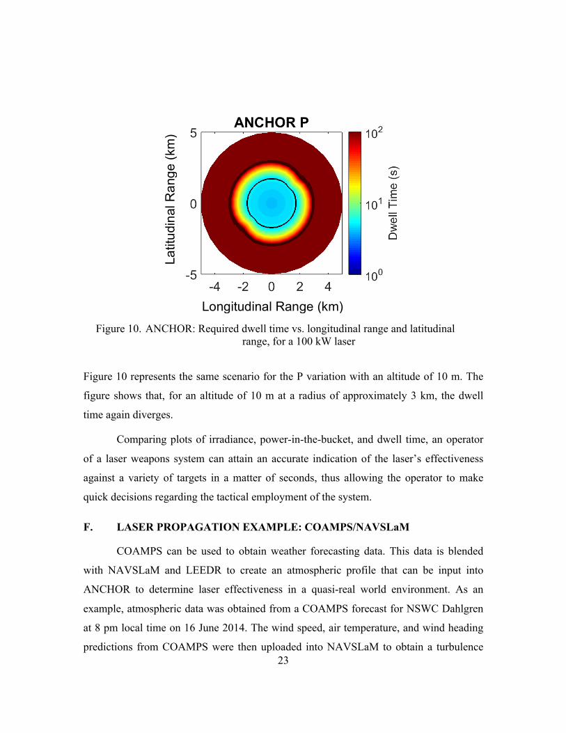
Figure 10. ANCHOR: Required dwell time vs. longitudinal range and latitudinal range, for a 100 kW laser
Figure 10 represents the same scenario for the P variation with an altitude of 10 m. The
figure shows that, for an altitude of 10 m at a radius of approximately 3 km, the dwell
time again diverges.
Comparing plots of irradiance, power-in-the-bucket, and dwell time, an operator
of a laser weapons system can attain an accurate indication of the laser’s effectiveness
against a variety of targets in a matter of seconds, thus allowing the operator to make
quick decisions regarding the tactical employment of the system.
F. LASER PROPAGATION EXAMPLE: COAMPS/NAVSLaM
COAMPS can be used to obtain weather forecasting data. This data is blended
with NAVSLaM and LEEDR to create an atmospheric profile that can be input into
ANCHOR to determine laser effectiveness in a quasi-real world environment. As an
example, atmospheric data was obtained from a COAMPS forecast for NSWC Dahlgren
at 8 pm local time on 16 June 2014. The wind speed, air temperature, and wind heading
predictions from COAMPS were then uploaded into NAVSLaM to obtain a turbulence
Longitudinal Range (km)
Latit
udin
al R
ange
(km
)
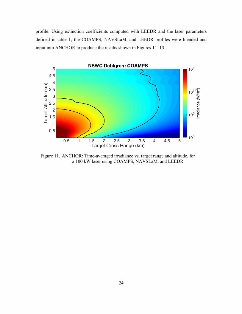
24
profile. Using extinction coefficients computed with LEEDR and the laser parameters
defined in table 1, the COAMPS, NAVSLaM, and LEEDR profiles were blended and
input into ANCHOR to produce the results shown in Figures 11–13.
Figure 11. ANCHOR: Time-averaged irradiance vs. target range and altitude, for a 100 kW laser using COAMPS, NAVSLaM, and LEEDR

25
Figure 12. ANCHOR: Power-in-the-bucket vs. target range and altitude for a 100 kW laser, using COAMPS, NAVSLaM, and LEEDR
Figure 13. ANCHOR: Required dwell time vs. target range and altitude for a 100 kW laser, using COAMPS, NAVSLaM, and LEEDR

26
In each of the figures, a figure of merit is plotted against target range and altitude
with the laser platform at the origin. The contour lines in Figure 11 represent threshold
values of 10 MW/m2 (contour closest to platform), 5 MW/m2, and 1 MW/m2 (contour
furthest from platform). The contour lines pull in toward the platform at low altitudes due
to high turbulence at the surface. The contour line in Figure 12 represents a power-in-the-
bucket threshold of 50 kW, and appears to decrease rapidly in the horizontal direction at
low altitude. Figure 13 shows the required dwell time plot with the dwell time threshold,
5 s, denoted by the black contour line. Figure 13 also shows that the required dwell time
diverges beyond a range of 1 km at the surface due to the high turbulence.
Using the blend of COAMPS, NAVSLaM, and LEEDR for the atmospheric input
into ANCHOR allows the operator to calculate a laser’s effectiveness in near-real time,
creating a more realistic assessment of operational employment.

27
IV. THERMAL BLOOMING
A. THERMAL BLOOMING OVERVIEW
Along the transmission path of a laser beam, the laser propagates through various
absorbing media. As the beam passes through the media, thermal energy is transferred
from the beam to the air, causing the air to heat up. This alters the air’s density and
therefore its index of refraction. These fluctuations cause the beam to spread out and
distort [13]. Figure 14 highlights the effects of thermal blooming on the laser beam. The
white contour represents 1/e of the peak irradiance. The left portion of the figure—the
side view of the beam—shows the thermal blooming induced beam spreading after
passing through an absorbing medium represented by a diverging lens denoted by the
black line. The right portion of the figure is the transverse profile of the beam and shows
that the effects of thermal blooming are most pronounced at the center of the beam,
where a donut-shaped intensity pattern appears, due to the diverging lens.
Figure 14. Laser diffraction simulation highlighting thermal blooming effects in the atmosphere
Understanding thermal blooming is important in calculating the time-averaged
irradiance when studying laser weapons systems. The effects of thermal blooming
become more pronounced at higher laser powers, especially in the maritime environment
where there is generally higher absorption. Beyond a certain threshold power level, the
thermal blooming becomes so severe that increasing the laser power will decrease the
irradiance on target, potentially affecting the range of the laser.
28
B. THERMAL BLOOMING THEORY
The diffraction of a laser along its propagation path is described by the paraxial
wave equation:
, (12)
where the irradiance is given by:
. (13)
Here, is the speed of light in a vacuum, is the permittivity of a vacuum, and is the
complex laser field. Equation 12 incorporates the effects due to extinction, ; the
effects due to diffraction, ; and the effects due to turbulence and thermal
blooming, .
The component, where , includes the changes in the
refractive index from both turbulence and thermal blooming [13]. The thermal blooming
contribution represents the change in the refractive index caused by the change in
temperature of the air due to thermal blooming:
. (14)
Here, no represents the initial index of refraction for the atmosphere and is calculated
using the isobaric heating equation:
. (15)
Here, includes the effects due to laser heating, where is the atmospheric
absorption coefficient, is the air density, and is the specific heat at constant
pressure. The term includes the effects due to convective heat transfer, where
is the wind velocity and is the transverse Laplacian. Essentially, the term
∂ψ∂z
= − ε2ψ + i
2k∇⊥2ψ + ikδn( )ψ
I = cεo2ψ ∗ψ
c εo ψ
− ε2ψ
i2k
∇⊥2ψ
ikδn( )ψ
δn δn = δnTB +δnTurb
δnTB n
ΔT
δnTB =dndT
ΔT = − no −1T
ΔT
ΔT
∂ΔT∂t
= αρCp
I − !v i!∇⊥( )ΔT + K
ρCp
∇2⎛
⎝⎜⎞
⎠⎟ΔT
αρCp
I α
ρ Cp
!v i!∇⊥( )ΔT
!v
!∇⊥
!v i!∇⊥

29
picks off the components of the wind velocity that are perpendicular to the beam path.
The term includes the effects due to conductive heat transfer; typically, the
effects due to conduction are much smaller than those due to convection and can be
ignored [14]. From Equation 15 it is important to note that depends on (which is
what we are trying to find) and depends on (and, consequently, on ). Therefore,
in order to solve for and , full diffraction codes solve Equations 12 and 15
numerically and iteratively along the beam path.
Deriving a numerical solution to these equations is time intensive, generally
taking a full diffraction code minutes to hours to solve. In order to attain a solution in a
fraction of the time, scaling codes typically fit a curve to the output from numerical
diffraction codes. The form of the curve fit is usually:
, (16)
where, STB is the thermal blooming Strehl ratio discussed in the previous chapter, A and B
are the fitting coefficients and ND is the thermal blooming distortion number defined as:
. (17)
Here, P is the laser power, z is along the path of the laser, nT = dn dt = − no −1( ) To , v is
the transverse wind speed, and D is the diameter of the beam. One of the issues with
using ND is that it is dependent upon the beam diameter, which itself depends on thermal
blooming.
ANCHOR, a scaling code, uses a similar method to calculate the thermal
blooming Strehl ratio, :
STB =1
1+ ANcsw
B NFC , (18)
where A, B, and C are fitting coefficients; Ncsw is the weighted collimated distortion
number defined as follows:
KρCp
∇2⎛
⎝⎜⎞
⎠⎟ΔT
ΔT I
I δn ΔT
I ΔT
STB =1
1+ ANDB
ND = − 4 2kPρCp
α z( )T z( )nT z( )v z( )D z( )∫ dz
STB

30
Ncsw = Nc z( )W z( )z∑ , (19)
where W is a weighting function, z is the path coordinate, and Nc is the collimated
distortion number defined as follows:
Nc z( ) = no −1( )α z( )Pz2πnoρCpT z( )v z( )Do
3 . (20)
Here, Do is the beam diameter at the source. Because the effects of thermal blooming
vary based upon where along the path the measurement is taken and upon the size of the
beam diameter – peak thermal blooming tends to occur closer to the platform for smaller
diameters – it is beneficial to multiply Nc by a weighting function given in [15]. The
Fresnel number is derived from the following equation:
. (21)
Here, is the beam radius at the source and is defined as the spot size radius
including only the effects of diffraction as defined in equations 7 and 8 from the previous
chapter, short-term turbulence as discussed below, and jitter as discussed in the previous
chapter. In weak turbulence, ro > Do 3 , where ro is the Fried parameter, the contribution
due to short-term turbulence is given by [8]:
wts = 0.182 wd
M 2⎛⎝⎜
⎞⎠⎟
Do
ro
⎛⎝⎜
⎞⎠⎟
. (22)
For stronger turbulence, when ro < Do 3 , the following equation is used:
wts =wd
M 2Do
ro
⎛⎝⎜
⎞⎠⎟
2
−1.18 Do
ro
⎛⎝⎜
⎞⎠⎟
53
. (23)
Because the beam wandering effects of long-term turbulence happen on a longer time-
scale than the development of thermal blooming effects, the long-term turbulence
contribution can be ignored when calculating thermal blooming. By replacing the total
turbulence term, with short-term turbulence in the spot radius equation from the
previous chapter, can be calculated. Including NF allows ANCHOR to account for
the first order effects caused by turbulence, diffraction, and jitter into the Strehl ratio for a
more physical representation of thermal blooming.
NF =Rowtots
Ro wtots
wt
wtots

31
C. THERMAL BLOOMING CALIBRATION
TBWaveCalc, a script-driven atmospheric propagation tool, was used to
determine the A, B, and C coefficients for the Strehl ratio from equation 18. TBWaveCalc
is built into ATMTools and is developed by MZA. It is a full diffraction code that can
model the path of a laser beam given the initial laser geometry and atmospheric
conditions, and includes thermal blooming and combined turbulence effects [16].
In order to calibrate ANCHOR’s thermal blooming Strehl ratio, TBWaveCalc was
run for several thousand different laser and atmospheric parameters, consuming many
thousands of hours of computer processing time. A MATLAB script was developed to
generate the TBWaveCalc input files, analyze the output, and calculate Nc, Ncsw, and NF.
The laser and atmospheric parameters were chosen to cover a wide variety of initial
conditions and output powers. TBWaveCalc was run multiple times for a given
atmosphere and laser geometry using different random seeds for the turbulence screens,
and then the results were averaged.
The TBWaveCalc Strehl ratio was calculated from the ratio of peak irradiances
after running the code with and without thermal blooming. The ANCHOR Strehl ratio
was calculated using Equation 18 for the Ncsw and NF values obtained from MATLAB.
Initial guesses for coefficients A, B, and C were used to calculate the initial value for the
ANCHOR Strehl ratio. From the initial Strehl ratio, the inverse Strehl ratio was
calculated and compared against the inverse Strehl ratio calculated from the
TBWaveCalc results. The difference between the inverse Strehl ratios were tabulated in
Excel and then summed together. The sum of differences was then input into the Excel
solver function where, the A, B, and C coefficients were adjusted in order to minimize the
sum of the differences. These coefficients were then incorporated into Equation 18 in
order to calculate the “best fit” Strehl ratio for ANCHOR. The ANCHOR Strehl ratio was
then plotted against the thermal blooming Strehl ratio calculated from TBWaveCalc and
compared, as shown in Figures 15–43.

32
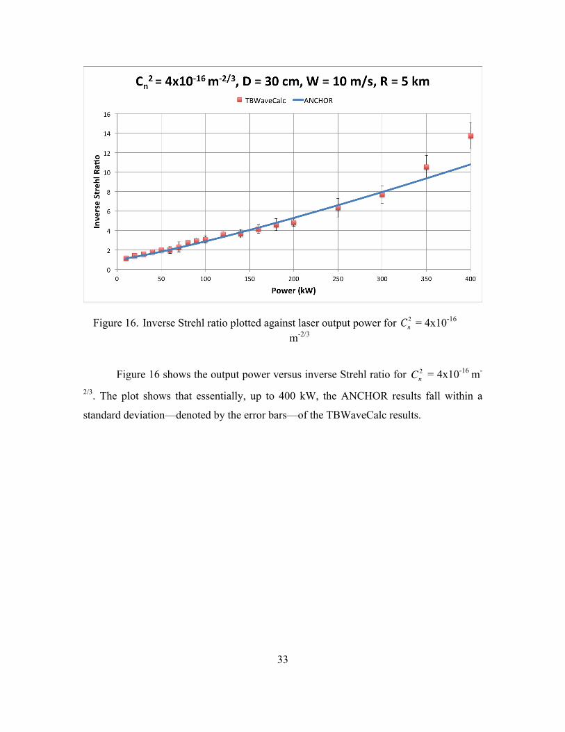
1. Results: Wind = 10 m/s, D = 30 cm, Range = 5 km
In order to see how ANCHOR’s calibrated thermal blooming model compares to
TBWaveCalc, the inverse Strehl ratios were plotted against each other for a variety of
conditions. Since the Strehl ratio is a value between 0 and 1, the inverse Strehl ratio was
plotted instead. Plotting the inverse Strehl ratios versus output power elucidates small
differences between the results for strong thermal blooming, i.e., when . In
Figures 15–21, the inverse Strehl ratio is plotted against output laser power from 10 kW
to 400 kW. The beam diameter at the source is 30 cm, the wind is a constant 10 m/s, and
the range is 5 km. The blue line represents the ANCHOR data and the red points
represent TBWaveCalc results.
Figure 15. Inverse Strehl ratio plotted against laser output power for Cn2 = 0
Figure 15 shows output power versus inverse Strehl ratio for = 0 (i.e., no
turbulence). The plot shows that at low powers ANCHOR and TBWaveCalc compare
well; however, at higher powers the variation is more noticeable with about a 30%
difference.
STB ≪1
Cn2
33
Figure 16. Inverse Strehl ratio plotted against laser output power for Cn2 = 4x10-16
m-2/3
Figure 16 shows the output power versus inverse Strehl ratio for = 4x10-16 m-
2/3. The plot shows that essentially, up to 400 kW, the ANCHOR results fall within a
standard deviation—denoted by the error bars—of the TBWaveCalc results.
Cn2

34
Figure 17. Inverse Strehl ratio plotted against laser output power for Cn2 = 8x10-16
m-2/3
Figure 18. Inverse Strehl ratio plotted against laser output power for Cn2 = 4x10-15
m-2/3
35
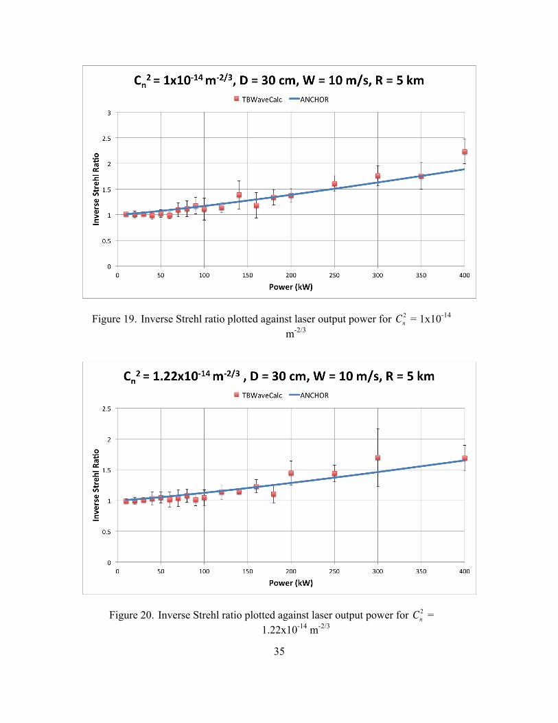
Figure 19. Inverse Strehl ratio plotted against laser output power for Cn2 = 1x10-14
m-2/3
Figure 20. Inverse Strehl ratio plotted against laser output power for Cn2 =
1.22x10⁻¹⁴ m-2/3

36
Figure 21. Inverse Strehl ratio plotted against laser output power for Cn2 = 2x10-14
m-2/3
Figures 15–21 show output power versus inverse Strehl ratio for increasing
turbulence in ascending order. At the power levels shown, these plots continue to show
that the ANCHOR results compare well with TBWaveCalc, with ANCHOR’s thermal
blooming model falling within a standard deviation of the TBWaveCalc results. Figure
21 only shows output power from 10 to 200 kW and shows that at lower power levels the
ANCHOR model agrees very well with TBWaveCalc. The general trend is that thermal
blooming has a decreasing effect as turbulence becomes stronger; this happens because
turbulence increases spot size, decreasing the irradiance.
2. Results: Wind = 10 m/s, D = 30 cm, Slant Range = 5 km
Figures 22 and 23, using the same parameters for beam diameter and wind speed,
compare the ANCHOR and TBWaveCalc results for a 5 km slant range where Cn2 varies
along the path as altitude increases.

37
Figure 22. Inverse Strehl ratio plotted against laser output power for Cn2 = 1.7x10-
15 m-2/3 at the surface and a target altitude of 100 m
Figure 23. Inverse Strehl ratio plotted against laser output power for Cn2 = 9x10-15
m-2/3 at the surface and a target altitude of 1000 m

38
The plot shown in Figure 22 for a slant range with Cn2 = 1.7x10⁻¹⁵ m-2/3 at the
surface and a target altitude of 100 m, shows that ANCHOR’s thermal blooming model is
in agreement with TBWaveCalc. Likewise, Figure 23 with a profile Cn2 = 9x10-15 m-2/3 at
the surface and a target altitude of 1000 m also shows good agreement between
ANCHOR and TBWaveCalc.
3. Results: Wind = 5 m/s, D = 30 cm, Range = 5 km
In Figures 24 and 25, the inverse Strehl ratio is plotted against output laser power
from 10 kW to 400 kW. The beam diameter at the source is 30 cm; the wind is a constant
5 m/s; the range is 5 km.
Figure 24. Inverse Strehl ratio plotted against laser output power for Cn2 = 4x10-16 m-2/3

39
Figure 25. Inverse Strehl ratio plotted against laser output power for Cn2 = 8x10-16 m-2/3
For a light wind of 5 m/s, the ANCHOR thermal blooming model agrees well
with TBWaveCalc for low powers but the deviation when turbulence is low is more
noticeable at high powers.
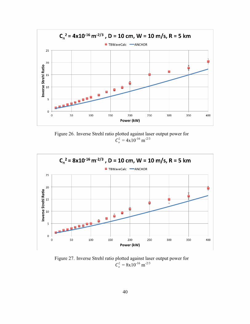
4. Results: Wind = 10 m/s, D = 10 cm, Range = 5 km
In Figures 26–29, the inverse Strehl ratio is plotted against output power from 10
kW to 400 kW. The beam diameter at the source is 10 cm; the wind is constant at 10 m/s;
the range is 5 km.
40
Figure 26. Inverse Strehl ratio plotted against laser output power for Cn2 = 4x10-16 m-2/3
Figure 27. Inverse Strehl ratio plotted against laser output power for Cn2 = 8x10-16 m-2/3

41
Figure 28. Inverse Strehl ratio plotted against laser output power for Cn2 = 4x10-15 m-2/3
Figure 29. Inverse Strehl ratio plotted against laser output power for Cn2 = 1x10-14 m-2/3

42
Figures 26–29 show that for a beam diameter at the source of 10 cm, ANCHOR
and TBWaveCalc results agree very well for higher turbulence. The figures also show
that for lower turbulence the ANCHOR results slightly underestimate the TBWaveCalc
results.
5. Results: Wind = 10 m/s, D = 50 cm, Range = 5 km
For Figures 30–32, the inverse Strehl ratio is plotted against output power for a
beam diameter of 50 cm, a constant wind of 10 m/s, and a range of 5 km.
Figure 30. Inverse Strehl ratio plotted against laser output power for Cn2 = 4x10-16 m-2/3

43
Figure 31. Inverse Strehl ratio plotted against laser output power for Cn2 = 8x10-16 m-2/3
Figure 32. Inverse Strehl ratio plotted against laser output power for Cn2 = 1x10-14 m-2/3

44
Figures 30–32 show that the ANCHOR thermal blooming and TBWaveCalc
results agree well for a beam diameter at the source of 50 cm in strong turbulence.
Comparing the results in weak turbulence show the greatest variation at higher powers.
6. Results: Wind = 10 m/s, D = 30 cm, Range = 8 km
In Figures 33 and 34 the inverse Strehl ratio is plotted against output power for a
beam diameter of 30 cm, a constant wind of 10 m/s, and a range of 8 km.
Figure 33. Inverse Strehl ratio plotted against laser output power for Cn2 = 8x10-16 m-2/3

45
Figure 34. Inverse Strehl ratio plotted against laser output power for Cn2 = 4x10-15 m-2/3
Figures 33 and 34 show that the ANCHOR model and the TBWaveCalc results
agree well for a range of 8 km, showing almost no variation for Cn2 = 4x10-15 m-2/3 and
good agreement within a standard deviation for Cn2 = 8x10-16 m-2/3.
7. Results: Wind = 5 m/s, D = 30 cm, Range = 8 km
In Figure 35, the inverse Strehl ratio is plotted against output power for a beam
diameter of 30 cm, a constant wind of 5 m/s, and a range of 8 km.

46
Figure 35. Inverse Strehl ratio plotted against laser output power for Cn2 = 8x10-16
m-2/3
Comparing Figure 35 with Figure 33 shows that for Cn2 = 8x10-16 m-2/3 the
ANCHOR model agrees better with the TBWaveCalc for a wind speed of 5 m/s and a
range of 8 km, with Figure 35 falling within one standard deviation of the TBWaveCalc
results.
8. Results: Wind = 5 m/s, D = 30 cm, Range = 1 km
For Figures 36–38, the inverse Strehl ratio is plotted against output power for a
beam diameter of 30 cm, a constant wind of 5 m/s, and a range of 1 km.

47
Figure 36. Inverse Strehl ratio plotted against laser output power for Cn2 = 8x10-16 m-2/3
Figure 37. Inverse Strehl ratio plotted against laser output power for Cn2 = 4x10-15 m-2/3
48
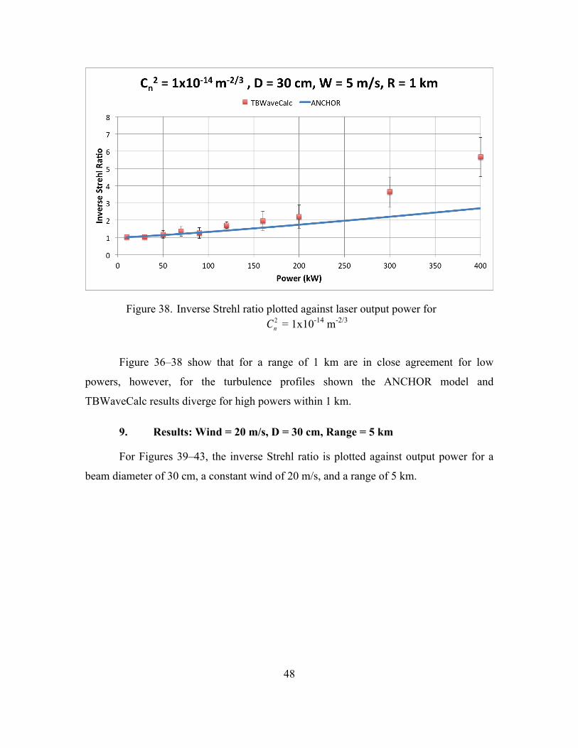
Figure 38. Inverse Strehl ratio plotted against laser output power for Cn2 = 1x10-14 m-2/3
Figure 36–38 show that for a range of 1 km are in close agreement for low
powers, however, for the turbulence profiles shown the ANCHOR model and
TBWaveCalc results diverge for high powers within 1 km.
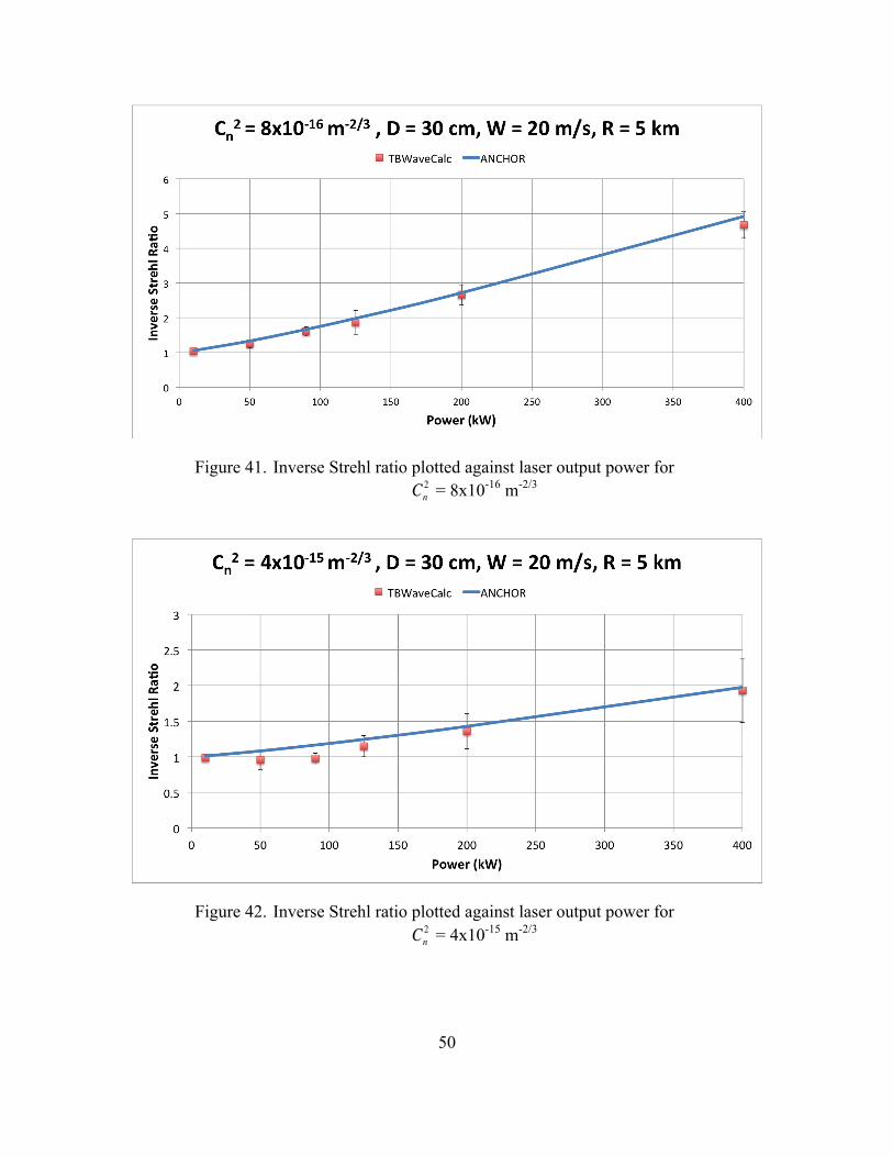
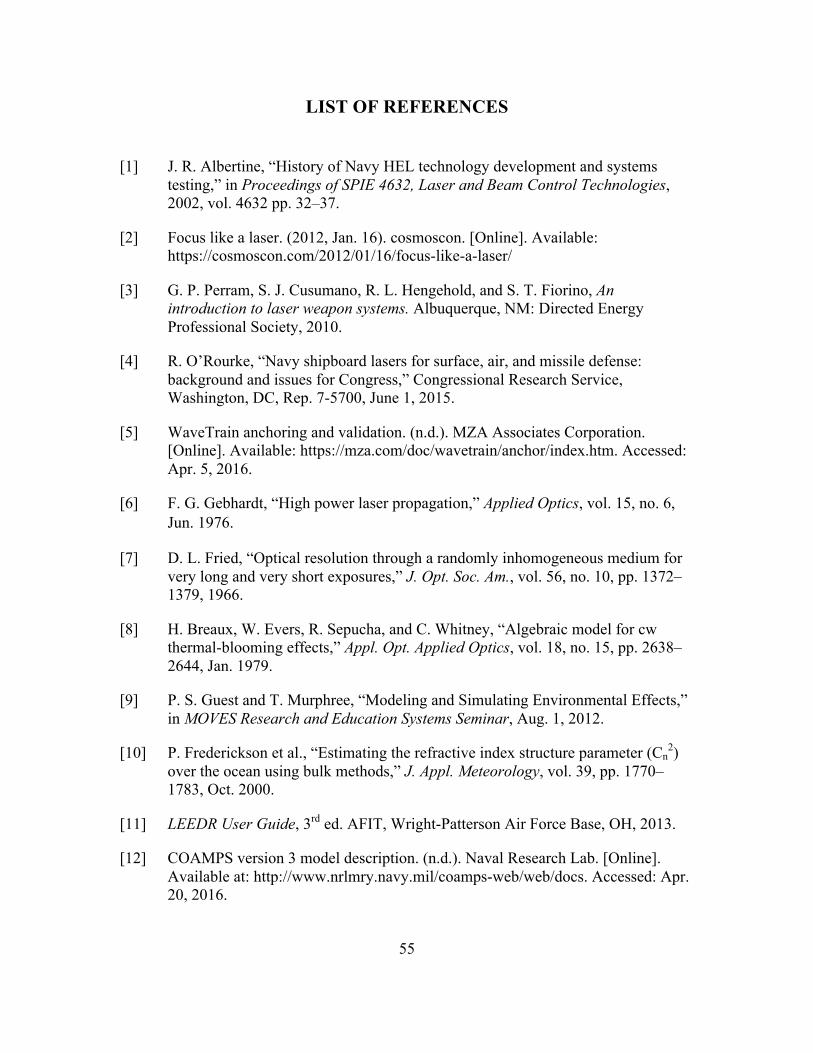
9. Results: Wind = 20 m/s, D = 30 cm, Range = 5 km
For Figures 39–43, the inverse Strehl ratio is plotted against output power for a
beam diameter of 30 cm, a constant wind of 20 m/s, and a range of 5 km.

49
Figure 39. Inverse Strehl ratio plotted against laser output power for Cn2 = 0
Figure 40. Inverse Strehl ratio plotted against laser output power for Cn2 = 4x10-16 m-2/3
50
Figure 41. Inverse Strehl ratio plotted against laser output power for Cn2 = 8x10-16 m-2/3
Figure 42. Inverse Strehl ratio plotted against laser output power for Cn2 = 4x10-15 m-2/3

51
Figure 43. Inverse Strehl ratio plotted against laser output power for Cn2 = 1x10-14
m-2/3
Figures 39–43 show that for a constant wind speed of 20 m/s the ANCHOR
model and TBWaveCalc results continue to agree well at higher turbulence with larger
variation occurring at lower turbulence at higher power levels.

52
THIS PAGE INTENTIONALLY LEFT BLANK

53
V. CONCLUSION
The focus of this thesis was the calibration of the ANCHOR thermal blooming
model against TBWaveCalc in a variety of conditions for laser output powers from 10
kW to 400 kW. The results of that calibration, illustrated in the previous chapter, show
that the ANCHOR model, which uses a simple analytical scaling formula, is in general
agreement with most of the TBWaveCalc results after adjusting the coefficients of the
scaling formula. The results also show that the correlation is particularly strong at lower
output powers, however, showing noticeable deviations in the 300–400 kW range for
smaller turbulence values. Deviation was also noted for lower wind velocities, as the
differences at high powers increased markedly as wind velocity decreased from 10 m/s to
5 m/s. For higher turbulence values, ANCHOR and TBWaveCalc show good correlation
across the results with the exception of the 1 km range. Overall, the updated ANCHOR
thermal blooming model shows good agreement with TBWaveCalc.
More work can be done to further refine the ANCHOR thermal blooming model.
Future work includes increasing the data set of TBWaveCalc results for better correlation
with ANCHOR. Future projects can also be done in order to calibrate the ANCHOR
thermal blooming model for a Gaussian profile.

54
THIS PAGE INTENTIONALLY LEFT BLANK
55
LIST OF REFERENCES
[1] J. R. Albertine, “History of Navy HEL technology development and systems testing,” in Proceedings of SPIE 4632, Laser and Beam Control Technologies, 2002, vol. 4632 pp. 32–37.
[2] Focus like a laser. (2012, Jan. 16). cosmoscon. [Online]. Available: https://cosmoscon.com/2012/01/16/focus-like-a-laser/
[3] G. P. Perram, S. J. Cusumano, R. L. Hengehold, and S. T. Fiorino, An introduction to laser weapon systems. Albuquerque, NM: Directed Energy Professional Society, 2010.
[4] R. O’Rourke, “Navy shipboard lasers for surface, air, and missile defense: background and issues for Congress,” Congressional Research Service, Washington, DC, Rep. 7-5700, June 1, 2015.
[5] WaveTrain anchoring and validation. (n.d.). MZA Associates Corporation. [Online]. Available: https://mza.com/doc/wavetrain/anchor/index.htm. Accessed: Apr. 5, 2016.
[6] F. G. Gebhardt, “High power laser propagation,” Applied Optics, vol. 15, no. 6, Jun. 1976.
[7] D. L. Fried, “Optical resolution through a randomly inhomogeneous medium for very long and very short exposures,” J. Opt. Soc. Am., vol. 56, no. 10, pp. 1372–1379, 1966.
[8] H. Breaux, W. Evers, R. Sepucha, and C. Whitney, “Algebraic model for cw thermal-blooming effects,” Appl. Opt. Applied Optics, vol. 18, no. 15, pp. 2638–2644, Jan. 1979.
[9] P. S. Guest and T. Murphree, “Modeling and Simulating Environmental Effects,” in MOVES Research and Education Systems Seminar, Aug. 1, 2012.
[10] P. Frederickson et al., “Estimating the refractive index structure parameter (Cn2)
over the ocean using bulk methods,” J. Appl. Meteorology, vol. 39, pp. 1770–1783, Oct. 2000.
[11] LEEDR User Guide, 3rd ed. AFIT, Wright-Patterson Air Force Base, OH, 2013.
[12] COAMPS version 3 model description. (n.d.). Naval Research Lab. [Online]. Available at: http://www.nrlmry.navy.mil/coamps-web/web/docs. Accessed: Apr. 20, 2016.

56
[13] F. Zhang, and Y Li, “The scaling laws for thermal blooming of the high-energy laser propagation,” in Proceedings of SPIE 5832 Optical Technologies for Atmospheric, Ocean, and Environmental Studies, 2005, vol. 5832 pp. 25-30.
[14] F. G. Gebhardt, “Twenty-five years of thermal blooming: An overview,” in Proceedings of SPIE 1221 Propagation of High-Energy Laser Beams Through the Earth’s Atmosphere, 1990, vol. 1221 pp. 2-25.
[15] A. M. Ngwele and M. R. Whiteley, “Scaling law modeling of thermal blooming in wave optics,” in DEPS Directed Energy Symposium, Nov. 2, 2006.
[16] E.P. Magee and A.M. Ngwele. (2013). ATMTools: A toolbox for atmospheric propagation modeling [Online]. Available: http://scalingcodes.mza.com/doc/AtmToolsUserGuide.pdf

57
INITIAL DISTRIBUTION LIST
1. Defense Technical Information Center Ft. Belvoir, Virginia 2. Dudley Knox Library Naval Postgraduate School Monterey, California