1

Adaptation Strategies on Flexible Pavement Design Practices Due to Climate Change in

Canada

Paula Sutherland Rolim Barbi

Ph.D. Candidate

University of Waterloo

Guangyuan Zhao

Research Associate

University of Waterloo

Seyedata Nahidi

Research Associate

University of Waterloo

Jessica Achebe

Ph.D. Candidate

University of Waterloo

Susan Tighe

Provost and Vice-President, Academic

McMaster University

Paper prepared for Innovations in Pavement Management, Engineering and Technologies

session of the 2021 TAC Conference & Exhibition

2

Abstract

It has been shown that Canada’s climate is warming at more than double the global rate [1],

therefore, Canadian road infrastructure could be at risk if adaptation strategies are neglected.

Key climatic parameters that govern the design and performance of flexible pavement may alter

in the future, leading to different climatic loads on road structures, which in turn may result in

reduced performance and shortened service life. To that end, this research aims to propose a

methodology for the incorporation of climatic projected changes in the design of flexible

pavement in Canada. To reach this goal, first, climate change projections over Canada will be

evaluated and limitations of existing climatic data used for pavement structural design will be

assessed; second, the impacts of climate change on pavement performance will be further

discussed, followed by the introduction of a methodology to incorporate climate change

predictions in pavement structural design; lastly, an example will be performed to illustrate the

incorporation of the climate change parameters in the design procedure of AASHTO 93. The

climatic inputs to be evaluated are temperature, precipitation, permafrost thawing, and freeze-

thaw cycles. This study aims not only to provide guidelines for flexible pavement design but also

to raise public awareness by engaging government and stakeholders across the country.

Introduction

The 2019 Climate Change Report – CCCR2019 developed by the Government of Canada

shows that Canada’s climate is warming at more than double the global rate [1]. It is anticipated

that heat waves will occur more often and last longer and that the potential rutting will increase

with higher extreme in-service pavement temperatures [2]. Extreme precipitation events in many

regions are more severe and frequent, which will lead to flood damage. At the same time, road

structures will freeze later but thaw sooner with correspondingly shorter freezing periods in the

evolving environments.

Road infrastructure is essential to the Canadian economy, as most goods and services are

transported primarily by trucks and cars. These roads are highly vulnerable as they were not

designed to tackle the changing climate conditions adequately. The concerns related to the

changing climate in pavement design and management include reduced performance, loss of

serviceability, shortened service life, more frequent maintenance and rehabilitation, higher

construction and operation costs, and adverse socio-economic impacts on communities [3], [4],

[5]. A comprehensive understanding of the effects of climate change on road infrastructure is,

therefore, vital for decision-making that takes climate risks into account and improves adaptive

planning.

In Canada, flexible pavement design methods vary in different provinces. In recent years, the

Mechanistic-Empirical Pavement Design Guide (MEPDG) is becoming more common, however,

the most common design method in Canada is still the 1993 AASHTO Guide for Design of

Pavement Structures [5]. In the AASHTO 93 method, the climatic factors are not always used as

a direct design input, however, the consideration of the climatic factors could be incorporated

when selecting design inputs related to pavement materials and performance criteria. To that

end, this research aims to propose a methodology for the incorporation of climatic projected

changes in the design of flexible pavement in Canada. This methodology can be used as a

guide for pavement designers in Canada to consider climate change in their practices.

3

Climate Projections in Canada

Temperature

In 2019, a detailed report concerning the temperature changes in Canada was published by

Environment and Climate Change Canada. This report presented several crucial facts which

later could affect the life cycle of the infrastructures and specifically pavements and roads.

Based on this report, by analyzing the temperature data between 1948 to 2019, it can be

concluded that the annual average temperature increased by 1.7ºC.

It was also reported that the average spring and autumn temperature increased by 1.7ºC from

1948 to 2019. Moreover, throughout the very same timeframe, winters got warmer by 3.3ºC.

The least change in seasonal average temperature was for summer with 1.4ºC increase. The

most changes in regional temperature were recorded in northern provinces and territories such

as Yukon, Northwest Territories, and Nunavut. These changes can significantly reduce the

thickness of glaciers, increase the sea levels and significantly endanger species [1].

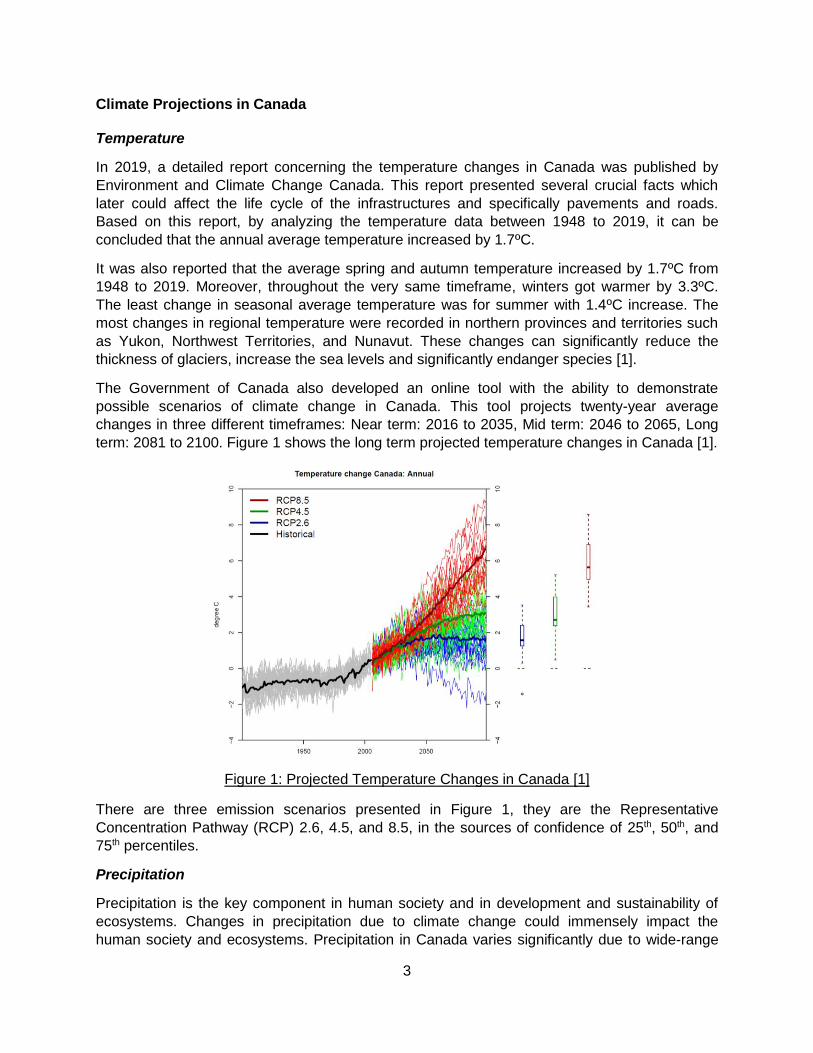
The Government of Canada also developed an online tool with the ability to demonstrate

possible scenarios of climate change in Canada. This tool projects twenty-year average

changes in three different timeframes: Near term: 2016 to 2035, Mid term: 2046 to 2065, Long

term: 2081 to 2100. Figure 1 shows the long term projected temperature changes in Canada [1].

Figure 1: Projected Temperature Changes in Canada [1]

There are three emission scenarios presented in Figure 1, they are the Representative

Concentration Pathway (RCP) 2.6, 4.5, and 8.5, in the sources of confidence of 25th, 50th, and

75th percentiles.

Precipitation

Precipitation is the key component in human society and in development and sustainability of

ecosystems. Changes in precipitation due to climate change could immensely impact the

human society and ecosystems. Precipitation in Canada varies significantly due to wide-range

4

of temperature and diverse topography, resulting in annual precipitations that goes from more

than 3000 mm to less than 200 mm in some areas [6].

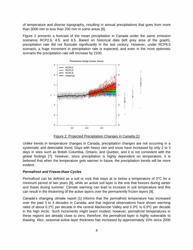
Figure 2 presents a forecast of the mean precipitation in Canada under the same emission

scenarios RCP2.6, 4.5, and 8.5. Based on historical data (left grey area of the graph),

precipitation rate did not fluctuate significantly in the last century. However, under RCP8.5

scenario, a huge increment in precipitation rate is expected, and even in the most optimistic

scenario the precipitation rate will increase by 2100.

Figure 2: Projected Precipitation Changes in Canada [1]

Unlike trends in temperature changes in Canada, precipitation changes are not occurring in a

systematic and detectable trend. Days with heavy rain and snow have increased by only 2 to 3

days in sites such as British Columbia, Ontario, and Quebec, and it is not consistent with the

global findings [7]. However, since precipitation is highly dependent on temperature, it is

believed that when the temperature gets warmer in future, the precipitation trends will be more

evident.

Permafrost and Freeze-thaw Cycles

Permafrost can be defined as a soil or rock that stays at or below a temperature of 0°C for a

minimum period of two years [8], while an active soil layer is the one that freezes during winter

and thaws during summer. Climate warming can lead to increase in soil temperature and this

can result in the thickening of the active layers over the permanently frozen layers [9].

Canada’s changing climate report [1] informs that the permafrost temperature has increased

over the past 3 to 4 decades in Canada, and that regional observations have shown warming

rates of about 0.1ºC per decade in the central Mackenzie Valley and 0.3ºC to 0.5ºC per decade

in the high Arctic. Such increments might seem modest, however, permafrost temperatures in

these regions are already close to zero, therefore, the permafrost layer is highly vulnerable to

thawing. Also, seasonal active layer thickness has increased by approximately 10% since 2000

5

in the Mackenzie Valley, making those areas more prone to deformations caused by freeze-

thaw cycling.

The CCCR2019 report [1] also indicates some climate models that project large increments in

the surface temperature across permafrost areas in Canada, which could result in a total

increase of over 8°C in the mean surface temperature by the end of the 21st century. However,

while air temperature predictions can be quite accurate, it is challenging to project associated

reductions in permafrost extent from climate model simulations, because of unknown soil

properties and ice content, and other uncertainties regarding the response of deep layers of

permafrost (which can exceed hundreds of meters below surface).

There are several models simulating future reduction in permafrost extent, some being more

pessimistic than others. For example, Kettles estimated that permafrost areas in Canada could

be reduced by 43% under a 2°C to 5°C warming scenario [10], while Lawrence and Slater

predicted that 90% of the near‐surface permafrost in the Northern Hemisphere can disappear in

the next 80 years [11]. However, a study developed by Zhang predicts a narrower range of

permafrost reduction, from 20.5% to 24.4%, compared to air temperature increase from 2.8 to

7.0°C [12].

With the shortening of the freezing season due to climate change, locations where pavement

layers have long frozen periods, such as the discontinuous permafrost areas, will likely suffer

with more freezing and thawing cycles, and that might increase frost heave and differential thaw

settlement. Another effect of the warming trend is that in southern areas of Canada, it is

expected that pavement will suffer less with frost heave since frost penetration depth will

decrease due to the shortening of the winter season [13].

Impact of Climate Change on Pavement Performance

Temperature

Temperature as one of the most important components of the climate change factors plays a

significant role on the performance of the flexible pavement. Higher pavement layer temperature

can reduce the stiffness of asphalt materials and interrupt the proper spread of loads [14].

Moreover, increasing temperature due to climate change can accelerate the pavement ageing

and development of cracks. Temperature can also indirectly affect the resilient modulus of

granular layers and subgrade, since it will dictate when the water embedded in those materials

is frozen or not, therefore, the seasonal resilient moduli of unbonded materials can vary

according to both temperature and moisture conditions.

Precipitation

The moisture content of the flexible pavements is generally impacted by the precipitation and

groundwater. Generally, moisture affects the flexible pavement by reducing the adhesion

between binder and aggregates and initiating distresses such as stripping [15], [16]. Also,

excessive moisture can cause a perceptible reduction in resilient modulus of unbound and

subgrade materials [17]. Since ample moisture reduces the shear strength of the unbound and

subgrade materials, it is expected to observe permanent deformation, rutting, and even failure

of the flexible pavements under excessive precipitation [18], [19]. Studies also showed that

flexible pavements with more fine aggregates are more likely to experience severe moisture

6

damages [17]. In AASHTO 93 design method, some of the variables that can account for the

effect of higher soil moisture are the serviceability loss, soil resilient modulus, layer coefficients

and drainage.

Some studies have correlated groundwater levels with precipitation and determined that the two

variables tend to mirror each other with a delay [20], however, groundwater level trends are

difficult to predict, due their complexity within the Canadian landscape and due to human

withdrawals. One alternative could be to monitor the available data from provincial wells and

look for local trends near the project site.

Permafrost and Freeze-thaw Cycles Impacts

The thawing of previously permanent frozen layers can cause serious damage to pavement

structures. Settlement caused by thawing starts with a change in soil volume followed by a

subsequent consolidation, in which the loads applied are transferred from the pore water to the

soil skeleton. The degree of settlement will highly depend on the type of soil, density, pore water

pressure generated and the soil’s ability to compress. Subgrades rich in fine particles such as

silt and clay, with access to capillary water, will usually present large settlements when loaded

[21].

When a pavement reaches freezing conditions, the water trapped in the pavement will naturally

freeze and expand. Therefore, heave can be identified as the upward displacement of the soil

surface, led by transport processes under the surface as freezing occurs [22]. Certain types of

soils can be more prone to heave, for example, silts and clays can produce very prominent

heave, while sands and gravels not so much. Another factor that plays an important role is the

groundwater table. Higher groundwater table levels can be correlated with greater frost heave

damage.

Considering that one of the more severe climate change deterioration mechanisms can be

attributed to freeze-thaw (FT) cycles, the increase in this event should be considered when

designing and restoring pavements. One FT cycle can be considered as the fluctuation of the

pavement’s temperature, from above freezing to below freezing and then back to above

freezing, and it can degrade the pavement structure through a few mechanisms, explained

below.

First, when the weather reaches negative temperatures, the water trapped into the AC cracks

and voids can freeze, expanding and damaging the aggregates and binder. This can cause

stripping and raveling due to the loss of bond between aggregates in the asphalt concrete layer.

Next, when temperature rises to positive, the water will melt and penetrate the unbonded layers.

When the cycle starts over, the water that moved to the granular layers or subgrade will freeze

again, possibly causing frost heave and depressions when melted.

Because the freeze-thaw cycle weakens the bond between aggregates in the asphalt concrete,

it can also induce the asphalt mix to become softer, making it more susceptible to rutting and

shoving [23]. Studies showed that the number of FT cycles can decrease the Marshall Stability

by 77.4% after 24 days of cycles [24] and they can also cause a drastic decrease in tensile

strength ratio when samples were subjected to a repeated number of cycles [25]. For a regular

AC mix, rutting can be up to three times higher after 50 cycles of freezing and thawing,

however, polymer modified mixes have presented a very positive performance under the FT

cycles [26].

7

Even though there are a variety of studies relating FT cycles and damage mechanisms, there is

no closed equation that relates the number of cycles and the decrease in the resilient modulus

or any other stiffness measurement. Therefore, it is not yet possible to assertively predict the

stiffness loss of asphalt concrete pavements under freezing and thawing cycles yet, since more

research must be done in this field.

In AASHTO 93, the climatic region is not a direct structural design factor, but it can be very

useful to provide information such as the frequency of the freeze-thaw cycle, the susceptibility of

soil swelling, and moisture level from precipitation. With this information, frost heaving and soil

swelling may be treated with a better drainage system or reflected in serviceability loss. The

climatic region is also helpful in determining the proper pavement materials. For example, the

asphalt concrete mix design can be improved by selecting the appropriate binder grade and

aggregate source, but this part is not directly contained in the pavement structural design.

Lastly, the serviceability loss should account for environmental impacts caused by frost heave

and roadbed swelling, therefore, the increase in the number of FT cycles could also be

incorporated in this variable.

Designers who follow the AASHTO 93 guide may not be aware that some material properties or

pavement characteristics must be reselected or adjusted due to climate change. Without

considering the impact of climate change on climate-related design inputs, the pavement may

not meet performance expectations, resulting in more frequent maintenance and rehabilitation,

early failure, and great economic losses.

Incorporation of Climate Change Predictions in Pavement Structural Design

Drainage Coefficients

The drainage level is considered in AASHTO 93 by introducing the drainage coefficients (mi) in

modifying the layer coefficient for the base and subbase courses and calculating the final

Structural Number (SN) value. The mi values are a function of the quality of drainage and

percent of the time pavement structure is exposed to moisture levels. The percent of time

pavement structure is exposed to moisture levels is affected by the average yearly rainfall and

the prevailing drainage conditions. The recommended drainage coefficients for flexible

pavement are provided in Table 1.

During the design process, it is up to the designers to determine the drainage level. When the

impacts of future climate conditions are considered in the drainage design section, the drainage

quality assumption must be made first, followed by selecting the exposure to moisture based on

the average yearly rainfall and assumed prevailing drainage conditions [27].

8

Table 1: Recommended Drainage Coefficients (mi) for Flexible Pavements [5]

Percent of Time Pavement Structure is Exposed to Moisture Levels Approaching Saturation

Quality of Drainage

< 1% 1-5% 5-25% > 25%

Excellent 1.40-1.35 1.35-1.30 1.30-1.20 1.20

Good 1.35-1.25 1.25-1.15 1.15-1.00 1.00

Fair 1.25-1.15 1.15-1.05 1.00-0.80 0.80

Poor 1.15-1.05 1.05-0.80 0.80-0.60 0.60

Very Poor 1.05-0.95 0.95-0.75 0.75-0.40 0.40

Soil Resilient Modulus

One of the common methods to evaluate the stiffness of the unbound pavement materials is the

resilient modulus (MR). The Federal Highway Administration (FHWA) defines this factor as “the

ratio of the applied cyclic stress to the recoverable (elastic) strain after many cycles of repeated

loading”. Besides direct laboratory tests, the MR value can be derived from various methods and

techniques, such as the R-value and CBR [5]. AASHTO 93 considers the seasonal effects on

the resilient modulus through relative damage as presented in Equation 1.

𝑢𝑓 = 1.18 ∗ 108 ∗ 𝑀𝑅−2.32 Equation 1

In which, 𝑢𝑓 is the relative damage for a given modulus and 𝑀𝑅 is the resilient modulus for a

time period. Relative damages per month or per season can be yearly averaged and re-

converted to 𝑀𝑅 to produce the effective resilient modulus of a subgrade. This effective resilient

modulus will then be used as an input for the pavement design.

Climate change can influence the soil resilient modulus through two main mechanisms: first, the

warming temperatures due to climate change will shorten frozen periods. Secondly, the thawing

phase can be more severe since the increase in precipitation levels could enhance soil

saturation and decrease soil resistance. Therefore, when computing relative damage, 𝑢𝑓, the

monthly or seasonally resilient modulus needs to be carefully estimated.

The groundwater table depth can vary significantly due to pumping of wells, evapotranspiration,

and rainfall [28]. Monitoring wells are present all over Canada, for example, information on

various collecting points can be found in the Provincial Groundwater Monitoring Network

(PGMN) program, available at the Government of Ontario website. Mass volume parameters

also play a decisive role in the modulus of a soil. The initial degree of saturation, 𝑆𝑜𝑝𝑡, optimum

volumetric water content, 𝜃𝑜𝑝𝑡, and saturated volumetric water content, 𝜃𝑠𝑎𝑡 can be either

obtained by direct laboratory tests, or through the gradation and engineering index properties.

The degree of soil moisture can also be called degree of saturation. During construction, the

degree of saturation is usually under optimum conditions, however after some time, the degree

of saturation tends to reach an equilibrium. This equilibrium degree of saturations is highly

influenced by the groundwater table depth, 𝑦𝐺𝑊𝑇, and the soil-water characteristic curve,

SWCC.

Depending on the temperature and moisture conditions, the soil can have degrees of saturation

different than the equilibrium state, however, the soil will always tend to go back to equilibrium

9

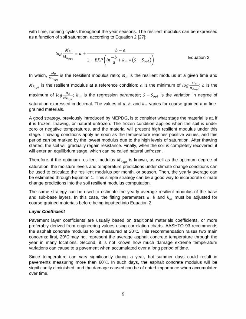
with time, running cycles throughout the year seasons. The resilient modulus can be expressed

as a function of soil saturation, according to Equation 2 [27]:

𝑙𝑜𝑔𝑀𝑅

𝑀𝑅𝑜𝑝𝑡

= 𝑎 +𝑏 − 𝑎

1 + 𝐸𝑋𝑃 (𝑙𝑛−𝑏𝑎

+ 𝑘𝑚 ∗ (𝑆 − 𝑆𝑜𝑝𝑡))

Equation 2

In which, 𝑀𝑅

𝑀𝑅𝑜𝑝𝑡

is the Resilient modulus ratio; 𝑀𝑅 is the resilient modulus at a given time and

𝑀𝑅𝑜𝑝𝑡 is the resilient modulus at a reference condition; 𝑎 is the minimum of 𝑙𝑜𝑔

𝑀𝑅

𝑀𝑅𝑜𝑝𝑡

; 𝑏 is the

maximum of 𝑙𝑜𝑔𝑀𝑅

𝑀𝑅𝑜𝑝𝑡

; 𝑘𝑚 is the regression parameter; 𝑆 − 𝑆𝑜𝑝𝑡 is the variation in degree of

saturation expressed in decimal. The values of 𝑎, 𝑏, and 𝑘𝑚 varies for coarse-grained and fine-

grained materials.

A good strategy, previously introduced by MEPDG, is to consider what stage the material is at, if

it is frozen, thawing, or natural unfrozen. The frozen condition applies when the soil is under

zero or negative temperatures, and the material will present high resilient modulus under this

stage. Thawing conditions apply as soon as the temperature reaches positive values, and this

period can be marked by the lowest modulus due to the high levels of saturation. After thawing

started, the soil will gradually regain resistance. Finally, when the soil is completely recovered, it

will enter an equilibrium stage, which can be called natural unfrozen.

Therefore, if the optimum resilient modulus 𝑀𝑅𝑜𝑝𝑡 is known, as well as the optimum degree of

saturation, the moisture levels and temperature predictions under climate change conditions can

be used to calculate the resilient modulus per month, or season. Then, the yearly average can

be estimated through Equation 1. This simple strategy can be a good way to incorporate climate

change predictions into the soil resilient modulus computation.

The same strategy can be used to estimate the yearly average resilient modulus of the base

and sub-base layers. In this case, the fitting parameters 𝑎, 𝑏 and 𝑘𝑚 must be adjusted for

coarse-grained materials before being inputted into Equation 2.

Layer Coefficient

Pavement layer coefficients are usually based on traditional materials coefficients, or more

preferably derived from engineering values using correlation charts. AASHTO 93 recommends

the asphalt concrete modulus to be measured at 20℃. This recommendation raises two main

concerns: first, 20℃ may not represent the average asphalt concrete temperature through the

year in many locations. Second, it is not known how much damage extreme temperature

variations can cause to a pavement when accumulated over a long period of time.

Since temperature can vary significantly during a year, hot summer days could result in

pavements measuring more than 60℃. In such days, the asphalt concrete modulus will be

significantly diminished, and the damage caused can be of noted importance when accumulated

over time.

10

Two main strategies can be adopted when considering the influence of temperature warming

due to climate change on asphalt modulus. The first strategy is to adjust the temperature

according to climate change predictions for each region in Canada and pick the structural layer

coefficient accordingly. The second strategy is to calculate the damage occurred over discrete

short periods of time, considering the corresponding temperature and modulus at each stage,

and adjust the pavement layer’s thicknesses in case the damage limits are surpassed.

For unbonded granular layers, the structural coefficient is determined by charts. In this case,

the resilient modulus can also be an input to find the structural coefficient. Therefore, the same

procedure used to estimate the resilient modulus variation of soils due to temperature and

moisture can be applied for the base and sub-base.

Temperature Through Layers

A model that accurately predicts the temperature of the pavement layers along the year is

crucial for determining the materials modulus at each state. One of the very effective ways to

estimate temperature profile on pavements is through the finite control volume method. The

main inputs for this model are climatic data (air temperature and wind speed), meteorological

data (solar radiation), and pavement surface radiation properties (albedo, emissivity, and

absorption coefficients) [29].

One of the tools that can be used to estimate the temperature profile of pavements is the

software TEMPS, that is, Temperature Estimate Model for Pavement Structures. This software

uses the Finite Control Volume Method (FCVM) to forecast hourly temperatures at any depth in

a pavement structure [30]. Climatic data such as the hourly solar radiation and monthly surface

albedo can be downloaded from the National Solar Radiation Database (NSRDB) or

Environment Canada.

Case Study

In this section an example will be presented to show how to incorporate climate change

predictions into pavement design parameters.

Case Study Site and Design Parameters:

The study site is located at the provincial Highway 17 northwest of Pembroke, near the border

of Ontario and Quebec. This section, indexed as 87-0901, was monitored by Long-term

Pavement Performance (LTPP) Program of Federal Highway Administration (FHWA). The site

was chosen considering that the section sits at the wet and freeze climatic zone and has well

recorded pavement construction, structure, and performance information.

Basic project information is summarized in Table 2 retrieved from the LTPP database. Some

design parameters were assumed based on common design practices, including the reliability

level, combined standard error, and the drainage coefficient for asphalt surface layer. The

design ESALs were calculated from traffic data computed by LTPP traffic module. Moreover, an

effective subgrade resilient modulus MR of 40.16 MPa was estimated based on other projects in

the vicinity, and considering that the groundwater table depth was at 1m below the surface.

PAVEXpress is used in this study as it follows the AASHTO 93 design guide and provides a

convenient user interface. The design parameters listed in Table 2 were used as inputs in the

PAVEXpress calculation, resulting in the layer thickness of 152 mm, 228.6 mm and 660.4 mm

11

for asphalt surface, base, and subbase layer respectively. This structure is the base scenario of

this study, and it is assumed to have been built in the year of 2020. Other four scenarios were

considered in this research, and final comparisons and discussions were provided.

Table 2: Flexible Pavement Design Inputs (*Retrieved from the LTPP database)

Parameter Value Unit

Site Information

Latitude* 45.93325

Longitude* -77.3358

Roadway classification* Arterial; Rural

Design Assumptions

Design period 20 Year

Design ESALs 4478017 ESALs

Reliability level (R) 85 %

Combined standard error (S0) 0.5

Pi* 4.5

Pt* 2.5

Pavement Structure

AC a1 0.375

AC m1 1

Base thickness 228.6 (9) mm (inch)

Base a2 0.2063

Base m2* 0.4

EB 389.6 (56,507) MPa (psi)

Subbase thickness 660.4 (26) mm (inch)

Subbase a3 0.1544

Subbase m3* 0.4

ESB 163.9 (23,772) MPa (psi)

Subgrade effective MR 40.16 (5,831) MPa (psi)

Subgrade optimum MR 32.33 (468,907) MPa (psi)

Frozen Subgrade MR* 138 (20,015) MPa (psi)

Scenario 1: Consideration of frost heave

In this scenario, it is assumed that the study site will be influenced by frost heave due to its

climate region and climate change. Thus, to estimate the serviceability loss due to the frost

heave, ∆PSIFH, the procedures described in the AASHTO 93 guide were followed. Some of the

considerations were:

The subgrade soil is a CL, 70% particles of which pass the No 200 sieve, with a plasticity

index (PI) of 12. Since the frost susceptibility classification for this soil is Very High, the

frost heave rate (𝜙) was determined as 15.

The drainage quality is “very poor” considering that the existing drainage coefficients for

the base and subbase layers are 0.4, and a 5 feet of frost penetration depth was

selected based on the site location. The two parameters result in a ∆PSISW-MAX of 2.5.

The frost heave probability (PF) was assumed as 50%.

12

With all parameters determined, the ∆𝑃𝑆𝐼𝐹𝐻 was calculated as 1.25. Therefore, the final ∆PSI

becomes Pi - Pt - ∆𝑃𝑆𝐼𝐹𝐻 = 4.5 - 2.5 - 1.25 = 1.25. The decrease in ∆PSI from 2 to 1.25 resulted

in an asphalt surface layer increase of 102 mm, when compared with the base scenario.

Scenario 2: Consideration of temperature and moisture damage caused by climate change

In this scenario, the affected design inputs are mainly the resilient modulus of the subgrade and

modulus of elasticity of each pavement layer. The steps followed to adjust these material

properties are summarized below.

1. Download 1 year temperature data from the chosen location.

2. Determine the hourly pavement temperature profile using TEMPS.

3. Determine Δt (number of hours since thawing started in each layer) and calculate the

monthly average.

4. Determine a monthly environment adjustment factor (Fenv) for each granular layer,

representing the frozen, recovering, and unfrozen conditions (Ff, Fr and Fu respectively).

5. Calculate monthly values of elastic modulus for the base (EB), sub-base (ESB), and the

monthly resilient modulus MR for subgrade.

6. Input MR, EB and ESB monthly values into Equation 1 to calculate the pondered yearly

modulus for each granular layer.

7. Use the yearly pondered modulus of base and sub-base to find a2 and a3.

Steps used to adjust the asphalt concrete modulus are listed as follows.

1. With the same temperature data, and hourly profile extracted from TEMPS, determine

the monthly temperature average of the AC layer.

2. Use hottest month average temperature to find the corresponding MR of the asphalt layer

and use this MR to find a1.

To obtain the pavement temperature profile, first the climatic data was downloaded from the

National Solar Radiation Database (NSRDB). The data obtained at NSRDB was the air

temperature, wind speed, solar radiation, and the surface albedo. The material properties of

each pavement layer, such as the color, specific heat capacity, conductivity and density were

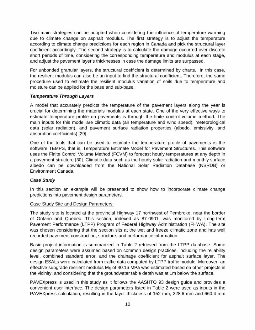
defined according to Table 3.

Material Type Identifier Color Specific Heat Capacity (J/kg*K)

Conductivity (W/m*K)

Density (kg/m3)

AC Black 1298 1.9 2374

Base Gray 1038 3.73 2330

Sub-base Gray 1131 4.065 2446

Subgrade Gray 710 1.6 1550

Table 3: Material Property Definition at TEMPS

The next step was to define the climatic data, which includes hourly air temperature, wind speed

and solar radiation, according to the downloaded materials from the National Solar Radiation

Database (NSRDB). The hourly albedo values were also taken from the NSRDB Database and

the monthly average was calculated to input in TEMPS.

This is followed by the definition of the pavement structure, that is, the thickness of the layers,

and lastly by the generation of the pavement mesh. The mesh will determine how many points

13

the software will calculate for the temperature along the pavement depth. For this example, the

mesh was chosen as 1 cm.

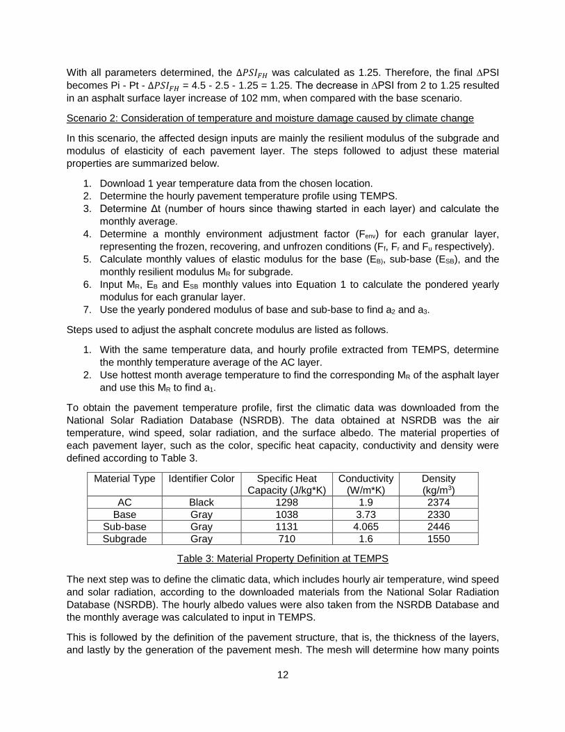
To estimate the resilient modulus of the materials under different circumstances, three main

parameters are crucial, the percent passing No. 200 sieve, 𝑃200, the effective grain size

corresponding to 60% passing by weight, 𝐷60, and the plasticity index (PI). Table 4 presents

those three inputs considered for each unbonded layer. Note that these properties are the same

as used in the base scenario.

Table 4: Gradation and Properties of the Unbound Materials

Layer 𝑃200 (%) 𝐷60 (%) PI

Base 5 13.3 5

Sub-base 7.5 2 6

Subgrade 70 0.01 12

Referring to Equation 2, the parameters 𝑎, 𝑏, and 𝑘𝑚 varies for coarse-grained and fine-grained

materials. Therefore, according to the MEPDG table 2.3.8, the base and sub-base 𝑎, 𝑏, and 𝑘𝑚

were defined as -0.3123, 0.3 and 6.8157, respectively, while the subgrade 𝑎, 𝑏, and 𝑘𝑚 was -

0.5934, 0.4 and 0.1324. The drop in the resilient modulus due to the thawing of the pavement

layers can be estimated through a reduction factor RF, as expressed in Equation 3 [27].

𝑅𝐹 =𝑀𝑅𝑚𝑖𝑛

𝑠𝑚𝑎𝑙𝑙𝑒𝑟 𝑜𝑓 (𝑀𝑅𝑓𝑢𝑛𝑟𝑧, 𝑀𝑅𝑜𝑝𝑡) Equation 3

Where, 𝑀𝑅𝑓𝑢𝑛𝑟𝑧 is the natural unfrozen resilient modulus and 𝑀𝑅𝑚𝑖𝑛 is the thawed resilient

modulus, which corresponds to the weakest resilient modulus the material will present during

the year. The subgrade frozen resilient modulus for this example was determined in the field

and it is equal to 138 MPa [31].

The reduction of the soil stiffness with thawing is directly related to frost susceptibility, so the

recommended reduction factor RF of the subgrade is dependent on the percent passing No.

200 sieve, 𝑃200, and the plasticity index (PI). In the case study, the recommended factor is 0.55,

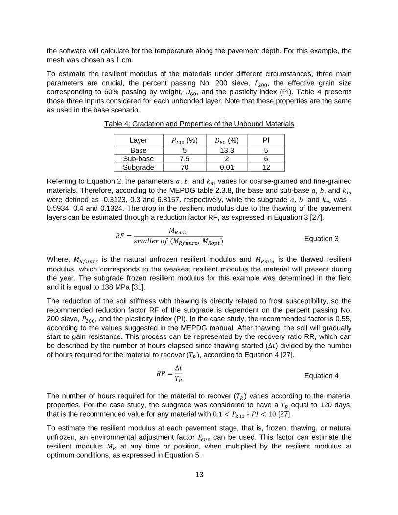
according to the values suggested in the MEPDG manual. After thawing, the soil will gradually

start to gain resistance. This process can be represented by the recovery ratio RR, which can

be described by the number of hours elapsed since thawing started (∆𝑡) divided by the number

of hours required for the material to recover (𝑇𝑅), according to Equation 4 [27].

𝑅𝑅 =∆𝑡

𝑇𝑅 Equation 4

The number of hours required for the material to recover (𝑇𝑅) varies according to the material

properties. For the case study, the subgrade was considered to have a 𝑇𝑅 equal to 120 days,

that is the recommended value for any material with 0.1 < 𝑃200 ∗ 𝑃𝐼 < 10 [27].

To estimate the resilient modulus at each pavement stage, that is, frozen, thawing, or natural

unfrozen, an environmental adjustment factor 𝐹𝑒𝑛𝑣 can be used. This factor can estimate the

resilient modulus 𝑀𝑅 at any time or position, when multiplied by the resilient modulus at

optimum conditions, as expressed in Equation 5.

14

𝑀𝑅 = 𝐹𝑒𝑛𝑣 ∗ 𝑀𝑅𝑜𝑝𝑡 Equation 5

Where, 𝐹𝑒𝑛𝑣 is the adjustment factor, and 𝑀𝑅𝑜𝑝𝑡 is the resilient modulus at optimum conditions.

The number of hours elapsed since thawing started (∆𝑡) is the key to define 𝐹𝑒𝑛𝑣. If ∆𝑡 is equal

to 0, the soil is frozen, therefore 𝐹𝑒𝑛𝑣 is equal to 𝐹𝑓, if ∆𝑡 is between 0 and 2880 hours (120

days), then 𝐹𝑒𝑛𝑣 is equal to 𝐹𝑟, which means that the soil is under the recovery period, and if ∆𝑡

is greater than 2880 hours, it means that the soil has already recovered and is unfrozen,

therefore, 𝐹𝑒𝑛𝑣 is equal to 𝐹𝑢. The steps to compute 𝐹𝑓, 𝐹𝑟 and 𝐹𝑢 are described in the MEPDG

manual.

Scenario 2 is further broken into 3 sub-scenarios, as described below:

Scenario 2.1 assumes the temperatures remain unchanged throughout the 20-years

performance period and the ground water table is at 0.5 m below subgrade surface.

Scenario 2.2 considers a temperature increase of 15.08% and the ground water table at

1 m below subgrade surface.

Scenario 2.3 considers a temperature increase of 15.08% and the ground water table at

0.5 m below subgrade surface.

The temperature increase of 15.08% is chosen from temperature projection at the study site, in

which the data was downloaded from ClimateData.ca, for a performance period of 20 years

starting in 2020, under RCP 4.5. Following the steps mentioned previously, the subgrade

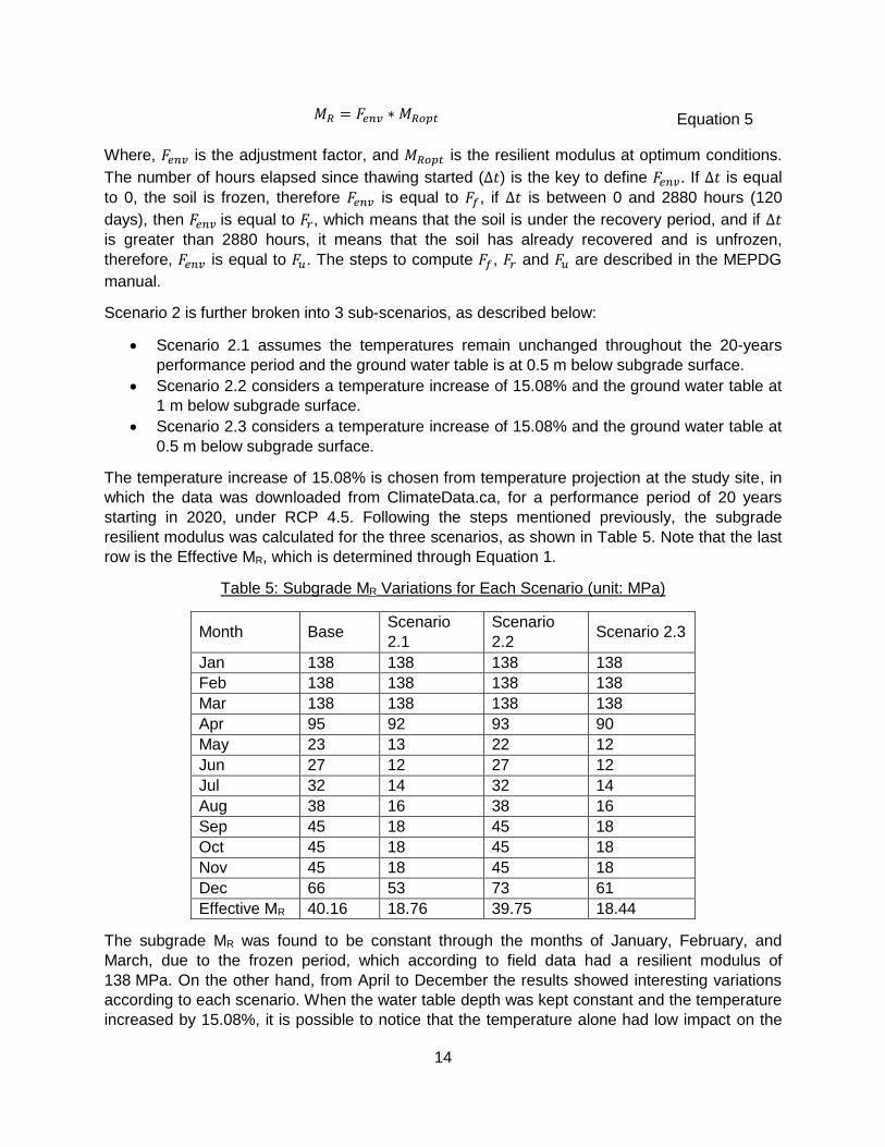
resilient modulus was calculated for the three scenarios, as shown in Table 5. Note that the last

row is the Effective MR, which is determined through Equation 1.

Table 5: Subgrade MR Variations for Each Scenario (unit: MPa)

Month Base Scenario

2.1

Scenario

2.2 Scenario 2.3

Jan 138 138 138 138

Feb 138 138 138 138

Mar 138 138 138 138

Apr 95 92 93 90

May 23 13 22 12

Jun 27 12 27 12

Jul 32 14 32 14

Aug 38 16 38 16

Sep 45 18 45 18

Oct 45 18 45 18

Nov 45 18 45 18

Dec 66 53 73 61

Effective MR 40.16 18.76 39.75 18.44

The subgrade MR was found to be constant through the months of January, February, and

March, due to the frozen period, which according to field data had a resilient modulus of

138 MPa. On the other hand, from April to December the results showed interesting variations

according to each scenario. When the water table depth was kept constant and the temperature

increased by 15.08%, it is possible to notice that the temperature alone had low impact on the

15

resilient modulus of the subgrade. That became evident, since when comparing the base

scenario and 2.2, there is an effective resilient modulus decrease of only 1.02%, while in

scenarios 2.1 and 2.3 the decrease was 1.7%. The impact of moisture variation, however, is

much higher. In the simulations, if the water table depth goes from 1 m to 0.5 m below the

subgrade surface, the effective resilient modulus of the subgrade can become 53.3% lower,

comparing the base scenario and 2.1, and 53.6% lower, comparing scenarios 2.2 and 2.3.

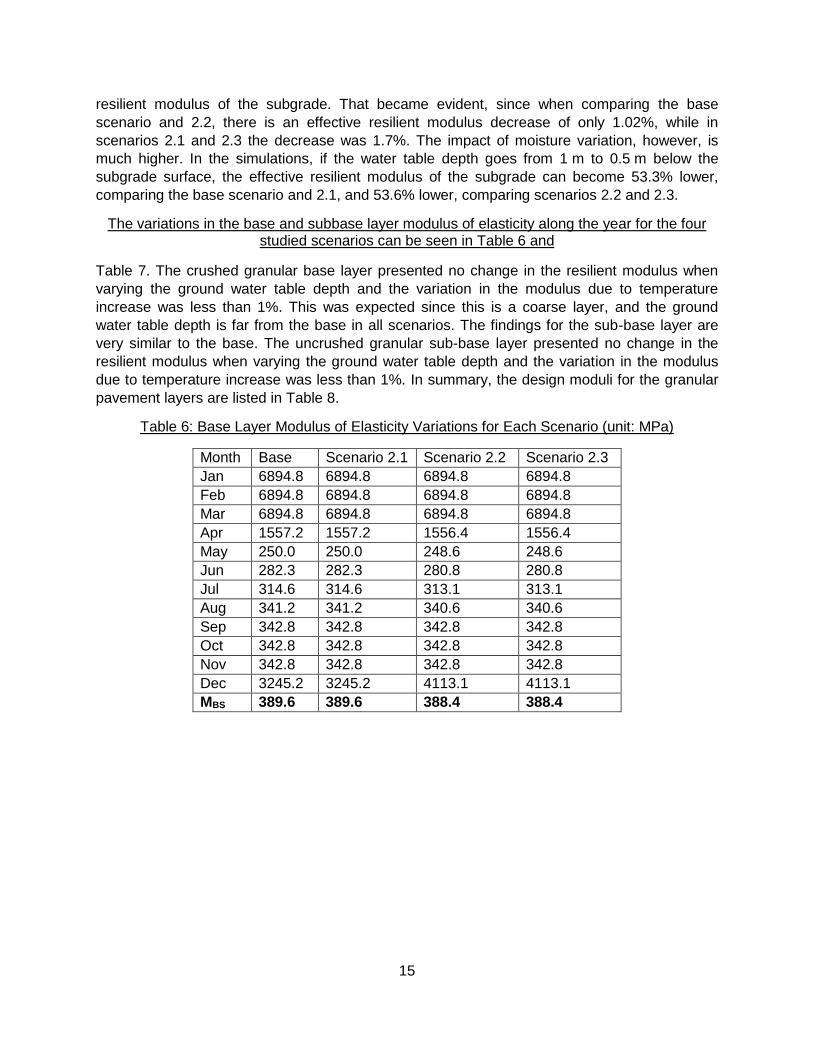
The variations in the base and subbase layer modulus of elasticity along the year for the four studied scenarios can be seen in Table 6 and

Table 7. The crushed granular base layer presented no change in the resilient modulus when

varying the ground water table depth and the variation in the modulus due to temperature

increase was less than 1%. This was expected since this is a coarse layer, and the ground

water table depth is far from the base in all scenarios. The findings for the sub-base layer are

very similar to the base. The uncrushed granular sub-base layer presented no change in the

resilient modulus when varying the ground water table depth and the variation in the modulus

due to temperature increase was less than 1%. In summary, the design moduli for the granular

pavement layers are listed in Table 8.

Table 6: Base Layer Modulus of Elasticity Variations for Each Scenario (unit: MPa)

Month Base Scenario 2.1 Scenario 2.2 Scenario 2.3

Jan 6894.8 6894.8 6894.8 6894.8

Feb 6894.8 6894.8 6894.8 6894.8

Mar 6894.8 6894.8 6894.8 6894.8

Apr 1557.2 1557.2 1556.4 1556.4

May 250.0 250.0 248.6 248.6

Jun 282.3 282.3 280.8 280.8

Jul 314.6 314.6 313.1 313.1

Aug 341.2 341.2 340.6 340.6

Sep 342.8 342.8 342.8 342.8

Oct 342.8 342.8 342.8 342.8

Nov 342.8 342.8 342.8 342.8

Dec 3245.2 3245.2 4113.1 4113.1

MBS 389.6 389.6 388.4 388.4

16

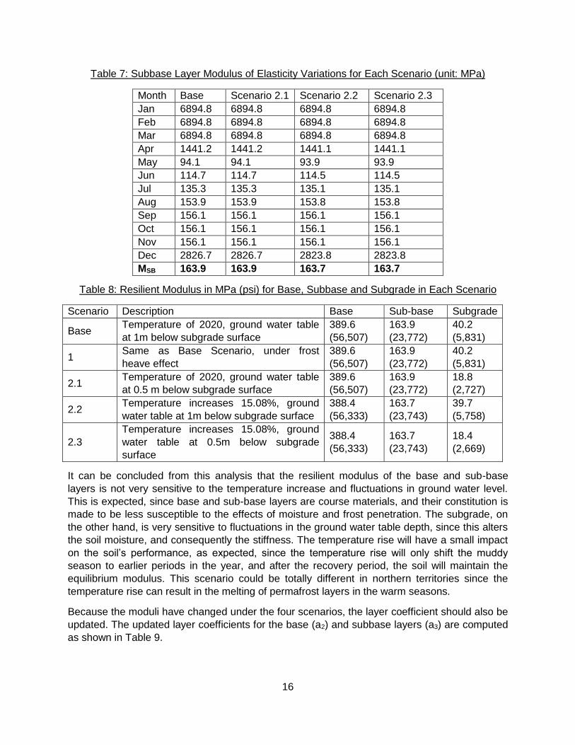
Table 7: Subbase Layer Modulus of Elasticity Variations for Each Scenario (unit: MPa)

Month Base Scenario 2.1 Scenario 2.2 Scenario 2.3

Jan 6894.8 6894.8 6894.8 6894.8

Feb 6894.8 6894.8 6894.8 6894.8

Mar 6894.8 6894.8 6894.8 6894.8

Apr 1441.2 1441.2 1441.1 1441.1

May 94.1 94.1 93.9 93.9

Jun 114.7 114.7 114.5 114.5

Jul 135.3 135.3 135.1 135.1

Aug 153.9 153.9 153.8 153.8

Sep 156.1 156.1 156.1 156.1

Oct 156.1 156.1 156.1 156.1

Nov 156.1 156.1 156.1 156.1

Dec 2826.7 2826.7 2823.8 2823.8

MSB 163.9 163.9 163.7 163.7

Table 8: Resilient Modulus in MPa (psi) for Base, Subbase and Subgrade in Each Scenario

Scenario Description Base Sub-base Subgrade

Base Temperature of 2020, ground water table

at 1m below subgrade surface

389.6

(56,507)

163.9

(23,772)

40.2

(5,831)

1 Same as Base Scenario, under frost

heave effect

389.6

(56,507)

163.9

(23,772)

40.2

(5,831)

2.1 Temperature of 2020, ground water table

at 0.5 m below subgrade surface

389.6

(56,507)

163.9

(23,772)

18.8

(2,727)

2.2 Temperature increases 15.08%, ground

water table at 1m below subgrade surface

388.4

(56,333)

163.7

(23,743)

39.7

(5,758)

2.3

Temperature increases 15.08%, ground

water table at 0.5m below subgrade

surface

388.4

(56,333)

163.7

(23,743)

18.4

(2,669)

It can be concluded from this analysis that the resilient modulus of the base and sub-base

layers is not very sensitive to the temperature increase and fluctuations in ground water level.

This is expected, since base and sub-base layers are course materials, and their constitution is

made to be less susceptible to the effects of moisture and frost penetration. The subgrade, on

the other hand, is very sensitive to fluctuations in the ground water table depth, since this alters

the soil moisture, and consequently the stiffness. The temperature rise will have a small impact

on the soil’s performance, as expected, since the temperature rise will only shift the muddy

season to earlier periods in the year, and after the recovery period, the soil will maintain the

equilibrium modulus. This scenario could be totally different in northern territories since the

temperature rise can result in the melting of permafrost layers in the warm seasons.

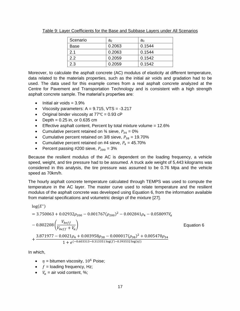
Because the moduli have changed under the four scenarios, the layer coefficient should also be

updated. The updated layer coefficients for the base (a2) and subbase layers (a3) are computed

as shown in Table 9.

17

Table 9: Layer Coefficients for the Base and Subbase Layers under All Scenarios

Scenario a2 a3

Base 0.2063 0.1544

2.1 0.2063 0.1544

2.2 0.2059 0.1542

2.3 0.2059 0.1542

Moreover, to calculate the asphalt concrete (AC) modulus of elasticity at different temperature,

data related to the materials properties, such as the initial air voids and gradation had to be

used. The data used for this example comes from a real asphalt concrete analyzed at the

Centre for Pavement and Transportation Technology and is consistent with a high strength

asphalt concrete sample. The material’s properties are:

Initial air voids = 3.9%

Viscosity parameters: A = 9.715, VTS = -3.217

Original binder viscosity at 77℃ = 0.93 cP

Depth = 0.25 in, or 0.635 cm

Effective asphalt content, Percent by total mixture volume = 12.6%

Cumulative percent retained on ¾ sieve, 𝑃34 = 0%

Cumulative percent retained on 3/8 sieve, 𝑃38 = 19.70%

Cumulative percent retained on #4 sieve, 𝑃4 = 45.70%

Percent passing #200 sieve, 𝑃200 = 3%

Because the resilient modulus of the AC is dependent on the loading frequency, a vehicle

speed, weight, and tire pressure had to be assumed. A truck axle weight of 5,443 kilograms was

considered in this analysis, the tire pressure was assumed to be 0.76 Mpa and the vehicle

speed as 70km/h.

The hourly asphalt concrete temperature calculated through TEMPS was used to compute the

temperature in the AC layer. The master curve used to relate temperature and the resilient

modulus of the asphalt concrete was developed using Equation 6, from the information available

from material specifications and volumetric design of the mixture [27].

log(𝐸∗)

= 3.750063 + 0.02932𝜌200 − 0.001767(𝜌200)2 − 0.002841𝜌4 − 0.058097𝑉𝑎

− 0.802208 (𝑉𝑏𝑒𝑓𝑓

𝑉𝑏𝑒𝑓𝑓 + 𝑉𝑎)

+3.871977 − 0.0021𝜌4 + 0.003958𝜌38 − 0.000017(𝜌38)2 + 0.005470𝜌34

1 + 𝑒(−0.603313−0.313351 log(𝑓)−0.393532 log(𝜂))

Equation 6

In which,

𝜂 = bitumen viscosity, 106 Poise;

𝑓 = loading frequency, Hz;

𝑉𝑎 = air void content, %;

18

𝑉𝑏𝑒𝑓𝑓 = effective bitumen content, % by volume;

𝜌34 = cumulative % retained on the ¾ in sieve;

𝜌38 = cumulative % retained on the 3/8 in sieve;

𝜌4 = cumulative % retained on the No. 4 sieve;

𝜌200 = % passing the No. 200 sieve.

The bitumen viscosity under the studied temperature was calculated and imputed in the

dynamic modulus master curve. The equations used in this example to find the bitumen

viscosity can be found at the MEPDG Manual.

The average modulus of the hottest month of the year (July) was used to calculate the layer

coefficient for pavement structural design. The average modulus in the base scenario was

calculated as 2,136 MPa, while the average modulus for the 15.08% temperature increase was

1,843 MPa, a decrease of 14% in the AC stiffness.

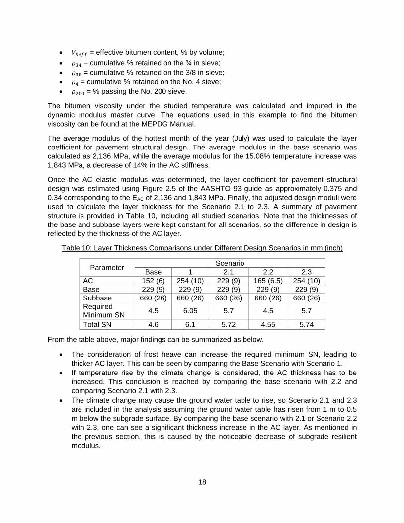
Once the AC elastic modulus was determined, the layer coefficient for pavement structural

design was estimated using Figure 2.5 of the AASHTO 93 guide as approximately 0.375 and

0.34 corresponding to the EAC of 2,136 and 1,843 MPa. Finally, the adjusted design moduli were

used to calculate the layer thickness for the Scenario 2.1 to 2.3. A summary of pavement

structure is provided in Table 10, including all studied scenarios. Note that the thicknesses of

the base and subbase layers were kept constant for all scenarios, so the difference in design is

reflected by the thickness of the AC layer.

Table 10: Layer Thickness Comparisons under Different Design Scenarios in mm (inch)

Parameter Scenario

Base 1 2.1 2.2 2.3

AC 152 (6) 254 (10) 229 (9) 165 (6.5) 254 (10)

Base 229 (9) 229 (9) 229 (9) 229 (9) 229 (9)

Subbase 660 (26) 660 (26) 660 (26) 660 (26) 660 (26)

Required Minimum SN

4.5 6.05 5.7 4.5 5.7

Total SN 4.6 6.1 5.72 4.55 5.74

From the table above, major findings can be summarized as below.

The consideration of frost heave can increase the required minimum SN, leading to

thicker AC layer. This can be seen by comparing the Base Scenario with Scenario 1.

If temperature rise by the climate change is considered, the AC thickness has to be

increased. This conclusion is reached by comparing the base scenario with 2.2 and

comparing Scenario 2.1 with 2.3.

The climate change may cause the ground water table to rise, so Scenario 2.1 and 2.3

are included in the analysis assuming the ground water table has risen from 1 m to 0.5

m below the subgrade surface. By comparing the base scenario with 2.1 or Scenario 2.2

with 2.3, one can see a significant thickness increase in the AC layer. As mentioned in

the previous section, this is caused by the noticeable decrease of subgrade resilient

modulus.

19

Conclusion

This research assessed the impacts of climate change in flexible pavements in Canada by

addressing climate projections and its consequences around the country. The study also

proposed a methodology for the incorporation of climatic projected changes in the design of

flexible pavements through AASHTO 93. An example was performed to illustrate the

incorporation of the climate change parameters, including temperature, precipitation/moisture,

and freeze-thaw cycles. The serviceability index, drainage coefficients, soil (subgrade) resilient

modulus, and layer coefficients were found to be the most sensitive pavement design

parameters. In the case study, the temperature increase was 15% in a design period of 20

years, but the proposed method for considering temperature rise can be applied for different

locations and any climate change projections. The results showed that temperature alone had a

low impact on the structural design, however, the climate change impacts were high when

associated with an increase in moisture levels. The impacts of temperature alone, however, can

be much higher in the areas affected by permafrost thawing.

References

[1] Environmnet and Climate Change Canada, "Canada’s Changing Climate Report," 2019.

[2] B. Mills, J. Andrey, J. Smith, S. Parm and K. Huen, "Road Well-Traveled: Implications of

Climate Change for Pavement Infrastructure in Southern Canada," Transportation

Association of Canada (TAC), 2007.

[3] S. L. Tighe, J. Smith, , B. Mills and J. Andrey, "Using the MEPDG to Assess Climate

Change Impacts on Southern Canadian Roads," in Seventh International Conference on

Managing Pavement Assets, 2008.

[4] J. T. Smith, S. L. Tighe, J. C. Andrey and B. Mil, "Temperature and Precipitation Sensitivity

Analysis on Pavement Performance - Report No. Weather 08-019," in Fourth National

Conference on Surface Transportation Weather; Seventh International Symposium on

Snow Removal and Ice Control Technology, 2008.

[5] American Association of State Highway and Transportation Officials, "AASHTO Guide for

Design of pavement structures," in Proceedings of the International Conference on

Sustainable Waste Management and Recycling: Construction Demolition Waste, 1993.

[6] Environment Canada, "A state of the environment report: The state of Canada’s climate:

monitoring variability and change (SOE Report No. 95-1. ISBN 0-662-23061-2. Cat. No.

En1-11/95-1E)," Government of Canada, 1995.

[7] S. Westra, L. V. Alexander and F. W. Zwiers, "Global increasing trends in annual maximum

daily precipitation," Journal of climate, vol. 26, no. 11, pp. 3904-3918, 2013.

[8] P. J. Williams, "Permafrost and climate change: geotechnical implications," Philosophical

Transactions of the Royal Society of London. Series A: Physical and Engineering Sciences,

vol. 352, no. 1699, pp. 347-358, 1995.

20

[9] H. Batenipour, "Understanding the performance of highway embankments on degraded

permafrost," University of Manitoba (Canada), 2012.

[10] I. M. Kettles, C. Tarnocai and S. D. Bauke, "Predicted permafrost distribution in Canada

under a climate warming scenario," Current Research, Geological Survey of Canada, 1997-

E, pp. 109-115, 1997.

[11] D. M. Lawrence and A. G. Slater, "A projection of severe near‐surface permafrost

degradation during the 21st century," Geophysical Research Letters, vol. 32, no. 24, 2005.

[12] Y. Zhang, W. Chen and D. W. Riseborough., "Disequilibrium response of permafrost thaw

to climate warming in Canada over 1850–2100," Geophysical Research Letters, vol. 35(2),

2008.

[13] J. S. Daniel and e. al, "Climate change: potential impacts on frost–thaw conditions and

seasonal load restriction timing for low-volume roadways," Road Materials and Pavement

Design, vol. 19, no. 5, pp. 1126-1146, 2018.

[14] American Association of State Highway and Transportation Officials, "Mechanistic-empirical

pavement design guide: a manual of practice," 2008.

[15] A. K. Apeagyei, J. R. Grenfell and G. D. Airey, "Influence of aggregate absorption and

diffusion properties on moisture damage in asphalt mixtures," Road Materials and

Pavement Design, vol. 16, no. sup1, pp. 404-422, 2015.

[16] P. S. Kandahl and I. J. Richards., "Premature failure of asphalt overlays from stripping:

Case histories," National Center for Asphalt Technology (US), 2001.

[17] A. Dawson, "Water in Road Structures," Dordrecht: Springer Netherlands, 2009.

[18] L. Korkiala-Tanttu, "Speed and reloading effects on pavement rutting," in Proceedings of

the Institution of Civil Engineers-Geotechnical Engineering, 2007.

[19] H. L. Theyse, "A mechanistic-empirical design model for unbound granular pavement

layers," University of Johannesburg, 2008.

[20] Z. Chen, S. E. Grasby and K. G. Osa, "Predicting average annual groundwater levels from

climatic variables: an empirical model," Journal of Hydrology, vol. 260, pp. 102-117, 2002.

[21] E. Simonsen and U. Isacsson, "Thaw weakening of pavement structures in cold regions,"

Cold regions science and technology, vol. 29, no. 2, pp. 135-151, 1999.

[22] K. O'Neill and R. D. Miller, "Exploration of a rigid ice model of frost heave," Water

Resources Research, vol. 21, no. 3, pp. 281-296, 1985.

[23] E. A. Abreu, "Impacts of Climate Change on Canadian Airport Pavements," University of

Waterloo, 2019.

[24] E. Özgan and S. Serin, "Investigation of certain engineering characteristics of asphalt

21

concrete exposed to freeze–thaw cycles," Cold Regions Science and Technology, vol. 85,

pp. 131-136, 2013.

[25] D. Feng and e. al., "Impact of salt and freeze–thaw cycles on performance of asphalt

mixtures in coastal frozen region of China," Cold Regions Science and Technology, vol. 62,

no. 1, pp. 34-41, 2010.

[26] W. Si and e. al., "Impact of freeze-thaw cycles on compressive characteristics of asphalt

mixture in cold regions," Journal of Wuhan University of Technology-Mater, vol. 30, no. 4,

pp. 703-709, 2015.

[27] Applied Reseach Associates Inc. ERES Division, "Guide for Mechanistic-Empirical Design

of New and Rehabilitated Pavement StructuresAppendix DD-1: Resilient Modulus as

Function of Soil Moisture-Summary of Predictive Models - Final Document," Champaign, IL,

2000.

[28] H. Simpson, "Ground Water - An Important Rural Resource, Understanding Groundwater,"

Queen’s Printer for Ontario - Ministry of Agriculture, Food and Rural Affairs, 2015.

[29] M. Z. Alavi, M. R. Pouranian and E. Y. Hajj, "Prediction of asphalt pavement temperature

profile with finite control volume method," Transportation Research Record, vol. 2456, no.

1, pp. 96-106, 2014.

[30] W. Liu and e. al, "Stormwater runoff and pollution retention performances of permeable

pavements and the effects of structural factors," Environmental Science and Pollution

Research, vol. 27, pp. 30831-30843, 2020.

[31] L. D’Amours and e. al., "Assessment of Subgrade Soils for Pavement Design for Highway

407, East Extension Pickering to Oshawa, Ontario," in TAC 2016: Efficient

Transportation‐Managing the Demand‐2016 Conference and Exhibition of the

Transportation Association of Canada, 2016.