Embed Size (px)
Citation preview
Natural Language Processing
SoSe 2017
Lexical Semantics
Dr. Mariana Neves May 29th, 2017

Word Meaning
● Considers the meaning(s) of a word in addition to its written form
● Word Sense: a discrete representation of an aspect of the meaning of a word
2

Lexeme
● An entry in a lexicon consisting of a pair: a form with a single meaning representation
● band (music group)● band (material)● band (wavelength)
3
(http://www.nict.go.jp/en/press/2011/12/26-01.html) (http://www.weiku.com/products/12426189/Polyester_Elastic_band_for_garment_underwear_shoe_bags.html) (http://clipart.me/band-material-with-the-enthusiasm-of-the-audience-silhouette-19222)
Lemma
● The grammatical form that is used to represent a lexeme
– Berlin
– band
4

Homonymy
● Words which have similar form but different meanings
– Homographs:
● Berlin (Germany's capital); Berlin (music band)● band (music group); band (material); band
(wavelength)
5
Homophones
● Words which have similar pronunciation but different writing and meaning
– write
– right
6

Semantics Relations
● Lexical relations among words (senses)
– Hyponymy (is-a relation) {parent: hypernym, child: hyponym}
● dog & animal
7
(http://animalia-life.com/dogs.html) (http://pic-zoom.com/pictures-animals.html)

Semantics Relations
● Lexical relations among words (senses)
– Meronymy (part-of relation)
● arm & body
8
(http://www.oxfordlearnersdictionaries.com/definition/american_english/arm_1)

Semantics Relations
● Lexical relations among words (senses)
– Synonymy
● fall & autumn
9
(http://pinitgallery.com/photo/f/fall-background/7/)

Semantics Relations
● Lexical relations among words (senses)
– Antonymy
● tall & short
10 (http://pixgood.com/tall-short.html)

WordNet
● A hierarchical database of lexical relations
● Three Separate sub-databases
– Nouns
– Verbs
– Adjectives and Adverbs
● Each word is annotated with a set of senses
● Available online or for download
– http://wordnetweb.princeton.edu/perl/webwn
11
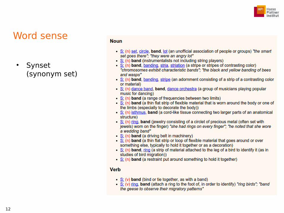
Word sense
● Synset (synonym set)
12

Word Relations (Hypernym)
13

Word sense disambiguation (WSD)
● Figure out the meaning of a word in a certain context
14

Motivation: Information retrieval & question answering
15

Motivation: Machine translation
16
(http://translate.google.de)

Motivation: Speech synthesis
● Eggs have a high protein content.
● She was content to step down after four years as chief executive.
17

Word Sense Disambiguation
● Input
– A word
– The context of the word
– Set of potential senses for the word
● Output
– The best sense of the word for this context
18
bank
The bank of the river was nice.
Ufer Bank

Approaches
● Thesaurus-based
● Supervised learning
● Semi-supervised learning
19
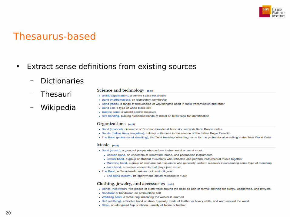
Thesaurus-based
● Extract sense definitions from existing sources
– Dictionaries
– Thesauri
– Wikipedia
20
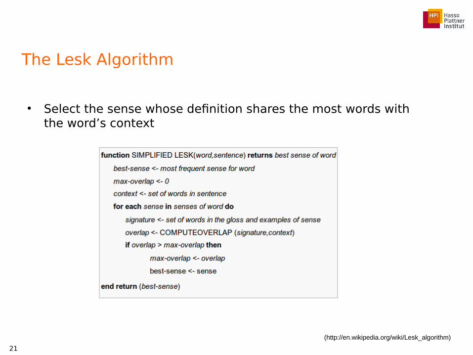
The Lesk Algorithm
● Select the sense whose definition shares the most words with the word’s context
21
(http://en.wikipedia.org/wiki/Lesk_algorithm)

The Lesk Algorithm
● Simple to implement
● No training data needed, „only“ a lexicon
● Relatively bad results
22

Supervised Learning
● Training data:
– A corpus in which each occurrence of the ambiguous word „w“ is annotated with its correct sense
● SemCor : 234,000 sense-tagged from Brown corpus● SENSEVAL-1: 34 target words● SENSEVAL-2: 73 target words● SENSEVAL-3: 57 target words (2081 sense-tagged)
23
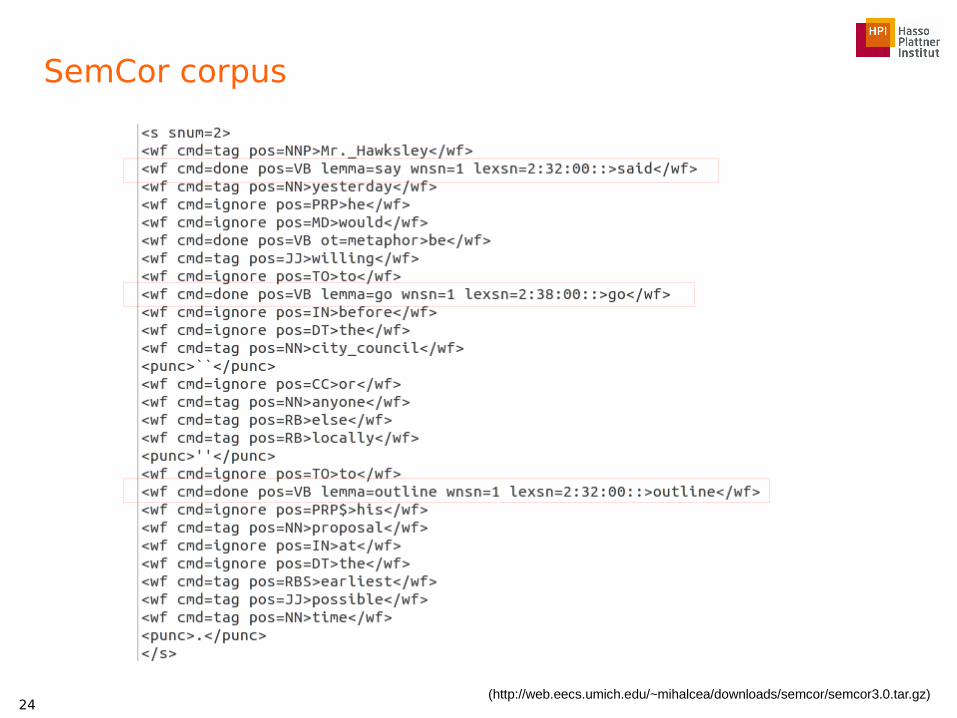
SemCor corpus
24(http://web.eecs.umich.edu/~mihalcea/downloads/semcor/semcor3.0.tar.gz)

Feature Selection
● Use the words in the context with a specific window size
– Collocation
● Consider all words in a window (as well as their POS) and their position:
25
{Wn−3,Pn−3,Wn−2,Pn−2 ,Wn−1,Pn−1,Wn+1,Pn+1 ,Wn+2 ,Pn+2 ,Wn+3,Pn+3}

Collocation: example
● band:
„There would be equal access to all currencies financial instruments and financial services dash and no major constitutional change. As realignments become more rare and exchange rates waver in narrower bands the system could evolve into one of fixed exchange rates.“
● Window size: +/- 3
● Context: waver in narrower bands the system could
● {Wn−3,Pn−3,Wn−2,Pn−2 ,Wn−1,Pn−1,Wn+1,Pn+1 ,Wn+2 ,Pn+2 ,Wn+3,Pn+3}
● {waver, NN, in , IN , narrower, JJ, the, DT, system, NN , could, MD}
26
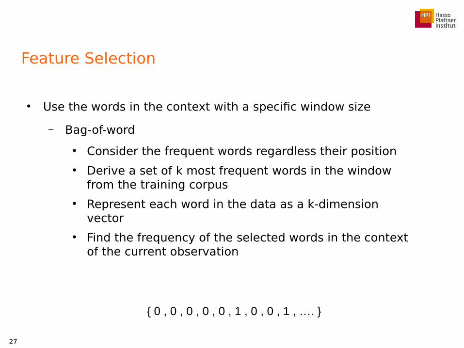
Feature Selection
● Use the words in the context with a specific window size
– Bag-of-word
● Consider the frequent words regardless their position● Derive a set of k most frequent words in the window
from the training corpus● Represent each word in the data as a k-dimension
vector● Find the frequency of the selected words in the context
of the current observation
27
{ 0 , 0 , 0 , 0 , 0 , 1 , 0 , 0 , 1 , …. }

Bag-of-words: example
● band:
„There would be equal access to all currencies financial instruments and financial services dash and no major constitutional change. As realignments become more rare and exchange rates waver in narrower bands the system could evolve into one of fixed exchange rates.“
● Window size: +/- 3
● Context: waver in narrower bands the system could
● k frequent words for „band“:
– {circle, dance, group, jewelery, music, narrow, ring, rubber, wave}
– { 0 , 0 , 0 , 0 , 0 , 1 , 0 , 0 , 1 }
28

Naïve Bayes Classification
● Choose the best sense ŝ out of all possible senses si for a feature vector f of the word w
29
s=argmax siP (s i∣ f )
s=argmax si
P ( f ∣si)P (si)
P ( f )
P ( f )has noeffect
s=argmax siP ( f ∣s i)P ( si)
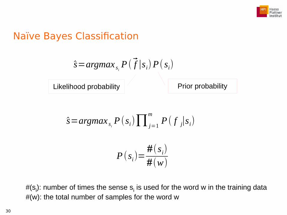
Naïve Bayes Classification
30
s=argmax siP ( f ∣si)P ( si)
Prior probabilityLikelihood probability
s=argmax siP (si)∏ j=1
mP ( f j∣si)
P (si)=#(si)
#(w)
#(si): number of times the sense si is used for the word w in the training data#(w): the total number of samples for the word w

Naïve Bayes Classification
31
s=argmax siP ( f ∣si)P ( si)
Prior probabilityLikelihood probability
s=argmax siP (si)∏ j=1
mP ( f j∣si)
#(fj,si): the number of times the feature fj occurred for the sense si of word w#(si): the total number of samples of w with the sense si in the training data
P ( f j∣si)=#( f j , si)
# si

Semi-supervised Learning
32
● A small amount of labeled data
● A large amount of unlabeled data
● Solution:
● Find the similarity between the labeled and unlabeled data
● Predict the labels of the unlabeled data
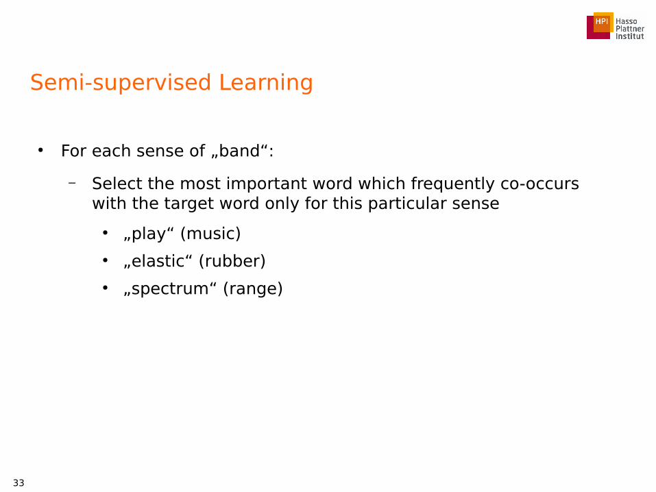
Semi-supervised Learning
● For each sense of „band“:
– Select the most important word which frequently co-occurs with the target word only for this particular sense
● „play“ (music)● „elastic“ (rubber)● „spectrum“ (range)
33

Semi-supervised Learning
● For each sense of „band“:
– Find the sentences from unlabeled data which contain the target word and the selected word
34
For example the Jamaican reggae musician Bob Marley and his band The Wailers were known to play the concerts ….
A rubber band, also known as a binder, elastic band, lackey band, laggy band, "gum band", or elastic, is a short length of rubber and latex, elastic in nature and formed ...
The band spectrum is the combination of many different spectral lines
(http://en.wikipedia.org/wiki/Encore_(concert)) (http://en.wikipedia.org/wiki/Rubber_band) (http://en.wikipedia.org/wiki/Spectral_bands)

Semi-supervised Learning
● For each sense,
– Label the sentence with the corresponding sense
– Add the new labeled sentences to the training data
35

Word similarity
● Task
– Find the similarity between two words in a wide range of relations (e.g., relatedness)
– Different of synonymy
– Being defined with a score (degree of similarity)
36

Word similarity
37
bank fund0.8
car bicycle0.5
car gasoline0.2
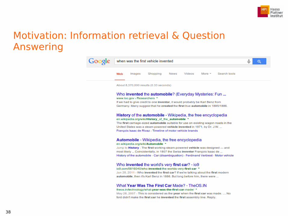
Motivation: Information retrieval & Question Answering
38

Motivation: Document categorization
39

Motivation: Machine translation, summarization, text generation
● Substitute of one word for other in some contexts
– „The bank is on the left bank of the river“
● „The financial institution is on the left bank of the river“
40

Motivation: Word clustering
41 (http://neoformix.com/2009/WorldNewsClusteredWordCloud.html)

Approaches
● Thesaurus-based
– Based on their distance in a thesaurus
– Based on their definition in a thesaurus (gloss)
● Distributional
– Based on the similarity between their contexts
42

Thesaurus-based Methods
● Two concepts (sense) are similar if they are “nearby” (short path in the hypernym hierarchy)
43
nickel dime
coin
coinage
currency
medium of exchange
standard
scale
Richter scalemoney
fund
budget
12
57

Path-base Similarity
● pathlen(c1,c2) = 1 + number of edges in the shortest path between the sense nodes c1 and c2
● simpath(c1,c2) = − log pathlen(c1,c2)
● wordsim(w1,w2) = max c1∈senses(w1), c2 ∈senses(w2) sim(c1,c2)
when we have no knowledge about the exact sense
(which is the case when processing general text)
44

Path-base Similarity
● Shortcoming
– Assumes that each link represents a uniform distance
● „nickel“ to „money“ seems closer than „nickel“ to „standard“
45
nickel dime
coin
coinage
currency
medium of exchange
standard
scale
Richter scalemoney
fund
budget
5
5

Path-base Similarity
● Use a metric which represents the cost of each edge independently
⇒ Words connected only through abstract nodes are less similar
46
nickel dime
coin
coinage
currency
medium of exchange
standard
scale
Richter scalemoney
fund
budget
5
4.5

Information Content Similarity
● Assign a probability P(c) to each node of thesaurus
– P(c) is the probability that a randomly selected word in a corpus is an instance of concept c
⇒ P(root) = 1, since all words are subsumed by the root concept
– The probability is trained by counting the words in a corpus
– The lower a concept in the hierarchy, the lower its probability
47
P(c)=∑w∈words(c)
#w
N
- words(c) is the set of words subsumed by concept c- N is the total number of words in the corpus that are available in thesaurus

Information Content Similarity
48
nickel dime
coin
coinage
currency
medium of exchange
standard
scale
Richter scalemoney
fund
budget
words(coin) = {nickel, dime}words(coinage) = {nickel, dime, coin}words(money) = {budget, fund}words(medium of exchange) = {nickel, dime, coin, coinage, currency, budget, fund, money}
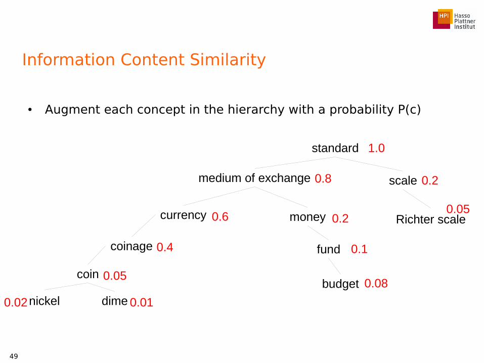
Information Content Similarity
● Augment each concept in the hierarchy with a probability P(c)
49
nickel dime
coin
coinage
currency
medium of exchange
standard
scale
Richter scalemoney
fund
budget
1.0
0.8 0.2
0.050.6 0.2
0.1
0.08
0.4
0.010.02
0.05

Information Content Similarity
● Information Content (self-information):
IC(c) = − log P(c)
50
nickel dime
coin
coinage
currency
medium of exchange
standard
scale
Richter scalemoney
fund
budget
1.0
0.8 0.2
0.050.6 0.2
0.1
0.08
0.4
0.010.02
0.05
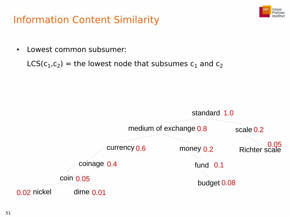
Information Content Similarity
● Lowest common subsumer:
LCS(c1,c2) = the lowest node that subsumes c1 and c2
51
nickel dime
coin
coinage
currency
medium of exchange
standard
scale
Richter scalemoney
fund
budget
1.0
0.8 0.2
0.050.6 0.2
0.1
0.08
0.4
0.010.02
0.05

Information Content Similarity
● Resnik similarity
– Measure the common amount of information by the information content of the lowest common subsumer of the two concepts
52
simresnik(c1,c2) = − log P(LCS(c1,c2))
simresnik(dime,nickel) = − log P(coin)
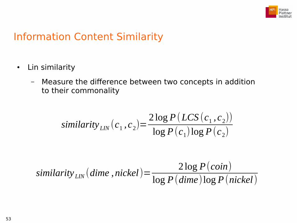
Information Content Similarity
● Lin similarity
– Measure the difference between two concepts in addition to their commonality
53
similarityLIN (c1 , c2)=2 log P (LCS (c1 , c2))
log P (c1) log P (c2)
similarity LIN (dime ,nickel )=2 log P (coin)
log P (dime) log P (nickel )

Information Content Similarity
● Jiang-Conrath similarity
54
similarity JC (c1 , c2)=1
log P (c1)+log P (c2)−2 log P (LCS (c1 , c2))

Extended Lesk
● Look at word definitions in thesaurus (gloss)
● Measure the similarity based on the number of common words in their definition
● Add a score of n2 for each n-word phrase that occurs in both glosses
55
similarityeLesk= ∑r , q∈RELSoverlap (gloss (r (c1)) , gloss (q(c2)))
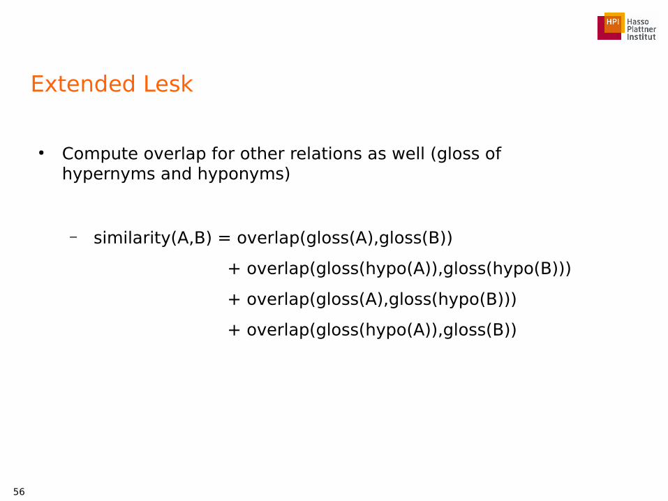
Extended Lesk
● Compute overlap for other relations as well (gloss of hypernyms and hyponyms)
– similarity(A,B) = overlap(gloss(A),gloss(B))
+ overlap(gloss(hypo(A)),gloss(hypo(B)))
+ overlap(gloss(A),gloss(hypo(B)))
+ overlap(gloss(hypo(A)),gloss(B))
56
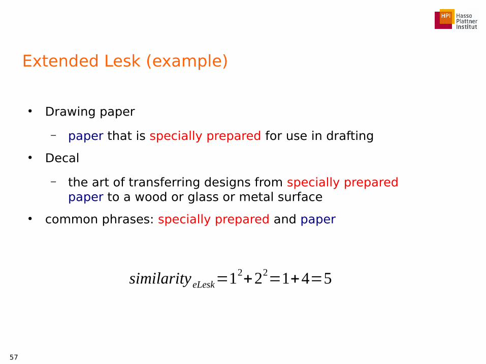
Extended Lesk (example)
● Drawing paper
– paper that is specially prepared for use in drafting
● Decal
– the art of transferring designs from specially prepared paper to a wood or glass or metal surface
● common phrases: specially prepared and paper
57
similarityeLesk=12+22=1+4=5

Available Libraries
● WordNet::Similarity
– Source:
● http://wn-similarity.sourceforge.net/
– Web-based interface:
● http://marimba.d.umn.edu/cgi-bin/similarity/similarity.cgi
21.05.201458

Thesaurus-based Methods
● Shortcomings
– Many words are missing in thesaurus
– Only use hyponym info
● Might useful for nouns, but weak for adjectives, adverbs, and verbs
– Many languages or domains have no thesaurus
● Alternative
– Distributional methods for word similarity
59

Distributional Methods
● Use context information to find the similarity between words
● Guess the meaning of a word based on its context
60
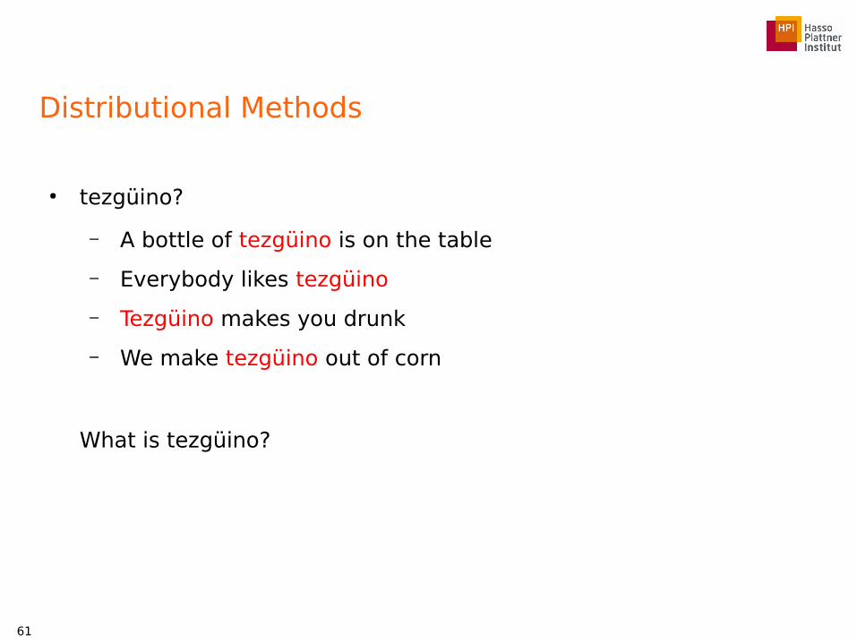
Distributional Methods
● tezgüino?
– A bottle of tezgüino is on the table
– Everybody likes tezgüino
– Tezgüino makes you drunk
– We make tezgüino out of corn
What is tezgüino?
61

Context Representations
● Consider a target term t
● Build a vocabulary of M words ({w1,w2,w3,...,wM})
● Create a vector for t with M features (t = {f1,f2,f3,...,fM})
● fi means the number of times the word wi occurs in the context of t
62

Context Representations
● tezgüino?
– A bottle of tezgüino is on the table
– Everybody likes tezgüino
– Tezgüino makes you drunk
– We make tezgüino out of corn
● t = tezgüino
vocab = {book, bottle, city, drunk, like, water,...}
t = { 0, 1 , 0 , 1 , 1 , 0 ,...}
63

Word vector or Word embeddings
● Frequently used in many neural networks architectures, e.g., morphology, language models
● Available tools: word2vec, GloVe
64
(https://www3.nd.edu/~dchiang/papers/vaswani-emnlp13.pdf)
(http://iiis.tsinghua.edu.cn/~weblt/papers/window-lstm-morph-segmentation.pdf)

Context Representations
● Term-term matrix
– The number of times the context word „c“ appear close to the term „t“ within a window
65
term / word art boil data function large sugar summarize water
apricot 0 1 0 0 1 2 0 1
pineapple 0 1 0 0 1 1 0 1
digital 0 0 1 3 1 0 1 0
information 0 0 9 1 1 0 2 0
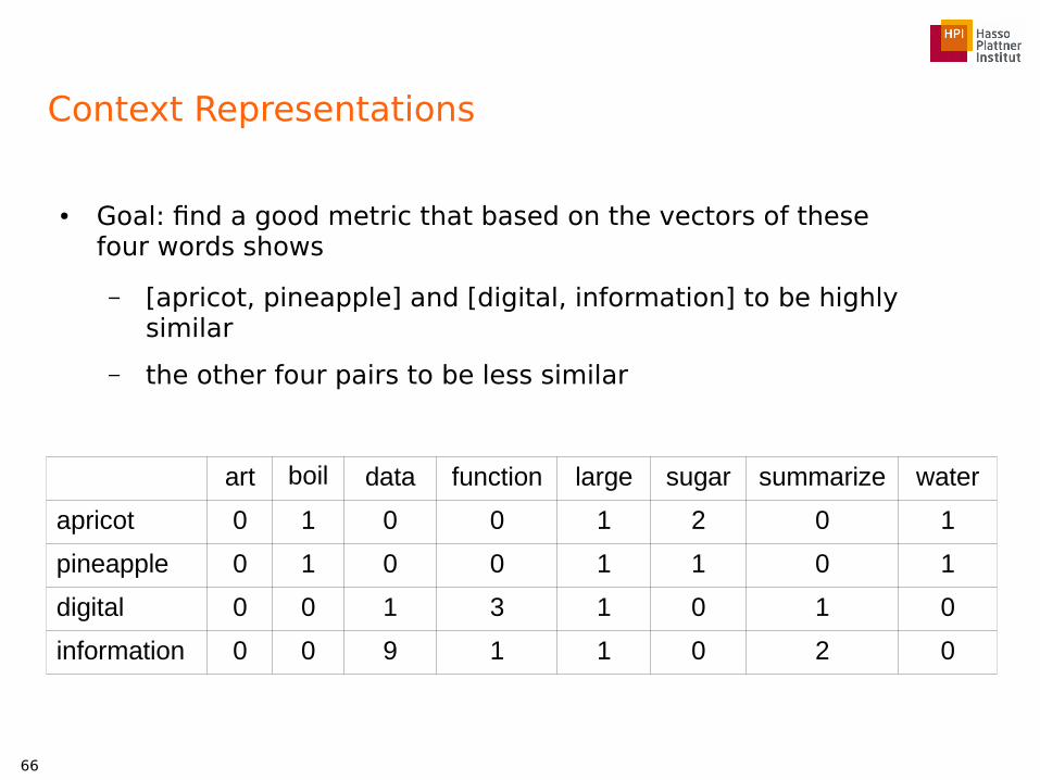
Context Representations
● Goal: find a good metric that based on the vectors of these four words shows
– [apricot, pineapple] and [digital, information] to be highly similar
– the other four pairs to be less similar
66
art boil data function large sugar summarize water
apricot 0 1 0 0 1 2 0 1
pineapple 0 1 0 0 1 1 0 1
digital 0 0 1 3 1 0 1 0
information 0 0 9 1 1 0 2 0

Distributional similarity
● Size of the context:
– How are the co-occurrence terms defined? (What is a neighbor?)
● Window of k words● Sentence● Paragraph● Document
67

Distributional similarity
● Weights: How are terms weighted?
– Binary
● 1, if two words co-occur (no matter how often)● 0, otherwise
68
term / word art boil data function large sugar summarize water
apricot 0 1 0 0 1 1 0 1
pineapple 0 1 0 0 1 1 0 1
digital 0 0 1 1 1 0 1 0
information 0 0 1 1 1 0 1 0

Distributional similarity
● Weights: How are terms weighted?
– Frequency
● Number of times two words co-occur with respect to the total size of the corpus
69
P (t , c)=#(t , c)
N

Distributional similarity
70
art boil data function large sugar summarize water
apricot 0 1 0 0 1 2 0 1
pineapple 0 1 0 0 1 1 0 1
digital 0 0 1 3 1 0 1 0
information 0 0 9 1 1 0 2 0
art boil data function large sugar summarize water
apricot 0 0.035 0 0 0.035 0.071 0 0.035
pineapple 0 0.035 0 0 0.035 0.035 0 0.035
digital 0 0 0.035 0.107 0.035 0 0.035 0
information 0 0 0.321 0.035 0.035 0 0.071 0
# (t,c)
P(t, c) {N = 28}

Distributional similarity
● Weights: How are terms weighted?
– Pointwise Mutual information
● Number of times two words co-occur, compared with what we would expect if they were independent
71
PMI (t , c)=logP (t , c)
P (t)P (c)

72
art boil data function large sugar summarize water
apricot 0 0.035 0 0 0.035 0.071 0 0.035
pineapple 0 0.035 0 0 0.035 0.035 0 0.035
digital 0 0 0.035 0.107 0.035 0 0.035 0
information 0 0 0.321 0.035 0.035 0 0.071 0
P(digital, summarize) = 0.035P(information, function) = 0.035
P(digital, summarize) = P(information, function)
PMI(digital, summarize) =?PMI(information, function) =?
Pointwise Mutual Information

Pointwise Mutual Information
73
art boil data function large sugar summarize water
apricot 0 0.035 0 0 0.035 0.071 0 0.035
pineapple 0 0.035 0 0 0.035 0.035 0 0.035
digital 0 0 0.035 0.107 0.035 0 0.035 0
information 0 0 0.321 0.035 0.035 0 0.071 0
P(digital, summarize) = 0.035P(information, function) = 0.035
P(digital) = 0.212 P(summarize) = 0.106P(function) = 0.142 P(information) = 0.462
PMI (digital , summarize )=P (digital , summarize )
P (digital ) · P ( summarize)=
0.0350.212 .0.106
=1.557
PMI (information , function)=P(information , function)
P (information) · P ( function)=
0.0350.462 .0.142
=0.533
PMI(digital, summarize) > PMI(information, function)

Distributional similarity
● Weights: How are terms weighted?
– t-test statistic
● How much more frequent the association is than by chance?
74
t−test (t , c)=P (t , c)−P (t)P (c)
√P (t )P (c)

Distributional similarity
● Vector similarity: Which vector distance metric should be used?
– Cosine
– Jaccard, Tanimoto, min/max
– Dice
75
similaritycosine( v , w)=∑i
v i×w i
√∑iv i
2√∑iw i
2
similarity jaccard ( v , w)=∑i
min(v i , w i)
∑imax (v i ,w i)
similaritydice(v , w)=2⋅∑i
min(v i ,w i)
∑i(v i+w i)

Summary
● Semantics
– Senses, relations
● Word disambiguation
– Thesaurus-based, (semi-) supervised learning
● Word similarity
– Thesaurus-based
– Distributional
● Features, weighting schemes and similarity algorithms
76

Further Reading
● Speech and Language Processing (3rd edition draft)
– https://web.stanford.edu/~jurafsky/slp3/
– Chapters 15 and 17
77


![SOSE Unit - We Are One[1]](https://img.pdfslide.us/doc/110x75/55275e7d550346d7358b47eb/sose-unit-we-are-one1.jpg)