Embed Size (px)
Citation preview
U. S. Department of Commerce
National Oceanic and Atmospheric Administration
National Weather Service
National Centers for Environmental Prediction
Office Note 414
Initial Results from Long-Term Measurements of Atmospheric
Humidity and Related Parameters in the Marine Boundary Layer
at Two Locations in the Gulf of Mexico'
Laurence C. Breaker 2, David B. Gilhousen 3 ,
Hendrik L. Tolman4 and Lawrence D. Burroughs 2
June 1996
THIS IS AN UNREVIEWED MANUSCRIPT, PRIMARILY INTENDED FOR INFORMAL
EXCHANGE OF INFORMATION AMONG THE NCEP STAFF MEMBERS
........................
1OPC Contribution Number 1242NOAAINational Weather Service, NCEP, Washington, D.C. 202333 NOANANational Weather Service, Data Buoy Center, Stennis
Space Center, MS 395294 UCAR Visiting Scientist
OPC CONTRIBUTIONS
No. 1. Burroughs, L. D., 1987: Development of Forecast Guidance for Santa Ana Conditions. National Weather Digest, Vol.12 No. 1,7pp.
No. 2. Richardson, W. S., D. J. Schwab, Y. Y. Chao, and D. M. Wright, 1986: Lake Erie Wave Height Forecasts Generated byEmpirical and Dynamical Methods -- Comparison and Verification. TechnicalNote, 23pp.
No. 3. Auer, S. J., 1986: Determination of Errors in LFM Forecasts Surface Lows Over the Northwest Atlantic Ocean.Technical Note/NMC Office Note No. 313, 17pp.
No. 4. Rao, D. B., S. D. Steenrod, and B. V. Sanchez, 1987: A Method of Calculating the Total Flow from A Given SeaSurface Topography. NASA Technical Memorandum 87799., l9pp.
No. 5. Feit, D. M., 1986: Compendium of Marine Meteorological and Oceanographic Products of the Ocean Products Center.NOAA Technical Memorandum NWS NMC 68, 93pp.
No. 6. Auer, S. J., 1986: A Comparison of the LFM, Spectral, and ECMWF Numerical Model Forecasts of DeepeningOceanic Cyclones During One Cool Season. Technical Note/NMC Office Note No. 312, 20pp.
No. 7. Burroughs, L. D., 1987: Development of Open Fog Forecasting Regions. Technical Note/NMC Office Note. No. 323.,36pp.
No. 8. Yu, T. W., 1987: A Technique of Deducing Wind Direction from Satellite Measurements of Wind Speed. MonthlyWeather Review, 115, 1929-1939.
No. 9. Auer, S. J., 1987: Five-Year Climatological Survey of the Gulf Stream System and Its Associated Rings. Journal ofGeophysical Research, 92, 11,709-11,726.
No. 10. Chao, Y. Y., 1987: Forecasting Wave Conditions Affected by Currents and Bottom Topography. Technical Note,1 pp.
No. 11. Esteva, D. C., 1987: The Editing and Averaging of Altimeter Wave and Wind Data. Technical Note, 4pp.
No. 12. Feit, D. M., 1987: Forecasting Superstructure Icing for Alaskan Waters. National Weather Digest, 12, 5-10.
No. 13. Sanchez, B. V., D. B. Rao, and S. D. Steenrod, 1987: Tidal Estimation in the Atlantic and Indian Oceans. MarineGeodesy, 10, 309-350.
No. 14. Gemmill, W. H., T. W. Yu, and D. M. Feit 1988: Performance of Techniques Used to Derive Ocean Surface Winds.Technical Note/NMC Office Note No. 330, 34pp.
No. 15. Gemmill, W. H., T. W. Yu, and D. M. Feit 1987: Performance Statistics of Techniques Used to Determine OceanSurface Winds. Conference Preprint, Workshop Proceedings AES/CMOS 2nd Workshop of Operational MeteorologyHalifax, Nova Scotia., 234-243.
No. 16. Yu, T. W., 1988: A Method for Determining Equivalent Depths of the Atmospheric Boundary Layer Over the Oceans.Journal of Geophysical Research. 93, 3655-3661.
No. 17. Yu, T. W., 1987: Analysis of the Atmospheric Mixed Layer Heights Over the Oceans. Conference Preprint, WorkshopProceedings AES/CMOS 2nd Workshop of Operational Meteorology, Halifax, Nova Scotia, 2, 425-432.
No. 18. Feit, D. M., 1987: An Operational Forecast System for Superstructure Icing. Proceedings Fourth ConferenceMeteorology and Oceanography of the Coastal Zone. 4pp.
No. 19. Esteva, D. C., 1988: Evaluation of Priliminary Experiments Assimilating Seasat Significant Wave Height into aSpectral Wave Model. Journal of Geophysical Research. 93, 14,099-14,105.
No. 20. Chao, Y. Y., 1988: Evaluation of Wave Forecast for the Gulf of Mexico. Proceedings Fourth Conference Meteorologyand Oceanography of the Coastal Zone, 42-49.
ABSTRACT
Measurements of boundary layer moisture have been acquired from Rotronic MP-100sensors deployed on two NDBC buoys in the northern Gulf of Mexico from June throughNovember 1993. For one sensor which was retrieved approximately 8 months afterdeployment, the post- and pre-calibrations agreed closely and fell well within WMOspecifications for accuracy. Buoy observations of relative humidity and supporting datawere used to calculate specific humidity, and the surface fluxes of latent and sensible heat.Specific humidities from the buoys were compared with observations of moisture obtainedfrom nearby ship reports and the correlations were generally high (0. 7 - 0.9). These datawere not sufficient, however, to confirm or refute a recent report of hysteresis that mayoccur with the Rotronic sensor.
The time series of specific humidity and the other buoy parameters revealed threeprimary scales of variability, small-scale (of the order of hours), synoptic-scale (severaldays), and seasonal (several months). The synoptic-scale variability was clearly dominant;it was event-like in character and occurred primarily during September, October, andNovember. Most of the synoptic-scale variability was due to frontal systems that droppeddown into the Gulf of Mexico from the continental U.S., followed by air masses which werecold and dry. Cross-correlation analyses of the buoy data indicated that both specifichumidity and air temperature served as tracers of the motion associated with propagatingatmospheric disturbances. Spectra of the various buoy parameters indicated strong diurnaland semidiurnal variability for barometric pressure and sea surface temperature (SST) andlesser variability for air temperature and wind speed.
The calculated surface fluxes of latent and sensible heat were dominated by thesynoptic events which took place from September through November. Mean Bowen ratioswere in the range 6 - 8%, indicating that the latent heat fluxes far exceeded the sensibleheat fluxes in this region. Finally, an analysis of the surface wave observations from eachbuoy, which included calculations of wave age and estimates of surface roughness, yieldedresults which are consistent with enhanced moisture exchange between the ocean and themarine boundary layer during periods of high latent heat flux.
1
1. INTRODUCTION
The acquisition of meteorological observations within the marine boundary layer hasalways posed unique problems due to the proximity of the ocean surface to the sensorlocation, and the constant state of motion of the surface itself. Atmospheric humidity hasbeen a particularly difficult parameter to measure near the ocean surface. First, it isdifficult to protect humidity sensors from salt spray which accumulates over time andconsequently degrades calibration accuracy; second, humidity sensors must beadequately protected excess heating due to incoming solar radiation; and finally, humiditysensors must recover from periods of saturation rapidly and without change to theircalibration (Coantic and Friehe 1980).
Since atmospheric moisture is a difficult parameter to measure accurately over theocean, it is not surprising that it has been even more difficult to acquire observations ofboundary layer moisture from unattended instruments for extended periods of severalmonths or more. Recently, however, a number of humidity sensors have been evaluatedfor possible use in measuring atmospheric moisture in the marine environment (e.g.,Semmer 1987; Muller and Beekman 1987; Crescenti et al. 1990; Katsaros et al. 1994).
Because of the continuing need for long-term measurements of moisture within themarine boundary layer, the National Data Buoy Center (NDBC) evaluated the Rotronic MP-100 humidity sensor for possible deployment on their moored ocean data buoys, basedon promising test results from Muller and Beekman (1987) and Semmer (1987). Initialfield tests were conducted along the U.S. West Coast in 1989. A Rotronic humidity sensorwas installed on a Coastal-Marine Automated Network (C-MAN) station at Point Arguello,California and showed high correlations between saturation events and restrictedvisibilities in fog. Calculated dew point temperatures following fog events were in generalagreement with those reported at Vandenberg Air Force Base located nearby. After a four-month evaluation, Rotronic humidity sensors were introduced on several NDBC buoys andC-MAN stations along the California coast, but, initially, several gross failures occurredwithin weeks after they were installed. A gross failure occurred when reported relativehumidities either:
* (1) exceeded 106%,* (2) remained at, or exceeded, 100% for a day or more after satellite imagery
indicated fog dissipation, or0* (3) disagreed by 30% or more with nearby reports for low values typically less then
30%.
These failures lead to several improvements to the Rotronic sensor and its installationaboard the NDBC buoy platforms.
2

* First, the cabling from the sensor to the on-board electronic payload was replaced.The original cables had inadequate insulation and cable flexing often producedlarge calibration shifts.
* Second, the method of calibration was changed by exposing the sensor to a seriesof different saturated salt solutions in closed flasks and then comparing theobserved relative humidities to the known equilibrium vapor pressure of water at theobserved temperatures for these solutions.
Test flasks with relative humidities ranging from 11 to 96% were used. Theseimprovements led to significantly greater measurement accuracy and sensor reliability.As a result, these instruments have been installed on a number of NDBC buoys since1989, concomitant with improvements in their performance.
As a basis for this study, we acquired hourly measurements of relative humidity andother supporting environmental data from two NDBC buoys in the Gulf of Mexico (Fig. 1)which were equipped with the improved Rotronic MP-100 humidity sensors for the period5 June to 30 November 1993. Initially, details of the sensor calibration, deployment andreliability are addressed. Then the relative humidity and supporting data from the buoysare used to calculate specific humidity and the corresponding fluxes of latent and sensibleheat. To provide a measure of validation for these observations, the moisture data arecompared with reports from nearby ships and other fixed platforms. A number of synopticevents occurred during the measurement period which provided an opportunity to examinethe response of the instrument to these events.
2. INSTRUMENT DESCRIPTION
a. Background
The Rotronic MP-100 humidity sensor has been under development since about 1980.Although the initial design was fragile and susceptible to contamination (Crane and Boole1988), recent versions of the instrument have proven more rugged and less sensitive tocontamination. The Rotronic MP-100 is classified as a thin film capacitive polymer sensor(Crescenti et al. 1990). The operation of the instrument's transducer is based on theprinciple of capacitance change as the polymer absorbs and desorbs water vapor. A Gor-Tex filter covers the transducer and allows water vapor (but not liquid water) to passthrough it. Contaminants reduce the passage of water vapor through the filter which canlead to erroneous reports of saturation following high moisture events. As a result, thefilter must be kept clean (Van der Meulen 1988). Although the Rotronic MP-100 sensorhas been used with relative success to measure moisture in the marine boundary layer,recent results in one case have indicated that this instrument may suffer from hysteresisafter periods of high relative humidity (Katsaros et al. 1994). This problem will bediscussed in greater detail in Sections 4a and 5 of this paper.
3
30°N
25°N
20°N
95°W 90°W 85°W
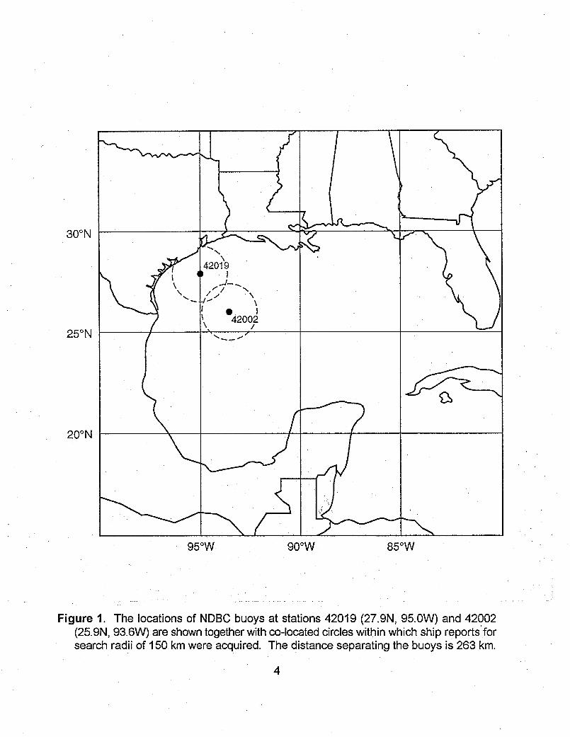
Figure 1. The locations of NDBC buoys at stations 42019 (27.9N, 95.0W) and 42002(25.9N, 93.6W) are shown together with co-located circles within which ship reports forsearch radii of 150 km were acquired. The distance separating the buoys is 263 km.
4

L.L
'~ -- i-';-
: ~~~~~~~~~
I~~ -~-.', ~"~. ,.-',- '--
~~~~ Jo t
Figure 2. The top panel (2a) shows a p42002. Note the small boat to thethe Rotronic sensor mounted on thismeters above the water line.
j�3�
� �
�'-� .- 4,
)hotograph of the 10 meter discus buoy moored atright for comparison. The lower panel (2b) showsbuoy. This instrument is located at a height of 10
5
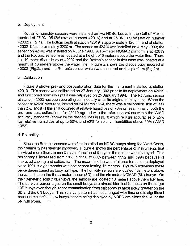
b. Deployment
Rotronic humidity sensors were installed on two NDBC buoys in the Gulf of Mexicolocated at 27.9N, 95.0W (station number 42019) and at 25.9N, 93.6W (station number42002) (Fig. 1). The bottom depth at station 42019 is approximately 120 m, and at station42002 it is approximately 3200 m. The sensor on 42019 was installed on 4 May 1993; thesensor on 42002 was installed on 4 June 1993. A six-meter NOMAD platform is at 42019and the Rotronic sensor was located at a height of 5 meters above the water line. Thereis a 10-meter discus buoy at 42002 and the Rotronic sensor in this case was located at aheight of 10 meters above the water line. Figure 2 shows the discus buoy moored at42002 (Fig.2a) and the Rotronic sensor which was mounted on this platform (Fig.2b).
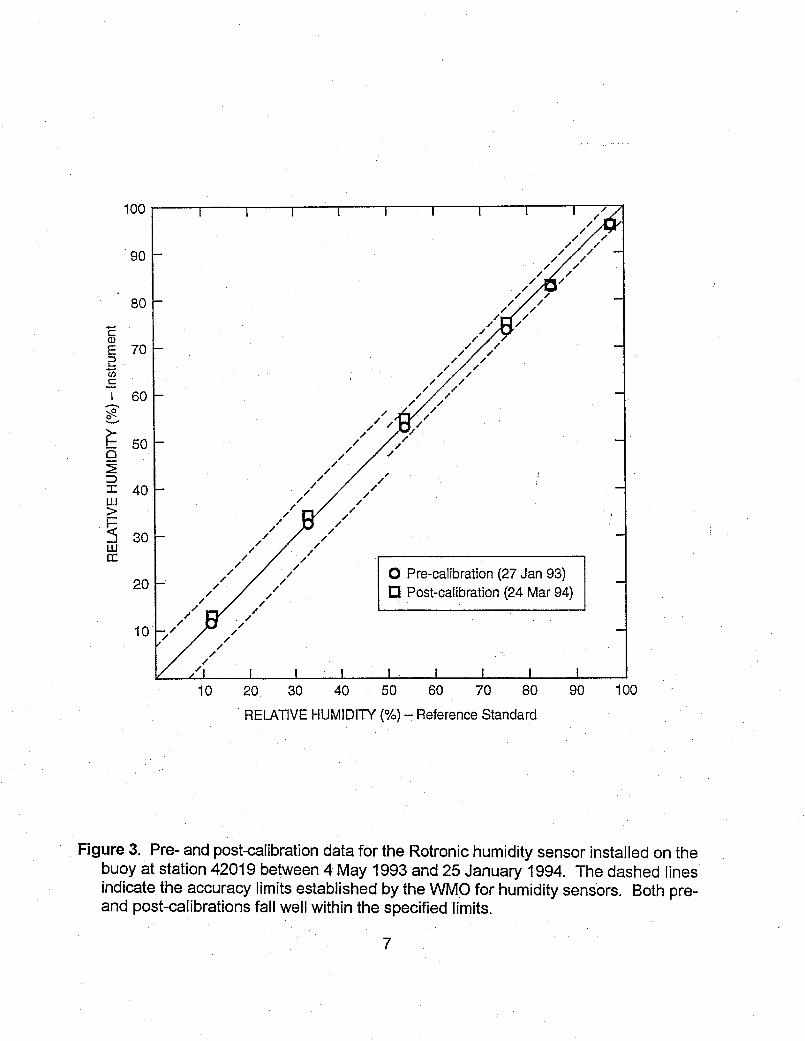
c. Calibration
Figure 3 shows pre- and post-calibration data for the instrument installed at station42019. This sensor was calibrated on 27 January 1993 prior to its deployment on 42019and functioned normally until it was retrieved on 25 January 1994. The Rotronic sensorat station 42002 has been operating continuously since its original deployment. When thesensor at 42019 was recalibrated on 24 March 1994, there was a calibration shift of lessthan 2%. Most of this shift occurred at relative humidities of 70% or less. Finally, both thepre- and post-calibrations for 42019 agreed with the reference values within the WMOaccuracy standards (shown by the dashed lines in Fig. 3) which require accuracies of +5%for relative humidities of up to 50%, and +2% for relative humidities above 50% (WMO1983).
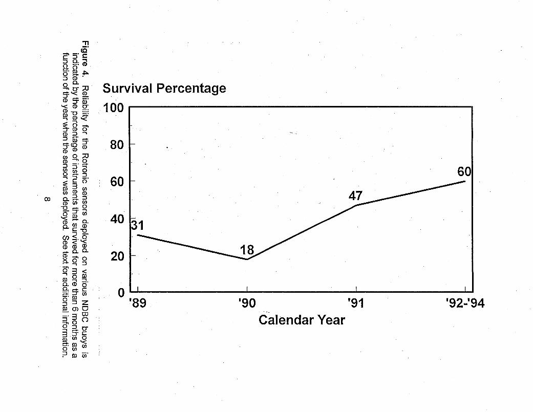
d. Reliability
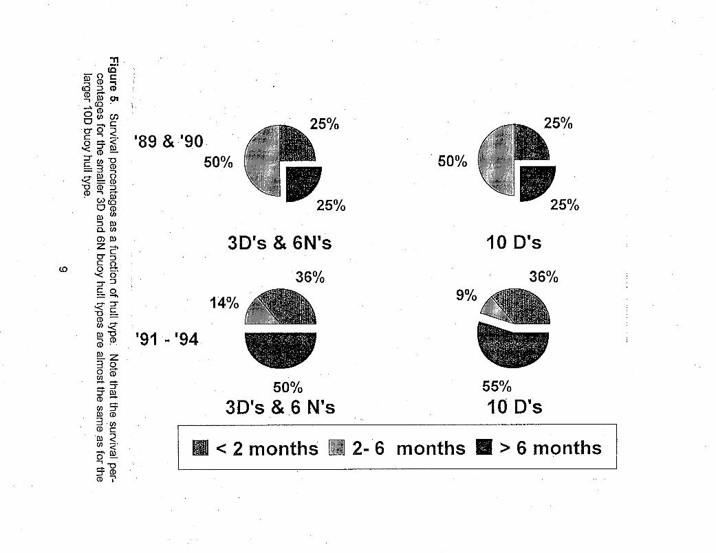
Since the Rotronic sensors were first installed on NDBC buoys along the West Coast,their reliability has steadily improved. Figure 4 shows the percentage of instruments thatsurvived more than six months as a function of the year the sensor was deployed. Thispercentage increased from 18% in 1990 to 60% between 1992 and 1994 because ofimproved cabling and calibration. The mean time between failures for sensors deployedsince 1991 is eight months with one sensor lasting 15 months. Figure 5 examines thesepercentages based on buoy hull type. The humidity sensors are located five meters abovethe water line on the three-meter discus (3D) and the six-meter NOMAD (6N) buoys. Onthe 10-meter discus (1 OD) buoys, the sensors are located 10 meters above the water line.The survival percentages on the small buoys are almost identical to those on the larger1 OD buoys even though senor contamination from salt spray is most likely greater on the3D and the 6N buoys. This survival pattern has not changed with time and is significantbecause most of the new buoys that are being deployed by NDBC are either the 3D or the6N hull types.
6
100
E
I
LU
Ci.E
.c
10 20 30 40 50 60 70 80
RELATIVE HUMIDITY (%) - Reference Standard
90 100
Figure 3. Pre- and post-calibration data for the Rotronic humidity sensor installed on thebuoy at station 42019 between 4 May 1993 and 25 January 1994. The dashed linesindicate the accuracy limits established by the WMO for humidity sensors. Both pre-and post-calibrations fall well within the specified limits.
7
-n
, -Q'3t
CD
(D (D
C t
'CD0
D.) C
(D 0
O tn lOo 1
C1
I (D -CD C:
:3' (D
Q Q
(0 D
(~ o :;0
CD tn
CDCDCD
(D_. O,
U) (D
°D
co CL ,~(D (a
a ~o
- 0.
(. D
.(: tn
CD - %.Q(DO( (
-0~
Co
PmD
Survival100
80
60
Percentage
60
r40
20
0 '89 '90 '91
Calendar Year
47
'92-'94
( 0 .
o '
'.~CD
C (D
'- -_ CD
(I D )
CDC
V3 w
o- (AO) i
:D '*
Cc
(D 0
Co~c
CD:
CD
_D
C_.Jn
.c-)
O --t.
0 (D
(DD
cn~-z
M CD
3oD
(D O :
*On
::r CD
CD O
:3'(-0) ?
25%39 & '90
50%
25%
25%
50%
25%
3D's & 6N's
36%9%14%
10 D's
36%
9) - '94
50%3D's & 6 N's
55%
10 D's
M < 2 months M 2-6 months M > 6 months
3. DATA ACQUISITION AND ANALYSIS
a. Acquisition
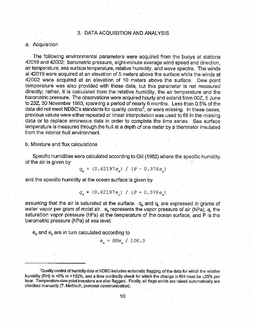
The following environmental parameters were acquired from the buoys at stations42019 and 42002: barometric pressure, eight-minute average wind speed and direction,air temperature, sea surface temperature, relative humidity, and wave spectra. The windsat 42019 were acquired at an elevation of 5 meters above the surface while the winds at42002 were acquired at an elevation of 10 meters above the surface. Dew pointtemperature was also provided with these data, but this parameter is not measureddirectly; rather, it is calculated from the relative humidity, the air temperature and thebarometric pressure. The observations were acquired hourly and extend from 00Z, 5 Juneto 23Z, 30 November 1993, spanning a period of nearly 6 months. Less than 0.5% of thedata did not meet NDBC's standards for quality control', or were missing. In these cases,previous values were either repeated or linear interpolation was used to fill in the missingdata or to replace erroneous data in order to complete the time series. Sea surfacetemperature is measured through the hull at a depth of one meter by a thermistor insulatedfrom the interior hull environment.
b. Moisture and flux calculations
Specific humidities were calculated according to Gill (1982) where the specific humidityof the air is given by
qa = (0.62197ea) / (P - 0.378ea)
and the specific humidity at the ocean surface is given by
q, = (0.62197es) / (P - 0.378es)
assuming that the air is saturated at the surface. qa and a, are expressed in grams ofwater vapor per gram of moist air. ea represents the vapor pressure of air (hPa), es thesaturation vapor pressure (hPa) at the temperature of the ocean surface, and P is thebarometric pressure (hPa) at sea level.
ea and es are in turn calculated according to
ea RHe / 100.0a $
'Quality control of humidity data at NDBC includes automatic flagging of the data for which the relativehumidity (RH) is <0% or >102%, and a time continuity check for which the change in RH must be <25% perhour. Temperature-dew point inversions are also flagged. Finally, all flags which are raised automatically arechecked manually (T. Mettlach, personal communication).
10
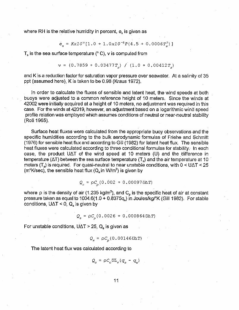
where RH is the relative humidity in percent, es is given as
e = KxlOv[1.O + 1.Ox10-6 P(4.5 + 0.0006Ts2 ) ]
Ts is the sea surface temperature (0 C), v is computed from
v = (0.7859 + 0.03477T) / (1.0 + 0.00412T)
and K is a reduction factor for saturation vapor pressure over seawater. At a salinity of 35ppt (assumed here), K is taken to be 0.98 (Kraus 1972).
In order to calculate the fluxes of sensible and latent heat, the wind speeds at bothbuoys were adjusted to a common reference height of 10 meters. Since the winds at42002 were initially acquired at a height of 10 meters, no adjustment was required in thiscase. For the winds at 42019, however, an adjustment based on a logarithmic wind speedprofile relation was employed which assumes conditions of neutral or near-neutral stability
(Roll 1965).
Surface heat fluxes were calculated from the appropriate buoy observations and thespecific humidities according to the bulk aerodynamic formulas of Friehe and Schmitt(1976) for sensible heat flux and according to Gill (1982) for latent heat flux. The sensibleheat fluxes were calculated according to three conditional formulas for stability.: In eachcase, the product UAT of the wind speed at 10 meters (U) and the difference intemperature (AT) between the sea surface temperature (Ts) and the air temperature at 10meters (Ta) is required. For quasi-neutral to near unstable conditions, with 0 < UAT < 25(m°K/sec), the sensible heat flux (Q, in W/m2) is given by
Qs = pC (0.00 2 + 0.00097UAT)
where p is the density of air (1.235 kg/m3), and Cp is the specific heat of air at constantpressure taken as equal to 1004.6(1.0 + 0.8375q%) in Joules/kg/?K (Gill 1982). For stableconditions, UAT < 0, Q5 is given by
Q = pC (0.0026 + 0.000864UAT).~~~~~~For unstable conditions, UAT > 25, Qs is given as
Q = pC (0.00146UAT)
The latent heat flux was calculated according to
Qe = pCeULv ( qs - q)
11
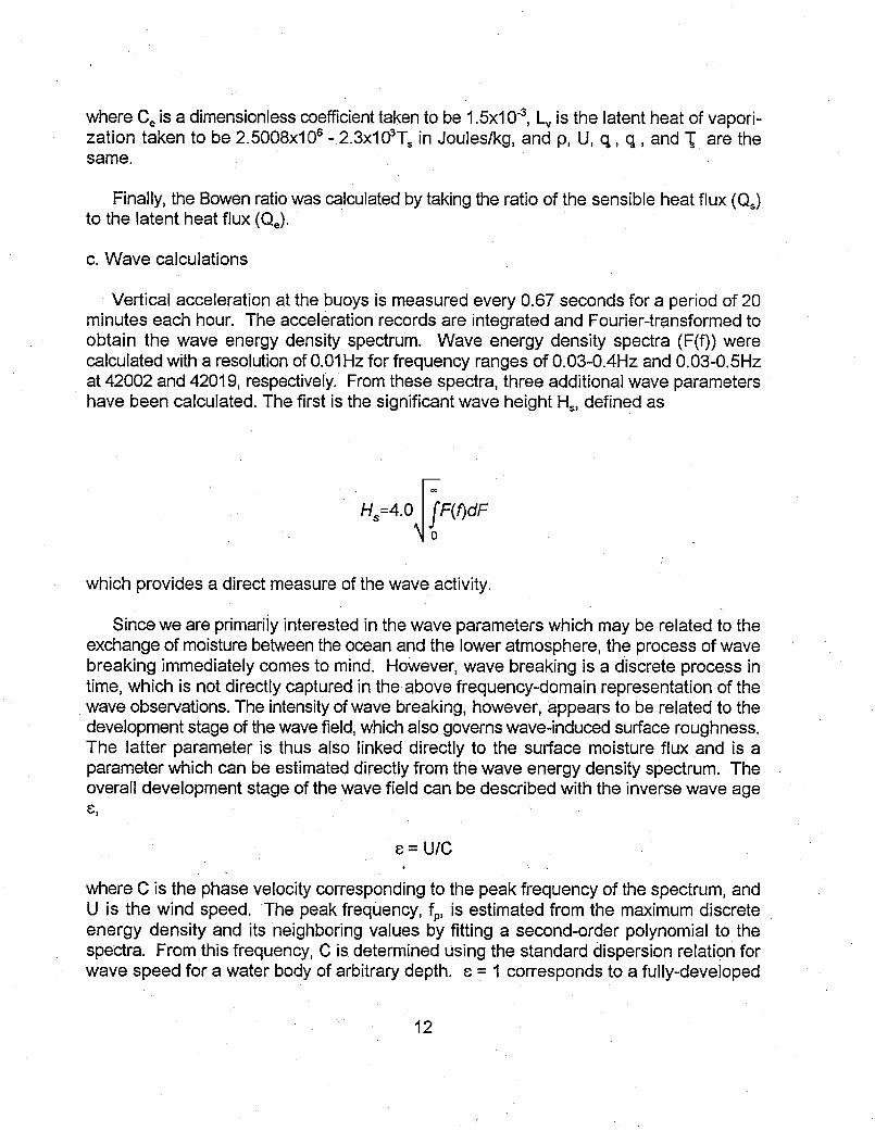
where Ce is a dimensionless coefficient taken to be 1.5x1 04, Lv is the latent heat of vapori-zation taken to be 2.5008x10⁶ - 2.3x1 '03Ts in Joules/kg, and p, U, q, q, and T are thesame.
Finally, the Bowen ratio was calculated by taking the ratio of the sensible heat flux (Qs)to the latent heat flux (Qe).
c. Wave calculations
Vertical acceleration at the buoys is measured every 0.67 seconds for a period of 20minutes each hour. The acceleration records are integrated and Fourier-transformed toobtain the wave energy density spectrum. Wave energy density spectra (F(f)) werecalculated with a resolution of 0.01Hz for frequency ranges of 0.03-0.4Hz and 0.03-0.5Hzat 42002 and 42019, respectively. From these spectra, three additional wave parametershave been calculated. The first is the significant wave height Hs, defined as
Hs=4.0 oF(f)dF
0
which provides a direct measure of the wave activity.
Since we are primarily interested in the wave parameters which may be related to theexchange of moisture between the ocean and the lower atmosphere, the process of wavebreaking immediately comes to mind. However, wave breaking is a discrete process intime, which is not directly captured in the above frequency-domain representation of thewave observations. The intensity of wave breaking, however, appears to be related to thedevelopment stage of the wave field, which also governs wave-induced surface roughness.The latter parameter is thus also linked directly to the surface moisture flux and is aparameter which can be estimated directly from the wave energy density spectrum. Theoverall development stage of the wave field can be described with the inverse wave age8,
= U/C
where C is the phase velocity corresponding to the peak frequency of the spectrum, andU is the wind speed. The peak frequency, fp, is estimated from the maximum discreteenergy density and its neighboring values by fitting a second-order polynomial to thespectra. From this frequency, C is determined using the standard dispersion relation forwave speed for a water body of arbitrary depth. 8 = 1 corresponds to a fully-developed
12
wind sea, i.e., a wind sea in equilibrium with the local wind sea, s > 1 corresponds togrowing wind waves and s < 1 corresponds to swell. The wave-induced contribution to thesurface stress is important for young waves only (e > 1).
Because the wave-induced roughness is primarily related to high-frequency waveenergy, another parameter of interest is the nondimensional energy of the high-frequencyflank of the spectrum a, also known as the 'Phillips' constant (Phillips 1958), where
fh
a = (2i) 4/g2 (fh f1 ) f F(f) f5dff
andf, = 1.5 * max(fP,fpM)
fh = max (2 .5 %fp, 2 .5*fpM,fma,)
fPM is the Pierson-Moskowitz frequency (Pierson and Moskowitz 1964) which is thefrequency for which s = 1 for a given wind speed, and fm. is the highest spectral frequencyobserved. a, is a measure of the small-scale roughness of the ocean surface, and,therefore, of the wave-induced surface stress. For a fully-developed sea, a ~ 0.01, andthe wave-induced stress again will be small. For larger a, active wave growth occurs, andwaves will contribute significantly to the surface stress. For smaller a, the contribution ofwaves to the surface stress is small. In such cases most of the wave energy can beattributed to swell. The limited range of frequencies for which the wave autospectra areobserved however, makes it impossible to evaluate a for low wind speeds and/or low waveheights. This parameter has only been evaluated for cases where the integralencompasses at least four discrete spectral densities. Note that a is still an indirectmeasure of the surface roughness, since the. actual roughness is primarily related tonear-capillary waves, well outside the range of the present wave observations.Furthermore, e and a generally behave similarly, since they can be considered aslarge-scale (e) or small-scale (a) estimates of the wave-induced surface roughness.
4. RESULTS
a. Validation
To provide a measure of validation for the observations of moisture acquired from thebuoy-mounted Rotronic humidity sensors, we have produced matchups of buoy data withmeasurements of boundary layer moisture acquired from selected ships and fixed plat-forms (primarily oil rigs) in the surrounding area. The majority of ship reports came fromtwo NOAA research vessels (NOAA Ships OREGON II and CHAPMAN) which were at sea
13
in the Gulf of Mexico during the study period. Each vessel was equipped with wet and drybulb thermometers and used standard WMO data collection and reporting procedures.
All of the reported moisture values obtained from the ships and fixed platforms wereconverted to specific humidities for direct comparison with the calculated specifichumidities from the buoys. The observations from each source were matched to within onehour in time and were made over a range of search radii from each of the buoys. Thesearch radii were increased in 25 km steps from 50 out to 300 km for each buoy. Thechoice of search radii was based on:
* (1) an e-folding correlation distance for specific humidity of - 800 km in the northernGulf of Mexico(see the following subsection for details), and
* (2) the need for adequate sample sizes.
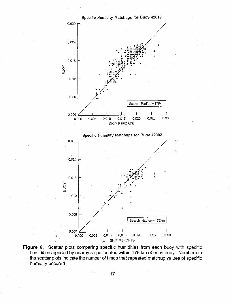
Figure 1 shows matchup circles for each buoy with search radii of 150 km. Scatter plotsfor matchups within a search radius of 175 km of each buoy are shown in Fig. 6. Biases,RMS differences, and correlations between the buoys and the ship reports are given inTable I for search radii of 50 to 300 km (in 50 km steps). The statistics becomerepeatable (i.e., stabilize) at sample sizes of the order of 300, which correspond to searchradii of 150 and 250 km for buoys 42019 and 42002, respectively. Although the buoymoistures on average tend to be slightly higher than the ship reports for the sensor on42019 (indicated by the positive biases), the opposite is true for the sensor on buoy 42002.The RMS differences are slightly higher and the correlations lower for the sensor on buoy42002. Overall, the correlations between the buoys and the ship reports are high; thus,these comparisons are generally favorable. However, a more conclusive validation studywould have required comparisons with reference standards located side-by-side with theRotronic sensors on each buoy.
Katsaros et al. (1994) recently conducted field tests of a number of humidity sensorsincluding the Rotronic MP-100 instrument. Hysteresis was found to occur for meanhumidities following high-moisture events for the Rotronic MP-100 instrument. Thegreatest differences between the Rotronic sensor and a reference psychrometer occurredat relative humidities less than 70%, particularly after periods of high relative humidity.The Rotronic sensor apparently required time to dry out after periods of high moisture.Finally, a bias of 8% between the Rotronic MP-100 and a reference psychrometer was notdue simply to a calibraton error but was attributed in part to hysteresis by the sensor.
To address the problem raised by Kataros et al., we first looked for periods of highrelative humidity in our data. Cumulative distributions of relative humidity for each buoyindicate that only about 8% of the data from either buoy have relative humidities thatexceed 90%, and only about 2% of the data exceed 95%. Overall, very few periods ofidentifiable rain occurred during the study period and those periods which could beidentified did not coincide precisely with any of our ship reports. To examine the
14

hysteresis problem adequately with our data would have required locating matchups thatoccurred within a narrow window of several hours following clearly-defined high-moisture(i.e., saturation) events and, as indicated, no such matchups were found. Ourcomparisons with the ship reports above, however, showed only small biases (3.6% for42019 and -4.1% for 42002). If hysteresis was a serious problem, we would haveexpected both biases to be positive (i.e., buoys to be higher than the ship reports). Thisresult, of course, was also influenced by the fact that high relative humidities (>-95%)were a relatively rare occurrence in our data. In summary, our data are not adequate toaddress the hysteresis problem raised by Katsaros et al. However, based on the limiteddata available, no evidence for a significant hysteresis problem could be found for theRotronic sensors deployed on buoys 42019 and 42002. Also, based on the results ofVisscher and Schurer (1985), Muller and Beekman (1987), and Hundermark (1989),hysteresis problems were not previously found with the Rotronic MP-100 instrument.
Table 1. Comparisons of specific humidities at NDBC buoys 42019 and 42002 with thosecomputed from nearby ship and fixed platform observations at various radii from eachbuoy.
Range (km) Sample Size Bias RMS CoefficientCoefficient
Station 42019
50 49 0.00043 0.00133 0.932
100 170 0.00059 0.00166 0.893
150 326 0.00089 0.00200 0.868
200 472 0.00081 0.00204 0.867
250 622 0.00073 0.00200 0.867
300 733 0.00067 0.00202 0.852
Station 42002
50 8 -0.00167 0.00220 0.780
100 33 -0.00132 0.00223 0.550
150 101 - -0.00146 0.00276 0.712
200 166 -0.00098 0.00237 0.728
250 333 -0.00084 0.00214 0.786
300 580 -0.00071 0.00224 0.780
15
b. Interpretation of the synoptic-scale variability
The variability of moisture within the marine boundary layer at buoys 42019 and 42002occurred on several time scales; however, the synoptic-scale variations in moisture standout as the dominant source of variability, particularly during September, October andNovember (Fig. 7). In order to examine this synoptic-scale activity in greater detail, westudied the appropriate surface weather maps.
On 17 June 1993, specific humidity decreased, and the surface heat fluxes increasedat both buoys, reflecting the influence of a tropical wave that formed near the YucatanPeninsula. Specific humidities remained relatively low for about 4 days, during which timethe tropical wave intensified becoming first a tropical depression and then Tropical StormArlene. Arlene moved to the NNW across the Gulf, approaching the buoys from the south.Arlene followed a path that took it west of buoy 42002, producing stronger responses interms of moisture and heat flux at 42002 than at 42019. The decrease in specific humidityat the surface conincided with decreases in SST of -2C, which were most likely producedby mixing in the oceanic surface layer.
On 26 September, specific humidity dropped suddenly at both buoys due to the firstsignificant cold front of the fall season. This system was composed of two fronts, a weakercool front closely followed by a more intense cold front. On 27 September, the first frontweakened significantly, while the second front passed the buoy at 42019 on its way toward42002. Later on the 27th, the dominant front passed 42002 with increasing'wind speedsand falling air and dew point temperatures. Dew point temperatures dropped by over 10Cat 42019 and by -5C at 42002, indicating that the air mass behind the front was not onlycold, but relatively dry. The impact of this frontal passage was clearly greater at 42019than it was at 42002 for all buoy parameters. By 30 September, the impact of the front hadpractically disappeared at both buoy locations. Moisture, in particular, was greatly affectedby the passage of this frontal system and, as a result, served as an excellent indicator offrontal behavior.
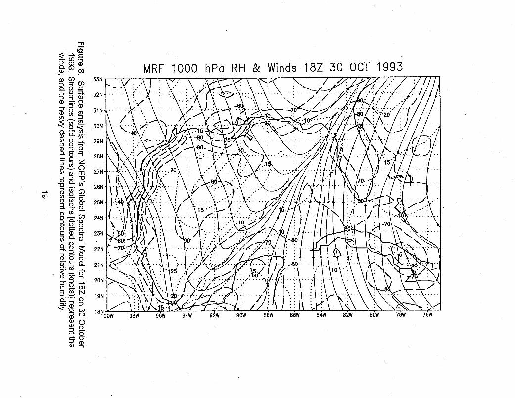
Starting on 21 October, a series of cold fronts began dropping down into the Gulf ofMexico and continued with some regularity through the end of November. Between 21 and29 October, two cold fronts entered the Gulf from the NW and within a day or two eachsystem had weakened sigificantly. On 30 October, a rapidly-moving, intense frontalsystem entered the Gulf from the north. The air mass behind this front was extremely coldand dry. Dew point temperatures at 42019 dropped to a low of 3.9C and at 42002 theyreached 6.7C as the center of high pressure behind the front continued to move south andinto the area where the buoys were located. Fig. 8 shows the surface analysis for 18Z on30 October from NMC's Aviation Model. This analysis clearly depicts the intensity of thisfrontal system at one point in its progression across the Gulf although it lags the buoyobservations by almost 12 hours and shows less drying behind the front (-80% observedvs. 90% from the analysis at 42019, and -75% observed vs. 90% at 42002). It took almost
16
Specific Humidity Matchups for Buoy 42019
* 2 4: /
* * 3422 2· .·,eMeM59 *2* *e023 M5923* ee *747M7 5**e5
2 2e56"9'6e 2* **e74;522 **2 * /3 * C*v3* *,
...2 422'30 : 2 .e*2 422 ef *.e* · 222
ee2* 23
!/ ·
2
I Search Radius=175km I
I I I I I I
0.005 0.010 0.015 0.020
SHIP REPORTS
0.025 0.030
Specific Humidity Matchups for Buoy
Z- 2.6 2232536 2* * 26,357 .*
/z .'*~~ ~ /3: -
* /. .C ·C C
C
/
/ / II I
0.005 0.010' 0.015 0.020
- SHIP REPORTS
0.025 0.030
Figure 6. Scatter plots comparing specific humidities from each buoy with specifichumidities reported by nearby ships located within 175 km of each buoy. Numbers inthe scatter plots indicate the number of times that repeated matchup values of specifichumidity occured.
17
0.030 r
0.024 F-
0.018 F-
0DM
0.012
0.006
/0.000 C
0.000
42002
0.030
0.024
0.018 -
0Dm
0.012 -
-7.~~~~~~0.006
n nnn I0.000uu 0.000
I Search Radius = 175km I
I I I
0
o (%J Cr.Y~~~~~~- -o,
o o Ci4C,~~~~~~~~~~~I(D~ ~ ~ ~ ~ ~ ~~F ~~- =C'_
II -- II
o H H~~~~~~L
1..
v n ~~~~~~~~~~~u v -jEC') ii
X Us - X EZ X s t9 X~,- , i'
::D ' ~ ~
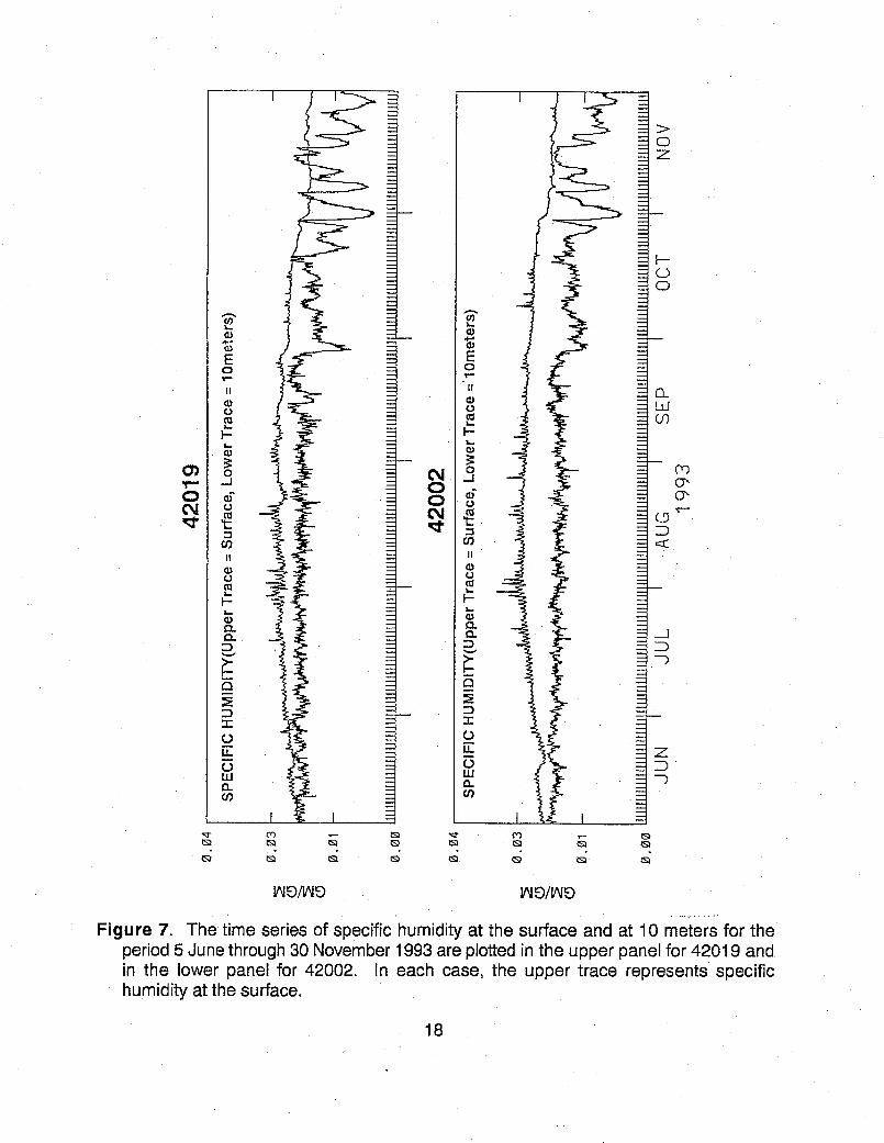
Figure 7. The time series of specific humidity at the surface and at 1 0 meters for theperiod 5 June through 30 November 1993 are plotted in the upper panel for 42019 andin the lower panel for 42002. In each case, the upper trace represents specifichumidity at the surface.
0 ~~~~~0'-=iF' · --
0.~~~~~~~~~~~~~~~~~~~~~~~~~~~~~~~~~~~~~~~~~~~~~~~~~~~.. 0..
Figure 7. The time series of specific humidity at the surface and at 10 meters for theperiod 5 June through 30 November 1993 are plotted in the upper panel for 42019 andin the lower panel for 42002. In each case, the upper trace represents specifichumidity at the surface.
18
-n'11
". O0s
-,- (co-':~ztD -0 Dt
tD r (.a)mC cn
(D = (nCD, m
~'©03
a) mo o .O03-.*
CD 0
o n M).
(D -OD Q vm
CD a
oD o -,CD
C"' ,,-n -
Q n r,
o o
(.o
Pr w
( CD -(0 (
030*('D<~~ 0
CD CL-
CDO
(D.. -oCD-
33N
32N
31 N
30N
29N '
28N
27N'
26N
25N
24N
23N
22N
21N
20N
19N
18N' -100W 98W 96W 94W 92W 90W 88W 86W 84W 82 BW 80W 78W /6W
MRF 1000 hPa RH & Winds 18Z 30 OCT 1993
..:[., K. :/. .
15...q. l- :'.-:3 X...... ..,/-5
~.-~~2 -
5 days for pre-frontal conditions to be re-established over the Gulf following the passageof this frontal system. On 6 November, another cold front dropped down into the northernGulf close behind the previous front. Although this frontal system was intense, it wasslightly weaker than the previous system.
Between 9 and 11 November, a small high-pressure system dropped down over thenorthern Gulf bringing slightly cooler and drier continental air with it, unlike the previousevents which were primarily frontal in nature. Between 17 and 30 November, three morecold fronts dropped down into the Gulf of Mexico causing air and dew-point temperaturesto drop significantly at the two buoy locations.
In summary, the events described above produced strong and well-defined signaturesin the moisture-related observations, emphasizing the importance of these data incharacterizing synoptic-scale variability in the near-surface marine environment.
c. Time series of environmental parameters
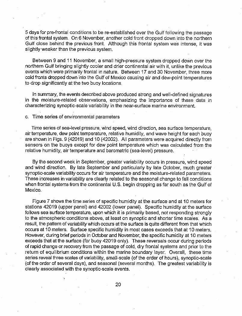
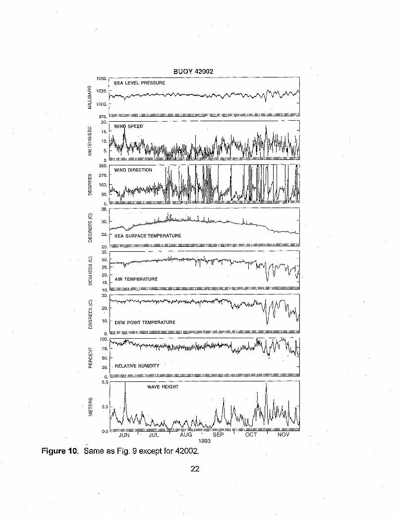
Time series of sea-level pressure, wind speed, wind direction, sea surface temperature,air temperature, dew point temperature, relative humidity, and wave height for each buoyare shown in Figs. 9 (42019) and 10 (42002). All parameters were acquired directly fromsensors on the buoys except for dew point temperature which was calculated from therelative humidity, air temperature and barometric (sea-level) pressure.
By the second week in September, greater variability occurs in pressure, wind speedand wind direction. By late September and particularly by late October, much greatersynoptic-scale variability occurs for air temperature and the moisture-related parameters.These increases in variability are clearly related to the seasonal change to fall conditionswhen frontal systems from the continental U.S. begin dropping as far south as the Gulf ofMexico.
Figure 7 shows the time series of specific humidity at the surface and at 10 meters forstations 42019 (upper panel) and 42002 (lower panel). Specific humidity at the surfacefollows sea surface temperature, upon which it is primarily based, not responding stronglyto the atmospheric conditions above, at least on synoptic and shorter time scales. As aresult, the pattern of variability which occurs at the surface is quite different from that whichoccurs at 10 meters. Surface specific humidity in most cases exceeds that at 10 meters.However, during brief periods in October and November, the specific humidity at 10 metersexceeds that at the surface (for buoy 42019 only). These reversals occur during periodsof rapid change or recovery from the passage of cold, dry frontal systems and prior to thereturn of equilibrium conditions within the marine boundary layer. Overall, these timeseries reveal three scales of variability, small-scale (of the order of hours), synoptic-scale(of the order of several days), and seasonal (several months). The greatest variability isclearly associated with the synoptic-scale events.
20
1050.
1025.
1000.
20.
15.
10.
5.
0.360.
270.
180.
90.
O.35.
BUOY 42019
30.
25.
20. 35.
30.
25.
20.-AIR TEMPERATURE15. '
10.30. .
20.10. DEW POINT TEMPERATURE
lUU.
75.
50.
25.
0.
JUN ' JUL AUG ' SEP.1993
I OCT ' NOV
Figure 9. Time series of hourly sea-level pressure, wind speed, wind direction, seasurface temperature, air temperature, dew point temperature, relative humidity andwave height are shown for the period 5 June through 30 November 1993, for the buoyat station 42019.
21
SEA LEVEL PRESSURE
L __Z<Xw
WIND SPEED .
, \~~~~~~~~~~~~~~~~~~~~~~~~~~~~~~~~~~~~~~~~~~~~~~~~~~~~~~~~~~~~~~~~~~~~~~~
Xh~~~~~~~....... y'
(12
O
Go
LU
_-J
2
LUww(12
:E
w
U)
w
F-
LU(12
LULU
C9
LU
0
UJ
LU
El(1LU
LUCC
CD
U)
Cc
0
CO
IC
5.(1LU
CE
- SEA SURFACE TEMPERATURE
- RELATIVE HUMIDITY
l III iii I IIIIIIIf llltl l f1 I iI[ I IiI II [1 III I IIIIIii i i i i III III 1 1 IIIIIII T II III III I II IIIIi111 1111 IIII I II IIIIIIII111111 iiiiii II I IIIIn III IIIIIII II I I II II II II IIIII I 11 IIIII
WAVE HEIGHT
Al .WS
CD
LUL-LU
2.5
W S75 ii i l 11 H ii i i ]1m F i H~1~H~1iI i ii i 1i i
n n
BUOY 42002
0 AIR TEMPERATURE10.-
DEW POINT TEMPERATURE
111R1E ~LAill~[l~,~ iTIVE ,l[~!~ HUM IDITY111, illll,,,,,,,I H I~lII~lIIIIIIIIlIII 11, q _lll ...!ll l ,I ,,,lll l MIIIIIII I I,,,I ....
1993
Figure 10. Same as Fig. 9 except for 42002.
22
SEA LEVEL PRESSURE
liii III lIIIlIIllIIIIIIIIIIII liii III�III III liii IIII�IIllII IllIllillIll I liii III liii III
1050.
CDn 1025.cD-j
-3 1000.
975.20.
0C 15.(o1Qn- 10.wC 5.
O.360.
CO 270.wwm 180.w 0 90.
O.35.
w
wCI)LLCD
30.
5.
0.5.
SEA SURFACE TEMPERATURE
_ ~~~~~~~~~~~~~~~~~~~~~~~~~~~~~~IIli 111 IFIIIIIIiiIii
(D 2LI0
23
' 3
UC 2
a: 2
" 1
1330.
CDaLULIJC-V_
0CD
20.
10.
0.100.
;- 75.zwo 50.Ccwa 25.
O.
co
FE
(r'wDt-CD
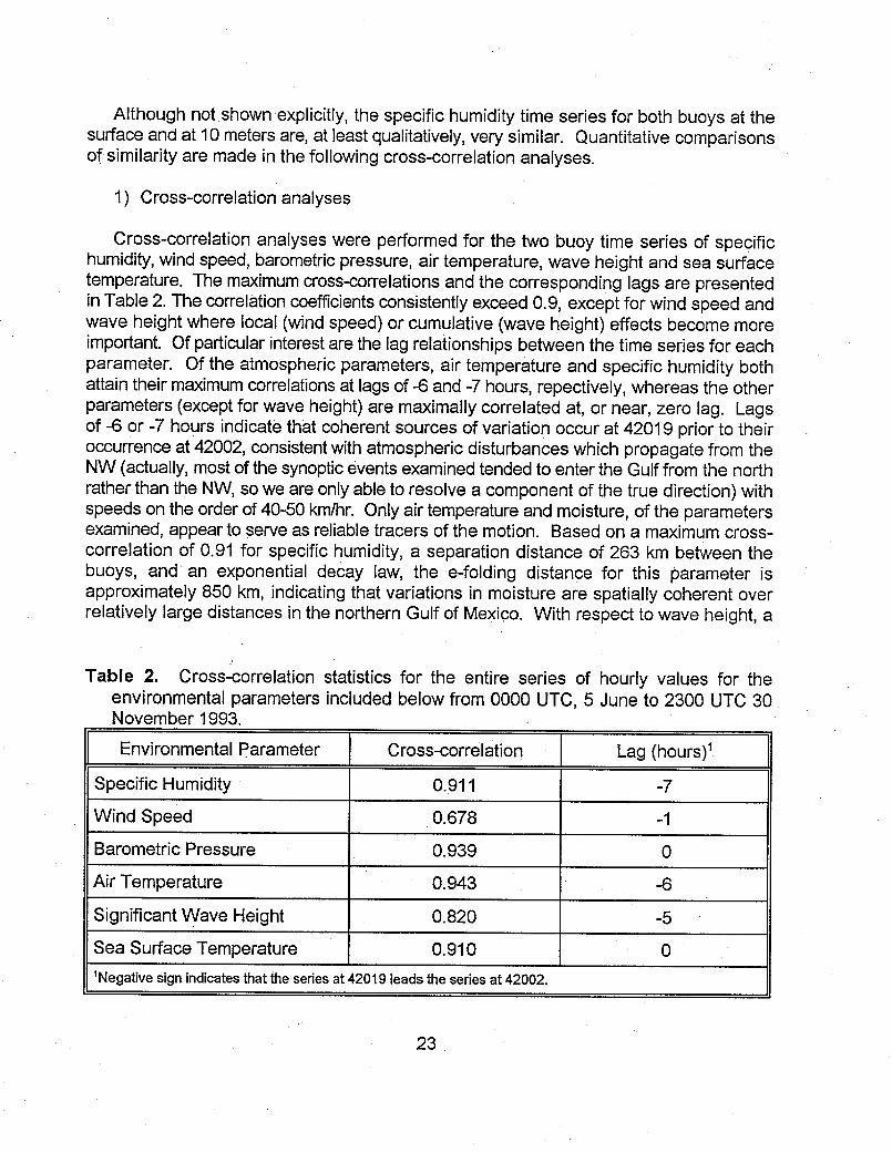
Although notshown explicitly, the specific humidity time series for both buoys at thesurface and at 10 meters are, at least qualitatively, very similar. Quantitative comparisonsof similarity are made in the following cross-correlation analyses.
1) Cross-correlation analyses
Cross-correlation analyses were performed for the two buoy time series of specifichumidity, wind speed, barometric pressure, air temperature, wave height and sea surfacetemperature. The maximum cross-correlations and the corresponding lags are presentedin Table 2. The correlation coefficients consistently exceed 0.9, except for wind speed andwave height where local (wind speed) or cumulative (wave height) effects become moreimportant. Of particular interest are the lag relationships between the time series for eachparameter. Of the atmospheric parameters, air temperature and specific humidity bothattain their maximum correlations at lags of -6 and -7 hours, repectively, whereas the otherparameters (except for wave height) are maximally correlated at, or near, zero lag. Lagsof -6 or -7 hours indicate that coherent sources of variation occur at 42019 prior to theiroccurrence at 42002, consistent with atmospheric disturbances which propagate from theNW (actually, most of the synoptic events examined tended to enter the Gulf from the northrather than the NW, so we are only able to resolve a component of the true direction) withspeeds on the order of 40-50 kmlhr. Only air temperature and moisture, of the parametersexamined, appear to serve as reliable tracers of the motion. Based on a maximum cross-correlation of 0.91 for specific humidity, a separation distance of 263 km between thebuoys, and an exponential decay law, the e-folding distance for this parameter isapproximately 850 km, indicating that variations in moisture are spatially coherent overrelatively large distances in the northern Gulf of Mexico. With respect to wave height, a
Table 2. Cross-correlation statistics for the entire series of hourly values for theenvironmental parameters included below from 0000 UTC, 5 June to 2300 UTC 30November 1993.
Environmental Parameter Cross-correlation [ Lag (hours)'
Specific Humidity 0.911 -7
Wind Speed 0.678 -1
Barometric Pressure 0.939 0
Air Temperature 0.943 -6
Significant Wave Height 0.820 -5
Sea Surface Temperature 0.910 0'Negative sign indicates that the series at 42019 leads the series at 42002.
23
lag of -5 hours indicates that the prevailing direction of propagation for surface gravitywaves in the northwestern Gulf of Mexico lies roughly between the southwest andnortheast quadrants.
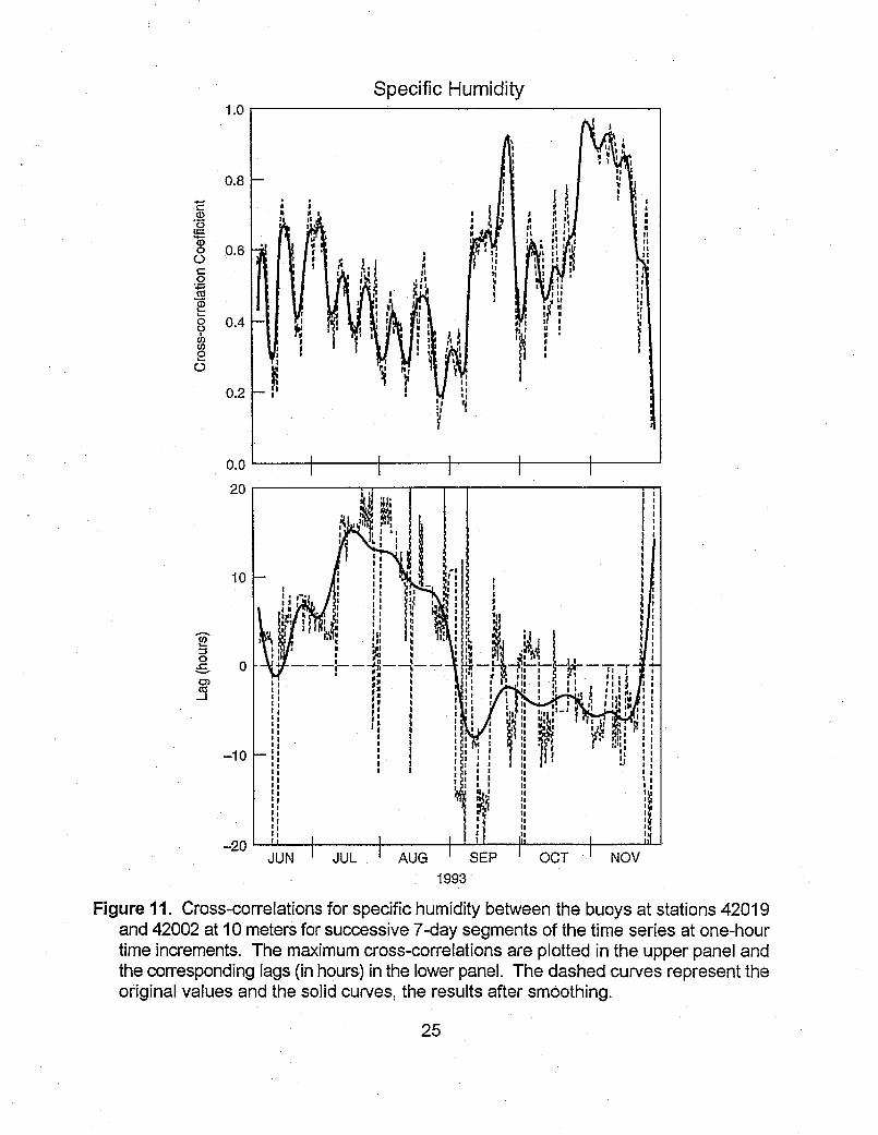
Successive cross-correlations for specific humidity were also calculated for 7-day (168-hour) periods, stepping through the data hour-by-hour. The results are displayed in Fig.11, where both the maximum cross-correlations (upper panel) and the corresponding lags(lower panel) are shown. The maximum correlations increase abruptly around 7September, and the lags change from mostly postive to essentially negative at this time,indicating that events prior to the first week in September generally arrived at 42002 beforethey arrived at 42019 and conversely thereafter. These significant changes in correlationstructure for specific humidity reflect a seasonal change in synoptic weather conditions inthe northern Gulf of Mexico. In particular, they imply that the prevailing weather patternsbecame more coherent and tended to enter the buoy domain from the North rather thanfrom the South after the first week in September (see subsection (d) for further details).
2) Spectral calculations
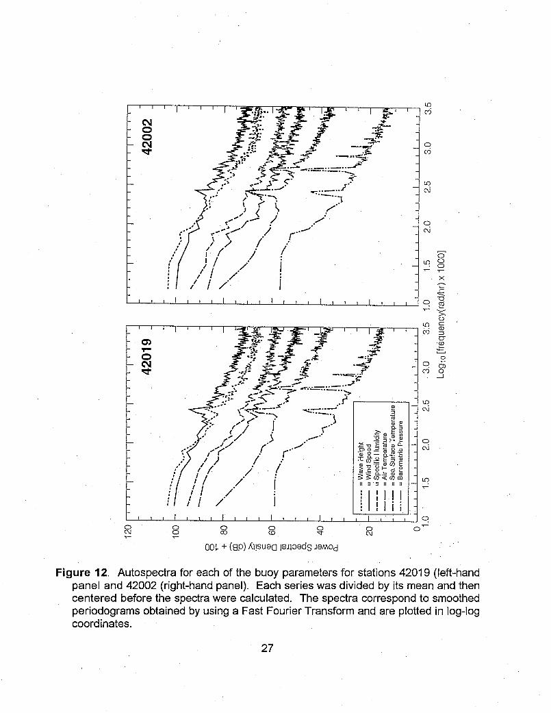
The time series of wave height, wind speed, specific humidity, air temperature, SST,and barometric pressure have also been subjected to spectral analysis in order to furtherexplore the character of the variability for the various buoy parameters. Prior to thespectral computations, each time series was normalized with respect to its mean; theresulting nondimensional series were then centered. The spectral computations wereperformed by first calculating raw spectral estimates using a Fast Fourier Transform andthen smoothing the resulting periodograms with a Parzen spectral window (IMSL Inc.1982). Figure 12 shows the autospectra for each of the buoy parameters (specifichumidity in place of relative humidity) plotted together for 42019 (left-hand panel) and42002 (right-hand panel).
All of the autospectra display similar negative slopes which are characteristic of mostgeophysical processes (the so-called "red noise" spectrum). Obvious spectral peaks occurat periods of 12 ("x"=2.73).and 24 ("x'=2.42) hours for barometric pressure, SST and airtemperature (but no obvious peak in air temperature at 12 hours for 42019), and lesserpeaks at 24 hours for wind speed. Weaker peaks can be detected at a period of -80hours ("x"=1.9) for most parameters, and most likely correspond to the passage ofsynoptic-scale events of atmospheric origin. At both buoy locations, the autospectra forwind speed and wave height are simliar (they actually cross at "x' = -2.1 in each cast),reflecting the close relationship that exists between the forcing and the response for theseparameters.
24
Specific Humidity1.0
0.8
0.6
0.4
0.2
0.0
20
10
-10
-10
I .'iL
AUG 1 SEP
1993
Figure 11. Cross-correlations for specific humidity between the buoys at stations 42019and 42002 at 10 meters for successive 7-day segments of the time series at one-hourtime increments. The maximum cross-correlations are plotted in the upper panel andthe corresponding lags (in hours) in the lower panel. The dashed curves represent theoriginal values and the solid curves, the results after smoothing.
25
'E
a)
0oC)00o
0
oo
'-z0c
.J
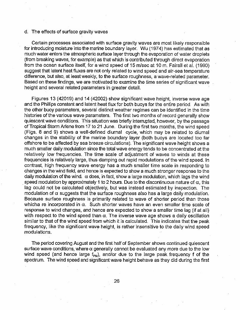
d. The effects of surface gravity waves
Certain processes associated with surface gravity waves are most likely responsiblefor introducing moisture into the marine boundary layer. Wu (1974) has estimated that asmuch water enters the atmospheric surface layer through the evaporation of water droplets(from breaking waves, for example) as that which is contributed through direct evaporationfrom the ocean surface itself, for a wind speed of 15 m/sec at 10 m. Fairall et al. (1990)suggest that latent heat fluxes are not only related to wind speed and air-sea temperaturedifference, but also, at least weakly, to the surface roughness, a wave-related parameter.Based on these findings, we are motivated to examine the time series of significant waveheight and several related parameters in greater detail.
Figures 13 (42019) and 14 (42002) show significant wave height, inverse wave ageand the Phillips constant and latent heat flux for both buoys for the entire period. As withthe other buoy parameters, several distinct weather regimes can be identified in the timehistories of the various wave parameters. The first two months of record generally showquiescent wave conditions. This situation was briefly interrupted, however, by the passageof Tropical Storm Arlene from 17 to 21 June. During the first two months, the wind speed(Figs. 8 and 9) shows a well-defined diurnal cycle, which may be related to diurnalchanges in the stability of the marine boundary layer (both buoys are located too faroffshore to be affected by sea breeze circulations). The significant wave height shows amuch smaller daily modulation since the total wave energy tends to be concentrated at therelatively low frequencies. The time scale of adjustment of waves to winds at thesefrequencies is relatively large, thus damping out rapid modulations of the wind speed. Incontrast, high frequency wave energy has a much smaller time scale in responding tochanges in the wind field, and hence is expected to show a much stronger response to thedaily modulation of the wind. a does, in fact, show a large modulation, which lags the windspeed modulation by approximately 1 to 2 hours. Due to the discontinuous nature of a, thislag could not be calculated objectively, but was instead estimated by inspection. Themodulation of a suggests that the surface roughness also has a large daily modulation.Because surface roughness is primarily related to wave of shorter period than thosewhicha re incorporated in a. Such shorter waves have an even smaller time scale ofresponse to wind changes, and hence are expected to show a smaller time lag (if at all)with respect to the wind speed than a. The inverse wave age shows a daily oscillationsimilar to that of the wind speed from which it is calculated. This indicates that the peakfrequency, like the significant wave height, is rather insensitive to the daily wind speedmodulations.
The period covering August and the first half of September shows continued quiescentsurface wave conditions, where a generally cannot be evaluated any more due to the lowwind speed (and hence large fpM), and/or due to the large peak frequency f of thespectrum. The wind speed and significant wave height behave as they did during the first
26
10
ICT~~~~~~~~~~~~~~~~~~~~C
L~~~~~~~~~~~~~~~~~~~~~~~~~Lo .. ' -~: .zr.
I- ~ ~ ~ * i/ ," ./ ! i r / I i f- ~~~~~~i f -*
"'D
C.
7 C) 0
,- ~ ~ - -..2--- .~J ... .C )
L'-~~~~~~~~~ ½~~~~~~~~~~~~~~~~
l ~ . :,: '": ~C,.~-.~ --,-..---...--..-'I :: ,-' ' . - I I I El
0~
-r. -CDO
00k + (9P) fqisueG( peJlsds Jemod "
Figure 12. Autospectra for each of the buoy parameters for stations 42019 (left-handpanel and 42002 (right-hand panel). Each series was divided by its mean and thencentered before the spectra were calculated. The spectra correspond to smoothedperiodograms obtained by using a Fast Fourier Transform and are plotted in log-logcoordinates.
27

420196.00
WAVE HEIGHT
- 3.00LLI
0.00
3.00
INVERSE WAVE AGE
1.50
0.00
0.02
0.01 WAVE ROUGHNESS
0.01
0.00
0.00
0.00 IlJ I
1000
800 LATENT HEAT FLUX
600
400
200
0
JUN JUL AUG SEP OCT . NOV
1993
Figure 13. Time series of significant wave height, wave age (inverse), wave roughness(a), and latent heat flux for the buoy at station 42019 for the period 5 June through 30November 1993.
28

6.00
C/)
LUI"-LIia: 3.00
0.00
3.00
1.50
0.00
n NO
42002
WAVE ROUGHNESS0.01
0.01
0.00 fil 1 II
0.00
1000
800 - LATENT HEAT FLUX
600
400
200
0
-200 il 11 lIt ii.iIf ,Ml till , , , I .,_,
1993
Figure 14. Same as Fig. 13 except for 42002.
29
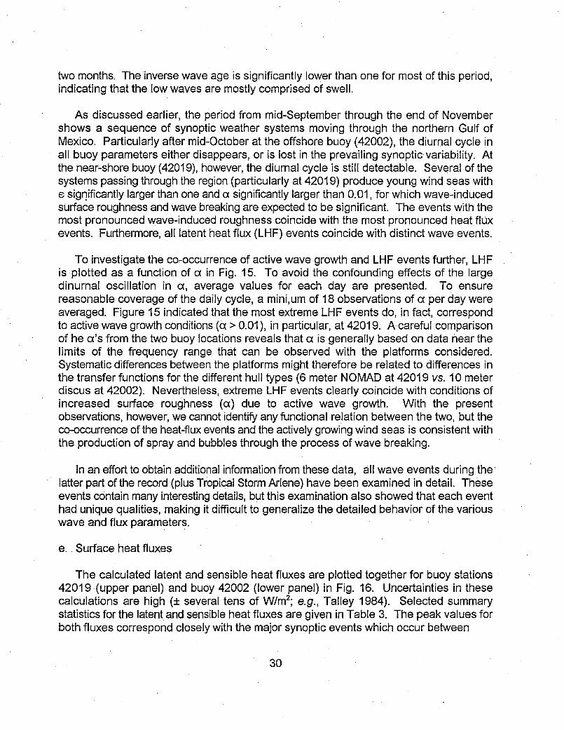
two months. The inverse wave age is significantly lower than one for most of this period,indicating that the low waves are mostly comprised of swell.
As discussed earlier, the period from mid-September through the end of Novembershows a sequence of synoptic weather systems moving through the northern Gulf ofMexico. Particularly after mid-October at the offshore buoy (42002), the diurnal cycle inall buoy parameters either disappears, or is lost in the prevailing synoptic variability. Atthe near-shore buoy (42019), however, the diurnal cycle is still detectable. Several of thesystems passing through the region (particularly at 42019) produce young wind seas withe significantly larger than one and a significantly larger than 0.01, for which wave-inducedsurface roughness and wave breaking are expected to be significant. The events with themost pronounced wave-induced roughness coincide with the most pronounced heat fluxevents. Furthermore, all latent heat flux (LHF) events coincide with distinct wave events.
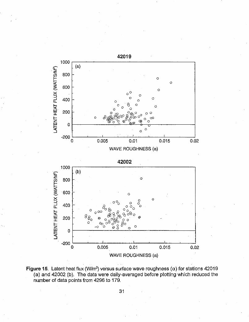
To investigate the co-occurrence of active wave growth and LHF events further, LHFis plotted as a function of a in Fig. 15. To avoid the confounding effects of the largedinurnal oscillation in a, average values for each day are presented. To ensurereasonable coverage of the daily cycle, a mini,um of 18 observations of a per day wereaveraged. Figure 15 indicated that the most extreme LHF events do, in fact, correspondto active wave growth conditions (a > 0.01), in particular, at 42019. A careful comparisonof he a's from the two buoy locations reveals that a is generally based on data near thelimits of the frequency range that can be observed with the platforms considered.Systematic differences between the platforms might therefore be related to differences inthe transfer functions for the different hull types (6 meter NOMAD at 42019 vs. 10 meterdiscus at 42002). Nevertheless, extreme LHF events clearly coincide with conditions ofincreased surface roughness (a) due to active wave growth. With the presentobservations, however, we cannot identify any functional relation between the two, but theco-occurrence of the heat-flux events and the actively growing wind seas is consistent withthe production of spray and bubbles through the process of wave breaking.
In an effort to obtain additional information from these data, all wave events during thelatter part of the record (plus Tropical Storm Arlene) have been examined in detail. Theseevents contain many interesting details, but this examination also showed that each eventhad unique qualities, making it difficult to generalize the detailed behavior of the variouswave and flux parameters.
e. Surface heat fluxes
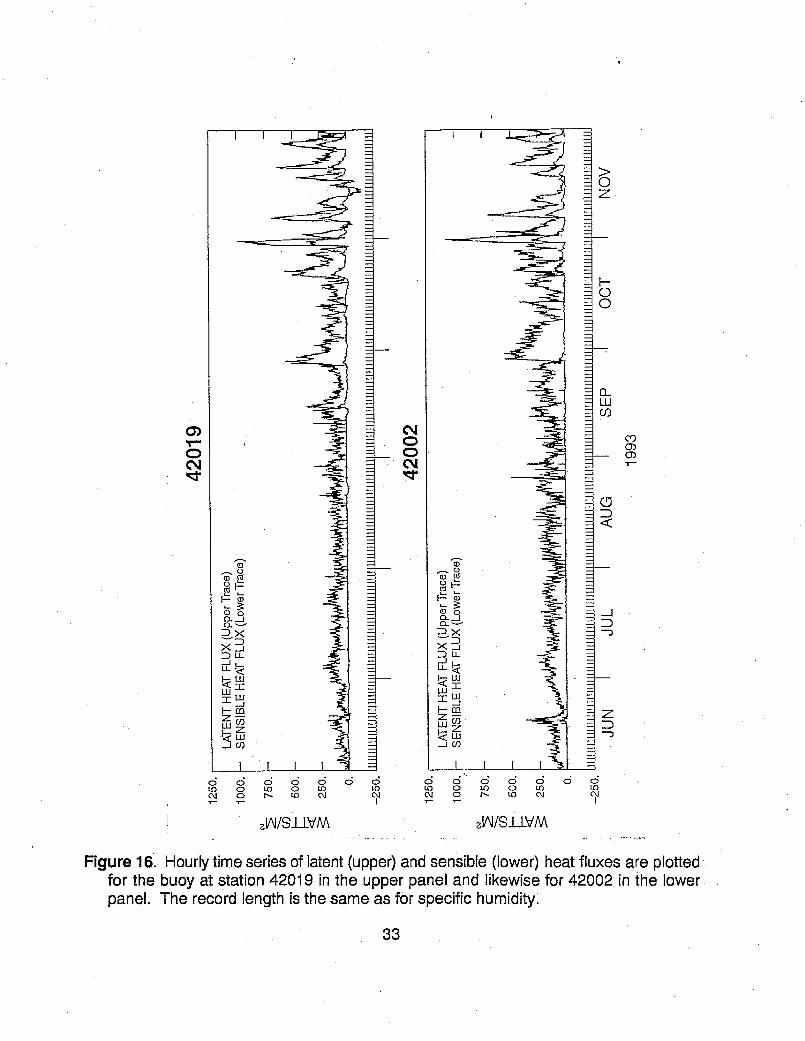
The calculated latent and sensible heat fluxes are plotted together for buoy stations42019 (upper panel) and buoy 42002 (lower panel) in Fig. 16. Uncertainties in thesecalculations are high (± several tens of W/m2; e.g., Talley 1984). Selected summarystatistics for the latent and sensible heat fluxes are given in Table 3. The peak values forboth fluxes correspond closely with the major synoptic events which occur between
30
42019
0.01
WAVE ROUGHNESS (a)
42002
0.01
WAVE ROUGHNESS (a)
Figure 15. Latent heat flux (W/m 2 ) versus surface wave roughness (a) for stations 42019(a) and 42002 (b). The data were daily-averaged before plotting which reduced thenumber of data points from 4296 to 179.
31
1000
800
600
400
200
0
-200
x1-I
LIL
zwHR-j
(a)
00
0o00 00
0 0
o0
0 0 0 000kr co C6 0O O
00I I . I I I
0 0.005 0.015
1000
0.02
800
600
CDrx-JLL
LUHIzUJ_J
- (b)
0
0
.00 0 0 00608O00 0 0
- 000~0 03(6~ 0
- 88. 0 _ oI I oo I Io-0 *0 0 0
rI II,
400
200
0
-2000 0.005 0.015 0.02
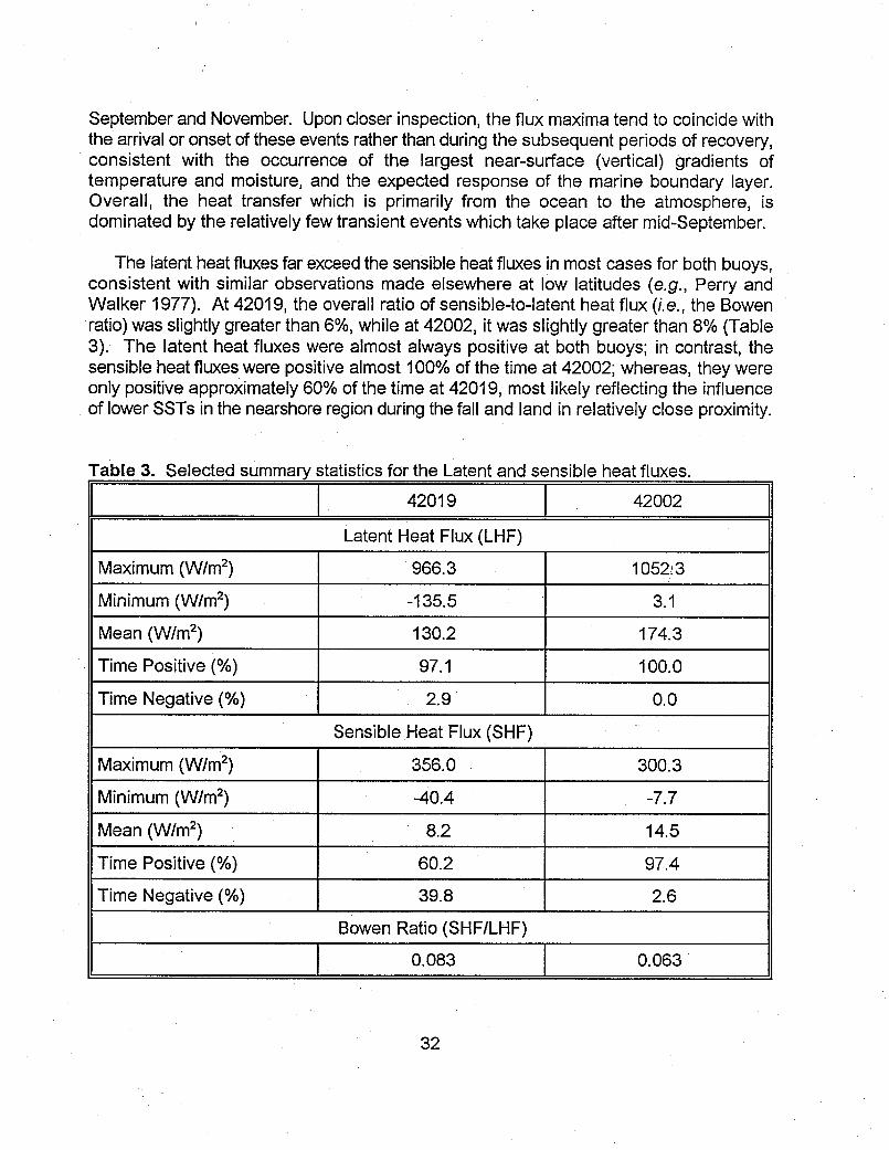
September and November. Upon closer inspection, the flux maxima tend to coincide withthe arrival or onset of these events rather than during the subsequent periods of recovery,consistent with the occurrence of the largest near-surface (vertical) gradients oftemperature and moisture, and the expected response of the marine boundary layer.Overall, the heat transfer which is primarily from the ocean to the atmosphere, isdominated by the relatively few transient events which take place after mid-September.
The latent heat fluxes far exceed the sensible heat fluxes in most cases for both buoys,consistent with similar observations made elsewhere at low latitudes (e.g., Perry andWalker 1977). At 42019, the overall ratio of sensible-to-latent heat flux (i.e., the Bowenratio) was slightly greater than 6%, while at 42002, it was slightly greater than 8% (Table3). The latent heat fluxes were almost always positive at both buoys; in contrast, thesensible heat fluxes were positive almost 100% of the time at 42002; whereas, they wereonly positive approximately 60% of the time at 42019, most likely reflecting the influenceof lower SSTs in the nearshore region during the fall and land in relatively close proximity.
Table 3. Selected summary statistics for the Latent and sensible heat fluxes.
_J 42019 42002
Latent Heat Flux (LHF)
Maximum (W/m 2) 966.3 1052!3
Minimum (WIm 2) -135.5 3.1
Mean (W/m 2) 130.2 174.3
Time Positive (%) 97.1 100.0
Time Negative (%) 2.9 0.0
Sensible Heat Flux (SHF)
Maximum (W/m2) 356.0 300.3
Minimum (W/m 2) -40.4 -7.7
Mean (W/m 2)8.2 14.5
Time Positive (%) 60.2 97.4
Time Negative (%) 39.8 2.6
Bowen Ratio (SHFILHF)
I 0.083 0.063
32
CY)LD O ( O %0 J0 U) CY)
0~~~~~~~~:D
Xl~~~ -rD~~~~~~~~~1-0.
D _
M~DLLI DL
zA/S-LiVAA zn/SI- &
Figure 16. Hourly time series of latent (upper) and sensible (lower) heat fluxes are plottedfor the buoy at station 42019 in the upper panel and likewise for 42002, in the lowerpanel. The record length is the same as for specific humidity.-
w_-
Z U)Z
c'
WlAIISLL VM A/_LM
Figure 16. Hourly time series of latent (upper) and sensible (lower) heat fluxes are plottedfor the buoy at station 42019 in the upper panel and likewise for 42002 in the lowerpanel. The record length is the same as for specific humidity.
33
The latent heat fluxes and the sensible heat fluxes for both buoys, when plottedtogether, are very similar and thus highly correlated (not shown). Plots of the Bowen ratiotime series (ratio of the sensible-to-latent heat fluxes)t were also produced. The Bowenratio was generally small (< -0.1); however, occasional isolated spikes (i.e., transientextreme values) occurred that were usually positive and exceeded 0.5 in several cases.These spikes occurred more frequently at 42002 and were distributed across the entirerecord; there were fewer spikes at 42019 and those that occurred, were observed onlyduring October and November.
5. SUMMARY AND CONCLUSIONS
The overall reliability of the Rotronic MP-100 humidity sensors, which have beendeployed on various NDBC buoys over the past five years, has improved significantlysince 1989 when they were first considered for possible long-term deployment on fixedplatforms at sea.
Over the approximate six-month period that the Rotronic sensor installed on the buoyat station 42019 was deployed, its calibration remained within the accuracy limits set bythe WMO. The Rotronic sensor installed on the buoy at station 42002 has been operatingcontinuously since its deployment in June 1993 (a period of more than 26 months).
Katsaros et al. (1994) have recently reported that the Rotronic sensor experienceshysteresis following periods of high mosture. Our observations did not'permit us toexamine this question in detail. In this regard, our results may not be representative of theresults that might have been obtained elsewhere such as along the coast of Califroniawhere fog is frequently encountered. However, problems associated with hysteresis forthe Rotronic sensor have not been reported elsewhere. Clearly, this issue needs furtherclarification. If hysteresis turns out to be a continuing problem that cannot be easilysolved, moisture data from this instrument will most likely be unsuitable for research;however, it should still be of considerable value for operational applications.
During the six-month period of this study, most of the synoptic-scale variability that wasencountered occurred after the first week in September and was due to the arrival offrontal systems with cold, dry air behind them that dropped down into the Gulf of Mexicofrom the continental U.S. One exception occurred in June when Tropical Storm Arlenemoved NNW across the Gulf strongly influencing the moisture field in the vicinity of thebuoys. In summary, the moisture-related parameters acquired at the buoys (specifichumidity in particular) were highly sensitive in all cases to the various synoptic-scaleevents and to the seasonal variability that took place in the marine boundary layer duringthe period of this study.
Observations at each of the buoys acquired during this study were used to constructtime series of specific humidity; in turn, from these and other supporting data, the surface
34
fluxes of latent and sensible heat were calculated. The time series of specific humidity ata height of 10 meters reveal three primary scales of variability:
* small-scale (of the order of hours),• synoptic-scale (-several days), and* seasonal (several months).
The synoptic-scale variability was clearly dominant and event-like in character; also, itoccurred primarily during September, October and November.
A cross-correlation analysis between the buoys (for a separation distance of 263 km)for specific humidity and the other buoy parameters (at 10 meters) indicated:
* (1) all parameters were highly-correlated (> 0.9) except for wind speed,* (2) the e-folding correlation distance for specific humidity was at least 800 km, and* (3) specific humidity and air temperature both served as tracers of the motion
associated with propagating atmospheric disturbances.
A more detailed cross-correlation analysis of the specific humidity time series revealed amajor change in correlation structure that occurred during the first week in Septemberindicating that weather patterns became more coherent and tended to enter the northernGulf of Mexico from the North rather than from the South, as they tended to prior to thistime.
Autospectra of the various buoy measurements revealed strong diurnal and semidiurnalvariability for barometric pressure and SST and lesser variability at these periods for airtemperature and wind speed. Also, weaker synoptic-scale variability was evident atperiods of 3-4 days for most of the atmospheric parameters.
Analysis of the surface wave observations from each buoy included calculations ofwave age and surface roughness. The results are consistent with enhanced moisturetransfer between the ocean and the marine boundary layer during periods of high latentheat flux.
The surface fluxes of latent and sensible heat were dominated by the synoptic eventswhich took place after mid-September. Sharp, positive maxima in these fluxes coincidedwith the arrival of these transient events in the northern Gulf of Mexico. The predominantdirection of heat transfer for both fluxes was from the ocean to the atmosphere (-100% ofthe time for the latent heat fluxes, and 60 and 97% of the time for the sensible heat fluxesfor buoys 42019 and 42002, respectively). The latent heat fluxes usually far exceeded thesensible heat fluxes as indicated by mean Bowen ratios of 6.3% at buoy 42019 and 8.3%at buoy 42002.
35
ACKNOWLEDGEMENTS
We take this opportunity to thank Bhavani Balashubramaniyan and Rachel Teboullefor constructing many of the figures contained in the text. We thank Steve Lord forcreating figure 8 and for reviewing the text. We thank Lech Lobocki for providing technicalassistance during the course of this study. Finally, we thank D. B. Rao, Ted Mettlach, EricMeindl and Ed Michelena for providing reviews fo the text.
REFERENCES
Coantic, M., and C. A. Friehe, 1980: Slow-response humidity sensors. Air-Sea Interaction,In Instruments and Methods (F. Dobson, L. Hasse, and R. Davis, eds.) Plenum Press,New York and London, pp 399-411.
Crane, J., and D. Boole, 1988: Thin film humidity sensors: a rising technology. Sensors,5, 32-35.
Crescenti, G. H., R. E. Payne, and R. A. Weller, 1990: Improved meteorologicalmeasurements from buoys and ships (IMET): preliminary comparison of humiditysensors. Woods Hole Tech. Rep. WHOI-90-18, Woods Hole OceanographicInstitution, 57 pp.
Fairall, C. W., J. B. Edson, and M. A. Miller, 1990: Heat fluxes, whitecaps, and sea spray.Surface Waves and Fluxes, Volume 1 - Current Theory (G.L. Geernaert, and W. J.Plant, eds.) Kluwer Academic Publishers, Dordrecht, pp 173-208.
Friehe, C. A., and K. F. Schmitt, 1976: Parameterization of air-sea interface fluxes ofsensible heat and moisture by the bulk aerodynamic formulas. J. Phys. Oceanogr., 6,801-809.
Gill, A. E., 1982: Atmosphere-Ocean Dynamics, International Geophysics Series, Volume30. New York: Academic Press, 662 pp.
Hundermark, B. W., 1989: Field evaluation of the Rotronic humidity sensor and theimpulsphysik visibility sensor. Proceedings, Conference and Exposition on MarineData Sysytems, New Orleans, Louisiana, Marine Technology Society, 81-85.
IMSL, Inc., 1982: IMSL Library Reference Manual, ed. 8, vol. 2, Houston, Texas.
Katsaros, K B., J. DeCosmo, R. J. Lind, R. J. Anderson, S. D. Smith, R. Kraan, W. Oost,K. Uhlig, P. G. Mestayer, S. E. Larsen, M. H. Smith, and G. de Leeuw, 1994:Measurements of humidity and temperature in the marine environment during theHEXOS main experiment. J. Atmos. Oceanic Technol., 11, 964-981.
36
Kraus, E. B., 1972: Atmosphere - Ocean Interaction, Clarendon Press, Oxford, 275 pp.
Muller, S. A. and P. J. Beekman, 1987: A test of commercial humidity sensors for use atautomatic weather stations. J. Atmos. Oceanic Technol., 4, 731-735.
Perry, A. H. and J. M. Walker, 1977: The Ocean - Atmosphere System, Longman, NewYork, 160 pp.
Phillips, O. M., 1958: The equilibrium range in the spectrum of wind-generated waves. J.Fluid Mech., 4, 426434.
Pierson, W. J. and L. Moskowitz, 1964: A proposed spectral form for fully-developed windseas based on the similarity theory of S. A. Kitaigorodskii. J. Geophys. Res., 69: 5181-5190.
Roll, H. U., 1965: Physics of the Marine Atmosphere, International Geophysics Series,Volume 7, Academic Press, New York, 426 pp.
Semmer, S. R., 1987: Evaluation of a capacitance humidity sensor. Sixth Symposium onMeteorological Observations and Instrumentation, New Orleans, Louisiana, AmericanMeteorological Society, 223-225.
Talley, L. D., 1984: Meridional heat transport in the Pacific ocean. J. Phys. Oceanogr., 14231- 241.
Visscher, G. J. W. and K. Schurer, 1985: Some research on the stability of severalcapacitive thin film (polymer) humidity sensors in practice. Proceedings, InternationalSymposium on Moisture and Humidity, Washington, D.C., Instrument Society ofAmerica, 515-523.
Van der Meulen, J. P., 1988: On the need of appropriate filter techniques to be consideredusing electrical humidity sensors. Proc. WMO Technical Conf. on Instruments andMethods of Observation (TECO-1988), Leipzig, Germany, WMO, 55-60.
World Meteorological Organization, 1983: Measurement of Atmospheric humidity. Guideto Meteorological Instruments and Methods of Observation, Fifth Edition. WMO No.8.
Wu, J., 1974: Evaporation due to spray. J. Geophys. Res., 79, 4107-4109.
37
OPC CONTRIBUTIONS (Cont.)
No. 21. Breaker, L. C., 1989: El Nino and Related Variability in Sea-Surface Temperature Along the Central California Coast.PACLIM Monograph of Climate Variability of the Eastern North Pacific and Western North America, GeophysicalMonograph 55, AGU, 133-140.
No. 22. Yu, T. W., D. C. Esteva, and R. L. Teboulle, 1991: A Feasibility Study on Operational Use of Geosat Wind and WaveData at the National Meteorological Center. Technical Note/NMC Office Note No. 380, 28pp.
No. 23. Burroughs, L. D., 1989: Open Ocean Fog and Visibility Forecasting Guidance System. Technical Note/NMC OfficeNote No. 348, 18pp.
No. 24. Gerald, V. M., 1987: Synoptic Surface Marine Data Monitoring. Technical Note/NMC Office Note No. 335, 10pp.
No. 25. Breaker, L. C., 1989: Estimating and Removing Sensor Induced Correlation form AVHRR Data. Journal ofGeophysical Reseach, 95, 9701-9711.
No. 26. Chen, H. S., 1990: Infinite Elements for Water Wave Radiation and Scattering. International Journal for NumericalMethods in Fluids11, 555-569.
No. 27. Gemmill, W. H., T. W. Yu, and D. M. Feit, 1988: A Statistical Comparison of Methods for Determining Ocean SurfaceWinds. Journal of Weather and Forecasting. 3, 153-160.
No. 28. Rao. D. B., 1989: A Review of the Program of the Ocean Products Center. Weather and Forecasting. 4, 427-443.
No. 29. Chen, H. S., 1989: Infinite Elements for Combined Diffration and Refraction. Conference Preprint, SeventhInternational Conference on Finite Element Methods Flow Problems Huntsville Alabama, 6pp.
No. 30. Chao, Y. Y., 1989: An Operational Spectral Wave Forecasting Model for the Gulf of Mexico. Proceedings of 2ndInternational Workshop on Wave Forecasting and Hindcasting, 240-247.
No. 31. Esteva, D. C., 1989: Improving Global Wave Forecasting Incorporating Altimeter Data. Proceedings of 2ndInternational Workshop on Wave Hindcasting and Forecasting,Vancouver, B.C., April 25-28, 1989, 378-384.
No. 32. Richardson, W. S., J. M. Nault, and D. M. Feit, 1989: Computer-Worded Marine Forecasts. Preprint, 6th Symp. onCoastal Ocean Management Coastal Zone 89, 4075-4084.
No. 33. Chao, Y. Y., and T. L. Bertucci, 1989: A Columbia River Entrance Wave Forecasting Program Developed at the OceanProducts Center. Techical Note/NMC Office Note 361.
No. 34. Burroughs, L. D., 1989: Forecasting Open Ocean Fog and Visibility. Preprint, 1 1th Conference on Probability andStatisitcs, Monterey, Ca., 5pp.
No. 35. Rao, D. B., 1990: Local and Regional Scale Wave Models. Proceeding (CMM/WMO) Technical Conference on Waves,WMO, Marine Meteorological of Related Oceanographic Activities Report No. 12, 125-138.
No. 36. Burroughs, L.D., 1991: Forecast Guidance for Santa Ana conditions. Technical Procedures Bulletin No. 391, 1 lpp.
No. 37. Burroughs, L. D., 1989: Ocean Products Center Products Review Summary. Technical Note/NMC Office Note No.359.29pp.
No. 38. Feit, D. M., 1989: Compendium of Marine Meteorological and Oceanographic Products of the Ocean Products Center(revision 1). NOAA Technical Memo NWS/NMC 68.
No. 39. Esteva, D. C., and Y. Y. Chao, 1991: The NOAA Ocean Wave Model Hindcast for LEWEX. Directional Ocean WaveSpectra, Johns Hopkins University Press, 163-166.
No. 40. Sanchez, B. V., D. B. Rao, and S. D. Steenrod, 1987: Tidal Estimation in the Atlantic and Indian Oceans, 3° x 3°
Solution. NASA Technical Memorandum 87812, 18pp.
OPC CONTRIBUTIONS (Cont.)
No. 41. Crosby, D. S., L. C. Breaker, and W. H. Gernmill, 1990: A Defintion for Vector Correlation and its Application toMarine Surface Winds. Technical Note/NMC Office Note No. 365, 52pp.
No. 42. Feit, D. M., and W. S. Richardson, 1990: Expert System for Quality Control and Marine Forecasting Guidance.Preprint, 3rd Workshop Operational and Metoerological. CMOS, 6pp.
No. 43. Gerald, V. M., 1990: OPC Unified Marine Database Verification System. Technical Note/NMC Office Note No. 368,1 4pp.
No. 44. Wohl, G. M., 1990: Sea Ice Edge Forecast Verification System. National Weather Association Digest, (submitted)
No. 45. Feit, D. M., and J. A. Alpert, 1990: An Operational Marine Fog Prediction Model. NMC Office Note No. 371, 18pp.
No. 46. Yu, T. W., and R. L. Teboulle, 1991: Recent Assimilation and Forecast Experiments at the National MeteorologicalCenter Using SEASAT-A Scatterometer Winds. Technical Note/NMC Office Note No. 383, 45pp.
No. 47. Chao, Y. Y., 1990: On the Specification of Wind Speed Near the Sea Surface. Marine Forecaster Training Manual.
No. 48. Breaker, L. C., L. D. Burroughs, T. B. Stanley, and W. B. Campbell, 1992: Estimating Surface Currents in the SlopeWater Region Between 37 and 41°N Using Satellite Feature Tracking. Technical Note, 47pp.
No. 49. Chao, Y. Y., 1990: The Gulf of Mexico Spectral Wave Forecast Model and Products. Technical Procedures Bulletin
No. 381, 3pp.
No. 50. Chen, H. S., 1990: Wave Calculation Using WAM Model and NMC Wind. Preprint, 8th ASCE EngineeringMechanical Conference, 1, 368-372.
No. 51. Chao, Y. Y., 1990: On the Transformation of Wave Spectra by Current and Bathymetry. Preprint, 8th ASCEEngineering Mechnical Conference, 1,333-337.
No. 52. WAS NOT PUBLISHED
No. 53. Rao, D. B., 1991: Dynamical and Statistical Prediction of Marine Guidance Products. Proceedings, IEEE ConferenceOceans 91, 3, 1177-1180.
No. 54. Gemmill, W. H., 1991: High-Resolution Regional Ocean Surface Wind Fields. Proceedings, AMS 9th Conference onNumerical Weather Prediction, Denver, CO, Oct. 14-18, 1991, 190-191.
No. 55. Yu, T. W., and D. Deaven, 1991: Use of SSM/I Wind Speed Data in NMC's GDAS. Proceedings, AMS 9th Conferenceon Numerical Weather Prediction, Denver, CO, Oct. 14-18, 1991, 416-417.
No. 56. Burroughs, L. D., and J. A. Alpert, 1993: Numerical Fog and Visiability Guidance in Coastal Regions. TechnicalProcedures Bulletin. No.398, 6pp.
No. 57. Chen, H. S., 1992: Taylor-Gelerkin Method for Wind Wave Propagation. ASCE 9th Conf. Eng. Mech. (in press)
No. 58. Breaker, L. C., and W. H. Gernmill, and D. S. Crosby, 1992: A Technique for Vector Correlation and its Application toMarine Surface Winds. AMS 12th Conference on Probability and Statistics in the Atmospheric Sciences, Toronto,Ontario, Canada, June 22-26, 1992.
No. 59. Yan, X.-H., and L. C. Breaker, 1993: Surface Circulation Estimation Using Image Processing and Computer VisionMethods Applied to Sequential Satellite Imagery. Photogrammetric Engineering and Remote Sensing, 59, 407-413.
No. 60. Wohl, G., 1992: Operational Demonstration of ERS-1 SAR Imagery at the Joint Ice Center. Proceeding of the MTS 92- Global Ocean Partnership, Washington, DC, Oct. 19-21, 1992.
OPC CONTRIBUTIONS (Cont.)
No. 61. Waters, M. P., Caruso, W. H. Gemmill, W. S. Richardson, and W. G. Pichel, 1992: An Interactive Information andProcessing System for the Real-Time Quality Control of Marine Meteorological Oceanographic Data. Pre-print 9thInternational Conference on Interactive Information and Processing System for Meteorology, Oceanography andHydrology, Anaheim, CA, Jan. 17-22, 1993.
No. 62. Breaker, L. C., and V. Krasnopolsky, 1994: The Problem of AVHRR Image Navigation Revisited. Int. Journal ofRemote Sensing, 15, 979-1008.
No. 63. Crosby, D. S., L. C. Breaker, and W. H. Gemmill, 1993: A Proposed Definition for Vector Correlation in Geophysics:Theory and Application. Journal of Atmospheric and Ocean Technology, 10, 355-367.
No. 64. Grumbine, R., 1993: The Thermodynamic Predictability of Sea Ice. Journal of Glaciology, 40, 277-282, 1994.
No. 65. Chen, H. S., 1993: Global Wave Prediction Using the WAM Model and NMC Winds. 1993 International Conferenceon Hydro Science and Engineering, Washington, DC, June 7 - 11, 1993. (submitted)
No. 66. WAS NOT PUBLISHED
No. 67. Breaker, L. C., and A. Bratkovich, 1993: Coastal-Ocean Processes and their Influence on the Oil Spilled off SanFrancisco by the M/V Puerto Rican. Marine Environmental Research, 36, 153-184.
No. 68. Breaker, L. C., L. D. Burroughs, J. F. Culp, N. L. Gunasso, R. Teboulle, and C. R. Wong, 1993: Surface and Near-Surface Marine Observations During Hurricane Andrew. Technical Note/NMVC Office Note #398, 41pp.
No. 69. Burroughs, L. D., and R. Nichols, 1993: The National Marine Verification Program - Concepts and Data Management,Technical Note/NMC Office Note #393, 21pp.
No. 70. Gemmill, W. H., and R. Teboulle, 1993: The Operational Use of SSM/I Wind Speed Data over Oceans. Pre-print 13thConference on Weather Analyses and Forecasting, AMS Vienna, VA., August 2-6, 1993, 237-238.
No. 71. Yu, T.-W., J. C. Derber, and R. N. Hoffman, 1993: Use of ERS-1 Scatterometer Backscattered Measurements inAtmospheric Analyses. Pre-print 13th Conference on Weather Analyses and Forecasting, AMS, Vienna, VA., August2-6, 1993, 294-297.
No. 72. Chalikov, D. and Y. Liberman, 1993: Director Modeling of Nonlinear Waves Dynamics. J. Physical, (To besubmitted).
No. 73. Woiceshyn, P., T. W. Yu, W. H. Gemmill, 1993: Use of ERS-1 Scatterometer Data to Derive Ocean Surface Winds atNMC. Pre-print 13th Conference on Weather Analyses and Forecasting, AMS, Vienna, VA, August 2-6, 1993, 239-240.
No. 74. Grumbine, R. W., 1993: Sea Ice Prediction Physics. Technical Note/NMC Office Note #396, 44pp.
No. 75. Chalikov, D., 1993: The Parameterization of the Wave Boundary Layer. Journal of Physical Oceanography, Vol. 25,No. 6, Par 1, 1333-1349.
No. 76. Tolman, H. L., 1993: Modeling Bottom Friction in Wind-Wave Models. Ocean Wave Measurement and Analysis,O.T. Magoon and J.M. Hemsley Eds., ASCE, 769-783.
No. 77. Breaker, L., and W. Broenkow, 1994: The Circulation of Monterey Bay and Related Processes. Oceanography andMarine Biology: An Annual Review, 32, 1-64.
No. 78. Chalikov, D., D. Esteva, M. Iredell and P. Long, 1993: Dynamic Coupling between the NMC Global Atmosphere andSpectral Wave Models. Technical Note/NMC Office Note #395, 62pp.
No. 79. Burroughs, L. D., 1993: National Marine Verification Program - Verification Statistics - Verification Statistics,Technical Note/NMC Office Note #400, 49 pp.
OPC CONTRIBUTIONS (Cont.)
No. 80. Shashy, A. R., H. G. McRandal, J. Kinnard, and W. S. Richardson, 1993: Marine Forecast Guidance from anInteractive Processing System. 74th AMS Annual Meeting, January 23 - 28, 1994.
No. 81. Chao, Y. Y., 1993: The Time Dependent Ray Method for Calculation of Wave Transformation on Water of VaryingDepth and Current. Wave 93 ASCE.
No. 82. Tolman, H. L., 1994: Wind-Waves and Moveable-Bed Bottom Friction. Journal of Physical Oceanography, 24, 994-1009.
No. 83. Grumbine, R. W., 1993: Notes and Correspondence A Sea Ice Albedo Experiment with the NMC Meduim RangeForecast Model. Weather and Forecasting, (submitted).
No. 84. Chao, Y. Y., 1993: The Gulf of Alaska Regional Wave Model. Technical Procedure Bulletin, No. 427, 10 pp.
No. 85. Chao, Y. Y., 1993: Implementation and Evaluation of the Gulf of Alaska Regional Wave Model. Technical Note, 35
PP.
No. 86. WAS NOT PUBLISHED.
No. 87. Burroughs, L., 1994: Portfolio of Operational and Development Marine Meteorological and Oceanographic Products.Technical Note/NCEP Office Note No. 412, 52 pp. [PB96-158548]
No. 88. Tolman, H. L., and D. Chalikov, 1994: Development of a third-generation ocena wave model at NOAA-NMC. Proc.Waves Physical and Numberial Modelling, M. Isaacson and M.C. Quick Eds., Vancover, 724-733.
No. 89. Peters, C., W. H. Gemmill, V. M. Gerald, and P. Woiceshyn, 1994: Evaluation of Empirical Transfer Functions forERS-1 Scatterometer Data at NMC. 7th Conference on Satellite Meteorology and Oceanography, June 6-10, 1994,Monterey, CA., pg. 550-552.
No. 90. Breaker, L. C., and C. R. N. Rao, 1996: The Effects of Aerosols from the Mt. Pinatubo and Mt. Hudson VolcanioEruption on Satellite-Derived Sea Surface Temperatures. Journal of Geophysical Research. (To be submitted).
No. 91. Yu, T-W., P. Woiceshyn, W. Gemmill, and C. Peters, 1994: Analysis & Forecast Experiments at NMC Using ERS-1Scatterometer Wind Measurements. 7th Conference on Satellite Meteorology and Oceanography June 6-10, 1994,Monterey, CA., pg. 600-601.
No. 92. Chen, H. S., 1994: Ocean Surface Waves. Technical Procedures Bulletin, No. 426, 17 pp.
No. 93. Breaker, L. C., V. Krasnopolsky, D. B. Rao, and X.-H. Yan, 1994: The Feasibility of Estimating Ocean SurfaceCurrents on an Operational Basis using Satellite Feature Tracking Methods. Bulletin of the American MeteorolgicalSociety, 75, 2085-2095.
No. 94. Krasnopolsky V., L. C. Breaker, and W. H. Gemmill, 1994: Development of Single "All-Weather" Neural NetworkAlgorithms for Estimating Ocean Surface Winds from the Special Sensor Microwave Imager. Technical Note.
No. 95. Breaker, L. C., D. S. Crosby and W. H. Gemmill, 1994: The application of a New Definition for Vector Correlation toProblems in Oceanography and Meteorology. Journal of Applied Meteolorology, 33, 1354-1365.
No. 96. Peters, C. A., V. M. Gerald, P. M. Woiceshyn, and W. H. Gemmill, 1994: Operational Processing of ERS-1Scatterometer winds: A Documentation. Technical Note.
No. 97. Gemmnill, W. H., P. M. Woiceshyn, C. A. Peters, and V. M. Gerald, 1994: A Preliminary Evaluation ScatterometerWind Transfer Functions for ERS-1 Data. TechnicalNote.
No. 98. Chen, H. S., 1994: Evaluation of a Global Ocean Wave Model at NMC. International Conference on Hydro-Scienceand Engineering. Beijing. China March 22 - 26. 1995.
OPC CONTRIBUTIONS (Cont.)
No. 99. Aikman, F. and D. B. Rao, 1994: NOAA Perspective on a Coastal Forecast System.
No. 100. Rao, D. B. and C. Peters, 1994: Two-Dimensional Co-Oscillations in a Rectangular Bay: Possible Application toWater Problems. Marine Geodesy, 18, 317-332.
No. 101. Breaker, L. C., L. D. Burroughs, Y. Y. Chao, J. F. Culp, N. L. Gunasso, R. Teboulle, and C. R. Wong, 1994: Surfaceand Near-Surface Marine Observations During Hurricane Andrew. Weather and Forecasting, 9, 542-556.
No. 102. Tolman, H. L., 1995: Subgrid Modeling of Moveable-bed Bottom Friction in Wind Wave Models. CoastalEngineering, (in press).
No. 103. Breaker, L. C., D. B. Gilhousen, H. L. Tolman and L. D. Burroughs, 1995: Initial Results from Long-TermMeasurements of Atmospheric Humidity and Related Parameters the Marine Boundary Layer at Two Locations in theGulf of Mexico. (To be submitted to Global Atmosphere and Ocean Systems).
No. 104. Burroughs, L. D., and J. P. Dallavalle, 1995: Great Lakes Wind and Wave Guidance. Technical Procedures BulletinNo., (In preparation).
No. 105. Burroughs, L. D., and J. P. Dallavalle, 1995: Great Lakes Storm Surge Guidance. Technical Procedures Bulletin No.,(In preparation).
No. 106. Shaffer, W. A., J. P. Dallavalle, and L. D. Burroughs, 1995: East Coast Extratropical Storm Surge and Beach ErosionGuidance. Technical Procedures Bulletin No., (In preparation)
No. 107. WAS NOT PUBLISHED.
No. 108. WAS NOT PUBLISHED.
No. 109. WAS NOT PUBLISHED.
No. 110. Gemnmill, W. H, and C. A. Peters, 1995: The Use of Satellite Dervired Wind Data in High-Resolution Regional OceanSurface Wind Fields. Conference on Coastal Oceanic and Atmospheric Prediction, Jan 28 - Feb 2, 1996, Atlanta, GA(accepted at preprint press).
OPC CHANGES TO OMB
No. 111. Krasnopolsky, V. M, W. H. Gemmill, and L. C. Breaker, 1995: Improved SSM/I Wind Speed Retrievals at HigherWind Speeds. Journal of Geophysical Research, (in press).
No. 112. Chalikov, D., L. D. Breaker, and L. Lobocki, 1995: A Simple Model of Mixing in the Upper Ocean. Journal ofPhysical Ocean, (in press).
No. 113. Tolman, H. L., 1995: On the Selection of Propagation Schemes for a Spectral Wind-Wave Model. NCEP Office NoteNoA. 411.
No. 114. Grumbine, R. W., 1995: Virtual Floe Ice Drift Forecast Model Intercomparison. NCEP Office Note. (To besubmitted).
No. 115. Grumbine, R. W., 1995: Sea Ice Forecast Model Intercomparison: Selecting a Base Model for NCEP Sea IceModelling. Technical Note.
No. 116. Yu, T. W. and J. C. Derber, 1995: Assimilation Experiments with ERS-1 Winds: Part I - Use of BackscatterMeasurements in the NMC Spectral Statistical Analysis System. Technical Note.
No. 117. Yu, T. W., 1995: Assimilation Experiments with ERS-1 Winds: Part II - Use of Vector Winds in NCEP SpectralStatistical Analysis System. Technical Note.
No. 118. Grumbine, R. W., 1995: Sea Ice Drift Guidance. Technical Procedures Bulletin. (submitted)
OMB CONTRIBUTIONS (Cont.)
No. 119. Tolman, H. L., 1996: Statistical Model Validation Techniques Applied to Marine Wind Speed Analysis. TechnicalNote.
No. 120. Grumbine, R. W., 1996: Automated Passive Microwave Sea Ice Concentration Analysis at NCEP. Technical Note.
No. 121. Grumbine, R. W., 1996: Sea Ice Prediction Environment: Documentation. Technical Note.
No. 122. Tolman, H. L and D. Chalikov, 1996: On the Source Terms in a Third-Generation Wind Wave Model. Journal ofPhysical Oceanography. (To be submitted).
No. 123. Gemmill, W. H., V. Krasnopolsky, L. C. Breaker, and C. Peters, 1996: Developments to Improve Satellite DerivedOcean Surface Winds for use in Marine Analyses. Pre-print Numerical Weather Prediction Conference, Norfolk, VA,Aug. 19-23, 1996 (To be submitted).
No. 124. Breaker, L. C., D. B. Gilhousen, H. L. Tolman and L. D. Burroughs, 1996: Initial Results from Long-TermMeasurements of Atmospheric Humidity and Related Parameters in the Marine Boundary Layer at Two Locations inthe Gulf of Mexico. NCEP Office Note No. 414.
No. 125. Yu, T. W., M. D. Iredell, and Y. Zhu, 1996: The Impact of ERS-1 Winds on NCEP Operational Numerical WeatherAnalyses and Forecast. Pre-print Numerical Weather Predicition Conference, Norfolk, VA, August 19-23, 1996. (Tobe submitted).
No. 126. Burroughs, L. D., 1996: Marine Meteorological and Oceanographic Guidance Products from the National Centers forEnvironmental Prediction. Mariners Weather Log. (To be submitted).
No. 127. Lobocki, L., 1996: Coastal Ocean Forecasting System (COFS) System Description and User Guides. Technical Note.
No. 128. Chalikov, D. and D. Sheinin, 1996: Direct Modeling of 1-D Nonlinear Potential Waves. Journal of Fluid Mechanics.
No. 129. Chalikov, D., 1996: A Global Ocean Model. Technical Note.
No. 130. Yu, T.W., 1996: Applications of SSM/I Wind Speed Data to NCEP Regional Analyses. Technical Note.

tAT O coF
. .C rsrE or ,
I/
: ::/:~~~~~~~~~
11
q
I