Embed Size (px)
Citation preview
NATIONAL BUREAU OF STANDARDS
The National Bureau of Standards‘ was established by an act of Congress March 3, 1901. The Bureau’s overall goal is to strengthen and advance the Nation’s science and technology and facilitate their effective application for public benefit. To this end, the Bureau conducts research and provides: (1) a basis for the Nation’s physical measure- ment system, (2) scientific and technological services for industry and government, (3) a technical basis for equity in trade, and (4) technical services to promote public safety. The Bureau consists of the Institute fo r Basic Standards, the Institute for Materials Research, the Institute for Applied Technology, the Center for Computer Sciences and Technology, and the Office for Information Programs.
THE INSTITUTE FOR BASIC STANDARDS provides the central basis within the United States of a complete and consistent system of physical measurement; coordinates that system with measurement systems of other nations; and furnishes essential services leading to accurate and uniform physical measurements throughout the Nation’s scien- tific community, industry, and commerce. The Institute consists of a Center for Radia- tion Research, an Office of Measurement Services and the following divisions:
Applied Mathematics-Electricity-Heat-Mechanics-Optical Physics-Linac Radiation2-Nuclear Radiation?-Applied Radiation?-Quantum Electronics3- Electromagnetics3-Time and Frequency3-Laboratory Astrophysics3-Cryo- genics3.
THE INSTITUTE FOR MATERIALS RESEARCH conducts materials research lead- ing to improved methods of measurement, standards. and data on the properties of well-characterized materials needed by industry, commerce, educational institutions, and Government; provides advisory and research services to other Government agencies; and develops, produces, and distributes standard reference materials. The Institute con- sists of the Office of Standard Reference Materials and the following divisions:
Analytical Chemistry-Polymers-Metallurgy-Inorganic Materials-Reactor Radiation-Physical Chemistry.
THE INSTITUTE FOR APPLIED TECHNOLOGY provides technical services to pro- mote the use of available technology and to facilitate technological innovation in indus- try and Government; cooperates with public and private organizations leading to the development of technological standards (including mandatory safety standards), codes and methods of test; and provides technical advice and services to Government agencies upon request. The Institute also monitors NBS engineering standards activities and provides liaison between NBS and national and international engineering standards bodies. The Institute consists of the following technical divisions and offices:
Engineering Standards Services-Weights and Measures-Flammable Fabrics- Invention and Innovation-Vehicle Systems Research-Product Evaluation Technology-Building Research-Electronic Technology-Technical Analysis- Measurement Engineering.
THE CENTER FOR COMPUTER SCIENCES AND TECHNOLOGY conducts re- search and provides technical services designed to aid Government agencies in improv- ing cost effectiveness in the conduct of their programs through the selection, acquisition, and effective utilization of automatic data processing equipment; and serves as the prin- cipal focus within the executive branch for the development of Federal standards for automatic data processing equipment, techniques, and computer languages. The Center consists of the following offices and divisions:
Information Processing Standards-Computer Information-Computer Services S y s t e m s Development-Information Processing Technology.
THE OFFICE FOR INFORMATION PROGRAMS promotes optimum dissemination and accessibility of scientific information generated within NBS and other agencies of the Federal Government; promotes the development of the National Standard Reference Data System and a system of information analysis centers dealing with the broader aspects of the National Measurement System; provides appropriate services to ensure that the NBS staff has optimum accessibility to the scientific information of the world, and directs the public information activities of the Bureau. The Office consists of the following organizational units:
Office of Standard Reference Data-Office of Technical Information and Publications-Library-Office of Public Information-Office of International Relations.
1 Headquarters and Laboratories at Gaithersburg, Maryland, unless otherwise noted; mailing address Washing-
2 PaA of the Center for Radiation Research. a Located at Boulder, Colorado 80302.
ton D.C. 20234.
UNITED STATES DEPARTMENT OF COMMERCE Maurice H. Stans, Secretary
NATIONAL BUREAU OF STANDARDS 0 Lewis M. Branscomb, Director
e TECHNICAL NOTE 610 ISSUED NOVEMBER 1971
Nat. Bur. Stand. (U.S.), Tech. Note 610, 170 pages (Nov. 1971) CODEN: NBTNA
Application of VLF Theory to Time Dissemination
W. F. Hamilton and J. L. Jespersen
Frequency-Time Dissemination Research Section Time and Frequency Division Institute for Basic Standards National Bureau of Standards
Boulder, Colorado 80302
Final Report Prepared for N at iona I Aeronautics and Space Ad m i n i s t ra t ion
under Contract No. 51 740A-G
NBS Technical Notes are designed to supplement the Bureau's regular publications program. They provide a means for making available scientific data that are of transient or limited interest. Technical Notes may be listed or referred to in the open literature.
For sale by the Superintendent of Documents, U.S. Government Printing Office, Washington, D.C. 20402 (Order by SD Catalog No. C13.46:610), Price $1.50
Contents
L i s t of Tables . . . . . . . . . . . . . . . . List of F igu res . . . . . . . . . . . . . . . 1 . Introduction . . . . . . . . . . . . . . . 2 . Time Dissemination Sys tems . . . . . . . 3 . Path Delay . . . . . . . . . . . . . . . 4 . Important P a r a m e t e r s for V L F Calculations
5 . Theory of Calculations . . . . . . . . . . 6 . The Calculations . . . . . . . . . . . . . 7 . Discussion and Conclusions . . . . . . . . 8 . References . . . . . . . . . . . . . . . Appendix: Simplified Mathematics of the Theory
. . . . . . .
. . . . . . .
. . . . . . .
. . . . . . .
. . . . . . .
. . . . . . .
. . . . . . .
. . . . . . .
. . . . . . .
. . . . . . .
. . . . . . .
Page
iv
V
1
2
3
6
10
15
17
21
2 3
iii
Lis t of Tables
Page
Table 1. L i s t of Calculations. . . . . . . . . . . . . . . . 2 9
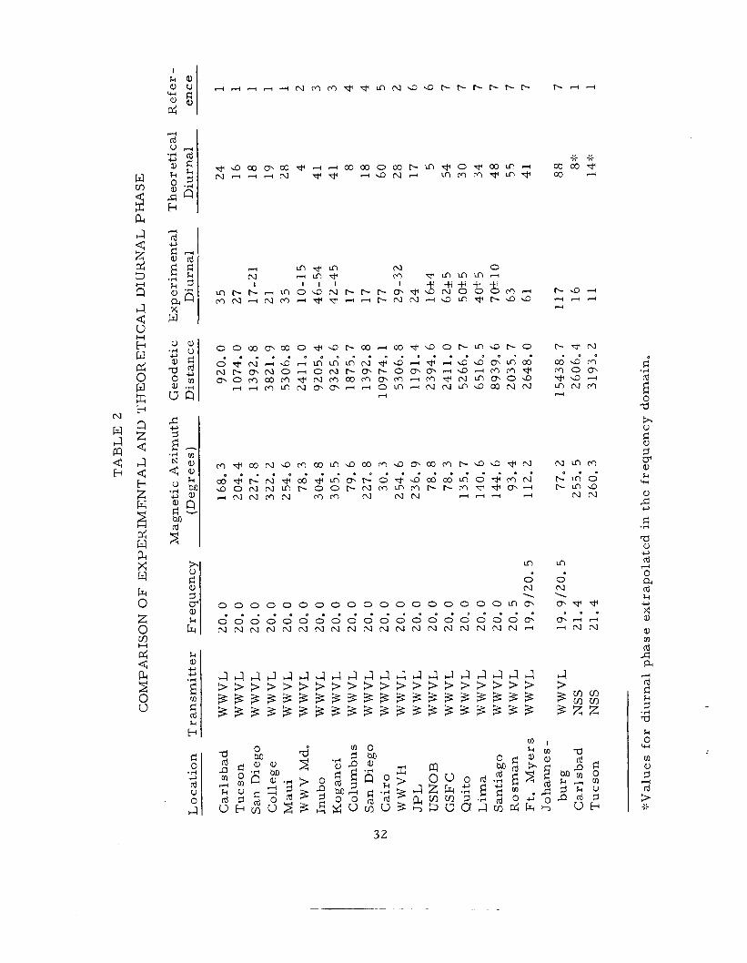
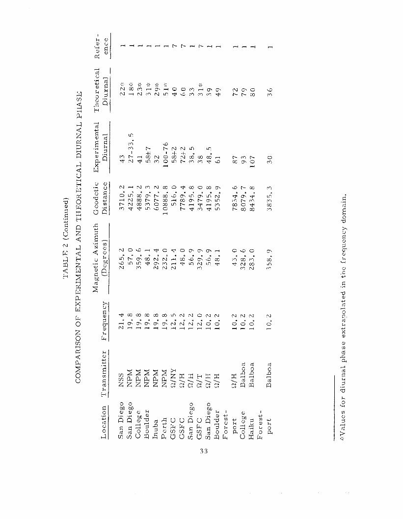
Theoret ical Diurnal Phase . . . . . . . . . . . . 32 Table 2. Comparison of Exper imenta l and
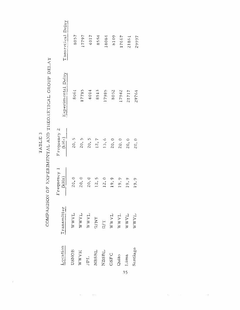
Table 3 . Comparison of Exper imenta l and Theore t ica l Group Delay , . . . . . . . . . . . . 35
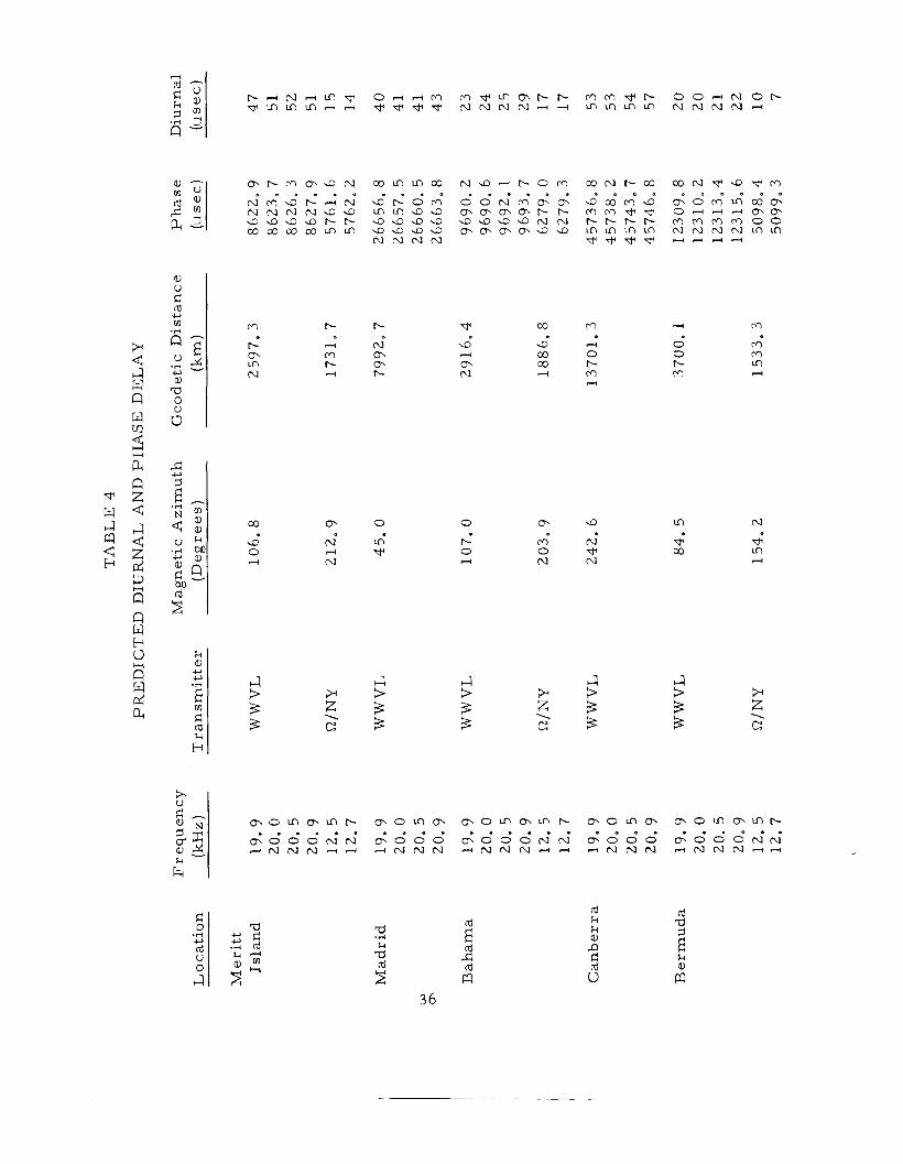
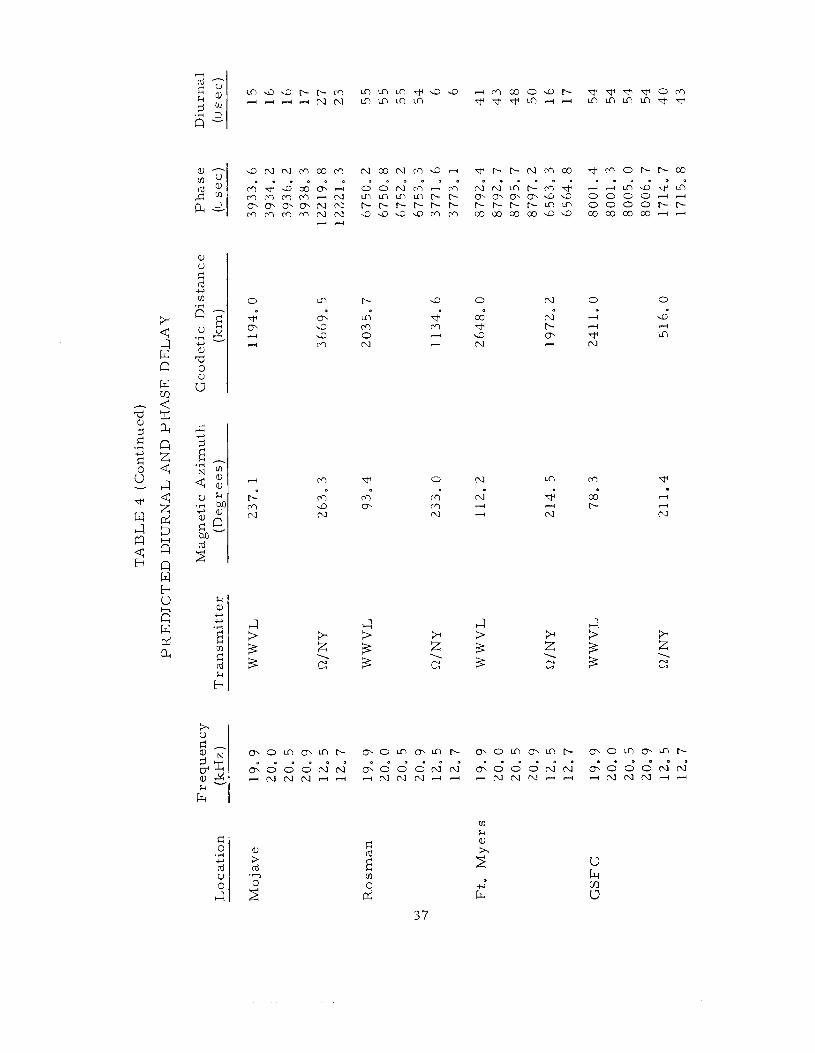
Table 4. Predic ted Diurnal and Phase Delay. . . . . . . . . 36
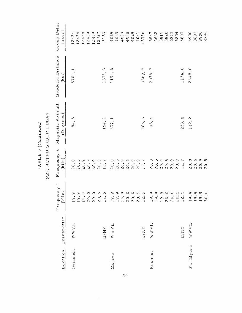
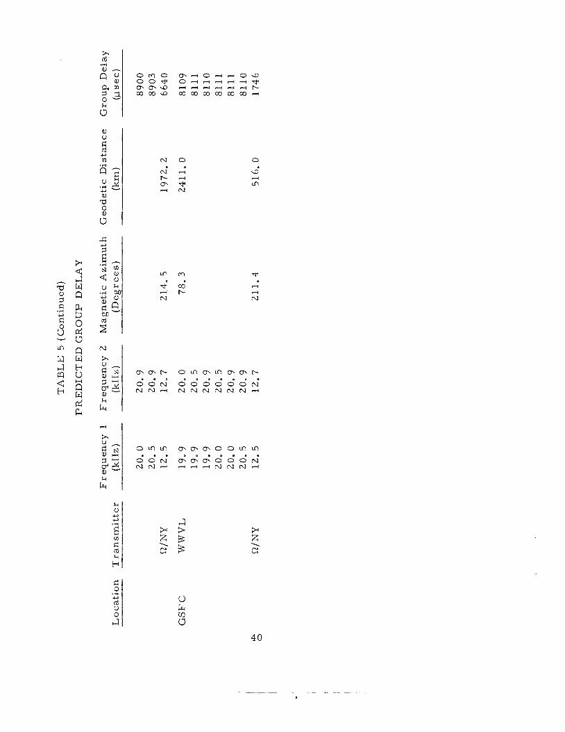
Table 5. Pred ic ted Group Delay . . . . . . . . . . . . . . 38
L i s t of Figures
F igu re 1 . Normal Day Prof i le . . . . . . . . . . . . Figure 2 . Figure 3 .
Normal Night P ro f i l e . . . . . . . . . . . Deeks 1200 Prof i le . . . . . . . . . . . .
Figure 4 . Bain and May Prof i le . . . . . . . . . . . Figure 5 . Diurnal P h a s e . . . . . . . . . . . . . . Figure 6 . Relative Group Delay. Normal Day . . . . . Figure 7 . Normal Night . . . . . . . . . . . . . . Figures 8 . 40: Relative Phase . Normal Day . . . . Figures 41 . 69: Relative Phase. Norma l Night . . . . F i g u r e s 70 . 102: Amplitude. Normal Day . . . . . . F i g u r e s 103 - 128: Amplitude. Normal Night . . . . . Figures 129 - 167: Relative Group Delay. Normal Day . Figures 168 . 204: Relative Group Delay. Norma l Night
F i g u r e s 205 - 233: Diurnal Phase . . . . . . . . . . F i g u r e s 234 . 251: Relative Phase . . . . . . . . . . Figures 252 . 254: Relative Group Delay . . . . . . .
Page
. . . . 41
. . . . 41
. . . . 41
. . . . 41
. . . . 42
. . . . 42
. . . . 43
. . . . 44
. . . . 59
. . . . 74
. . . . 91
. . . . 104
. . . . 124
. . . . 143
. . . . 158
. . . . 165
V
APPLICATION O F VLF THEORY TO TIME DISSEMINATION
W. F. Hamilton and J. L . J e spe r sen
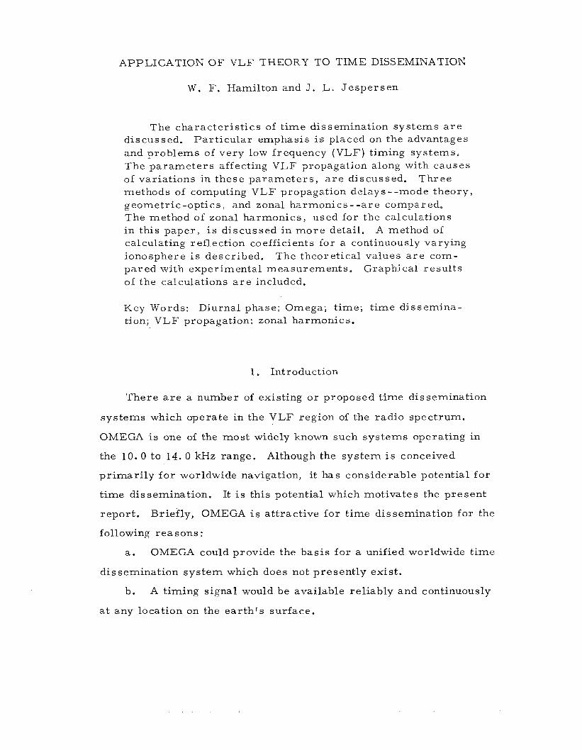
The charac te r i s t ics of t ime dissemination s y s t e m s a r e discussed. Pa r t i cu la r emphasis is placed on the advantages and problems of very low frequency (VLF) timing sys tems. The p a r a m e t e r s affecting VLF propagation along with causes of var ia t ions in these p a r a m e t e r s , a r e discussed. T h r e e methods of computing VLF propagation delays - -mode theory, geometr ic-opt ics , and zonal harmonics - - a r e compared. The method of zonal ha rmon ics , used for the calculations in this pape r , is discussed in m o r e detail. A method of calculating reflection coefficients for a continuously varying ionosphere i s descr ibed. p a r e d with experimental measu remen t s . of the calculations a r e included.
The theoretical values a r e com- Graphical resu l t s
Key Words: Diurnal phase; Omega; t ime; t ime d issemina- tion; VLF propagation; zonal harmonics .
1. Introduction
There a r e a number of existing or proposed t ime dissemination
sys t ems which operate in the V L F region of the radio spectrum.
OMEGA is one of the mos t widely known such sys t ems operating in
the 10 .0 to 14. 0 kHz range.
p r imar i ly fo r worldwide navigation, i t has considerable potential for
t ime dissemination.
report . Briefly, OMEGA i s a t t ract ive for t ime dissemination for the
following reasons :
Although the s y s t e m i s conceived
It is this potential which motivates the present
a . OMEGA could provide the bas i s for a unified worldwide t ime
dissemination s y s t e m which does not present ly exis t .
b. A timing signal would be available reliably and continuously
a t any location on the e a r t h ' s surface.
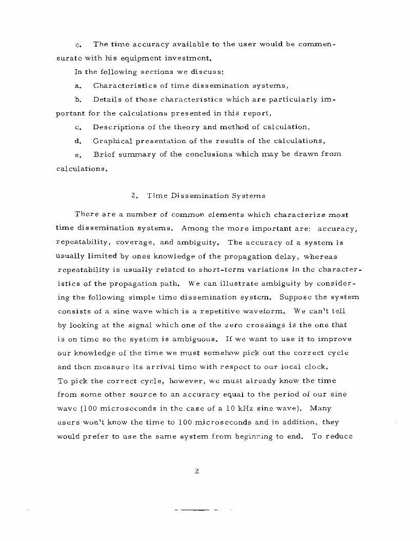
c. The t ime accuracy available to the use r would be commen-
su ra t e with his equipment investment.
In the following sections we discuss:
a.
b.
Charac ter i s t ics of t ime dissemination sys t ems ,
Details of those charac te r i s t ics which a r e par t icular ly im-
portant for the calculations presented in this r epor t ,
c.
d.
e.
calculations
Descriptions of the theory and method of calculation,
Graphical presentat ion of the r e su l t s of the calculations,
Brief summary of the conclusions which may be drawn f r o m
2. T ime Dissemination Sys tems
T h e r e a r e a number of common elements which charac te r ize m o s t
t ime dissemination systems. Among the m o r e important a r e : accuracy ,
repeatabil i ty, coverage, and ambiguity. The accu racy of a s y s t e m is
usually l imited by ones knowledge of the propagation delay, whereas
repeatabil i ty i s usually re la ted to s h o r t - t e r m variat ions in the cha rac t e r -
i s t i c s of the propagation path.
ing the following s imple t ime dissemination system. Suppose the s y s t e m
consis ts of a sine wave which is a repeti t ive waveform. We can't tel l
by looking at the signal which one of the zero c ross ings i s the one that
is on t ime so the sys t em i s ambiguous.
our knowledge of the t ime we mus t somehow pick out the c o r r e c t cycle
and then m e a s u r e i t s a r r i v a l t ime with respec t to our local clock.
To pick the co r rec t cycle, however, we m u s t a l ready know the t i m e
f r o m some other source to an accu racy equal to the period of our sine
wave (100 microseconds in the case of a 10 kHz s ine wave).
u s e r s won't know the t ime to 100 microseconds and in addition, they
would prefer to use the s a m e sys t em f r o m b e g i r i n g to end. - T o reduce
We can i l lus t ra te ambiguity by consider-
If we want to use it to improve
Many
2
the ambiguity i t is usual to t r ansmi t another coherent frequency say at
10 .1 kHz and then inspect the 100 Hz difference frequency.
out the on- t ime cycle of the 100 Hz difference frequency, we need
only know the t ime to 1 0 mill iseconds (the period of a 100 Hz s ine wave).
We s e e that by adding m o r e signals a t different f requencies , we can
reduce the ambiguity of the sys t em to any des i r ed level. However, a s
we reduce the ambiguity, we mus t at the s a m e t ime inc rease the amount
of frequency spec t rum which the sys t em occupies. For very low f r e -
quency sys t ems , we can’t very well put on modulations which requi re
l a r g e bandwidths.
on a 10 kHz c a r r i e r .
be increased by averaging many measu remen t s .
To pick
That i s , you can’t put a signal which occupies 50 kHz
In many cases , the usefulness of the s y s t e m may
3. P a t h Delay
P a t h delay predictions, and thus, the accu racy of the s y s t e m a r e
l imited by knowledge of the geometry of the t r ansmi t t e r and use r loca-
tions and by the availability of information concerning the propagation
medium. At V L F , a t g rea t distances f r o m the t r ansmi t t e r , the signal
velocity has a near ly constant value, whereas near the t ransmi t te r the
average velocity between the u s e r and the t ransmi t te r changes in a n
i r r egu la r way a s a function of distance.
regular to i r r egu la r occurs a t a distance of about 10, 000 ki lometers
f r o m the t ransmi t te r .
in te res t .
signal-to-noise ra t io i s g rea tes t and r ece ive r s ’ costs , in principle,
should be a t a minimum.
path delay, we mus t introduce the ideas of phase velocity, V and
group velocity, V a s they apply to V L F .
In general , the t ransi t ion f r o m
In this repor t , the i r r egu la r region i s of m o s t
It i s important to consider this near region because h e r e the
To consider i n m o r e detail the p rob lem of
P’
g’
3

Let us consider a s imple two-frequency timing system. Suppose
we have two closely spaced cw signals at f requencies f l and f 2 where
f2 - f l = A f ,
t ime m a r k e r to identify a specific cycle of e i ther c a r r i e r frequency.
This removes ambiguities and a m o r e p rec i se t ime of a r r i v a l m e a s u r e -
ment i s made at the higher c a r r i e r frequency.
quency signal will t r ave l f r o m t r ansmi t t e r to rece iver with a group
velocity which depends upon the phase velocity v e r s u s frequency cha r -
ac t e r i s t i c of the propagation medium, Specifically, the group velocity
is related to phase velocity V
In this sys tem, the beat frequency Af i s used a s a coa r se
The difference f r e -
by the following expression: P
where u) is the angular frequency.
velocity breaks down i f the derivative - ( w / V ) i s not well behaved,
In a d ispers ive medium, such a s we a r e considering a t V L F , Vp is a
function of w so that the group delay, t over a path r is given by the
following expression:
We s e e that the concept o f group d
dw P
d
At very low frequencies the phase velocity ve r sus frequency dependence
cannot be expressed a s a s imple function of the proper t ies of the propa-
gation medium, except perhaps a t g rea t dis tances f r o m the t ransmi t te r .
The m o s t accura te r e su l t s a r e obtained f r o m numer ica l solutions of
Maxwell 's equations, i. e. , full wave solutions, with some rea l i s t i c
model of the ionosphere, the approach taken in this paper .
difference frequency may t ravel with a group velocity that i s different
than the phase velocity of e i ther one of the two c a r r i e r f requencies , the
Since the
4
difference frequency signal may slip in phase with respec t to e i ther one
of the c a r r i e r frequencies a s a function of distance f r o m the t ransmi t te r .
This could lead to incor rec t cycle identification of the c a r r i e r frequency
unless the difference in velocit ies i s known.
can cor rec t ly identify a cycle by using different group and phase
velocit ies. Unfortunately, the concept of group velocity applies only
a t g rea t distances f r o m the t ransmi t te r , where the phase velocity
ve r sus frequency charac te r i s t ics a r e well behaved,
- ( , / V ) i s well behaved. Near the t r ansmi t t e r , a different approach
mus t be used.
we will consider f i r s t how a V L F pulse would propagate in this region.
At grea t distances, one
i. e . ,
d d? P
To help i l lus t ra te what i s happening near the t r ansmi t t e r
T h e r e a r e two distinct effects which one mus t consider. F i r s t ,
the average propagation velocity of the pulse (group velocity) may be
equal to o r l e s s than the velocity of light, Second, the. pulse may be
changing i t s shape a s i t propagates through the medium.
point on the pulse has been tagged a s the t ime re ference point, a t the
t r ansmi t t e r , i t i s necessa ry to de te rmine how this "tag" point is mapped
into i t s new position a s the pulse d is tor t s during i t s propagation away
f r o m the t ransmi t te r . If this i s not known, i t wi l l not be c lear to the
use r which point on the received pulse r ep resen t s the re ference point
a s t ransmit ted, In addition, having cor rec t ly identified the tagged
point, one mus t a lso consider the fact that the average pulse velocity
may be l e s s than the velocity of light, A multifrequency V L F sys t em
is somewhat s imi la r to the propagation of a pulse in the following sense:
A short pulse of length r consis ts of a spec t rum of f requencies , i. e . ,
a number of Four ie r components which occupy a spectral region approx-
imately equal to l / - g In a d ispers ive medium, such a s the ionosphere,
each one of these Four ie r components wi l l t rave l with a different phase
velocity.
If a par t icular
In a sense then, when w e use a VLF tone sys tem, we a r e
5
sending one Four i e r component a t a t ime and the u s e r , i f he des i r ed ,
could by storing the received tones add them together to produce some-
thing looking l ike a pulse.
well defined shape a s i t left the t ransmi t te r .
p roper t ies of the propagation medium this composi te waveform wi l l
change i t s shape a s a function of dis tance f r o m the t r ansmi t t e r until
i t has propagated out to the region where the phase velocity is well
behaved. Beyond this point, the composi te waveform would maintain
essent ia l ly the s a m e shape a s a function of dis tance although i t would
not be the s a m e a s t ransmit ted.
t r a n s f e r r a l , i t is n e c e s s a r y to know in detail the s t ruc tu re of this
composi te waveform as a function of distance f r o m the t ransmi t te r .
This composi te waveform would have some
Because of the d ispers ive
To use the t ime sys t em for accura te
Similar ly , u se of the V L F multitone s y s t e m for accura te t ime t r a n s -
f e r r a l r equ i r e s detailed knowledge of the phase ve r sus frequency and
dis tance charac te r i s t ics of the signals. We wi l l t u rn to the detai ls of
theoret ical calculations of V L F phase velocity in Sections 4 and 5.
4. Important P a r a m e t e r s for V L F Calculations
The phase velocity v e r s u s frequency charac te r i s t ics a t VLF a r e
par t icular ly sensit ive to the propagation medium.
medium is charac te r ized by the conductivity of the ground, the e lec t r ica l
p roper t ies of the ionosphere,the direction of propagation w i t h respec t to
the ea r th ' s magnet ic field,and the s t rength of the magnet ic field,
The propagation
The mos t important e lec t r ica l p roper t ies of the ionosphere for
V L F calculations a r e :
a.
b.
C.
The electron density v s height.
The proton density v s height.
The collision frequency between charged and neutral par t ic les
v s height.
6
The composition of the ionosphere is not static. Many different
types of events, for example solar f l a r e s , can cause sho r t - t e rm
variat ions in the ionization.
do not take these sho r t - t e rm variat ions into account but a r e based on
the average proper t ies of the ionosphere a s i t might appear a t noon and
at midnight of the s u m m e r sols t ice a t midlatitudes.
The theoret ical calculations in this repor t
T h e r e i s considerable experimental evidence that the propagation
delay of a VLF signal f r o m one day to the next a t the s a m e t ime of day
is repeti t ive to a few microseconds,
p roper t ies of the ionosphere should be sufficient for many applications.
This i s an at t ract ive feature of VLF signals for t ime dissemination.
We l i s t he re briefly some physical p rocesses responsible for these
average proper t ies .
s o that consideration of the average
The mos t important fac tors a r e a s follows:
a. Solar X - r a y s (2 10 A ) above 85 k m a t sunspot minimum and
above 70 k m a t sunspot maximum;
b,
range;
c .
The ionization of NO by solar Lyman -a in the 70 to 90 k m
P r i m a r y cosmic r ays below 70 k m with the flux increasing by
a factor of about 4 f r o m sunspot maximum to minimum.
subject is very volatile and recent work indicates that water vapor
and metastable s ta tes of O 2 a r e important.
However, this
d e Various react ions between f r ee electrons, ions and neutral
par t ic les ; and
e Mechanical and electrodynamical forces which redis t r ibute
the ionization.
Although, a s s ta ted previously, the calculations in this repor t a r e
based upon the average proper t ies of the ionosphere, i t is important to
rea l ize that t he re a r e sho r t - t e rm variat ions in the medium.
t e r m phase variations a r e one of the mos t noticeable features of a VLF
The shor t -
7
record.
u tes ) than one would expect f r o m so lar controlled phenomena and a r e
undoubtedly a t t imes related to the motions in the neutral a tmosphere .
These fluctuations a r e much shor te r (of the o r d e r of 30 min -
T h e r e is not much information on the turbulent s t ruc tu re of the
mesosphe re (the region of the neutral a tmosphe re which overlaps the
D Region) because this is a region that i s too high for balloon soundings
and too low for satell i tes.
i r r egu la r s t ruc tu re in this region based upon rocket and me teo r t r a i l
investigations. F o r example, sodium cloud m e a s u r e m e n t s by Blamont
and Jage r
they explained by a combination of turbulent mixing and molecular
diffusion. About 10 y e a r s ago, Greenhow and Neufeld suggested the
p re sence of l a r g e sca le i r r egu la r i t i e s in the 80 -90 k m region based
upon r ada r observations of me teo r t r a i l s . However, t h e r e i s some
controversy about these observations s ince l a t e r measu remen t s by
Manring, et a l . , via rocket sodium cloud measu remen t s suggested
that the turbulence explanation may be spurious and in fact may be due
to the rocket.
and Drazin
propagation of gravity waves into the upper a tmosphere .
However, t he re i s some information on the
1 . indicated the existence of i r r egu la r i t i e s below 100 k m which
2
3
An al ternat ive explanation has been made by Charney
who suggest that the i r r egu la r i t i e s a r e produced by the 4
In any case , phase fluctuations of VLF signals a r e in some fashion
related to the i r r egu la r s t ruc tu re of the mesosphere .
A s discussed e a r l i e r , rea l i s t ic calculations of V L F radio fields a r e
obtained f r o m full wave solutions and for the present these solutions
have only been obtained for plane s t ra t i f ied ionospheric models.
the possibility of using this approach to obtain wavefields for a m o r e
complicated i r r egu la r ionosphere does not s e e m part icular ly pract ical
a t the present t ime and i t appears n e c e s s a r y to r e s o r t to s impler m o r e
approximate methods.
Thus,
8
A s an example of one such possible approach, suppose that one is
s e v e r a l thousand k i lometers f rom a V L F t ransmi t te r .
the phase velocity of the radio signal i s near ly constant ( this cor responds
to the situation in a waveguide where mode 1 i s dominant) and i s given
approximately by
At such a dis tance,
where ) is the radio wavelength, h
l a y e r , and c the velocity of light. To a f i rs t approximation, we might
consider that the effect of a l a r g e i r r egu la r i ty would be to change the
height of the reflecting layer by a n amount 1 h, which would in t u r n
the height of the ionospheric reflecting 0
a l t e r the phase velocity. Thus f rom the equation above, we obtain 2
i;n - -- v 16h h
P 0 0
since < < h . 0
This change in phase velocity would produce a change i n the phase
of tl-e received signal which could be interpreted in a s t ra ight forward
manner for th i s situation. However, the situation becomes m o r e
complicated when the i r r egu la r i t i e s a r e small compared to the path
length o r to the radio wave length.
p roblem theoretically.
developed specifically for V H F forward sca t t e r problems and has
attempted to adapt i t f o r the interpretation of V L F phase measurements .
Although th is work appears to be far f r o m exact, it does give s o m e
interest ing resu l t s , Specifically, Crombie considers the two cases
when V L F phase measu remen t s a r e made on a distant t r ansmi t t e r using
two V L F receiving sites.
receiving s i t e s a r e in l ine with the t r a n s m i t t e r , and in the second case
( t r a n s v e r s e c a s e ) occur s when the l ine joining the two r ece ive r s is
5 Crombie has attempted th i s
6 He has taken the work by Rice which was
In the f i r s t ca se (longitudinal c a s e ) the two
9
perpendicular to the l ine between one of the r e c e i v e r s and the t r ansmi t t e r .
He then takes s o m e experimental data of Harg reaves which apply to the
t r a n s v e r s e c a s e and concludes that the ave rage s i ze of the i r r e g u l a r i t i e s
is about 65 k m and that the horizontal dr i f t velocity i s about 35 m / s e c .
Crombie compares these values with some r e s u l t s f r o m Hines , (which
appear to apply to the region in question) which predic t a horizontal
velocity of about 100 m / s e c . for internal gravi ty waves with horizontal
components o f 6 5 km. Although the predicted value i s higher than that
deduced by Crombie, the values a g r e e within a n o r d e r of magnitude.
7
8
5. Theory of Calculations
T h r e e approaches to theore t ica l V L F calculations have seen wide 9 usage: (1) Wave guide mode theory, (2) geomet r i c opt ics , and ( 3 ) zonal
harmonics .
one mode need normal ly be considered.
t r a n s m i t t e r and r ece ive r d e c r e a s e s , m o r e modes a r e necessa ry . Some
disadvantages a r e that physical in te rpre ta t ion of modes is difficult and
the introduction of varying propagation p a r a m e t e r s along the path
becomes ve ry complicated. It i s possible that significant modes may
be overlooked. In addition, un less a F o u r i e r t r a n s f o r m into the t i m e
domain i s employed, mode theory does not account for the observed
difference in a r r i v a l t i m e between the ground wave and the var ious
sky waves
Mode theory has the advantage that a t l a r g e d is tances only
A s the dis tance between the
Geometr ic op t ics , on the other hand, lends i tself well to c l ea r
physical interpretat ion.
wave.
m i t t e r , jus t the opposite of mode theory,
th i s theory become m o r e valid with increas ing frequency, but a r e in
genera l not valid a t V L F except ve ry nea r the t r ansmi t t e r .
Various "hops" a r r i v e l a t e r than the ground
The accu rac i e s of geometr ic opt ics a r e g rea t e s t n e a r the t r a n s -
The approximations m a d e by
Geometr ic
10
optics i s not a r igorous theory f o r electromagnetic wave propagation in
the V L F region.
The mathematical derivation of the zonal harmonic and geometr ic
s e r i e s representat ions f o r electromagnetic wave propagation i s well
documented by Johler
be pr imar i ly nonmathematical i n an attempt to give physical insight to
this method.
10, 11, 12, 13, 14, 15 The approach used h e r e wil l
The use of zonal harmonics in propagation formulae was introduced 16
ear ly in the 20th century by Debye
L o r d Rayleigh
p rac t i ca l application of this theory could be accomplished.
speed digital computer allows summation of the l a r g e number of t e r m s
that a r e requi red for convergence of the s e r i e s . (Here convergence is
used to mean that additional t e r m s do not significantly effect the resu l t . )
In addition, new theoretical advances have great ly reduced the number
of t e r m s required for convergence.
( for electromagnetic waves) and 17
( for sound). It was not, however, until recently that
The high
Zonal harmonics allow the introduction of r igorous analysis while
maintaining the c l ea r physical interpretat ion of geometr ic optics, The
t e r m in the classical zonal harmonic s e r i e s containing both the ground
and ionospheric reflection coefficients can be represented as a geo-
m e t r i c s e r i e s ,
harmonic s e r i e s before the geometr ic se r ies - -y ie lds a s e r i e s , each
t e r m of which i s analogous to the geometr ic optic s e r i e s .
o r d e r t e r m of the geometr ic s e r i e s is the ground wave and the jth term
rep resen t s a wave which has suffered j reflections f r o m t h e ionosphere.
Inverting the o r d e r of summation--summing the zonal
The zero th -
-
The l a r g e number of t e r m s ordinar i ly required for convergence of
the zonal harmonic s e r i e s i s found to be necessa ry only because the
ground wave i s included i n the calculations.
converge with approximately one-fifteenth the number of t e r m s ,
the ground wave may be computed m o r e effectively by other means ,
the remaining t e r m s of the geometr ic s e r i e s can be rapidly computed,
The higher o r d e r t e r m s
Since 18
11
Very few t e r m s a r e required for convergence of the geometr ic
s e r i e s a t VLF. Under no rma l conditions, 10 t e r m s (i. e . , hops) have
been found sufficient for convergence to distances of 8 , 000 to 10 , 000
ki lometers . Grea ter dis tances may requi re a few m o r e t e r m s .
Each t e r m of the geometr ic s e r i e s may be thought of a s a se t of
‘In-waves” (the n t e r m s of the zonal harmonic s e r i e s ) .
waves i s incident on the ionosphere and the ground a t an angle which i s
an approximate function of n.
of incidence which a r e given exactly by functions of n.
has been noticed between using r e a l and complex angles of incidence since
normal ly the imaginary portion i s quite small . )
determining factor for the number of t e r m s required for convergence.
The s e r i e s converges abruptly a s the angle of incidence approaches
9 0 degrees . The contribution of t e r m s where the angle of incidence
is l e s s than approximately 30 degrees is negligible.
even fewer t e r m s a r e required.
Each of the n-
(The r igorous theory uses complex angles
Li t t le difference
This function of n i s the
Consequently,
Because of l a t e ra l displacement a t both the ionosphere and the
ground, no specific angle of incidence is required for a wave to reach
a par t icular distance. La te ra l displacement a s used h e r e means that
a wave may be t rapped and propagate radially within the ionosphere or
ground for some distance before emerging again to continue no rma l
propagation ( s e e figs. 1 2 through 15, pp. 45-48, Johler and Mellecker ,
1970--Ref. 15). Most of the reflection does, however, take place near
the angle predicted by geometr ic optics.
Each n-wave contains a factor which may be called the effective
reflection coefficient.
reflection coefficients for ordinary and extraordinary reflection f r o m
the ground and ionosphere.
tion of both the t r ansmi t t e r and rece iver antennae, for example, only
In essence this factor i s the sum of a l l possible
F o r the case of ver t ica l e lec t r ic polar iza-
12
ordinary reflection can effect the field fo r the f i r s t hop so the effective
reflection coefficient i s T Both ordinary and extraordinary r eflec-
tion can affect the second hop field and the effective coefficient is eeo
T R T t T R T Higher o rde r coefficients become very e m m m e ee e ee
complicated.
with the f i r s t subscr ipt denoting the incident polarization and the second
the reflected polarization ( e i s ver t ical e lec t r ic and m i s ver t ical mag-
netic). The ground reflection coefficient, R , needs only one subscr ipt
since no abnormal component i s generated during ground reflections.
Here T stands fo r the ionospheric reflection coefficient
Since mos t of the reflection for a given "hop" takes place within
a region, local reflection coefficients may be introduced. Fo r example,
a land sea boundary changes the reflection coefficient of the ground and
may be incorporated. Similar ly , i f par t of the path is in sunlight while
the r e s t is in darkness ( io e . , the " terminator" occur s along the propa-
gation path) this fact may be used in the analysis .
The ionospheric reflection coefficients which a r e mos t readily
These may be used a s an available a r e plane F r e s n e l coefficients.
approximation to the t r u e coefficients.
quite good if the coefficients a r e multiplied by a convergence-divergence
factor . The best method, however, i s to allow complex angles of
incidence.
imaginary t e r m will normally be smal l , but i t may not be mathematically
negligible.
The approximation becomes
It has been s ta ted ea r l i e r that the contribution of the
Since the only distance related portion of each n-wave i s the
Legendre function, the field a t many dis tances can be calculated s imul-
taneously.
min imal i nc rease in computation t ime.
Upwards of 2 0 0 distances may be calculated with only
It i s n e c e s s a r y to compute the reflection coefficients for each n.
This i s no difficulty for the ground reflections since this calculation
13
is relatively s t ra ightforward and does not consume much computer
t ime. The ionospheric reflection coefficients, however, a r e compu-
tationally quite complicated and can consume a s much a s 2 minutes
of computer t ime for each set of coefficients required.
reflection coefficients a r e a smooth function of angle of incidence
(of n ) , i t is pract ical to s e t up a table of reflection coefficients and to
interpolate on this table to obtain the des i r ed coefficient.
should be made in such a way that no extrapolation is necessary .
Because the
The table
The e lec t r ica l quali t ies of the ionosphere may be character ized
by electron and ion density prof i les , and a collision frequency model.
To facil i tate calculation of the reflection coefficients, the ionosphere
is divided into layers .
By increasing the number of l a y e r s , th i s representat ion can be made
a s c lose a s des i red to the continuous distribution.
Each layer i s a s sumed to have uniform densit ies.
Maxwell 's equations and the equation of motion of the electron a r e
solved yielding t ransmi t ted and ref lected portions of the incident wave
f o r each of the layers .
waves and solving for continuity a t the boundaries between each of the
l a y e r s , the ref lect ion coefficients a r e obtained.
By keeping t rack of these upgoing and downgoing
Coupling of the ver t ica l e lec t r ic and ver t ical magnet ic polar iza-
tions within the ionosphere causes the generation of an abnormal com-
ponent and necess i ta tes calculation of two reflection coefficients for
the ver t ica l e lec t r ic incident polarization, Also, since ground ref lec-
t ions do not change the polarization of the incident wave ( io e. , t he re i s
no coupling at the ground) , i t i s n e c e s s a r y to compute reflection
coefficients fo r no rma l and abnormal ionospheric reflection of ver t ica l
magnet ic incident polarization. To s u m m a r i z e , four reflection coeffi - cients mus t be computed fo r each angle of incidence; (1 ) ver t ica l e lec t r ic
polarization of the incident and ref lected wave ( T ) , ( 2 ) ver t ica l e lec t r ic ee
14
polarization of the incident wave with abnormal o r ve r t i ca l magnetic
polarization of the reflected wave ( T ) , ( 3 ) ve r t i ca l magnetic polar iza-
tion of the incident and reflected wave ( T ), and (4 ) ve r t i ca l magnetic
polarization of the incident wave and ve r t i ca l e lec t r ic polarization of the
reflected wave ( T ).
e m
mm
m e NOTE: Vert ical e l ec t r i c polarization is in quadra ture (a t 9 0 degrees )
to ver t ical magnetic polarization and may also be called horizontal mag-
netic polarization, Similar ly , ve r t i ca l magnetic polarization may be
called horizontal e l ec t r i c polarization.
Each reflection coefficient gives the phase and amplitude of the
ref lected wave.
ionosphere.
Interpolation on th i s wildly varying phase can be ve ry inaccurate.
p roblem is solved by re - re ferenc ing the phase to a height where the
phase i s slowly varying with angle of incidence.
t imes r e f e r r e d to as the effective reflection height.
The phase i s normally re ferenced to the bottom of the
This causes the phase to va ry rapidly with angle of incidence.
The
This height i s some-
6. The Calculations
Table 1 lists the calculations that a r e repor ted i n this paper.
Throughout these calculations a magnetic dip of 70 degrees and a mag-
netic f ie ld s t rength of 4 0 ampere - tu rns /me te r have been employed.
These values a r e a good approximation of the magnetic field vector
experienced in the United States,
graphs a r e re la t ive to a medium where the index of refract ion is 1, 0001,
All of the phase and group delay
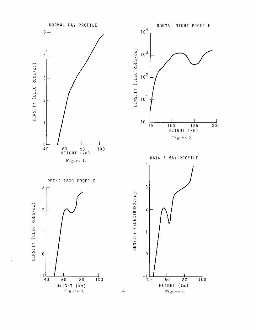
Two ionospheric prof i les (electron density a s a function of height
above the surface of the e a r t h ) designated normal day (fig. 1 ) and
normal night (fig. 2 ) , have been used f o r the majori ty of the calculations
with s ix other prof i les used to demonstrate the types of fluctuations one
might expect under ce r t a in conditions.
night prof i les were r a i sed and lowered 2. 5 km.
The no rma l day and normal
While this i s admittedly
15
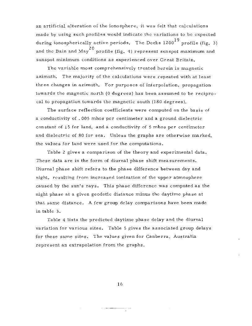
an ar t i f ic ia l a l terat ion of the ionosphere, i t was felt that calculations
made by using such prof i les would indicate the var ia t ions to be expected
during ionospherically active periods. The Deeks 1200 profile (fig. 3 )
and the Bain and May
sunspot minimum conditions a s experienced over Grea t Britain.
19
2 0 prof i le (fig. 4 ) r ep resen t sunspot maximum and
The var iable mos t comprehensively t rea ted herein i s magnet ic
azimuth. The majori ty of the calculations w e r e repeated with a t l ea s t
t h ree changes in azimuth. F o r purposes of interpolation, propagation
towards the magnet ic nor th ( 0 deg rees ) has been a s sumed to be rec ipro-
cal to propagation towards the magnet ic south (180 degrees ) .
The surface reflection coefficients were computed on the bas i s of
a conductivity of . 005 mhos p e r cent imeter and a ground dielectr ic
constant of 1 5 for land, and a conductivity of 5 mhos p e r cent imeter
and dielectr ic of 80 for sea .
the values for land were used for the computations.
Unless the graphs a r e otherwise marked ,
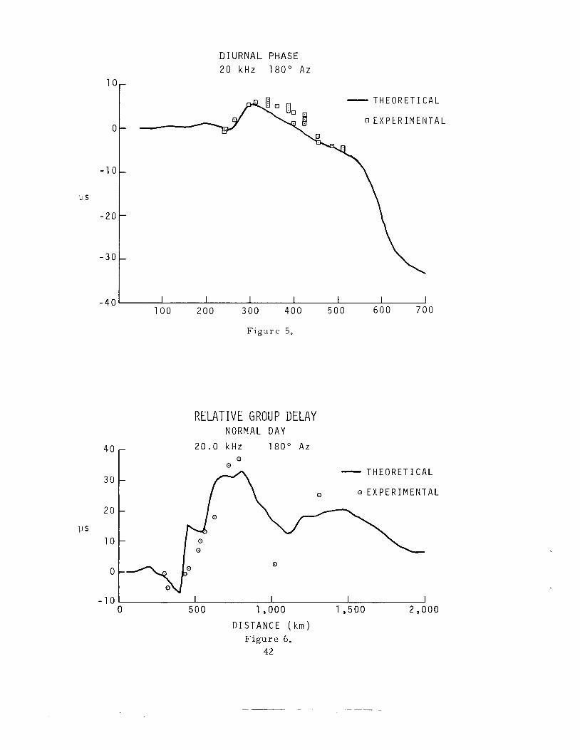
Table 2 gives a compar ison of the theory and experimental data.
These data a r e in the f o r m of diurnal phase shift measu remen t s .
Diurnal phase shift r e f e r s to the phase difference between day and
night, result ing f r o m increased ionization of the upper a tmosphe re
caused by the sun 's rays .
night phase a t a given geodetic distance minus the daytime phase a t
that s a m e distance.
in table 3 .
This phase difference was computed a s the
A few group delay compar isons have been made
Table 4 l i s t s the predicted daytime phase delay and the diurnal
var ia t ion for var ious s i tes .
f o r these s a m e s i tes . The values given for Canberra , Austral ia
r ep resen t a n extrapolation f r o m the graphs.
Table 5 gives the assoc ia ted group delays
1 6
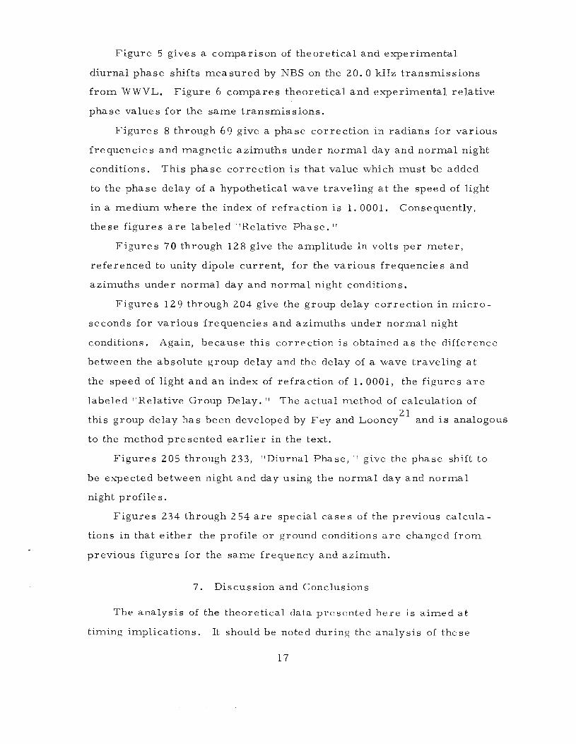
Figure 5 gives a comparison of theoret ical and exper imenta l
diurnal phase shifts measu red by NBS on the 2 0 . 0 kHz t r ansmiss ions
f r o m WWVL.
phase values fo r the same t ransmiss ions .
F igure 6 compares theoret ical and exper imenta l re la t ive
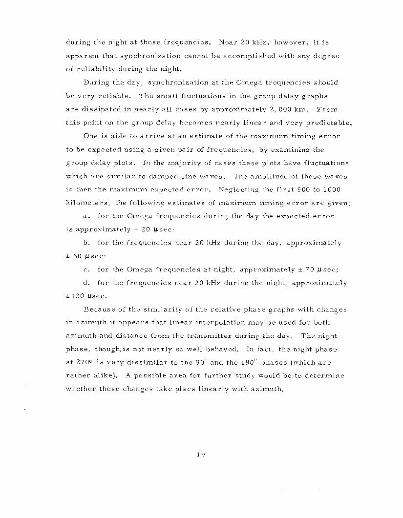
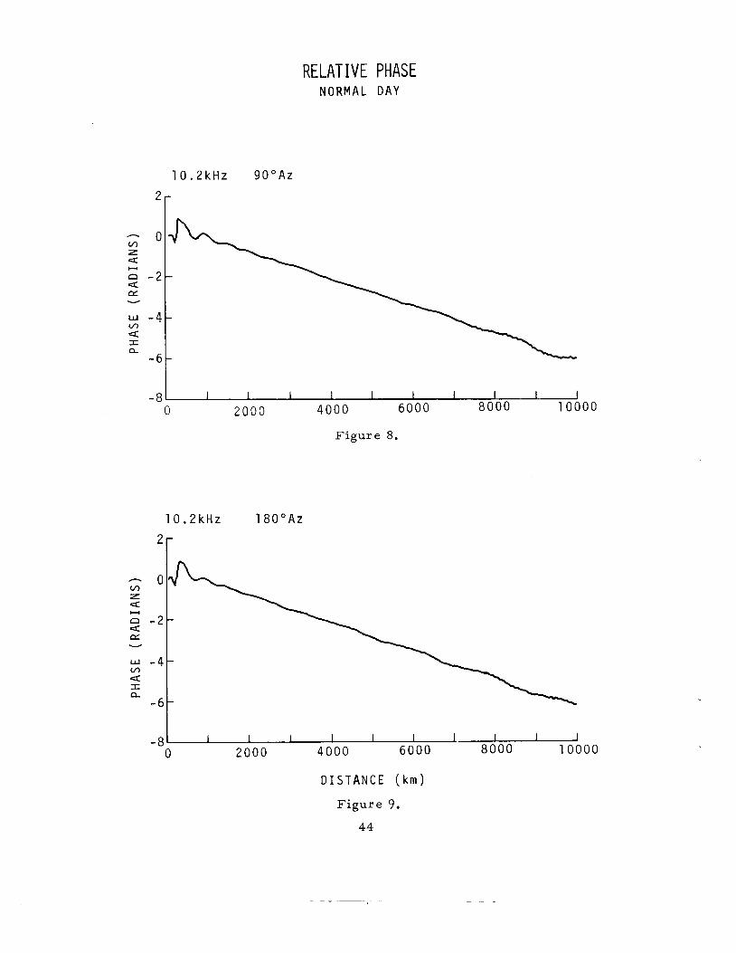
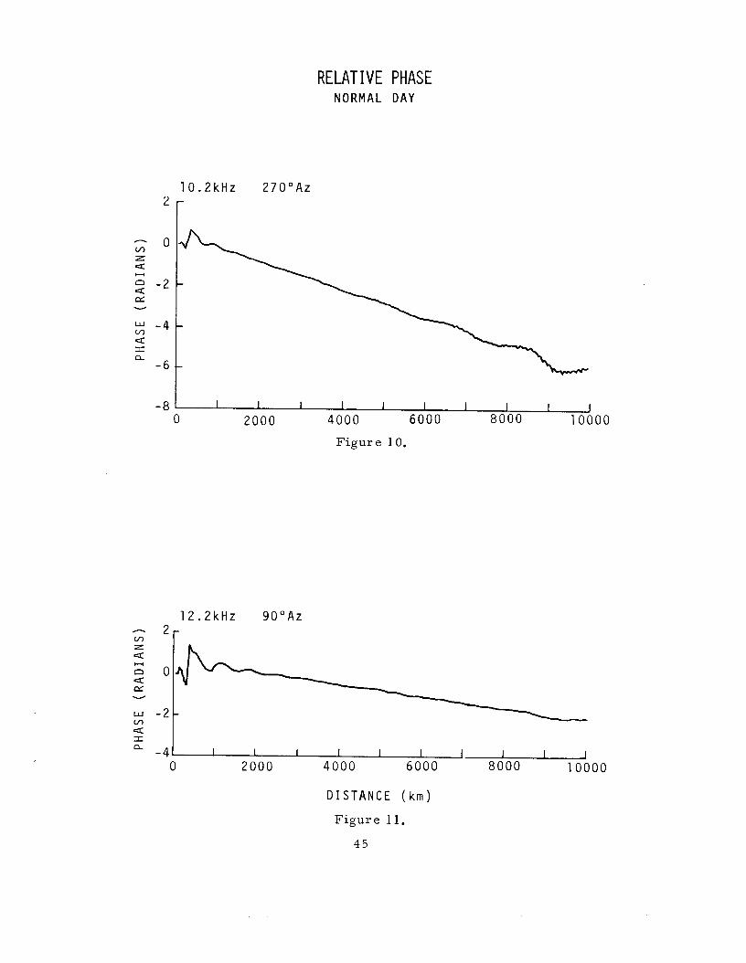
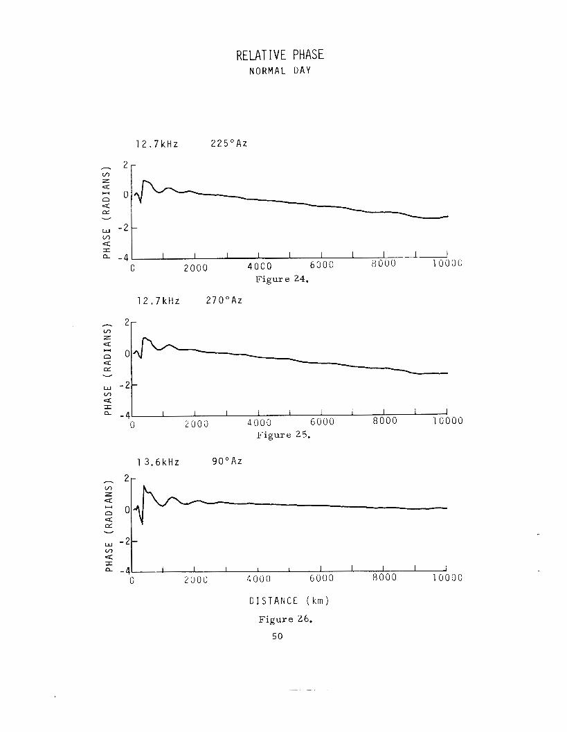
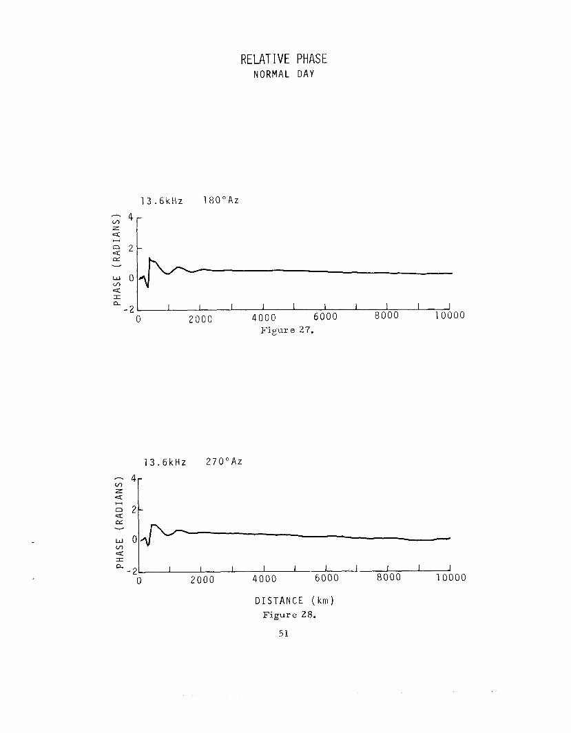
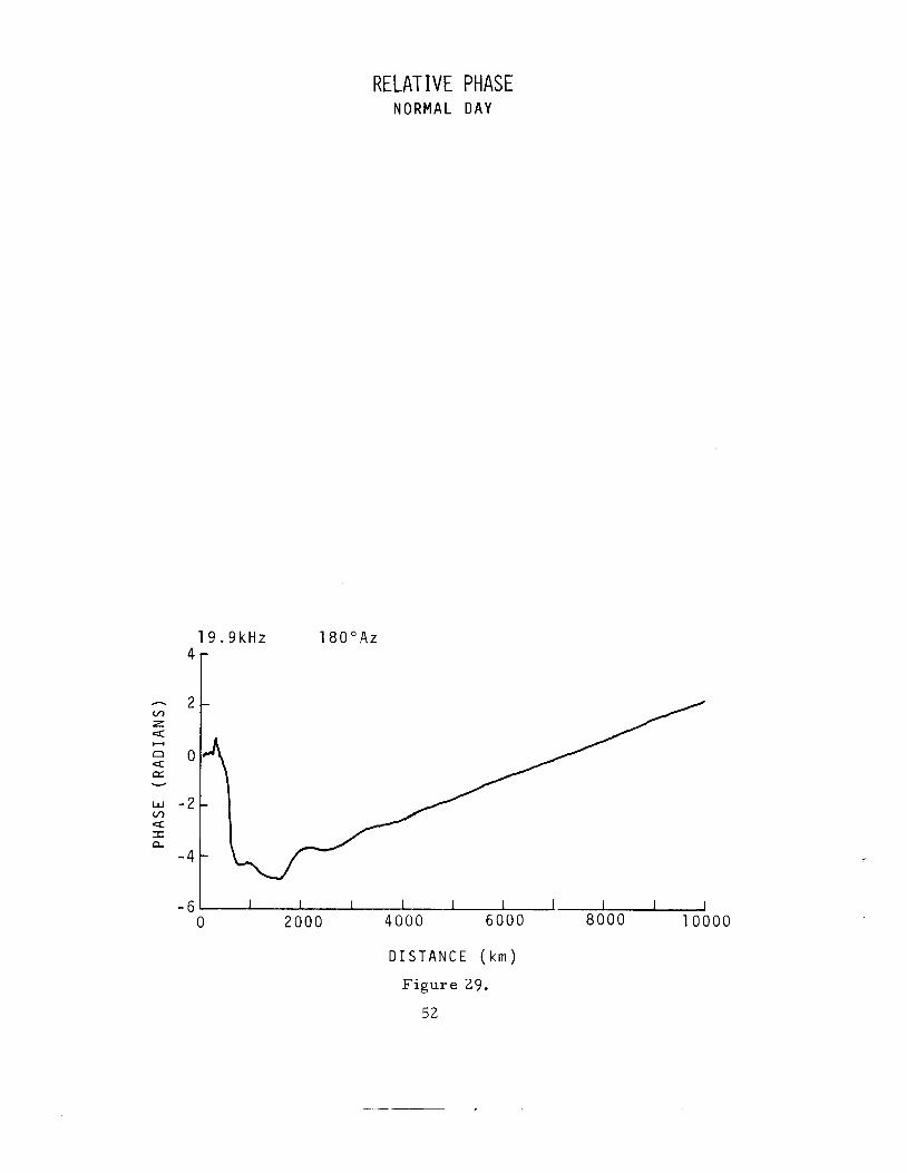
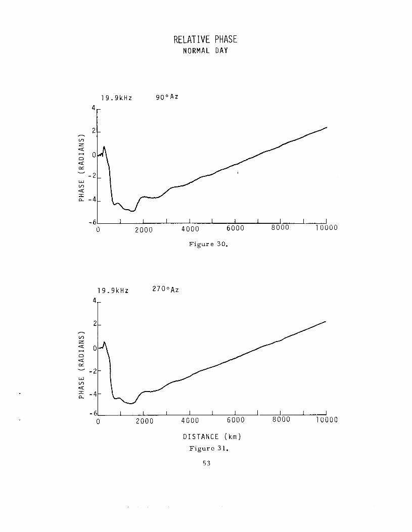
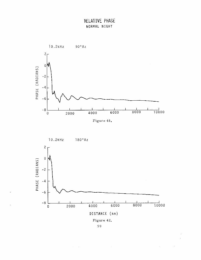
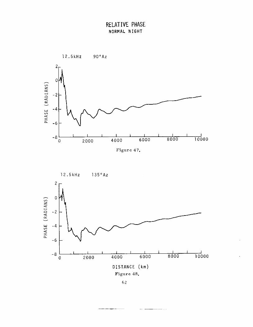
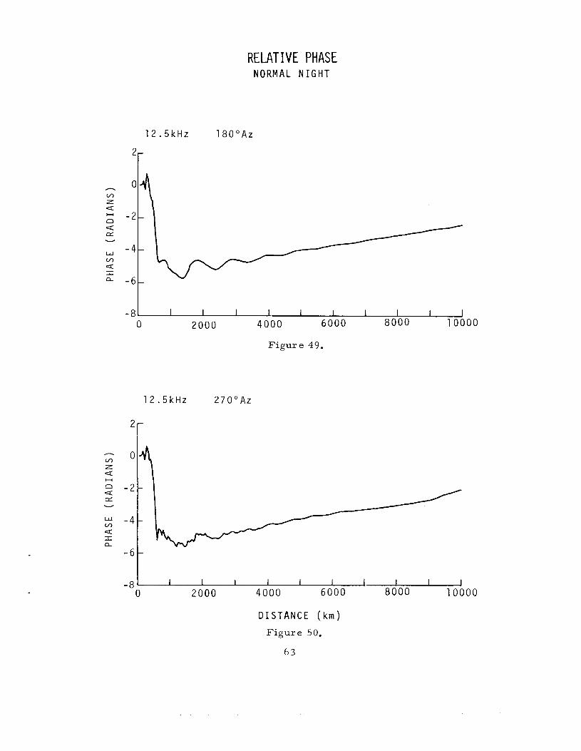
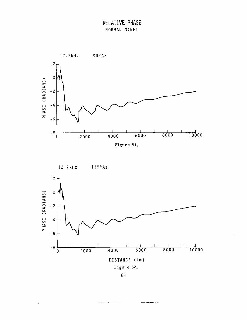
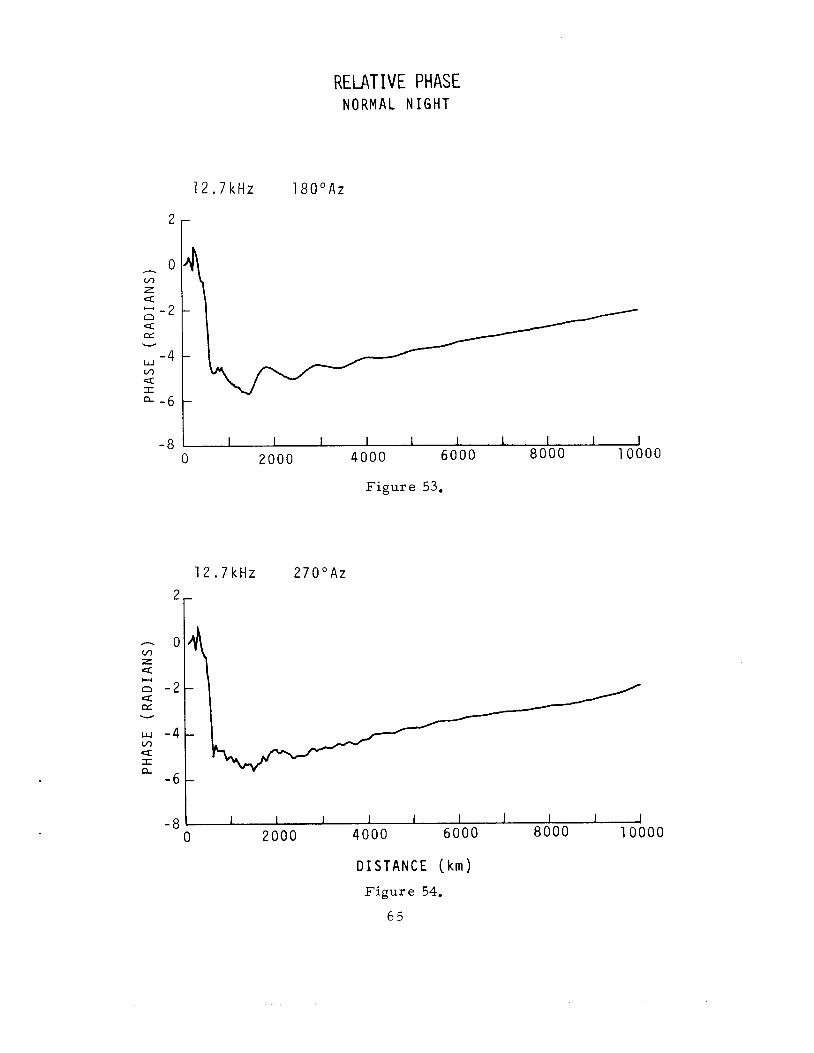
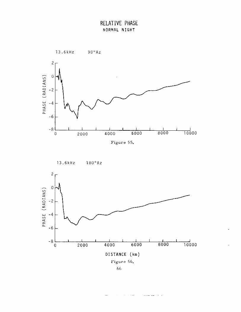
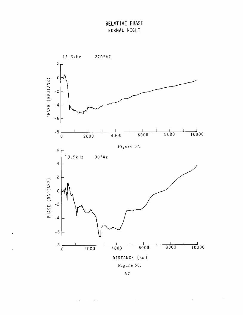
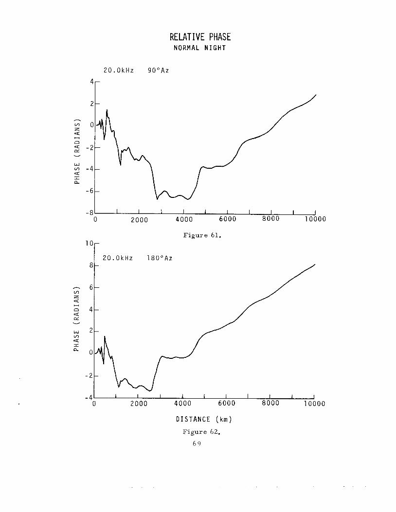
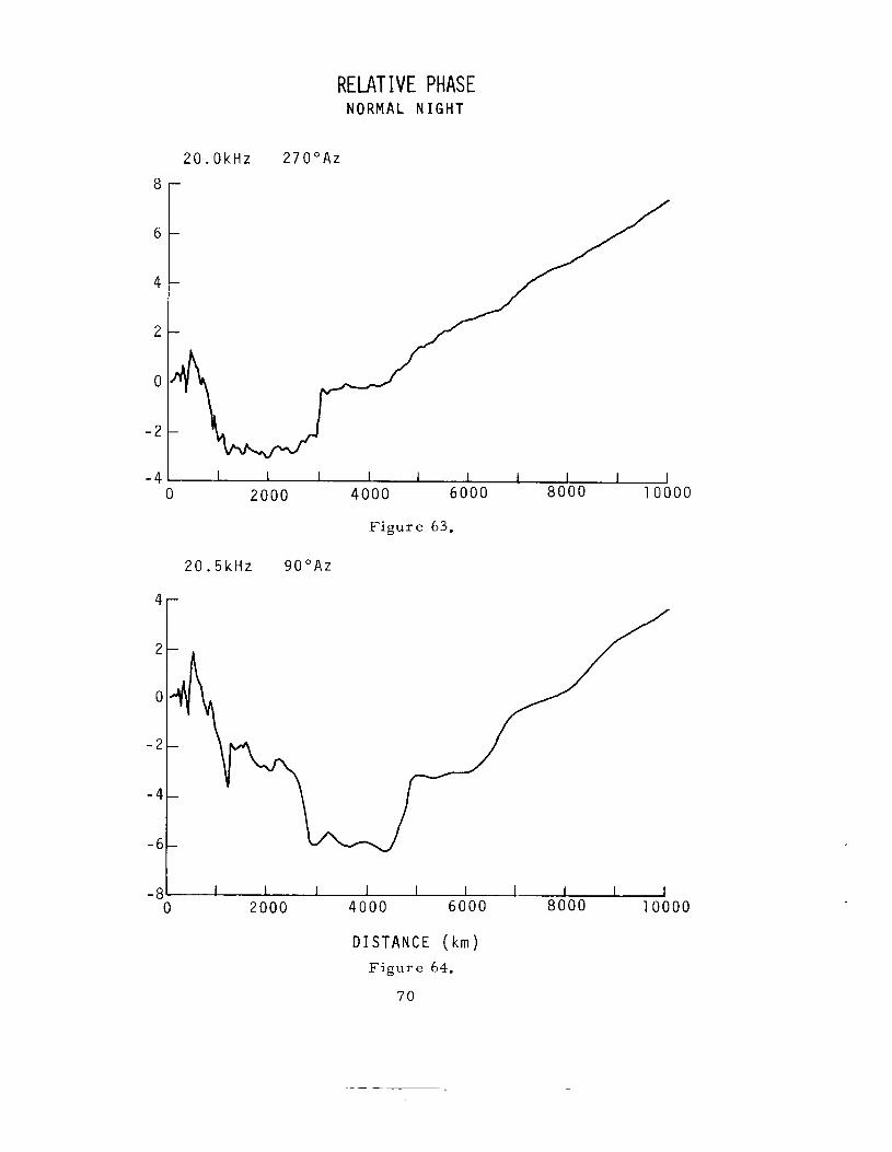
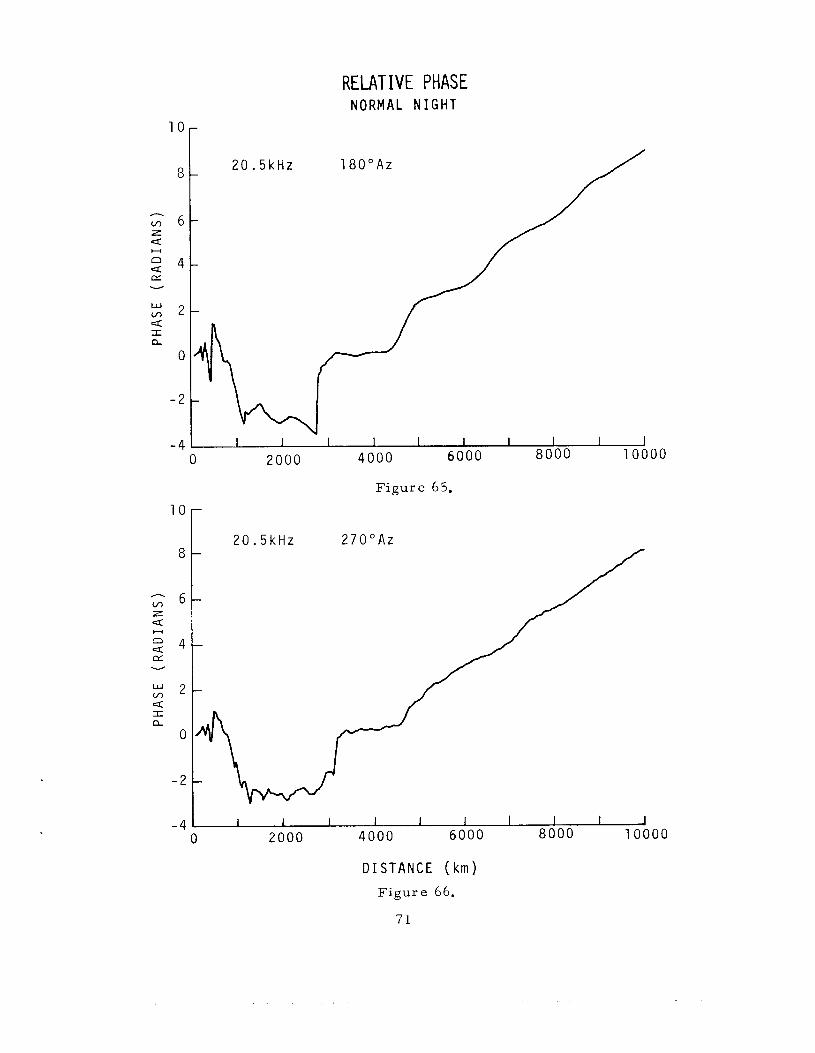
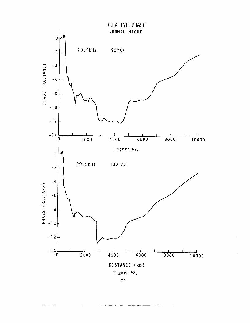
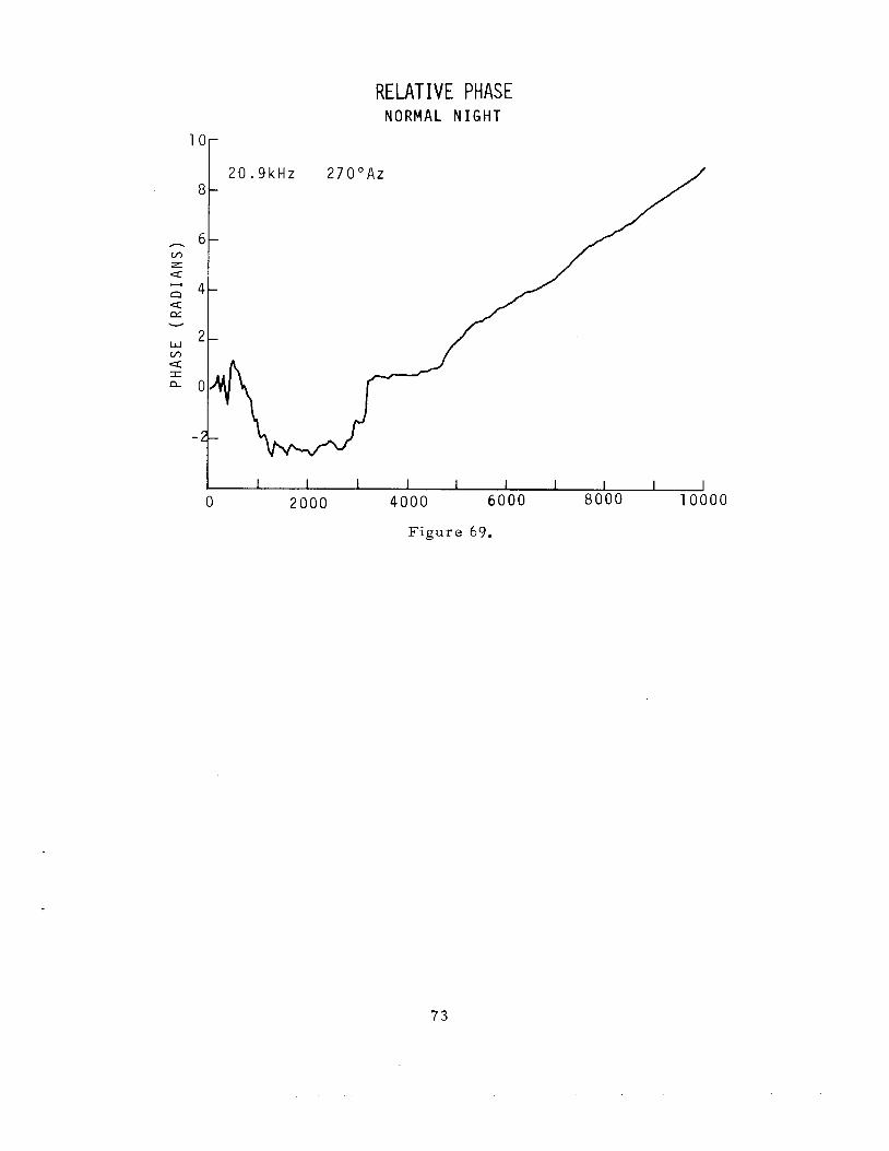
F igu res 8 through 6 9 give a phase cor rec t ion in radians f o r var ious
frequencies and magnet ic az imuths under normal day and no rma l night
conditions.
to the phase delay of a hypothetical wave traveling a t the speed of light
in a medium where the index of re f rac t ion i s 1. 0001.
these f igures a r e labeled "Relative Phase . I '
This phase cor rec t ion is that value which must be added
Consequently,
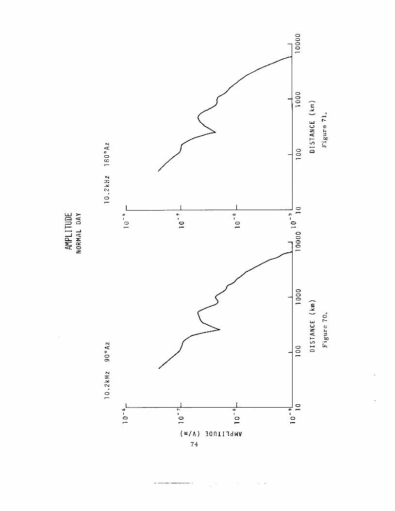
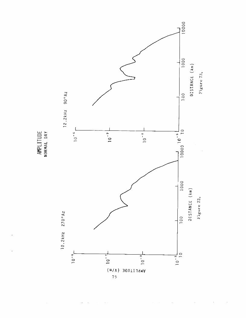
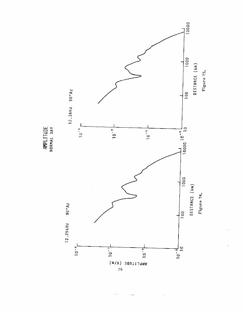
F igu res 70 through 128 give the amplitude in volts p e r m e t e r ,
re fe renced to unity dipole cur ren t , for the var ious frequencies and
azimuths under normal day and no rma l night conditions.
F igu res 129 through 204 give the group delay cor rec t ion in m i c r o -
seconds for var ious frequencies and azimuths under no rma l night
conditions. Again, because this correct ion i s obtained a s the difference
between the absolute group delay and the delay of a wave traveling a t
the speed of light and an index of refract ion of 1.0001, the f igures a r e
labeled "Relative Group Delay. I '
this group delay has been developed by F e y and LooneyZ1 and is analogous
to the method presented e a r l i e r in the text.
The actual method of calculation of
F igu res 205 through 233, "Diurnal Phase , ' I give the phase shift to
be expected between night and day using the no rma l day and n o r m a l
night prof i les .
F igu res 234 through 2 5 4 a r e special c a s e s of the previous calcula-
tions in that e i ther the profile o r ground conditions a r e changed f r o m
previous f igures for the same frequency and azimuth.
7. Discussion and Conclusions
The ana lys i s of the theoret ical data presented h e r e i s a imed a t
It should be noted during the analysis of these timing implications.
17
graphs that the calculations have a tendency to de te r iora te with distance.
This does not affect many of the graphs , but at the point where the t rend
towards l inear i ty with increasing dis tance breaks down, the graph should
be d is regarded o r , conversely, the l inear i ty may be extrapolated to
obtain the des i r ed resu l t s .
m o r e t e r m s (hops) in the geometr ic s e r i e s summation.
The cause of the degeneracy i s a need for
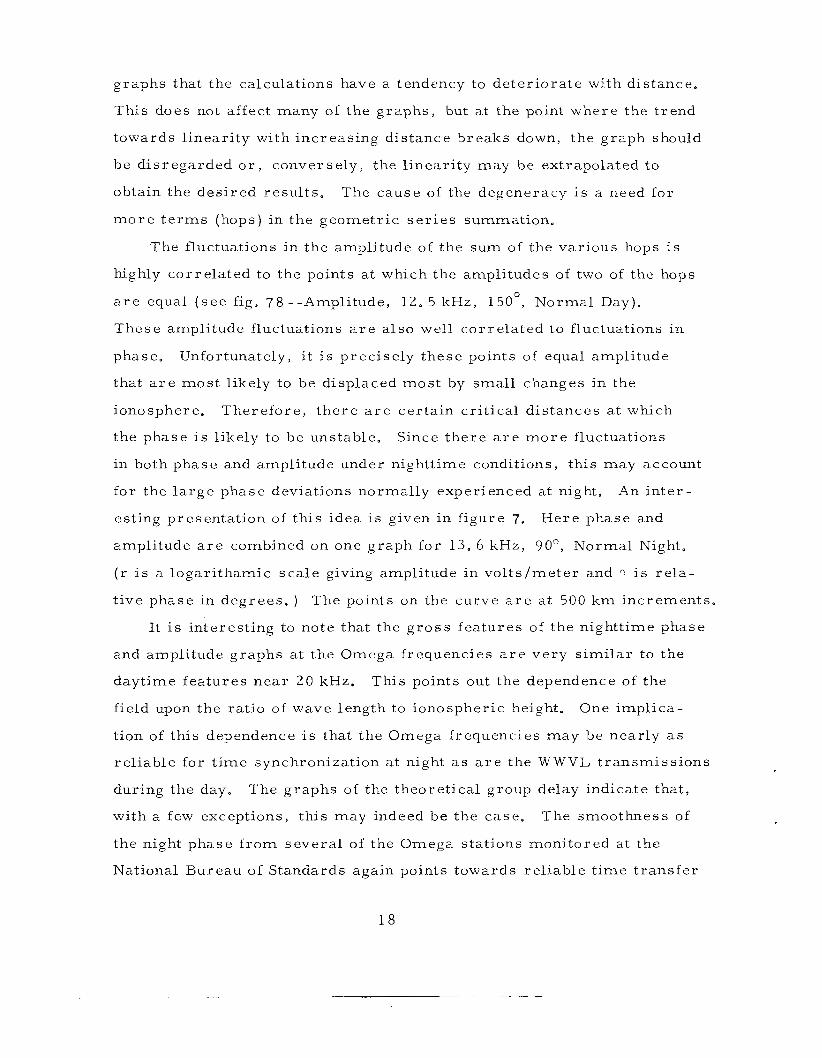
The fluctuations i n the amplitude of the sum of the var ious hops i s
highly cor re la ted to the points at which the amplitudes of two of the hops
a r e equal ( s e e fig. 78--Ampli tude, 12. 5 kHz, 150°, Normal Day).
These amplitude fluctuations a r e a l so well cor re la ted to fluctuations i n
phase. Unfortunately, it is prec ise ly these points of equal amplitude
that a r e mos t likely to be displaced mos t by smal l changes in the
ionosphere. Therefore , t h e r e a r e cer ta in c r i t i ca l dis tances at which
the phase i s likely to be unstable.
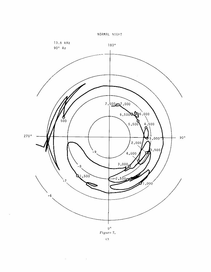
i n both phase and amplitude under nighttime conditions, th i s may account
for the l a r g e phase deviations normally experienced at night,
esting presentation of th i s idea i s given in f igure 7.
amplitude a r e combined on one graph fo r 130 6 kHz, 90”, Normal Night.
( r i s a logari thamic s c a l e giving amplitude in vo l t s /me te r and
t ive phase in degrees . )
Since t h e r e a r e m o r e fluctuations
An i n t e r -
Here phase and
is r e l a -
The points on the curve a r e a t 500 k m increments .
I t is interest ing to note that the g r o s s fea tures of the nighttime phase
and amplitude graphs at the Omega frequencies a r e ve ry similar to the
dayt ime fea tures nea r 2 0 kHz.
field upon the ra t io of wave length to ionospheric height. One implica-
tion of this dependence i s that the Omega frequencies may be near ly as
rel iable for t ime synchronization at night as a r e the W W V L t ransmiss ions
during the day.
with a few exceptions, this may indeed be the case.
the night phase f rom s e v e r a l of the Omega stations monitored a t the
National Bureau of Standards again points towards rel iable t ime t r a n s f e r
This points out the dependence of the
The graphs of the theoret ical group delay indicate that ,
The smoothness of
1 8
during the night a t t hese frequencies. Near 20 kHz, however, i t i s
apparent that synchronization cannot be accomplished with any degree
of reliabil i ty during the night.
During the day, synchronization a t the Omega frequencies should
be very reliable.
a r e diss ipated in near ly all c a s e s by approximately 2 , 000 km.
this point on the group delay becomes near ly l inear and ve ry predictable,
The small fluctuations in the group delay g raphs
From
Onc is able to a r r i v e a t a n es t imate of the maximum timing e r r o r
to be expected using a given pa i r of f requencies , by examining the
group delay plots.
which a r e s imi l a r to damped sine waves.
is then the maximum expected e r r o r .
k i lometers ,
a .
In the majori ty of c a s e s these plots have fluctuations
The amplitude of these waves
Neglecting the first 500 to 1000
the folLowing e s t ima tes of maximum timing e r r o r a r e given:
for the Omega frequencies during the day the expected e r r o r
i s approximately + 2 0 p s e c ;
b. for the frequencies near 2 0 kHz during the day, approximately
f 50 I lsec;
c. for the Omega frequencies a t night, approximate
d. for the frequencies near 2 0 kHz during the night,
* 1 2 0 Usec.
Because of the s imi la r i ty of the relat ive phase grapl
y * 7 0 Usec;
app r oxima t ely
s with changes
in azimuth i t appea r s that l inear interpolation may be used for both
azimuth and dis tance f r o m the t r ansmi t t e r during the day. The night
phase, though,is not near ly so well behaved. In fact , the night phase
a t 2700 i s ve ry d i s s imi l a r to the 90" and the 180° phases (which a r e
r a the r alike).
whether these changes take place l inear ly with azimuth.
A possible a r e a for fur ther study would be to de t e rmine
19
The fluctuations (high frequency Four i e r component) in group delay
Wide frequency a r e very much cor re la ted to the frequency separation.
separat ions have fewer and sma l l e r fluctuations than do na r row f r e -
quency separations.
high resolution and subsequently l a r g e ambiguities of wide separat ions ,
and the low resolution but smal l ambiguity of smal l separations.
At s o m e point then, one mus t choose between the
The Omega navigation sys tem, with i t s proposed worldwide cover - age, has g rea t potential a s a t ime synchronization tool.
of f requencies and frequency separat ion, coupled with the possibil i ty of
24-hour utilization, available a t each of the eight stations in the network
offer medium to high resolution t ime synchronization to a lmos t a l l
l o cal e s .
The var ie ty
I
2 0
8. References
[41
[ 51
C61
[71
Blamont, J. E . , and de J a g e r , C . , "Upper -a tmospheric turbulence determined by means of rockets , I f J. Geophys. R e s . , 67, No. 8, pp. 3113-3119, July 1 9 6 2 .
-
Greenhow, J. S. , and Neufeld, E. L. , "Large sca l e i r r egu la r i t i e s in high al t i tude winds, I ' P r o c . Phys. S O C . , 75, pp. 228-234, 1960. - Manring, E . , Bedinger, J. F., and Knaflich, H. , "Measurements of winds in the upper a tmosphere during Apri l 1961, J. Geophys. R e s . , 67, No. 10, pp. 3923-3925, September 1962. - Charney, J. G., and Drazin, P. G . , "Propagation of planetary- sca le dis turbances f r o m the lower into the upper a tmosphere , I t
J . Geophys. Res., 66, No. 1, pp. 83-109, January 1961. - Crombie, D. D . , "Effects of n o r m a l ionospheric fluctuations on propagation of V L F s ignals to g r e a t dis tances , I t
Instability in Electromagnet ic Wave Propagation (AGARD-EWP Sym. , Ankara, Turkey, October 4-12, 1967), AGARD Conf. P r o c . No. 33, K. Davies (Ed. ), pp. 35-43 (Technivision Serv ices , Slough, England, July 1970).
Phase and Frequency
Rice , S. O . , "Statist ical f luctuations of rad io field strength far beyond the hor izon ," P r o c . IRE, 41, No. 2 , pp. 274-281, F e b r u a r y 1953.
-
Hargreaves , J . K . , "Random fluctuations in VLF s igna ls ref lected obliquely f r o m the ionosphere, 3 . Atmos. T e r r . P h y s . , 20, pp. 155-166, 1961.
-
Hines, C. O., ) ' Internal gravi ty waves a t ionospheric heights, ' I
Can. J. P h y s . , 38, No. 11, pp. 1441-1481, November 1960. - Wait, J . R., and Spies, K . P., "Character is t ics of the e a r t h - ionosphere waveguide fo r VLF rad io waves, Nat. Bur . Stand. (U . s. ) Tech. Note 300, 1964. 1 s t Suppl., F e b r u a r y 1965; 2nd Suppl., March 1965.
Johler , J . R., "On the ana lys i s of LF ionospheric rad io propagation phenomena, J . R e s . , 65D, No. 5, pp. 507-529, September-October 1961.
-
2 1
Johler , J . R . , and Ber ry , L. A . , "Propagation of t e r r e s t r i a l rad io waves of long wavelength- -theory of zonal harmonics with improved summation techniques, IT J. R e s . , 66D, No. 6 , pp. 737 - 773, November-December 1962.
-
Johler , J . R . , "Concerning l imitat ions and fur ther cor rec t ions to geometr ic-opt ical theory for LF, V L F propagation between the ionosphere and the ground, Radio Sci. J . R e s . , NBS/USNC- URSI, - 68D, No. 1, pp. 67-78, January 1964.
Johler , J . R . , "Zonal ha rmon ics in low frequency t e r r e s t r i a l rad io wave propagation, Nat. Bur. Stand. (U. S. ) Tech. Note 335, Apr i l 13, 1966.
Johler , J . R . , "Theory of propagation of low frequency t e r r e s t r i a l radio waves - -mathemat ica l interpretat ion of D-region propagation s tudies , I t ESSA Tech. Repor t IER48-ITSA 47, August 1967.
Johler , J . R. , and Mellecker , C . , "Theoret ical LF , V L F field calculations with spher ica l wave functions of integer o r d e r , ESSA Tech. Report , ERL165-ITS 106, Apr i l 1970.
Debye, P . , "Der l ichtdruck auf kugeln von beleibigem mate r i a l , (English t ranslat ion: "The p r e s s u r e of light on sphe res made of any mater ia l . ' I ) , Ann. Physik (Leipzig), - 30, pp. 57-136, 1909.
Lord Rayleigh, "On the acoust ic shadow of a sphere, I ' with Appendix giving the values of Legendre ' s functions f r o m P 0 Pz0 a t in te rva ls of 5 degrees by Prof . A. Lodge, Phil . Trans . Roy. SOC. , London, A203, pp. 87-110, 1904.
to
Joh le r , J . R., "Ground wave propagation in a no rma l and a n ionized a tmosphere , ESSA Tech. Report , ERL121-ITS 85, 1969a.
Deeks, D. G. , "D-region e lec t ron distributions in middle lati tudes deduced from the ref lexion of long rad io waves, I t P r o c . Roy. SOC., A291, pp. 413-437, 1966. - Bain, W. C . , and May, B. R . , "D-region electron-densi ty dis t r ibut ions f r o m propagation data, P r o c . IEE, - 114, No. 11, pp. 1593-1597, November 1967.
[21] Fey, L., and Looney, C. H . , J r . , "A dual frequency VLF timing sys tem, IEEE Trans . Instrum. and Meas . , IM-15. No. 4, pp. 190- 195, December 1966.
2 2
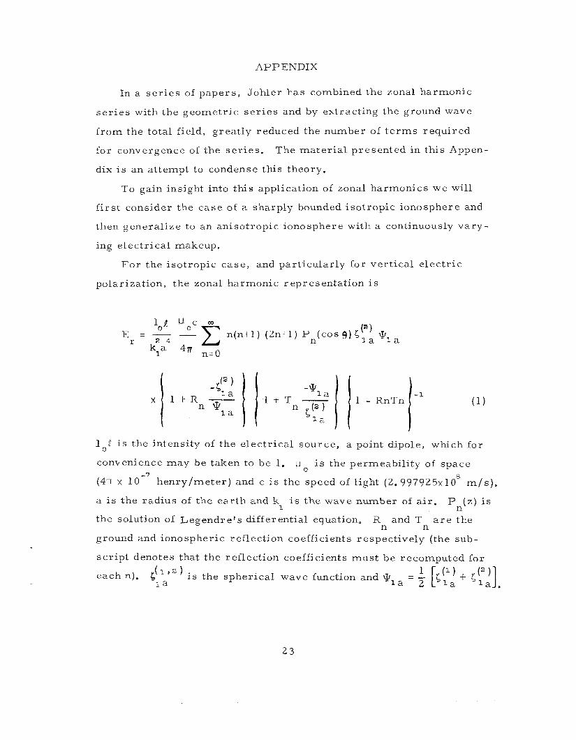
A P P E N D I X
In a s e r i e s of pape r s , Johler has combined the zonal harmonic
ser ies with the geometr ic s e r i e s and by extracting the ground wave
f r o m the total field, great ly reduced the number of t e r m s required
for convergence of the se r i e s .
dix i s an attempt to condense this theory.
The ma te r i a l presented in this Appen-
To gain insight into this application of zonal harmonics we wi l l
f i r s t consider the case of a sharply bounded isotropic ionosphere and
then general ize to an anisotropic ionosphere with a continuously va ry -
ing electr ical makeup.
For the isotropic case , and par t icular ly for ver t ica l e lec t r ic
polarization, the zonal harmonic representat ion i s
I o P is the intensity of the electr ical source , a point dipole, which for
convenience may be taken to be 1.
(4n x
a i s the radius of the ea r th and k
p o is the permeabili ty of space 8
henry /me te r ) and c is the speed of light (2 .997925~10 m / s ) .
is the wave number of a i r . P ( z ) i s 1 n
the solution of Legendre’s differential equation. R and T a r e the n n
ground and ionospheric reflection coefficients respectively (the sub-
scr ip t denotes that the reflection coefficients m u s t be recomputed for
r! ” ’ i s the spherical wave function and a = - each n). la
2 3
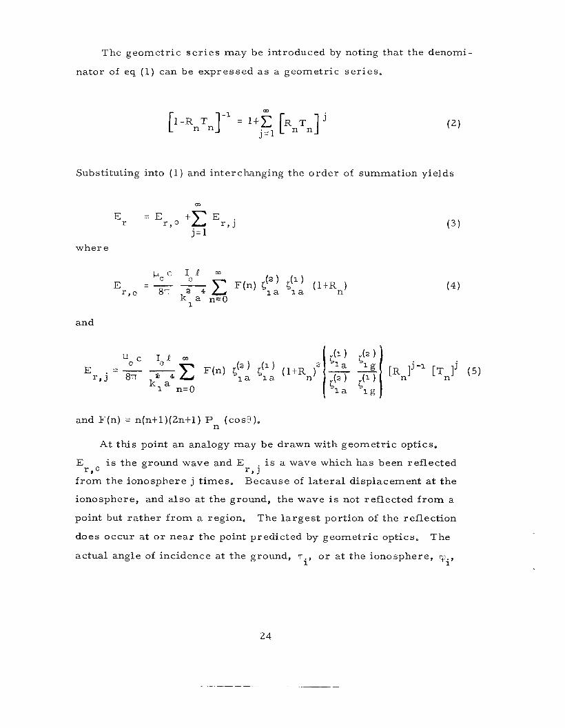
The geometr ic s e r i e s may be introduced by noting that the denomi-
nator of eq (1) can be expressed a s a geometr ic s e r i e s .
[ l-RnTn]' l m [RnTn] j
j = l
Substituting into (1) and interchanging the o r d e r of summation yields
m
+E E r , j = E
r r , o E
j = 1
where
and
( 3 )
and F ( n ) = n(n t1 )
At th i s point
2 n t l ) P ( c o s B ) . n
an analogy may be drawn with geometr ic optics.
E . i s a wave which has been ref lected
f r o m the ionosphere j t imes, Because of l a t e ra l displacement at the
ionosphere, and a l so at the ground, the wave is not reflected f r o m a
point but r a the r f r o m a region. The l a r g e s t portion of the reflection
does occur a t o r nea r the point predicted by geometr ic optics.
actual angle of incidence at the ground, T., o r a t the ionosphere, vi,
i s the ground wave and E r , o r , J
The
1
2 4
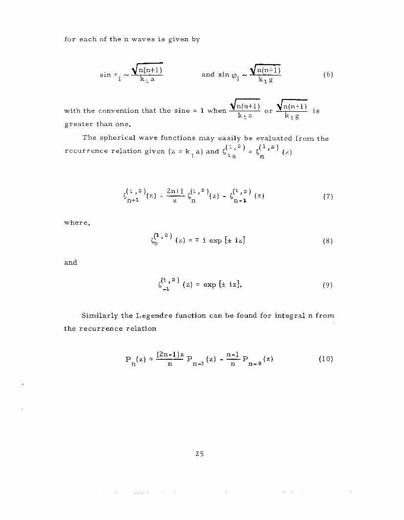
for each of the n waves is given by
with the convention that the s ine = 1 when
g rea t e r than one,
The spherical wave functions may easi ly be evaluated f r o m the
r e c u r r e n c e relat ion given (z = k a ) and ( l Y 2 ) - pq (z) - 1 l a n
where ,
and
( z ) - ( z ) 2 n t l ( 1 ~ 2 )
n n - i (z) = - t; j ( L 2 )
n t l Z ( 7 )
( 9 1 ( z ) = exp [* iz]. 5" $ 2 ) -1
Simi la r ly the Legendre function can be found for in tegra l n f r o m
the r e c u r r e n c e relat ion
p ( z ) P ( z ) = P ( z ) - - (2n - l ) z n-1 n n n -1 n n-2
2 5
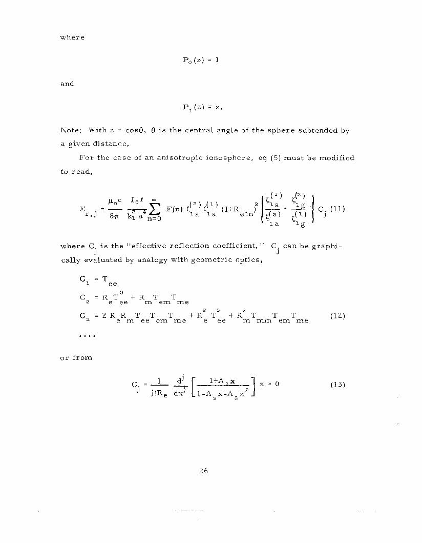
where
P,(z) = 1
and
Note:
a given distance.
With z = cosf3, 8 is the central angle of the sphere subtended by
F o r the case of an anisotropic ionosphere, eq ( 5 ) m u s t be modified
to r ead ,
where C. i s the “effective reflection coefficient.”
cally evaluated by analogy with geometr ic optics,
C . can be graphi- J J
C, = T ee 2
C z = R T t R T T e ee m e m m e
C , = Z R R T T T t R 2 T 3 e ee ~ R ’ T m mm T e m T m e (12) e m ee e m m e
o r f r o m
26
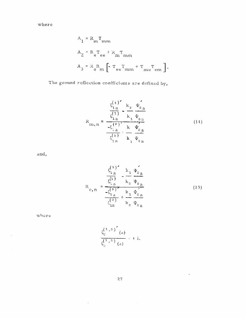
where
A = R T 1 m mm
A = R T tR T 2 e e e m mm
A = R R f T T 3 e m [ - T ee mm m e e m
The ground reflection coefficients are defined by,
and,
where
27
Note that
Since m o s t of the reflection takes place near the points predicted
by geometr ic optics the concept of local reflection coefficients may be
introduced in the expression for C.. J
ground p a r a m e t e r s along the propagation path may be included in the
field equation.
Tha t i s , changes in ionospheric o r
The convergence of the zonal harmonic s e r i e s ( 1 ) i s notoriously
slow pr imar i ly because of the inclusion of the groundwave in this
expression. Equation ( 3 ) , however, s epa ra t e s the groundwave, E r , 0,
f r o m the skywaves.
groundwave, the number of t e r m s requi red for convergence may be
reduced by a factor of approximately 15.
skywave s e r i e s occurs rapidly as n approaches k, a ( s in qi -+ l ) ,
whereas for the groundwave 15 k , a t e r m s a r e required.
the contribution of t e r m s with small angles of incidence, 'pi < 30 , a r e
near ly negligible so that for f requencies up to 20 kHz, only a few hun-
d red t e r m s may be required for convergence.
By using other methods of calculation for the
That i s , convergence of the
F u r t h e r m o r e , 0
2 8
TABLE 1
LIST O F CALCULATIONS
Magnetic Azimuth (Degrees )
10.20 10.20 10.20 10.20 10 ,20 10.20
12.20 12.20
12.25 12.25
12.30 12.30
12. 50 12. 50 12, 50 12. 50 12. 50 12. 50 12. 50 12. 50 12.50 12. 50
12.70 12.70 12.70 12.70 12.70 12.70 12.70 12.70 12,70 12.70
9 0 90
180 180 27 0 270
90 9 0
90 90
90 9 0
90 90
135 135 150 180 180 225 270 270
9 0 9 0
135 135 150 180 180 225 270 270
P r o f i l e Identification
Normal Day Normal Night Norma l Day Normal Night Normal Day Normal Night
Norma l Day Normal Night
Normal Day Normal Night
Norma l Day Normal Night
Norma l Day Normal Night Norma l Day Normal Night Norma l Day Normal Day Normal Night Normal Day Normal Day Normal Night
Norma l Day Normal Night Norma l Day Normal Night Normal Day Normal Day Normal Night Norma l Day Normal Day Normal Night
2 9
TABLE 1 (Continued)
Frequency
(kHz)
13. 60 13.60 13. 60 13.60 13.60 13.60
19.90 19.90 19.90 19.90 19.90 19.90
20,OO 20.00 20.00 20.00 20.00 20.00
20. 50 20. 50 20. 50 20. 50 20. 50 20. 50
20.90 20.90 20,90 20.90 20.90 20.90
10.20 12. 50 12.70 20.00
Magnetic Azimuth (Degrees)
9 0 90
180 180 270 270
90 90
180 180 270 270
90 90
180 180 270 270
90 90
180 180 270 270
90 9 0
180 180 270 27 0
90 90 90 90
P r o f i l e Identification
Normal Day Normal Night Norma l Day Normal Night Norma l Day Normal Night
Norma l Day Normal Night Norma l Day Normal Night Norma l Day Normal Night
Norma l Day Normal Night Norma l Day Normal Night Norma l Day Normal Night
Normal Day Normal Night Norma l Day Normal Night Norma l Day Normal Night
Norma l Day Normal Night Norma l Day Normal Night Normal Day Normal Night
Deeks 1200 Deeks 1200 Deeks 1200 Deeks 1200
30
TABLE 1 (Continued)
1 0 . 2 0 1 2 . 5 0 12.70 2 0 . 0 0
10.20
12. 50
12.70
2 0 . 0 0
12.20
12.20
12.20
12.20
12 .30
12.30
12.30
12.30
Magnetic Azimuth (Degrees)
90 90 90 90
9 0
90
90
90
90
90
90
90
90
90
90
90
Profi le Identification
Bain & May Bain & May Bain & May Bain & May
Normal Day (Sea W a t e r ) Normal Day (Sea Water ) Normal Day (Sea W a t e r ) Normal Day (Sea Water )
Normal Day (Raised 2. 5 k m )
Normal Day (Lowered 2. 5 k m )
Normal Night (Raised 2. 5 km)
Normal Night (Lowered 2. 5 km)
Normal Day (Raised 2. 5 km)
Normal Day (Lowered 2. 5 km)
Normal Night (Raised 2. 5 km)
Normal Night (Lowered 2, 5 km)
31
In
0 N \
0 0 0 0 0 0 0 0 0 0 0 0 0 0 0 0 0 0 "
N N N N N N ~ N N N N N N N N N N N N ~
. . o o o o o o d d d d d d d d d d d d o o o o o o o m
c,
d .* 2 c,
d cd 0 a d k c,
5
2 a, (I]
a
32
d
d
9 m
0 N,
W
Ln M co N,
m 00 Ln M
N
0 ri
d 0 2 $
0 a
M w
3 3
References for Table 2
1. W , D. Westfall, "Diurnal Changes of P h a s e and Group Velocity of V L F Radio Waves, I ' Radio Science, Vol. 2 (New S e r i e s ) , No. 1 , January 1967.
2. B. E. Blair and A . H. Morgan, "Control of W W V and WWVH Standard Frequency Broadcas ts by V L F and LF Signals, Science J. of Res. NBS/USNC-URSI, Vol 69D, No. 7, July 1965,
Radio
3 . Yoshiyuki Yasuda, pr iva te communication.
4. P o B. Rao and W. A. Teso , "An Investigation of Propagat ion P h a s e Changes at V L F , " The Radio and Electronic Engineer, November 19 66.
5. A . L. el Sayed, "Comparison of W W V L and the Local Standard, P r o c . of the Mathematical and Phys ica l Society, U . A . R. , 1969.
6. Measurements m a d e by NBSBL.
7. J . H. Roeder , unpublished report .
34
r- m m m N
.rl u a, k
r- N H
0
0 cv
0
0 N
0 0 0 N N N
d X w
0 0 0 * e a
ln N 3
m 0 4
0 0 0 “ N Gc
0 z 0 E? d 4
0 u 9 4 4 4 > > >
3 3 3 3 3 3
4 > 4 > 3 3
3 3 \
C
35
P
N m m b
v 9
m N
d
cr) M
cr) cr) Ln 4
0 0 r-
b m L n N cr)
m N
N 4
0
Ln v
0
F 0 d
m 9
cr, N 0 * N N
Lo
* co
N
* Ln d
co a 0 d
b u E; w d Pi
J
3 E 2
\
C
4
3 L 2
\ C
36
Lo r- 6 Ln 9 M 9 0 m N
a 0
* co M 9 3 9 3 N
N 0
N d r- 3
6 * A N
0
Q
m 3
0
V 6 d 3
0 N Lo M
* aJ 3 r- N
V
3 3
N
M V
M M \o 6 N
3
r- M N
M N M ?I N 4
J F + \ z 3 c 3
F z \
C
o o m m m r - 6000" 3 N N N 4 3
0 0 0 . 0 0
O \ o m o \ m r - 6000" 3 N N N 3 3
. e - . * .
(I)
k e, 5
E 2 01
2 tf
37

b
m r- m Lo N
co a 0 d
m o N U 7 d * N
O D
* a m N
4
0
r- 0 d
m a . . m N o w N N
a a .d k
: 38
Ld k k a, P G Ld u
c
a, V
2
q .A v 3
" m .d
" - a, a 0 a, U
a a,
4
0 0- r- M
N 4
r- 4 N
* .
Z M M d '
O M a m N
0 0
39
k a, c, c,
3 (I) " rd
b k
m c r ) w c o 4 P - N
. e
0
a Ln 4
* 4 4 N
z $ c 3 \
40
N O R M A L D A Y P R O F I L E
h
V u \ v, z 0 m I- o W -J W u
t I-
m z W
Y
n
4 0 60 80 1 0 0 H E I G H T ( k m )
F i g u r e 1.
D E E K S 1 2 0 0 P R O F I L E
h
V
\ U 2 m z 0 m I- 0
w u
t I-
m
W
c-.l
z o n
- 1 4 0 6 0 8 0 100
H E I G H T ( k m ) F i g u r e 3.
7 5 1 0 0 1 2 5 2 0 0 H E I G H T ( k m )
F i g u r e 2.
B A I N & M A Y P R O F I L E
41 H E I G H T ( k m )
F i g u r e 4.
DI URNAL PHASE 2 0 k H z 1 8 0 " A z
-1oc
lor
\
- T H E O R E T I C A L
a E X P E R I M E N T A L
US
- 2 0
- 3 0
- 4 0 1 I I I I I I I 1 0 0 2 0 0 300 400 5 0 0 600 7 0 0
F i g u r e 5.
40 r 30
20
RELATIVE GROUP DELAY N O R M A L D A Y
2 0 . 0 k H z 1 8 0 " A z 0
0 - T H E O R E T I C A L -1 o E X P E R I M E N T A L
0 0
- 1 0 0 5 0 0 1 , 0 0 0 1 , 5 0 0 2,000
D I S T A N C E ( k m ) F i g u r e 6.
42
1 3 . 6 k H z
9 0 " A z
2 7 0 "
N O R M A L N I G H T
1 8 0 "
RELATIVE PHASE N O R M A L D A Y
1 0 . 2 k H z 9 0 " A z
1 1 I I 1 I 1 I I I 0 2 0 0 0 4 0 0 0 6000 8 0 0 0 1 0 0 0 0
Figure 8.
1 0 . 2 k H z 1 8 0 " A z
1 1 1 1 1 I 1- 0 2 0 0 0 4 0 0 0 6000 8 0 0 0 1 0 0 0 0 -81
D I S T A N C E ( km)
Figure 9.
44
2
0 - v, z Q
4: CT
H
I 3 - 2
v - - 4 v, 4 I a
- 6
-8
RELATIVE PHASE N O R M A L D A Y
1 0 . 2 k H z 2 7 0 " A z
1 I I I 1 1 1 I I J 0 2000 4 0 0 0 6000 8 0 0 0 1 0 0 0 0
F i g u r e 10.
1 2 . 2 k H z 9 0 " A z
w - 2 1 v,
- 4 -1 0 2 0 0 0 4 0 0 0 6 0 0 0 8000 1 0 0 0 0
2 1 I , , I I ,
D I S T A N C E ( k m )
Figure 11
4 5
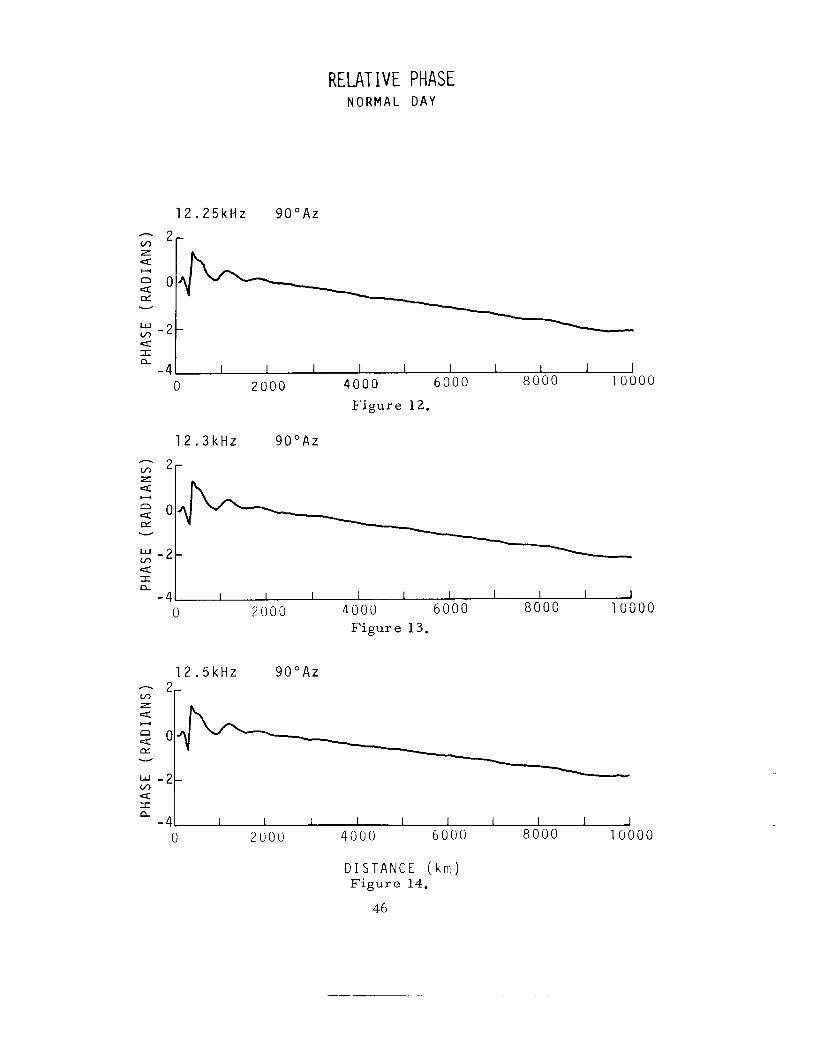
RELATIVE PHASE N O R M A L D A Y
I a
- 4
1 2 . 2 5 k H z 9 0 " A z
2r
I I I I I I 1 1 1 I
1 2 . 3 k H z 9 0 " A z
4 I a
I 1 I 1 1 I 1 I I 1 0 2000 4000 6000 8000 10000
- 4
Figure 13.
1 2 . 5 k tiz 9 0 " A z z 2r z Q
n Q E
H
v
w - v, 4: I a
- 41 I I I 1 I I I I 1 I 0 2000 4000 6000 8000 10000
D I S T A N C E ( k m ) Figure 14.
46

RELATIVE PHASE N O R M A L D A Y
v, Q I a
1 2 . 5 k H z 1 3 5 " A z
Q I a
- v, 2r
1 2 . 5 k H z 1 5 0 " A z
U
v, w - 2 1
1 2 . 5 k H z 1 8 0 " A z
*r
Q I n - 4 I I I I I 1 I I 1 1
0 2000 4000 6000 8000 10000
D I S T A N C E ( k i n )
Figure 17.
47
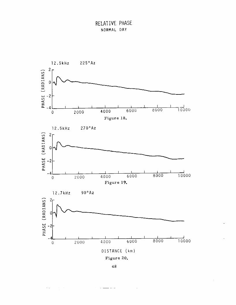
RELATIVE PHASE N O R M A L D A Y
4 I a
1 2 . 5 k H z 2 2 5 " A z
I I I I I I I 1 1 1
r
W
5 I n
m - 2 -
- 4
I I 1 I I I I I I I 6000 8000 100 0 2000 4 0 0 0
I I I I I 1 I 1 I I
Figure 18.
00
1 2 . 7 kHz 9 0 " A z
D I S T A N C E ( k m )
Figure 20.
48
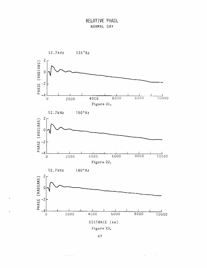
RELATIVE PHASE N O R M A L D A Y
w - 2 - m 4 I n
1 2 . 7 kHz 1 3 5 "Az
1 I I I 1 1 I I I
z 4
r : o 4 ry: v
w - 2 v, Q I a - 4 1 I I I 1 1 I 1 I 1 J
0 2000 4000 6000 8000 100 Figure 21.
- 2 v, z 4:
z o
; - 2
4 ry: v
4 I n - 4
1 2 . 7 kHz 1 5 0 " A z -
00
1 I 1 I 1 1 I 1 I I 0 2000 4000 6000 8000 10000
Figure 22.
1 2 . 7 k H z 1 8 0 " A z
D I S T A N C E ( k m )
Figure 23.
49
RELATIVE PHASE N O R M A L D A Y
w - 2 -
a - 4
v, 5 I
1 2 . 7 kHz 2 2 5 " A z
1 I 1 I I 1 I I 1 I
Figure 24.
1 2 . 7 k H z 2 7 0 " A z
I 1 I 1 I I I I 1 -I 0 2000 4000 6000 8000 10000
Figure 25.
1 3 . 6 k H z 9 0 " A z
I 1 I I 1 1 I I I 0 2000 4000 6000 8000 10000
D I S T A N C E ( k m )
Figure 26.
5 0
RELATIVE PHASE N O R M A L D A Y
1 3 . 6 k H z 1 8 0 " A z
2 - Q
Q I a I 1 I 1 I 1 I I I I
4000 6000 8000 10000 - 2 0 2000
F i g u r e 27.
13.6kHz 2 7 0 " A z
I 1 1 I I I 1 2 - a 0 2 0 0 0 4000 6 0 0 0 8000 1 0 0 0 0 - 21
D I S T A N C E (km) Figure 28.
51
RELATIVE PHASE N O R M A L D A Y
19.9kHz 1 8 0 " A z
1 I 1 I I 1 I d - 0 2000 4000 6 0 0 0 8 0 0 0 1 0 0 0 0
D I S T A N C E ( k m )
Figure 29.
52
RELATIVE PHASE N O R M A L D A Y
1 9 . 9 k H z 9 0 " A Z
- 61 I 1 I I 1 I 1 I I 1 0 2000 4000 6 0 0 0 8000 1 0 0 0 0
Figure 30.
1 9 . 9 k H z 2 7 0 0 ~ ~
- 61 I 1 I 1 I I 1 2 - 0 2000 4000 6000 8000 10000
D I S T A N C E ( k m )
Figure 31.
53
RELATIVE PHASE N O R M A L D A Y
2 0 . OkHz 9 0 " A z
1 1 1 1 1 I 1 1 I I 0 2 0 0 0 4 0 0 0 6 0 0 0 8000 1 0 0 0 0
Figure 32.
20. OkHz 1 8 0 " A z
I 1 I I I I 1 2 - 0 2000 4000 6 0 0 0 8 0 0 0 1 0 0 0 0
D I S T A N C E ( k m )
Figure 3 3 .
54
4
- 2 m z Q
r : o Q CT v
w - 2 m 4 1 a - 4
-6
RELATIVE PHASE N O R M A L D A Y
2 0 . 0 k H z 2 7 0 " A z
-
I 1 1 I 1 I I I I J 2 0 0 0 4000 6 0 0 0 8000 1 0 0 0 0 0
Figure 34.
2 0 . 5 k H z 9 0 " A z
U L U U U s u u u o u u u o v v v I uuuu
D I S T A N C E ( k m )
Figure 35.
55
RELATIVE PHASE N O R M A L D A Y
4
n 2 m z Q
z o Q w v
w - 2 m Q I a - 4
-6
2 0 . 5 k H z -
-
1 8 0 " A z
I I I 1 1 I I I 1 I 0 2 0 0 0 4 0 0 0 6 0 0 0 8 0 0 0 1 0 0 0 0
Figure 36.
4
- 2 m z < E o
w - 2
a w v
m Q I a - 4
- 6
2 0 . 5 kHz -
2 7 0 " A z
I 1 I I 1 I 1-
0 2 0 0 0 4 0 0 0 6 0 0 0 8 0 0 0 1 0 0 0 0
D I S T A N C E (km)
Figure 37.
56
RELATIVE PHASE N O R M A L D A Y
2 0 . 9 k H z 9 0 " A z
1 1 1 1 I I I 1 I I 0 2000 4 0 0 0 6 0 0 0 8000 1 0 0 0 0
Figure 38.
2 0 . 9 k H z 1 8 0 " A z
I 1 1 I 1 - 6' 1 1- 0 2000 4000 6 0 0 0 8 0 0 0 1 0 0 0 0
D I S T A N C E ( k m ) Figure 39.
57
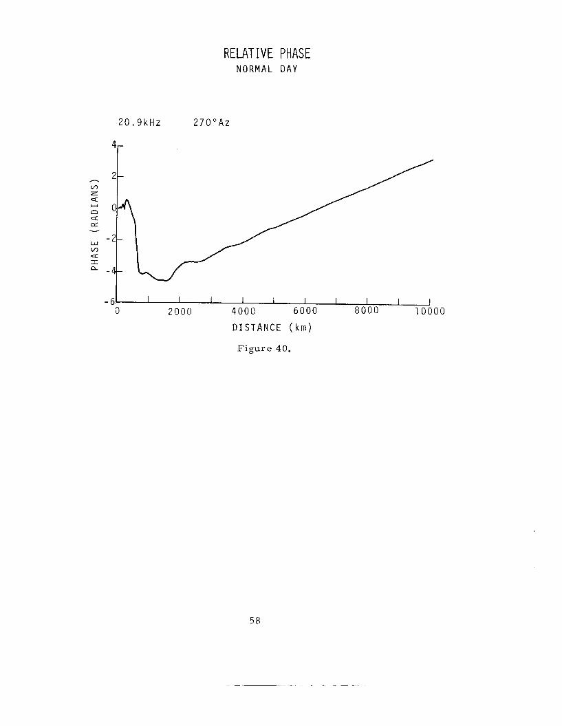
2 0 . 9 k H z
RELATIVE PHASE N O R M A L D A Y
2 7 0 " A z
-6 I 1 I I 1 1 1 I I I 0 2000 4000 6000 8 0 0 0 1 0 0 0 0
D I S T A N C E (k in )
Figure 40.
58
1 0 . 2 k H z
z Q - - 2 - n Q Ly: v
-4 W Ln Q I a - 6 -
- 8
'r
-
1 1 I I I 1 1 I I 1
RELATIVE PHASE N O R M A L N I G H T
9 0 " A z
Figure 41.
1 0 . 2 k H z 1 8 0 " A z
I 1 I I I I I 1 I I 0 2000 4000 6 0 0 0 8 0 0 0 10000
D I S T A N C E ( k m )
Figure 42.
5 9
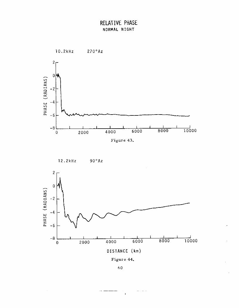
RELATIVE PHASE N O R M A L N I G H T
1 0 . 2 k H z 2 7 0 " A z
I 1 I 1 I I I I I I 4000 6000 8000 10000
-8 1 0 2000
Figure 43.
1 2 . Z k H z Y U " A z
I 1 I I 1 I I I 1 1 2 0 0 0 4000 6000 8000 10000 0
DISTANCE ( km)
Figure 44.
60
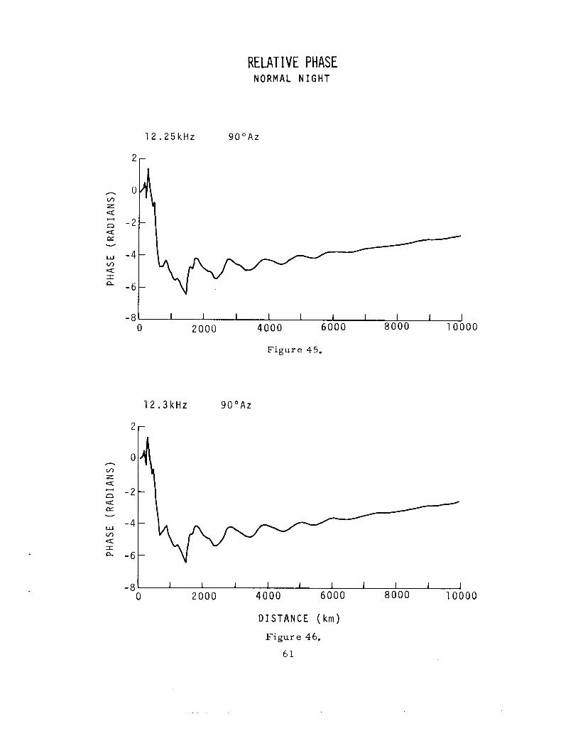
1 2 . 2 5 k H z
RELATIVE PHASE N O R M A L N I G H T
9 0 " A z
-81 I 1 I 1 1 1 1 I 1 I 0 2 0 0 0 4000 6000 8000 10000
Figure 45.
2
0 h
Ln z Q
4 e
- 2
v
- 4 w m 4: I a - 6
-8
1 2 . 3 k H z
-
9 0 " A z
0 2 0 0 0 4000 6000 8000 10000
D I S T A N C E (km)
Figure 46.
61
RELATIVE PHASE N O R M A L N I G H T
1 2 . 5 k H z 9 0 " A z
2,
- v, z 4 H
n 4 m v
w v, 4 I a
I I 1 1 I I I 1 I I 4000 6000 8000 1 0 0 0 0 0 2000
Figure 47.
1 2 . 5 k H z 1 3 5 " A z
1 1 I I 1 I I I I I 0 2 0 0 0 4000 6000 8000 10000
D I S T A N C E (I" F i g u r e 48.
62
RELATIVE PHASE N O R M A L N I G H T
1 2 . 5 k H z 1 8 0 " A z
-81 I 1 I 1 1 I 1 I I 1 0 2 0 0 0 4 0 0 0 6000 8000 1 0 0 0 0
Figure 49.
1 2 . 5 k H z 2 7 0 " A z
I I I I I I I I I I 0 2 0 0 0 4 0 0 0 6 0 0 0 8000 10000
D I S T A N C E ( k m )
Figure 50.
6 3
RELATIVE PHASE N O R M A L N I G H T
- 4
- 6
1 2 . 7 k H z 9 0 " A z
-I W v, Q I n
I I I 1 I I I I I I 0 2000 4000 6000 8000 10000 - 8 I
Figure 51.
2
0 n m z <
ct cr:
U
-2 v
- 4 m Q I n
- 6
-8
1 2 . 7 k H z 1 3 5 " A z
-
-
-
-
1 1 I I 1 1 I 1 I I 0 2000 4000 6000 8000 10000
D I S T A N C E ( k m ) Figure 52.
64
2
0 cn z Q - - 2 n Q & v
-4 W cn Q I a - 6
-8
2
- 0 v, z 4: H
n - 2 4: & v
w -4
n
m Q I
- 6
-8
RELATIVE PHASE N O R M A L N I G H T
1 2 . 7 k H z 1 8 0 O A z
I I I I I I I I I I 0 2000 4000 6000 8000 10000
Figure 53.
1 2 . 7 k H z 2 7 0 " A z
1 I 1 1 1 1 I 1 1 J I 2000 4000 6000 8000 10000
D I S T A N C E ( k m )
Figure 54.
6 5
RELATIVE PHASE N O R M A L N I G H T
1 3 . 6 k H z 9 0 " A z
0 h
m z Q U
- 2 Q CT v
m -4 Q I a
- 6
-8 I
0 2000 4000 6 0 0 0 8 0 0 0 1 0 0 0 0
Figure 55.
2
- 0 m z Q H
n - 2 Q CT v
w -4 m Q I Q
- 6
-8
1 3 . 6 k H z 1 8 0 " A z
I 1 I 1 1 I I I I I 0 2000 4000 6 0 0 0 8000 10000
D I S T A N C E ( k m )
Figure 56.
66
RELATIVE PHASE N O R M A L N I G H T
2
- 0 v, z Q
Q CY
CI
a - 2
v
w -4 v, a 1 a - 6
-8
6
4
2 - v, z 4
G O 4 CY v
- 2 W v, 4 I
-4
- 6
- 8
1 3 . 6 k H z 270'AZ
I 1 1 I I I I I I I 4 0 0 0 6000 8000 1 0 0 0 0 0 2 0 0 0
Figure 57.
1 9 . 9 k H z 9 0 " A z
I 1 I I I I 0 2000 4 0 0 0 6000
D I S T A N C E ( k m )
Figure 58.
6 7
- 8000 10000

RELATIVE PHASE N O R M A L N I G H T
- 2
n
m z 4: H
n 4: CL v
w v, 4: I a
n
v, z Q
c3 4: e
+-I
v
w m Q I a
1 9 . 9 k H z 180"AZ
8
6
4
2
0
- 2
1 9 . 9 k H z
Figure 59.
2 7 0 " A z
- 4 I 1 I 1 1 I I I I I - 0 2000 4 0 0 0 6000 8000 10000
DISTANCE ( k m )
Figure 60.
6 8
RELATIVE PHASE N O R M A L N I G H T
4
2
h
* o z 4
c3 H
2 - 2 v
W m - 4 C t
a - I
- 6
- 8
2 0 . 0 k H z 9 0 " A z -
1C
E
- E m z 4
E 4 Q lx v
w 2 * 5 I a C
- 2
-4
I 1 I I 1 1 I I I I 0 2 0 0 0 4 0 0 0 6000 8 0 0 0 10000
Figure 61. -
2 0 . 0 k H z 1 8 0 " A z
1 I I 1 I I I I I I 0 2 0 0 0 4 0 0 0 6000 8000 1 0 0 0 0
D I S T A N C E ( k m )
Figure 62.
69
RELATIVE PHASE N O R M A L N I G H T
20.0kHz 2 7 0 " A z
8r
I 1 I 1 1 1 I I 1 I 0 2000 4000 6000 8 0 0 0 10000
Figure 63.
2 0 . 5 k H z 9 0 " A z
4
2
0
-2
- 4
- 6
- a I I I I 1 I I 1 I I 0 2000 4 0 0 0 6000 8000 1 0 0 0 0
DISTANCE ( k m ) F i g u r e 64.
70
RELATIVE PHASE N O R M A L N I G H T
I 1 I I I I 1 I 4000 6000 8 0 0 0 1 0 0 0 0 2 0 0 0
1 0
8
- 6 m z Q H
Q n 4
- 2 m
CT v
Q I a
0
-2
- 4
Figure 65. -
0
2 0 . 5 k H z 2 7 0 " A z
I I 1 I I I I 1 I I 0 2000 4000 6000 8000 1 0 0 0 0
D I S T A N C E ( k m )
Figure 66.
RELATIVE PHASE N O R M A L N I G H T
0
-2
- 4 n v, z 4: - -6 n Q e v
-8 w v, 4: I n- - 1 0
- 1 2
- 1 4
20.9kHz 90"Az
Figure 67.
20.9kHz 1 8 0 " A z
I 1 I I 1 I I I I 1 0 2000 4000 6000 8000 10000
00
D I S T A N C E ( k m )
Figure 68.
72
1C
E
E h
m z Q
z 4 Q @L v
2 W m Q I a c
- I
RELATIVE PHASE N O R M A L N I G H T
I I 1 1 1 1 I I I I 0 2 0 0 0 4 0 0 0 6000 8000 1 0 0 0 0
Figure 69.
7 3
(D
I
0 7
N 4 0 0 m
N I Y N
0 c
I 0 -
m I 0 -
I 0 7
I 0 7
( W A ) 3aniiidww 74
0 0 0 0 7
0 0 0
0 0 7
0 0 1 -
0 I
7
0 0 0 0 -
0 0 0 7
0 0 7
0 - I 0 -
N 4: 0 0 m
N I Y N
(u 7
,n I 0 7
t. I
0 7
a,
I 0 7
N 4: 0 0 h N
N I Y N
0 7
1 I I m W r.
I 0 7
0 7
I
0 -
0 0 0 0 7
0 0 0 7
0 0 7
3 m -
0 I -
0 0 0 0 7
0 0 0 7
3 3 -
3 -
h
E 24 v
w V z 4: I- m H
n
h
E Y v
W V L Q I- m u n
I 0 7
rr) r- a,
2 M
.d
Gc
N 4: 0 0 In
N I Y pr)
N -
N 4:
0 m 0
N I Y Lo N
N -
0 0 0 0 7
0 0 0 7
0 0 7
I I I PI m
0
I 0 7
1
0 7
I
0 -
h
E Y v
W V z U I- v,
0 Y
h
E Y v
W V z Q: I- v,
0 CI
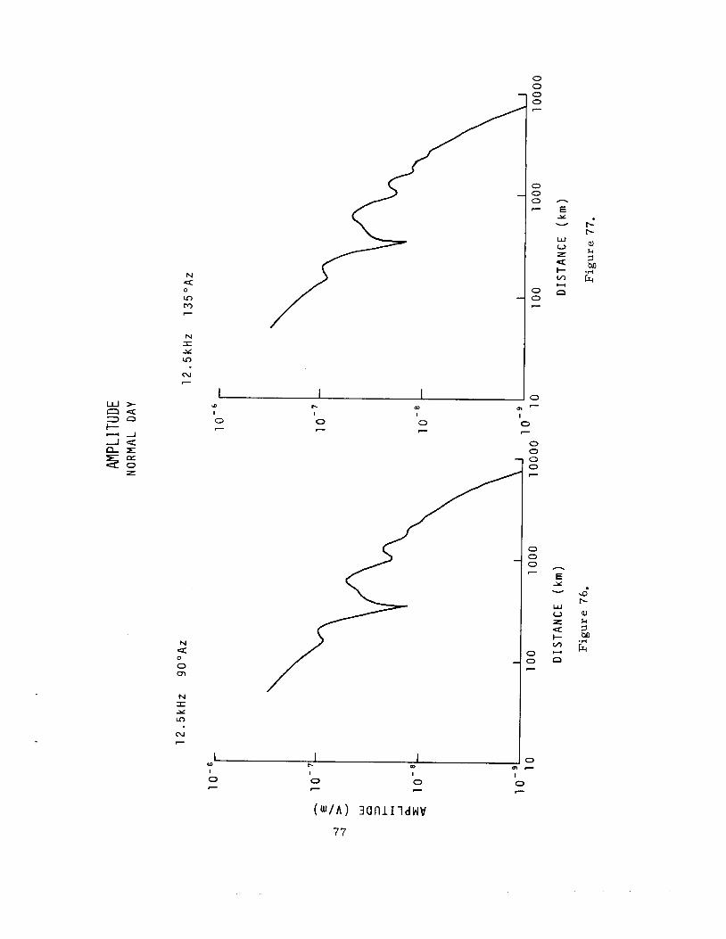
N 4 0
m M - N I Y m
N 7
(0
I
0 7
l- I 0 - m
I
0 7
N 4: 0
0 m
N I Y LrJ
N - 1 I I
I W b (D
0 - 0 7
0 7
0 0 0 0 -
0 0 0 7
0 0 -
0 m -
0 I - 0 0 i;l 0 7
0 0 0 -
0 0 -
0 -
n
Y E v
w V L U I- v, U n
n
Y E v
W V z 4 I- v) U n
0 -
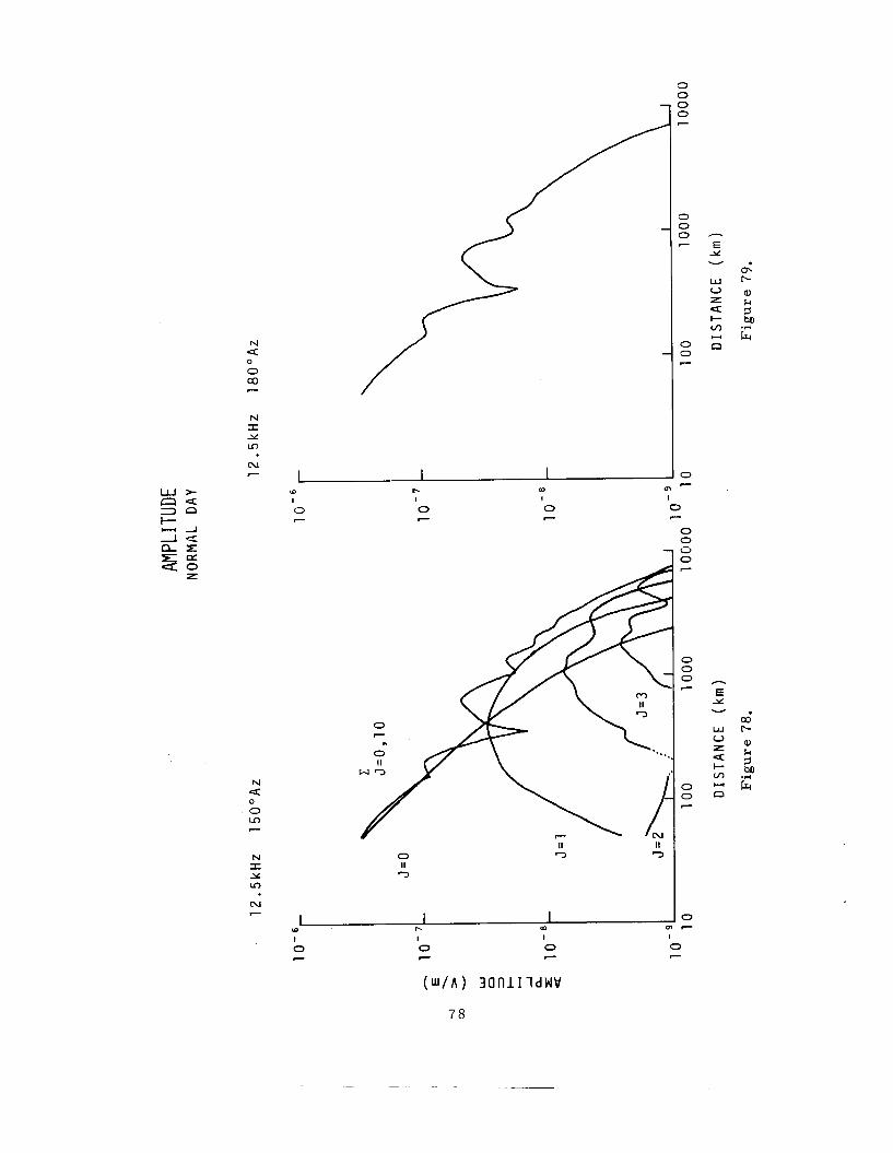
N 4
0 a3
0
7
N I Y LD
N 7
N 4 0 0 In 7
N I 24 LD
N 7
(D
I
0 - b
I
0 c
m I 0 7
0
0 II 3
m -
0 I
7
II 3
II 3
I I 1 (0 PI m
I I C
0 - 0 c
0 - 7 8
0 0 c, 0 7
0 0 0
0 0 7
0 - 0
h
E Y U
W V z Q: I- v, U
n
CI
E Y U
W V z 4 I- v,
0 U
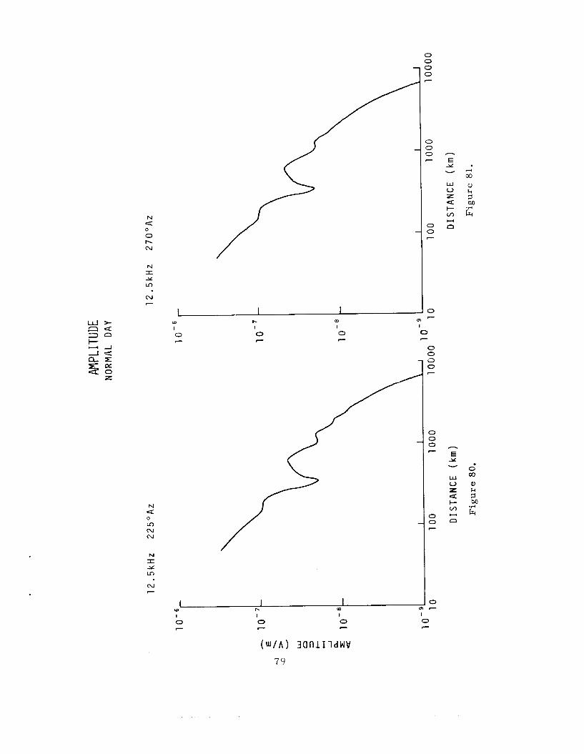
0 0
W r n e =>a
N 4 0 0 h N
N I Y U J
N c
I I I 9 I 0 7
t. I
0 - m I
0 c
N 4 0 m cu N
N I Y Lo
cu 7
L I I W r- m
1 I
0 7
0 .- 0 7
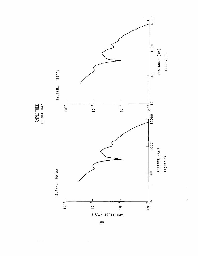
N Q 0 In m - N I Y h
N ?
N 4: 0 0 m
N I Y h
N -
0 0 0 0 7
0 0 0 7
0 0 -
1 I I 3
I I I I. m c n - 0
0 7
0 7
0 - 0 7
0 0
80
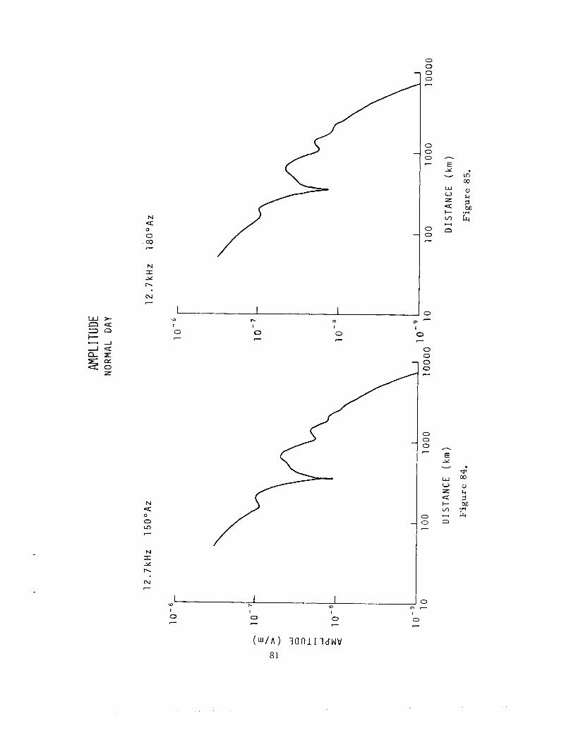
N 4: 0 0 m 7
N I Y h
N -
N 4:
0 co 0
7
N I Y h
N -
I 1 I I W m r.
I I
0 0 0 0 7 7 7 7
( M I A ) 3 0 f l l I l d W V 81
0 0 0 0 7
0 0 0 7
0 0 7
0 0 0 0 7
0 0 0 7
0 0 -
3 -
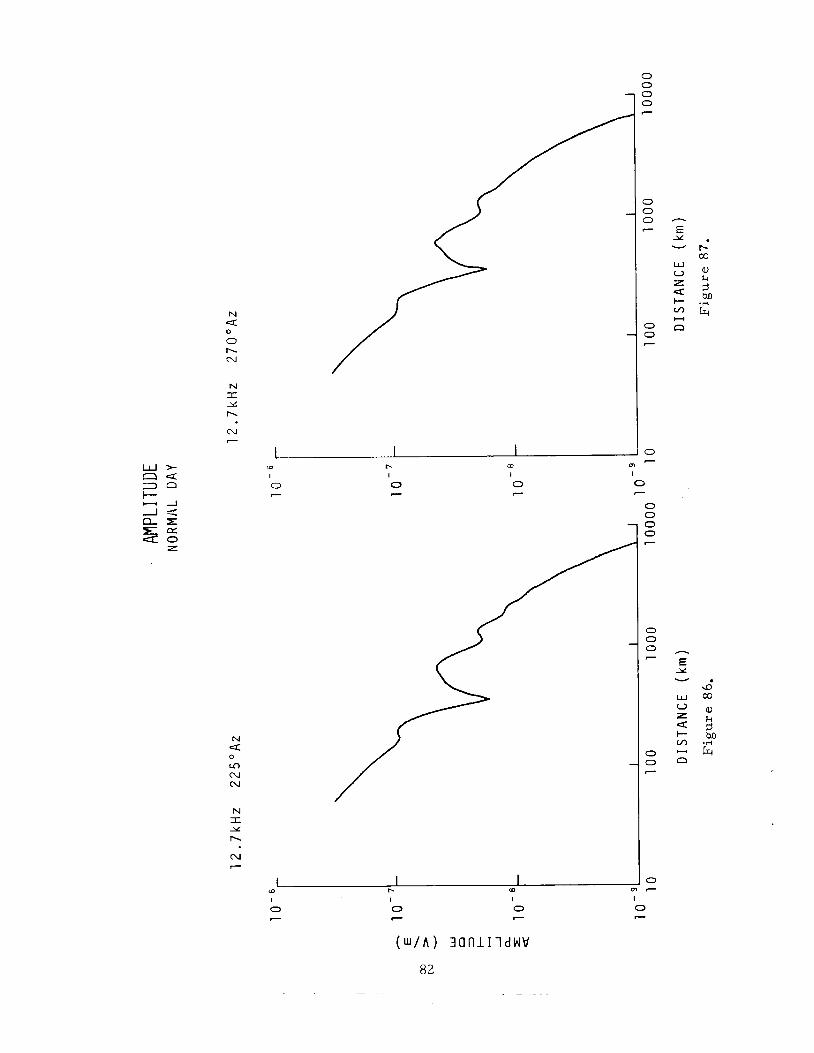
0 0
N Q 0 0 h c\1
N I Y h
c\I 7
0 7
N < 0 Lo (v N
N I Y h
N c
I 0 7
c- I
0 7
I 0 7
I 0 7
82
m y
0 I
7
0 0 0 0 7
0 0 0 7
0 0 c
0 7
I 0 -
h
E Y v
W V z 4 I- m U
n
h
E Y v
w V z 4 i- m U
n
b co a, k 3 M
cr .r(
9 co a, k 1 M
cr .I+
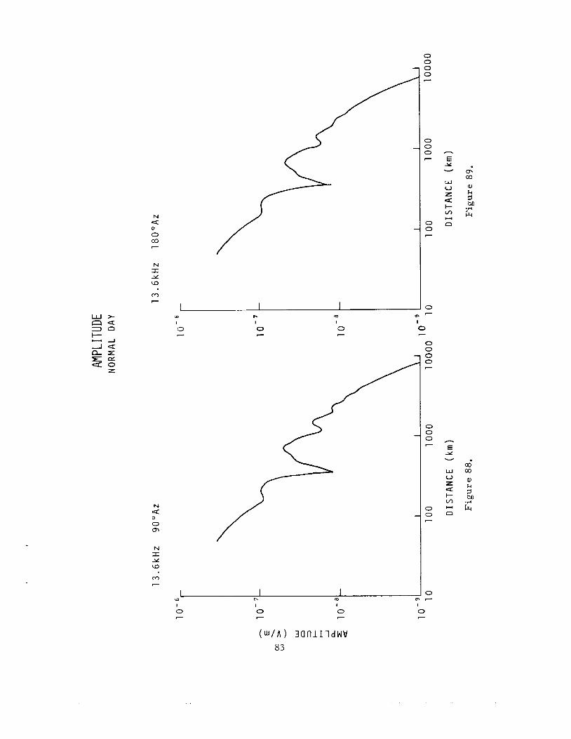
N 4:
0 Q)
0
- N I Y la
m e
N 4
0 0-l
0
N I Y la
m 7
(D
I
0 7
b
I
0 - W
I 0 7
I I I ul PI W
I I I
0 e
0 - 0 e
( W n ) 3 a n i 1 i d w v 83
0 0 0 0 e
0 0 0 e
0 0 e
0 m y
0 I - 0 0 0 0 e
0 0 0 e
0 0 -
0 - 0 7
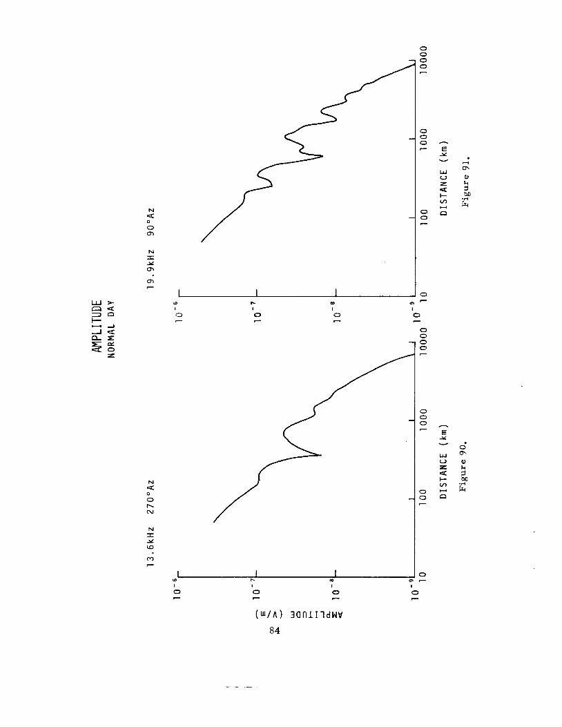
N 4
0 m 0
N I Y m m -
N
0 0 b N
N I 24 10
m
tn I
0 - h I
0 - m I 0 -
I I I W I. m I 0 - I
0 c
I 0 7
0 0 0 0
0 0 0 7
0 0 7
0 m -
0 I
7
0 0 0 0 .-
0 0 0 7
0 0 7
0 7
0 -
h
E Y v
w V L U I- m
c3 U
- E 24 v
W V r 4 I- m Y
n
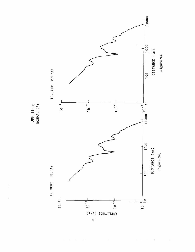
N < 0 0 h N
N I A cn cn 7
N 4:
0 al 0
7
N I Y cn cn 7
(D
I
0 7
I. I 0 - m
I 0 7
0 0 0 0 -
0 0 0 7
0 0 7
0 m -
0 I
F-
I I I p1 m (D
I I I I
0 0 0 0 7 - 7 c
( W / A ) 3ClfllIldWW
0 0 0 0 7
0 0 0 7
3 3 -
3 -
h
E Y v
w V L U I- In 0 CI
h
E Y v
w V z 4: I- v) - n
85
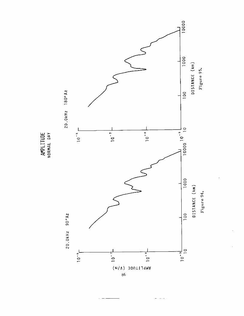
u r a4:
N 4: 0 0 a3 - N I Y 0
0 N
N 4: 0 0 m
N I Y 0
0 N
I 0
a0
I 0 7
I 0 - I
0 - I
0 7
0 0 3 3 -
0 0 0 -
0 0 -
0 cn-
0 I
I---
0 0 0 0 -
0 0 0 -
0 0 7
0 7
I 0 -
- E Y v
W u L < t- m U
n
h
E Y v
W 0 L 4 I- m - n
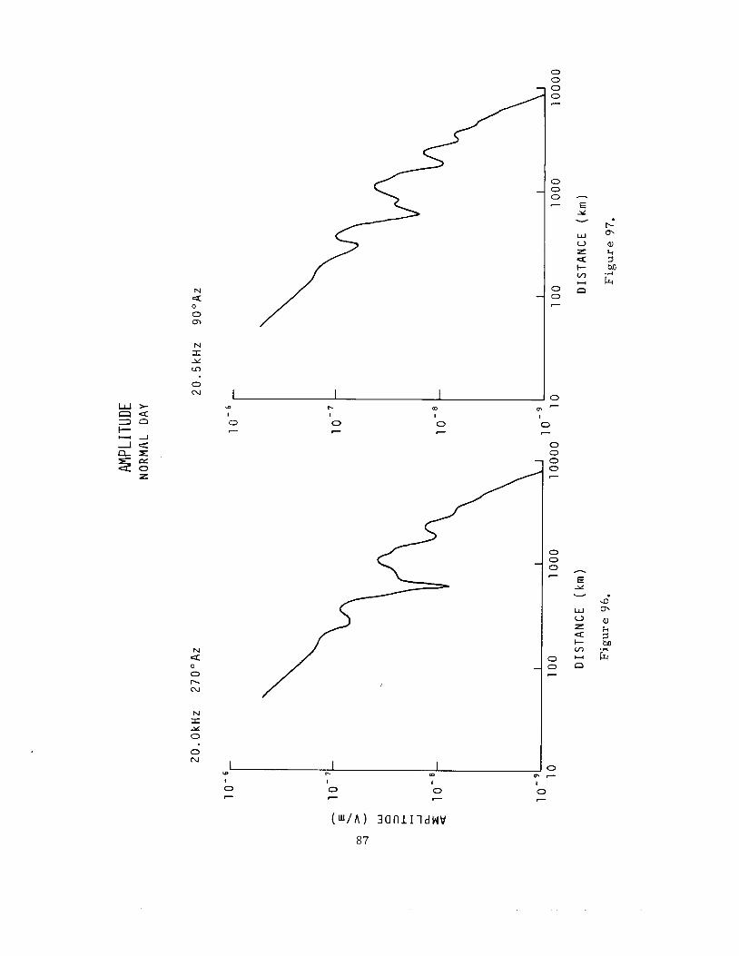
W r n e 3 n
N Q 0 0 m
N I Y In
0 N
(D
I
0 7
N Q 0 0 h cu
N I Y 0
0 N
P- I
0 c
m I
0 7
I I I W I. m I 0 7
0 0 0 0 7
0 0 0 7
0 0 7
0 m -
0 I - 0 0 0 0 7
0 0 0 c
0 0 7
0 7
I 0 7
h
E Y v
W V L e l- Lo CI
n
E Y v
W V L e i- v, Y
n
r- m al k 5 M
cr .+
9 m al k 5 M .d
C.l
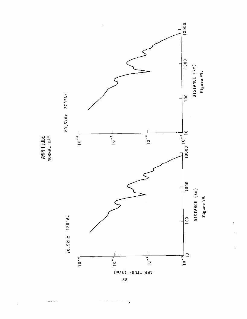
0
0 h cu / N L A ln
0 N I I I
(0
I
0 7
I-
O
N 4 0 0 /
OD
I
0 7
/ co 7
N I Y u) 0 N
I I m 1 W PI
I 0 - I
0 - I 0 -
0 0 7
0 0 0 7
0 0 -
0 - 0 -
h
E Y v
W V L < I- VI U
n
E Y v
W u L 4 I- v, U
n
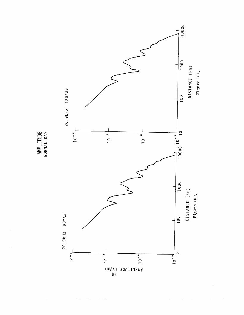
N =c 0 co 0
7
N I Y m 0 N
N =c 0 m 0
N I Y m 0 N
PI I 0 P-
m I 0 7
0 0 0 0 7
0 0 0 7
0 0 7
3 m 7
0 I
7
0 0 0 0 7
0 0 0 7
3 3 -
> -
h
E Y v
W V z U I- v,
0 U
h
E Y v
w V L =c I- v, U
n
4 0
a, k
.-(
?il
iz
0 0
a, k 5 M
4
.r( cr
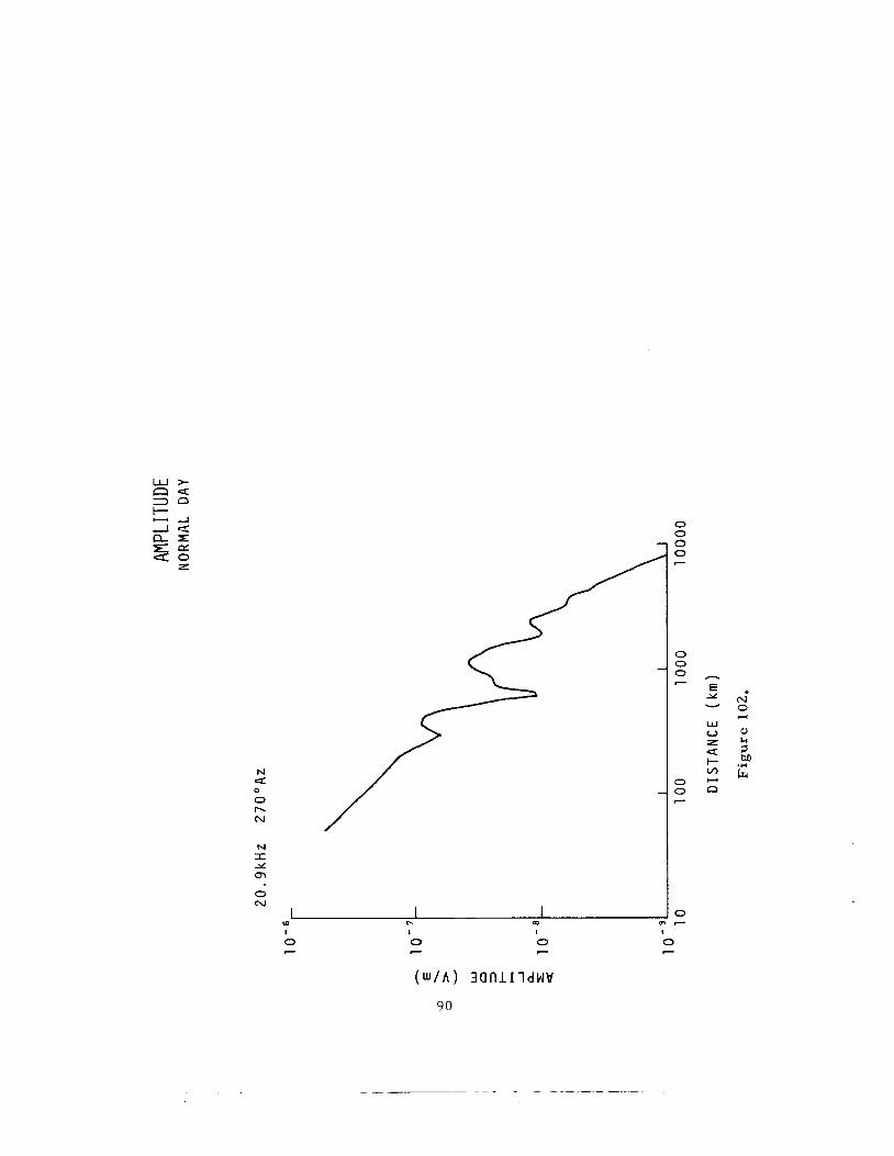
N 5 0 0 h cu
N I Y 0 7
0 c\J
I I I In PI m I I I 0 7
0 c
0 - @ / A ) i a n i ~ i d w v
90
h
E Y v
W V I 5 I- Ln Y
n
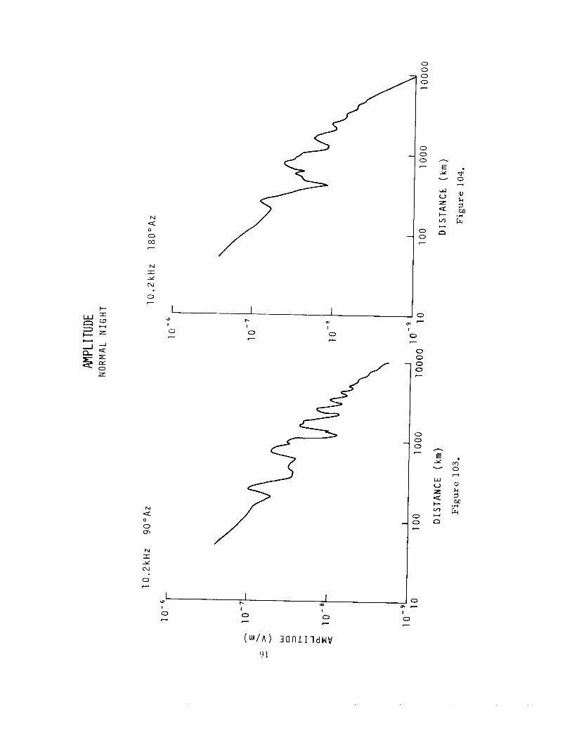
0 0
I- -
z
N
0 0 co P
N X Y N
0 7
N 4 0
0 ol
N I Y N
0 - I I I
m PI 0
I
0 7
0 c
I
0 c
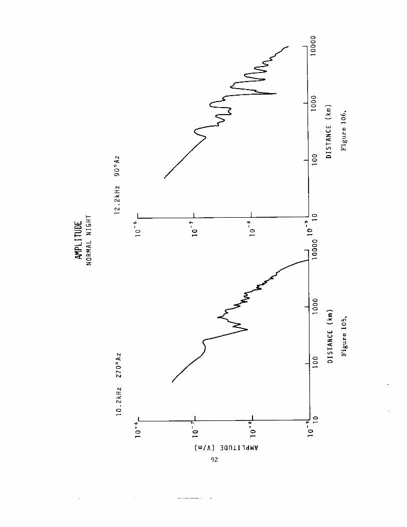
I-
M
N < 0 0 - J
0
N I Y N
cu -
N 4 0 0 h cu
N I Y (u
0 -
I 0 7
I
0 - (D
I
0 F
3 3 -
3 3 3 7
0 0 7
0 m -
0 I
7
- I 0 7
0 7
I 0 c
0 0
0 0 0 0 7
0 0 0 7
0 0 -
0 7
I 0 F
h
E Y v
W V L U I- v,
c3 U
h
E Y v
w V r 4 + v,
0 Y
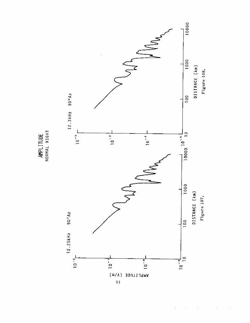
N Q: 0 0 cn
N I Y m N 7
N 4:
0 cn 0
N I Y Ln N
N 7
I I I I
I. m a
0 - 0 - 0 7
I . I I I. (I)
W I 0 - I
0 - I 0 7
0 0 0 0 7
0 0 0 -
0 0 7
3 m -
0 I
7
0 0 0 0 7
0 0 0 7
3 3 -
3 - I 0 -
h
E Y v
W V L 4: I- v, U n
h
E Y v
W V z e I- v, U
n
93
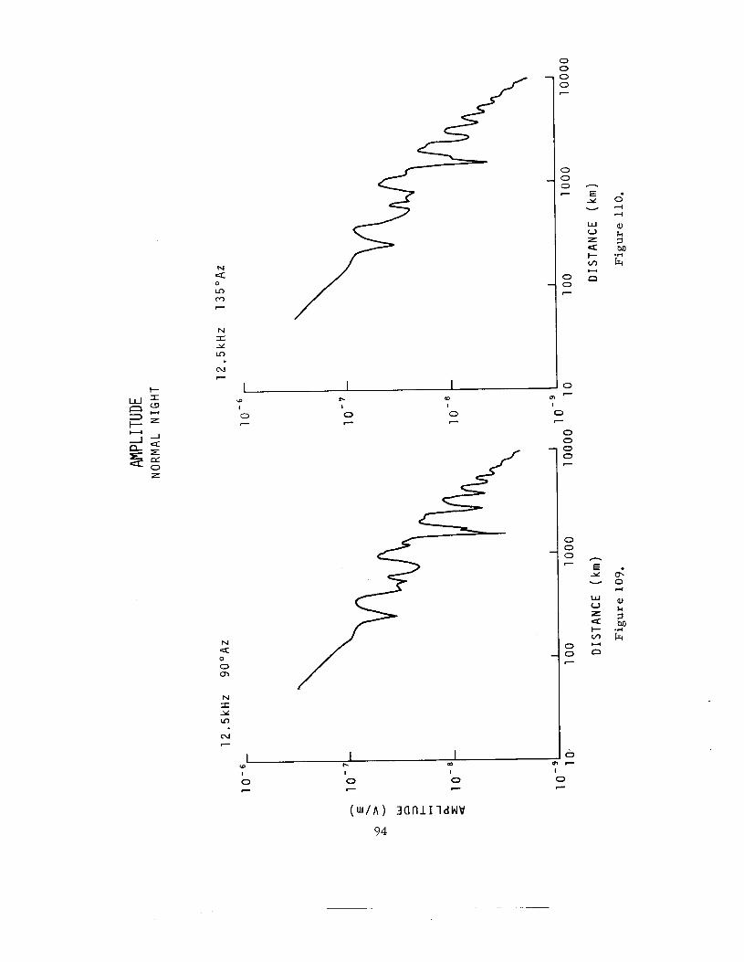
c
z
N Q 0 Lo c-7 - N L A Lo
N e
N 4 0 0 cn
N I Y
0 0 0 0 7
0 0 0 e
0 0 7
I I I l o 0 I
0 c
I. I 0 -
m I
0 -
3 /
1 I m I W r. I 0 c
I 0
I 0 -
m -
0 I
c
0 0 3 3 -
0 0 0 e
0 0 -
0 - 0 -
h
E Y v
w u L 4: I- Ln Y
n
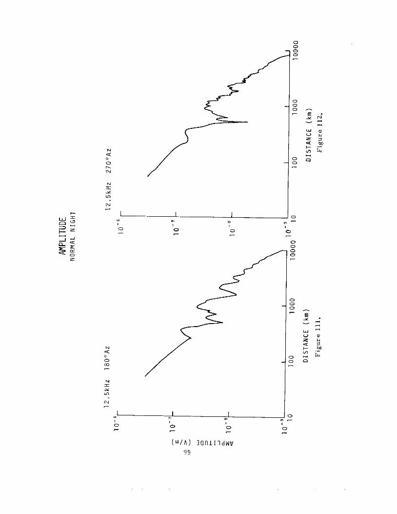
N L Y Lo
N -
0 0 0 0 7
0 0 0 7
3 3 -
I 1 3 (D r.
0 m 7
0 7
I
0 c
/
I
0 -
N L Y Lo
N 7
I I I m (D r.
I
0 7
I
0 c
I
0 7
I
0 7
I
0 7
0 0 0 0 -
0 0 0
0 0 -
3 -
h
E ' Y N
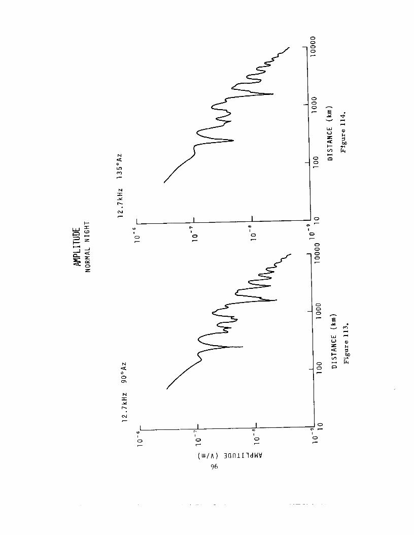
N 4. 0 v) m 7
N L Ai h
N F
N 4 0 0 In
N I Y h
c\I c
I I I I. I
0 - m I 0 - I
0 - 0 0 0 0 -
0 0 0
0 0 7
h
E A v
w V z U I- v) H
n
E Y v
W V L 4 !- m H
n
96
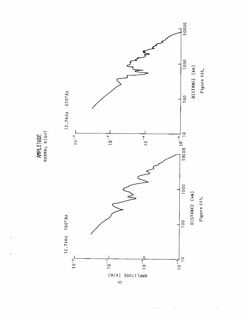
c w = n u 3 - I - = Y
N < 0
0 h N
N L Y h
N 7
N 4:
0 co 0
7
N I Y h
N F
a I 0 7
p. I 0 7
m I 0 7
1 I I l a
l. m W
0 7
0 - 0 7
0 0 0 0 r--
0 0 0 -
0 0 7
3 m -
0 I
7
0 0 c, 0 7
0 0 0 7
3 3 -
3 -
c
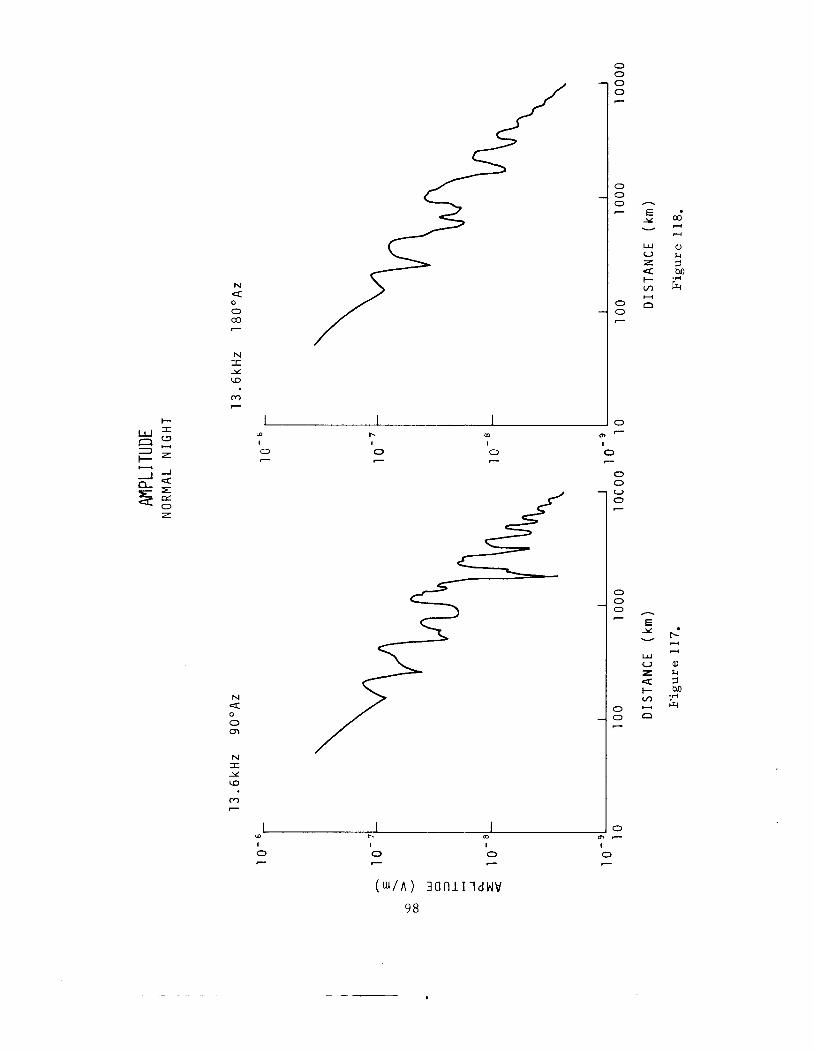
I-
% $ z = Y
I - J
z
N < 0 m 0
7
N I Y u3
m 7
N < 0 cn 0
N I Y u3
m 7
(0
I 0 -
r- I
0 7
0
I 0 7
€
I
0 7
I
0 7
I 0 7
0 0 0 0 7
0 0 0 7
0 0 7
0
1
0 7
n
E Y U
W 0 z 4: I- v,
0 H
n
Y E U
W V z 4: t- v,
13 H
98
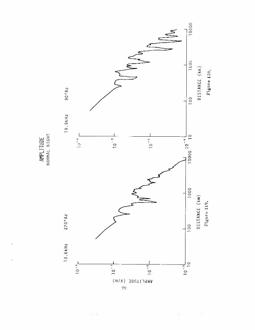
0 0 0 0 ?
0 0 0 7
0 0 I--
3 m e
0 I
7
0 0 0 0 e
0 0 0 7
0 0 7
0 -7
I
0 e
N 4 0 0 cn
N I Y cn cn e
c
ID
I
0 7
.m I
0 7
N CC 0 0 h (u
N I Y u3
m - I I I PI m ID I
0 7
0 7
0 7
99
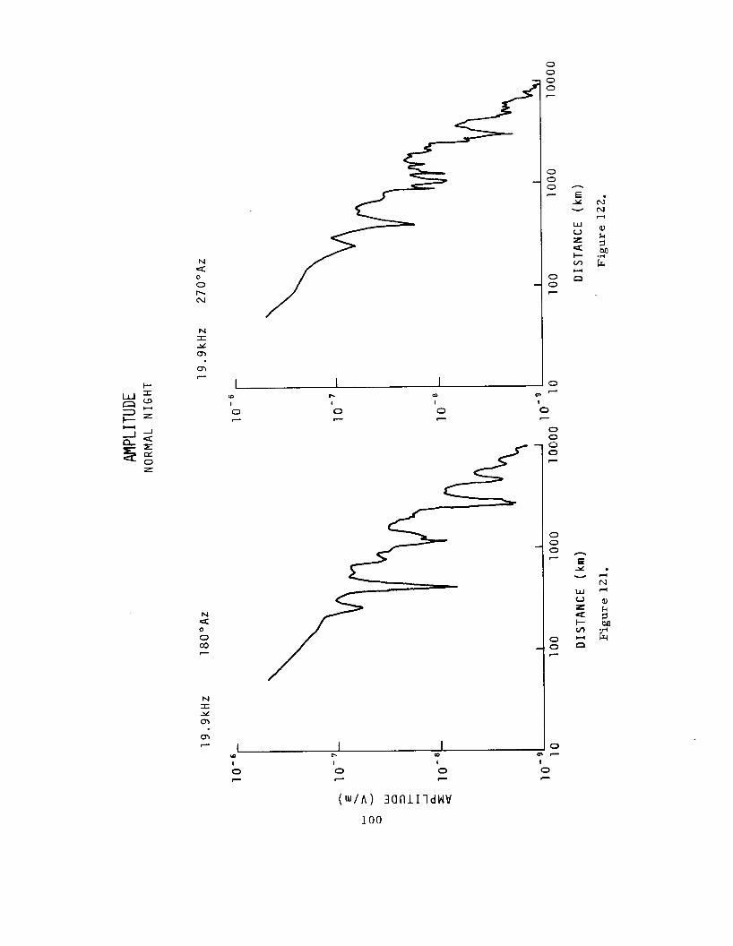
N Q 0 0 h N
N I Y m m 7
a I
0 7
N 4:
0 co 0
c
0-l
0-l 7
PI I
0 c
m I
0 7
N I Y
I 1 I lB PI m
I I I
0 - 0 c
0 c
0 0 0 0 7
0 0 0 c
0 0 7
0
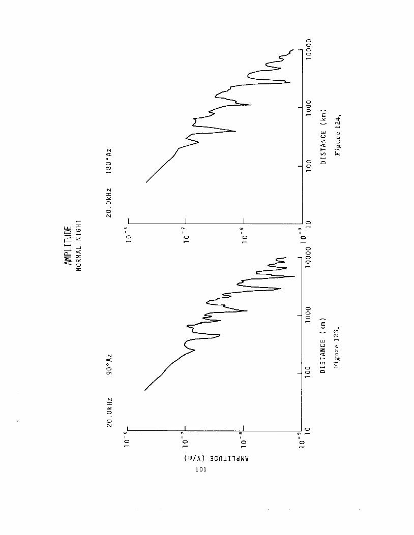
I-
- $ E 2 -
N 4
0 a3
0
- N r Y 0
0 N
N 4 0 0 In
N I Y 0
0 N
(D
I
0 - I. I
0 - m
I
0 c
1 I I a l. m I I I
0 c
0 7
0 7
0 0 0 0 7
0 0 0 7
0 0 -
0 m -
0 I
c
0 0 0 0 7
0 0 0 7
0 0 7
0 - 0 -
h
E Y U
W 0 z 4 t- v,
c3 CI
E Y U
W 0 L =c I- v,
0 -
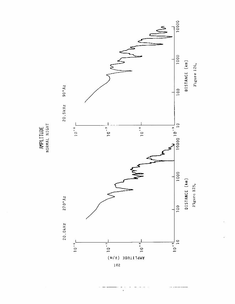
N < 0 0 0-l
N L Y Ln
0 N
/
u. I
0 -
N Q 0 0 h N
N I Y 0
0 N
I 0 7
t. I
0 7
m I
0 7
I 0 - I
0 7
0 0 0 0 7
0 0 0 7
0 0 7
0 m l -
0 I
7
0 0 0 0 ?
0 0 0 l-
0 0 7
0 l-
h
E Y v
W V z < I- m U
n
E Y v
w V L 4 I- m
0 Y
I
0 c
. -
I
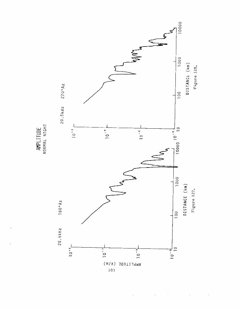
N 4: 0 0 h N
N I Y Ln
0 N
I-
0 0
0 7
0 -
N 4:
0 co 0
7
I
0 P
N I Y Ln
0 N I I I
m r. (D
I 0 P
0 0 0 0 ?
3L
0 0 0 ?
3 3 -
3 -
h
E Y v
W V z I- m c(
n
h
E Y v
w V z < I- v,
0 U
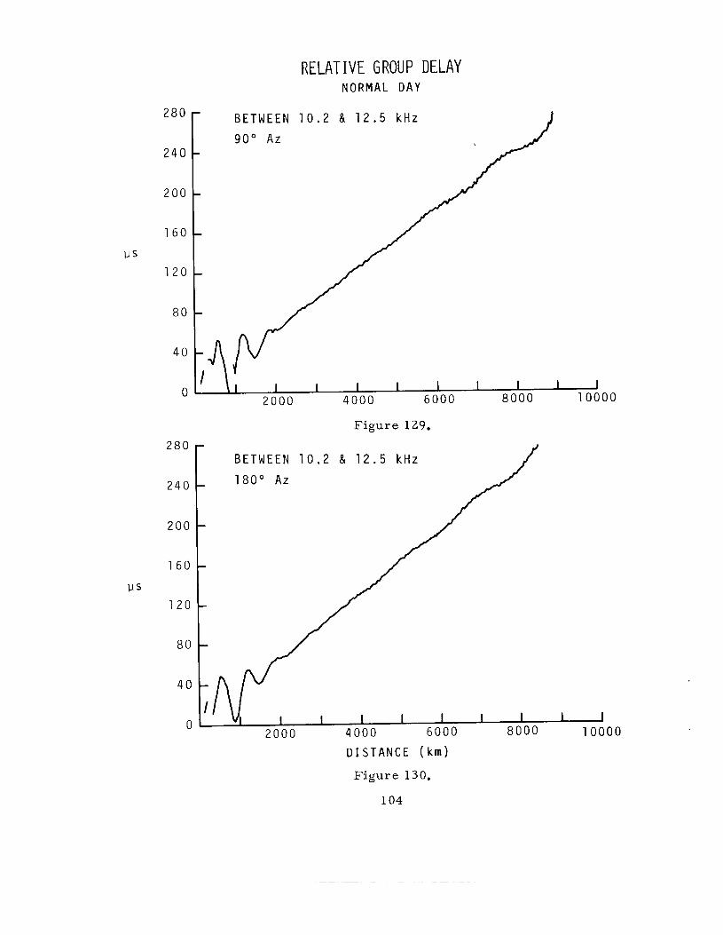
RELATIVE GROUP DELAY N O R M A L D A Y
BETWEEN 1 0 . 2 & 1 2 . 5 kHz J 90" A z
280 1
2 4 0
2 0 0
1 6 0
1 2 0
8 0
4 0
0
F i g u r e 129.
BETWEEN 1 0 . 2 & 1 2 . 5 k H z
1 8 0 " Az
-
- I I I
2 0 0 0 4 0 0 0 6 0 0 0 8 0 0 0 1 0 0 0 0
D I S T A N C E ( k m )
F i g u r e 130.
104
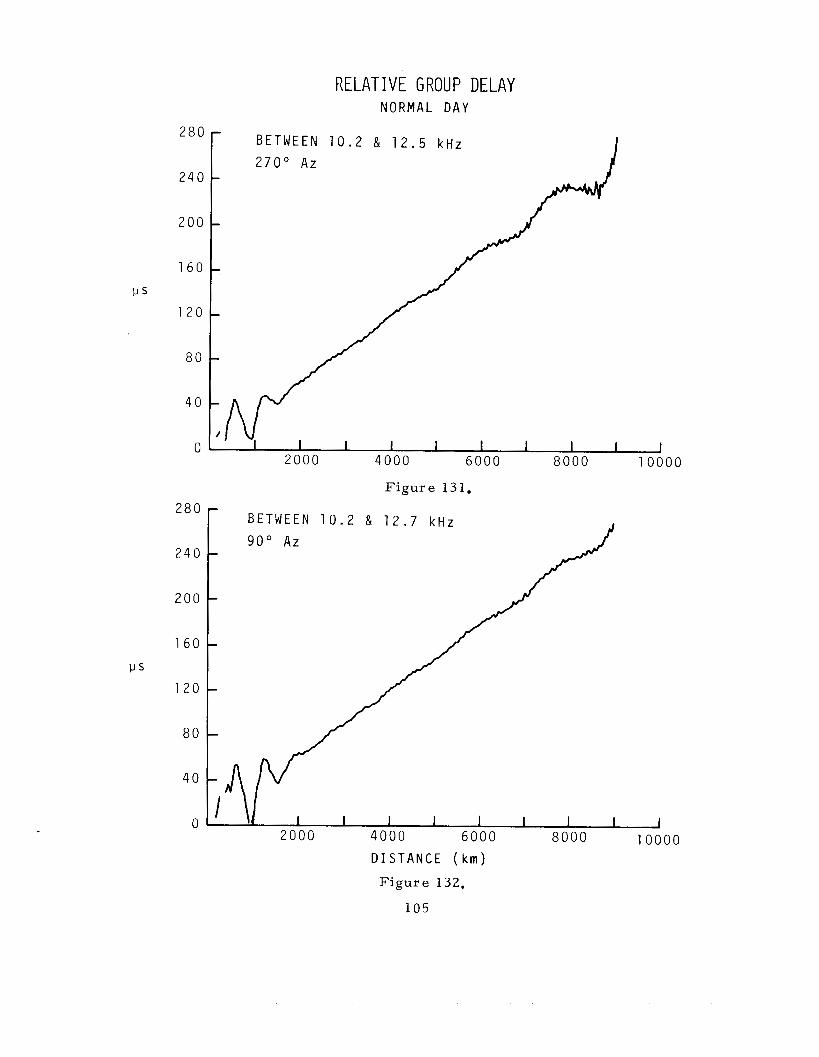
RELATIVE GROUP DELAY NORMAL D A Y
28C
24C
200
1 6 0
U s 1 2 0
80
40
0
280
240
200
1 6 0
us 120
80
40
0
BETWEEN 10.2 & 12.5 kHz 270" Az
BETWEEN 1 0 . 2 & 12.7 kHz 9 0 " Az
2000 4000 6000 8000 10000
F i g u r e 131.
1 1 0 0 0 0
D I S T A N C E ( k m )
F i g u r e 132.
1 0 5
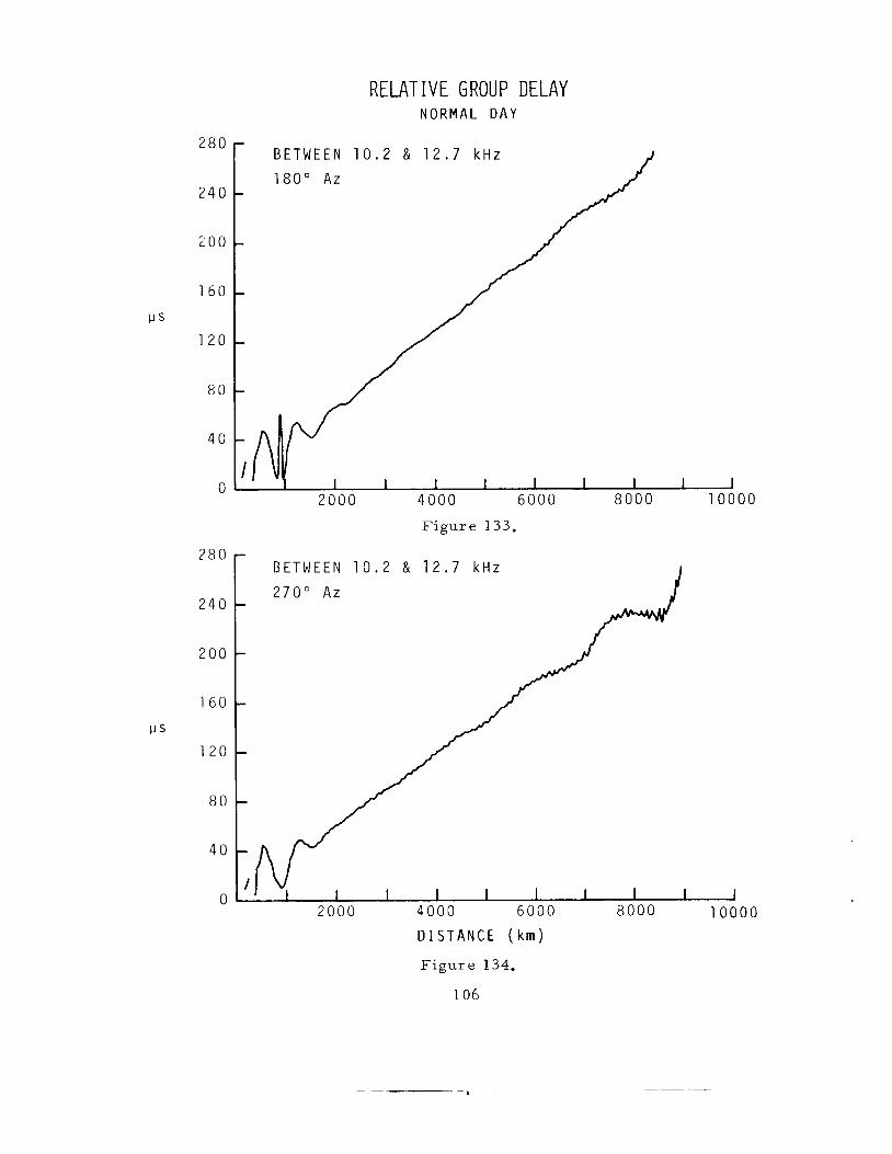
RELATIVE GROUP DELAY N O R M A L D A Y
2 8 0
2 4 0
2 0 0
1 6 0
P S
1 2 0
8 0
4 0
0
2 8 0
2 4 0
2 0 0
1 6 0
1 2 0
8 0
4 0
0
B E T W E E N 1 0 . 2 1 8 0 " Az
I 1 I I I I 1 1
2 0 0 0 4 0 0 0 6 0 0 0 8 0 0 0 1 0 0 0 0
F i g u r e 133.
- BETWEEN 1 0 . 2 & 1 2 . 7 k H z
2 7 0 " Az -
-
-
-
-
- I
I 1 2 0 0 0 4 0 0 0 6 0 0 0 8 0 0 0 1 0 0 0
- BETWEEN 1 0 . 2 & 1 2 . 7 k H z
2 7 0 " Az -
-
-
-
-
- I
I 1 2 0 0 0 4 0 0 0 6 0 0 0 8 0 0 0 1 0 0 0 0
D I S T A N C E ( k i n )
F i g u r e 134.
106
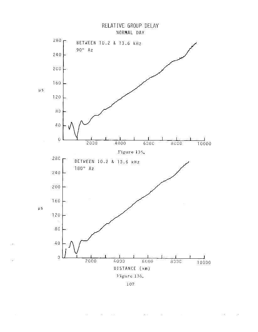
RELATIVE GROUP DELAY N O R M A L D A Y
280
240
200
1 6 0
1 2 0
80
40
0
280
240
200
1 6 0
1-1s
1 2 0
80
40
0
I- B E T W E E N 1 0 . 2 & 1 3 . 6 k H z
90" Az
-
2000 4000 6000 8000 10000 1
if
B E T W E E N 1 0 . 2 & 1 3 . 6 k H z r 1 8 0 " Az
I 1 I I 2000 4000
1 10000
F i g u r e 135.
00 D I S T A N C E ( k m )
F i g u r e 136.
1 0 7
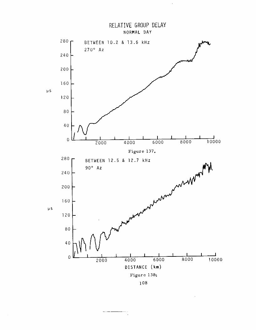
RELATIVE GROUP DELAY NORMAL D A Y
2 8 0
2 4 0
2 0 0
1 6 0
1 2 0
8 0
4 0
0
B E T W E E N 1 0 . 2 & 1 3 . 6 kHz r 2 7 0 " Az
2 8 0
2 4 0
2 0 0
1 6 0
1 2 0
8 0
4 0
0
i I I I 1 I I I I I J 2 0 0 0 4 0 0 0 6 0 0 0 8 0 0 0 1 0 0 0 0
F i g u r e 137.
B E T W E E N 1 2 . 5 & 1 2 . 7 kHz
9 0 " Az
2 8 0 -
2 4 0 -
2 0 0 -
1 6 0 -
1 2 0 -
2 0 0 0 4 0 0 0 6000 8 0 0 0 1 0 0 0 0 J 000
D I S T A N C E ( k m )
F i g u r e 138;
108
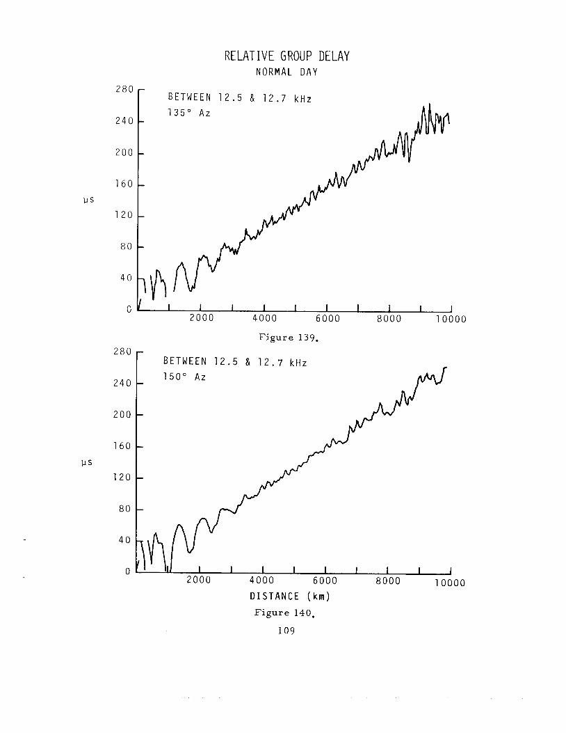
RELATIVE GROUP DELAY NORMAL D A Y
u s
280
240
200
1 6 0
120
80
40
0
r BETWEEN 1 2 . 5 & 1 2 . 7 k H z 1 3 5 " Az
U I 1 I 1 I 1 1 I I 1 2000 4000 6000 8000 10000
F i g u r e 139,
280 - BETWEEN 1 2 . 5 & 12.7 k H z 1 5 0 " Az 240 -
200 -
1 6 0 -
120 - 8 0 -
2000 4000 6000 8000 10000 D I S T A N C E ( k m )
F i g u r e 140,
109
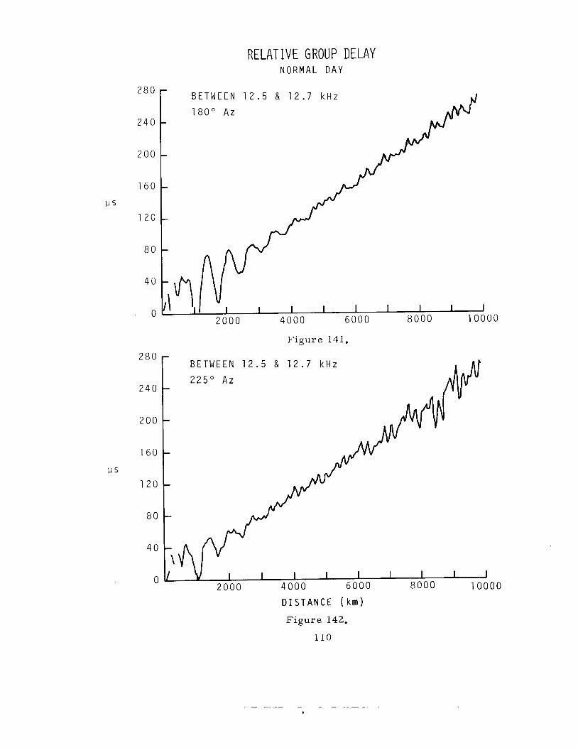
RELATIVE GROUP DELAY N O R M A L D A Y
2 8 0
2 4 0
200
1 6 0
1 2 0
8 0
40
0 h
B E T W E E N 1 2 . 5 & 1 2 . 7 k H z
1 8 0 " Az
I 2 0 0 0 4 0 0 0 6 0 0 0 8 0 0 0 1 0 0 0
I 1 I I I I I I 2 0 0 0 4 0 0 0 6 0 0 0 8 0 0 0 1 0 0 0
I ' I
F i g u r e 141.
0
u s
D I S T A N C E ( k m )
F i g u r e 142.
110
,
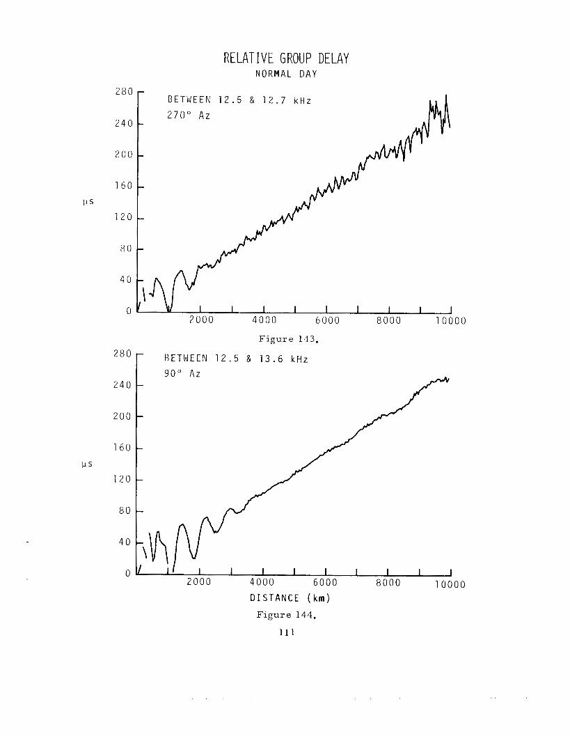
40
0
280
240
200
1 6 0
lis
120
80
40
0
RELATIVE GROUP DELAY N O R M A L D A Y
B E T W E E N
2 7 0 " A z
V I I I I I 1 I I J 2000 4000 6 0 0 0 8000 10000
F i g u r e 143.
- B E T W E E N 1 2 . 5 & 1 3 . 6 k H z
90" A z -
I ; / 1 I 1 1 I I 1 1 1 4 0 0 0 6 0 0 0 8 0 0 0 1 0 0 0 0 2000 D I S T A N C E ( k m )
Figure 144.
111
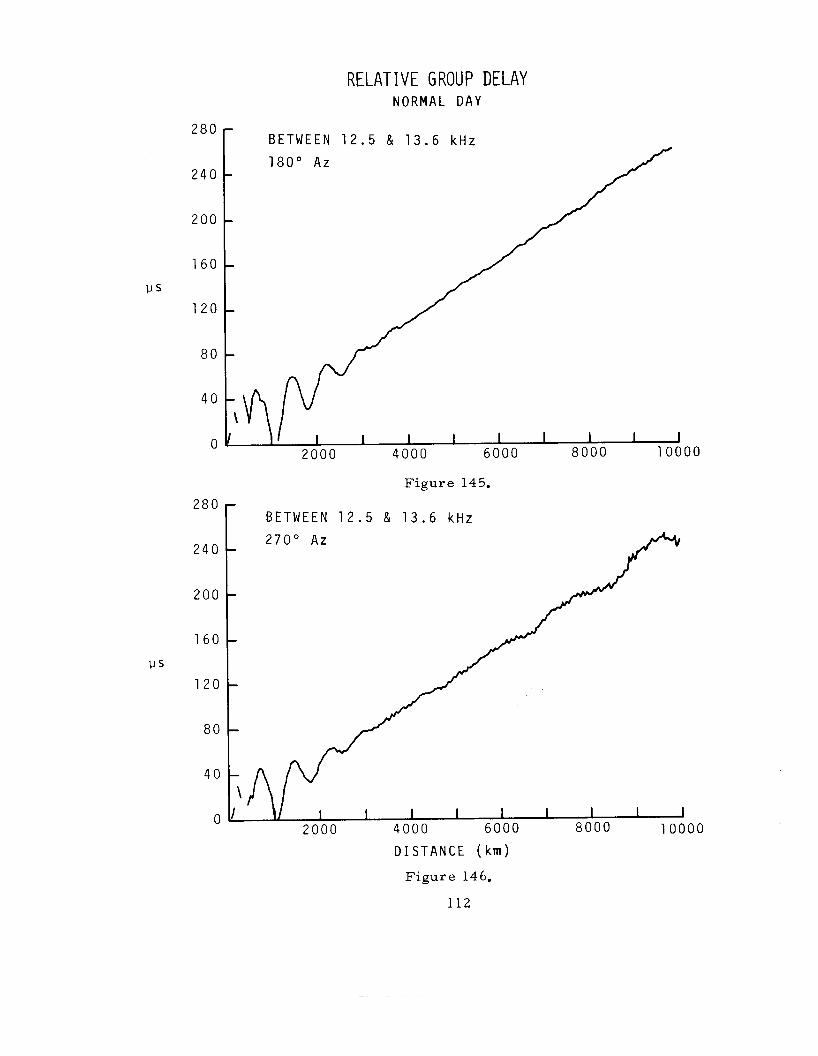
RELATIVE GROUP DELAY NORMAL D A Y
2 8 0
2 4 0
2 0 0
1 6 0
1 2 0
8 0
4 0
0
2 8 0
2 4 0
2 0 0
1 6 0
1 2 0
8 0
4 0
0
c
BETWEEN 1 2 . 5 & 1 3 . 6 k H z
1 8 0 " Az
\ J 1
2 0 0 0 4 0 0 0 6 0 0 0 8 0 0 0 1 0 0
F i g u r e 145.
00
- BETWEEN 1 2 . 5 & 1 3 . 6 k H z
2 7 0 " A z
\ I I
2 0 0 0 4 0 0 0 6 0 0 0 8 0 0 0 1 0 0 0
r BETWEEN 1 2 . 5 & 1 3 . 6 k H z
0
DISTANCE ( k m )
F i g u r e 146.
112
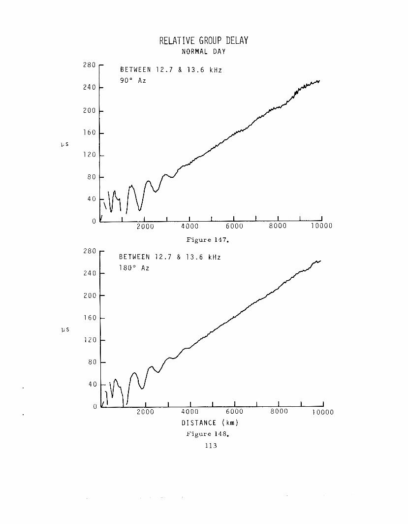
us
RELATIVE GROUP DELAY N O R M A L D A Y 280r BETWEEN 12.7 & 1 3 . 6 kHz
240
200
160
120
8 0
40
0
280
240
2 0 0
1 6 0
1 2 0
8 0
40
0
Figure 147.
BETWEEN 12.7 & 1 3 . 6 k H z 1 8 0 " A z
I I 1 I 1 I 1 1 1 2 0 0 0 4000 6 0 0 0 8 0 0 0 1 0 0 0
D I S T A N C E ( k m ) Figure 148.
113
0
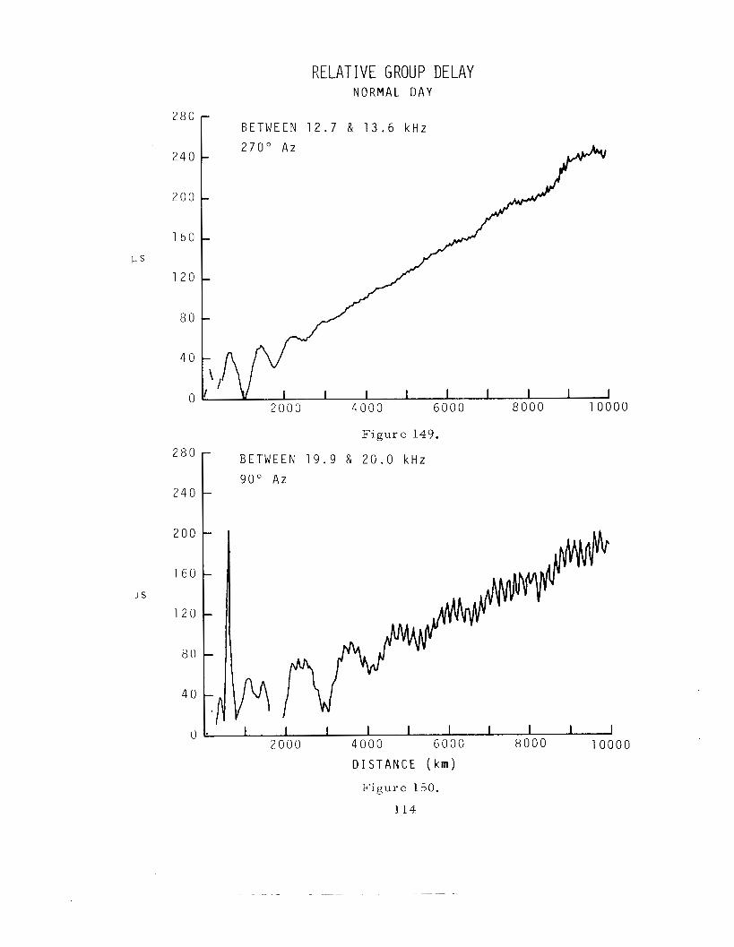
RELATIVE GROUP DELAY N O R M A L D A Y
1s
" O r BETWEEN 1 2 . 7 & 1 3 . 6 k H z
240
200
160
120
80
40
0 2000 4000 6000 8000 1 0 0 0 0
F i g u r e 149.
BETWEEN 1 9 . 9 & 2 0 . 0 k H z
280 r A z
240 t 200
160
120
80
40
0 1. 1 I I I 1 1 I I 1 1 2000 4000 6000 8000 10000
D I S T A N C E ( k m )
F i g u r e 150.
114
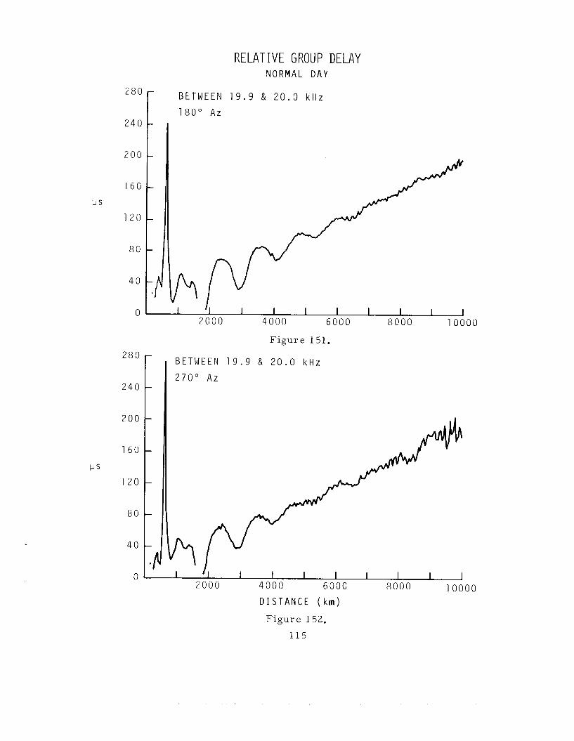
280
240
200
1 6 0
120
80
40
0
RELATIVE GROUP DELAY N O R M A L D A Y
B E T W E E N 1 9 . 9 & 2 0 . 0 k H z
180" A z
280
240
200
1 6 0
us 120
80
40
0
F i g u r e 151. -
B E T W E E N 1 9 . 9 & 2 0 . 0 k H z 1 2 7 0 " A z
I I I I I I I 1 6000 8000 1000
I , 2000 4000
D I S T A N C E ( k m )
F i g u r e 152.
1 1 5
0
0

RELATIVE GROUP DELAY NORMAL D A Y
BETWEEN 1 9 . 9 & 2 0 . 5 kHz
9 0 " Az 240
200
1 6 0
120
8 0
40
0
1
0
F i g u r e 153.
BETWEEN 1 9 . 9 & 2 0 . 5 kHz
280 r . 1k3O Az 240
200
1 6 0
120
80
40
n 4 0 0 0
v -
2000 0 D I S T A N C E ( k m )
F i g u r e 154.
116

RELATIVE GROUP DELAY N O R M A L D A Y
280 r B E T W E E N 1 9 . 9 & 2 0 . 5 kHz
1 6 0
1 2 0
80
40
0
F i g u r e 155.
B E T W E E N 1 9 . 9 & 2 0 . 9 k H z
280 c A z
1 6 0
1 2 0
8 0
40
0
D I S T A N C E ( k m )
F i g u r e 156.
117

U S
200
1 6 0
120
80
40
RELATIVE GROUP DELAY N O R M A L D A Y
-
-
-
-
-
B E T W E E N 1 9 . 9 & 2 0 . 9 kHz 1 8 0 " Az
240
I I I I I 1 I 1 I I 1 0 0 0 0 0 1 2000 4000 6 0 0 0 8000
F i g u r e 157.
280 r BETWEEN 1 9 . 9 & 2 0 . 9 k H z
2 4 0
200
1 6 0
120
8 0
40
0
D I S T A N C E ( k m )
F i g u r e 158.
118
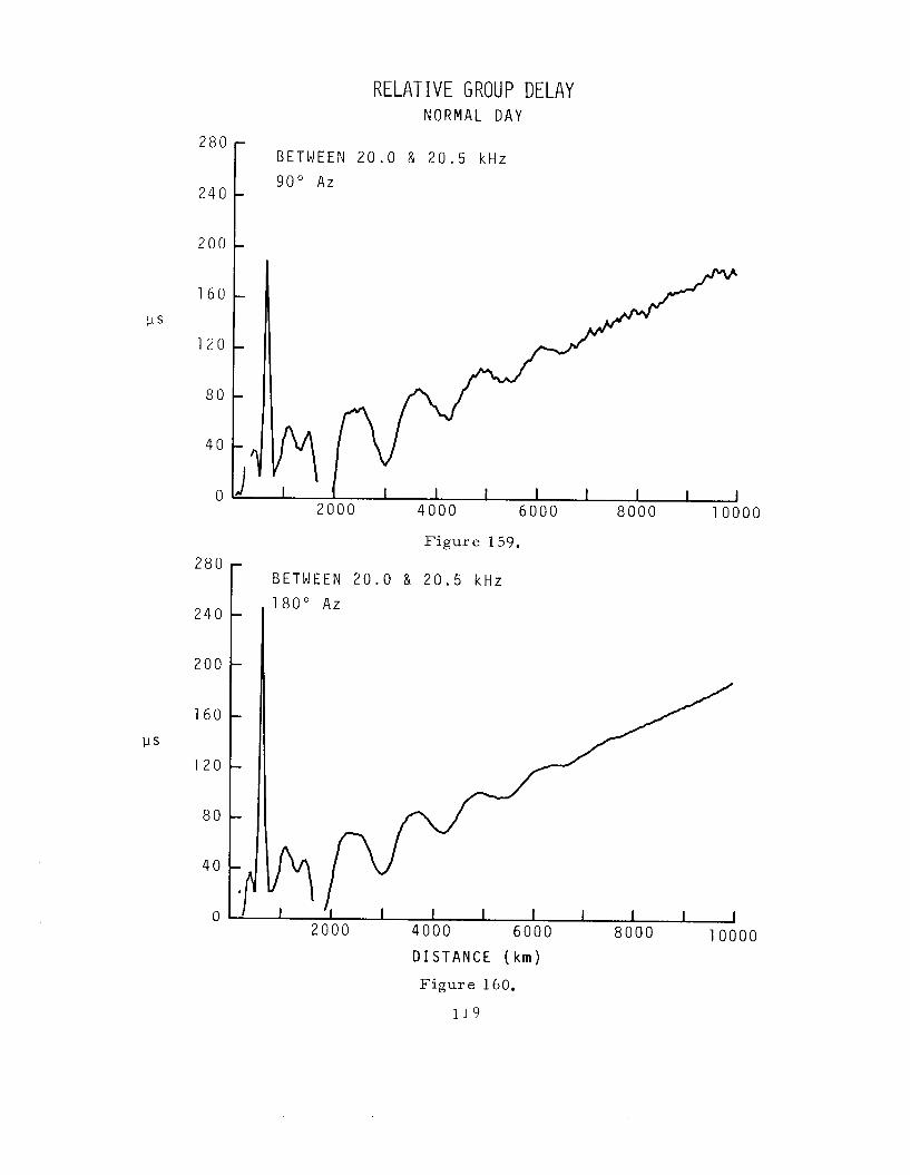
RELATIVE GROUP DELAY N O R M A L D A Y
B E T W E E N 2 0 . 0 & 2 0 . 5 kHz
90" Az
200
1 6 0
120
80
40
0
2 8 0
240
200
1 6 0
1 2 0
8 0
40
0
2
F i g u r e 159.
B E T W E E N 2 0 . 0 & 2 0 . 5 kHz
, 1 8 0 " Az
2000 4000 6000 D I S T A N C E ( k m )
F i g u r e 160.
119
0
8000 1 0 0 0 0
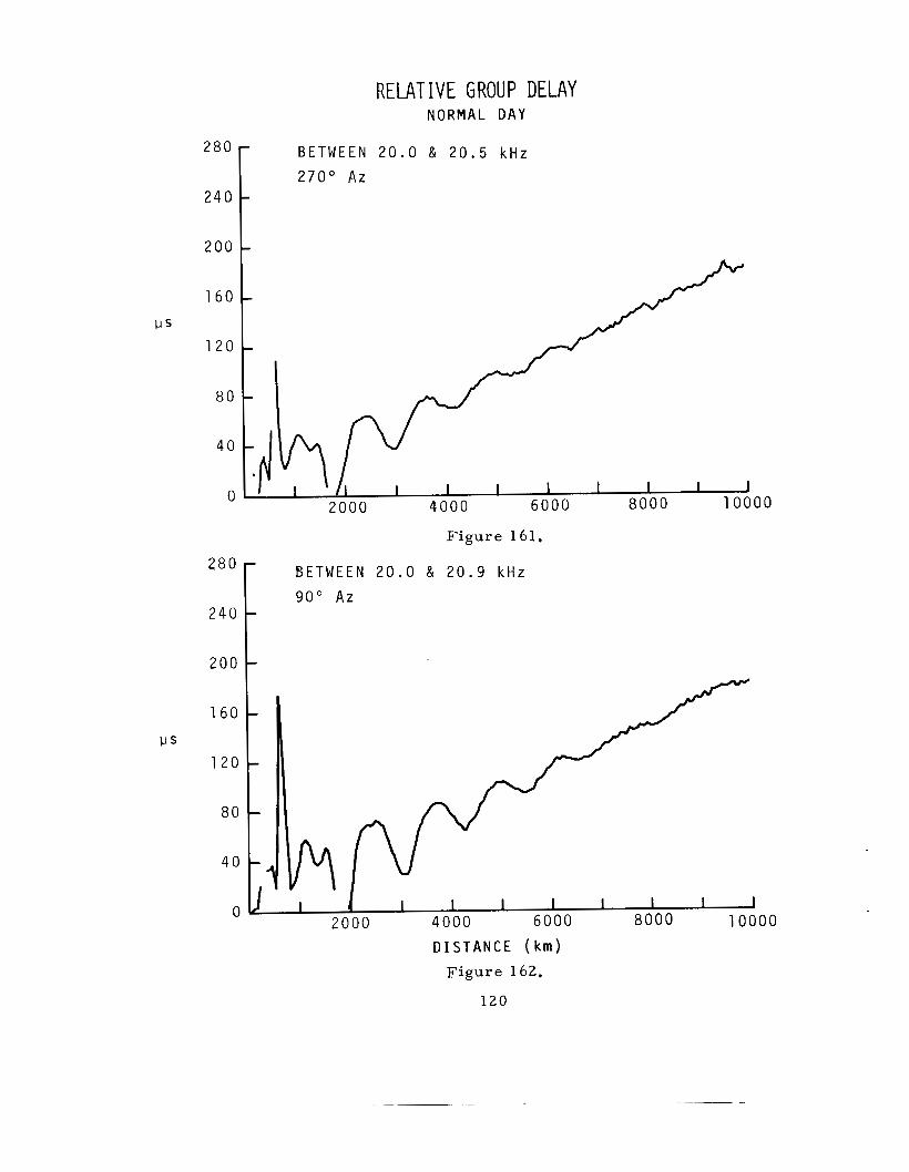
280
2 0 0
RELATIVE GROUP DELAY N O R M A L D A Y
B E T W E E N 20.0 & 20.5 k H z
2 7 0 " A z
1 6 0 - F.rs
1 2 0 -
2 0 0 0 4 0 0 0 6 0 0 0 8 0 0 0 1 0 0 0 0 0
F i g u r e 161. 280r B E T W E E N 20.0 & 20.9 k H z
9 0 " Az 2 4 0
2 0 0
1 6 0
1 2 0
8 0
4 0
0 L 6 0 0 0 8000
I 1 0 0 0 0
D I S T A N C E ( k m ) F i g u r e 162.
120
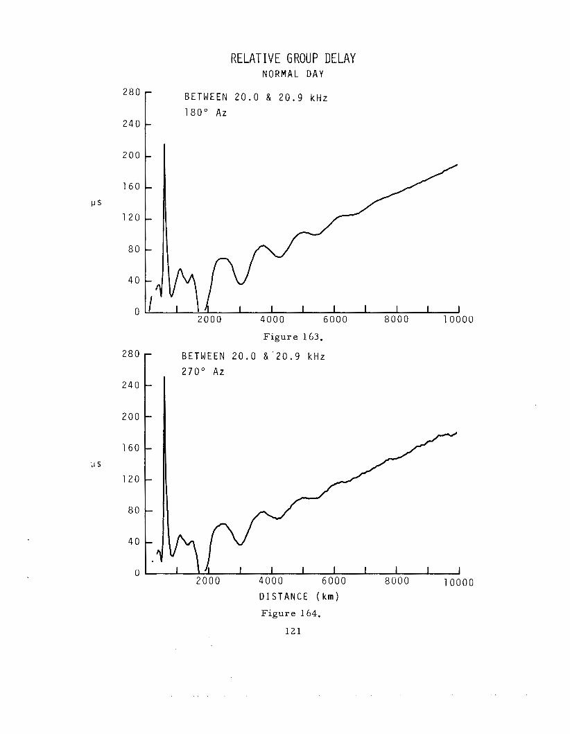
lJs
RELATIVE GROUP DELAY N O R M A L D A Y
BETWEEN 2 0 . 0 & 2 0 . 9 kHz
1 8 0 " Az 2 4 0 2 a o F 2 0 0
1 6 0
1 2 0
a 0
40
0
280
2 4 0
200
1 6 0
1 2 0
a 0
40
0
Figure 163.
BETWEEN 2 0 . 0 t i ' 2 0 . 9 k H z r 2 7 0 " A z -
-
-
-
- -
4
I I I I 1 I I I 4000 6000 8000 1 0 0 0 0 2 0 0 0 DISTANCE ( k m )
Figure 164.
121
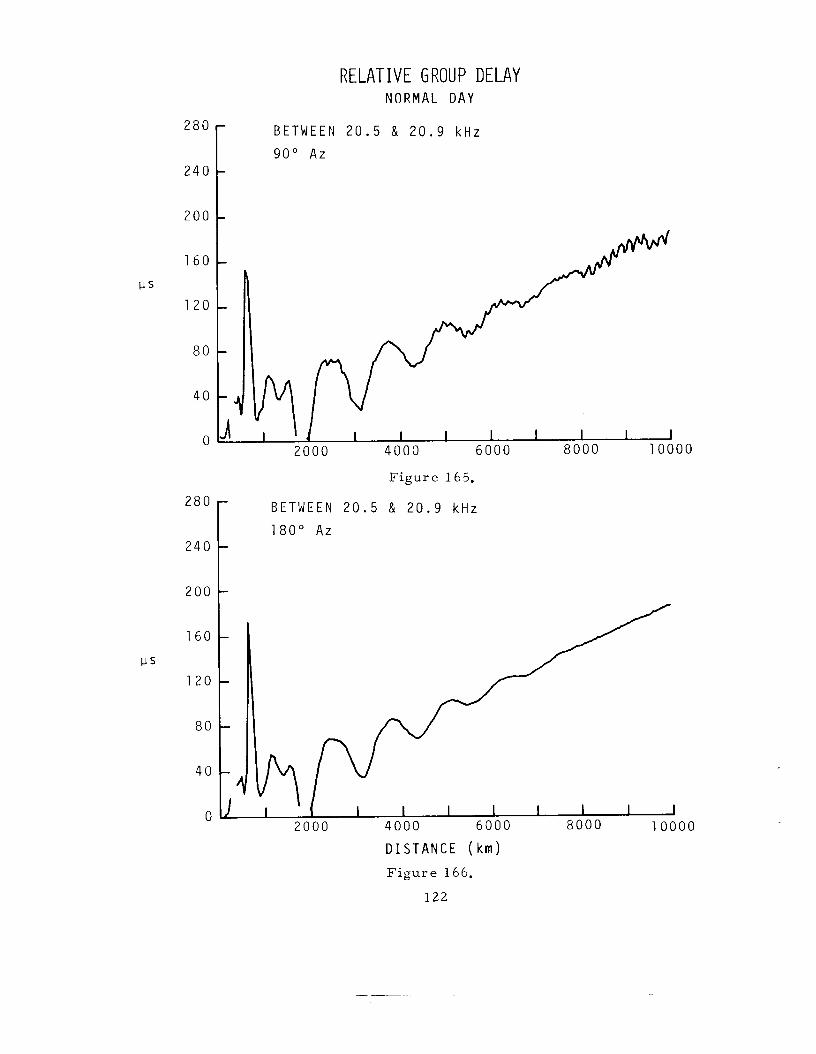
RELATIVE GROUP DELAY N O R M A L D A Y
-
-
BETWEEN 2 0 . 5 & 2 0 . 9 kHz
9 0 " Az 2 8 0 r 240
200
1 6 0
1 2 0
8 0
4 0
0
2 8 0
2 4 0
2 0 0
1 6 0
1 2 0
8 0
40
0
F i g u r e 165.
BETWEEN 2 0 . 5 & 2 0 . 9 kHz
1 8 0 " Az
0
D I S T A N C E ( k m )
F i g u r e 166.
1 2 2
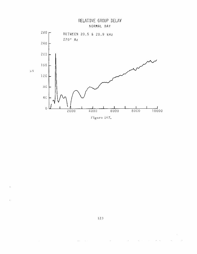
RELATIVE GROUP DELAY N O R M A L D A Y
B E T W E E N 2 0 . 5 & 20.9 k H z 2 7 0 " A z
240
200
1 b o
D S
1 2 0
80
40
0
Figure 167.
0 0
1 2 3
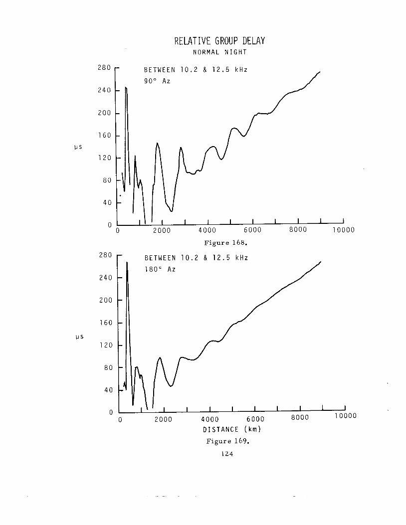
2 8 0
2 4 0
2 0 0
1 6 0
1 2 0
80
40
0
RELATIVE GROUP DELAY NORMAL N I G H T
B E T W E E N 1 0 . 2 & 1 2 . 5 kHz
2 8 0
2 4 0
2 0 0
1 6 0
1 2 0
8 0
40
0
I I I I
0 2 0 0 0 4 0 0 0 6 0 0 0
I . 1 , I
8 0 0 0 1 0 0
F i g u r e 168.
r B E T W E E N 1 0 . 2 & 1 2 . 5 k H z
00
I 1 I ' I I 1
0 2 0 0 0 4 0 0 0 6 0 0 0 I I I I
8000 1 0 0 0
D I S T A N C E ( k m )
F i g u r e 169.
1 2 4
0
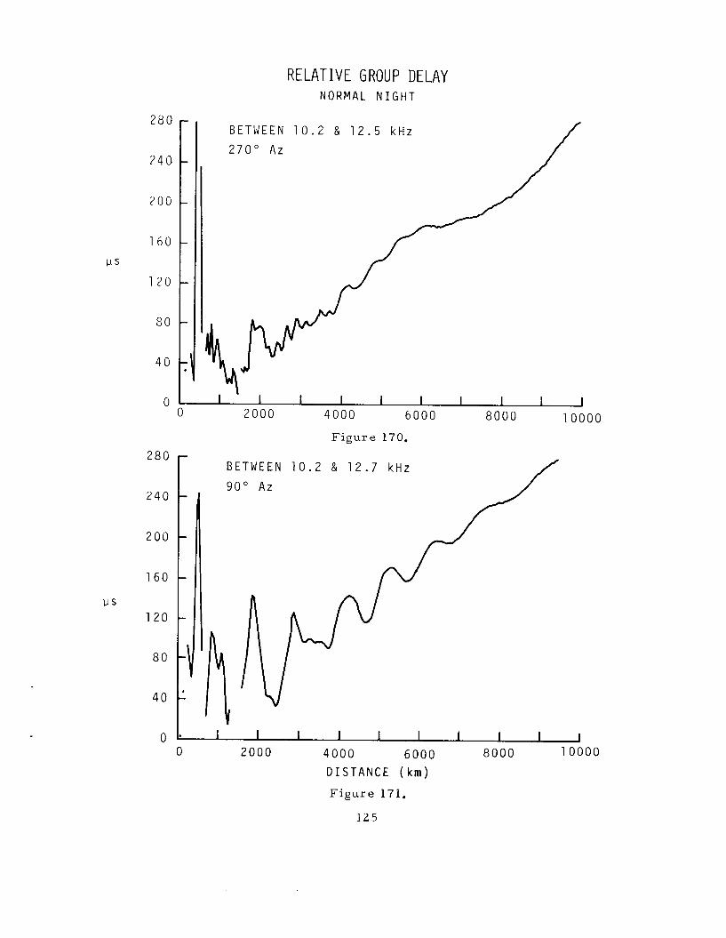
u s
280
2 4 0
200
1 6 0
1 2 0
80
40
280
240
200
1 6 0
1 2 0
80
40
0
-
-
-
-
-
-
RELATIVE GROUP DELAY N O R M A L N I G H T
B E T W E E N 1 0 . 2 & 1 2 . 5 k H z [ I 2 7 0 " Az
0 1. I I I I I I 1 I I I
/
I 1 I I
0 2000 4000 6 0 0 0 8000 Figure 170.
1 0 0 00
1 2 5
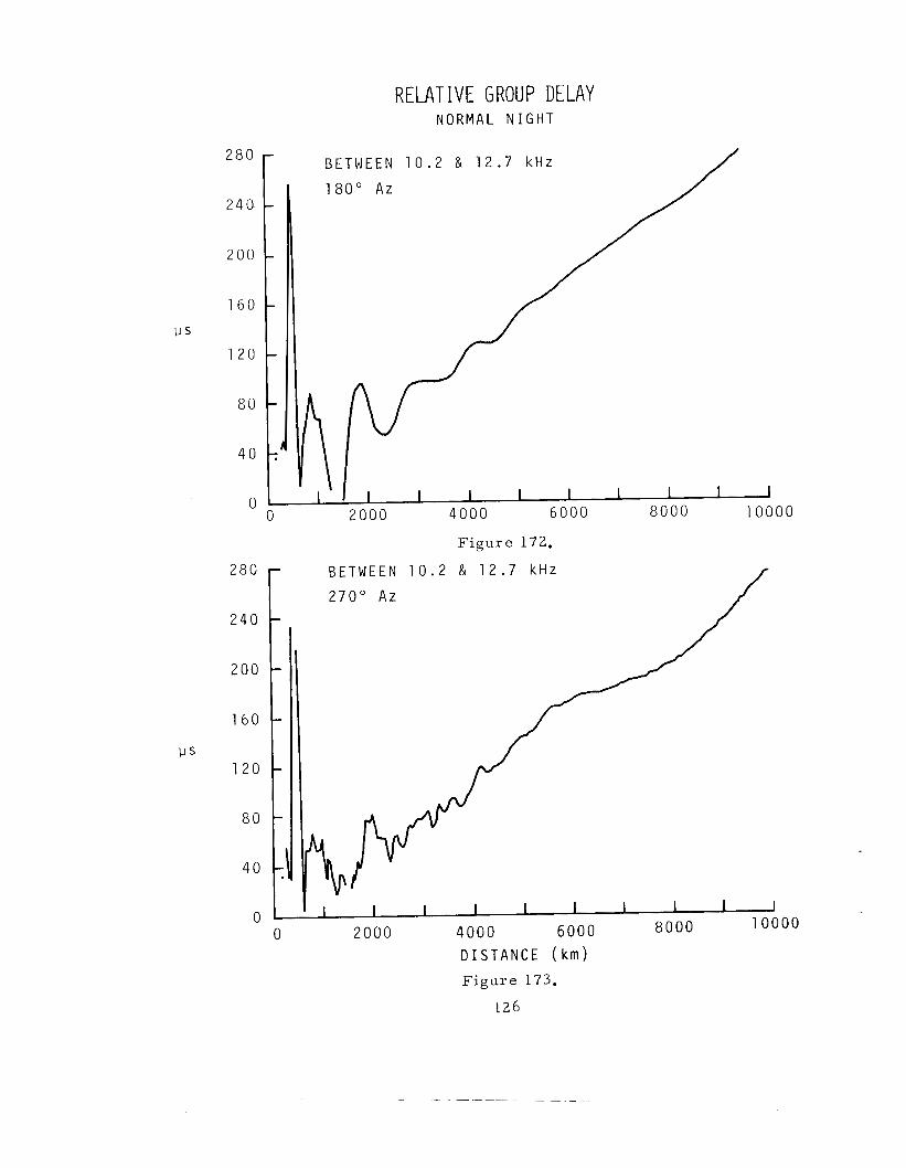
120
40
280 r 240
200
1 6 0
120
80
40
0
RELATIVE GROUP DELAY N O R M A L N I G H T
0
F i g u r e 172.
B E T W E E N 10.2 & 1 2 . 7 kHz
2 7 0 " A z
F i g u r e 172.
B E T W E E N 10.2 & 1 2 . 7 kHz
2 7 0 " A z
D I S T A N C E ( k m ) F i g u r e 173.
126
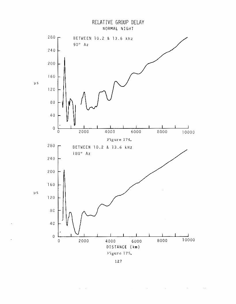
280
240 1
RELATIVE GROUP DELAY N O R M A L N I G H T
0
Figure 174.
B E T W E E N 1 0 . 2 & 1 3 . 6 k H z
200
1 6 0
1 2 0
8 0
40
0 0 2000 4000 6 0 0 0 8 0 0 0 1 0 0 0 0
D I S T A N C E ( k m ) F i g u r e 175.
127
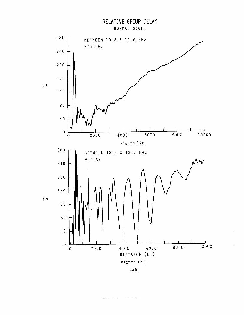
2 8 0
2 4 0
2 0 0
1 6 0
1 2 0
8 0
40
0
2 8 0
2 4 0
2 0 0
1 6 0
1 2 0
8 0
40
0
RELATIVE GROUP DELAY NORMAL N I G H T
/- B E T W E E N 1 0 . 2 & 13.6 kHz r 2 7 0 " Az
I I I I I
0 2 0 0 0 4 0 0 0 6 0 0 0 I 1
Figure 176.
B E T W E E N 1 2 . 5 & 1 2 . 7 kHz
8 0 0 0 1 0 0 0 0
I I I I I I I 1 I
8 0 0 0 1 0 0 0 2 0 0 0 4 0 0 0 6 0 0 0 D I S T A N C E ( k m )
Figure 17'7.
1 2 8
0 0
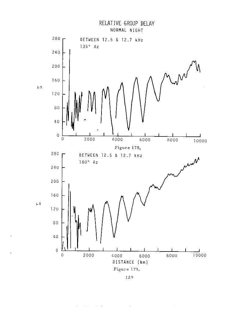
RELATIVE GROUP DELAY N O R M A L NIGHT
BETWEEN 12.5 & 12.7 kHz
240
200
1 6 0
1 2 0
80
40
n
280
240
200
1 6 0
P S 120
8 0
40
0
- -
-
-
-
-
-
L
00 Figure 178.
BETWEEN 12.5 & 12.7 kHz 1 8 0 " A z
I ' 1 I I I 1 I I I 1 0 0 0 0 2000 4000 6000 8000
D I S T A N C E ( k m ) Figure 179.
129
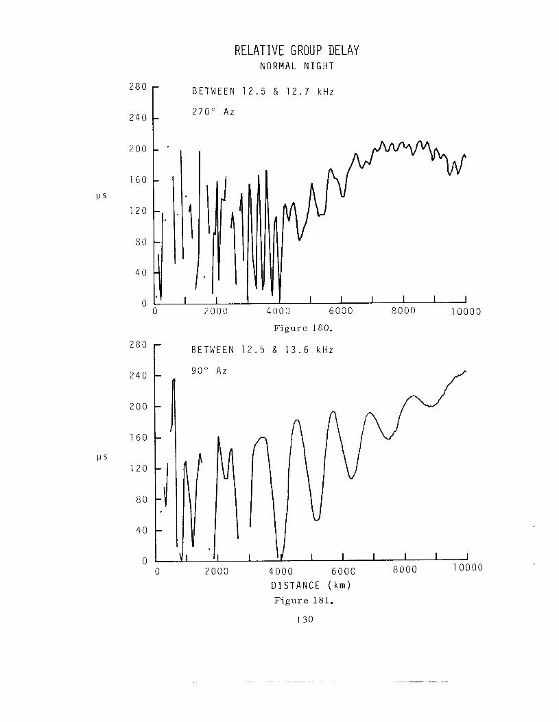
RELATIVE GROUP DELAY N O R M A L N I G H T
280
240
200
1 6 0
I-IS
120
80
40
0
u s
280
240
200
1 6 0
120
80
40
0
B E T W E E N 1 2 . 5 & 1 2 . 7 k H z
2 7 0 " A z
.I\ I I I I I I I I 1
I
I 2000 4000 6000 8000 100 I 2000 4000 6000 8000 100 F i g u r e 180.
B E T W E E N 1 2 . 5 8 1 3 . 6 k H z r 00
D I S T A N C E ( k m ) F i g u r e 181.
130
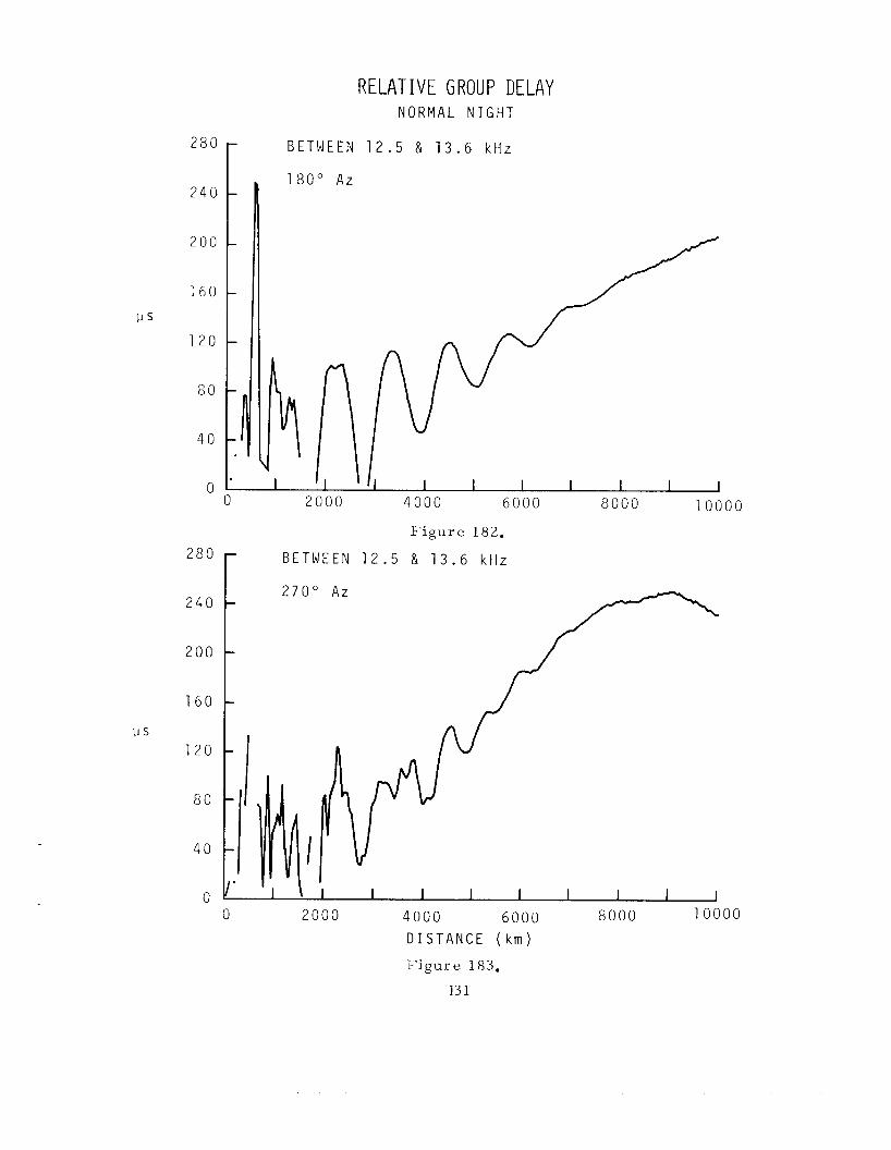
RELATIVE GROUP DELAY N O R M A L NIGHT
u s
B E T W E E N 12.5 & 13.6 kHz 280 r 240
200
160
120
80
40
0 U
F i g u r e 182.
B E T W E E N 12.5 & 13.6 kHz
00
270" Az
0 0 2000 4000 6000 8000 10000
DISTANCE ( k m )
F i g u r e 183.
13 1
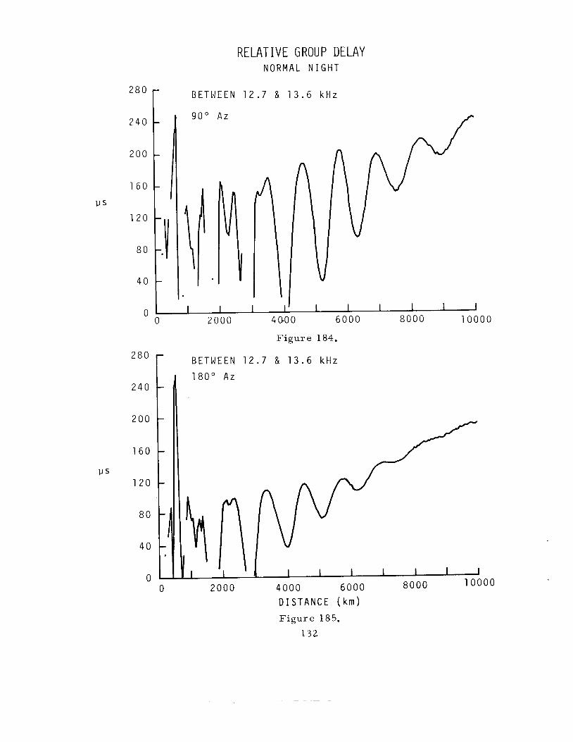
RELATIVE GROUP DELAY N O R M A L N I G H T
- BETWEEN 1 2 . 7 & 1 3 . 6 k H z
9 0 " A 2 -
-
-
I 2 0 0 0 4 0 0 0 6 0 0 0 8 0 0 0 1 0 0
:l'l.l I I I I , I , ,
0
2 8 0
2 4 0
2 0 0
1 6 0
1 2 0
80
4 0
0
2 8 0
2 4 0
200
1 6 0
P S 1 2 0
8 0
4 0
0 -
-
-
-
-
-
-
-
4 0 0
F i g u r e 184.
BETWEEN 1 2 . 7 & 1 3 . 6 k H z
1 8 0 " A z
8 0 0 0 1 0 0 0 0 2 0 0 0 4 0 0 0 6 0 0 0 I
D I S T A N C E ( k m )
F i g u r e 185.
1 3 2
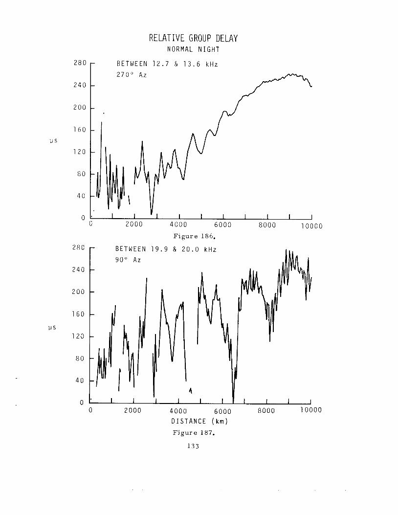
RELATIVE GROUP DELAY N O R M A L N I G H T
I
280
240
200
1 6 0
LJS
1 2 0
80
40
B E T W E E N 1 2 . 7 & 1 3 . 6 k H z
2 7 0 " A z
280
240
200
1 6 0
us 1 2 0
80
40
0
I
2000 4000 6000 8000 10000 0
F i g u r e 186.
B E T W E E N
9 0 " A 2
1
0 2 0 0 0 4000 6 0 0 0 8000 1 0 0 0 0
D I S T A N C E ( k m ) F i g u r e 187.
133
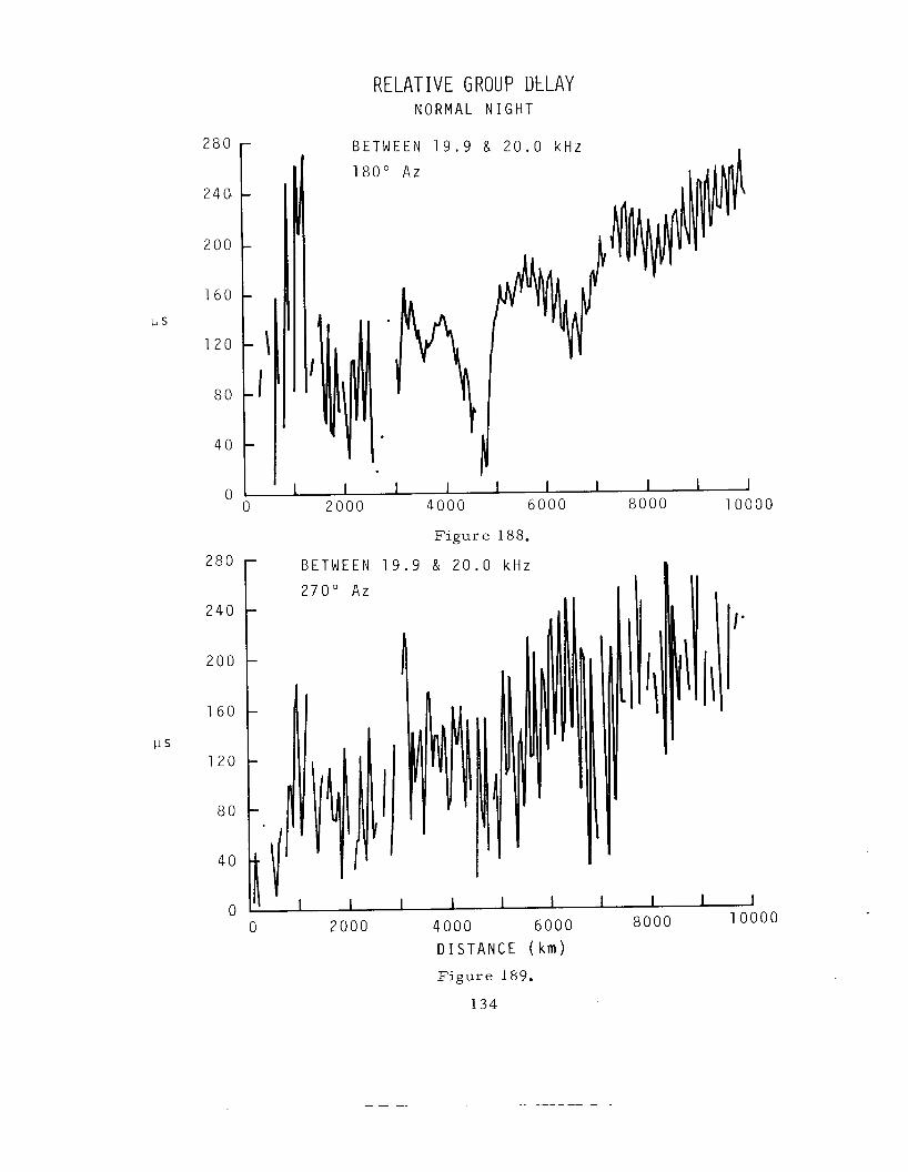
RELATIVE GROUP DELAY NORMAL NIGHT
2 8 0
2 4 0 1 200
1 6 0
1 2 0
80
4 0
0
BETWEEN 1 9 . 9 & 2 0 . 0 kHz I
A Z
4 F i g u r e 188.
BETWEEN 1 9 . 9 & 2 0 . 0 kHz
2 8 0 r 2 7 0 " Az
8 0 0 0 10000
2 4 0 -
2 0 0 -
I 1 8 0 0 0 1 0 0 0 0 0 2 0 0 0 4 0 0 0 6000
I'
DISTANCE ( k m )
Figure 189.
1 3 4
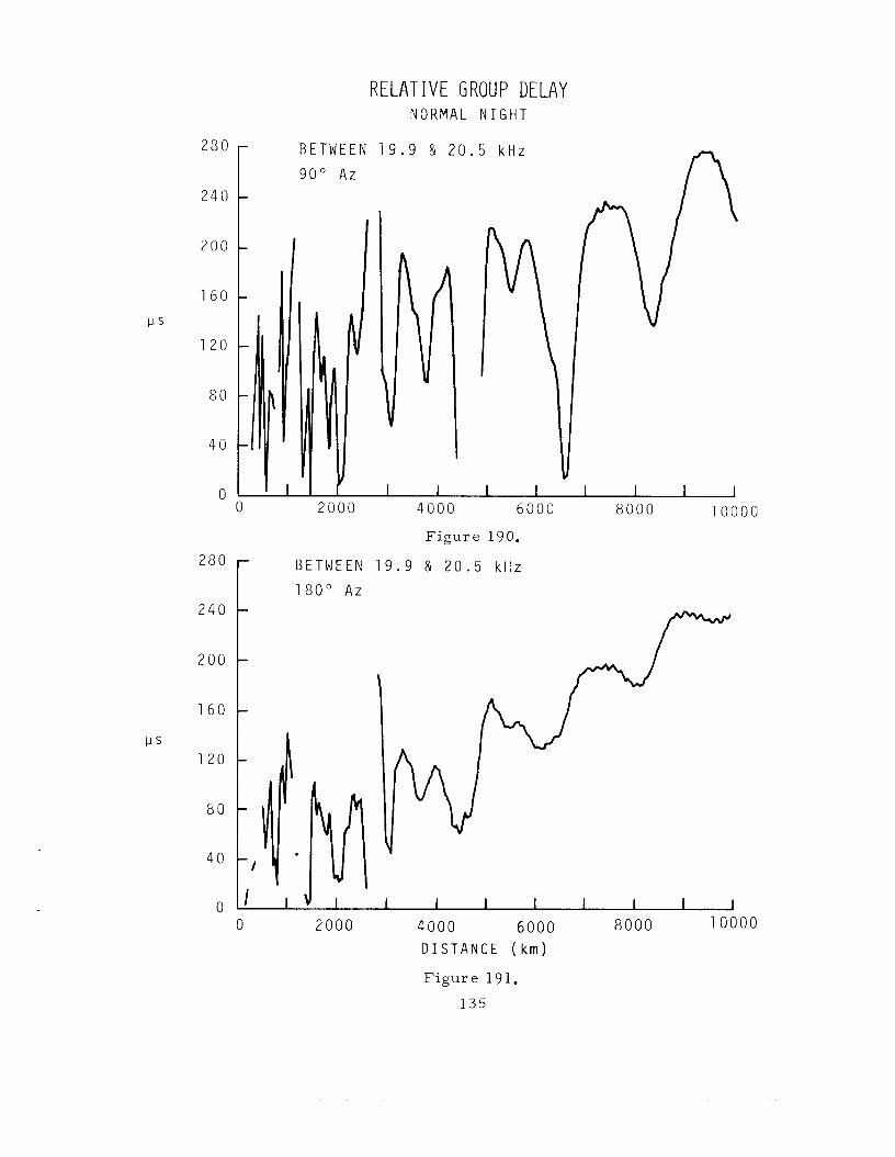
u s
RELATIVE GROUP DELAY N O R M A L N I G H T
280
240
200
1 6 0
120
80
40
0 0 2000 4000 6000 8000 10000
F i g u r e 190.
B E T W E E N 1 9 . 9 & 2 0 . 5 k H z
2 8 0 r 1 8 0 " A z 240
200
1 6 0
80
40
0 0 2000 4000 6000 8000 10000
D I S T A N C E ( k m )
F i g u r e 191.
135
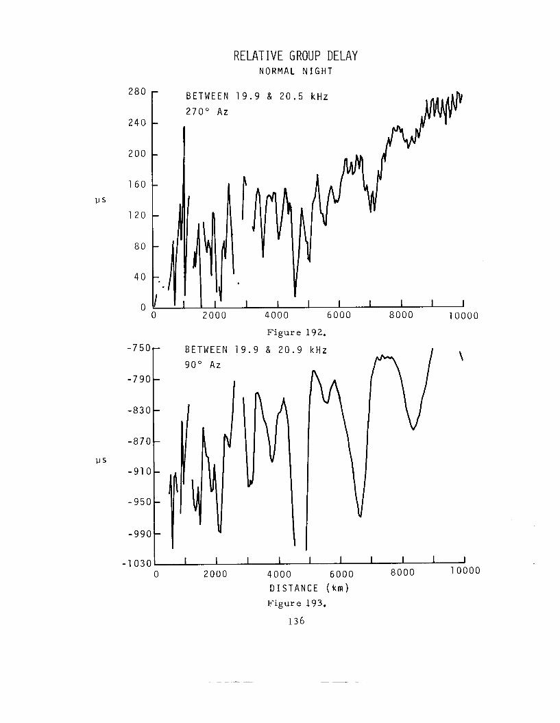
RELATIVE GROUP DELAY NORMAL N I G H T
u s
2 8 0
2 4 0
2 0 0
1 6 0
1 2 0
8 0
4 0
0
1 B E T W E E N 1 9 . 9 & 2 0 . 5 kHz r 2 7 0 " Az
t I dl""
0 2000 4 0 0 0 6 0 0 0 8 0 0 0 1 0 0 0
F i g u r e 192.
9 0 " Az I - 7 9 0 t
I
4 :I \
- 7 5 0 ~ B E T W E E N 1 9 . 9 & 2 0 . 9 kHz
0
I I I I I 1 I 1 I I 10000
- 1 0301 0 2 0 0 0 4 0 0 0 6 0 0 0 8 0 0 0
D I S T A N C E ( k m ) F i g u r e 193.
136
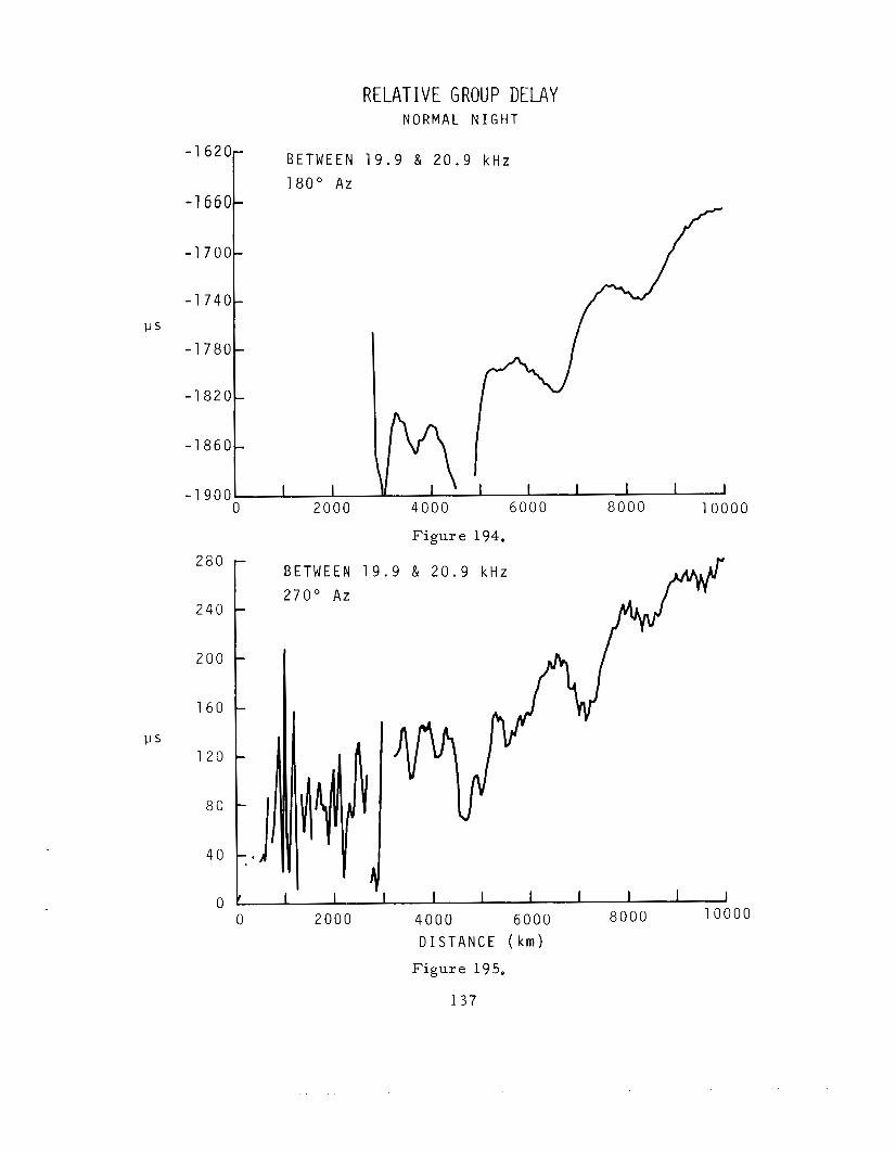
- 1 6 6 0 -
RELATIVE GROUP DELAY N O R M A L N I G H T
B E T W E E N 19.9 & 20.9 k H z
1 8 0 " Az
F i g u r e 194.
B E T W E E N 1 9 . 9 & 2 0 . 9 k H z 2 7 0 " Az
40
0 0 2 0 0 0 4000 6000 8 0 0 0 1 0 0 0 0
D I S T A N C E ( k m ) F i g u r e 195.
137
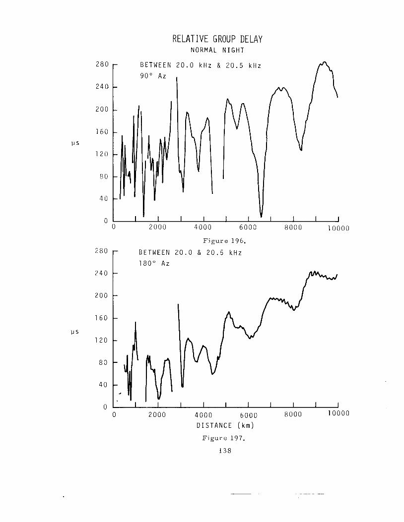
280 9 0 " Az I
2 4 a t 200
1 6 0
120
80
40
n
RELATIVE GROUP DELAY N O R M A L N I G H T
280
240
200
1 6 0
P S 120
80
40
0
- 0 2000 4000 6000 8000 1 0 0 0 0
F i g u r e 196.
BETWEEN 20.0 & 20.5 k H z
1 8 0 " Az
0 2000 4000 6000 8000 10000
DISTANCE ( k m )
F i g u r e 197,
138
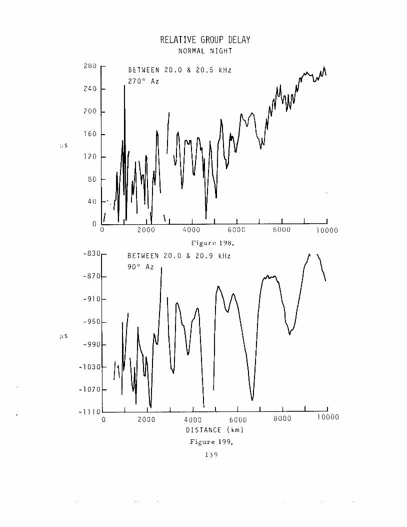
RELATIVE GROUP DELAY N O R M A L N I G H T
B E T W E E N 20.0 ti 20.5 k H z 2 7 0 " A z
280 -
2 4 0 -
200 -
cis
1 2 0
80
40 -'.
I 0 0
us
2000
B E T W E E N 90" A z
I
4000 6000 8000 10000
F i g u r e 198.
20.0 84 20.
4 - 1 1 1 0
8000 10000 0 2000 4000 6000 D I S T A N C E ( k m ) F i g u r e 199.
1 3 9
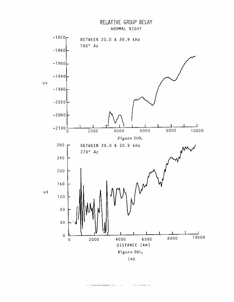
RELATIVE GROUP DELAY NORMAL N I G H T
2 4 0
2 0 0
1 6 0
BETWEEN 2 0 . 0 & 2 0 . 9 k H z 1 8 0 " Az
-
-
-
- 2 0 2 0 I-
F i g u r e 200.
BETWEEN 2 0 . 0 & 2 0 . 9 kHz
I I I I I I 1 8 0 0 0 1 0 0 0 0 4 0 0 0 6 0 0 0
D I S T A N C E ( k m )
F i g u r e 201.
140
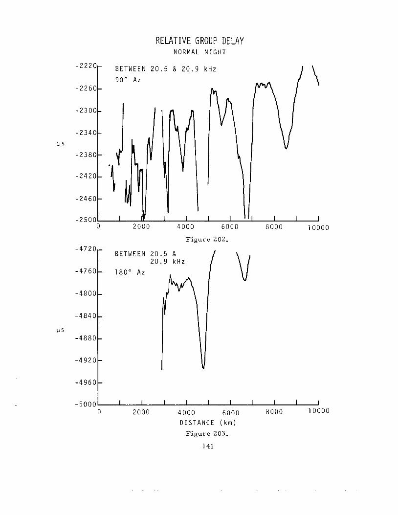
RELATIVE GROUP DELAY N O R M A L N I G H T
B E T W E E N 20.5 & 20.9 k H z 9 0 " A z
I
-24
- 24
- 2 5 0 2000 4000 6000
Figure 202.
B E T W E E N 20.5 & 20.9 k H z
8000 10000
-50001 I I 1 I 1 I 1 I I 1 0 2000 4000 6000 8000 10000
D I S T A N C E ( k m )
Figure 203.
141

280
240
200
1 6 0
1 2 0
80
40
0
RELATIVE GROUP DELAY N O R M A L N I G H T
B E T W E E N 20.5 & 2 0 . 9 k H z 2 7 0 " Az
00
Figure 204.
142
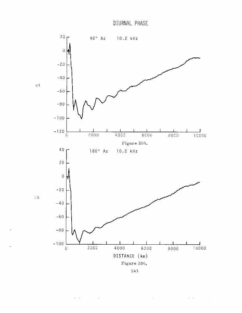
D I U R N A L PHASE
r 9 0 " A z 1 0 . 2 kHz
L!S
I - 1 2 0 I I 1 I I 1 I I I 1 0 2000 4000 6000 8000 10000
Figure 205.
40 r 1 8 0 " A z 10.2 k H z
20 c LS
0
-20
-40
- 6 0
- 8 0
- 1 00 10000 0 2000 4000 6000 8000
D I S T A N C E ( k m )
F i g u r e 206.
143

DIURNAL PHASE
2 7 0 " Az 1 0 . 2 kHz
4 0 r
4 0
2 0
0
- 2 0
P S - 4 0
- 6 0
-80
- 1 oc
F i g u r e 207.
9 0 " Az 1 2 . 2 kHz
I I I I I I 1 I I I 2000 4000 6000 a o o o 10000 0
D I S T A N C E ( k m ) F i g u r e 208.
144
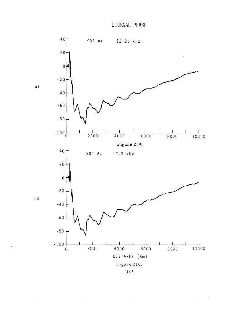
DIURNAL PHASE
40r 9 0 " Az 1 2 . 2 5 k H z
-80
- 1 o o L I I I 1 I 1 1 I I 1 2000 4000 6000 8000 10000 0
Figure 209.
9 0 " Az 1 2 . 3 k H z
I I I
- I U U I I I I I 1 I I 1 1 10000 0 2000 4000 6000 8000
D I S T A N C E ( k m )
Figure 21 0.
145
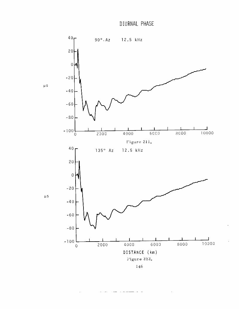
DIURNAL PHASE
9 0 " . Az 1 2 . 5 k H z
us
I I I I I I I I I I 4000 6000 8000 1 0 0 - 1 00 I
0 2000
F i g u r e 211.
1 3 5 " Az 1 2 . 5 k H z
u s
9 0 " . Az 1 2 . 5 k H z 40-
- 2 0 -
-40 -
-60 -
-80 - I I I I I I I I I I
0 2000 4000 6000 8000 1 0 0 - 1 00
F i g u r e 211.
1 3 5 " Az 1 2 . 5 k H z 40 -
20 - 1
-20 -
-40 -
-60 -
-80 -
00
I I I 1 I I I I I I 2000 4000 6000 8000 10000 - 1 00
0 D I S T A N C E ( k m )
F i g u r e 212.
146
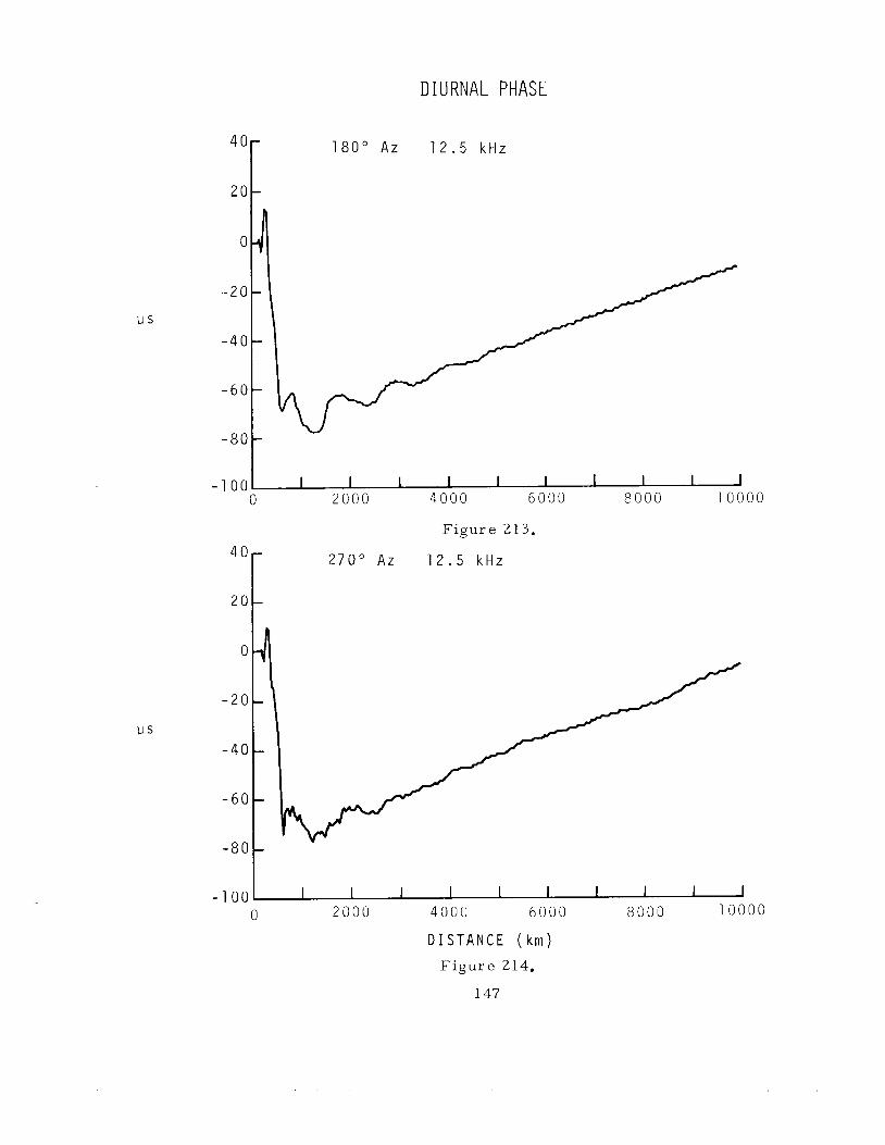
DIURNAL PHASE
2 7 0 " Az 1 2 . 5 kHz
40
20
2 o
1 8 0 " Az 1 2 . 5 kHz -
-
t
- 1 001 I 1 1 I 1 I I I I I 0 2000 4000 6000 8000 10000
2 0
2 7 0 " Az 1 2 . 5 kHz
-
- 1 0 0 1 I 1 I 1 1 I I I I I 0 2000 4000 6000 8000 10000
DISTANCE ( k m )
F i g u r e 214.
147
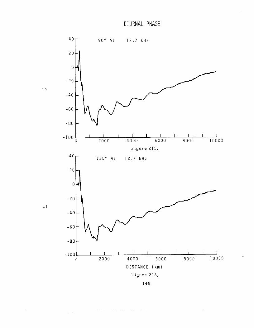
u s
40
20
0
- 2 0
-40
-60
- 8 0
- 1 0 0
DIURNAL PHASE
9 0 " Az 1 2 . 7 kHz
I I 1 I I I I I I 1 cl 2000 4000 6000 8000 10000
Figure 21 5.
40
20
0
- 2 c
- 4 c
-6C
-8C
40r - 1 3 5 " Az 1 2 . 7 kHz 1 3 5 " Az 1 2 . 7 kHz
- 1 001 I I I 1 I I 1 I I I 0 2 0 0 0 4 0 0 0 6 0 0 0 8 0 0 0 1 0 0 0 0
D I S T A N C E ( k m )
Figure 21 6.
148
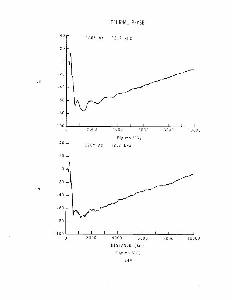
DIURNAL PHASE
4 0 r 20 I-
O
- 2 0
-60
-80
-100
4 0
2 0
0
- 2 0
u s -40
-60
-80
- 1 0 0
180" A z 1 2 . 7 kHz
F i g u r e 217.
2 7 0 " Az 1 2 . 7 k H z
I I 1 1 I 1 I I I 1 10000 0 2000 4000 6000 8000
D I S T A N C E ( k m )
F i g u r e 218.
149
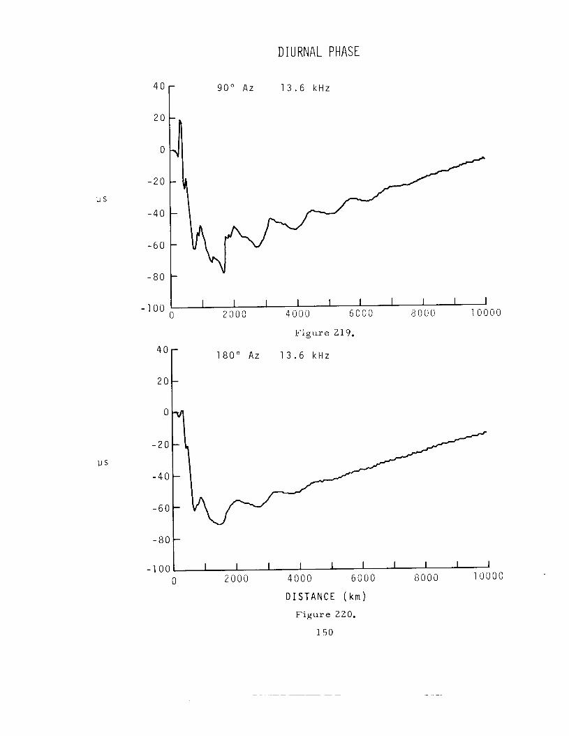
40
20
0
-20
-40
-60
-80
- 1 00
40
20
0
- 2 c
1J.S
- 4 c
-6C
-8C
- 1 01
D I U RNAL PHASE
9 0 " A z 1 3 . 6 k H z
0
F i g u r e 219. -
1 8 0 " Az 1 3 . 6 k H z
I I I 1 I I I I I I 2000 4000 6000 8000 10000 0
D I S T A N C E ( k m )
F i g u r e 220.
150
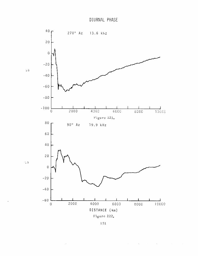
D I U R N A L PHASE
-80
- 1 0 0 .
270" A z
-
I I I I I I I I 1 1
1 3 . 6 k H z
6 0
40
0
90" Az 1 9 . 9 k H z
-
-
-20 U S
-40
-40
-60
-
151
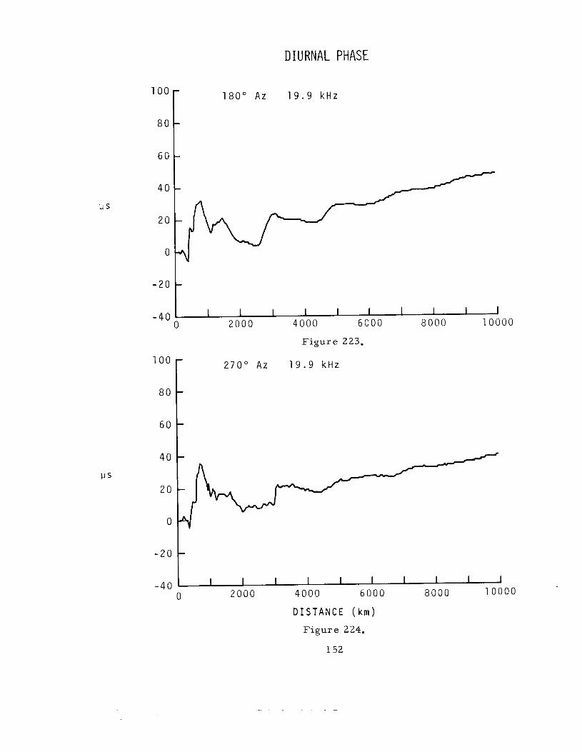
u s
1 0 0
6 0
D I URNAL PHASE
1 8 0 " Az 1 9 . 9 k H z
40
20
0
1 0 0
8 0
6 0
40 US
20
0
-20
-40
F i g u r e 2 2 3 .
2 7 0 " Az 1 9 . 9 kHz
I I I I I I I I I I 2000 4000 6000 8000 1 0 0 0 0 0
D I S T A N C E ( k m )
F i g u r e 224.
152
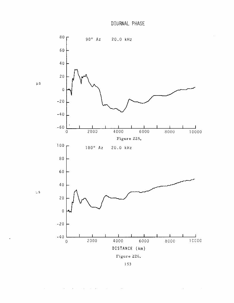
DIURNAL PHASE
r 9 0 " Az 2 0 . 0 kHz
-
-
-
- I
I 1 I I I I I I I 1
80
60
40
20
0
-20
-40
- 6 0
100
8 0
6 0
40
20
0
-20
-40 0
- 1 8 0 " Az 2 0 . 0 kHz
I 2000
I I I I I 4000 6000 8000
D I S T A N C E ( k m ) F i g u r e 226.
153
I 10000
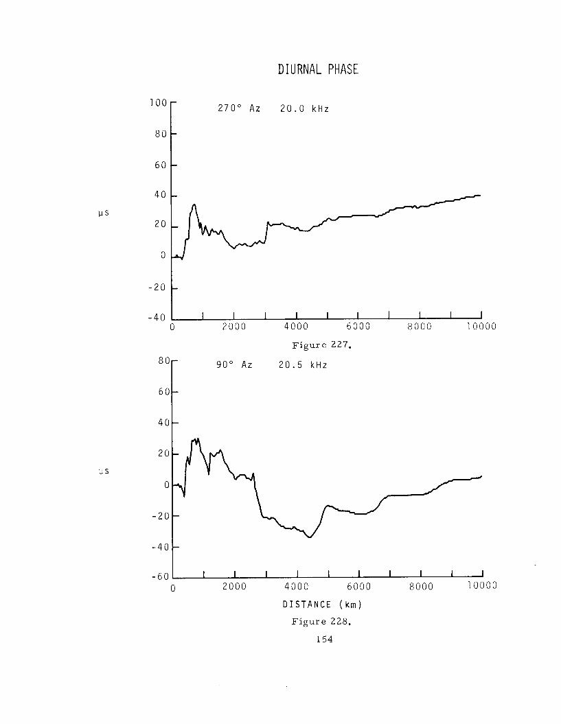
DIURNAL PHASE
1 0 0 -
8 0
60
40
2 7 0 " Az 2 0 . 0 kHz
-
-
-
-40 I I I I I I I 1 I 1 I 0 2000 4000 6000 8000 10000
c 90" Az 2 0 . 5 kHz
-
-
us
-
I 1 I 1 I I I 1 I 1
8 0
60
40
2 0
0
- 2 0
-40
-60
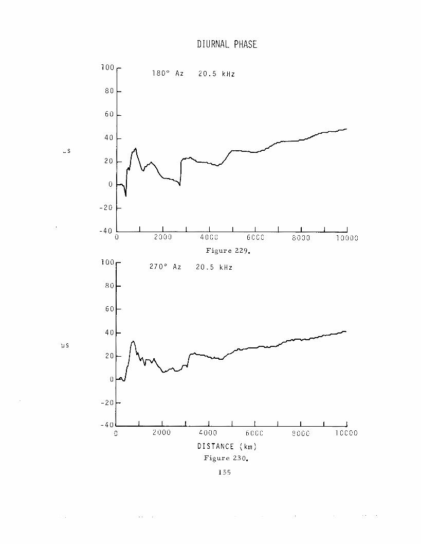
D I U R N A L PHASE
- 2 0
1 8 0 " Az 2 0 . 5 kHz
60
- - 2 0 -
00
10000 0 2000 4000 6000 8000 D I S T A N C E ( k m )
F i g u r e 230.
155
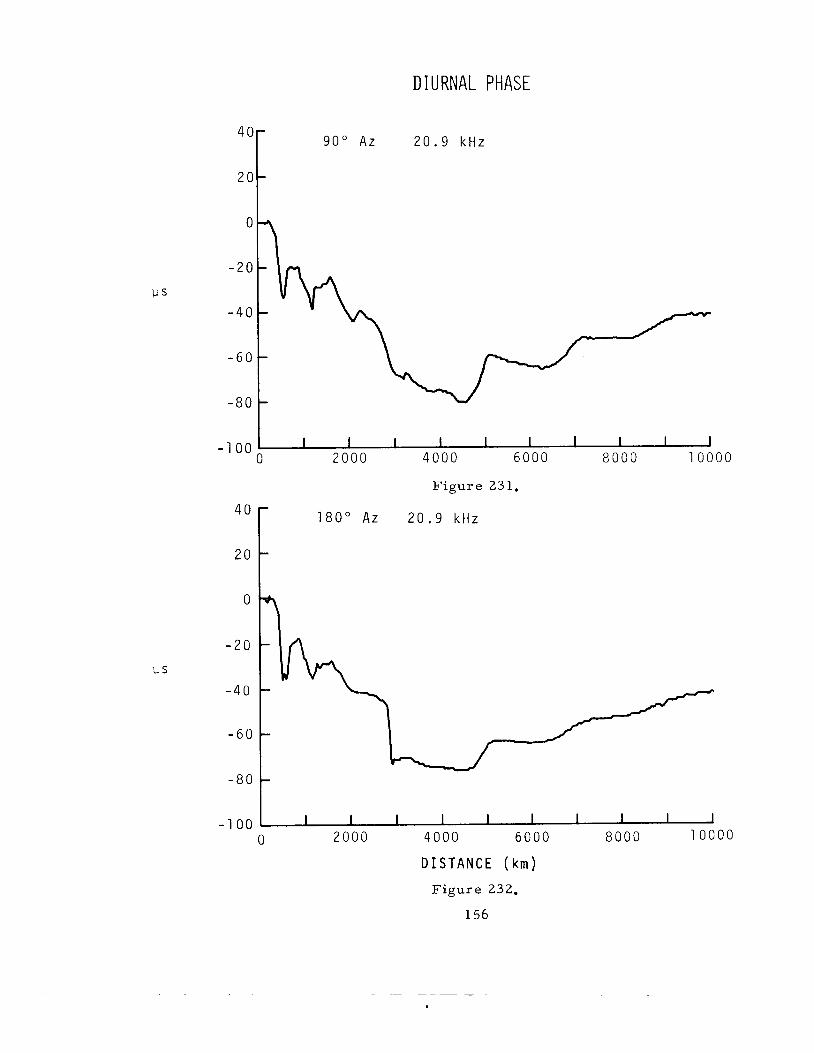
D I U RNAL PHASE
u s
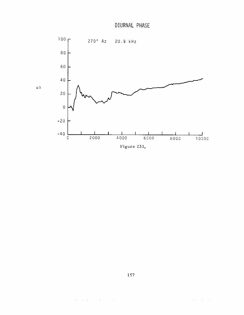
1 0 0
80
60
40 U S
20
0
-20
-40
DIURNAL PHASE
2 7 0 " P,z 20.9 k H z
I 1 I I 1 I I I I 1
1 5 7
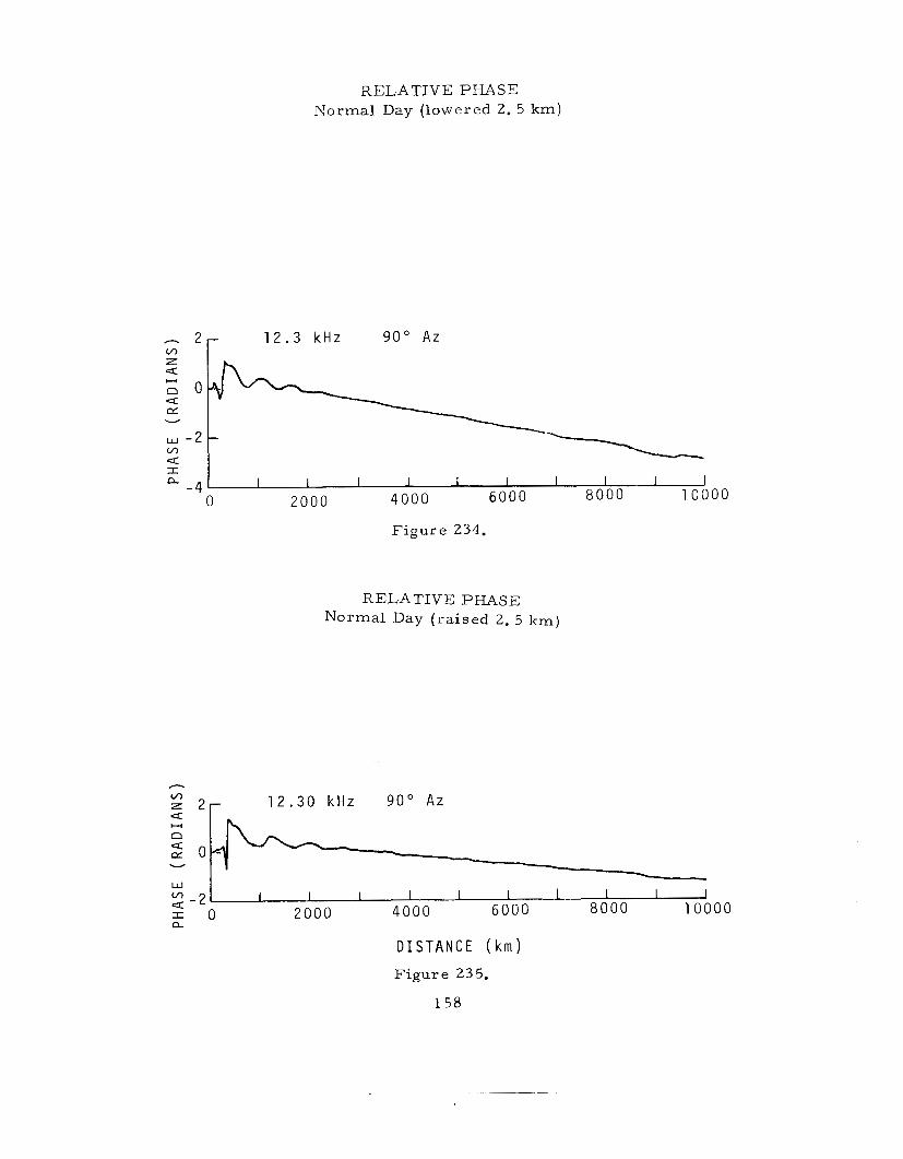
- 2
Q
0 Q @L
H
v
w v,
U n o Q @L v
0 4 - I I 1 I I I I I d
w - 2 v, Q I
RELATIVE PHASE N o r m a l Day ( lowered 2. 5 k m )
- 1 2 . 3 k H z 9 0 " A z
a 1 I I 1 I I 1 I I I 0 2000 4000 6 0 0 0 8000 10000 - 4 I
Figure 234.
RELATIVE PHASE N o r m a l Day ( r a i s e d 2. 5 k m )
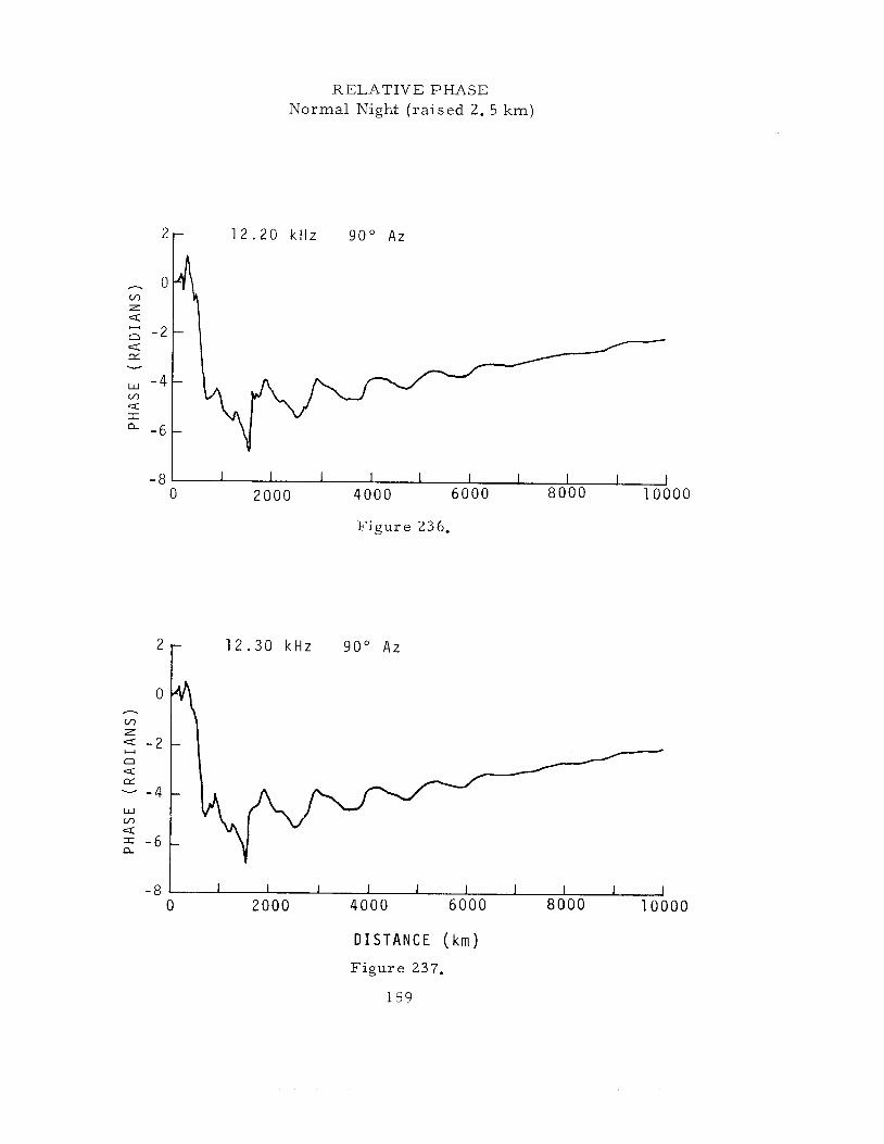
RELATIVE PHASE N o r m a l Night (raised 2. 5 k m )
2
0 h
v, z Q - 2 n
- - 4
H
Q e
W VI < I -6 n
- 8
- 1 2 . 2 0 k H z 9 0 " Az
I 1 1 I 1 I I I I I 0 2 0 0 0 4 0 0 0 6 0 0 0 8 0 0 0 1 0 0 0 0
F i g u r e 236,
- 1 2 . 3 0 k H z 9 0 " A z
1 1 1 I 1 I I I I I 0 2 0 0 0 4 0 0 0 6000 8000 10000
D I S T A N C E ( k m )
F i g u r e 237.
159
RELATIVE PHASE N o r m a l Day (sea w a t e r )
1 0 . 2 kHz 'r 9 0 " Az
- 0 m z Q
Q
H
n - 2 -
w - 4 - m 5 I a
- 6 -
I 1 1 1 I I I 1 1 I -8 6000 8000 10000 -
0 2000 4 0 0 0 F i g u r e 238.
I 1 1 1 I I I 1 1 I -8 6000 8000 10000
r i g u r e 238.
RELATIVE PHASE N o r m a l Day ( lowered 2. 5 km)
- 2 m
e W
w - 2 m Q I a -4
1 2 . 2 kHz 9 0 " Az r
I I I I 1 1- 4000 6000 8000 100 0 2000 F i g u r e 239.
00
RELATIVE PHASE N o r m a l Day ( r a i s e d 2. 5 km)
1 2 . 2 0 kHz 9 0 " Az m z 2 - 4
n
e o
m 1 I I--- 5 - 2
H
4
W
w - -
I O 2000 4000 6000 8000 10000 a
DISTANCE ( k m )
F i g u r e 240.
160
RELATIVE PHASE Normal Day ( s e a w a t e r )
1 2 . 5 kt iz 9 0 " A 2
-4
0 n
m z Q
- 2 n < CY v
-4 w m Q I a - 6
1 I I 1 1 I I I I I 0 2000 4000 6000 8000 100
F i g u r e 241. RELATIVE PHASE
Bain and May P r o f i l e
-
-
00
- 8 8 u - i d 0 2000 4000 6000 8000 10000
F i g u r e 242.
1 0 . 2 k H z 9 0 " A z RELATIVE PHASE
D I S T A N C E ( k n i )
F i g u r e 243.
161
RELATIVE PHASE N o r m a l Day ( s e a w a t e r )
- 2 - z
1 2 . 7 kHz 9 0 " Az
I I 1 I I 1 I 1 I 1 6000 8000 10000 -4 I
0 2000 4 0 0 0
F i g u r e 244.
h
v, z 4
0 Q e
U
V
w m 4 I a
1 2 . 5 kHz 9 0 " Az RELATIVE PHASE
0
- 2
- 4 L L J 0 2000 4000 6000 8000 10000
m
Q z 2
e o
4 - 2
U
n 4
V
w m
F i g u r e 245.
- RELATIVE PHASE 1 2 . 5 kHz 9 0 " Az Deeks 1200 P r o f i l e
2-
I I 1 I 1 I I I 1 I 2000 4000 6000 8000 10000 I O a
D I S T A N C E ( k m )
F i g u r e 246.
1 6 2
R EL A TI V E P EM S E Normal Day (sea wate r )
20.0 KHz 90" A 2 'r * 3 z 4
w
5 * -4
- 2 w
1 2 . 7 k H z 90" A z RELATIVE; PHASE
F i g u r e 248.
- 1 2 . 7 k H z 90" P,z R E L A T I V E PHASE Decks i z o o P ro f i i e *- ------ - .-
D I S T A N C E ( A r r i )
F i g u r e 249.
163

RELATIVE PHASE Bain and May Profile
20.0 kHz 90" Az
F i g u r e 250.
RELATIVE PHASE Deeks 1200 P r o f i l e
20.0 k H z 9 0 " A z l o r
0 2000 4000 6 0 0 0 8 0 0 0 1 0 0 0 0
D I S T A N C E ( k m )
F i g u r e 251.
164
RELATIVE C R O U P DEX,A.( N o r m a l Day (sea w a t e r )
280
240
200
1 6 0
i i s 120
80
40
0
280
240
200
1 6 0
lis 1 2 0
80
40
0
1 2 . 5 t o 1 2 . 7 k H z
2000 4000 6000 8000 10000 F i g u r e 252,
RELATIVE GROUP DELAY Deeks 1200 Profile
1 2 . 5 t o 1 2 . 7 k H z
9 0 " A z -
-
-
-
2000 4000 6000 8000 10000 D I S T A N C E ( k i n )
F i g u r e 253.
165
280
240
200
1 6 0
U S
1 2 0
80
40
0
R E L A T I V E GROUP DELAY Bain and May Profile
1 1 1 1 I 1 I 1 1 I 2000 4000 6000 a o o o 1 0 0 0 0
F i g u r e 254.
166
NBS TECHNICAL
PERIODICALS
JOURNAL OF RESEARCH reports National Bureau of Standards research and development in physics, mathematics, chemistry, and engineering. Comprehensive scientific papers give complete details of the work. including laboratory data, experimental procedures, and theoretical and mathematical analy- ses. Illustrated with photographs, drawings, and charts.
Published in three sectionc, available separately:
Physics and Chemistry
Papers of interest primarily to scientists working in these .fields. This section covers a broad range of physical and chemical research, with major emphasis on standards of physical measurement, fundamental constants, and properties of matter. Issued six times a year. Annual subscription: Domestic, $9.50; $2.25 additional for foreign mailing.
0 Mathematical Sciences
Studies and compilations designed mainly for the mathematician and theoretical physicist. Topics in mathematical statistics, theory of experiment design, numerical analysis, theoretical physics and chemis- ty, logical design and programming of computers and computer systems. Short numerical tables. Issued quarterly. Annual subscription : Domestic, $5.00; $1.25 additional for foreign mailing.
Engineering and Instrumentation
Reporting results of interest chiefly to the engineer and the applied scientist. This section includes many of the new developments in instrumentation resulting from the Bureau's work in physical measurement, data processing, and development of test methods. I t will also cover some of the work in acoustics, applied mechanics, building research, and cryogenic engineering. Issued quarterly. Annual subscription : Domestic, $5.00; $1.25 additional for foreign mailing.
TECHNICAL NEWS BULLETIN
The best single source of information concerning the Bureau's research. developmental, cooperative, and publication activities, this monthly publication is desiqned for the industry-oriented individual whose daily work involves intimate contact with science and technology-for engineers, chemists, physicists, re- search managcrs, product-development managers, and company executtvec. Annual subscription : Domestic, $3.00; $1 .OO additional for foreign mailing.
PUBLICATIONS
NONPERIODICALS
Applied Mathematics Series. Mathematical tables, manuals, and studies.
Building Science Series. Research results, test methods, and performance criteria of building ma- terials, components, systems, and structures.
Handbooks. Recommended codes of engineering and industrial practice (including safety codes) de- veloped in cooperation with interested industries, professional organizations, and regulatory bodies.
Special Publications. Proceedings of NBS confer- ences, bibliographies, annual reports, wall charts, pamphlets, etc.
Monographs. Major contributions to the technical literature on various subjects related to the Bureau's scientific and technical activities.
National Standard Reference Data Series. NSRDS provides quantitative data on the physical and chemical properties of materials, compiled from the world's literature and critically evaluated.
Product Standards. Provide requirements for sizes, types, quality, and methods for testing various indus- trial products. These standards are developed co- operatively with interested Government and industry groups and provide the basis for common understand- ing of product characteristics for both buyers and sellers. Their use is voluntary.
Technical Notes. This series consists of communi- cations and reports (covering both other agency and NBS-sponsored work) of limited or transitory interest.
Federal Information Processing Standards Publications. This series is the official publication within the Federal Government for information on standards adopted and promulgated under the Public Law 89-306, and Bureau of the Budget Circular A-86 entitled, Standardization of Data Elements and Codes in Data Systems.
Consumer Information Series. Practical informa- tion, based on NBS research and experience, covering areas of interest to the consumer. Easily understand- able language and illustrations provide useful back- ground knowledge for shopping in today's technolog- ical marketplace.
NRS Special Publication 305, Supplement 1, Publications of the NBS, 1968-1969. When order- ing, include Catalog No. C 13.10: 305. Price $4.50 ; $1.25 additional for foreign mailing.
Order NBS publications from: Superintendent of Documents Government Printing Office Washington, D.C. 20402