NBER WORKING PAPER SERIES

REDUCING FORECLOSURES:NO EASY ANSWERS

Christopher FooteKristopher Gerardi

Lorenz GoettePaul Willen

Working Paper 15063http://www.nber.org/papers/w15063

NATIONAL BUREAU OF ECONOMIC RESEARCH1050 Massachusetts Avenue

Cambridge, MA 02138June 2009

The views in this paper are our own and not necessarily those of the Federal Reserve Banks of Bostonor Atlanta. the Federal Reserve System, or the National Bureau of Economic Research. Andreas Fusterprovided both first-rate research assistance and excellent comments and suggestions. We would liketo thank, without implicating, Daron Acemoglu, Larry Cordell, Jeff Fuhrer, Eileen Mauskopf, ChristopherMayer, Atif Mian, James Nason, Julio Rotemberg, and Hui Shan for helpful comments and suggestions.We are also grateful for the help that Mark Watson and Kevin Shruhan provided us in working withthe LPS data. Any remaining errors are our own.

NBER working papers are circulated for discussion and comment purposes. They have not been peer-reviewed or been subject to the review by the NBER Board of Directors that accompanies officialNBER publications.

© 2009 by Christopher Foote, Kristopher Gerardi, Lorenz Goette, and Paul Willen. All rights reserved.Short sections of text, not to exceed two paragraphs, may be quoted without explicit permission providedthat full credit, including © notice, is given to the source.

Reducing Foreclosures: No Easy AnswersChristopher Foote, Kristopher Gerardi, Lorenz Goette, and Paul WillenNBER Working Paper No. 15063June 2009JEL No. R2

ABSTRACT

This paper takes a skeptical look at a leading argument about what is causing the foreclosure crisisand distills some potential lessons for policy. We use an economic model to focus on two key decisions:the borrower’s choice to default on a mortgage and the lender’s subsequent choice whether to renegotiateor “modify” the loan. The theoretical model and econometric analysis illustrate that “unaffordable”loans, defined as those with high mortgage payments relative to income at origination, are unlikelyto be the main reason that borrowers decide to default. In addition, this paper provides theoretical resultsand empirical evidence supporting the hypothesis that the efficiency of foreclosure for investors isa more plausible explanation for the low number of modifications to date than contract frictions relatedto securitization agreements between servicers and investors. While investors might be foreclosingwhen it would be socially efficient to modify, there is little evidence to suggest they are acting againsttheir own interests when they do so. An important implication of our analysis is that the extensionof temporary help to borrowers suffering adverse life events like job loss could prevent more foreclosuresthan a policy that makes mortgages more “affordable” on a long-term basis.

Christopher FooteFederal Reserve Bank of BostonResearch Department, T-8PO Box 55882Boston, MA 02205Chris.Foote@bos.frb.org

Kristopher GerardiFederal Reserve Bank of Atlanta1000 Peachtree St. NEAtlanta, GA 30309kristopher.gerardi@atl.frb.org

Lorenz GoetteUniversity of GenevaDepartment of Economics40 Bd du Pont d’ArveGeneva 1211, Switzerlandlorenz.goette@unige.ch

Paul WillenResearch DepartmentFederal Reserve Bank of BostonP.O. Box 55882Boston, MA 02210and NBERwillen968@yahoo.com

1 Introduction

One of the most important challenges now facing U.S. policymakers stems from the tide

of foreclosures that now engulfs the country. There is no shortage of suggestions for how

to attack the problem. One of the most influential strands of thought contends that the

crisis can be attenuated by changing the terms of “unaffordable” mortgages. It is thought

that modifying mortgages is not just good for borrowers in danger of losing their homes but

also beneficial for lenders, who will recover more from modifications than they would from

foreclosures. Proponents of this view, however, worry that without government intervention,

this win-win outcome will not occur. Their concern is that the securitization of mortgages

has given rise to contract frictions that prevent lenders and their agents (loan servicers)

from carrying out modifications that would benefit both borrowers and lenders.

In this paper, we take a skeptical look at this argument. Using both a theoretical

model and some loan-level data, we investigate two economic decisions, the borrower’s

decision to default on a mortgage and the lender’s choice between offering a loan modification

and foreclosing on a delinquent loan. We first study the “affordability” of a mortgage,

typically measured by the DTI ratio, which is the size of the monthly payment relative to the

borrower’s gross income.1 We find that the DTI ratio at the time of origination is not a strong

predictor of future mortgage default. A simple theoretical model explains this result. While

a higher monthly payment makes default more likely, other factors, such as the level of house

prices, expectations of future house price growth and intertemporal variation in household

income, matter as well. Movements in all of these factors have increased the probability of

default in recent years, so a large increase in foreclosures is not surprising. Ultimately, the

importance of affordability at origination is an empirical question and the data show scant

evidence of its importance. We estimate that a 10-percentage-point increase in the DTI

ratio increases the probability of a 90-day-delinquency by 7 to 11 percent, depending on

the borrower.2 By contrast, an 1-percentage-point increase in the unemployment rate raises

this probability by 10-20 percent, while a 10-percentage-point fall in house prices raises it

by more than half.

1DTI ratio stands for “debt-to-income” ratio. A more appropriate name for this ratio is probably“payment-to-income” ratio, but we use the more familiar terminology. Throughout this paper, we defineDTI as the ratio of mortgage-related payments to income, rather than all debt payments; this is sometimescalled the “front end” DTI.

2As explained below, these estimates emerge from a duration model of delinquency that are based oninstantaneous hazard rates. So, the statement that an 10-percentage-point increase in DTI increases theprobability of 90-day delinquency by 7 percent means that the DTI increase multiplies the instantaneousdelinquency hazard by 1.07, not that the DTI increase raises the probability of delinquency by 7 percentagepoints.

1

The fact that origination DTI explains so few foreclosures should not surprise economists,

given the mountain of economic research on the sources and magnitude of income variation

among U.S. residents. The substantial degree of churning in the labor market, combined

with the trial-and-error path that workers typically follow to find good job matches, suggests

that income today is an imperfect predictor of income tomorrow. Consequently, a mortgage

that is affordable at origination may be substantially less so later on, and vice versa.

We then address the question of why mortgage servicers, who manage loans on behalf

of investors in mortgage-backed securities, have been unwilling to make mass loan modifi-

cations. The evidence that a foreclosure loses money for the lender seems compelling. The

servicer typically resells a foreclosed house for much less than the outstanding balance on the

mortgage, in part because borrowers who lose their homes have little incentive to maintain

them during the foreclosure process.3 This would seem to imply that the ultimate owners

of a securitized mortgage, the investors, lose money when a foreclosure occurs. Estimates of

the total gains to investors from modifying rather than foreclosing can run to $180 billion,

more than 1 percent of GDP. It is natural to wonder why investors are leaving so many

$500 bills on the sidewalk. While contract frictions are one possible explanation, another is

that the gains from loan modifications are in reality much smaller or even nonexistent from

the investor’s point of view.

We provide evidence in favor of the latter explanation. First, the typical calculation

purporting to show that an investor loses money when a foreclosure occurs does not capture

all relevant aspects of the problem. Investors also lose money when they modify mortgages

for borrowers who would have repaid anyway, especially if modifications are done en masse,

as proponents insist they should be. Moreover, the calculation ignores the possibility that

borrowers with modified loans will default again later, usually for the same reason they

defaulted in the first place. These two problems are empirically meaningful and can easily

explain why servicers eschew modification in favor of foreclosure.

Turning to the data, we find that the evidence of contract frictions is weak, at least if

these frictions result from the securitization of the loan. Securitization agreements generally

instruct the servicer to behave “as if” it owned the loan in its own portfolio, and the data

are consistent with that principle. Using a dataset that includes both securitized and non-

securitized loans, we show that these two types of loans are modified at about the same

rate. While there is room for further empirical work on this issue, these results minimize

the likely importance of contract-related frictions in the modification decision. Even though

3An even more important reason that lenders rarely recover the full balance of the mortgage is that theborrower owed more on the home than the home was worth. Below, we show that negative equity is anecessary condition for foreclosure; people rarely lose their homes when they enjoy positive equity.

2

it may be in society’s interest to make modifications (because of the large externalities from

foreclosure), it may not be in the lender’s interest to do so, whether or not this lender is an

investor in a mortgage-backed security or a portfolio lender.4

Our skepticism about the arguments discussed above is not meant to suggest that gov-

ernment has no role in reducing foreclosures. Nor are we arguing that the crisis is completely

unrelated to looser lending standards, which saddled borrowers with high-DTI mortgages,

or interest rates that reset to higher levels a few years into the loans.5 Rather, we argue that

a foreclosure-prevention policy that is focused on high-DTI ratios and interest-rate resets

may not address the most important source of defaults. In the data, this source appears to

be the interaction of falling prices and adverse life events, such as job loss.

The remainder of this paper is organized as follows. Section 2 outlines a simple model

of the default decision that helps organize ideas about potential sources of the foreclosure

crisis. Section 3 shows that, as would be implied by the simple model, the affordability of a

mortgage at origination as measured by DTI is not a strong predictor of mortgage default,

especially compared with other variables that reflect income volatility and falling house

prices in a fundamental way. Section 4 adapts the model to encompass the decision of the

lender to offer a modification, and then provides evidence that securitization contracts are

not unduly preventing modifications. Section 5 concludes with some lessons for foreclosure-

reduction policy that are suggested by our results.

2 Affordability and Foreclosure: Theory

One of the most commonly cited causes of the current foreclosure crisis is the mass

origination of unaffordable or unsustainable mortgages. Ellen Harnick, the senior policy

counsel for the Center for Responsible Lending, characterized the crisis this way when she

recently testified before Congress:

The flood of foreclosures we see today goes beyond the typical foreclosures of

years past, which were precipitated by catastrophic and unforeseen events such as

job loss, divorce, illness, or death. The current crisis originated in losses triggered

by the unsustainability of the mortgage itself, even without any changes in the

families’ situation, and even where the family qualified for, but was not offered,

4A foreclosure imposes externalities on society when, for example, a deteriorating foreclosed home drivesdown house prices for the entire surrounding neighborhood.

5For a discussion of the role of looser lending standards, see Mian and Sufi (2009) and Dell’Ariccia, Igan,and Laeven (2009).

3

a loan that would have been sustainable.6

The claim that the foreclosure crisis results from unaffordable or unsustainable loans has

been endorsed by a number of influential policy analysts.7 But the concept of “unaffordabil-

ity” is rarely defined precisely. To economists, something is unaffordable if it is unattainable

under any circumstances, even temporarily. For example, an economist might say: “For me,

the penthouse apartment at the Time Warner Center in New York is unaffordable ($50

million when finished in 2004).” But a non-economist might say, “For me, the dry-aged

ribeye at Whole Foods ($19.99 a pound) is unaffordable.” The problem is that, for most

Americans, a regular diet of ribeye steaks is attainable; a consumption bundle that includes

two pounds of ribeye every night is not impossible for most families. They do not choose this

bundle because of relative prices: the tradeoff between the ribeye and other consumption

is unappealing (for example, the family might prefer a new car). In this case, economists,

if they were being precise, would say that the ribeye was “affordable” but “too expensive.”

Along the same lines, economists might argue that an unaffordable mortgage is one that

is really too expensive, in the sense that the benefits that come with making payments on

the mortgage no longer outweigh the opportunity costs of doing so. In the next subsection,

we build a simple model of these benefits and costs in order to evaluate what makes a bor-

rower decide that a mortgage is unaffordable and thus to default on it. In describing this

model, we will use the common usage definition of “affordable,” though we really mean “too

expensive.”

2.1 A simple model

Assume a two-period world (t = 1, 2), with two possible future states, good and bad.

The good state occurs with probability αG, while the bad state occurs with probability αB

(where αB = 1 − αG). In the first period, the value of the home is P1 with a nominal

mortgage balance of M1. In this period, the borrower decides between making the mortgage

payment, a fraction m of the mortgage balance M1, and staying in the home, or stopping

payment and defaulting. Because this is a two-period model, we assume that in the second

6Harnick (2009), p. 5.7A recent report from the Congressional Oversight Panel of the Troubled Asset Recovery Program (here-

after denoted COP) states that “[t]he underlying problem in the foreclosure crisis is that many Americanshave unaffordable mortgages” (COP report, p. 16). The report adds that the unaffordability problem arisesfrom five major factors: (1) the fact that many mortgages were designed to be refinanced and cannot berepaid on their original terms, (2) the extension of credit to less creditworthy borrowers for whom home-ownership was inappropriate, (3) fraud on the part of brokers, lenders, and borrowers, (4) the steering ofborrowers who could qualify for lower cost mortgages into higher priced (typically subprime) mortgages,and (5) the recent economic recession.

4

period the borrower either sells the home or defaults on the mortgage. If the good state

occurs, the price of the house in the second period is P G2 , while if the bad state occurs, the

price is P B2 . We will assume that P B

2 < M2, where M2 is the remaining nominal mortgage

balance in the second period.

The first key insight of the model is that if equity is positive, the borrower will never

default on the house. Selling dominates foreclosure when equity is positive because the

borrower has to move out either way and the former strategy yields cash while the latter

does not. Exactly what constitutes positive equity is a bit tricky empirically. Borrowers

have to pay closing costs to sell the house and may be forced to accept a lower price if they

sell in a hurry. Thus, the balance of the mortgage may be slightly less than the nominal

value of the home, but with these extra expenses factored into the equation, the borrower

may not have positive equity to extract.

The empirical evidence on the role of negative equity in causing foreclosures is over-

whelming and incontrovertible. Household-level studies show that the foreclosure hazard

for homeowners with positive equity is extremely small but rises rapidly as equity approaches

and falls below zero. This estimated relationship holds both over time and across localities,

as well as within localities and time-periods, suggesting that it cannot result from the effect

of foreclosures on local-level house prices.8

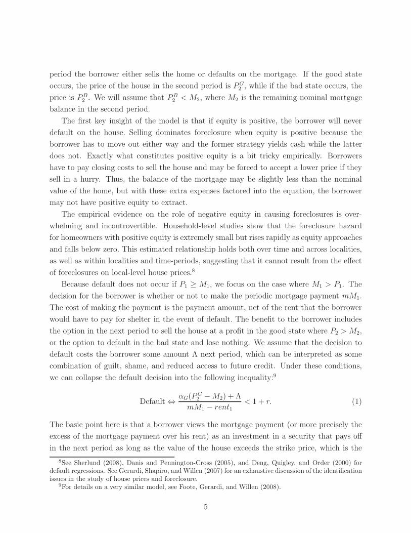
Because default does not occur if P1 ≥ M1, we focus on the case where M1 > P1. The

decision for the borrower is whether or not to make the periodic mortgage payment mM1.

The cost of making the payment is the payment amount, net of the rent that the borrower

would have to pay for shelter in the event of default. The benefit to the borrower includes

the option in the next period to sell the house at a profit in the good state where P2 > M2,

or the option to default in the bad state and lose nothing. We assume that the decision to

default costs the borrower some amount Λ next period, which can be interpreted as some

combination of guilt, shame, and reduced access to future credit. Under these conditions,

we can collapse the default decision into the following inequality:9

Default ⇔αG(P G

2 − M2) + Λ

mM1 − rent1< 1 + r. (1)

The basic point here is that a borrower views the mortgage payment (or more precisely the

excess of the mortgage payment over his rent) as an investment in a security that pays off

in the next period as long as the value of the house exceeds the strike price, which is the

8See Sherlund (2008), Danis and Pennington-Cross (2005), and Deng, Quigley, and Order (2000) fordefault regressions. See Gerardi, Shapiro, and Willen (2007) for an exhaustive discussion of the identificationissues in the study of house prices and foreclosure.

9For details on a very similar model, see Foote, Gerardi, and Willen (2008).

5

outstanding balance on the mortgage. If the return on the investment exceeds the alternative

investment, here assumed to be the riskless rate, then the borrower stays in the home. If

instead the return falls short, then the borrower decides that the riskless asset is a better

investment and defaults.

Thus far, income appears to play no role in the default decision. In this sense, our

model follows the traditional option-theoretic analyses of the mortgage default decision, in

which the mortgage is viewed as a security priced by arbitrage, and household income is

irrelevant.10

The problem with the model described above is that it gives no role to individual hetero-

geneity, except potentially through differences in Λ. According to the model, all borrowers

living in similar houses with similar mortgages should default at roughly the same time.

Yet, in the data, we observe enormous heterogeneity in default behavior across otherwise

similar households. Moreover, there is a pattern to this heterogeneity: households that

suffer income disruptions default much more often than households that do not; younger

homeowners default more often; and households with few financial resources default more

often.

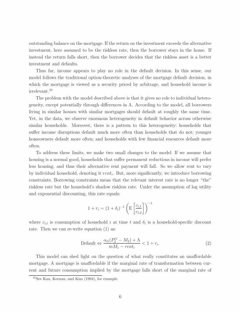
To address these limits, we make two small changes to the model. If we assume that

housing is a normal good, households that suffer permanent reductions in income will prefer

less housing, and thus their alternative rent payment will fall. So we allow rent to vary

by individual household, denoting it renti. But, more significantly, we introduce borrowing

constraints. Borrowing constraints mean that the relevant interest rate is no longer “the”

riskless rate but the household’s shadow riskless rate. Under the assumption of log utility

and exponential discounting, this rate equals:

1 + ri = (1 + δi)−1

(

E

[ci,1

ci,2

])−1

where ci,t is consumption of household i at time t and δi is a household-specific discount

rate. Then we can re-write equation (1) as:

Default ⇔αG(P G

2 − M2) + Λ

mM1 − renti< 1 + ri. (2)

This model can shed light on the question of what really constitutes an unaffordable

mortgage. A mortgage is unaffordable if the marginal rate of transformation between cur-

rent and future consumption implied by the mortgage falls short of the marginal rate of

10See Kau, Keenan, and Kim (1994), for example.

6

substitution. What makes a mortgage “unaffordable,” that is, too expensive?

1. Low house price appreciation. A higher probability of price appreciation (higher

αG) increases the expected return to staying in the house. In this sense, our treatment

is similar to the standard user cost calculation in the literature, whereby increased

house price appreciation lowers the cost of owning a home.11

2. High monthly payments. All else equal, higher m makes the mortgage less at-

tractive. This is consistent with the views expressed in the quote that opened in

this section: Many families, for one reason or another, took on mortgages with high

payments that are likely to dissuade them from keeping their mortgage current. Typ-

ically, the burden of a mortgage’s payments at origination is measured by the DTI

ratio. Thus, analysts who believe that this type of unaffordability is at the heart of

the crisis often support proposals designed to lower DTI ratios on a long-term basis.

3. Permanent and transitory shocks to income. Permanent shocks lower renti.

Also, if the borrower is constrained, then a transitory shock that leads to a lower

level of income will lead to high consumption growth and thus a high shadow riskless

rate, which makes staying less attractive. The quote that opens this chapter expresses

the view that income shocks were important drivers of foreclosure in the past, but

that these shocks are less important today. However, if income shocks are in fact the

most important source of distress in the housing market, then a policy that grants

troubled borrowers substantial but temporary assistance could be effective. Tempo-

rary assistance may not help borrowers facing permanent income shocks, but it would

help borrowers undergoing transitory setbacks.

4. Low financial wealth. A borrower with little financial wealth is more likely to be

constrained and thus more likely to have a high shadow riskless rate.

2.2 Monthly payments, income, and affordability

Once we recognize the role that unforecastable income shocks can play in foreclosure,

we can further divide the concept of affordability into what we will call ex ante and ex

post affordability. A loan is ex post unaffordable if the borrower decides to default on it.

A loan is ex ante unaffordable if the probability that it will become ex post unaffordable

exceeds some threshold. To decide whether a loan is ex ante affordable, an underwriter or

policymaker needs to forecast the evolution of stochastic variables like income, payments,

11See Poterba (1984) and, more recently, Himmelberg, Mayer, and Sinai (2005).

7

and house prices, and then choose some threshold probability of ex post unaffordability.

In this section, to clearly convey our points, we consider an extreme model, in which ex

post affordability depends entirely on the ratio of monthly payments to income, the DTI

ratio. Thus, our forecasting model will involve only the required monthly payment and the

borrower’s income.

To forecast income, we follow the macro literature and assume that changes to the

logarithm of a borrower’s labor income yt consist of a predictable drift term αt, a transitory

(and idiosyncratic) shock εt, and a permanent shock ηt:

yt = αt + yt−1 + εt + ηt.

We use estimates from Gourinchas and Parker (2002) for the process for the “average person”

in their sample and assume that the borrower is 30 years old.

For the monthly payments, we assume that either they are constant, or they follow

the typical path of a 2/28 adjustable-rate mortgage (ARM). A 2/28 ARM is a common

subprime mortgage that has a fixed payment for the first two years, after which the payment

is determined by the so-called fully indexed rate, typically hundreds of basis points over the

six-month London interbank offered rate (Libor).12 We assume that the initial rate is 8.5

percent (the average initial rate for a sample of 2/28 ARMs originated in 2005) and that the

first adjustment occurred in 2007, when the six-month Libor was 5.25 percent. A spread

over Libor of 600 basis points was typical during this period and would imply a fully indexed

rate of 11.25 percent, which generates a payment increase of roughly one-third. We focus

on the 2/28 ARMs because they were, by far, the most common type of subprime loan and

have accounted for a hugely disproportionate share of delinquencies and foreclosures in the

last two years. Other loans, like option ARMs, allow for negative amortization and have far

higher payment shocks at reset, but were rarely marketed to subprime borrowers, and thus,

have not accounted for a large share of problem loans so far.

Table 1 shows some basic results. The first key finding is that the threshold for ex post

affordability must be much higher than the threshold for ex ante affordability. If one sets

them equal, then about 70 percent of borrowers will end up with unaffordable mortgages

at some point in the first three years, even without resets. This is important because it

means that one cannot decide on ex ante affordability by using some a priori idea of what

is a reasonable amount to spend on housing. In other words, if spending one third of one’s

income on housing is considered too much (as low-income housing studies often claim), then

one has to set the ex ante criterion well below 33 percent of income.

12This spread is determined by the risk characteristics of the borrower.

8

The second finding is that resets are of only limited importance. Many commentators

have put the resets at the heart of the crisis, but the simulations illustrate that it is difficult

to support this claim. The payment escalation story is relevant if we assume that there is

no income risk and that the initial DTI is also the threshold for ex post DTI. Then loans

with resets become unaffordable 100 percent of the time and loans without resets never

become unaffordable. But adding income risk essentially ruins this story. If the initial DTI

is also the threshold for ex post DTI, then, with income risk, about 70 percent of the loans

will become unaffordable even without the reset. The reset only raises that figure to about

80 percent. If, on the other hand, we set the ex post affordability threshold well above the

initial DTI, then the resets are not large enough to cause ex post affordability problems.

The only scenario in which the reset makes a significant, quantitative impact is when we set

the initial DTI very low and the threshold for ex post affordability very high. In this case

the likelihood of default roughly doubles with resets.

The third finding is that setting the right initial DTI can help reduce foreclosures if the

ex post affordability criterion is sufficiently high, but this finding is very sensitive to the

assumption about income volatility. The first column of Panel C shows that if the ex post

criterion is 50 percent, then loans with 31 percent DTI at origination become unaffordable

only about 16 percent of the time, whereas those with 50 percent DTI do so roughly 70

percent of the time. The problem here is that the troubled borrowers who obtain subprime

loans or who need help right now are unlikely to have the baseline parameters from Gour-

inchas and Parker (2000). If we assume that they have a standard deviation of transitory

shocks twice as large as average, then column 4 shows that the benefits of low DTI are

much smaller.Going from 38 percent DTI to 31 percent DTI only lowers the number of

borrowers who will face ex post unaffordability by 30 percent from 54 percent to 38 percent.

Put another way, if our goal is “sustainable” mortgages, neither 31 percent nor 38 percent

would fit that definition.

3 Affordability and Foreclosure: Evidence

In this section we perform an empirical analysis of the potential determinants of default

identified in the previous section, including falling house prices, labor income shocks, and

high DTI ratios. Because a loan that is prepaid is no longer at risk of default, we also

investigate prepayments in a competing risks framework.

9

3.1 Data

The data used in this paper come from loan-level records, compiled by LPS Applied

Analytics, Inc., from large loan-servicing organizations.13 This dataset has fields for key

variables set at the time of each loan’s origination, including the amount of the loan, the

appraised value and location of the property that secures the loan, whether the loan is

classified as prime or subprime, whether the loan is a first or second lien, and whether the

loan is held in portfolio or has been packaged into a mortgage-backed security (MBS). We

can also observe a host of interest-rate variables, such as whether the loan is fixed-rate

or adjustable-rate and the manner in which the interest rate changes in the latter case.

Additionally, the performance of each loan can be monitored over time. For each month

in which a given loan is in the data, we know its outstanding balance, the current interest

rate, and the borrower’s payment status (that is, current, 30-, 60-, or 90-days delinquent, in

foreclosure, etc.). We also know whether a loan ended in payment, prepayment, or default.

As of December 2008, the LPS dataset covered nearly 60 percent of active residential

mortgages in the United States, representing about 29 million loans with a total outstanding

balance of nearly $6.5 trillion.14 Nine of the top 10 servicers in the U.S. are present in our

data, including Bank of America/Countrywide and Wells Fargo. Cordell, Watson, and

Thomson (2008) write that because the LPS data come from large servicers (who now

dominate the servicing market), the unconditional credit quality of the average loan in

the LPS data is probably lower than that of a randomly sampled U.S. mortgage, because

smaller servicers are more prevalent in the prime market. However, when assessing the

representativeness of the LPS data, it is important to note that we can tell whether a

loan in the data is prime or subprime.15 Additionally, we usually have access to other

variables reflecting risk, including the borrower’s credit (that is, FICO) score, loan-to-value

at origination, etc. This allows us to condition on several factors affecting loan quality.

One of the strengths of the LPS dataset is that it is one of the few loan-level databases

that include both conforming prime loans and subprime loans. Table 2 lists the numbers

of prime and subprime loans in the data, disaggregated by the investors for whom the

servicers are processing payments and the seniority of the mortgage (first lien, second lien,

13The dataset was originally created by a company called McDash Analytics; LPS acquired McDashin mid-2008. Among housing researchers, the dataset is still generally called the “McDash data.” Thedescription of the LPS dataset in this section draws heavily from Cordell, Watson, and Thomson (2008).The dataset was purchased in late 2008 by a consortium that included the Board of Governors of the FederalReserve System and eight regional Federal Reserve Banks.

14Because of the size of the data (about 600 gigabytes), we never took possession of it when performingour analysis. Instead we downloaded random samples of various size from the servers of the Federal ReserveBank of Kansas City.

15Subprime loans are defined by the servicers themselves as loans with a grade of either “B” or “C.”

10

etc.). About 33 percent of the mortgages in the dataset are held in the securities of Fannie

Mae, with another 22 percent held in Freddie Mac securities. Around 18 percent of the

loans are held in “private securitized” pools; these are the loans that are also covered by

the well-known LoanPerformance dataset.16A little less than 10 percent of the loans in the

LPS data are held in the portfolio of the servicer itself.

While the LPS dataset now covers more than half of the U.S. mortgage market, coverage

was not as extensive in earlier years. The LPS dataset has grown over time as new servicers

have been added, with a substantial spread in coverage of the market in 2005 (when most of

our samples begin). Whenever a new servicer is added to the dataset, that servicer’s existing

portfolio is incorporated into the dataset. Future loans from that servicer are added a month

or two after the loans close. This pattern has the potential to introduce unrepresentative

loans into the data, because loans that stay active for many years (and thus are likely to be

added when their servicers enter the LPS data) are a nonrandom sample of all loans. One

way to ameliorate potential problems of left-censoring is to analyze only those loans that

enter the data within the year that the loans were originated.17 A separate issue is the fact

that not all servicers collected the exact same variables, so the preponderance of missing

data changes over time. Unfortunately, DTI is recorded for only about half the loans in the

sample, as shown in Table 3. On one hand, this is disheartening, because an analysis of

DTI is a prime goal of this section. On the other hand, the sample is sufficiently large that

we do not want for observations. Moreover, the fact that DTI is so spottily recorded —

especially in comparison to the FICO score — indicates that investors and servicers place

little weight on it when valuing loans. This is, of course, what the model of section 2 would

predict. A final concern about the LPS data is that we do not know whether there are other

loans on the property that secures any given loan. Thus, given some path of local house

prices, we are able to construct an ongoing loan-to-value ratio for any loan in the dataset,

but we cannot construct a combined loan-to-value ratio for the borrower on that loan. We

are therefore unable to calculate precise estimates of total home equity.18

16The dataset from LoanPerformance FirstAmerican Corp. includes loans that were securitized outsideof the government-sponsored agencies, Fannie Mae and Freddie Mac. It therefore includes loans that aresubprime, Alt-A, and non-conforming (that is, jumbo loans). The coverage of private securitized loans isbroader in the LoanPerformance data than it is in LPS, as LoanPerformance has about 90 percent of theprivate-label market.

17Most loans in our sample were included in the data one or two months after origination.18For a borrower with only one mortgage, the loan-to-value ratio on his single mortgage will, of course,

be his total loan-to-value figure. However, we are unable to know whether any particular borrower in thedata has more than one mortgage.

11

3.2 Affordability and origination DTI: Results from duration mod-

els

To learn how different risk characteristics and macroeconomic variables affect loan out-

comes, we run Cox proportional hazard models for both defaults and prepayments.19 In

this context, the proportional hazard model assumes that there are common baseline hazard

functions that are shared by all loans in the data. The model allows for regressors that can

shift this hazard up or down in a multiplicative fashion. The specific type of proportional

hazard model that we estimate, the Cox model, makes no assumption about the functional

form of the baseline hazard. Rather, the Cox model essentially “backs out” the baseline

hazard after taking account of the effects of covariates. The baseline hazards for both po-

tential outcomes (default and prepayment) are likely to be different across the two types

of loans (prime and subprime), so we estimate four separate Cox models in all. We define

default as the loan’s first 90-day delinquency, and our main estimation period runs from

2005 through 2008. In this section, we use a random 5 percent sample of the LPS data.

The results of these models should not be interpreted as causal effects. If we see that

borrowers with low loan-to-value ratios (LTVs) default less often (and we will), we cannot tell

whether this arises because of something about the loan or something about the borrowers

likely to choose low-LTV mortgages. Even so, a finding that DTI at origination is not a

very strong predictor of default would undermine the claim that unaffordable mortgages are

a more important cause of default than income shocks and falling prices.

Table 4 presents summary statistics of the loan-level characteristics that are included

in the proportional hazard models. The average DTI at origination for prime loans in our

sample is 35.1 percent, while the mean DTI for subprime loans is about 5 percentage points

higher. Subprime loans also have generally higher LTVs and lower FICO scores. Figure

1 provides some additional detail about these risk characteristics by presenting the entire

distributions of DTIs, LTVs, and FICO scores. While the distribution of prime DTIs is

somewhat symmetric, the distribution of DTIs for subprime loans is strongly skewed, with

a peak near 50 percent. Another interesting feature of the data emerges in the bottom row

of panels, which presents LTVs. For both prime and subprime loans, the modal LTV is 80

percent, with additional bunching at multiplies of five lying between 80 and 100. Recall that

in the LPS data, an LTV of 80 percent does not necessarily correspond to 20 percent equity.

This is because the borrower may have used a second mortgage to purchase the home (or

may have taken out a second mortgage as part of a refinance). Unfortunately, there is no

way to match loans to the same borrower in the LPS dataset, nor is there a flag to denote

19For details about hazard models, see Kiefer (1988).

12

whether any given loan is the only lien on the property. The large number of 80-percent

LTVs, however, strongly suggests that these loans were accompanied by second mortgages.

Thus, in our empirical analysis, we include a dummy variable that denotes whether the

particular loan has an LTV of exactly 80 percent.20

In addition to loan-specific characteristics, the Cox models also include the cumulative

changes in statewide house prices and county-level unemployment rates that have occurred

since the loan was originated.21 Figures 2 and 3 present the distributions for these data;

unlike the figures for DTI, FICO, and LTV, each loan in the sample contributes a number

of monthly observations to each of these two figures. Figure 2 shows that the distribution

of price changes is skewed toward positive changes. In part, this reflects the large number

of loans originated in the early years of the sample (2005–2006), when house prices were

rising. In our empirical work we allow positive price changes to have different effects than

negative price changes.22

Finally, we also include a number of interactions among risk characteristics and macro

variables. These interactions play an important role, given the strong functional form as-

sumption embedded in the proportional hazard model. Denote h(t|xj) as the hazard rate for

either a default or a prepayment, conditional on a vector of covariates xj. The proportional

hazard assumption is

h(t|xj) = h0(t) exp(xjβx),

where h0(t) is the shared baseline hazard and βx represent coefficient estimates. Because

exp(β1x1 + β2x2) equals exp(β1x1) exp(β2x2), there is in a sense a multiplicative interaction

“built in” to the proportional hazard assumption. Entering various interactions directly

ensures that interactions implied by the estimated model are not simply consequences of the

functional form assumption. Of course, as with any regression, the presence of interactions

makes interpretation of the level coefficients more difficult, because the level coefficients will

now measure marginal effects at zero values of the other variables. Hence, we subtract 80

from the loan’s LTV before entering this variable in the regressions. In this way, a value of

zero in the transformed variable will correspond to the most common value of LTV in the

data. We transform DTI by subtracting 35 for prime loans and 40 for subprime loans, and

20For ease of interpretation, we define this variable to equal one if the borrower does not have an LTV of80 percent.

21Obviously, county-level house prices would be preferable to state-level prices, but high-quality, disag-gregated data on house prices are not widely available. Our state-level house prices come from the FederalHousing Financing Authority (formerly the OFHEO price index).

22Because of the importance of negative equity in default, the difference between a price increase of 10percent and an increase of 20 percent may be much less consequential for a loan’s outcome than whetherthe house price declines by 10 or 20 percent. However, recall that we cannot figure total equity in the house,because we do not observe all mortgages.

13

we transform FICO by subtracting 700 for prime loans and 600 for subprime loans.

Figure 4 graphs the baseline default hazards for both prime and subprime loans. The

subprime default hazard (dotted line) is much higher than the hazard for prime loans (note

the different vertical scales on the figure). There is an increase in the subprime default

hazard shortly after 24 months, a time when many loans reset to a higher interest rate.

At first blush, this feature of the subprime default hazard would appear to lend support

to oft-made claims that unaffordable resets caused the subprime crisis. Recall, however,

that a hazard rate measures the instantaneous probability of an event occurring at time t

among all subjects in the risk pool at time t − 1. While the default hazard shows that the

default probability rises shortly after 24 months, the subprime prepayment hazard, graphed

in Figure 5, shows that prepayments also spiked at the same time. The surge in prepayments

means that the relevant pool of at-risk mortgages is shrinking, so that the absolute number

of subprime mortgages that default shortly after the reset is rising to a much smaller extent

than the hazard rate seems to imply. Thus, our results are not inconsistent with other

research that shows that most subprime borrowers who defaulted did so well before their

reset date.23

Table 5 presents the coefficients from the Cox models. The model for prime defaults

(first column) generates a significantly positive coefficient for the DTI ratio: .0105, with a

state-clustered standard error of .0009. When working with proportional hazard models, it

is common to report results in terms of “hazard ratios,” exp(βj), the multiplicative shift

in the baseline hazard engendered by a unit change in the regressor of interest. The DTI

coefficient in the prime default regression generates a hazard ratio of exp(0.0105) ≈ 1.0105,

indicating that a one-percentage-point increase in DTI shifts the default hazard up by 1.05

percent.24 While statistically significant, the effect is small as a practical matter. Recall that

Table 4 showed that the standard deviation of DTI in the prime sample is 13.8 percentage

points, so a one-standard-deviation increase in DTI for prime borrowers results in a hazard

ratio of exp(13.8 · 0.0105) ≈ 1.156. This effect can be compared to the effect of decreasing a

borrower’s FICO score by one standard deviation. The FICO coefficient in the first column

(–.0124) has about the same absolute value as the DTI coefficient, but the standard deviation

in FICO scores is much greater (61.6 points). Thus, a one-standard-deviation drop in the

FICO score results in a hazard ratio of exp(−61.6 · −0.0124) ≈ 2.147.

Other coefficients in the first column also have reasonable signs and magnitudes. More

defaults are to be expected among loans with high LTVs as well as loans with LTVs that

23See Sherlund (2008), Mayer and Pence (2008), and Foote, Gerardi, Goette, and Willen (2008).24Because of the way we transformed our variables, this marginal effect corresponds to a prime borrower

with a 700 FICO score, a DTI of 35, and an LTV of 80 percent.

14

are exactly 80 percent (and which thus suggest the presence of a second mortgage). The

unemployment rate enters the regression with a large coefficient (.2068), so that a one-

percentage-point increase in the unemployment rate results in a hazard ratio of about 1.23.

House-price changes also enter significantly, though there is little evidence for different

coefficients based on the direction of the price change (both the positive-change and negative-

change coefficients are close to –.058).25 These estimates indicate that a 10-percentage-point

increase in housing prices shifts the hazard down by about 44 percent. When evaluating the

effect of these macroeconomic coefficients on defaults, it is important to recall the earlier

qualifications about identification. An exogenous increase in delinquencies may increase

housing-related unemployment and cause housing prices to fall. Nevertheless, it is gratifying

to see that the results of the model are consistent with other work that shows a direct

causal effect of prices on default in ways that are immune to the reverse-causation argument

(Gerardi, Shapiro, and Willen (2007)).

The second column of the table presents the estimates from the subprime default model.26

As in the prime column, all of the individual-level risk characteristics enter the model

significantly. And, as before, movements in FICO scores have a more potent effect on default

than movements in DTI, though the difference is not as extreme. For subprime borrowers, a

one standard-deviation increase in DTI results in a hazard ratio of exp(.0072∗11.1) = 1.083.

This percentage change is smaller than the corresponding shift for prime mortgages, but

recall that the baseline default hazard for subprime mortgages is also much higher. In any

case, for subprime loans, the effect of raising DTI by one standard deviation is still smaller

than the effect of lowering FICO by one standard deviation, shifting the baseline hazard up

by about 21 percent rather than 8.3 percent.

We ran a number of robustness checks to ensure that the small DTI coefficients we

obtained are accurate reflections of the underlying data. In principal, these coefficients could

be biased down for two reasons. First, when DTI is recorded noisily, or when borrowers give

inaccurate representations of their incomes in order to qualify for loans, then measurement

error will attenuate the DTI coefficients toward zero. To see how much this matters in

practice, we ran the default regressions on fully documented loans only. The DTI coefficients

in both the prime and subprime default regressions became even smaller when we did so.

We then estimated on the model only using prime loans held by Fannie Mae or Freddie

Mac. Again, the prime DTI coefficient becomes smaller.27 A second, more serious potential

25Negative price changes are entered as a negative numbers, not as absolute values.26The level coefficients for LTV, FICO, and DTI now correspond to marginal effects for a subprime

borrower with a 600 FICO score, an LTV of 80 percent, and a 40 percent DTI.27The subprime coefficient became slightly larger, rising from 0.0072 to 0.0127, but Fannie and Freddie

hold only about 12 percent of the subprime loans in our regression sample.

15

source of downward bias arises because we cannot link separate mortgages taken out on

the same house. Thus the DTI coefficients in our models reflect the onerousness of first

mortgage only. One imperfect way of addressing this issue is to throw out loans that are

likely to have second mortgages — specifically, the mortgages for which the LTV on the

first lien is exactly equal to 80 percent. Our DTI coefficients again become smaller when

we do so. However, better data is needed to fully address the role that DTI plays in default

when more than one mortgage is present.

Turning back to the baseline estimates, two additional results from the default regres-

sions are consistent with the idea that idiosyncratic income risk is an important determinant

of mortgage outcomes. First, among subprime borrowers, the effect of DTI on the likelihood

of default is smaller for borrowers with high FICO scores. The coefficient on the interaction

of FICO and DTI in the second column is significantly negative (–.000055, with a standard

error of .000017). Thus, for a subprime borrower with a 700 FICO score, the total marginal

effect of an increase in DTI on his default probability is only .0017, an effect that is insignif-

icantly different from zero.28 The fact that high-FICO borrowers in the subprime pool are

better able to tolerate high DTIs suggests that these borrowers may have been able to make

good predictions of their future incomes and of the likely variation in these incomes. These

borrowers may have desired high-DTI mortgages that were unattractive to prime lenders,

so they entered the subprime pool. A second set of results pointing to the importance of

income volatility is the coefficients on the unemployment–FICO interactions. These coeffi-

cients are significantly negative in both the prime and subprime regressions, indicating that

the ARMs of high FICO borrowers are generally hurt more severely, in percentage terms,

by increases in the aggregate unemployment rate. If idiosyncratic income variation among

high-FICO borrowers is relatively low, then it is perhaps not surprising that their mortgages

are relatively more sensitive to aggregate fluctuations.

Results from the prepayment regressions are presented in the third and fourth columns

of Table 5. Prime borrowers tend to refinance somewhat more quickly out of high-DTI

mortgages, while DTI has an insignificant effect on subprime prepayment. Of particular note

in both regressions is the strong effect that house prices have on prepayment. The coefficients

on all price terms are positive, indicating that higher prices encourage prepayment and lower

prices reduce it. The effect of price declines on subprime refinancing is particularly strong.

Figure 6 puts the pieces together by simulating the number of monthly defaults under

various assumptions about loan characteristics, house prices, and unemployment. To do this,

28To see this, note that a 700 FICO score corresponds to a score of 100 in our transformed FICO metricfor subprime borrowers. Thus, the relevant DTI coefficient for a 700-FICO borrower is the level coefficienton DTI (.0072) plus 100 times the interaction of DTI and FICO (–.000055). This sum approximately equals.0017.

16

we first shift the baseline hazards for both default and prepayment to be consistent with the

assumptions and the coefficient estimates from the model. We then calculate what these

adjusted hazards would imply for the size of an initial risk set of 100 loans.29 Multiplying

the risk set in a given month times the hazard of either defaults or prepayments gives the

total number of the 100 original loans that are expected to default or prepay in that month.

Panel A of Figure 6 presents the data for prime defaults. The solid line assumes a baseline

case of no changes in house prices or unemployment along with the baseline DTI value (35

percent for prime loans). The dashed line just above it assumes that DTI is 45 rather than

35. As one would expect from the modest size of the coefficient in the first column of Table

5, increasing DTI has a modest effect on monthly defaults. The next lines return DTI to 35

but either raise the unemployment rate by 2 percentage points or reduce housing prices by

10 percent. These assumptions have a much larger positive effect on prime defaults than the

assumption of higher DTI. Falling house prices also strongly discourage prime prepayments,

as shown in Panel B.

The bottom two panels of Figure 6 present the results for subprime loans. In Panel C, we

see a small uptick in defaults between 24 and 30 months, presumably due to the interest-rate

resets on subprime 2/28 mortgages. This increase, however, is smaller than the bulge in the

baseline hazard at about this time, because the risk set has been significantly reduced by

prepayments. Panel C also shows the nearly imperceptible effect of higher DTI. Here, the

experiment is raising DTI from the baseline subprime value of 40 percent to 50 percent. As

with prime defaults, the effect of this increase is small relative to the effect of unemployment

and house prices. Finally, Panel D shows that falling house prices have particularly severe

effects on the prepayments of subprime loans.

The patterns displayed in Figure 6 are consistent with a large role for income volatility

in mortgage defaults discussed in section 2. Higher unemployment rates increase defaults,

as more people are likely to lose jobs and become liquidity constrained during recessions.

Falling housing prices also raise defaults, because they increase the likelihood that a home-

owner who receives a negative income shock will also have negative equity, and will thus

be unable to sell his home for enough to repay the mortgage. This interaction of income

shocks and falling prices is sometimes called the “double-trigger” model of default, because

it claims that defaults occur when two things happen at the same time: the borrower suffers

some adverse life event while he also has negative equity in his home.

29For example, if both the default and prepayment hazards have been adjusted upwards by the impliedassumptions on covariates and coefficient estimates, then the risk set will be whittled more quickly away bydefaults and prepayments.

17

3.3 Affordability and falling prices: Quantifying “walk-away” de-

faults

The previous subsection showed that high levels of origination DTI are not predictive

of high default rates, especially in comparison to variables like FICO scores and features

of the macroeconomic environment like falling house prices and rising unemployment. Our

preferred interpretation of this pattern is that falling prices lead to negative equity, which

can lead to default and foreclosure when a borrower receives a large negative income shock.

However, as the model of section 2 shows, housing prices have a direct effect on the afford-

ability of a home that does not involve income volatility. A lower probability of future price

appreciation (lower αG) raises the user cost of owning a home and makes default more likely.

If there is no hope that the price of the house will ever recover to exceed the outstanding

balance on the mortgage, the borrower may engage in “ruthless default” and simply walk

away from the home. Kau, Keenan, and Kim (1994) show that optimal ruthless default

takes place at a negative-equity threshold that is well below zero, due to the option value

of waiting to see whether the house price recovers.30 Once the default threshold has been

reached, however, default remains optimal if no new information arrives.

Of course, we cannot observe the expectations of individual homeowners to see whether

their defaults coincide with extremely gloomy forecasts of future house prices. However, we

can exploit a particular feature of the ruthless default model to get a rough upper bound

on how many people are walking away from their homes. If the ruthless default model is

a good characterization of the data, then delinquent borrowers should simply stop making

payments, never to resume again. There is no reason for a ruthless defaulter to change

his mind and start making payments once more (unless his expectation of future house

prices suddenly improves). On the other hand, if income volatility is interacting with falling

prices to produce double-trigger defaults, then we should see delinquent borrowers cycling

through various stages of delinquency as various shocks to their incomes are realized and

they struggle to keep their homes. In the LPS data, we observe each borrower’s monthly

delinquency status so we can compare the number of “direct defaults” to the number of

“protracted defaults.” The fraction of 90-day delinquencies that arise via direct defaults

will be an upper bound on the importance of walk-away defaults, because some people

may have suffered particularly severe declines in income and had to stop making payments

abruptly, even though they wanted to keep their homes.

To set the stage for this analysis, we first present so-called “roll rates,” which measure the

30The presence of this option value explains why negative equity is a necessary but not sufficient conditionfor default.

18

likelihood that a borrower in one stage of delinquency will transition into another. Figure 7

graphs these rates for borrowers who start a month in different delinquency stages.31 Panel

A considers people who begin a month in current status. Since January 2001, about 1 to

2 percent of current borrowers have become 30 days delinquent each month. Interestingly,

the number of people rolling from current to 30 days delinquent has only recently exceeded

the levels of the 2001 recession, even though foreclosures have been far higher than they

were then. Another interesting pattern in this panel is that the current-to-30-day roll rate

was low in 2004 and 2005, when many supposedly unaffordable mortgages were originated.

Panel B considers borrowers who begin the month 30 days late. A fairly constant 40 percent

of these borrowers make their next payment to remain 30 days late the next month. Until

2007, about 40 percent of borrowers who were 30 days late made two payments to become

current again, with the remaining 20 percent failing to make a payment at all and thereby

becoming 60 days late. In the past few months, however, more persons who were 30 days

late are rolling into 60-day status, considered the start of serious delinquency. Panel C shows

that the fraction of 60-day delinquencies that roll into 90-day status has risen sharply over

the past two years, with corresponding declines in the fractions of borrowers making two or

three payments. Yet the fraction of 60-day delinquencies making one payment to remain 60

days late has remained fairly constant. Finally, Panel D analyzes borrowers who begin the

month 90 days late. This is a somewhat absorbing state, because there is no formal 120-day

status.

The main takeaway from Figure 7 is that many people who are delinquent have no

desire to stay that way. Many people who are seriously delinquent come up with two or

three payments in an attempt to climb out of the status, or manage one payment so as not

to slide further down. Still, these graphs do not answer the precise question of how many

people who become 90 days delinquent simply stopped making payments. We define this

type of direct default as a 90-day delinquency that satisfies three requirements:

• The borrower is current for three consecutive months, then registers a 30-day, a 60-day,

and a 90-day delinquency in succession during the next three months;

• The borrower had never been seriously delinquent before this six-month stretch;

• The borrower never becomes current or rolls down to 30-day or 60-day status after

this stretch.

Panel A of Table 6 lists the fraction of direct defaults for the entire United States,

starting in 2003. These rates differ by the year that the mortgage is originated and the

31As was the case with the duration models, the roll rates are based on a random 5 percent sample of theLPS data.

19

year in which the default occurred. Among all 2003–2008 mortgages that defaulted in 2008,

fewer than half, 41.6 percent, were direct defaults. This percentage was higher for loans

made at the height of the housing boom, as 44.6 percent of 2005 mortgages defaulting in

2008 were direct defaults. This is consistent with the idea that mortgages likely to have

the largest amounts of negative equity are the most likely to ruthlessly default. But among

these mortgages, fewer than half simply stopped making payments, and even this fraction is

an upper bound on the true fraction of ruthless defaults.32 Panel B Table 6 uses data from

four states that have had particularly severe price declines and thus are more likely to have

ruthless defaulters.33 As we would expect, the share of direct defaulters is higher in these

states, reaching 55.1 percent in 2008. The 2008 fraction of direct defaults in the remaining

47 states (including DC) is less than one-third, as seen in Panel C.

To sum up, falling house prices are no doubt causing some people to ruthlessly default.

But the data indicate that ruthless defaults are not the biggest part of the foreclosure

problem. For the nation as a whole, less than 40 percent of homeowners who had their first

90-day delinquency in 2008 stopped making payments abruptly. Because this figure is an

upper bound on the fraction of ruthless defaults, it suggests ruthless default is not the main

reason why falling house prices have caused so many foreclosures.

4 Foreclosure and Renegotiation

A distressing feature of the ongoing foreclosure crisis is the seeming inability of the

private market to stop it. A lender typically suffers a large loss when it (or its agent)

forecloses on a house. On the surface, it would appear that the lender would be better off

modifying any delinquent loan in the borrower’s favor and taking a small loss, as opposed

to refusing a modification, foreclosing on the mortgage, and suffering a large loss. Lender

behavior is especially perplexing if high DTI ratios are causing the crisis. Surely making

the mortgage affordable by reducing a borrower’s DTI to 38 or 31 percent is preferable to

foreclosure for the lender as well as the borrower. Given this apparent puzzle, a number of

analysts have argued that the securitization of mortgages into trusts with diffuse ownership

is preventing “win-win” modifications from taking place. In this section, we provide an

alternative explanation for why modifications are rare. We then consult the LPS dataset

and the historical record to see how the different explanations square with the data.

32It is also important to point out that right-censoring may be inflating these numbers a little, since someof the borrowers who we identify as direct defaulters in the last 3 months of the data, may make a mortgagepayment in the future.

33The states are Arizona, California, Nevada, and Florida.

20

4.1 The renegotiation-failure theory

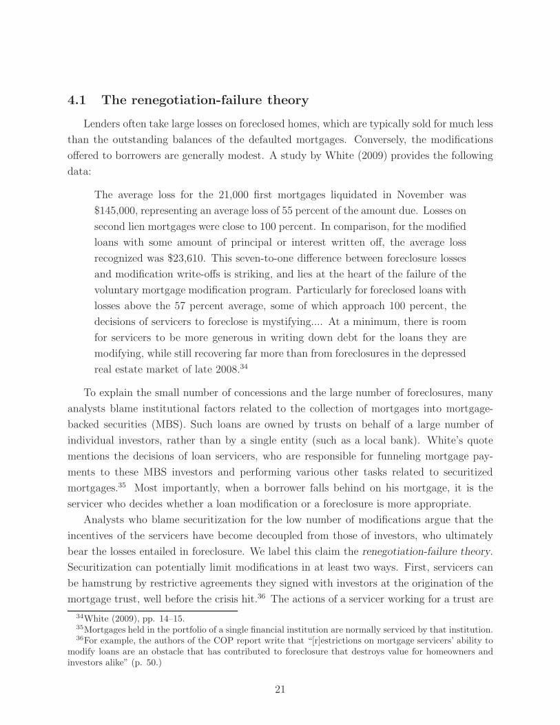
Lenders often take large losses on foreclosed homes, which are typically sold for much less

than the outstanding balances of the defaulted mortgages. Conversely, the modifications

offered to borrowers are generally modest. A study by White (2009) provides the following

data:

The average loss for the 21,000 first mortgages liquidated in November was

$145,000, representing an average loss of 55 percent of the amount due. Losses on

second lien mortgages were close to 100 percent. In comparison, for the modified

loans with some amount of principal or interest written off, the average loss

recognized was $23,610. This seven-to-one difference between foreclosure losses

and modification write-offs is striking, and lies at the heart of the failure of the

voluntary mortgage modification program. Particularly for foreclosed loans with

losses above the 57 percent average, some of which approach 100 percent, the

decisions of servicers to foreclose is mystifying.... At a minimum, there is room

for servicers to be more generous in writing down debt for the loans they are

modifying, while still recovering far more than from foreclosures in the depressed

real estate market of late 2008.34

To explain the small number of concessions and the large number of foreclosures, many

analysts blame institutional factors related to the collection of mortgages into mortgage-

backed securities (MBS). Such loans are owned by trusts on behalf of a large number of

individual investors, rather than by a single entity (such as a local bank). White’s quote

mentions the decisions of loan servicers, who are responsible for funneling mortgage pay-

ments to these MBS investors and performing various other tasks related to securitized

mortgages.35 Most importantly, when a borrower falls behind on his mortgage, it is the

servicer who decides whether a loan modification or a foreclosure is more appropriate.

Analysts who blame securitization for the low number of modifications argue that the

incentives of the servicers have become decoupled from those of investors, who ultimately

bear the losses entailed in foreclosure. We label this claim the renegotiation-failure theory.

Securitization can potentially limit modifications in at least two ways. First, servicers can

be hamstrung by restrictive agreements they signed with investors at the origination of the

mortgage trust, well before the crisis hit.36 The actions of a servicer working for a trust are

34White (2009), pp. 14–15.35Mortgages held in the portfolio of a single financial institution are normally serviced by that institution.36For example, the authors of the COP report write that “[r]estrictions on mortgage servicers’ ability to

modify loans are an obstacle that has contributed to foreclosure that destroys value for homeowners andinvestors alike” (p. 50.)

21

governed by so-called Pooling and Servicing Agreements (PSAs). Among other things, these

agreements specify the latitude that servicers have when deciding between modification and

foreclosure. As a general rule, PSAs allow servicers to make modifications, but only in cases

where default is likely and where the benefit of a modification over foreclosure can be shown

with a net-present-value (NPV) calculation. Second, proponents of the renegotiation-failure

theory claim that servicers are afraid that they will be sued by one tranche of investors

in the MBS if they make modifications, even if these modifications benefit the investors in

the trust as a whole. Because different tranches of investors have different claims to the

payment streams from the MBS, a modification may alter these streams in a way that will

benefit one tranche at the expense of another. One might think that the PSAs would have

foreseen this possibility, but some analysts claim that the PSAs were not written with an

eye to the current foreclosure crisis. Thus, it is claimed that there is enough ambiguity in

the PSAs to make servicers wary of getting caught up in “tranche warfare,” so servicers are

thought to follow the path of least resistance and foreclose on delinquent borrowers.37

A central implication of this theory is that securitization and the related frictions em-

bedded in the contracts between investors and servicers are preventing modifications that

would make even the lender better off. As Eggert (2007) states:

The complex webs that securitization weaves can be a trap and leave no one, not

even those who own the loans, able effectively to save borrowers from foreclosure.

With the loan sliced and tranched into so many separate interests, the different

claimants with their antagonistic rights may find it difficult to provide borrowers

with the necessary loan modifications, whether they want to or not (p. 292).38

4.2 Reasons to doubt the renegotiation-failure theory

There are, however, reasons to doubt the renegotiation-failure theory. First, there is

little evidence on the extent to which PSAs have limited modifications in practice.39 A 2007

study by Credit Suisse of approximately 30 PSAs concluded that fewer than 10 percent of

them completely ruled out modifications. About 40 percent of the PSAs allowed modifi-

cations, but with some restrictions. These restrictions included a limit on the percentage

37The authors of the COP report write that “[s]ervicers may also be reluctant to engage in more activeloan modification efforts because of litigation risk” (p. 46).

38Other policy analysts have adopted a similar view. For example, the COP writes in its recent reportthat “A series of impediments now block the negotiations that would bring together can-pay homeownerswith investors who hold their mortgages .... Because of these impediments, foreclosures that injure boththe investor and homeowner continue to mount” (COP report, p. 2).

39For a discussion of the role of PSAs in reducing modifications, see Cordell, Dynan, Lehnert, Liang, andMauskopf (2008), which also discusses the incentives faced by servicers more generally.

22

of mortgages in the pool that could be modified without permission from the trustee of

the mortgage-backed security (often 5 percent), and/or a floor for the mortgage rate that

could be applied in the event of a modification that entailed a reduction in the borrower’s

interest rate. The remainder of PSAs contained no restrictions. It is unlikely that even

PSAs with 5-percent caps are preventing modification to any significant degree. The Con-

gressional Oversight Panel for the Troubled Asset Recovery Program examined a number of

securitized pools with 5-percent caps and found that none had yet approached this cap.40

Moreover, one can make a case that the typical PSA actually compels the servicer to make

modifications if these modifications are in the best interests of the investor. According to

Cordell, Dynan, Lehnert, Liang, and Mauskopf (2008), “While investors seem somewhat

concerned about servicer capacity, they do not convey widespread concern that servicers

are relying overmuch on foreclosures relative to modifications.” In fact, investors opposed

additional incentives for modifications:

Investors with whom we spoke were not enthusiastic about an idea to reimburse

servicers for expenses of loss mitigation. In their view, such payments could

lead to more modifications than warranted by the NPV calculations. They also

felt that the PSA adequately specified that modifications that maximized NPV

should be undertaken. A typical response from an investor was, Why should I

pay servicers for doing something that I already paid them to do?41

Regarding the fear of lawsuits, no servicer has yet been sued for making too many loan

modifications. There has been a well-publicized lawsuit filed by a group of investors against

a servicer doing modifications, but the details of this suit should not make other servicers

wary about making modifications.42 Moreover, Hunt (2009) studied a number of subprime

securitization contracts and found not only that outright bans on modifications were rare,

but also that most contracts allowing modifications essentially instructed the servicer to

behave as if it were the single owner of the loan:

The most common rules [in making modifications] are that the servicer must

follow generally applicable servicing standards, service the loans in the interest

of the certificate holders and/or the trust, and service the loans as it would

40COP report (p. 44).41Cordell, Dynan, Lehnert, Liang, and Mauskopf (2008), p. 19.42Specifically, an MBS investor has sued two large servicers, Countrywide and Bank of America, for

promising to make mass modifications as part of a settlement that Countrywide and Bank of Americastruck with the government in a predatory lending case. The key argument by the investor in this lawsuitwas that the modifications were done not because they were profitable for the investors, but rather tosettle a predatory lending lawsuit, which the plaintiffs of that lawsuit claimed was the responsibility ofCountrywide, in its capacity as the originator of the troubled loans.

23

service loans held for its own portfolio. Notably, these conditions taken together

can be read as attempting to cause the loans to be serviced as if they had not

been securitized. (p. 8, insertion added)

The Hunt (2009) findings speak directly to whether the modification of securitized mort-

gages is analogous to the restructuring of troubled corporations, as has been suggested by

some economists. As was illustrated in negotiations over the recent Chrysler bankruptcy, a

single corporate bond holder can block a deal that is in the interests of all other stakeholders

in the firm.43 But any analogy between corporate bankruptcy and mortgage modification

is not appropriate. Not only can the typical mortgage servicer proceed with a modifica-

tion without the approval of all investors, the servicer does not need the approval of any

investor to modify a loan. Thus, there is no possibility of a hold-up problem. The authors

of the typical PSA appear to have anticipated the problems that could arise with dispersed

ownership, so the contract instructs the servicer to behave as if it alone owned the loan.

To preview our empirical results, we find that the data are consistent with the claim that

servicers are carefully following this type of contract.

While there can be substantial disagreement about the importance of any particular

institutional impediment to loan modification, perhaps the most compelling reason to be

skeptical about the renegotiation-failure theory is the sheer size of the losses it implies. We

can use White’s figures quoted above to come up with a back-of-the-envelope calculation for

the total losses that follow from the renegotiation-failure theory. One figure often cited for

the total number of foreclosures that can be prevented with modifications is 1.5 million.44

For a dollar figure, we can multiply this number of preventable foreclosures by the $120,000

that White claims is lost by investors for each foreclosure performed.45 This results in a

total deadweight loss of $180 billion.

Losses of this size may be hard to square with economic theory, as Eric Maskin recently

pointed out in a letter to the New York Times. Maskin wrote his letter in response to an

earlier op-ed that had claimed the government has a role in facilitating loan modifications,

specifically mass write-downs of principal balances.46 According to Maskin: “If, as claimed,

such write-downs are truly ‘win-win’ moves — allowing borrowers to keep their homes and

giving mortgage holders a higher return than foreclosure — they may not need the govern-

ment’s assistance.” The writers of the original op-ed column had claimed that servicers now

43See “A Chrysler Creditor Finds Himself Torn,” The Wall Street Journal, April 30, 2009.44This figure comes from FDIC Chairman Sheila Bair. For details see “Sheila Bair’s Mortgage Miracle,”

Wall Street Journal, December 3, 2008.45White (2008)46The op-ed to which Maskin responded is Geanakoplos and Koniak (2008). Maskin’s letter appeared on

March 7, 2009.

24

have an undue incentive to foreclose rather than modify loans. Maskin pointed out that if

this were the case, then

mortgage holders themselves have strong motivation to renegotiate those con-

tracts, so that the servicers’ incentives are corrected. That would be a win-win-

win move (for mortgage holders, servicers and borrowers), and to complete their

argument, the writers must show why it won’t happen.

Economists will recognize the reasoning in Maskin’s critique. The Coase Theorem implies

that economically efficient decisions will be made as long as property rights are well-defined

and transactions costs are not of first-order importance. Under these conditions, it does

not matter that servicers are not the ones who suffer the $180 billion losses entailed in

foreclosure, or even that existing PSAs might unduly limit modifications. The party that

suffers the potential losses — the investors — has an incentive to make side payments or

to change contractual arrangements so as to prevent these massive losses from occurring.

To take this reasoning one step further, if one class of investors has more to gain from

modification than another class stands to lose, the first class has an incentive to strike deals

with (or buy out) the second class. Consequently, to be consistent with the Coase Theorem,

the renegotiation-failure theory must also assert that the transactions costs implied by

securitization are large enough to derail these efficiency-enhancing arrangements, at the

cost to lenders of $180 billion.

4.3 A theory of loan modifications

There is another way to explain the low number of modifications that does not rely on

enormous transactions costs and yet is consistent with the Coase Theorem. It is simply

that most potential modifications are negative-NPV transactions from the standpoint of

investors. In other words, when all the relevant costs and benefits are considered, servicers

may already be acting in the best interests of the investors when they foreclose.47

To start with, modifications do not always prevent foreclosures, especially when defaults

are of the double-trigger variety. Consider a borrower who has lost his job. No permanent

modification can make the house affordable if the borrower has no income. Lenders often

offer “forbearance” in these cases, whereby the borrower pays sharply reduced payments

for a time. The borrower is then obligated to make up these arrears, with interest, later

on. Lenders may be reluctant to offer forbearance for any length of time if they are unsure

47Note that because of externalities from foreclosures, modifications may be in society’s interests even ifthey are not investors’ interests.

25

when the borrower will find a new job (and at what wage). When the value of the house

that collateralizes the loan is falling, and when all parties know that the house has probably

become unaffordable to the borrower, then the servicer may simply decide to take a loss

now by foreclosing, rather than risk an even larger loss down the road.48

The possibility that borrowers will re-default on their loans reduces the benefits of loan

modifications and thereby makes them less likely to occur. There are also reasons to think

that costs of modifications are higher than many housing analysts recognize. These analysts

typically ignore the costs of modifications that are made to borrowers who would have

repaid their loans anyway. Consider a lender facing a troubled borrower who is requesting

a modification. If the lender fails to modify the loan and the borrower defaults, the lender

will lose because (as White points out above), the cost of modifying the loan falls far short

of the cost of foreclosing. We will call this loss “Type I error.” However, Type I error is

only part of the story, as the lender faces another potential problem. If, unbeknownst to

the lender, the borrower requesting the modified loan will not default in the absence of a

modification, then the lender will lose the money he would have received according to the

original terms of the loan. We call this situation “Type II error.” For a modification to

make economic sense from the lender’s perspective, Type I error must exceed Type II error.

More formally, we can follow Foote, Gerardi, and Willen (2008), who consider a lender

with a borrower who owes m on a house currently worth pH dollars. This borrower will

default with probability α0, in which case the lender recovers pH less λ dollars in foreclosure

costs. A modification lowers the value of the loan to m∗ < m and the probability of

foreclosure to α1 < α0. Note that we do not assume that modification guarantees full

repayment of the mortgage — there is some probability of re-default when α1 > 0. Some

simple arithmetic shows that renegotiation occurs when:

Renegotiation ⇔ (α0 − α1)︸ ︷︷ ︸

Reduction in

foreclosure prob.

× (m∗ − (pH − λ))︸ ︷︷ ︸

Reduced

loss

> (1 − α0)︸ ︷︷ ︸

Pct. repay without

mitigation

× (m − m∗)︸ ︷︷ ︸

Reduced value of

the mortgage

. (3)

The first term corresponds to the Type I error — if a foreclosure is prevented, the lender

recovers m∗ rather than pH − λ. The second term corresponds to the Type II error —

borrowers who would have repaid in full, but take advantage of principal reduction to

reduce their debt burden.

48We have been told that there is a macabre saying in the servicing industry: “The first loss is the bestloss.”

26

The following reformulation of equation (3) is instructive:

m − m∗ <α0 − α1

1 − α1

[m − (pH − λ)]. (4)

The right-hand side is the maximum possible concession the lender can profitably make.

To understand this, consider some simple examples. If we set α0, the probability of default

without a modification, equal to 1, then equation (4) becomes

m∗ > pH − λ.

This is the case that White (2009) has in mind when he writes, “Particularly for foreclosed

loans with losses above the 57 percent average, some of which approach 100 percent, the

decisions of servicers to foreclose is mystifying.”49 In White’s extreme example of 100 percent

loss given default, even a modification that reduces the probability of default from 1 to

anything even infinitesimally less than one, and in which the lender recovers infinitesimally

more than 0, makes economic sense.

However, even a little uncertainty about whether the borrower will default invalidates

the above logic. If we assume modification ensures that the loan will repay with certainty

(α1 = 0), then equation (4) becomes:

m − m∗ < α0[m − (pH − λ)]. (5)

It is easy to see in this equation exactly how the math works against modification. Suppose

the expected loss is 57 percent and the likelihood of default is 50 percent, then the lender

can only reduce the value of the loan by 28.5 percent.

How big are Type I and Type II errors in practice? Results in Gerardi and Willen

(2009) show that for most categories of homeowners in Massachusetts, Type II is large

relative to Type I error: even with major stresses, most homeowners will not default on

their mortgages. The authors find that concessionary modifications make sense only for

multi-family properties purchased with subprime mortgages.

Equation (3) clearly illustrates that the observation that a foreclosure, on the surface,

seems to lead to greater monetary losses than an apparently reasonable modification is not

prima facie evidence of inefficiency. Such foreclosures may well be ex ante efficient, when the

issue of moral hazard is factored into the equation. This type of moral hazard explains why

mortgage investors are not unduly concerned about too few modifications being performed,

49White (2009), p. 15.

27

and why, to date, there have been no lawsuits against servicers encouraging them to do

more modifications.

4.4 Statistical evidence on loan modifications

The LPS data allow us to perform an econometric test of the renegotiation-failure theory,

because these data contain information on the ultimate holder (investor) of the residential

mortgages. Specifically, we are able to tell whether a mortgage is held on the balance sheet

of a financial institution, securitized by a government sponsored enterprise (GSE) such as

Freddie Mac (FHLMC) or Fannie Mae (FNMA), or securitized by a non-agency, private

institution. With this information, combined with information that allows us to identify

modified loans, we are able to compare the relative modification frequency between loans

held in portfolio and loans that are securitized. If institutional constraints inherent in the

securitization process are preventing profitable modifications, then we expect to see in the

data relatively few modifications among securitized loans, as compared with loans held in

portfolio.

The LPS dataset does not include direct information on loan modifications. However,

it does contain updated loan terms at a monthly frequency, with which we are able to

identify loan modifications indirectly (and imperfectly).50 With these data we label a loan

as modified if there is a change in its terms that was not stipulated by the initial terms of the

contract. These changes include interest-rate reductions, principal-balance reductions, and

term extensions. We can also identify principal-balance and mortgage-payment increases

that reflect the addition of arrears to the balance of a loan.51

Table 7 reports the number of modifications made by quarter from the first quarter of

2007 through the last quarter of 2008, disaggregated by the type of modification made.

Each of the numbers in the table is a multiple of 10 because we used a 10 percent random

sample and scaled up the numbers we found. The first column simply reports the total

50The Office of Thrift Supervision (OTS) and Office of the Comptroller of Currency (OCC) used verysimilar data from LPS to analyze the outcomes of recent mortgage modification programs (OCC and OTSMortgage Metrics Report, Third Quarter 2008) In their report, they used supplementary data directly fromlarge mortgage servicers that included the identification of loans in the LPS data that had been modified.While we do not have access to those data, our findings are fairly consistent with theirs.

51There are two potential mistakes we can make in this exercise. First, we may falsely identify modifica-tions (“false positives”) because of measurement error in the data (for example, a mistake in the updatedbalance or interest rate) or some endogenous behavior on the part of the borrower (for example, a borrowermaking extra principal payments). Second, we may miss modifications (“false negatives”) because our al-gorithm for finding modifications is incomplete. In this section we are more concerned with false positivesthan with false negatives, so we use a conservative set of criteria. See Adelino, Gerardi, and Willen (2009)for a detailed explanation of the exact algorithm used to identify modified loans in the LPS data.

28

number of loan modifications performed and shows that they have become more common

as the housing market has weakened. By our calculations, there appear to be more than

seven times as many modifications performed in the fourth quarter of 2008 as in the first

quarter of 2007.

In addition to the rapid growth in loan modifications, the composition of modifications

has changed over time. This can be seen in the remaining columns of Table 7, which list

the incidence of modifications of different types.52 A somewhat surprising finding is that

most modifications entailed increases in the principal balance of a mortgage. Such increases

are likely due to the addition of arrears to the outstanding mortgage balance for delinquent

borrowers, and they often increase the monthly mortgage payment by a nontrivial amount.

Table 7 shows that while the absolute numbers of balance-increasing modifications are still

rising, they are falling as a percentage of total modifications. In the last few quarters in our

data, interest-rate reductions, which necessarily involve a decrease in the mortgage payment,

have become more frequent, rising to more than 25 percent of all modifications performed

in 2008:Q4. Adelino, Gerardi, and Willen (2009) provide further information regarding

the behavior of monthly mortgage payments for loans that have undergone a modification.

The authors find that until the fourth quarter of 2008, modifications involving payment

increases were more common than those involving payment decreases. In addition, they find

that the average and median magnitudes of payment decreases have recently increased from

approximately 10–14 percent in the period between 2007:Q1 and 2008:Q2, to approximately

20 percent in the final two quarters of 2008. Based on the logic from our simple framework

above, it is likely that these will have more success than modifications involving increases

in the payment and/or balance.

Figure 8 contains some evidence from the LPS data to support this claim. The figure

contains Kaplan-Meier non-parametric, survival estimates (also known as the product limit

estimator) of the transition from modification to default.53 The figure considers a loan to

be in default when it becomes 90 days delinquent (approximately three missed payments).

52In many cases a mortgage will experience multiple types of modifications at the same time. For example,we see cases in the data in which the interest rate is decreased and at the same time the term of the loan isextended. Thus, the percentages in Table 7 are not calculated with respect to the number of loans modified,but rather with respect to the number of modifications performed.

53The Kaplan-Meier estimate of the survival function for delinquency is given by:

St =∏

ti<t

ni − mi

ni

, (6)

where S(t) is the probability that a borrower will not default through time t, di corresponds to the numberof loans that default at time ti, while ni corresponds to the number of loans that are “at-risk” of default attime ti, or in other words the number of loans that are still active and that have not defaulted before timeti.

29

The figure shows that modifications involving a decrease in the monthly payment are far

more successful than those involving an increase in the payment. For example, after one

year, the probability that a modified loan involving a payment increase becomes 90 days

delinquent is approximately 69 percent. In contrast, a modified loan involving a payment

decrease has a probability of becoming 90 days delinquent of approximately 52 percent.54 Of

course, it should be noted that the underlying data in Figure 8 come predominantly from

loan modifications that took place in 2007 and early-to-mid 2008, while the majority of

modifications in the LPS data occurred in the last two quarters of 2008. The Kaplan-Meier

estimator does account for right-censoring, but in order to draw more conclusive inferences

we will need to observe more data on these recent modifications. Another noteworthy

observation from Table 7 is that the incidence of principal reductions is extremely low

in our data. This is likely due to two factors. First, the LPS data under-represent the

subprime mortgage market.55 A few servicers that focus almost exclusively on subprime

mortgages have recently begun modification programs that involve principal reduction.56

In addition, from a theoretical perspective, principal reduction plans suffer from the severe

incomplete-information problem noted earlier. Balance reductions are appealing to both

borrowers in danger of default and those who are not. As a result, lenders have a strong

incentive to provide modifications only to those borrowers who are most likely to default.

Adelino, Gerardi, and Willen (2009) provide evidence to support this claim, as they show

that modified loans in the LPS dataset are characterized by high leverage, high initial debt-

to-income ratios, and low initial credit scores. These are the loans that are most likely to

default without a modification (that is, loans where α0 is high).

Table 8 contains modification statistics broken down by the holder of the mortgage. We

distinguish between mortgages held in portfolio, mortgages securitized by a GSE such as

Fannie Mae or Freddie Mac, and mortgages securitized by a private entity. For each quarter

of 2008, we calculate the percentage of loans outstanding at the beginning of each quarter

that were modified at some point in that quarter. Each panel in the table corresponds

to a different sample of mortgages. Panel A corresponds to all types of mortgages in the

data. Panel B corresponds to both subprime and Alt-A mortgages.57 Finally, each panel in

54The pattern is similar if we assume the more stringent definition of default, corresponding to thesituation in which foreclosure proceedings are initiated by the holder of the mortgage. In this case, modifiedloans involving a payment increase have a probability of experiencing a foreclosure of about 34 percent,while modifications involving a payment decrease have an associated probability of about 17 percent.

55The majority of subprime mortgages are securitized by non-agency firms, and for the period of interest,the LPS dataset includes approximately 35 percent of mortgages securitized by non-agency corporations.

56An October report by Credit Suisse notes that Ocwen Loan Servicing, LLC and Litton Loan Servic-ing LP were the only subprime servicers that had performed a nontrivial number of principal reductionmodifications. Neither of these servicers contribute to the LPS dataset.

57The definition of subprime and Alt-A comes directly from the servicers that contribute to the LPS

30

the table is disaggregated into three parts, corresponding to different denominators used in

calculating the percentages. The first part uses all loans outstanding at the beginning of the

respective quarter, the second part uses all loans that are 30 days delinquent at the start of

the respective quarter, and the third part uses all loans that are 60 days delinquent at the

start of the respective quarter. By limiting the sample to delinquent loans, we are partially

controlling for differences in credit quality between loans held in portfolio and loans that are

securitized. This control turns out to be important. In both of the panels, and in almost all

quarters, modifications for privately securitized loans are more frequent than for portfolio

loans when the relevant universe is the full sample of loans. However, privately securitized

loans are generally riskier than other loans, so this discrepancy may simply reflect the fact

that more privately securitized loans are in danger of foreclosure and are thus, candidates

for modification. When we narrow the focus to delinquent loans, the results become more

balanced. Portfolio loans have a slightly higher incidence of modification compared with

privately securitized in Panel A, while modifications are more common among portfolio

loans in many instances in Panel B (except in the fourth quarter of 2008).

There are at least two patterns of note in Table 8. First, while delinquent loans held

in portfolio appear to be modified more frequently than privately securitized mortgages

(except for subprime and Alt-A mortgages, as defined in the LPS data), the discrepancy

is not as large as it is often made out to be in policy circles and in media reports. For

the sample of all 30-day delinquent loans (Panel A) held in portfolio, 6.81 percent were

modified in the third quarter of 2008 and 8.55 percent in the fourth quarter of 2008. In

comparison, 6.28 percent and 6.23 percent of privately securitized mortgages were modified

in the third quarter and fourth quarter of 2008, respectively. We see similar, although

slightly larger discrepancies for 60-day delinquent loans, but in many instances the sign

changes for subprime and Alt-A loans (Panel B). The second take-away from the table

is that the GSEs appear to have been much more reluctant to modify loans, with the

exception of Freddie Mac in the third and fourth quarters of 2008. While the summary

statistics presented above suggest that the incidence of modification does not seem to be

greatly impeded by the process of securitization, there are a variety of factors that could be

contributing to the variation in Table 8, including substantial differences in characteristics

between portfolio-held loans and securitized loans. In addition, there may be significant lags

between the time when a loan becomes delinquent and the point when it is modified that are

not captured in Table 8. For example, if it were the case that the percentages of modified

loans were the same, but portfolio-held loans were modified more quickly than privately

securitized loans, Table 8 would show more portfolio-held loans being modified (since the

dataset. There is no additional distinction between subprime and Alt-A in the LPS dataset.

31

slower, privately securitized modifications would not be picked up in the table). For this

reason, a slightly more formal analysis is necessary, in which other observable differences

between securitized and portfolio loans are controlled for, and in which the timing issues

as well as right-censoring are also taken into account. Censoring is an especially important

problem, as there are currently many delinquent loans outstanding that are, or will soon

be, good candidates for modification, as the housing market continues to decline.

Figure 9 displays Kaplan-Meier estimates of the survival function with respect to the

transition from delinquency to modification, broken down by the holder of the mortgage.

While the Kaplan-Meier estimator does not control for other observable differences in mort-

gage characteristics, it does account for censoring and the timing issues discussed above.58

The figure contains two plots. The first plot displays estimates of the survival function

corresponding to the transition from 30 days delinquency (one mortgage payment behind)

to modification of all mortgages originated after 2004 in the LPS dataset, while the second

plot uses only data from subprime/Alt-A mortgages in the LPS data originated after 2004.

There are a few notable patterns contained in Figure 9. First, looking at the universe of

all mortgages, privately securitized loans and GNMA loans are more likely to have been

modified than loans held in portfolio and FNMA loans over a fairly long horizon. Condi-

tional on 30-day delinquency, a privately securitized loan has a 15 percent probability of

being modified after two years, and a 26 percent probability after three years, compared

with 11 percent and 16 percent for loans held in portfolio, respectively.59 Over a shorter

horizon, (less than one year), there is very little difference across different types of loans

when conditioning on 30-day delinquency. The patterns are slightly different for the sam-

ple of subprime/Alt-A loans, as the incidence of modification is virtually the same over all

horizons for portfolio-held and privately securitized loans.60

Before concluding our analysis of loan modifications, we take note of some other papers

that have examined the issue with the same data. Piskorski, Seru, and Vig (2009) find

that seriously delinquent portfolio loans in the LPS data are less likely to experience a

completed foreclosure than seriously delinquent securitized loans. The authors attribute

58Adelino, Gerardi, and Willen (2009) estimate Cox proportional hazard models of the transition fromdelinquency to modification, in which differences in observable loan and borrower characteristics are con-trolled for, and find results that support the patterns in Figure 9.

59These probabilities increase substantially for loans that become 60 days delinquent, but the relativepatterns are similar. Conditional on 60-day delinquency, a privately securitized loan has a 27 percentprobability of being modified after two years, and a 40 percent probability after three years, compared with23 percent and 32 percent for loans held in portfolio, respectively. See Adelino, Gerardi, and Willen (2009)for these plots.

60There are a trivial number of GNMA subprime loans in the data, and thus we drop GNMA from thegraph. In addition, there are only a small number of FNMA and FHLMC subprime loans that are seasonedbeyond two years, and thus we decided to truncate the graph for these types of loans after two years.

32

this finding to a greater willingness of portfolio lenders to modify loans, but a careful

analysis of the data does not support this inference. First, as we seen, portfolio lenders

are not more likely to modify mortgages.61 Portfolio lenders might be making “better”

modifications than servicers of securitized loans, which could in theory explain the smaller

number of foreclosures among delinquent portfolio loans. However, Adelino, Gerardi, and

Willen (2009) show that the sheer number of modifications among all types of seriously

delinquent loans (about 7 percent) is far too low for differences in modification quality to

explain Piskorski et al.’s findings. A second issue stems from Piskorski et al.’s use of a

completed foreclosure as the relevant loan outcome. If portfolio lenders were truly more

willing to modify, as Piskorski et al. claim, then we would expect not only fewer bad

outcomes among portfolio loans (that is, fewer foreclosures), but also more good outcomes

(for example, more transitions to current status or to prepayment). After all, servicers

immediately classify modified loans as current. But Adelino et al. also show that delinquent

portfolio loans are no more likely to transition to current or prepaid status than securitized

loans.62 All told, the likely explanation for the Piskorski et al. finding of fewer foreclosures

among delinquent portolio loans is not a higher willingness of portfolio lenders to modify

loans, but rather various accounting and regulatory issues that make portfolio servicers less

willing to complete the foreclosure process.

4.5 Historical evidence on loan modifications

In addition to comparing securitized vs. non-securitized loans today, we can evaluate

claims about contract-related frictions by looking at the historical record. It is often claimed

that renegotiation was frequent in the past, before securitized mortgages were common. For

example, a report from the Congressional Oversight Panel for the Troubled Asset Recovery

Program states that

For decades, lenders in this circumstance could negotiate with can-pay borrowers

to maximize the value of the loan for the lender (100 percent of the market value)

and for the homeowner (a sustainable mortgage that lets the family stay in the

home). Because the lender held the mortgage and bore all the loss if the family

couldn’t pay, it had every incentive to work something out if a repayment was

61The Piskorski et al. paper never tries to identify modifications directly, as we do.62This finding may seem inconsistent with the reduced likelihood of completed foreclosures among portfolio

loans. But a complicating fact is that most of the loan data is right-censored. The difference in completedforeclosures is offset by an increased number of loans that are more than 90 days delinquent or in somestage of foreclosure when the data is truncated.

33

possible.63

Other authors, including Zingales (2008) and Geanakoplos and Koniak (2008), have also

claimed that renegotiation used to be common, but we know of no historical studies that

verify this claim. There are, however, reasons to be skeptical. First, foreclosures were quite

common in the past. Between 1929 and 1936, lenders carried out 1.8 million foreclosures

in the United States. To put that number in perspective, keep in mind that the number

of occupied dwellings more than quadrupled from 22.9 million in 1930 to 105 million in

2000.64 In addition, increases in credit and increases in owner-occupancy have resulted

in the number of owner-occupied, mortgaged homes rising from 4.8 million in 1940 to 39

million in 2000. Thus, an equivalent figure for the current crisis would be between 8.3 and

17 million foreclosures.

Another way to compare foreclosures in the current era with foreclosures during the

Depression is to the look at the performance of vintages of loans. The top panel of Figure

10 shows the fraction of loans foreclosed upon by year of origination for the three prin-

cipal sources of credit in that period: savings and loan institutions (S&L), life insurance

companies, and commercial banks. The worst vintages were those of the late 1920s, when

approximately 30 percent of loans originated by life insurance companies ended in foreclo-

sure, 20 percent of S&L mortgages ended in foreclosure, and about 15 percent of commercial

bank loans were foreclosed upon. The bottom panel shows the fraction of homeownerships

(not loans) originated each year in Massachusetts from 1988 through 2008 that eventually

ended in foreclosure.65 Since at least some of these foreclosures did not occur on purchase

mortgages, but rather on subsequent refinances, one can view this as an upper bound on a

similar measure using current data. What is clear is that we see far fewer foreclosures than

we did in the 1930s. These statistics are difficult to square with the claim that renegotiation

was more common in the past.

In fact, historical documents do suggest that modifications occurred in the past. The

Home Owners Loan Corporation (HOLC), set up by the federal government in 1933 in

the midst of the Great Depression, would buy loans at a deep discount from lenders and

re-underwrite the borrower into a new mortgage consistent with the borrower’s financial

situation at the time. However, it is important to understand that the economic situation

was extremely poor, as 40 percent of American homeowners were more than 15 months in

arrears. In terms of our model, this made Type I error large and Type II error small.66

63COP report, p. 2.64Source: U.S. Census of Housing, 2000, Table DP-4, and 1950, Part 1, Table J.65See Gerardi, Shapiro, and Willen (2007) for details regarding the Massachusetts data.66See Harriss (1951) for details about HOLC.

34

Unfortunately, we do not have detailed data on the subsequent mortgages to analyze the

ultimate experiences of HOLC borrowers.

In addition, commercial banks commonly modified loans in this time period. Behrens

(1952) shows that as many as 40 percent of the loans originated in a given year would

be modified at least once, and as many as half of those more than once. However, it is

important to understand that until the 1930s, commercial banks could not make long-term

amortized loans, so renegotiation for term extensions and interest rate changes was common.

According to Behrens, “It should also be observed that the low level of interest rates current

in the 1930s as compared with that prevailing during the 1920s doubtless stimulated a good

many of the loan modifications, primarily for those loans in good standing...”

In general, discussions of foreclosure from contemporary sources in “past decades” never

mention concessionary modification as a strategy for dealing with troubled borrowers. A

book on what we would now call “best practices” in mortgage banking, written in the

mid-1950s, gives a detailed discussion of how to contact delinquent borrowers, but then

recommends turning the problem over to an attorney.67 The author then discusses how to

deal with the sale of a foreclosed property but never suggests that the servicer should make

concessions to help the borrower continue making payments. Even HOLC, to a large extent,

considered mostly non-concessionary modifications and foreclosed on almost 20 percent of

the borrowers to whom it lent.68

Foreclosure has always been a common outcome in mortgage lending, even for the best-

intentioned of lenders. The first borrower ever to obtain a loan from a Building and Loan

Society in the U.S. was eventually forced out of his home. A man named Comly Rich took

out a mortgage on April 11, 1831, but “was frequently fined for failure to pay his dues and

interest.” The problems were resolved in what amounts to a foreclosure: both the house and

the mortgage were transferred to another borrower.69

5 Conclusion

In this paper, we have attempted to make two main points. First, while the concept

of mortgage “affordability” is often used in explanations of the current rise in mortgage

defaults, this concept is not helpful if it is not defined precisely. Many people believe

that the affordability of a mortgage is adequately summarized in the DTI at origination.

However, this ratio does not appear to be a strong predictor of default. What really matters

67Pease and Cherrington (1953).68Harriss (1951).69See Bodfish (1931), pp. 66–72.

35

in the default decision is the mortgage payment relative to the borrower’s income in the

present and future, not the borrower’s income in the past. Consequently, the high degree

of volatility in individual incomes means that mortgages that start out with low DTIs can

end in default if housing prices are falling. A second, related point concerns the apparent

unwillingness of loan servicers to turn “bad” (that is, high-DTI) mortgages into “good”

(low-DTI) mortgages. It is true that lenders may lose a great deal of money with each

individual foreclosure, but the loan modifications might have negative NPV if they are

sometimes extended to people who are likely to pay on time anyway. And the benefits of

modifications are uncertain if borrowers have lost their jobs.

What do these findings suggest for foreclosure-reduction policy? One suggestion would

be to focus a program on the effects of income volatility, helping people who lose their

jobs get through difficult periods without having to leave their homes. For example, the

government could replace a portion of lost income for a period of one or two years, through a

program of loans or grants to individual homeowners.70 For more permanent and very large

setbacks, the government could help homeowners transition to rentership through short sales

or other procedures. Whatever policies are adopted, the results of this paper suggest that

policies that encourage moderate, long-term reductions in DTIs face important hurdles in

addressing the current foreclosure crisis.

70For details of such a plan, see http://bosfed.org/economic/paymentsharingproposal.pdf.

36

References

Adelino, M., K. Gerardi, and P. S. Willen (2009). Renegotiating Home Mortgages: Evi-

dence from the Subprime Mortgage Crisis. Working Paper .

Behrens, C. F. (1952). Commercial Bank Activities in Urban Mortgage Financing. New

York, NY: National Bureau of Economic Research.

Bodfish, H. M. (1931). History of Building and Loan in the United States. Chicago, IL:

United States Building and Loan League.

Congressional Oversight Panel of the Troubled Assets Recovery Program (COP) (2009).

Foreclosure Crisis: Working Toward A Solution.

Cordell, L., K. Dynan, A. Lehnert, N. Liang, and E. Mauskopf (2008). The Incentives of

Mortgage Servicers: Myths and Realities. Finance and Economics Discussion Series,

Federal Reserve Board 46.

Cordell, L., M. Watson, and J. Thomson (2008). McDash Data Warehouse Seminar.

Danis, M. A. and A. N. Pennington-Cross (2005). The Delinquency of Subprime Mort-

gages. SSRN eLibrary .

Dell’Ariccia, G., D. Igan, and L. Laeven (2009). Credit booms and lending standards:

Evidence from the subprime mortgage market.

Deng, Y., J. Quigley, and R. V. Order (2000). Mortgage terminations, heterogeneity and

the exercise of mortgage options. Econometrica 68 (2), 275–307.

Eggert, K. (2007). Comment on Michael A. Stegman et al.’s “Preventive Servicing Is Good

for Business and Affordable Homeownership Policy”: What Prevents Loan Modifica-

tions. Housing Policy Debate 18 (2), 279–297.

Foote, C., K. Gerardi, L. Goette, and P. S. Willen (2008). Just the facts: An initial

analysis of subprime’s role in the housing crisis. Journal of Housing Economics 17 (4),

1–24.

Foote, C., K. Gerardi, and P. Willen (2008). Negative equity and foreclosure: Theory and

evidence. Journal of Urban Economics 6 (2), 234–245.

Geanakoplos, J. and S. Koniak (2008). The best way to help homeowners – and the

economy. Available at http://cowles.econ.yale.edu/gean/crisis/index.htm.

Gerardi, K., A. Shapiro, and P. Willen (2007). Subprime outcomes: Risky mortgages,

homeownership experiences, and foreclosures. Federal Reserve Bank of Boston Work-

ing Paper 07-15.

37

Gerardi, K. and P. Willen (2009). Subprime Mortgages, Foreclosures and Urban Neigh-

borhoods. The B.E. Journal of Economic Analysis & Policy 9 (3 (Symposium)).

Gourinchas, P. and J. Parker (2002). Consumption over the life cycle. Econometrica,

47–89.

Harnick, E. (2009). Examining the Making Home Affordable Program, Testimony Before

the U.S. House of Representatives Committee on Financial Services, Subcommittee

on Housing and Community Opportunity.

Harriss, C. L. (1951). History and Policies of the Home Owners’ Loan Corporation. New

York, NY: National Bureau of Economic Research.

Himmelberg, C., C. Mayer, and T. Sinai (2005). Assessing high house prices: bubbles,

fundamentals and misperceptions. Journal of Economic Perspectives 19 (4), 67–92.

Hunt, J. (2009). What do subprime securitization contracts actually say about loan mod-

ification. Berkeley Center for Law, Business and the Economy.

Kau, J. B., D. C. Keenan, and T. Kim (1994). Default probabilities for mortgages. Journal

of Urban Economics 35 (3), 278–296.

Kiefer, N. (1988). Economic duration data and hazard functions. Journal of economic

literature, 646–679.

Mayer, C. J. and K. Pence (2008, June). Subprime mortgages: What, where, and to

whom? Working Paper 14083, National Bureau of Economic Research.

Mian, A. R. and A. Sufi (2009). The Consequences of Mortgage Credit Expansion: Evi-

dence from the U.S. Mortgage Default Crisis. Quarterly Journal of Economics forth-

coming.

Morton, J. E. (Ed.) (1956). Urban Mortgage Lending: Comparative Markets and Experi-

ence. New York, NY: National Bureau of Economic Research.

Pease, R. H. and H. V. Cherrington (Eds.) (1953). Mortgage Banking. New York, NY:

McGraw-Hill.

Piskorski, T., A. Seru, and V. Vig (2009). Securitization and Distressed Loan Renegoti-

ation: Evidence from the Subprime Mortgage Crisis.

Poterba, J. (1984). Tax subsidies to owner-occupied housing: an asset-market approach.

The Quarterly Journal of Economics, 729–752.

Sherlund, S. (2008). The past, present, and future of subprime mortgages. Finance and

Economics Discussion Series 2008-63, Federal Reserve Board.

38

White, A. M. (2008). Rewriting Contracts, Wholesale: Data on Voluntary Mortgage

Modifications from 2007 and 2008 Remittance Reports. Fordham Urban Law Jour-

nal forthcoming.

White, A. M. (2009). Deleveraging the American Homeowner: The Failure of 2008 Vol-

untary Mortgage Contract Modifications. Connecticut Law Review forthcoming.

Zingales, L. (2008). Plan b. Economists’ Voice 5 (6), 4.

39

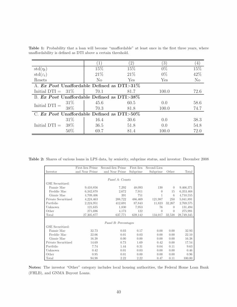
Table 1: Probability that a loan will become “unaffordable” at least once in the first three years, whereunaffordability is defined as DTI above a certain threshold.

(1) (2) (3) (4)std(ηt) 15% 15% 0% 15%std(εt) 21% 21% 0% 42%Resets No Yes Yes NoA. Ex Post Unaffordable Defined as DTI>31%

Initial DTI = 31% 70.1 81.7 100.0 72.6B. Ex Post Unaffordable Defined as DTI>38%

Initial DTI =31% 45.6 60.5 0.0 58.638% 70.3 81.8 100.0 74.7

C. Ex Post Unaffordable Defined as DTI>50%

Initial DTI =31% 16.4 30.6 0.0 38.338% 36.5 51.8 0.0 54.850% 69.7 81.4 100.0 72.0

Table 2: Shares of various loans in LPS data, by seniority, subprime status, and investor: December 2008

First-lien Prime Second-lien Prime First-lien Second-LienInvestor and Near Prime and Near Prime Subprime Subprime Other Total

Panel A: Counts

GSE Securitized:Fannie Mae 9,410,856 7,292 48,093 130 0 9,466,371Freddie Mac 6,342,870 2,672 7,911 0 15 6,353,468Ginnie Mae 4,709,406 391 751 1 6 4,710,555

Private Securitized 4,224,463 208,722 486,469 121,987 250 5,041,891Portfolio 2,224,951 412,691 87,843 11,823 32,267 2,769,575Unknown 121,635 1,830 7,953 76 0 131,494Other 271,696 4,173 122 0 0 275,991Total 27,305,877 637,771 639,142 134,017 32,538 28,749,345

Panel B: Percentages

GSE Securitized:Fannie Mae 32.73 0.03 0.17 0.00 0.00 32.93Freddie Mac 22.06 0.01 0.03 0.00 0.00 22.10Ginnie Mae 16.38 0.00 0.00 0.00 0.00 16.38

Private Securitized 14.69 0.73 1.69 0.42 0.00 17.54Portfolio 7.74 1.44 0.31 0.04 0.11 9.63Unknown 0.42 0.01 0.03 0.00 0.00 0.46Other 0.95 0.01 0.00 0.00 0.00 0.96Total 94.98 2.22 2.22 0.47 0.11 100.00

Notes: The investor “Other” category includes local housing authorities, the Federal Home Loan Bank

(FHLB), and GNMA Buyout Loans.

40

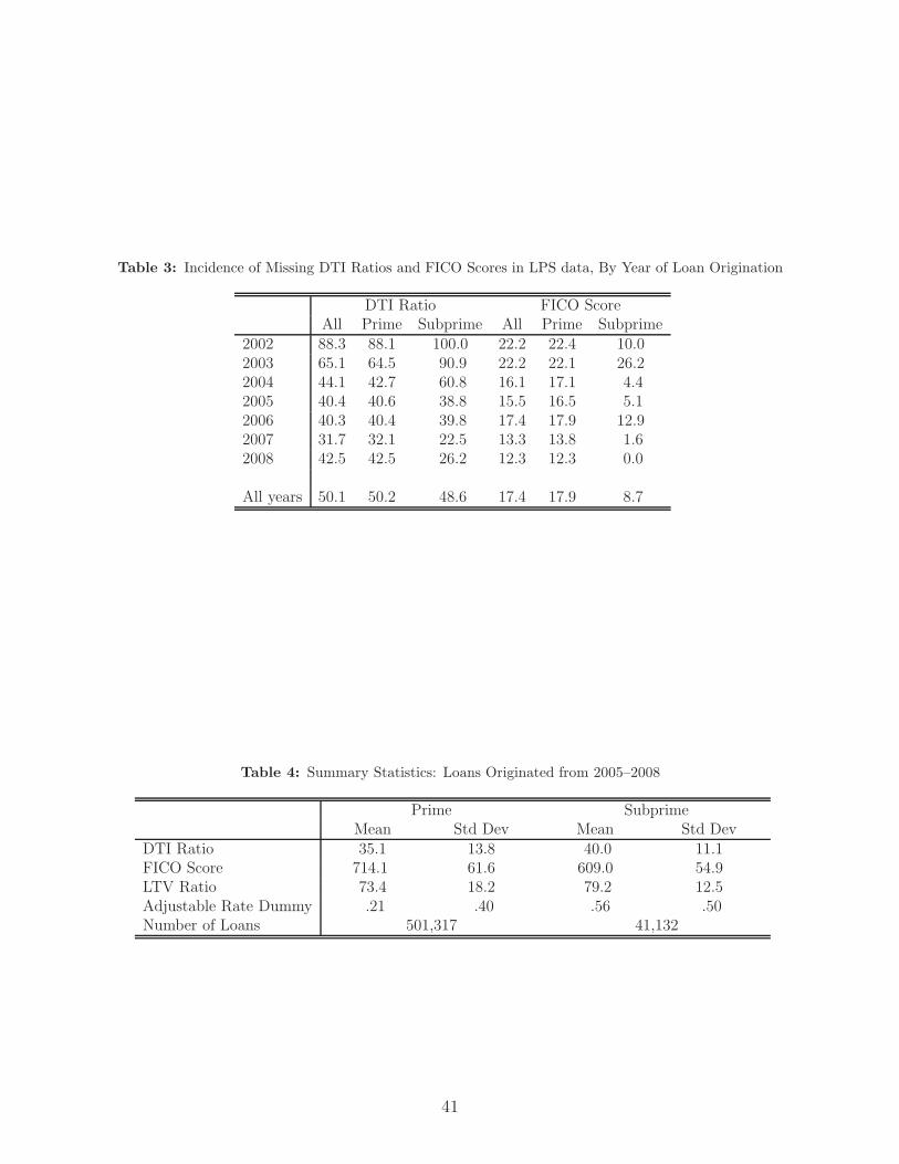
Table 3: Incidence of Missing DTI Ratios and FICO Scores in LPS data, By Year of Loan Origination

DTI Ratio FICO ScoreAll Prime Subprime All Prime Subprime

2002 88.3 88.1 100.0 22.2 22.4 10.02003 65.1 64.5 90.9 22.2 22.1 26.22004 44.1 42.7 60.8 16.1 17.1 4.42005 40.4 40.6 38.8 15.5 16.5 5.12006 40.3 40.4 39.8 17.4 17.9 12.92007 31.7 32.1 22.5 13.3 13.8 1.62008 42.5 42.5 26.2 12.3 12.3 0.0

All years 50.1 50.2 48.6 17.4 17.9 8.7

Table 4: Summary Statistics: Loans Originated from 2005–2008

Prime SubprimeMean Std Dev Mean Std Dev

DTI Ratio 35.1 13.8 40.0 11.1FICO Score 714.1 61.6 609.0 54.9LTV Ratio 73.4 18.2 79.2 12.5Adjustable Rate Dummy .21 .40 .56 .50Number of Loans 501,317 41,132

41

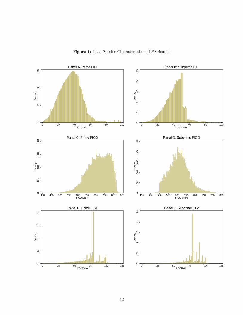
Figure 1: Loan-Specific Characteristics in LPS Sample

0.0

1.0

2.0

3D

ensi

ty

0 20 40 60 80 100DTI Ratio

Panel A: Prime DTI

0.0

1.0

2.0

3.0

4.0

5D

ensi

ty

0 20 40 60 80 100DTI Ratio

Panel B: Subprime DTI

0.0

02.0

04.0

06.0

08D

ensi

ty

400 450 500 550 600 650 700 750 800 850FICO Score

Panel C: Prime FICO0

.002

.004

.006

.008

.01

Den

sity

400 450 500 550 600 650 700 750 800 850FICO Score

Panel D: Subprime FICO

0.0

5.1

.15

.2D

ensi

ty

0 25 50 75 100 125LTV Ratio

Panel E: Prime LTV

0.0

5.1

.15

.2.2

5D

ensi

ty

0 25 50 75 100 125LTV Ratio

Panel F: Subprime LTV

42

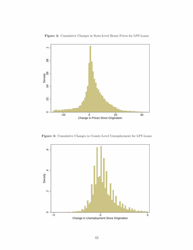
Figure 2: Cumulative Changes in State-Level House Prices for LPS Loans

0.0

2.0

4.0

6.0

8.1

Den

sity

−20 0 20 40Change in Prices Since Origination

Figure 3: Cumulative Changes in County-Level Unemployment for LPS Loans

0.2

.4.6

Den

sity

−5 0 5Change in Unemployment Since Origination

43

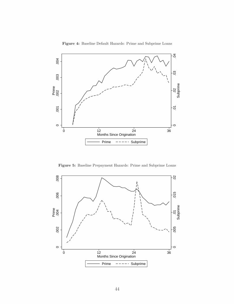
Figure 4: Baseline Default Hazards: Prime and Subprime Loans

0.0

1.0

2.0

3.0

4S

ubpr

ime

0.0

01.0

02.0

03.0

04P

rime

0 12 24 36Months Since Origination

Prime Subprime

Figure 5: Baseline Prepayment Hazards: Prime and Subprime Loans

0.0

05.0

1.0

15.0

2S

ubpr

ime

0.0

02.0

04.0

06.0

08P

rime

0 12 24 36Months Since Origination

Prime Subprime

44

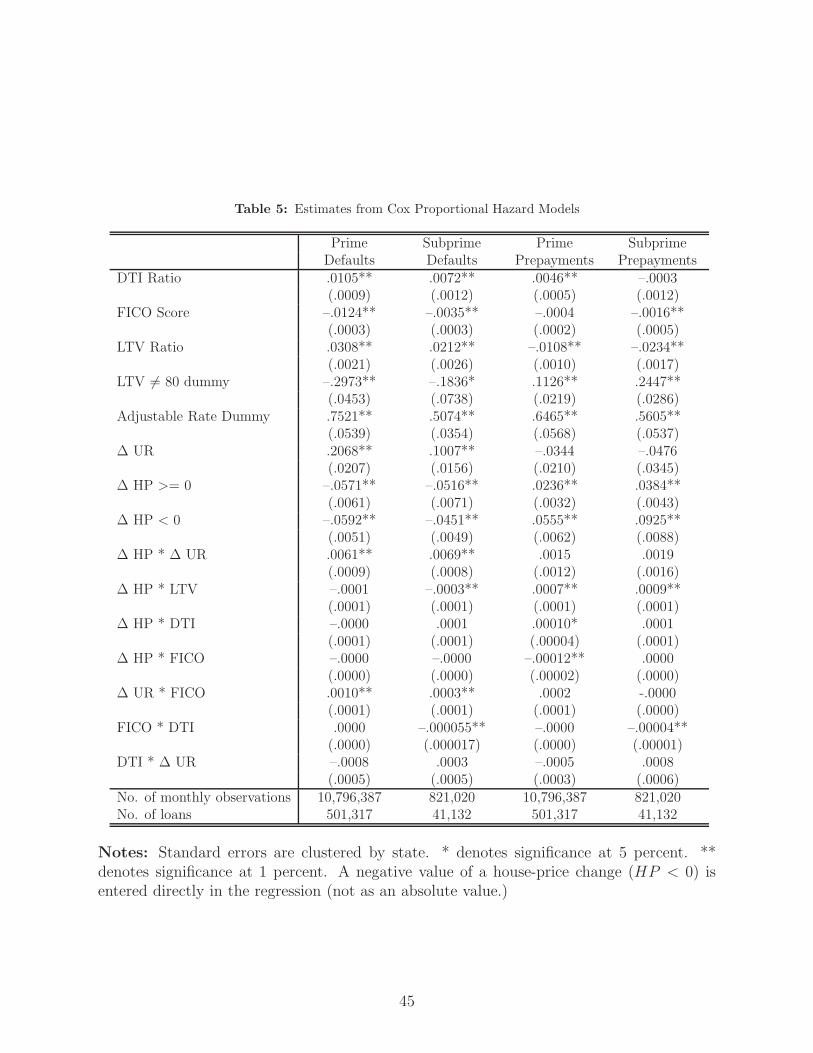
Table 5: Estimates from Cox Proportional Hazard Models

Prime Subprime Prime SubprimeDefaults Defaults Prepayments Prepayments

DTI Ratio .0105** .0072** .0046** –.0003(.0009) (.0012) (.0005) (.0012)

FICO Score –.0124** –.0035** –.0004 –.0016**(.0003) (.0003) (.0002) (.0005)

LTV Ratio .0308** .0212** –.0108** –.0234**(.0021) (.0026) (.0010) (.0017)

LTV 6= 80 dummy –.2973** –.1836* .1126** .2447**(.0453) (.0738) (.0219) (.0286)

Adjustable Rate Dummy .7521** .5074** .6465** .5605**(.0539) (.0354) (.0568) (.0537)

∆ UR .2068** .1007** –.0344 –.0476(.0207) (.0156) (.0210) (.0345)

∆ HP >= 0 –.0571** –.0516** .0236** .0384**(.0061) (.0071) (.0032) (.0043)

∆ HP < 0 –.0592** –.0451** .0555** .0925**(.0051) (.0049) (.0062) (.0088)

∆ HP * ∆ UR .0061** .0069** .0015 .0019(.0009) (.0008) (.0012) (.0016)

∆ HP * LTV –.0001 –.0003** .0007** .0009**(.0001) (.0001) (.0001) (.0001)

∆ HP * DTI –.0000 .0001 .00010* .0001(.0001) (.0001) (.00004) (.0001)

∆ HP * FICO –.0000 –.0000 –.00012** .0000(.0000) (.0000) (.00002) (.0000)

∆ UR * FICO .0010** .0003** .0002 -.0000(.0001) (.0001) (.0001) (.0000)

FICO * DTI .0000 –.000055** –.0000 –.00004**(.0000) (.000017) (.0000) (.00001)

DTI * ∆ UR –.0008 .0003 –.0005 .0008(.0005) (.0005) (.0003) (.0006)

No. of monthly observations 10,796,387 821,020 10,796,387 821,020No. of loans 501,317 41,132 501,317 41,132

Notes: Standard errors are clustered by state. * denotes significance at 5 percent. **denotes significance at 1 percent. A negative value of a house-price change (HP < 0) isentered directly in the regression (not as an absolute value.)

45

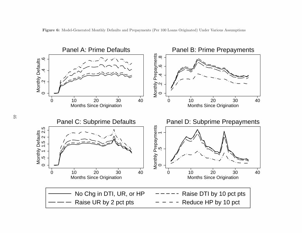
Figure 6: Model-Generated Monthly Defaults and Prepayments (Per 100 Loans Originated) Under Various Assumptions

0.2

.4.6

Mon

thly

Def

aults

0 10 20 30 40Months Since Origination

Panel A: Prime Defaults

0.2

.4.6

.8M

onth

ly P

repa

ymen

ts

0 10 20 30 40Months Since Origination

Panel B: Prime Prepayments0

.51

1.5

22.

5M

onth

ly D

efau

lts

0 10 20 30 40Months Since Origination

Panel C: Subprime Defaults

0.5

1M

onth

ly P

repa

ymen

ts

0 10 20 30 40Months Since Origination

Panel D: Subprime Prepayments

No Chg in DTI, UR, or HP Raise DTI by 10 pct ptsRaise UR by 2 pct pts Reduce HP by 10 pct

46

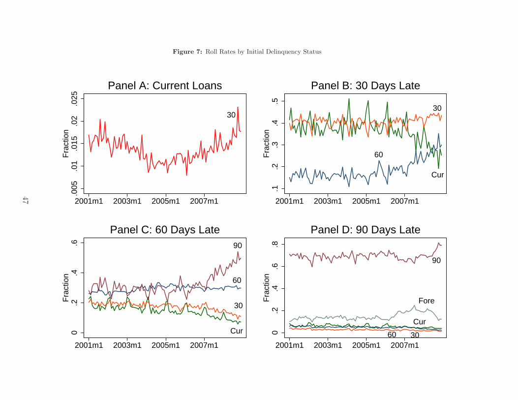
Figure 7: Roll Rates by Initial Delinquency Status

30

.005

.01

.015

.02

.025

Fra

ctio

n

2001m1 2003m1 2005m1 2007m1

Panel A: Current Loans

30

60

Cur

.1.2

.3.4

.5F

ract

ion

2001m1 2003m1 2005m1 2007m1

Panel B: 30 Days Late

90

60

30

Cur0.2

.4.6

Fra

ctio

n

2001m1 2003m1 2005m1 2007m1

Panel C: 60 Days Late

90

Fore

3060

Cur

0.2

.4.6

.8F

ract

ion

2001m1 2003m1 2005m1 2007m1

Panel D: 90 Days Late

47

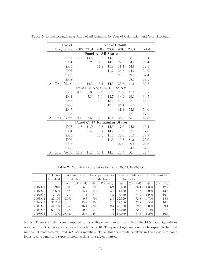
Table 6: Direct Defaults as a Share of All Defaults, by Year of Origination and Year of Default

Year of Year of DefaultOrigination 2003 2004 2005 2006 2007 2008 Total

Panel A: All States

2003 11.4 10.8 15.3 14.1 18.0 28.1 16.42004 8.2 12.5 14.5 22.7 34.4 20.42005 11.2 15.8 31.4 44.6 32.12006 11.7 25.7 44.0 34.92007 25.5 39.7 37.42008 38.1 38.1

All Orig. Years 11.4 10.3 13.1 14.5 26.6 41.6 30.8Panel B: AZ, CA, FL, & NV

2003 9.4 5.0 5.4 8.7 20.9 41.0 16.82004 7.3 6.6 13.7 33.9 49.3 30.52005 5.0 18.1 43.9 57.7 46.22006 12.5 34.4 55.8 46.52007 31.3 53.9 50.62008 47.1 47.1

All Orig. Years 9.4 5.5 6.0 15.4 36.8 55.1 44.8Panel C: 47 Remaining States

2003 11.8 11.9 16.3 14.6 17.6 24.9 16.42004 8.4 13.4 14.7 19.9 27.3 17.82005 12.6 15.0 23.0 31.5 22.92006 11.3 19.8 31.6 25.02007 22.0 29.6 28.32008 34.5 34.5

All Orig. Years 11.8 11.2 14.1 14.3 20.7 30.4 22.7

Table 7: Modification Statistics by Type: 2007:Q1–2008:Q4

# Loans Interest Rate Principal Balance Principal Balance Term ExtensionsModified Reductions Reductions Increases

# (% total) # (% total) # (% total) # (% total)2007:Q1 10,940 600 5.3 700 6.2 8,660 76.4 1,380 12.22007:Q2 14,600 820 5.4 550 3.7 11,630 77.3 2,050 13.62007:Q3 17,720 770 4.1 810 4.3 15,170 81.2 1,940 10.42007:Q4 27,150 2,990 9.7 700 2.3 22,520 72.8 4,740 15.32008:Q1 36,230 6,010 13.8 900 2.1 32,100 73.8 4,500 10.32008:Q2 44,750 9,050 16.4 1,300 2.4 39,750 72.1 5,030 9.12008:Q3 62,190 16,280 20.3 940 1.2 56,940 70.9 6,110 7.62008:Q4 74,800 28,630 26.7 1,450 1.4 65,960 61.5 11,230 10.5

Notes: These statistics were computed using a 10 percent random sample of the LPS data. Quantities

obtained from the data are multiplied by a factor of 10. The percentages are taken with respect to the total

number of modifications, and not loans modified. Thus, there is double-counting in the sense that some

loans received multiple types of modifications in a given quarter.

48

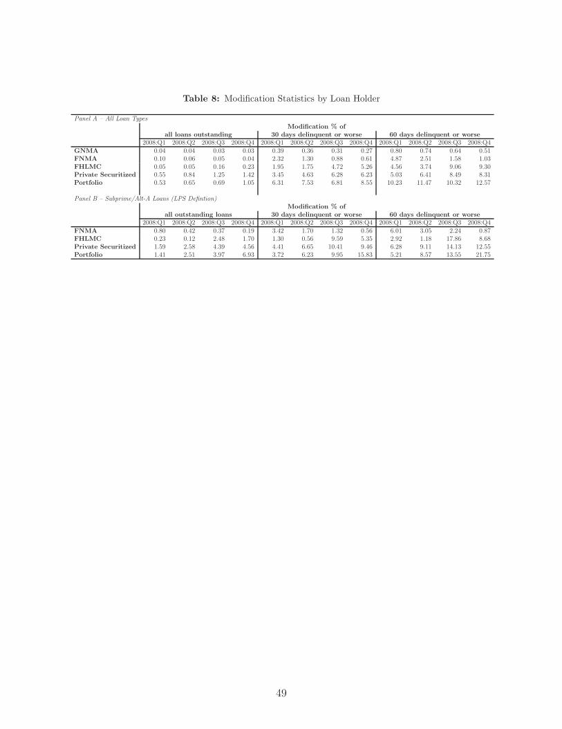
Table 8: Modification Statistics by Loan Holder

Panel A – All Loan TypesModification % of

all loans outstanding 30 days delinquent or worse 60 days delinquent or worse

2008:Q1 2008:Q2 2008:Q3 2008:Q4 2008:Q1 2008:Q2 2008:Q3 2008:Q4 2008:Q1 2008:Q2 2008:Q3 2008:Q4GNMA 0.04 0.04 0.03 0.03 0.39 0.36 0.31 0.27 0.80 0.74 0.64 0.51FNMA 0.10 0.06 0.05 0.04 2.32 1.30 0.88 0.61 4.87 2.51 1.58 1.03FHLMC 0.05 0.05 0.16 0.23 1.95 1.75 4.72 5.26 4.56 3.74 9.06 9.30Private Securitized 0.55 0.84 1.25 1.42 3.45 4.63 6.28 6.23 5.03 6.41 8.49 8.31Portfolio 0.53 0.65 0.69 1.05 6.31 7.53 6.81 8.55 10.23 11.47 10.32 12.57

Panel B – Subprime/Alt-A Loans (LPS Defintion)Modification % of

all outstanding loans 30 days delinquent or worse 60 days delinquent or worse

2008:Q1 2008:Q2 2008:Q3 2008:Q4 2008:Q1 2008:Q2 2008:Q3 2008:Q4 2008:Q1 2008:Q2 2008:Q3 2008:Q4FNMA 0.80 0.42 0.37 0.19 3.42 1.70 1.32 0.56 6.01 3.05 2.24 0.87FHLMC 0.23 0.12 2.48 1.70 1.30 0.56 9.59 5.35 2.92 1.18 17.86 8.68Private Securitized 1.59 2.58 4.39 4.56 4.41 6.65 10.41 9.46 6.28 9.11 14.13 12.55Portfolio 1.41 2.51 3.97 6.93 3.72 6.23 9.95 15.83 5.21 8.57 13.55 21.75

49

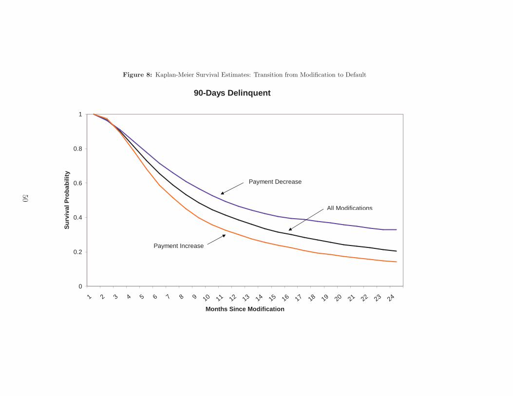
Figure 8: Kaplan-Meier Survival Estimates: Transition from Modification to Default

90-Days Delinquent

0

0.2

0.4

0.6

0.8

1

1 2 3 4 5 6 7 8 9 10 11 12 13 14 15 16 17 18 19 20 21 22 23 24

Months Since Modification

Su

rviv

al P

rob

abili

ty

Payment Decrease

Payment Increase

All Modifications

50

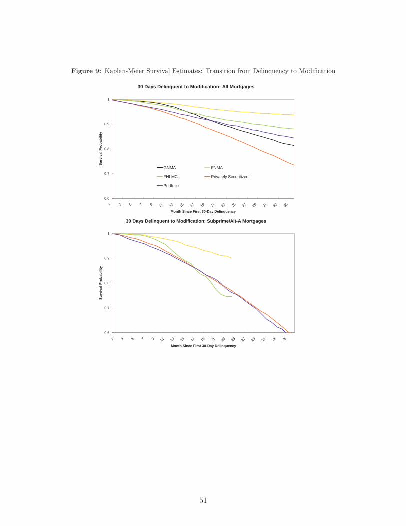
Figure 9: Kaplan-Meier Survival Estimates: Transition from Delinquency to Modification

30 Days Delinquent to Modification: All Mortgages

0.6

0.7

0.8

0.9

1

1 3 5 7 9 11 13 15 17 19 21 23 25 27 29 31 33 35

Month Since First 30-Day Delinquency

Su

rviv

al P

rob

abili

ty

GNMA FNMA

FHLMC Privately Securitized

Portfolio

30 Days Delinquent to Modification: Subprime/Alt-A Mortgages

0.6

0.7

0.8

0.9

1

1 3 5 7 9 11 13 15 17 19 21 23 25 27 29 31 33 35

Month Since First 30-Day Delinquency

Su

rviv

al P

rob

abili

ty

51

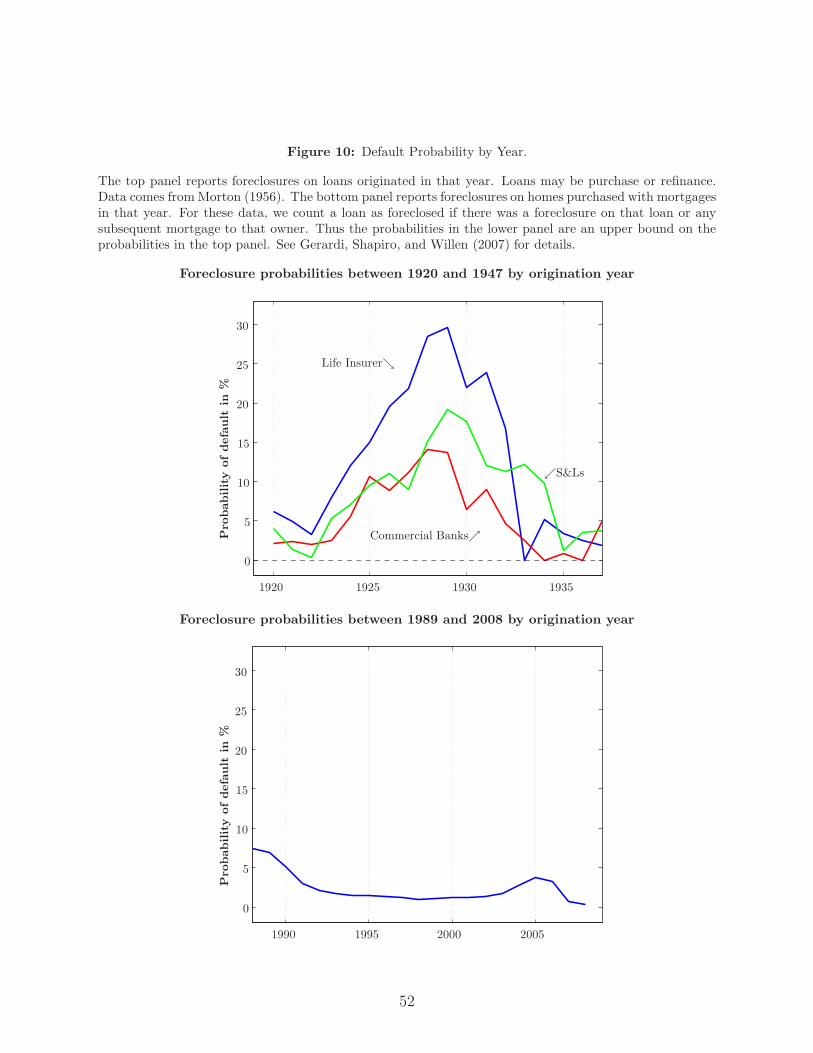
Figure 10: Default Probability by Year.

The top panel reports foreclosures on loans originated in that year. Loans may be purchase or refinance.Data comes from Morton (1956). The bottom panel reports foreclosures on homes purchased with mortgagesin that year. For these data, we count a loan as foreclosed if there was a foreclosure on that loan or anysubsequent mortgage to that owner. Thus the probabilities in the lower panel are an upper bound on theprobabilities in the top panel. See Gerardi, Shapiro, and Willen (2007) for details.

Foreclosure probabilities between 1920 and 1947 by origination year

0

5

10

15

20

25

30

1920 1925 1930 1935

Pro

bability

ofdefa

ult

in%

Life Insurerց

Commercial Banksր

ւS&Ls

Foreclosure probabilities between 1989 and 2008 by origination year

0

5

10

15

20

25

30

1990 1995 2000 2005

Pro

bability

ofdefa

ult

in%

52