NBER WORKING PAPER SERIES

THE VALUE OF SCHOOL FACILITIES:EVIDENCE FROM A DYNAMIC REGRESSION DISCONTINUITY DESIGN

Stephanie Riegg CelliniFernando Ferreira

Jesse Rothstein

Working Paper 14516http://www.nber.org/papers/w14516

NATIONAL BUREAU OF ECONOMIC RESEARCH1050 Massachusetts Avenue

Cambridge, MA 02138December 2008

We thank Janet Currie, Joseph Gyourko, David Lee, Chris Mayer, Cecilia Rouse, and Tony Yezer,as well as seminar participants at Brown, Chicago GSB, Duke, Harris School of Public Policy, IIES,University of Oslo, NHH, Penn, Princeton, Yale, NBER Labor Economics and NBER Public Economicsfor helpful comments and suggestions. Fernando Ferreira would like to thank the Research SponsorProgram of the Zell/Lurie Real Estate Center at Wharton for financial support. Jesse Rothstein thanksthe Princeton University Industrial Relations Section and Center for Economic Policy Studies. Wealso thank Igar Fuki, Scott Mildrum, Francisco Perez Arce, and Michela Tincani for excellent researchassistance. The views expressed herein are those of the author(s) and do not necessarily reflect theviews of the National Bureau of Economic Research.

NBER working papers are circulated for discussion and comment purposes. They have not been peer-reviewed or been subject to the review by the NBER Board of Directors that accompanies officialNBER publications.

© 2008 by Stephanie Riegg Cellini, Fernando Ferreira, and Jesse Rothstein. All rights reserved. Shortsections of text, not to exceed two paragraphs, may be quoted without explicit permission providedthat full credit, including © notice, is given to the source.

The Value of School Facilities: Evidence from a Dynamic Regression Discontinuity DesignStephanie Riegg Cellini, Fernando Ferreira, and Jesse RothsteinNBER Working Paper No. 14516December 2008JEL No. C23,H21,H41,H71,H75,I22,R13

ABSTRACT

This paper analyzes the impact of voter-approved school bond issues on school district balance sheets,local housing prices, and student achievement. We draw on the unique characteristics of California'ssystem of school finance to obtain clean identification of bonds' causal effects, comparing districtsin which school bond referenda passed or failed by narrow margins. We extend the traditional regressiondiscontinuity (RD) design to account for the dynamic nature of bond referenda, since the probabilityof future proposals depends on the outcomes of past elections. By law, bond revenues can be usedonly for school facilities projects. We find that bond funds indeed stick exclusively in the capital account,with no effect on current expenditures or other revenues. Our housing market estimates indicate thatCalifornia school districts under-invest in school facilities: passing a referendum causes immediate,sizable increases in home prices, implying a willingness-to-pay on the part of marginal homebuyersof $1.50 or more for each $1 of facility spending. These effects do not appear to be driven by changesin the income or racial composition of homeowners, and the school bond impact on test scores cannotexplain more than a small portion of the total housing price effect. Our estimates indicate that parentsvalue improvements in other dimensions of school output (e.g., safety) that may be not captured bytest scores.

Stephanie Riegg CelliniGeorge Washington UniversityTrachtenberg School of Public Policy and Public Administration805 21st Street, NW, MPA 601MWashington, DC 20052scellini@gwu.edu

Fernando FerreiraThe Wharton SchoolUniversity of Pennsylvania1461 Steinberg - Dietrich Hall3620 Locust WalkPhiladelphia, PA 19104-6302and NBERfferreir@wharton.upenn.edu

Jesse RothsteinIndustrial Relations SectionFirestone LibraryPrinceton UniversityPrinceton, NJ 08544and NBERjrothst@princeton.edu

I. Introduction

Federal, state, and local governments spend more than $50 billion per year to build and

renovate public schools (U.S. Department of Education 2007). Despite this, many of the more

than 97,000 public elementary and secondary schools in the United States are in need of

renovation, expansion, and repair. Fully a third of public schools rely on portable or temporary

classrooms and a quarter report that environmental factors, such as air conditioning and lighting,

are “moderate” or “major” obstacles to instruction (U.S. Department of Education 2007, Table

98). Notwithstanding, little is known about the importance of facility quality to educational

production.

Two central difficulties plague the literature on the effects of school resources, both

applicable to the effects of capital spending as well.1 First, resources may be endogenous to

schooling outcomes. The few studies that have focused explicitly on the effects of capital

expenditures on student achievement are unable to convincingly separate the causal effects of

school facilities from other confounding factors, such as the socioeconomic status of local

families. Second, many of the effects of resources may be reflected only imperfectly in student

achievement, so even a credible causal estimate of the effect on test scores might miss many of

the benefits. This seems likely to be a particular problem for school facilities, for which the

benefits may be concentrated in nonacademic outcomes like student health and safety.

This latter challenge is often avoided by focusing on the impacts of school spending on

housing markets. If homebuyers value school spending at the margin more than they value the

taxes they will pay to finance it, spending increases should lead to increases in housing prices.2

Indeed, in standard Tiebout (1956)-style models, a positive effect of tax increases on property

values is direct evidence that the initial tax rate is inefficiently low. As in studies of the impact

of resources on achievement, however, causal identification of this effect is quite challenging.

1 Hanushek (1996) reviews more than 90 studies and 400 estimates of the impact of school resources on achievement and concludes that “[s]imple resource policies hold little hope for improving student outcomes”. Card and Krueger (1996) dispute Hanushek’s interpretation of the literature. See also Hanushek (1986, 1997); Card and Krueger (1992); and Heckman, Layne-Farrar and Todd (1996). On facilities specifically, see Jones and Zimmer (2001); Schneider (2002); and Uline and Tschannen-Moran (2008). 2 See Oates (1969); Dee (2000); Palmon and Smith (1998); Starrett (1981); Barrow and Rouse (2004); and Bradbury, Mayer and Case (2001). A related body of research uses housing markets to measure household willingness to pay for school quality. See Rosen (1974) for an economic interpretation of the hedonic model, and Black (1999); Bayer, Ferreira, and McMillan (2007); Kane, Riegg, and Staiger (2006); and Rothstein (2006) for empirical applications.

1

In this paper, we implement a new research design to estimate the causal effects of school

facility spending. Our design takes advantage of the unique characteristics of California’s school

finance system to isolate exogenous variation in spending. While most school finance in

California is extremely centralized and offers little local discretion, California school districts

can issue general obligation bonds to finance the construction, improvement, and maintenance of

school facilities.3 Proposed bond measures must be approved in local referenda, and districts

that approve bond issues are likely to differ on both observable and unobservable dimensions

from those that do not. Districts in which bonds pass or fail by very narrow margins, however,

are likely to be quite similar on average.4 Taking advantage of the underlying continuity in

district characteristics around the threshold for bond approval, we use a regression discontinuity

(RD) framework to identify the causal impact of bond funding on district outcomes.

Several previous papers have used elections as sources of identification in RD models.5

Our analysis is complicated, however, by the dynamic nature of the bond proposal process. A

district that narrowly rejects an initial proposal is likely to consider and pass a new proposal

shortly thereafter, while a district that passes a bond measure this year is unlikely to pass another

measure next year. Moreover, bond effects are not immediate and may occur at different lags for

the different types of outcomes that we examine. We develop two estimators, both new to the

literature, that extend the RD design to identify the dynamic treatment effects of bond passage in

the presence of repeated elections with variable lags. We apply these estimators to a rich data set

combining two decades of information on bond referenda with annual measures of school district

spending, housing prices, district-level demographics, and student test scores.

Our first results concern the allocation of bond-funded revenues. Although these

revenues are earmarked for local capital improvements, theory predicts that districts will find

ways to divert resources toward non-capital purposes.6 We find strong evidence against this

prediction. Bond revenues stick entirely in the local capital account and we reject even small

effects on either current spending or other revenue sources. Estimates of the impact of a bond

passage can thus be interpreted as the effects of investments in school facilities.

3 Voter approved bonds are also common in other states, including Massachusetts, Ohio, Pennsylvania and Florida. 4 Early discussions of the RD design include Thistlethwaite and Campbell (1960) and Cook and Campbell (1979). For recent overviews, see Hahn, Todd, and Van der Klaauw (2001) and Imbens and Lemieux (2007). 5 See, e.g., Lee (2001, 2008), Lee, Moretti, and Butler (2004), DiNardo and Lee (2004), Cellini (forthcoming), Pettersson-Lidbom (2008), and Ferreira and Gyourko (2009). 6 See, e.g., Bradford and Oates (1971a, 1971b) and Knight (2002).

2

We next turn to an analysis of housing prices. We find that passage of a bond measure

causes housing prices in the district to rise by about six percent. This effect persists for at least a

decade. The implied elasticity of home prices with respect to school spending is approximately

0.5. This is slightly higher than, but consistent with, elasticities obtained by previous studies of

unrestricted spending (e.g., Barrow and Rouse, 2004; Bradbury, Mayer, and Case, 2001).

We find little evidence of changes in the income or racial composition of local

homebuyers following the passage of a bond, but there is some evidence of an effect on student

achievement six years after the bond issue. The point estimates indicate an increase of 0.07

student-level standard deviations in both math and reading scores, about one third as large as the

effect of reducing class sizes from 22 to 15 students in the Tennessee STAR experiment

(Krueger, 1999, 2003). However, this effect is imprecise – we cannot reject that all lagged

effects of bond passage on achievement are zero – and not entirely robust. Moreover, even an

effect of this size can explain only a small portion of the increase in housing prices. Evidently,

much of the value of school facilities to homeowners derives from dimensions of school output

that are not reflected in student test scores. This highlights the importance of using housing

markets—rather than simply test score gains—to evaluate school investments.

Our results provide clear evidence that school districts under-invest in school facilities, as

homebuyers value a dollar of school facility spending at much more than $1. The implied

willingness-to-pay via higher purchase prices and expected future property taxes is never smaller

than $1.13, and our preferred estimates are $1.50 or more. While much of the public choice

literature emphasizes the potential for over-spending by “Leviathan” governments, our results

suggest that the opposite is the case. Caution is required, however, in attempting to generalize

these results beyond our sample. California districts face unusual barriers to additional spending,

particularly in the capital account, and marginal returns may be lower in other states. Even

within our sample effects may differ for districts that are not at the margin of approving a bond

issue. Nevertheless, finding that marginal investments in school facilities have positive impacts

on housing prices and (perhaps) student achievement is an important result: California-style

restrictions on local public good provision evidently have important efficiency costs.

The remainder of the paper is organized as follows: Section II describes the California

school finance system. Section III develops simple economic models of resource allocation and

capitalization. Section IV describes our research design and introduces our estimators of

3

dynamic treatment effects. Section V describes the data, Section VI validates our regression

discontinuity strategy, and Section VII presents our estimates. Section VIII concludes.

II. California School Finance

California was historically known for its high quality, high spending school system. By

the 1980s and 1990s, however, California schools were widely considered underfunded. In

1995, per-pupil current spending was 13 percent below the national average, ranking the state

35th in the country despite its relatively high costs. Capital spending was particularly stingy, 30

percent below the national average.7 California schools became notorious for their

overcrowding, poor physical conditions, and heavy reliance on temporary, modular classrooms

(see, e.g., New York Times 1989).

Much of the decline in school funding has been attributed to the state’s shift to a

centralized system of finance under the 1971 Serrano v. Priest decision and to the passage in

1978 of Proposition 13, which eliminated school districts’ flexibility to set tax and spending

levels and, moreover, starved the state of revenue with which to assist districts.8 In 1984,

however, voters approved Proposition 46, which allowed school districts to issue general

obligation bonds to finance capital projects and to raise the local property tax rate for the

duration of the bonds in order to pay them off.9 Bonds must be approved by referendum.

Initially, a 2/3 vote was required, but beginning in 2001 proposals that adhered to certain

restrictions could qualify for a reduced threshold of 55%. Brunner and Reuben (2001) attribute

32% of California school facility spending between 1992-93 and 1998-99 to local bond

referenda. The leading alternative source of funds was state aid.10

The ballot summary for a representative proposal reads:

Shall Alhambra Unified School District repair, upgrade and equip all local schools, improve student safety conditions, upgrade electrical wiring for technology, install fire safety, energy efficient heating/cooling systems, emergency lighting, fire doors, replace outdated plumbing/sewer systems, repair leaky

7 Statistics in this paragraph are computed from U.S. Department of Education (2007), Table 174, and U.S. Department of Education (1998), Tables 165 and 42. 8 See Fischel (1989), Shapiro and Sonstelie (1982) and Sonstelie, Brunner, and Ardun (2000) for further details and discussion of California’s school finance reforms. 9 Local electorates can also approve parcel taxes for school funding, though these are comparatively rare. Parcel tax revenues have fewer restrictions than bonds (Orrick, Herrington & Sutcliffe, LLP, 2004). Although we focus on general obligation bonds in the analysis below, we present some specifications that incorporate parcel taxes as well. 10 The state aid formula depends on building age and capacity. If bond revenues are used to expand capacity or replace old school buildings, passage may reduce the district’s eligibility for state aid. We investigate this below.

4

rundown roofs/bathrooms, decaying walls, drainage systems, repair, construct, acquire, equip classrooms, libraries, science labs, sites and facilities, by issuing $85,000,000 of bonds at legal rates, requiring annual audits, citizen oversight, and no money for administrators' salaries? (Institute for Social Research 2006)

Bond revenues must go to pre-specified capital projects. Anecdotally, bonds are

frequently used to build new permanent classrooms that replace temporary buildings (e.g.,

Sebastian 2006). But repair and maintenance are also permissible uses, raising the possibility

that districts that were previously funding maintenance out of unrestricted funds might divert

those funds to other purposes when bonds are approved.

629 of the 1,035 school districts in California voted on at least one bond measure

between 1987 and 2006. The average number of measures considered (conditional on any) was

slightly more than two.11 Many of the elections were close: 35% were decided by less than five

percent of the vote. Table 1 shows the number of measures proposed and passed in each year,

along with the average bond amount (in 2000$ per pupil), the distribution of required vote shares

for bond approval, and the mean and standard deviation of observed vote shares.

Balsdon, Brunner, and Rueben (2003) study the decision to propose and pass a bond

measure. We add one point to their discussion: California’s unique property tax rules affect

voters’ incentives regarding bond measures. Under Proposition 13, assessed values are frozen at

the most recent sale price. This means that older families face disincentives to move after

children leave the home (Ferreira 2007), which may reduce willingness to support the public

schools. There is also substantial variation within districts in the tax price of local spending, as

new buyers pay a share of any tax increases that is far out of proportion to their share of the

district’s total property values. We discuss implications of these incentives below.

III. Theoretical Framework

A. School Resources, Flypaper Effects, and Student Achievement

Studies of school resources often invoke an “educational production function” that links

school resources—facilities, teacher quality, and class size, for example—to measurable student

outcomes. If school districts allocate resources optimally to their most productive uses,

exogenous increases in unrestricted school funding should improve student outcomes. Evidence

11 These data come from the California Education Data Partnership. More details are provided in Section V. 264 districts had only one measure on the ballot between 1987 and 2006, while 189 districts had 2, 99 districts had 3, 53 districts had 4, and 30 districts had 5 or more measures. The maximum was 10 measures.

5

that resources do not affect outcomes has often been taken as an indication that schools are

inefficiently managed (e.g., Hanushek 1986, 1997).

In theory, it should not matter whether marginal resources are restricted to certain

purposes, such as capital expenditures: districts will simply divert unrestricted funds away from

those targeted categories, with no effect on the total allocation. The only exception would arise

if the districts are at a corner solution, devoting none of their unrestricted funds to the targeted

categories. We present a simple model illustrating this in Appendix A.

Despite this well-known, widely accepted theory, a large body of evidence documents an

empirical anomaly: restricted grants tend to stick, even when the pre-grant allocation to the

targeted account is non-zero. This so-called “flypaper” effect is well documented in a variety of

settings, most notably in the context of intergovernmental grants (e.g. Bradford and Oates 1971a,

1971b).12 Knight (2002), however, has challenged the evidence for flypaper effects, arguing that

most papers do not adequately account for the endogeneity of intergovernmental grants.

Our regression discontinuity design represents a solution to this endogeneity problem, as

it permits us to identify the causal effect of restricted funding on both resource allocations and

other revenues (e.g. state aid). In our empirical analysis we further distinguish between districts

where prior spending patterns indicate that the restriction should or should not be binding. We

find strong evidence of flypaper effects for both sets of districts, and are able to reject even small

spillovers and crowd-out effects.

These results imply that our analysis of earmarked bonds will identify the impact of a

specific type of school resource—school facilities. It is an open question whether capital

improvements will lead to improved student achievement. Education researchers and reformers

often cite overcrowded classrooms; poor ventilation, indoor air quality, temperature control, or

lighting; inadequate computer hardware or wiring; and broken windows or plumbing as problems

that can interfere with student learning. Mitigating these types of environmental conditions may

bring substantial gains to student achievement in the short-run by reducing distractions and

missed school days (see Earthman 2002, Mendell and Heath 2004, and Schneider 2002 for

reviews). Improved conditions may also benefit teachers—reducing absenteeism, improving

12 Gordon (2004) finds that flypaper effects of intergovernmental grants are short-lived, but Barrow and Rouse (2004) find persistent effects. Flypaper effects have also been documented in corporate finance (Kaplan and Zingales 1997) and, more recently, in intra-household consumption (Duflo and Udry 2004), and individual investment decisions (Choi, Laibson, and Madrian 2007). See Hines and Thaler (1995) for a survey.

6

morale, and potentially reducing turnover (Buckley, Schneider, and Shang, 2005)—all of which

may in turn impact student achievement (e.g. Clotfelter, Vigdor, and Ladd 2007). But direct

evidence regarding the effects of investments in school facilities is in extremely short supply.

Importantly, the services provided by capital investments may be reflected only

imperfectly in student test scores. Infrastructure improvements may produce improvements in

student safety, athletic and art training, or the aesthetic appeal of the campus, all of which may

be valued by parents or homeowners, without any effect on academic achievement.

B. Voting, Housing Prices and the Value of School Facilities

One way to sidestep the challenges inherent in the measurement of school outputs is to

focus on the revealed preferences of parents and homeowners, as seen in housing markets. Local

net-of-tax housing prices should reflect the utility that home-buyers derive from the full menu of

local public goods. In this study, we examine compensated funding shifts, additional revenues

that are accompanied by an increased tax burden. Thus, if funds are misspent or simply yield

smaller benefits than would the consumption that must be foregone due to increased taxes, pre-

tax housing prices should fall when bond proposals pass. By contrast, if the effect on school

output is valued more than the foregone non-school consumption, home prices will rise when

bonds are passed. It can be shown that the efficient choice of spending levels will equate the

marginal utility of consumption with that of school spending (Samuelson, 1954), so positive

price effects imply that the prior spending level was inefficiently low.

The development of a full equilibrium model of house prices, household location

decisions and provision of local public goods is beyond the scope of this paper.13 We merely

provide a bit of intuition regarding the factors that determine home price effects due to

exogenous school investments. Among other simplifications, we neglect heterogeneity in

residents’ tax shares and housing consumption. We assume that the utility of family i living in

district j depends on local school output Aj, exogenous amenities Xj, and other consumption ci: uij

= Ui(Aj, Xj, ci). The consumer has income wi and faces the budget constraint ci ≤ wi – rj – pj,

where rj represents taxes and pj is the (rental) price of local housing. Service quality depends on

tax revenues, Aj = A(rj); if districts use funds inefficiently, A’(r) will be low.

13 The basic model is due to Brueckner (1979, 1982, 1983). Barrow and Rouse (2004) provide an accessible discussion. For more complex models that incorporate sorting and voting, see Epple, Filimon and Romer (1984, 1993), Benabou (1993) and Nechyba (1997).

7

We first discuss the household location decision, taking spending as given, and then

discuss the preferences of voters. A family chooses the community that provides the highest

utility, taking into account housing prices, taxes, and service quality. Writing the family’s

indirect utility in district j as U(A(rj), Xj, wi – rj – pj), the implicit function theorem yields the

family’s bid for housing in district j as a function of amenities and taxes, gij = gi(Xj, rj).14 This

bid-rent function depends on the prices, amenities, and tax rates of all other communities in the

family’s choice set; taking these as given, community j will provide higher utility than any

alternative community so long as pj < gij.

The family’s willingness-to-pay (WTP) for a marginal increase in rj in its chosen district

is ∂gi(Xj, rj)/∂rj. It can be shown that

(1) ∂gi(Xj, rj)/∂rj = (∂U/∂c)-1[A’(rj) * (∂U/∂A)] - 1.

This WTP is positive if the marginal product of school revenues multiplied by the

marginal utility of school outputs (in brackets) exceeds the marginal utility of consumption.

Ignoring momentarily the effect of spending on local housing prices, the family’s optimal tax

and service level satisfies ∂gi(Xj, rj)/∂rj = 0. If ∂gi(Xj, rj)/∂rj > 0, the district’s spending is below

the family’s preferred level; if ∂gi(Xj, rj)/∂rj < 0, the family would prefer that taxes and services

be cut.

In equilibrium, the price of housing in district j, p*(Xj, rj), equals the bid of the marginal

consumer, who must be indifferent between this district and another alternative. Thus, pj will

respond positively to increases in rj if and only if the prior level of school spending was below

the preferred level of the marginal resident.

When a tax increase takes place, low-WTP residents will tend to leave the community

and be replaced by in-movers with higher WTP. If higher-income families have higher

willingness-to-pay for school quality, tax increases may lead to increases in the mean income of

district residents. Because A may depend directly on community composition, A’(r) will reflect

both the direct effect of spending on achievement and an indirect effect operating through effects

of r on the characteristics of the district’s students. House prices will reflect both, plus an

additional component if families directly value high income neighbors (Bayer, Ferreira and

McMillan, 2004). In the empirical analyses below we investigate the effects of bond passage on

the racial composition and average income of new homebuyers and enrolled students.

14 gi() is defined implicitly by U(A(rj), Xj, wi – rj – gi(Xj, rj)) = maxk≠j U(A(rk), Xk, wi – rk – pk).

8

Tax changes are not exogenous, but depend on election outcomes. Many models of

voting focus on absentee landlords, who should vote for any proposal that would lead to an

increase in housing rents. To the extent that spending levels are set by such landlords, taxes will

be set at the property-value-maximizing level. The first-order effect of an exogenous change in

tax rates will be zero. But absentee landlords do not vote; residents do. There are several

circumstances in which residents will oppose spending increases even though ∂p*(Xj, rj)/∂rj > 0.

Most obviously, any renter who values spending less than the marginal resident – for whom

∂gi(Xj, rj)/∂rj < ∂p*(Xj, rj)/∂rj – will vote against a proposed spending increase, as the utility she

will derive from higher spending will not compensate her for the increased rent that she will pay.

Similarly, a homeowner who does not wish to move will vote on the basis of her own bid-rent,

not the community’s price function, and will oppose a tax increase if ∂gi(Xj, rj)/∂rj < 0. Thus, in

general we should expect that even price-increasing proposals will attract some opposition.

There are several aspects of California’s tax and school finance system that will tend to

lead to under-provision relative to the preferences of marginal residents. First, property

valuations are frozen at the initial sale price. Where in other states “empty nesters” whose kids

have grown will tend to move to a smaller house in a low-service community, in California they

face strong incentives to remain in their original homes. Immobile empty nesters will likely

oppose tax increases, as they derive little utility from school spending and see only paper gains

from increases in home values. Second, California’s school finance is extremely centralized,

with little control over spending. Hoxby (2001) argues that California-type systems will tend to

lead to under-provision, at least in wealthy communities. If so, houses in high-spending districts

are under-supplied, and exogenous increases in r will lead to higher prices.

A final issue concerns timing. Capital projects take time to plan, initiate, and carry out,

so bonds issued today will take several years to translate into improved capital services. Thus,

direct measures of school outputs will reflect the effects of bond passage only with long lags.

House prices reflect the present discounted value of all future services less all future taxes, so

should rise or fall as soon as the outcome of the election is known.15 This may happen well

before the election if the outcome is easy to predict, but when the election is close there is likely

important information revealed on Election Day. Price effects may therefore be immediate.

15 By design, bonds decouple the timing of tax revenue from spending. This can create complex post-election price dynamics. We discuss these in an Appendix. The basic point that the net value of the bond-financed spending relative to the taxes needed to pay for it is capitalized on or before the date of the election is unchanged.

9

However, if house prices are sticky or homebuyers have imperfect information, it may take a few

years for prices to fully reflect the impact of bond passage. We are thus interested in measuring

the full sequence of dynamic treatment effects on each of our outcomes.

IV. Empirical Research Design

There are three components to our research design. First, we describe how our regression

discontinuity strategy approximates a randomized experiment, allowing us to estimate the

reduced-form effect of measure passage (relative to failure) on later outcomes free of bias from

the correlation between bond passage and unobserved district characteristics. Second, we extend

the simple regression discontinuity design to panel data. The panel structure allows us to control

for fixed sources of heterogeneity across districts, allowing a more precise estimate of the impact

of bond passage on later outcomes. Information on the outcomes of interest before the election

also permits a test of the RD assumptions. Third, we incorporate bond dynamics into the

analysis. As we show in Section VI, districts that reject a bond proposal in a close vote are quite

likely to approve a later proposal. This complicates the interpretation of the reduced-form

estimates. We describe two estimators for the dynamic treatment effects of bond passage that

rely to differing degrees on the RD strategy.

A. Regression Discontinuity

In general, school districts with higher test scores and graduation rates also have higher

property values, lower tax prices of school spending, and residents with greater willingness to

pay for school quality. The resulting correlation between school quality and locally funded

spending cannot be interpreted causally.

Close bond referenda provide a source of variation that can be used to overcome the

endogeneity of school spending. So long as there is some unpredictable component of the vote,

the outcome of a narrowly-decided election is approximately random and is therefore unlikely to

be correlated with other district characteristics (Lee, 2001, 2008).

Formally, let yj be the outcome of interest, and let bj be an indicator for whether the

measure was passed. Define νj as the vote share and ν* as the threshold required for passage,

then bj ≡ 1(νj ≥ ν*). Assuming a simple linear model, we can write

(2) yj = α + bjβ + μj,

10

where β is the causal effect of bond passage and μj characterizes all other determinants of the

outcome. In general, μj is likely to be correlated with bj. Note, however, that

(3) E[yj | νj] = α + E[bj | νj]β + E[μj | νj] = α + bjβ + E[μj | νj].

The key identifying assumption of the regression discontinuity design is that E[μj | νj] is

continuous at ν*. That is, while districts that pass and reject bond measures by large margins

may differ, districts that narrowly pass and narrowly reject bond measures are similar. With this

assumption, β is identified from the discontinuity of E[yj | νj] at ν*:

(4) * *

lim [ | ] lim [ | ]j j

j j j jv v v vE y E yν ν β

↓ ↑− = .

We consider two implementations of the RD design. First, we estimate the two terms on

the left side of (4) as means among elections with votes close to the threshold on either side:

(5) β̂ = E*[yj | ν* ≤ νj < ν* + ε] - E*[yj | ν* - ε < νj < ν*],

where E*[] is the sample mean. Second, using the full sample, we estimate

(6) yj = α + bjβ + P(νj, γ) + uj,

where P(νj, γ) is a polynomial in νj with coefficients γ. From (2), the error term in (6) is

(7) uj = μj - P(νj, γ) = (μj - E[μj | νj]) + (E[μj | νj] - P(νj, γ)),

Because bj is a deterministic function of νj, it is uncorrelated with μj - E[μj | νj]. Equation

(6) thus provides a consistent estimate of β if (E[μj | νj] - P(νj, γ)) is asymptotically uncorrelated

with bj. This will be true if E[μj | νj] is continuous everywhere and if the order of the polynomial

P(νj, γ) rises with the sample size.

We use the difference in means estimator (5) for graphical presentations. For tabular

results, we rely primarily on the polynomial estimator (6). We model P() as a cubic, though we

also explore more flexible forms. An important advantage of the polynomial estimator is that it

uses all of the data, even while asymptotically identifying β only from observations with νj close

to ν*. This is helpful when considering the dynamics of bond proposal and passage, as a district

that has multiple elections may see a close vote in one election but not in the others.

B. Regression Discontinuity with Panel Data

With panel data, let νjt denote the vote share for an election held in district j in year t, and

yj,t+τ denote the outcome in that district in year t+τ. Let βτ be the total effect of bond passage in t

11

on yj,t+τ (we discuss the interpretation of βτ momentarily). Adapting equation (6), a polynomial

RD estimator for βτ is:

(8) yj,t+τ = ατ + bjtβτ + P(νjt, γτ) + uj,t+τ .

Note that all of the coefficients are permitted to vary freely with τ. We use equation (8)

primarily to test the validity of the RD design. The causal effects of passing a measure in year t

on outcomes in t-1 and on the change from t-2 to t-1 are zero, but violations of the RD

assumption might lead to non-zero effects. We thus present estimates of β-1 and of β-1 - β-2 from

(8) to assess the validity of the research design. An indication that either is nonzero would imply

that measure passage is not as good as random conditional on P(νjt, γτ) (Rothstein, 2008).

Several of the outcomes that we consider (e.g., house prices) vary substantially across

districts. This suggests that the error term in (8) is likely to have an important district-specific

component, ujt+τ = λj + υjt+τ. The RD design ensures that λj is uncorrelated with bjt conditional

on the vote share polynomial, but this district error component nevertheless introduces

substantial residual variation. To permit more precise estimates, we adapt (8) to allow for a

component of outcomes that is common to the district in the years before and after an election.

For each (j, t) with an election, we stack observations from district j in years t-2 through t+6 and

estimate the following regression:16

(9) yj,t+τ = bjtβτ + P(νjt, γτ) + λjt + δt+τ + ατ + νjt*φτ + υjt+τ.

Here, λjt is a fixed effect for each measure. δ t+τ and ατ are absolute and relative year

fixed effects, respectively. νjt* ∈ {0.55, 0.667} measures the vote share required for passage of

the measure under consideration. βτ, γτ, and φτ are constrained to zero for τ ≤ 0.17

C. Dynamic Treatment Effects

We refer to (9) as our “reduced-form” estimator. It estimates the effect of bond passage

in year t on outcomes in t + τ without controlling for the passage of any intervening bonds in t +

1, t + 2, etc. Indicators for these bonds, {bj,t+1, bj,t+2, …}, can be seen as omitted variables in (9).

16 Note that observations may appear more than once in the sample, linked to different measures. For example, if a district had elections in 2000 and 2002, its 2001 outcomes would appear both for the first election (with τ = 1) and for the second (with τ = -1). We cluster by school district to account for the dependence that this creates. 17 For house price regressions we impose the constraints only for τ < 0, since passage may have immediate effects on prices. Here, the measure fixed effects are identified from τ = -1 and -2. When we exclude the measure effects and remove the constraints on β, γ, and φ, we obtain small and insignificant estimates of βτ for τ < 0.

12

The standard omitted variables bias formula can be used to relate the reduced form bond effects

from (9) to the true causal effects of bond passage, θτ:18

(10) βτ = θτ + πsθs

s=1

τ−1

∑ for τ > 1.

Here, πs is the reduced form effect of bond passage in year t on passage in year t+s, controlling

for a polynomial in νjt.19 We show in Section VI that πs is negative for 1 ≤ s ≤ 4, so we expect

the reduced form estimator to understate the true causal effects at lags of one or more years.

We use two estimators for the dynamic treatment effects. We refer to the first as the

“recursive” estimator. It is based directly on equation (10), which can be inverted to yield

recursive formulae for the dynamic treatment effects in terms of the reduced-form coefficients

and of the earlier direct effects: θ1 = β1, θ2 = β2 + π1θ1, and, in general,

(11) θτ = βτ − πsθs

s=1

τ−1

∑ for τ>1.

The recursive estimator thus proceeds in two steps. First, we use (9) to estimate the

reduced-form coefficients β and π, this time including all possible τ values in the sample.20

Second, we apply (11) recursively to compute the dynamic effects implied by the reduced-form

point estimates. Standard errors for θτ are obtained by the delta method.

One drawback of the recursive estimator is that θτ depends on all of the reduced-form

coefficients {βs, πs; 1 ≤ s ≤ τ}. As a result, the estimated effects become imprecise at long lags.

Our second approach, which we refer to as the “one-step” estimator, requires a stronger

assumption but yields more precise estimates. We use the full panel of observations on districts

18 Even θτ is in a sense a reduced-form effect, as we make no effort to control for second or third order intervening events – e.g., superintendent and mayoral elections – that may be influenced by bond passage. We also focus on the simple effect of bond passage, rather than the effects of the particular uses to which the bond revenues are put (e.g. window repairs, lighting improvements, new construction, etc.). 19 When θτ is constant across τ, equation (10) reduces to ( )1

11 ss

τ

τβ θ−

== + ∑ π , where

1

1 ss

τπ

−

=∑ represents the

reduced-form effect of passage in t on the probability of passing a subsequent measure. This is often referred to as a “fuzzy” RD design (Hahn, Todd, and Van der Klaauw 2001). Our recursive estimator can thus be seen as an extension of the usual IV estimator for fuzzy RDs that allows for dynamics in the treatment effect. See also Lee, Moretti and Butler (2004) for a related application. 20 In practice, we estimate a single regression stacking the two outcomes (yj,t+τ and bj,t+τ), fully interacting (9) with an indicator for the outcome type and clustering on the school district. This is equivalent to estimating the two reduced-form equations separately, but yields an estimate of the full sampling variance matrix for { 1β , …, τβ , 1π ,

…, τπ } allowing for covariance between the two.

13

over time, including each observation exactly once. We form an indicator, mjs, for whether

district j had a measure on the ballot in year s, and we set bjs = νjs = 0 whenever mjs = 0. We then

regress outcomes on a full set of lags of m, b, and P(ν), allowing all coefficients to vary with τ:

(12) ( )( ), , ,0

P ,jt j t j t j t j t jty m b uδ + . τ

τ τ τ τ τ ττ

α θ ν γ λ− − −=

= + + + +∑

As in the reduced-form estimator, we include time effects (δt) to absorb changes in the

price level. The district fixed effects (λj) absorb persistent differences across districts that are

unrelated to bond passage.21 Under the standard RD assumption that measure passage is as good

as randomly assigned conditional on a smooth function of νjt-s, any influence of past elections on

bj,t-s itself should be absorbed through the P(νj,t-s, γs) polynomial.

Relative to the reduced form equation (9), the one step estimator can be seen as

controlling for intermediate outcomes: passage of a bond in year t-τ may influence mj,t-s and νj,t-s

for any s < τ. Thus, the one-step estimator yields consistent estimates of the dynamic treatment

effects θτ only if these intermediate outcomes are uncorrelated with the error term in (12), ujt ,

conditional on νj,t-τ. In other words, we require that the comparison of treatment and control

groups around the threshold mitigates not only the bias due to endogenous school district

features but also the omitted variable bias due to other potential bond proposals. This additional

assumption is not required for the recursive estimator, which is based only on reduced form RD

estimates. In the empirical estimates below, we show that both estimators yield similar estimates

of the structural parameters βτ (suggesting that the additional one-step assumption is reasonable)

but that the one-step estimator is more precise.

Both the recursive and one-step approaches assume that bonds have no effect before they

are passed. But housing prices should in theory capitalize the discounted expected effects of

possible future bonds. When we allow for this, (10) becomes

(13) ( )1

( )0

0 1

1 ss s s

s s

rτ

ττ τ τ

τ

β θ π θ θ π− ∞

− −−

= = +

= + + +∑ ∑ ,

where r is the interest rate and θ0 is the immediate direct effect of a bond issue on house prices.

The final term in (13) reflects the forward-looking aspect of prices. Our main recursive

estimates use (11), but we also report estimates based on this augmented expression.

21 As in the static specification, we have also estimated versions of (13) that omit the district fixed effects and estimate the ατ, θτ, and γτ coefficients even for τ < 0.

14

V. Data

We obtain bond data from a database maintained by the California Education Data

Partnership. For each proposed bond, the data include the amount, intended purpose, vote share,

required vote share for passage, and voter turnout. Our sample includes all general obligation

bond measures sponsored by school districts between 1987 and 2006. We merge these to

district-level enrollment, revenue, and spending data from the Common Core of Data (CCD).

The data contain annual measures of capital and current expenditures, revenues, and long-term

debt between 1995 and 2006. We also extract from the CCD the number of schools, enrollment,

and student demographics, each measured annually.22

We obtain annual average home prices (averaged over all transactions) and the square

footage and lot size of transacted homes at the census block group level from a proprietary

database compiled from public records by the real estate services firm Dataquick. The

underlying data describe all housing transactions in California from 1988 to 2005.23 We used

GIS mapping software to assign census block groups to school districts.24

Our prices reflect only houses that sell during the year. If the mix of houses that transact

changes—for example, one might expect sales of houses that can accommodate families with

children to react differently to school spending than do smaller houses—this will lead our

measures to be biased relative to the quantity of interest, the prices of all houses in the district.

We take two steps to minimize this bias. First, when we average block groups to the district

level, we weight them by their year-2000 populations rather than by the number of

transactions.25 This holds constant the location of transactions within the district. Second, we

include in our models of housing prices controls for the average square footage and lot size of

transacted homes and for the number of sales to absorb any rem

aining selection.

We form a district-level panel of student achievement by merging results from several

different tests. From 2003 to 2007, the most consistently available measures are third grade

22 Some districts merge or split in two during our sample period. Where possible, we combine observations to form a consistent unit over time, adding the spending and enrollment data for the constituent districts. 23 The majority of housing transactions happen from May through August. We assign measures to housing data treating the year containing the first summer after the measure election as the year of the election. Thus, elections in November 2005 and April 2006 are both treated as occurring in 2006. This means that some of the housing transactions assigned to year 0 in fact occurred before the election. To merge measures to academic year data from the CCD, we treat any measure between May 2005 and April 2006 as occurring during the 2005-06 academic year. 24 When school district boundaries and block group boundaries do not line up we use population weights based on the proportion of a block group located within a school district. 25 Our results are robust to other schemes for weighting blocks within districts.

15

reading and math scores on the California Achievement Tests (CAT). The most comparable

measures in earlier years are based on the Stanford-9 exam, given each year between 1998 and

2002. Though developed by different publishers and therefore not directly comparable, both the

CAT and Stanford-9 exams are nationally-normed multiple-choice exams. We also use

California Learning Assessment System (CLAS) reading and math test scores for fourth graders

in 1993 and 1994. To account for differences in exams across years, we standardize the scaled

scores each year using school-level means and standard deviations.

Finally, we construct the racial composition and average family income of homebuyers in

each district between 1992 and 2006 from data collected under the Home Mortgage Disclosure

Act (HMDA). We use a GIS matching procedure similar to the one implemented for house

prices to map the tract-level HMDA data to school districts. We treat our measure as

characterizing in-migrants to the district, though we are unable to exclude intra-district movers

from the calculation. Note also that renters are not represented in these data.

Table 2 presents descriptive statistics. Column 1 shows the means and standard

deviations computed over all district-year observations in our data. Columns 2 and 3 divide the

sample between districts that proposed at least one measure between 1987 and 2006 and those

that did not. Districts that proposed measures are larger and have higher test scores, incomes,

and housing prices but smaller lot sizes.

Columns 4 and 5 focus on districts that approved and rejected school bonds, using data

from the year just before the bond election, while column 6 presents differences between them.

Districts that passed measures had 25% higher enrollment, $489 more in debt per pupil, $206

higher current instructional spending, and $349 higher total spending. Districts that passed

measures also had much higher incomes and house prices, but smaller lots.

VI. Testing the Validity of the Regression Discontinuity Design

A. Balance of Treatment and Control Groups

In light of the large pre-existing differences between districts that pass and fail measures,

it is important to verify that our regression discontinuity design can eliminate these differences.

We examine three diagnostics for the validity of the RD quasi-experiment, based on the

distribution of vote shares, pre-election differences in mean characteristics, and differences in

pre-election trends. Tests of the balance of outcome variable means and trends before the

16

election are possible only because of the panel structure of our data, and provide particularly

convincing evidence regarding the approximate randomness of measure passage.

Figure 1 shows the histogram of bond measure vote shares, separately for measures that

required 2/3 and 55% of the vote. Discontinuous changes in density around the threshold can be

an indication of endogenous sorting around this threshold, which would violate the RD

assumptions (McCrary, 2008). We see no evidence of such changes.

Columns 1-4 of Table 3 present regressions of fiscal, housing, and academic variables

measured in the year before a bond referendum on the election outcome, using the specification

described in equation (6). The first column controls only for year effects and the required

threshold. Like Table 2, it reveals large pre-measure differences in several outcomes. The

second column adds a cubic polynomial in the measure vote share. This addition eliminates

most of the significant estimates, shrinking the point estimates substantially.

The specifications in Columns 1-2 are estimated from a sample that includes only

observations from the year before the election. Columns 3-4 turn to panels pooling observations

from two years before through six years after the election. We generalize equation (9) by freeing

up the coefficients corresponding to outcomes in the year of and year before the election, and

report in the table the “effect” of bond passage in the year before the election, β-1. Column 3

reports estimates from a specification without measure fixed effects (λjt in (9)), while Column 4

includes them. Pooling the data does not substantially change the estimates. The specification in

Column 4, however, has much smaller (in absolute value) point estimates and standard errors,

particularly for housing prices and test scores. The fixed effects evidently absorb a great deal of

variation in these outcomes that is unrelated to election outcomes.

Columns 5-7 in Table 3 repeat our three first specifications, taking as the dependent

variable the change in each outcome between year t-1 and t. Although the model without

controls shows some differences in trends between districts that pass and fail measures, these are

eliminated when we include controls for the vote share. Overall, there seems to be little cause

for concern about the approximate randomness of the measure passage indicator in our RD

framework. Once we control for a cubic in the measure vote share, measure passage does not

appear to be correlated with pre-treatment trends of any of the outcomes we examine. Further, in

similar specifications (not reported in Table 3), we find no evidence of “effects” on sales

volume, housing characteristics, the income of homebuyers, or other covariates.

17

B. School Bond Dynamics

As noted earlier, school districts where a measure fails are more likely to propose and

pass a subsequent measure than are districts where the initial measure passes. This pattern is

particularly pronounced when the initial vote is close. Figure 2 shows the number of additional

measures considered (left panel) and approved (right panel) over the four years following an

election. We plot average counts across all measures in two-percentage-point bins defined by

the vote share relative to the threshold. Thus, the leftmost point in each panel represents

measures that failed by between 8 and 10 percentage points, the next measures that failed by 6 to

8 points, and so on. There is a clear discontinuity at measure passage. When the initial measure

passed, only about 10% of districts considered another measure shortly thereafter. By contrast,

the typical district where a measure failed narrowly considered approximately one additional

measure and passed 0.6 within four years.

Figure 3 offers another view, plotting reduced-form estimates (from specification (9)) of

the impact of measure passage on the probability of passing another measure τ years later. There

are negative effects in each of the first four years, summing to about -0.6 (as seen in Figure 2),

but there is no sign of any effect thereafter.

VII. Results

A. School District Spending and Flypaper Effects

We begin our investigation of the effects of measure passage by examining fiscal

outcomes. Figures 4, 5, and 6 present graphical analyses of long term debt, capital outlays and

current spending by margin of victory or defeat, respectively. As in Figure 2, we show average

outcomes (controlling for calendar year effects) in two-percentage-point bins defined by the vote

share relative to the threshold. These are computed separately for the year before the election

and for the third year after the election.26

There is no sign of a discontinuity in debt or capital spending in the year before the

election. By contrast, three years later, districts where the measure just passed have about

$3,000 more debt per pupil than districts where the measure narrowly failed, and spend about

26 The bin corresponding to measures that failed by less than 2 percentage points is the category excluded from the regression used to control for year effects, so estimates may be interpreted as differences relative to that bin. Results are robust to exclusion of the year controls.

18

$1,000 more per pupil on capital outlays. There is no evidence whatsoever of a similar

discontinuity in current spending, before or after the election.

Panel A of Table 4 presents reduced-form RD estimates of the effect of bond passage on

long term debt, capital outlays, current instructional expenditures, and state and federal transfers

(all in per-pupil terms) over the following six years, using specification (9). Bond passage has an

immediate impact on the stock of debt but no significant effect on the other fiscal outcomes in

the first year. It causes large increases in long term debt and capital expenditures in years 2, 3,

and 4, but these increases fade away by year 5. There is no indication of any effect on current

spending in any year, and confidence intervals rule out effects amounting to more than about

$100 per pupil in every year. This is dramatic evidence for flypaper effects—bond revenues

appear to “stick” entirely in the capital account. The estimates for state and federal transfers

demonstrate another form of flypaper effect: there is no indication that bond revenues crowd out

intergovernmental transfers, and indeed most of the point estimates are positive.

Recall from Section IV.C that reduced-form estimates are likely to be attenuated relative

to the true causal effect of passing a bond because they do not control for the presence of later

bonds. Panel B of Table 4 presents estimates of the dynamic treatment effects of bond passage,

first from our recursive estimator and then from the one-step specification. The effects on both

debt and capital spending are larger and more persistent than in Panel A, but again there is no

indication that current spending or intergovernmental transfers change after bond passage.

Appendix Table 1 presents estimates for a variety of additional balance sheet measures; again,

there is no sign of any spillover of bond passage towards other non-capital outlay items.

Figure 7 presents estimates of the dynamic treatment effects on capital spending all the

way out to the 15th year after the election. Neither estimator indicates that effects persist after

year 6. The one-step estimator has somewhat larger effects in every year than does the recursive

estimator, but the differences are small. Note that the confidence intervals for the one-step

estimator are much smaller than those for the recursive estimator, particularly at long lags.

Figure 8 shows similar dynamic treatment effects estimates of current instructional spending.

These are tightly estimated zeros in every year.

B. Housing Prices

Figure 9 provides a graphical analysis of the impact of bond passage on log housing

prices corresponding to the analyses of fiscal outcomes in Figures 4-6. Two important patterns

19

emerge. First, housing prices are positively correlated with vote shares, indicating that higher

priced districts are more likely to pass bond measures with larger margins of victory. Second, in

districts where bond measures were approved, housing prices appear to shift upward by 6 or 7

percentage points by the third year after the election relative to the pre-election prices. Such a

shift is not visible in districts where bonds failed.

Table 5 presents estimates of the reduced-form and dynamic treatment effects on log

housing prices. We augment each specification with controls for the average characteristics of

transacted homes. Because each regression also includes district or measure fixed effects, the

coefficients on these variables are identified from within-district, over-time changes in the value

of housing transactions. Their inclusion should ameliorate the bias coming from changes in the

types of homes transacted. We also allow for effects in the year of the election, since (in contrast

to fiscal outcomes) we expect homebuyers to respond immediately to the outcome.

Column 1 presents reduced-form estimates. House prices increase by 2.1% in the year of

bond passage, though this is not significantly different from zero. The estimated effects rise

slightly thereafter, reaching 5.8% and becoming significant three years after the election. Point

estimates fade somewhat thereafter and cease to be significant.

Columns 2 and 3 show estimates of dynamic treatment effects. As expected, these are

somewhat larger, and are uniformly significant after year 0. The estimates indicate that bond

approval in year t causes prices to rise by 2.8-3.0% in year t, 3.6-4.1% in year t+1 (holding t+1

bond issues constant), and 6.7-10.1% in t+6. Figure 10 plots the coefficients and confidence

intervals from the two dynamic specifications, showing estimates out to year 15. The recursive

estimator shows growing effects through almost the entire period, while the one-step estimator

yields a flatter profile. Confidence intervals are wide, particularly for the recursive estimator in

later periods, and a zero effect is typically at or near the lower bound of these intervals.27

However, as noted earlier, these estimated dynamic effects rely on a specification of the

time pattern of effects that does not allow for forward-looking housing prices. When we modify

the recursive estimator to allow prices to reflect rational expectations about future bonds as in

equation (13), the immediate effect of bond passage rises and the profile is flatter in the first few

years: point estimates in years 0 through 5 are 6.1%, 6.8%, 7.4%, 9.5%, 8.8% and 9.5%

27 The flexibility of these specifications reduces precision. When we constrain the one-step treatment effect to be constant over time, it is 4.9% (standard error 1.7%).

20

respectively. These are shown as hollow circles in Figure 10. Since it is not clear which of the

two recursive models more accurately reflects the true expectations of marginal homebuyers, we

expect that the true effect lies between the two sets of estimates.

C. Willingness to Pay for School Facility Investments

As discussed in Section III, a substantial effect of bond passage on prices indicates that

the marginal resident’s willingness-to-pay (WTP) for school services exceeds the cost of

providing those services and therefore school spending is inefficiently low. It is thus instructive

to compute the WTP implied by our estimated price effects. This calculation requires

assumptions about interest and discount rates, the speed with which new facilities are brought

into service, property tax shares, and the income tax deductibility of property taxes and mortgage

interest payments. We outline the calculations below, and describe the details in the Appendix.

The average house in districts with close elections (margins of victory or defeat less than

two percent) is worth $236,433, so a 3.0% effect on house prices raises the value of the average

house by approximately $7,100. Assuming a discount rate of 7.33%, 2.4 housing units per pupil,

and equal tax shares, the present discounted value of the increment to property taxes needed to

finance a $6,300 per pupil bond – the average in close elections – is about $1,950. Therefore,

new homeowners would have to pay a total additional cost in housing prices and property tax

increases of approximately $9,050 in order to get school spending benefits of $6,300 per pupil.

This corresponds to a WTP of about $1.44 for $1 per pupil in bond authorization.28 Alternative

calculations yield somewhat different WTPs, though all are well above $1. Our smallest

estimate, obtained when allowing for unequal property tax shares and income tax deductibility of

property tax and interest payments, is $1.13.

As Figure 10 suggests, the WTP is generally higher when we use our recursive estimates

of bond effects on house prices or when we measure the price effects several years after the

election. The 4th year price effect estimates, for example, range from $1.31 (one-step estimator

with full accounting for taxes) to $1.89 (recursive estimator without accounting for taxes and

using a discount rate of 5.24%). The sensitivity of WTP calculations to the year in which price

28 Our comparison of the cost per home to the bond amount per pupil is appropriate if the marginal homebuyer has one school-aged child. This almost exactly matches the average number of children in owner-occupied California households in the 2000 census who moved in 1999. While we do not compute standard errors for the WTP, note that WTP of $1 corresponds to zero effect on house prices, which we reject.

21

effects are measured may indicate that capitalization is not immediate.29 However, the forward-

looking price estimates indicate a WTP that is largely invariant to the year in which the price

effect is measured and around $2

Previous estimates of capitalization focus on price responses to permanent increases in

annual spending. When we convert the one-time expenditures financed by bonds to an

equivalent annual flow using discount rates of 5.24% and 7.33% (Barrow and Rouse, 2004), we

estimate an elasticity of prices with respect to school spending of 0.43 or 0.61, respectively. By

comparison, Bradbury, Mayer and Case (2001) and Hilber and Mayer (2004) find an elasticity of

0.23 in Massachusetts, though this rises to 0.57 when they focus on districts where state spending

caps are most binding. As California’s spending formula is unusually restrictive, the latter is

probably a better comparison. Barrow and Rouse (2004) focus on the impact of state aid

unaccompanied by tax increases. Their main results, from a national sample, imply elasticities

with respect to compensated spending less than one third the size of ours. Again, however, their

results are substantially larger when they focus on districts similar to California (in this case,

high income and education). Moreover, this comparison is extremely sensitive. If homebuyers

assume that changes in state aid formulas will be reversed after ten or twenty years, for example,

Barrow and Rouse’s implied price response is much closer to ours.

There are, however, important differences between our study and the earlier work. The

Bradbury-Mayer-Case, Hilber-Mayer, and Barrow-Rouse studies all examine unrestricted

spending. This should produce larger elasticities than does restricted spending. On the other

hand, the extremely low levels of capital investment in California may mean that the returns to

spending are considerably higher there than in other states.30 Finally, differences in estimates

may derive in part from differences in research designs; we are the first in this literature to

29 If capitalization is rapid and not affected by imperfect information or transaction costs, a simpler WTP calculation could be based on reduced-form estimates of the effects of bond passage on prices in year 0 – which should capitalize the present discounted value (PDV) of future taxes and benefits – and on the PDV of future spending. There are several drawbacks to this method, most notably that we observe a long panel of post-election spending for only the earliest referenda in our sample and that our “immediate” house price measure – average sales prices in the year of the election – may be contaminated by sales occurring before the election. If we ignore these issues, this simpler method implies a WTP of about $2.10. 30 Another potentially important difference is the structure of bond measures. Districts are required to announce the projects that will be undertaken before placing the measure on the ballot. This may impose some accountability for the use of the funds, limiting managers’ ability to divert the funds toward unproductive purposes. This would imply higher capitalization rates than for less carefully targeted funds.

22

employ a regression discontinuity framework. Overall, we interpret our capitalization estimates

as somewhat large but well within the range of plausible effect sizes implied by earlier work.

Since new homebuyers are willing to pay much more in house prices and property taxes

than the total new school investments per house, why do bond referenda ever fail? It is

important to stress that house price effects reflect the preferences of the marginal homebuyer. As

discussed in Section III, many voters make their decisions on the basis of their personal

valuations rather than the anticipated effect on home prices, and many residents may have lower

valuations than does the marginal homebuyer. Moreover, our estimates are local to districts

where measures barely pass, typically with a 2/3 vote. The returns to investment in these

districts may be higher than elsewhere, and in particular the many districts that have never

considered a bond measure may have much lower returns.

D. Robustness

Table 6 presents a variety of alternative specifications meant to probe the robustness of

our results. To conserve space we report only the estimates from our one-step specification of

the effect of bond approval on outcomes four years later. Column 1 reports the baseline

estimates. Columns 2-4 vary the vote share controls: Column 2 includes only a linear control;

Column 3 allows for three linear segments, with kinks at 55% and 67% vote shares; and Column

4 allows separate cubic vote share-outcome relationships in the [0, 55%], [55%, 67%], and [67%,

100%] ranges. None of these yields evidence contrary to our main results.

Columns 5-7 report estimated discontinuities at locations other than the threshold

required for passage; in each of these specifications, we also allow a discontinuity at the actual

threshold. In column 5, we estimate the discontinuity in our outcomes at the counterfactual

threshold, 55% when ν* = 2/3 and 2/3 when ν* = 55%, while columns 6 and 7 show estimates for

placebo thresholds 10 percentage points above or below the true threshold. Only two of the

fifteen coefficients measuring discontinuities at counterfactual thresholds are statistically

significant, and there is no clear pattern to the coefficients.

Column 8 investigates whether our evidence for flypaper effects arises because districts

are at corner solutions with respect to capital spending. We estimate our reduced-form

specification for the subsample of districts with above-median ($562 per pupil) capital spending

per pupil in the year before the election. These districts should have had plenty of room to divert

23

pre-existing funds into the current account after passing bond measures. As in the full sample,

however, there is no sign of any effect on current spending even among these districts.

In addition to bonds, districts can impose parcel taxes that generate unrestricted revenues,

though these are relatively rare. Parcel taxes may be substitutes for bonds, potentially

confounding the effect of bond passage on house prices. To examine this, we generalize our

one-step specification, adding indicators for the presence of a parcel tax measure in each relative

year τ and for its passage.31 Column 9 reports the bond passage coefficient when parcel taxes

are controlled. The estimated bond effects are unchanged. The parcel tax coefficients (not

reported) are significantly indistinguishable both from zero and from the bond coefficients.

We have also estimated a specification that restricts the sample to elections before 2001.

This addresses several concerns about our main estimates. In particular, this sample excludes all

55% elections, so price effects are identified only from elections requiring a two-thirds

supermajority, and it allows us to use a constant sample for computation of various lags of the

treatment effects (at least up to τ = 6). Not surprisingly, the subsample estimates are less precise

than those from our main sample, but there are no systematic differences in the point estimates.

E. Academic Achievement

Passage of a bond measure appears to lead to large increases in a school district’s capital

spending, no change in current spending, and substantial house price appreciation. Taken

together, these results reveal that improvements in school facilities yield outputs that

homebuyers value. These outputs may include academic achievement.

Table 7 reports estimates of the effect of bond passage on third grade reading and math

scores. The effects are small and insignificant for the first several years. This result is expected

given the time it takes to execute capital projects; the flow of services should not begin for

several years. However, the point estimates are generally positive and seem to gradually trend

upward. This pattern is easier to see in Figure 11, which plots the point estimates and confidence

intervals from the math score specifications. By year six, we see large, significant effects in the

reduced-form and one-step specifications, corresponding to about one-sixth of a school-level

standard deviation. Point estimates fall back to zero thereafter, however.32

31 We constrain the vote share polynomial to be the same for the two types of measures. 32 The sample size drops significantly after year 6—only 58% of districts remain in our sample in year 7.

24

It is not clear that much can be learned from these estimates: we cannot reject zero effects

in every year, but the confidence intervals also include large positive effects. In terms of the

more familiar student-level standard deviations, the year-six point estimates correspond to effects

of roughly 0.067 for reading and 0.077 for math.33 If taken literally, these imply that bond-

financed improvements to existing facilities raise achievement by about one third as much as a

reduction in class sizes from 22 to 15 students (Krueger 1999, 2003).34

Even this maximal interpretation of the test score results, however, cannot account for the

full house price effects seen earlier. Previous research on school quality capitalization (see

Bayer, Ferreira and McMillan (2007), Black (1999), and Kane, Riegg, and Staiger (2006)) has

found that a one school-level standard deviation increase in test scores raises housing prices

between four and six percent. This implies that our estimated year-six effect on test scores

would produce a housing price increase just over one percent.35

The majority of our estimated effects on housing prices must therefore be attributable to

non-academic school outputs. These may be particularly important in the case of school

facilities improvements. Parents may value new playgrounds or athletic facilities for the

recreational opportunities they provide; enhanced safety from a remodeled entrance or drop-off

area; and improved child health from asbestos abatement and the replacement of drafty

temporary classrooms, even if these do not contribute to academic achievement. New facilities

may also be physically appealing, perhaps enhancing the desirability of the neighborhood. Any

improvements in these unobservable dimensions of school output will lead to housing price

effects that exceed those reflected in student achievement measures. The potential relevance of

these channels underscores the importance of using housing markets—rather than simply test

scores gains—to value school investments.

F. Household Sorting

Recent empirical studies of the capitalization of school quality emphasize the importance

of social multiplier effects deriving from preferences for wealthy neighbors (see, e.g., Bayer,

Ferreira and McMillan, 2004). If wealthy families have higher willingness-to-pay for school

33 We use the ratio of school-level to student-level standard deviations on the 2007 California Standards Tests (CST) to convert school-level to student-level SDs. 34 We find no evidence that bond passage affects teacher-pupil ratios, or that the results could be attributable to the construction of new, smaller schools. Results are available upon request. 35 An increase of .185 of a school-level standard deviation in test scores multiplied by an effect of 6 percentage points would yield a price increase of just 1.1 percentage point.

25

output, passage of a bond may lead to increases in the income of in-migrants to the district,

creating follow-on increases in the desirability of the district, in house prices, and in test scores.

In Panel A of Table 8 we report dynamic RD estimates for the impact of bond approval

on sales volumes. Volumes would be expected to rise if passage leads to changes in the sort of

families that prefer the school district. The estimates show that sales volumes increase by 200-

300 units per year. An analysis of log volumes indicates about a 3% increase in sales, though

this is not statistically significant.36

The remainder of Table 8 examines effects on population composition directly. In Panel

B, we report effects on the characteristics of new homebuyers. We find no distinguishable effect

on average income or on racial composition (as measured by the share white and Asian). Panel

C reports effects on the student population. We find no impact on enrollment, racial

composition, or average parental education across all grades.37

Since we have only limited data on population changes, it could be that sorting effects are

concentrated in dimensions that we do not measure (e.g., tastes for education or the presence of

children). Even so, sorting is not likely to account for our full price effect. The literature

indicates that social multiplier effects on house prices could be as large as 75% of the direct

effect of school quality (Bayer, Ferreira and McMillan, 2004). This would imply that at most 2.5

percentage points of the estimated 6% price effect in year three could be due to sorting, still

leaving a large portion that must be attributable to increased school output.

VIII. Conclusion

In this paper we use a “dynamic” regression discontinuity design to estimate the value of

school facilities to parents and homeowners. Drawing on the unique characteristics of

California’s system of school finance, we identify the effects of capital investments on housing

prices by comparing districts in which school bond referenda passed or failed by narrow

margins. Unlike districts where bond referenda garnered overwhelming voter support or

36 Sales volume could also represent an increase in the local supply of homes. We are unable to disentangle supply and demand effects because yearly data on housing supply is not available. However, we test whether bond passage leads to a change in the composition of houses by estimating our dynamic RD model for housing features such as square footage and lot size. No composition effects are observed. 37 We have also looked at effects on enrollment in early grades, where composition effects may appear first. We find no change in Kindergarten or 1st grade enrollment. We do find a small, permanent increase in the fraction of white and Asian students in Kindergarten, though not in first grade even several years later. One potential explanation is that some families switched from private to public Kindergartens after bond passage; some bond proposals specify building additional classrooms to permit conversion from half-day to full-day Kindergarten.

26

opposition, the set of districts with close votes are likely to be similar to each other in both

observable and unobservable characteristics. The analysis is complicated, however, by the

tendency for districts in which proposed bonds are rejected to propose and pass additional

measures in future years. Our dynamic RD estimators account for these feedback effects,

bringing the identification power of a traditional RD design into a panel data context.

We first examine the impact of passing a bond on school spending. We find sharp and

sizable flypaper effects. Bond approval increases capital outlays, and there is no sign that any

funds are diverted toward current spending. This is surprising: the inclusion of repairs and

maintenance on the list of allowed bond-funded projects would seem to provide ample room for

districts to divert previously unrestricted funds, but this appears not to happen. One possible

explanation is that the requirement to announce capital projects in advance makes it difficult to

divert funds toward non-capital uses.

The strong flypaper effect implies that our subsequent analyses can be interpreted as

revealing the effects of school facilities. We find that passing a measure causes home prices to

rise by six percent or more. As theory predicts, most of this effect appears well in advance of the

completion of the funded projects. We also find some evidence of effects on student

achievement several years after bond passage, but no sign of effects on the income or racial

composition of the school district. The home price effects presumably reflect the anticipation of

increased school output, though it seems likely that much of the effect derives from dimensions

of output (such as safety) that are not picked up by test scores.

Our results provide clear evidence that California districts at the margin of passing a bond

are spending well below the economically efficient level, with returns to additional spending far

in excess of the cost. Evidently, the referendum process erects too large a barrier to the issuance

of bonds and prevents many worthwhile projects. A loosening of California’s constraints on

local spending would apparently yield substantial economic benefits. Our results may have

similar implications for other states and localities with low levels of capital investment and

highly centralized systems of school finance.

27

References

Balsdon, Ed, Eric J. Brunner, and Kim Rueben (2003), "Private Demands for Public Capital: Evidence from School Bond Referenda," Journal of Urban Economics 54(3), p. 610-638.

Barrow, Lisa, and Cecilia Rouse (2004), “Using Market Valuation to Assess Public School Spending,” Journal of Public Economics 88, p. 1747-1769.

Bayer, Patrick, Fernando Ferreira, and Robert McMillan (2004), “Tiebout Sorting, Social Multipliers, and the Demand for School Quality,” NBER Working Paper #10871.

Bayer, Patrick, Fernando Ferreira, and Robert McMillan (2007), “A Unified Framework for Measuring Preferences for Schools and Neighborhoods,” The Journal of Political Economy 115(4), p. 588-638.

Benabou, Roland (1993), “The Workings of a City: Location, Education, and Production,” Quarterly Journal of Economics 108(3), p. 619-652.

Black, Sandra E. (1999), “Do Better School Matter? Parental Valuation of Elementary Education,” Quarterly Journal of Economics 114(2), p. 577-599.

Bradbury, Katharine, Christopher Mayer, and Karl Case (2001), “Property Tax Limits, Local Fiscal Behavior, and Property Values: Evidence from Massachusetts under Proposition 2 ½,” Journal of Public Economics 80, p. 287-311.

Bradford, David, and Wallace Oates (1971a), “The Analysis of Revenue Sharing in a New Approach to Collective Fiscal Decisions,” Quarterly Journal of Economics 85(3), p. 416-439.

Bradford, David, and Wallace Oates (1971b), “Towards a Predictive Theory of Intergovernmental Grants,” American Economic Review Papers and Proceedings 61(2), p. 440-448.

Brueckner, Jan K. (1979), "Property Values, Local Public Expenditure and Economic Efficiency," Journal of Public Economics 11(2), p. 223-245.

Brueckner, Jan K. (1982), "A Test for Allocative Efficiency in the Local Public Sector," Journal of Public Economics 19(3), p. 311-331.

Brueckner, Jan K. (1983), "Property Value Maximization and Public Sector Efficiency," Journal of Urban Economics 14(1), p. 1-15.

Brunner, Eric J., and Kim Rueben (2001), “Financing New School Construction and Modernization: Evidence from California,” National Tax Journal 54(3), p. 527-539.

Buckley, Jack, Mark Schneider, and Yi Shang (2005), “Fix It and They Might Stay: School Facility Quality and Teacher Retention in Washington, DC,” The Teachers College Record 107(5), p. 1107-1123.

Card, David, and Alan Krueger (1992), “Does School Quality Matter? Returns to Education and the Characteristics of Public Schools in the United States,” Journal of Political Economy 100(1), p. 1-40.

28

Card, David, and Alan Krueger (1996), “School Resources and Student Outcomes: An Overview of the Literature and New Evidence from North and South Carolina,” Journal of Economic Perspectives 10(4), p. 31-50.

Cellini, Stephanie Riegg (forthcoming), “Crowded Colleges and College Crowd-Out: The Impact of Public Subsidies on the Two-Year College Market,” American Economic Journal: Economic Policy.

Choi, James J., and David Laibson, and Brigitte C. Madrian (2007), "The Flypaper Effect in Individual Investor Asset Allocation," NBER Working Papers #13656.

Clotfelter, Charles, Helen Ladd, and Jacob Vigdor (2007), “Are Teacher Absences Worth Worrying About in the U.S.?” NBER Working Papers #13648.

Cook, Thomas, and Donald Campbell (1979), Quasi-experimentation: Design and Analysis Issues for Field Settings. Boston: Houghton Mifflin.

Dee, Thomas S. (2000), “The Capitalization of Education Finance Reforms,” The Journal of Law and Economics 43(1), p. 185-214.

DiNardo, John, and David S. Lee (2004), “Economic Impacts of New Unionization on Private Sector Employers: 1984-2001,” Quarterly Journal of Economics 119(4), p. 1383-1441.

Duflo, Esther and Christopher Udry (2004), "Intrahousehold Resource Allocation in Cote d'Ivoire: Social Norms, Separate Accounts and Consumption Choices," NBER Working Papers #10498.

Earthman, Glen I. (2002), School Facility Conditions and Academic Achievement. Los Angeles, CA: UCLA’s Institute for Democracy, Education, and Access (IDEA).

Epple, Dennis, Radu Filimon, and Thomas Romer (1984), "Equilibrium among Local Jurisdictions: Toward an Integrated Approach of Voting and Residential Choice," Journal of Public Economics 24, p. 281-308.

Epple, Dennis, Radu Filimon, and Thomas Romer (1993), “Existence of Voting and Housing Equilibrium in a System of Communities with Property Taxes,” Regional Science and Urban Economics 23, p. 585-610.

Ferreira, Fernando (2007), “You Can Take It with You: Proposition 13 Tax Benefits, Residential Mobility, and Willingness to Pay for Housing Amenities,” mimeo, The Wharton School, University of Pennsylvania.

Ferreira, Fernando, and Joseph Gyourko (2009), “Do Political Parties Matter? Evidence from U.S. Cities,” forthcoming, Quarterly Journal of Economics.

Fischel, William (1989), “Did Serrano Cause Proposition 13?” National Tax Journal 42(4), p. 465-73.

Gordon, Nora (2004), "Do federal grants boost school spending? Evidence from Title I," Journal of Public Economics 88(9-10), p. 1771-1792.

Hahn, Jinyong, Petra Todd, and Wilbert Van der Klaauw (2001), “Identification and Estimation of Treatment Effects with a Regression Discontinuity Design,” Econometrica 69(1), p. 201-209.

29

Hanushek, Eric A. (1986), “The Economics of Schooling: Production and Efficiency in Public Schools,” Journal of Economic Literature 24(3), p. 1141-1177.

Hanushek, Eric A. (1996), “School Resources and Student Performance” In Burtless, Gary, Ed., Does Money Matter? The Effect of School Resources on Student Achievement and Adult Success. Washington, D.C., Brookings Institution, p. 43-73.

Hanushek, Eric A. (1997), “Assessing the Effects of School Resources on Student Outcomes: An Update,” Educational Evaluation and Policy Analysis 19(2), p. 141-164.

Heckman, James, Anne Layne-Farrar, and Petra Todd (1996), “Human Capital Pricing Equations with and Application to Estimating the Effect of School Quality on Earnings,” Review of Economics and Statistics 78, p. 562-610.

Hilber, Christian, and Christopher Mayer (2004), “School Funding Equalization and Residential Location for the Young and the Elderly,” Brookings-Wharton Papers on Urban Affairs, p. 107-148.

Hines, James R., and Richard H. Thaler (1995), "The Flypaper Effect," Journal of Economic Perspectives 9(4), p. 217-26.

Hoxby, Caroline M. (2001), “All School Finance Equalizations are not Created Equal,” Quarterly Journal of Economics 116(4), p. 1189-1231.

Imbens, Guido, and Thomas Lemieux (2007), “Regression Discontinuity Designs: A Guide to Practice,” NBER Working Papers #13039.

Institute for Social Research (2006), California Elections Data Archive, http://www.csus.edu/isr.

Jones, John T., and Ron W. Zimmer (2001), “Examining the Impact of Capital on Academic Achievement,” Economics of Education Review 20, p. 577-588.

Kane, Thomas J., Stephanie K. Riegg, and Douglas O. Staiger (2006), “School Quality, Neighborhoods, and Housing Prices,” American Law and Economics Review 8(2), p. 183-212.

Kaplan, Steven N., and Luigi Zingales (1997), “Do Investment-Cash Flow Sensitivities Provide Useful Measures of Financing Constraints?” Quarterly Journal of Economics 112(1), p. 169–215.

Knight, Brian (2002), “Endogenous Federal Grants and Crowd-out of State Government Spending: Theory and Evidence from the Federal Highway Aid Program,” American Economic Review 92(1), p. 71-92.

Krueger, Alan. B. (1999), "Experimental Estimates of Education Production Functions," Quarterly Journal of Economics 114(2), p. 497-532.

Krueger, Alan. B. (2003), "Economic Considerations and Class Size," The Economic Journal 113, p. F34-F63.

Lee, David (2001), “The Electoral Advantage to Incumbency and Voters’ Valuation of Politicians’ Experience: A Regression Discontinuity Analysis of Elections to the U.S. House,” NBER Working Papers #8441.

Lee, David (2008), “Randomized Experiments from Non-random Selection in U.S. House Elections,” Journal of Econometrics 142(2), p. 675-697.

30

Lee, David S., Enrico Moretti, and Matthew J. Butler (2004), “Do Voters Affect or Elect Policies? Evidence from the U.S. House,” The Quarterly Journal of Economics (August), p. 807-859.

McCrary, Justin (2008), “Manipulation of the Running Variable in the Regression Discontinuity Design: A Density Test,” Journal of Econometrics 142(2), p. 698-714.

Mendell, Mark J. and Garvin A. Heath (2004), “Do Indoor Environments in Schools Influence Student Performance? A Critical Review of the Literature.” Indoor Air 15(1), p. 27-52.

Nechyba, Thomas J. (1997), “Existence of Equilibrium and Stratification in Local and Hierarchical Tiebout Economies with Property Taxes and Voting,” Economic Theory 10, p. 277-304.

New York Times (1989), “Births and Immigration Squeeze California Classroom Space,” New York Times, October, 8, 1989.

Oates, Wallace E. (1969), "The Effects of Property Taxes and Local Public Spending on Property Values: An Empirical Study of Tax Capitalization and the Tiebout Hypothesis," Journal of Political Economy 77(6), p. 957-71.

Orrick, Herrington & Sutcliffe, LLP. (2004), School Finance Bulletin. Public Finance Department of Orrick, Herrington, and Sutcliffe: San Francisco, CA. http://www.orrick.com/fileupload/259.pdf

Palmon, Oded, and Barton A. Smith (1998), “New Evidence on Property Tax Capitalization,” The Journal of Political Economy 106(5), p. 1099-1111.

Pettersson-Lidbom, Per (2008), “Do Parties Matter for Economic Outcomes: A Regression-Discontinuity Approach,” Journal of the European Economic Association, 6(5), p. 1037-1056.

Rosen, Sherwin (1974), "Hedonic Prices and Implicit Markets: Product Differentiation in Pure Competition," Journal of Political Economy 82(1), p. 34-55.

Rothstein, Jesse (2006), “Good Principals or Good Peers: Parental Valuation of School Characteristics, Tiebout Equilibrium, and the Incentive Effects of Competition among Jurisdictions,” American Economic Review 96(4), p. 1333-1350.

Rothstein, Jesse (2008), “Teacher Quality in Educational Production: Tracking, Decay, and Student Achievement,” NBER Working Papers #14442.

Samuelson, Paul A. (1954), “The Pure Theory of Public Expenditure,” The Review of Economics and Statistics 36(4), p. 387-389.

Schneider, Mark (2002), Do School Facilities Affect Academic Outcomes? National Clearinghouse for Educational Facilities. Washington, DC.

Sebastian, Simone (2006), "Schools Measure Proposed," San Francisco Chronicle, March 8, 2006, p. B-1.

Shapiro, Perry, and Jon Sonstelie (1982), “Did Proposition 13 Slay Leviathan?” American Economic Review 72(2), p. 184-90.

Sonstelie, Jon, Eric Brunner, and Kenneth Ardun (2000), For Better or For Worse? School Finance Reform in California, Public Policy Institute of California: San Francisco.

31

Starrett, David A. (1981), “Land Value Capitalization in Local Public Finance,” The Journal of Political Economy 89(2), p. 306-327.

Thistlethwaite, Donald L., and Donald T. Campbell (1960), “Regression-Discontinuity Analysis: An Alternative to the Ex-Post Facto Experiment,” Journal of Educational Psychology 51, p. 309-317.

Tiebout, Charles (1956), “A Pure Theory of Local Public Expenditures”, Journal of Political Economy 64(5), p. 416-424.

Uline, Cynthia and Megan Tschannen-Moran (in press), “The Walls Speak: The Interplay of Quality Facilities, School Climate, and Student Achievement,” The Journal of Educational Administration.

U.S. Department of Education, National Center for Education Statistics (NCES), (1998), Digest of Education Statistics 1998. http://nces.ed.gov/programs/digest/d98/index.asp.

U.S. Department of Education, National Center for Education Statistics (NCES), (2007), Digest of Education Statistics 2007. http://nces.ed.gov/programs/digest/d07/index.asp.

32

Appendix A: Resource Allocation with Restricted Funding Under fairly general conditions, an optimizing school district given additional restricted

revenues will divert some of the additional revenues to other purposes, by reducing the allocation of unrestricted revenues to the targeted accounts. This prediction will fail to hold only if the district was previously at a corner solution, allocating no revenue to the targeted accounts; in this case, there is no possibility of diversion.

A school district receives funding y from federal and state transfers plus local revenues; we treat all as exogenous to local decisions. The district allocates this funding across school facilities (k) and current inputs such as teachers and textbooks (e). Let A measure educational outputs, and suppose that the educational production function is A = f(k, e). If revenues are unrestricted, the district maximizes A subject to the budget constraint k+e ≤ y. Let k(y) and e(y) be the optimal resource choices; these will sum to total revenues, k(y) + e(y) = y, and (assuming an interior solution) will equate the marginal product of each type of spending, f1(k(y), e(y)) = f2(k(y), e(y)). For typical production functions, both k(y) and e(y) will be increasing in y. Thus, a grant of additional unrestricted revenues r will lead to increases in both capital and current spending, k(y+r)>k(y) and e(y+r)>e(y).

Now suppose that the new revenues are restricted to the capital account. One might expect this sort of restricted grant to increase capital revenues by the full amount r, to k(y) + r. But this is usually not so. The grant restrictions simply add an additional constraint, k ≥ r. This can be satisfied with much smaller increases if k(y) > 0. An optimizing district will re-allocate unrestricted revenues toward the current account. That is, rather than choosing (k(y) + r, e(y)), the district will devote only k* < k(y) of its unrestricted revenues to the capital account, leading to a total capital allocation of k*+r<k(y)+r and total current spending of e* > e(y).

The degree of diversion will depend on the extent to which the k ≥ r constraint is binding. In one extreme, it is not binding at all – the district would have chosen capital spending greater than r even without constraints (k(y+r) > r). In this case, the restriction has no effect on the district’s allocation decisions. For this sort of district, the passage of a restricted bond is predicted to lead to increases in both capital and current spending identical to those that would be seen with an unrestricted revenue grant.

On the other extreme, a district might, if unconstrained, choose to spend nothing on capital (k(y+r)=0). In this case, the restriction is extremely effective: The district cannot devote a negative amount of its unrestricted budget toward the capital account. It instead selects a corner solution, setting k* = 0 and e* = y. This yields total capital spending of r and total current spending of y. The additional revenues thus “stick” entirely in the capital account, with no spillovers to the current account.

Of course, there are intermediate cases. If k(y) > 0 but k(y+r) < r, a restricted grant will lead to more capital spending than would an unrestricted grant, but less than would occur if the district were unable to re-optimize upon receipt of the grant.

33

Appendix B: Willingness-to-Pay and Elasticity Calculations This appendix describes how the effects of bond passage on house prices can be converted to obtain estimates of the marginal homebuyer’s willingness-to-pay for school spending and of the elasticity of house prices with respect to school spending. We make a number of assumptions in the calculations. We assume that the interest rate on bonds is 4.6%, that a rental unit is equivalent to 0.6 owner-occupied units, and that the tax burden is divided evenly among all of the (owner-equivalent) housing units in the district. We consider a bond issue of $6,309 per pupil, with a 30-year maturity, in a district with average housing price of $236,433 and 2.4 owner-equivalent units per pupil.38 We consider two discount rates, 7.33% and 5.24%, both taken from Barrow and Rouse (2004). We begin with the willingness-to-pay for additional spending. We assume that marginal homebuyers have exactly one school-aged child per household and that the price effects reflect the willingness-to-pay for a per-pupil share of the average bond. The estimates in Column 3 of Table 5 indicate that bond passage raises prices by 3.02% in the first year, or $7,136 for the average house. Property taxes must rise by $163 per year per house in order to pay off the bond. The present discounted value of these taxes is $1,952 (ρ1 = 7.33%) or $2,431 (ρ2 = 5.24%). Thus, the total cost is $7,136 + $1,952 = $9,087 (ρ1) or $7,136 + $2,431 = $9,567 (ρ2). With 2.4 homes per pupil, a single home’s share of the average bond issue is $2,629. If we assume that marginal homebuyers have exactly one school-aged child per household, the implied WTP for $1 in spending on the household’s children is $1.44 (ρ1) or 1.52 (ρ2). Table 5 indicates that the price effects are larger a few years after the election than in the first year. By this point, some of the taxes will already have been paid, but (assuming that planning and executing a construction project takes several years) none of the benefits will have been received. Moreover, because the arrival of benefits is approaching, these benefits will be discounted to a lesser degree. Thus, a constant WTP would imply rising price effects over this period. The estimated WTP (based on our one-step estimates) is 1.63 in year 2, 2.12 in year 3, and 1.70 in year 4 (for ρ1; ρ2 implies 1.76, 2.31, and 1.89, respectively). It is not possible to extend these estimates beyond year 4, as the assumption that all of the benefits arrive after that date is untenable. Recursive estimates yield somewhat larger WTP, rising from 1.38 in year 0 to 2.35 in year 4 (with ρ1). The forward-looking estimates imply still larger WTP but much smaller increases over time, from $2.60 in year 0 to $2.74 in year 6 (with ρ = 7.33%). This suggests that the dynamic pattern of tax payments can account for nearly all of the slope seen in Figure 10. The calculations thus far omit two tax considerations. First, because California freezes valuations at the original purchase price, new homebuyers pay a disproportionate share of property taxes. Using Ferreira’s (2007) tabulation of effective property tax rates in California, we compute that property tax increment that raises $1 per house will cost a new homebuyer about $1.35 and a long-term resident only about $0.58. This implies that the above calculations understate the tax burden borne by new buyers. Offsetting this, however, is the income tax deductibility of property tax payments and mortgage interest payments. When we incorporate both of these features into the calculation, the estimated WTP falls by about 20%. Even with this adjustment, our one-step estimates imply that marginal homebuyers are willing to give up at least

38 The bond amount and housing price are the means among districts with measures that pass or fail by less than 2%. The equivalence of a rental unit with 0.6 owner-occupied units is computed by comparing the present discounted value of the California mean monthly rent for a renter-occupied unit in 2000 (using a 5.24% discount rate) with the mean value of owner occupied homes. The count of housing units per pupil is the average in our sample; the average for districts with close elections is similar.

34

$1.35 (ρ1) or $1.50 (ρ2) in consumption in order to provide $1 per pupil to the school district’s capital budget.39 The recursive estimates indicate larger WTP, around $2 in our forward-looking calculation and $1.80 otherwise.

Bradbury, Mayer, and Case (2001) and Hilber and Mayer (2004) report the elasticity of home prices with respect to annual school spending rather than the WTP. To estimate this, we first compute the size of the annuity that yields the same discounted value as the temporary spending increase made possible by the bonds. This is $462 (ρ1) or $330 (ρ2). Next, we divide this by annual per pupil spending (in the year of the election, averaged over all districts where a measure passed or failed by less than two percentage points), $6,767. The bond measures therefore represent an increase in the flow of spending of 6.8% (ρ1) or 4.9% (ρ2). Comparing these to the housing price effects from Table 5, Column 3, we obtain elasticities of year-0 prices with respect to spending of 0.44 or 0.61, respectively. Elasticities of year-4 prices are 0.68 and 1.03, again depending on the discount rate. Barrow and Rouse (2004) estimate the effect of state aid—which they interpret as free transfers—on aggregate home prices, both measured in per pupil terms. To adapt our results to a similar metric, we first convert our effects on house prices to effects on property values per pupil. The estimates from Table 7, Column 4 indicate price effects of $7,136 in year 0 and $12,348 in year 4. Multiplying this by 2.4 housing units per pupil, we find effects of $17,126 in year 0 and $29,635 in year 4. Comparing these to the average bond value, $6,309, we estimate that school spending with present discounted value of $1 per pupil raises aggregate property values by $2.71 in year 0 and $4.70 in year 4.

Barrow and Rouse’s (2004) estimates represent the effect of free transfers, while the bond spending studied here must be paid for by increased property taxes. To compute the effect of tax-financed spending implied by Barrow and Rouse’s estimates, we first note that they compare their results to the null hypothesis that prices rise by $1 per dollar of present discounted value of future state aid. The ratio of their estimates to the null, less one, can therefore be interpreted as the effect of $1 of state aid to be paid for with $1 in taxes (both in present value). Their main specification yields an estimated coefficient of 30.285; this corresponds to a housing price effect per dollar of bonds of 0.16 (with a discount rate of 5.24%) to 0.63 (with a discount rate of 7.3%).

While these estimates are lower than our findings, several further considerations help reconcile these results. First, Barrow and Rouse find much greater capitalization in better-educated and higher-income districts. To the extent that California’s education and income levels are higher than the national average, we would expect Barrow and Rouse’s estimate for all districts to underestimate the housing price effect for the state. Barrow and Rouse’s estimates for the top 80% of districts by education (as measured by the share of the population without a high school diploma) yield a range of 0.42 – 0.99, while their estimates for the top quintile of districts by average household income yield 2.52-3.93. Further, the interpretation of their results is quite sensitive to the discount rate: using a 10% discount rate, their estimates of the effect on property values range from 1.1 for all districts to 5.7 for the top quintile. Finally, Barrow and Rouse’s estimates reflect the value of a permanent increase in state aid, while homebuyers might be uncertain about the permanency of the policy changes they examine. If the stream of state aid is expected to persist for only 20 years, the implied effect on property values per dollar of future spending is much larger. Thus, our estimates are not out of line with theirs. 39 These WTP figures are based on the year-4 effects. We assume that new homebuyers will have tax shares 30% above average over the life of the bond, that they finance 80% of the increment to home prices using a 30-year mortgage with a fixed 8% interest rate, and that interest is fully deductible with a marginal income tax rate of 32%.

35

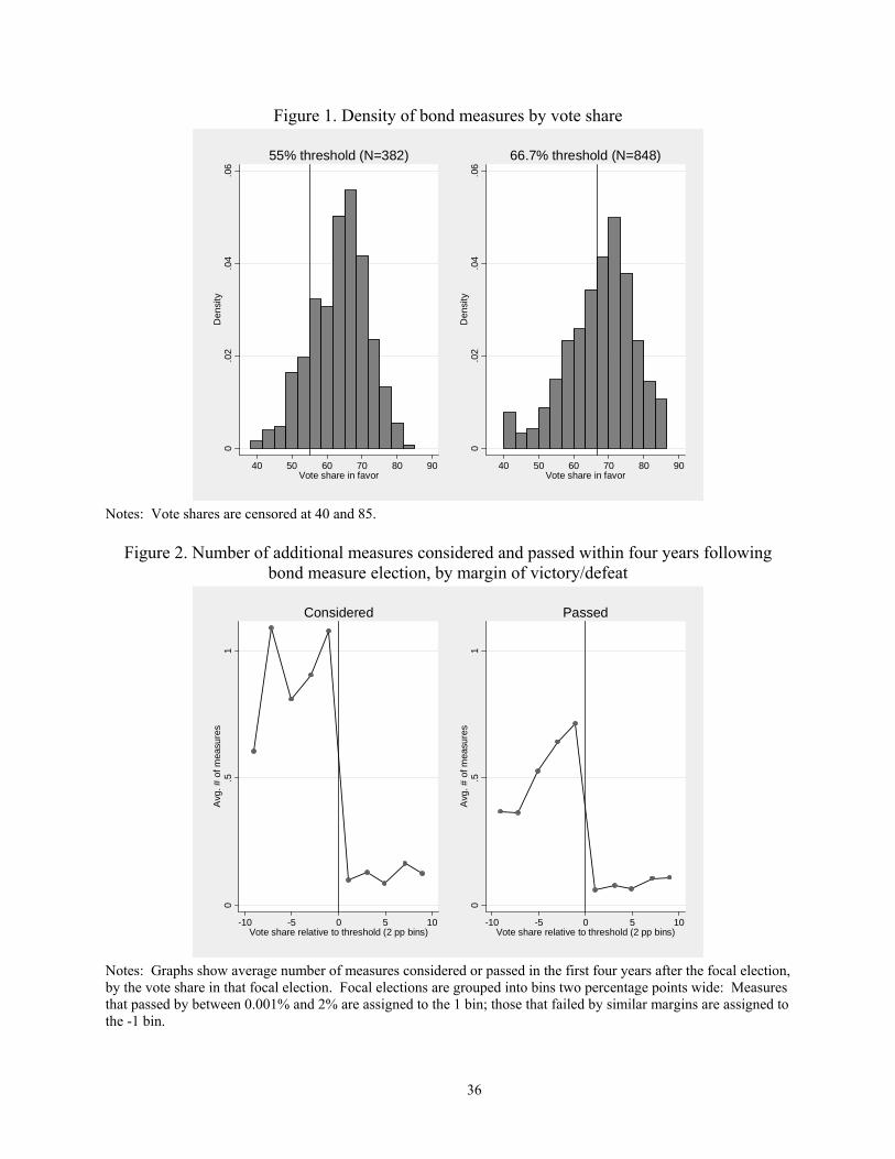
Figure 1. Density of bond measures by vote share

0.0

2.0

4.0

6D

ensi

ty

40 50 60 70 80 90Vote share in favor

55% threshold (N=382)

0.0

2.0

4.0

6D

ensi

ty40 50 60 70 80 90

Vote share in favor

66.7% threshold (N=848)

Notes: Vote shares are censored at 40 and 85.

Figure 2. Number of additional measures considered and passed within four years following bond measure election, by margin of victory/defeat

0.5

1A

vg. #

of m

easu

res

-10 -5 0 5 10Vote share relative to threshold (2 pp bins)

Considered

0.5

1A

vg. #

of m

easu

res

-10 -5 0 5 10Vote share relative to threshold (2 pp bins)

Passed

Notes: Graphs show average number of measures considered or passed in the first four years after the focal election, by the vote share in that focal election. Focal elections are grouped into bins two percentage points wide: Measures that passed by between 0.001% and 2% are assigned to the 1 bin; those that failed by similar margins are assigned to the -1 bin.

36

Figure 3. Reduced form RD estimates of the effect of bond passage on the probability of passing a later bond, by years since the focal election

-.50

.51

Effe

ct o

n pr

(pas

s bo

nd)

0 3 6 9 12 15Year (relative to election)

Reduced-form RD estimate95% CI

Notes: Graph shows coefficients and 95% confidence intervals for the effect of measure passage in year t on the probability of passing a measure in year t+τ. The specification is the reduced-form regression described in equation (9). Sample includes relative years -19 through +19, excluding 0 (when the effect is mechanically one). Figure 4. Long term debt per pupil, by vote share, one year before and three years after election

-100

00

1000

2000

3000

Mea

n lo

ng te

rm d

ebt P

P

-10 -5 0 5 10Vote share relative to threshold (2 pp bins)

Year before election Three years after election

Notes: Graph shows average long term debt per pupil in each bin. Averages are conditional on year fixed effects, and the -1 bin is normalized to zero. Measures that passed by between 0.001% and 2% are assigned to the 1 bin; those that failed by similar margins are assigned to the -1 bin.

37

Figure 5. Capital outlays per pupil, by vote share, one year before and three years after election

-500

050

010

00M

ean

capi

tal o

utla

ys P

P

-10 -5 0 5 10Vote share relative to threshold (2 pp bins)

Year before election Three years after election

Notes: Graph shows average capital outlays per pupil in each bin in the listed year relative to the election. Averages are conditional on year fixed effects, and the -1 bin is normalized to zero. Measures that passed by between 0.001% and 2% are assigned to the 1 bin; those that failed by similar margins are assigned to the -1 bin.

Figure 6. Current instructional expenditures per pupil, by vote share, one year before and three

years after election

-500

050

010

00M

ean

curr

ent i

nstr.

exp

endi

ture

s P

P

-10 -5 0 5 10Vote share relative to threshold (2 pp bins)

Year before election Three years after election

Notes: Graph shows average current instructional expenditures per pupil in each bin in the listed year relative to the election. Averages are conditional on year fixed effects, and the -1 bin is normalized to zero. Measures that passed by between 0.001% and 2% are assigned to the 1 bin; those that failed by similar margins are assigned to the -1 bin.

38

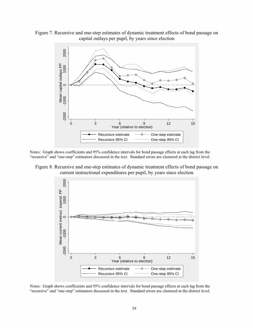
Figure 7. Recursive and one-step estimates of dynamic treatment effects of bond passage on capital outlays per pupil, by years since election

-200

0-1

000

010

0020

00M

ean

capi

tal o

utla

ys P

P

0 3 6 9 12 15Year (relative to election)

Recursive estimate One-step estimateRecursive 95% CI One-step 95% CI

Notes: Graph shows coefficients and 95% confidence intervals for bond passage effects at each lag from the “recursive” and “one-step” estimators discussed in the text. Standard errors are clustered at the district level.

Figure 8. Recursive and one-step estimates of dynamic treatment effects of bond passage on current instructional expenditures per pupil, by years since election

-200

0-1

000

010

0020

00M

ean

curr

ent i

nstru

ct. e

xpen

d. P

P

0 3 6 9 12 15Year (relative to election)

Recursive estimate One-step estimateRecursive 95% CI One-step 95% CI

Notes: Graph shows coefficients and 95% confidence intervals for bond passage effects at each lag from the “recursive” and “one-step” estimators discussed in the text. Standard errors are clustered at the district level.

39

Figure 9. Log housing prices by vote share, one year before and three years after election

-.10

.1.2

.3m

ean

log

hous

ing

pric

es

-10 -5 0 5 10Vote share relative to threshold (2 pp bins)

Year before election Three years after election

Notes: Graph shows average log housing prices in each bin in the listed year relative to the election. Averages are conditional on year fixed effects and the -1 bin was normalized to zero. Measures that passed by between 0.001% and 2% are assigned to the 1 bin; those that failed by similar margins are assigned to the -1 bin.

Figure 10. Recursive, one-step and forward-looking estimates of dynamic treatment effects of bond passage on log housing prices

-.1

-.05

0.0

5.1

.15

.2.2

5M

ean

log

hous

e pr

ices

-1 0 1 2 3 4 5 6 7 8 9 10 11 12 13 14 15Year (relative to election)

Recursive estimate One-step estimateRecursive 95% CI One-step 95% CIForward-looking estimate

Notes: Graph shows coefficients and 95% confidence intervals from the recursive and one-step estimators discussed in the text and reported in Columns 2 and 3, respectively, of Table 5. Forward-looking estimator uses the recursive method but is based on the alternative recursion equation (13).

40

Figure 11. Recursive and one-step estimates of dynamic treatment effects of bond passage on test scores

-.4-.2

0.2

.4M

ean

mat

h sc

ore

︵in s

choo

l-lev

el s

td. d

evia

tions

︶

0 3 6 9 12 15Year ︵relative to election ︶

Recursive estimate One-step estimateRecursive 95% CI One-step 95% CI

Notes: Graph shows coefficients and 95% confidence intervals from the recursive and one-step estimators discussed

in the text and reported in Columns 4 and 6, respectively, of Table 7.

41

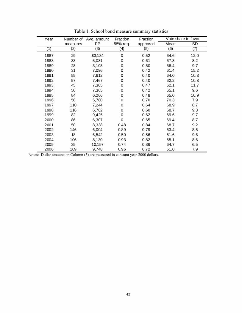
Table 1. School bond measure summary statistics

Mean SD(1) (2) (3) (4) (5) (6) (7)

1987 29 $3,134 0 0.52 64.6 12.01988 33 5,081 0 0.61 67.8 8.21989 28 3,103 0 0.50 66.4 9.71990 31 7,096 0 0.42 61.4 15.21991 55 7,612 0 0.40 64.0 10.31992 57 7,467 0 0.40 62.2 10.81993 45 7,305 0 0.47 62.1 11.71994 50 7,365 0 0.42 65.1 9.61995 84 6,266 0 0.48 65.0 10.91996 50 5,780 0 0.70 70.3 7.91997 110 7,244 0 0.64 68.9 8.71998 116 6,762 0 0.60 68.7 9.31999 82 9,425 0 0.62 69.6 9.72000 86 6,307 0 0.65 69.4 8.72001 50 8,338 0.48 0.84 68.7 9.22002 146 6,004 0.89 0.79 63.4 8.52003 18 6,542 0.50 0.56 61.6 9.62004 106 8,130 0.93 0.82 65.1 8.62005 35 10,157 0.74 0.86 64.7 6.52006 109 9,748 0.96 0.72 61.0 7.9

Year Fraction approved

Avg. amount PP

Vote share in favorNumber of measures

Fraction 55% req.

Notes: Dollar amounts in Column (3) are measured in constant year-2000 dollars.

42

Table 2. School district descriptive statistics for fiscal, housing markets and academic variables

All school Diff (4)-(5)disricts (t stat)

(1) (2) (3) (4) (5) (6)

Number of districts 948 319 629

A. Fiscal variablesNumber of observations 10,197 3,306 6,891 626 218

Log enrollment 7.43 6.18 8.03 8.34 8.09 0.25[1.69] [1.43] [1.47] [1.48] [1.48] (2.13)

Long term debt PP $1,984 479 2,706 1,736 1,247 489[3,286] [1,793] [3,581] [3,072] [2,388] (2.41)

Total expenditures PP $7,466 7,410 7,493 7,290 6,941 349[2,177] [2,293] [2,119] [1,898] [1,921] (2.32)

Capital outlays PP $922 679 1,038 882 935 -53[1,100] [905] [1,164] [1,005] [1,112] (0.62)

Current instructional $3,905 4,034 3,844 3,824 3,618 206expenditures PP [808] [941] [728] [703] [677] (3.82)

State and federal $4,520 4,958 4,309 4,242 4,223 20transfers PP [1,690] [1,791] [1,597] [1,564] [1,266] (0.18)

B. Housing market variablesNumber of observations 15,151 4,578 10,573 731 382

House prices $241,537 190,337 263,706 285,857 210,499 75,358[198,618] [149,691] [212,612] [240,439] [178,766] (5.91)

Log house prices 12.16 11.95 12.26 12.33 12.08 0.25[0.65] [0.62] [0.65] [0.66] [0.55] (6.71)

Square footage 1,603 1,572 1,615 1,625 1,637 -11[407] [456] [386] [401] [363] (0.47)

Lot size 56,772 97,604 39,797 32,342 49,388 -17,047[81,652] [111,614] [57,266] [48,933] [60,891] (4.73)

Sales volume 881 316 1,126 1,519 1,134 385[1,966] [951] [2,225] [3,568] [1,445] (2.54)

Income of homebuyers $96,482 84,753 101,674 107,689 90,339 17,350[59,094] [45,204] [63,606] [70,382] [58,903] (4.36)

Log income of homebuyers 11.36 11.25 11.40 11.45 11.31 0.14[0.46] [0.43] [0.47] [0.49] [0.41] (5.13)

C. Achievement variablesNumber of observations 9,748 3,240 6,508 460 170

Reading, grade 3 0.17 0.10 0.21 0.16 0.19 -0.028[0.91] [0.96] [0.88] [0.93] [0.81] (0.37)

Math, grade 3 0.07 -0.06 0.13 0.12 0.10 0.020[0.90] [0.99] [0.85] [0.88] [0.82] (0.27)

Never proposed a measure

Proposed at least one measure

Passed a measure (time t-1)

Failed a measure (time t-1)

Notes: Standard deviations in square brackets. In Column 6, bold coefficients are significant at the 5% level. Samples in Columns 1, 2 and 3 include all available observations in all years. Columns 4 and 5 include only observations for the year prior to a bond referendum. Fiscal variables are available for years 1995-2005, housing market variables for 1988 to 2005 (except income and log income, from 1992-2006), and test scores for 1992-1993 and 1997-2006. All dollar figures are measured in real year-2000 dollars. Achievement scores are standardized to mean zero and standard deviation one across schools in each year, then averaged to the district. Housing market variables are averages across transacted homes.

43

Table 3. Pre-bond measure balance of treatment and control groups

(1) (2) (3) (4) (5) (6) (7)

A. Fiscal OutcomesLong term debt PP 166 -607 -411 78 24 62 86

(201) (330) (312) (164) (61) (88) (86)Capital outlays PP -179 -220 -154 -44 0 54 95

(86) (133) (126) (145) (87) (121) (123)Current instructional exp. PP 91 -24 -12 35 -7 -6 -2

(44) (63) (62) (36) (19) (31) (31)State and federal transfers PP -139 -219 -202 187 147 193 223

(108) (160) (160) (143) (70) (129) (124)B. Housing market outcomesLog house prices 0.184 0.043 0.040 0.013 0.015 0.020 0.017

(0.029) (0.044) (0.043) (0.011) (0.007) (0.010) (0.010)C. Achievement outcomesReading, grade 3 -0.040 0.147 0.185 -0.010 -0.022 -0.032 -0.022

(0.088) (0.120) (0.117) (0.054) (0.034) (0.058) (0.057)Math, grade 3 0.042 0.180 0.214 0.054 -0.054 -0.002 0.004

(0.089) (0.112) (0.109) (0.062) (0.039) (0.059) (0.056)

Year effects & threshold control Y Y Y Y Y Y YCubic in vote share N Y Y Y N Y YSample pools relative years [-2, 6] N N Y Y N N YBond measure fixed effects N N N Y N N N

Year before election (t-1) Change, t-2 to t-1

Notes: Estimates in Columns 1-2 and 5-6 are estimated from cross-sectional data with observations for the year before a measure. Columns 3, 4, and 7 use a panel consisting of observations from two years before through six years after each election. The specification in Column 3 is that in equation (8). Column 4 uses equation (9), with only the effect of bond passage two years before the election constrained to zero; the effect of passage in the year before the election is reported . Models for house prices include controls for square footage, lot size and sales volume. Standard errors are clustered at the school district level. Bold coefficients are significant at the 5% level.

44

Table 4. The effect of bond passage on fiscal outcomes: Reduced-form and dynamic treatment effect estimates

1 yr later 2 yrs later 3 yrs later 4 yrs later 5 yrs later 6 yrs later(2) (3) (4) (5) (6) (7)

A. Reduced Form EffectsLong term debt PP 1,933 2,291 2,210 1,606 908 365

(360) (438) (473) (573) (612) (659)Capital outlays PP 255 802 1,121 841 219 -360

(151) (191) (244) (277) (276) (279)Current instructional 35 8 3 -26 -20 -19 expenditures PP (39) (43) (45) (56) (71) (74)State and federal transfers PP 100 41 -98 79 157 -13

(129) (149) (177) (175) (175) (193)B. Dynamic Treatment Effects

Recursive EstimatorLong-term debt PP 1,873 2,569 3,001 2,837 2,582 2,050

(388) (538) (660) (789) (873) (992)Capital outlays PP 250 822 1,303 1,281 924 381

(143) (193) (257) (308) (341) (372)Current instructional 44 13 1 -20 -20 -27 expenditures PP (41) (54) (59) (77) (100) (115)State and Federal Transfers PP 67 -22 -142 -19 11 -148

(120) (148) (190) (207) (227) (261)One-Step Estimator

Long-term debt PP 1,944 2,586 3,408 3,371 3,425 3,139(442) (563) (563) (619) (691) (689)

Capital outlays PP 220 792 1,549 1,660 1,091 554(157) (228) (299) (308) (268) (267)

Current instructional 22 -28 -33 -64 -80 -82 expenditures PP (46) (52) (49) (64) (77) (80)State and Federal Transfers PP 41 -50 184 104 91 -6

(133) (185) (311) (218) (203) (227) Notes: Dependent variables are measured in constant year-2000 dollars per pupil. Panel A presents estimates of the reduced-form coefficients on the bond passage indicator from equation (9) in the text. The sample consists of all bond elections and all outcome measures from years relative to the election -2 through +6. Some fiscal measures appear in the sample several times, for different relative years. N=6,970. Panel B presents estimates of the dynamic treatment effects, first using the "recursive" estimator and second using the "one-step" estimator. Both estimators are described in the text. Both are applied to the full panel of finance data, though only the effects of measure passage in years 1-6 are shown here. N=7,038. Standard errors in all specifications are clustered on the school district, and bold coefficients are significant at the 5% level.

45

Table 5. The effect of bond passage on log housing prices: Reduced-form and dynamic treatment effects

Reduced-Form Recursive One-Step

(1) (2) (3)Effect of measure passage in year of election 0.021 0.028 0.030

(0.015) (0.017) (0.017)Effect of measure passage 1 year later 0.027 0.041 0.036

(0.017) (0.021) (0.018)Effect of measure passage 2 years later 0.036 0.050 0.042

(0.020) (0.025) (0.020)Effect of measure passage 3 years later 0.058 0.077 0.062

(0.022) (0.030) (0.021)Effect of measure passage 4 years later 0.038 0.075 0.052

(0.024) (0.035) (0.022)Effect of measure passage 5 years later 0.038 0.086 0.054

(0.027) (0.041) (0.026)Effect of measure passage 6 years later 0.047 0.101 0.067

(0.035) (0.050) (0.034)R2 0.977 0.962

Dynamic Treatment Effects

Notes: Specifications are similar to those in Table 4 - see notes to that table for details. Specifications in this table include controls for square footage, lot size and sales volume. Number of observations is 8,016 (Column 1) and 10,313 (Columns 2-3). Dependent variable is the log of the mean sale price in the district, measured in 2000$. Bold coefficients are significant at the 5% level.

Table 6. Alternative specifications for fiscal outcomes and housing prices

(1) (2) (3) (4) (5) (6) (7) (8) (9)A. Fiscal outcomesLong term debt PP 3371 3733 3689 3371 -190 -542 1777 1787 3222

(619) (596) (583) (619) (382) (816) (984) (780) (558)Capital outlays PP 1660 1664 1586 1660 -234 82 544 1193 1546

(308) (268) (270) (308) (170) (307) (387) (449) (305)Curr. instr. expend. PP -64 -80 -65 -64 75 110 55 39 -69

(64) (58) (58) (64) (55) (93) (76) (72) (65)State/fed. transfers PP 104 210 127 104 -166 42 663 -33 76

(218) (198) (204) (218) (142) (264) (225) (308) (221)B. Housing outcomesLog prices 0.052 0.061 0.048 0.109 -0.078 0.031 -0.017 0.058

(0.022) (0.021) (0.024) (0.042) (0.033) (0.033) (0.034) (0.020)

Base (cubic)

3-part linearLinear

3-part cubic

Switch 55% & 67%

High capital

spending districts

Including parcel tax measures

Actual minus 10

Actual plus 10

Placebo thresholds

Notes: Column 1 presents one-step estimates of the effect of measure passage on outcomes four years later from the final rows of Table 4 and Column 3 of Table 5. Column 2 replaces the cubic in the vote share with a linear function; Column 3 uses separate linear segments in the [0, 55], [55, 66.7], and [66.7, 100] ranges; and Column 4 uses separate cubic segments in each range. Columns 5-7 include both the actual measure passage indicator and counterfactual indicators that reflect vote shares in excess of alternative thresholds; the coefficients shown are those on the counterfactual indicators. Column 8 reports estimates of the “reduced-form” effect on outcomes three years later, based on the subsample of measures where capital spending in the year before the election was above $562 per pupil, the median across all measures. Column 9 returns to the one-step estimator, and adds controls for the presence of a parcel tax measure on the ballot, a cubic in the parcel tax vote share, and an indicator for parcel tax passage, each interacted with relative year. Bold coefficients are significant at the 5% level.

46

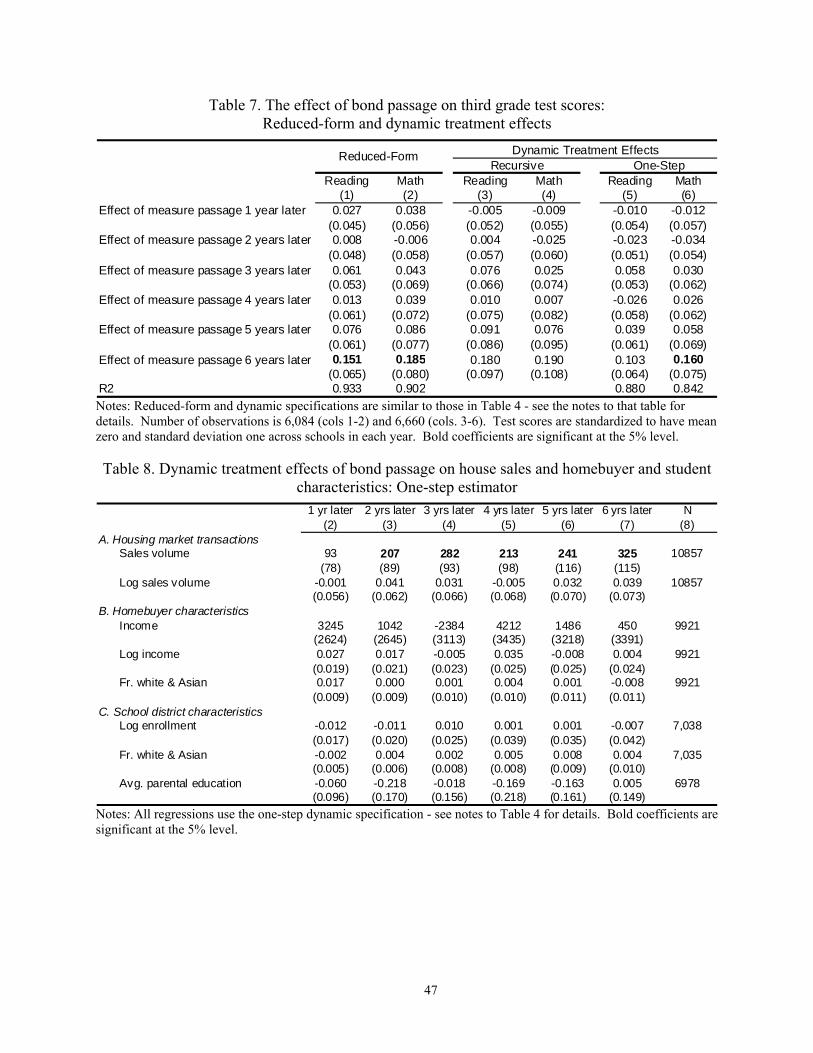
Table 7. The effect of bond passage on third grade test scores: Reduced-form and dynamic treatment effects

Reading Math Reading Math Reading Math(1) (2) (3) (4) (5) (6)

Effect of measure passage 1 year later 0.027 0.038 -0.005 -0.009 -0.010 -0.012(0.045) (0.056) (0.052) (0.055) (0.054) (0.057)

Effect of measure passage 2 years later 0.008 -0.006 0.004 -0.025 -0.023 -0.034(0.048) (0.058) (0.057) (0.060) (0.051) (0.054)

Effect of measure passage 3 years later 0.061 0.043 0.076 0.025 0.058 0.030(0.053) (0.069) (0.066) (0.074) (0.053) (0.062)

Effect of measure passage 4 years later 0.013 0.039 0.010 0.007 -0.026 0.026(0.061) (0.072) (0.075) (0.082) (0.058) (0.062)

Effect of measure passage 5 years later 0.076 0.086 0.091 0.076 0.039 0.058(0.061) (0.077) (0.086) (0.095) (0.061) (0.069)

Effect of measure passage 6 years later 0.151 0.185 0.180 0.190 0.103 0.160(0.065) (0.080) (0.097) (0.108) (0.064) (0.075)

R2 0.933 0.902 0.880 0.842

Dynamic Treatment EffectsRecursive One-Step

Reduced-Form

Notes: Reduced-form and dynamic specifications are similar to those in Table 4 - see the notes to that table for details. Number of observations is 6,084 (cols 1-2) and 6,660 (cols. 3-6). Test scores are standardized to have mean zero and standard deviation one across schools in each year. Bold coefficients are significant at the 5% level.

Table 8. Dynamic treatment effects of bond passage on house sales and homebuyer and student

characteristics: One-step estimator 1 yr later 2 yrs later 3 yrs later 4 yrs later 5 yrs later 6 yrs later N

(2) (3) (4) (5) (6) (7) (8)A. Housing market transactions

Sales volume 93 207 282 213 241 325 10857(78) (89) (93) (98) (116) (115)

Log sales volume -0.001 0.041 0.031 -0.005 0.032 0.039 10857(0.056) (0.062) (0.066) (0.068) (0.070) (0.073)

B. Homebuyer characteristicsIncome 3245 1042 -2384 4212 1486 450 9921

(2624) (2645) (3113) (3435) (3218) (3391)Log income 0.027 0.017 -0.005 0.035 -0.008 0.004 9921

(0.019) (0.021) (0.023) (0.025) (0.025) (0.024)Fr. white & Asian 0.017 0.000 0.001 0.004 0.001 -0.008 9921

(0.009) (0.009) (0.010) (0.010) (0.011) (0.011)C. School district characteristics

Log enrollment -0.012 -0.011 0.010 0.001 0.001 -0.007 7,038(0.017) (0.020) (0.025) (0.039) (0.035) (0.042)

Fr. white & Asian -0.002 0.004 0.002 0.005 0.008 0.004 7,035(0.005) (0.006) (0.008) (0.008) (0.009) (0.010)

Avg. parental education -0.060 -0.218 -0.018 -0.169 -0.163 0.005 6978(0.096) (0.170) (0.156) (0.218) (0.161) (0.149)

Notes: All regressions use the one-step dynamic specification - see notes to Table 4 for details. Bold coefficients are significant at the 5% level.

47

48

Appendix Table 1. One-step estimates of effect of bond passage on district balance sheet 1 yr later 2 yrs later 3 yrs later 4 yrs later 5 yrs later 6 yrs later

(1) (2) (3) (4) (5) (6)

Total revenues 288 458 899 741 657 667(201) (271) (479) (436) (450) (497)

Federal revenuse -5 -44 -73 -65 -58 -93(21) (26) (34) (32) (41) (46)

State revenues 46 -6 257 169 149 87(130) (185) (308) (211) (192) (215)

Local revenues 248 508 715 637 566 673(156) (220) (265) (356) (400) (427)

Loc. rev. - property tax collections 112 253 372 387 422 410(78) (159) (162) (313) (300) (321)

Loc. rev. - interest earned 44 127 123 110 74 84(23) (21) (35) (61) (61) (63)

Loc. rev. - all other 91 129 221 140 70 178(140) (129) (165) (108) (108) (139)

Total expenditures 198 853 1,688 1,841 1,169 701(188) (235) (337) (417) (374) (389)

Current elementary/secondary 3 -13 -6 12 -61 -49(68) (96) (105) (170) (168) (184)

Instructional 22 -28 -33 -64 -80 -82(46) (52) (49) (64) (77) (80)

Operation and maintenance of plant -25 -81 -84 -83 4 -13(35) (48) (54) (57) (53) (67)

Other 6 96 111 160 16 47(44) (59) (74) (130) (128) (137)

Non-elementary/secondary -42 -9 -22 0 16 17(24) (16) (18) (22) (26) (28)

Capital outlays 220 792 1,549 1,660 1,091 554(157) (228) (299) (308) (268) (267)

Intergovernmental payments 8 19 34 44 14 67(15) (35) (37) (58) (77) (83)

Interest on debt 9 65 132 125 108 112(13) (23) (27) (30) (33) (31)

Revenues minus expenditures 90 -395 -789 -1,100 -512 -35(185) (286) (324) (257) (282) (290)

Assets 1,852 2,455 2,601 2,088 1,671 1,376(549) (711) (612) (1,173) (1,110) (1,160)

Debt 1,941 2,572 3,420 3,369 3,442 3,159(442) (574) (565) (623) (695) (693)

Long term 1,944 2,586 3,408 3,371 3,425 3,139(442) (563) (563) (619) (691) (689)

Short term -3 -14 12 -2 17 20(10) (22) (8) (12) (11) (11)

Assets minus debt -89 -117 -819 -1,281 -1,771 -1,783(487) (527) (623) (1,189) (1,165) (1,251)

Notes: All regressions use the dynamic specification - see notes to Table 5 for details. All variables are measured in constant year-2000 dollars per pupil.