Embed Size (px)
Citation preview
NASA
Technical
Memorandum
NASA TM - 103591
, / .... . £'
/L"
...... / '-)
/,0 ,",I�I ....... /
(NASA-I_'-IO_5-_L)_,__, ., LINEAR ELASTIC
FRACTURe! t_LCHANICS PRIMER (NASA)
77 p
N92-30416
Unc I a s
GI_/39 0110792
LINEAR ELASTIC FRACTURE MECHANICS PRIMER
By C.D. Wilson
Structures and Dynamics Laboratory
Science and Engineering Directorate
July 1992
NASANational Aeronautics andSpace Administration
George C. Marshall Space Flight Center
MSFC-Form 3190 (Rev. May 1983)

PREFACE
Today's structural engineers are well-acquainted with using strength of materi-
als concepts and the finite element method for stress analysis. Additionally, most
structural engineers have a working knowledge of the fatigue behavior of metals. Un-
fortunately, the application of fracture mechanics is not as well understood. Fracture
analyses are often performed using computer software (NASA/FLAGRO [1] I and
NASCRAC [2] for example) as a "black box." This primer is intended to remove
the blackbox perception by introducing linear elastic fracture mechanics (LEFM) and
fracture control based on LEFM.
This primer began with the notes from two graduate courses at Tennessee Techno-
logical University: "Mechanics of High-Strength Materials" and "Fracture Mechan-
ics" taught by Dallas Smith of the Department of Civil Engineering. The author's
research interest in fracture mechanics was fostered by his graduate advisor, Dale
Wilson of the Department of Mechanical Engineering. After joining the George C.
Marshall Space Flight Center, the author was inspired by Gwyn Faile of the Durabil-
ity Analysis Branch to promote the development of fracture mechanics tools for the
practicing engineer. The notes from the course "SSME Fracture Mechanics," taught
by Dale Russell and his associates at the Rocketdyne Division of Rockwell Interna-
tional Corporation, were invaluable to the author. The author thanks Preston McGill
of the Metallurgy Research Branch and George Pinkas of Lewis Research Center for
the photographs used in this primer. The author also thanks the many people who
reviewed drafts of this primer.
C.D. Wilson
Huntsville, Alabama
July 1992
1The numbers in brackets refer to the list of references at the end of this paper.

TABLE OF CONTENTS
1 INTRODUCTION 1
1.1 Recommended Reading .......................... 1
1.2 Historical Perspective ........................... 1
1.3 Significance of Fracture Mechanics .................... 4
2 CRACK-TIP STRESSES 7
2.1 Modes of Crack-Tip Deformation .................... 7
2.2 Elastic Stress Field ............................. 8
2.3 Crack-Tip Plasticity ...... ..................... 10
3 STRESS INTENSITY FACTOR SOLUTIONS 14
3.1 Analytical Methods ............................ 14
3.2 Experimental Methods .......................... 16
3.3 Estimation Schemes ............................ 17
3.4 KI Solutions for Common Crack Geometries .............. 21
3.4.1 Through Cracks .......................... 21
3.4.2 Elliptical Embedded and Surface Cracks ............ 23
4 FRACTURE TOUGHNESS 27
4.1 Fracture Toughness Defined ....................... 27
4.2 Plane Strain Fracture Toughness Testing ................ 29
4.3 Plane Stress Fracture Toughness Testing ................ 32
SUBCRITICAL CRACK GROWTH 35
5.1 Fatigue Crack Growth .......................... 35
5.2 Sustained Load Crack Growth 42
6 DAMAGE TOLERANCE AND FRACTURE CONTROL 44
6.1 Philosophy and Basic Assumptions . .................. 44
6.2 Flaw-Screening Methods ......................... 46
6.2.1 Nondestructive Inspection .................... 46
6.2.2 Proof Testing ........................... 49
7 MISCELLANEOUS TOPICS 50
7.1 Relationship Between Kx and kt ..................... 50
7.2 Leak Before Burst ............................. 51
PRECED2'_G PAGE __AI',,K_OT F'_LMED
oo°
in
8 EXAMPLE PROBLEMS AND PRACTICE SET
8.1 Example Problems ............................
8.1.1
8.1.2
8.1.3
8.1.4
8.1.5
8.2
Stress Intensity Factor Calculation ...............
Factor of Safety for Critical Stress ................
Crack Growth in a Plate .....................
Flaw-screening Proof Test Factor ................
Solid Rocket Motor Case Failure ............... . .
Practice Set ................................
54
54
54
55
56
59
60
63
iv
LIST OF ILLUSTRATIONS
1 Griffith's flaw model ............................ 2
2 Engineering problem of a crack in a structure .............. 6
3 The three modes of crack-tip deformation ................ 7
4 Crack-tip stresses for mode I ....................... 9
5 First-order and second-order approximations of plastic zone ..... 11
6 FEM mesh for an edge crack in a plate .................. 15
7 Extrapolating for Kz using stress matching method ........... 15
8 Experimental fatigue crack growth method ............... 17
9 Superposition method ........................... 18
10 Compounding method ........................... 19
11 Weight function example ......................... 20
12 Embedded elliptical crack in an infinite body. ............. 25
13 Surface crack in a plate .......................... 25
14 Dependence of fracture toughness on thickness ............. 28
15 Compact tension fracture toughness specimen .............. 31
16 Types of load versus displacement plots from Kic tests ......... 31
17 Growth of a through crack in a thin plate ................ 33
18 Engineering estimate of residual strength ................ 33
19 Stress-cycle parameters in constant amplitude fatigue ......... 36
20 Fatigue crack growth rate as a function of AK ............. 36
21 _-AK for 7075-T6 aluminum alloy at room temperature. ...... 39
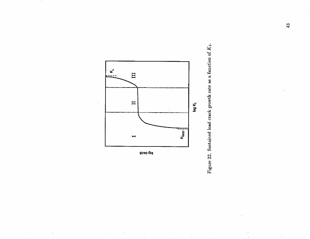
22 Sustained load crack growth rate as a function of KI .......... 43
23 Conservative LBB geometry. ....................... 52
24 Leak and burst regimes for R/t = 10 ................... 53
25 Fatigue crack growth of a center cracked plate .............. 58
26 Determination of proof factor for a center cracked plate ........ 61
27 Reassembled fragments from ruptured solid rocket motor case ..... 62
V
LIST OF TABLES
1
2
3
4
5
6
7
Conversions from English to SI units ................... 9
Elliptical integral of the second kind ................... 24
Surface crack tension correction factor (At) by Newman and Raju... 26
Surface crack bending correction factor (Ab) by Newman and Raju. 26
Typical yield strength and fracture toughness at room temperature. 29
Typical Paris equation constants for room temperature and R = 0... 38
Selected assumed initial flaw sizes from MSFC-STD-1249 ....... 48
vi
TECHNICAL MEMORANDUM
LINEAR ELASTIC FRACTURE MECHANICS PRIMER
1 INTRODUCTION
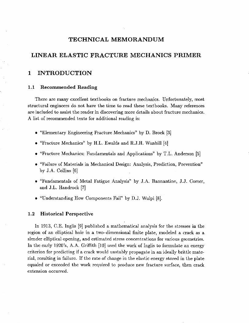
1.1 Recommended Reading
There are many excellent textbooks on fracture mechanics. Unfortunately, most
structural engineers do not have the time to read these textbooks. Many references
are included to assist the reader in discovering more details about fracture mechanics.
A list of recommended texts for additional reading is:
• "Elementary Engineering Fracture Mechanics" by D. Broek [3]
• "Fracture Mechanics" by H.L. Ewalds and R.J.H. Wanhill [4]
• "Fracture Mechanics: Fundamentals and Applications" by T.L. Anderson [5]
• "Failure of Materials in Mechanical Design: Analysis, Prediction, Prevention"
by J.A. Collins [6]
• "Fundamentals of Metal Fatigue Analysis" by J.A. Bannantine, J.J. Comer,
and J.L. Handrock [7]
• "Understanding How Components Fail" by D.J. Wulpi [8].
1.2 Historical Perspective
In 1913, C.E. Inglis [9] published a mathematical analysis for the stresses in the
region of an elliptical hole in a two-dimensional finite plate, modeled a crack as a
slender elliptical opening, and estimated stress concentrations for various geometries.
In the early 1920's, A.A. Griffith [10] used the work of Inglis to formulate an energy
criterion for predicting if a crack would unstably propagate in an ideally brittle mate-
rial, resulting in failure. If the rate of change in the elastic energy stored in the plate
equaled or exceeded the work required to produce new fracture surface, then crack
extension occurred.
2a << W
O
2a
= W =
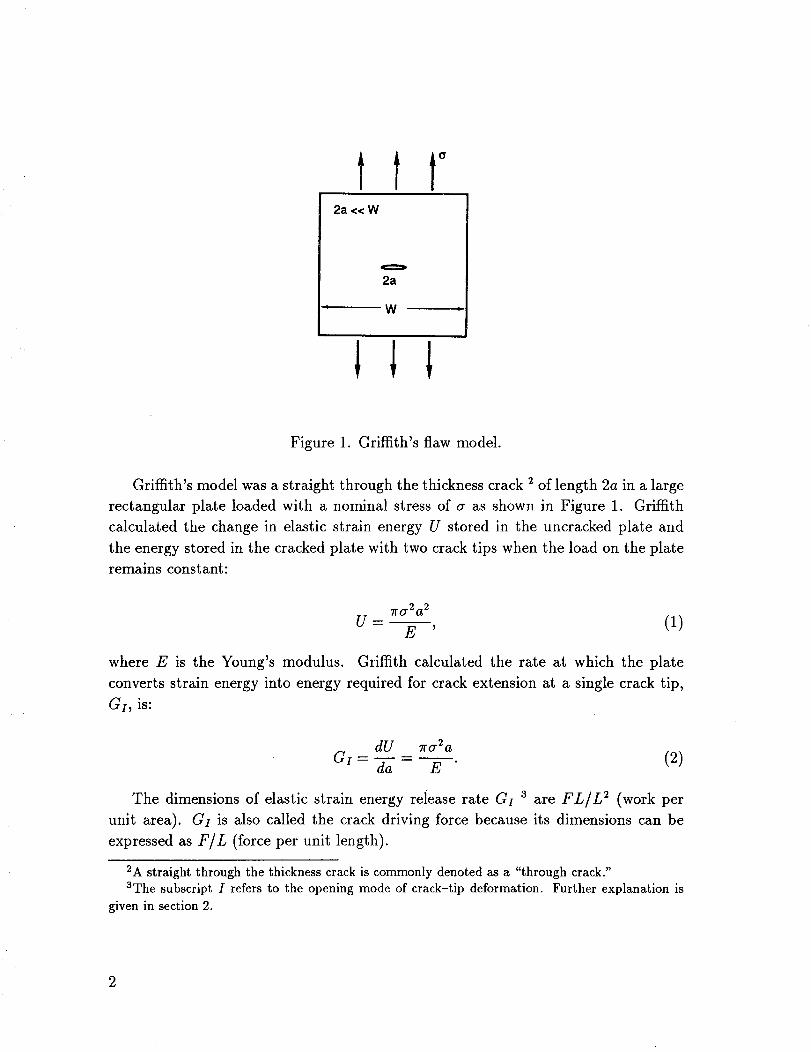
Figure 1. Griffith's flaw model.
Griffith's model was a straight through the thickness crack 2 of length 2a in a large
rectangular plate loaded with a nominal stress of a as shown in Figure 1. Griffith
calculated the change in elastic strain energy U stored in the uncracked plate and
the energy stored in the cracked plate with two crack tips when the load on the plate
remains constant:
7t-or2a 2
U- Z' (1)
where E is the Young's modulus. Griffith calculated the rate at which the plate
converts strain energy into energy required for crack extension at a single crack tip,
GI, is:
dU 7ro'2a
GI- da - E (2)
The dimensions of elastic strain energy release rate G_ 3 are FL/L 2 (work per
unit area). GI is also called the crack driving force because its dimensions can be
expressed as F/L (force per unit length).
2A straight through the thickness crack is commonly denoted as a "through crack."
3The subscript I refers to the opening mode of crack-tip deformation. Further explanation is
given in section 2.
2
As GI approaches a critical value Go, unstable crack extension is assumed to
occur. The critical stress can be determined by letting Gi _ Gc in equation 2 and
solving for ac:
crc = _/_ . (3)V _ra
The critical stress is proportional to a -1/2. The critical strain energy release rate Gc
is a constant for a given material and must be determined experimentally. Gc can be
viewed as the material's resistance to crack extension. In his experiments with glass,
Griffith assumed that the material's resistance was due to its surface energy 7, similar
to the surface tension of a liquid. Gc would be twice the surface energy (Go = 27)
because two new surfaces are formed during crack extension.
In the late 1940's, G.R. Irwin [11] and E. Orowan [12] showed that G_ for metals
is due to yielding and plastic deformation around the advancing crack tip rather than
surface energy. In fact, the surface energy for most metals is so small compared
with the plastic work that it can be neglected. Therefore, ignoring the plastic work
component of G_ severely underestimates the fracture strength of metals.
The energy approach has been largely replaced by a stress intensity factor (Ks) 4
approach developed by Irwin [13] and M.L. Williams [14] in the 1950's. Irwin showed
that fracture occurs when a critical stress distribution ahead of the crack tip is
reached. The stress intensity factor for the Griffith problem is:
K, = ax/_. (4)
There is a simple relationship between the stress intensity factor Ks approach and
the energy release rate G1 approach. Both sides of equation 4 are squared, and the
resulting expression is divided by E, and then combined with equation 2:
K/2 7ror2a- -c/. (5)E E
The above equation can be more generally stated:
C,=- K, (6)
4The stress intensity factor was denoted by the symbol K in honor of J.A. Kies, a collaborator of
Irwin's at the Naval Research Laboratory. The strain energy release rate was denoted by the symbol
G in honor of A.A. Griffith.
where E'= E for plane stress and E'= E/(1 - u 2) for plane strain _ (u is Poisson's
ratio). If Gi approaches its critical value, then Kz approaches its critical value.
P.C. Paris [15] applied fracture mechanics to the problem of fatigue in metals in
1961. He noted that the rate of fatigue crack growth was related to the stress intensity
factor range of the applied load cycles. By the early 1960's, fracture mechanics was
firmly established as a useful tool in preventing the failure of structures due to crack-
like defects.
1.3 Significance of Fracture Mechanics
The simplest way to establish the significance of the fracture mechanics approach
is to compare it to the strength of materials approach. In the strength of materials
approach, the applied stress is compared to the yield or ultimate strength of the
material. In the fracture mechanics approach, the applied stress must be combined
with an appropriate flaw size and then compared to the critical stress intensity factor.
For example, the critical pressure for a thin-walled pressure vessel can be determined
using both approaches. For the strength of materials approach, the hoop stress must
be less than the yield strength:
pR= T < ys. (7)
The critical pressure based on yield is:
For the fracture mechanics approach, the stress intensity factor, Kl, must be less
than the critical stress intensity factor, Kc:
pRKI = o'_r_ = _ _ < Kc.
t
The critical pressure based on fracture is:
(9)
P.fracture- V_
SThe terms "plane stress" and "plane strain" are explained in detail in section 2.3.
(lO)
4
where a is the largest flaw size that could exist undetected in the vessel. The fracture
mechanics approach governs the design when Pfr_,ct_,re < Pyietd. If this situation
occurs, ignoring fracture mechanics can easily lead to an unexpected failure.
Most structures contain defects or crack-like flaws. Structures made from brittle
materials are seriously affected because their strength is severely reduced by the stress
concentration near a crack. The high-strength, low-density metallic alloys used in
aerospace structures can be very flaw-sensitive. For this reason, fracture mechanics
was largely developed in the aerospace industry. However, its principles are widely
used in many other industries.
The possibility of brittle fracture occuring in a structure made from a high-
strength, flaw-sensitive material exists even when working stresses are well below
the yield strength. Brittle fracture from crack-like flaws can be catastrophic and
can occur with little advance warning, unlike ductile failure which usually requires
noticeable deformation and distortion. The crack-like flaws may originate from inclu-
sions and voids inherent in the material; fabrication processes like welding and heat
treatment; and mishandling of tools causing scratches or dents. Fatigue cracks can
initiate from these defects, as well as from other stress concentrations at fillets and
holes. Failures from brittle fracture have compelled engineers to design structures
which will tolerate flaws large enough to be detected by nondestructive inspection
before the flaws can grow to critical size.
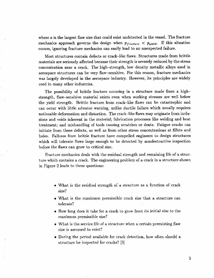
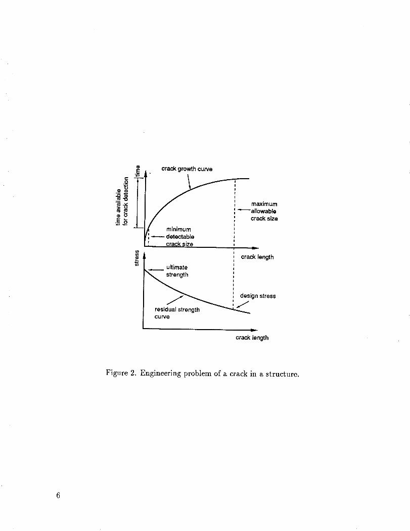
Fracture mechanics deals with the residual strength and remaining life of a struc-
ture which contains a crack. The engineering problem of a crack in a structure shown
in Figure 2 leads to these questions:
• What is the residual strength of a structure as a function of crack
size?
• What is the maximum permissible crack size that a structure can
tolerate?
• How long does it take for a crack to grow from its initial size to the
maximum permissible size?
• What is the service life of a structure when a certain preexisting flaw
size is assumed to exist?
• During the period available for crack detection, how often should a
structure be inspected for cracks? [3]
5
E,m
"°i==
o'J
crack growth curve
------ detectablecrack size
crack length
ultimate
design stress
curve
crack length
Figure 2. Engineering problem of a crack in a structure.
6
2 CRACK-TIP STRESSES
2.1 Modes of Crack-Tip Deformation
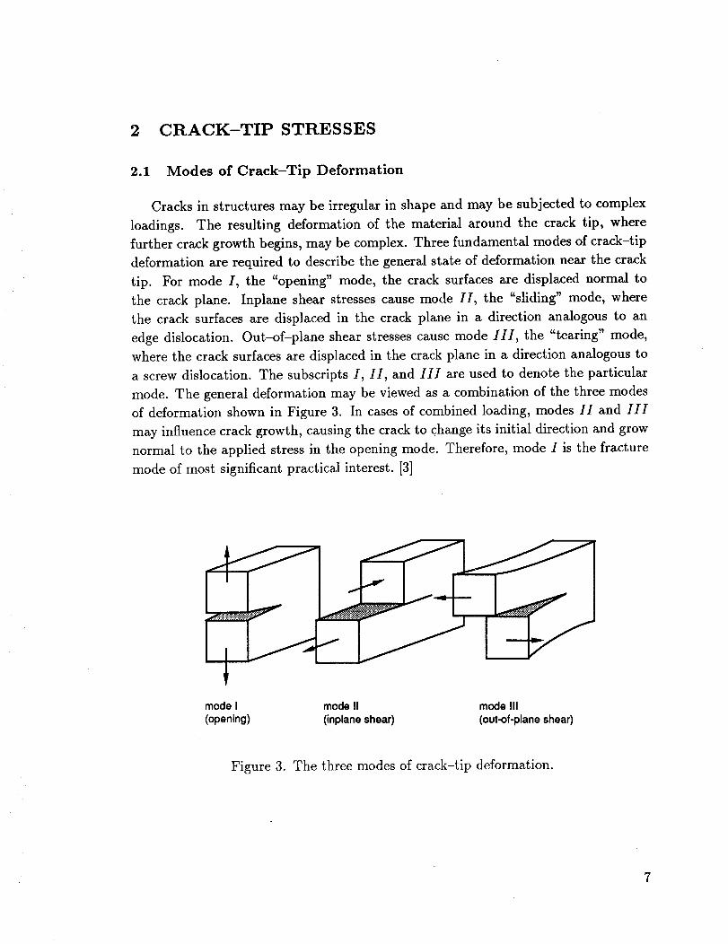
Cracks in structures may be irregular in shape and may be subjected to complex
loadings. The resulting deformation of the material around the crack tip, where
further crack growth begins, may be complex. Three fundamental modes of crack-tip
deformation are required to describe the general state of deformation near the crack
tip. For mode I, the "opening" mode, the crack surfaces are displaced normal to
the crack plane. Inplane shear stresses cause mode II, the "sliding" mode, where
the crack surfaces are displaced in the crack plane in a direction analogous to an
edge dislocation. Out-of-plane shear stresses cause mode III, the "tearing" mode,
where the crack surfaces are displaced in the crack plane in a direction analogous to
a screw dislocation. The subscripts I, II, and III are used to denote the particular
mode. The general deformation may be viewed as a combination of the three modes
of deformation shown in Figure 3. In cases of combined loading, modes II and III
may influence crack growth, causing the crack to change its initial direction and grow
normal to the applied stress in the opening mode. Therefore, mode I is the fracture
mode of most significant practical interest. [3]
fmode I mode II mode III
(opening) (inplane shear) (out-of-plane shear)
Figure 3. The three modes of crack-tip deformation.
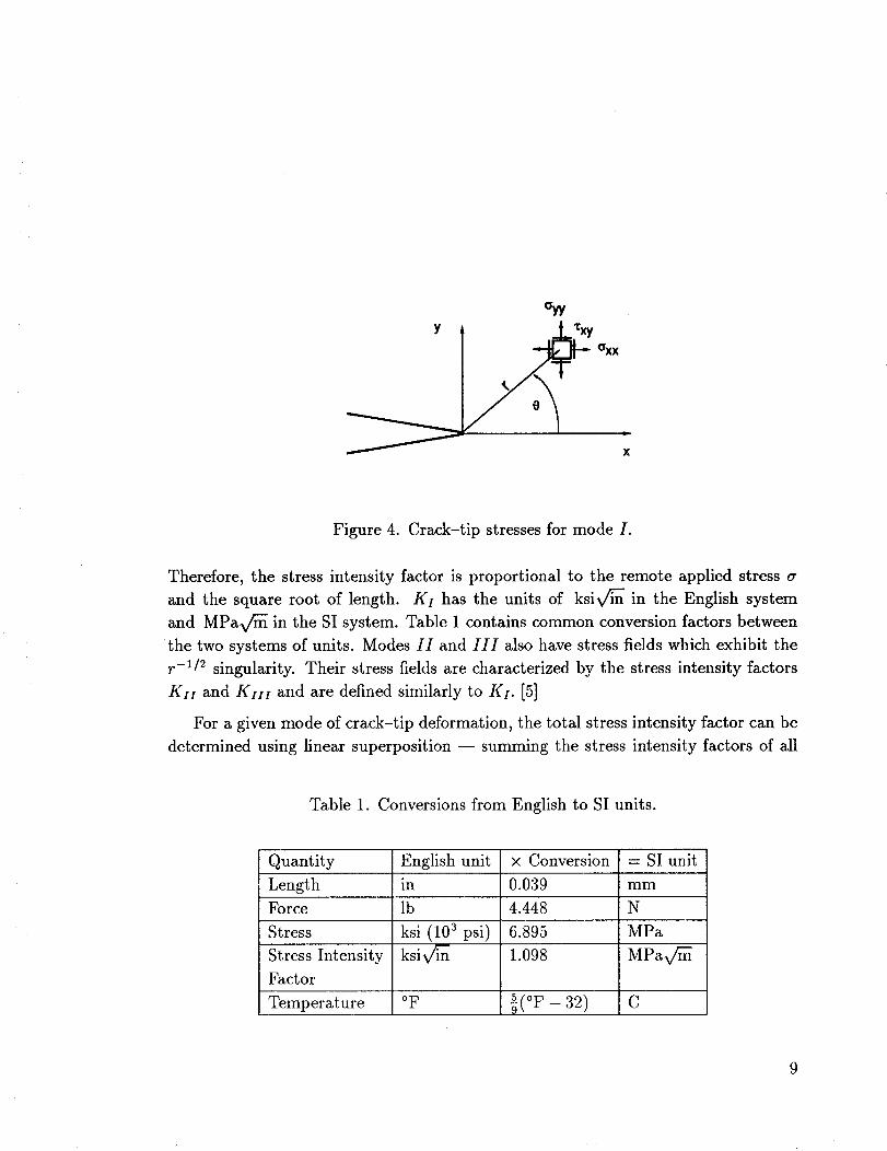
2.2 Elastic Stress Field
Irwin's stress intensity approach is based on the elastic stress field near the crack
tip. The stress components near the crack tip for mode I (Figure 4) have the form:
O'yy
O'ZZ
f 0 plane stress
u(o_x + ayy) plane strain,
where r is the distance from the crack tip, 0 is the angle of inclination, and K1 is
called the mode I stress intensity factor because its value governs the intensity of the
stress field. [3]
Along the line ahead of the crack (0 = 0):
KI
ax_ = aye= _, (11)
Txy _ O.
The crack-tip stresses of equation 11 are proportional to r -1/2, approaching infinity
as r approaches zero. The stresses for all mode I problems have the form given
by equation 11 regardless of boundary conditions and crack length. Kz changes its
value to reflect differences in boundary conditions, relative crack length, and crack
geometry.
The stress intensity factor is the basic parameter in LEFM because it controls the
magnitude of the stress singularity of equation 11. For a given specimen shape, crack
length, and the load, the stress intensity factor can usually be determined from a
handbook. For example, the stress intensity factor for the large cracked plate shown
in Figure 1 is:
KI = ax/_. (12)
8
Y
Figure 4. Crack-tip stresses for mode I.
Therefore, the stress intensity factor is proportional to the remote applied stress _r
and the square root of length. KI has the units of ksiv/_'ff in the English system
and MPav_ in the SI system. Table 1 contains common conversion factors between
the two systems of units. Modes II and III also have stress fields which exhibit the
r -1/2 singularity. Their stress fields are characterized by the stress intensity factors
KH and Kur and are defined similarly to KI. [5]
For a given mode of crack-tip deformation, the total stress intensity factor can be
determined using linear superposition -- summing the stress intensity factors of all
Table 1. Conversions from English to SI units.
Quantity English unit × Conversion = SI unit
Length in 0.039 mm
Force lb 4.448 N
MPaStress
Stress Intensity
Factor
Temperature
ksi (10 a psi)
ksiv/_
oF
6.895
1.098
I(°F-32)
MPav
C
loads acting to create that mode of deformation. Stress intensity factors from different
modes cannot be summed: Ktotat _ KI + KII + KHI. However, strain energy release
rates can be summed regardless of the mode of deformation: Gtotat = Gz+GH+GzII.
Using the relationships between G and K for each mode leads to:
K_ Kz21 (1 + u) K_I I (13)GtotaZ = --E-7 + --_ + E
The relationship between K1 and a for most geometries is more complicated than
the Griffith problem. In general, the stress intensity factor can be expressed:
K, = (14)
where _ s is the correction factor applied to the solution of the Griffith problem
(_ = 1) in Figure 1. The factor )_ depends on specimen geometry, relative crack
length and shape, and loading.
2.3 Crack-Tip Plasticity
The mathematical stress field contains infinite stresses at the crack tip. Certainly,
a real material cannot withstand infinite stresses. When the yield strength is exceeded
near the crack tip, a limited amount of plastic flow occurs. Therefore, the theoretically
infinite stresses are prevented by the presence of the crack-tip plastic zone shown
in Figure 5. Plasticity makes the crack behave as if it were longer than its actual
length because the crack-tip plastic zone results in larger crack-tip displacements and
reduced local stiffness. Irwin estimated the first-order (elastic) size of the plastic zone
by letting ayy in equation 11 equal the yield stress ays and solving for the distance
ry. For thin plates (whose constraint is referred to as plane stress):
1 (KII2 (15)ry = 2---_\ ay----_]
For thick plates (whose constraint is referred to as plane strain), an additional com-
ponent of stress, _rz_, inhibits plastic flow, making the plastic zone smaller by a factor
of three:
1 (IQI2 (16)ry = 6--_ \aye/
6_ expressions for several geometries are given in section 3.4.
10
--. Elastic
Elastic-Plastic
• i
: q.,,.
i.
r
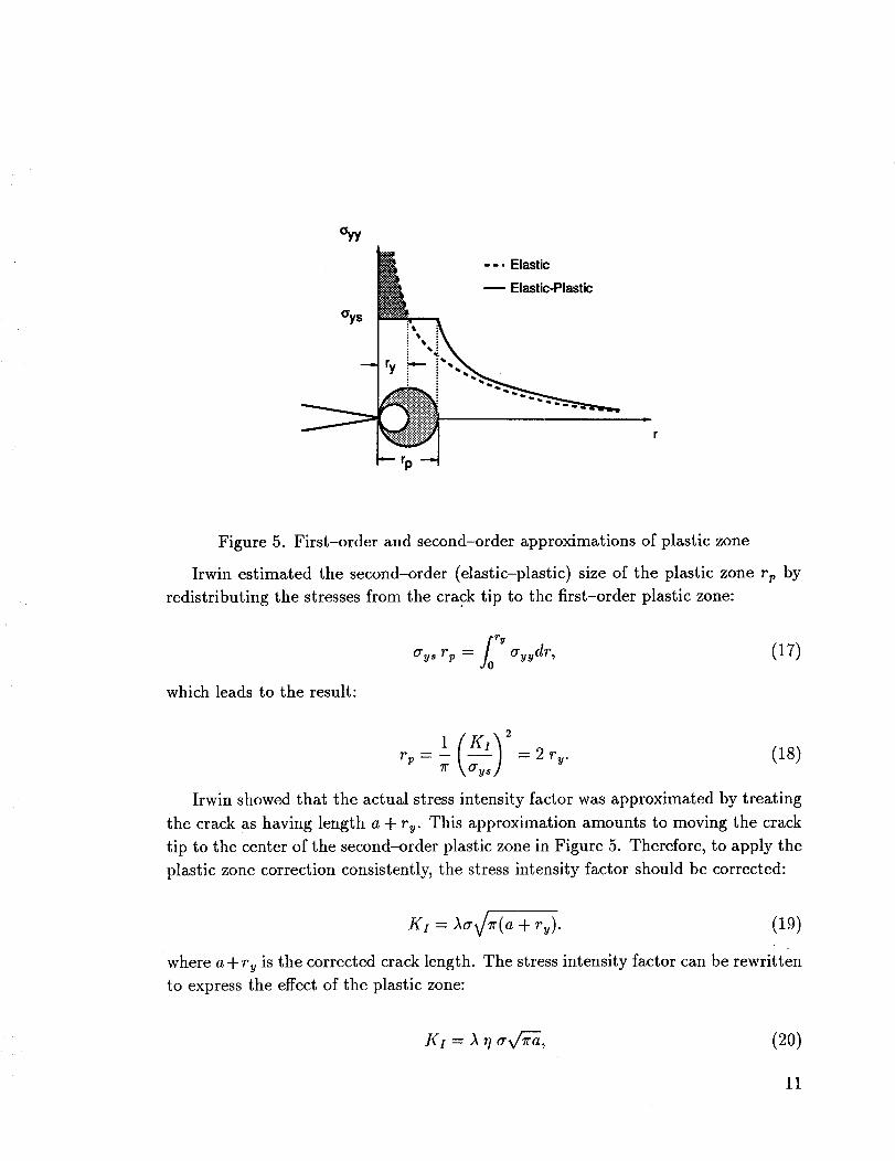
Figure 5. First-order and second-order approximations of plastic zone
Irwin estimated the second-order (elastic-plastic) size of the plastic zone vp by
redistributing the stresses from the crack tip to the first-order plastic zone:
which leads to the result:
_0 ryays r v = ayydr, (17)
r v = - = 2 ry. (18)
Irwin showed that the actual stress intensity factor was approximated by treating
the crack as having length a + ry. This approximation amounts to moving the crack
tip to the center of the second-order plastic zone in Figure 5. Therefore, to apply the
plastic zone correction consistently, the stress intensity factor should be corrected:
K,=_a¢_r(a+ry). (19)
where a + ry is the corrected crack length. The stress intensity factor can be rewritten
to express the effect of the plastic zone:
K, = , (20)
11
where7/is a factor representingthe increasein stressintensity due to the existenceof a plastic zone. 7/is a function of geometry, crack size, constraint, and ratio ofstress-to-yield strength:
1
where a = 2 for plane stressand a = 6 for plane strain. If the radicand in thedenominator of the aboveequation becomesless than zero, plastic zone instabilityoccurs. This condition representsthe limit of applicability of LEFM for monotonicloading.
If KI is expressed in a complicated manner, then r/may be difficult to determine
in closed form. In this case, iteration can be used to find the corrected KI, starting
with KI = )_a_-'ff as the initial guess. Usually, only three or four iterations are
required to achieve the desired convergence. A value for vy can be calculated after
KI is corrected.
Understanding the mechanics of crack-tip plasticity is very important. A state of
near-hydrostatic tension can exist at the crack tip; the tension is triaxial for plane
strain constraint or biaxial for plane stress contraint on an infinitesimal element. The
near-hydrostatic tension inhibits plastic flow which increases the tendency toward
brittle behavior. In thick plates, constraint varies from a triaxial state of stress in the
interior to a biaxial state of stress on the surface. A plate of intermediate thickness
has a plane stress plastic zone on the surface and has a plastic zone approaching the
condition of plane strain in the plate interior. Therefore, the dominant stress state
is difficult to determine for a plate of intermediate thickness. To estimate whether
the stress state is predominantly plane stress or plane strain, the following empirical
rules can be used:
• Plane stress is expected if the calculated plane stress plastic zone size 2ru is of
the order of the plate thickness.
• Plane strain is expected if the calculated plane stress plastic zone size 2ry is no
larger than ten percent of the plate thickness. [4]
The following criteria may be used to determine if a plastic zone correction should
be made:
12
a < 0.5ay,
0.5a_, < a _ 0.85ay,
0.85ay, < a
K I = Aa x/'_'ff,
gx = Aa_/r(a + rv),
elastic-plastic solution needed.
(22)
These criteria denote the limits of applicability of LEFM for monotonic loading.
Detailed models of crack-tip plastic zones can be found in References [3]-[5],
13
3 STRESS INTENSITY FACTOR SOLUTIONS
3.1 Analytical Methods
The finite element method (FEM) is a very powerful analytical technique that can
be used to determine crack tip displacements and stresses. Two simple approaches us-
ing FEM to determine stress intensity factors are the stress or displacement matching
approach and the energy approach. In the stress matching approach, K1 is determined
using extrapolated stresses or displacements (more accurate) near the crack tip. In
the energy approach, Kz is computed using its relationship to strain energy release
or compliance (inverse of stiffness).
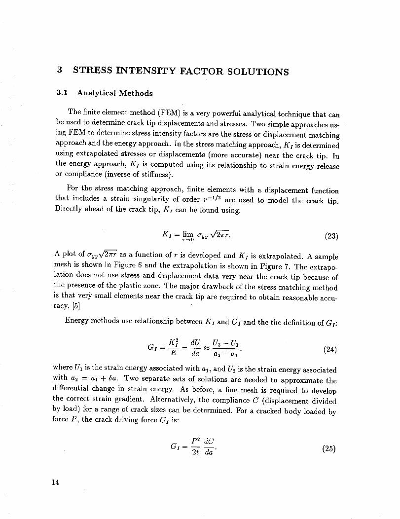
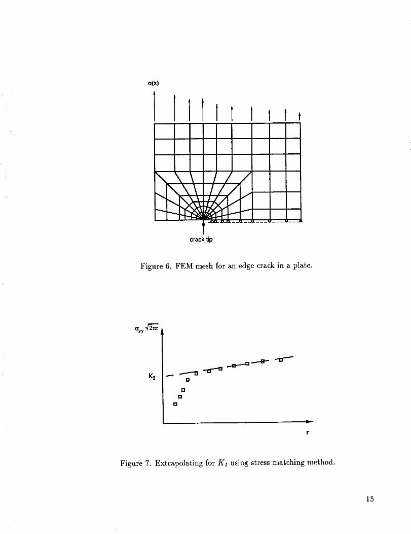
For the stress matching approach, finite elements with a displacement function
that includes a strain singularity of order r-l/2 are used to model the crack tip.
Directly ahead of the crack tip, K1 can be found using:
K1 = lim 2v/2_r.r--*O O'yy (23)
A plot of a_y 2_-7 as a function of r is developed and Kx is extrapolated. A sample
mesh is shown in Figure 6 and the extrapolation is shown in Figure 7. The extrapo-
lation does not use stress and displacement data very near the crack tip because of
the presence of the plastic zone. The major drawback of the stress matching method
is that very small elements near the crack tip are required to obtain reasonable accu-
racy. [5]
Energy methods use relationship between K1 and Gz and the the definition of GI:
K_ dU U2 - U_GI
= d---_-_ (24)a 2 -- a 1
where U1 is the strain energy associated with al, and/-/2 is the strain energy associated
with a2 = al + 5a. Two separate sets of solutions are needed to approximate the
differential change in strain energy. As before, a fine mesh is required to develop
the correct strain gradient. Alternatively, the compliance C (displacement divided
by load) for a range of crack sizes can be determined. For a cracked body loaded by
force P, the crack driving force GI is:
p2 gC
GI- 2t da" (25)
14
o(x)
II
\\1
I1 I tt,
///
crack tip
Figure 6. FEM mesh for an edge crack in a plate.
KI []
[][]
rl
r
Figure 7. Extrapolating for Kz using stress matching method.
15
The stress intensity factor can then be determined using the relationship between G1
and KI. [3, 5]
The use of FEM to solve fracture mechanics problems continues to be very active.
References [19]-[21] provide an updated overview of FEM-based fracture mechanics
and the special problems encountered when modeling cracks.
Another important method used to solve fracture mechanics problems is the
boundary integral equation method (BIEM). Unlike FEM, BIEM does not require
the meshing of the interior of a body. BIEM relies on the use of Betti's reciprocal
theorem which relates work done on a body by two distinct loadings. BIEM can be a
very efficient method for calculating stress intensity factors, but its use for nonlinear
problems is more difficult. [5, 22]
3.2 Experimental Methods
The use of strain gages on actual hardware is a very powerful technique for deter-
mining stress intensity factors. First, strain gages measure ex and % near the crack
tip. Then the stresses are computed using:
E
crxx - 1 - u 2 (e_ + u%),
E
ay_ - 1 - u 2 (% + vex).
The stress intensity factor is determined in the same manner as the FEM. Special care
must be taken to avoid placing the gage within the plastic zone. Additionally, the
size of the gage dictates that only rough estimates of stress intensity can be found. [3]
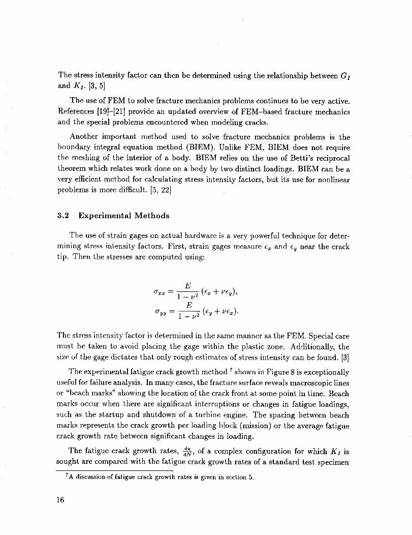
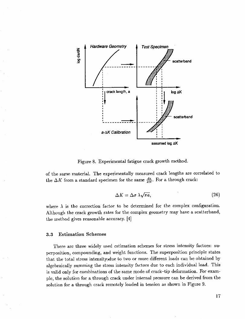
The experimental fatigue crack growth method 7 shown in Figure 8 is exceptionally
useful for failure analysis. In many cases, the fracture surface reveals macroscopic lines
or "beach marks" showing the location of the crack front at some point in time. Beach
marks occur when there are significant interruptions or changes in fatigue loadings,
such as the startup and shutdown of a turbine engine. The spacing between beach
marks represents the crack growth per loading block (mission) or the average fatigue
crack growth rate between significant changes in loading.
da of a complex configuration for which KI isThe fatigue crack growth rates, _W,
sought are compared with the fatigue crack growth rates of a standard test specimen
7A discussion of fatigue crack growth rates is given in section 5.
16
Z
o
Hardware Geometry
I
,,
, =
Test Specimen
scatterband
! I
I I
i I I ___!
',I cracklength,a " I log AK
'1 '1! I
I ;.;.;.;.., , t#i:/i i ,':."I_I_P
, ' l ..:_i_i::'1 : _scatterband
; ....... ......../" II
I i
! I
assumedlogAK
Figure 8. Experimental fatigue crack growth method.
of the same material. The experimentally measured crack lengths are correlated to
as For a through crack:the AK from a standard specimen for the same _--#.
where $ is the correction factor to be determined for the complex configuration.
Although the crack growth rates for the complex geometry may have a scatterband,
the method gives reasonable accuracy. [4]
3.3 Estimation Schemes
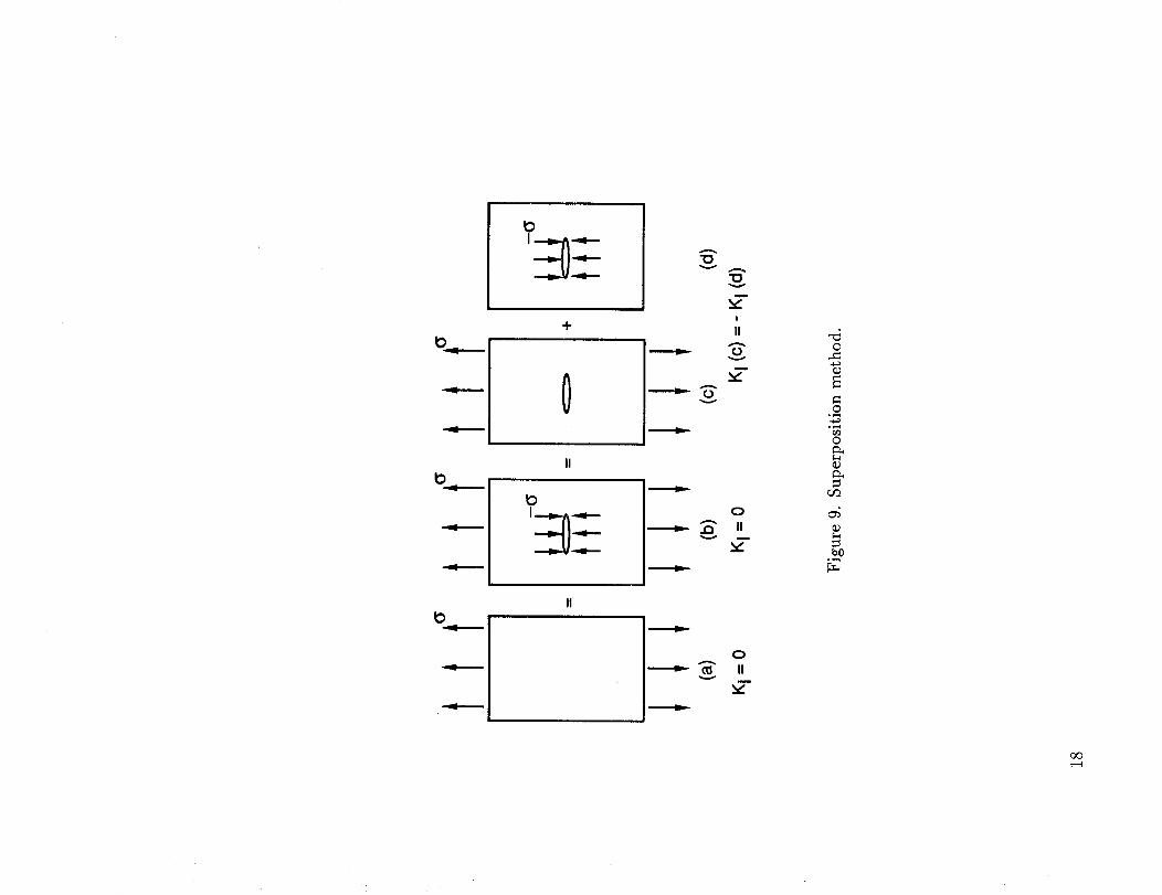
There are three widely used estimation schemes for stress intensity factors: su-
perposition, compounding, and weight functions. The superposition principle states
that the total stress intensity_ue to two or more different loads can be obtained by
algebraically summing the stress intensity factors due to each individual load. This
is valid only for combinations of the same mode of crack-tip deformation. For exam-
ple, the solution for a through crack under internal pressure can be derived from the
solution for a through crack remotely loaded in tension as shown in Figure 9.
17
4-
0
A
v
v
m
!
IIA
v
',t
v
0
.D IIm
O
a_ II
o
o
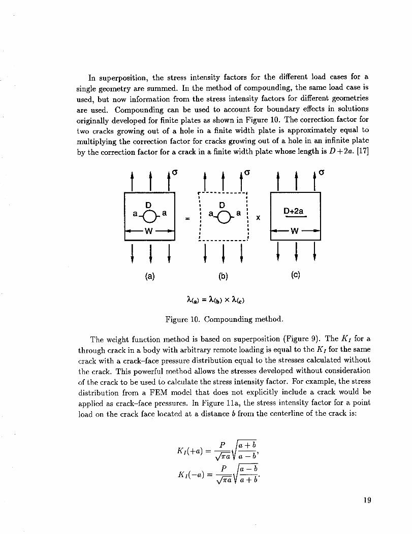
In superposition, the stress intensity factors for the different load cases for a
single geometry are summed. In the method of compounding, the same load case is
used, but now information from the stress intensity factors for different geometries
are used. Compounding can be used to account for boundary effects in solutions
originally developed for finite plates as shown in Figure 10. The Correction factor for
two cracks growing out of a hole in a finite width plate is approximately equal to
multiplying the correction factor for cracks growing out of a hole in an infinite plate
by the correction factor for a crack in a finite width plate whose length is D + 2a. [17]
D
"-- W "-'_
(a)
ttt°D
a.. a
(b)
×D+2a
,_---- W .-_,*
(c)
_'(a)= _'(b)X _,(c)
Figure 10. Compounding method.
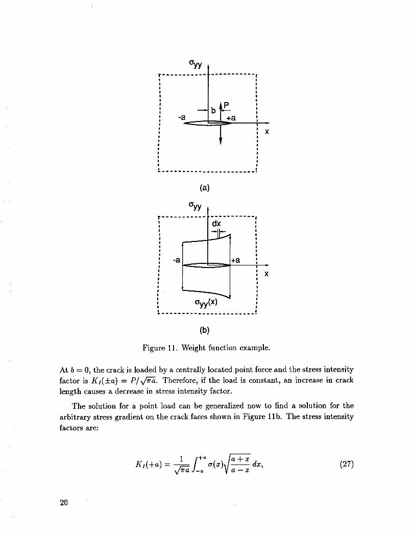
The weight function method is based on superposition (Figure 9). The Kt for a
through crack in a body with arbitrary remote loading is equal to the KI for the same
crack with a crack-face pressure distribution equal to the stresses calculated without
the crack. This powerful method allows the stresses developed without consideration
of the crack to be used to calculate the stress intensity factor. For example, the stress
distribution from a FEM model that does not explicitly include a crack would be
applied as crack-face pressures. In Figure lla, the stress intensity factor for a point
load on the crack face located at a distance b from the centerline of the crack is:
Ki(+a) -
Ki(-a) -
-b'
P _-a -b
19
Oyy
-a
!
X
(a)
Oyy
dx
-a _ _-a
Oyy(X)|
X
(b)
Figure 11. Weight function example.
At b = 0, the crack is loaded by a centrally located point force and the stress intensity
factor is K,(+a) = P/vr_'-6. Therefore, if the load is constant, an increase in crack
length causes a decrease in stress intensity factor.
The solution for a point load can be generalized now to find a solution for the
arbitrary stress gradient on the crack faces shown in Figure 11b. The stress intensity
factors are:
1 a x a + x (27)K , (+ a ) - v/_-._ _ _' ( ) _dx,
20
1 J+_a(x) a-Xdx.K i ( - a ) - v/=_ aa_ x (28)
If o'(x) = P, then the above equations reduce to the case of uniform pressure on the
crack faces: gl(4-a) = Pv/'_. [4]
For an uncracked stress field that can be approximated using a second-order
polynomial, o" = o'r<f(Co + ClX + C2x2), the stress intensity factors for a through
crack centered in an infinite plate are:
a a 2
gx(+a) : (Co + C1-_ + C2-_-)(rr_fv/_, (29)
a a 2
Ki(-a) = (C0 - C,_ -t- C2-_--) ¢rreIV_. (30)
For higher-order polynomials, numerical integration should be used to determine Kx.
Methods for obtaining stress intensity factor solutions using this method can be found
in Reference [18].
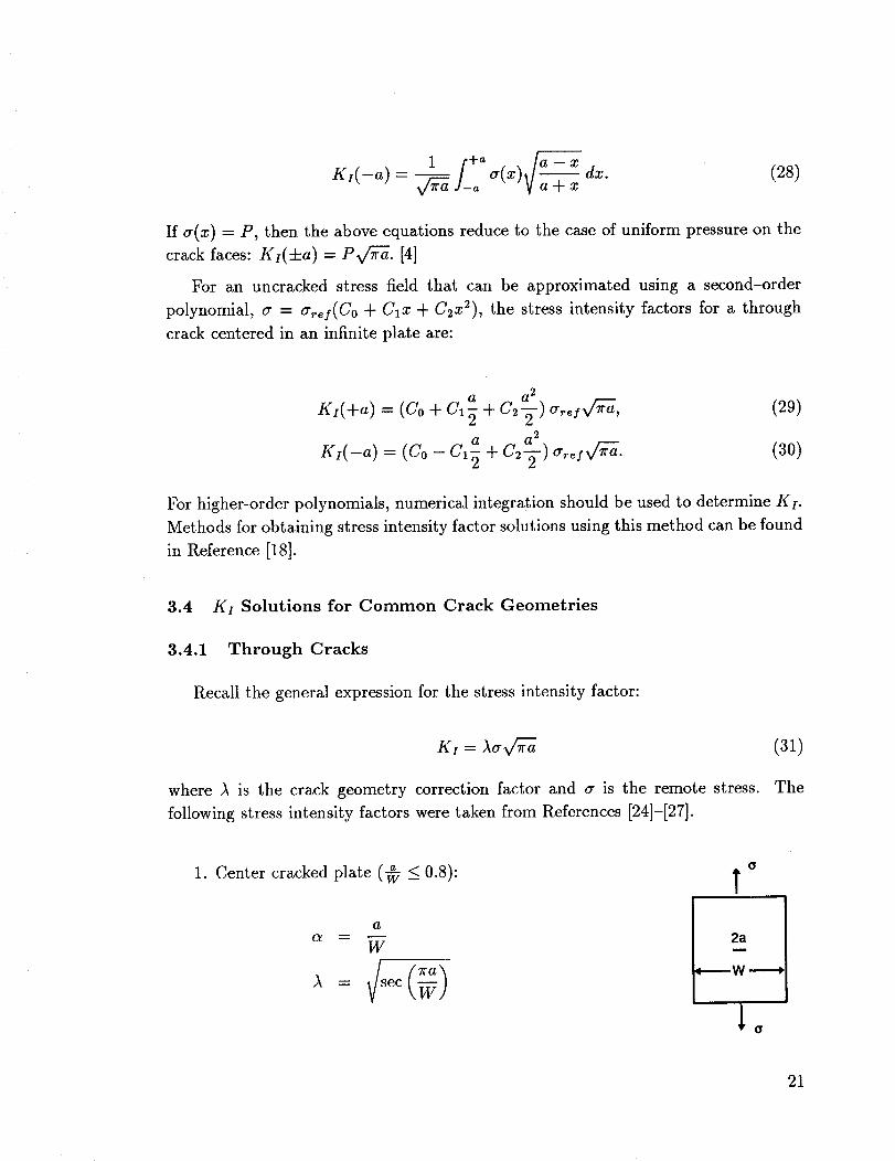
3.4 Kx Solutions for Common Crack Geometries
3.4.1 Through Cracks
Recall the general expression for the stress intensity factor:
gr = Aav/_ (31)
where A is the crack geometry correction factor and a is the remote stress. The
following stress intensity factors were taken from References [24]-[27].
1. Center cracked plate (w -< 0.8):
a
W
o
!
2a
21
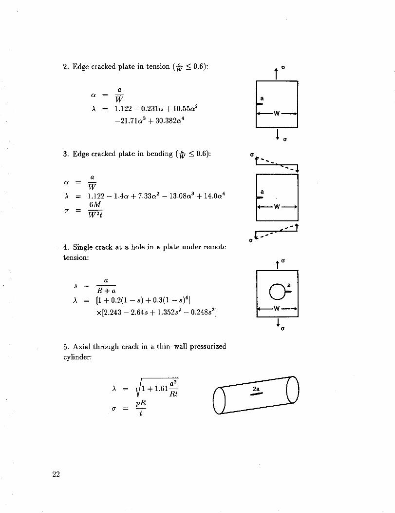
2. Edgecrackedplate in tension (_ _<0.6):
a
W
)_ = 1.122 - 0.231c_ + 10.55c_ 2
-21.71c_ a + 30.382c_ 4
3. Edge cracked plate in bending (_ _< 0.6):
acl_ = m
W
)_ = 1.122 - 1.4a + 7.33a 2 - 13.08a a ÷ 14.0a 4
6MO" --
W2t
4. Single crack at a hole in a plate under remote
tension:
=
a
R+a
[1 + 0.2(1 - s) + 0.3(1 - s) n]
×[2.243 - 2.64s + 1.352s 2 - 0.248s 3]
{$
T
aD
4"--'-" W -------_
I O
aD
_----- W --------_
5. Axial through crack in a thin-wall pressurized
cylinder:
_/ a2)_ = 1 + 1.61R---)--
pR6r --
t
22
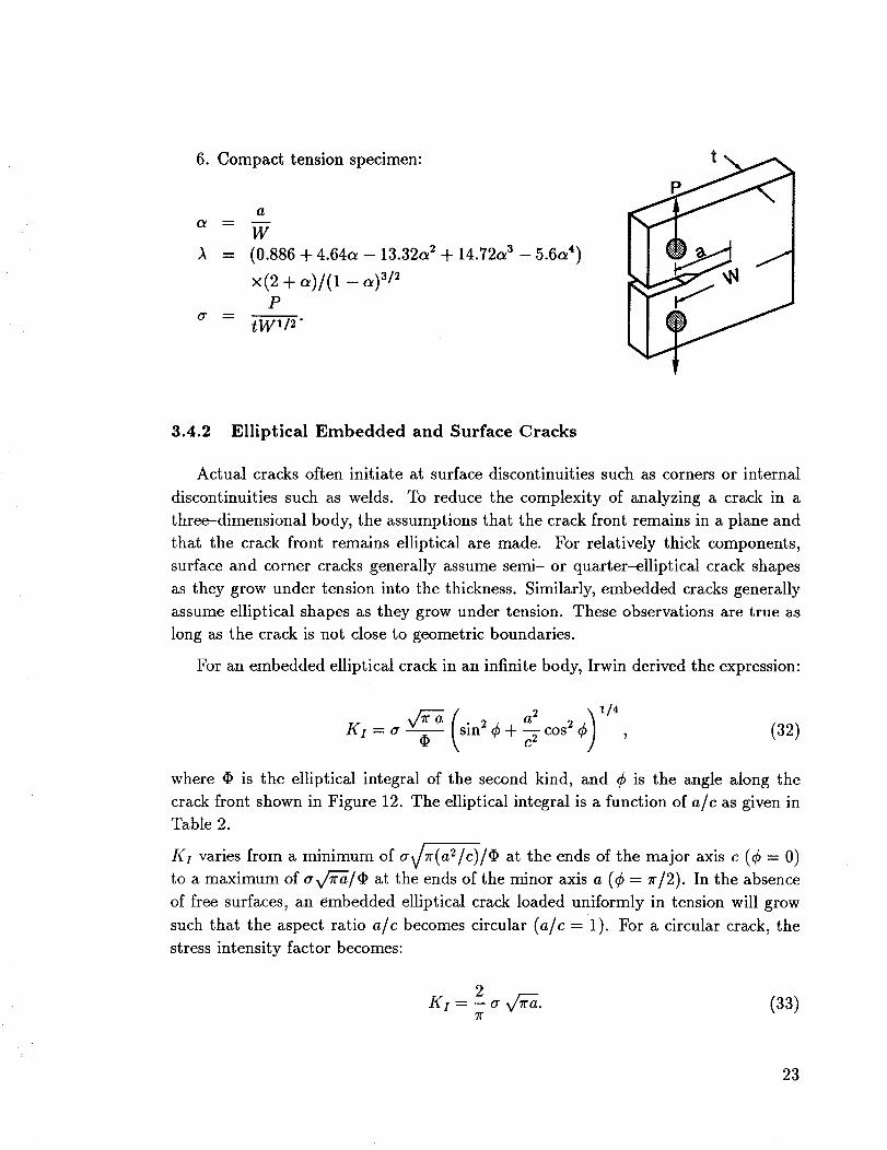
6. Compacttension specimen:
a
W
A = (0.886 + 4.64a - 13.32_ 2 + 14.72c_ 3 - 5.6a 4)
x(2 + .)/(i -P
(7tW1/2 •
3.4.2 Elliptical Embedded and Surface Cracks
Actual cracks often initiate at surface discontinuities such as corners or internal
discontinuities such as welds. To reduce the complexity of analyzing a crack in a
three--dimensional body, the assumptions that the crack front remains in a plane and
that the crack front remains elliptical are made. For relatively thick components,
surface and corner cracks generally assume semi- or quarter-elliptical crack shapes
as they grow under tension into the thickness. Similarly, embedded cracks generally
assume elliptical shapes as they grow under tension. These observations are true as
long as the crack is not close to geometric boundaries.
For an embedded elliptical crack in an infinite body, Irwin derived the expression:
rv/_-_ (sin2 a2 )1/4It', = or _ ¢ + _ cos 2 ¢ , (32)
where • is the elliptical integral of the second kind, and ¢ is the angle along the
crack front shown in Figure 12. The elliptical integral is a function of a/c as given in
Table 2.
IQ varies from a minimum of a_/_r(a2/c)/_ at the ends of the major axis c (¢ = 0)
to a maximum of orv'ff"d/¢ at the ends of the minor axis a (¢ = 7r/2). In the absence
of free surfaces, an embedded elliptical crack loaded uniformly in tension will grow
such that the aspect ratio a/c becomes circular (a/c = 1). For a circular crack, the
stress intensity factor becomes:
2Kx = - a x/_. (33)
71"
23
For a surfacecrack, Irwin estimatedthat the presenceof the front free surfaceofa semi-elliptical crack could be accountedfor by compoundingthe correction factorfor the embeddedcrack in an infinite body with the the correction factor for a smalledgecrack in a plate:
K1 = 1.12 2- a x/_. (34)lr
If the crack intersects two front surfaces, such as a quarter-elliptical crack, then a
correction factor of 1.2 should be used. If the surface or corner crack grows deeper
than half the plate thickness, then a back surface correction factor must be used. This
back surface correction is analogous to the correction factor for finite width effects
for a through crack in a plate.
More accurate solutions based on finite element results for semi-elliptical cracks
are given by J.C. Newman, Jr. and I.S. Raju. [28]-[30] Their solution for a flat plate
loaded in tension and bending (Figure 13) is in the form:
K, = +
with )_t given in Table 3, )% given in Table 4, and _, given by:
(35)
is ( c,ff_ (36))_'= eCkwv t ]"
Table 2. Elliptical integral of the second kind.
a/c ¢ a/c ¢
0.1 1.0160 0.6 1.2763
0.2 1.0505 0.7 1.3456
0.3 1.0965 0.8 1.4181
0.4 1.1507 0.9 1.4933
0.5 1.2111 1.0 1.5708
24
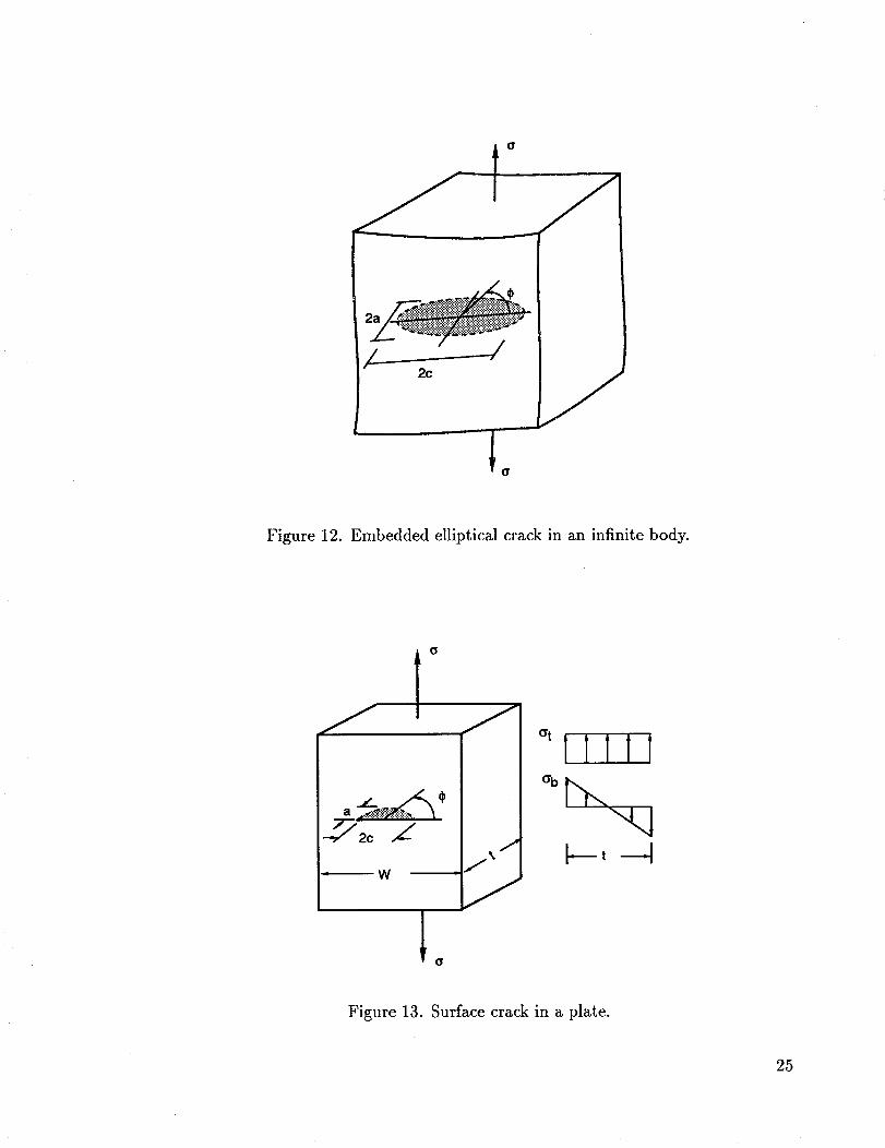
l °
2c
Figure 12. Embedded elliptical crack in an infinite body.
----------- W
Figure 13. Surface crack in a plate.
25
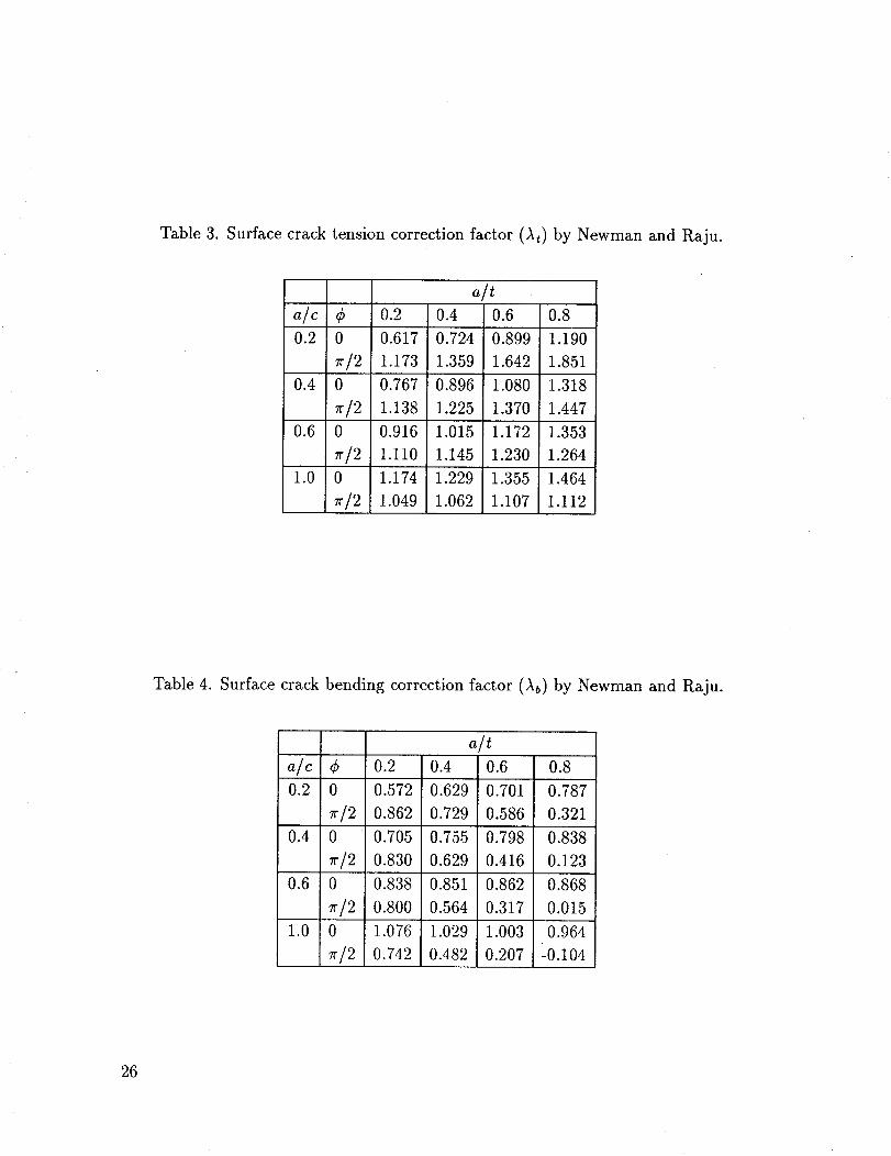
Table 3. Surfacecracktension correctionfactor (At) by Newmanand Raju.
a/ta/c ¢ 0.2 0.4 0.6 0.8
0.2 0 0.617 0.724 0.899 1.190
7r/2 1.173 1.359 1.642 1.851
0.4 0 0.767 0.896 1.080 1.318
7r/2 1.138 1.225 1.370 1.447
0.6 0 0.916 1.015 1.172 1.353
_'/2 1.110 1.145 1.230 1.264
1_.0 0 1.174 1.229 1.355 1.464
7r/2 1.049 1.062 1.107 1.112
Table 4. Surface crack bending correction factor (_b) by Newman and Raju.
a/ta/c ¢ 0.2 0.4 0.6 0.8
0.2 0 0.572 0.629 0.701 0.787
_r/2 0.862 0.729 0.586 0.321
0.4 0 0.705 0.755 0.798 0.838
_-/2 0.830 0.629 0.416 0.123
0.6 0 0.838 0.851 0.862 0.868
r/2 0.800 0.564 0.317 0.015
1.0 0 1.076 1.029 1.003 0.964
7r/2 0.742 0.482 0.207:0.104
26
4 FRACTURE TOUGHNESS
4.1 Fracture Toughness Defined
Fracture toughness is defined as the material's critical stress intensity factor.
While regarded as a material property, the fracture toughness of a given material
may be strongly affected by operating temperature, heat treatment, and constraint
(plate thickness). Therefore, care must be taken in design to use a value of frac-
ture toughness which closely simulates the expected operating temperature and any
corrosive environments present.
Constraint changes with plate thickness and strongly affects fracture toughness.
Near the crack tip in thick plates," azz develops normal to the plate surfaces. A
state of triaxial tension (plane strain) exists in the material near the crack tip. The
additional constraint inhibits plastic flow of material around the crack tip, promoting
brittle behavior. In thinner plates, az_ exists to a lesser degree and more plastic flow
occurs at the crack tip, dulling the crack tip and producing an apparent increase in
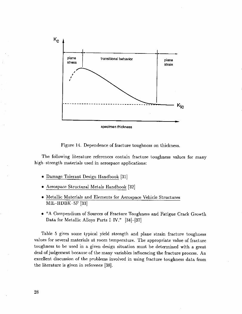
fracture toughness. As plate thickness is increased, the critical stress intensity factor
eventually approaches a lower bound as indicated in Figure 14. This lower bound
value is called the plane strain fracture toughness, and the symbol Krc is reserved for
this material property.
Operating temperature also strongly affects fracture toughness. As temperature
decreases, the fracture toughness tends to decrease. For example, 4340 steel has a
fracture toughness of 50 ksix/_ at 75°F, but the toughness drops to 30 ksiv_ at
-100°F. Therefore, fracture toughness is a material property that can vary consid-
erably with temperature.
Fracture toughness can be used in the material selection process to screen can-
didate materials. One criterion for using fracture toughness that will ensure plane
stress or high energy failure is:
K,c >_ aysx/_, (37)
where t is the plate thickness. If this inequality can be achieved, then the design will
be relatively insensitive to low energy failure due to crack-like defects. [4]
27
Kc
plane transitional behaviorstress
I
#l I
planestrain
KIc
specimenthickness
Figure 14. Dependence of fracture toughness on thickness.
The following literature references contain fracture toughness values for many
high-strength materials used in aerospace applications:
® Damage Tolerant Design Handbook [31]
* Aerospace Structural Metals Handbook [32]
. Metallic Materials and Elements for Aerospace Vehicle Structures
MIL-HDBK-5F [33]
• "A Compendium of Sources of Fracture Toughness and Fatigue Crack Growth
Data for Metallic Alloys Parts I-IV." [34]-[37]
Table 5 gives some typical yield strength and plane strain fracture toughness
values for several materials at room temperature. The appropriate value of fracture
toughness to be used in a given design situation must be determined with a great
deal of judgement because of the many variables influencing the fracture process. An
excellent discussion of the problems involved in using fracture toughness data from
the literature is given in reference [38].
28
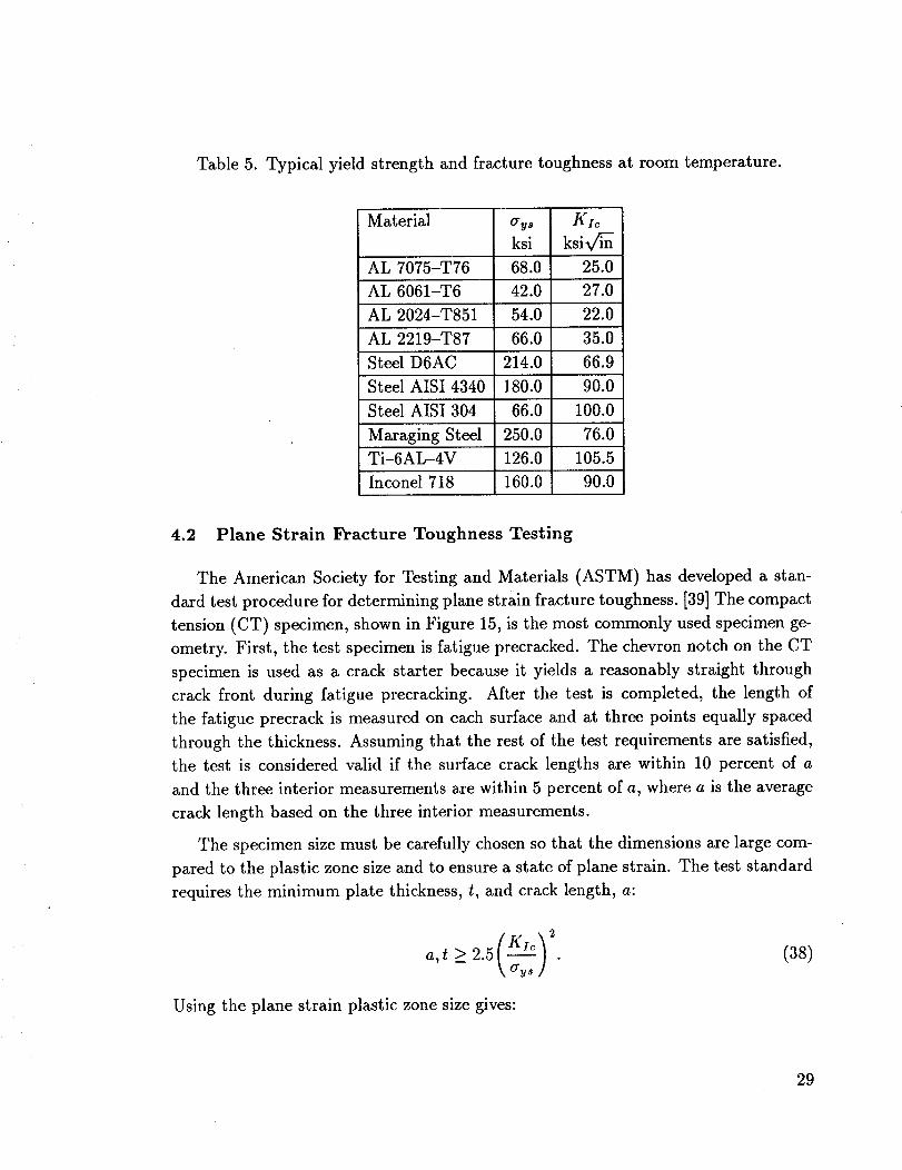
Table 5. Typical yield strength and fracture toughness at room temperature.
Material
AL 7075-T76
AL 6061-T6
AL 2024-T851
AL 2219-T87
Steel D6AC
Steel AISI 4340
Steel AISI 304
Maraging Steel
Ti-6AL-4V
Inconel 718
av, KIc
ksi ksiv_
68.0 25.0
42.0 27.0
54.0 22.0
66.0 35.0
214.0 66.9
180.0 90.0
66.O 100.0
250.0 76.0
126.0 105.5
160.0 90.0
4.2 Plane Strain Fracture Toughness Testing
The American Society for Testing and Materials (ASTM) has developed a stan-
dard test procedure for determining plane strain fracture toughness. [39] The compact
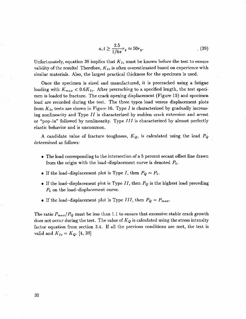
tension (CT) specimen, shown in Figure 15, is the most commonly used specimen ge-
ometry. First, the test specimen is fatigue precracked. The chevron notch on the CT
specimen is used as a crack starter because it yields a reasonably straight through
crack front during fatigue precracking. After the test is completed, the length of
the fatigue precrack is measured on each surface and at three points equally spaced
through the thickness. Assuming that the rest of the test requirements are satisfied,
the test is considered valid if the surface crack lengths are within 10 percent of a
and the three interior measurements are within 5 percent of a, where a is the average
crack length based on the three interior measurements.
The specimen size must be carefully chosen so that the dimensions are large com-
pared to the plastic zone size and to ensure a state of plane strain. The test standard
requires the minimum plate thickness, t, and crack length, a:
\ey_ /
Using the plane strain plastic zone size gives:
29
2.5a,t >_ 1-_ry _ 50ry. , (39)
Unfortunately, equation 38 implies that Kzc must be known before the test to ensure
validity of the results! Therefore, Kic is often overestimated based on experience with
similar materials. Also, the largest practical thickness for the specimen is used.
Once the specimen is sized and manufactured, it is precracked using a fatigue
loading with Kma_ < 0.6KI_. After precracking to a specified length, the test speci-
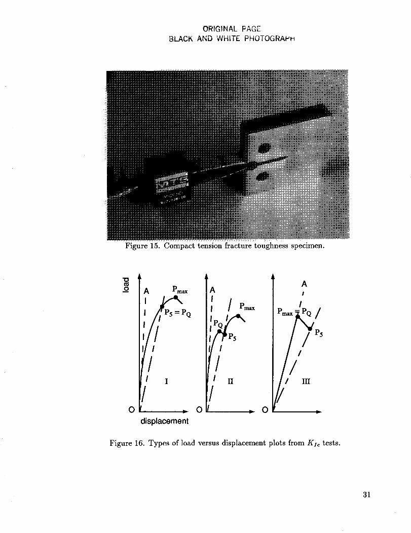
men is loaded to fracture. The crack opening displacement (Figure 15) and specimen
load are recorded during the test. The three types load versus displacement plots
from KI_ tests are shown in Figure 16. Type I is characterized by gradually increas-
ing nonlinearity and Type II is characterized by sudden crack extension and arrest
or "pop-in" followed by nonlinearity. Type III is characterized by almost perfectly
elastic behavior and is uncommon.
A candidate value of fracture toughness, KQ, is calculated using the load PQ
determined as follows:
• The load corresponding to the intersection of a 5 percent secant offset line drawn
from the origin with the load-displacement curve is denoted Ps.
• If the load-displacement plot is Type I, then Pc2 = Ps.
• If the load-displacement plot is Type II, then Pc2 is the highest load preceding
P5 on the load-displacement curve.
• If the load-displacement plot is Type III, then Pc2 = P._a_.
The ratio Pm_,/PQ must be less than 1.1 to ensure that excessive stable crack growth
does not occur during the test. The value of KQ is calculated using the stress intensity
factor equation from section 3.4. If all the previous conditions are met, the test is
valid and KI_ = KQ. [4, 39]
3O
ORIGINAL PAGE
BLACK AND WHITE PHOTOGRAP_
Figure 15. Compact tension fracture toughness specimen.
A
I1_ / I P_ _/PSI/ '
/_ [/! II _ III
0 0 _ 0
displacement
Figure 16. Types of load versus displacement plots from KIc tests.
31
4.3 Plane Stress Fracture Toughness Testing
Values of critical stress intensity factors for thinner plates are denoted simply
as Kc, the plane stress or transitional fracture toughness. The thicknesses used in
actual structures are often much less than the thickness needed for a valid Kic test.
Therefore, a test-verified methodology for determining K_ is of practical interest.
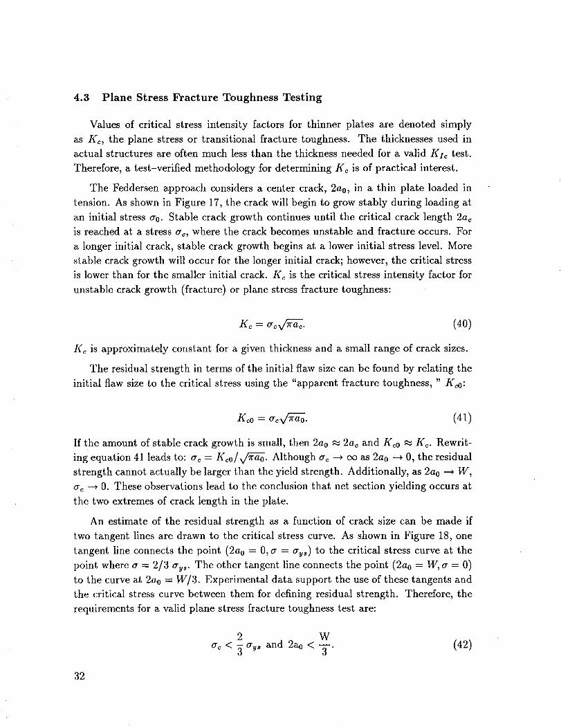
The Feddersen approach considers a center crack, 2a0, in a thin plate loaded in
tension. As shown in Figure 17, the crack will begin to grow stably during loading at
an initial stress a0. Stable crack growth continues until the critical crack length 2a_
is reached at a stress a_, where the crack becomes unstable and fracture occurs. For
a longer initial crack, stable crack growth begins at a lower initial stress level. More
stable crack growth will occur for the longer initial crack; however, the critical stress
is lower than for the smaller initial crack. K_ is the critical stress intensity factor for
unstable crack growth (fracture) or plane stress fracture toughness:
Ko= (40)
Kc is approximately constant for a given thickness and a small range of crack sizes.
The residual strength in terms of the initial flaw size can be found by relating the
initial flaw size to the critical stress using the "apparent fracture toughness, " K_0:
K_0 = a_ _v/-_-_. (41)
If the amount of stable crack growth is small, then 2a0 _ 2ac and Kc0 ,-_ K_. Rewrit-
ing equation 41 leads to: a_ = K_o/_x/"_. Although a_ -_ oo as 2a0 -4 0, the residual
strength cannot actually be larger than the yield strength. Additionally, as 2a0 --_ W,
ac --+ 0. These observations lead to the conclusion that net section yielding occurs at
the two extremes of crack length in the plate.
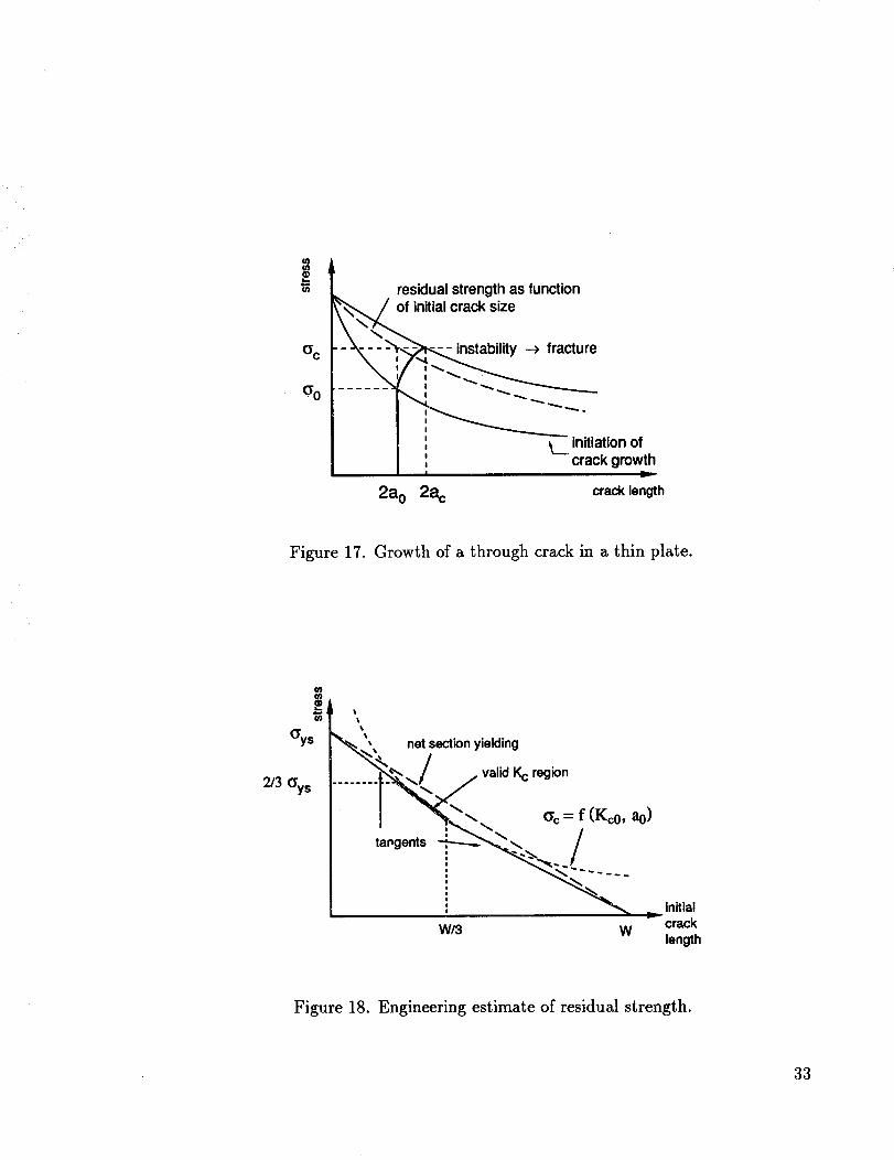
An estimate of the residual strength as a function of crack size can be made if
two tangent lines are drawn to the critical stress curve. As shown in Figure 18, one
tangent line connects the point (2a0 = 0, a = ays) to the critical stress curve at the
point where a = 2/3 ay,. The other tangent line connects the point (2a0 = W, a = 0)
to the curve at 2a0 = W/3. Experimental data support the use of these tangents and
the critical stress curve between them for defining residual strength. Therefore, the
requirements for a valid plane stress fracture toughness test are:
2 W
a_ < _ ay_ and 2a0 < --_-. (42)
32
%
_0
residual strength as function
of initial crack sizebility --> fracture
,' __. initiation of,' crack growthI ID_
2a o 2a c crack length
Figure 17. Growth of a through crack in a thin plate.
2/3 Gys
t t
_,,_, net section yielding
_'%_\ _c = f (K¢0, a0)
tangents _._ /
v
W/3 W
initialcrack
length
Figure 18. Engineering estimate of residual strength.
33
The Kc tests should be conducted on fatigue precracked specimens using the
actual thicknesses and crack lengths of interest. Any stable crack growth during the
test should be recorded, as well as the load and time. The fracture load should be
taken as the maximum load in the test. Unconservative errors in estimating residual
strength will result if the requirements on stress level and crack size are not met. [4]
34
5 SUBCRITICAL CRACK GROWTH
5.1 Fatigue Crack Growth
Fatigue cracks originate at geometric stress concentrations (holes and fillets) and
at manufacturing flaws (tool scratches, impact dents, and pits caused by welding arc
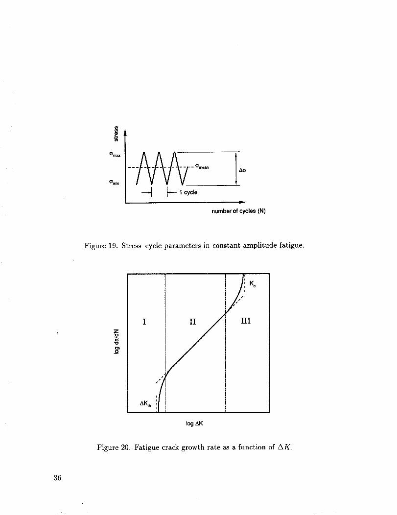
strikes). A fatigue crack can grow under the cyclic loading shown in Figure 19, finally
reaching its critical length and fracturing. The stress range Aa = ama_: - ami,_ can
be related to the stress intensity factor range, AK:
AK = K,,_a_- Kmin,
A K = Aa _ __ v/'_'d - Aa ,,_i , V/'_-a,
AK = _Aa vr_,
(43)
where K.,.. and Kmin are the stress intensity factors associated with the maximum
and minimum stresses in a fatigue cycle and A is the correction factor discussed in
section 3. The growth rate of a fatigue crack is related to AK and the load ratio, R:
groin
n- Km_" (44)
d_ is the crack extension Aa during a smallThe fatigue crack growth rate, 7-_,
number of fatigue cycles AN. Fatigue crack growth rate is a function of the stress
intensity factor range AK and stress ratio R. Data of aa_AK for a given R areaN
usually presented on a log-log plot as shown in Figure 20. The crack growth rate
curve has a sigmoidal shape which divides the curve into three regions. In region I,
a threshold value of AK occurs. Ideally, the crack will not grow if AK drops below
this threshold, s Above AKth, the crack growth rate increases rapidly with increasing
AK. Crack growth rate in this region is influenced by microstructure, mean stress,
and environment. Region II is characterized by a linear log-log relationship between
d___and AK; this region is influenced largely by certain combinations of environment,dN
mean stress, and frequency. Microstructure and thickness have little influence on the
crack growth of region II. In region III, the crack growth rate rises to an infinite
slope caused when K_a_ --+ Kc. Microstructure, mean stress, and thickness are iaige
influences on the crack growth rate in this region. [3]
SASTM has defined the stress intensity factor range threshold AKth as the AK value associated
with d_ = 4 X 10⁻⁹ inches/cycle. [40]
35
{D
(_min
numberof cycles(N)
Figure 19. Stress-cycle parameters in constant amplitude fatigue.
Z
A_h
i/c=I/ II/ I
,/I I
logAK
Figure 20. Fatigue crack growth rate as a function of AK.
36
As previously mentioned, a threshold value, AKth, exists below which significant
crack growth does not occur. Knowledge of AKth has considerable practical ad-
vantage. If either sufficiently small flaws can be ensured by the planned inspection
techniques or if sufficiently small working stresses are maintained such that AK is
less than AKth, then no fatigue crack growth can occur and the crack can never reach
critical length. In some situations it may be desirable to design for nonpropagating
flaws. However, threshold testing is very difficult to perform and the uncertainties
involved in the analysis make design using AK < AKth questionable. The design
problem of using AK < AKth is analogous to the problem of using Aa < Aa_, where
Aa_ is the fatigue endurance limit. Many materials have no true endurance limit and
the stress range corresponding to a life of l0 s cycles is used in place of Aa_. The use
of arbitrary definitions for AKth and Aa_ for an infinite life design should be viewed
with skepticism.
Attempts to describe the crack growth rate curve using empirical formulas have
been widespread. For a fixed load ratio, R, and a wide range of AK values in region
II, the data can usually be represented as a straight line on the log-log plot. The
Paris equation describes crack growth in region II:
da
d--N = C(AK)n' (45)
where C and n are empirical constants determined experimentally for the given ma-
terial. The effects of load frequency, temperature, and operating environment are
empirically contained in the constants C and n. Table 6 contains a list of these con-
stants for different materials. Note that C has the units of in/cycle( ksiv_)" and n
is a dimensionless exponent which can be thought of as the slope of the crack growth
rate curve. Other dimensional units may be used, so care must be taken to maintain
consistent units when peforming fatigue crack growth analysis. For most materials,
the value of n ranges from 2 to 4.
The references listed in Section 4.1 for fracture toughness data also contain fatigue
crack growth data. Special care should be taken if data from literature sources are
used to ensure that the data correspond to the actual environment or are conser-
vative with respect to the actual environment. Most a_7-_-AK curves are generated
using R _ 0 and room temperature. For some materials, da7-_-AK curves have been
generated at several different stress ratio, temperature and environments, and load
frequency. Interpolation of these curves is often necessary and should be performed
by experienced metallurgists and engineers. Guidelines for using literature sources
are discussed in Reference [41].
37
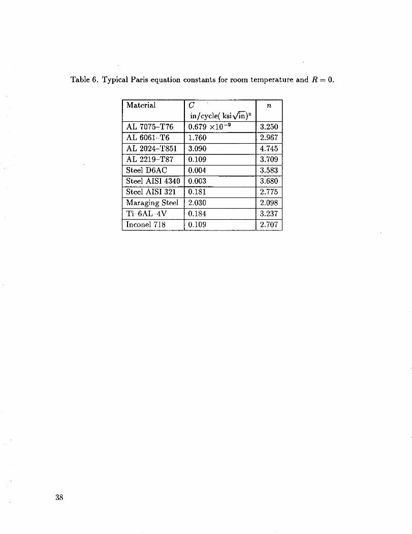
Table 6. Typical Paris equation constantsfor room temperature and R = 0.
Material C
in/cycle( ksi Vq'_) n
AL 7075-T76 0.679 xl0 -9
AL 6061-T6 1.760
AL 2024-T851 3.090
AL 2219-T87 0.109
Steel D6AC 0.004
Steel AISI 4340 0.003
Steel AISI 321 0.181
Maraging Steel 2.030
Ti-6AL-4V 0.184
Inconel 718 0.109
n
3.250
2.967
4.745
3.709
3.583
3.680
2.775
2.098
3.237
2.707
38
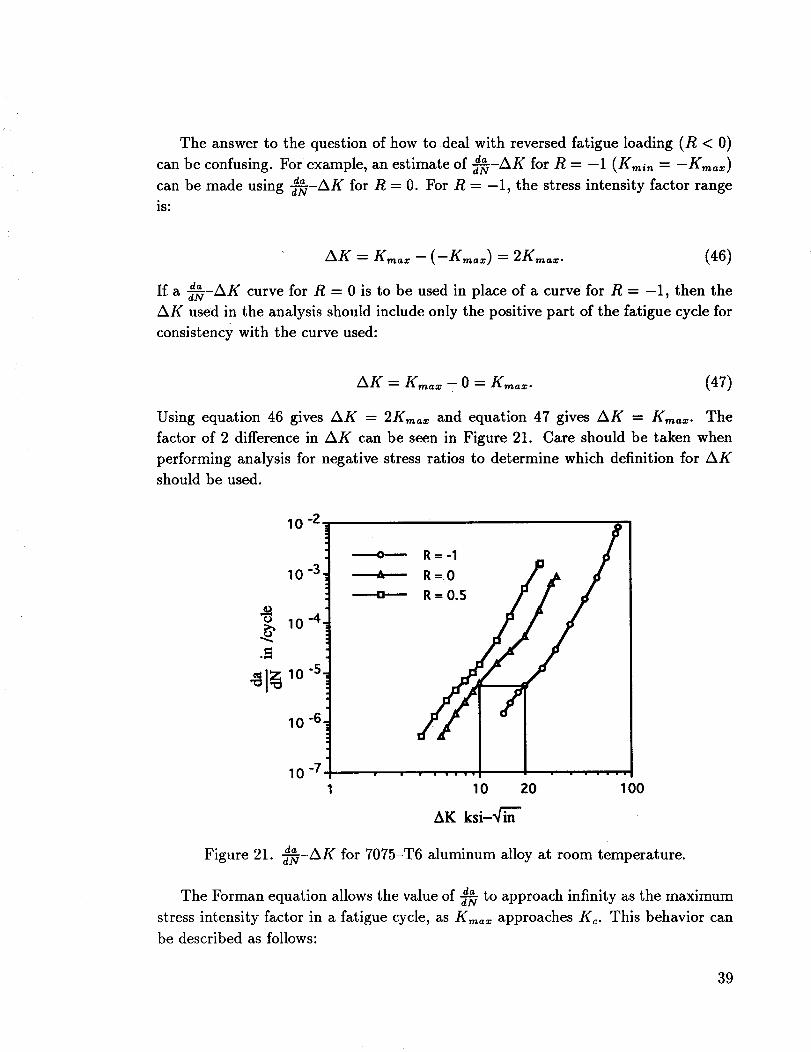
The answer to the question of how to deal with reversed fatigue loading (R < 0)
can be confusing. For example, an estimate of dA-_-AK for R = -1 (K,,.. = -K,,,_)
can be made using dA_-AK for R = 0. For R = -1, the stress intensity factor range
is:
AK = K,,,=_- (-K,,,=x)= 2K,=_. (46)
da
If a -a--_-AK curve for R = 0 is to be used in place of a curve for R = -1, then the
AK used in the analysis should include only the positive part of the fatigue cycle for
consistency with the curve used:
AK = K,_-0 = K,,a_. (47)
Using equation 46 gives AK = 2K,n:: and equation 47 gives AK = K,n::. The
factor of 2 difference in AK can be seen in Figure 21. Care should be taken when
performing analysis for negative stress ratios to determine which definition for AK
should be used.
10 -2
10 -3.
-4,
,t,-q
lo-s
10 -6,
10 -7
---.a---
R - -1
R=O
R--O.S
//10 20
AK ksi-_--m
100
Figure 21. uY-_-AK for 7075-T6 aluminum alloy at room temperature.
The Forman equation allows the value of a,,-_ to approach infinity as the maximum
stress intensity factor in a fatigue cycle, as Kma_ approaches Kc. This behavior can
be described as follows:
39
d-N= (1- R)K - AK"(48)
By taking Kma. into account, the Forman equation describes regions II and III.
The Walker equation accounts for the relatively weak influence of mean stress level
on crack growth rate:
dam_CdN
AK ]" (49)(1
The constants C and n in Paris, Forman, and Walker equations are not generally
interchangeable: Cp_ris _ CFor,_a,_ _ Cw_tk_ and np_is _ nForman _ nwalker.
The hyperbolic sine equation is capable of fitting the entire crack growth rate
curve:
da
log _/N = C1 sinh [C2(log AK -t- C3)] + C4, (50)
where C1 is a material constant, and C2, Ca, and C4 can be written as functions of
temperature, frequency, and stress ratio. This model [42] has been used extensively for
nickel-base superalloys. Many other empirical equations have been used to describe
fatigue crack growth. [3]-[5]
The equation used to express fatigue crack growth rate as a function of AK can be
integrated to determine the number of cycles required for the crack to reach a given
length. For example, the Paris equation (equation 45) can be used to determine the
number of cycles to failure. To perform the integration, AK must be expressed in
terms of the crack length, a. If ai and a/are initial and final crack lengths, N/is the
number of cycles required for the crack to reach a length of a/is:
folvJ ffJ da (51)NI= dN= , C(AK), _.
If the stress spectrum is known, then the final crack size can be determined as
follows:
NI
C(AK)ndN .._ a, + E C(AKj) '_, (52)j=l
where AKj is a function of/kaj.
4O
In the discussionon crack-tip plastic zones,the approach was to determine acorrectionfactor, ry, for the crack length to account for increased compliance due to
the presence of the plastic zone for steady, monotonic loading. For fatigue loading,
the material must accommodate the deformed region, and reversed yielding occurs in
a region smaller than the monotonic plastic zone. The cyclic plastic zone is smaller
than the monotonic zone because the crack extends into this smaller zone of reversed
yielding:
ry,,_onoton_o (53)ry,cyclic -- 4 '
where ry,,_o,_oto,,c is defined in section 2.3. [5]
Even under general monotonic yielding, LEFM may be valid for fatigue crack
growth because crack growth depends on the cyclic variation of strain instead of the
maximum crack-tip strain. If the crack length and remaining ligament are greater
than the cyclic plastic zone size, then using AK as the crack driving force should be
acceptable. Therefore, the limit of applicability of LEFM for cyclic crack growth is
not as restrictive as the limit for monotonic crack growth. [43, 44]
Another important limitation of LEFM fatigue crack growth is the physical size
of the crack. Cracks less than 0.04 in long are referred to as "short cracks," and are
much smaller than the crack sizes normally used in generating fatigue crack growth
rate curves. Similitude between fatigue crack growth rate and stress intensity factor
range is lost because short cracks tend to grow at higher rates than expected from
d_ AK data taken from long cracks.[3, 5]dN
The previous discussions on fatigue crack growth dealt with the use of fatigue
crack growth rates determined from constant amplitude cyclic loading tests. These
crack growth rates are approximately the same as for random cyclic loading tests
if the maximum stress is held constant and the mean stress and stress range vary
randomly. In the case of variable amplitude loading where maximum stress is also
allowed to vary, the sequence or order of loading cycles can have a significant effect
on crack growth rate. The result is that overall crack growth for random load cycles
can be substantially higher than for constant amplitude load cycles.
Fatigue damage and crack growth are dependent on previous cyclic load history.
A significant delay in crack growth can occur after the intermittent application of
high stresses. This delay is called retardation and can be characterized as a period
of reduced crack growth rate following the application of a peak load higher and
in the same direction as the peak loads immediately following. Acceleration can
be characterized as a period of increased crack growth due to the application of
41
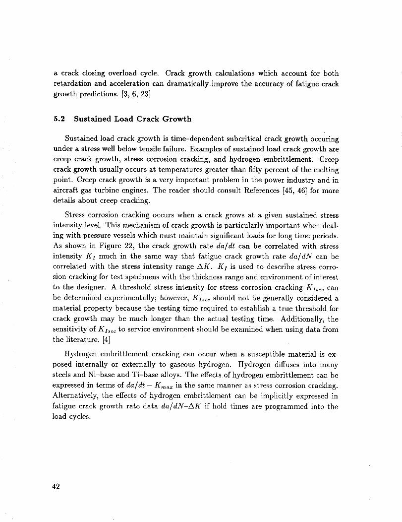
a crack closingoverload cycle. Crack growth calculations which account for bothretardation and accelerationcan dramatically improve the accuracyof fatigue crackgrowth predictions. [3, 6, 23]
5.2 Sustained Load Crack Growth
Sustained load crack growth is time-dependent subcritical crack growth occuring
under a stress well below tensile failure. Examples of sustained load crack growth are
creep crack growth, stress corrosion cracking, and hydrogen embrittlement. Creep
crack growth usually occurs at temperatures greater than fifty percent of the melting
point. Creep crack growth is a very important problem in the power industry and in
aircraft gas turbine engines. The reader should consult References [45, 46] for more
details about creep cracking.
Stress corrosion cracking occurs when a crack grows at a given sustained stress
intensity level. This mechanism of crack growth is particularly important when deal-
ing with pressure vessels which must maintain significant loads for long time periods.
As shown in Figure 22, the crack growth rate da/dt can be correlated with stress
intensity K1 much in the same way that fatigue crack growth rate da/dN can be
correlated with the stress intensity range AK. KI is used to describe stress corro-
sion cracking for test specimens with the thickness range and environment of interest
to the designer. A threshold stress intensity for stress corrosion cracking Kiscc can
be determined experimentally; however, K1sc_ should not be generally considered a
material property because the testing time required to establish a true threshold for
crack growth may be much longer than the actual testing time. Additionally, the
sensitivity of Ki_cc to service environment should be examined when using data from
the literature. [4]
Hydrogen embrittlement cracking can occur when a susceptible material is ex-
posed internally or externally to gaseous hydrogen. Hydrogen diffuses into many
steels and Ni-base and Ti-base alloys. The effects of hydrogen embrittlement can be
expressed in terms of da/dt - Kmax in the same manner as stress corrosion cracking.
Alternatively, the effects of hydrogen embrittlement can be implicitly expressed in
fatigue crack growth rate data da/dN-AK if hold times are programmed into the
load cycles.
42
8
u
0
6 DAMAGE TOLERANCE AND FRACTURE CONTROL
6.1 Philosophy and Basic Assumptions
Damage tolerance and fracture control are both terms used to describe the rigorous
application of engineering, manufacturing, quality assurance, and operations dealing
with the analysis and prevention of crack growth or similar flaw damage leading to
catastrophic event. A catastrophic event is usually defined as a failure event causing
loss of life, injury, or the loss of spacecraft. Fracture control is applied to ensure safety;
fracture control is not mandatory to ensure mission success. However, fracture control
principles should be considered in design even when safety is not an issue.
The general goals of fracture control include the selection of fracture resistant
materials and manufacturing processes, designing access for inspectability, and the
use of multiple load paths or crack stoppers. These goals translate into two specific
objectives: design for safe, stable crack growth (safe-life design) or design for damage
containment due to structural redundancy (fail-safe design). Fracture control requires
the judicious combination of safe-life and fail-safe design. Careful stress analysis,
geometry selection, material selection, surface finish, and workmanship are necessary
prerequisites to effective fracture control.
MSFC-HDBK-1453, "Fracture Control Program Requirements," [51] specifies
that the fracture control status of all spaceflight structures must be determined. If a
structural failure of a part would cause a catastrophic event, then the part is fracture
sensitive. MSFC-HDBK-1453 divides the previously defined fail-safe class into three
subclasses:
• Low mass parts whose release or functional loss will not cause a catastrophic
event
• Contained or restrained parts whose structural failure will not cause a catas-
trophic event
• Structurally redundant (called fail-safe in MSFC-HDBK-1453) parts whose
remaining structure will not cause a catastrophic event.
If a fracture sensitive part cannot be classified as low mass, contained, or fail-safe,
the part is fracture critical. All pressure vessels and high-energy rotating machinery
are classified as fracture critical. A fracture critical part must have a safe-life design;
it must survive 4 complete mission lifetimes in the presence of the largest possible
44
undetected flaw. MSFC-HDBK-1453 specifically uses safe-life to describe metallic or
glass components and damage-tolerant to describe composite components. Fracture
mechanics analyses or tests, flaw screening, and general traceability to ensure proper
implementation and documentation of the fracture control process are required for
fracture critical parts. MSFC-SPEC-522B, "Design Criteria for Controlling Stress
Corrosion Cracking," [47] should be used as a guide in selecting materials to avoid
stress corrosion cracking problems.
There are four basic assumptions for safe-life design:
.
1
Crack-like flaws are inherent in new structures and exist in the most critical
location and orientation.
. Similitude exists between test specimens and actual hardware so that fracture
toughness and fatigue crack growth rate data obtained from test specimens can
be used to predict fatigue crack growth and final crack instability in actual flight
hardware.
0
.
It is assumed that a scatter factor (the scatter factor in MSFC-HDBK-1453
is 4) can be applied to the service life to conservatively account for scatter
in fracture mechanics material properties and uncertainties in analyses due to
using constant amplitude fatigue crack growth data to analyze parts undergoing
variable amplitude loading.
It is assumed that adequate flaw screening (nondestructive inspection or proof
testing) can be reliably performed on fracture critical parts.
The proper way to implement these fracture control requirements is to develop
a fracture control plan. The fracture control plan documents the design, materials,
fabrication, inspection, and operation activities used to prevent catastrophic failures
due to cracks. C.C. Osgood [48] has written ah outline for a fracture control plan of
a high-performance engineering system:
Design
1. Determine stress and strain distributions.
2. Determine flaw tolerance for regions of greatest fracture hazard.
3. Estimate stable crack growth for typical service periods.
4. Recommend safe operating conditions and specify intervals between
inspections.
45
Materials
1. Determineyield and ultimate strengths.
2. Determinefracture parameters:Kc, Krc, Kts_, da/dN.
3. Establish recommended heat treatments.
4. Establish recommended welding methods.
Fabrication
1. Control residual stress, grain growth, and grain direction.
2. Develop or protect strength and fracture properties.
3. Maintain fabrication records.
Inspection
1. Inspect part prior to final fabrication.
2. Inspect fabrication factors such as welding current and speed.
3. Proof test.
4. Estimate largest crack-like defect sizes.
Operation
1. Control stress level and stress fluctuations in service.
2. Protect part from corrosion.
3. Inspect part periodically.
6.2 Flaw-Screening Methods
6.2.1 Nondestructive Inspection
Critical initial flaw sizes are calculated for all likely crack locations in the structure
using fracture mechanics, then nondestructive inspection (NDI) 9 is used to reliably
find flaws at those locations. MSFC-STD-1249, "Standard NDE Guidelines and
Requirements for Fracture Control Programs" [49] requires that the smallest flaw
that NDI can reliably detect must be smaller than critical initial flaw size. Table 7
contains a list of approved initial flaw sizes for several NDI methods. Initial flaws
smaller than those shown in Table 7 may be assumed if a.NDI demonstration verifies
that a 90 percent probability of detection with a 95 percent confidence level exist for
the smaller size.
9Nondestructive inspection (NDI) is also called nondestructive testing (NDT) or nondestructive
evaluation (NDE).
46
A. P. Parker [50]describesthe commonNDI methods:
Eddy current. A small coil induces eddy currents in the metal component. This
reinduces a current in the coil. A change in the inductive "fingerprint" of a
component may indicate a crack or defect.
Dye-penetrant. Suitable for surface cracks only, the method involves the appli-
cation of a liquid penetrant, which is subsequently wiped off the surface before
application of a powdered "developer." Cracklike defects will produce a con-
trasting colored line on the developer.
Magnetic particles. Fluorescent liquid containing iron particles in suspension is
applied to a component. When placed in a strong magneteic field and illumi-
nated with ultraviolet light, disturbances in magnetic field induced by cracks
and cutouts appear as a change in the field pattern. Limited to magnetic ma-
terials.
Radiography. In the case of x-ray or "t-ray radiography, a portable source is
used to irradiate the component, and the absorption assessed from the image on
a sensitive film on the opposite side of the component from the source. Cracks,
which absorb less radiation, appear as dark areas on the film. The method
is sensitive, and may be used to detect internal cracks. However, poor crack
orientation may produce inferior images.
Ultrasonics. A probe emits a high frequency sound wave into the component,
which is reflected by surfaces, including internal cracks. The time taken for
transmission and reflection of a pulse is normally indicated on an oscilloscope.
This may be interpreted as a distance through the component, and hence allow
the crack to be properly located.
The selection of appropriate NDI methods is very important. Accessibility of the
part and operator experience are key factors for successful NDI. Ultrasonics can be
used before machining wrought stock to detect internal flaws. Radiography is less
sensitive than ultrasonics, but it may be easier to apply and can disclose internal
defects that often accompany cracks (inclusions, porosity, and voids). Penetrant
inspection is common for surface flaw detection. Smeared material on machined
surfaces that hides a crack-like flaw should be removed with etchant. If a fine finish
is required, penetrant inspection before final machining would allow etching. More
complicated than penetrant inspection, eddy current inspection should be used if
etching is detrimental or if the surface is coated. Magnetic particle inspection has
limited reliability to detect small flaws. [49]
47
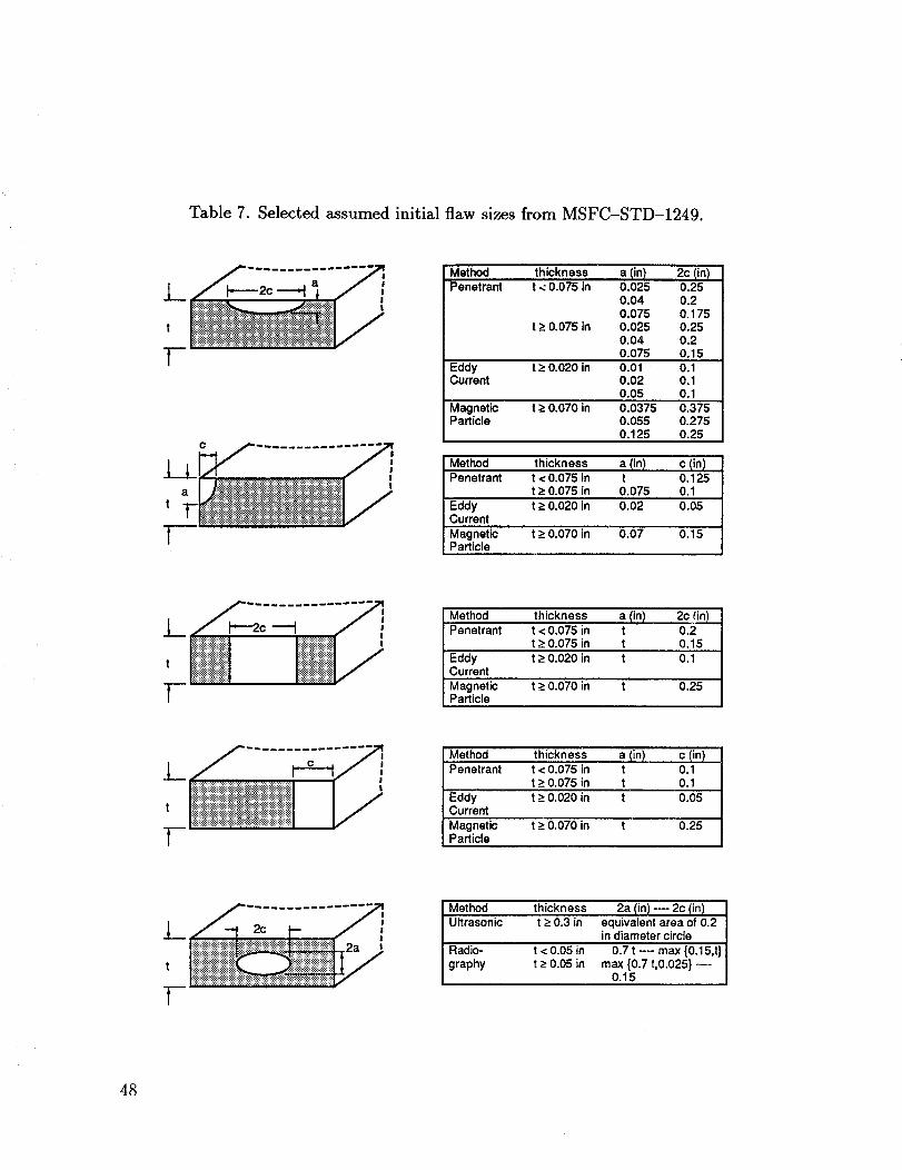
Table 7. Selectedassumedinitial flaw sizesfrom MSFC-STD-1249.
..................... I
t __ __ _':_'_._, '_ _.!!__ __ _!!_i_..'.'_:":.__::.. ,_._J_ _:_....:::::::::::::::::::::::::::::........... _!iii:!i
I
II. . .... I
t =============================================================================================
Method thickness a (in) 2c (in)Penetrant t < 0.075 in 0.025 0.25
0.04 0.20.075 0.175
t >_0.075 in 0.025 0.250.04 0.20.075 O.15
Eddy t > 0.020 in 0.01 0.1Current 0.02 O.1
0.05 0.1
Magnetic t _>0.070 in 0.0375 0.375Particle 0.055 0.275
0.125 0.25
Method thickness a (inI c lin)Penetrant t < 0.075 in t 0.125
t _>0.075 in 0.075 O.1
Eddy t _>0.020 in 0.02 0.05Current
Magnetic t _>0.070 in 0.07 O.15Particle
Method thickness a (in) 2c (in)Penetrant t < 0.075 in t 0.2
t_> 0.075 in t 0.15
I_ IIIIIIIIIIIIII I
I
t iiliiil [Yl
Eddy t > 0.020 in t 0.1Current
Magnetic t _>0.070 in t 0.25Particle
Method thickness a (inI c (in I 1
Penetrant t < 0.075 in t 0.1t _>0.075 in t O.1
Eddy t _>0.020 in t 0.05Current
Magnetic t ->0.070 in t 0.25Particle
Method thickness 2a (in)---2c (in) IUltrasonic t > 0.3 in equivalent area of 0.2 I
in diameter circle IRadio- t <O.05in 0.7 t -- max {0.15,t} I
graphy t_> 0.05 in m_..1{50.7t,0.025}--- I
IIIIiIIiIIIIIIII
I
48
6.2.2 Proof Testing
Proof testing has been extensively used to screen out gross material and man-
ufacturing defects. These defects are eliminated under controlled circumstances to
prevent catastrophic failure during actual service. Proof testing is a useful supple-
ment to conventional NDI when the maximum permissible flaw can escape detection
by NDI, when a structure is too large to make complete NDI feasible, and when the
geometry is too complex to make NDI reliable.
Proof testing is typically performed with a pressure that exceeds the maximum
operating pressure subject to the requirement that the nominal stresses remain below
85 percent of the ultimate strength of the material. Proof testing should be per-
formed in the actual operating environment. However, it is not always possible to do
this because of safety and cost constraints. An environmental correction factor that
accounts for the differences between the material's response in the proof environment
and the material's response in the actual operating environment should be applied.
In cases where the required proof test factor in the actual environment is very large,
it may be desirable to proof test at lower temperatures where the material's fracture
toughness is reduced. The resulting proof test factor will also be reduced.
For a proof test to be effective, the structure must be made of a material that
acts in a brittle manner when the service load and environment is applied. For a
brittle material undergoing proof testing, the existing cracks below the critical flaw
size do not grow to failure. In this regard, the proof test can be seen as a destructive
inspection because only existing cracks equal to or larger than the critical flaw size
will grow to failure. It is assumed that no crack survives that is larger than the critical
flaw size determined for the proof cycle. Therefore, a margin of life is obtained because
the service load is smaller than the proof load. This margin of life is the number of
cycles it takes to grow the largest flaw size that could survive proof to the critical
flaw size at the service conditions. The reader should consult Reference [52] for more
details.
49
7 MISCELLANEOUS TOPICS
7.1 Relationship Between Kz and kt
The dimensionless stress concentration factor, kt, accounts for the increase in
nominal stress due to geometry: a,,,_= = kt a. Both notch length and notch root
radius influence kt. The stress intensity factor, Kz, accounts for both geometric
variables (crack length explicitly and crack-tip radius implicitly because the radius is
assumed to be very sharp) and the stress level. Kz provides the complete stress and
displacement field near the crack tip, whereas, kt provides the useless result kt = cx_
at the crack tip regardless of notch size and shape and stress level.
It is often advantageous to relate the stress concentration factor solution of a
notch to the stress intensity factor solution of a crack because of the large number
of existing stress concentration solutions for notches. [16] Recall that the stress ayy
directly ahead of the crack is:
gi
auy - 2Vz_-_. (54)
If this equation is used to approximate the stress near a notch of root radius p and
root stress O'max, then
Kz= Co',n,_v/'fi, (55)
as p _ 0. For the notch solution of an elliptical hole under uniform tension:
(56)
where a is the remote stress, a is the semimajor axis, and p is the semiminor axis. As
the semiminor axis becomes small, it becomes the root radius of the crack tip, while
the semimajor axis becomes the crack length. In equation 56, the stress concentration
factor kt is:
kt = 1 + 2_/_. (57)
Substituting equation 56 into equation 55 and taking the limit as p _ 0 yields:
5O
Comparingthe aboveequation to K1 = av/'_'a, the constant C = x/_/2. Therefore,
KI can be computed from a corresponding notch solution:
K, = _im [--_-am_=Vzfi ]. (59)
This equation can be very useful in estimating K1 for many notch problems. [5, 9]
7.2 Leak Before Burst
The condition of leak before burst (LBB) occurs when initial flaws in a pressure
vessel safely grow through the pressure wall without causing immediate catastrophic
failure. The transition of surface cracks into through cracks is the basic concern of
LBB. The LBB condition cannot be met for arbitrarily large flaw sizes because for a
given pressure, there is always a flaw size large enough to cause the pressure vessel
to burst. A reasonable approach to leak before burst of a thin-wall pressure vessel is
to consider the size of the assumed initial flaw from the NDI method selected for the
pressure vessel. M.F. Kanninen [46] developed the following approach.
Suppose the crack length is long compared to the crack depth as shown in Fig-
ure 23. This assumption will be conservative for all crack aspect ratios. The initiation
of unstable crack growth in the radial direction (through the thickness) occurs when:
K,c = 1.12 pR _ ec (60)-7-
At crack breakthrough, the through crack will likely have a length equal to the length
of the original surface flaw. The critical condition for unstable crack growth is:
Kc pR 1+1.61--. (61)t Rt
In equation 60, Kic, the plane strain fracture toughness, is used for the failure con-
dition because the surface crack can be highly constrained. In equation 61, Kc, the
plane stress fracture toughness, is used for the failure condition because the through
crack for a thin wall undergoes plane stress constraint.
51
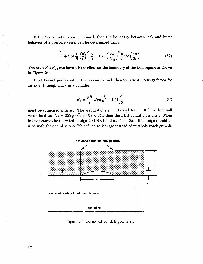
If the two equations are combined, then the boundary between leak and burst
behavior of a pressure vessel can be determined using:
[1+1.61 _=1.25\Kic) -tsec _- .
The ratio Kc/K1c can have a large effect on the boundary of the leak regime as shown
in Figure 24.
If NDI is not performed on the pressure vessel, then the stress intensity factor for
an axial through crack in a cylinder:
c2KI = s/r_ 1 + 1.61_-_ (63)
must be compared with Kc. The assumptions 2c = 10t and R/t = 10 for a thin-wall
vessel lead to: K1 = 255 p V_. If K1 < K_, then the LBB condition is met. When
leakage cannot be tolerated, design for LBB is not sensible. Safe--life design should be
used with the end of service life defined as leakage instead of unstable crack growth.
assumed border of through crack
j ",.::::::::::::::::::::::::::::::::::::::::::::::::::::::::::::::::::::::::::::::::::::::::::::::::::::::::::::::::::::::::::::::::::::::::===:==::=:===:==:====i=====:===:=::::::::::::::::::::::::::::::::::::::::::::::::::::::::::::::::::::::::::::::::::::::==::====i:==:iiiii:=::==:::::::::::::::::::::iiiiiiiiiiiiiiiiiiiiiiiiiiiiiiiii_!ii!_!!!_!i!i!!_!!_i!iiiiiiiiiiiiiiiiiiii!ii_i_i_!!::ii::i::ii::!::!:/:i::i::::::::::::::::::::::::::::::::::::::::::::::::::::::::::::::::::::::::::::::::i!::_ilii!:!:!i_i_:!ii:_:!:i:!::_i_!i!i iiiiiiiiiiii i i i iiiiiiiii ii iiii!i!!!ii !!! !! !ii ill !i! i!iiiiiiiiiiiiiiiiiiiiiiiiii!! ii!iii Ei_i_!iiiiiiiii!!!ii i !i_iiiiiiiiiiiiiiiiiiiiiiiiii;iiiiiiiiiiiiiiiii_i!i:i!iii_i:i!:::::::::::::::::!:;:!!!!_i iii!iiiii!!!ii!!!iiiiiiiiiiiiiiiiiiiiiii_iiii_i_i_!!i!!i!iiiiiii!iiiiiiiiiiiiii_E_!i_ji_!!!_!!i!iiiiiiii!iiiiiiiiiiiiiiiiiiiiiiiiiiiii;i;iiiii!iiiii_ i_iiiii_i;i:i:iii!i_ii!iiii_iiiiiiiiii;;i;iiiiiiii;;;;i;iiiiii;;iiii_!i!ii!!iii!iiiiiii;iii;;;;iiiiiii_;iii_ii!_i!_iiii;;i!_iiii;iiiiiii;iiiiiiiiiiiiiiiiiiiiii;;;;i;;i;;iii_i;i!iii_i;;i;i;;;::::::::::::::::::::::::::::::::::::::::::::::::::::::::::::::::::::::::::::::::::::::::::::::::::::::::::::::::::::::::::::::::::::::::::::::::::::::::::::::::::::::::::::::::::::::::::::::::::::::::::::::::::::::::::::::::::::::::::::::::::::::::::::::::::::::::::::::::::::i::::::::_iliil i ii[_!!i_iiiiiiii i iiiiiiiiiiiiiiiiiiii_i i i i _ i iE i !; _!__i__i i i i i ii i i i i i i i i i i i ii i i i i_ii i i i i iii !_ii i;Ei!_i_i_i_i_!_!!_:_:!:i:i:i:i:i:i:i:i:i:i:i:]:i:i:i:i:i:i:i:i:i:i:i:;:]:i:i:i:i:i:i:i:_!_!iiE!_!_!i_i!iiiiiiiiiiiiiii[iiiiii!iiiiii_i!!i_!i_i_i!_!iiiiiiiiiiiiiiiiiiii!iiiiii!iiiii!_i!_i_iii_i_!_i!i!_iiiiiiii!iiiiiiiiiiiiiiiiiiiiiiiiiiiiiii!iii iiiii;iiiiiiiiiii
_i N N ;-:_:!_i_!il/! _i N N i# i_ _i_! _! N N ?# i_ :7_:'_'':.........................:"'::_:_i_i _? _!_ N _ !_, :_:_: ,_: _: N _ :_ :?.!._:_: ,_,
!iii [iiiii!iii!iiiii i iTiiiiiiiii i iiiiiiiiii i [ii_[_iii i:i::::':"" ':::::i:ii iii _i ii_ i__!ii!iiiii!i!iiiiiiiiiiiii?i?i?i?iiiiiiiiiiiiiiiiiiliii[iiiiiiiiiiiii
_:::::::::::
.....................................................................................i:i........... _:=:i=i:i=i==:=,:i:i...............................i....
I" 2c -I la
assumed border of part through crack
centerline
Figure 23. Conservative LBB geometry.
52
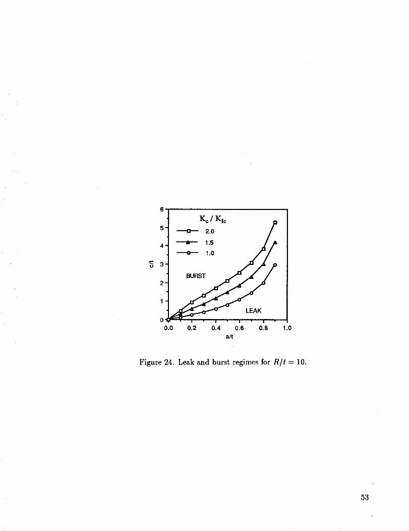
Z_l KI_ P5-
2.0 /I--,- Is i:4-
_1o //:2
I
0 _ LEAKI " I " I " l •
0.0 0.2 0.4 0.6 0.8
a/t
1.0
Figure 24. Leak and burst regimes for R/t = 10.
53
8 EXAMPLE PROBLEMS AND PRACTICE SET
8.1 Example Problems
8.1.1 Stress Intensity Factor Calculation
A 6061-T6 aluminum alloy plate is 10.0-in wide and 0.25-in thick. The plate's
fracture toughness Kc is 27 ksiv_ and the operating load P is 90,000 lb. Is the plate
safe in the presence of a 0.5-in edge crack? If not, what is the critical load?
Assume that the stress due to P is uniformly distributed across the plate:
P 90,000 lba - - = 36.0 ksi.
a (0.25 in)(lO.O in)
The stress intensity factor is given by equation 14:
Ki = Aax/_.
For _ = 0.05 and )_ = 1.1343 (section 3.4, case 2), KI becomes:
K, = 1.1343(36 ksi)_/_-(0.5 in) = 51 ksiv_m.
Therefore, the plate is unsafe with a 0.5-in crack because KI > Kc.
To calculate the critical load for the 0.5-in crack, let K, = Kc and a = a_, then
calculate the correction factor )_ and solve equation 14 for the critical stress:
Substituting the previously determined quantities into the above equation:
27 ksiv_- 19 ksi.
a_ = 1.1343-_r(0.5_/ in)
54
The critical load is:
Pc = acA = (19.0 ksi)(0.25 in)(10 in) = 47,500 lb.
Therefore, the plate fails at a much lower load than the operating load. To calculate
the critical flaw size at the operating load, use equation 14 with a = ac and K, = Kc:
1 (Kc'_ 2a c = --
7r kAaJ '
where )_ is a function of ac. The critical crack length was iteratively determined to
be 0.14 in, well below the planned 0.5 in. The following options could be considered
in the design change:
• Use a material with a higher Kc value.
• Lower the operating stress.
• Change the component configuration.
• Improve the inspection by increasing the accessibility of the part, allowing the
use of a more sensitive technique, or decreasing the period between inspection.
8.1.2 Factor of Safety for Critical Stress
A high strength steel alloy plate 10-in wide and 1.875-in thick may contain surface
cracks. The planned NDI technique can detect a surface crack 0.375-in deep and 0.75-
in long. The material's fracture toughness is 95 ksix/_. If the allowable stress for the
material is 60 ksi, determine the factor of safety for the plate.
Table 1 can be used to determine the correction factor At for a semi-elliptical
a = 0.2, At = 1.174 at ¢ = 0 and )_t = 1.049 at ¢ = 7r/2.surface crack. For _ = 1 and 7
Solving the stress intensity factor equation for the critical stress gives:
KC
where )_tot = (_t)%,)/(b. The finite width correction (calculated from equation 36) is
)_ = 1.0007. For a/c_ 1, the elliptical integral is (I) = 7r/2. Combining these values
55
gives Atot = 0.7479 at ¢ = 0 and Atot = 0.6683 at ¢ = _r/2. Using the largest total
correction factor will give the lowest value for critical stress:
The factor of safety is:
95 ksiv_ac = - 117 ksi. (65)
0.7479¢_r(0.375 in)
F.S. - ac _ 117 ksia 60 ksi = 1.95. (66)
8.1.3 Crack Growth in a Plate
A large, wide plate (use A = 1) contains a 0.20-in through crack. The plate is
subjected to a cyclic operating stress that varies between 5 and 25 ksi. The fatigue
crack growth rate can be expressed using Equation 45 with C = 5 x 10 -l° and n = 4.0
(AK is expressed in ksiv_, and da/dN in inches/cycle). Kc is 60.0ksiv_ and AKth
is 10.0ksiv/_. (a) Determine the number of cycles required for the crack to grow from
an initial size, 2ai, of 0.20 in to a length of 0.5 in. To determine the number of cycles,
equation 45 must be integrated:
da
dN - C(AK)'_ = C(Aax/_-_)n"
Solving for the number of cycles:
N f = rjoNJ dN
Substituting values,
1 ffl da,
1 [o.25 daNI = 5 × 10⁻¹°(20V/-_) 4"° .,0.1 (v/-ff) 4"°"
Solving the integration yields:
Nf =
Nf =
1 [(0.25)_1. 0 __ (0.1)_1.0 ]5 X I0-10(20V/_) 4"0
7,600 cycles.
56
(b) Determine the number of cycles for the crack to grow from an initial length
of 0.20 in to failure. Failure will occur when the crack reaches the critical length for
the maximum stress of 25 ksi. To determine the critical crack length at this stress,
let KI = Kc:
Solving for ac yields:
Kc = O'rnax_.
(6@= -- 1.83 in.
a_- _rtr_._ 7r(25) 2
To determine the number of cycles it takes for the crack to grow from its initial half-
length, ai = 0.1 in, to its critical half-length, a_ = 1.83 in, let a! = a_ and N! = N_
in the equation for Nf in part (b),
_oN,. 1 Jfa"" daNc = dN - C(Ao'v_)" _ (v/_),,"
Substituting values and integrating yields:
if
NI=
1 [(1.83)_1. 0 _ (0.1)_L0 ]5 × lO-lO(20vf_) 4"0
11,970 cycles.
A total of 11,970 cycles are required for the crack to grow from a half-length of
0.1 in to failure. Growing the crack to 0.25 in required 7,600 cycles, and only 4,371
additional cycles were required to grow the crack from a = 0.25 in to its critical value
of a_ = 1.83in. As the crack grows longer, the stress intensity factor increases causing
the crack growth rate to increase. Figure 25 is a plot of the number of cycles required
to grow the crack to various lengths.
In this example, the correction factor A, in the expression for the stress intensity
factor was unity. In general, the correction factor depends on the crack length and
geometry making the integration indicated in equation 51 more complicated than this
example. In many problems, it is possible to treat A as a constant for a small interval
57
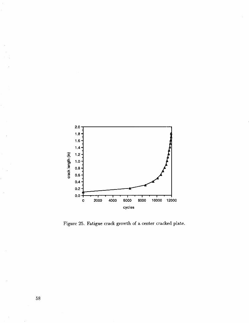
O)¢.-
_e
¢.)
(9
2.0
1.8
1.6
1.4 _
1.2 _
1.0 _
0.8'
0.6'
0.4'
0.2-
0.0
0I I I I I
2000 4000 6000 8000 10000 12000
cycles
Figure 25. Fatigue crack growth of a center cracked plate.
58
of crack extension (Aa ,_ 0.05 in for example). Then a revised value of _ can be used
for the next interval of crack growth. This process can be continued, assuming $ is a
constant for each interval of growth, until the required crack length is reached.
(c) If the plate is to be designed for no crack growth, what is the crack size that
must be screened using NDI? In this case,
=
must be solved for a = ata by letting AK = AKth:
(67)
1 (AKth'_2 (68)ath _-- --7r \ _Aa ]
For a wide plate, the correction factor )t is unity and the threshold crack size is:
1 (10_ 2ath = -- = 0.08 in (69)
Therefore, NDI must reliably detect cracks as small as 0.08 in to ensure no crack
growth in the plate.
8.1.4 Flaw-screening Proof Test Factor
A 10-in wide, I-in thick plate made of 2219-T87 aluminum alloy is cyclically
loaded with a tensile stress ranging between 0 to 15 ksi. The plate is part of a
structure that must withstand 10,000 cycles of operation. Assuming that the most
likely existing crack is a through crack in the center of the plate, determine the proof
test factor necessary to ensure that the plate will withstand 40,000 cycles (10,000
cycles × scatter factor of 4).
For 2219-T87 at room temperature, the yield strength is cru8 = 66 ksi and the
fracture toughness is Klc = 35ksiv/_. The Paris equation constants are C = 0.109 x
10-gin./(ksiv_) n and n -- 3.709. Because the fracture toughness and number of
cycles to failure are known, it is possible to iteratively determine the maximum initial
crack size by guessing an initial flaw size and then comparing the cycles to failure
with 40,000 cycles. A guess of ai = 0.5 in yielded 57,809 cycles to failure, implying
that the desired initial flaw size is larger. Guessing a larger size, ai = 0.75 in, gives
29,267 cycles to failure. Therefore, the desired initial flaw size is bounded between
0.5 and 0.75 in. A final guess, ai = 0.6 in, yielded 43,672 cycles to failure. This 0.6-in
59
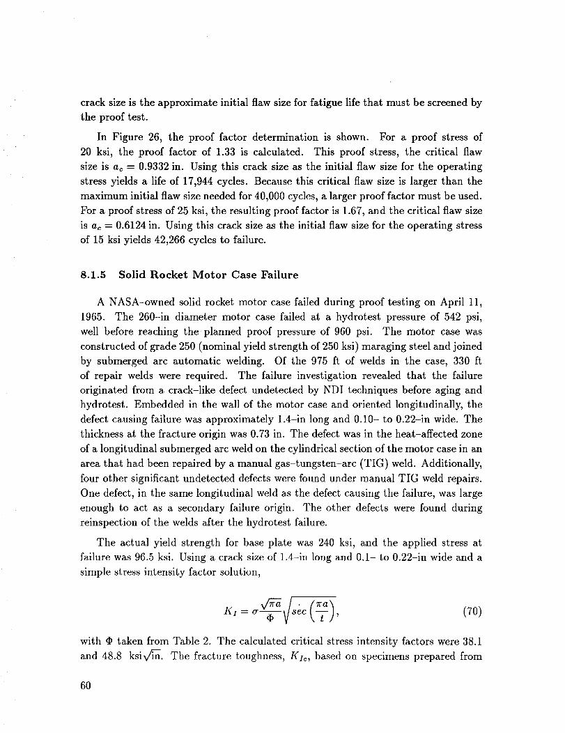
cracksizeis the approximate initial flaw sizefor fatigue life that must be screenedbythe proof test.
In Figure 26, the proof factor determination is shown. For a proof stress of20 ksi, the proof factor of 1.33 is calculated. This proof stress, the critical flawsizeis a_ = 0.9332 in. Using this crack size as the initial flaw size for the operating
stress yields a life of 17,944 cycles. Because this critical flaw size is larger than the
maximum initial flaw size needed for 40,000 cycles, a larger proof factor must be used.
For a proof stress of 25 ksi, the resulting proof factor is 1.67, and the critical flaw size
is a_ = 0.6124 in. Using this crack size as the initial flaw size for the operating stress
of 15 ksi yields 42,266 cycles to failure.
8.1.5 Solid Rocket Motor Case Failure
A NASA-owned solid rocket motor case failed during proof testing on April 11,
1965. The 260-in diameter motor case failed at a hydrotest pressure of 542 psi,
well before reaching the planned proof pressure of 960 psi. The motor case was
constructed of grade 250 (nominal yield strength of 250 ksi) maraging steel and joined
by submerged arc automatic welding. Of the 975 ft of welds in the case, 330 ft
of repair welds were required. The failure investigation revealed that the failure
originated from a crack-like defect undetected by NDI techniques before aging and
hydrotest. Embedded in the wall of the motor case and oriented longitudinally, the
defect causing failure was approximately 1.4-in long and 0.10- to 0.22-in wide. The
thickness at the fracture origin was 0.73 in. The defect was in the heat-affected zone
of a longitudinal submerged arc weld on the cylindrical section of the motor case in an
area that had been repaired by a manual gas-tungsten-arc (TIG) weld. Additionally,
four other significant undetected defects were found under manual TIG weld repairs.
One defect, in the same longitudinal weld as the defect causing the failure, was large
enough to act as a secondary failure origin. The other defects were found during
reinspection of the welds after the hydrotest failure.
The actual yield strength for base plate was 240 ksi, and the applied stress at
failure was 96.5 ksi. Using a crack size of 1.4-in long and 0.1- to 0.22-in wide and a
simple stress intensity factor solution,
with • taken from Table 2. The calculated critical stress intensity factors were 38.1
and 48.8 ksiv_. The fracture toughness, Kz_, based on specimens prepared from
6O
1.6
- --_. ....
,.,,.,t/)i'710.8 I
1 •0.6
0.4_0 10000 20000 30000 40000 50000 60000
N
(a)
_ 20ksi /
i 40_ K _ 25ksi /
•I Iff 25 I20 I
15
lO ;:(d '0.00 0.25 0.50 0.75 1.00 1.25 1.50 1.75 2.00
a (in)
(b)
Figure 26. Determination of proof factor for a center cracked plate.
61
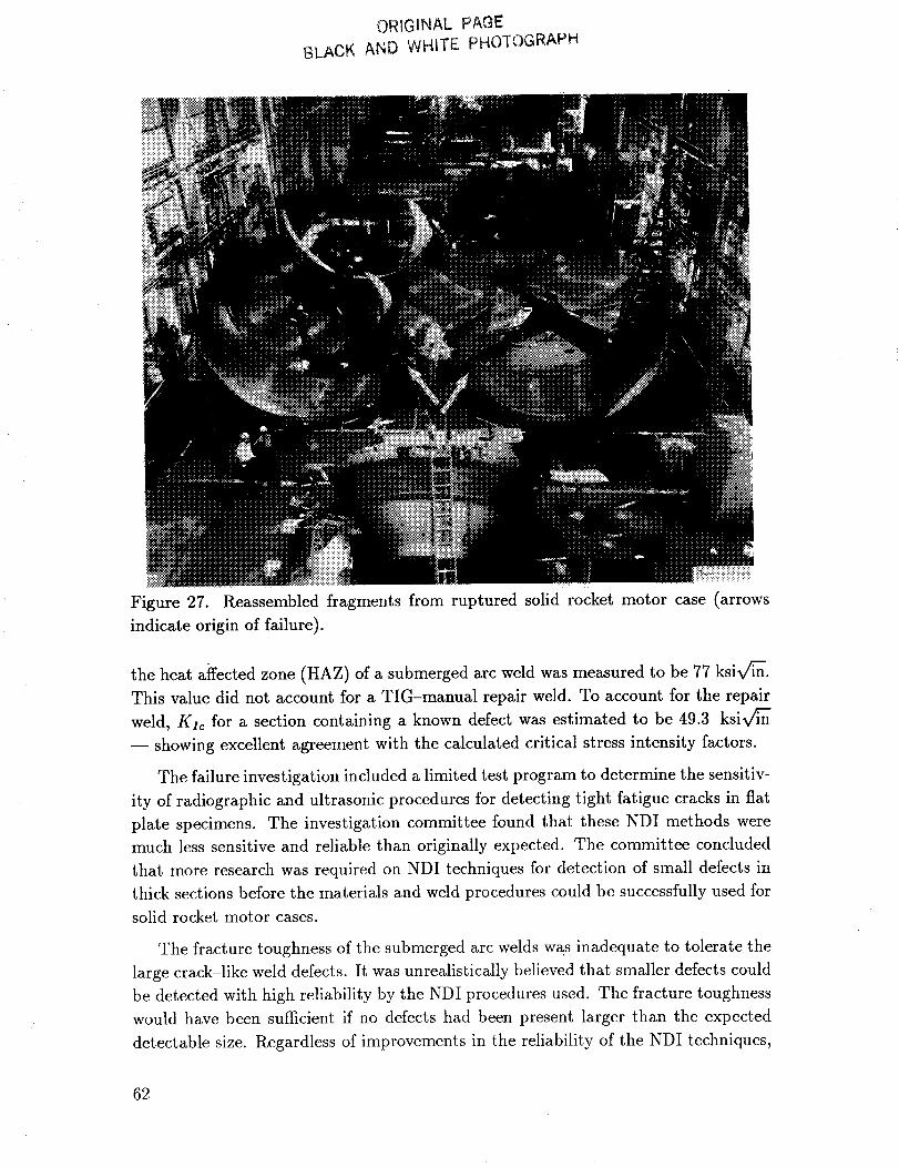
ORIGINAL F_AGE
BLACK AND WHITE PHOTOGRAPH
Figure 27. Reassembled fragments from ruptured solid rocket motor case (arrows
indicate origin of failure).
the heat affected zone (HAZ) of a submerged arc weld was measured to be 77 ksix/_.
This value did not account for a TIG-manual repair weld. To account for the repair
weld, Kzo for a section containing a known defect was estimated to be 49.3 ksiv_
-- showing excellent agreement with the calculated critical stress intensity factors.
The failure investigation included a limited test program to determine the sensitiv-
ity of radiographic and ultrasonic procedures for detecting tight fatigue cracks in flat
plate specimens. The investigation committee found that these NDI methods were
much less sensitive and reliable than originally expected. The committee concluded
that more research was required on NDI techniques for detection of small defects in
thick sections before the materials and weld procedures could be successfully used for
solid rocket motor cases.
The fracture toughness of the submerged arc welds was inadequate to tolerate the
large crack-like weld defects. It was unrealistically believed that smaller defects could
be detected with high reliability by the NDI procedures used. The fracture toughness
would have been sufficient if no defects had been present larger than the expected
detectable size. Regardless of improvements in the reliability of the NDI techniques,
62
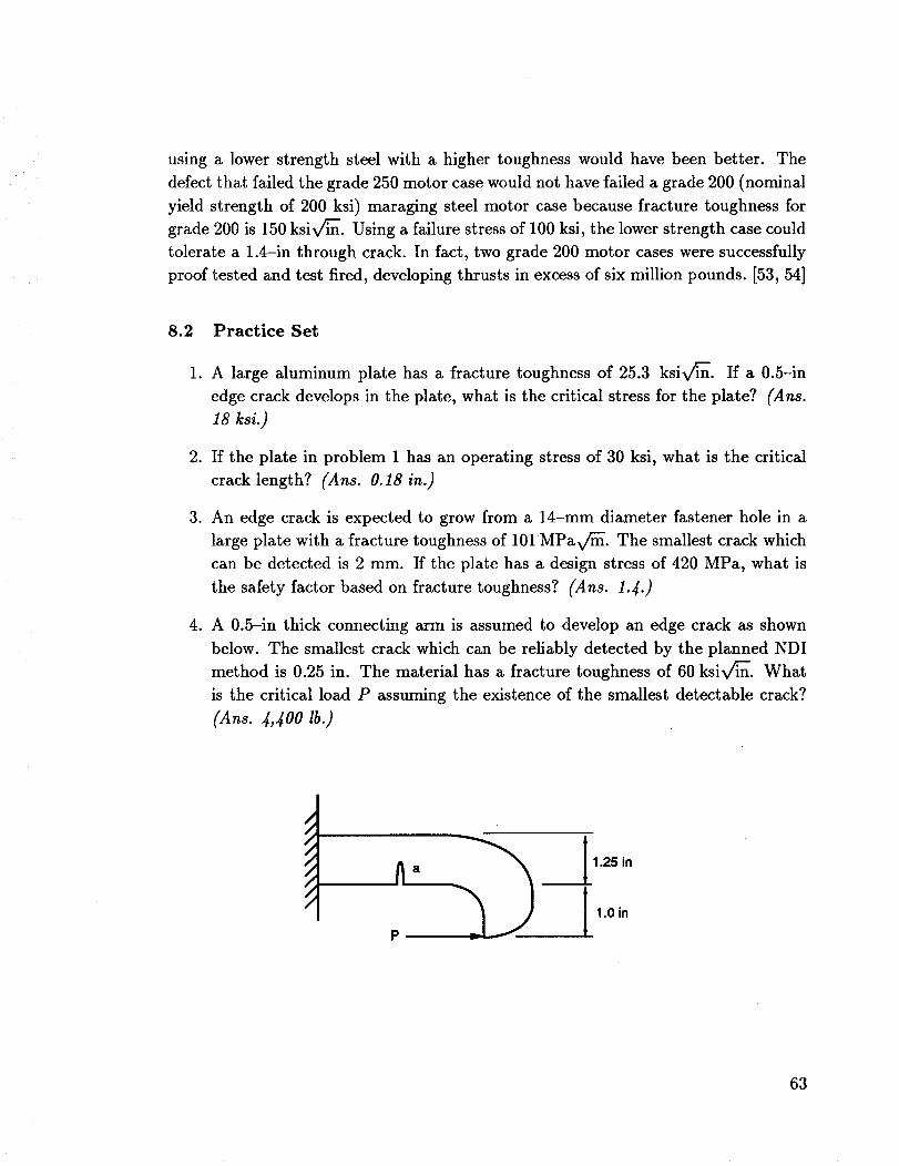
using a lower strength steel with a higher toughnesswould have beenbetter. Thedefectthat failed the grade250motor casewouldnot havefailed agrade200(nominalyield strength of 200 ksi) maraging steel motor casebecausefracture toughnessforgrade200is 150ksiv/_. Usinga failure stressof 100ksi, the lowerstrength casecouldtolerate a 1.4-in through crack. In fact, two grade200 motor casesweresuccessfullyproof testedand test fired, developingthrusts in excessof six million pounds. [53,54]
.
,
.
Practice Set
A large aluminum plate has a fracture toughness of 25.3 ksiv_. If a 0.5-in
edge crack develops in the plate, what is the critical stress for the plate? (Arts.
18 ksi.)
If the plate in problem 1 has an operating stress of 30 ksi, what is the critical
crack length? (Arts. 0.18 in.)
An edge crack is expected to grow from a 14-mm diameter fastener hole in a
large plate with a fracture toughness of 101 MPav/m. The smallest crack which
can be detected is 2 mm. If the plate has a design stress of 420 MPa, what is
the safety factor based on fracture toughness? (Ans. 1.4.)
A 0.5-in thick connecting arm is assumed to develop an edge crack as shown
below. The smallest crack which can be reliably detected by the planned NDI
method is 0.25 in. The material has a fracture toughness of 60 ksiv/_. What
is the critical load P assuming the existence of the smallest detectable crack?
(Ans. 4,400 lb.)
__tl.25 inP [ 1.0 in
63
.
.
.
.
.
10.
A cylindrical pressure tank is assumed to develop a 20-mm axial crack through
the thickness. The tank has a liner to prevent leakage at the crack. The diameter
of the tank is 800 mm and the wall thickness is 5 mm. If the fracture toughness
of the tank material is 40 MPax/_ , what is the maximum internal pressure the
tank can withstand? (Ans. 2.9 MPa.)
A total error of 10 percent exists in the stress analysis and stress intensity
_a is roughlyfactor analysis of a component. If the fatigue crack growth rate
proportional to (AK) 4, estimate the error in the calculated crack growth rate
of the component. (Arts. 45 percent.)
During a proof test, a large cylindrical pressure vessel prematurely failed at an
internal pressure of 5.29 MPa. Inspection of the fracture surfaces revealed an
embedded crack in an axially-oriented weld seam 41 mm long and 4.1 mm deep.
The inside diameter of the pressure vessel was 635 cm and the wall thickness
was 24 mm. If the fracture toughness of the material was 55.5 MPav_ , was the
undetected crack large enough to cause faildre? (Ans. Yes, the critical stress
was 460 MPa and the proof stress was over 700 MPa.)
A cylindrical pressure vessel has a wall thickness of 22 mm and an inside diam-
eter of 538 cm. The smallest crack that can be reliably detected using NDI has
a length of 8 mm and a depth of 4 mm. The material's toughness is 66 MPax/-_
and the internal operating pressure is 4.8 MPa. If the crack is oriented axially,
what is the factor of safety against brittle fracture? (Ans. 1.4.)
A large plate is being designed for the presence of an edge crack. The plate is
subjected to an alternating load that varies sinusoidally from a minimum stess
of 10 ksi to a maximum stress of a,,a_. If the initial crack is 0.125-in long and
the stress intensity threshold is 8 ksix/_, what is the allowable value of area,
for a nonpropagating crack? (Ans. 21 ksi.)
The plate in problem 9 has a toughness of 32 ksiv_. The Paris equation
coefficients are C = 1.5 x 10 -11 and n = 3.1. If the plate is to be designed for
sinusoidally varying load having a minimum stress of 10 ksi and a maximum
stress of 25 ksi, how many load cycles will the plate withstand before the crack
grows from its initial length of 0.125 in to failure? 'Ans. 5,000,000 cycles.)
64
REFERENCES
[1]Forman, R.G., Shivakumar, V., Newman, J.C., Jr., Piotrowski, S.M., and
Williams, L.C.: "Development of the NASA/FLAGRO Computer Program."
Fracture Mechanics: 18th Symposium, ASTM STP 945, pp. 781-803
Philadelphia: 1988.
[2] Harris, D.O., Eason, E.D., Thomas, J.M., Bianca, C.J., and Salter, L.D.:
"NASCRAC -- A Computer Code for Fracture Mechanics Analysis of Crack
Growth." AIAA-87-0847-CP, AIAA/ASME/ASCE/AHS 28th Structures,
Structural Dynamics and Materials Conference, pp. 662-667, Monterey, CA,
April 6-8, 1987.
[3] Broek, D.: "Elementary Engineering Fracture Mechanics." Martinus Nijhoff,
Dordrecht, The Netherlands, 1987.
[4] Ewalds, H.L., and Wanhill, R.J.H.: "Fracture Mechanics." Edward Arnold,
Baltimore, 1986.
[5] Anderson, T.L.: "Fracture Mechanics: Fundamentals and Applications." CRC
Press, Boston, 1991.
[6] Collins, J.A.: "Failure of Materials in Mechanical Design: Analysis, Prediction,
Prevention." Wiley-Interscience, New York, 1981.
[7] Bannantine, J.A., Comer, J.J., and Handrock, J.L.: "Fundamentals of Metal
Fatigue Analysis." Prentice Hall, Englewood Cliffs, N J, 1990.
[8] Wulpi, D.J.: "Understanding How Components Fail." American Society for
Metals, Metals Park, OH, 1985.
[9]Inglis, C.E.: "Stresses in Plate Due to the Presence of Cracks and Sharp
Corners." Transactions of the Institution of Naval Architects, Series A, vol. 55,
pp. 219-230, London, 1913.
[10] Griffith, A.A.: "The Phenomena of Rupture and Flow in Solids." Philosophical
Transactions of the Royal Society, Series A, vol. 221, pp. 163-198, London,
1920.
65
[11]
[12]
[13]
[14]
[15]
[16]
[17]
[18]
[19]
[2o]
[21]
[22]
Irwin, G.R.: "Fracture Dynamics." Fracturing of Metals, Cleveland, American
Society for Metals, 1948.
Orowan, E.: "Fracture and Strength of Solids." Report of Progess in Physics,
vol. 12, 1949.
Irwin, G.R.: "Analysis of Stresses and Strains Near the End of a Crack
Tranversing a Plate." Journal of Applied Mechanics, vol. 24, pp. 361-364,
September 1957.
Williams, M.L.: "On the Stress Distribution at the Base of a Stationary
Crack." Journal of Applied Mechanics, vol. 24, pp. 109-114, March 1957.
Paris, P.C., Gomez, R.E., and Anderson, W.E: "A Rational Analytic Theory of
Fatigue." The Trend in Engineering, vol. 13, No. 1, pp. 9-14, January 1961.
Peterson, R.E.: "Stress Concentration Factors." Wiley-Interscience, New York,
1974.
Cartwright, D.J., and Rooke, D.P.: "Approximate Stress Intensity Factors
Compounded from Known Solutions." Engineering Fracture Mechanics, vol. 6,
pp. 563-571, 1974.
Cartwright, D.J., and Rooke, D.P.: "Green's Functions in Fracture Mechanics."
Fracture Mechanics: Current Status, Future Prospects, Cambridge University
Conference Proceedings, pp. 91-123, March 16, 1979.
Liebowitz, H., and Moyer, E.T., Jr.: "Finite Element Methods in Fracture
Mechanics." Computers and Structures, vol. 31, No. 1, pp. 1-9, 1989.
Gerstle, W.H., and Abdalla, J.E., Jr.: "Finite Element Meshing Criteria for
Crack Problems." Fracture Mechanics: 21st Symposium, ASTM STP 1074, pp.
509-521, ASTM, Philadelphia, 1990.
Mikkola, T.P.J., and Niemi, H.: "Quality Assurance for Fracture Mechanical
Finite Element Analyses." Computers and Structures, vol. 40, No. 2, pp.
271-279, 1991.
Cruse, T.A.: "Boundary Element Analysis in Computational Fracture
Mechanics." Kluwer Academic, Dordrect, The Netherlands, 1988.
66
[23] Thomas, J.M., Harris, D.O., and Besuner,P.M.: "Fracture MechanicsLifeTechnology,"AIAA-86-0982-CP,AIAA/ASME/ASCE/AHS 27th Structures,Structural Dynamics and Materials Conference,pp. 562-578,SanAntonio, May19-21, 1986.
[24] Mullinix, B.R., and Smith, D.G.: "Fracture MechanicsDesignHandbook."TechnicalReport TL-77-8, U.S.Army Missile Researchand DevelopmentCommand, August 1977.
[25] Tada, H., Paris, P., and Irwin, G.: "The StressAnalysis of CracksHandbook."Paris Productions, St. Louis, 1985.
[26] Sih, G.C.: "Handbook of StressIntensity Factors." Lehigh University,Bethlehem,PA, 1973.
[27] Rooke,D.P., and Cartwright, D.J.: "Compendiumof StressIntensity Factors."Her Majesty's Stationary Office,London, 1976.
[28] Raju, I.S., and Newman,J.C., Jr.: "Stress-Intensity Factors for a Wide Rangeof Semi-Elliptical SurfaceCracksin Finite-Thickness Plates." EngineeringFracture Mechanics,vol. 11,pp. 817-829,1979.
[29] Newman,J.C., Jr., and Raju, I.S.: "An Empirical Stress-IntensityFactorEquation for the SurfaceCrack." EngineeringFracture Mechanics,vol. 15,No.1-2, pp. 185-192,1981.
[30] Newman,J.C., Jr., and Raju, I.S.: "Stress-IntensityFactor Equations forCracksin Three-DimensionalFinite BodiesSubjectedto Tensionand BendingLoads." NASA TM-85793, April 1984.
[31] "DamageTolerant DesignHandbook." Metals and CeramicsInformationCenter, Battelle, Columbus Laboratories,Columbus,OH, January 1975.
[32] "AerospaceStructural Metals Handbook," Metals and CeramicsInformationCenter,Battelle, ColumbusLaboratories, Columbus,OH, 1988.
[33] "Metallic Materials and Elementsfor AerospaceVehicleStructures,"MIL-HDBK-5F, 1990.
67
[34] Hudson, C.M., and Seward, S.K.: "A Compendium of Sources of Fracture
Toughness and Fatigue Crack Growth Data for Metallic Alloys." International
Journal of Fracture, vol. 14, pp. R151-R184, 1978.
[35] Hudson, C.M., and Seward, S.K.: "A Compendium of Sources of Fracture
Toughness and Fatigue Crack Growth Data for Metallic Alloys - Part II."
International Journal of Fracture, vol. 20, pp. R59-R117, 1982.
[36] Hudson, C.M., and Seward, S.K.: "A Compendium of Sources of Fracture
Toughness and Fatigue Crack Growth Data for Metallic Alloys - Part III."
International Journal of Fracture, vol. 39, pp. R43-R63, 1989.
[37] Hudson, C.M., and Ferrainolo, J.J.: "A Compendium of Sources of Fracture
Toughness and Fatigue Crack Growth Data for Metallic Alloys - Part IV."
International Journal of Fracture, vol. 48, pp. R19-R43, 1991.
[38] Chambers, A.E., and Sinclair, G.B.:"On Obtaining Fracture Toughness Values
From the Literature." International Journal of Fracture, vol. 30, pp. R11-R15,
1986.
[39] American Society for Testing and Materials, "E 399-90 Standard Test Method
for Plane-Strain Fracture Toughness of Metallic Materials." 1991 Annual Book
of ASTM Standards, vol. 03.01, 1991.
[40] American Society for Testing and Materials, "E 647-91 Standard Test Method
for Measurement of Fatigue Crack Growth Rates." 1991 Annual Book of ASTM
Standards, vol. 03.01, 1991.
[41] Sinclair, G.B., and Pieri, R.V.: "On Obtaining Fatigue Crack Growth
Parameters From the Literature." .Internationl Journal of Fatigue, vol. 12, No.
1, pp. 57-62, 1990.
[42] Schwartz, B.J., Engsberg, N.G., and Wilson, D.A.: "Development of a Fatigue
Crack Propagation Model of Incoloy 901." Fracture Mechanics: 15th
Symposium, ASTM STP 833, ASTM, pp. 218-241, Philadelphia, 1984.
[43] Broek, D.: "A Similitude Criterion for Fatigue Crack Growth Modeling."
Fracture Mechanics: 16th Symposium, ASTM STP 868, ASTM, pp. 347-360,
Philadelphia, 1985.
68
[44] Seetharm,S.A., and Dash,P.K.: "Delta-K Correlation of Fatigue Crack
Growth Rates Under General Monotonic Loading." International Journal of
Fracture, vol. 52, pp. R3-R8, 1991.
[45] Saxena, A.: "Limits of Linear Elastic Fracture Mechanics in the
Characterization of High-Temperature Fatigue Crack Growth." Basic Questions
in Fatigue: Yolume II, ASTM STP 924, pp. 27-40, ASTM, Philadelphia, 1988.
[46] Kanninen, M.F., and Popelar, C.H.: "Advanced Fracture Mechanics." Oxford
University Press, New York, 1985.
[47] "Design Criteria for Controlling Stress Corrosion Cracking,"
MSFC-SPEC-522B, Marshall Space Flight Center, 1987.
[48] Osgood, C.C.: "Assuring Component Life." Machine Design, p. 95, September
2, 1971.
[49] "Standard NDE Guidelines and Requirements for Fracture Control Programs,"
MSFC-STD-1249, Marshall Space Flight Center, 1985.
[50] Parker, A.P.: "The Mechanics of Fracture and Fatigue." E.L:F.N. Spon Ltd.,
New York, 1981.
[51] "Fracture Control Program Requirements," MSFC-HDBK-1453, Marshall
Space Flight Center, 1987.
[52] "Fracture Control of Metallic Pressure Vessels," NASA SP-8040, NASA, May
1970.
[53] Hertzberg, R.W.: "Deformation and Fracture Mechanics of Engineering
Materials." Second Edition, Wiley, New York, 1983.
[54] Srawley, J.E., and Esgar, J.B.: "Investigation of Hydrotest Failure of Thiokol
Chemical Corporation 260-Inch Diameter SL-1 Motor Case," NASA TM
X-1194, January 1967.
69
APPROVAL
Linear Elastic Fracture Mechanics Primer
By Christopher D. Wilson
The information in this report has been reviewed for technical content. Review
of any information concerning Department of Defense or nuclear energy activities or
programs has been made by the MSFC Security Classification Officer. This report,
in its entirety, has been determined to be unclassified.
JAMES C. BLAIR
Director, Structures and Dynamics Laboratory
70 "_-U.S. GOVERNMENT PRINTING OFFICE 1992--631--060/60155


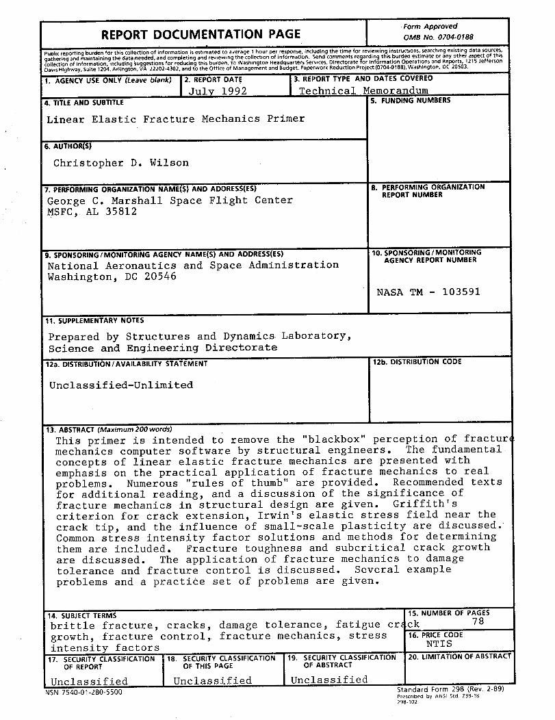
Form Approved
REPORT DOCUMENTATION PAGE OMeNo.07o4-01Sat
Public reporting burden for this collection of information is estimated to average 1 hour per response, including the time for reviewing instructions, searching existing data sources,
gathering and maintain ng the data!needed, and comp et ng and reviewing the collection of informatiOn. Send comments regarding this burden estimate or any other aspect of thiscollection of information, including _uggestions for reducing this burden, to Washington Headquarters Services, Directorate for Information Operations and Reports, 1215 Jefferson
Davis Highway, Suite 1204, Arlington, VA 22202-4302. and to the Office of Management and Budget, Paperwork Reduction Project (0704-0188), Washington, DC 20503.
il. AGENCY USE ONLY (Leave blank) 2. REPORT DAT.E 3. REPORT TYPE AND DATES COVERED
July 1992 Technical Memorandum14. TITLE AND SUBTITLE 5. FUNDING NUMBERS
Linear Elastic Fracture Mechanics Primer
6. AUTHORS)
Christopher D. Wilson
7. PERFORMING ORGANIZATION NAME(S) AND ADDRESS(ES)
George C. Marshall Space Flight Center
MSFC,. AL 35812
9. SPONSORING/MONITORINGAGENCYNAME(S) AND ADDRESS(ES)
National Aeronautics and Space Administration
Washington, DC 20546
8. PERFORMING ORGANIZATIONREPORT NUMBER
10. SPON SORING / MONITORINGAGENCY REPORT NUMBER
NASA TM - 103591
11. SUPPLEMENTARYNOTES
Prepared by Structures and Dynamics. Laboratory,
Science and Engineering Directorate
12a. DISTRIBUTION / AVAILABILITY STATEMENT
Unclassified-Unlimited
12b. DISTRIBUTION CODE
13. ABSTRACT _ax_um 200 words)
This primer is intended to remove the "blackbox" perception of fractur_
mechanics computer software by structural engineers. The fundamental
concepts of linear elastic fracture mechanics are presented with
emphasis on the practical application of fracture mechanics to real
problems. Numerous "rules of thumb" are provided. Recommended textsfor additional reading, and a discussion of the significance of
fracture mechanics in structural design are given. Griffith's
criterion for crack extension, Irwin's elastic stress field near the
crack tip, and the influence of small-scale plasticity are discussed.
Common stress intensity factor solutions and methods for determining
them are included. Fracture toughness and subcritical crack growth
are discussed. The application of fracture mechanics to damagetolerance and fracture control is discussed. Several example
problems and a practice set of problems are given.
14. SUBJECT TERMS
brittle fracture, cracks, damage tolerance, fatigue cr_
growth, fracture control, fracture mechanics, stress
intensity factors17. SECURITY CLASSIFICATION 18. SECURITY CLASSIFICATION
OF REPORT OF THIS PAGE
Unclassified Uncla ssified
NSN 7540-01-280-5500
19. SECURITY CLASSIFICATIONOF ABSTRACT
Unclassified
15. NUMBEROF PAGESck 78
16. PRICE CODE
NTIS
20. LIMITATION OF ABSTRACT
Standard Form 298 (Rev. 2-89)Prescribed by ANSI Std. Z39-18
298-102