Naoyuki Tamura(University of

Durham)

Expected Performance of FMOS ~ Estimation with Spectrum

Simulator ~

Introduction of simulatorsExamples of calculations

Guidelines of detection limits through realisations

Summary

Capability of FMOS

Expected performance ?success rate ??

How detectable and measurable ?

Effects of OH suppression masks ?

Emission / Absorption

How would the spectra look ?

Line flux / centre / width

Spectral coverage : 0.9 ~ 1.8 m

R ~ 500 / ~ 2200

OH airglow suppression mechanism

Let’s perform virtual observation !Web-based

Calculator(http://elvira.phyaig.dur.ac.uk/naoyuki.tamura/ simulator.html) Creates reduced and calibrated spectra.

Quick look at feasibility of your observing program is allowed.

Image SimulatorCreates mock “raw” data (FITS file).

Data reduction and calibration processes can be fully followed.

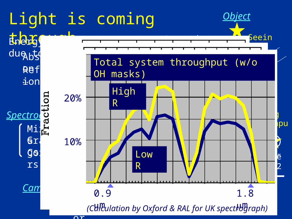
Light is coming through … Atmosphere

Fibre system

FibresFibre connector

Main mirrorPrime focus corrector

Spectrograph

MirrorsGratingsCorrectors

Thermal cut filterDetector

Camera LensesWindow

Sky (Cont.+ OH lines)

Object

Seeing

Energy input

Fibre(1.”25)

AbsorptionReflection…

Energy loss due to :

sec z = 1.5

0.9 m 1.8 m

20%

10%

High R

Low R

(Calculation by Oxford & RAL for UK spectrograph)

Total system throughput (w/o OH masks)

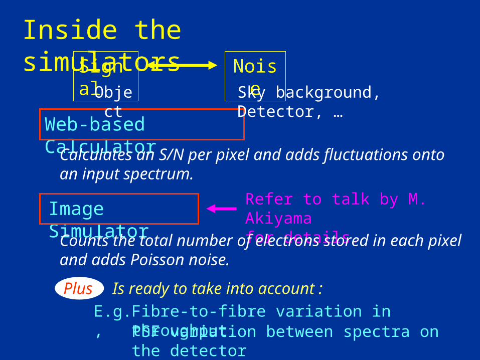
Inside the simulators

Web-based Calculator

Image Simulator

Refer to talk by M. Akiyamafor details.

Calculates an S/N per pixel and adds fluctuations onto an input spectrum.

Signal NoiseObject Sky background, Detector, …

Counts the total number of electrons stored in each pixel and adds Poisson noise.

Is ready to take into account :

Fibre-to-fibre variation in throughput.PSF variation between spectra on the detector

E.g.,

Plus

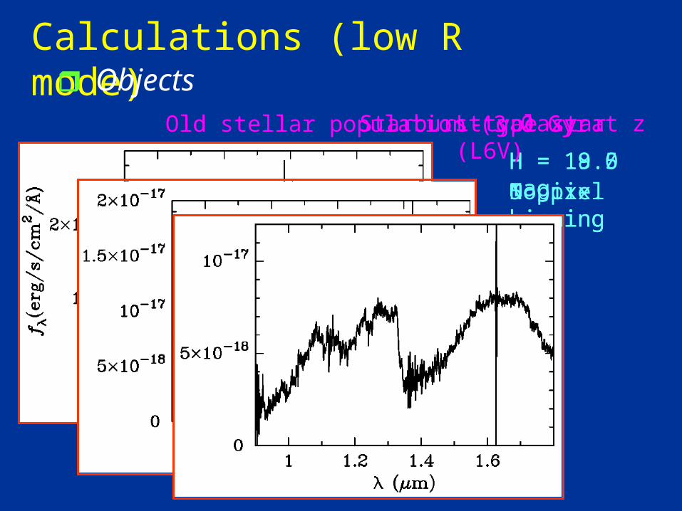
No pix. binning

H = 19.5 magH = 18.0 mag

Calculations (low R mode)Objects

Old stellar population (3.0 Gyr age) at z = 1.5

5 pixel binning

Starburst galaxy at z = 1.5

L-type star (L6V)

4000 A

G-band

H[OII]

[OIII]

H+ [NII]

[SII]H

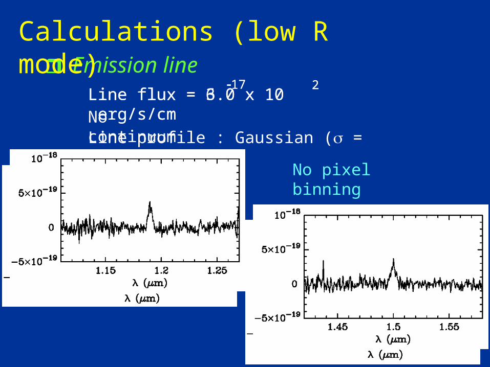
Emission line

No continuumLine profile : Gaussian ( = 300 km/s)

Line flux = 6.0 x 10 erg/s/cm17 2

Calculations (low R mode)

No pixel binning was performed.

Line flux = 3.0 x 10 erg/s/cm17 2

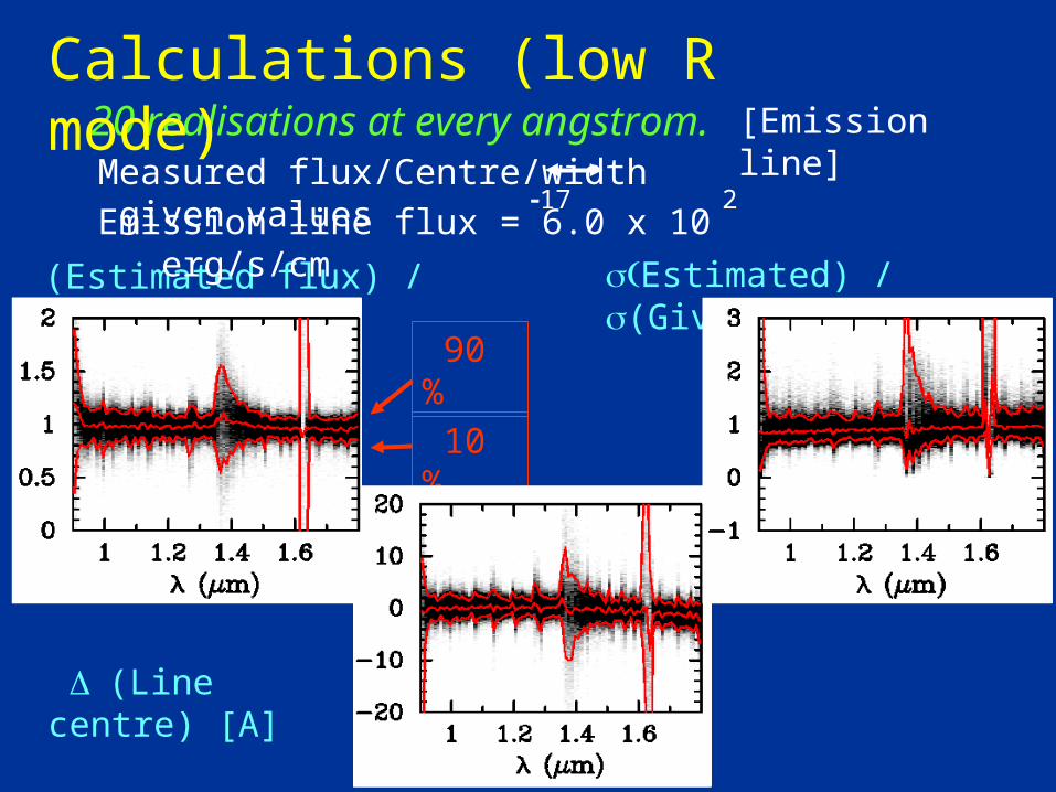
20 realisations at every angstrom.Calculations (low R mode)

Measured flux/Centre/width given values

(Estimated flux) / (Given flux) Estimated) / (Given)

(Line centre) [A]

90 %

10 %

Emission line flux = 6.0 x 10 erg/s/cm17 2

[Emission line]

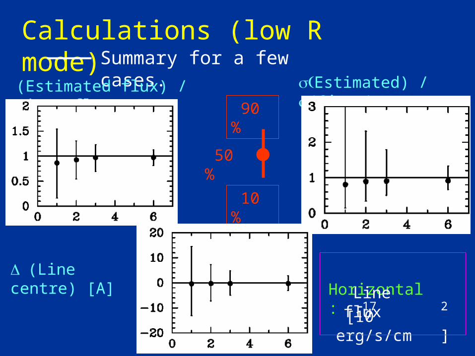
Summary for a few cases.

Calculations (low R mode)

(Estimated flux) / (Given flux) Estimated) / (Given)

(Line centre) [A]

90 %

10 %

Horizontal : Line flux

[10 erg/s/cm ]17 2

50 %

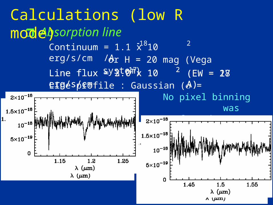
Absorption lineContinuum = 1.1 x 10 erg/s/cm /A

Line profile : Gaussian ( = 300 km/s)

18 2

or H = 20 mag (Vega system)

Line flux = 3.0 x 10 erg/s/cm17 2 (EW = 27 A)

Calculations (low R mode)

No pixel binning was performed.

Line flux = 2.0 x 10 erg/s/cm17 2 (EW = 18 A)

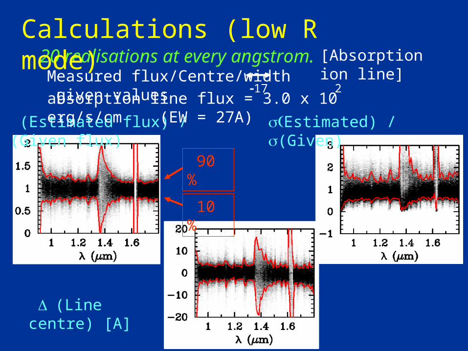
20 realisations at every angstrom.Calculations (low R mode)

(Estimated flux) / (Given flux) Estimated) / (Given)

(Line centre) [A]

90 %

10 %

absorption line flux = 3.0 x 10 erg/s/cm (EW = 27A)17 2

Measured flux/Centre/width given values[Absorption ion line]

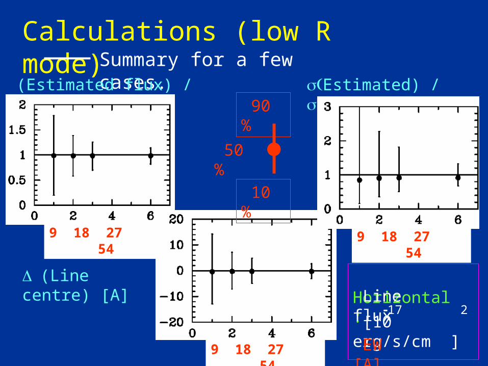
Summary for a few cases.

Calculations (low R mode)

Estimated) / (Given) (Estimated flux) / (Given flux)

(Line centre) [A]

Horizontal : Line flux

[10 erg/s/cm ]17 2

EW [A]

9 18 27 54 9 18 27 54

9 18 27 54

90 %

10 %

50 %

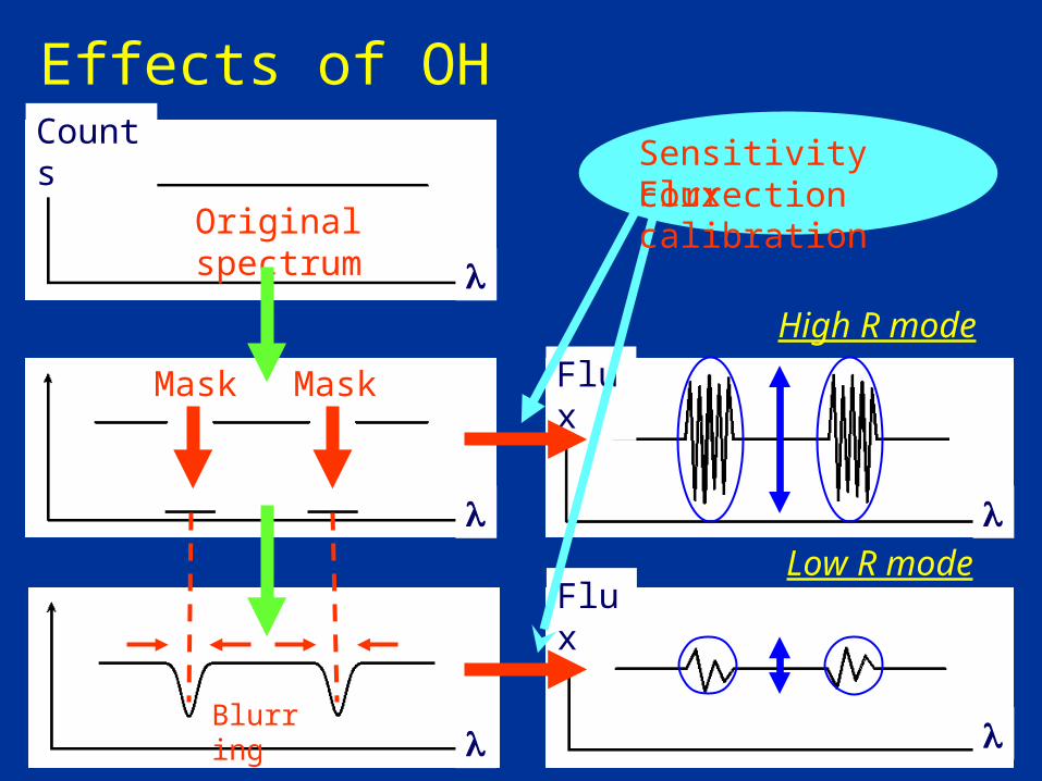
Flux

Flux

Effects of OH masks

Mask Mask

Original spectrum

Sensitivity correctionFlux calibration

Blurring

High R mode

Low R mode

Counts

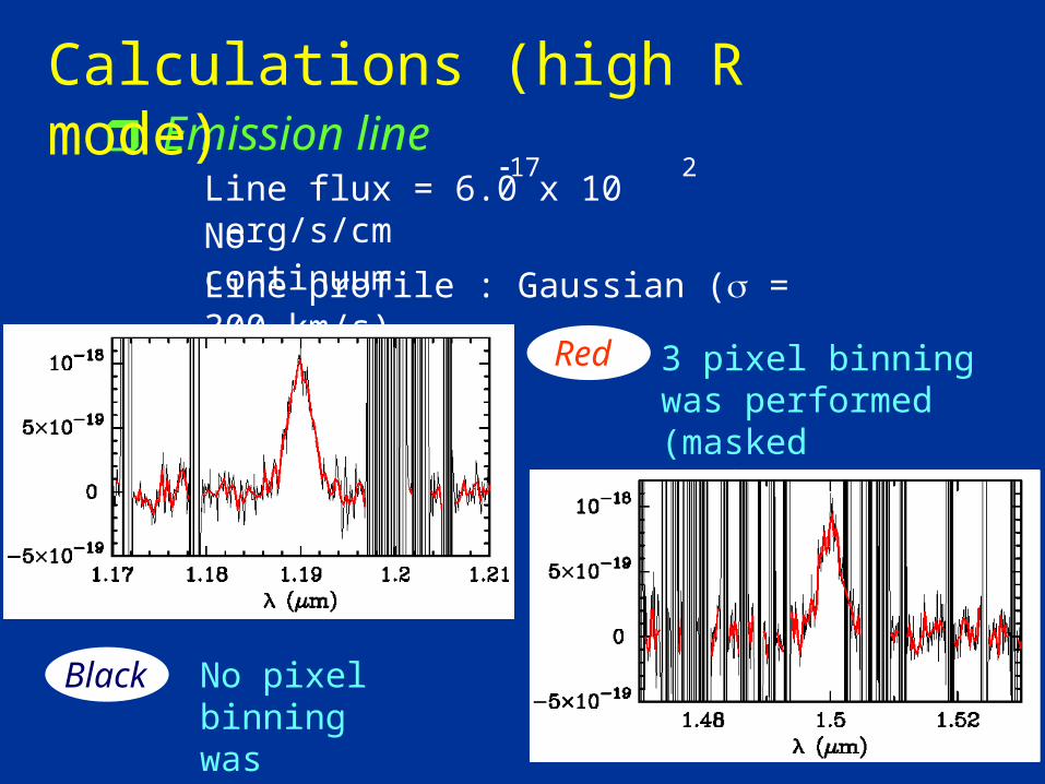
Emission line

No continuum

Line profile : Gaussian ( = 300 km/s)

Line flux = 6.0 x 10 erg/s/cm17 2

Calculations (high R mode)

Black No pixel binningwas performed.

Red 3 pixel binning was performed (maskedregions were avoided).

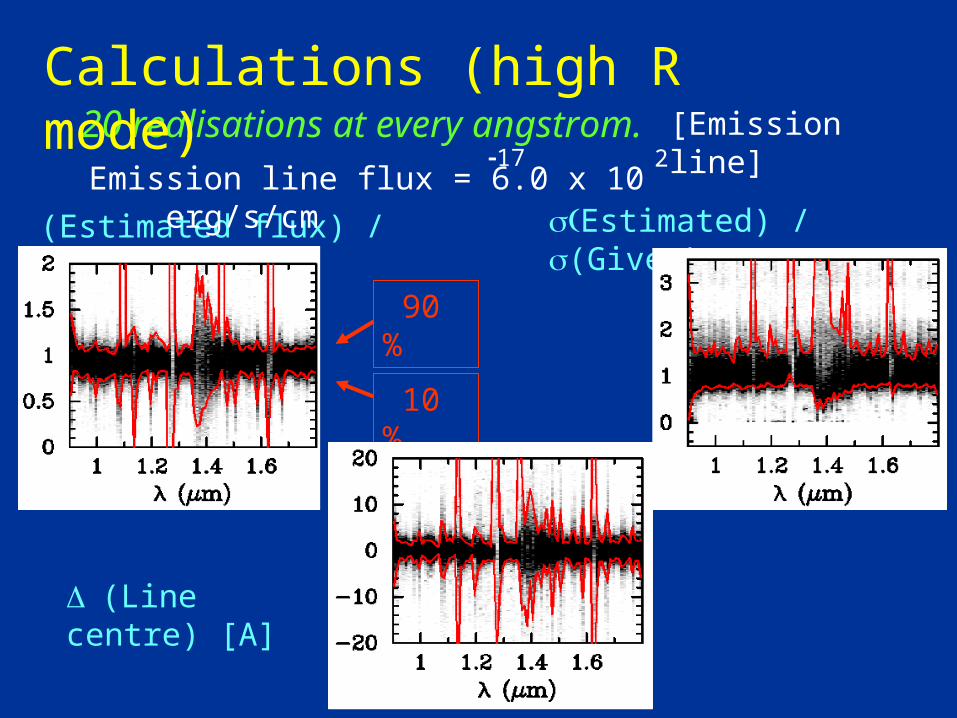
20 realisations at every angstrom.Calculations (high R mode)

(Estimated flux) / (Given flux) Estimated) / (Given)

(Line centre) [A]

90 %

10 %

[Emission line]

Emission line flux = 6.0 x 10 erg/s/cm17 2

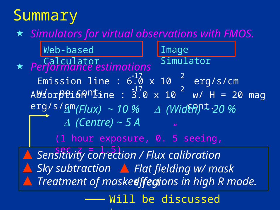
Summary

Will be discussed tomorrow …

(1 hour exposure, 0.”5 seeing, sec z = 1.5)

Simulators for virtual observations with FMOS.

Web-based Calculator

Image Simulator

Performance estimationsEmission line : 6.0 x 10 erg/s/cm w/ no cont.

17 2

Treatment of masked regions in high R mode.

Sensitivity correction / Flux calibration

Absorption line : 3.0 x 10 erg/s/cm17 2

w/ H = 20 mag cont.

Sky subtraction Flat fielding w/ mask effect

(Flux) ~ 10 %(Centre) ~ 5 A

(Width) ~ 20 %