Embed Size (px)
Citation preview
arX
iv:1
806.
0031
2v1
[co
nd-m
at.s
tat-
mec
h] 1
Jun
201
8 Finite-Size Scaling Study of Aging during
Coarsening in Non-Conserved Ising Model: The
case of zero temperature quench
Nalina Vadakkayil, Saikat Chakraborty and Subir K. Das
Theoretical Sciences Unit, Jawaharlal Nehru Centre for Advanced Scientific
Research, Jakkur P.O., Bangalore 560064, India.
E-mail: [email protected]
June 2018
Abstract.
Following quenches from random initial configurations to zero temperature, we
study aging during evolution of the ferromagnetic (nonconserved) Ising model towards
equilibrium, via Monte Carlo simulations of very large systems, in space dimensions
d = 2 and 3. Results for the two-time autocorrelations, obtained by using different
acceptance probabilities for the spin-flip trial moves, are in agreement with each
other. We demonstrate the scaling of this quantity with respect to ℓ/ℓw, where ℓ
and ℓw are the average domain sizes at t and tw (6 t), the observation and waiting
times, respectively. The scaling functions are shown to be of power-law type for
ℓ/ℓw → ∞. The exponents of these power-laws have been estimated via the finite-size
scaling analyses and discussed with reference to the available results from non-zero
temperatures. While in d = 2 we do not observe any temperature dependence, in the
case of d = 3 the outcome for quench to zero temperature is very different from the
available results for high temperature and violates a lower bound, which we explain via
structural consideration. We also present results on the freezing phenomena that this
model exhibits at zero temperature. Furthermore, from simulations of extremely large
system, thereby avoiding the freezing effect, it has been confirmed that the growth of
average domain size in d = 3, that remained a puzzle in the literature, follows the
Lifshitz-Allen-Cahn law in the asymptotic limit.
Keywords: Phase Ordering Dynamics, Aging Phenomena, Ising Model, Monte Carlo,
Finite-size Scaling
Finite-Size Scaling Study of Aging during Coarsening in Non-Conserved Ising Model 2
1. Introduction
Following quench from a homogeneous configuration to a state inside the coexistence
curve, as a system evolves towards the new equilibrium, various structural quantities
exhibit interesting scaling properties [1, 2, 3, 4, 5, 6, 7, 8, 9, 10, 11]. In this context, a
rather general order-parameter correlation function is defined by connecting two space
points (~r1, ~r2) and two times (t, tw), and is written as [2]
C22(~r1, ~r2; t, tw) = 〈ψ(~r1, t)ψ(~r2, tw)〉 −〈ψ(~r1, t)〉〈ψ(~r2, tw)〉. (1)
Here ψ is a space- and time-dependent order-parameter field. For isotropic structures,
which we assume to be true for the cases addressed in this paper, the space dependence
in C22 comes through r = |~r1 − ~r2|, the scalar distance between ~r1 and ~r2. For t = tw,
C22, to be denoted by C(r, t), is referred to as the two-point equal-time correlation
function [1, 2]. On the other hand, for ~r1 = ~r2, we call C22 the two-time autocorrelation
function [2]. The latter quantity, that will be represented by Cag(t, tw), is often used
for studying aging in nonequilibrium systems [2, 3], where tw (≤ t) is referred to as the
waiting time or the age of the system. It is worth mentioning here that Cag(t, tw) may
contain information on relaxation related to equilibration inside individual domains as
well.
The two-point equal-time correlation function typically exhibits the scaling behavior
[1, 2, 9]
C(r, t) ≡ C(r/ℓ(t)), (2)
where C is a time independent master function [1] and ℓ is the average length of domains
that are rich in particles or spins of one or the other type. Usually, ℓ grows in a power-law
manner [1], with exponent α, as
ℓ ∼ tα. (3)
The scaling property in Eq. (2), valid for non-fractal morphology, implies self-similarity,
viz., the structures at two different times differ from each other only by a change in the
length scale [1]. On the other hand, Cag(t, tw), in many situations, exhibits the scaling
form [2, 3, 4, 6, 7, 8, 11, 12, 13]
Cag(t, tw) ≡ Cag(x); x =ℓ
ℓw, (4)
where ℓw is the characteristic length scale of the system at time tw.
There has been serious interest in understanding the forms of these correlation
functions for coarsening dynamics with and without conservation [1, 2] of the total
value of the order parameter (=∫
Vd~rψ(~r, t), V being the system volume). Remarkable
progress has been made with respect to the nonconserved dynamics [1, 2], for scalar
as well as vector order parameters. A large fraction of the studies in the nonconserved
Finite-Size Scaling Study of Aging during Coarsening in Non-Conserved Ising Model 3
variety are related to the coarsening in ferromagnetic Ising model [1, 2] (〈ij〉 stands fornearest neighbors)
H = −J∑
〈ij〉
SiSj , Si = ±1, J > 0, (5)
or in the time-dependent Ginzburg-Landau (TDGL) model [1, 2], the latter being
essentially a coarse-grained version of the kinetic Ising model.
Ohta, Jasnow and Kawasaki (OJK) [9], via a Gaussian approximation of an
auxiliary field [1, 2, 9], obtained an expression for C22 in the case of nonconserved
scalar order-parameter. This reads
C22(r; t, tw) =2
πsin−1 γ, (6)
where
γ =(2
√ttw
t + tw
)d/2
exp[ −r24D(t+ tw)
]
, (7)
d being the system dimension and D a diffusion constant. For t = tw, from Eqs. (6)
and (7) one obtains
C(r, t) =2
πsin−1
[
exp(−r28Dt
)]
. (8)
On the other hand, for r = 0 and t >> tw, we have
Cag(t, tw) ∼( t
tw
)−d/4
. (9)
Given that [1, 2, 14] the value of α is 1/2 for the nonconserved Ising model, Eq. (9)
implies
Cag(t, tw) ∼( ℓ
ℓw
)−λ
; λ =d
2. (10)
Liu and Mazenko (LM) [4], via somewhat similar Gaussian approximation of the
auxiliary field of the order parameter in the TDGL equation, obtained different
dimension dependence for λ. Exact solution of the dynamical equation for C22, that LM
constructed, provides the result same as the OJK one in d = 1. However, (approximate)
solutions of the above mentioned equation in d = 2 and 3 provide [4] λ ≃ 1.29 and
≃ 1.67, respectively.
For the exponent λ, Fisher and Huse (FH) [3] provided the bounds
d
2≤ λ ≤ d. (11)
Notice here that the lower bound of Eq. (11) coincides with the value quoted in Eq. (10),
outcome of the OJK theory. Later, Yeung, Rao and Desai (YRD) [6], by incorporating
the structural differences between the conserved and nonconserved dynamics, obtained
a more general lower bound as
λ >d+ β
2, (12)
Finite-Size Scaling Study of Aging during Coarsening in Non-Conserved Ising Model 4
where β is a power-law exponent related to the small wave-number (k) enhancement of
the structure factor [15, 16]:
S(k, t) ∼ kβ . (13)
It has been shown that β = 0 for nonconserved Ising dynamics [15, 16]. This leads to
the agreement of YRD bound with the FH lower bound. Here note that S(k, t) is the
Fourier transform of C(r, t) and has the scaling form [1, 2]
S(k, t) ≡ ℓdS(kℓ), (14)
where S(kℓ) is a time independent master function.
Predictions of both OJK and LM follow the FH bounds. We mention here that
there exists an argument, related to percolation, by FH [3], that suggests λ = d − a,
where a is the inverse of the exponent for the power-law singularity of the percolation
correlation length. This, e.g., provides λ = 5/4 in d = 2. However, FH [3] cautioned
about using this argument, as well as their upper bound.
Monte Carlo (MC) simulations of the nonconserved Ising model in d = 2 showed
consistency [12, 17] with the OJK function of Eq. (8) and the LM value for λ. The
latter fact appeared true [12, 17] in d = 3 as well, for quenches to certain nonzero
temperatures (Tf ) from the initial temperatures (Ti) that are far above the critical
value (Tc). However, the d = 3 Ising model appears to be different and difficult
[17, 18, 19, 20, 21, 22, 23, 24, 25] for Tf = 0. In this case, simulation reports on
the time dependence of ℓ differ from the theoretical expectation [14]. While some works
reported α = 1/3, a few reported even slower growth. In recent works [22, 25], it has
been shown, via simulations of very large systems, that the (theoretically) expected
value α = 1/2 becomes visible only at very late time.
Furthermore, studies with smaller systems, for Tf = 0, revealed interesting freezing
behavior with respect to reaching the expected ground state [23, 24]. Unusual structural
aspects were also reported for d = 3 [23, 24]. In the structural context, we showed that
C, unlike the d = 2 case, differs from that at high temperatures [17, 26]. Given the
connection between structural and aging properties, discussed above, it is then natural
to ask the question: Does there exist difference in the values of λ for Tf = 0 and Tf > 0?
Our recent letter [26], in fact, suggested the violation of the FH lower bound for Tf = 0 in
d = 3. To confirm that, better analysis of data are needed. Furthermore, even though all
the above mentioned studies of kinetic Ising model use (Glauber) spin-flip [27, 28] as trial
move during the MC simulations [27], that does not preserve the global order parameter,
these moves were accepted with different probabilities in different studies. For example,
in our previous studies, Metropolis algorithm [27] was used, whereas Refs. [23] and [24]
used the Glauber algorithm [27, 28]. Thus, in addition to providing details related to
our recent letter [26] and arriving at appropriate conclusion via more accurate analysis,
we also undertake a comprehensive study to compare results from these two different
algorithms, including results on the freezing phenomena that prevent the systems from
reaching the ground state. Given the anomalies reported at Tf = 0, this exercise, we
feel, is important.
Finite-Size Scaling Study of Aging during Coarsening in Non-Conserved Ising Model 5
In this paper, all the results are presented from Tf = 0. Via state-of-the-art finite-
size scaling analysis [12, 13, 27, 29, 30, 31, 32] of the MC [27] simulation results, we
arrive at the following conclusions for the decay of Cag(t, tw). We confirm that there
exists no temperature dependence in pattern, growth and aging in the case of d = 2. On
the other hand, for d = 3, the value of the aging exponent, estimated from significantly
long period of simulations, indeed violates the FH lower bound. This, however, can be
explained via the structural consideration of YRD. On the issue of freezing, in agreement
with a previous work, we find that for d = 3 and Tf = 0 systems almost never reach
ground state. The frozen length scale, however, is system-size dependent with a linear
relationship. Furthermore, for the domain growth, unambiguous confirmation of the
t1/2 behavior has been provided. Results obtained by using Metropolis and Glauber
algorithms are found to be consistent with each other. Here we state that at Tf = 0
the trial moves that bring no change in the energy are customarily accepted with the
probabilities p = 0, 1/2 or 1, the latter two correspond, respectively, to the Glauber
and Metropolis methods. For p = 0, like the previous studies [23, 24], we observe frozen
dynamics from very early time and these results are not presented.
The rest of the paper is organized as follows. In Section 2 we discuss the methods.
Results are presented in Section 3. Finally we summarize our results in Section 4.
2. Methods
Nonconserved coarsening dynamics in the nearest neighbor Ising model, introduced
above, for Tf = 0, is studied via MC simulations [27] in periodic square (d = 2) and
cubic (d = 3) boxes. We have used square lattice in d = 2 and simple cubic lattice in
d = 3. The values of Tc for this model [27] in d = 2 and 3 are respectively ≃ 2.269J/kBand ≃ 4.51J/kB, kB being the Boltzmann constant.
We have used the Glauber spin-flip moves [28], a standard method to introduce
nonconserved dynamics. For a trial move, the sign of a randomly chosen spin is changed.
The move is accepted if such a change lowers the energy of the system and rejected if
the move increases the energy. For no energy change, one can use different probabilities
p (> 0) for accepting the moves [23, 24]. In this work, we have used p = 0.5 and 1, that
correspond to Glauber [27, 28] and Metropolis [27] acceptance probabilities, respectively.
Time in our simulations was measured in units of MC steps (MCS) [27], one step
consisting of Ld trial moves, L being the linear dimension of a system (in units of the
lattice constant). For the sake of convenience, in the rest of the paper, we set kB, J and
the lattice constant to unity.
For the calculation of length [17], we have identified the sizes, ℓd, of various domains
by scanning a system along different Cartesian directions. Two successive changes in
sign in any direction identify a domain and the corresponding distance provides the
length, i.e., the value of ℓd. The average value, ℓ(t), was obtained from the first moment
Finite-Size Scaling Study of Aging during Coarsening in Non-Conserved Ising Model 6
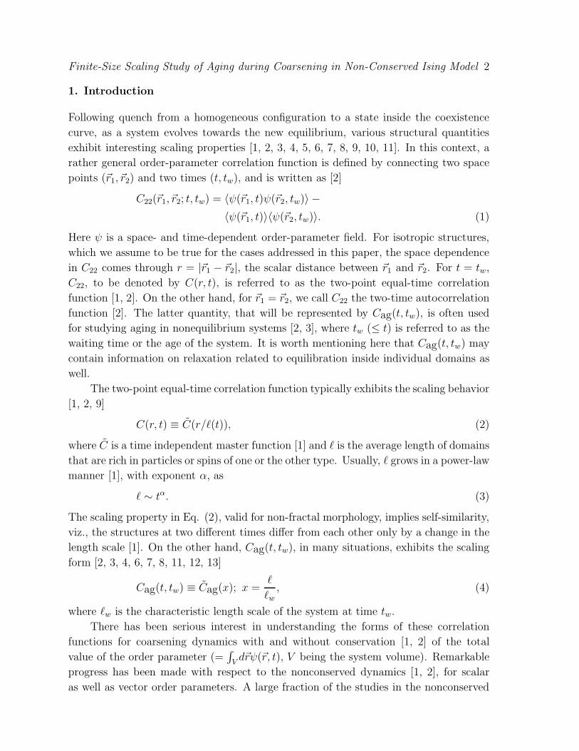
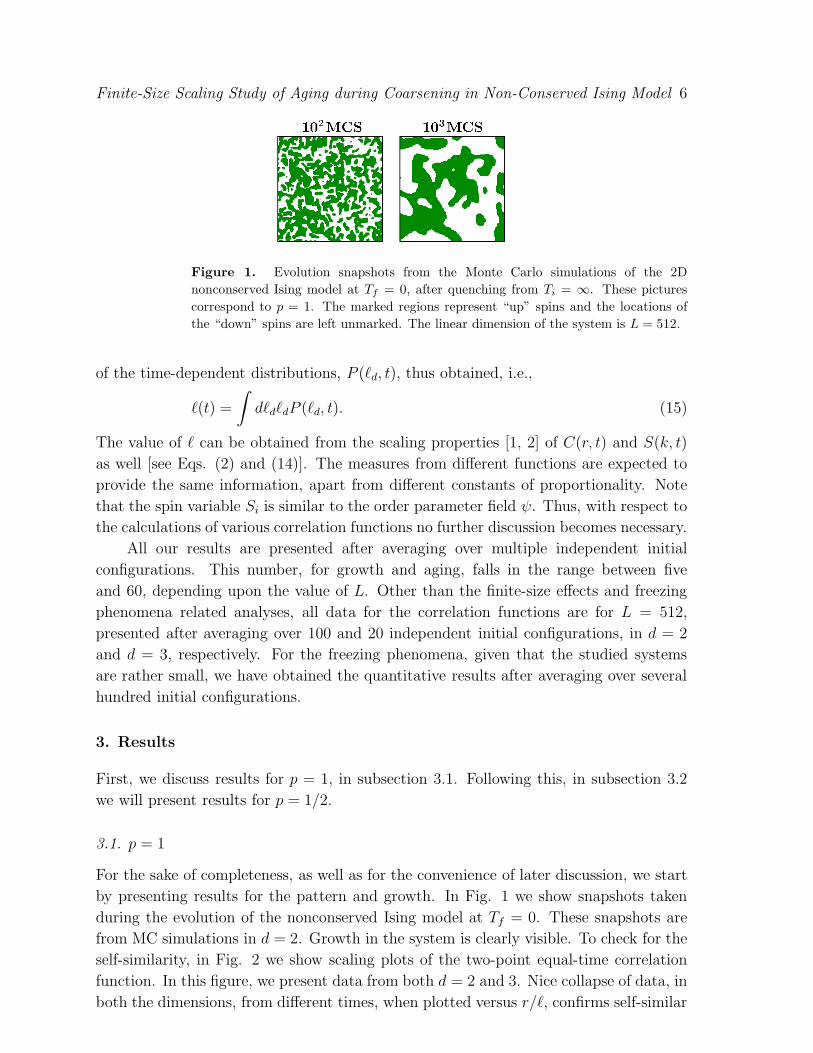
Figure 1. Evolution snapshots from the Monte Carlo simulations of the 2D
nonconserved Ising model at Tf = 0, after quenching from Ti = ∞. These pictures
correspond to p = 1. The marked regions represent “up” spins and the locations of
the “down” spins are left unmarked. The linear dimension of the system is L = 512.
of the time-dependent distributions, P (ℓd, t), thus obtained, i.e.,
ℓ(t) =
∫
dℓdℓdP (ℓd, t). (15)
The value of ℓ can be obtained from the scaling properties [1, 2] of C(r, t) and S(k, t)
as well [see Eqs. (2) and (14)]. The measures from different functions are expected to
provide the same information, apart from different constants of proportionality. Note
that the spin variable Si is similar to the order parameter field ψ. Thus, with respect to
the calculations of various correlation functions no further discussion becomes necessary.
All our results are presented after averaging over multiple independent initial
configurations. This number, for growth and aging, falls in the range between five
and 60, depending upon the value of L. Other than the finite-size effects and freezing
phenomena related analyses, all data for the correlation functions are for L = 512,
presented after averaging over 100 and 20 independent initial configurations, in d = 2
and d = 3, respectively. For the freezing phenomena, given that the studied systems
are rather small, we have obtained the quantitative results after averaging over several
hundred initial configurations.
3. Results
First, we discuss results for p = 1, in subsection 3.1. Following this, in subsection 3.2
we will present results for p = 1/2.
3.1. p = 1
For the sake of completeness, as well as for the convenience of later discussion, we start
by presenting results for the pattern and growth. In Fig. 1 we show snapshots taken
during the evolution of the nonconserved Ising model at Tf = 0. These snapshots are
from MC simulations in d = 2. Growth in the system is clearly visible. To check for the
self-similarity, in Fig. 2 we show scaling plots of the two-point equal-time correlation
function. In this figure, we present data from both d = 2 and 3. Nice collapse of data, in
both the dimensions, from different times, when plotted versus r/ℓ, confirms self-similar
Finite-Size Scaling Study of Aging during Coarsening in Non-Conserved Ising Model 7
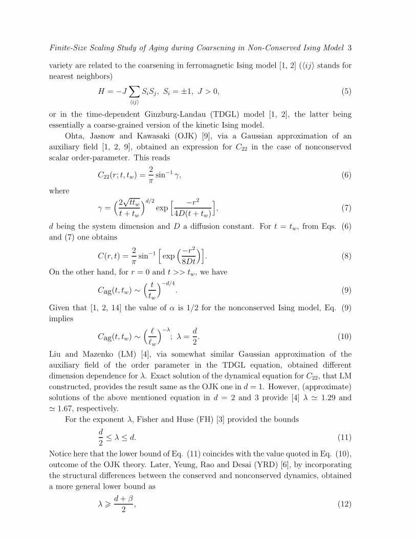
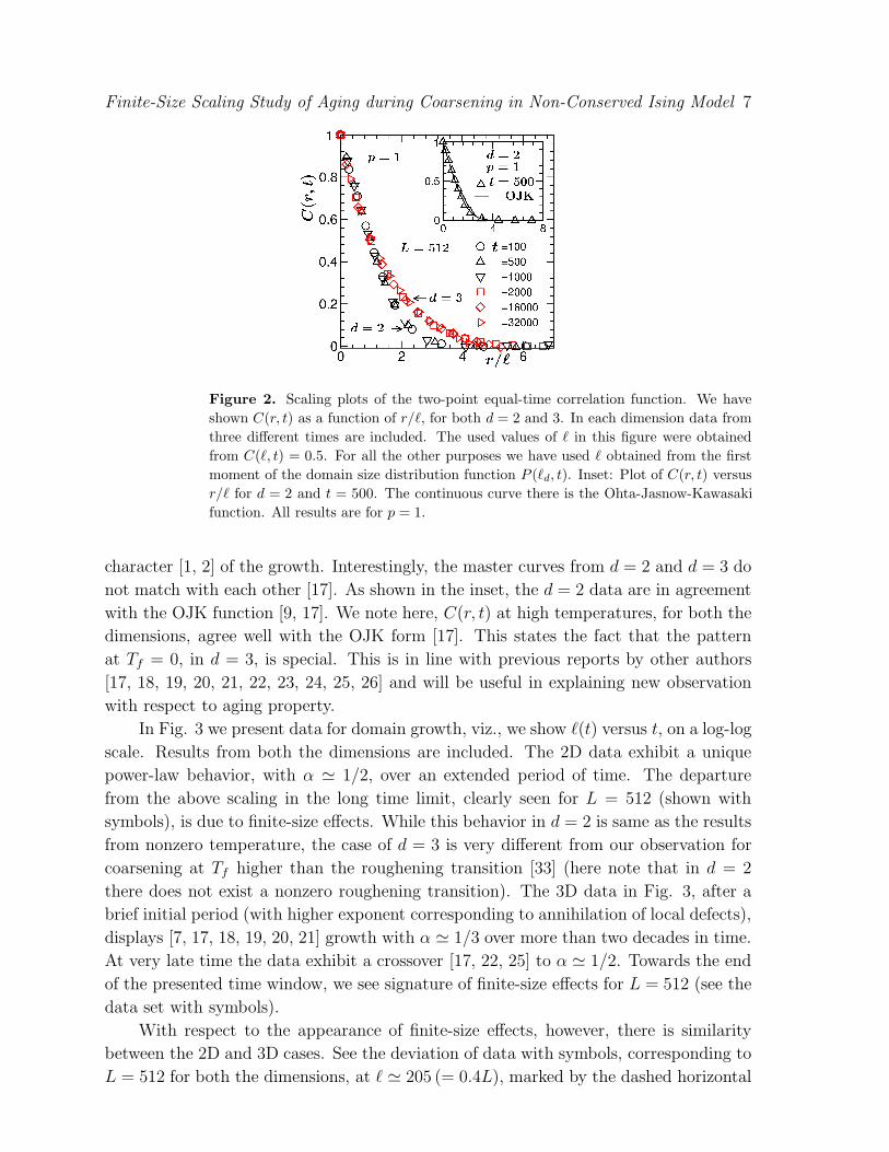
Figure 2. Scaling plots of the two-point equal-time correlation function. We have
shown C(r, t) as a function of r/ℓ, for both d = 2 and 3. In each dimension data from
three different times are included. The used values of ℓ in this figure were obtained
from C(ℓ, t) = 0.5. For all the other purposes we have used ℓ obtained from the first
moment of the domain size distribution function P (ℓd, t). Inset: Plot of C(r, t) versus
r/ℓ for d = 2 and t = 500. The continuous curve there is the Ohta-Jasnow-Kawasaki
function. All results are for p = 1.
character [1, 2] of the growth. Interestingly, the master curves from d = 2 and d = 3 do
not match with each other [17]. As shown in the inset, the d = 2 data are in agreement
with the OJK function [9, 17]. We note here, C(r, t) at high temperatures, for both the
dimensions, agree well with the OJK form [17]. This states the fact that the pattern
at Tf = 0, in d = 3, is special. This is in line with previous reports by other authors
[17, 18, 19, 20, 21, 22, 23, 24, 25, 26] and will be useful in explaining new observation
with respect to aging property.
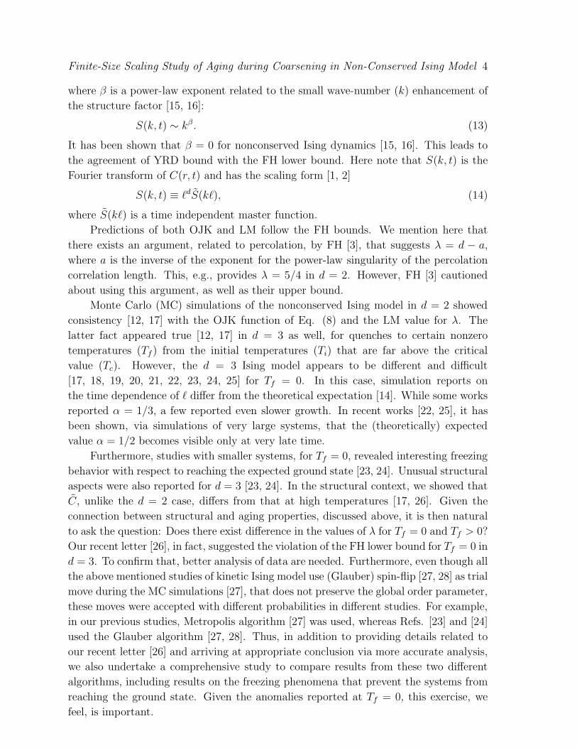
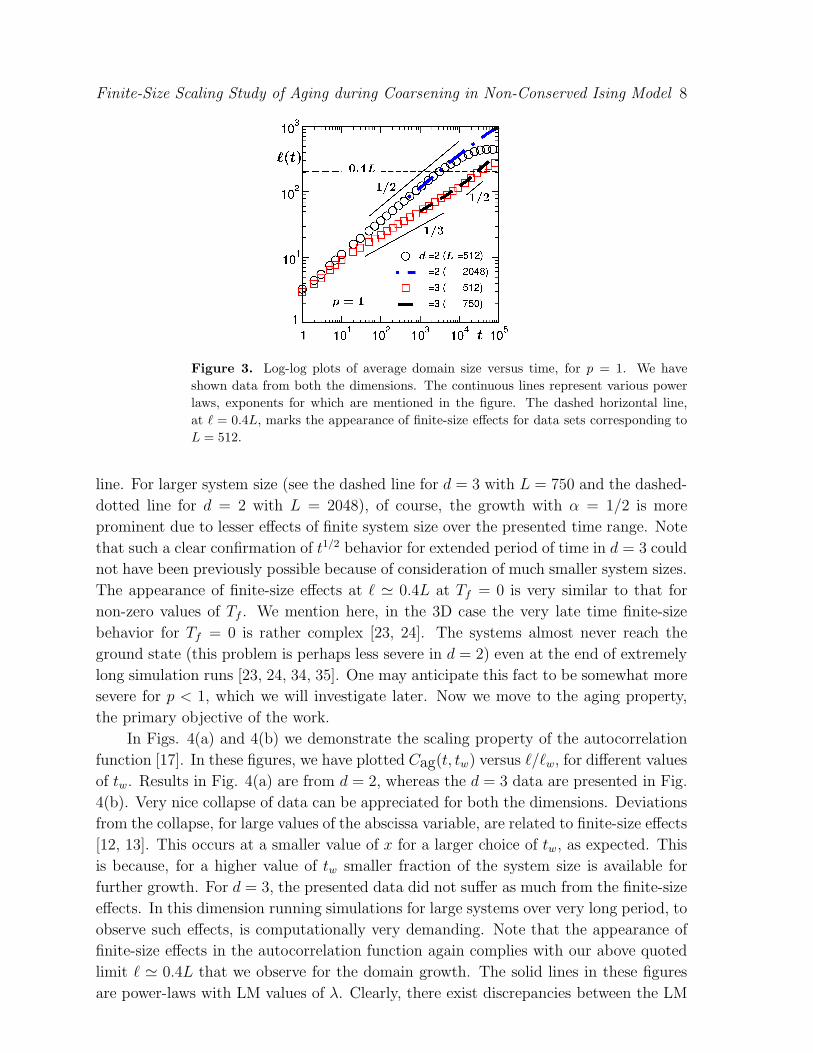
In Fig. 3 we present data for domain growth, viz., we show ℓ(t) versus t, on a log-log
scale. Results from both the dimensions are included. The 2D data exhibit a unique
power-law behavior, with α ≃ 1/2, over an extended period of time. The departure
from the above scaling in the long time limit, clearly seen for L = 512 (shown with
symbols), is due to finite-size effects. While this behavior in d = 2 is same as the results
from nonzero temperature, the case of d = 3 is very different from our observation for
coarsening at Tf higher than the roughening transition [33] (here note that in d = 2
there does not exist a nonzero roughening transition). The 3D data in Fig. 3, after a
brief initial period (with higher exponent corresponding to annihilation of local defects),
displays [7, 17, 18, 19, 20, 21] growth with α ≃ 1/3 over more than two decades in time.
At very late time the data exhibit a crossover [17, 22, 25] to α ≃ 1/2. Towards the end
of the presented time window, we see signature of finite-size effects for L = 512 (see the
data set with symbols).
With respect to the appearance of finite-size effects, however, there is similarity
between the 2D and 3D cases. See the deviation of data with symbols, corresponding to
L = 512 for both the dimensions, at ℓ ≃ 205 (= 0.4L), marked by the dashed horizontal
Finite-Size Scaling Study of Aging during Coarsening in Non-Conserved Ising Model 8
Figure 3. Log-log plots of average domain size versus time, for p = 1. We have
shown data from both the dimensions. The continuous lines represent various power
laws, exponents for which are mentioned in the figure. The dashed horizontal line,
at ℓ = 0.4L, marks the appearance of finite-size effects for data sets corresponding to
L = 512.
line. For larger system size (see the dashed line for d = 3 with L = 750 and the dashed-
dotted line for d = 2 with L = 2048), of course, the growth with α = 1/2 is more
prominent due to lesser effects of finite system size over the presented time range. Note
that such a clear confirmation of t1/2 behavior for extended period of time in d = 3 could
not have been previously possible because of consideration of much smaller system sizes.
The appearance of finite-size effects at ℓ ≃ 0.4L at Tf = 0 is very similar to that for
non-zero values of Tf . We mention here, in the 3D case the very late time finite-size
behavior for Tf = 0 is rather complex [23, 24]. The systems almost never reach the
ground state (this problem is perhaps less severe in d = 2) even at the end of extremely
long simulation runs [23, 24, 34, 35]. One may anticipate this fact to be somewhat more
severe for p < 1, which we will investigate later. Now we move to the aging property,
the primary objective of the work.
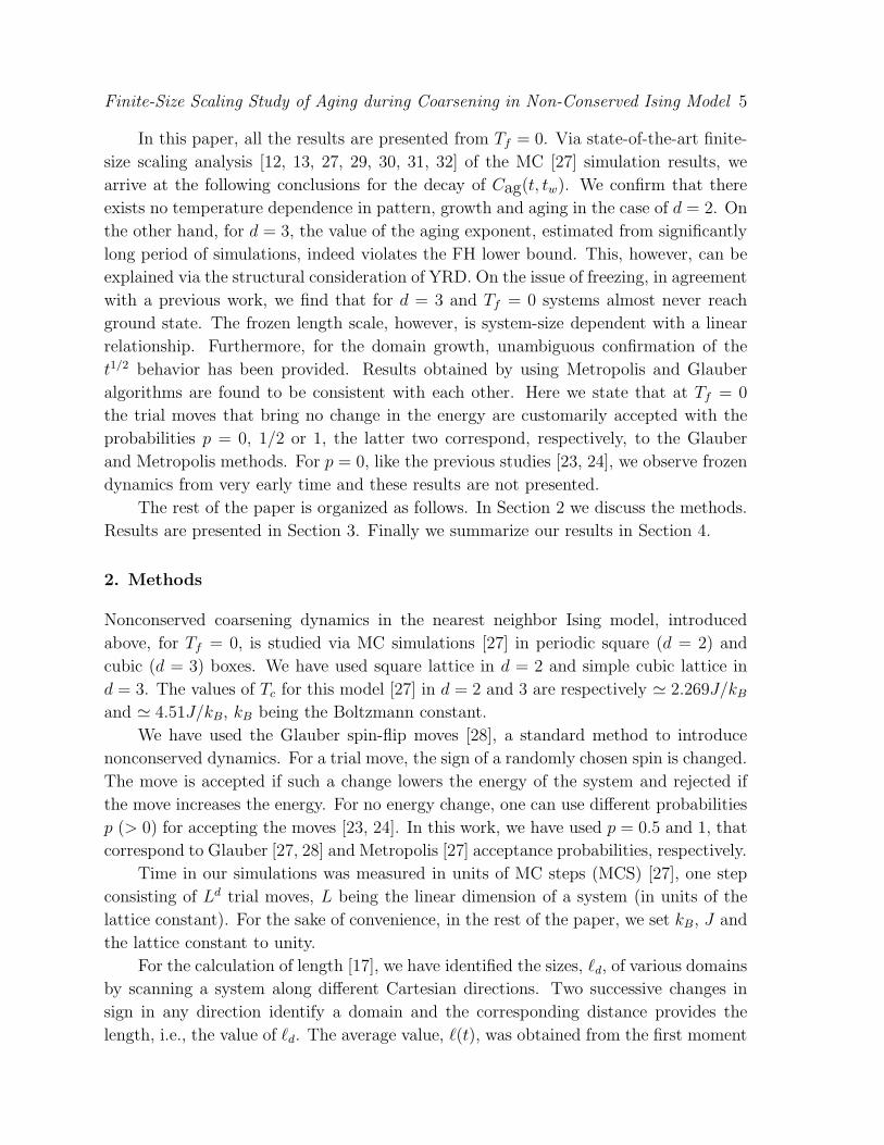
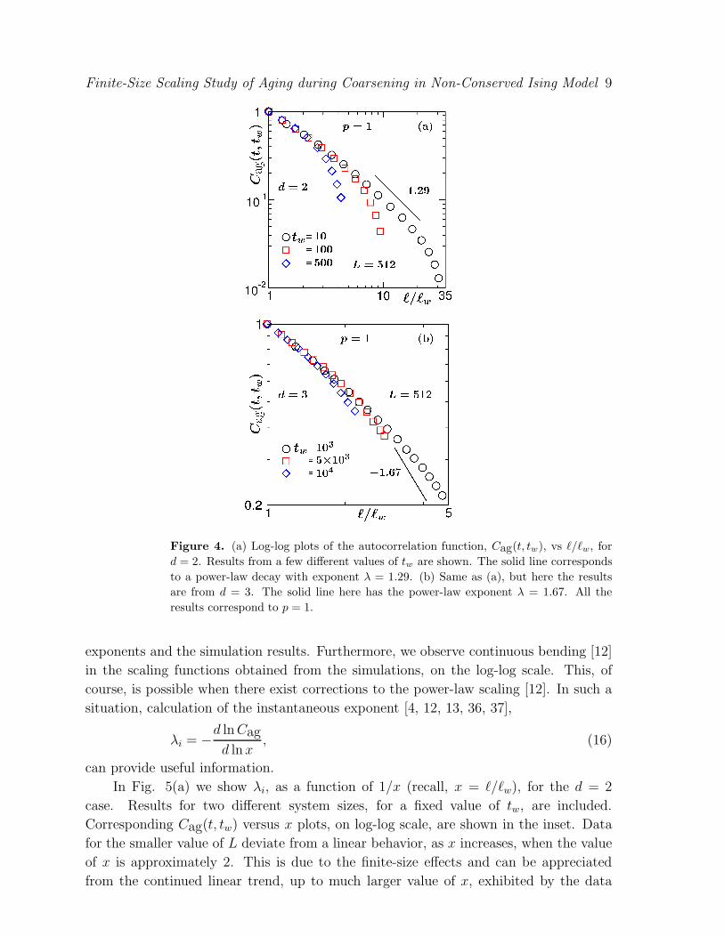
In Figs. 4(a) and 4(b) we demonstrate the scaling property of the autocorrelation
function [17]. In these figures, we have plotted Cag(t, tw) versus ℓ/ℓw, for different values
of tw. Results in Fig. 4(a) are from d = 2, whereas the d = 3 data are presented in Fig.
4(b). Very nice collapse of data can be appreciated for both the dimensions. Deviations
from the collapse, for large values of the abscissa variable, are related to finite-size effects
[12, 13]. This occurs at a smaller value of x for a larger choice of tw, as expected. This
is because, for a higher value of tw smaller fraction of the system size is available for
further growth. For d = 3, the presented data did not suffer as much from the finite-size
effects. In this dimension running simulations for large systems over very long period, to
observe such effects, is computationally very demanding. Note that the appearance of
finite-size effects in the autocorrelation function again complies with our above quoted
limit ℓ ≃ 0.4L that we observe for the domain growth. The solid lines in these figures
are power-laws with LM values of λ. Clearly, there exist discrepancies between the LM
Finite-Size Scaling Study of Aging during Coarsening in Non-Conserved Ising Model 9
Figure 4. (a) Log-log plots of the autocorrelation function, Cag(t, tw), vs ℓ/ℓw, for
d = 2. Results from a few different values of tw are shown. The solid line corresponds
to a power-law decay with exponent λ = 1.29. (b) Same as (a), but here the results
are from d = 3. The solid line here has the power-law exponent λ = 1.67. All the
results correspond to p = 1.
exponents and the simulation results. Furthermore, we observe continuous bending [12]
in the scaling functions obtained from the simulations, on the log-log scale. This, of
course, is possible when there exist corrections to the power-law scaling [12]. In such a
situation, calculation of the instantaneous exponent [4, 12, 13, 36, 37],
λi = −d lnCagd lnx
, (16)
can provide useful information.
In Fig. 5(a) we show λi, as a function of 1/x (recall, x = ℓ/ℓw), for the d = 2
case. Results for two different system sizes, for a fixed value of tw, are included.
Corresponding Cag(t, tw) versus x plots, on log-log scale, are shown in the inset. Data
for the smaller value of L deviate from a linear behavior, as x increases, when the value
of x is approximately 2. This is due to the finite-size effects and can be appreciated
from the continued linear trend, up to much larger value of x, exhibited by the data
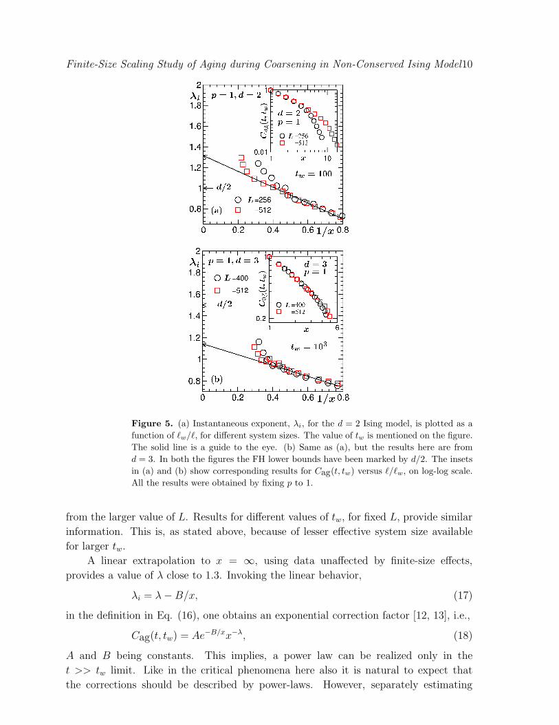
Finite-Size Scaling Study of Aging during Coarsening in Non-Conserved Ising Model10
Figure 5. (a) Instantaneous exponent, λi, for the d = 2 Ising model, is plotted as a
function of ℓw/ℓ, for different system sizes. The value of tw is mentioned on the figure.
The solid line is a guide to the eye. (b) Same as (a), but the results here are from
d = 3. In both the figures the FH lower bounds have been marked by d/2. The insets
in (a) and (b) show corresponding results for Cag(t, tw) versus ℓ/ℓw, on log-log scale.
All the results were obtained by fixing p to 1.
from the larger value of L. Results for different values of tw, for fixed L, provide similar
information. This is, as stated above, because of lesser effective system size available
for larger tw.
A linear extrapolation to x = ∞, using data unaffected by finite-size effects,
provides a value of λ close to 1.3. Invoking the linear behavior,
λi = λ− B/x, (17)
in the definition in Eq. (16), one obtains an exponential correction factor [12, 13], i.e.,
Cag(t, tw) = Ae−B/xx−λ, (18)
A and B being constants. This implies, a power law can be realized only in the
t >> tw limit. Like in the critical phenomena here also it is natural to expect that
the corrections should be described by power-laws. However, separately estimating
Finite-Size Scaling Study of Aging during Coarsening in Non-Conserved Ising Model11
exponents for corrections of different orders is a difficult task. Given the trend of the
data sets, the exponential factor appears to describe the corrections reasonably well.
We will make further comment on the accuracy of this full form later.
Similar linear behavior is observable in Fig. 5(b) where we have presented data
for d = 3 (again, for corresponding Cag(t, tw) versus ℓ/ℓw plots see the inset). In
this case, the data exhibit convergence to a value [26] between 1.1 and 1.2. While for
d = 2 the convergence is consistent with that for higher temperature [12], there exists
serious departure in the case of d = 3 from the LM prediction. Note that the LM
prediction in d = 3 matches well with the conclusions from the simulation studies at
higher temperatures, above the roughening transition [12]. Furthermore, λ ≃ 1.15 is far
below the lower bound of FH.
Even though reasonably accurate estimate is possible from such extrapolations,
one can do better by performing finite-size scaling analysis [12, 13], given that the data
for λi, at large x, may suffer from statistical error and finite-size effects, preventing
unambiguous choice of regions for performing a linear fit. A finite-size data collapse
exercise will be further useful for bringing confidence in the form of Eq. (18), which
essentially is an empirical form.
In a finite-size scaling method one looks for collapse of data from various system
sizes [27, 29, 30]. Such a method for the analysis of the data for autocorrelation function
was recently constructed [12, 13]. See Refs. [38] for more recent work with a different
system. Like in the critical phenomena [27, 29, 30], here also one introduces a scaling
function Y . To make Y independent of system size, we search for a dimensionless
scaling variable y. Since x (= ℓ/ℓw) is already dimensionless, we choose y = x′/x, where
x′ = L/ℓw. This provides
y =L
ℓ. (19)
For the sake of convenience, we intend to write Cag(t, tw) as a function of y. Then,
Cag(t, tw) = Ae−By/yw
(
ywy
)−λ
, (20)
where yw = L/ℓw, i.e., the value of y at t = tw. Next, we write the finite-size scaling
function, a bridge between thermodynamic and finite-size limit behavior, as
Y = Cag(t, tw)eBy/ywyλw. (21)
In the above equation we have absorbed yλ inside Y .
We stress again that the choice of x′ above is driven by the dimension of x and the
fraction of the total system size available to explore, given that the measurement starts
at tw. Coming back to the above comment “fraction of the total system size available to
explore”, we mention that this quoted fact allows a finite-size scaling analysis only via
the variation of tw, without exploring different system sizes. This is because, we state
again, with the variation of tw, the above mentioned fraction varies, providing different
effective system sizes. This fact we will demonstrate by achieving collapse of data from
different values of L and tw.
Finite-Size Scaling Study of Aging during Coarsening in Non-Conserved Ising Model12
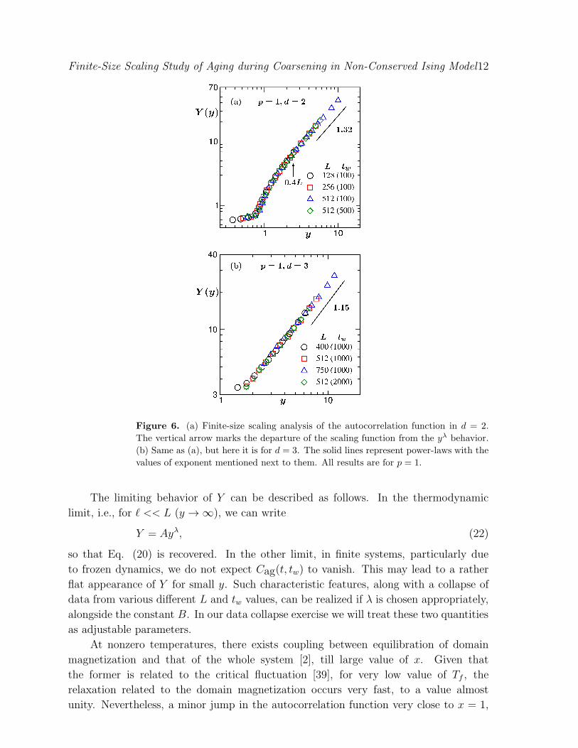
Figure 6. (a) Finite-size scaling analysis of the autocorrelation function in d = 2.
The vertical arrow marks the departure of the scaling function from the yλ behavior.
(b) Same as (a), but here it is for d = 3. The solid lines represent power-laws with the
values of exponent mentioned next to them. All results are for p = 1.
The limiting behavior of Y can be described as follows. In the thermodynamic
limit, i.e., for ℓ << L (y → ∞), we can write
Y = Ayλ, (22)
so that Eq. (20) is recovered. In the other limit, in finite systems, particularly due
to frozen dynamics, we do not expect Cag(t, tw) to vanish. This may lead to a rather
flat appearance of Y for small y. Such characteristic features, along with a collapse of
data from various different L and tw values, can be realized if λ is chosen appropriately,
alongside the constant B. In our data collapse exercise we will treat these two quantities
as adjustable parameters.
At nonzero temperatures, there exists coupling between equilibration of domain
magnetization and that of the whole system [2], till large value of x. Given that
the former is related to the critical fluctuation [39], for very low value of Tf , the
relaxation related to the domain magnetization occurs very fast, to a value almost
unity. Nevertheless, a minor jump in the autocorrelation function very close to x = 1,
Finite-Size Scaling Study of Aging during Coarsening in Non-Conserved Ising Model13
providing a higher effective exponent for very small x, exists. Thus, we avoid the data
point corresponding to x = 1 in all cases, for the finite-size scaling analysis. Furthermore,
scaling of Cag, with respect to ℓ/ℓw, is expected to be observed from rather small values
of tw, very small Tf . Nevertheless, deviations at early time is observed, particularly in
d = 3. This may be due to slow crossover to t1/2 growth behavior extending up to very
late time. Thus, for this scaling analysis, we have chosen rather large values of tw in
this dimension.
Even though in an earlier study [12] (for high temperatures) we have obtained good
data collapse by using finite-size ℓ in the scaling variable y, ideally one should use the
thermodynamic limit values. There can be two possible ways: (i) to adopt ℓ ∼ t1/2
behavior, (ii) to use length from a much larger system size that does not exhibit finite-
size effects over the time-scale of analysis. We follow the latter method here (as well as
for p = 1/2) – for d = 2, ℓ will be taken from L = 2048 and for d = 3, we will use ℓ
from L = 750.
Results from the finite-size scaling analysis for d = 2 are presented in Fig. 6 (a),
whereas corresponding results for d = 3 are presented in Fig. 6 (b). In the case of d = 2,
very good collapse of data, along with consistency with the limiting behavior discussed
above, is obtained for λ = 1.32 and B = 0.80. This value of λ, within statistical
error, is in agreement with a previous study [12] for Tf = 0.6Tc and consistent with
the prediction of LM. In the large y limit the data are consistent with the power-law
amplitude A ≃ 2. This can be appreciated by considering Cag(t, tw) = 1 at x = 1
and B = 0.8. The departure from the power-law behavior is marked by a vertical
arrow in Fig. 6 (a). This corresponds to ℓ = 0.4L where finite-size effects occur. A
robust power law behavior for Y till the finite-size effects appear, irrespective of the
system size, provide confidence in the exponential correction factor. In this connection,
also note that for L = 512 and tw = 100, the power-law behavior extends over t − twranging between 0 and approximately 3600. One may think of improving accuracy in
the estimation of λ by allowing for an adjustable exponent in Eq. (17), by replacing x
by xγ . This exponent will, of course, appear in the argument of the exponential factor.
We caution here that the scaling analysis will be less reliable if γ is included, due to
large number of adjustable parameters. The information with respect to the departure
point of the scaling function from the power-law is quantitatively similar in other cases
as well. So, we will not discuss it again.
For d = 3, on the other hand, the number for the exponent λ turns out to be 1.15,
which is very different from that at 0.6Tc [12]. Again note that the high temperature
result in this dimension is in good agreement with the LM value. Furthermore, the
value of λ at Tf = 0 is far below the lower bound of FH and this conclusion is consistent
with that from the analysis of the instantaneous exponent. The question then comes, is
it a true violation of the bound? This can perhaps be understood from the derivation
of YRD. Before moving to that discussion we briefly point out the intermediate range
features of Y in Fig. 6. Before exhibiting a nearly flat behavior the 2D data fall rather
sharply, compared to the 3D case. This may be related to the more prominent freezing
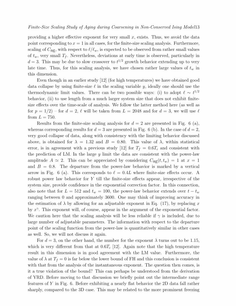
Finite-Size Scaling Study of Aging during Coarsening in Non-Conserved Ising Model14
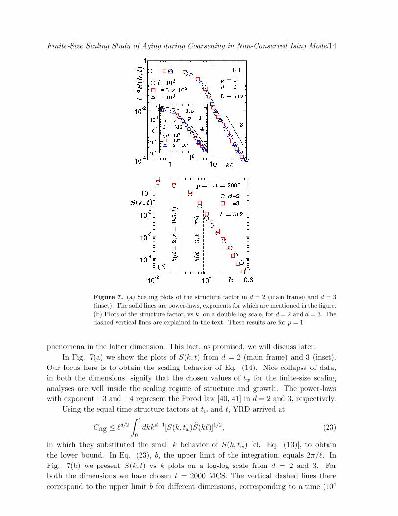
Figure 7. (a) Scaling plots of the structure factor in d = 2 (main frame) and d = 3
(inset). The solid lines are power-laws, exponents for which are mentioned in the figure.
(b) Plots of the structure factor, vs k, on a double-log scale, for d = 2 and d = 3. The
dashed vertical lines are explained in the text. These results are for p = 1.
phenomena in the latter dimension. This fact, as promised, we will discuss later.
In Fig. 7(a) we show the plots of S(k, t) from d = 2 (main frame) and 3 (inset).
Our focus here is to obtain the scaling behavior of Eq. (14). Nice collapse of data,
in both the dimensions, signify that the chosen values of tw for the finite-size scaling
analyses are well inside the scaling regime of structure and growth. The power-laws
with exponent −3 and −4 represent the Porod law [40, 41] in d = 2 and 3, respectively.
Using the equal time structure factors at tw and t, YRD arrived at
Cag ≤ ℓd/2∫ b
0
dkkd−1[S(k, tw)S(kℓ)]1/2, (23)
in which they substituted the small k behavior of S(k, tw) [cf. Eq. (13)], to obtain
the lower bound. In Eq. (23), b, the upper limit of the integration, equals 2π/ℓ. In
Fig. 7(b) we present S(k, t) vs k plots on a log-log scale from d = 2 and 3. For
both the dimensions we have chosen t = 2000 MCS. The vertical dashed lines there
correspond to the upper limit b for different dimensions, corresponding to a time (104
Finite-Size Scaling Study of Aging during Coarsening in Non-Conserved Ising Model15
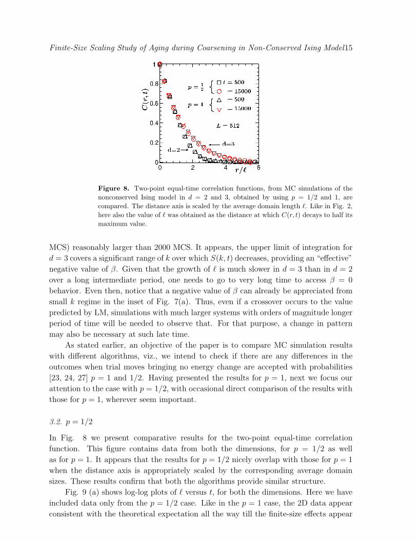
Figure 8. Two-point equal-time correlation functions, from MC simulations of the
nonconserved Ising model in d = 2 and 3, obtained by using p = 1/2 and 1, are
compared. The distance axis is scaled by the average domain length ℓ. Like in Fig. 2,
here also the value of ℓ was obtained as the distance at which C(r, t) decays to half its
maximum value.
MCS) reasonably larger than 2000 MCS. It appears, the upper limit of integration for
d = 3 covers a significant range of k over which S(k, t) decreases, providing an “effective”
negative value of β. Given that the growth of ℓ is much slower in d = 3 than in d = 2
over a long intermediate period, one needs to go to very long time to access β = 0
behavior. Even then, notice that a negative value of β can already be appreciated from
small k regime in the inset of Fig. 7(a). Thus, even if a crossover occurs to the value
predicted by LM, simulations with much larger systems with orders of magnitude longer
period of time will be needed to observe that. For that purpose, a change in pattern
may also be necessary at such late time.
As stated earlier, an objective of the paper is to compare MC simulation results
with different algorithms, viz., we intend to check if there are any differences in the
outcomes when trial moves bringing no energy change are accepted with probabilities
[23, 24, 27] p = 1 and 1/2. Having presented the results for p = 1, next we focus our
attention to the case with p = 1/2, with occasional direct comparison of the results with
those for p = 1, wherever seem important.
3.2. p = 1/2
In Fig. 8 we present comparative results for the two-point equal-time correlation
function. This figure contains data from both the dimensions, for p = 1/2 as well
as for p = 1. It appears that the results for p = 1/2 nicely overlap with those for p = 1
when the distance axis is appropriately scaled by the corresponding average domain
sizes. These results confirm that both the algorithms provide similar structure.
Fig. 9 (a) shows log-log plots of ℓ versus t, for both the dimensions. Here we have
included data only from the p = 1/2 case. Like in the p = 1 case, the 2D data appear
consistent with the theoretical expectation all the way till the finite-size effects appear
Finite-Size Scaling Study of Aging during Coarsening in Non-Conserved Ising Model16
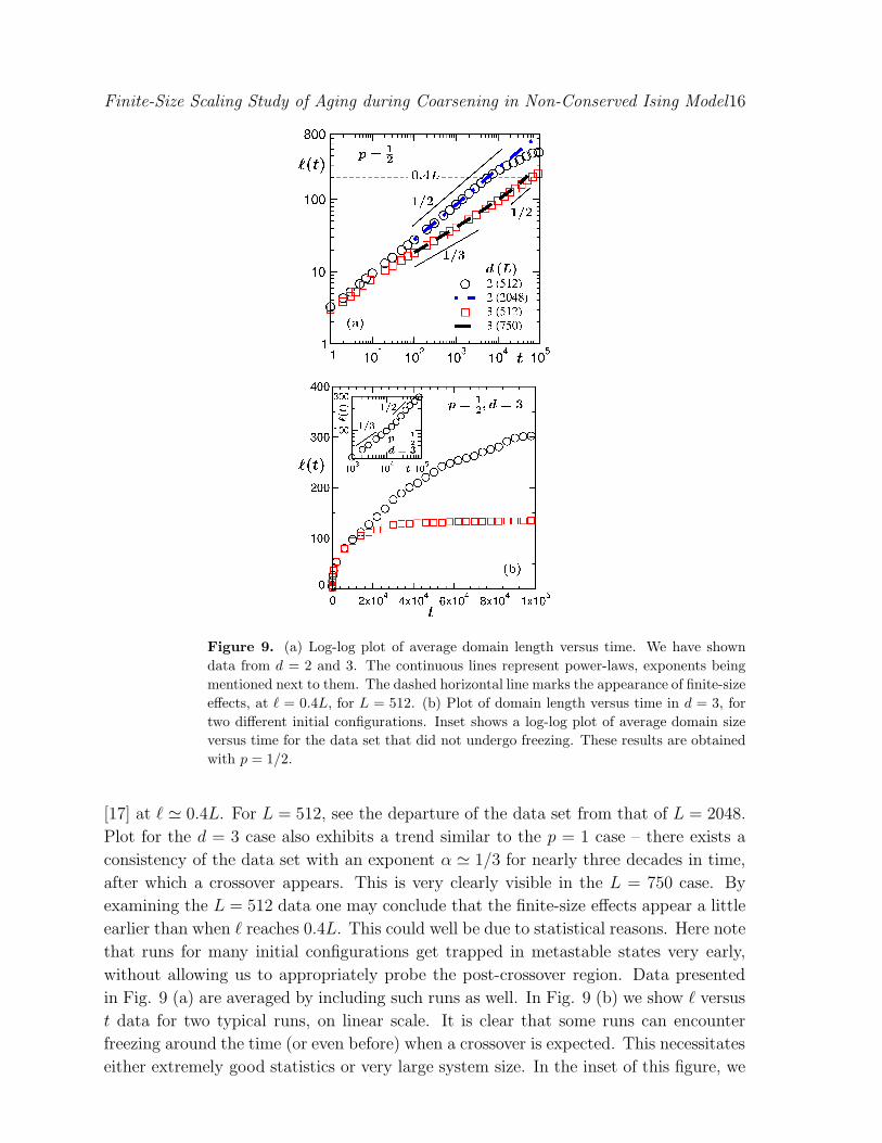
Figure 9. (a) Log-log plot of average domain length versus time. We have shown
data from d = 2 and 3. The continuous lines represent power-laws, exponents being
mentioned next to them. The dashed horizontal line marks the appearance of finite-size
effects, at ℓ = 0.4L, for L = 512. (b) Plot of domain length versus time in d = 3, for
two different initial configurations. Inset shows a log-log plot of average domain size
versus time for the data set that did not undergo freezing. These results are obtained
with p = 1/2.
[17] at ℓ ≃ 0.4L. For L = 512, see the departure of the data set from that of L = 2048.
Plot for the d = 3 case also exhibits a trend similar to the p = 1 case – there exists a
consistency of the data set with an exponent α ≃ 1/3 for nearly three decades in time,
after which a crossover appears. This is very clearly visible in the L = 750 case. By
examining the L = 512 data one may conclude that the finite-size effects appear a little
earlier than when ℓ reaches 0.4L. This could well be due to statistical reasons. Here note
that runs for many initial configurations get trapped in metastable states very early,
without allowing us to appropriately probe the post-crossover region. Data presented
in Fig. 9 (a) are averaged by including such runs as well. In Fig. 9 (b) we show ℓ versus
t data for two typical runs, on linear scale. It is clear that some runs can encounter
freezing around the time (or even before) when a crossover is expected. This necessitates
either extremely good statistics or very large system size. In the inset of this figure, we
Finite-Size Scaling Study of Aging during Coarsening in Non-Conserved Ising Model17
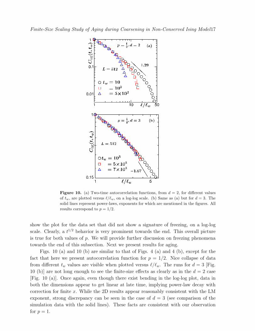
Figure 10. (a) Two-time autocorrelation functions, from d = 2, for different values
of tw, are plotted versus ℓ/ℓw, on a log-log scale. (b) Same as (a) but for d = 3. The
solid lines represent power-laws, exponents for which are mentioned in the figures. All
results correspond to p = 1/2.
show the plot for the data set that did not show a signature of freezing, on a log-log
scale. Clearly, a t1/2 behavior is very prominent towards the end. This overall picture
is true for both values of p. We will provide further discussion on freezing phenomena
towards the end of this subsection. Next we present results for aging.
Figs. 10 (a) and 10 (b) are similar to that of Figs. 4 (a) and 4 (b), except for the
fact that here we present autocorrelation function for p = 1/2. Nice collapse of data
from different tw values are visible when plotted versus ℓ/ℓw. The runs for d = 3 [Fig.
10 (b)] are not long enough to see the finite-size effects as clearly as in the d = 2 case
[Fig. 10 (a)]. Once again, even though there exist bending in the log-log plot, data in
both the dimensions appear to get linear at late time, implying power-law decay with
correction for finite x. While the 2D results appear reasonably consistent with the LM
exponent, strong discrepancy can be seen in the case of d = 3 (see comparison of the
simulation data with the solid lines). These facts are consistent with our observation
for p = 1.
Finite-Size Scaling Study of Aging during Coarsening in Non-Conserved Ising Model18
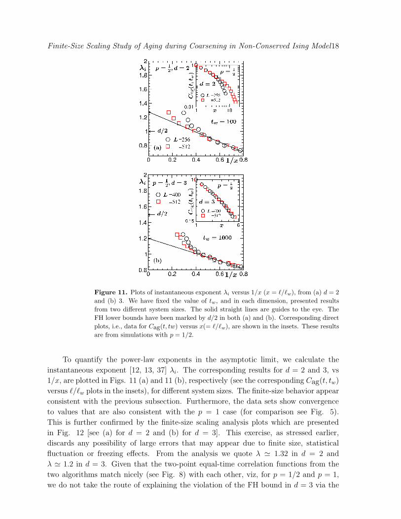
Figure 11. Plots of instantaneous exponent λi versus 1/x (x = ℓ/ℓw), from (a) d = 2
and (b) 3. We have fixed the value of tw, and in each dimension, presented results
from two different system sizes. The solid straight lines are guides to the eye. The
FH lower bounds have been marked by d/2 in both (a) and (b). Corresponding direct
plots, i.e., data for Cag(t, tw) versus x(= ℓ/ℓw), are shown in the insets. These results
are from simulations with p = 1/2.
To quantify the power-law exponents in the asymptotic limit, we calculate the
instantaneous exponent [12, 13, 37] λi. The corresponding results for d = 2 and 3, vs
1/x, are plotted in Figs. 11 (a) and 11 (b), respectively (see the corresponding Cag(t, tw)
versus ℓ/ℓw plots in the insets), for different system sizes. The finite-size behavior appear
consistent with the previous subsection. Furthermore, the data sets show convergence
to values that are also consistent with the p = 1 case (for comparison see Fig. 5).
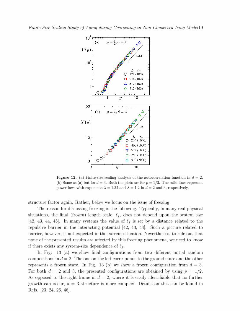
This is further confirmed by the finite-size scaling analysis plots which are presented
in Fig. 12 [see (a) for d = 2 and (b) for d = 3]. This exercise, as stressed earlier,
discards any possibility of large errors that may appear due to finite size, statistical
fluctuation or freezing effects. From the analysis we quote λ ≃ 1.32 in d = 2 and
λ ≃ 1.2 in d = 3. Given that the two-point equal-time correlation functions from the
two algorithms match nicely (see Fig. 8) with each other, viz, for p = 1/2 and p = 1,
we do not take the route of explaining the violation of the FH bound in d = 3 via the
Finite-Size Scaling Study of Aging during Coarsening in Non-Conserved Ising Model19
Figure 12. (a) Finite-size scaling analysis of the autocorrelation function in d = 2.
(b) Same as (a) but for d = 3. Both the plots are for p = 1/2. The solid lines represent
power-laws with exponents λ = 1.32 and λ = 1.2 in d = 2 and 3, respectively.
structure factor again. Rather, below we focus on the issue of freezing.
The reason for discussing freezing is the following. Typically, in many real physical
situations, the final (frozen) length scale, ℓf , does not depend upon the system size
[42, 43, 44, 45]. In many systems the value of ℓf is set by a distance related to the
repulsive barrier in the interacting potential [42, 43, 44]. Such a picture related to
barrier, however, is not expected in the current situation. Nevertheless, to rule out that
none of the presented results are affected by this freezing phenomena, we need to know
if there exists any system-size dependence of ℓf .
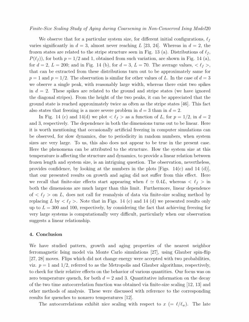
In Fig. 13 (a) we show final configurations from two different initial random
compositions in d = 2. The one on the left corresponds to the ground state and the other
represents a frozen state. In Fig. 13 (b) we show a frozen configuration from d = 3.
For both d = 2 and 3, the presented configurations are obtained by using p = 1/2.
As opposed to the right frame in d = 2, where it is easily identifiable that no further
growth can occur, d = 3 structure is more complex. Details on this can be found in
Refs. [23, 24, 26, 46].
Finite-Size Scaling Study of Aging during Coarsening in Non-Conserved Ising Model20
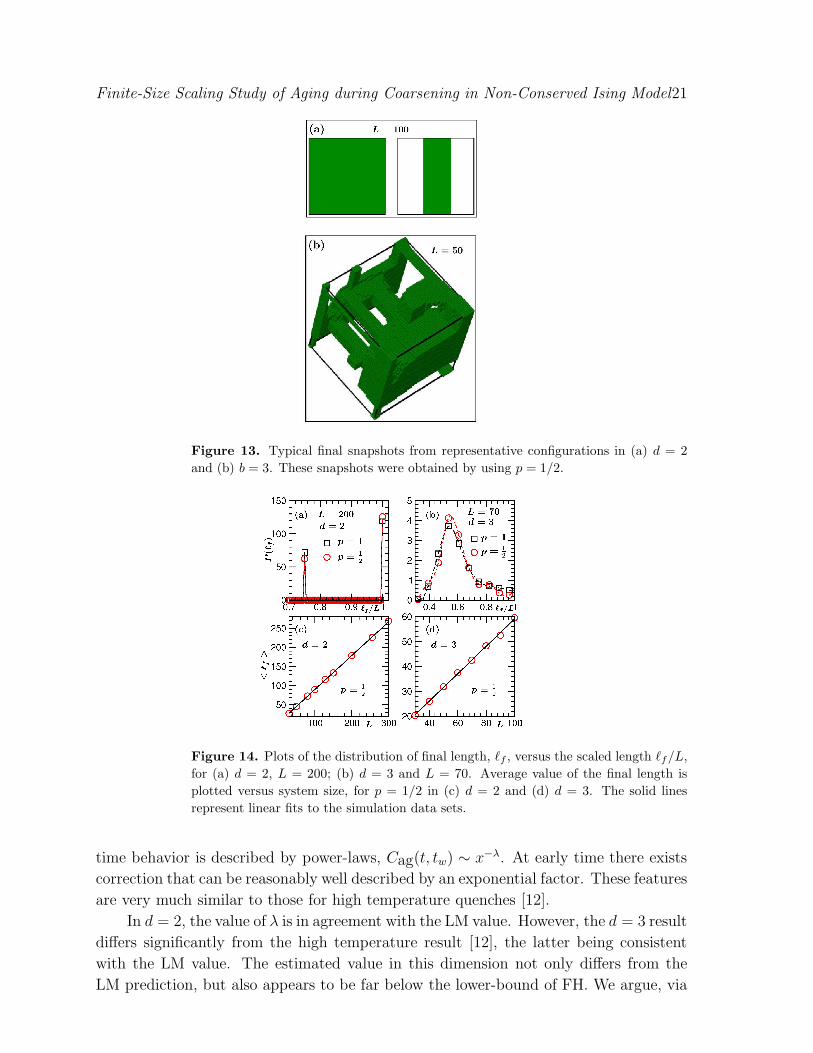
We observe that for a particular system size, for different initial configurations, ℓfvaries significantly in d = 3, almost never reaching L [23, 24]. Whereas in d = 2, the
frozen states are related to the stripe structure seen in Fig. 13 (a). Distributions of ℓf ,
P (ℓf)), for both p = 1/2 and 1, obtained from such variation, are shown in Fig. 14 (a),
for d = 2, L = 200; and in Fig. 14 (b), for d = 3, L = 70. The average values, < ℓf >,
that can be extracted from these distributions turn out to be approximately same for
p = 1 and p = 1/2. The observation is similar for other values of L. In the case of d = 3
we observe a single peak, with reasonably large width, whereas there exist two spikes
in d = 2. These spikes are related to the ground and stripe states (we have ignored
the diagonal stripes). From the height of the two peaks, it can be appreciated that the
ground state is reached approximately twice as often as the stripe states [46]. This fact
also states that freezing is a more severe problem in d = 3 than in d = 2.
In Fig. 14 (c) and 14(d) we plot < ℓf > as a function of L, for p = 1/2, in d = 2
and 3, respectively. The dependence in both the dimensions turns out to be linear. Here
it is worth mentioning that occasionally artificial freezing in computer simulations can
be observed, for slow dynamics, due to periodicity in random numbers, when system
sizes are very large. To us, this also does not appear to be true in the present case.
Here the phenomena can be attributed to the structure. How the system size at this
temperature is affecting the structure and dynamics, to provide a linear relation between
frozen length and system size, is an intriguing question. The observation, nevertheless,
provides confidence, by looking at the numbers in the plots [Figs. 14(c) and 14 (d)],
that our presented results on growth and aging did not suffer from this effect. Here
we recall that finite-size effects start appearing when ℓ ≃ 0.4L, whereas < ℓf > in
both the dimensions are much larger than this limit. Furthermore, linear dependence
of < ℓf > on L, does not call for reanalysis of data via finite-size scaling method by
replacing L by < ℓf >. Note that in Figs. 14 (c) and 14 (d) we presented results only
up to L = 300 and 100, respectively, by considering the fact that achieving freezing for
very large systems is computationally very difficult, particularly when our observation
suggests a linear relationship.
4. Conclusion
We have studied pattern, growth and aging properties of the nearest neighbor
ferromagnetic Ising model via Monte Carlo simulations [27], using Glauber spin-flip
[27, 28] moves. Flips which did not change energy were accepted with two probabilities,
viz. p = 1 and 1/2, referred to as the Metropolis and Glauber algorithms, respectively,
to check for their relative effects on the behavior of various quantities. Our focus was on
zero temperature quench, for both d = 2 and 3. Quantitative information on the decay
of the two time autocorrelation function was obtained via finite-size scaling [12, 13] and
other methods of analysis. These were discussed with reference to the corresponding
results for quenches to nonzero temperatures [12].
The autocorrelations exhibit nice scaling with respect to x (= ℓ/ℓw). The late
Finite-Size Scaling Study of Aging during Coarsening in Non-Conserved Ising Model21
Figure 13. Typical final snapshots from representative configurations in (a) d = 2
and (b) b = 3. These snapshots were obtained by using p = 1/2.
Figure 14. Plots of the distribution of final length, ℓf , versus the scaled length ℓf/L,
for (a) d = 2, L = 200; (b) d = 3 and L = 70. Average value of the final length is
plotted versus system size, for p = 1/2 in (c) d = 2 and (d) d = 3. The solid lines
represent linear fits to the simulation data sets.
time behavior is described by power-laws, Cag(t, tw) ∼ x−λ. At early time there exists
correction that can be reasonably well described by an exponential factor. These features
are very much similar to those for high temperature quenches [12].
In d = 2, the value of λ is in agreement with the LM value. However, the d = 3 result
differs significantly from the high temperature result [12], the latter being consistent
with the LM value. The estimated value in this dimension not only differs from the
LM prediction, but also appears to be far below the lower-bound of FH. We argue, via
Finite-Size Scaling Study of Aging during Coarsening in Non-Conserved Ising Model22
analysis of the structure factor, in line with the derivation of YRD, that this is not a
true violation if the small k behavior of S(k, t) is appropriately accounted for. Here
note that the zero temperature structure in d = 3 is incompatible with the well known
Ohta-Jasnow-Kawasaki form.
As expected, all results are found to be nearly independent of aforementioned
flipping probabilities. This is also true for the freezing property. For the latter we have
demonstrated that the corresponding average length scale varies linearly with the system
size. Close to the frozen length, the dynamics is very slow for d = 3. If an analysis
is performed, to arrive at the domain growth law, via scaling of the corresponding
relaxation time with the system size, a different, misleading conclusion can be arrived
at. Recall that, from simulations of very large systems we confirmed that in this
dimension also the growth at zero temperature follows the Lifshitz-Allen-Cahn law.
We will address this issue of very late time dynamics in a future communication. Before
closing, we mention that despite no dependence of growth exponent on the acceptance
probability p, the growth in the p = 1/2 case is slower than when p is set to unity, due
to higher amplitude in the latter case. This fact is true, as expected, in both the space
dimensions. Our observation suggests that finite-size effects also appear at a slightly
smaller characteristic length scale for p = 1/2.[1] Bray A J 2002 Adv. Phys. 51 481
[2] Puri S and Wadhawan V (eds) 2009 Kinetics of Phase Transitions (CRC Press, Boca Raton)
[3] Fisher D S and Huse D A 1988 Phys. Rev. B 38 373
[4] Liu F and Mazenko G F 1991 Phys. Rev. B 44 9185
[5] Majumdar S N and Huse D A 1995 Phys. Rev. E 52 270
[6] Yeung C, Rao M and Desai R C 1996 Phys. Rev. E 53 3073
[7] Corberi F, Lippiello E and Zannetti M 2006 Phys. Rev. E 74 041106
[8] Henkel M, Picone A and Pleimling M 2004 Europhys. Lett. 68 191
[9] Ohta T, Jasnow D and Kawasaki K 1982 Phys. Rev. Lett. 49 1223
[10] Arenzon J J, Cugliandolo L F and Picco M 2005 Phys. Rev. E 91 032142
[11] Lorenz E and Janke W 2007 Europhys. Lett. 77 10003
[12] Midya J, Majumder S and Das S K 2014 J. Phys. : Condens. Matter 26 452202
[13] Midya J, Majumder S and Das S K 2015 Phys. Rev. E 92 022124
[14] Allen S M and Cahn J W 1979 Acta Metall. 27 1085
[15] Yeung C 1988 Phys. Rev. Lett. 61 1135
[16] Majumdar S N, Huse D A and Lubachevsky B D 1994 Phys. Rev. Lett. 73 182
[17] Das S K and Chakraborty S 2017 Eur. Phys. J. Spec. Top. 226 765
[18] Amar J G and Family F 1989 Bull. Am. Phys. Soc. 34 491
[19] Shore J D, Holzer M and Sethna J P 1992 Phys. Rev. B 46 11376
[20] Lipowski A 1999 Physica A 268 6
[21] Cueille S and Sire C 1997 J. Phys. A 30 L791
[22] Corberi F, Lippiello E and Zannetti M 2008 Phys. Rev. E 78 011109
[23] Olejarz J, Krapivsky P L and Redner S 2011 Phys. Rev. E 83 051104
[24] Olejarz J, Krapivsky P L and Redner S 2011 Phys. Rev. E 83 030104
[25] Chakraborty S and Das S K 2016 Phys. Rev. E 93 032139
[26] Chakraborty S and Das S K 2017 Europhys. Lett. 119 50005
[27] Landau D P and Binder K 2009 A Guide to Monte Carlo Simulations in Statistical Physics,
(Cambridge University Press, Cambridge)
[28] Glauber R J 1963 J. Math. Phys. 4 294
Finite-Size Scaling Study of Aging during Coarsening in Non-Conserved Ising Model23
[29] Fisher M E 1971 Critical Phenomena ed M S Green (Academic, London)
[30] Fisher M E and Barber M N 1972 Phys. Rev. Lett. 28 1516
[31] Heermann D W, Yixue L and Binder K 1996 Physica A 230 132
[32] Das S K 2015 Molecular Simulation 41 382
[33] Van Beijern H and Nolden I 1987 in Structure and Dynamics of Surfaces II: Phenomena, Models
and Methods, Topics in Current Physics, vol. 43 ed W Schommers and P Von Blanckenhagen
(Berlin, Springer)
[34] Spirin V, Krapivsky P L and Redner S 2001 Phys. Rev. E 63 036118
[35] Mullick P and Sen P 2017 Phys. Rev. E 95 052150
[36] Majumder S and Das S K 2010 Phys. Rev. E 81 050102
[37] Huse D A 1986 Phys. Rev. B 34 7845.
[38] Majumder S and Janke W 2016 Phys. Rev. E 93 032506
[39] Fisher M E 1967 Rep. Prog. Phys. 30 615
[40] Porod G 1982 in Small-Angle X-ray scattering ed O Glatter and O Kratky (Academic Press, New
York, 42)
[41] Oono Y and Puri S Mod. Phys. Lett. B 2 861
[42] Das S K 2012 Europhys. Lett. 97 46006
[43] Das S K 2013 Phys. Rev. E 87 012135
[44] Mani E and Lowen H 2015 Phys. Rev. E 92 032301
[45] Tung C, Harder J, Valeriani C and Cacciuto A 2016 Soft Matter 12 555
[46] Olejarz J, Krapivsky P L and Redner S 2012 Phys. Rev. Lett. 109 195702