Embed Size (px)
Citation preview

NADYA T. VINOGRADOVA RUI M. PONTE
Atmospheric and Environmental Research (AER)

1. To examine the relationship between SSS, air-‐sea freshwater fluxes and ocean transports on time scales from months to years.
2. To analyze the potential of satellite-‐derived salinity measurements to constrain surface freshwater flux.

¡ Ocean state estimate is obtained from model/data synthesis produced by the ECCO consortium (Wunsch et al., 2007; 2009)
¡ Fields are computed on a 1° horizontal grid and are diagnosed as monthly averages during 1992-‐2004
¡ SSS refers to salinity averaged over the mixed-‐layer*
*Considering top-‐layer salinity as a measure of SSS did not change our main conclusions

¡ Both F and O give rise to variability in S with O≠0 in many ocean regions ¡ See poster by Vinogradova and Ponte for more discussion
S = F + A + M + E = F + O
*Budget formulation follows Kim et al. (2006)
APPENDIX A
Formulation of SSS balance
Similar to Kim et al. (2004; 2006), the conversation equation for the salinity averaged
vertically along single grid “columns” from the surface (z = 0) to the mixed layer depth
(z = h) is:
∂ [S]
∂t=
(E − P )
h[S]− [∇ · (�uS)] +
�∇ · ( �K)
�− 1
h∆S
∂h
∂t(A1)
where brackets represent vertical average over the varying mixed layer depth h, S is salinity,
�u = (u, v, w) is the three dimensional velocity, �K is the diffusive flux of salt, E − −P
is surface flux of freshwater across the air-sea interface, z is the vertical coordinate, ∇ =
(∂/∂x, ∂/∂y, ∂/∂z), and ∆S is the difference between mixed layer salinity and the salinity
of entrained water.
The right-hand-side terms thus represent tendencies owing to surface forcing (F), advec-
tion (A), mixing (M), and variations in the mixed layer depth (also referred to as “entrain-
ment”, E), respectively. A includes horizontal transports as well as vertical fluxes across
the base of the mixed layer. M includes tendencies due to transports within the mixed
layer as well as mixing across the mixed layer base, and comprises Laplacian, KPP, and
Redi/Gent-McWilliams components. The surface forcing F is the net flux of freshwater de-
fined as evaporation E minus precipitation P . The final term E representing tendencies due
11
psu/mo

¡ Parameterizing O and F as a linear function of S:
(e.g., Dessier and Donguy, 1994; Delcroix et al., 1996; Alory and Delcroix, 1999). The
importance of ocean dynamics is also seen in other ocean regions, where the total balance
represents an interplay between O and F terms of similar amplitudes. In the Indian Ocean,
high variability in S at annual and longer time scales is attributed to both changes in
F , associated with monsoon cycle and river inflow (Boyer and Levitus, 2001), and also to
changes in O, partly under wind-generated Kelvin and Rossby waves (Bruce et al., 1994).
Variability in S in near-coastal regions is influenced by F induced by the outflows of the
major rivers, such as Amazon, Congo, Gange rivers and northern Bay of Bengal, as well
as strong advection and mixing processes within the regions of strong SSS gradients like
western boundary currents.
4. Salinity-derived freshwater flux
Are there regions and time scale where F can be inferred from SSS using simple regres-
sion? As seen from Eqn.(1), O �=0 in many ocean regions and the ability to express F in terms
of S will depend on how well O can be parameterized as a linear function of F . Consider
O as:
O = β · F + εO (2)
where β is linear fit and εO is noise. Then, after substituting (2) to (1) and defying α =
1/(1 + β) and ε=εO/(1+β), F can be expressed as a linear function of S:
3
3. Salinity budget
Similar to SST, SSS in climate studies often refers to the salinity averaged over the ocean
mixed layer (e.g., Qu et al., 2011). The salinity in the mixed layer evolves according to the
conservation equation, stating that the salinity tendency (S) is governed by the atmospheric
(F) and oceanic (O) fluxes, which include tendencies due to advective (A), mixing (M) and
entrainment fluxes of salt (E), and can be written symbolically as follows (see Appendix for
term definitions):
S = F +O
O = A+M+ E (1)
All terms in Eqn.(1) are computed at the model’s integrations time step (1 hour) and
diagnosed as monthly averages. Following formulation developed by Kim et al. (2006) for
entrainment, the salinity budget closes exactly within numerical accuracy of the solution.
Figures 1 and 2 examine variability of budget terms in terms of respective standard
deviations. Many ocean regions are characterized by a complicated balance, with both
atmospheric and oceanic fluxes giving rise to variability in S. For example, both O and
F contribute to the enhanced variability in S in the tropical Pacific and tropical Atlantic.
Here, variability in O is mostly governed by A, partly due to the changes in the flow of
the North Equatorial Counter Current (NECC) that transports lower salinity from west to
east (Donguy and Meyers, 1996). Changes in precipitation under migrating Intertropical
Convergence Zones (ITCZ) in the Atlantic and also the South Pacific Convergence Zone
(SPCZ) in the Pacific are the primary factors of enhanced variability in F in the tropics
2
F = α · S + ε = FS + ε (3)
where ε are residuals between the salinity-derived flux FS=α·S and the “observed” flux F .
The values of α can be determined by regressing F opposite to S (to simplify the analysis,
the offset is set to zero by removing the time mean from both series).
For the linear model (3) to be adequate, the residuals (or their variance) should be small:
ε∼ 0. If oceanic transports are negligible, than Eqn.(1) reduces to the first two terms and
the values of ε represent the noise in the estimates of S and F :
O ∼ 0 : S = F → ε ∼ 0 (4)
In the case of noise-free estimates of S and F (ideal scenario), α = 1 and the flux values can
be derived as FS= S. If, on the other hand, oceanic fluxes are non-negligible, than in oder
to have meaningful values of FS, O and F have to be strongly correlated, otherwise linear
model (3) is not adequate:
O �= 0 :
β · F �= 0 and εO ∼ 0 → ε ∼ 0
β · F = 0 and εO �= 0 → ε �= 0
(5)
Previous attempts to infer F from SSS measurements are typically performed under the
assumption that the role of ocean’s dynamics can be neglected, O∼0 (e.g., Bingham et al.,
2011). Our analysis has a more general approach and examines the possibility of atmospheric
and oceanic terms being parameterized as a linear function of S. We explore such possibility
as a function of time and spatial scale.
4
(1)
¡ For linear model (1) to be adequate: σ2(ε)<<σ2(F) § If (as previously assumed, e.g., Bingham et al. 2011 ), then
§ If (a more general approach), then (1) is valid if O and F are correlated
F = α · S + ε = FS + ε (3)
where ε are residuals between the salinity-derived flux FS=α·S and the “observed” flux F .
The values of α can be determined by regressing F opposite to S (to simplify the analysis,
the offset is set to zero by removing the time mean from both series).
For the linear model (3) to be adequate, the residuals (or their variance) should be small:
ε∼ 0. If oceanic transports are negligible, than Eqn.(1) reduces to the first two terms and
the values of ε represent the noise in the estimates of S and F :
O ∼ 0 : S = F → ε ∼ 0 (4)
In the case of noise-free estimates of S and F (ideal scenario), α = 1 and the flux values can
be derived as FS= S. If, on the other hand, oceanic fluxes are non-negligible, than in oder
to have meaningful values of FS, O and F have to be strongly correlated, otherwise linear
model (3) is not adequate:
O �= 0 :
β · F �= 0 and εO ∼ 0 → ε ∼ 0
β · F = 0 and εO �= 0 → ε �= 0
(5)
Previous attempts to infer F from SSS measurements are typically performed under the
assumption that the role of ocean’s dynamics can be neglected, O∼0 (e.g., Bingham et al.,
2011). Our analysis has a more general approach and examines the possibility of atmospheric
and oceanic terms being parameterized as a linear function of S. We explore such possibility
as a function of time and spatial scale.
4
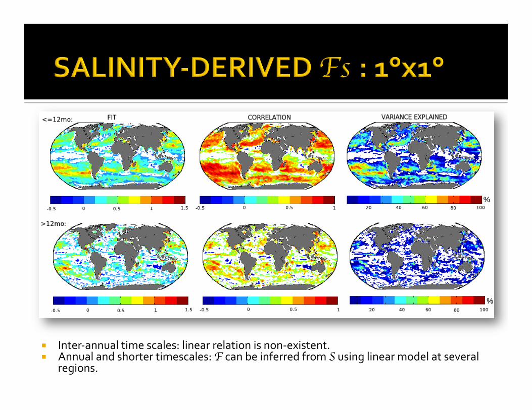
¡ Inter-‐annual time scales: linear relation is non-‐existent. ¡ Annual and shorter timescales: F can be inferred from S using linear model at several
regions.
%
%

¡ For larger spatial scales, we compute Fs based on S and F volume-‐averaged within 20°x20° box
¡ Considering larger spatial scales did not change the results %
Variance explained at 1°x 1°
Variance explained at 20°x 20°
1992 1994 1996 1998 2000 2002 20040.01
0.005
0
0.005
0.01
YEARS
psu/
mo
B
A M E
1992 1994 1996 1998 2000 2002 20040.02
0.01
0
0.01
0.02
YEARS
psu/
mo
A
S F O
1992 1994 1996 1998 2000 2002 20040.02
0.01
0
0.01
0.02
YEARS
psu/
mo
C
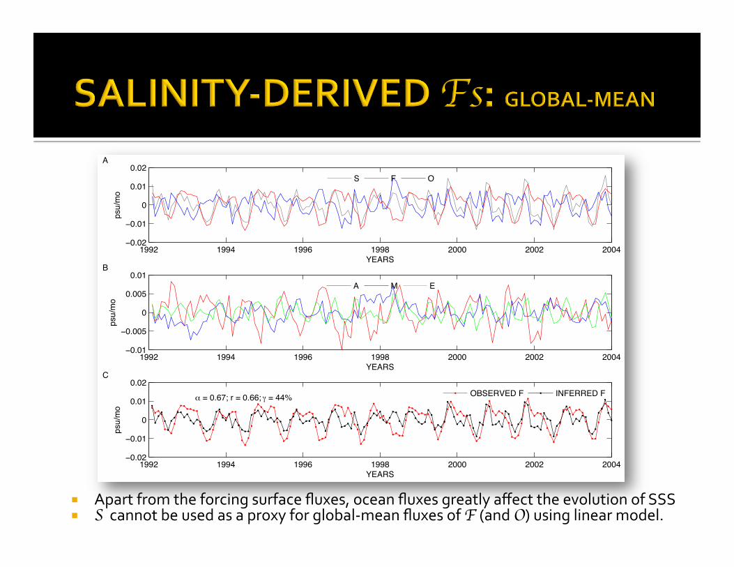
= 0.67; r = 0.66; = 44% OBSERVED F INFERRED F
¡ Apart from the forcing surface fluxes, ocean fluxes greatly affect the evolution of SSS ¡ S cannot be used as a proxy for global-‐mean fluxes of F (and O) using linear model.

Aquarius variability at sub-‐monthly time periods is contaminated by noise
σ(“daily”):
AQUARIUS HYCOM
σ(weekly):
σ(monthly):
σ(daily):
σ(weekly):
σ(monthly):
psu psu
SUB-‐MONTHLY VARIABILITY: (σ2(daily)-‐σ2(monthly))1/2
AQUARIUS
HYCOM
psu

¡ Salt budget analysis show that variability in S can be attributed to both F and O, demonstrating the importance of the ocean's role in evolution of SSS in many regions, particularly through advective fluxes of salt.
¡ There are only a few regions where SSS can be used as a proxy for F and O using linear model, and only at T≤ 12 months.
¡ Notice that the relationship can be different at higher temporal and spatial scales.
¡ Estimates of S and F can be also sensitive to model numerics (mixing schemes, etc).
¡ More sophisticated analysis (e.g., systems like ECCO) might offer a more meaningful estimation of F by assimilation of SSS observations.