NAC-TDDFT: Time-dependent density

functional theory for nonadiabatic couplings

Zikuan Wang, Chenyu Wu and Wenjian Liu∗

Qingdao Institute for Theoretical and Computational Sciences, Institute of Frontier and

Interdisciplinary Science, Shandong University, Qingdao, Shandong 266237, China

E-mail: liuwj@sdu.edu.cn

Conspectus

First-order nonadiabatic coupling matrix elements (fo-NACMEs) are the basic quan-

tities in theoretical descriptions of electronically nonadiabatic processes that are ubiq-

uitous in molecular physics and chemistry. Given the large size of systems of chem-

ical interests, time-dependent density functional theory (TDDFT) is usually the first

choice. However, the lack of wave functions in TDDFT renders the formulation of

NAC-TDDFT for fo-NACMEs conceptually difficult. The present account aims to

analyze the available variants of NAC-TDDFT in a critical but concise manner and

meanwhile point out the proper ways for implementation. It can be concluded, from

both theoretical and numerical points of view, that the equation of motion-based vari-

ant of NAC-TDDFT is the right choice. Possible future developments of this variant

are also highlighted.

1 Introduction

Electronically nonadiabatic processes involving more than one Born-Oppenheimer (BO) po-

tential energy surfaces (PES) are ubiquitous in chemistry, biology and materials science.

1

arX

iv:2

105.

1080

4v1

[ph

ysic

s.ch

em-p

h] 2

2 M

ay 2

021

There exist two mechanisms for these to happen, purely electronic and finite nuclear mass

effects. The former refers to spin-orbit couplings (SOC) responsible for transitions between

electronic states of differen spins, whereas the latter to derivative couplings causing transi-

tions between electronic states of the same spin. To see the latter, we start with the (clamped

nuclei) electronic Schrodinger equation

He|ΨI({ri}; {RA})〉 = EI({RA})|ΨI({ri}; {RA})〉, (1)

He = Te + Vnn({RA}) + Vne({ri}; {RA}) + Vee({ri}), (2)

where the semi-colons emphasize that the nuclear coordinates {RA} are parameters instead

of variables like the electronic coordinates {ri}. The eigenvalues EI({RA}) form PESs on

which the nuclei move. Since {|ΨI({ri})〉} form a complete basis set (CBS), the total wave

function can be expanded as

Φ({ri}, {RA}) =∑J

ΘJ({RA})ΨJ({ri}; {RA}), (3)

which can be inserted into the full Schrodinger equation

(Tn +He)Φ({ri}, {RA}) = EtotΦ({ri}, {RA}) (4)

to obtain the nuclear Schrodinger equation

(Tn + EI({RA})) ΘI({RA}) +∑J

HBOIJ ΘJ({RA}) = EtotΘI({RA}), (5)

2

where

HBOIJ = −

∑ξ

1

Mξ

(gξIJ∂ξ + hξIJ), ∂ξ =d

dξ(6)

gξIJ = 〈ΨI |∂ξ|ΨJ〉, (7)

hξIJ =1

2〈ΨI |∂2ξ |ΨJ〉. (8)

Here, ξ runs over all nuclear degrees of freedom and Mξ is the corresponding atomic mass.

Clearly, the matrix operator HBOIJ vanishes in the limit of infinite nuclear masses. Conversely,

for the true atomic masses, the operator will induce transitions between electronic states of

the same spin, especially when the states are energetically adjacent (cf. Eq. (10) below).

Since the second-order nonadiabatic coupling matrix elements (NACME) (8) can be “trans-

formed away” (without approximation for the considered manifold of PESs) by replacing the

canonical with the kinematic nuclear momentum,1 only the first-order (fo) NACMEs (7) are

relevant. In view of the relation

〈ΨI |[∂ξ, He]|ΨJ〉 = ωJIgξIJ , ωJI = EJ − EI , ∀I 6= J, (9)

the fo-NACMEs can be calculated as

gξIJ =〈ΨI |V ξ

ne|ΨJ〉ωJI

= −gξJI , V ξne = [∂ξ, Vne] = (∂ξVne) (10)

=1

ωJI

∑pq

〈ψp|V ξne|ψq〉γIJpq , γIJpq = 〈ΨI |a†paq|ΨJ〉. (11)

Use of the above Hellmann-Feynman-like expression was first made by Chernyak and Mukamel2

for the fo-NACMEs between the ground and excited states (ge) in the context of time-

dependent density functional theory (TDDFT), which does provide reduced transition den-

sity matrices (rTDM) γIJ between a pair of states. However, even ignoring the fact that the

expression (11) is rooted in (exact) wave function theory (WFT) and hence incompatible

3

with TDDFT, it is hardly useful in practice, for it requires a CBS. For atom-centered basis

sets, the convergence is extremely slow, which can easily be understood by noticing that, as

a real-space function, V ξne has a dipole symmetry and behaves as R−2 in the vicinity of the

nucleus. As such, not only steep p functions but also functions of angular momentum l + 1

have to be added to standard basis functions of angular momentum l.3 A more useful and

simple approach is the finite difference approximation via fast evaluation of the overlap inte-

grals between electronic wave functions at displaced geometries.4,5 However, in total 6Natom

evaluations of the overlap integrals are needed to get the fo-NACMEs and care has to be

taken of the dependence on geometric displacements as well as the phase alignment of the

wave functions. Therefore, analytic NAC-TDDFT should be formulated (see Sec. 2) and

recast into practically useful forms (see Sec. 3). Some numerical results will be provided in

Sec. 4 before concluding the Account in Sec. 5.

The following convention is to be used: {i, j, k, l}, {a, b, c, d} and {p, q, r, s} denote occu-

pied, virtual and arbitrary molecular orbitals (MO), whereas Greek letters refer to atomic

orbitals (AO).

2 NAC-TDDFT

Under the adiabatic approximation, TDDFT amounts to solving the following eigenvalue

problem6

EtI = ωIStI , t†IStJ = δIJ , (12)

where

E =

A B

B A

, S =

I 0

0 −I

, tI =

XI

YI

, (13)

4

Aiaσ,jbτ = δστ (δijFabσ − δabFjiσ) +Kiaσjbτ , (14)

Biaσ,jbτ = Kiaσbjτ , (15)

Kpqσ,rsτ = (pqσ|srτ)− cxδστ (prσ|sqσ) + cxcfxcpqσsrτ [ρ], (16)

Fµνσ = hµν +∑iτ

[(µσνσ|iτ iτ)− cxδστ (µσiτ |iτνσ)] + cxcvxcµνσ[ρ], hµν = Tµν + (Vne)µν . (17)

Here, σ and τ are spin indices. One major issue here is that the eigenvectors of Eq. (12) do

not correspond to excited-state wave functions, but are related to the TDM describing linear

response of the ground state density to an external field (cf. equation (103) in Ref. 7). The

lack of wave functions renders the formulation of TDDFT for fo-NACMEs at least formally

difficult. In the next subsections, the auxiliary/pseudo wave function (AWF), equation of

motion (EOM), and time-dependent response/perturbation theory (TDPT) based formula-

tions are analyzed sequentially.

2.1 AWF-based formulation

To draw analogy with WFT, we start with the Tamm-Dancoff approximation (TDA) to Eq.

(12),

AXI = ωIXI . (18)

If Hartree-Fock (HF) is used as the functional, the A matrix (14) is just the Hamiltonian

matrix in the manifold of singly excited configurations {|Ψai 〉 = a†aai|ΨHF〉}. Therefore, in

this case, the eigenvector XI represents simply the coefficients of the CIS (configuration

interaction singles) wave function ΨCISI ,

|ΨCISI 〉 =

∑ia

|Ψai 〉(XI)ia. (19)

5

Extending the above to an arbitrary functional leads to

|ΨTDAI 〉 =

∑ia

(XI)iaa†aai|ΨKS〉, (20)

which can be termed “auxiliary wave function” (AWF). In this way, the ge and ee (excited

state-excited state) fo-NACMEs can readily be obtained as

gξ0I =∑ia

〈ψi|∂ξ|ψa〉(XI)ia, (21)

gξIJ =∑iab

(XI)ia(XJ)ib〈ψa|∂ξ|ψb〉 −∑ija

(XI)ia(XJ)ja〈ψj|∂ξ|ψi〉. (22)

However, these are not yet the final working equations, as they involve nuclear derivatives

of the MOs, which must be either calculated directly from coupled-perturbed KS (CPKS)

equations or eliminated by the Z-vector approach (see Sec. 3).

The situation becomes very different for the full TDDFT, which has no direct analogy

with any WFT. One common practice is to construct a CIS-like wave function that repro-

duces some property (e.g., electric polarizability) in a sum-of-states form, and then feed it

to Eq. (7). Different choices of properties then lead to different expressions, e.g.,

gξ0I =∑ia

(XI + YI)ia〈ψi|∂ξ|ψa〉, (23)

and

gξ0I =∑ia

(XI −YI)ia〈ψi|∂ξ|ψa〉, (24)

were proposed by Tavernelli8 and Hu,9,10 respectively, for the ge fo-NACMEs. Even more

choices are possible for the ee fo-NACMEs.8,11,12 Due to the lack of theoretical rigor, there is

no a priori argument to favor one over another. In particular, there is no a priori guarantee

that any of them is exact if both the functional and kernel were exact. It is shown in the

next subsections that NAC-TDDFT can indeed be formulated more properly.13–17

6

2.2 EOM-based formulation

In the EOM formalism,18 one defines an excitation operator O†I that promotes the ground

state to an excited state

|I〉 = O†I |0〉, (25)

and is subject to the killer condition

〈0|O†I = 0. (26)

After determining O†I by the EOM

1

2〈0|[δOI , [He, O

†I ]] + [[δOI , He], O

†I ]|0〉 = ωI〈0|[δOI , O

†I ]|0〉, ωI = EI − E0, (27)

the ge and ee matrix elements of an arbitrary operator O can be calculated as

〈0|O|I〉 = 〈0|OO†I |0〉 (28)

= 〈0|[O,O†I ]|0〉, (29)

〈I|O|J〉 = 〈0|OIOO†J |0〉 (30)

=1

2〈0|[OI , [O,O

†J ]]− [[O,OI ], O

†J ]|0〉, I 6= J. (31)

Note that use of the killer condition (26) has been made when going from Eq. (28)/(30) to

(29)/(31), to be consistent with the structure of Eq. (27).

Consider, e.g., the random phase approximation (RPA) with

O†I =∑ia

(XI)iaa†aai − (YI)iaa

†iaa. (32)

It can readily be checked that Eq. (27) with (32) is just Eq. (12) with cx = 1 and cxc = 0,

which can simply be translated to TDDFT with a functional other than HF. Note, however,

7

the O†I operator (32) does not satisfy the killer condition due to the presence of a†iaa. As

such, in principle Eqs. (28) and (30) should be used for the RPA/TDDFT ge and ee matrix

elements, respectively. The resulting expressions are then the same as those by the previous

CIS/TDA-based approach. The very trick for nonvanishing deexcitation amplitudes YI is

still to use Eqs. (29) and (31). Straightforward derivations then yield

〈I|O|J〉 = 〈I|O|J〉0 + 〈I|O|J〉1, (33)

〈I|O|J〉0 =∑pq

γIJpq 〈ψp|O|ψq〉, (34)

〈I|O|J〉1 =1

2〈0|[OI , [O,O

†J ]1]− [[O,OI ]1, O

†J ]|0〉, (35)

[O,O†J ]1 =∑ia

[O, (XI)ia]a†aai − [O, (YI)ia]a

†iaa. (36)

where 〈I|O|J〉1 appears only if O contains nuclear derivatives, and the ge and ee TDMs are

defined in Eqs. (37) and (38), respectively,

γ0Iia = (XI)ia, γ0Iai = (YI)ia, γ0Iij = γ0Iab = 0, (37)

γIJij = −∑a

[(XJ)ia(XI)ja + (YI)ia(YJ)ja] , (38a)

γIJab =∑i

[(XI)ia(XJ)ib + (YJ)ia(YI)ib] , (38b)

γIJia = γIJai = 0. (38c)

Some remarks are in order.

(1) It is the use of the nested commutators of the form [OI , [O,O†J ]] that allows the deex-

citation amplitudes YI to contribute to the matrix elements of O. Such commutators

are only present in EOM but not in the Schrodinger equation itself, which explains the

difficulty of formulating a unique AWF for TDDFT, except for the TDA variant.

8

(2) The ge transition matrix element 〈0|O|I〉0 defined by Eqs. (34) and (37) can be simplified

to

〈0|O|I〉0 =∑ia

(XI + YI)ia〈ψi|O|ψa〉 (39)

if O is real Hermitian or to

〈0|O|I〉0 =∑ia

(XI −YI)ia〈ψi|O|ψa〉 (40)

if O is real anti-Hermitian. The important corollary is that, in the AWF-based approach,

one should construct the AWF with XI + YI in the case of O = V ξne or r but with

XI −YI in the case of O = ∂ξ. This is related to the well-known fact that A+B serves

as the orbital Hessian for responses to a real (“electric”) perturbation, whereas A −B

for responses to a purely imaginary (“magnetic”) perturbation (which is related to real

anti-Hermiticity scaled by the imaginary factor i). As such, TDDFT does not admit a

unique AWF,19,20 as the form of the AWF depends on the type of perturbation studied.

The AWF constructed to reproduce the dipole polarizability (i.e., XI + YI) gives rise

to incorrect ge fo-NACMEs in view of Eq. (40) with O = ∂ξ, whereas the same AWF

used for 〈ΨI |V ξne|ΨJ〉 in Eq. (11) will yield the correct fo-NACMEs, but only in the CBS

limit.

(3) None of the AWF-based methods can reproduce the ee fo-NACMEs obtained by EOM,

unless further approximations are made.12 For example, starting with an AWF XI±YI ,

one obtains

〈I|O|J〉0 =∑iab

(XI±YI)ia(XJ±YJ)ib〈ψa|O|ψb〉−∑ija

(XI±YI)ia(XJ±YJ)ja〈ψj|O|ψi〉,

(41)

which involves cross terms like (XI)ia(YJ)ib not present in the EOM expression (see Eqs.

(34) and (38)).

9

(4) The second term in Eq. (33) with O = ∂ξ has been derived before13 and is hence not

repeated here. The final expressions for the ge and ee fo-NACMEs read

〈0|∂ξ|I〉 =∑ia

(XI −YI)ia〈ψi|∂ξ|ψa〉, (42)

〈I|∂ξ|J〉 =∑pq

γIJpq 〈ψp|∂ξ|ψq〉+ ω−1JI t†I(∂ξE)tJ . (43)

Clearly, the AWF-based expression (24)9,10 happens to be correct but the expression

(23)8 should be rejected.

Albeit elegant, the above EOM-based formulation of fo-NACMEs is still not satisfactory,

for the killer condition (26) does not hold strictly. By contrast, the TDPT-based formula-

tion13 of NAC-TDDFT is more rigorous, as detailed in the next subsection.

2.3 TDPT-based formulation

Apart from the previous time-independent AWF and EOM formulations, NAC-TDDFT can

also be formulated13,14 through TDPT, which describes the changes of the ground state to

a time-dependent perturbation

V (t) =∑k

e−iωkt∑β

V β(ωk)εβ(ωk), (44)

where V β(ωk) is the perturbation operator with strength εβ(ωk). Under this perturbation,

the ground state is also dependent on time, i.e., |0〉 = |0(t)〉. Since we are only interested in

the evolution of a ground state property, e.g., 〈0(t)|V α|0(t)〉 with V α being time-independent,

we can separate out the global phase from |0(t)〉,

|0(t)〉 = eiθ(t)|0(t)〉, θ(t)|V (t)≡0 = −tE0({RA}). (45)

10

We then define

A(t) = 〈0(t)|V α|0(t)〉, (46)

which can be expanded as

A(t) = A(0)(t) + A(1)(t) + A(2)(t) + · · · , (47)

A(0)(t) = 〈0|V α|0〉, (48)

A(1)(t) =∑k

e−iωkt∑β

Aβ(ωk)εβ(ωk), (49)

A(2)(t) =∑kl

e−i(ωk+ωl)t∑βγ

Aβγ(ωk, ωl)εβ(ωk)εγ(ωl). (50)

To derive the linear [Aβ(ωk)] and quadratic [Aβγ(ωk, ωl)] response functions in the framework

of TDDFT, we parameterize the phase-separated state |0(t)〉 as

|0(t)〉 = e−κ(t)|0〉, κ(t) = −κ†(t), (51)

where κ(t) can be expanded as

κ(t) = κ(1)(t) + κ(2)(t) + · · · , κ(0)(t) = 0 (52)

in accordance with Eq. (47). To determine κ(t), we invoke Ehrenfest’s theorem21

〈0|[q, eκ(t)(HKS(t) + V (t)− i∂

∂t)e−κ(t)]|0〉 = 0, (53)

where HKS(t) is the KS operator and q is an arbitrary operator in the operator basis used

to expand O†I , taken here to be a†paq. Both Eq. (46) in conjunction with Eq. (51) and Eq.

(53) possess operators of the form eκ(t)Oe−κ(t), which can be expanded as

eκ(t)Oe−κ(t) = O + [κ(t), O] +1

2[κ(t), [κ(t), O]] + · · · . (54)

11

It is interesting to note that, if only the first-order term of κ(t) is retained, applying the

expansion (54) to Eq. (53) will yield the EOM (27), which is equivalent to the standard

TDDFT (12). Likewise, repeating the same to Eq. (46) will recover the commutator type

of metrics (29) and (31), thereby explaining the underlying reasoning for EOM to take such

metrics. However, κ(2)(t) also contributes to the ee fo-NACMEs, which is missed by the

linear-response EOM (27). The contribution of κ(2)(t) is to be determined by the quadratic

response equation

(E− ωJIS)tIJ = VIJ , tIJ =

XIJ

YIJ

, (55)

with VIJ defined by equation (32) of Ref. 14. The EOM ee fo-NACMEs (43) should hence

be extended accordingly to

〈I|∂ξ|J〉 =∑pq

γIJpq 〈ψp|∂ξ|ψq〉+ ω−1JI t†I(∂ξE)tJ , (56)

γIJpq = γIJpq + (XIJ)pqδpiδqa − (YIJ)qpδqiδpa. (57)

It turns out that the last, quadratic-response term does improve the accuracy of the ee

fo-NACMEs but often introduces numerical instability and even divergence,14,16,17 which

arises whenever three TDDFT excitation energies ωI , ωJ , ωK satisfy the three-state resonance

condition ωI − ωJ = ωK , thereby rendering the left-hand side of Eq. (55) singular. It has

therefore been recommended14 that the original EOM expression (43) for the ee fo-NACMEs

should be used instead. Still, however, such TDPT-based formulation puts NAC-TDDFT

on a firm basis, at least conceptually. Note in passing that this type of divergence is not

limited to adiabatic TDDFT but is present in all approximate theories.22

12

3 Proper implementation

Having discussed the essentials of NAC-TDDFT, we comment briefly on the actual imple-

mentation. The major issue here is how to handle the implicit dependence of the MOs on

the nuclear coordinates imposed by the Brillouin and orthonormality conditions

Fia = 0; Spq = δpq. (58)

To transform the nuclear derivatives of the MOs into a tractable form, we first note that the

fo-NACMEs can be interpreted as the nuclear derivatives of some function. For example,

Eqs. (42) and (43) are, respectively, the total derivatives of

g0I({RA},C({RA})) =∑ia

(XI −YI)ia〈ψi({RA}0)|ψa({RA})〉, (59)

and

gIJ({RA},C({RA})) =∑pq

γIJpq 〈ψp({RA}0)|ψq({RA})〉+ ω−1JI t†IE({RA})tJ , (60)

with respect to {RA} at the expansion point {RA}0. That is, only the ket of 〈ψp|ψq〉 is to be

differentiated. The next step is to introduce a suitable Lagrangian incorporating explicitly

the constraints (58)

L[{RA},C({RA}),Z,W] = g({RA},C({RA})) +∑ia

ZiaFia(C({RA}))

−∑pq

Wpq(Spq(C({RA}))− δpq), (61)

so as to eliminate the need to differentiate the MO coefficients C({RA}) with respect to

{RA}. This is achieved by requiring the Lagrangian to be stationary with respect to

C({RA}), Z, and W (but not with respect to C({RA}0)!), such that C({RA}) can be

treated as an independent, unconstrained variational parameter rather than a parameter

13

that depends on {RA}. Consequently, the fo-NACMEs take simply the following form

gξ =dL

dξ=∂L

∂ξ=∂g

∂ξ+∑ia

Zia∂Fia∂ξ−∑pq

Wpq∂Spq∂ξ

, (62)

where the first equality arises because the last two terms of Eq. (61) are zero when the

stationary conditions with respect to Z and W are fulfilled, whereas the second equality is

due to that the dependence of L on {RA} is completely explicit (for a detailed discussion of

the Lagrangian technique, see Appendix B of Ref. 23).

The Lagrange multipliers Z and W are determined by the stationary condition of L with

respect to C({RA}) (see equations (74)-(80) in Ref. 14). In particular, the Z-vector equation

(A + B)Z = XI −YI (63)

for the TDDFT ge fo-NACMEs can be solved directly

Z = (A + B)−1(XI −YI) = ω−1I (XI + YI). (64)

Ironically, the TDA version of Eq. (63)

(A + B)Z = XI (65)

has to be solved explicitly. As a result, the TDA ge fo-NACMEs are more expensive to

compute than those of full TDDFT. Actually, the computational cost of the TDDFT ge

fo-NACMEs is very similar to that of the DFT gradients (which also do not involve solving

a Z-vector equation due to their variational nature), with only one additional complication:

the integrals 〈µ|∂ξ|ν〉 in 〈ψp|∂ξ|ψq〉 must be evaluated in a way that ensures translational

invariance.24

At this point, it deserves to be mentioned that, in the CBS limit, the derivatives ∂Fia

∂ξin

14

Eq. (62) reduce to 〈ψi|V ξne|ψa〉, while all other terms therein vanish, thereby reproducing the

Hellmann-Feynman-like expression (11). In view of Eq. (17), the Vne contribution to ∂Fia

∂ξ

reads

∂

∂ξ〈ψi|Vne|ψa〉 =

∑µν

Cµi∂

∂ξ〈µ|Vne|ν〉Cνa. (66)

Since the basis set representation of Vne is much easier than that of V ξne, it is clear that Eq.

(62) converges much faster than Eq. (11). In particular, no special basis functions3 are

needed, which is a point that should have been expected from the very beginning, for the

fo-NACMEs are valence properties anyway.

Finally, the computational cost of the ee fo-NACMEs is very similar to that of the

TDDFT gradients,23,25,26 as already noticed before.14 There is a simple reason for this: the

second term of Eq. (60) resembles closely the TDDFT excitation energy ωI = t†IE({RA})tI ,

such that the TDDFT ee fo-NACMEs can readily be implemented in a code that already

supports TDDFT gradients.

4 Illustration

Azulene is known as a textbook example of anti-Kasha fluorescence. That is, the S2 →

S1 internal conversion (IC) therein is not fast enough to quench completely the S2 → S0

fluorescence, while the S1 → S0 IC is sufficiently fast to make the S1 state nearly non-

fluorescent, thereby leading to a fluorescence dominated by S2 instead of S1.27–31 As such,

azulene is an ideal model for the study of IC phenomena. For this reason, it is taken here as

a showcase to reveal the performance of NAC-TDDFT in different flavors. Since the AWF-

based NAC-TDDFT is not at our disposal, we only report results by using the Hellmann-

Feynman-like formula (11),2 the EOM expressions (42) and (43),13,14 as well as the TDPT

ones (42) and (56).13,14 For the ee fo-NACMEs described by Eq. (11), both the EOM rTDM

γIJ in Eq. (38) and the TDPT rTDM γIJ in Eq. (57) were tested, with the corresponding

results denoted as gξ,CBS(EOM) and gξ,CBS(TDPT), respectively. The S0-S1, S1-S2, and T1-T2

15

fo-NACMEs of azulene were computed with the BDF program package,32–36 at the S1, S2

and T2 equilibrium geometries (optimized with B3LYP37,38/def2-SVP39), respectively. The

response calculations employed the B3LYP collinear spin-flip exchange-correlation kernel,

for the noncollinear kernel40–42 has not yet been interfaced with the NAC-TDDFT module

in BDF.

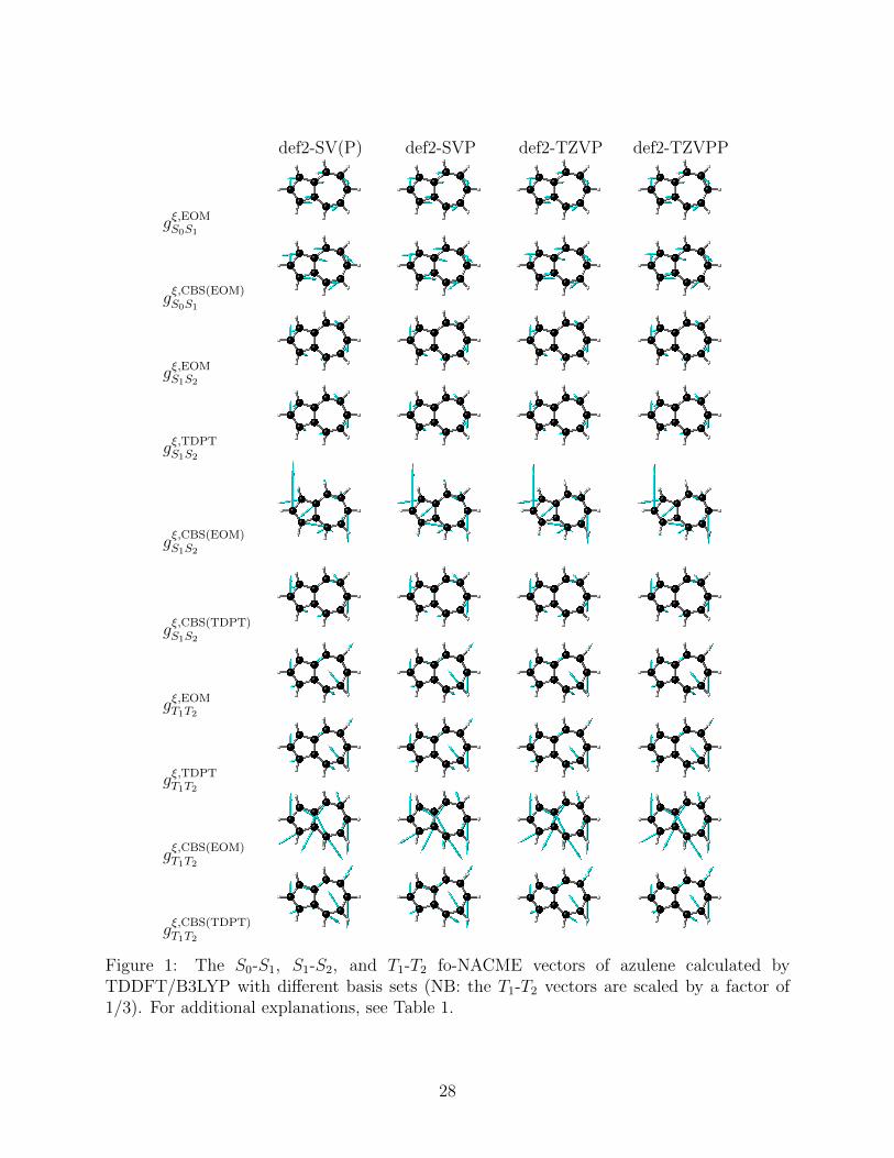
The first thing to note is the basis set convergence rates of the three methods. To

this end, the def2-SV(P), def2-SVP, def2-TZVP, and def2-TZVPP basis sets39 were used,

with the results documented in Table 1. As can be seen, the root-mean-square (RMS)

deviations of the EOM and TDPT fo-NACMEs from the near CBS results are smaller by 2

to 3 orders of magnitude than those by Eq. (11). Notably, while gξ,CBS(TDPT) approaches

slowly gξ,TDPT(def2-TZVPP) as the basis set is enlarged, gξ,CBS(EOM) does not approach

gξ,EOM(def2-TZVPP) and grossly overestimates the fo-NACMEs compared with both gξ,EOM

and gξ,TDPT (cf. Fig. 1). In fact, it can be proven13 that gξ,CBS(TDPT) (for ee fo-NACMEs)

coincides with gξ,TDPT, but gξ,CBS(EOM) in general does not agree with gξ,EOM in the CBS

limit. Therefore, from both numerical and theoretical points of view, gξ,CBS(EOM) should not

be recommended as a useful approach.

The overall accuracy of the calculated fo-NACME can be assessed by their use in com-

puting the IC rate constants (at T = 300 K) of S1 → S0, S2 → S1, and T2 → T1. The

MOMAP software package43–45 was used here, with Duschinsky rotation effects accounted

for. The harmonic vibrational frequencies were derived from the numerical Hessian yet based

on analytically evaluated TDDFT/B3LYP/def2-SVP gradients23 available in BDF. The re-

sults are collected in Table 2, to be compared with the experimental values (5.3 × 1011 s−1

for S1 → S027 and 3.5 × 108 s−1 for S2 → S1

28,29). It appears that all methods tend to

underestimate the IC rate constant of S1 → S0, which undergoes mainly through a con-

ical intersection.30 However, this cannot be fully ascribed to the quality of the calculated

fo-NACMEs, since the harmonic approximation for the vibrations also tends to underesti-

mate the rate constant of processes through conical intersections (CX). Such argument is

16

supported by the fact that the rate constant of the non-CX S2 → S1 is well reproduced by

both the EOM and TDPT based approaches. In contrast, both kCBS(TDPT)S2→S1

and especially

kCBS(EOM)S2→S1

are in large errors, showing again that the Hellmann-Feynman-like expression

(11) is unreliable. The T2 → T1 IC turns out to be orders of magnitude faster than both

S2 → S1 and S1 → S0, due to a much smaller energy gap (0.29, 1.34, and 1.59 eV for T2-T1,

S2-S1, and S1-S0, respectively). Because of this, the T2 → T1 IC cannot readily be detected

experimentally.

5 Conclusions and outlook

Different formulations of NAC-TDDFT for the fo-NACMEs between the ground and excited

states and between two excited states have been analyzed critically and demonstrated nu-

merically. The take-home messages include (1) the Hellmann-Feynman type of formulation

is hardly useful due to huge demands on basis sets; (2) the AWF-based formulation is not

theoretically founded and may give incorrect expressions; (3) the TDPT-based formulation

is most rigorous but the quadratic responses therein may be problematic, not because of

the formulation itself but due to the approximate nature of the exchange-correlation kernel;

(4) the EOM-based formulation is not only elegant but is also free of numerical instabili-

ties, and is therefore the recommended choice. Further extensions of the EOM variant of

NAC-TDDFT include (a) use of fragment localized molecular orbitals46–49 for efficient cal-

culations of large systems; (b) combination with spin adaptation23,50–52 for proper treatment

of open-shell systems; (c) combination with perturbative treatment of SOC,53–55 which is

another source for nonadiabatic couplings; and (d) combination with variational treatment of

SOC7,41,42,56–60 for systems containing very heavy elements. Progresses along these directions

are being made at our laboratory.

17

ACKNOWLEDGMENTS

This work was supported by the National Key R&D Program of China (Grant No. 2017YFB0203402),

National Natural Science Foundation of China (Grant Nos. 21833001 and 21973054), Moun-

tain Tai Climb Program of Shandong Province, and Key-Area Research and Development

Program of Guangdong Province (Grant No. 2020B0101350001).

BIOGRAPHICAL INFORMATION

Z. Wang was born in 1995 and obtained his Ph. D. in Chemistry from Peking Univer-

sity (2018). His research interests include spin-adapted open-shell time-dependent density

functional theory, fragmentation and semiempirical methods.

C. Wu was born in 1994 and obtained his Ph. D. in Chemistry from University of New

South Wales (2020). His research focuses on computer-aided rational design of organic dyes

and photocatalysts for polymerization.

W. Liu is Chair Professor at Shandong University, member of International Academy of

Quantum Molecular Science, fellow of Royal Society of Chemistry and Asia-Pacific Associ-

ation of Theoretical and Computational Chemists, recipient of Bessel Award of Humboldt

Foundation, Annual Medal of International Academy of Quantum Molecular Science, Pople

and Fukui Medals of Asia-Pacific Association of Theoretical and Computational Chemists.

His research interests include quantum electrodynamics, relativistic electronic structure the-

ory, many-body theory of strong correlation, time-dependent density functional theory, etc.

References

1 Cotton, S. J.; Liang, R.; Miller, W. H. On the adiabatic representation of Meyer-Miller

electronic-nuclear dynamics. J. Chem. Phys. 2017, 147, 064112.

2 Chernyak, V.; Mukamel, S. Density-matrix representation of nonadiabatic couplings in

18

time-dependent density functional (TDDFT) theories. J. Chem. Phys. 2000, 112, 3572–

3579.

3 Send, R.; Furche, F. First-order nonadiabatic couplings from time-dependent hybrid den-

sity functional response theory: Consistent formalism, implementation, and performance.

J. Chem. Phys. 2010, 132, 044107.

4 Lee, S.; Kim, E.; Lee, S.; Choi, C. H. Fast overlap evaluations for nonadiabatic molec-

ular dynamics simulations: Applications to SF-TDDFT and TDDFT. J. Chem. Theory

Comput. 2019, 15, 882–891.

5 Lee, S.; Horbatenko, Y.; Filatov, M.; Choi, C. H. Fast and Accurate Computation

of Nonadiabatic Coupling Matrix Elements Using the Truncated Leibniz Formula and

Mixed-Reference Spin-Flip Time-Dependent Density Functional Theory. J. Phys. Chem.

Lett. 2021, 12, 4722–4728.

6 Casida, M. E. In Recent Advances In Density Functional Methods: (Part I); Chang, D. P.,

Ed.; World Scientific: Singapore, 1995; pp 155–192.

7 Liu, W.; Xiao, Y. Relativistic time-dependent density functional theories. Chem. Soc.

Rev. 2018, 47, 4481–4509.

8 Tapavicza, E.; Tavernelli, I.; Rothlisberger, U. Trajectory Surface Hopping within Lin-

ear Response Time-Dependent Density-Functional Theory. Phys. Rev. Lett. 2007, 98,

023001.

9 Hu, C.; Hirai, H.; Sugino, O. Nonadiabatic couplings from time-dependent density func-

tional theory: Formulation in the Casida formalism and practical scheme within modified

linear response. J. Chem. Phys. 2007, 127, 064103.

10 Hu, C.; Sugino, O.; Hirai, H.; Tateyama, Y. Nonadiabatic couplings from the Kohn-

19

Sham derivative matrix: Formulation by time-dependent density-functional theory and

evaluation in the pseudopotential framework. Phys. Rev. A 2010, 82, 062508.

11 Tavernelli, I.; Curchod, B. F. E.; Laktionov, A.; Rothlisberger, U. Nonadiabatic cou-

pling vectors for excited states within time-dependent density functional theory in the

Tamm–Dancoff approximation and beyond. J. Chem. Phys. 2010, 133, 194104.

12 Alguire, E. C.; Ou, Q.; Subotnik, J. E. Calculating Derivative Couplings between Time-

Dependent Hartree–Fock Excited States with Pseudo-Wavefunctions. J. Phys. Chem. B

2015, 119, 7140–7149.

13 Li, Z.; Liu, W. First-order nonadiabatic coupling matrix elements between excited states:

A Lagrangian formulation at the CIS, RPA, TD-HF, and TD-DFT levels. J. Chem. Phys.

2014, 141, 014110.

14 Li, Z.; Suo, B.; Liu, W. First order nonadiabatic coupling matrix elements between

excited states: Implementation and application at the TD-DFT and pp-TDA levels. J.

Chem. Phys. 2014, 141, 244105.

15 Zhang, X.; Lu, G. First-order nonadiabatic couplings in extended systems by time-

dependent density functional theory. J. Chem. Phys. 2018, 149, 244103.

16 Ou, Q.; Bellchambers, G. D.; Furche, F.; Subotnik, J. E. First-order derivative couplings

between excited states from adiabatic TDDFT response theory. J. Chem. Phys. 2015,

142, 064114.

17 Zhang, X.; Herbert, J. M. Analytic derivative couplings in time-dependent density func-

tional theory: Quadratic response theory versus pseudo-wavefunction approach. J. Chem.

Phys. 2015, 142, 064109.

18 Rowe, D. J. Equations-of-Motion Method and the Extended Shell Model. Rev. Mod. Phys.

1968, 40, 153–166.

20

19 Etienne, T. Auxiliary many-body wavefunctions for TDDFRT electronic excited states:

Consequences for the representation of molecular electronic transitions. arXiv preprint

arXiv:2104.13616 2021,

20 Luzanov, A. V.; Zhikol, O. A. Electron invariants and excited state structural analysis

for electronic transitions within CIS, RPA, and TDDFT models. Int. J. Quantum Chem.

2010, 110, 902–924.

21 Olsen, J.; Jørgensen, P. Linear and nonlinear response functions for an exact state and

for an MCSCF state. J. Chem. Phys. 1985, 82, 3235–3264.

22 Parker, S. M.; Roy, S.; Furche, F. Unphysical divergences in response theory. J. Chem.

Phys. 2016, 145, 134105.

23 Wang, Z.; Li, Z.; Zhang, Y.; Liu, W. Analytic energy gradients of spin-adapted open-shell

time-dependent density functional theory. J. Chem. Phys. 2020, 153, 164109.

24 Fatehi, S.; Alguire, E.; Shao, Y.; Subotnik, J. E. Analytic derivative couplings between

configuration-interaction-singles states with built-in electron-translation factors for trans-

lational invariance. J. Chem. Phys. 2011, 135, 234105.

25 Furche, F.; Ahlrichs, R. Adiabatic time-dependent density functional methods for excited

state properties. J. Chem. Phys. 2002, 117, 7433–7447.

26 Furche, F.; Ahlrichs, R. Erratum: “Time-dependent density functional methods for ex-

cited state properties” [J. Chem. Phys. 117, 7433 (2002)]. J. Chem. Phys. 2004, 121,

12772–12773.

27 Ippen, E. P.; Shank, C. V.; Woerner, R. L. Picosecond dynamics of azulene. Chem. Phys.

Lett. 1977, 46, 20–23.

28 Hirata, Y.; Lim, E. C. Radiationless transitions in azulene: Evidence for the ultrafast

S2→S0 internal conversion. J. Chem. Phys. 1978, 69, 3292–3296.

21

29 Wagner, B. D.; Tittelbach-Helmrich, D.; Steer, R. P. Radiationless decay of the S2 states

of azulene and related compounds: solvent dependence and the energy gap law. J. Phys.

Chem. 1992, 96, 7904–7908.

30 Amatatsu, Y.; Komura, Y. Reaction coordinate analysis of the S1-S0 internal conversion

of azulene. J. Chem. Phys. 2006, 125, 174311.

31 Beer, M.; Longuet-Higgins, H. C. Anomalous Light Emission of Azulene. J. Chem. Phys.

1955, 23, 1390–1391.

32 Liu, W.; Hong, G.; Dai, D.; Li, L.; Dolg, M. The Beijing 4-component density functional

theory program package (BDF) and its application to EuO, EuS, YbO and YbS. Theor.

Chem. Acc. 1997, 96, 75–83.

33 Liu, W.; Wang, F.; Li, L. The Beijing Density Functional (BDF) program package:

Methodologies and applications. J. Theor. Comput. Chem. 2003, 2, 257–272.

34 Liu, W.; Wang, F.; Li, L. In Recent Advances in Relativistic Molecular Theory ; Hirao, K.,

Ishikawa, Y., Eds.; World Scientific: Singapore, 2004; pp 257–282.

35 Liu, W.; Wang, F.; Li, L. In Encyclopedia of Computational Chemistry ; von

Rague Schleyer, P., Allinger, N. L., Clark, T., Gasteiger, J., Kollman, P. A., Schae-

fer III, H. F., Eds.; Wiley: Chichester, UK, 2004.

36 Zhang, Y. et al. BDF: A relativistic electronic structure program package. J. Chem. Phys.

2020, 152, 064113.

37 Becke, A. D. Density-functional thermochemistry. III. The role of exact exchange. J.

Chem. Phys. 1993, 98, 5648.

38 Stephens, P. J.; Devlin, F. J.; Chabalowski, C. F.; Frisch, M. J. AB-INITIO CALCULA-

TION OF VIBRATIONAL ABSORPTION AND CIRCULAR-DICHROISM SPECTRA

USING DENSITY-FUNCTIONAL FORCE-FIELDS. J. Phys. Chem. 1994, 98, 11623.

22

39 Weigend, F.; Ahlrichs, R. Balanced basis sets of split valence, triple zeta valence and

quadruple zeta valence quality for H to Rn: Design and assessment of accuracy. Phys.

Chem. Chem. Phys. 2005, 7, 3297–3305.

40 Wang, F.; Liu, W. Comparison of Different Polarization Schemes in Open-shell Relativis-

tic Density Functional Calculations. J. Chin. Chem. Soc. (Taipei) 2003, 50, 597–606.

41 Gao, J.; Liu, W.; Song, B.; Liu, C. Time-dependent four-component relativistic density

functional theory for excitation energies. J. Chem. Phys. 2004, 121, 6658–6666.

42 Gao, J.; Zou, W.; Liu, W.; Xiao, Y.; Peng, D.; Song, B.; Liu, C. Time-dependent four-

component relativistic density-functional theory for excitation energies. II. The exchange-

correlation kernel. J. Chem. Phys. 2005, 123, 054102.

43 Niu, Y.; Li, W.; Peng, Q.; Geng, H.; Yi, Y.; Wang, L.; Nan, G.; Wang, D.; Shuai, Z.

MOlecular MAterials Property Prediction Package (MOMAP) 1.0: a software package

for predicting the luminescent properties and mobility of organic functional materials.

Mol. Phys. 2018, 116, 1078–1090.

44 Peng, Q.; Yi, Y.; Shuai, Z.; Shao, J. Excited state radiationless decay process with

Duschinsky rotation effect: Formalism and implementation. J. Chem. Phys. 2007, 126,

114302.

45 Niu, Y.; Peng, Q.; Shuai, Z. Promoting-mode free formalism for excited state radiationless

decay process with Duschinsky rotation effect. Sci. China Ser. B: Chem. 2008, 51, 1153–

1158.

46 Wu, F.; Liu, W.; Zhang, Y.; Li, Z. Linear-Scaling Time-Dependent Density Functional

Theory Based on the Idea of “From Fragments to Molecule”. J. Chem. Theory Comput.

2011, 7, 3643–3660.

23

47 Liu, J.; Zhang, Y.; Liu, W. Photoexcitation of Light-Harvesting C–P–C60 Triads: A

FLMO-TD-DFT Study. J. Chem. Theory Comput. 2014, 10, 2436–2448.

48 Li, Z.; Li, H.; Suo, B.; Liu, W. Localization of Molecular Orbitals: From Fragments to

Molecule. Acc. Chem. Res. 2014, 47, 2758–2767.

49 Li, H.; Liu, W.; Suo, B. Localization of open-shell molecular orbitals via least change

from fragments to molecule. J. Chem. Phys. 2017, 146, 104104.

50 Li, Z.; Liu, W. Spin-adapted open-shell random phase approximation and time-dependent

density functional theory. I. Theory. J. Chem. Phys. 2010, 133, 064106.

51 Li, Z.; Liu, W.; Zhang, Y.; Suo, B. Spin-adapted open-shell time-dependent density

functional theory. II. Theory and pilot application. J. Chem. Phys. 2011, 134, 134101.

52 Li, Z.; Liu, W. Spin-adapted open-shell time-dependent density functional theory. III. An

even better and simpler formulation. J. Chem. Phys. 2011, 135, 194106, (E)138, 029904

(2013).

53 Li, Z.; Xiao, Y.; Liu, W. On the spin separation of algebraic two-component relativistic

Hamiltonians. J. Chem. Phys. 2012, 137, 154114.

54 Li, Z.; Xiao, Y.; Liu, W. On the spin separation of algebraic two-component relativistic

Hamiltonians: Molecular properties. J. Chem. Phys. 2014, 141, 054111.

55 Li, Z.; Suo, B.; Zhang, Y.; Xiao, Y.; Liu, W. Combining spin-adapted open-shell TD-DFT

with spin-orbit coupling. Mol. Phys. 2013, 111, 3741–3755.

56 Peng, D.; Zou, W.; Liu, W. Time-dependent quasirelativistic density-functional theory

based on the zeroth-order regular approximation. J. Chem. Phys. 2005, 123, 144101.

57 Xu, W.; Zhang, Y.; Liu, W. Time-dependent relativistic density functional study of Yb

and YbO. Sci. China Ser. B: Chem. 2009, 52, 1945–1953.

24

58 Xu, W.; Ma, J.; Peng, D.; Zou, W.; Liu, W.; Staemmler, V. Excited states of ReO4-: A

comprehensive time-dependent relativistic density functional theory study. Chem. Phys.

2009, 356, 219–228.

59 Zhang, Y.; Xu, W.; Sun, Q.; Zou, W.; Liu, W. Excited states of OsO4: A comprehensive

time-dependent relativistic density functional theory study. J. Comput. Chem. 2010, 31,

532–551.

60 Liu, W. Essentials of relativistic quantum chemistry. J. Chem. Phys. 2020, 152, 180901.

25

Table 1: Root-mean-square deviations of TDDFT/B3LYP fo-NACMEs (in Bohr−1) be-tween different states of azulene from the reference data: gξ,EOM(def2-TZVPP) for gξ,EOM

and gξ,CBS(EOM), and gξ,TDPT(def2-TZVPP) for gξ,TDPT and gξ,CBS(TDPT). gξ,EOM by Eq.(42)/(43); gξ,TDPT by Eq. (42)/(56); gξ,CBS(EOM) by Eq. (11) with γIJ (38); gξ,CBS(TDPT) byEq. (11) with γIJ (57).

def2-SV(P) def2-SVP def2-TZVP def2-TZVPP

gξ,EOMS0S1

0.0037 0.0006 0.0002 0.0000

gξ,CBS(EOM)S0S1

0.1077 0.1072 0.0601 0.0585

gξ,EOMS1S2

0.0028 0.0031 0.0003 0.0000

gξ,TDPTS1S2

0.0037 0.0042 0.0003 0.0000

gξ,CBS(EOM)S1S2

0.4774 0.4746 0.4949 0.4941

gξ,CBS(TDPT)S1S2

0.0865 0.0841 0.0523 0.0505

gξ,EOMT1T2

0.0726 0.0775 0.0039 0.0000

gξ,TDPTT1T2

0.0724 0.0774 0.0039 0.0000

gξ,CBS(EOM)T1T2

1.5479 1.5688 1.4715 1.4685

gξ,CBS(TDPT)T1T2

0.4406 0.4356 0.2514 0.2419

26

Table 2: TDDFT/B3LYP internal conversion rate constants (k in s−1) between differentstates of azulene. The experimental values are 5.3× 1011 s−1 for kS1→S0

27 and 3.5× 108 s−1

for kS2→S1 .28,29 For additional explanations, see Table 1.

def2-SV(P) def2-SVP def2-TZVP def2-TZVPPkEOMS1→S0

7.96E+08 8.00E+08 7.67E+08 7.68E+08

kCBS(EOM)S1→S0

1.27E+09 1.32E+09 1.05E+09 1.04E+09kEOMS2→S1

1.29E+09 1.27E+09 1.25E+09 1.25E+09kTDPTS2→S1

1.38E+09 1.36E+09 1.35E+09 1.34E+09

kCBS(EOM)S2→S1

1.25E+10 1.26E+10 1.31E+10 1.31E+10

kCBS(TDPT)S2→S1

2.25E+09 2.44E+09 1.96E+09 1.94E+09kEOMT2→T1 1.40E+13 1.42E+13 1.23E+13 1.22E+13kTDPTT2→T1 1.39E+13 1.41E+13 1.22E+13 1.21E+13

kCBS(EOM)T2→T1 8.75E+13 8.92E+13 8.14E+13 8.11E+13

kCBS(TDPT)T2→T1 2.33E+13 2.33E+13 1.78E+13 1.74E+13

27

def2-SV(P) def2-SVP def2-TZVP def2-TZVPP

gξ,EOMS0S1

gξ,CBS(EOM)S0S1

gξ,EOMS1S2

gξ,TDPTS1S2

gξ,CBS(EOM)S1S2

gξ,CBS(TDPT)S1S2

gξ,EOMT1T2

gξ,TDPTT1T2

gξ,CBS(EOM)T1T2

gξ,CBS(TDPT)T1T2

Figure 1: The S0-S1, S1-S2, and T1-T2 fo-NACME vectors of azulene calculated byTDDFT/B3LYP with different basis sets (NB: the T1-T2 vectors are scaled by a factor of1/3). For additional explanations, see Table 1.

28