N R I NODE-SPECIFIC INFORMATION

Under review as a conference paper at ICLR 2022

NEURAL RELATIONAL INFERENCE WITHNODE-SPECIFIC INFORMATION

Anonymous authorsPaper under double-blind review

ABSTRACT

Inferring interactions among entities is an important problem in studying dynamicalsystems, which greatly impacts the performance of downstream tasks, such asprediction. In this paper, we tackle this problem in a setting where each entitycan potentially have a set of individualized information that other entities cannothave access to. Specifically, we represent the system using a graph in which theindividualized information become node-specific information (NSI). We build ourmodel in the framework of Neural Relation Inference (NRI), where the interactionamong entities are interpretably uncovered using variational inference. We adoptNRI model to incorporate the individualized information by introducing privatenodes in the graph that represent NSI. Such representation enables us to uncovermore accurate relations among the agents and therefore leads to better performanceon the downstream tasks. Our experiment results over real-world datasets validatethe merit of our proposed algorithm.

1 INTRODUCTION

Our world includes many different types of systems that involve multiple entities interacting with eachother, from biology to sports, from social media to driving situations. Modelling the behaviour of suchdynamical systems is a challenging task, which requires uncovering different types of interactionsamong the entities and how they affect each other.

Recent approaches in machine learning learn the interactions among the entities through graph-basedmodels and attention-based models, in which the representation of an entity is updated throughits relationship with other entities. Such relationships are usually either pre-defined or uncoveredby learning. Kipf et al, in Kipf et al. (2018), proposed neural relational inference (NRI). NRI hasan encoder-decoder structure in the framework of variational inference (Kingma & Welling, 2013;Rezende et al., 2014) in which the latent codes represent different types of interactions among theentities. The distributions over the latent variables are inferred based on the input features of theentities and a graph structure is formed by sampling from these distributions. The decoder of themodel is a GNN-based algorithm that runs over the uncovered graph to update the features of entities.The model shows prominent performance over many synthetic and real-world datasets.

Uncovering the interaction among entities in NRI and other models in the GNN literature is studied inproblems where the features of the entities are completely observable and the GNN-based algorithmis also run on the observable features. However, in many real-world problems there is a set of hiddenfeatures that affect the way entities interact with each other. For example consider the problem ofpredicting the future position of vehicles in a driving scenario. In order to uncover the relation ofa target vehicle with other vehicles not only should we consider the features extracted from theobservations from vehicles, e.g. their trajectories up to current time, but also we should take intoaccount the intention of the target vehicle. In fact, intention, which can be an immediate action ora longer term goal, forms a set of features that is only accessible by the target vehicle and othervehicle cannot know it. In this paper we call such feature the Node-Specific Information (NSI) orindividualized features. Formally, NSI is a set of features that is only accessible by one node in agraph structure but affects the interactions of that node with other nodes. Our goal is to efficientlyexploit NSI to build more accurate graph structures and consequently achieve better performance inthe downstream tasks. Towards this goal, the first step is to find a proper representation for NSI in ourgraph structure. We propose introducing a new set of nodes in the graph that carry NSI and call them

1


private nodes. Observable features of the entities are then denoted by public nodes. Therefore eachentity can be represented by a public and private node. We introduce our model in the frameworkof NRI, i.e. a variational inference model that uncovers different types of interaction among theentities. We carefully design the encoder and decoder part of our model to ensure that NSI remainsan individual feature for one entity and does not affect the interaction modelling of the other entities.At the same time, through experiment we show that such modelling of NSI is very efficient and canresult in significant improvement on the performance on downstream tasks. The main contributionsof this work are the followings:

• To the best of our knowledge the problem of having individualized information for eachentity has not been previously studied in the framework of relational learning. We tacklethis problem by introducing a new set of nodes in a graph structure that represents theindividualized information. These nodes are used during the process of relational inferenceas well as performing the downstream task, i.e. trajectory prediction in our case.

• We show that our proposed model can exploit NSI efficiently by introducing minimumadditional computational complexity compared to the original NRI model and its variants.

• The results of our experiments on real-world datasets show that our model can outperformour baseline and achieve the state-of-the-art results on the defined tasks.

2 RELATED WORK

Interaction modelling: Relational learning is a popular approach for the problems with dependencystructure among the data points. Such dependency can be given in some domains. But in manydomains it has to be learned. For example approaches like locally linear embedding (LLE) (Roweis &Saul, 2000) and Isomap (Tenenbaum et al., 2000) use kNN for forming such relationships based ondifferent measures of similarities among the data points. More recently, neural networks have becomethe dominant tools for learning this dependencies based on different architectures and paradigms(Kipf & Welling, 2017; Hamilton et al., 2017; Garcia Duran & Niepert, 2017; Monti et al., 2017;Velickovic et al., 2017; Franceschi et al., 2019).

The most relevant works to our proposed model are NRI (Kipf et al., 2018) and dynamic NRI (dNRI)(Graber & Schwing, 2020), which are discussed in more details in the next section. Recently, Li et al.(2020) introduced similar ideas for multi-modal trajectories prediction. Extensions of NRI in otherdirections than ours also appeared in the literature. For example, Li et al. (2019) tries to uncoverinteractions by imposing some structural constraints on the prior and Webb et al. (2019) introducesthe idea of factorized graph for NRI.

The other common approach for uncovering relationships among the entities is based on the idea ofattention. This idea has been used in Narasimhan et al. (2018); Hoshen (2017); Van Steenkiste et al.(2017); Garcia & Bruna (2017); Monti et al. (2017); Velickovic et al. (2017), where the attentionmechanism is the main tool for interaction uncovering, however, it is also used as a building block forGNNs.

Future trajectory prediction as evaluation metric: We define our problem as uncovering theinteractions of entities in a multi-agent dynamical system, where the evaluation is based on theaccuracy of future trajectory prediction. Trajectory prediction is in fact an important problem in manymulti-agent systems, including the ever growing area of autonomous driving. In fact, our approachfalls into the category of multivariate time-series prediction (Yu et al., 2018; Wu et al., 2019; Senet al., 2019; Salinas et al., 2020; Rangapuram et al., 2018; Li et al., 2018; Bai et al., 2018), in whichthe prediction is based on the relationship among the series. Specifically we use the relationshipof the entities in the GNNs framework. GNN has been widely used in the trajectory prediction,especially in the application of autonomous driving and significantly improved the performance inthis area. For example, Salzmann et al. (2020) uses GNN to capture the relationship among differentroad users (vehicles and pedestrian), Gao et al. (2020) uses graph attention networks (GATs) to learnthe relationship among agents and different components of map data, and Liang et al. (2020) usesgraph convolutional networks (GCNs) to learn the interaction among lanes and vehicles.

In our experiment we consider the scenarios in which the goal (final) position of the entities is givenas the individualized information. In the context of goal-aware prediction, there have been someeffort in the area of autonomous driving that are not based on explicit relational learning (Rhinehart

2


et al., 2019; 2018). In these papers, the prediction is based on an autoregressive flow-based modelthat considers a collective observation of all entities to make prediction for each of them.

3 BACKGROUND: NEURAL RELATIONAL INFERENCE (NRI)

NRI is an unsupervised model that learns to infer the interaction types among entities in a multi-agentsystems in order to model the dynamics of the system. The model is defined as the problem ofpredicting the future trajectory of entities given the past trajectories. Formally, the trajectories ofN entities are given for T time steps. Entity i is denoted by xi = (x1

i ,x2i , ...,x

Ti ). The set of all

trajectories at time t is denoted by xt = {xt1,xt2, ...,xtN} and x = (x1,x2, ...,xT ) denotes thewhole trajectories for all agents. NRI tries to model the system by maximizing the log-likelihood ofthe observations, log p(x), in the framework of variational inference, i.e. maximizes the evidencelower-bound (ELBO):

L(θ, φ) = Eqφ(z|x)[log pθ(x|z)]− KL[qφ(z|x)||p(z)

], (1)

where latent variable z has a categorical distribution and represents the interaction among entities.More specifically, zij is a K-dimensional vector that denotes the type interaction between entitiesxi and xj . The entities in the NRI model are represented using nodes of a graph1 and therefore theinteractions are directed edges on this graph. Parameters of p(.) and q(.) models are denoted by θand φ, respectively. The three probability distributions in Eq. 1 are:

• The variational posterior, qφ(z|x), is implemented using amortized inference parameter-ized by a neural network, namely the encoder network. Given the input trajectories, theencoder network predicts the type of edges on the graph. The latent variable z is assumedto have a categorical distribution. Samples from this distribution form the edges of thegraph. In order to backpropagate the error signals to the encoder layers, we need to makethe sampling process differentiable. In NRI this is done by approximating the posteriordistribution and reparamterezation of Gumble distribution (Jang et al., 2017; Maddison et al.,2017):

zij = softmax((h2(i,j) + g)/τ) (2)

where h2(i,j) is the last output of the encoder before the softmax layer and g ∈ RK shows i.i.d.

samples drawn from Gumbel(0, 1) and τ is a hyperparameter that controls the smoothnessof the distribution.

• The prior, p(z) =∏i 6=j p(zij), is assumed to be a factorized uniform categorical distribu-

tion over the edges.

• The likelihood, pθ(x|z), is implemented by the decoder network and predicts the futuretrajectories given the uncovered structure of the graph.

The prediction in NRI is done in an autoregressive fashion. However, the ground truth trajectory isfed to the model for few steps during the training to improve the performance of the decoder (teacherforcing). NRI is its original form has two main shortcomings:

1. The latent variable z, which defines the edge types, is fixed for the whole prediction horizon.That is, the model uncovers the interaction among the agents at the beginning and assumesthe interactions are unchanged over the next time steps. This is not necessary is validassumption as the agents can dynamically change their interactions in the system.

2. The prior distribution is assumed to be uniform and not conditioned on the previous observa-tions. Both of these assumptions can hurt the performance of the model in longer predictionhorizons since samples from the prior provides minimum information about the input.

More recently, Graber & Schwing (2020) pointed out the above issues and addressed them in dynamicneural relation inference (dNRI) model. The prior distribution of in dNRI is conditional and defined

1Throughout the paper, entities and nodes as well as interactions and edges are used interchangeably, basedon the context.

3


as:

p(z|x) :=T∏t=1

p(zt|x1:t, z1:t−1), (3)

which is implemented by another set of MLP and LSTM layers that form the encoder of the pθ(.)model. The experiments show that, by resolving those issues, dNRI achieves better predictionperformance than NRI.

4 MODEL DESCRIPTION

4.1 PROBLEM STATEMENT

We define our problem in the setting of NRI. However, we assume that, in addition to the observablefeature set x, each entity i can potentially have access to a set of individualized features cti at eachtime step t. cti cannot be observed by other entities, however its effect might be observed in thefuture times steps through xt+ki (k > 0). Similar to the observable features, we denote the set ofindividualized features for each agent by ci = (c1i , c

2i , ..., c

Ti ), set of individualized features for all

agents at time t by ct = {ct1, ct2, ..., ctN}, and set of all individualized features by c = (c1, c2, ..., cT ).We still study the problem of modelling the dynamics of the system through predicting the futuretrajectories of the entities. However, we aim to exploit the individualized features in a way that theinteraction among the entities are inferred more accurately and, therefore, provide a better model forthe underlying dynamics of the system, which can lead to better prediction performance.

4.2 REPRESENTATION OF INDIVIDUALIZED FEATURES IN THE GRAPH: PRIVATE VS PUBLICNODES

Entity 1

Figure 1: Blue dots and black dots show thepublic and private nodes, respectively. Dif-ferent type of interactions among entities aredepicted as directed edges among the nodeswith different colors.

In order to build the interaction inference model, we needto first represent the individualized features in the graph.Note that simply augmenting the observation features xiwith the individualized features and building a new set offeatures, e.g. yi = f(xi, ci), is not a solution here, as thiswill affect the interaction uncovering among the agents,which is in contrary with our initial assumption about theaccessibility of individualized features.

Here, we propose adding a new set of nodes to representthe individualized features and we call these nodes pri-vate nodes. We also refer to the nodes that represent theobservable nodes as public nodes for clarification. There-fore each entity i at each time t can be shown using apublic node and private node corresponding to xti and cti,respectively. A private node is only accessible by its cor-responding public node while a public node is accessibleby all other public nodes. Interaction among public nodes and their corresponding private node isalways fixed, while interaction among public nodes are learned. Fig. 1 shows the uncovered graph ofan example system at time step t. Note that there is always an edge between the public node and itscorresponding private node, which is shown in black in the figure. This edge represents all types ofinteractions. Representing the individualized features using the private nodes allows us to employ aunified framework to uncover the graph, without creating a computational overhead.

4.3 MODEL COMPONENTS

In order to learn the interactions in our model we maximize the ELBO of the following form:

LNRI-NSI(θ, φ) = Eqφ(z|x,c)[log pθ(x|z, c)]− KL[qφ(z|x, c)||pθ(z|x, c)

]. (4)

The conditional probability distributions are parameterized by neural networks and factorzied as:

4


Unshared encoder

Unshared encoder

GNN (shared encoder)Public node

encoding

Private node encoding

Sample

soft

max

Bi-LSTM

LSTM

soft

max

Uncovered graph with all edge types

Con

cat

GNN per edge type

Multi-head graph encoding

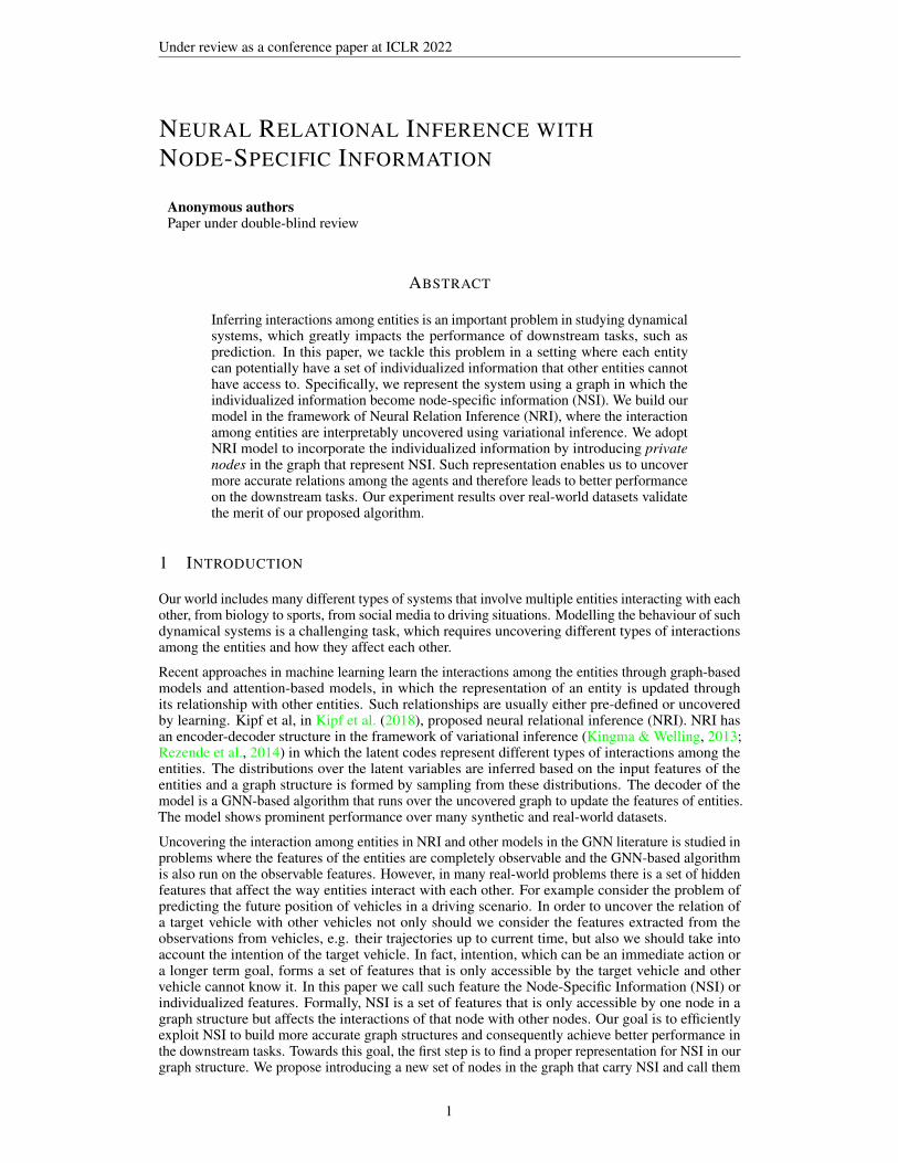
Figure 2: Proposed model. Encoded observable and individualized features are fed to GNN model to updatethe node features. The output of the GNN is fed to both pθ(.) and qφ(.) encoders to provide the uncoveredinteractions among the agents. The parameter of pθ(.) and qφ(.) distributions are learned to minimize theirKL divergence. Moreover, during the training the edges are randomly drawn from the pθ(.) encoder to betteroptimize the parameters of this model. The sampled edges together with the input features are fed to the decodermodel to output the prediction at each time step.

qφ(z|x, c) =T∏t=1

qφ(zt|x1:T , z1:t−1, c1:T ) =

N∏i=1

N∏j=1j 6=i

T∏t=1

qφ(ztij |x1:T , z1:t−1, c1:Tj ), (5)

pθ(z|x, c) =T∏t=1

pθ(zt|x1:t, z1:t−1, c1:t) =

N∏i=1

N∏j=1j 6=i

T∏t=1

pθ(ztij |x1:t, z1:t−1, c1:tj ), (6)

pθ(x|z, c) =T∏t=1

pθ(xt+1|x1:t, zt, c1:t) =

N∏j=1

T∏t=1

pθ(xt+1j |x

1:t, zt, c1:tj ). (7)

Note that at each time step, the edge uncovering and prediction for each public node depend only onits own private node. Here we describe the details of each component.

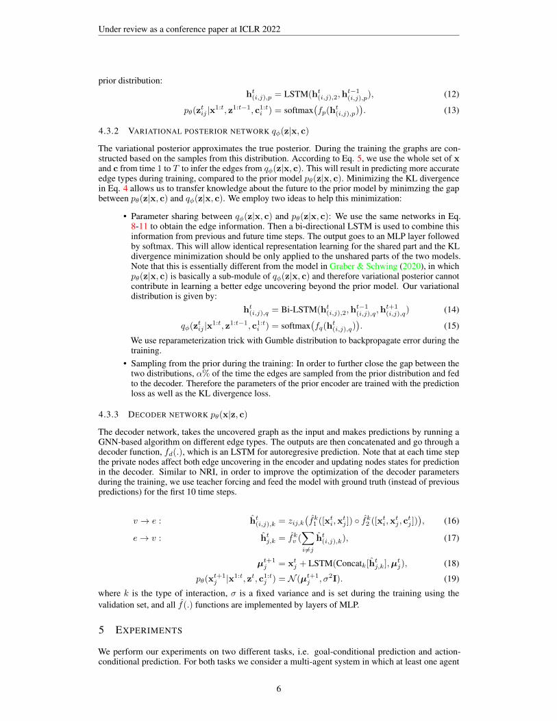
4.3.1 CONDITIONAL PRIOR NETWORK pθ(z|x, c)

The prior distribution forms the different types of interactions given the past and current status ofpublic and private nodes at each time step using the autoregressive model in Eq. 6. We use a GNNarchitecture for message passing where the graph is fully-connected for the set of public nodes andfor the private nodes there is only an edge towards their corresponding public node.

node embedding: mtj = fxemb(x

tj) , ntj = fcemb(c

tj), (8)

v → e : ht(i,j),1 = f1e ([mti,m

tj ]), (9)

e→ v : htj = f1v (∑i 6=j

ht(i,j),1), (10)

v → e : ht(i,j),2 = f2e ([hti,h

tj ]) ◦ f3e ([hti,htj ,ntj ]), (11)

where ◦ denotes Hadamard product and v and e represent nodes and edges of the graph, respectively.Note that using our proposed represenetation, we can handle the general setting in which not allentities necessarily have individualized features. In the case that these features are not provided foran entity, f3e (.) is masked out and replaced by an all one vector. By using two levels of messagepassing we make sure that all observable nodes are considered to infer an edge. In the first level onlythe observable features are used so that the final relationship uncovering for each entity is not affectedby other entities’ individualized features. We use multilayer perceptron (MLP) layers for all of thef(.) functions. In order to take into account the previous interactions, the embedding ht(i,j),2 at eachtime step is fed to layers of LSTM followed by MLP and softmax to output the actual conditional

5


prior distribution:ht(i,j),p = LSTM(ht(i,j),2,h

t−1(i,j),p), (12)

pθ(ztij |x1:t, z1:t−1, c1:ti ) = softmax

(fp(h

t(i,j),p)

). (13)

4.3.2 VARIATIONAL POSTERIOR NETWORK qφ(z|x, c)

The variational posterior approximates the true posterior. During the training the graphs are con-structed based on the samples from this distribution. According to Eq. 5, we use the whole set of xand c from time 1 to T to infer the edges from qφ(z|x, c). This will result in predicting more accurateedge types during training, compared to the prior model pθ(z|x, c). Minimizing the KL divergencein Eq. 4 allows us to transfer knowledge about the future to the prior model by minimzing the gapbetween pθ(z|x, c) and qφ(z|x, c). We employ two ideas to help this minimization:

• Parameter sharing between qφ(z|x, c) and pθ(z|x, c): We use the same networks in Eq.8-11 to obtain the edge information. Then a bi-directional LSTM is used to combine thisinformation from previous and future time steps. The output goes to an MLP layer followedby softmax. This will allow identical representation learning for the shared part and the KLdivergence minimization should be only applied to the unshared parts of the two models.Note that this is essentially different from the model in Graber & Schwing (2020), in whichpθ(z|x, c) is basically a sub-module of qφ(z|x, c) and therefore variational posterior cannotcontribute in learning a better edge uncovering beyond the prior model. Our variationaldistribution is given by:

ht(i,j),q = Bi-LSTM(ht(i,j),2,ht−1(i,j),q,h

t+1(i,j),q) (14)

qφ(ztij |x1:t, z1:t−1, c1:ti ) = softmax

(fq(h

t(i,j),q)

). (15)

We use reparameterization trick with Gumble distribution to backpropagate error during thetraining.

• Sampling from the prior during the training: In order to further close the gap between thetwo distributions, α% of the time the edges are sampled from the prior distribution and fedto the decoder. Therefore the parameters of the prior encoder are trained with the predictionloss as well as the KL divergence loss.

4.3.3 DECODER NETWORK pθ(x|z, c)

The decoder network, takes the uncovered graph as the input and makes predictions by running aGNN-based algorithm on different edge types. The outputs are then concatenated and go through adecoder function, fd(.), which is an LSTM for autoregresive prediction. Note that at each time stepthe private nodes affect both edge uncovering in the encoder and updating nodes states for predictionin the decoder. Similar to NRI, in order to improve the optimization of the decoder parametersduring the training, we use teacher forcing and feed the model with ground truth (instead of previouspredictions) for the first 10 time steps.

v → e : ht(i,j),k = zij,k(fk1 ([x

ti,x

tj ]) ◦ fk2 ([xti,xtj , ctj ])

), (16)

e→ v : htj,k = fkv (∑i 6=j

ht(i,j),k), (17)

µt+1j = xtj + LSTM(Concatk[htj,k],µ

tj), (18)

pθ(xt+1j |x

1:t, zt, c1:tj ) = N (µt+1j , σ2I). (19)

where k is the type of interaction, σ is a fixed variance and is set during the training using thevalidation set, and all f(.) functions are implemented by layers of MLP.

5 EXPERIMENTS

We perform our experiments on two different tasks, i.e. goal-conditional prediction and action-conditional prediction. For both tasks we consider a multi-agent system in which at least one agent

6


has access to its individualized features. Both of these tasks are of great interest in the contextof trajectory prediction, with important downstream applications such as planning. For the goal-conditional task the individualized feature is the final goal (position) of the agent. Therefore, thisinformation is fixed for the whole prediction horizon or at least for multiple time steps, ct:t+li = gti forl > 1. For the action-conditional task the individualized feature is the next action of the agent, whichchanges at every time step, cti = uti. We refer to our model as NRI-NSI. In all of our experiment weuse ADAM optimizer (Kingma & Ba, 2015) with learning rate 0.0001.

Metrics: Since our final task is trajectory prediction of the entities, we use minimum averagedisplacement error (minADE) and minimum final displacement error (FDE) as the evaluation metrics.ADE: average mean square error (MSE) over all time steps between the ground truth future trajectoryand the predicted trajectory. FDE: MSE between the final ground truth position and the predictedfinal position. Note that since we are using a stochastic model in the decoder, the minADE andminFDE are the closest sample to the ground truth over 20 different sampled predictions. We followthis scheme for all of the baselines, too.

Baselines: For both action-conditional and goal-conditional prediction, we compare our model withNRI and dNRI where the individualized features are fed to the model at the last stage of decoder foreach of the entities, i.e. before outputting the distribution of the predictions.

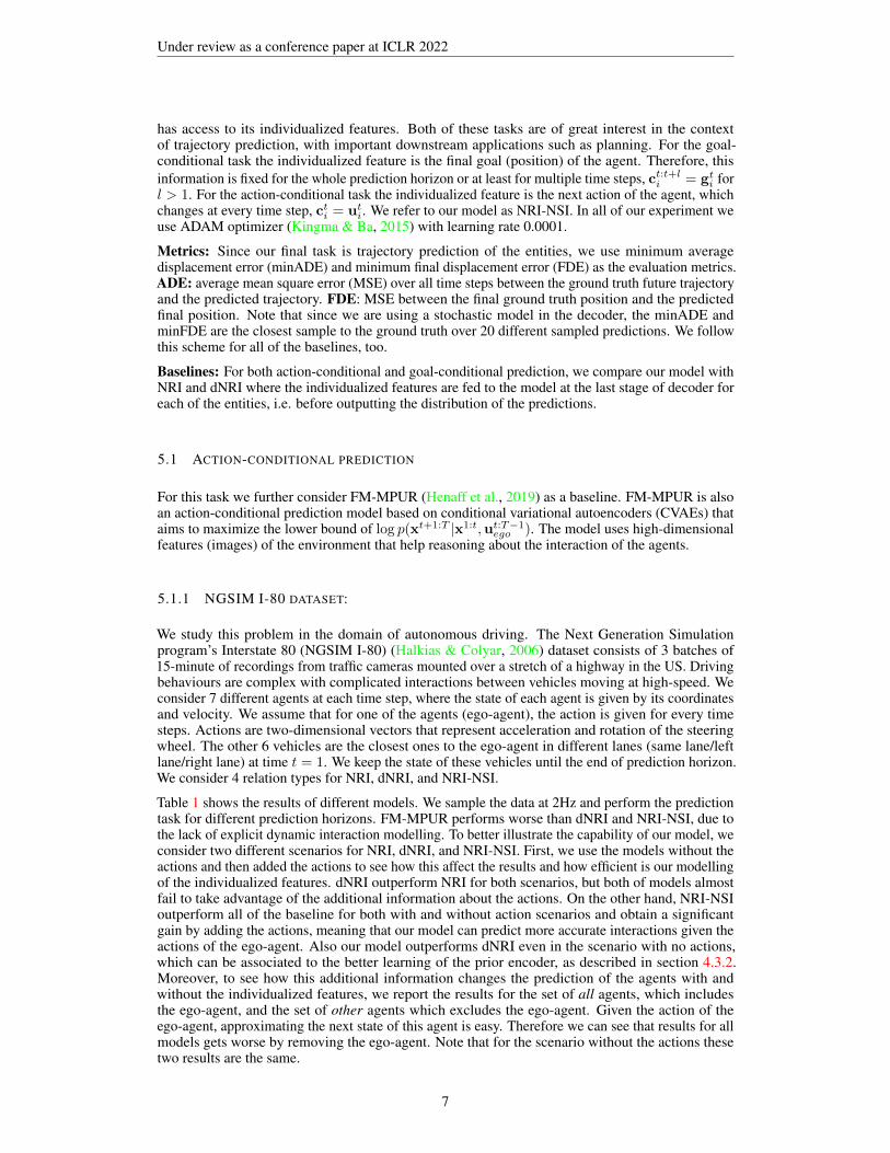
5.1 ACTION-CONDITIONAL PREDICTION

For this task we further consider FM-MPUR (Henaff et al., 2019) as a baseline. FM-MPUR is alsoan action-conditional prediction model based on conditional variational autoencoders (CVAEs) thataims to maximize the lower bound of log p(xt+1:T |x1:t,ut:T−1ego ). The model uses high-dimensionalfeatures (images) of the environment that help reasoning about the interaction of the agents.

5.1.1 NGSIM I-80 DATASET:

We study this problem in the domain of autonomous driving. The Next Generation Simulationprogram’s Interstate 80 (NGSIM I-80) (Halkias & Colyar, 2006) dataset consists of 3 batches of15-minute of recordings from traffic cameras mounted over a stretch of a highway in the US. Drivingbehaviours are complex with complicated interactions between vehicles moving at high-speed. Weconsider 7 different agents at each time step, where the state of each agent is given by its coordinatesand velocity. We assume that for one of the agents (ego-agent), the action is given for every timesteps. Actions are two-dimensional vectors that represent acceleration and rotation of the steeringwheel. The other 6 vehicles are the closest ones to the ego-agent in different lanes (same lane/leftlane/right lane) at time t = 1. We keep the state of these vehicles until the end of prediction horizon.We consider 4 relation types for NRI, dNRI, and NRI-NSI.

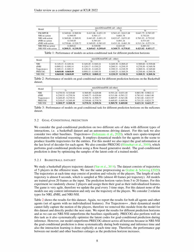
Table 1 shows the results of different models. We sample the data at 2Hz and perform the predictiontask for different prediction horizons. FM-MPUR performs worse than dNRI and NRI-NSI, due tothe lack of explicit dynamic interaction modelling. To better illustrate the capability of our model, weconsider two different scenarios for NRI, dNRI, and NRI-NSI. First, we use the models without theactions and then added the actions to see how this affect the results and how efficient is our modellingof the individualized features. dNRI outperform NRI for both scenarios, but both of models almostfail to take advantage of the additional information about the actions. On the other hand, NRI-NSIoutperform all of the baseline for both with and without action scenarios and obtain a significantgain by adding the actions, meaning that our model can predict more accurate interactions given theactions of the ego-agent. Also our model outperforms dNRI even in the scenario with no actions,which can be associated to the better learning of the prior encoder, as described in section 4.3.2.Moreover, to see how this additional information changes the prediction of the agents with andwithout the individualized features, we report the results for the set of all agents, which includesthe ego-agent, and the set of other agents which excludes the ego-agent. Given the action of theego-agent, approximating the next state of this agent is easy. Therefore we can see that results for allmodels gets worse by removing the ego-agent. Note that for the scenario without the actions thesetwo results are the same.

7


Model minADE/minFDE (all - other)1s 2s 3s 4s

FM-MPUR 0.34/0.84 - 0.38/0.94 0.41/1.06 - 0.45/1.19 0.54/1.43 - 0.61/1.68 0.64/1.75 - 0.70/1.85NRI no action 0.39/0.95 0.50/1.17 0.68/1.78 0.75/2.01NRI with action 0.36/0.88 - 0.38/0.91 0.44/1.05 - 0.49/1.19 0.62/1.67 - 0.67/1.83 0.70/1.93 - 0.75/2.02dNRI no action 0.33/0.85 0.39/1.03 0.49/1.24 0.57/1.65dNRI with action 0.27/0.66 - 0.32/0.72 0.34/0.95 - 0.38/1.03 0.43/1.18 - 0.48/1.30 0.51/1.34 - 0.57/1.54NRI-NSI no action 0.28/0.61 0.33/0.90 0.42/1.03 0.49/1.52NRI-NSI with action 0.20/0.51 - 0.23/0.58 0.26/0.63 - 0.29/0.69 0.34/0.75 - 0.37/0.83 0.42/1.02 - 0.45/1.17

Table 1: Performance of models on action-conditional task for different prediction horizons

Model minADE/minFDE (all - other)1s 2s 3s 4s

NRI 0.11/0.13 - 0.12/0.16 0.14/0.20 - 0.16/0.24 0.24/0.38 - 0.28/0.43 0.30/0.60 - 0.35/0.68dNRI 0.09/0.12 - 0.10/0.14 0.12/0.17 - 0.15/0.23 0.20/0.31 - 0.25/0.35 0.27/0.50 - 0.34/0.58Trajectron++ 0.10/0.13 - 0.10/0.15 0.12/0.18 - 0.14/0.22 0.19/0.33 - 0.23/0.39 0.28/0.54 - 0.34/0.60PRECOG 0.06/0.08 - 0.06/0.09 0.09/0.15 - 0.10/0.18 0.16/0.25 - 0.18/0.29 0.25/0.48 - 0.29/0.58NRI-NSI 0.06/0.08 - 0.06/0.09 0.07/0.11 - 0.08/0.12 0.12/0.19 - 0.13/0.21 0.18/0.31 - 0.20/0.36

Table 2: Performance of models on goal-conditional task for different prediction horizons on the Basketballdataset.

Model minADE/minFDE (all-other)1s 2s 3s 4s

NRI 0.27/0.54 - 0.31/0.60 0.38/0.80 - 0.42/0.88 0.55/1.24 - 0.63/1.40 0.88/1.98 - 0.98/2.12dNRI 0.23/0.52 - 0.27/0.54 0.34/0.77 - 0.42/0.84 0.51/1.08 - 0.59/1.22 0.78/1.62 - 0.86/1.80Trajectron++ 0.24/0.49 - 0.27/0.52 0.35/0.74 - 0.39/0.77 0.48/0.97 - 0.54/1.08 0.76/1.68 - 0.83/1.97PRECOG 0.21/0.47 - 0.24/0.49 0.33/0.68 - 0.37/0.74 0.44/0.85 - 0.49/0.96 0.73/1.55 - 0.82/1.73NRI-NSI 0.18/0.37 - 0.18/0.38 0.27/0.54 - 0.29/0.56 0.38/0.78 - 0.40/0.80 0.62/1.34 - 0.64/1.37

Table 3: Performance of models on goal-conditional task for different prediction horizons on the nuScenesdataset.

5.2 GOAL-CONDITIONAL PREDICTION

We consider the goal-conditional prediction on two different sets of data with different types ofinteractions, i.e. a basketball dataset and an autonomous driving dataset. For this task we alsoconsider two other baselines. Trajectron++ (Salzmann et al., 2020), which uses spatio-temporalinformation for relational reasoning. It employs dynamical models for the agents in the scene toproduce feasible trajectories for the entities. For this model we also inject the goal information atthe last level of decoder for each agent. We also consider PRECOG (Rhinehart et al., 2019), whichperforms goal-conditional prediction using a flow-based generative model. The goal-conditionedprediction is done by optimizing the samples of the latent code of a trained model.

5.2.1 BASKETBALL DATASET

We study a basketball players trajectory dataset (Yue et al., 2014). The dataset consists of trajectoriesof 5 players in the offensive team. We use the same preprocessing as Graber & Schwing (2020).The trajectories at each time step consist of position and velocity of the players. The length of eachtrajectory is almost 8 seconds, which is sampled at 5Hz (almost 40 frames per trajectory). All modelsare trained given 20 frames as the input. The prediction horizon varies from 5 to 20 frames. For thisexperiment we randomly choose 2 players and assign them their goal as their individualized features.The game is very agile, therefore we update the goal every 3 time steps. For this dataset none of themodels use any context information and only use the trajectory of the players. We consider 2 relationtypes for NRI, dNRI, and NRI-NSI.

Table 2 shows the results for this dataset. Again, we report the results for both all agents and otheragents (set of agents with no individualized features). For Trajectron++ , their dynamical modelcannot fully capture the motion of the players, therefore we removed this module from the model forthis dataset and directly predict the next state. We report the results for different prediction horizonsand as we can see NRI-NSI outperforms the baselines significantly. PRECOG also perform well onthis task as it also systematically optimize the latent codes for goal-conditional prediction duringinference. However, our model outperforms PRECOG almost across all horizons because in NRI-NSIthe goal-conditional prediction is done systematically during both training and inference time andalso the interaction learning is done explicitly at each time step. Therefore, the performance gapbetween our model and other baselines enlarges as the prediction horizon increases.

8


0

0.05

0.1

0.15

0.2

0.25

0.3

0.35

0.4

1 2 3 4

minADE (Basketball dataset)NRI (all)NRI (other)dNRI (all)dNRI (other)Trajectron ++ (all)Trajectron++ (other)PRECOG (all)PRECOG (other)NRI-NSI (all)NRI-NSI (other)

0

0.1

0.2

0.3

0.4

0.5

0.6

0.7

0.8

1 2 3 4

minFDE (Basketball dataset)NRI (all)NRI (other)dNRI (all)dNRI (other)Trajectron ++ (all)Trajectron++ (other)PRECOG (all)PRECOG (other)NRI-NSI (all)NRI-NSI (other)

0

0.2

0.4

0.6

0.8

1

1.2

1 2 3 4

minADE (nuScenes dataset)NRI (all)NRI (other)dNRI (all)dNRI (other)Trajectron ++ (all)Trajectron++ (other)PRECOG (all)PRECOG (other)NRI-NSI (all)NRI-NSI (other)

0

0.5

1

1.5

2

2.5

1 2 3 4

minFDE (nuScenes dataset)NRI (all)NRI (other)dNRI (all)dNRI (other)Trajectron ++ (all)Trajectron++ (other)PRECOG (all)PRECOG (other)NRI-NSI (all)NRI-NSI (other)

0.15

0.25

0.35

0.45

0.55

0.65

0.75

0.85

1 2 3 4

minADE (NGSIM I-80 dataset)NRI (all)

NRI (other)

dNRI (all)

dNRI (other)

FM-MPUR (all)

FM-MPUR (other)

NRI-NSI (all)

NRI-NSI (other)

0.15

0.35

0.55

0.75

0.95

1.15

1.35

1.55

1.75

1.95

2.15

1 2 3 4

minFDE (NGSIM I-80 dataset)NRI (all)

NRI (other)

dNRI (all)

dNRI (other)

FM-MPUR (all)

FM-MPUR (other)

NRI-NSI (all)

NRI-NSI (other)

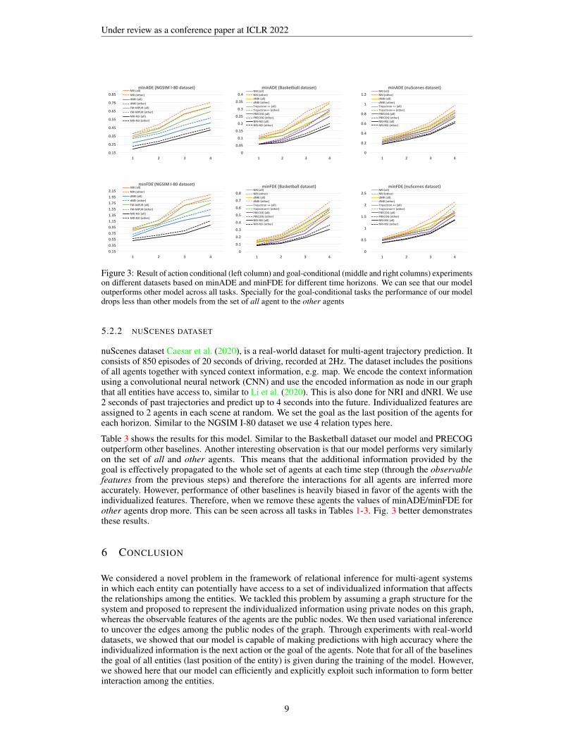
Figure 3: Result of action conditional (left column) and goal-conditional (middle and right columns) experimentson different datasets based on minADE and minFDE for different time horizons. We can see that our modeloutperforms other model across all tasks. Specially for the goal-conditional tasks the performance of our modeldrops less than other models from the set of all agent to the other agents

5.2.2 NUSCENES DATASET

nuScenes dataset Caesar et al. (2020), is a real-world dataset for multi-agent trajectory prediction. Itconsists of 850 episodes of 20 seconds of driving, recorded at 2Hz. The dataset includes the positionsof all agents together with synced context information, e.g. map. We encode the context informationusing a convolutional neural network (CNN) and use the encoded information as node in our graphthat all entities have access to, similar to Li et al. (2020). This is also done for NRI and dNRI. We use2 seconds of past trajectories and predict up to 4 seconds into the future. Individualized features areassigned to 2 agents in each scene at random. We set the goal as the last position of the agents foreach horizon. Similar to the NGSIM I-80 dataset we use 4 relation types here.

Table 3 shows the results for this model. Similar to the Basketball dataset our model and PRECOGoutperform other baselines. Another interesting observation is that our model performs very similarlyon the set of all and other agents. This means that the additional information provided by thegoal is effectively propagated to the whole set of agents at each time step (through the observablefeatures from the previous steps) and therefore the interactions for all agents are inferred moreaccurately. However, performance of other baselines is heavily biased in favor of the agents with theindividualized features. Therefore, when we remove these agents the values of minADE/minFDE forother agents drop more. This can be seen across all tasks in Tables 1-3. Fig. 3 better demonstratesthese results.

6 CONCLUSION

We considered a novel problem in the framework of relational inference for multi-agent systemsin which each entity can potentially have access to a set of individualized information that affectsthe relationships among the entities. We tackled this problem by assuming a graph structure for thesystem and proposed to represent the individualized information using private nodes on this graph,whereas the observable features of the agents are the public nodes. We then used variational inferenceto uncover the edges among the public nodes of the graph. Through experiments with real-worlddatasets, we showed that our model is capable of making predictions with high accuracy where theindividualized information is the next action or the goal of the agents. Note that for all of the baselinesthe goal of all entities (last position of the entity) is given during the training of the model. However,we showed here that our model can efficiently and explicitly exploit such information to form betterinteraction among the entities.

9


REFERENCES

Shaojie Bai, J Zico Kolter, and Vladlen Koltun. An empirical evaluation of generic convolutional andrecurrent networks for sequence modeling. arXiv preprint arXiv:1803.01271, 2018. 2

Holger Caesar, Varun Bankiti, Alex H Lang, Sourabh Vora, Venice Erin Liong, Qiang Xu, AnushKrishnan, Yu Pan, Giancarlo Baldan, and Oscar Beijbom. nuscenes: A multimodal dataset forautonomous driving. In Proceedings of the IEEE/CVF conference on computer vision and patternrecognition, pp. 11621–11631, 2020. 9

Luca Franceschi, Mathias Niepert, Massimiliano Pontil, and Xiao He. Learning discrete structures forgraph neural networks. In International conference on machine learning, pp. 1972–1982. PMLR,2019. 2

Jiyang Gao, Chen Sun, Hang Zhao, Yi Shen, Dragomir Anguelov, Congcong Li, and Cordelia Schmid.Vectornet: Encoding hd maps and agent dynamics from vectorized representation. In Proceedingsof the IEEE/CVF Conference on Computer Vision and Pattern Recognition, pp. 11525–11533,2020. 2

Victor Garcia and Joan Bruna. Few-shot learning with graph neural networks. arXiv preprintarXiv:1711.04043, 2017. 2

Alberto Garcia Duran and Mathias Niepert. Learning graph representations with embedding prop-agation. In I. Guyon, U. V. Luxburg, S. Bengio, H. Wallach, R. Fergus, S. Vishwanathan, andR. Garnett (eds.), Advances in Neural Information Processing Systems, volume 30. Curran As-sociates, Inc., 2017. URL https://proceedings.neurips.cc/paper/2017/file/e0688d13958a19e087e123148555e4b4-Paper.pdf. 2

Colin Graber and Alexander G Schwing. Dynamic neural relational inference. In Proceedings of theIEEE/CVF Conference on Computer Vision and Pattern Recognition, pp. 8513–8522, 2020. 2, 3, 6,8

John Halkias and James Colyar. Ngsim interstate 80 freeway dataset. US Federal Highway Adminis-tration, FHWA-HRT-06-137, Washington, DC, USA, 2006. 7

Will Hamilton, Zhitao Ying, and Jure Leskovec. Inductive representation learning on large graphs. InI. Guyon, U. V. Luxburg, S. Bengio, H. Wallach, R. Fergus, S. Vishwanathan, and R. Gar-nett (eds.), Advances in Neural Information Processing Systems, volume 30. Curran Asso-ciates, Inc., 2017. URL https://proceedings.neurips.cc/paper/2017/file/5dd9db5e033da9c6fb5ba83c7a7ebea9-Paper.pdf. 2

Mikael Henaff, Alfredo Canziani, and Yann LeCun. Model-predictive policy learning with uncertaintyregularization for driving in dense traffic. arXiv preprint arXiv:1901.02705, 2019. 7, 13

Yedid Hoshen. Vain: Attentional multi-agent predictive modeling. arXiv preprint arXiv:1706.06122,2017. 2

Eric Jang, Shixiang Gu, and Ben Poole. Categorical reparameterization with gumbel-softmax. InInternational Conference on Learning Representations (ICLR), 2017. 3

Diederik P Kingma and Jimmy Ba. Adam: A method for stochastic optimization. In ICLR, 2015. 7

Diederik P Kingma and Max Welling. Auto-encoding variational bayes. arXiv preprintarXiv:1312.6114, 2013. 1

Thomas Kipf, Ethan Fetaya, Kuan-Chieh Wang, Max Welling, and Richard Zemel. Neural relationalinference for interacting systems. In International Conference on Machine Learning, pp. 2688–2697. PMLR, 2018. 1, 2, 15

Thomas N Kipf and Max Welling. Semi-supervised classification with graph convolutional networks.2017. 2

Jiachen Li, Fan Yang, Masayoshi Tomizuka, and Chiho Choi. Evolvegraph: Multi-agent trajectoryprediction with dynamic relational reasoning. Proceedings of the Neural Information ProcessingSystems (NeurIPS), 2020. 2, 9

10

https://proceedings.neurips.cc/paper/2017/file/e0688d13958a19e087e123148555e4b4-Paper.pdf

https://proceedings.neurips.cc/paper/2017/file/e0688d13958a19e087e123148555e4b4-Paper.pdf

https://proceedings.neurips.cc/paper/2017/file/5dd9db5e033da9c6fb5ba83c7a7ebea9-Paper.pdf

https://proceedings.neurips.cc/paper/2017/file/5dd9db5e033da9c6fb5ba83c7a7ebea9-Paper.pdf


Yaguang Li, Rose Yu, Cyrus Shahabi, and Yan Liu. Diffusion convolutional recurrent neural network:Data-driven traffic forecasting. In International Conference on Learning Representations, 2018. 2

Yaguang Li, Chuizheng Meng, Cyrus Shahabi, and Yan Liu. Structure-informed graph auto-encoderfor relational inference and simulation. In ICML Workshop on Learning and Reasoning withGraph-Structured Data, volume 8, 2019. 2

Ming Liang, Bin Yang, Rui Hu, Yun Chen, Renjie Liao, Song Feng, and Raquel Urtasun. Learninglane graph representations for motion forecasting. In European Conference on Computer Vision,pp. 541–556. Springer, 2020. 2

Chris J Maddison, Andriy Mnih, and Yee Whye Teh. The concrete distribution: A continuousrelaxation of discrete random variables. 2017. 3

Federico Monti, Davide Boscaini, Jonathan Masci, Emanuele Rodola, Jan Svoboda, and Michael MBronstein. Geometric deep learning on graphs and manifolds using mixture model cnns. InProceedings of the IEEE conference on computer vision and pattern recognition, pp. 5115–5124,2017. 2

Medhini Narasimhan, Svetlana Lazebnik, and Alexander G Schwing. Out of the box: Reasoningwith graph convolution nets for factual visual question answering. 2018. 2

Syama Sundar Rangapuram, Matthias W Seeger, Jan Gasthaus, Lorenzo Stella, Yuyang Wang, andTim Januschowski. Deep state space models for time series forecasting. Advances in neuralinformation processing systems, 31:7785–7794, 2018. 2

Danilo Jimenez Rezende, Shakir Mohamed, and Daan Wierstra. Stochastic backpropagation andapproximate inference in deep generative models. In Proceedings of The 31st InternationalConference on Machine Learning, pp. 1278–1286, 2014. 1

Nicholas Rhinehart, Rowan McAllister, and Sergey Levine. Deep imitative models for flexibleinference, planning, and control. arXiv preprint arXiv:1810.06544, 2018. 3

Nicholas Rhinehart, Rowan McAllister, Kris Kitani, and Sergey Levine. Precog: Prediction condi-tioned on goals in visual multi-agent settings. In Proceedings of the IEEE International Conferenceon Computer Vision, pp. 2821–2830, 2019. 2, 8

Sam T Roweis and Lawrence K Saul. Nonlinear dimensionality reduction by locally linear embedding.science, 290(5500):2323–2326, 2000. 2

David Salinas, Valentin Flunkert, Jan Gasthaus, and Tim Januschowski. Deepar: Probabilisticforecasting with autoregressive recurrent networks. International Journal of Forecasting, 36(3):1181–1191, 2020. 2

Tim Salzmann, Boris Ivanovic, Punarjay Chakravarty, and Marco Pavone. Trajectron++: Dynamically-feasible trajectory forecasting with heterogeneous data. In Proceeding of Europe Conference onComputer Vision (ECCV), 2020. 2, 8

Rajat Sen, Hsiang-Fu Yu, and Inderjit S Dhillon. Think globally, act locally: A deep neural networkapproach to high-dimensional time series forecasting. In H. Wallach, H. Larochelle, A. Beygelzimer,F. d'Alche-Buc, E. Fox, and R. Garnett (eds.), Advances in Neural Information Processing Systems,volume 32. Curran Associates, Inc., 2019. URL https://proceedings.neurips.cc/paper/2019/file/3a0844cee4fcf57de0c71e9ad3035478-Paper.pdf. 2

Joshua B Tenenbaum, Vin De Silva, and John C Langford. A global geometric framework fornonlinear dimensionality reduction. science, 290(5500):2319–2323, 2000. 2

Sjoerd Van Steenkiste, Michael Chang, Klaus Greff, and Jurgen Schmidhuber. Relational neuralexpectation maximization: Unsupervised discovery of objects and their interactions. In ICLR,2017. 2

Petar Velickovic, Guillem Cucurull, Arantxa Casanova, Adriana Romero, Pietro Lio, and YoshuaBengio. Graph attention networks. In ICLR, 2017. 2

11

https://proceedings.neurips.cc/paper/2019/file/3a0844cee4fcf57de0c71e9ad3035478-Paper.pdf

https://proceedings.neurips.cc/paper/2019/file/3a0844cee4fcf57de0c71e9ad3035478-Paper.pdf


Ezra Webb, Ben Day, Helena Andres-Terre, and Pietro Lio. Factorised neural relational inference formulti-interaction systems. arXiv preprint arXiv:1905.08721, 2019. 2

Z Wu, S Pan, G Long, J Jiang, and C Zhang. Graph wavenet for deep spatial-temporal graph modeling.In The 28th International Joint Conference on Artificial Intelligence (IJCAI). International JointConferences on Artificial Intelligence Organization, 2019. 2

Bing Yu, Haoteng Yin, and Zhanxing Zhu. Spatio-temporal graph convolutional networks: adeep learning framework for traffic forecasting. In Proceedings of the 27th International JointConference on Artificial Intelligence, pp. 3634–3640, 2018. 2

Yisong Yue, Patrick Lucey, Peter Carr, Alina Bialkowski, and Iain Matthews. Learning fine-grainedspatial models for dynamic sports play prediction. In 2014 IEEE international conference on datamining, pp. 670–679. IEEE, 2014. 8

12


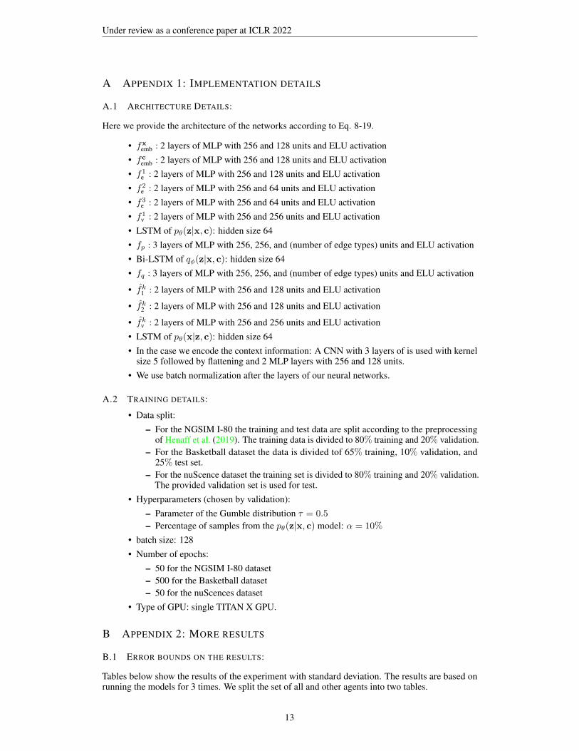
A APPENDIX 1: IMPLEMENTATION DETAILS

A.1 ARCHITECTURE DETAILS:

Here we provide the architecture of the networks according to Eq. 8-19.

• fxemb : 2 layers of MLP with 256 and 128 units and ELU activation• fcemb : 2 layers of MLP with 256 and 128 units and ELU activation• f1e : 2 layers of MLP with 256 and 128 units and ELU activation• f2e : 2 layers of MLP with 256 and 64 units and ELU activation• f3e : 2 layers of MLP with 256 and 64 units and ELU activation• f1v : 2 layers of MLP with 256 and 256 units and ELU activation• LSTM of pθ(z|x, c): hidden size 64• fp : 3 layers of MLP with 256, 256, and (number of edge types) units and ELU activation• Bi-LSTM of qφ(z|x, c): hidden size 64• fq : 3 layers of MLP with 256, 256, and (number of edge types) units and ELU activation

• fk1 : 2 layers of MLP with 256 and 128 units and ELU activation

• fk2 : 2 layers of MLP with 256 and 128 units and ELU activation

• fkv : 2 layers of MLP with 256 and 256 units and ELU activation• LSTM of pθ(x|z, c): hidden size 64• In the case we encode the context information: A CNN with 3 layers of is used with kernel

size 5 followed by flattening and 2 MLP layers with 256 and 128 units.• We use batch normalization after the layers of our neural networks.

A.2 TRAINING DETAILS:

• Data split:– For the NGSIM I-80 the training and test data are split according to the preprocessing

of Henaff et al. (2019). The training data is divided to 80% training and 20% validation.– For the Basketball dataset the data is divided tof 65% training, 10% validation, and

25% test set.– For the nuScence dataset the training set is divided to 80% training and 20% validation.

The provided validation set is used for test.• Hyperparameters (chosen by validation):

– Parameter of the Gumble distribution τ = 0.5

– Percentage of samples from the pθ(z|x, c) model: α = 10%

• batch size: 128• Number of epochs:

– 50 for the NGSIM I-80 dataset– 500 for the Basketball dataset– 50 for the nuScences dataset

• Type of GPU: single TITAN X GPU.

B APPENDIX 2: MORE RESULTS

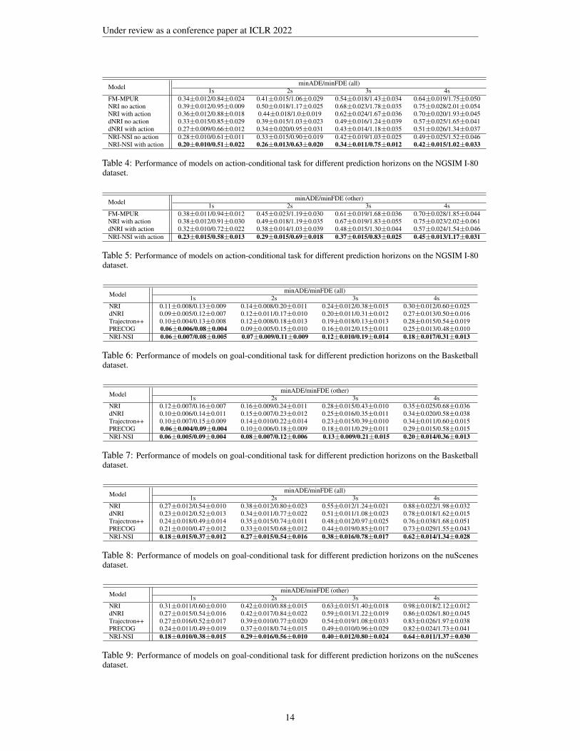
B.1 ERROR BOUNDS ON THE RESULTS:

Tables below show the results of the experiment with standard deviation. The results are based onrunning the models for 3 times. We split the set of all and other agents into two tables.

13


Model minADE/minFDE (all)1s 2s 3s 4s

FM-MPUR 0.34±0.012/0.84±0.024 0.41±0.015/1.06±0.029 0.54±0.018/1.43±0.034 0.64±0.019/1.75±0.050NRI no action 0.39±0.012/0.95±0.009 0.50±0.018/1.17±0.025 0.68±0.023/1.78±0.035 0.75±0.028/2.01±0.054NRI with action 0.36±0.012/0.88±0.018 0.44±0.018/1.0±0.019 0.62±0.024/1.67±0.036 0.70±0.020/1.93±0.045dNRI no action 0.33±0.015/0.85±0.029 0.39±0.015/1.03±0.023 0.49±0.016/1.24±0.039 0.57±0.025/1.65±0.041dNRI with action 0.27±0.009/0.66±0.012 0.34±0.020/0.95±0.031 0.43±0.014/1.18±0.035 0.51±0.026/1.34±0.037NRI-NSI no action 0.28±0.010/0.61±0.011 0.33±0.015/0.90±0.019 0.42±0.019/1.03±0.025 0.49±0.025/1.52±0.046NRI-NSI with action 0.20±0.010/0.51±0.022 0.26±0.013/0.63±0.020 0.34±0.011/0.75±0.012 0.42±0.015/1.02±0.033

Table 4: Performance of models on action-conditional task for different prediction horizons on the NGSIM I-80dataset.

Model minADE/minFDE (other)1s 2s 3s 4s

FM-MPUR 0.38±0.011/0.94±0.012 0.45±0.023/1.19±0.030 0.61±0.019/1.68±0.036 0.70±0.028/1.85±0.044NRI with action 0.38±0.012/0.91±0.030 0.49±0.018/1.19±0.035 0.67±0.019/1.83±0.055 0.75±0.023/2.02±0.061dNRI with action 0.32±0.010/0.72±0.022 0.38±0.014/1.03±0.039 0.48±0.015/1.30±0.044 0.57±0.024/1.54±0.046NRI-NSI with action 0.23±0.015/0.58±0.013 0.29±0.015/0.69±0.018 0.37±0.015/0.83±0.025 0.45±0.013/1.17±0.031

Table 5: Performance of models on action-conditional task for different prediction horizons on the NGSIM I-80dataset.


NRI 0.11±0.008/0.13±0.009 0.14±0.008/0.20±0.011 0.24±0.012/0.38±0.015 0.30±0.012/0.60±0.025dNRI 0.09±0.005/0.12±0.007 0.12±0.011/0.17±0.010 0.20±0.011/0.31±0.012 0.27±0.013/0.50±0.016Trajectron++ 0.10±0.004/0.13±0.008 0.12±0.008/0.18±0.013 0.19±0.018/0.13±0.013 0.28±0.015/0.54±0.019PRECOG 0.06±0.006/0.08±0.004 0.09±0.005/0.15±0.010 0.16±0.012/0.15±0.011 0.25±0.013/0.48±0.010NRI-NSI 0.06±0.007/0.08±0.005 0.07±0.009/0.11±0.009 0.12±0.010/0.19±0.014 0.18±0.017/0.31±0.013











14


B.2 RESULTS ON RELATIONAL INFERENCE

The results in the tables 1-3 show that NRI-NSI performs better than other baselines in terms oftrajectory prediction performance. This might implicitly indicate a better relational inference byNRI-NSI. Nevertheless, here we try to investigate the performance of NRI-NSI compared to NRI anddNRI in terms of relational inference explicitly. We use both toy and real-world datasets for suchinvestigation.

B.2.1 TOY DATASET

Here we use the charged particles dataset. We use 5 and 10 particles in a 2D box with positive andnegative charges {±q} that are sampled uniformly. The force among them follow the Coulomb’slaw. We follow similar procedure by Kipf et al. (2018) to stabilize the generation process, i.e. softclipping the force using the softplus function. Similarly, we generate 50k training examples, and10k validation and test examples. Although the generated data might not exactly follow the physicsrules, we will have explicit relations (force) among the particles and can use this as the ground truthfor our experiments. Our goal is to accurately infer the relation among the particles given that weknow the final position of 1 of the particles for 5-particle experiment and final position of 2 particlesfor 10-particle experiment. For all models we use 2 edge types. For both NRI and dNRI the goalinformation is fed to the last layer of their encoders. Table below shows the accuracy of differentmodels in predicting the relations among the particles:

Toy dataset NRI dNRI NRI-NSI5 particles 82.3 ± 0.5 83.1 ± 0.6 88.5 ± 0.410 particles 70.6 ± 0.5 70.9 ± 0.8 76.8 ± 0.6

Table 10: Performance in terms of relational inference accuracy (in %) for the charged particle dataset.

Note that for this results we only used the encoder of different models.

B.2.2 REAL-WORLD DATASET

The above experiment using the charged particles showcase the superior performance of NRI-NSIcompared to the other two baselines. However, our motivation for proposing NRI-NSI is to incorporateindividualized information. As both action-conditional and goal-conditional trajectory predictionsuggest, such information is meaningful in practice when the agents in the system are autonomous,e.g. we can use the result for planning. In the real-world datasets, however, the relation among theagents are not explicitly defined and there is no ground truth to be used for evaluation of relationinference. Therefore, we designed the following experiment setup:

We chose 100 samples from the nuScenes dataset. For each sample, we used 5 steps (2 seconds)from the past and current time and predicted 8 steps (4 seconds) in the future. In each scene up to 5cars exist, which interact with each other. We used 5 different individuals to decide whether thereshould be any type of interactions among each pair of cars in each scene or not. The individualsagreed on about 94% of the interactions and we used majority vote on their disagreements. If thereshould be any type of interactions among two agents, the ground truth label for the edge betweenthem is 1, and otherwise 0. Then we used NRI, dNRI, and NRI-NSI to uncover the interactionsgiven the goal, similar to the setting in section 5.2.2. Since the type of the interactions uncoveredby the models are not necessarily interpretable by humans in a consistent way, if a model uncoversany type of interaction among two agents, we label that as 1 and otherwise 0. Table below show theaccuracy rate of the different models. We repeat the experiments 5 times by randomly changing thegoal assignments. We also report the recall (sensitivity) rate. It is important for a model to have lownumber of false negatives, i.e. if there is a relationship between two agents the model should be ableto uncover that. NRI-NSI performs better than NRI and dNRI in both metrics. For the real-worlddataset we used the whole structure of all models for relation uncovering over different time steps.

NRI dNRI NRI-NSIAccuracy 84.32 ±0.29 90.45 ± 0.41 94.71 ± 0.50Recall 82.55 ± 0.62 88.64 ± 0.72 93.66 ± 0.38

Table 11: Performance in terms of relational inference accuracy (in %) for the nuScenes dataset

15


As we can see, in both experiments NRI-NSI infers more accurate relations among the agents giventhe individualized information. Therefore, the better performance of NRI-NSI in terms of trajectoryprediction reflected in Tables 1-3 can in fact be a result of better relational inference of the proposedmodel.

16

Documents

N R I NODE-SPECIFIC INFORMATION