Embed Size (px)
Citation preview

FRACTURE MECHANICS

This page intentionally left blank
FRACTURE MECHANICS
by
Nestor PerezDepartment of Mechanical Engineering
University of Puerto Rico
KLUWER ACADEMIC PUBLISHERSNEW YORK, BOSTON, DORDRECHT, LONDON, MOSCOW

eBook ISBN: 1-4020-7861-7Print ISBN: 1-4020-7745-9
©2004 Kluwer Academic PublishersNew York, Boston, Dordrecht, London, Moscow
Print ©2004 Kluwer Academic Publishers
All rights reserved
No part of this eBook may be reproduced or transmitted in any form or by any means, electronic,mechanical, recording, or otherwise, without written consent from the Publisher
Created in the United States of America
Visit Kluwer Online at: http://kluweronline.comand Kluwer's eBookstore at: http://ebooks.kluweronline.com
Boston
Foreword ix
Preface xi
Dedication xiii
1 THEORY OF ELASTICITY 11.11.21.31.41.51.61.71.81.91.101.111.121.13
INTRODUCTION 1DEFINITIONS 2STRAIN AND STRESS EQUATIONS 3TRIAXIAL STRESS STATE 4BIAXIAL STRESS STATE 5SOUND BODIES UNDER TENSION 6PLANE CONDITIONS 10EQUILIBRIUM EQUATIONS 10AIRY’S STRESS FUNCTION 11AIRY’S POWER SERIES 12POLAR COORDINATES 17PROBLEMS 21REFERENCES 23
2 INTRODUCTION TO FRACTURE MECHANICS 252.12.22.32.42.52.62.72.8
INTRODUCTION 25THEORETICAL STRENGTH 26STRESS-CONCENTRATION FACTOR 29GRIFFITH CRACK THEORY 32STRAIN-ENERGY RELEASE RATE 34GRAIN-SIZE REFINEMENT 36PROBLEMS 37REFERENCES 38
CHAPTERS:
Contents
vi CONTENTS
3 LINEAR ELASTIC FRACTURE MECHANICS 393.13.23.3
INTRODUCTION 39MODES OF LOADING 40WESTERGAARD’S STRESS FUNCTION 423.3.13.3.2
FAR-FIELD BOUNDARY CONDITIONS 44NEAR-FIELD BOUNDARY CONDITIONS 45
3.4 SPECIMEN GEOMETRIES 473.4.13.4.23.4.33.4.43.4.5
THROUGH-THE-THICKNESS CENTER CRACK 47ELLIPTICAL CRACKS 51PART-THROUGH THUMBNAIL SURFACE FLAW 53LEAK-BEFORE-BREAK CRITERION 56RADIAL CRACKS AROUND CYLINDERS 58
3.53.63.7
FRACTURE CONTROL 60PLANE STRESS VS. PLANE STRAIN 62PRINCIPLE OF SUPERPOSITION 653.7.1 SINGLE-EDGE CRACKED PLATE (Figure 3.11) 66
3.83.9
PROBLEMS 69REFERENCES 71
4 ELASTIC FIELD EQUATIONS 734.14.24.34.4
INTRODUCTION 73FIELD EQUATIONS: MODE I 73FIELD EQUATIONS: MODE II 77SERIES IN POLAR COORDINATES 804.4.14.4.2
MODE I AND II LOADING CASES 80MODE III LOADING CASE 85
4.54.6
HIGHER ORDER STRESS FIELD 89REFERENCES 93
5 CRACK TIP PLASTICITY 955.15.25.35.45.55.6
INTRODUCTION 95CRACK TIP STRESS STATE 96IRWIN’S APPROXIMATION 98DUGDALE’S APPROXIMATION 101CRACK OPENING DISPLACEMENT 104THE SHAPE OF THE PLASTIC ZONE 1075.6.15.6.2
VON MISES YIELDING CRITERION 108TRESCA YIELDING CRITERION 109
5.75.8
PROBLEMS 116REFERENCES 119
6 THE ENERGY PRINCIPLE 1216.16.26.36.4
INTRODUCTION 121ENERGY RELEASE RATE 121LINEAR COMPLIANCE 123NONLINEAR CRACK GROWTH 125
CONTENTS vii
6.56.66.76.8
TRACTION FORCES 126LOAD AND DISPLACEMENT CONTROL 129CRACK RESISTANCE CURVES 133THE J-INTEGRAL 1356.8.16.8.26.8.3
FRACTURE CRITERION 137CRACK OPENING DISPLACEMENT 138J-INTEGRAL MEASUREMENTS 139
6.96.106.11
TEARING MODULUS 140PROBLEMS 144REFERENCES 145
7 PLASTIC FRACTURE MECHANICS 1477.17.27.37.4
INTRODUCTION 147J-CONTROLLED CRACK GROWTH 147HRR FIELD EQUATIONS 149SEMI-EMPIRICAL APPROACH 1577.4.17.4.2
NEAR-FIELD J-INTEGRAL 159FAR-FIELD J-INTEGRAL 163
7.5 ENGINEERING APPROACH 1637.5.1 THE CONSTANT 167
7.67.7
PROBLEMS 170REFERENCES 171
8 MIXED-MODE FRACTURE MECHANICS 1738.18.28.3
INTRODUCTION 173ELASTIC STATE OF STRESSES 174STRAIN ENERGY RELEASE RATE 1768.3.18.3.28.3.3
MODE I AND II 176FRACTURE ANGLE 179MODE I AND III 181
8.48.58.68.78.8
PRINCIPLE STRESS CRITERION 182STRAIN-ENERGY DENSITY FACTOR 184CRACK BRANCHING 192PROBLEMS 196REFERENCES 197
9 FATIGUE CRACK GROWTH 1999.19.29.39.49.59.69.79.89.9
INTRODUCTION 199CYCLIC STRESS HISTORY 200FATIGUE CRACK INITIATION 203FATIGUE CRACK GROWTH RATE 207FATIGUE LIFE CALCULATIONS 209CRACK GROWTH RATE DIAGRAM 212WELDMENTS 218SURFACE FRACTURE APPEARANCES 220MIXED-MODE LOADING 227
viii CONTENTS
9.10
9.11
9.12
9.13
GROWTH RATE MEASUREMENTS 229
CORROSION FATIGUE 230
PROBLEMS 234
REFERENCES 236
10 FRACTURE TOUGHNESS CORRELATIONS 239
10.1
10.2
10.3
10.4
10.5
10.6
10.7
10.8
10.9
INTRODUCTION 239
CRACK-FREE BODIES UNDER TENSION 239
GRAIN SIZE REFINEMENT 242
INDENTATION-INDUCED CRACKING 244
CHARPY IMPACT TESTING 248
DYNAMIC EFFECTS 251
DYNAMIC STRAIN-ENERGY RELEASE RATE 256
CORRELATIONS 259
SMART HYBRID COMPOSITES 268
10.10
10.11
PROBLEMS 270
REFERENCES 270
A METRIC CONVERSIONS 275
A.1 FRACTURE TOUGHNESS DATA 278
INDEX 279
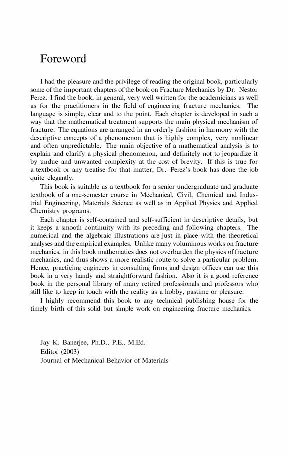
Foreword
I had the pleasure and the privilege of reading the original book, particularlysome of the important chapters of the book on Fracture Mechanics by Dr. NestorPerez. I find the book, in general, very well written for the academicians as wellas for the practitioners in the field of engineering fracture mechanics. Thelanguage is simple, clear and to the point. Each chapter is developed in such away that the mathematical treatment supports the main physical mechanism offracture. The equations are arranged in an orderly fashion in harmony with thedescriptive concepts of a phenomenon that is highly complex, very nonlinearand often unpredictable. The main objective of a mathematical analysis is toexplain and clarify a physical phenomenon, and definitely not to jeopardize itby undue and unwanted complexity at the cost of brevity. If this is true fora textbook or any treatise for that matter, Dr. Perez’s book has done the jobquite elegantly.
This book is suitable as a textbook for a senior undergraduate and graduatetextbook of a one-semester course in Mechanical, Civil, Chemical and Indus-trial Engineering, Materials Science as well as in Applied Physics and AppliedChemistry programs.
Each chapter is self-contained and self-sufficient in descriptive details, butit keeps a smooth continuity with its preceding and following chapters. Thenumerical and the algebraic illustrations are just in place with the theoreticalanalyses and the empirical examples. Unlike many voluminous works on fracturemechanics, in this book mathematics does not overburden the physics of fracturemechanics, and thus shows a more realistic route to solve a particular problem.Hence, practicing engineers in consulting firms and design offices can use thisbook in a very handy and straightforward fashion. Also it is a good referencebook in the personal library of many retired professionals and professors whostill like to keep in touch with the reality as a hobby, pastime or pleasure.
I highly recommend this book to any technical publishing house for thetimely birth of this solid but simple work on engineering fracture mechanics.
Jay K. Banerjee, Ph.D., P.E., M.Ed.Editor (2003)Journal of Mechanical Behavior of Materials

This page intentionally left blank
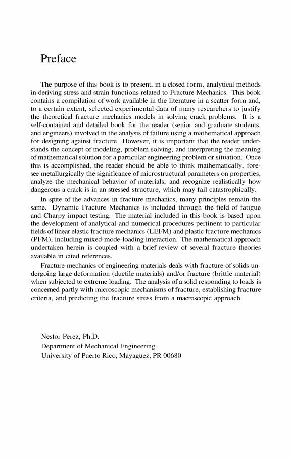
Preface
The purpose of this book is to present, in a closed form, analytical methodsin deriving stress and strain functions related to Fracture Mechanics. This bookcontains a compilation of work available in the literature in a scatter form and,to a certain extent, selected experimental data of many researchers to justifythe theoretical fracture mechanics models in solving crack problems. It is aself-contained and detailed book for the reader (senior and graduate students,and engineers) involved in the analysis of failure using a mathematical approachfor designing against fracture. However, it is important that the reader under-stands the concept of modeling, problem solving, and interpreting the meaningof mathematical solution for a particular engineering problem or situation. Oncethis is accomplished, the reader should be able to think mathematically, fore-see metallurgically the significance of microstructural parameters on properties,analyze the mechanical behavior of materials, and recognize realistically howdangerous a crack is in an stressed structure, which may fail catastrophically.
In spite of the advances in fracture mechanics, many principles remain thesame. Dynamic Fracture Mechanics is included through the field of fatigueand Charpy impact testing. The material included in this book is based uponthe development of analytical and numerical procedures pertinent to particularfields of linear elastic fracture mechanics (LEFM) and plastic fracture mechanics(PFM), including mixed-mode-loading interaction. The mathematical approachundertaken herein is coupled with a brief review of several fracture theoriesavailable in cited references.
Fracture mechanics of engineering materials deals with fracture of solids un-dergoing large deformation (ductile materials) and/or fracture (brittle material)when subjected to extreme loading. The analysis of a solid responding to loads isconcerned partly with microscopic mechanisms of fracture, establishing fracturecriteria, and predicting the fracture stress from a macroscopic approach.
Nestor Perez, Ph.D.
Department of Mechanical EngineeringUniversity of Puerto Rico, Mayaguez, PR 00680

This page intentionally left blank

Dedication
To my wife Neida
To my daughters Jennifer and Roxie
To my son Christopher

This page intentionally left blank
The definition of variables such as force, load, stress, strain, and displacementis vital for the understanding of state properties of solid materials, and forcharacterizing the mechanical behavior of crack-free or cracked solids. Clearly,the latter have a different mechanical behavior than the former and it is char-acterized according to the principles of fracture mechanics, which are dividedinto two areas. Linear Elastic Fracture Mechanics (LEFM) considers the funda-mentals of linear elasticity theory, and Plastic Fracture Mechanics (PFM) is forcharacterizing plastic behavior of ductile solids. In order to characterize crackedsolids, knowledge of the aforementioned variables is necessary. For instance, theterm dynamic force defined by Newton’s second law as depends on theacceleration of a moving mass.
However, if this mass is stationary and susceptible to be deformed a quasi-static force or mechanical force must be defined. Both dynamic and mechanicalforces have the same units, but different physical meaning. Moreover, this me-chanical force is analogous to load (P). Obviously, this is the point of departurein this chapter for defining an important engineering parameter called elasticstress, which in turn it is related to Hooke’s law as Then,is the elastic strain and E is the elastic modulus of elasticity.
Now, the strain is defined as where is the change of dis-placement, say, in the x-direction. The intent here is to indicate how certainparameters or variables are related to one another. Nevertheless, if two vari-ables are known, the third one can be estimated or predicted. This is one of thebenefits of mathematics for solving engineering problems, which have their ownconstraints for dictating the magnitude of a particular variable. In fact, one ormore variables may define a material property, while a property depends on themicrostructure of a solid material.
Chapter 1
THEORY OFELASTICITY
1.1 INTRODUCTION
2 CHAPTER 1. THEORY OF ELASTICITY
1.2 DEFINITIONS
This section is concerned with some definitions the reader needs to assimilatebefore the fracture mechanics theories and mathematical definitions are intro-duced in a progressive manner. It is important to have a clear and precisedefinition of vital concepts in the field of applied mechanics so that the learningprocess for understanding fracture mechanics becomes obviously easy. However,basic concepts such as stress, strain, safety factor, deformation and the like areimportant in characterizing the mechanical behavior of solid materials subjectedto forces or loads in service. Hence,
DEFORMATION: The movement of points in a solid body relative toeach other.
DISPLACEMENT: The movement of a point in a vector quantity in abody subjected to loading.
STRAIN: This is a geometric quantity, which depends on the relative move-ment of two or three points in a body.
STRESS: The stress at a point on a body represents the internal resistanceof a body due to an external force. Thus, load (P) and the cross-sectional area(A) are related to stress as indicated by the equation of equilibrium of forces.Thus,
If A is the original cross-sectional area then is an engineering stress;otherwise, it is a local stress. In addition, the theory of elasticity deals withisotropic materials subjected to elastic stresses, strains, and displacements. Therelationships between stresses and strains are known as constitutive equations,which are classified as Equilibrium Equations, Compatibility Equations andBoundary equations. The reader should consult a book on Theory of Elasticity[1].
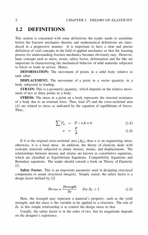
Safety Factor: This is an important parameter used in designing structuralcomponents to assure structural integrity. Simply stated, the safety factor is adesign factor defined by [2]
Here, the strength may represent a material’s property, such as the yieldstrength, and the stress is the variable to be applied to a structure. The role of
in this simple relationship is to control the design stress so thatUsually, the safety factor is in the order of two, but its magnitude depends
on the designer’s experience.
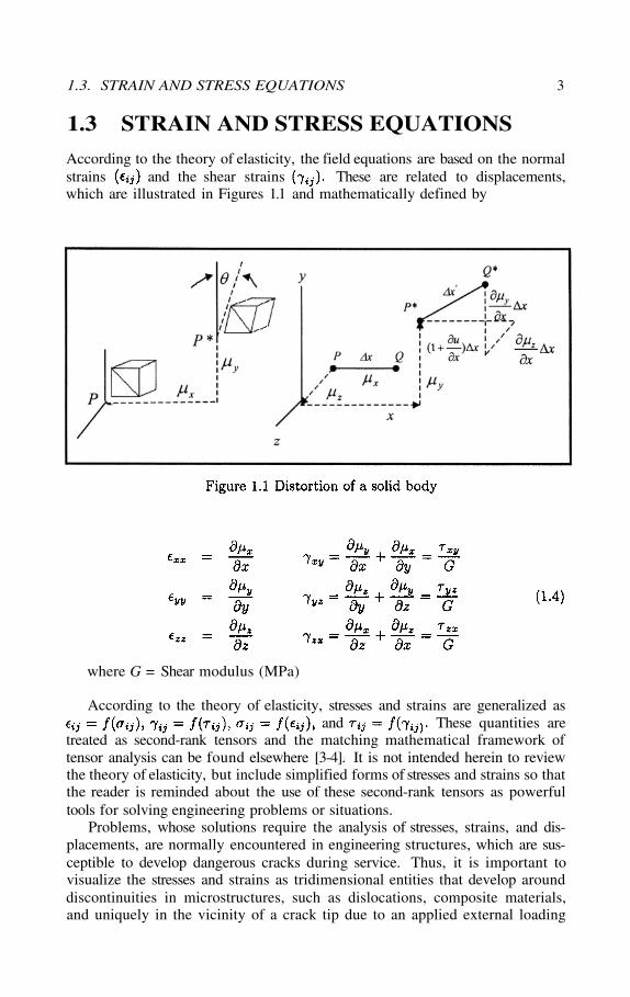
According to the theory of elasticity, the field equations are based on the normalstrains and the shear strains These are related to displacements,which are illustrated in Figures 1.1 and mathematically defined by
where G = Shear modulus (MPa)
According to the theory of elasticity, stresses and strains are generalized asand These quantities are
treated as second-rank tensors and the matching mathematical framework oftensor analysis can be found elsewhere [3-4]. It is not intended herein to reviewthe theory of elasticity, but include simplified forms of stresses and strains so thatthe reader is reminded about the use of these second-rank tensors as powerfultools for solving engineering problems or situations.
Problems, whose solutions require the analysis of stresses, strains, and dis-placements, are normally encountered in engineering structures, which are sus-ceptible to develop dangerous cracks during service. Thus, it is important tovisualize the stresses and strains as tridimensional entities that develop arounddiscontinuities in microstructures, such as dislocations, composite materials,and uniquely in the vicinity of a crack tip due to an applied external loading
1.3. STRAIN AND STRESS EQUATIONS 3
1.3 STRAIN AND STRESS EQUATIONS
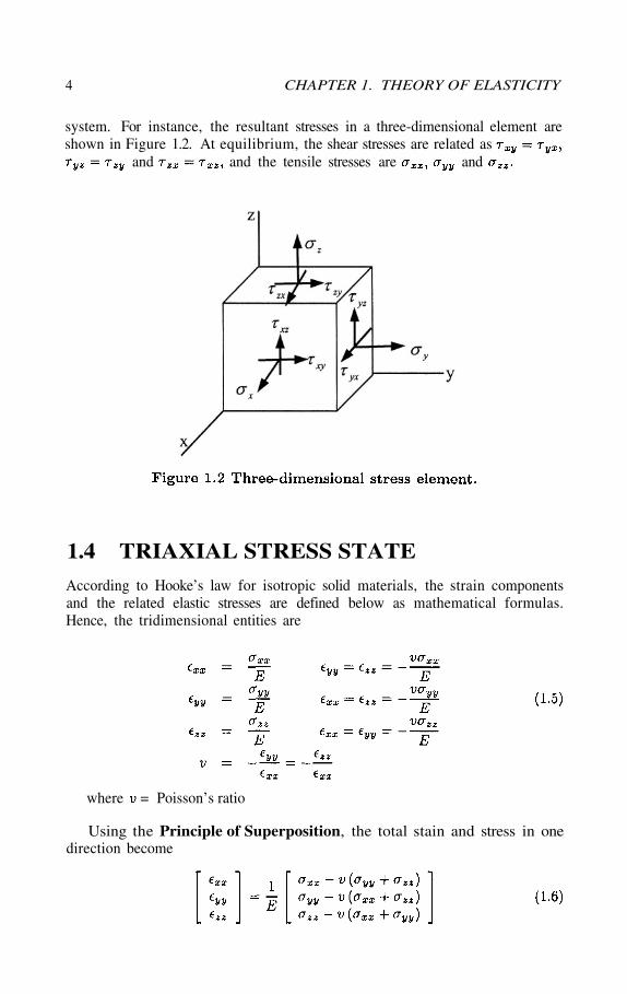
system. For instance, the resultant stresses in a three-dimensional element areshown in Figure 1.2. At equilibrium, the shear stresses are related as
and and the tensile stresses are and
According to Hooke’s law for isotropic solid materials, the strain componentsand the related elastic stresses are defined below as mathematical formulas.Hence, the tridimensional entities are
where = Poisson’s ratio
Using the Principle of Superposition, the total stain and stress in onedirection become
4 CHAPTER 1. THEORY OF ELASTICITY
1.4 TRIAXIAL STRESS STATE
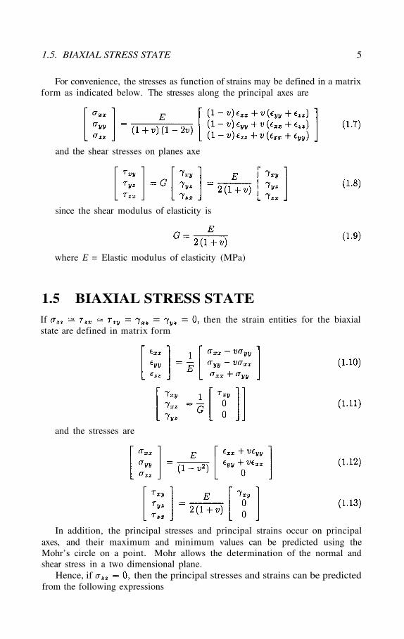
For convenience, the stresses as function of strains may be defined in a matrixform as indicated below. The stresses along the principal axes are
If then the strain entities for the biaxialstate are defined in matrix form
and the stresses are
In addition, the principal stresses and principal strains occur on principalaxes, and their maximum and minimum values can be predicted using theMohr’s circle on a point. Mohr allows the determination of the normal andshear stress in a two dimensional plane.
Hence, if then the principal stresses and strains can be predictedfrom the following expressions
and the shear stresses on planes axe
since the shear modulus of elasticity is
where E = Elastic modulus of elasticity (MPa)
1.5 BIAXIAL STRESS STATE
1.5. BIAXIAL STRESS STATE 5
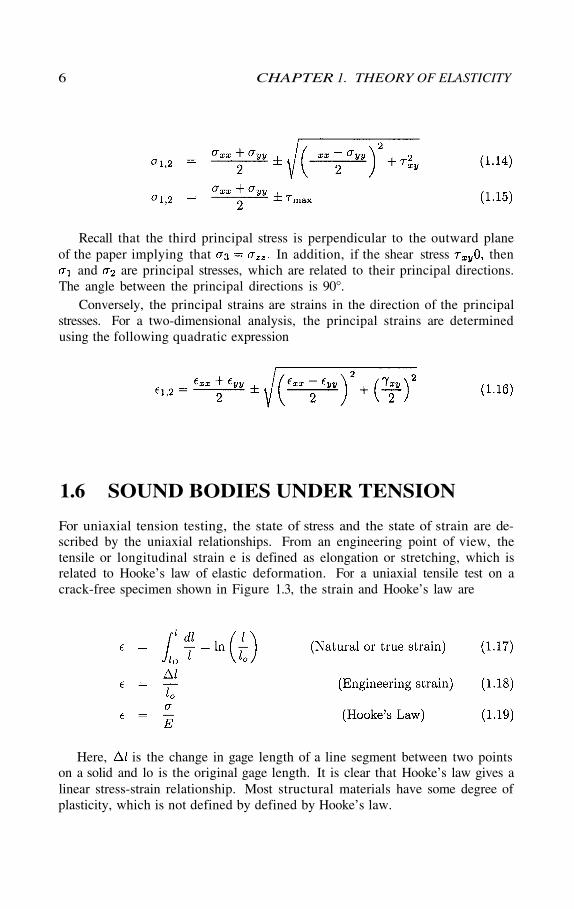
Recall that the third principal stress is perpendicular to the outward planeof the paper implying that In addition, if the shear stress then
and are principal stresses, which are related to their principal directions.The angle between the principal directions is 90°.
Conversely, the principal strains are strains in the direction of the principalstresses. For a two-dimensional analysis, the principal strains are determinedusing the following quadratic expression
For uniaxial tension testing, the state of stress and the state of strain are de-scribed by the uniaxial relationships. From an engineering point of view, thetensile or longitudinal strain e is defined as elongation or stretching, which isrelated to Hooke’s law of elastic deformation. For a uniaxial tensile test on acrack-free specimen shown in Figure 1.3, the strain and Hooke’s law are
6 CHAPTER 1. THEORY OF ELASTICITY
1.6 SOUND BODIES UNDER TENSION
Here, is the change in gage length of a line segment between two pointson a solid and lo is the original gage length. It is clear that Hooke’s law gives alinear stress-strain relationship. Most structural materials have some degree ofplasticity, which is not defined by defined by Hooke’s law.
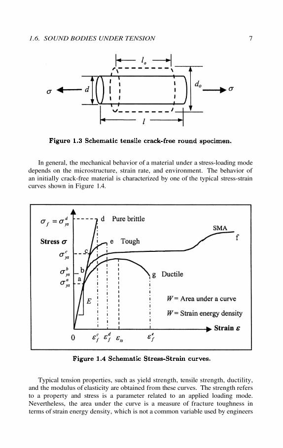
In general, the mechanical behavior of a material under a stress-loading modedepends on the microstructure, strain rate, and environment. The behavior ofan initially crack-free material is characterized by one of the typical stress-straincurves shown in Figure 1.4.
Typical tension properties, such as yield strength, tensile strength, ductility,and the modulus of elasticity are obtained from these curves. The strength refersto a property and stress is a parameter related to an applied loading mode.Nevertheless, the area under the curve is a measure of fracture toughness interms of strain energy density, which is not a common variable used by engineers
1.6. SOUND BODIES UNDER TENSION 7
in structural analysis, but it may be used as a controlling parameter in classifyingstructural materials. Particularly, the SMA curve in Figure 1.4 is for a shapememory alloy (SMA), such as 55Ni-45Ti (Nitinol), which exhibits significanthigh strain to failure (superelastic) and high total strain energy density [5–6].
This strain energy density W is the energy required to deformthe material. According to Figure 1.4, this energy is the area under the curve.For elastic behavior (up to the yield point), fracture toughness is the elasticstrain energy density known as resilience and it is defined as
8 CHAPTER 1. THEORY OF ELASTICITY
This expression represents an elastic behavior up to the yield strain for pointsa, b, c and d in Figure 1.4. Hooke’s law, eq. (1.19), is used to solve the integralgiven by eq. (1.20). Thus, the elastic strain energy density becomes
On the other hand, tough materials have fracture toughness based onand SMA curves. Thus, the strain energy density for curve takes the form
This integral can be solved once a stress function in terms of strain,is available. The most common plastic stress functions applicable from theyield point to the ultimate tensile stress (maximum stress on a stress-straincurves (Figure 1.4). are known as Ramberg-Osgood and Hollomon equations.These functions are defined by
where = Strain hardening exponents= Strength coefficient or proportionality constant (MPa)= Plastic stress (MPa)
=Yield strength (MPa)= Plastic strain
= Constant
For a strain hardenable material, the Hollomon or power-law equation maybe used as an effective stress expression in eq. (10.3) so that the integral can
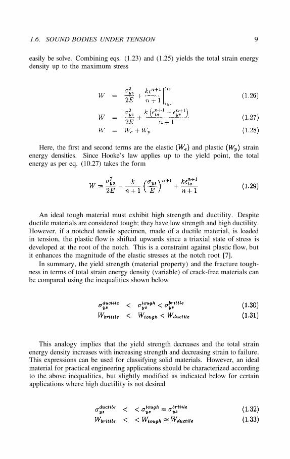
easily be solve. Combining eqs. (1.23) and (1.25) yields the total strain energydensity up to the maximum stress
Here, the first and second terms are the elastic and plastic strainenergy densities. Since Hooke’s law applies up to the yield point, the totalenergy as per eq. (10.27) takes the form
An ideal tough material must exhibit high strength and ductility. Despiteductile materials are considered tough; they have low strength and high ductility.However, if a notched tensile specimen, made of a ductile material, is loadedin tension, the plastic flow is shifted upwards since a triaxial state of stress isdeveloped at the root of the notch. This is a constraint against plastic flow, butit enhances the magnitude of the elastic stresses at the notch root [7].
In summary, the yield strength (material property) and the fracture tough-ness in terms of total strain energy density (variable) of crack-free materials canbe compared using the inequalities shown below
This analogy implies that the yield strength decreases and the total strainenergy density increases with increasing strength and decreasing strain to failure.This expressions can be used for classifying solid materials. However, an idealmaterial for practical engineering applications should be characterized accordingto the above inequalities, but slightly modified as indicated below for certainapplications where high ductility is not desired
1.6. SOUND BODIES UNDER TENSION 9
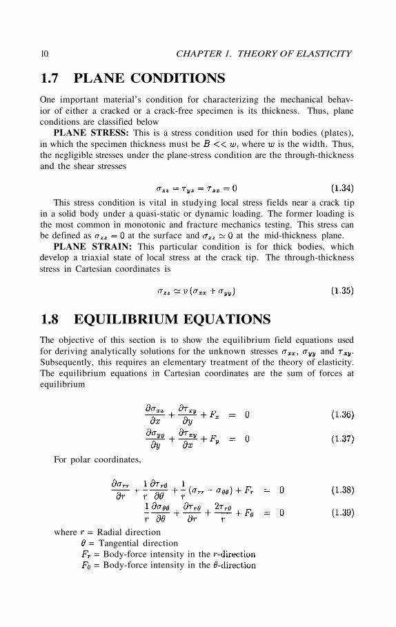
One important material’s condition for characterizing the mechanical behav-ior of either a cracked or a crack-free specimen is its thickness. Thus, planeconditions are classified below
PLANE STRESS: This is a stress condition used for thin bodies (plates),in which the specimen thickness must be where is the width. Thus,the negligible stresses under the plane-stress condition are the through-thicknessand the shear stresses
10 CHAPTER 1. THEORY OF ELASTICITY
1.7 PLANE CONDITIONS
This stress condition is vital in studying local stress fields near a crack tipin a solid body under a quasi-static or dynamic loading. The former loading isthe most common in monotonic and fracture mechanics testing. This stress canbe defined as at the surface and at the mid-thickness plane.
PLANE STRAIN: This particular condition is for thick bodies, whichdevelop a triaxial state of local stress at the crack tip. The through-thicknessstress in Cartesian coordinates is
1.8 EQUILIBRIUM EQUATIONSThe objective of this section is to show the equilibrium field equations usedfor deriving analytically solutions for the unknown stresses andSubsequently, this requires an elementary treatment of the theory of elasticity.The equilibrium equations in Cartesian coordinates are the sum of forces atequilibrium
For polar coordinates,
where = Radial direction= Tangential direction
= Body-force intensity in the= Body-force intensity in the
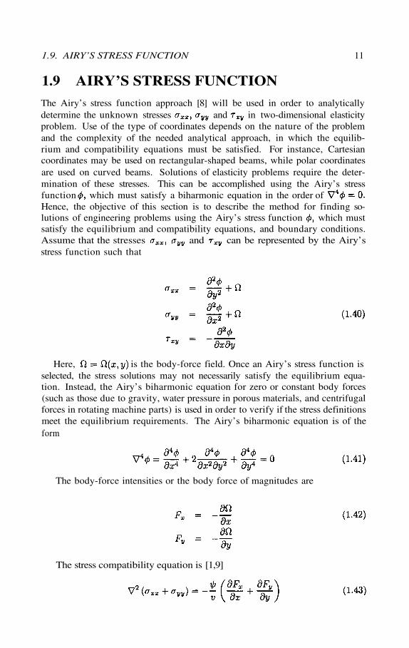
The Airy’s stress function approach [8] will be used in order to analyticallydetermine the unknown stresses and in two-dimensional elasticityproblem. Use of the type of coordinates depends on the nature of the problemand the complexity of the needed analytical approach, in which the equilib-rium and compatibility equations must be satisfied. For instance, Cartesiancoordinates may be used on rectangular-shaped beams, while polar coordinatesare used on curved beams. Solutions of elasticity problems require the deter-mination of these stresses. This can be accomplished using the Airy’s stressfunction which must satisfy a biharmonic equation in the order ofHence, the objective of this section is to describe the method for finding so-lutions of engineering problems using the Airy’s stress function which mustsatisfy the equilibrium and compatibility equations, and boundary conditions.Assume that the stresses and can be represented by the Airy’sstress function such that
1.9. AIRY’S STRESS FUNCTION 11
1.9 AIRY’S STRESS FUNCTION
Here, is the body-force field. Once an Airy’s stress function isselected, the stress solutions may not necessarily satisfy the equilibrium equa-tion. Instead, the Airy’s biharmonic equation for zero or constant body forces(such as those due to gravity, water pressure in porous materials, and centrifugalforces in rotating machine parts) is used in order to verify if the stress definitionsmeet the equilibrium requirements. The Airy’s biharmonic equation is of theform
The body-force intensities or the body force of magnitudes are
The stress compatibility equation is [1,9]
Any Airy’s stress function used in the solution of engineering problemsshould satisfy eq. (1.41). Subsequently, the stresses can be derived using eq.(1.40). However, the type of function one chooses should be based on experi-ence or trial and error so that satisfies eq. (1.41).
It should be mentioned that the Airy’s stress function is also used fordetermining the stress field, and subsequently the strain field around edge dislo-cations in an isotropic and continuous media. A mathematical and theoreticaltreatment on this particular subject is given in a book written by Meyers andChawla [3] in which clear isostress contours indicate the maximum tension, com-pression, and shear stresses.
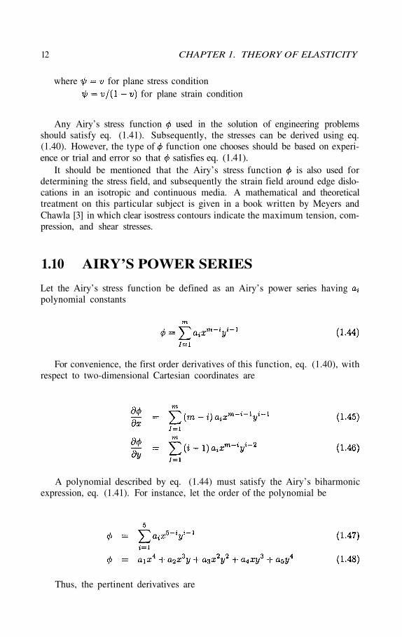
Let the Airy’s stress function be defined as an Airy’s power series havingpolynomial constants
For convenience, the first order derivatives of this function, eq. (1.40), withrespect to two-dimensional Cartesian coordinates are
A polynomial described by eq. (1.44) must satisfy the Airy’s biharmonicexpression, eq. (1.41). For instance, let the order of the polynomial be
Thus, the pertinent derivatives are
12 CHAPTER 1. THEORY OF ELASTICITY
where for plane stress conditionfor plane strain condition
1.10 AIRY’S POWER SERIES
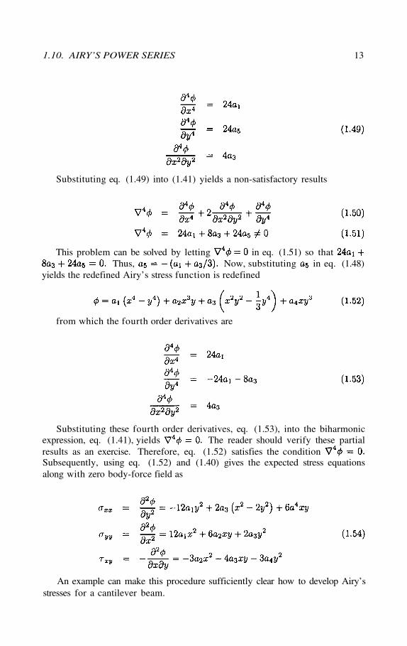
Substituting these fourth order derivatives, eq. (1.53), into the biharmonicexpression, eq. (1.41), yields The reader should verify these partialresults as an exercise. Therefore, eq. (1.52) satisfies the conditionSubsequently, using eq. (1.52) and (1.40) gives the expected stress equationsalong with zero body-force field as
An example can make this procedure sufficiently clear how to develop Airy’sstresses for a cantilever beam.
1.10. AIRY’S POWER SERIES 13
Substituting eq. (1.49) into (1.41) yields a non-satisfactory results
This problem can be solved by letting in eq. (1.51) so thatThus, Now, substituting in eq. (1.48)
yields the redefined Airy’s stress function is redefined
from which the fourth order derivatives are
14 CHAPTER 1. THEORY OF ELASTICITY
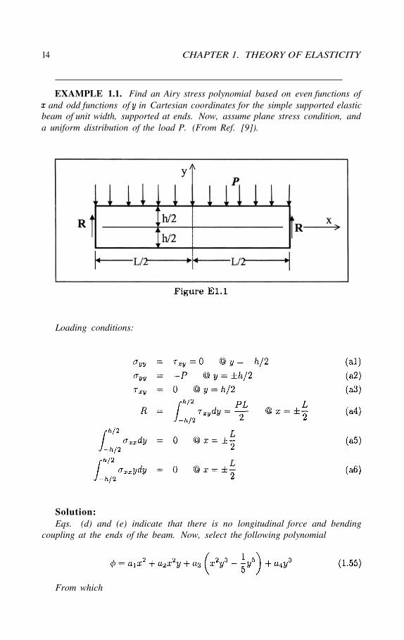
EXAMPLE 1.1. Find an Airy stress polynomial based on even functions ofand odd functions of in Cartesian coordinates for the simple supported elastic
beam of unit width, supported at ends. Now, assume plane stress condition, anda uniform distribution of the load P. (From Ref. [9]).
Loading conditions:
Eqs. (d) and (e) indicate that there is no longitudinal force and bendingcoupling at the ends of the beam. Now, select the following polynomial
From which
Solution:
Solving eqs. (b1) and (b2) simultaneously for yields
1.10. AIRY’S POWER SERIES 15
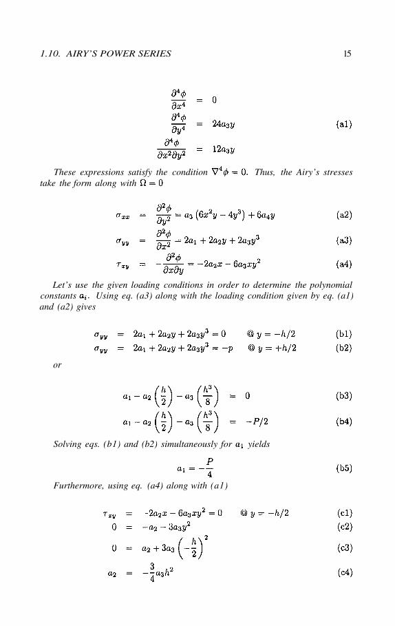
These expressions satisfy the condition Thus, the Airy’s stressestake the form along with
Let’s use the given loading conditions in order to determine the polynomialconstants Using eq. (a3) along with the loading condition given by eq. (a1)and (a2) gives
or
Furthermore, using eq. (a4) along with (a1)
16 CHAPTER 1. THEORY OF ELASTICITY
Substituting eqs. (b5) and (c4) into (b3) gives
Combining eqs. (a6) and (a2) yields
Solving this integral and using eq. (c5) gives
Using the moment of inertia in eq. (d6) yields
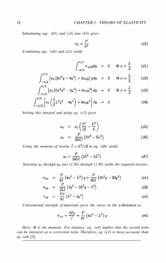
Inserting through into (1.56) through (1.58) yields the required stresses
Conventional strength of materials gives the stress in the as
Here, M is the moment. For instance, eq. (e4) implies that the second termcan be interpret as a correction term. Therefore, eq. (e1) is more accurate thaneq. (e4) [3].
1.11. POLAR COORDINATES 17
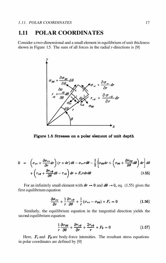
Consider a two-dimensional and a small element in equilibrium of unit thicknessshown in Figure 1.5. The sum of all forces in the radial r-directions is [9]
For an infinitely small element with and eq. (1.55) gives thefirst equilibrium equation
Similarly, the equilibrium equation in the tangential direction yields thesecond equilibrium equation
Here, and are body-force intensities. The resultant stress equationsin polar coordinates are defined by [9]
1.11 POLAR COORDINATES
18 CHAPTER 1. THEORY OF ELASTICITY
One particular Airy’s stress function for a crack-free hollow cylinder is ofthe type [9]
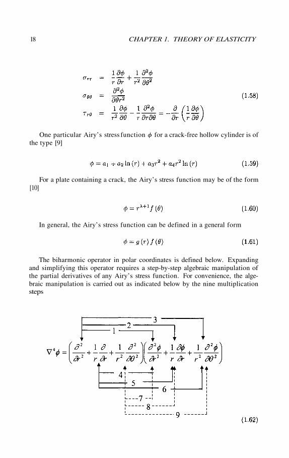
The biharmonic operator in polar coordinates is defined below. Expandingand simplifying this operator requires a step-by-step algebraic manipulation ofthe partial derivatives of any Airy’s stress function. For convenience, the alge-braic manipulation is carried out as indicated below by the nine multiplicationsteps
For a plate containing a crack, the Airy’s stress function may be of the form[10]
In general, the Airy’s stress function can be defined in a general form
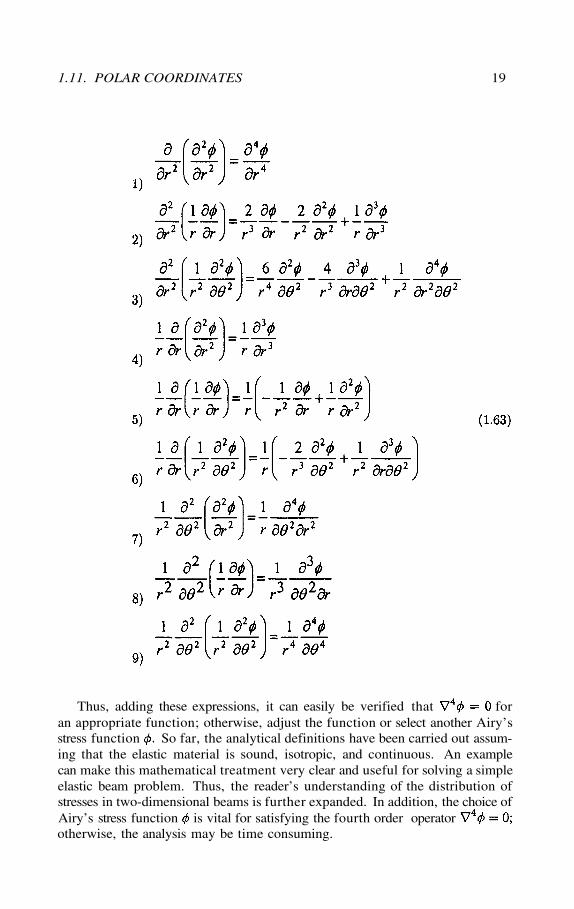
Thus, adding these expressions, it can easily be verified that foran appropriate function; otherwise, adjust the function or select another Airy’sstress function So far, the analytical definitions have been carried out assum-ing that the elastic material is sound, isotropic, and continuous. An examplecan make this mathematical treatment very clear and useful for solving a simpleelastic beam problem. Thus, the reader’s understanding of the distribution ofstresses in two-dimensional beams is further expanded. In addition, the choice ofAiry’s stress function is vital for satisfying the fourth order operatorotherwise, the analysis may be time consuming.
1.11. POLAR COORDINATES 19
20 CHAPTER 1. THEORY OF ELASTICITY
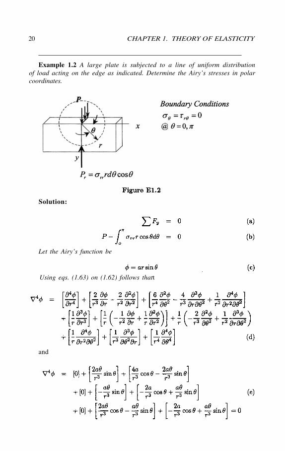
Example 1.2 A large plate is subjected to a line of uniform distributionof load acting on the edge as indicated. Determine the Airy’s stresses in polarcoordinates.
Solution:
Let the Airy’s function be
and
Using eqs. (1.63) on (1.62) follows thatt
1.12. PROBLEMS 21
Therefore, eq. (c) satisfies Furthermore, the elastic stresses can bedefined in terms of trigonometric functions. According to eq. (1.58), the elasticstresses in polar coordinates are
These results imply that the boundary conditions were correct. Combiningeqs. (b) and (f) provides the final expression for the load P and the constant a
Substituting eq. (i3) into (f) yields the radial stress
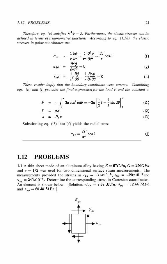
1.1 A thin sheet made of an aluminum alloy havingand was used for two dimensional surface strain measurements. Themeasurements provided the strains as and
Determine the corresponding stress in Cartesian coordinates.An element is shown below. [Solution:and
1.12 PROBLEMS
22 CHAPTER 1. THEORY OF ELASTICITY
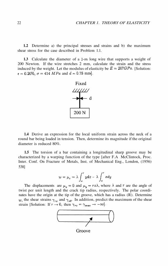
1.3 Calculate the diameter of a long wire that supports a weight of200 Newton. If the wire stretches 2 mm, calculate the strain and the stressinduced by the weight. Let the modulus of elasticity be [Solution:
and
1.4 Derive an expression for the local uniform strain across the neck of around bar being loaded in tension. Then, determine its magnitude if the originaldiameter is reduced 80%.
1.2 Determine a) the principal stresses and strains and b) the maximumshear stress for the case described in Problem 1.1.
1.5 The torsion of a bar containing a longitudinal sharp groove may becharacterized by a warping function of the type [after F.A McClintock, Proc.Inter. Conf. On Fracture of Metals, Inst. of Mechanical Eng., London, (1956)538]
The displacements are and where and are the angle oftwist per unit length and the crack tip radius, respectively. The polar coordi-nates have the origin at the tip of the groove, which has a radius (R). Determine
the shear strains and In addition, predict the maximum of the shearstrain [Solution: If then
1.13. REFERENCES 23
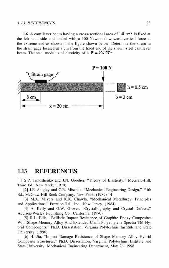
1.6 A cantilever beam having a cross-sectional area of is fixed atthe left-hand side and loaded with a 100 Newton downward vertical force atthe extreme end as shown in the figure shown below. Determine the strain inthe strain gage located at 8 cm from the fixed end of the shown steel cantileverbeam. The steel modulus of elasticity of is
1.13 REFERENCES[1] S.P. Timoshenko and J.N. Goodier, “Theory of Elasticity,” McGraw-Hill,Third Ed., New York, (1970)
[2] J.E. Shigley and C.R. Mischke, “Mechanical Engineering Design,” FifthEd., McGraw-Hill Book Company, New York, (1989) 14
[3] M.A. Meyers and K.K. Chawla, “Mechanical Metallurgy: Principlesand Applications,” Prentice-Hall, Inc., New Jersey, (1984)
[4] A. Kelly and G.W. Groves, “Crystallography and Crystal Defects,”Addison-Wesley Publishing Co., California, (1970)
[5] R.L. Ellis, “Ballistic Impact Resistance of Graphite Epoxy CompositesWith Shape Memory Alloy And Extended Chain Polyethylene Spectra TM Hy-brid Components,” Ph.D. Dissertation, Virginia Polytechnic Institute and StateUniversity, (1996)
[6] H. Jia, “Impact Damage Resistance of Shape Memory Alloy HybridComposite Structures,” Ph.D. Dissertation, Virginia Polytechnic Institute andState University, Mechanical Engineering Department, May 26, 1998

[7] W.S. Peeling, “Design Options for Selection of Fracture Control Pro-cedures in the Modernization of Codes, Rules, and Standards,” Proceedings:Joint United States–Japan Symposium on Applications of Pressure ComponentCodes, Tokyo, Japan. (March 1973)
[8] G.B. Airy, British Assoc. Adv. Sci. Report, (1862)[9] J.W. Dally and W.F. Riley, “Experimental Stress Analysis,” Third
edition, McGraw-Hill, New York, (1991)[10] K. Hellan, “Introduction to Fracture Mechanics,” McGraw-Hill Book
company, New York, (1984)
24 CHAPTER 1. THEORY OF ELASTICITY
Chapter 2
INTRODUCTION TOFRACTURE MECHANICS
2.1 INTRODUCTION
The theory of elasticity used in Chapter 1 served the purpose of illustrating theclose form of analytical procedures in order to develop constitutive equations forpredicting failure of crack-free solids [1]. However, when solids contain flaws orcracks, the field equations are not completely defined by the theory of elasticitysince it does not consider the stress singularity phenomenon near a crack tip.It only provides the means to predict general yielding as a failure criterion.Despite the usefulness of predicting yielding, it is necessary to use the principlesof fracture mechanics to predict fracture of solid components containing cracks.
fracture mechanics is the study of mechanical behavior of cracked materialssubjected to an applied load. In fact, Irwin [2] developed the field of frac-ture mechanics using the early work of Inglis [3], Griffith [4], and Westergaard[5]. Essentially, fracture mechanics deals with the irreversible process of rup-ture due to nucleation and growth of cracks. The formation of cracks may bea complex fracture process, which strongly depends on the microstructure ofa particular crystalline or amorphous solid, applied loading, and environment.The microstructure plays a very important role in a fracture process due to dis-location motion, precipitates, inclusions, grain size, and type of phases makingup the microstructure. All these microstructural features are imperfections andcan act as fracture nuclei under unfavorable conditions. For instance, BrittleFracture is a low-energy process (low energy dissipation), which may lead tocatastrophic failure without warning since the crack velocity is normally high.Therefore, little or no plastic deformation may be involved before separationof the solid. On the other hand, Ductile Fracture is a high-energy processin which a large amount of energy dissipation is associated with a large plasticdeformation before crack instability occurs. Consequently, slow crack growthoccurs due to strain hardening at the crack tip region.
26 CHAPTER 2. INTRODUCTION TO FRACTURE MECHANICS
2.2 THEORETICAL STRENGTH
Consider the predicament of how strong a perfect (ideal) crystal lattice should beunder an applied state of stress, and the comparison of the actual and theoreticalstrength of metals. This is a very laborious work to perform, but theoretical ap-proximations can be made in order to determine or calculate the stress requiredfor fracture of atomic bonding in crystalline or amorphous crystals.
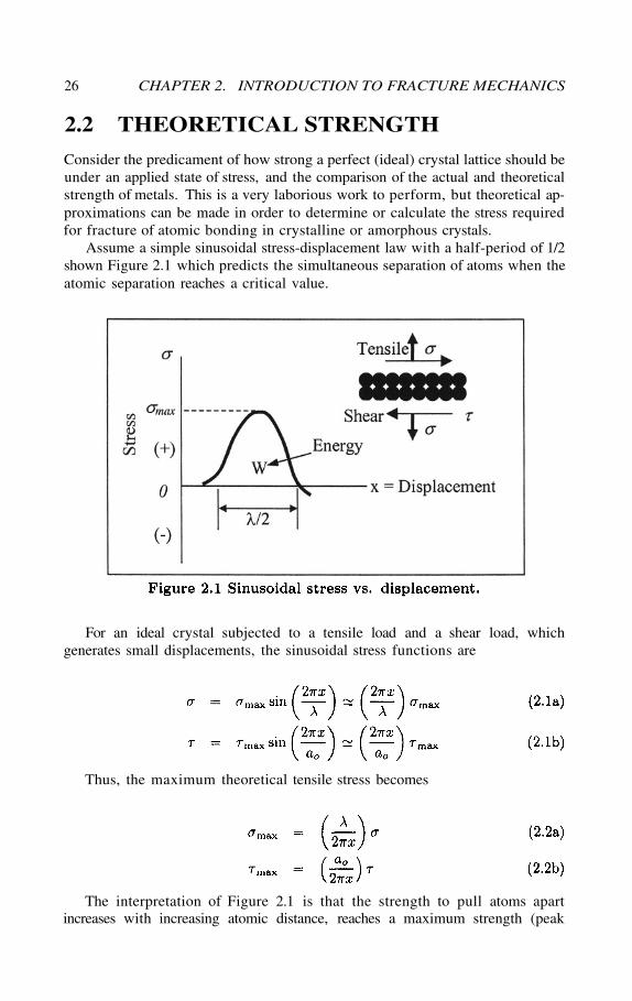
Assume a simple sinusoidal stress-displacement law with a half-period of 1/2shown Figure 2.1 which predicts the simultaneous separation of atoms when theatomic separation reaches a critical value.
For an ideal crystal subjected to a tensile load and a shear load, whichgenerates small displacements, the sinusoidal stress functions are
Thus, the maximum theoretical tensile stress becomes
The interpretation of Figure 2.1 is that the strength to pull atoms apartincreases with increasing atomic distance, reaches a maximum strength (peak
2.2. THEORETICAL STRENGTH 27
strength) equals to the theoretical (cohesive) tensile strength andthen it decreases as atoms are further apart in the direction perpendicular to theapplied stress. Consequently, atomic planes separate and the material cleavesperpendicularly to the tensile stress.
Assuming an elastic deformation process, Hooke’s law gives the tensile andshear modulus of elasticity defined by
where Equilibrium atomic distance (Figure 2.2)
Combining eqs. (2.2) and (2.3) yields the theoretical fracture strength ofsolid materials
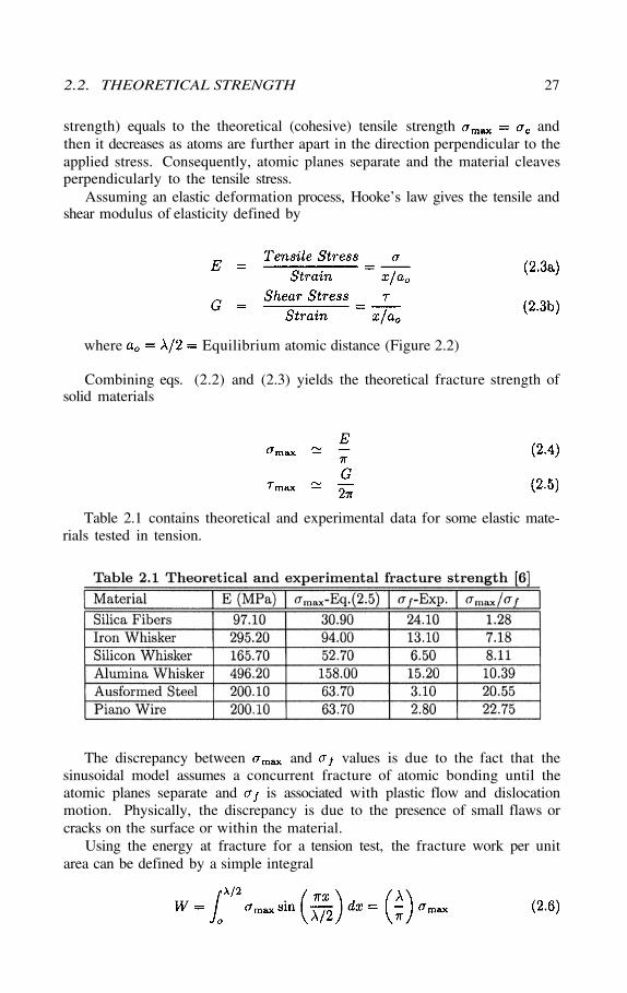
Table 2.1 contains theoretical and experimental data for some elastic mate-rials tested in tension.
The discrepancy between and values is due to the fact that thesinusoidal model assumes a concurrent fracture of atomic bonding until theatomic planes separate and is associated with plastic flow and dislocationmotion. Physically, the discrepancy is due to the presence of small flaws orcracks on the surface or within the material.
Using the energy at fracture for a tension test, the fracture work per unitarea can be defined by a simple integral
28 CHAPTER 2. INTRODUCTION TO FRACTURE MECHANICS
Letting be the total surface energy required to form two new fracturesurfaces and combining eqs. (2.4) and (2.6) yields the theoretical tensile strengthin terms of surface energy and equilibrium spacing
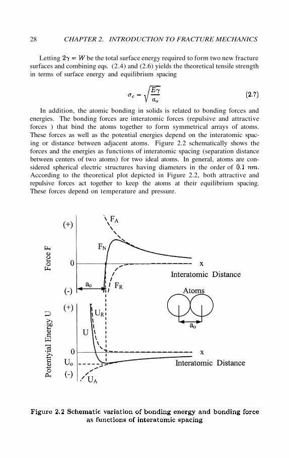
In addition, the atomic bonding in solids is related to bonding forces andenergies. The bonding forces are interatomic forces (repulsive and attractiveforces ) that bind the atoms together to form symmetrical arrays of atoms.These forces as well as the potential energies depend on the interatomic spac-ing or distance between adjacent atoms. Figure 2.2 schematically shows theforces and the energies as functions of interatomic spacing (separation distancebetween centers of two atoms) for two ideal atoms. In general, atoms are con-sidered spherical electric structures having diameters in the order ofAccording to the theoretical plot depicted in Figure 2.2, both attractive andrepulsive forces act together to keep the atoms at their equilibrium spacing.These forces depend on temperature and pressure.
2.3. STRESS-CONCENTRATION FACTOR 29
The potential or bonding energy and forces are defined by
where = Attractive constant = Repulsive constant= Exponents
= Attractive and repulsive energies= Attractive and repulsive forces
The curves in Figure 2.2 are known as Condon-Morse curves and are usedto explain the physical events of atomic displacement at a nanoscale. At equi-librium, the minimum potential energy and the net force are dependent of theinteratomic spacing; that is, and However,if the interatomic spacing is slightly decreased or perturbed by theaction of an applied load, a repulsive force builds up and the two atoms havethe tendency to return to their equilibrium position at On the otherhand, if an attractive force builds up so that
Conclusively, an array of atoms form a definite atomic pattern with respectto their neighboring atoms and as a result, all atoms form a specific spacelattice consisting of unit cells, such as body-centered cubic (BCC), hexagonal.,monoclinic and the like.
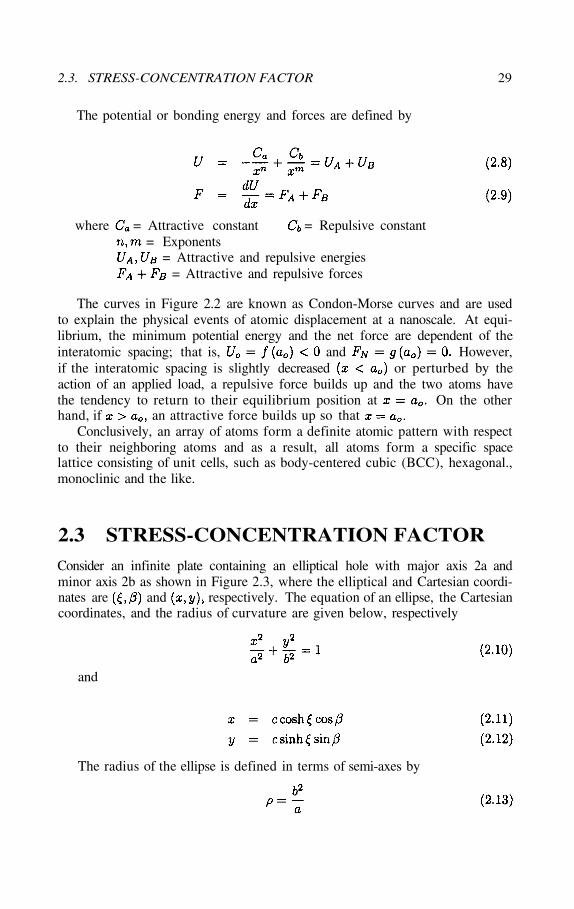
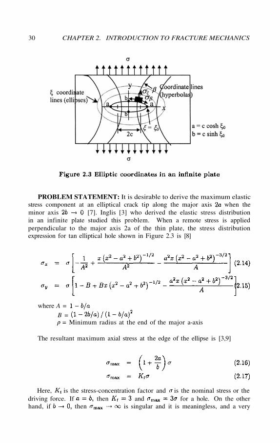
2.3 STRESS-CONCENTRATION FACTORConsider an infinite plate containing an elliptical hole with major axis 2a andminor axis 2b as shown in Figure 2.3, where the elliptical and Cartesian coordi-nates are and respectively. The equation of an ellipse, the Cartesiancoordinates, and the radius of curvature are given below, respectively
and
The radius of the ellipse is defined in terms of semi-axes by
30 CHAPTER 2. INTRODUCTION TO FRACTURE MECHANICS
PROBLEM STATEMENT: It is desirable to derive the maximum elasticstress component at an elliptical crack tip along the major axis when theminor axis [7]. Inglis [3] who derived the elastic stress distributionin an infinite plate studied this problem. When a remote stress is appliedperpendicular to the major axis 2a of the thin plate, the stress distributionexpression for tan elliptical hole shown in Figure 2.3 is [8]
where A =
B == Minimum radius at the end of the major a-axis
The resultant maximum axial stress at the edge of the ellipse is [3,9]
Here, is the stress-concentration factor and is the nominal stress or thedriving force. If then and for a hole. On the otherhand, if then is singular and it is meaningless, and a very
2.3. STRESS-CONCENTRATION FACTOR 31
sharp crack is formed since In addition, is used to analyze the a stressat a point in the vicinity of a notch having a radius However, if a crackis formed having the stress field at the crack tip is defined in terms ofthe stress-intensity factor instead of the stress-concentration factorIn fact, microstructural discontinuities and geometrical discontinuities, such asnotches, holes, grooves, and the like, are sources for crack initiation when thestress-concentration factor is sufficiently high. The degree of concentration ofthe stresses or strains is determined as the stress-concentration factor.
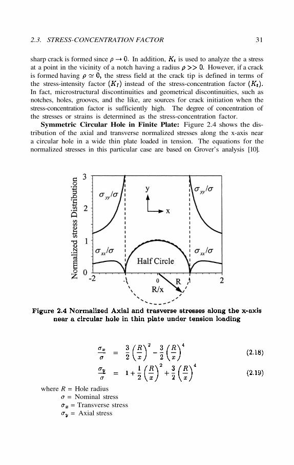
Symmetric Circular Hole in Finite Plate: Figure 2.4 shows the dis-tribution of the axial and transverse normalized stresses along the x-axis neara circular hole in a wide thin plate loaded in tension. The equations for thenormalized stresses in this particular case are based on Grover’s analysis [10].
where R = Hole radius= Nominal stress= Transverse stress= Axial stress
32 CHAPTER 2. INTRODUCTION TO FRACTURE MECHANICS
2.4 GRIFFITH CRACK THEORY
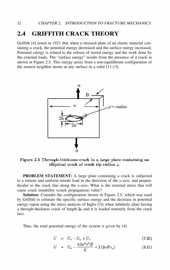
Griffith [4] noted in 1921 that when a stressed plate of an elastic material con-taining a crack, the potential energy decreased and the surface energy increased.Potential energy is related to the release of stored energy and the work done bythe external loads. The “surface energy” results from the presence of a crack asshown in Figure 2.5. This energy arises from a non-equilibrium configuration ofthe nearest neighbor atoms at any surface in a solid [11-13].
PROBLEM STATEMENT: A large plate containing a crack is subjectedto a remote and uniform tensile load in the direction of the y-axis, and perpen-dicular to the crack line along the x-axis. What is the external stress that willcause crack instability (crack propagation) value?
Solution: Consider the configuration shown in Figure 2.5, which was usedby Griffith to estimate the specific surface energy and the decrease in potentialenergy (upon using the stress analysis of Inglis [3]) when infinitely plate havinga through-thickness crack of length and it is loaded remotely from the crackface.
Thus, the total potential energy of the system is given by [4]
2.4. GRIFFITH CRACK THEORY 33
where U = Potential energy of the cracked body= Potential energy of uncracked body= Elastic energy due to the presence of the crack= Elastic-surface energy due to the formation of crack surfaces
= One-half crack length= = Total surface crack area
= Specific surface energyE = Modulus of elasticity
= Applied stress and = Poisson’s ratio= 1 for plane stress and for plane strain
The equilibrium condition of eq. (2.21) is defined by the first order partialderive. The equilibrium condition of eq. (2.21) is defined by the first orderderivative with respect to crack length. This derivative is of significance becausethe critical crack size may be predicted very easily. If the crack sizeand total surface energy are, respectively
Rearranging eq. (2.23) gives a significant expression in linear elastic fracturemechanics (LEFM)
The parameter is called the stress intensity factor which is the crackdriving force and its critical value is a material property known as fracturetoughness, which in turn, is the resistance force to crack extension [14]. Theinterpretation of eq. (2.24) suggests that crack extension is brittle solids iscompletely governed by the critical value of the stress-intensity factor definedby eq. 2.25). In fact, equation is applicable to a specimen containing othercrack geometry subjected to a remotely applied tensile stress. Experimentally,the critical value of known as fracture toughness, can be determined at afracture stress when the crack length reaches a critical or maximum value priorto rapid crack growth . Thus, as when Thisbrief explanation is intended to make the reader be aware of the importance offracture mechanics in analyzing cracked components.
In addition, taking the second derivative of eq. (2.21) with respect to thecrack length yields
34 CHAPTER 2. INTRODUCTION TO FRACTURE MECHANICS
Denote that represents an unstable system. Consequently, thecrack will always grow.
Combining eqs. (2.13) and (2.16) yields the axial stress equation along with
For a sharp crack and eq. (2.27) yields the maximumaxial stress as
Thus, the theoretical stress concentration factor becomes
In fact, the use of the stress-concentration approach is meaningless for char-acterizing the behavior of sharp cracks because the theoretical axial stress-concentration factor is as Therefore, the elliptical hole becomesan elliptical crack and the stress-intensity factor is the most useful approachfor analyzing structural and machine components containing sharp cracks.
2.5 STRAIN-ENERGY RELEASE RATE
It is well-known that plastic deformation occurs in engineering metal, alloys andsome polymers. Due to this fact, Irwin [2] and Orowan [15] modified Griffith’selastic surface energy expression, eq. (2.23), by adding a plastic deformationenergy or plastic strain work in the fracture process. For tension loading, thetotal elastic-plastic strain-energy is known as the strain energy release ratewhich is the energy per unit crack surface area available for infinitesimal crackextension [14]. Thus,
Here, Rearranging eq. (2.31) gives the stress equation as
2.5. STRAIN-ENERGY RELEASE RATE 35
Combining eq. (2.25) and (2.31) yields
This is one of the most important relations in the field of linear fracture me-chanics. Hence, eq. (2.33) suggests that represents the material’s resistance(R) to crack extension and it is known as the crack driving force. On the otherhand, is the intensity of the stress field at the crack tip.
The condition of eq. (2.32) implies that before relatively slowcrack growth occurs. However, rapid crack growth (propagation) takes placewhen which is the critical strain energy release rate known as thecrack driving force or fracture toughness of a material under tension loading.Consequently, the fracture criterion by establishes crack propagation when
In this case, the critical stress or fracture stress and the criticalcrack driving force can be predicted using eq. (2.32) when the crack isunstable. Hence,
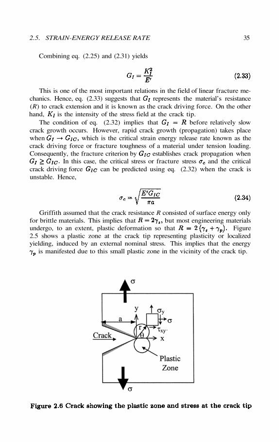
Griffith assumed that the crack resistance R consisted of surface energy onlyfor brittle materials. This implies that but most engineering materialsundergo, to an extent, plastic deformation so that Figure2.5 shows a plastic zone at the crack tip representing plasticity or localizedyielding, induced by an external nominal stress. This implies that the energy
is manifested due to this small plastic zone in the vicinity of the crack tip.
36 CHAPTER 2. INTRODUCTION TO FRACTURE MECHANICS
It is clear that the internal stresses on an element of an elastic-plastic bound-ary are induced by plasticity and are temperature-dependent tensors. The stressin front of the crack tip or within the plastic zone exceeds the local microscopicyield stress, which may be defined as the theoretical or cohesive stress for break-ing atomic bonds. If microscopic plasticity through activated slip systems doesnot occur, as in glasses, then a linear elastic fracture is achieved as the con-trolling fracture process. In essence, the fracture process is associated withplasticity at a microscopic level.
If large plasticity occurs at the crack tip, then the crack blunts and its radiusof curvature increases. This plastic deformation process is strongly dependent onthe temperature and microstructure. Regardless of the shape of the plastic zone,the irreversible crack tip plasticity is an indication of a local strain hardeningprocess during which slip systems are activated and dislocations pile up anddislocation interaction occurs.
2.6 GRAIN-SIZE REFINEMENT
In addition, the grain size refinement technique is used to enhance the strengthand fracture toughness of body-centered cubic (BCC) materials, such as lowcarbon steels. Letting a crack size be in the order of the average grain size
it can be shown that both yield strength and fracture toughnessdepend on the grain size. Using the Hall-Petch equation for and
eq. (2.34) for it is clear that these stress entities depend on the grain size.Hence,
where = Constant friction stress= Dislocation locking term= Constant
Denote that eqs. (2.35) and (2.36) predict that andThe slopes of these equations, and respectively, have the same unitsand they may be assumed to be related to fracture toughness. However, isreferred to as the dislocation locking term that restricts yielding from a grainto the adjacent one. Moreover, analysis of these equations for materials havingtemperature and grain size dependency indicate that both and
as but due to the inherent friction stress so at a temperature
Furthermore, represents the stress required for dislocation motion alongslip planes in BCC polycrystalline materials. One can observe that for
2.7. PROBLEMS 37
which means that is regarded as the yield stress of a single crystal.However, and as is an unrealistic case. Therefore,grain size refinement is a useful strengthening mechanism for increasing both
and At a temperature decreases since and alsodecrease, and increases. Therefore, must decrease.
Briefly, if a dislocation source is activated, then it causes dislocation motionto occur towards the grain boundary, which is the obstacle suitable for disloca-tion pile up. This pile up causes a stress concentration at the grain boundary,which eventually fractures when the local stress (shear stress) reaches a criticalvalue. Therefore, another dislocation sources are generated. This is a possiblemechanism for explaining the yielding phenomenon from one grain to the next.However, the grain size dictates the size of dislocation pile-up, the distance dis-locations must travel, and the dislocation density associated with yielding. Thisimplies that the finer the grains the higher the yield strength.
If a suitable volume of hard particles exists in a fine-grain material, theyield stress is enhanced further since three possible strengthening mechanismsare present. That is, solution strengthening, fine grain strengthening and par-ticle (dispersion) strengthening. If these three strengthening mechanisms areactivated, then the Hall-Petch model is not a suitable model for explaining thestrengthening process, but the material strengthening is enhanced due to thesemechanisms. This suitable explanation is vital in understanding that the grainsize plays a major role in determining material properties such as the yieldstrength and fracture toughness.
2.7 PROBLEMS
2.1 Show that the applied stress is when the crack tip radius isExplain.
2.2 In order for crack propagation to take place, the strain energy isdefined by the following inequality where is thecrack extension. Show that the crack driving force at instability is defined by
2.3 One steel strap has a 3-mm long centralcrack. This strap is loaded in tension to failure. Assume that the steel isbrittle having the following properties: E = 207 and
Determine a) the critical stress and b) the critical strain-energy release rate.
2.4 Suppose that a structure made of plates has one cracked plate. Ifthe crack reaches a critical size, will the plate fracture or the entire structurecollapse? Explain.
2.5 What is crack instability according to Griffith criterion?2.6 Assume that a quenched 1.2%C-steel plate has. a penny-shaped crack.
Will the Griffith theory be applicable to this plate?
38 CHAPTER 2. INTRODUCTION TO FRACTURE MECHANICS
2.7 Will the Irwin theory be valid for a changing plastic zone size duringcrack growth?
2.8 What are the major roles of the surface energy and the stored elasticenergy during crack growth?
2.9 What does happen to the elastic energy during crack growth?2.10 What does mean?
2.8 REFERENCES
[1] J.W. Dally and W.F. Riley, “Experimental Stress Analysis,” third edition,McGraw-Hill, Inc., New York, (1991)
[2] G.R. Irwin, “Fracture I,” in S. Flugge (ed), Handbuch der Physik VI,Springer-Verlag, New York, (1958) 558-590
[3] C.E. Inglis, “Stresses in a Plate due to the Presence of Cracks and SharpCorners,” Trans. Institute of Naval Architecture, 55 (1913) 219-241
[4] A.A. Griffith, “The Phenomena of Rupture and Flows in Solids,” Phil.Trans. Royal Soc., 221 (1921) 163-167
[5] H.M. Westergaard, “Bearing Pressures and Cracks,” Journal of AppliedMechanics, G1 (1939) A49 - A53
[6] W. J. McGregor Tegart, “Elements of Mechanical Metallurgy,” Macmil-lan, NY, (1966)
[7] A.P. Boresi and O.M. Sidebottom, “Advanced Mechanics of Materials”,John Wiley & Sons, New York, (1985) 534-538
[8] J.A. Collins, “Failure of Materials in Mechanical Design: Analysis,Prediction, Prevention,” Second Edition, John Wiley & Sons, New York (1993)422
[9] S.P. Timoshenko and J.N. Goodier, “Theory of Elasticity,” Third edi-tion, McGraw-Hill Co., New York, (1970) 193
[10] H.J. Grover, “Fatigue Aircraft Structures,” NAVIR 01-1A-13 Depart-ment of the Navy, US, (1966)
[11] D. Broek, “Elementary Engineering Fracture Mechanics,” fourth edition,Kluwer Academic Publisher, Boston, (1986)
[12] K. Hellan, “Introduction to Fracture Mechanics,” McGraw-Hill, NewYork, (1984)
[13] R.W. Hertzberg, “ Deformation and Fracture Mechanics of EngineeringMaterials,” Third edition, John Wiley & Sons, New York, (1989)
[14] J.M. Barsom and S.T. Rolfe, “Fracture and Fatigue Control in Struc-tures: Applications of Fracture Mechanics,” Third edition, American SocietyFor Testing and Materials, West Conshocken, PA, (199) Chapter 2
[15] E. Orowan, “Fatigue and Fracture of Metals,” MIT Press, Cambridge,MA, (1950) 139
Chapter 3
LINEAR ELASTICFRACTURE MECHANICS
3.1 INTRODUCTION
Solid bodies containing cracks can be characterized by defining a state of stressnear a crack tip and the energy balance coupled with fracture. Introducingthe Westergaard’s complex function and will allow the development a signifi-cant stress analysis at the crack tip. These particular functions can be foundelsewhere [1]. For instance, Irwin [2] treated the singular stress field by intro-ducing a quantity known as the stress intensity factor, which is used as thecontrolling parameter for evaluating the critical state of a crack.
The theory of linear-elastic fracture mechanics (LEFM) is integrated in thischapter using an analytical approach that will provide the reader useful ana-lytical steps. Thus, the reader will have a clear understanding of the conceptsinvolved in this particular engineering field and will develop the skills for a math-ematical background in determining the elastic stress field equations around acrack tip. The field equations are assumed to be within a small plastic zoneahead of the crack tip. If this plastic zone is sufficiently small, the small-scaleyielding approach is used for characterizing brittle solids and for determiningthe stress and strain fields when the size of the plastic zone is sufficiently smallerthan the crack length; than is, In contrast, a large-scale yielding is forductile solids, in which
Most static failure theories assume that the solid material to be analyzedis perfectly homogeneous, isotropic and free of stress risers or defects, such asvoids, cracks, inclusions and mechanical discontinuities (indentations, scratchesor gouges). Actually, fracture mechanics considers structural components hav-ing small flaws or cracks which are introduced during solidification, quenching,welding, machining or handling process. However, cracks that develop in serviceare difficult to predict and account for preventing crack growth.
40 CHAPTER 3. LINEAR ELASTIC FRACTURE MECHANICS
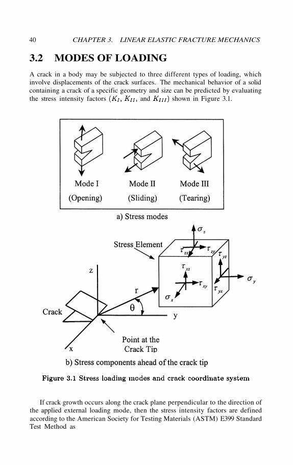
3.2 MODES OF LOADING
A crack in a body may be subjected to three different types of loading, whichinvolve displacements of the crack surfaces. The mechanical behavior of a solidcontaining a crack of a specific geometry and size can be predicted by evaluatingthe stress intensity factors and shown in Figure 3.1.
If crack growth occurs along the crack plane perpendicular to the direction ofthe applied external loading mode, then the stress intensity factors are definedaccording to the American Society for Testing Materials (ASTM) E399 StandardTest Method as
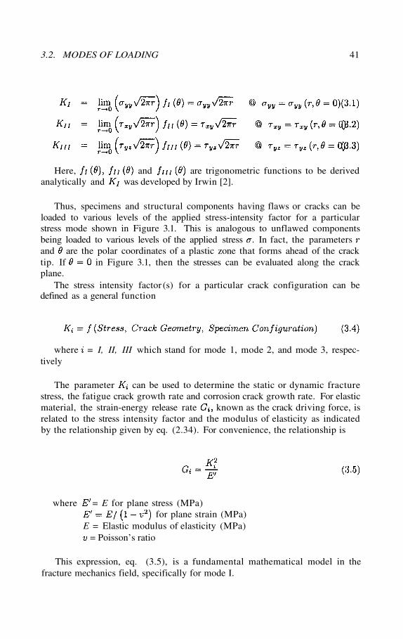
3.2. MODES OF LOADING 41
Here, and are trigonometric functions to be derivedanalytically and was developed by Irwin [2].
Thus, specimens and structural components having flaws or cracks can beloaded to various levels of the applied stress-intensity factor for a particularstress mode shown in Figure 3.1. This is analogous to unflawed componentsbeing loaded to various levels of the applied stress In fact, the parametersand are the polar coordinates of a plastic zone that forms ahead of the cracktip. If in Figure 3.1, then the stresses can be evaluated along the crackplane.
The stress intensity factor (s) for a particular crack configuration can bedefined as a general function
where = I, II, III which stand for mode 1, mode 2, and mode 3, respec-tively
The parameter can be used to determine the static or dynamic fracturestress, the fatigue crack growth rate and corrosion crack growth rate. For elasticmaterial, the strain-energy release rate known as the crack driving force, isrelated to the stress intensity factor and the modulus of elasticity as indicatedby the relationship given by eq. (2.34). For convenience, the relationship is
where = E for plane stress (MPa)for plane strain (MPa)
E = Elastic modulus of elasticity (MPa)= Poisson’s ratio
This expression, eq. (3.5), is a fundamental mathematical model in thefracture mechanics field, specifically for mode I.
42 CHAPTER 3. LINEAR ELASTIC FRACTURE MECHANICS
3.3 WESTERGAARD’S STRESS FUNCTION
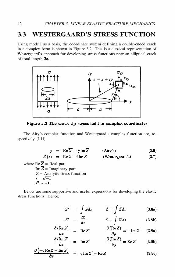
Using mode I as a basis, the coordinate system defining a double-ended crackin a complex form is shown in Figure 3.2. This is a classical representation ofWestergaard’s approach for developing stress functions near an elliptical crackof total length
The Airy’s complex function and Westergaard’s complex function are, re-spectively [1,11]
where Re = Real partIm = Imaginary partZ = Analytic stress function
Below are some supportive and useful expressions for developing the elasticstress functions. Hence,
3.3. WESTERGAARD’S STRESS FUNCTION 43
For the ellipse in Figure 3.2, the complex function and its conjugate are,respectively
and
Furthermore, the Cauchy-Riemann equations in some domain D areconsidered fundamental and sufficient for a complex function to be analytic inD. Letting then the Cauchy-Riemann important theoremstates that and so that the function beanalytic. The Cauchy-Riemann condition is of great practical importance fordetermining elastic stresses. Hence,
which must be satisfied by an Airy’s stress function. The operator inrectangular and polar coordinates takes the form
Assume that the Airy’s partial derivatives given by eq. (1.9) are applicableto elastic materials. Hence,
Thus,
44 CHAPTER 3. LINEAR ELASTIC FRACTURE MECHANICS
Substituting eq. (3.19) into eq. (3.18) along with yields the Wester-gaard’s stresses in two-dimensions
These are the stresses, eq. (3.20), that were proposed by Westergaard asthe stress singularity field at the crack tip. However, additional terms must beadded to the stress functions, eq. (3.20), analytic over an entire region, for anadequate representation of a stress field adjacent to the crack tip. This impliesthat when solving practical problems, additional boundary conditions must beimposed on the stresses. This leads to the well-known boundary value problemin which the boundary value method (BVM) is an alternative technique tothe most commonly finite element method (FEM) and finite difference method(FDM). Therefore, the original Westergaard’s stresses no longer give a uniquesolution and the analysis of the stress field in a region near the crack tip is ofextreme importance.
Consider a classical problem in fracture mechanics in which a plate con-taining an elliptical crack, as shown in Figure 3.2, is subjected to biaxial stress,
where the Westergaard’s stress function applies to thisproblem [1].
3.3.1 FAR-FIELD BOUNDARY CONDITIONS
The function Z is considered to be analytic because its derivative isdefined unambiguously and the origin is located at the center of the ellipse(Figure 3.2). Let the Westergaard’s complex function be defined by [1]
3.3. WESTERGAARD’S STRESS FUNCTION 45
However, the far-field boundary conditions require that andConsequently, eq. (3.21) becomes
from which and Substituting eq. (3.22) into (3.20)yields
On the crack surface: If y = 0 and for then Re Z = 0and Therefore, Z is not an analytical function because it doesnot have a unique derivative at a point.
3.3.2 NEAR-FIELD BOUNDARY CONDITIONS
Locate the origin at the crack tip in Figure 3.2 so that the Westergaard complexfunction becomes [1]
The near-field boundary conditions are near the crack tip andwhere N is a real number. Hence, eq. (3.24) becomes
from which the real and imaginary parts are extracted as
46 CHAPTER 3. LINEAR ELASTIC FRACTURE MECHANICS
The stresses, eq. (3.20), along the crack line, where and takethe form
If the plastic zone ahead of the crack tip is then the stress becomesThis stress defines what is referred to as “a singularity state of stress.”
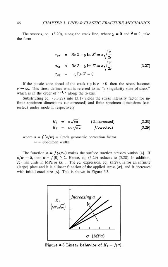
which is in the order of along the x-axis.Substituting eq. (3.3.27) into (3.1) yields the stress intensity factor for in-
finite specimen dimensions (uncorrected) and finite specimen dimensions (cor-rected) under mode I, respectively
where = Crack geometric correction factor= Specimen width
The function makes the surface traction stresses vanish [4]. Ifthen Hence, eq. (3.29) reduces to (3.28). In addition,
has units in MPa or ksi . The expression, eq. (3.28), is for an infinite(large) plate and it is a linear function of the applied stress and it increaseswith initial crack size This is shown in Figure 3.3.
3.4. SPECIMEN GEOMETRIES 47
The onset of crack propagation is a critical condition so that the crack a)extends suddenly by tearing in a shear-rupture failure or b) extends suddenlyat high velocity for cleavage fracture. All this means that the crack is unstablewhen a critical condition exists due to an applied load. In this case, the stressintensity factor reaches a critical magnitude and it is treated as a material prop-erty called fracture toughness. For sufficiently thick materials, the plane strainfracture toughness is a material property that measures crack resis-tance. Therefore, the fracture criterion by states that crack propagationoccurs when which defines a failure criterion for brittle materials.
This simply implies that the crack extends to reach a critical crack lengthdefining a critical state in which the crack speed is in the magnitude
of the speed of sound for most brittle materials. In fact, the LEFM theory iswell documented and the ASTM E399 Standard Testing Method, Vol. 03.01,validates the data and assures the minimum thickness through Brown andStrawley [27] empirical equation
3.4 SPECIMEN GEOMETRIES
In general, the successful application of linear elastic fracture mechanics to struc-tural analysis, fatigue, and stress corrosion cracking requires a known stress in-tensity factor equation for a particular specimen configuration. Cracks in bodiesof finite size are important since cracks pose a threat to the instability and safetyof an entire structure.
If mode I loading system is considered, then it is important to determinethe applied stress intensity factor and the plane strain fracture toughness
for a specific geometry in order to assess the safety factor for the crackedbody. In fact, mode I (opening) loading system is the most studied and eval-uated mode for determining the mechanical behavior of solids having specificgeometries exposed to a particular environment. Some selected and practicalcrack configurations are shown in Table 3.1.
3.4.1 THROUGH-THE-THICKNESS CENTER CRACK
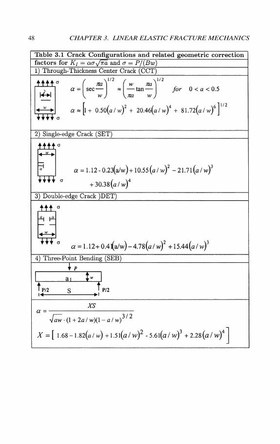
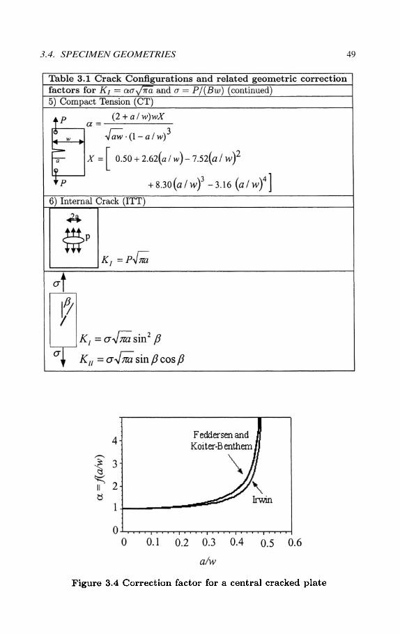
This is a commonly encountered crack configurations under a remote appliedstress as shown in Table 3.1. The geometric correction factor expression isgiven in Table 3.1 and graphically shown in Figure 3.4 as per different authorscited below. For a finite width plate, the geometric correction factor is definedby
48 CHAPTER 3. LINEAR ELASTIC FRACTURE MECHANICS
3.4. SPECIMEN GEOMETRIES 49
Example 3.1 A large plate containing a central cracklong is subjected to a tension stress as shown in the figure below. If the crackgrowth rate is 10 mm/month and fracture is expected at 10 months from now,calculate the fracture stress. Data:
Example 3.2 A large and thick plate containing a though-the-thickness cen-tral crack is 4-mm long and it fractures when a tensile stress of is ap-plied. Calculate the strain-energy release rate using a) the Griffith theory andb) the LEFM approach. Should there be a significant difference between results?Explain. Data: and
50 CHAPTER 3. LINEAR ELASTIC FRACTURE MECHANICS
Solution:If the crack growth rate is defined by
Then
Now, the fracture stress can be calculated using eq. (3.29). A large plateimplies that and from Table 3.1 the geometric correction factor becomes
Thus, the fracture stress is
Solution:The total crack size is a) Using eq. (2.35) yields
b) Using eq. (3.29) along with and gives
These results indicate that there should not be any difference because eitherapproach gives the same result.
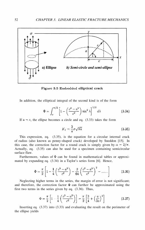
This section deals with elliptical and circular cracks. According to Irwin’s analy-sis [13] on an infinite plate containing an embedded elliptical crack (Figure 3.5)loaded in tension, the stress intensity factor is defined by
which can be evaluated at a point on the perimeter of the crack. This pointis located at an angle with respect to the direction of the applied tensile stress.
3.4. SPECIMEN GEOMETRIES 51
From eq. (2.34),
3.4.2 ELLIPTICAL CRACKS
52 CHAPTER 3. LINEAR ELASTIC FRACTURE MECHANICS
In addition, the elliptical integral of the second kind is of the form
If the ellipse becomes a circle and eq. (3.33) takes the form
This expression, eq. (3.35), is the equation for a circular internal crackof radius (also known as penny-shaped crack) developed by Sneddon [15]. Inthis case, the correction factor for a round crack is simply given byActually, eq. (3.35) can also be used for a specimen containing semicircularsurface flaw.
Furthermore, values of can be found in mathematical tables or approxi-mated by expanding eq. (3.34) in a Taylor’s series form [6]. Hence,
Neglecting higher terms in the series, the margin of error is not significant;and therefore, the correction factor can further be approximated using thefirst two terms in the series given by eq. (3.36). Thus,
Inserting eq. (3.37) into (3.33) and evaluating the result on the perimeter ofthe ellipse yields
The stress intensity factor for a plate of finite width being subjected to a uniformand remote tensile stress (mode I) is further corrected as indicated below [21,24]
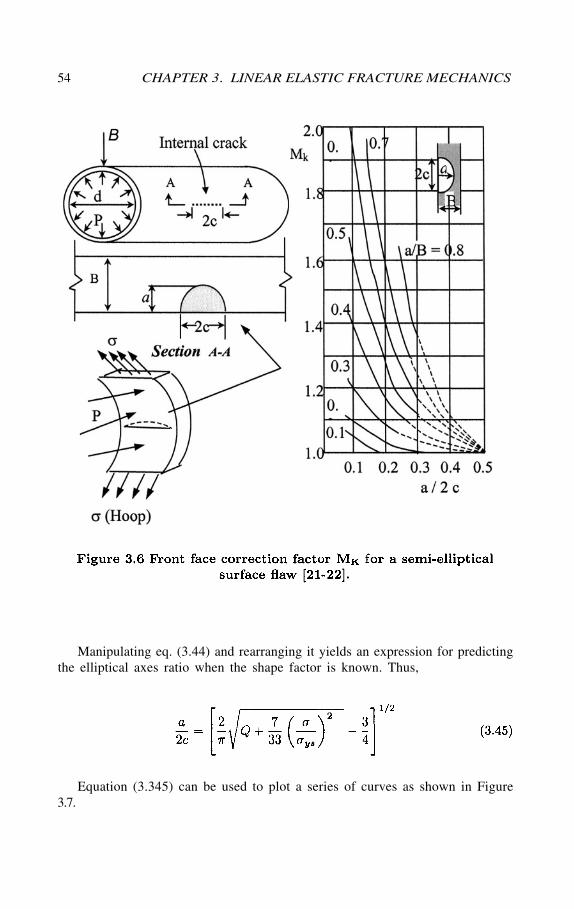
where M = Magnification correction factor= Front face correction factor [21,24] shown in Figure 3.6b
= Applied hoop stress or design stress as per Figure 3.6Q = Shape factor for a surface flaw P = Internal pressure (MPa)
Combining eqs. (3.37), (3.42) and (3.43) yields a convenient mathematicalexpression for predicting the shape factor
3.4. SPECIMEN GEOMETRIES 53
The condition is vital in evaluating elliptical crack behavior becausecan be predicted for crack instability.
3.4.3 PART-THROUGH THUMBNAIL SURFACE FLAW
54 CHAPTER 3. LINEAR ELASTIC FRACTURE MECHANICS
Manipulating eq. (3.44) and rearranging it yields an expression for predictingthe elliptical axes ratio when the shape factor is known. Thus,
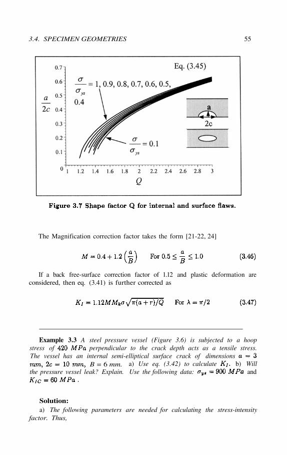
3.7.Equation (3.345) can be used to plot a series of curves as shown in Figure
3.4. SPECIMEN GEOMETRIES 55
The Magnification correction factor takes the form [21-22, 24]
If a back free-surface correction factor of 1.12 and plastic deformation areconsidered, then eq. (3.41) is further corrected as
Example 3.3 A steel pressure vessel (Figure 3.6) is subjected to a hoopstress of perpendicular to the crack depth acts as a tensile stress.The vessel has an internal semi-elliptical surface crack of dimensions
a) Use eq. (3.42) to calculate b) Willthe pressure vessel leak? Explain. Use the following data: and
Solution:a) The following parameters are needed for calculating the stress-intensity
factor. Thus,
B = 6 mm.
The plastic zone size can be determined using eq. (3.1) alongThis implies that a plastic zone develops as long as the material yields ahead ofthe crack tip. Thus,
Collecting all correction factor gives
Designing thin-wall pressure vessels to store fluids is a common practice inengineering. By definition, a thin-wall pressure vessel requires that the platethickness (B) be small as compared with the vessels internal diameter (d); thatis, or as shown in Figure 3.6. If curved plates are weldedto make pressure vessels, the welded joints become the weakest areas of thestructure since weld defects can be the source of cracks during service.
Accordingly, the internal pressure P acts in the radial direction (Figure 3.6)and the total force for rupturing the vessel on a diametral plane is where
is the projected area. Assuming that the stress across the thickness and thatthe cross-sectional area is A = 2BL, the force balance iswhich gives eq. (3.43). The hoop stress is the longitudinal stress and thetransverse stress is half the longitudinal one. These stress are principal stressesin designing against yielding. Normally, the design stress is the hoop stressdivide by a safety factor in the range of 1 < SF < 5.
For welded joints in pressure vessels, a welding efficient, canbe included in the hoop stress expression to account for weak welded joints [28].Thus, eq. (3.43) becomes
56 CHAPTER 3. LINEAR ELASTIC FRACTURE MECHANICS
b) The pressure vessel will not leak because but extreme cautionshould be taken because Thus, the safety factor is
If then leakage would occur.
3.4.4 LEAK-BEFORE-BREAK CRITERION
Let’s assume that internal surface cracks develop at welded joints or at anyother area of the vessel. In such a scenario, the leak-before-break criterion
proposed by Irwin et al. [26] can be used to predict the fracture toughness ofpressure vessels. This criterion allows an internal surface crack to grow throughthe thickness of the vessel so that for leakage to occur. This meansthat the critical crack length must be greater than the vessel thickness; that is,
Assuming a semicircular through the thickness crack the effective cracklength is defined as
The fracture toughness relationship between plane stress and plane strainconditions to establish the leak-before-break criterion may be estimated usingan empirical relationship developed by Irwin et al. [26]. Thus, the plane stressfracture toughness is and
Irwin’s expression [26] for plane stress fracture toughness is derived in Chap-ter 5 and given here for convenience. Thus,
Combining eqs. (3.48) and (3.49) along with as the critical conditionand yields the leak-before-break criterion for plane strain condition
Example 3.4 A pressure vessel made of Ti-6Al-4V alloy using a weldingfabrication technique is used in rocket motors as per Faires [28]. Helium (He)is used to provided pressure on the fuel and lox (liquid oxygen). The vesselinternal diameter and length are 0.5 m and 0.6 m, respectively, and the internalpressure is Assume a semicircular crack develops, a welding efficiencyof 100% and a safety factor of 1.6 to calculate the thickness uniform thicknessof the vessel. Use the resultant thickness to calculate the fracture toughnessaccording to eq. (3.50). Select a yield strength of
3.4. SPECIMEN GEOMETRIES 57
Use of this criterion requires that the vessel thickness meets the yieldingrequirement to withstand the internal pressure and the ASTM E399 thicknessrequirement.
Solution:
The design stress against general yielding is
From eq. (3.48),
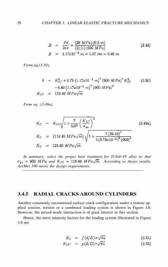
Another commonly encountered surface crack configuration under a remote ap-plied tension, torsion or a combined loading system is shown in Figure 3.8.However, the mixed-mode interaction is of great interest in this section.
Hence, the stress intensity factors for the loading system illustrated in Figure3.8 are
58 CHAPTER 3. LINEAR ELASTIC FRACTURE MECHANICS
From eq.(3.50),
From eq. (3.49a),
In summary, select the proper heat treatment for Ti-6Al-4V alloy so thatand According to theses results,
AerMet 100 meets the design requirements.
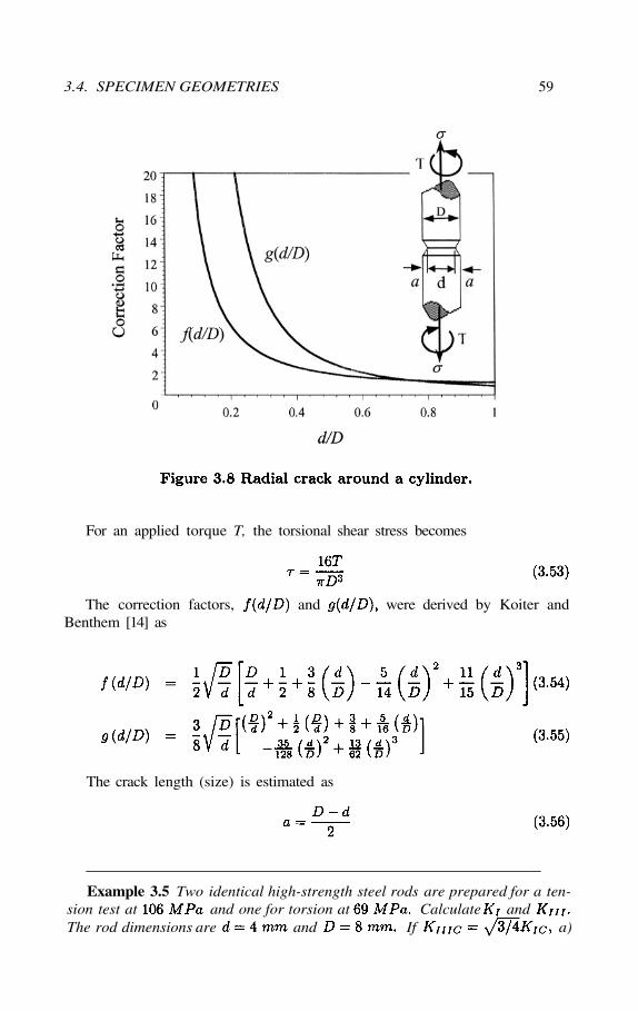
3.4.5 RADIAL CRACKS AROUND CYLINDERS
3.4. SPECIMEN GEOMETRIES 59
The correction factors, and were derived by Koiter andBenthem [14] as
The crack length (size) is estimated as
Example 3.5 Two identical high-strength steel rods are prepared for a ten-sion test at and one for torsion at Calculate andThe rod dimensions are and If a)
For an applied torque T, the torsional shear stress becomes
60 CHAPTER 3. LINEAR ELASTIC FRACTURE MECHANICS
Will the rods fracture? Explain, b) Calculate the theoretical fracture tensile andtorsion stresses if fracture does not occur in part a). Use
Solution:
a) The crack length and the radius ratios are, respectively
From eqs. (3.54) and (3.55) or Figure 3.8,
Hence, the applied stress intensity factors are calculated using eqs. (3.51)and (3.52)
Therefore, neither rod will fracture since both stress intensity factors arebelow their critical values; that is, and
b) The fracture stress are
3.5 FRACTURE CONTROL
Structures usually have inherent flaws or cracks introduced during 1) weldingprocess due to welds, embedded slag, holes, porosity, lack of fusion and 2) servicedue to fatigue, stress corrosion cracking (SCC) , impact damage and shrinkage.
A fracture-control practice is vital for design engineers in order to assure theintegrity of particular structure. This assurance can be accomplished by a closecontrol of
Given data:
and
3.5. FRACTURE CONTROL 61
1)2)3)
Design constraintsFabricationGeneral yielding
4)5)6)
MaintenanceNondestructive evaluation (NDE)Environmental effects
The pertinent details for the above elements depend on codes and proce-dures that are required by a particular organization. However, the suitabilityof a structure to brittle fracture can be evaluated using the concept of fracturemechanics, which is the main subject in this section. For instance, the elapsedtime for crack-initiation and crack-propagation determines the useful life of astructure, for which the combination of an existing crack size, applied stress,and loading rate may cause the stress intensity factor reach a critical value.
In order to describe the technical aspects of a fracture control plan, considera large plate (infinite plate) with a certain plane strain fracture toughnessso that for a stable crack. Thus, the typical design philosophy [8]uses eq. (3.28) or (3.29) as the general mathematical model in which isthe maximum allowable crack size in a component, is the design stress, andis the applied stress intensity factor. However, the minimum detectable cracksize depends on the available equipment for conducting nondestructive tests,but the critical crack size can be predicted when the stress intensity factorreaches a critical value, which is commonly known as the plane strain fracturetoughness for thick plates. In fact, can be taken asthe material fracture constraint; otherwise, the crack becomes unstable when itreaches a critical length, which is strongly controlled by Thus,solving eqs. (3.29) for the critical crack length yields
This expression implies that the maximum allowable crack length dependson the magnitude of and the applied stress Conclusively, crackpropagation occurs when the applied stress intensity factor is equal or greaterthan fracture toughness, for plane strain or for plane stresscondition.
A typical fracture-control plan includes the following
Plane strain fracture toughness, Actually, the applied stress inten-sity factor must be so that it can be used as a constraint, andthe designer controls it. This design constraint assures structural integritysince crack propagation is restricted.
Use of the following inequality for brittle materialsassures that the thickness of designed parts do not fall below a minimumthickness
If use of welding is necessary, then it must be used very cautiously since itcan degrade the toughness of the welded material especially in the heat-affected zone (HAZ), which may become brittle as a consequence of rapid
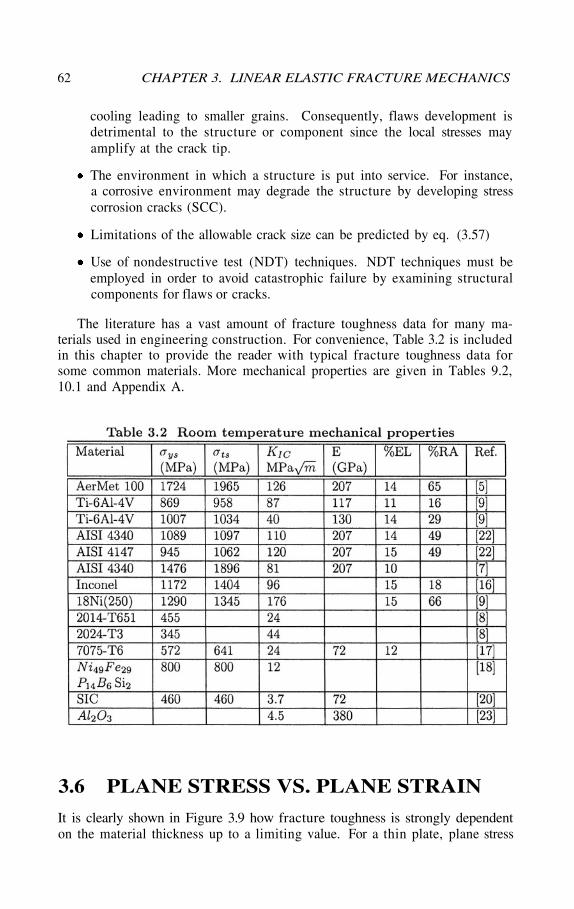
62 CHAPTER 3. LINEAR ELASTIC FRACTURE MECHANICS
cooling leading to smaller grains. Consequently, flaws development isdetrimental to the structure or component since the local stresses mayamplify at the crack tip.
The environment in which a structure is put into service. For instance,a corrosive environment may degrade the structure by developing stresscorrosion cracks (SCC).
Limitations of the allowable crack size can be predicted by eq. (3.57)
Use of nondestructive test (NDT) techniques. NDT techniques must beemployed in order to avoid catastrophic failure by examining structuralcomponents for flaws or cracks.
The literature has a vast amount of fracture toughness data for many ma-terials used in engineering construction. For convenience, Table 3.2 is includedin this chapter to provide the reader with typical fracture toughness data forsome common materials. More mechanical properties are given in Tables 9.2,10.1 and Appendix A.
3.6 PLANE STRESS VS. PLANE STRAIN
It is clearly shown in Figure 3.9 how fracture toughness is strongly dependenton the material thickness up to a limiting value. For a thin plate, plane stress
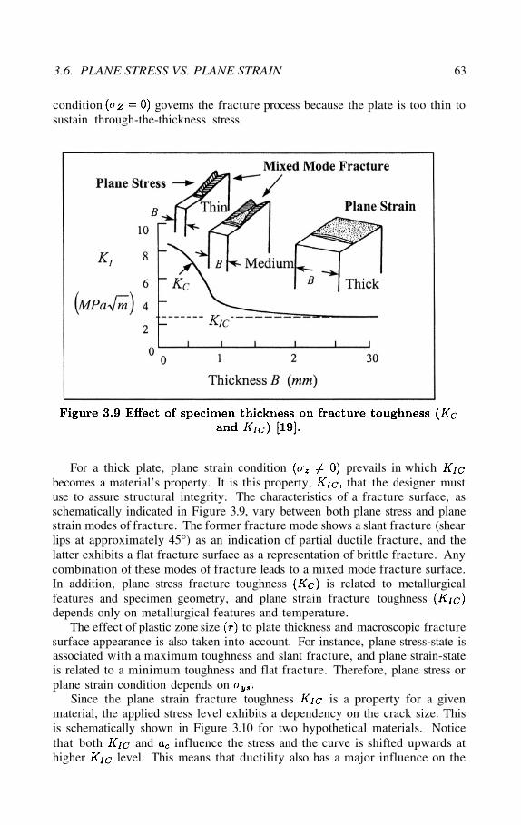
3.6. PLANE STRESS VS. PLANE STRAIN 63
condition governs the fracture process because the plate is too thin tosustain through-the-thickness stress.
For a thick plate, plane strain condition prevails in whichbecomes a material’s property. It is this property, that the designer mustuse to assure structural integrity. The characteristics of a fracture surface, asschematically indicated in Figure 3.9, vary between both plane stress and planestrain modes of fracture. The former fracture mode shows a slant fracture (shearlips at approximately 45°) as an indication of partial ductile fracture, and thelatter exhibits a flat fracture surface as a representation of brittle fracture. Anycombination of these modes of fracture leads to a mixed mode fracture surface.In addition, plane stress fracture toughness is related to metallurgicalfeatures and specimen geometry, and plane strain fracture toughnessdepends only on metallurgical features and temperature.
The effect of plastic zone size to plate thickness and macroscopic fracturesurface appearance is also taken into account. For instance, plane stress-state isassociated with a maximum toughness and slant fracture, and plane strain-stateis related to a minimum toughness and flat fracture. Therefore, plane stress orplane strain condition depends on
Since the plane strain fracture toughness is a property for a givenmaterial, the applied stress level exhibits a dependency on the crack size. Thisis schematically shown in Figure 3.10 for two hypothetical materials. Noticethat both and influence the stress and the curve is shifted upwards athigher level. This means that ductility also has a major influence on the
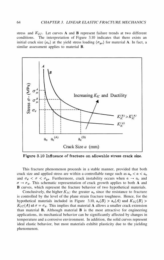
64 CHAPTER 3. LINEAR ELASTIC FRACTURE MECHANICS
stress and Let curves A and B represent failure trends at two differentconditions. The interpretation of Figure 3.10 indicates that there exists aninitial crack size at the yield stress loading for material A. In fact, asimilar assessment applies to material B.
This fracture phenomenon proceeds in a stable manner, provided that bothcrack size and applied stress are within a controllable range such asand Furthermore, crack instability occurs when and
This schematic representation of crack growth applies to both A andB curves, which represent the fracture behavior of two hypothetical materials.
Conclusively, the higher the greater since the resistance to fractureis controlled by the level of the plane strain fracture toughness. Hence, for thehypothetical materials included in Figure 3.10,
This implies that material A allows a smaller crack extensionthan material B. Although material B is the most attractive for engineeringapplications, its mechanical behavior can be significantly affected by changes intemperature and a corrosive environment. In addition, the solid curves representideal elastic behavior, but most materials exhibit plasticity due to the yieldingphenomenon.
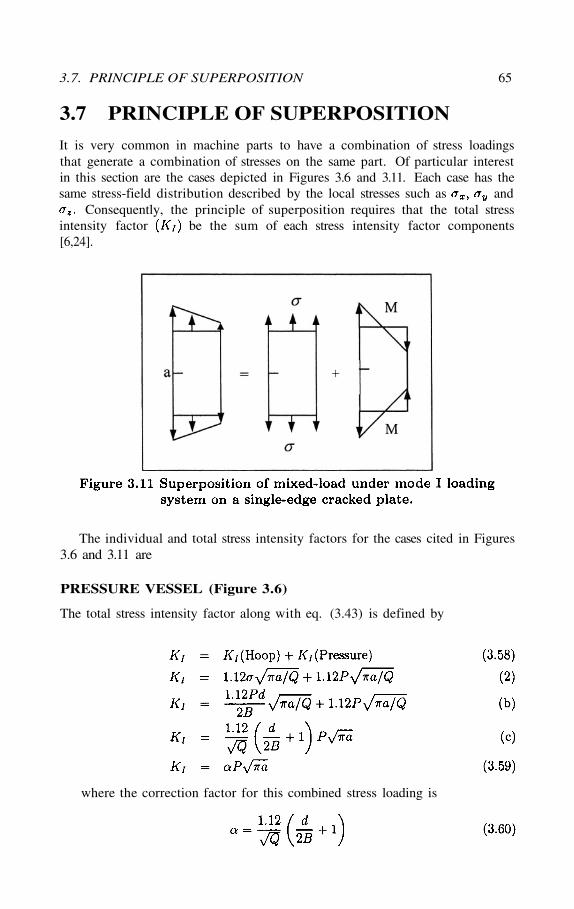
3.7. PRINCIPLE OF SUPERPOSITION 65
It is very common in machine parts to have a combination of stress loadingsthat generate a combination of stresses on the same part. Of particular interestin this section are the cases depicted in Figures 3.6 and 3.11. Each case has thesame stress-field distribution described by the local stresses such as and
Consequently, the principle of superposition requires that the total stressintensity factor be the sum of each stress intensity factor components[6,24].
3.7 PRINCIPLE OF SUPERPOSITION
The individual and total stress intensity factors for the cases cited in Figures3.6 and 3.11 are
PRESSURE VESSEL (Figure 3.6)
The total stress intensity factor along with eq. (3.43) is defined by
where the correction factor for this combined stress loading is
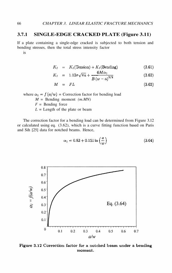
66 CHAPTER 3. LINEAR ELASTIC FRACTURE MECHANICS
If a plate containing a single-edge cracked is subjected to both tension andbending stresses, then the total stress intensity factor
is
where = Correction factor for bending loadM = Bending moment (m.MN)F = Bending forceL = Length of the plate or beam
The correction factor for a bending load can be determined from Figure 3.12or calculated using eq. (3.62), which is a curve fitting function based on Parisand Sih [25] data for notched beams. Hence,
3.7.1 SINGLE-EDGE CRACKED PLATE (Figure 3.11)
3.7. PRINCIPLE OF SUPERPOSITION 67
Example 3.6 A round vessel made of AISI 4147 is pressurized at 379 M P Aand it has an internal semi-elliptical surface crack 5-mm deep and 10-mm long.The diameter and thickness are 0.5 m and 25 cm, respectively. In order toaccount for the effects of both the applied pressure and the hoop stress, calculatea) the stress intensity factor. Will the pressure vessel fracture or leak? b)Determine the maximum pressure that would cause leakage, and c) plot thecorrection factor vs. the shape factor.
Solution:Given data: B = 25 cm,
From Table 3.2,
a) The hoop stress is
Using eq. (3.44) yields the shape factor
Using eq. (3.59) gives the total stress-intensity factor
Therefore, leakage will not occur because
c) From eq. (3.59), the maximum pressure is
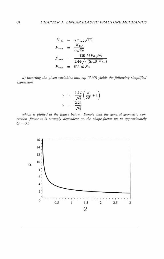
68 CHAPTER 3. LINEAR ELASTIC FRACTURE MECHANICS
d) Inserting the given variables into eq. (3.60) yields the following simplifiedexpression
which is plotted in the figure below. Denote that the general geometric cor-rection factor is strongly dependent on the shape factor up to approximatelyQ = 0.5.
3.8. PROBLEMS 69
3.8 PROBLEMS
3.1 A steel strap 1-mm thick and 20-mm wide with a through-the-thicknesscentral crack 4-mm long is loaded to failure, a) Determine the critical loadif for the strap material, b) Use an available correctionfactor, for this crack configuration and calculate the critical stressas
3.2 A steel tension bar 8-mm thick and 50-mm wide with an initial single-edge crack of 10-mm long is subjected to an uniaxial stress a)Determine the stress intensity factor Is the crack stable? b) Determinethe critical crack size, and c) determine the critical load. Data:
[Solution: a) b) 31.1 mm, and c)
3.3 A very sharp penny-shaped crack with a diameter of is com-pletely embedded in a highly brittle solid. Assume that catastrophic fractureoccurs when a stress of is applied. a) What is the fracture toughnessfor this solid? (Assume that this fracture toughness is for plane strain condi-tions). b) If a sheet 5-mm thick plate is prepared for fracture-toughness testing,Would the fracture-toughness value [(calculated in part a)] be an acceptablenumber according to the ASTM E399 standard? Use c)What thickness would be required for the fracture-toughness test to be valid?
3.4 A One guitar steel string has a miniature circumferential crack of deep. This implies that the radius ratio is almost unity, b)Another string has a localized miniature surface crack (single-edge crack like) of
deep. Assume that both strings are identical with an outer diameterof If a load of 49 N is applied to the string when being tuned, will itbreak? Given data: and
3.5 A 7075-T6 aluminum alloy is loaded in tension. Initially thethick, wide and long plate has a single-edge through–the-thickness crack. a) Is this a valid test? b) Calculate the maximum allowabletension stress this plate can support. c) Is it necessary to correct due tocrack-tip plasticity? Why? or Why not? d) Calculate the design stress and thenstress intensity factor if the safety factor is 1.5. Use the following properties:
and [Solution: a) It is a valid testbecause B(ASTM) < B(actual), b) c) It is not necessary because
and d) and
3.6 A steel plate ( thick, wide, and long) is in tension. Itis operated below its ductile-to-brittle transition temperature (with
If a long through the-thickness central crack is present,calculate a) the tensile stress for catastrophic failure. Compare this stress withthe yield strength of b) Determine the safety factor.
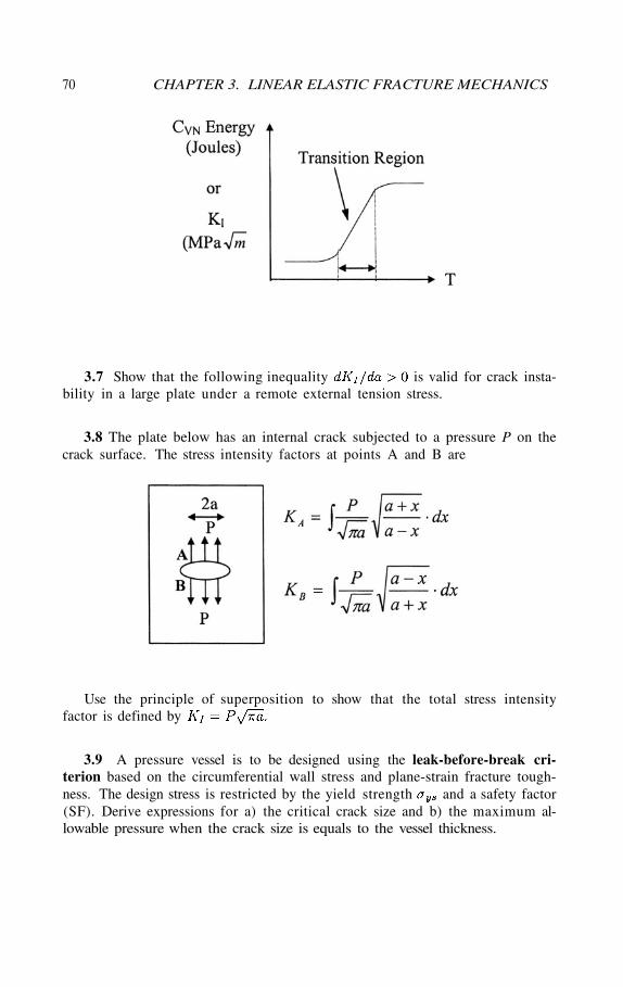
70 CHAPTER 3. LINEAR ELASTIC FRACTURE MECHANICS
3.7 Show that the following inequality is valid for crack insta-bility in a large plate under a remote external tension stress.
Use the principle of superposition to show that the total stress intensityfactor is defined by
3.9 A pressure vessel is to be designed using the leak-before-break cri-terion based on the circumferential wall stress and plane-strain fracture tough-ness. The design stress is restricted by the yield strength and a safety factor(SF). Derive expressions for a) the critical crack size and b) the maximum al-lowable pressure when the crack size is equals to the vessel thickness.
3.8 The plate below has an internal crack subjected to a pressure P on thecrack surface. The stress intensity factors at points A and B are
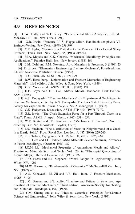
[1] J. W. Dally and W.F. Riley, “Experimental Stress Analysis”, 3rd ed.,McGraw-Hill, Inc. New York, (1991).
[2] G.R. Irwin, “Fracture I,” S. Flugge editor, Handbuch der physik VI,Springer-Verlag, New York, (1958) 558-590.
[3] C.E. Inglis, “Stresses in a Plate due to the Presence of Cracks and SharpCorners”, Trans. Inst. Nav. Arch., 55 (1913) 219-241.
[4] M.A. Meyers and K.K. Chawla, “Mechanical Metallurgy Principles andApplications,” Prentice-Hall, Inc., New Jersey, (1984) 161
[5] J.M. Dahl and P.M. Novotny, Adv. Materials & Processes, 3 (1999) 23[6] D. Broek, “Elementary Engineering Fracture Mechanics’, Fourth edition,
Kluwer Academic Publisher, Boston, (1986).[7] R.C. Shah, ASTM STP 560, (1971) 29[8] R.W. Hertz berg, “Deformation and Fracture Mechanics of Engineering
Materials”, third edition, John Wiley & Sons, New York, (1989)[9] G.R. Yoder et al., ASTM STP 801, (1983) 159.[10] H.E. Boyer And T.L. Gall, editors, Metals Handbook: Desk Edition,
ASM, (1985)[11] A.S. Kobayashi, “Fracture Mechanics”, in Experimental Techniques in
Fracture Mechanics, edited by A.S. Kobayashi, The Iowa State University Press,Society for experimental Stress Analysis, SESA monograph 1, (1973).
[12] C.E. Feddersen, Discussion, ASTM STP 410, (1967) 77-79.[13] G.R. Irwin, “The Crack Extension Force for a Part-Through Crack in a
Plate”, Trans. ASME, J. Appl. Mech., (1962) 651 - 654.[14] W.T. Koiter and J.P. Benthem, in “Mechanics of Fracture”, Vol. 1,
edited by G.C. Sih, Noordhoff, Leyden, (1973)[15] I.N. Sneddon, “The distribution of Stress in Neighborhood of a Crack
in a Elastic Solid,” Proc. Royal Soc. London, A 187 (1946) 229-260[16] R.L. Tobler, Cryogenics, Vol. 16, No. 11, (Nov. 1976) 669.[17] T.E. Tietz and I.G. Palmer, ASM Materials Science Seminar, Advances
in Power Metallurgy, (October 1981) 189[18] J.C.M. Li, “Mechanical Properties of Amorphous Metals and Alloys,”
Treatise on Materials Sci. and Tech., Vol. 20, in “Ultrarapid Quenching ofLiquid Alloys,” Herbert Herman, ed., (1981) 326
[19] H.O. Fuchs and R.I. Stephens, “Metal Fatigue in Engineering”, JohnWiley, NY, 1980
[20] M.W. Barsoum, “Fundamentals of Ceramics,” McGraw-Hill Co., Inc.,NY, (1997) 401
[21] A.S. Kobayashi, M. Zii and L.R. Hall, Inter. J. Fracture Mechanics,(1965) 81-95
[22] J.M. Barsom and S.T. Rolfe, “Fracture and Fatigue in Structure: Ap-plication of fracture Mechanics,” Third edition, American Society for Testingand Materials Philadelphia, PA, (1999).
[23] Y.M. Chiang and et al., “Physical Ceramics: Principles for CeramicScience and Engineering,” John Wiley & Sons, Inc., New York, (1997).
3.9. REFERENCES 71
3.9 REFERENCES

[24] J.M. Barsom and S.T. Rolfe, “Fracture and Fatigue Control in Struc-tures: Application of Fracture Mechanics”, Third edition, Butterworth Heine-mann, Woburn, MA, (1999).
[25] C.P. Paris and G.C. Sih, “Stress Analysis of Cracks, ASTM STP 381,(1965).
[26] G.R. Irwin, J.M. Krafft, P.C. Paris, and A.A. Wells, “Basic Concepts ofCrack Growth and Fracture,” NRL Report 6598, Naval Research Laboratory,Washington, DC, (November 21, 1967)
[27] W.F. Brown, Jr. and J.E. Strawley, ASTM STP 410, (1966)[28] V.M. Faires, “Design of Machine Elements,” The Macmillan Company,
New York, USA, (1965) 34-35
72 CHAPTER 3. LINEAR ELASTIC FRACTURE MECHANICS
Chapter 4
ELASTIC FIELDEQUATIONS
4.1 INTRODUCTIONLinear elastic fracture mechanics (LEFM) and a quasi-static load action areconsidered in this chapter in order to derive the stress, strain, and displacementfield equations adjacent to a crack tip. The field equations can be derived inseries form using rectangular and polar coordinates. Any dynamic or local un-loading is neglected in the foregoing mathematical procedures for modeling theplastic zone being as a circle with different radius It is intended henceforwardto demonstrate that the trigonometric functions and have increasingterms as the radius increases. However, the irreversible action that takes placeat the crack tip suggests that a few terms in a series expansion may be neededfor characterizing the crack tip field equations.
4.2 FIELD EQUATIONS: MODE I
The analytical approach used in this chapter is based on a very small plasticzone where higher-order terms in the plastic zone size is neglected becausethe field equations are valid and exact for Consider the small plastic zoneadjacent to the crack tip shown in Figure 4.1. Generalizing eq. (3.1) in seriesform along with yields the Westergaard’s complex functions Zand as [1]
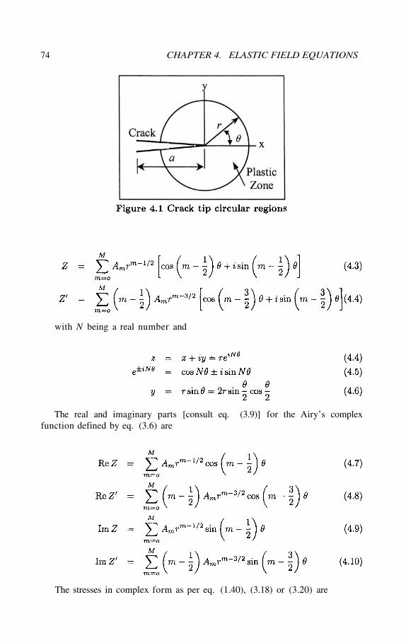
74 CHAPTER 4. ELASTIC FIELD EQUATIONS
with N being a real number and
The real and imaginary parts [consult eq. (3.9)] for the Airy’s complexfunction defined by eq. (3.6) are
The stresses in complex form as per eq. (1.40), (3.18) or (3.20) are
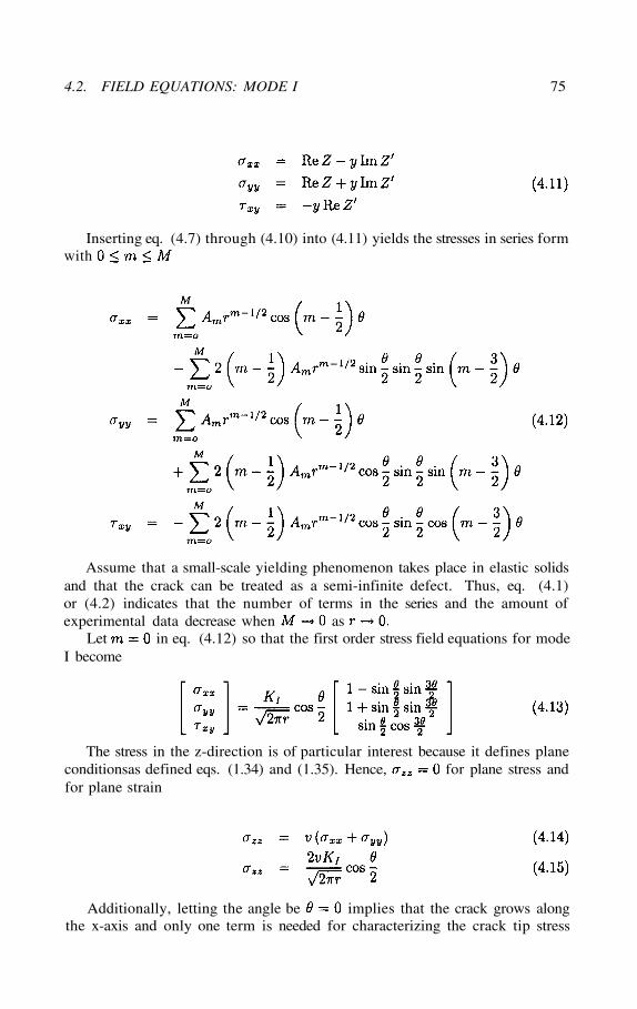
4.2. FIELD EQUATIONS: MODE I 75
Inserting eq. (4.7) through (4.10) into (4.11) yields the stresses in series formwith
Assume that a small-scale yielding phenomenon takes place in elastic solidsand that the crack can be treated as a semi-infinite defect. Thus, eq. (4.1)or (4.2) indicates that the number of terms in the series and the amount ofexperimental data decrease when as
Let in eq. (4.12) so that the first order stress field equations for modeI become
The stress in the z-direction is of particular interest because it defines planeconditionsas defined eqs. (1.34) and (1.35). Hence, for plane stress andfor plane strain
Additionally, letting the angle be implies that the crack grows alongthe x-axis and only one term is needed for characterizing the crack tip stress
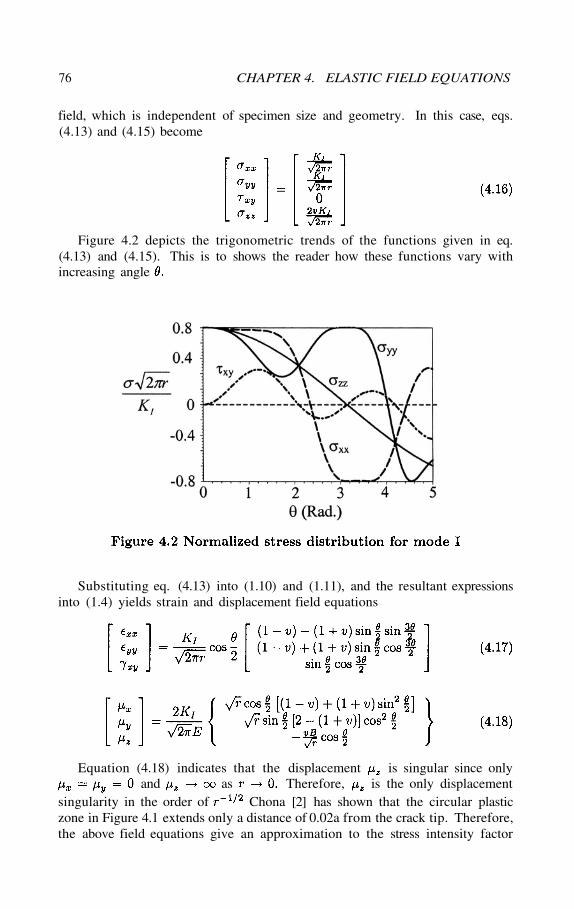
76 CHAPTER 4. ELASTIC FIELD EQUATIONS
field, which is independent of specimen size and geometry. In this case, eqs.(4.13) and (4.15) become
Figure 4.2 depicts the trigonometric trends of the functions given in eq.(4.13) and (4.15). This is to shows the reader how these functions vary withincreasing angle
Substituting eq. (4.13) into (1.10) and (1.11), and the resultant expressionsinto (1.4) yields strain and displacement field equations
Equation (4.18) indicates that the displacement is singular since onlyand as Therefore, is the only displacement
singularity in the order of Chona [2] has shown that the circular plasticzone in Figure 4.1 extends only a distance of 0.02a from the crack tip. Therefore,the above field equations give an approximation to the stress intensity factor
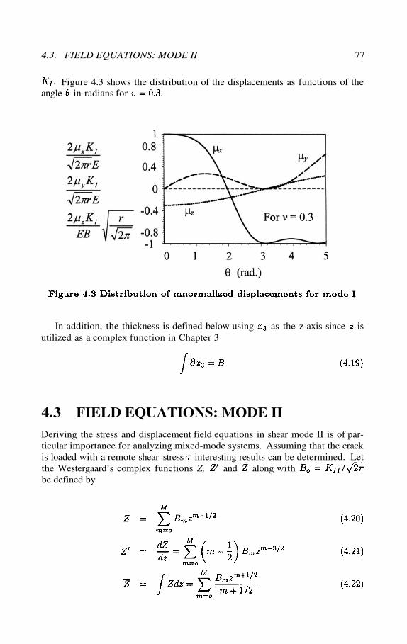
4.3. FIELD EQUATIONS: MODE II 77
Figure 4.3 shows the distribution of the displacements as functions of theangle in radians for
In addition, the thickness is defined below using as the z-axis since isutilized as a complex function in Chapter 3
4.3 FIELD EQUATIONS: MODE IIDeriving the stress and displacement field equations in shear mode II is of par-ticular importance for analyzing mixed-mode systems. Assuming that the crackis loaded with a remote shear stress interesting results can be determined. Letthe Westergaard’s complex functions Z, and along withbe defined by
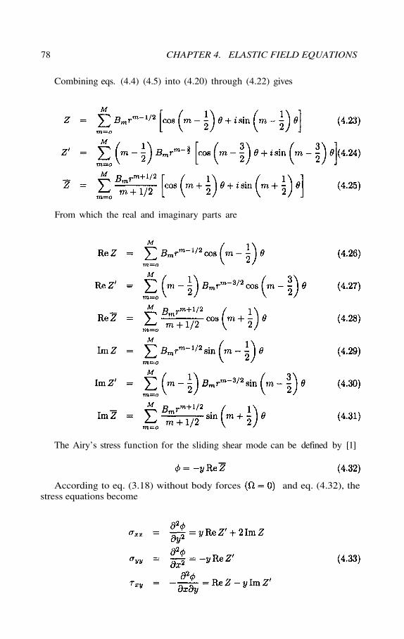
78 CHAPTER 4. ELASTIC FIELD EQUATIONS
Combining eqs. (4.4) (4.5) into (4.20) through (4.22) gives
From which the real and imaginary parts are
The Airy’s stress function for the sliding shear mode can be defined by [1]
According to eq. (3.18) without body forces and eq. (4.32), thestress equations become
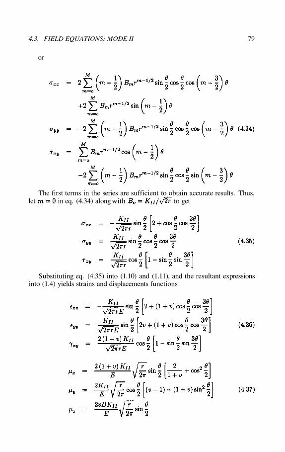
4.3. FIELD EQUATIONS: MODE II 79
or
The first terms in the series are sufficient to obtain accurate results. Thus,let in eq. (4.34) along with to get
Substituting eq. (4.35) into (1.10) and (1.11), and the resultant expressionsinto (1.4) yields strains and displacements functions
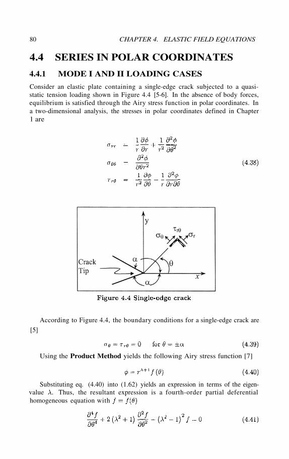
80 CHAPTER 4. ELASTIC FIELD EQUATIONS
4.4 SERIES IN POLAR COORDINATES
4.4.1 MODE I AND II LOADING CASES
Consider an elastic plate containing a single-edge crack subjected to a quasi-static tension loading shown in Figure 4.4 [5-6]. In the absence of body forces,equilibrium is satisfied through the Airy stress function in polar coordinates. Ina two-dimensional analysis, the stresses in polar coordinates defined in Chapter1 are
According to Figure 4.4, the boundary conditions for a single-edge crack are
[5]
Using the Product Method yields the following Airy stress function [7]
Substituting eq. (4.40) into (1.62) yields an expression in terms of the eigen-value Thus, the resultant expression is a fourth-order partial deferentialhomogeneous equation with
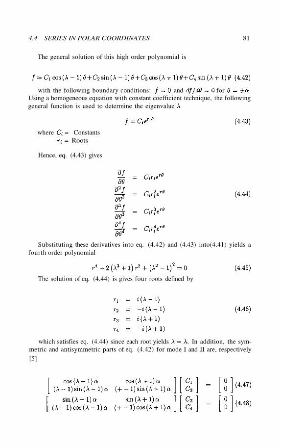
4.4. SERIES IN POLAR COORDINATES 81
The general solution of this high order polynomial is
with the following boundary conditions: and forUsing a homogeneous equation with constant coefficient technique, the followinggeneral function is used to determine the eigenvalue
where = Constants= Roots
Hence, eq. (4.43) gives
Substituting these derivatives into eq. (4.42) and (4.43) into(4.41) yields afourth order polynomial
The solution of eq. (4.44) is gives four roots defined by
which satisfies eq. (4.44) since each root yields In addition, the sym-metric and antisymmetric parts of eq. (4.42) for mode I and II are, respectively[5]
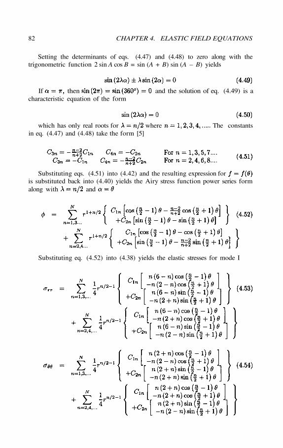
82 CHAPTER 4. ELASTIC FIELD EQUATIONS
Setting the determinants of eqs. (4.47) and (4.48) to zero along with thetrigonometric function 2 sin A cos B = sin (A + B) sin (A – B) yields
If then sin and the solution of eq. (4.49) is acharacteristic equation of the form
which has only real roots for where The constantsin eq. (4.47) and (4.48) take the form [5]
Substituting eqs. (4.51) into (4.42) and the resulting expression foris substituted back into (4.40) yields the Airy stress function power series formalong with and
Substituting eq. (4.52) into (4.38) yields the elastic stresses for mode I
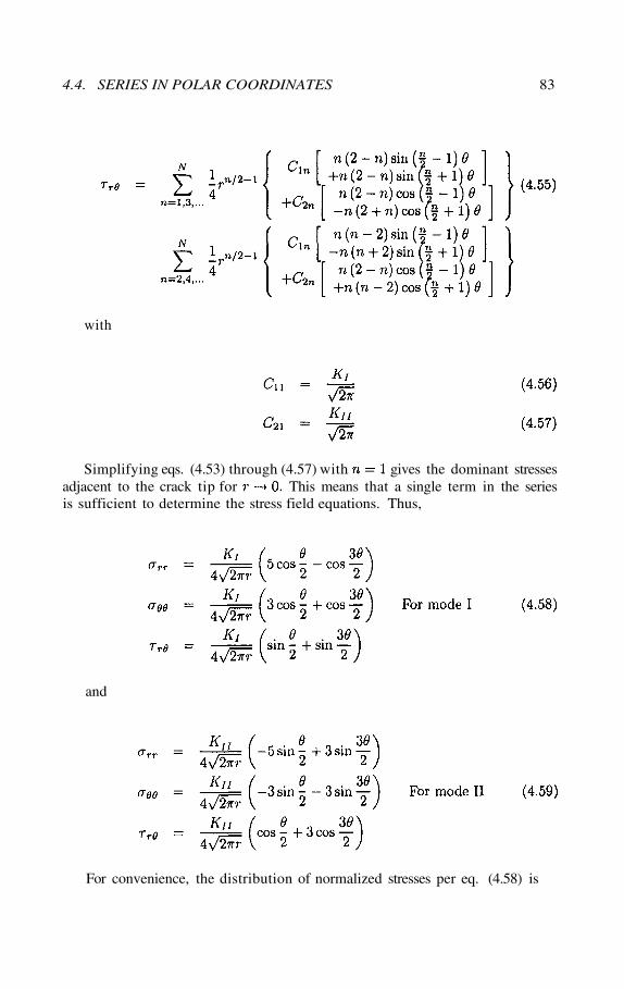
4.4. SERIES IN POLAR COORDINATES 83
with
Simplifying eqs. (4.53) through (4.57) with gives the dominant stressesadjacent to the crack tip for This means that a single term in the seriesis sufficient to determine the stress field equations. Thus,
and
For convenience, the distribution of normalized stresses per eq. (4.58) is
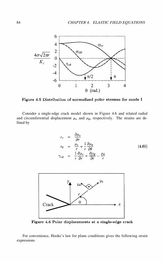
84 CHAPTER 4. ELASTIC FIELD EQUATIONS
Consider a single-edge crack model shown in Figure 4.6 and related radialand circumferential displacement and respectively. The strains are de-fined by
For convenience, Hooke’s law for plane conditions gives the following strainexpressions
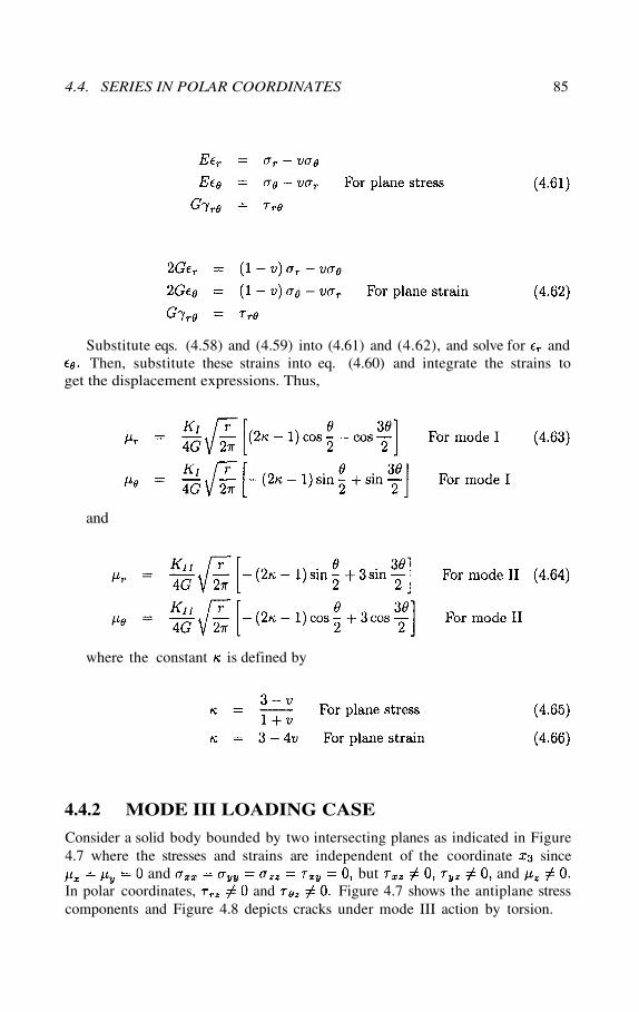
4.4. SERIES IN POLAR COORDINATES 85
Substitute eqs. (4.58) and (4.59) into (4.61) and (4.62), and solve for andThen, substitute these strains into eq. (4.60) and integrate the strains to
get the displacement expressions. Thus,
and
where the constant is defined by
4.4.2 MODE III LOADING CASE
Consider a solid body bounded by two intersecting planes as indicated in Figure4.7 where the stresses and strains are independent of the coordinate since
and but andIn polar coordinates, and Figure 4.7 shows the antiplane stresscomponents and Figure 4.8 depicts cracks under mode III action by torsion.
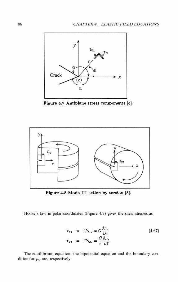
86 CHAPTER 4. ELASTIC FIELD EQUATIONS
Hooke’s law in polar coordinates (Figure 4.7) gives the shear stresses as
The equilibrium equation, the bipotential equation and the boundary con-dition for are, respectively
4.4. SERIES IN POLAR COORDINATES 87
Now assume that the out-of-plane displacement is defined by [5]
Letting and taking the derivatives needed in eq. (4.69), andsimplifying the resultant expression yields the governing second order differentialequation
The solution of eq. (4.72) can be determined by letting the function g bedefined by
Thus, eq. (4.72) yields
Inserting eq. (4.75) into (4.73) gives the characteristic equation as the so-lution of eq. (4.72) needed for determining the antisymmetric displacementwhen
Differentiating eq. (4.76) generates the boundary condition expression, whichin turn is the characteristic equation
Let in eq. (4.78) in order to simulate a crack in a solid body (Figure4.5) under mode III loading. Consequently, the eigenvalues take the form
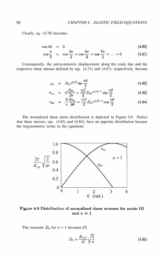
88 CHAPTER 4. ELASTIC FIELD EQUATIONS
Clearly, eq. (4.78) becomes
Consequently, the antisymmetric displacement along the crack line and therespective shear stresses defined by eqs. (4.71) and (4.67), respectively, become
The normalized shear stress distribution is depicted in Figure 4.9. Noticethat these stresses, eqs. (4.83) and (4.84), have an opposite distribution becausethe trigonometric terms in the equations
The constant for becomes [5]
4.5. HIGHER ORDER STRESS FIELD 89
The parameter in eqs. (4.82) through (4.84) corresponds to the dominantterm in the series. So far the mechanics framework for including higher orderterms in the stress series has been described for a purely linear-elastic stressfield at the crack tip. This analytical treatment allows a small plastic zoneand predicts the shear stress field. Furthermore, is the antiplane stressintensity factor. Recall that G is the shear modulus of elasticity defined by eq.(1.9).
However, the only nonzero stress is at Thus,
Thus far, the reader should have a clear understanding of the complexity offracture mechanics. For instance, the field equations being derived are for elasticmaterials so that the linear elastic fracture mechanics (LEFM) approach caneasily be applied to crack-related problems. This is a subject well documentedin the literature.
All the stress, strain and displacement field equations have the plastic zonesize in common. This implies that LEFM allows some degree of plasticityadjacent to the crack tip. However, the constraint is that the plastic zone sizemust be much smaller than the crack length; that is, otherwise, LEFMwould not be valid in solving fracture mechanics problems. If then theplastic fracture mechanics (PFM) approach becomes very useful. This subjectwill be dealt with in a later chapter.
4.5 HIGHER ORDER STRESS FIELD
The assume that the damage ahead of the crack tip is characterized by secondorder local stresses, which are dependent of specimen size and geometry asopposed to the first order terms. Consequently, the stress field are no longersingular as and the second order term in the series of expansion is knownin the literature as the T-stress for elastic behavior which accounts for effects ofstress biaxiality. Several T-stress solutions are available in the literature [8-14].
For elastic-plastic and fully plastic materials, the second order term is alsoknown as the J-Q approach [8]. In particular, O’Dowd and Shih [15-16] can beconsulted for obtaining details of the J-Q theory which describes the fundamen-tals that provide quantitative measures of the crack tip deformation. Neverthe-less, the term Q accounts for plasticity in the triaxiality state crack tip stressfield.
Considering a mixed mode fracture process and the effects of the T-stress incracked bodies, the asymptotic stress state at the crack tip can be determined by
90 CHAPTER 4. ELASTIC FIELD EQUATIONS
adding eqs. (4.13) and (4.35) and T-stress. Thus, for mode I and II interactionthe stresses are
With regard to the T-stress theory, Larsson and Carlsson [17] and Sherry etal. [18] defined as the non-singular stress that acts in the direction parallelto the crack plane and it is given as [19]
For the stress state eq. (4.89) becomes
and for pure mode I loading, T-stress becomes
In fact, this equation is the modified stress function in eq. (4.13). More-over, Leevers and Radon [20] defined to be independent of the stress intensityfactor as
where = Remote applied stress
Similarly, for pure mode II, the T-stress is [14]
In addition, in eq. (4.93) is the dimensionless stress biaxiality ratio givenas [20]
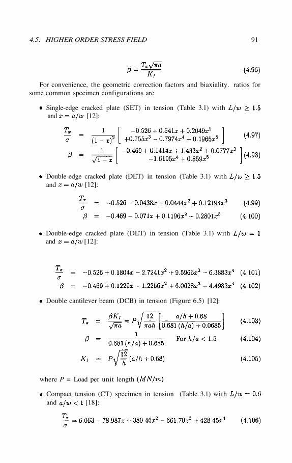
4.5. HIGHER ORDER STRESS FIELD 91
For convenience, the geometric correction factors and biaxiality. ratios forsome common specimen configurations are
Single-edge cracked plate (SET) in tension (Table 3.1) withand [12]:
Double-edge cracked plate (DET) in tension (Table 3.1) withand [12]:
Double-edge cracked plate (DET) in tension (Table 3.1) withand [12]:
Double cantilever beam (DCB) in tension (Figure 6.5) [12]:
where P = Load per unit length
Compact tension (CT) specimen in tension (Table 3.1) withand [18]:
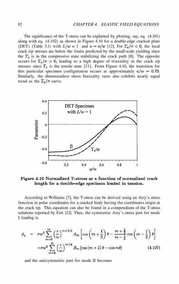
92 CHAPTER 4. ELASTIC FIELD EQUATIONS
The significance of the T-stress can be explained by plotting, say, eq. (4.101)along with eq. (4.102) as shown in Figure 4.10 for a double-edge cracked plate(DET) (Table 3.1) with and [12]. For the localcrack tip stresses are below the limits predicted by the small-scale yielding sincethe is in the compressive state stabilizing the crack path [8]. The oppositeoccurs for leading to a high degree of triaxiality in the crack tipstresses since is the tensile state [21]. From Figure 4.10, the transition forthis particular specimen configuration occurs at approximatelySimilarly, the dimensionless stress biaxiality ratio also exhibits nearly equaltrend as the curve.
According to Williams [7], the T-stress can be derived using an Airy’s stressfunction in polar coordinates for a cracked body having the coordinates origin atthe crack tip. This equation can also be found in a compendium of the T-stresssolutions reported by Fett [12]. Thus, the symmetric Airy’s stress part for modeI loading is
and the antisymmetric part for mode II becomes
4.6. REFERENCES 93
where is the characteristic dimension. According to Fett [12], eq. (4.107)can be used to determine the T-stress as
Here, is the stress contribution in the uncracked body. Further detailson this topic can be found elsewhere [12,19,21].
4.6 REFERENCES
[1] J. W. Dally and W.F. Riley, “Experimental Stress Analysis,” Third Edition,McGraw-Hill, Inc. New York, (1991)
[2] R. Chona, “Non-singular stress effects in fracture test specimens: APhotoelastic study,” M.S. thesis, University of Maryland, College Park, (August1985)
[3] G.R. Irwin, Proc. SESA, Vol. XVI, No. 1 (1958) 93-96[4] R.J. Sanford, “A critical re-examination of the Westergaard Method
for Solving Opening-Mode Crack problems,” Mech. Res., Vol. 6, No. 5, (1979)289-294
[5] K. Hellan, “Introduction to Fracture Mechanics,” McGraw-Hill Bookcompany, New York, (1984)
[6] M.H. Aliabadi and D.P. Rooke, “Numerical Fracture Mechanics,” Com-putational Mechanics Publications, Kluwer Academic Publishers, Boston, (1992)Chapter 2.
[7] M.L. Williams, “On The Stress Distribution At The Base Of A Station-ary Crack,” J. Appl. Mech., 24 (1957) 109-114
[8] T.L. Becker Jr., R.M. Cannon and R.O. Ritchie, “Finite Crack Kinkingand T-stresses in Functionally Graded Materials,” Inter. Journal of Solids andStructures, 38 (2001) 5545-5563
[9] T. Fett, “Stress Intensity Factors and T-stress For Single and Double-Edge Cracked Circular Disks Under Mixed Boundary Conditions,” Eng. Fract.Mech., Vol. 69, No. 1, (2002) 69-83
[10] T. Fett, D. Munz and G. Thun “Fracture Toughness Testing on BarsUnder Opposite Cylinder Loading,” ASME, Inter. Gas Turbine and Institute,Turbo Expo IGTI, Vol. 4A, (2002) 97-102

94 CHAPTER 4. ELASTIC FIELD EQUATIONS
[11] T. Fett, “Stress Intensity Factors and T-stress For Internally CrackedCircular Disks Under Various Boundary Conditions,” Eng. Fract. Mech., Vol.68, No. 9, (2001) 1119-1136
[12] T. Fett, “A Compendium of T-stress Solutions,” ForschungszentrumKarlsruhe, Technik and Umwelt, Wissenschaftliche Berichte, FZKA 6057,
www.ubka.uni-karlsruhe.de, (1998) 1-72[13] T. Fett, “Stress Intensity Factors and T-stress for Cracked Circular
Disks,” Forschungszentrum Karlsruhe, Technik and Umwelt, WissenschaftlicheBerichte, FZKA 6484, www.ubka.uni-karlsruhe.de, (2000) 1-68
[14] B. Chen, “The Effect of the T-stress on Crack Path Selection in Adhe-sively Bonded Joints,” Inter. Journal of Adhesion and Adhesives, Vol 21, No.5, (2001) 357-368
[15] N.P. O’Dowd and C.F. Shih, “Family of Crack-Tip Fields Characterizedby a Triaxiality Parameter: I Structure of Fields,” J. Mechanics and Physics ofSolids, Vol. 39, (1991) 989-1015
[16] N.P. O’Dowd and C.F. Shih, “Family of Crack-Tip Fields Characterizedby a Triaxiality Parameter: II Fracture Applications,” J, Mechanics and Physicsof Solids, Vol. 40, (1992) 939-963
[17] S.G. Larsson and A.J. Carlsson, “Influence of Non-Singular Stress Termsand Specimen Geometry on Small-Scale Yielding at Crack Tips in Elastic-PlasticMaterials,” J. Mechanics and Physics of Solids, Vol. 21, (1973) 263-277
[18] A.H. Sherry, C.C. France and L. Edwards, “Compendium of T-StressSolutions for Two and Three Dimensional Cracked Geometries,” The Inter.Journal, Vol. 18, (1995) 141-155
[19] A. Saxena, “Nonlinear Fracture Mechanics for Engineers,” CRC PressLLC, New York, (1998) 126,.221
[20] P.S. Leevers and J.C. Radon, “Inherent Biaxiality. in Various FractureSpecimen Geometries,” Inter. Journal, Vol. 19, (1982) 311-325
[21] M.T. Kirk, R.H. Dodds Jr,.and T.L. Anderson, “An Application Tech-nique for Predicting Size Effects on Cleavage Fracture Toughness UsingElastic T-stress,” in Fracture Mechanics, Vol. 24, ASTM STP 1207, (1994)62-86
CRACK TIP PLASTICITY
In this chapter, a few models of the configuration or the shape of the crack tipplasticity are included. It is essential to have a thorough knowledge of the shapeand size of the plastic zone in order to compare theoretical and experimentalresults for plane stress and plane strain conditions. Furthermore, the formationof the plastic zone depends on the material properties, specimen or structuralelement configuration, and loading conditions.
Most solid materials develop plastic strains when the yield strength is ex-ceeded in the region near a crack tip. Thus, the amount of plastic deformationis restricted by the surrounding material, which remains elastic during loading.
Theoretically, linear elastic stress analysis of sharp cracks predicts infinitestresses at the crack tip. In fact, inelastic deformation, such as plasticity inmetals and crazing in polymers, leads to relaxation of crack tip stresses causedby the yielding phenomenon at the crack tip. As a result, a plastic zone is formedcontaining microstructural defects such dislocations and voids. Consequently,the local stresses are limited to the yield strength of the material. This impliesthat the elastic stress analysis becomes increasingly inaccurate as the inelasticregion at the crack tip becomes sufficiently large and linear elastic fracturemechanics (LEFM) is no longer useful for predicting the field equations.
The size of the plastic zone can be estimated when moderate crack tip yield-ing occurs. Thus, the introduction of the plastic zone size as a correction pa-rameter that accounts for plasticity effects adjacent to the crack tip is vital indetermining the effective stress intensity factor or a corrected stress inten-sity factor. The plastic zone is also determined for plane conditions; that is,plane strain for maximum constraint on relatively thick components and planestress for variable constraint due to thickness effects of thin solid bodies. More-over, the plastic zone develops in most common in materials subjected to anincrease in the tensile stress that causes local yielding at the crack tip.
Chapter 5
5.1 INTRODUCTION
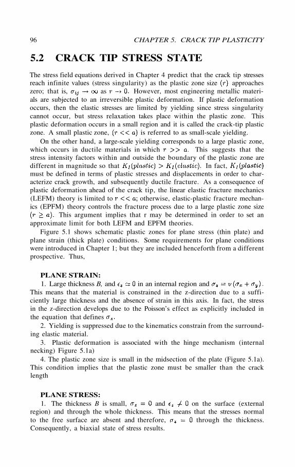
The stress field equations derived in Chapter 4 predict that the crack tip stressesreach infinite values (stress singularity) as the plastic zone size approacheszero; that is, as However, most engineering metallic materi-als are subjected to an irreversible plastic deformation. If plastic deformationoccurs, then the elastic stresses are limited by yielding since stress singularitycannot occur, but stress relaxation takes place within the plastic zone. Thisplastic deformation occurs in a small region and it is called the crack-tip plasticzone. A small plastic zone, is referred to as small-scale yielding.
On the other hand, a large-scale yielding corresponds to a large plastic zone,which occurs in ductile materials in which This suggests that thestress intensity factors within and outside the boundary of the plastic zone aredifferent in magnitude so that In fact,must be defined in terms of plastic stresses and displacements in order to char-acterize crack growth, and subsequently ductile fracture. As a consequence ofplastic deformation ahead of the crack tip, the linear elastic fracture mechanics(LEFM) theory is limited to otherwise, elastic-plastic fracture mechan-ics (EPFM) theory controls the fracture process due to a large plastic zone size
This argument implies that r may be determined in order to set anapproximate limit for both LEFM and EPFM theories.
Figure 5.1 shows schematic plastic zones for plane stress (thin plate) andplane strain (thick plate) conditions. Some requirements for plane conditionswere introduced in Chapter 1; but they are included henceforth from a differentprospective. Thus,
96 CHAPTER 5. CRACK TIP PLASTICITY
5.2 CRACK TIP STRESS STATE
PLANE STRESS:1. The thickness B is small, and on the surface (external
region) and through the whole thickness. This means that the stresses normalto the free surface are absent and therefore, through the thickness.Consequently, a biaxial state of stress results.
PLANE STRAIN:1. Large thickness B, and in an internal region and
This means that the material is constrained in the z-direction due to a suffi-ciently large thickness and the absence of strain in this axis. In fact, the stressin the z-direction develops due to the Poisson’s effect as explicitly included inthe equation that defines
2. Yielding is suppressed due to the kinematics constrain from the surround-ing elastic material.
3. Plastic deformation is associated with the hinge mechanism (internalnecking) Figure 5.1a)
4. The plastic zone size is small in the midsection of the plate (Figure 5.1a).This condition implies that the plastic zone must be smaller than the cracklength
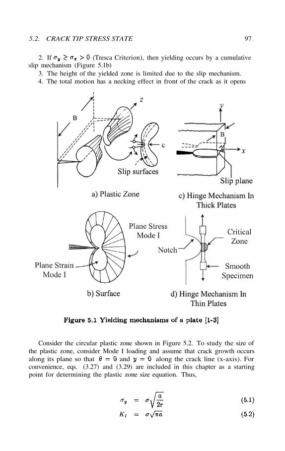
5.2. CRACK TIP STRESS STATE 97
2. If (Tresca Criterion), then yielding occurs by a cumulativeslip mechanism (Figure 5.1b)
3. The height of the yielded zone is limited due to the slip mechanism.4. The total motion has a necking effect in front of the crack as it opens
Consider the circular plastic zone shown in Figure 5.2. To study the size ofthe plastic zone, consider Mode I loading and assume that crack growth occursalong its plane so that and along the crack line (x-axis). Forconvenience, eqs. (3.27) and (3.29) are included in this chapter as a startingpoint for determining the plastic zone size equation. Thus,
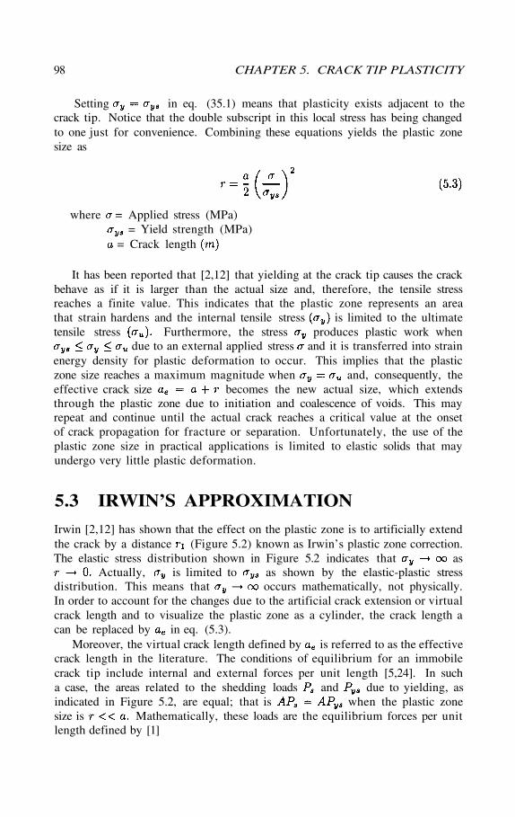
Irwin [2,12] has shown that the effect on the plastic zone is to artificially extendthe crack by a distance (Figure 5.2) known as Irwin’s plastic zone correction.The elastic stress distribution shown in Figure 5.2 indicates that as
Actually, is limited to as shown by the elastic-plastic stressdistribution. This means that occurs mathematically, not physically.In order to account for the changes due to the artificial crack extension or virtualcrack length and to visualize the plastic zone as a cylinder, the crack length acan be replaced by in eq. (5.3).
Moreover, the virtual crack length defined by is referred to as the effectivecrack length in the literature. The conditions of equilibrium for an immobilecrack tip include internal and external forces per unit length [5,24]. In sucha case, the areas related to the shedding loads and due to yielding, asindicated in Figure 5.2, are equal; that is when the plastic zonesize is Mathematically, these loads are the equilibrium forces per unitlength defined by [1]
98 CHAPTER 5. CRACK TIP PLASTICITY
Setting in eq. (35.1) means that plasticity exists adjacent to thecrack tip. Notice that the double subscript in this local stress has being changedto one just for convenience. Combining these equations yields the plastic zonesize as
where = Applied stress (MPa)= Yield strength (MPa)
= Crack length
It has been reported that [2,12] that yielding at the crack tip causes the crackbehave as if it is larger than the actual size and, therefore, the tensile stressreaches a finite value. This indicates that the plastic zone represents an areathat strain hardens and the internal tensile stress is limited to the ultimatetensile stress Furthermore, the stress produces plastic work when
due to an external applied stress and it is transferred into strainenergy density for plastic deformation to occur. This implies that the plasticzone size reaches a maximum magnitude when and, consequently, theeffective crack size becomes the new actual size, which extendsthrough the plastic zone due to initiation and coalescence of voids. This mayrepeat and continue until the actual crack reaches a critical value at the onsetof crack propagation for fracture or separation. Unfortunately, the use of theplastic zone size in practical applications is limited to elastic solids that mayundergo very little plastic deformation.
5.3 IRWIN’S APPROXIMATION
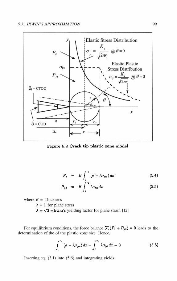
5.3. IRWIN’S APPROXIMATION 99
where B = Thickness= 1 for plane stress
yielding factor for plane strain [12]
For equilibrium conditions, the force balance leads to thedetermination of the of the plastic zone size Hence,
Inserting eq. (3.1) into (5.6) and integrating yields
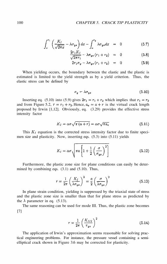
100 CHAPTER 5. CRACK TIP PLASTICITY
When yielding occurs, the boundary between the elastic and the plastic isestimated is limited to the yield strength as by a yield criterion. Thus, theelastic stress can be defined by
Inserting eq. (5.10) into (5.9) gives which implies thatand from Figure 5.2, Hence, is the virtual crack lengthproposed by Irwin [1,12]. Obviously, eq. (3.29) provides the effective stressintensity factor
This equation is the corrected stress intensity factor due to finite speci-men size and plasticity. Now, inserting eqs. (5.3) into (5.11) yields
Furthermore, the plastic zone size for plane conditions can easily be deter-mined by combining eqs. (3.1) and (5.10). Thus,
In plane strain condition, yielding is suppressed by the triaxial state of stressand the plastic zone size is smaller than that for plane stress as predicted bythe parameter in eq. (5.13).
The same reasoning can be used for mode III. Thus, the plastic zone becomes[7]
The application of Irwin’s approximation seems reasonable for solving prac-tical engineering problems. For instance, the pressure vessel containing a semi-elliptical crack shown in Figure 3.6 may be corrected for plasticity.
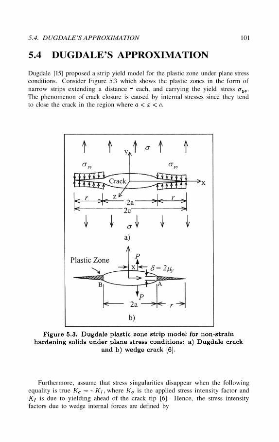
Dugdale [15] proposed a strip yield model for the plastic zone under plane stressconditions. Consider Figure 5.3 which shows the plastic zones in the form ofnarrow strips extending a distance each, and carrying the yield stressThe phenomenon of crack closure is caused by internal stresses since they tendto close the crack in the region where
Furthermore, assume that stress singularities disappear when the followingequality is true where is the applied stress intensity factor and
is due to yielding ahead of the crack tip [6]. Hence, the stress intensityfactors due to wedge internal forces are defined by
5.4. DUGDALE’S APPROXIMATION 101
5.4 DUGDALE’S APPROXIMATION
102 CHAPTER 5. CRACK TIP PLASTICITY
According to the principle of superposition, the total stress intensity factoris so that
The plastic zone correction can be accomplished by replacing the crack length for the virtual crack length and P for Thus, the stress intensity
factor are
But, and the simplified equation takes the form
Let so that
Expanding the trigonometric function eq. (5.22) yields
Neglecting the higher order terms eq. (5.22) becomes
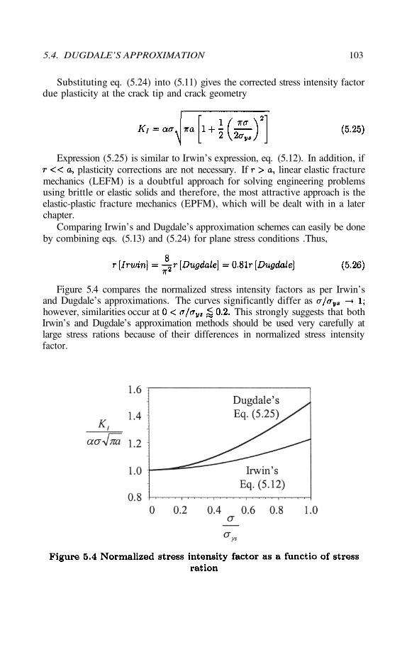
5.4. DUGDALE’S APPROXIMATION 103
Substituting eq. (5.24) into (5.11) gives the corrected stress intensity factordue plasticity at the crack tip and crack geometry
Expression (5.25) is similar to Irwin’s expression, eq. (5.12). In addition, ifplasticity corrections are not necessary. If linear elastic fracture
mechanics (LEFM) is a doubtful approach for solving engineering problemsusing brittle or elastic solids and therefore, the most attractive approach is theelastic-plastic fracture mechanics (EPFM), which will be dealt with in a laterchapter.
Comparing Irwin’s and Dugdale’s approximation schemes can easily be doneby combining eqs. (5.13) and (5.24) for plane stress conditions .Thus,
Figure 5.4 compares the normalized stress intensity factors as per Irwin’sand Dugdale’s approximations. The curves significantly differ ashowever, similarities occur at This strongly suggests that bothIrwin’s and Dugdale’s approximation methods should be used very carefully atlarge stress rations because of their differences in normalized stress intensityfactor.

So far, the characterization of cracked brittle materials has been restricted to thelinear elastic fracture criterion, which treats localized plasticity, if formed aheadof the crack tip, as a small deformed area at a small-scale yielding. Otherwise,this criterion invalidates the applicability of analytical solutions associated witha material resistance to crack growth at a large-scale yielding. In the latter case,therefore, the physical sense of acting as the controlling fracture criticalparameter is lost, to a great extent, in spite of that may be applicablewhen
The aforementioned restriction is fundamentally and quantitatively governedby nonlinear fracture mechanics through models, such as the crack tip openingdisplacement and the J-integral (J-model). The latter model treatsthe presence of large deformations as an integral part of analytical formula-tions that comprehensively describe the state of plastic stresses and strains[19-20]. Moreover, linear elastic fracture mechanics (ELFM) restricts the useof the elastic-plastic materials due to the formation of large plastic zones andnonlinear plastic behavior. Furthermore, the crack tip opening displacement
is a measure of fracture toughness of solid materials that undergoductile-to-brittle transition [26] and elastic-plastic or fully plastic behavior asin large structures (ships, pressure vessels). Subsequently, the critical stressand crack size might be predicted using this technique, provided that a criticalvalue of CTOD is known. Wells [29-30] first proposed this as a frac-ture criterion by CTOD The meaningful magnitude of dc is simplya measure of fracture toughness of ductile and thin materials.
According to the ASTM E1290 Standard [26], is used when the re-quirements are not met. Figure 5.3 shows the Dugdale’s model [15] for a centralcrack containing yielding as confined and localized narrow plastic zones in a thinsheet. This model, as depicted in Figure 5.3 simply shows the effect of yieldingon the crack length. Thus, the virtual crack size (artificial or effective cracksize) is but the plastic zone restrains crack growth (also referredto as crack extension) as the applied stress is increased. Consequently, theplastic zone reaches a critical size and crack growth occurs since lo-calized plasticity imparts an increase in dislocation density, formation of voids,and void coalescence, which act as micro-cracks within the plastic zone volumeahead of the main crack tip.
Conclusively, the use of a plastic correction approach is an appropriate math-ematical tool for reflecting the suitability to include crystal lattice defects, aspart of fracture at a microscopic scale, as an indirect form of adhered plasticityto the crack tips. Thus, the plastic zone correction appears to be suitable forcorrecting the crack opening displacement Indeed, there exists achoice of plastic zone model, Irwin’s and Dugdale’s for correcting the parameter
for thin sheets and elastic-plastic materials. According to the models shown inFigure 5.2 and 5.3, corresponds to the upper and lower relative displacementof the crack edges. If measurements of the crack opening displacement are madeclose enough to the crack tip, then From Figure 5.3b, is defined as
104 CHAPTER 5. CRACK TIP PLASTICITY
5.5 CRACK OPENING DISPLACEMENT
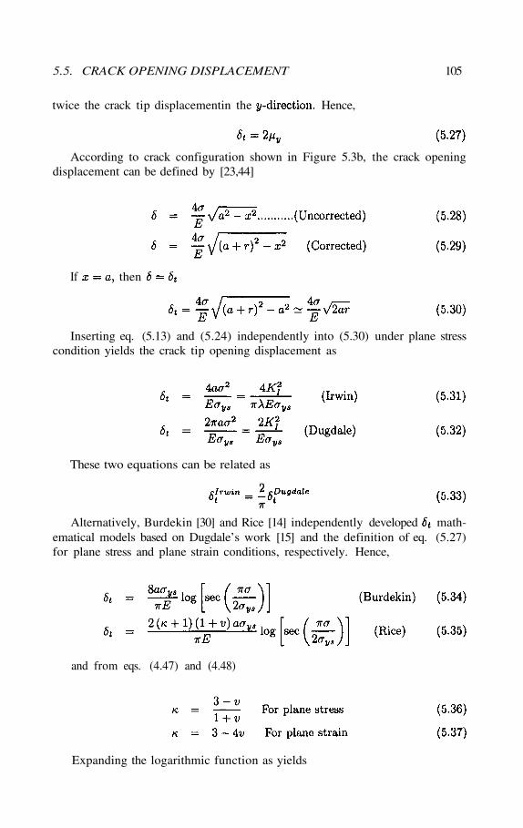
According to crack configuration shown in Figure 5.3b, the crack openingdisplacement can be defined by [23,44]
These two equations can be related as
Alternatively, Burdekin [30] and Rice [14] independently developed math-ematical models based on Dugdale’s work [15] and the definition of eq. (5.27)for plane stress and plane strain conditions, respectively. Hence,
Expanding the logarithmic function as yields
5.5. CRACK OPENING DISPLACEMENT 105
twice the crack tip displacementin the Hence,
If
Inserting eq. (5.13) and (5.24) independently into (5.30) under plane stresscondition yields the crack tip opening displacement as
and from eqs. (4.47) and (4.48)
then
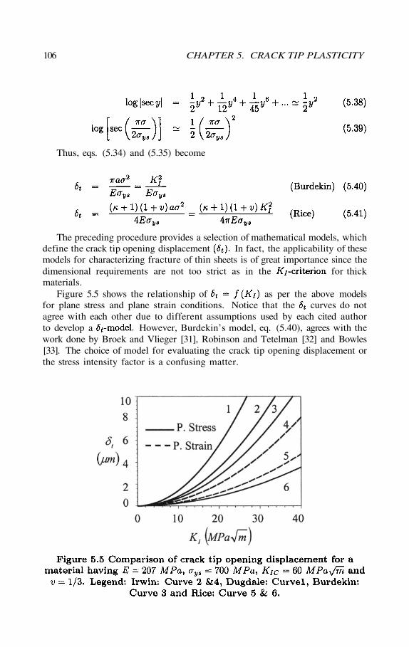
106 CHAPTER 5. CRACK TIP PLASTICITY
Thus, eqs. (5.34) and (5.35) become
The preceding procedure provides a selection of mathematical models, whichdefine the crack tip opening displacement In fact, the applicability of thesemodels for characterizing fracture of thin sheets is of great importance since thedimensional requirements are not too strict as in the for thickmaterials.
Figure 5.5 shows the relationship of as per the above modelsfor plane stress and plane strain conditions. Notice that the curves do notagree with each other due to different assumptions used by each cited authorto develop a However, Burdekin’s model, eq. (5.40), agrees with thework done by Broek and Vlieger [31], Robinson and Tetelman [32] and Bowles[33]. The choice of model for evaluating the crack tip opening displacement orthe stress intensity factor is a confusing matter.
Considerable work has been confined to the since it has the ad-vantage of measuring fracture toughness for elastic materials and it is verysensitive to variations in temperature, loading rate, specimen thickness, andthermo-mechanical processing [34].
In general, the should be confined to the yielding phenomenon ina microscopic scale, but the mathematical formulation is very complicated. Forinstance, yielding in the vicinity of a crack tip is related to complex dislocationnetworks, such as the dislocation pile-up. In this regard, reference should bemade to the classical work of Eshelby et al. [7], Stroh [8], Puttick [9], Rogers[10], Gurland et al. [11], and a review paper written by Low [13], who analyzedand studied several dislocation models for the nucleation of cracks. Therefore,the physical interpretation of the yielding phenomenon herein is confined to amacroscopic scale.
Returning to the crack tip plastic deformation in a thin sheet isnot restricted to lateral contraction which causes localized thinning at the cracktip. Thereby, crack tip blunting causes an extensive increase in the crack tipradius in the order of sheet thickness (B), and thus, the plastic zone sizemay be estimated as [15,27].
Additionally, can be related to the strain-energy release rate througheq. (3.5). For instance, combining eq. (3.5) and (5.40) at yields
So far, the extent of plastic zone has been considered along the withsince it has been modeled as a circle. However, a more accurate procedure fol-lows when so that yielding is examined in a small area modeled accordingto a particular yielding criterion, which is responsible for the theoretical shapeof the plastic zone. This fact implies that crack-tip plasticity occurs and thestresses in the zone are limited to yielding phenomenon. Therefore, the stressesare truncated to the yield stress of the material being examined and stress sin-gularity phenomenon is simply a theoretical matter. Moreover, the Von Misescriterion and Tresca Yielding Criterion may be used to derive expressions forthe plastic zone size, which in turn gives the plastic zone shape.
5.6. THE SHAPE OF THE PLASTIC ZONE 107
For plane stress condition at fracture, the strain energy release rate can beestimated as [28]
Combining eqs. (5.42) and (5.43) gives
where = Fracture strain
5.6 THE SHAPE OF THE PLASTIC ZONE
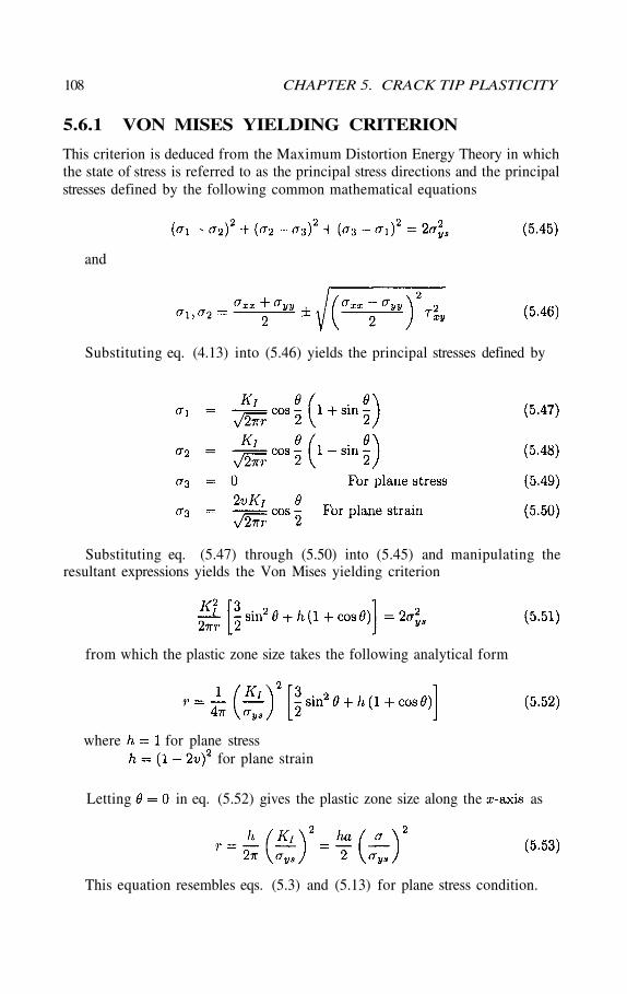
This criterion is deduced from the Maximum Distortion Energy Theory in whichthe state of stress is referred to as the principal stress directions and the principalstresses defined by the following common mathematical equations
Substituting eq. (4.13) into (5.46) yields the principal stresses defined by
108 CHAPTER 5. CRACK TIP PLASTICITY
5.6.1 VON MISES YIELDING CRITERION
and
Substituting eq. (5.47) through (5.50) into (5.45) and manipulating theresultant expressions yields the Von Mises yielding criterion
from which the plastic zone size takes the following analytical form
where for plane stressfor plane strain
Letting in eq. (5.52) gives the plastic zone size along the as
This equation resembles eqs. (5.3) and (5.13) for plane stress condition.
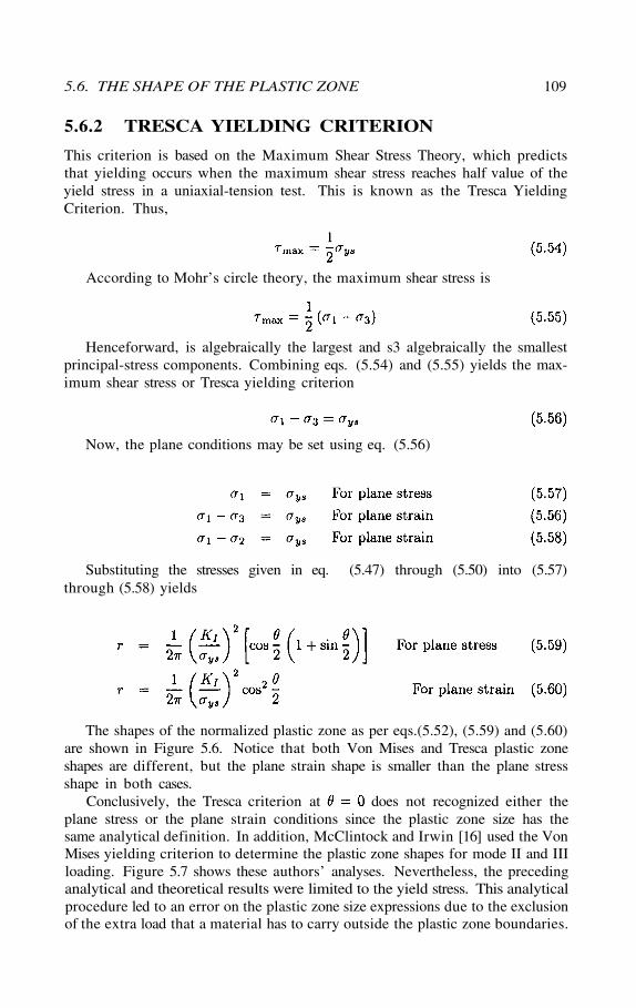
This criterion is based on the Maximum Shear Stress Theory, which predictsthat yielding occurs when the maximum shear stress reaches half value of theyield stress in a uniaxial-tension test. This is known as the Tresca YieldingCriterion. Thus,
Substituting the stresses given in eq. (5.47) through (5.50) into (5.57)through (5.58) yields
The shapes of the normalized plastic zone as per eqs.(5.52), (5.59) and (5.60)are shown in Figure 5.6. Notice that both Von Mises and Tresca plastic zoneshapes are different, but the plane strain shape is smaller than the plane stressshape in both cases.
Conclusively, the Tresca criterion at does not recognized either theplane stress or the plane strain conditions since the plastic zone size has thesame analytical definition. In addition, McClintock and Irwin [16] used the VonMises yielding criterion to determine the plastic zone shapes for mode II and IIIloading. Figure 5.7 shows these authors’ analyses. Nevertheless, the precedinganalytical and theoretical results were limited to the yield stress. This analyticalprocedure led to an error on the plastic zone size expressions due to the exclusionof the extra load that a material has to carry outside the plastic zone boundaries.
5.6. THE SHAPE OF THE PLASTIC ZONE 109
5.6.2 TRESCA YIELDING CRITERION
According to Mohr’s circle theory, the maximum shear stress is
Henceforward, is algebraically the largest and s3 algebraically the smallestprincipal-stress components. Combining eqs. (5.54) and (5.55) yields the max-imum shear stress or Tresca yielding criterion
Now, the plane conditions may be set using eq. (5.56)
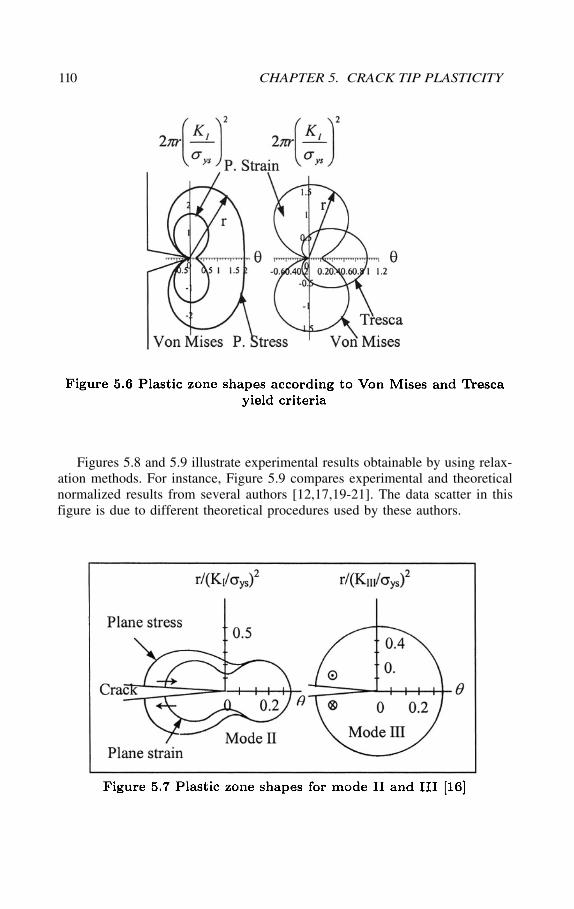
110 CHAPTER 5. CRACK TIP PLASTICITY
Figures 5.8 and 5.9 illustrate experimental results obtainable by using relax-ation methods. For instance, Figure 5.9 compares experimental and theoreticalnormalized results from several authors [12,17,19-21]. The data scatter in thisfigure is due to different theoretical procedures used by these authors.
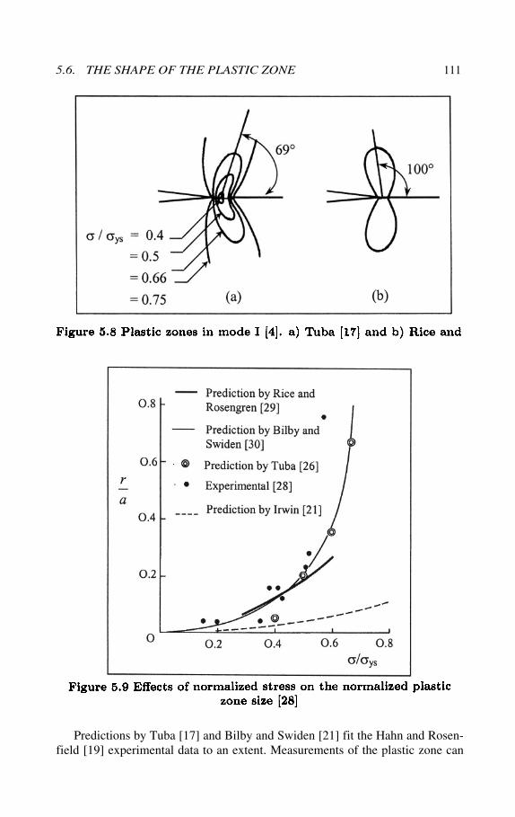
5.6. THE SHAPE OF THE PLASTIC ZONE 111
Predictions by Tuba [17] and Bilby and Swiden [21] fit the Hahn and Rosen-field [19] experimental data to an extent. Measurements of the plastic zone can
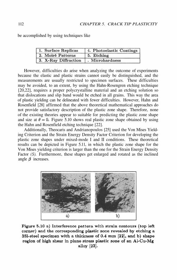
112 CHAPTER 5. CRACK TIP PLASTICITY
be accomplished by using techniques like
However, difficulties do arise when analyzing the outcome of experimentsbecause the elastic and plastic strains cannot easily be distinguished, and themeasurements are usually restricted to specimen surfaces. These difficultiesmay be avoided, to an extent, by using the Hahn-Rosengren etching technique[20,22], requires a proper polycrystalline material and an etching solution sothat dislocations and slip band would be etched in all grains. This way the areaof plastic yielding can be delineated with fewer difficulties. However, Hahn andRosenfield [28] affirmed that the above theoretical mathematical approaches donot provide satisfactory description of the plastic zone shape. Therefore, noneof the existing theories appear to suitable for predicting the plastic zone shapeand size at Figure 5.10 shows real plastic zone shape obtained by usingthe Hahn and Rosenfield etching technique [22].
Additionally, Theocaris and Andrianopoulos [25] used the Von Mises Yield-ing Criterion and the Strain Energy Density Factor Criterion for developing theplastic zone shapes under mixed-mode I and II conditions. These theoreticalresults can be depicted in Figure 5.11, in which the plastic zone shape for theVon Mises yielding criterion is larger than the one for the Strain Energy DensityFactor (S). Furthermore, these shapes get enlarged and rotated as the inclinedangle increases.
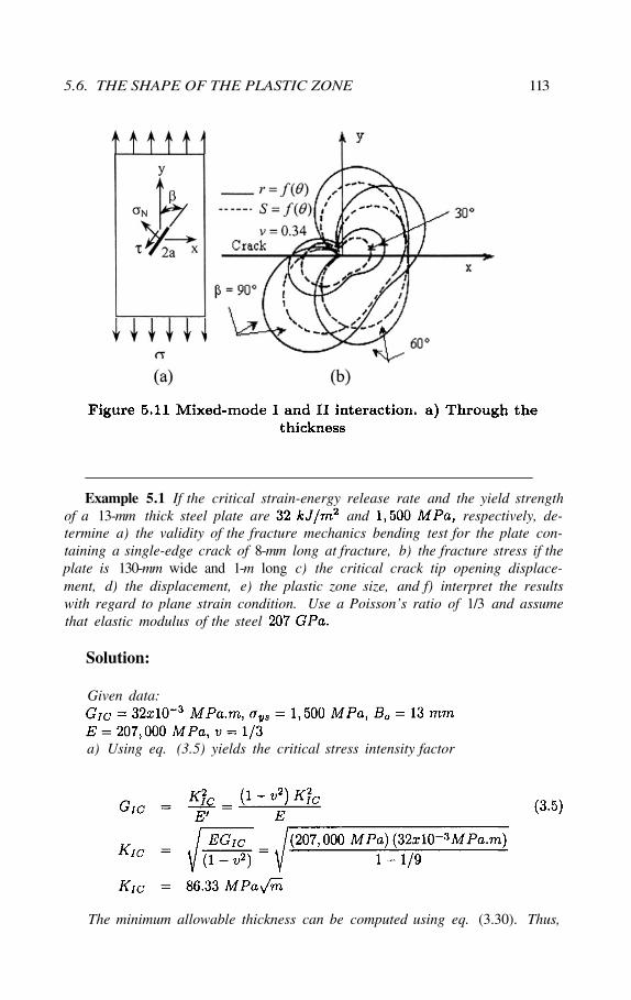
5.6. THE SHAPE OF THE PLASTIC ZONE 113
Example 5.1 If the critical strain-energy release rate and the yield strengthof a 13-mm thick steel plate are and respectively, de-termine a) the validity of the fracture mechanics bending test for the plate con-taining a single-edge crack of 8-mm long at fracture, b) the fracture stress if theplate is 130-mm wide and 1-m long c) the critical crack tip opening displace-ment, d) the displacement, e) the plastic zone size, and f) interpret the resultswith regard to plane strain condition. Use a Poisson’s ratio of 1/3 and assumethat elastic modulus of the steel
The minimum allowable thickness can be computed using eq. (3.30). Thus,
Solution:
Given data:
a) Using eq. (3.5) yields the critical stress intensity factor
114 CHAPTER 5. CRACK TIP PLASTICITY
Therefore, the test is valid because the actual specimen thickness is greaterthan the ASTM minimum thickness; that is,
b) The fracture stress is determined from eq. (3.29) along withsince (Consult Table 3.1).
c) The crack tip opening displacement is calculated using Rice’s equationwith and
d) The displacement is
e) The plastic zone can be calculated using eq. (5.53) along with
f) The above results suggests that the plate met the ASTM E399 thicknessrequirements because and behaved in a brittle manner because boththe plastic zone size and the crack tip opening displacement are very small.
Example 5.2 A thin steel plate having a 8 mm through the thickness single-edge crack size is designed to hold a static tension load. The steel prop-erties are and The plate isL = 4-m long, 60-mm wide and 3-mm thick. Assume that the steel plate is partof a structure that operates at room temperature and controlled environment,and that the nominal applied stress is a von Mises stress. Determine the thesafety factor based on a) yielding and b) on fracture mechanics. Calculatec) the von Mises plastic zone size and the critical crack length.
5.6. THE SHAPE OF THE PLASTIC ZONE 115
Solution:
Calculate the nominal stress:
a) Safety factor based on yielding:
which is a reasonable safety factor for designing against yielding.b) Safety factor based on fracture mechanics requires the used of Table 3.1
for calculating the geometric correction factor. For thegeometric correction factor is
From eq. (3.29),
Thus,
This safety factor is actually very low for designing against fracture. There-fore, crack propagation or sudden fracture will occur at aor 30% overload.
c) Using eq. (5.52) along the crack plane the plastic zone size becomes
d) the critical is
5.1 Use the inequality as a criterion for crack instability whereis defined by Irwin’s plastic zone corrected expression for a finite size, to
determine if a steel pressure vessel is susceptible to explode underhoop stress. The vessel contains an internal circular crack perpendicular
to the hoop stress. If the properties of the steel are andand the crack size is a) determine the ASTM
E399 thickness requirement and the minimum thickness to be used to preventexplosion, b) Will crack propagation occur at c) Plotfor and and d) Will the pressure vessel explode when thecrack size is Why? or Why not?, and e) When will the pressure vesselexplode? [Solution: a) b) No, it will not becausec) Plot, d) No and e) it explodes when
116 CHAPTER 5. CRACK TIP PLASTICITY
5.7 PROBLEMS
5.2 A project was carried out to measure the elastic-strain energy releaserate as a function of normalized stress of large plates made out a hypo-thetical brittle solid. All specimens had a single-edge crack of long. Plotthe given data and do regression analysis on this data set. Determine a) the
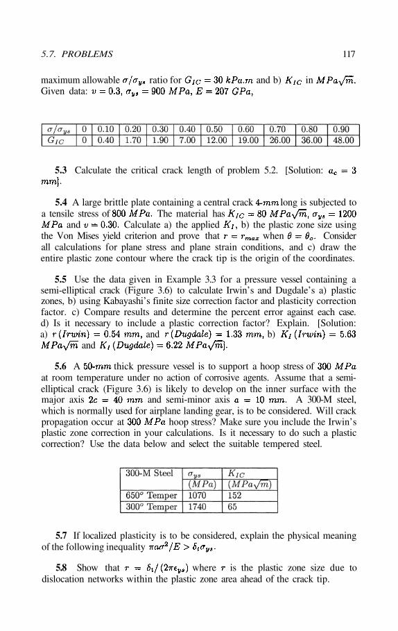
5.7. PROBLEMS 117
maximum allowable ratio for and b) inGiven data:
5.3 Calculate the critical crack length of problem 5.2. [Solution:
5.4 A large brittle plate containing a central crack long is subjected toa tensile stress of The material has
and Calculate a) the applied b) the plastic zone size usingthe Von Mises yield criterion and prove that when Considerall calculations for plane stress and plane strain conditions, and c) draw theentire plastic zone contour where the crack tip is the origin of the coordinates.
5.5 Use the data given in Example 3.3 for a pressure vessel containing asemi-elliptical crack (Figure 3.6) to calculate Irwin’s and Dugdale’s a) plasticzones, b) using Kabayashi’s finite size correction factor and plasticity correctionfactor. c) Compare results and determine the percent error against each case.d) Is it necessary to include a plastic correction factor? Explain. [Solution:a) and b)
and
5.6 A thick pressure vessel is to support a hoop stress ofat room temperature under no action of corrosive agents. Assume that a semi-elliptical crack (Figure 3.6) is likely to develop on the inner surface with themajor axis and semi-minor axis A 300-M steel,which is normally used for airplane landing gear, is to be considered. Will crackpropagation occur at hoop stress? Make sure you include the Irwin’splastic zone correction in your calculations. Is it necessary to do such a plasticcorrection? Use the data below and select the suitable tempered steel.
5.7 If localized plasticity is to be considered, explain the physical meaningof the following inequality
5.8 Show that where is the plastic zone size due todislocation networks within the plastic zone area ahead of the crack tip.
5.17 Show that for plane stress conditions. Schemat-ically, plot for various a and fixed a values.
118 CHAPTER 5. CRACK TIP PLASTICITY
5.9 Show that and give a reasonable interpretation ofthis equality.
5.10 A large strong plate containing a through-the-thickness central crackof has and atservice temperature. Determine a) the plane strain fracture toughness, b) thedesign stress intensity factor for a safety factor of 2, c) the critical fracturestress, and d) the design service stress.
5.11 Predict for a glass using
5.12 Derive an expression for using a Von Mises material. Compare itwith that for a Tresca material under plane strain conditions.
5.13 A material has and hasto be used as a plate in a large structure. Non-destructive evaluation detectsa central crack of long. If the displacement at fracture isand the plate width is three times the thickness, calculate a) the crack tipopening displacement, b) the plane strain fracture toughness, c) the plane strain-energy release rate, d) the plate thickness and e) What’s the safety factor beingindirectly included in this elastic-plastic fracture mechanics approach? Assumeplane strain conditions as per eq. (5.31) and a fracture load of [Solution:a) b) c) d)
and e)
5.14 Repeat problem 5.13 using eq. (5.41). Compare results.
5.15 A hypothetical large metallic plate containing a central crack iswide and thick and mechanically loaded in tension. This plate has
and for plane stress strain.Determine a) b) and c) as per Irwin, Dugdale, Burdekin and Riceequations. Compare results. {Solution: a) b)and c)
5.16 Determine a) the critical crack tip opening displacement b) theplastic zone size and c) the fracture stress for a large aluminum alloyplate containing a central crack of long. Use the following available dataand assume plane strain conditions: and
It
[1] W.W. Dally and W.F. Riley, “Experimental Stress Analysis,” Third Edition,McGraw-Hill, Inc. New York, (1991)
[2] G.R. Irwin, “Fracture I,” in S. Flugge (ed.), Handbuch der Physik VI,Springer-Verlag, New York, (1958)
[3] S.P. Timoshenko and J.N. Goodier, “Theory of Elasticity,” third edition,McGraw-Hill Co., New York, (1970) 142
[4] J.R. Rice, Proc. 1st Inter. Conf. On Fracture, Sendai, 1965, Editedby T. Yokobori, et al., Japanese Society for strength and Fracture of Materials,Tokyo, Vol. I, (1966) 283
[5] H.M. Westergaard, “Bearing Pressures and Cracks,” J. Appl. Mech.,G1 (1939) A49 - A53
[6] D. Broek, “Elementary Engineering Fracture Mechanics,” Fourth edi-tion, Kluwer Academic Publisher, Boston, (1986)
[7] K. Hellan, “Introduction to Fracture Mechanics,” McGraw-Hill Bookcompany, New York, (1984)
[8] R.W. Hertzberg, “Deformation and Fracture Mechanics of EngineeringMaterials,” Third edition, John Wiley & Sons, New York, (1989)
[9] G.R. Irwin, Proc. SESA, Vol. XVI, No. 1 (1958) 93-96[10] M.H. Aliabadi and D.P. Rooke, ”Numerical Fracture Mechanics,” Com-
putational Mechanics Publications, Kluwer Academic Publishers, Boston, (1992)Chapter 2.
[11] J.D. Eshelby, Proc. Roy. Soc., Series A 241, (1957) 376[12] A.N. Stroh, Adv. Physics, 6(1957) 418.[13] K.E. Puttick, Phil. Mag., 4 (1959) 964.[14] H.C. Rogers, Trans. Met. Soc. AIME, 218 (1960) 498[15] J. Gurland and J. Plateau, ASM Trans. Quart., 56 (1963) 442[16] R. Chona, “Non-singular Stress Effects in Fracture Test Specimens - A
Photoelastic Study,” M.S. Thesis, University of Maryland, College Park, (Au-gust 1985)
[17] R.J. Sanford, “A critical Re - Examination of the Westergaard Methodfor Solving Opening Mode Crack Problems,” Mech. Res., Vol. 6, No. 5, (1979)289-294
[18] M.L. Williams, J. Appl. Mech., 24 (1957) 109 - 114[19] H.O. Fuchs and R.I. Stephens, “Metal Fatigue in Engineering,” John
Wiley & Sons, New York, 1980[20] J.A. Collins, “Failure of Materials in Mechanical Design: Analysis, Pre-
diction, Prevention,” John Wiley & Sons, New York, (1981)[21] G.R. Irwin, “Plastic Zone near a Crack and Fracture Toughness,” Proc.
7th Sagamore conference, (1960) IV-63[22] J.R. Low, Progr. Mater. Sci., 12 (1) (1963)[23] J.R. Rice, in “Fracture an Advanced Treatise,” edited by H. Liebowitz,
Academic Press, New York, Vol. II, (1968) 191[24] D.S. Dugdale, “Yielding of Steel Sheets Containing Slits,” J. Mech.
Phys. Sol. 8(1960) 100-108
5.8. REFERENCES 119
5.8 REFERENCES
[25] F.A. McClintock and G.R. Irwin, “Plasticity Aspects of Fracture Me-chanics,” ASTM STP 381, (1965) 84-113
[26] I.S. Tuba, “A method of Elastic-Plastic Plane Stress and Plane StrainAnalysis,” J. Strain Analysis, 1 (1966) 115-122
[27] J.H. Underwood and D.P. Kendall, “Measurement of Plastic Strain Dis-tribution in the Region of a Crack Tip,” Exp. Mechanics (1969) 296-304
[28] G.T. Hahn and A.R. Rosenfield, “Plastic Flow in the Locale on Notchesand Cracks in Fe-3Si Steel under Condition Approaching Plane Strain,” Reportto ship structure committee (1968)
[29] J.R. Rice and G.F. Rosengren, “Plane Strain Deformation near a CrackTip in a Power-Law Hardening Material”, J. Mech. Phys. Sol., 16 (1968) 1
[30] B.A. Bilby and K.H. Swiden, “Representation of Plasticity at Notchesby Linear Dislocation Arrays”, Proc. Royal Soc. A285 (19650 22-30
[31] G.T. Hahn and A.R. Rosenfield, “Local Yielding and Extension of aCrack Under Plane Stress,” Acta Metallurgica, 13 (March 1965) 293-306
[32] D. Broek, “A Study on Ductile Fracture,” Nat. Aerospace Inst. Ams-terdam, Report TR 71021 (1971)
[33] V.Z. Parton and E.M. Morozov, “Mechanics of Elastic-Plastic Fracture,”second edition, Hemisphere publishing corporation, New York, (1989)
[34] P.S. Theocaris and N.P. Andrianopoulos, “The Mises Elastic-PlasticBoundary as the Core Region in Fracture Criteria,” Engineering Fracture Me-chanics, 16 (3) (1982) 425-432
[35] ASTYME1290, standard method for crack-tip opening Displacement(CTOD) Fracture Toughens Measurement, (1998) 846
[36] A.R. Rosenfield, et al., Proc. 1st International Conference on Fracture,Sendai, Edited by T. Yokobori, et al. (1965) 223
[37] T.H. Courtney, “Mechanical Behavior of Materials,” McGraw-Hill Co.,New York, (1990)
[38] A.A. wells, British Welding Research Association Rep., M13 (1963)[39] F.M. Burdekin, and D.E. Stone, J. Strain Analysis, 1 (1966) 145[40] D. Broek and h. Vlieger, National Aerospace Lab. TR 74032, (1974)[41] J.N. Robinson and A.S. Tetelman, Un. Cal. Los Angeles Report Eng.
7360 (1973)[42] C.Q. Bowles, Army Mat. And Mech. Research Center, Watertown,
Massachusetts,Report AMMRC Cr 70-23, (1970)[43] J.F. Lancaster, “Metallurgy of Welding,” Fifth ed., Chapman & Hall,
New York, (1993)[44] M.A. Meyers and K.K. Chawla, “Mechanical Behavior of Materials,”
Prentice Hall, Upper Saddle River, New Jersey, (1999) 358
120 CHAPTER 5. CRACK TIP PLASTICITY
Chapter 6
THE ENERGYPRINCIPLE
6.1
In this chapter, the elastic behavior of solids containing cracks is examined usingthe energy principal approach, which includes all forms of energy since loadingdevelops mechanical work, energy absorption around the crack tip, and energydissipation as heat. Williams [1] and Broek [2] undertook this energy approachas the primary form of energy (mechanical work ) being considered. If work isdone, then crack growth occurs and elastic energy is released. With the excep-tion of pure brittle solids, engineering materials undergo some form of plasticdeformation at the crack tip due to an applied external stress. Such plasticdeformation is an irreversible process and the material undergoes a plastic flowprocess.
In a general sense, plastic flow is referred to as a permanent and non-recoverable deformation in most common solid materials. On the other hand,viscous flow describes the mechanical behavior of plastics, such as non-crystallinepolymers, and it is temperature and time dependent. The term viscoelasticityis also used to indicate viscous flow.
6.2 ENERGY RELEASE RATE
The focus of this section is to determine the energy balance and the crack drivingforce for a slow crack growth event due to the action of an external quasi-staticload. The crack may be embedded, on the surface or through-the-thickness.Consider a body with a boundary contour as shown in Figure 6.1 subjectedto an energy input increment due to an external loading [1,7]. Assume thatthe solid body is elastic and its elastic mechanical behavior can be characterizedby a linear load-displacement relationship, as depicted in Figure 6.2
INTRODUCTION
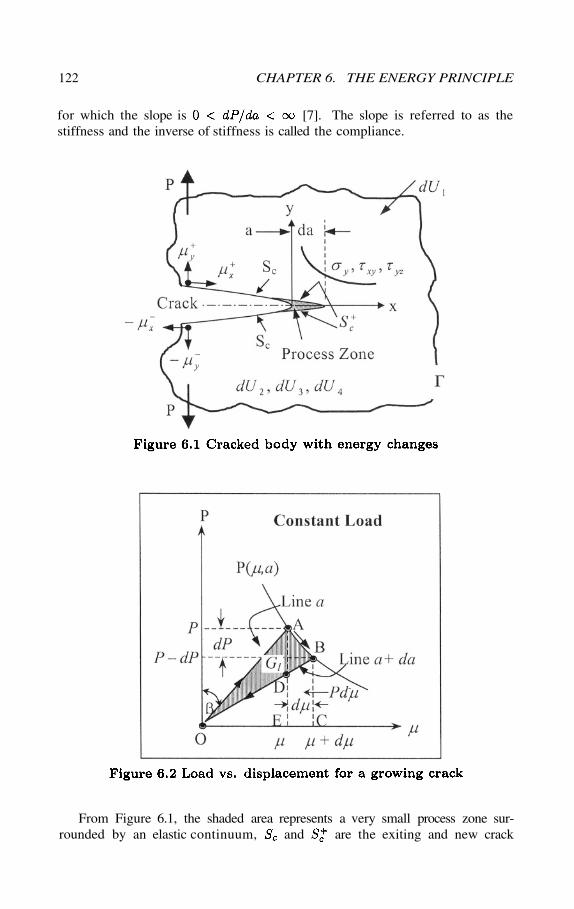
122 CHAPTER 6. THE ENERGY PRINCIPLE
for which the slope is [7]. The slope is referred to as thestiffness and the inverse of stiffness is called the compliance.
From Figure 6.1, the shaded area represents a very small process zone sur-rounded by an elastic continuum, and are the exiting and new crack
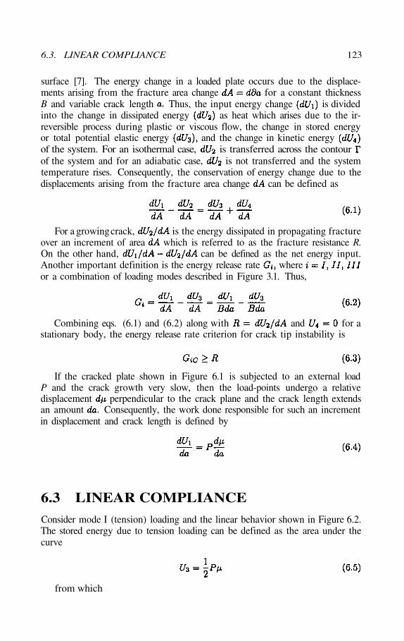
6.3. LINEAR COMPLIANCE 123
surface [7]. The energy change in a loaded plate occurs due to the displace-ments arising from the fracture area change for a constant thicknessB and variable crack length Thus, the input energy change is dividedinto the change in dissipated energy as heat which arises due to the ir-reversible process during plastic or viscous flow, the change in stored energyor total potential elastic energy and the change in kinetic energyof the system. For an isothermal case, is transferred across the contourof the system and for an adiabatic case, is not transferred and the systemtemperature rises. Consequently, the conservation of energy change due to thedisplacements arising from the fracture area change can be defined as
6.3 LINEAR COMPLIANCE
Consider mode I (tension) loading and the linear behavior shown in Figure 6.2.The stored energy due to tension loading can be defined as the area under thecurve
from which
For a growing crack, is the energy dissipated in propagating fractureover an increment of area which is referred to as the fracture resistance R.On the other hand, can be defined as the net energy input.Another important definition is the energy release rate whereor a combination of loading modes described in Figure 3.1. Thus,
Combining eqs. (6.1) and (6.2) along with and for astationary body, the energy release rate criterion for crack tip instability is
If the cracked plate shown in Figure 6.1 is subjected to an external loadP and the crack growth very slow, then the load-points undergo a relativedisplacement perpendicular to the crack plane and the crack length extendsan amount Consequently, the work done responsible for such an incrementin displacement and crack length is defined by
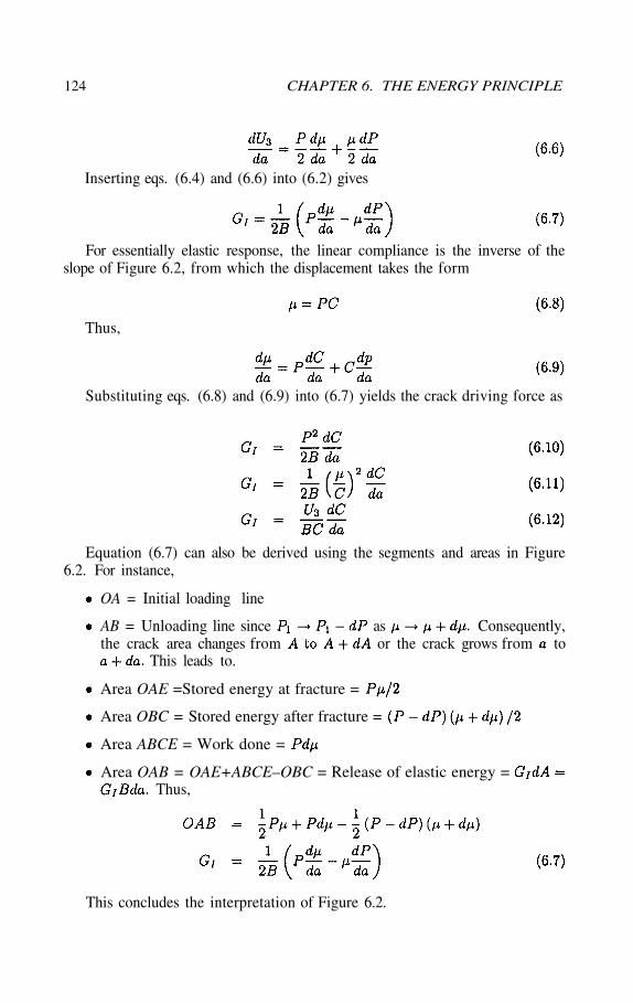
124 CHAPTER 6. THE ENERGY PRINCIPLE
Inserting eqs. (6.4) and (6.6) into (6.2) gives
For essentially elastic response, the linear compliance is the inverse of theslope of Figure 6.2, from which the displacement takes the form
Thus,
Substituting eqs. (6.8) and (6.9) into (6.7) yields the crack driving force as
Equation (6.7) can also be derived using the segments and areas in Figure6.2. For instance,
OA = Initial loading line
AB = Unloading line since as Consequently,the crack area changes from or the crack grows from to
This leads to.
Area OAE =Stored energy at fracture =
Area OBC = Stored energy after fracture =
Area ABCE = Work done =
Area OAB = OAE+ABCE–OBC = Release of elastic energy =Thus,
This concludes the interpretation of Figure 6.2.
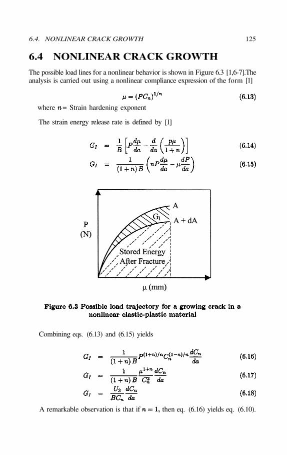
6.4. NONLINEAR CRACK GROWTH 125
6.4 NONLINEAR CRACK GROWTH
The possible load lines for a nonlinear behavior is shown in Figure 6.3 [1,6-7].Theanalysis is carried out using a nonlinear compliance expression of the form [1]
where = Strain hardening exponent
The strain energy release rate is defined by [1]
Combining eqs. (6.13) and (6.15) yields
A remarkable observation is that if then eq. (6.16) yields eq. (6.10).
126 CHAPTER 6. THE ENERGY PRINCIPLE
6.5 TRACTION FORCES
Consider two-dimensional problems in Cartesian system wherehas a unit length an it is treated here as a coordinate. Assume that the pathof the crack tip is along and that the origin is at the crack tip (Figure6.1) for a pure elastic state under quasi-static loading. This implies that thecrack area along with a unit length in the becomesBy definition, the traction excerpted through from the continuum on theprocess zone is where denotes the type of stress per stressing modeI, II or III.
According to Hellan [7], the magnitude of the traction forces on the upperand lower crack sides are and orrespectively. The corresponding displacements are and or
Moreover, the dominant stresses along the crack line can bedetermined at and the displacements along the crack sides atThis implies that the crack tip is located at for the principlestresses and for the displacements.
Accordingly, the translation of the fields at the crack front leads towhich is required to determine the limit of the crack driving force. This canclearly be appreciated by considering a two-dimensional analysis of a pure elasticsolid body subjected to a quasi-static loading as depicted in Figure 6.1. Thus,the strain energy release rate on the elastic continuum over the crack surface
can be defined by [7]
where = Differential surface area= Displacement increments at= Change in crack area= Representation of a stage for plastic process= Representation of a stage for crack extension
In order to solve eq. (6.21), the stresses and the displacements for the threemodes of loading (as depicted in Figure 3.1) being derived in Chapter 4 can bedefined in a general form by replacing the plastic zone size for in the stressequations for each stress mode and for in the displacement equationswhen crack extension occurs.
6.5. TRACTION FORCES 127
For the symmetric mode I at and
For the antisymmetric mode II at and
For the antisymmetric mode III at
From Chapter 4, the constant is defined by
Substituting eqs. (6.24), (6.27) and (6.30) into (6.21) yields the crack drivingforce for a mixed-mode interaction
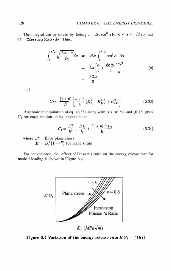
128 CHAPTER 6. THE ENERGY PRINCIPLE
The integral can be solved by letting for so thatThus,
and
Algebraic manipulation of eq. (6.33) along with eqs. (6.31) and (6.32) givesfor crack motion on its tangent plane
where for plane stressfor plane strain
For convenience, the effect of Poisson’s ratio on the energy release rate formode I loading is shown in Figure 6.4.
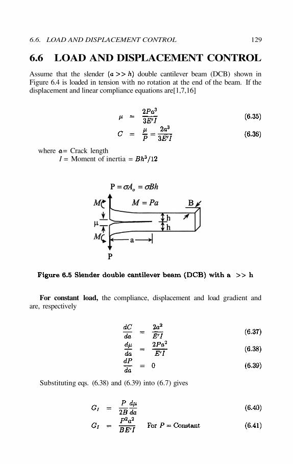
6.6. LOAD AND DISPLACEMENT CONTROL 129
6.6 LOAD AND DISPLACEMENT CONTROL
Assume that the slender double cantilever beam (DCB) shown inFigure 6.4 is loaded in tension with no rotation at the end of the beam. If thedisplacement and linear compliance equations are[1,7,16]
where = Crack lengthI = Moment of inertia =
For constant load, the compliance, displacement and load gradient andare, respectively
Substituting eqs. (6.38) and (6.39) into (6.7) gives
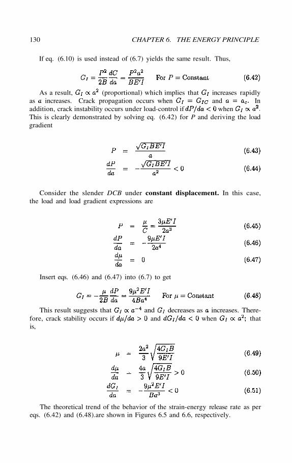
130 CHAPTER 6. THE ENERGY PRINCIPLE
If eq. (6.10) is used instead of (6.7) yields the same result. Thus,
As a result, (proportional) which implies that increases rapidlyas increases. Crack propagation occurs when and Inaddition, crack instability occurs under load-control if whenThis is clearly demonstrated by solving eq. (6.42) for P and deriving the loadgradient
Consider the slender DCB under constant displacement. In this case,the load and load gradient expressions are
Insert eqs. (6.46) and (6.47) into (6.7) to get
This result suggests that and decreases as increases. There-fore, crack stability occurs if and when thatis,
The theoretical trend of the behavior of the strain-energy release rate as pereqs. (6.42) and (6.48).are shown in Figures 6.5 and 6.6, respectively.
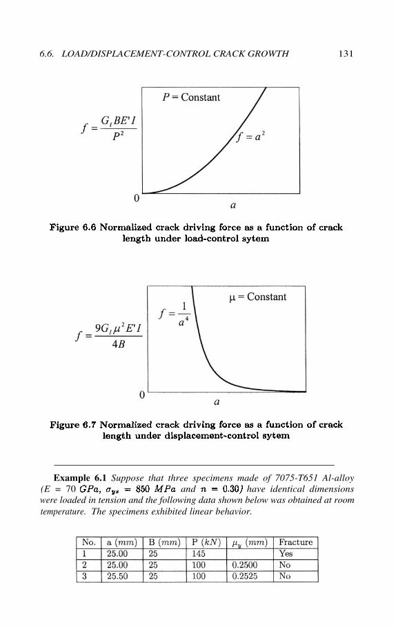
6.6. LOAD/DISPLACEMENT-CONTROL CRACK GROWTH 131
Example 6.1 Suppose that three specimens made of 7075-T651 Al-alloy(E = 70 and have identical dimensionswere loaded in tension and the following data shown below was obtained at roomtemperature. The specimens exhibited linear behavior.
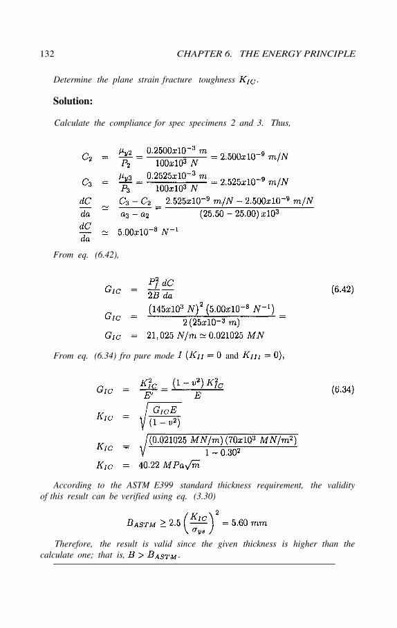
132 CHAPTER 6. THE ENERGY PRINCIPLE
Determine the plane strain fracture toughness
Solution:
Calculate the compliance for spec specimens 2 and 3. Thus,
From eq. (6.42),
From eq. (6.34) fro pure mode and
According to the ASTM E399 standard thickness requirement, the validityof this result can be verified using eq. (3.30)
Therefore, the result is valid since the given thickness is higher than thecalculate one; that is,
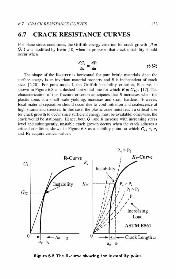
6.7. CRACK RESISTANCE CURVES 133
6.7 CRACK RESISTANCE CURVES
For plane stress conditions, the Griffith energy criterion for crack growthwas modified by Irwin [10] when he proposed that crack instability should
occur when
The shape of the R-curve is horizontal for pure brittle materials since thesurface energy is an invariant material property and R is independent of cracksize. [2,20]. For pure mode I, the Griffith instability criterion, R-curve, isshown in Figure 6.8 as a dashed horizontal line for which [17]. Thecharacterization of this fracture criterion anticipates that R increases when theplastic zone, at a small-scale yielding, increases and strain hardens. However,local material separation should occur due to void initiation and coalescence athigh strains and stresses. In this case, the plastic zone must reach a critical sizefor crack growth to occur since sufficient energy must be available; otherwise, thecrack would be stationary. Hence, both and R increase with increasing stresslevel and subsequently, unstable crack growth occurs when the crack adheres acritical condition, shown in Figure 6.8 as a stability point, at whichand acquire critical values.
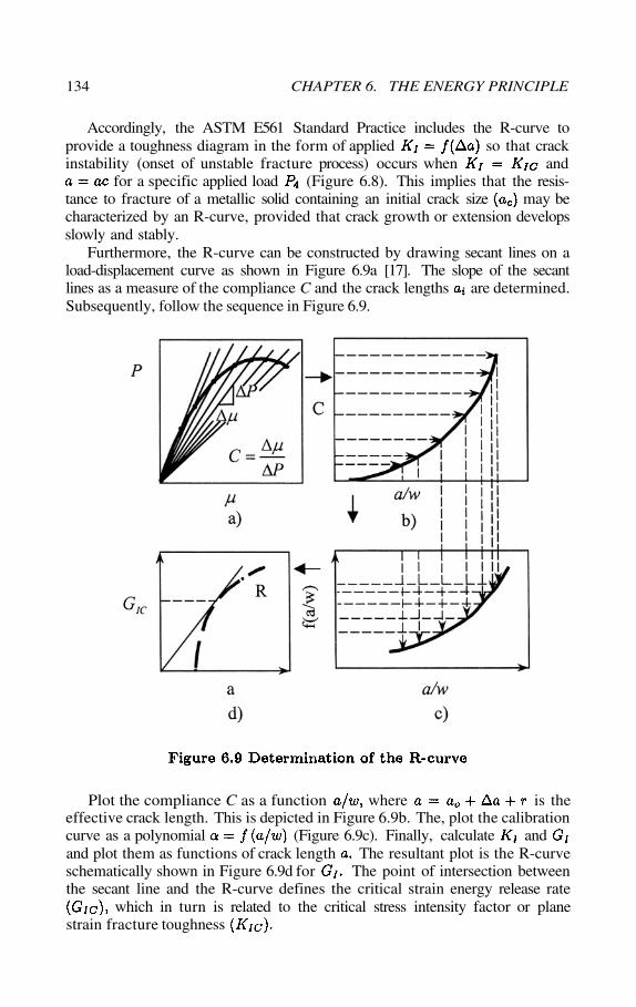
134 CHAPTER 6. THE ENERGY PRINCIPLE
Accordingly, the ASTM E561 Standard Practice includes the R-curve toprovide a toughness diagram in the form of applied so that crackinstability (onset of unstable fracture process) occurs when and
for a specific applied load (Figure 6.8). This implies that the resis-tance to fracture of a metallic solid containing an initial crack size may becharacterized by an R-curve, provided that crack growth or extension developsslowly and stably.
Furthermore, the R-curve can be constructed by drawing secant lines on aload-displacement curve as shown in Figure 6.9a [17]. The slope of the secantlines as a measure of the compliance C and the crack lengths are determined.Subsequently, follow the sequence in Figure 6.9.
Plot the compliance C as a function where is theeffective crack length. This is depicted in Figure 6.9b. The, plot the calibrationcurve as a polynomial (Figure 6.9c). Finally, calculate andand plot them as functions of crack length The resultant plot is the R-curveschematically shown in Figure 6.9d for The point of intersection betweenthe secant line and the R-curve defines the critical strain energy release rate
which in turn is related to the critical stress intensity factor or planestrain fracture toughness
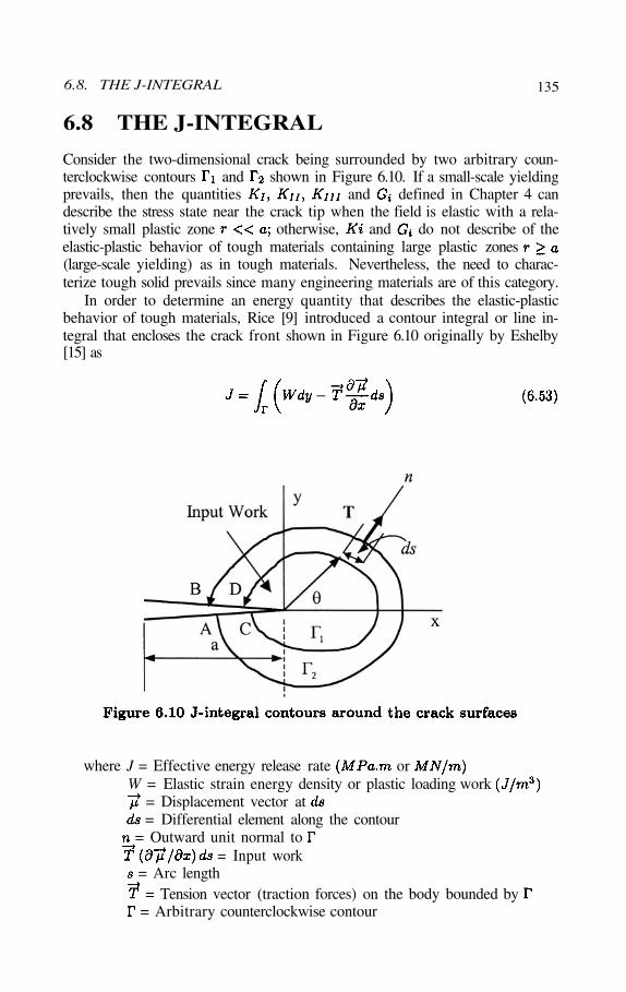
6.8. THE J-INTEGRAL 135
6.8 THE J-INTEGRAL
Consider the two-dimensional crack being surrounded by two arbitrary coun-terclockwise contours and shown in Figure 6.10. If a small-scale yieldingprevails, then the quantities and defined in Chapter 4 candescribe the stress state near the crack tip when the field is elastic with a rela-tively small plastic zone otherwise, and do not describe of theelastic-plastic behavior of tough materials containing large plastic zones(large-scale yielding) as in tough materials. Nevertheless, the need to charac-terize tough solid prevails since many engineering materials are of this category.
In order to determine an energy quantity that describes the elastic-plasticbehavior of tough materials, Rice [9] introduced a contour integral or line in-tegral that encloses the crack front shown in Figure 6.10 originally by Eshelby[15] as
where J = Effective energy release rateW = Elastic strain energy density or plastic loading work
= Displacement vector at= Differential element along the contour
= Outward unit normal to= Input work
= Arc length= Tension vector (traction forces) on the body bounded by
= Arbitrary counterclockwise contour
or
136 CHAPTER 6. THE ENERGY PRINCIPLE
The term J in eq. (6.53) is a line of surface integral defined around a contourIt characterizes the stress-strain field around the crack front and therefore, it
must be the energy release to the crack tip during crack growth. Due to thisfact, the J-integral is used as failure criterion and it is a measure of the fracturetoughness at the onset of slow crack growth for elastic and elastic-plastic metallicmaterials. The inherent characteristics of the J-integral exhibits a) remarkablepath, contour size and shape independence, and b) an invariability in magnitudewhen the contour lies either inside or outside the plastic zone [18]. The formercharacteristic indicates that the J-integral vanishes (J = 0) around an arbitraryclosed contour as shown by Parton and Morozov [19] using Green’s formula.
The interpretation of the J-integral includes the following observations:
The J-integral vanishes along the closed contours and because thetraction forces along the crack lower and upper surfaces are zeroand along AC and BD. Thus, eq. (6.53) becomesTherefore, the J-integral is path independent and it is a measure of thestraining at the crack tip that accounts for significant plastic deformationat the onset of crack initiation. The contour path can be defined arbitrarilyfor computational advantages [7], as it will be shown in a later section,since J is conserved. This means that the contour can conveniently bedefined along the plastic zone boundary so that the Von Mises plastic zonesize, eq. (3.52), can define the contour shape as shown in Figure 5.6.
The crack line can be included in the contour or without contributingto the value of J. For this reason, points A and B or C and D do notneed to coincide.
The J-integral along a contour around the crack is the change in potentialenergy (elastic energy) for a virtual crack extension Thus, the J-integral can be defined by
Remarkably, the J-integral can be evaluated along remote paths, wheresmall crack-tip yielding does not interfere.
With regard to eq. (6.53), the work input and the strain energy density aredefined as
In general, the elastic stresses needed in eq. (6.56) are defined in matrixform
6.8. THE J-INTEGRAL 137
The train energy density can be expressed as
Recall that plane stress condition requires that andConsequently, eq. (6.58) reduces to
For pure tension loading, W becomes
However, the elastic mixed-mode interaction described by eq. (6.34) can beused to predict the J-integral, provided that This means thatso that
6.8.1 FRACTURE CRITERION
The J-integral is used as a critical parameter for determining the onset of stablecrack growth and predicting fracture toughness. The fracture criterion byfor the initiation of stable crack growth is established when the applied J-integralreaches a critical value. This is indicated below for elastic and elastic-plasticmaterials
Similar fracture criteria can be used for mode II and III loading systems. Ingeneral, may be used as a brittle or ductile fracture toughness criterion forcharacterizing a material behavior that does not meet the requirements ofor fracture criterion. In addition, the measurement of is described bythe ASTM E399 Standard Testing Method, Vol. 03.01.
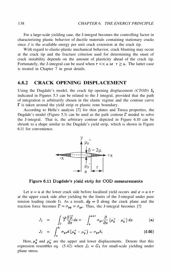
138 CHAPTER 6. THE ENERGY PRINCIPLE
For a large-scale yielding case, the J-integral becomes the controlling factor incharacterizing plastic behavior of ductile materials containing stationary crackssince J is the available energy per unit crack extension at the crack tip.
With regard to elastic-plastic mechanical behavior, crack blunting may occurat the crack tip and the fracture criterion used for determining the onset ofcrack instability depends on the amount of plasticity ahead of the crack tip.Fortunately, the J-integral can be used when The latter caseis treated in Chapter 7 in great details.
6.8.2 CRACK OPENING DISPLACEMENT
Using the Dugdale’s model, the crack tip opening displacement (CTOD)indicated in Figures 5.3 can be related to the J integral, provided that the pathof integration is arbitrarily chosen in the elastic regime and the contour curve
is taken around the yield strip or plastic zone boundary.According to Hella’s analysis [7] for thin plates and Tresca properties, the
Dugdale’s model (Figure 5.3) can be used as the path contour needed to solvethe J-integral. That is, the arbitrary contour depicted in Figure 6.10 can beshrunk to a shape similar to the Dugdale’s yield strip, which is shown in Figure6.11 for convenience.
Let at the lower crack side before localized yield occurs andat the upper crack side after yielding be the limits of the J-integral under puretension loading (mode I). As a result, along the crack plane and thetraction force becomes Thus, the J-integral becomes [7]
Here, and are the upper and lower displacements. Denote that thisexpression resembles eq. (5.42) when for small-scale yielding underplane stress.
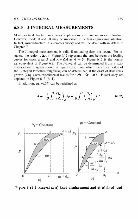
6.8. THE J-INTEGRAL 139
6.8.3 J-INTEGRAL MEASUREMENTS
Most practical fracture mechanics applications are base on mode I loading.However, mode II and III may be important in certain engineering situation.In fact, mixed-fracture in a complex theory and will be dealt with in details inChapter 7.
The J-integral measurement is valid if unloading does not occur. For in-stance, the region in Figure 6.12 represents the area between the loadingcurves for crack areas A and as Figure 6.12 is the nonlin-ear equivalent of Figure 6.2. The J-integral can be determined from a load-displacement diagram shown in Figure 6.12, from which the critical value ofthe J-integral (fracture toughness) can be determined at the onset of slow crackgrowth [7-8]. Some experimental results for a steel alloy aredepicted in Figure 6.13 [6,11].
In addition, eq. (6.54) can be redefined as
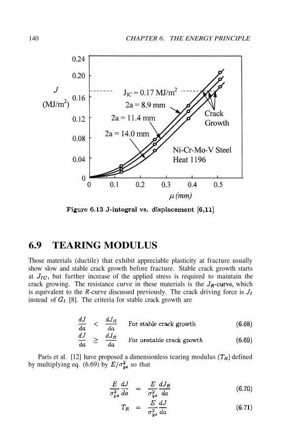
140 CHAPTER 6. THE ENERGY PRINCIPLE
6.9 TEARING MODULUS
Those materials (ductile) that exhibit appreciable plasticity at fracture usuallyshow slow and stable crack growth before fracture. Stable crack growth startsat but further increase of the applied stress is required to maintain thecrack growing. The resistance curve in these materials is the whichis equivalent to the R-curve discussed previously. The crack driving force isinstead of [8]. The criteria for stable crack growth are
Paris et al. [12] have proposed a dimensionless tearing modulus definedby multiplying eq. (6.69) by so that
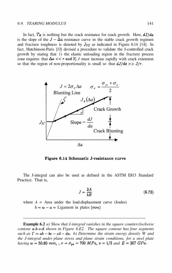
6.9. TEARING MODULUS 141
In fact, is nothing but the crack resistance for crack growth. Here,is the slope of the resistance curve in the stable crack growth regimenand fracture toughness is denoted by as indicated in Figure 6.14 [14]. Infact, Hutchinson-Paris [13] devised a procedure to validate the J-controlled crackgrowth by stating that 1) the elastic unloading region in the fracture processzone requires that J must increase rapidly with crack extensionso that the region of non-proportionality is small so that
The J-integral can also be used as defined in the ASTM E813 StandardPractice. That is,
where A = Area under the load-displacement curve (Joules)Ligament in plates
Example 6.2 a) Show that J-integral vanishes in the square counterclockwisecontour shown in Figure 6.E2. The square contour has four segmentssuch as b) Determine the strain energy density W andthe J-integral under plane stress and plane strain conditions, for a steel platehaving and
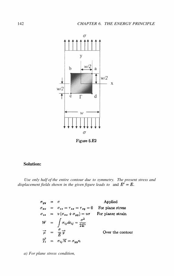
142 CHAPTER 6. THE ENERGY PRINCIPLE
Solution:
Use only half of the entire contour due to symmetry. The present stress anddisplacement fields shown in the given figure leads to and
a) For plane stress condition,
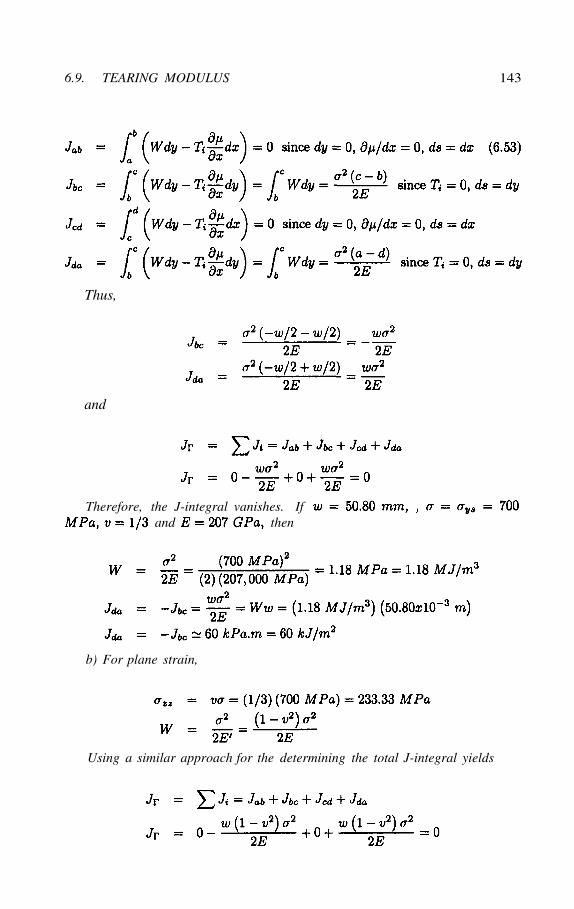
6.9. TEARING MODULUS 143
and
Therefore, the J-integral vanishes. Ifand then
b) For plane strain,
Using a similar approach for the determining the total J-integral yields
Thus,
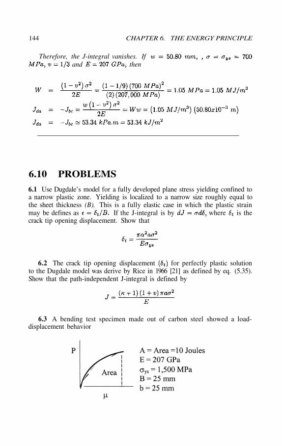
144 CHAPTER 6. THE ENERGY PRINCIPLE
Therefore, the J-integral vanishes. Ifand then
6.10 PROBLEMS
6.1 Use Dugdale’s model for a fully developed plane stress yielding confined toa narrow plastic zone. Yielding is localized to a narrow size roughly equal tothe sheet thickness (B). This is a fully elastic case in which the plastic strainmay be defines as If the J-integral is by where is thecrack tip opening displacement. Show that
6.2 The crack tip opening displacement for perfectly plastic solutionto the Dugdale model was derive by Rice in 1966 [21] as defined by eq. (5.35).Show that the path-independent J-integral is defined by
6.3 A bending test specimen made out of carbon steel showed a load-displacement behavior
6.11. REFERENCES 145
If the area under the curve the is 10 joules at the onset of crackgrowth, determine a) the fracture toughness in terms of as per ASTM E813Standard, b) and its validity as per ASTM E399 testing method, and c)using eq. (5.31) with d) the fracture strain, e) the displacement and f)the plastic zone size. Explain the meaning of the results. [Solution: a)
b) c) d) e)and f)
6.4 If is used to determine the fracture toughness, will be apath-independent entity? Explain.
6.5 Assume hat crack growth occurs when If a well-developedplastic flow occurs, will this inequality be valid? Explain.
6.11 REFERENCES[1] J.G. Williams,“Fracture Mechanics of Polymers,” Ellis Horwood Limited,Halsted Press: a Division of John Wiley & Sons, New York, (1984).
[2] D. Broek, “Elementary Engineering Fracture Mechanics,” Fourth edi-tion, Kluwer Academic Publisher, Boston, (1986).
[3] C.E. Inglis, “Stresses in a Plate due to the Presence of Cracks and SharpCorners,” Trans. Inst. Nav. Arch., 55 (1913) 219-241.
[4] A.A. Griffith, Phil. Trans. Royal Soc., 221 (1921) 163-167[5] H.M. Westergaard, “Bearing Pressures and Cracks,” J. Appl. Mech.,
G1 (1939) A49-A53[6] D. Broek, “Elementary Engineering Fracture Mechanics,” Fourth edi-
tion, Kluwer Academic Publisher, Boston, (1986)[7] K. Hellan, “Introduction to Fracture Mechanics”, McGraw-Hill Book,
New York, (1984)[8] R.W. Hertzberg, “Deformation and Fracture Mechanics of Engineering
Materials,” third edition, John Wiley & Sons, New York, (1989)[9] J.R. Rice, J. Appl. Mech. 35 (1968) 379-386[10] G.R. Irwin, ASTM Bulletin, (Jan. 1960) 29[11] J.D. Landes and J.A. Begley, ASTM STP 514, (1972) 24-39[12] P. C. Paris, H. Tada, A. Zahoor and H. Ernst, “Instability of the Tearing
Model of Elastic-Plastic Crack Growth,” ASTM STP 668, (1979) 5.36.[13] J.E.W. Hutchinson and P.C. Paris, in Elastic -Plastic Fracture, ASTM
STP 668, (1979) 37.[14] S. Surch and A.K. Vasudevan, “On the Relationship between Crack
Initiation Toughness and Crack Growth,” Math. Sci. Eng., “79 (1986) 183-190.[15] J.D. Eshelby, “Calculation of Energy Release Rate,” in Prospects of
Fracture Mechanics, G.C. Sih, H.C. Von Elst, and D. Broek, Noordhoff, Growin-gen, (1974) 69-84.

146 CHAPTER 6. THE ENERGY PRINCIPLE
[16] D.K. Felbeck and A.G. Atkins, “Strength and Fracture of EngineeringSolids,” Second Edition, Prentice-Hall, Inc., Upper Saddle River, N.J. (1996)430-443
[17] ASTM 351-94, Annual Book of ASTM Standards, Vol. 03.01[18] E.M. Morozov and G.P. Nikishkov, “Finite Element Method in Fracture
Mechanics,” Nauka, Moscow, (1980), reference cited in [19].[19] V.Z. Parton and E.M. Morozov, “Mechanics of Elastic-Plastic Fracture,”
second edition, Hemisphere publishing corporation, New York, (1989)[20] T.L. Anderson, “Fracture Mechanics: Fundamentals and Applications,”
CRC Press, Inc., Boston, (1991) 58.
PLASTIC FRACTUREMECHANICS
This chapter describes the stress-strain fields at a crack tip for materials thatwill obey the Ramberg-Osgood nonlinear stress-strain relation. These materialsare considered to be strain hardenable , specially under tension loading. A two-dimensional field equations are characterized for ductile or low-strength mate-rials, which can be strain hardened at a large scale yielding. In fact, hardeningin a polycrystalline material is due to plastic deformation, in which disloca-tion motion is the primary phenomenon for this irreversible process. However,dislocation-imperfection interactions impede the mobility of dislocations leadingto strain hardening. For instance, the dislocation distribution within a plasticzone is normally a complex and mixed phenomenon.
The mechanism of fracture is related to plastic deformation at the crack tipwhere high stresses and strains are developed. Therefore, the use of a disloca-tion model for determining stresses and strains would be an ideal mathematicalapproach for predicting crack instability. Instead, for a cracked elastic-plasticmaterial subjected to an external load, the onset of plastic flow occurs at thecrack tip and the flow criterion that predicts the onset of crack instability is usu-ally the J-integral, which is limited to a stationary crack in a strain hardeningmaterial.
Hutchinson [1] and Rice and Rosengren [2] in separate publications in 1968showed that the J-integral characterizes the stress and strain fields at the cracktip in nonlinear elastic materials. Their work is referred to as the HRR the-ory, which is as an extension of linear fracture mechanics that account for a
Chapter 7
7.1 INTRODUCTION
7.2 J-CONTROLLED CRACK GROWTH
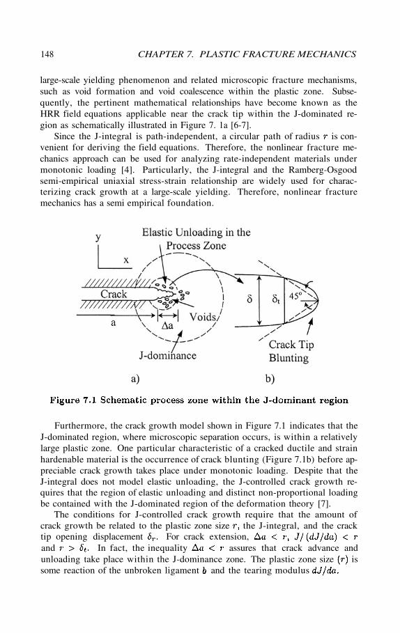
148 CHAPTER 7. PLASTIC FRACTURE MECHANICS
large-scale yielding phenomenon and related microscopic fracture mechanisms,such as void formation and void coalescence within the plastic zone. Subse-quently, the pertinent mathematical relationships have become known as theHRR field equations applicable near the crack tip within the J-dominated re-gion as schematically illustrated in Figure 7. 1a [6-7].
Since the J-integral is path-independent, a circular path of radius is con-venient for deriving the field equations. Therefore, the nonlinear fracture me-chanics approach can be used for analyzing rate-independent materials undermonotonic loading [4]. Particularly, the J-integral and the Ramberg-Osgoodsemi-empirical uniaxial stress-strain relationship are widely used for charac-terizing crack growth at a large-scale yielding. Therefore, nonlinear fracturemechanics has a semi empirical foundation.
Furthermore, the crack growth model shown in Figure 7.1 indicates that theJ-dominated region, where microscopic separation occurs, is within a relativelylarge plastic zone. One particular characteristic of a cracked ductile and strainhardenable material is the occurrence of crack blunting (Figure 7.1b) before ap-preciable crack growth takes place under monotonic loading. Despite that theJ-integral does not model elastic unloading, the J-controlled crack growth re-quires that the region of elastic unloading and distinct non-proportional loadingbe contained with the J-dominated region of the deformation theory [7].
The conditions for J-controlled crack growth require that the amount ofcrack growth be related to the plastic zone size the J-integral, and the cracktip opening displacement For crack extension,and In fact, the inequality assures that crack advance andunloading take place within the J-dominance zone. The plastic zone size issome reaction of the unbroken ligament and the tearing modulus
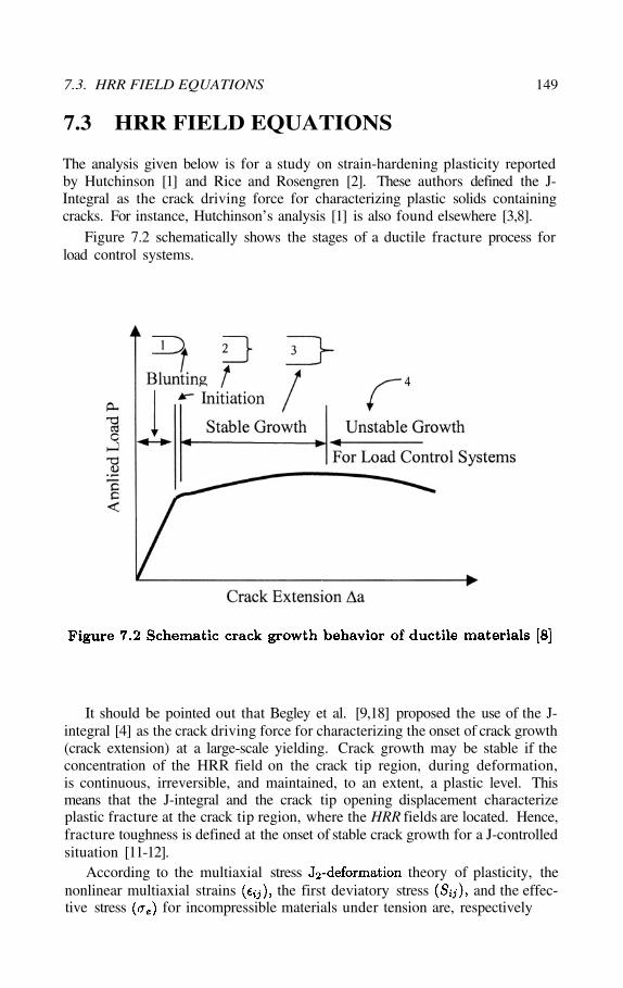
7.3. HRR FIELD EQUATIONS 149
The analysis given below is for a study on strain-hardening plasticity reportedby Hutchinson [1] and Rice and Rosengren [2]. These authors defined the J-Integral as the crack driving force for characterizing plastic solids containingcracks. For instance, Hutchinson’s analysis [1] is also found elsewhere [3,8].
Figure 7.2 schematically shows the stages of a ductile fracture process forload control systems.
It should be pointed out that Begley et al. [9,18] proposed the use of the J-integral [4] as the crack driving force for characterizing the onset of crack growth(crack extension) at a large-scale yielding. Crack growth may be stable if theconcentration of the HRR field on the crack tip region, during deformation,is continuous, irreversible, and maintained, to an extent, a plastic level. Thismeans that the J-integral and the crack tip opening displacement characterizeplastic fracture at the crack tip region, where the HRR fields are located. Hence,fracture toughness is defined at the onset of stable crack growth for a J-controlledsituation [11-12].
According to the multiaxial stress theory of plasticity, thenonlinear multiaxial strains the first deviatory stress and the effec-tive stress for incompressible materials under tension are, respectively
7.3 HRR FIELD EQUATIONS
In fact, the deformation theory of plasticity is basically a nonlinear elasticity[2]. The effective stress for plane stress is
and the effective stress and the strains for plane strain are [1]
With regard to the strain hardening exponent low-strength (ductile) ma-terials have greater hardening exponents than high-strength ones. As a result,large tensile stresses at the crack front in ductile materials cause nucleation ofvoids and void coalescence as the source for crack nucleation. Consequently,the effects of yielding and strain hardening at the crack front is a major con-cern in fracture mechanics. The phenomena of yielding and strain hardening isschematically shown in Figure 7.3 for quasi-static loading
150 CHAPTER 7. PLASTIC FRACTURE MECHANICS
where = Constant= Strain hardening exponent= Yield strain or reference strain= Yield strength or reference stress
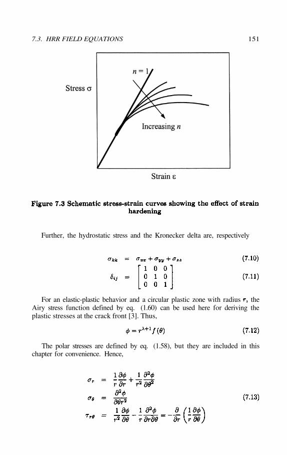
7.3. HRR FIELD EQUATIONS 151
Further, the hydrostatic stress and the Kronecker delta are, respectively
For an elastic-plastic behavior and a circular plastic zone with radius theAiry stress function defined by eq. (1.60) can be used here for deriving theplastic stresses at the crack front [3]. Thus,
The polar stresses are defined by eq. (1.58), but they are included in thischapter for convenience. Hence,
Inserting the partial derivatives of the Airy’s stress function, eq. (7.12), into(7.13) yields
One can observe that these stresses depend on The J-integral defined byeq. (6.53) along with eq. (4.6), and can bewritten as [2]
The remaining analytical procedure for deriving the trigonometric functionsfor the field equations is lengthy and complicated. Therefore, only relevantresults are included as reported in the literature. Important papers on thesubject are cited accordingly.
The essential mathematical approach for deriving the HRR field equationsis a well-developed method, and yet, a sophisticated technique for assessing theplastic J-integral [1-2]. Essentially, a rigorous computational skill is required toexplicitly characterize the crack behavior in the elastic-plastic regime, which isa complex nonlinearity manifested through the strain-hardening phenomenonat the crack tip region, where the J-controlled crack growth is characterized.
152 CHAPTER 7. PLASTIC FRACTURE MECHANICS
The boundary conditions can be set as
The strain compatibility equation that must be satisfied is of the form
Thus, the equivalent stress as defined by eq. (7.5) and (7.6), respectively,become
A ductile crack behavior, as opposed to brittle crack behavior, exhibits a sig-nificant crack tip blunting before the onset of crack growth (crack extension),complicating the applicability of the aforementioned mathematical technique[8]. Therefore, the resultant HRR field equations or HRR singularities nearthe crack tip for a stationary crack, as reported by Hutchinson [7] are
Mathematically, for a power-law hardening material, field equations at thecrack tip have singularities in the order shown below [2]
Figure 7.4 shows the numerical distribution of dimensionless stressand strain functions [1] and Table 7.1 gives
the numerical results for the constant Furthermore, the interpreta-tion of the strain-hardening exponent is based on the type of mechanicalbehavior of the solid material being tested and the size of the plastic zone interms of the crack length, such as for the J-controlled condition [23].For fully linear elasticity, the strain hardening is and the field equationshave a singularity in the order of andwhich is exactly the order as determined in Chapter 4. Conversely, forfully nonlinear plasticity so that
Furthermore, dividing eq. (7.21) by (7,20) yields the plastic zone size as
7.3. HRR FIELD EQUATIONS 153
where
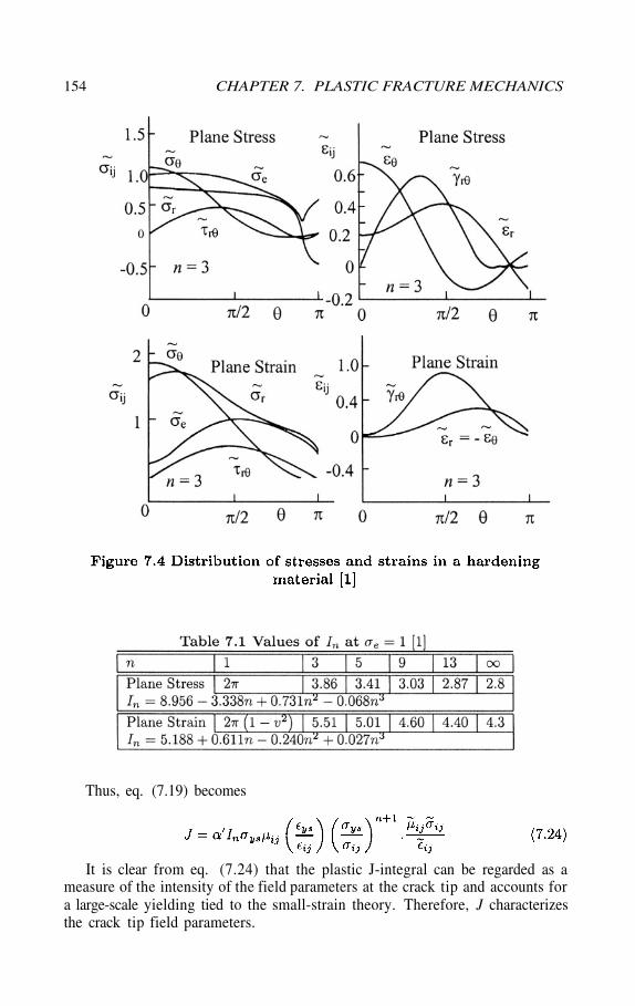
154 CHAPTER 7. PLASTIC FRACTURE MECHANICS
Thus, eq. (7.19) becomes
It is clear from eq. (7.24) that the plastic J-integral can be regarded as ameasure of the intensity of the field parameters at the crack tip and accounts fora large-scale yielding tied to the small-strain theory. Therefore, J characterizesthe crack tip field parameters.
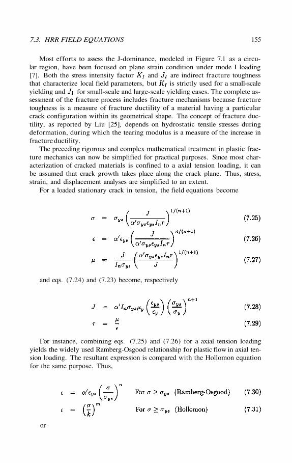
Most efforts to assess the J-dominance, modeled in Figure 7.1 as a circu-lar region, have been focused on plane strain condition under mode I loading[7]. Both the stress intensity factor and are indirect fracture toughnessthat characterize local field parameters, but is strictly used for a small-scaleyielding and for small-scale and large-scale yielding cases. The complete as-sessment of the fracture process includes fracture mechanisms because fracturetoughness is a measure of fracture ductility of a material having a particularcrack configuration within its geometrical shape. The concept of fracture duc-tility, as reported by Liu [25], depends on hydrostatic tensile stresses duringdeformation, during which the tearing modulus is a measure of the increase infracture ductility.
The preceding rigorous and complex mathematical treatment in plastic frac-ture mechanics can now be simplified for practical purposes. Since most char-acterization of cracked materials is confined to a axial tension loading, it canbe assumed that crack growth takes place along the crack plane. Thus, stress,strain, and displacement analyses are simplified to an extent.
For a loaded stationary crack in tension, the field equations become
For instance, combining eqs. (7.25) and (7.26) for a axial tension loadingyields the widely used Ramberg-Osgood relationship for plastic flow in axial ten-sion loading. The resultant expression is compared with the Hollomon equationfor the same purpose. Thus,
or
7.3. HRR FIELD EQUATIONS 155
and eqs. (7.24) and (7.23) become, respectively
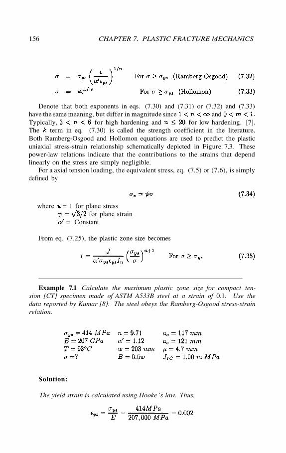
156 CHAPTER 7. PLASTIC FRACTURE MECHANICS
Denote that both exponents in eqs. (7.30) and (7.31) or (7.32) and (7.33)have the same meaning, but differ in magnitude since andTypically, for high hardening and for low hardening. [7].The term in eq. (7.30) is called the strength coefficient in the literature.Both Ramberg-Osgood and Hollomon equations are used to predict the plasticuniaxial stress-strain relationship schematically depicted in Figure 7.3. Thesepower-law relations indicate that the contributions to the strains that dependlinearly on the stress are simply negligible.
For a axial tension loading, the equivalent stress, eq. (7.5) or (7.6), is simplydefined by
From eq. (7.25), the plastic zone size becomes
Example 7.1 Calculate the maximum plastic zone size for compact ten-sion [CT] specimen made of ASTM A533B steel at a strain of 0.1. Use thedata reported by Kumar [8]. The steel obeys the Ramberg-Osgood stress-strainrelation.
where = 1 for plane stressfor plane strain
= Constant
Solution:
The yield strain is calculated using Hooke ’s law. Thus,
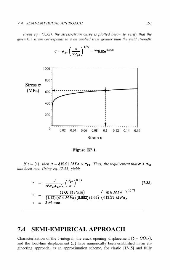
7.4. SEMI-EMPIRICAL APPROACH 157
From eq. (7.32), the stress-strain curve is plotted below to verify that thegiven 0.1 strain corresponds to a an applied tress greater than the yield strength.
If then Thus, the requirement thathas been met. Using eq. (7.35) yields
Characterization of the J-integral, the crack opening displacementand the load-line displacement have numerically been established in an en-gineering approach, as an approximation scheme, for elastic [13-15] and fully
7.4 SEMI-EMPIRICAL APPROACH
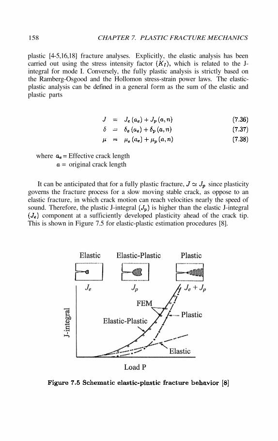
158 CHAPTER 7. PLASTIC FRACTURE MECHANICS
plastic [4-5,16,18] fracture analyses. Explicitly, the elastic analysis has beencarried out using the stress intensity factor which is related to the J-integral for mode I. Conversely, the fully plastic analysis is strictly based onthe Ramberg-Osgood and the Hollomon stress-strain power laws. The elastic-plastic analysis can be defined in a general form as the sum of the elastic andplastic parts
where = Effective crack length= original crack length
It can be anticipated that for a fully plastic fracture, since plasticitygoverns the fracture process for a slow moving stable crack, as oppose to anelastic fracture, in which crack motion can reach velocities nearly the speed ofsound. Therefore, the plastic J-integral is higher than the elastic J-integral
component at a sufficiently developed plasticity ahead of the crack tip.This is shown in Figure 7.5 for elastic-plastic estimation procedures [8].
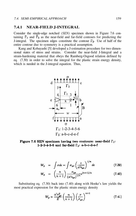
7.4. SEMI-EMPIRICAL APPROACH 159
Consider the single-edge notched (SEN) specimen shown in Figure 7.6 con-taining and as the near-field and far-field contours for predicting theJ-integral. The specimen edges constitute the contour Use of half of theentire contour due to symmetry is a practical assumption.
Kang and Kobayashi [5] developed a J-estimation procedure for two dimen-sional states of stress and strains. Consider the near-field J-Integral and astrain-hardening material that obeys the Ramberg-Osgood relation defined byeq. (7.30) in order to solve the integral for the plastic strain energy density,which is needed in the J-integral equation. Thus,
Substituting eq. (7.30) back into (7.40) along with Hooke’s law yields themost practical expression for the plastic strain energy density
7.4.1 NEAR-FIELD J-INTEGRAL
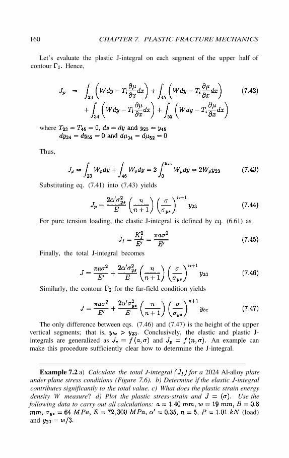
The only difference between eqs. (7.46) and (7.47) is the height of the uppervertical segments; that is, Conclusively, the elastic and plastic J-integrals are generalized as and An example canmake this procedure sufficiently clear how to determine the J-integral.
Example 7.2 a) Calculate the total J-integral for a 2024 Al-alloy plateunder plane stress conditions (Figure 7.6). b) Determine if the elastic J-integralcontributes significantly to the total value. c) What does the plastic strain energydensity W measure? d) Plot the plastic stress-strain and Use thefollowing data to carry out all calculations:
(load)and
160 CHAPTER 7. PLASTIC FRACTURE MECHANICS
Let’s evaluate the plastic J-integral on each segment of the upper half ofcontour Hence,
Thus,
Substituting eq. (7.41) into (7.43) yields
For pure tension loading, the elastic J-integral is defined by eq. (6.61) as
Finally, the total J-integral becomes
Similarly, the contour for the far-field condition yields
where
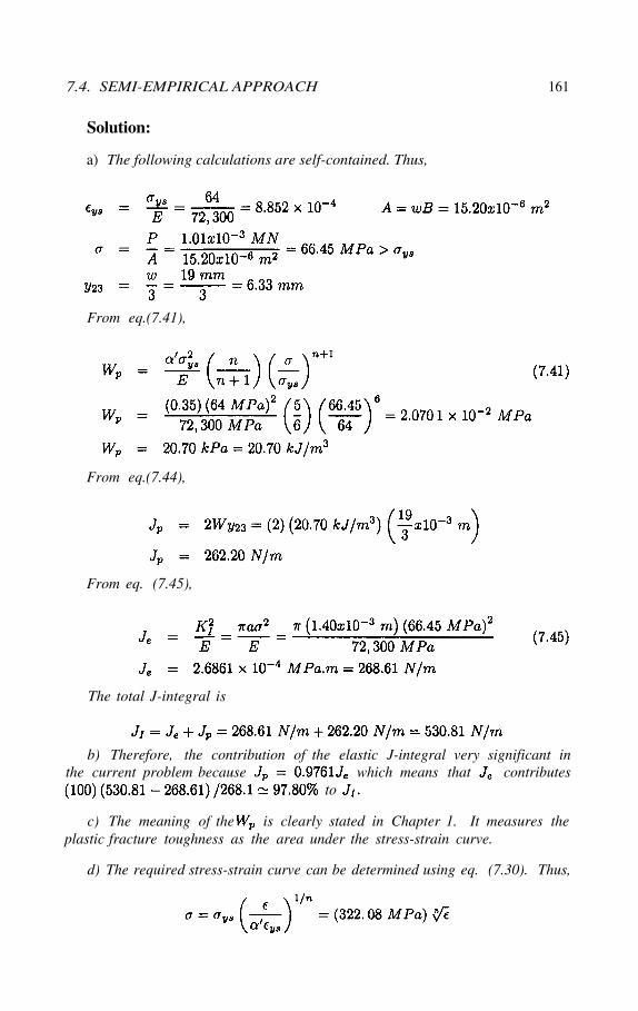
7.4. SEMI-EMPIRICAL APPROACH 161
Solution:
a) The following calculations are self-contained. Thus,
From eq.(7.41),
From eq.(7.44),
From eq. (7.45),
The total J-integral is
b) Therefore, the contribution of the elastic J-integral very significant inthe current problem because which means that contributes
to
c) The meaning of the is clearly stated in Chapter 1. It measures theplastic fracture toughness as the area under the stress-strain curve.
d) The required stress-strain curve can be determined using eq. (7.30). Thus,
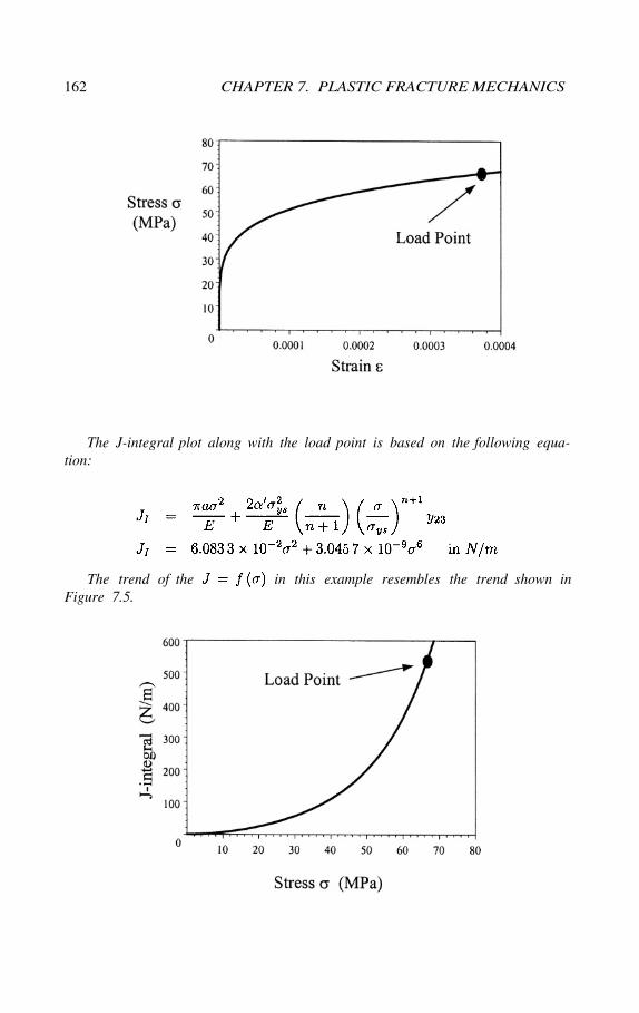
162 CHAPTER 7. PLASTIC FRACTURE MECHANICS
The J-integral plot along with the load point is based on the following equa-tion:
The trend of the in this example resembles the trend shown inFigure 7.5.
Consider the single-edge notched (SEN) specimen with contour as large as thespecimen shown in Figure 7.6 for characterizing the far-field J-integral using onlyhalf of the entire contour due to symmetry. The present stress field requires that
and for the assumed contour with segmentsand Thus, the far-field J-integral evaluation can be treated
as a reasonable approximation for the near-field. For an axial tension loading,Kang and Kobayashi [5] using Moiré interferometry evaluated the J-integral asthe sum of the vertical and horizontal parts of half the contour due to symmetry.Thus, the J-integral for the traction free vertical edges of the segments and
becomes
and that for the horizontal part along with and on thecrack line is
Kumar et al. [8] developed another approximation scheme for characterizingsimple specimen configurations. Assume that a material obeys the Ramberg-Osgood power law, eq. (7.30) and that the plastic field is controlled by theJ-integral for limited crack growth. It is also assumed that unloading doesnot occur behind the crack tip during the irreversible plastic deformation [11]and that the onset of unstable crack growth (crack propagation) occurs at themaximum load carrying capability of the component. The measurement of theJ-integral is carried out by determining the displacement from the deformationproperties of the Ramberg-Osgood material [21]
The simplified methodology for predicting fracture of structural componentsis based on eqs. (7.36) through (7.38) along with modified (7.30) and
7.5. ENGINEERING APPROACH 163
7.4.2 FAR-FIELD J-INTEGRAL
The total J-integral due to symmetry becomes
7.5 ENGINEERING APPROACH
and The general field equations for elastic-plastic fracture analysis aredefined as [8]
where P = Load per unit thickness
= Limit load per unit thickness
= Constant tabulated in Ref. [8]
= Constant tabulated in Ref. [13]
The constants and are defined in Table 7.2, and is Irwin’s effectivecrack length defined by
where = 2 for plane stress
= 6 for plane strain
The above field equations are strongly dependent on increasing load raisedto the power Therefore, the plastic part of these equations are dominant instrain hardenable and incompressible materials. Despite that these equationsrepresent approximations, they can provide satisfactorily accurate results of theJ-integral, strains and displacements in appropriate engineering applications.
164 CHAPTER 7. PLASTIC FRACTURE MECHANICS
with
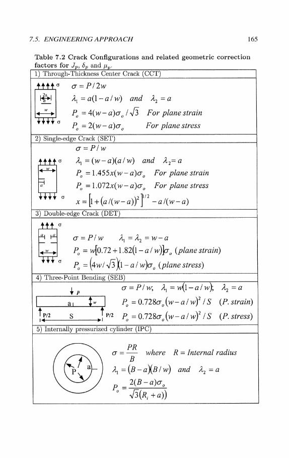
7.5. ENGINEERING APPROACH 165
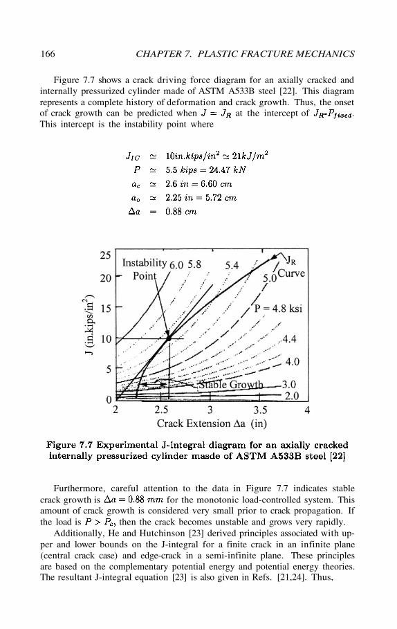
166 CHAPTER 7. PLASTIC FRACTURE MECHANICS
Figure 7.7 shows a crack driving force diagram for an axially cracked andinternally pressurized cylinder made of ASTM A533B steel [22]. This diagramrepresents a complete history of deformation and crack growth. Thus, the onsetof crack growth can be predicted when at the intercept ofThis intercept is the instability point where
Furthermore, careful attention to the data in Figure 7.7 indicates stablecrack growth is for the monotonic load-controlled system. Thisamount of crack growth is considered very small prior to crack propagation. Ifthe load is then the crack becomes unstable and grows very rapidly.
Additionally, He and Hutchinson [23] derived principles associated with up-per and lower bounds on the J-integral for a finite crack in an infinite plane(central crack case) and edge-crack in a semi-infinite plane. These principlesare based on the complementary potential energy and potential energy theories.The resultant J-integral equation [23] is also given in Refs. [21,24]. Thus,
7.5. ENGINEERING APPROACH 167
Let eq. (7.30) be an equivalent expression so that
Substituting eqs. (7.34) and (7.56) into (7.55) yields the upper bound J-integral for plane conditions
He and Hutchinson [23,24] also derived an upper bound form of the J-integralas defined below
where for a central crackfor an edge crack
Similarly, substitute eqs. (7.34) and (7.56) into (7.58) to get
It should be mention that both eqs. (7.57) and (7.59) should give similarresults. An example in the next section will prove this statement.
7.5.1 THE CONSTANT
The constant in eq. (7.51) can be derived for the specimen configurationsillustrated in Table 7.2. This can be done very easily by equating eqs. (7.51)and (7.57) and using the definitions of and The resultant expression are
For the central cracked plate given in Table 7.2,
where is defined in eq. (7.34).
Example 7.3 The application of the above procedure can be made clear byanalyzing the example given below. a) Calculate the total J-integral
for a center-crack plate made out of 2024 Al-alloy under plane conditions.Assume that the material obeys the Ramberg-Osgood relation. Use the followingdata:
and b) Plot for planestrain conditions. Explain.
Let’s determine using eq. (7.51) and Table 7.2
The calculated value of is close to the value tabulated by Kumar and Shih[8].
The other parameters are
168 CHAPTER 7. PLASTIC FRACTURE MECHANICS
Solution:
a) The solution requires the following parameters
From eq. (3.29) and Table 3.1, the applied stress intensity factor is
and from eq. (6.61) for pure tension loading, the elastic J-integral becomes
The constant along with and is
7.5. ENGINEERING APPROACH 169
Thus,
The plastic J-integral is now calculated using eq. (7.57) for comparison pur-poses. Thus,
Denote that eqs. (7.51), (7.57) and (7.59) yield similar results. The formergives approximately 3% higher value than the later equation.
The total j-integral value is basically due to the contribution of the plasticpart because In other words, the elasticcontribution is slightly less than 12%. Nevertheless, the total value is
b) The second part of the problem requires the determination of a functionwith the stress in From part a),
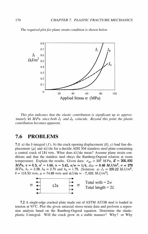
170 CHAPTER 7. PLASTIC FRACTURE MECHANICS
The required plot for plane strain condition is shown below
This plot indicates that the elastic contribution is significant up to approx-imately since both and coincide. Beyond this point the plasticcontribution becomes apparent.
7.1 a) the J-integral ( J ) , b) the crack opening displacement c) load line dis-placement and for a ductile AISI 304 stainless steel plate-containinga central crack of What does mean? Assume plane strain con-ditions and that the stainless steel obeys the Ramberg-Osgood relation at roomtemperature. Explain the results. Given data:
7.2 A single-edge cracked plate made out of ASTM A533B steel is loaded intension at 93°C. Plot the given uniaxial stress-strain data and perform a regres-sion analysis based on the Ramberg-Osgood equation. Determine the elastic-plastic J-integral. Will the crack grow in a stable manner? Why? or Why
7.6 PROBLEMS
and [Solution: a)and ].
not? Assume plane strain conditions and necessary assumptions. Let
[1] J.W. Hutchinson, “Singular Behavior at the End of a Tensile Crack in aHardening Material,” Journal Mech. Phys. Solids, 16(1968) 13-31
[2] J.R. Rice and G.F. Rosengren, “Plane Strain Deformation near a CrackTip in a Power-Law Hardening Material,” Journal Mech. Phys. Sol., 16 (1968)1
[3] K. Hellan, “Introduction to Fracture Mechanics,” McGraw-Hill Bookcompany, New York, (1984)
[4] J.R. Rice, ”A path Independent Integral and the Approximate Analysisof Strain Concentrations by Notches and Cracks,” J. Applied Mech. 35 (1968)379-386
[5] B.S.J. Kang and A.S. Kobayashi, “J-Estimation Procedure based onMoiré Interferometry Data,” Report UWA/DME/TR-87/58, Office of NavalResearch (ONR), (August 1987)
[6] J.W. Dally and W.F. Riley, “Experimental Stress Analysis,” third edi-tion, McGraw-Hill, Inc. New York, (1991)
7.7. REFERENCES 171
0 1.00 2.24 2.30 5.00 7.50 10 20 400 381 414 415 450 469 483 519 557
7.3 Repeat problem 7.2 using the Hollomon equation, for theplastic region. Curve fitting should be performed using this equation for ob-taining K and Assume plane strain conditions and make the necessaryassumptions. Compare the results from Problem 7.2. What can you concludefrom these results? [Solution: a)
7.4 Calculate a) the load-line displacement and b) the crack openingdisplacement which corresponds to a point forUse the following uniaxial data:
7.5 Determine the strain hardening exponent for a steel withAssume that it obeys the Hollomon equation,
with Consider the maximum plastic stress in your calculations.[Solution:
7.6 a) Derive an expression for the J-integral ratio, usingRice model. b) Plot the resultant expression for a remote stress ratio range
Explain the resultant plot.
7.7 REFERENCES
and
[7] J.W. Hutchinson, “Fundamentals of the Phenomenological Theory ofNonlinear Fracture Mechanics,” J. Appl. Mech. 50(1983) 1042-1051
[8] V. Kumar, M.D. German, and C.F. Shih, “An Engineering Approach forElastic-Plastic Fracture Analysis,” General Electric Company, Report Project1237-1, (July 1981)
[9] J.A. Begley and J.D. Landes, American Society for Testing Materials(ASTM), STP 514, (1972)
[10] J.R. Rice, “Mathematical Analysis in the Mechanics of Fracture,” inFracture edited by H. Liebowitz, Vol. II, Academic Press, New York, (1968)191.
[11] J.W. Hutchinson and P.C. Paris, American Society for Testing Materials(ASTM), STP 668, (1979) 37.
[12] C.F. Shih et al., ASTM STP 668, (1979) 65[13] H. Tada et al., “The Stress Analysis of Cracks Handbook,” Del Research
Corporation, Hellertown, PA, (1973)[14] D.P. Rooke and J.C. Cartwright, “Compendium of Stress Intensity Fac-
tors,” Her Majesty’s Stationary Office, London, UK, (1976)[15] G.C. Sih, “Handbook of Stress Intensity Factors,” Inst. of Fracture and
Solid Mechanics, Lehigh University, (1973)[16] V. Kumar and C.F. Shih, “Fully Plastic Crack Solutions, Estimates
Scheme and Stability Analyses for Compact Specimens,” American Society forTesting Materials (ASTM), STP 700, (1980) 406
[17] P.S. Timoshenko and J.N. Goodier, “Theory of Elasticity,” McGraw-HillCo., third edition, (1970)
[18] J.A. Begley et al., ASTM STP 560, (1974) 155.[19] C.F. Shih, “Tables of Hutchinson-Rice-Rosengren Singular Field Quan-
tities,“ Division of Engineering, Brown University, Province, RI, USA, (June1983)
[20] M.S. Dadhah and A.S. Kobayashi, “Further Studies of the HRR Fieldsof a Moving Crack: an Experimental Analysis,” Office of the Chief of NavalResearch, Contract N00014-85-0187, Technical Report No. UWA/DME/TR-88/61, (1988)
[21] A. Saxena, “Nonlinear Fracture Mechanics for Engineers,” CRC PressLLC, New York, (1998) 126.
[22] V. Kumar, M. D. German, and C. F. Shih, “Elastic-Plastic and FullyPlastic Analysis of Crack Initiation, Stable Growth, and Instability in FlawedCylinders,” in Elastic-Plastic Fracture: Second Symposium, ASTM STP 803,Vol. I, (1983) 306-353
[23] M.Y. He and J.W. Hutchinson, “The Penny-Shaped Crack and the PlaneStrain Crack in an Infinite Body of Power-Law Material,” Trans. ASME, J.Applied Mechanics, Vol. 48, (1981) 830-840
[24] M.Y. He and J.W. Hutchinson, “Bounds for Fully Plastic Crack Prob-lems for Infinite Bodies,” ASTM STP 803, Vol. I, (1983) 277-290
[25] H.W. Liu, “On The Fundamentals Basis of Fracture Mechanics,” Eng.Fracture Mech. Vol. 17, No. 5, (1983) 425-438
172 CHAPTER 7. PLASTIC FRACTURE MECHANICS
MIXED-MODEFRACTURE MECHANICS
Practical structures are not only subjected to tension, but also experience shearand torsion loading leading to a mixed-mode interaction. Correspondingly, thestress state ahead of a crack is frequently based on mixed-mode I and II or I andIII type of interactions, which designate the amplitude of the crack-tip stressesbecause of skew-symmetric loading. Problems of this type are encountered inmulti-phase materials such as welded structures, adhesive joints, composite ma-terials, plain and reinforced concrete structures, bridges, aircrafts and so forth.A mixed mode interaction can also arise when crack branching occurs; that is,when a crack changes direction in which the classical energy balance of Griffithcan no longer be carried out in a simple manner since cracking is not collinearas it has been assumed in previous chapters.
In addition, cracks may develop in the skin of aircraft fuselages and canbe subjected to mixed-mode fracture conditions. In general, crack initiationand growth must be correlated with the governing stress intensity factors ina complex state of stress. This means that the crack tip fields are inherentlythree dimensional with varying distribution through the thickness of the solidcomponent. Therefore, the field equations must be determined for a betterunderstanding of mixed-mode fracture mechanics [1-7]. For instance, cracksloaded in tension and shear may exhibit crack branching or kinking can becharacterized using traditional singular and high-order terms in the stress field.The mixed-mode analysis of branched cracks requires the determinations ofstress intensity factors for the original and branched crack parts in terms of thestress field surrounding the crack tip [1-28]. Therefore, an optimal kink angleand the T-stress can be determined based on far-field boundary conditions in ahomogeneous or heterogeneous materials.
Chapter 8
8.1 INTRODUCTION
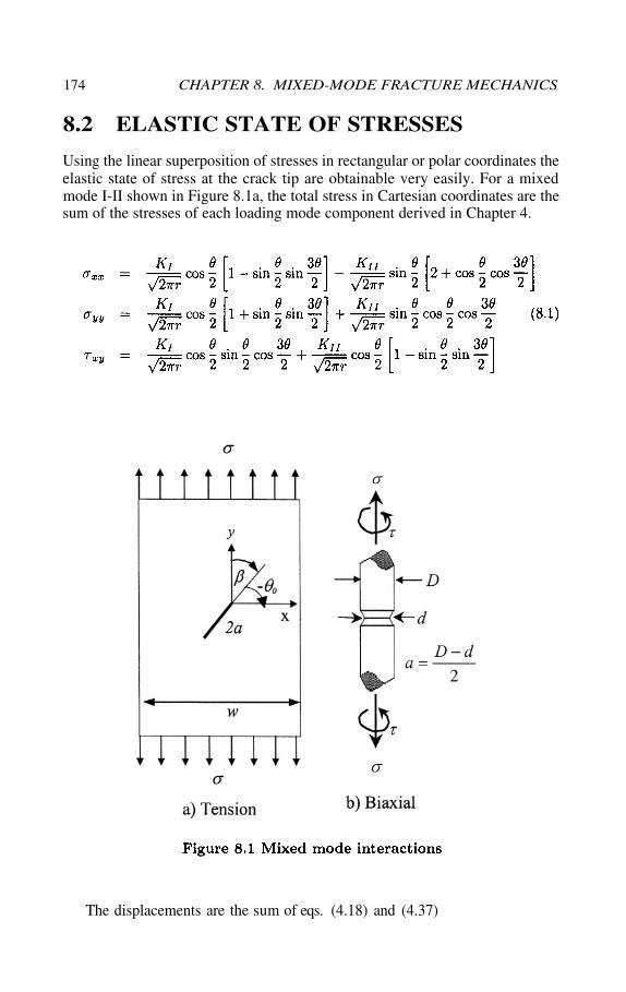
Using the linear superposition of stresses in rectangular or polar coordinates theelastic state of stress at the crack tip are obtainable very easily. For a mixedmode I-II shown in Figure 8.1a, the total stress in Cartesian coordinates are thesum of the stresses of each loading mode component derived in Chapter 4.
The displacements are the sum of eqs. (4.18) and (4.37)
8.2 ELASTIC STATE OF STRESSES
174 CHAPTER 8. MIXED-MODE FRACTURE MECHANICS
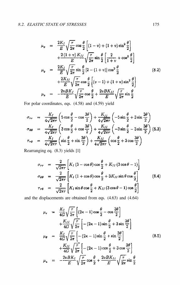
For polar coordinates, eqs. (4.58) and (4.59) yield
Rearranging eq. (8.3) yields [1]
and the displacements are obtained from eqs. (4.63) and (4.64)
8.2. ELASTIC STATE OF STRESSES 175
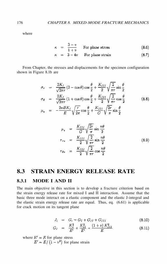
From Chapter, the stresses and displacements for the specimen configurationshown in Figure 8.1b are
The main objective in this section is to develop a fracture criterion based onthe strain energy release rate for mixed I and II interaction. Assume that thebasic three mode interact on a elastic component and the elastic J-integral andthe elastic strain energy release rate are equal. Thus, eq. (6.61) is applicablefor crack motion on its tangent plane
where
8.3 STRAIN ENERGY RELEASE RATE
8.3.1 MODE I AND II
where for plane stressfor plane strain
176 CHAPTER 8. MIXED-MODE FRACTURE MECHANICS
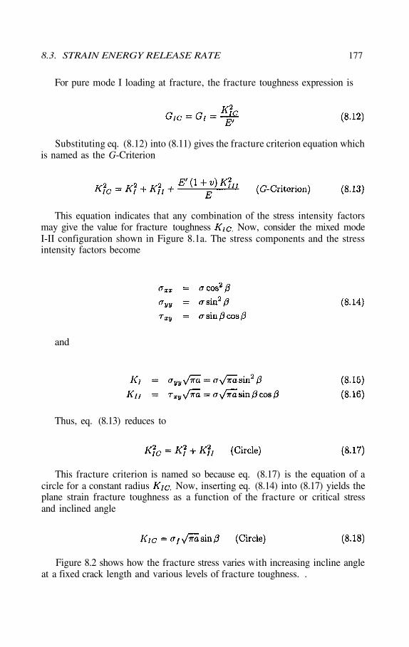
For pure mode I loading at fracture, the fracture toughness expression is
This equation indicates that any combination of the stress intensity factorsmay give the value for fracture toughness Now, consider the mixed modeI-II configuration shown in Figure 8.1a. The stress components and the stressintensity factors become
This fracture criterion is named so because eq. (8.17) is the equation of acircle for a constant radius Now, inserting eq. (8.14) into (8.17) yields theplane strain fracture toughness as a function of the fracture or critical stressand inclined angle
Substituting eq. (8.12) into (8.11) gives the fracture criterion equation whichis named as the G-Criterion
and
Thus, eq. (8.13) reduces to
Figure 8.2 shows how the fracture stress varies with increasing incline angleat a fixed crack length and various levels of fracture toughness. .
8.3. STRAIN ENERGY RELEASE RATE 177
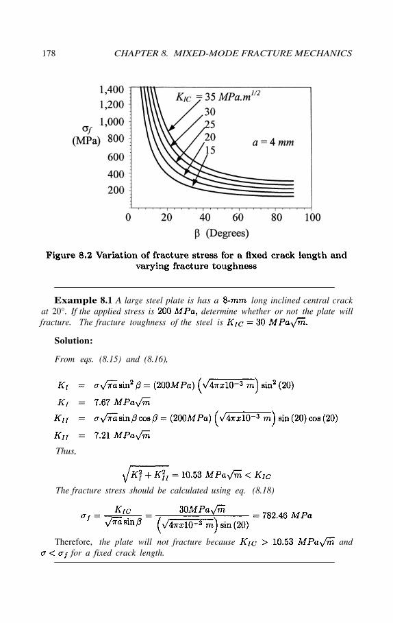
Example 8.1 A large steel plate is has a long inclined central crackat 20°. If the applied stress is determine whether or not the plate willfracture. The fracture toughness of the steel is
Solution:
From eqs. (8.15) and (8.16),
Thus,
The fracture stress should be calculated using eq. (8.18)
Therefore, the plate will not fracture because andfor a fixed crack length.
178 CHAPTER 8. MIXED-MODE FRACTURE MECHANICS
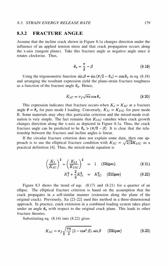
8.3.2 FRACTURE ANGLE
Assume that the incline crack shown in Figure 8.1a changes direction under theinfluence of an applied tension stress and that crack propagation occurs alongthe x-axis (tangent plane). Take this fracture angle as negative angle since itrotates clockwise. Thus,
Using the trigonometric function in eq. (8.18)and arranging the resultant expression yield the plane-strain fracture toughnessas a function of the fracture angle Hence,
This expression indicates that fracture occurs when at a fractureangle for pure mode I loading. Conversely, for pure modeII. Some materials may obey this particular criterion and the mixed-mode eval-uation is very simple. The fact remains that vanishes when crack growthchanges direction along the x-axis as depicted in Figure 8.1a. Thus, the crackfracture angle can be predicted to be It is clear that the rela-tionship between the fracture and incline angles is linear.
If the circular fracture criterion does not explain some data, then one ap-proach is to use the elliptical fracture condition with as apractical definition [4]. Thus, the mixed-mode equation is
Figure 8.3 shows the trend of eqs. (8.17) and (8.21) for a quarter of anellipse. The elliptical fracture criterion is based on the assumption that thecrack propagates in a self-similar manner (extension along the plane of theoriginal crack). Previously, Xu [21-22] used this method in a three-dimensionalapproach. In practice, crack extension in a combined loading system takes placeunder an angle with respect to the original crack plane. This leads to otherfracture theories.
Substituting eq. (8.14) into (8.22) gives
8.3. STRAIN ENERGY RELEASE RATE 179
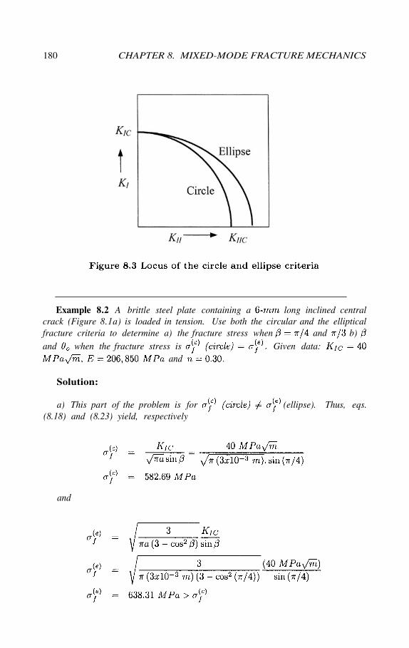
Example 8.2 A brittle steel plate containing a long inclined centralcrack (Figure 8.1a) is loaded in tension. Use both the circular and the ellipticalfracture criteria to determine a) the fracture stress when and b)and when the fracture stress is Given data:
and
and
Solution:
a) This part of the problem is for (ellipse). Thus, eqs.(8.18) and (8.23) yield, respectively
180 CHAPTER 8. MIXED-MODE FRACTURE MECHANICS
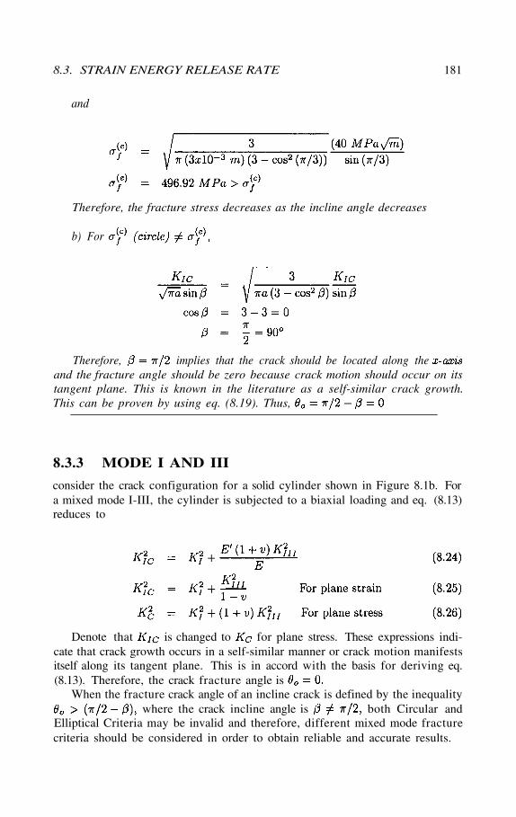
Therefore, implies that the crack should be located along theand the fracture angle should be zero because crack motion should occur on itstangent plane. This is known in the literature as a self-similar crack growth.This can be proven by using eq. (8.19). Thus,
consider the crack configuration for a solid cylinder shown in Figure 8.1b. Fora mixed mode I-III, the cylinder is subjected to a biaxial loading and eq. (8.13)reduces to
Denote that is changed to for plane stress. These expressions indi-cate that crack growth occurs in a self-similar manner or crack motion manifestsitself along its tangent plane. This is in accord with the basis for deriving eq.(8.13). Therefore, the crack fracture angle is
When the fracture crack angle of an incline crack is defined by the inequalitywhere the crack incline angle is both Circular and
Elliptical Criteria may be invalid and therefore, different mixed mode fracturecriteria should be considered in order to obtain reliable and accurate results.
and
Therefore, the fracture stress decreases as the incline angle decreases
8.3.3 MODE I AND III
b) For
8.3. STRAIN ENERGY RELEASE RATE 181
This mixed-mode fracture criterion, has been shown [3,5,6] to beequivalent to the mixed-mode strain energy release rate criterion. This fracturecriterion postulates that crack growth takes place in a direction perpendicularto the maximum principal stress. Hence, the fracture criterion requires that themaximum principal stress be a tension stress for opening the crack along itsplane. This criterion also requires that
Consider the tension loading that produces a mixed-mode I and II interactionas shown in Figure 8.1a and that the stress in eq. (8.4) is a principal stress if
Setting in eq. (8.4) and using eq. (8.15) and (8.16)yield
Using the trigonometric function andin eq. (8.28) and solving for yields
This equation is of practical interest since the fracture angle can be esti-mated knowing value. This fracture angle may be considered asa kink angle in a mixed-mode fracture process in a homogeneous material. Forpure mode II loading, the tension stress intensity factor vanishes andconsequently, eq. (8.28) yields the fracture angle as
The maximum principle stress is defined, after manipulating the trigonomet-ric functions in eq. (8.4), by
8.4 PRINCIPLE STRESS CRITERION
For pure mode I loading at fracture with eq. (8.31) becomes
182 CHAPTER 8. MIXED-MODE FRACTURE MECHANICS
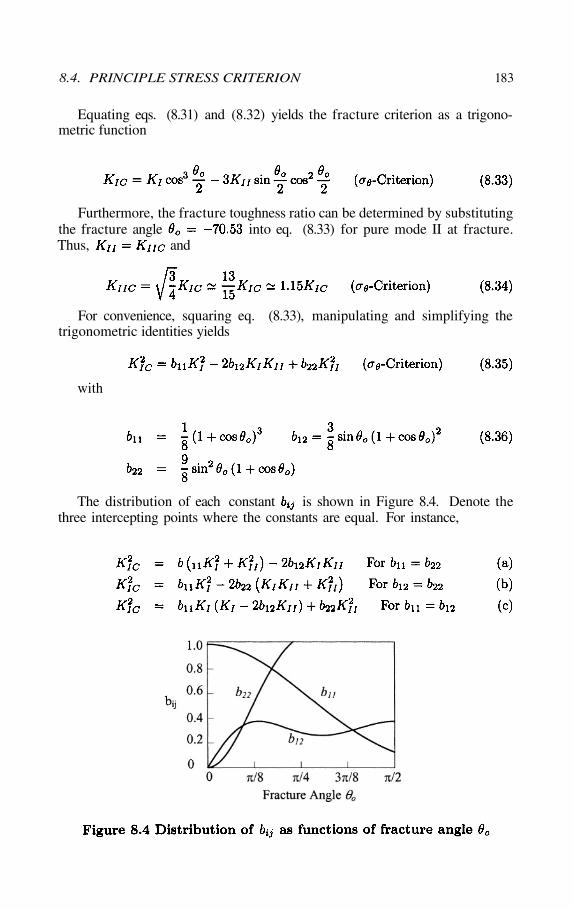
Equating eqs. (8.31) and (8.32) yields the fracture criterion as a trigono-metric function
Furthermore, the fracture toughness ratio can be determined by substitutingthe fracture angle into eq. (8.33) for pure mode II at fracture.Thus, and
with
The distribution of each constant is shown in Figure 8.4. Denote thethree intercepting points where the constants are equal. For instance,
For convenience, squaring eq. (8.33), manipulating and simplifying thetrigonometric identities yields
8.4. PRINCIPLE STRESS CRITERION 183
Sih [2] proposed this criterion using the strain energy density factor (S) for atwo-dimensional stress field. This criterion states that the initial crack growthtakes place in the direction along which the strain-energy-density factor reachesa minimum stationary value so that
This theory can predict crack propagation in an arbitrary direction it statesthat crack propagation occurs when at where is the criticalstrain energy density factor and is the fracture angle.
The development of S-criterion is achieved by inserting the previously de-rived stresses and displacements into the strain energy density equations (withunit thickness). This criterion is related to the work done by the an externalload, which is the stored strain energy density in solids. Thus, eq. (6.58) inrectangular and polar coordinates becomes
Here, V is the volume and is the inner area (region) of the plasticzone model shown Figure 8.5 [2]. This region should not have its sides coincidewith the free crack surface which corresponds to the trivial case when S = 0.
The strain energy density factor is derived by combining eqs. (8.5) and(8.40). Thus,
8.5 STRAIN-ENERGY DENSITY FACTOR
where = constants= Modulus elasticity in shear
E = Modulus elasticity in tension= Poisson’s ratio
184 CHAPTER 8. MIXED-MODE FRACTURE MECHANICS
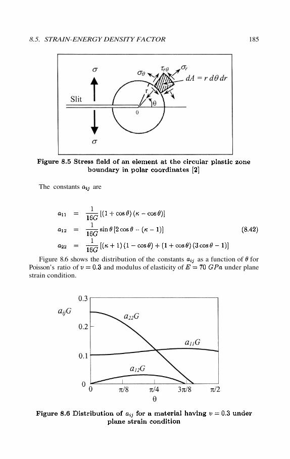
The constants are
Figure 8.6 shows the distribution of the constants as a function of forPoisson’s ratio of and modulus of elasticity of under planestrain condition.
8.5. STRAIN-ENERGY DENSITY FACTOR 185
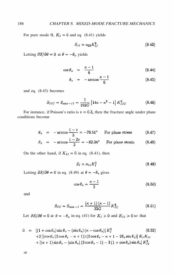
and
For pure mode II, and eq. (8.41) yields
Letting at yields
and eq. (8.43) becomes
For instance, if Poisson’s ratio is then the fracture angle under planeconditions become
On the other hand, if in eq. (8.41), then
Letting in eq. (8.49) at gives
or
186 CHAPTER 8. MIXED-MODE FRACTURE MECHANICS
Let at in eq. (41) for and so that
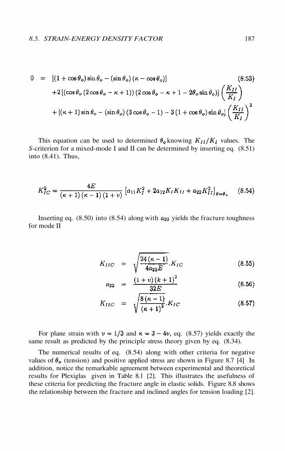
This equation can be used to determined knowing values. TheS-criterion for a mixed-mode I and II can be determined by inserting eq. (8.51)into (8.41). Thus,
Inserting eq. (8.50) into (8.54) along with yields the fracture toughnessfor mode II
For plane strain with and eq. (8.57) yields exactly thesame result as predicted by the principle stress theory given by eq. (8.34).
The numerical results of eq. (8.54) along with other criteria for negativevalues of (tension) and positive applied stress are shown in Figure 8.7 [4] Inaddition, notice the remarkable agreement between experimental and theoreticalresults for Plexiglas given in Table 8.1 [2]. This illustrates the usefulness ofthese criteria for predicting the fracture angle in elastic solids. Figure 8.8 showsthe relationship between the fracture and inclined angles for tension loading [2].
8.5. STRAIN-ENERGY DENSITY FACTOR 187
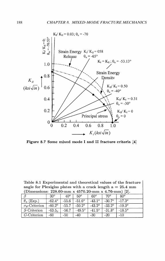
188 CHAPTER 8. MIXED-MODE FRACTURE MECHANICS
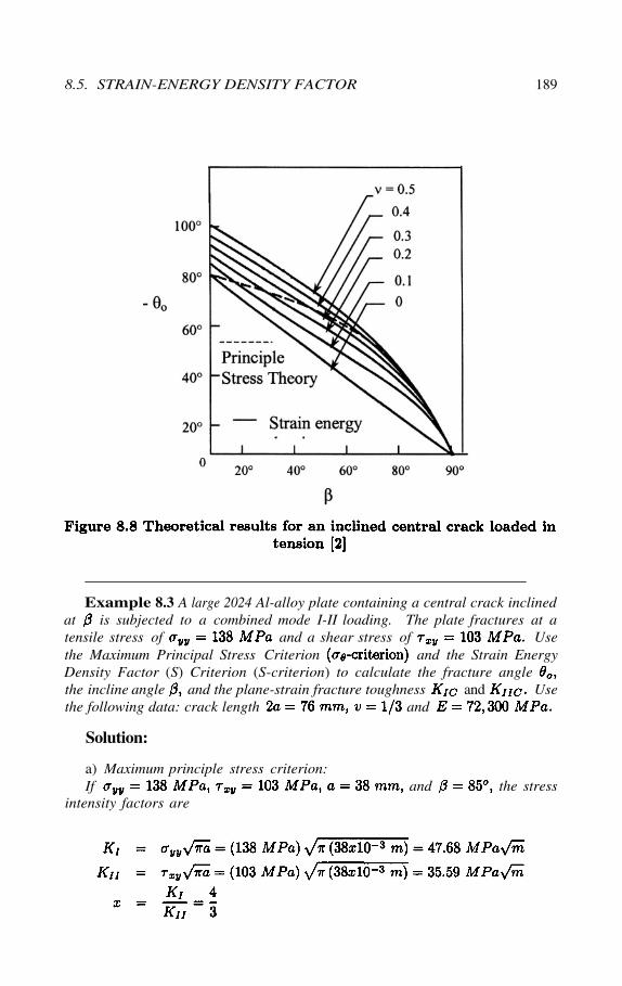
Example 8.3 A large 2024 Al-alloy plate containing a central crack inclinedat is subjected to a combined mode I-II loading. The plate fractures at atensile stress of and a shear stress of Usethe Maximum Principal Stress Criterion and the Strain EnergyDensity Factor (S) Criterion (S-criterion) to calculate the fracture anglethe incline angle and the plane-strain fracture toughness and Usethe following data: crack length and
a) Maximum principle stress criterion:If and the stress
intensity factors are
Solution:
8.5. STRAIN-ENERGY DENSITY FACTOR 189
From eq. (8.29),
The crack is incline at
From eq. (8.34),
b) Strain energy density factor criterion:For plane strain condition,
Inserting the value of and into eq. (8.33) yields
Using eq. (8.53) and an iteration procedure, the fracture angle becomes
190 CHAPTER 8. MIXED-MODE FRACTURE MECHANICS
and
Finally, the fracture toughness for mode II and the critical strain energydensity factor are
and
Therefore, crack propagation takes place when at
From eq. (8.42) and (8.54),
8.5. STRAIN-ENERGY DENSITY FACTOR 191
8.6 CRACK BRANCHING
It is recognized that the tensile cracks in solids can significantly branch due tomechanical, microstructural or environmental effects. Changes in crack pathare normally induced by [7-12]
1) Multiaxial far field stresses
2) Interaction of the crack tip with microstructural defects
3) Sudden changes in load
4) The embrittlement effect of an aggressive environment
Figure 8.9 illustrates some examples of severely branched cracks in ductilematerials during different conditions, which can be found in the cited references.The effects of crack branching can be rationalized based on the stress intensityfactors for the small-branched cracks shown in Figure 8.10. However, numeroussolutions for kinked and forked cracks have been proposed, but there have beenconsiderable disagreements.
The stress intensity factors and for kinked and forked cracks aresmaller than the nominal and Based on the projected length of thecrack, and are meaningful if the plastic zone is smaller than the zone ofdominance of the and singular fields.
The stress intensity factor solutions for kinked and forked elastic cracks undermixed mode I-II loading are based on the models shown in Figure 8.10 [7,13-16].Thus,
where are defined as
192 CHAPTER 8. MIXED-MODE FRACTURE MECHANICS
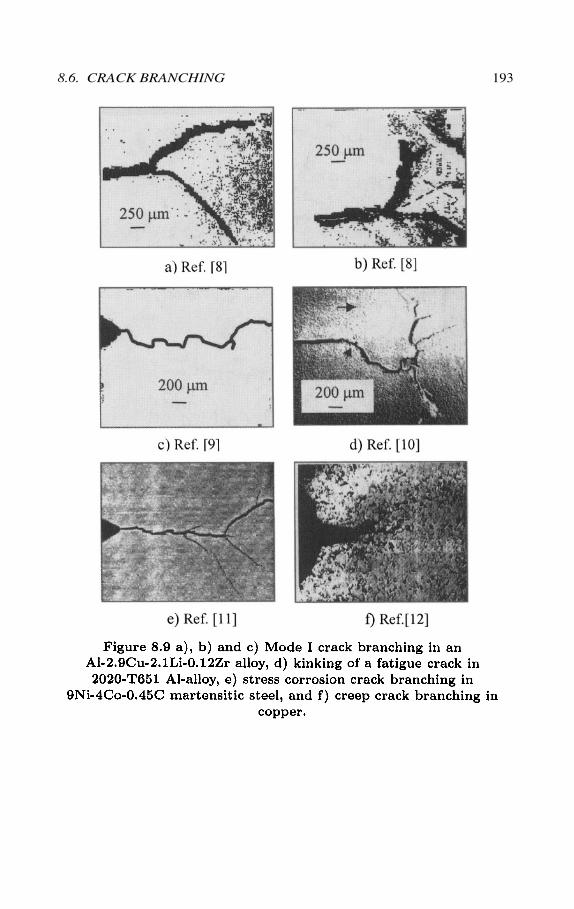
8.6. CRACK BRANCHING 193
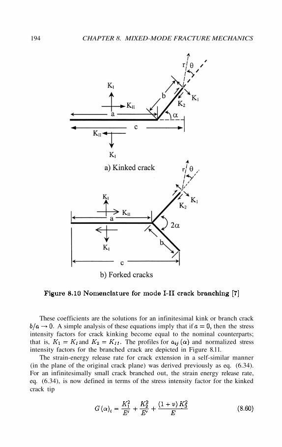
These coefficients are the solutions for an infinitesimal kink or branch crackA simple analysis of these equations imply that if then the stress
intensity factors for crack kinking become equal to the nominal counterparts;that is, and The profiles for and normalized stressintensity factors for the branched crack are depicted in Figure 8.11.
The strain-energy release rate for crack extension in a self-similar manner(in the plane of the original crack plane) was derived previously as eq. (6.34).For an infinitesimally small crack branched out, the strain energy release rate,eq. (6.34), is now defined in terms of the stress intensity factor for the kinkedcrack tip
194 CHAPTER 8. MIXED-MODE FRACTURE MECHANICS
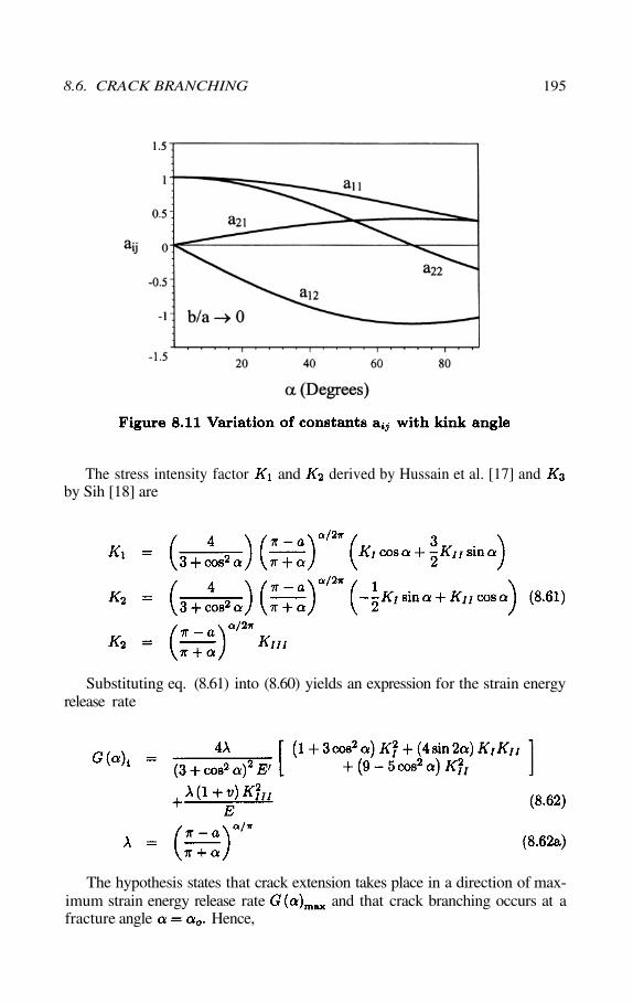
The stress intensity factor and derived by Hussain et al. [17] andby Sih [18] are
Substituting eq. (8.61) into (8.60) yields an expression for the strain energyrelease rate
The hypothesis states that crack extension takes place in a direction of max-imum strain energy release rate and that crack branching occurs at afracture angle Hence,
8.6. CRACK BRANCHING 195
Crack propagation takes place when For pure mode I atfracture, eq. (8.62) becomes
Letting in eq. (8.62) yields the fracture criterion
[8.1] A large plate (2024-0 Al-alloy) containing a central crack is subjected toa combined mode I-II loading. The internal stresses are and
Use the maximum principal stress criterion tocalculate the fracture toughness ( and ). Data: crack length
and [Solution: and
[8.2] Repeat problem 8.1 using the strain energy density factor criterion(S-criterion).
Denote that if in eqs. (8.62) and (8.65), the former reduces to eq.(6.34) and the latter becomes eq. (8.13).
Furthermore, the above mathematical treatment of mixed-mode fracture me-chanics problems has been based on the stress field surrounding the crack tipwhere stress singularities exists as Including the influence of the T-stress in the mixed mode I and II process, the generalized stress based onWilliams [23] K-field solution for unkinked crack is defined as [24]
Recall from Chapter 4 that is a second order term in the series expan-sion of the stress field and it is non-singular, but specimen size and geometrydependent. As pointed out by Becker et al. [24], represents the strength inthe crack x-direction. For mode I loading, and for stabilizingthe crack. Conversely, crack branching may occur when and atangle as indicated in Figure 8.10. Further theoretical or numerical details oncrack kinking can be found elsewhere [25-28].
8.7 PROBLEMS
196 CHAPTER 8. MIXED-MODE FRACTURE MECHANICS
[8.3] Determine a) the applied tensile stress and b) the safety factor for aloaded plate containing a central crack inclined at 53.25°. The strainenergy release rate mode I is Data:
and [Solution: and SF = 4.46].
[1] G.C. Sih and H. Liebowitz, “Mathematical Fundamental of Fracture,”Academic Press, New York, (1968) 67-190
[2] G.C. Sih, Inter. J. Fracture, 10(3) (1974) 305 - 321.[3] G.C. Sih, P.C. Paris and F. Erdogan, Inter. J. Fracture Mech., 29(1962)
306-312[4] R.W. Hertzberg, “Deformation and Fracture Mechanics of Engineering
Materials,” Third edition, John Wiley & Sons, New York, (1989)[5] F. Erdogan and G.C. Sih, “On The Crack Extension in Plates Under
Plane Loading and Transverse Shear,” J. Basic Eng., 85(1963) 519-527[6] R.J. Nuismer, Inter. Journal of Fracture, 11(1975) 245-250[7] S. Suresh and C.F. Shin, Inter J. Fracture, 30 (1986) 237-259[8] A.K. Vasudevan and S. Suresh, Mat. Sci. Eng. 72 (1985) 37-49[9] S. Suresh, Met. Trans. 16A (1985) 249-260[10] C.H. Wu, J. Applied Mechanics, 45 (1978) 553-558[11] C.S. Carter, Eng. Fract. Mech. 3(1971) 1-13[12] D.R. Hayhurst, P.R. Brown and C.J. Morrison, Philosophical Transac-
tions Royal Society London, A 311 (1984) 131-158[13] Z. Yishu, Eng. Fracture Mech. Vol. 26, No. 5 (1987) 683-689[14] B. Cottrell and J.R. Rice, Inter. J. Fracture 16 (1980) 155-169[15] B.A. Bilby, G.E. Cardew and I.C. Howard, in fracture 1977, ed. by
D.M.R. Taplin, Vol. 3, University of Waterloo Press (1977) 197-200[16] H. Kitagawa, R. Yuki and T. Ohira, Eng. Fract. Mech. 7(1975) 515-529[17] M.A. Hussain, S.L. Pu and J. Underwood, ASTM STP 560, (1973) 2-28.[18] G.C. Sih, J. Appl. Mech. 32 (1965) 51-58[19] K. Palaniswamy, Ph.D. Thesis, California Institute of Technology, (1972)[20] B.C. Hoskin, D.G. Graff and P.J. Foden, Aer. Res. Lab., Melbourne,
Report S.M. 305 (1965)
8.8 REFERENCES
[8.4] Calculate the critical stress (fracture stress) for the problem describedin problem 8.3 according to the Will crack propagation take place?
[8.5] Repeat problem 8.4 using the S-criterion with [Solution:
[8.6] Show that the stress intensity factor is when
and the Poisson’s ration is
8.8. REFERENCES 197
[21] Y. Xu, B. Moran, and T. Belytschko, Trans. ASME, J. Applied Me-chanics, Vol. 65, (Sept. 1998) 557-565
[22] Y. Xu, Engineering Fracture Mechanics, Vol. 59, 2 (1999)[23] M.L. Williams, “On The Stress Distribution At The Base Of A Station-
ary Crack,” J. Appl. Mech., 24 (1957) 109-114[24] T.L. Becker Jr., R.M. Cannon and R.O. Ritchie, “Finite Crack Kinking
and T-stresses in Functionally Graded Materials,” Inter. Journal of Solids andStructures, 38 (2001) 5545-5563
[25] B. Cotterell, “Notes on the Paths and Instability of Cracks,” Inter.Journal of Fracture, 2 (1966) 526-533
[26] M.Y. He and J.W. Hutchinson, “Kinking of a Crack out of an Interface,”J. Applied Mechanics, 56 (1989) 270-278
[27] M.Y. He, A. Bartlett, A. Evans and J.W. Hutchinson, “Kinking of aCrack out of an Interface: Role of Plane Stress,” J. Am. Ceram. Soc., 74(1991) 767-771
[28] K. Palaniswamy and W.G. Knauss, “On the Problem of Crack Ex-tension in Brittle Solids under general loading,” in S. Namat-Nassar editor,Mechanics Today, Pergamon Press, New York, Vol. 4 (1978)
198 CHAPTER 8. MIXED-MODE FRACTURE MECHANICS
Chapter 9
FATIGUE CRACKGROWTH
9.1 INTRODUCTION
Fatigue in materials subjected to repeated cyclic loading can be defined as aprogressive failure due to crack initiation (stage I), crack growth (stage II), andcrack propagation (stage III) or instability stage. For instance, crack initiation ofcrack-free solids may be characterized by fatigue crack nuclei due to dislocationmotion, which generates slip bands at the surface having slip steps in the orderof in height [1-2] or slip may occur at matrix-inclusion interfaces. Thesesteps produce surface intrusions and extrusions as schematically indicate belowfor stages I and II. These intrusions caused by reversed slip due to load reversalare the source for crack initiation, which may consume most of the solid lifebefore crack growth. This crack initiation may occur along the slip directiondue to a local maximum shear stress. After the consumption of many cycles,the crack may change in direction when the maximum principal normal stress(in the vicinity of the crack tip) governs crack growth. In this stage II somematerials show striations and beach marks as common surface features of fatiguefracture.
In general, fatigue is a form of failure caused by fluctuating or cyclic loadsover a short or prolong period of time. Therefore, fatigue is a time-dependentfailure mechanism related to microstructural features. The fluctuating loadingcondition is not a continuous failure process as opposed to cyclic loading. Theformer is manifested in bridges, aircrafts and machine components, while thelatter requires a continuous constant or variable stress amplitude until fractureoccurs. It is also important for the reader to know that fatigue failure or fracturecan occur at a maximum stress below the static yield strength of a particularmaterial. Obviously, temperature effects must be considered in fatigue failurecharacterization. From an engineering point of view, predicting fatigue life ismajor a requirement.
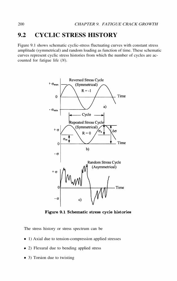
9.2 CYCLIC STRESS HISTORY
Figure 9.1 shows schematic cyclic-stress fluctuating curves with constant stressamplitude (symmetrical) and random loading as function of time. These schematiccurves represent cyclic stress histories from which the number of cycles are ac-counted for fatigue life (N).
The stress history or stress spectrum can be
1) Axial due to tension-compression applied stresses
2) Flexural due to bending applied stress
3) Torsion due to twisting
200 CHAPTER 9. FATIGUE CRACK GROWTH
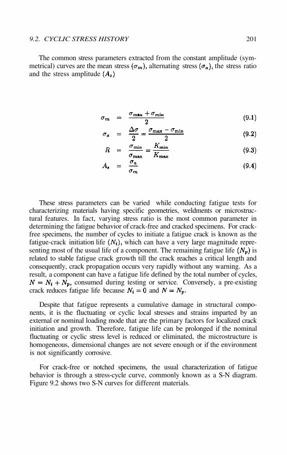
The common stress parameters extracted from the constant amplitude (sym-metrical) curves are the mean stress alternating stress the stress ratioand the stress amplitude
These stress parameters can be varied while conducting fatigue tests forcharacterizing materials having specific geometries, weldments or microstruc-tural features. In fact, varying stress ratio is the most common parameter indetermining the fatigue behavior of crack-free and cracked specimens. For crack-free specimens, the number of cycles to initiate a fatigue crack is known as thefatigue-crack initiation life which can have a very large magnitude repre-senting most of the usual life of a component. The remaining fatigue life isrelated to stable fatigue crack growth till the crack reaches a critical length andconsequently, crack propagation occurs very rapidly without any warning. As aresult, a component can have a fatigue life defined by the total number of cycles,
consumed during testing or service. Conversely, a pre-existingcrack reduces fatigue life because and
Despite that fatigue represents a cumulative damage in structural compo-nents, it is the fluctuating or cyclic local stresses and strains imparted by anexternal or nominal loading mode that are the primary factors for localized crackinitiation and growth. Therefore, fatigue life can be prolonged if the nominalfluctuating or cyclic stress level is reduced or eliminated, the microstructure ishomogeneous, dimensional changes are not severe enough or if the environmentis not significantly corrosive.
For crack-free or notched specimens, the usual characterization of fatiguebehavior is through a stress-cycle curve, commonly known as a S-N diagram.Figure 9.2 shows two S-N curves for different materials.
9.2. CYCLIC STRESS HISTORY 201
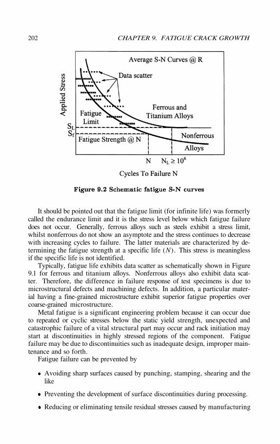
It should be pointed out that the fatigue limit (for infinite life) was formerlycalled the endurance limit and it is the stress level below which fatigue failuredoes not occur. Generally, ferrous alloys such as steels exhibit a stress limit,whilst nonferrous do not show an asymptote and the stress continues to decreasewith increasing cycles to failure. The latter materials are characterized by de-termining the fatigue strength at a specific life (N). This stress is meaninglessif the specific life is not identified.
Typically, fatigue life exhibits data scatter as schematically shown in Figure9.1 for ferrous and titanium alloys. Nonferrous alloys also exhibit data scat-ter. Therefore, the difference in failure response of test specimens is due tomicrostructural defects and machining defects. In addition, a particular mater-ial having a fine-grained microstructure exhibit superior fatigue properties overcoarse-grained microstructure.
Metal fatigue is a significant engineering problem because it can occur dueto repeated or cyclic stresses below the static yield strength, unexpected andcatastrophic failure of a vital structural part may occur and rack initiation maystart at discontinuities in highly stressed regions of the component. Fatiguefailure may be due to discontinuities such as inadequate design, improper main-tenance and so forth.
Fatigue failure can be prevented by
Avoiding sharp surfaces caused by punching, stamping, shearing and thelike
Preventing the development of surface discontinuities during processing.
Reducing or eliminating tensile residual stresses caused by manufacturing
202 CHAPTER 9. FATIGUE CRACK GROWTH
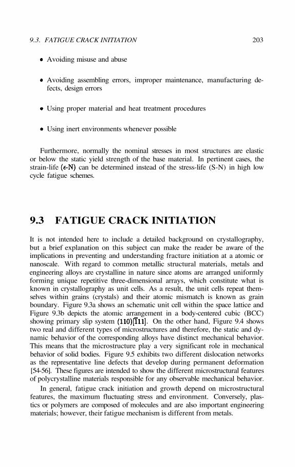
Avoiding misuse and abuse
Avoiding assembling errors, improper maintenance, manufacturing de-fects, design errors
Using proper material and heat treatment procedures
Using inert environments whenever possible
Furthermore, normally the nominal stresses in most structures are elasticor below the static yield strength of the base material. In pertinent cases, thestrain-life can be determined instead of the stress-life (S-N) in high lowcycle fatigue schemes.
9.3 FATIGUE CRACK INITIATION
It is not intended here to include a detailed background on crystallography,but a brief explanation on this subject can make the reader be aware of theimplications in preventing and understanding fracture initiation at a atomic ornanoscale. With regard to common metallic structural materials, metals andengineering alloys are crystalline in nature since atoms are arranged uniformlyforming unique repetitive three-dimensional arrays, which constitute what isknown in crystallography as unit cells. As a result, the unit cells repeat them-selves within grains (crystals) and their atomic mismatch is known as grainboundary. Figure 9.3a shows an schematic unit cell within the space lattice andFigure 9.3b depicts the atomic arrangement in a body-centered cubic (BCC)showing primary slip system On the other hand, Figure 9.4 showstwo real and different types of microstructures and therefore, the static and dy-namic behavior of the corresponding alloys have distinct mechanical behavior.This means that the microstructure play a very significant role in mechanicalbehavior of solid bodies. Figure 9.5 exhibits two different dislocation networksas the representative line defects that develop during permanent deformation[54-56]. These figures are intended to show the different microstructural featuresof polycrystalline materials responsible for any observable mechanical behavior.
In general, fatigue crack initiation and growth depend on microstructuralfeatures, the maximum fluctuating stress and environment. Conversely, plas-tics or polymers are composed of molecules and are also important engineeringmaterials; however, their fatigue mechanism is different from metals.
9.3. FATIGUE CRACK INITIATION 203
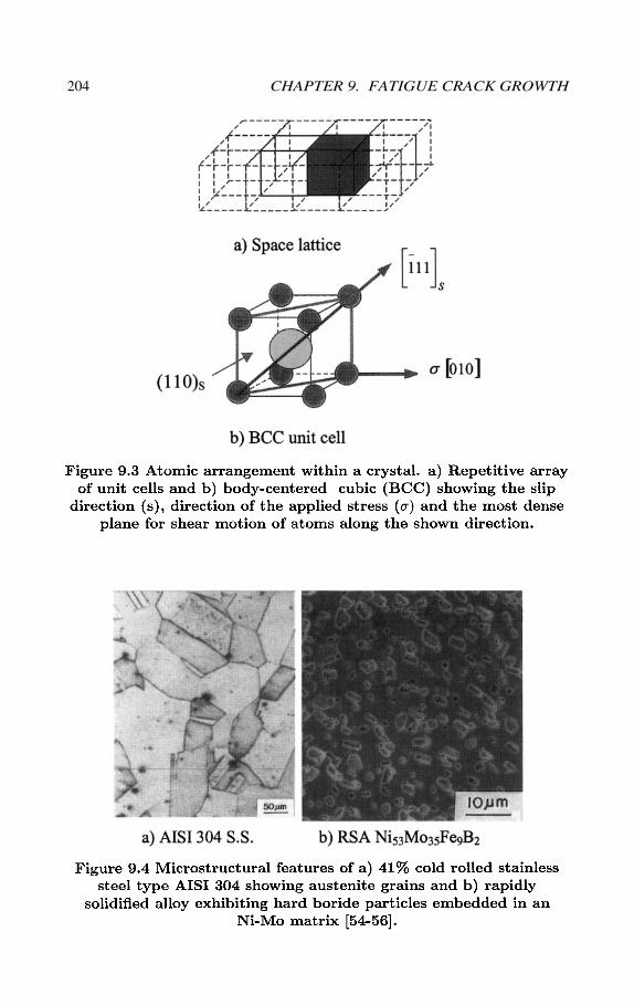
204 CHAPTER 9. FATIGUE CRACK GROWTH
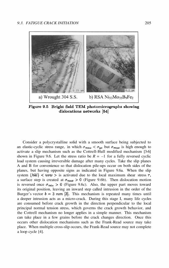
Consider a polycrystalline solid with a smooth surface being subjected toan elastic-cyclic stress range, in which but is high enough toactivate a slip mechanism such as the Cottrell-Hull modified mechanism [3-6]shown in Figure 9.6. Let the stress ratio be R = –1 for a fully reversed cyclicload system causing irreversible damage after many cycles. Take the slip planesA and B for convenience so that dislocation pile-ups occur on both sides of theplanes, but having opposite signs as indicated in Figure 9.6a. When the slipsystem is activated due to the local maximum shear stressa surface step is created at (Figure 9.6b). Then dislocation motionis reversed once (Figure 9.6c). Also, the upper part moves towardits original position, leaving an inward step called intrusion in the order of theBurger’s vector This mechanism is repeated many times untila deeper intrusion acts as a micro-crack. During this stage I, many life cyclesare consumed before crack growth in the direction perpendicular to the localprincipal normal tension stress, which governs the crack growth behavior, andthe Cottrell mechanism no longer applies in a simple manner. This mechanismcan take place in a few grains before the crack changes direction. Once thisoccurs other dislocation mechanisms such as the Frank-Read source may takeplace. When multiple cross-slip occurs, the Frank-Read source may not completea loop cycle [4].
9.3. FATIGUE CRACK INITIATION 205
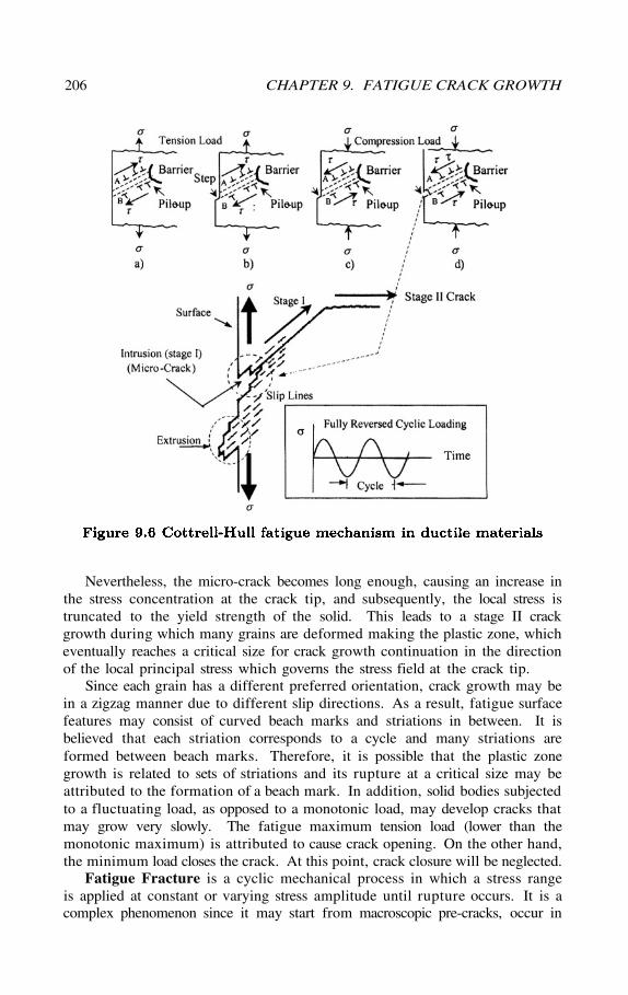
Nevertheless, the micro-crack becomes long enough, causing an increase inthe stress concentration at the crack tip, and subsequently, the local stress istruncated to the yield strength of the solid. This leads to a stage II crackgrowth during which many grains are deformed making the plastic zone, whicheventually reaches a critical size for crack growth continuation in the directionof the local principal stress which governs the stress field at the crack tip.
Since each grain has a different preferred orientation, crack growth may bein a zigzag manner due to different slip directions. As a result, fatigue surfacefeatures may consist of curved beach marks and striations in between. It isbelieved that each striation corresponds to a cycle and many striations areformed between beach marks. Therefore, it is possible that the plastic zonegrowth is related to sets of striations and its rupture at a critical size may beattributed to the formation of a beach mark. In addition, solid bodies subjectedto a fluctuating load, as opposed to a monotonic load, may develop cracks thatmay grow very slowly. The fatigue maximum tension load (lower than themonotonic maximum) is attributed to cause crack opening. On the other hand,the minimum load closes the crack. At this point, crack closure will be neglected.
Fatigue Fracture is a cyclic mechanical process in which a stress rangeis applied at constant or varying stress amplitude until rupture occurs. It is acomplex phenomenon since it may start from macroscopic pre-cracks, occur in
206 CHAPTER 9. FATIGUE CRACK GROWTH
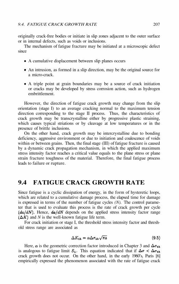
originally crack-free bodies or initiate in slip zones adjacent to the outer surfaceor in internal defects, such as voids or inclusions.
The mechanism of fatigue fracture may be initiated at a microscopic defectsince
A cumulative displacement between slip planes occurs
An intrusion, as formed in a slip direction, may be the original source fora micro-crack.
A triple point at grain boundaries may be a source of crack initiationor cracks may be developed by stress corrosion action, such as hydrogenembrittlement.
However, the direction of fatigue crack growth may change from the sliporientation (stage I) to an average cracking normal to the maximum tensiondirection corresponding to the stage II process. Thus, the characteristics ofcrack growth may be transcrystalline either by progressive plastic straining,which causes typical striations or by cleavage at low temperatures or in thepresence of brittle inclusions.
On the other hand, crack growth may be intercrystalline due to bondingdeficiency, aggressive environment or due to initiation and coalescence of voidswithin or between grains. Then, the final stage (III) of fatigue fracture is causedby a dynamic crack propagation mechanism, in which the applied maximumstress intensity factor reaches a critical value equals to the plane stress or planestrain fracture toughness of the material. Therefore, the final fatigue processleads to failure or rupture.
9.4 FATIGUE CRACK GROWTH RATE
Since fatigue is a cyclic dissipation of energy, in the form of hysteretic loops,which are related to a cumulative damage process, the elapsed time for damageis expressed in terms of the number of fatigue cycles (N). The control parame-ter that is used to evaluate this process is the rate of crack growth per cycle
Hence, depends on the applied stress intensity factor rangeand N is the well-known fatigue life term.
For crack initiation or stage I, the threshold stress intensity factor and thresh-old stress range are associated as
Here, is the geometric correction factor introduced in Chapter 3 andis analogous to fatigue limit This equation indicated that ifcrack growth does not occur. On the other hand, in the early 1960’s, Paris [6]empirically expressed the phenomenon associated with the rate of fatigue crack
9.4. FATIGUE CRACK GROWTH RATE 207
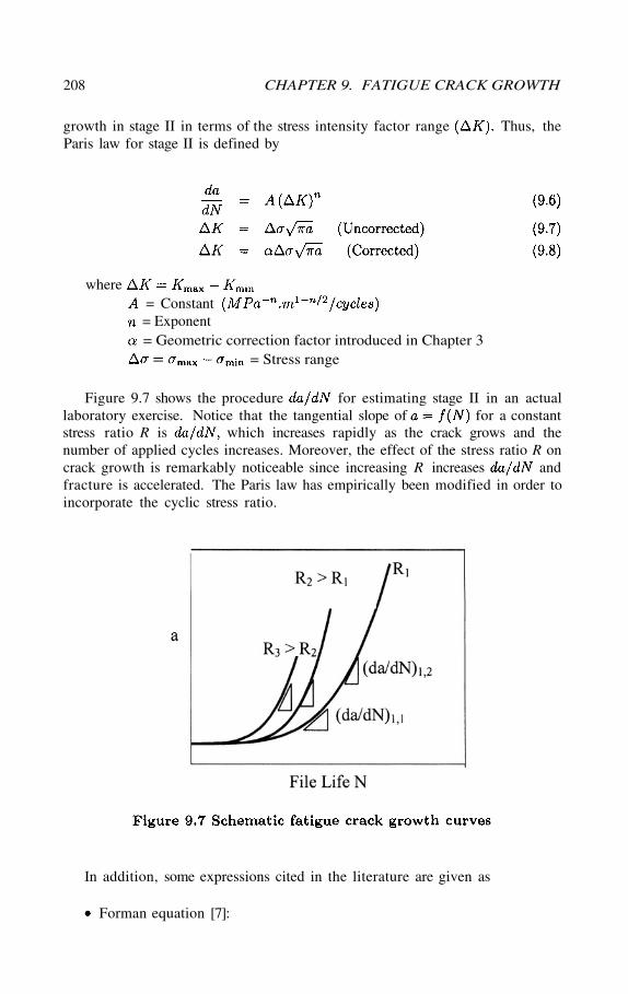
growth in stage II in terms of the stress intensity factor range Thus, theParis law for stage II is defined by
Figure 9.7 shows the procedure for estimating stage II in an actuallaboratory exercise. Notice that the tangential slope of for a constantstress ratio R is which increases rapidly as the crack grows and thenumber of applied cycles increases. Moreover, the effect of the stress ratio R oncrack growth is remarkably noticeable since increasing R increases andfracture is accelerated. The Paris law has empirically been modified in order toincorporate the cyclic stress ratio.
In addition, some expressions cited in the literature are given as
Forman equation [7]:
208 CHAPTER 9. FATIGUE CRACK GROWTH
whereA = Constant
= Exponent= Geometric correction factor introduced in Chapter 3
= Stress range
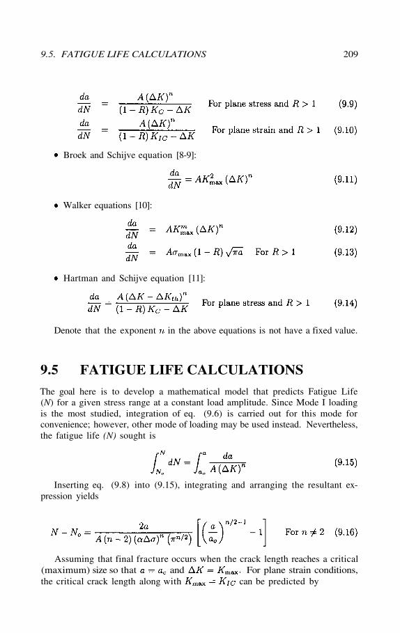
Broek and Schijve equation [8-9]:
Walker equations [10]:
Hartman and Schijve equation [11]:
Denote that the exponent in the above equations is not have a fixed value.
9.5 FATIGUE LIFE CALCULATIONS
The goal here is to develop a mathematical model that predicts Fatigue Life(N) for a given stress range at a constant load amplitude. Since Mode I loadingis the most studied, integration of eq. (9.6) is carried out for this mode forconvenience; however, other mode of loading may be used instead. Nevertheless,the fatigue life (N) sought is
Inserting eq. (9.8) into (9.15), integrating and arranging the resultant ex-pression yields
Assuming that final fracture occurs when the crack length reaches a critical(maximum) size so that and For plane strain conditions,the critical crack length along with can be predicted by
9.5. FATIGUE LIFE CALCULATIONS 209
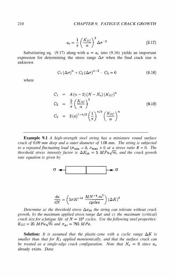
Substituting eq. (9.17) along with into (9.16) yields an importantexpression for determining the stress range when the final crack size isunknown
where
Example 9.1 A high-strength steel string has a miniature round surfacecrack of 0.09 mm deep and a outer diameter of 1.08 mm. The string is subjectedto a repeated fluctuating load at a stress ratio R = 0. Thethreshold stress intensity factor is and the crack growthrate equation is given by
Determine a) the threshold stress the string can tolerate without crackgrowth, b) the maximum applied stress range and c) the maximum (critical)crack size for a fatigue life of cycles. Use the following steel properties:
and
Solution: It is assumed that the plastic-zone with a cyclic range issmaller than that for applied monotonically, and that the surface crack canbe treated as a single-edge crack configuration. Note that sincealready exists. Data:
210 CHAPTER 9. FATIGUE CRACK GROWTH
a) From eqs. (3.56),
Thus, eqs. (3.54) and (9.5) yield respectively
b) Use eq. (9.19) and subsequently (9.18) to get
and
Solving the above biquadratic equation yields four roots. The positive root is
9.5. FATIGUE LIFE CALCULATIONS 211
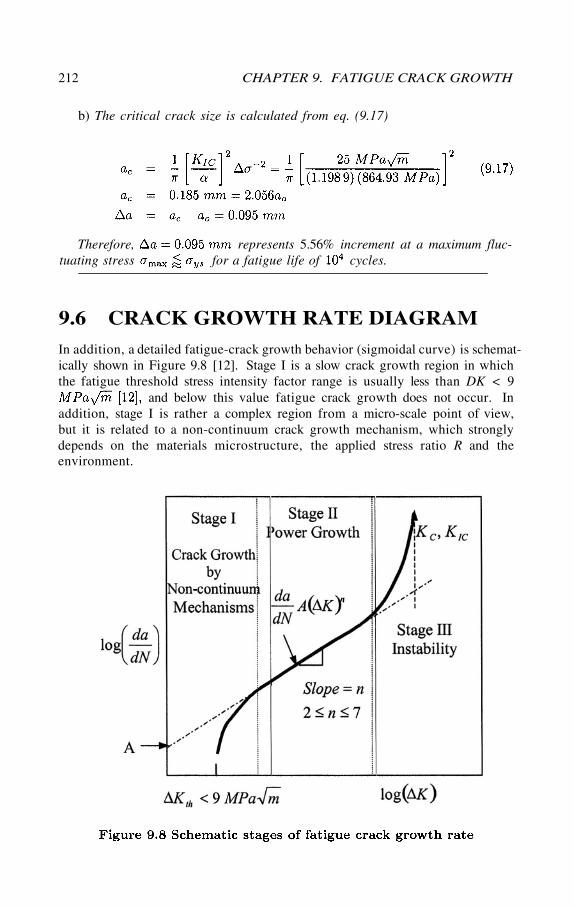
b) The critical crack size is calculated from eq. (9.17)
Therefore, represents 5.56% increment at a maximum fluc-tuating stress for a fatigue life of cycles.
9.6 CRACK GROWTH RATE DIAGRAM
In addition, a detailed fatigue-crack growth behavior (sigmoidal curve) is schemat-ically shown in Figure 9.8 [12]. Stage I is a slow crack growth region in whichthe fatigue threshold stress intensity factor range is usually less than DK < 9
and below this value fatigue crack growth does not occur. Inaddition, stage I is rather a complex region from a micro-scale point of view,but it is related to a non-continuum crack growth mechanism, which stronglydepends on the materials microstructure, the applied stress ratio R and theenvironment.
212 CHAPTER 9. FATIGUE CRACK GROWTH
ANALYSIS OF Figure 9.8:Stage I: This is a slow crack growth process which is related to non-
continuum mechanisms and slow fatigue crack growth in the order ofThus, this fatigue process strongly depends on the
a) Microstructural parameters such as grain size, precipitates, dislocationdensity, etc.
b) Mean tress and stress ratio
c) Aggressiveness of the environment
d) Surface damage initiation
Stage II: This fatigue process is referred to as the power growth behaviorusually characterized by the Paris law and it slightly depends on the parametersin stage I. Particularly, surface characteristics are the formation of beach marksand striations in some metallic materials. Furthermore, the specimen thicknessdoes not strongly influence the fatigue crack growth rate.
Striations are microscopic fatigue features that can be observed with thescanning electron microscope (SEM) and the transmission electron microscope(TEM) at relatively high magnifications. Conversely, each striation indicatesa successive advance of one stress cycle. The width of a striation representsthe advance of the crack front during one stress cycle, but it depends on themagnitude of the applied stress range. Normally, the appearance of servicefatigue striations is irregular due to changeable stress amplitude. Striation aredealt with in later section. Then, this irregularity in striation configurationis an indication of non-steady crack growth rate, which may be restricted togeometry-dependency and load history, leading to an enhanced or retarded rate.
Stage III: This fatigue process strongly depends on the microstructuralparameters cited in stage I and on the specimen thickness. Since the appliedstress intensity factor is sufficiently large, the fatigue crack growth is high andthe process is under an instable damage process. Therefore, this is the instabilityregion in Figure 9.8 and fracture occurs when the stress intensity factor reachesa critical value.
Figure 9.9 schematically shows the influence of R on stage I [13]. Figure9.10 depicts experimental for a structural steel [14] Forinstance, the most common engineering metallic materials have a BCC, FCC,or HCP atomic structure; therefore, the fatigue behavior of these materials isexpected to be different. Generally, surface crack initiation occurs in this State Iin which the crack growth rate is very slow. In addition, stage II is known as thepower crack growth, which is less dependent on the microstructure, stress ratio,and environment than stage I. The log-log linear fatigue behavior is referred toas the Paris Law, which empirically define by eq. (9.6). The characteristics ofthe surface fracture appearance may include beach marks and striations thatare observable in certain materials such aluminum and aluminum alloys. Both
9.6. CRACK GROWTH RATE DIAGRAM 213
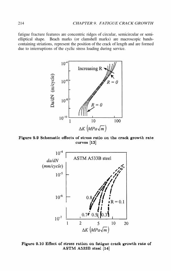
fatigue fracture features are concentric ridges of circular, semicircular or semi-elliptical shape. Beach marks (or clamshell marks) are macroscopic bands-containing striations, represent the position of the crack of length and are formeddue to interruptions of the cyclic stress loading during service.
214 CHAPTER 9. FATIGUE CRACK GROWTH
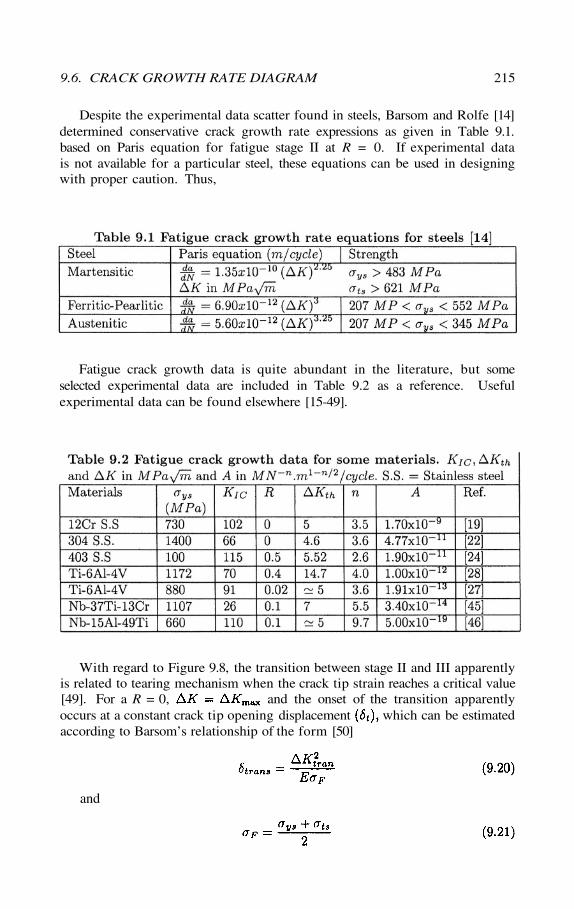
Despite the experimental data scatter found in steels, Barsom and Rolfe [14]determined conservative crack growth rate expressions as given in Table 9.1.based on Paris equation for fatigue stage II at R = 0. If experimental datais not available for a particular steel, these equations can be used in designingwith proper caution. Thus,
Fatigue crack growth data is quite abundant in the literature, but someselected experimental data are included in Table 9.2 as a reference. Usefulexperimental data can be found elsewhere [15-49].
With regard to Figure 9.8, the transition between stage II and III apparentlyis related to tearing mechanism when the crack tip strain reaches a critical value[49]. For a R = 0, and the onset of the transition apparentlyoccurs at a constant crack tip opening displacement which can be estimatedaccording to Barsom’s relationship of the form [50]
and
9.6. CRACK GROWTH RATE DIAGRAM 215
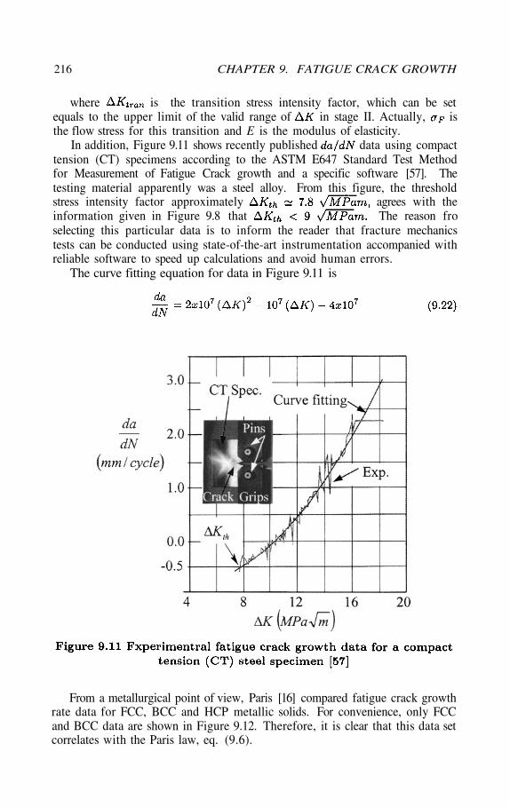
where is the transition stress intensity factor, which can be setequals to the upper limit of the valid range of in stage II. Actually, isthe flow stress for this transition and E is the modulus of elasticity.
In addition, Figure 9.11 shows recently published data using compacttension (CT) specimens according to the ASTM E647 Standard Test Methodfor Measurement of Fatigue Crack growth and a specific software [57]. Thetesting material apparently was a steel alloy. From this figure, the thresholdstress intensity factor approximately agrees with theinformation given in Figure 9.8 that The reason froselecting this particular data is to inform the reader that fracture mechanicstests can be conducted using state-of-the-art instrumentation accompanied withreliable software to speed up calculations and avoid human errors.
The curve fitting equation for data in Figure 9.11 is
From a metallurgical point of view, Paris [16] compared fatigue crack growthrate data for FCC, BCC and HCP metallic solids. For convenience, only FCCand BCC data are shown in Figure 9.12. Therefore, it is clear that this data setcorrelates with the Paris law, eq. (9.6).
216 CHAPTER 9. FATIGUE CRACK GROWTH
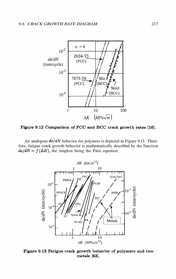
An analogous behavior for polymers is depicted in Figure 9.13. There-fore, fatigue crack growth behavior is mathematically described by the function
the simplest being the Paris equation.
9.6. CRACK GROWTH RATE DIAGRAM 217
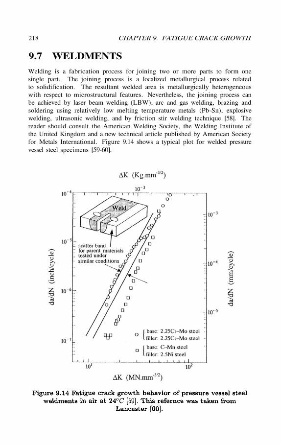
9.7 WELDMENTS
Welding is a fabrication process for joining two or more parts to form onesingle part. The joining process is a localized metallurgical process relatedto solidification. The resultant welded area is metallurgically heterogeneouswith respect to microstructural features. Nevertheless, the joining process canbe achieved by laser beam welding (LBW), arc and gas welding, brazing andsoldering using relatively low melting temperature metals (Pb-Sn), explosivewelding, ultrasonic welding, and by friction stir welding technique [58]. Thereader should consult the American Welding Society, the Welding Institute ofthe United Kingdom and a new technical article published by American Societyfor Metals International. Figure 9.14 shows a typical plot for welded pressurevessel steel specimens [59-60].
218 CHAPTER 9. FATIGUE CRACK GROWTH
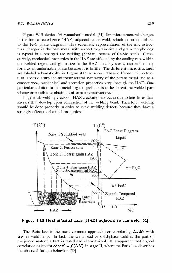
Figure 9.15 depicts Viswanathan’s model [61] for microstructural changesin the heat affected zone (HAZ) adjacent to the weld, which in turn is relatedto the Fe-C phase diagram. This schematic representation of the microstruc-tural changes in the base metal with respect to grain size and grain morphologyis typical in submerged arc welding (SMAW) process of Cr-Mo steels. Conse-quently, mechanical properties in the HAZ are affected by the cooling rate withinthe welded region and grain size in the HAZ. In alloy steels, martensite mayform as an undesirable phase because it is brittle. The different microstructuresare labeled schematically in Figure 9.15 as zones. These different microstruc-tural zones disturb the microstructural symmetry of the parent metal and as aconsequence, mechanical and corrosion properties vary through the HAZ. Oneparticular solution to this metallurgical problem is to heat treat the welded partwhenever possible to obtain a uniform microstructure.
In general, welding cracks or HAZ cracking may occur due to tensile residualstresses that develop upon contraction of the welding bead. Therefore, weldingshould be done properly in order to avoid welding defects because they have astrongly affect mechanical properties.
The Paris law is the most common approach for correlating within weldments. In fact, the weld bead or solid-phase weld is the part of
the joined materials that is tested and characterized. It is apparent that a goodcorrelation exists for in stage II, where the Paris law describesthe observed fatigue behavior [59].
9.7. WELDMENTS 219
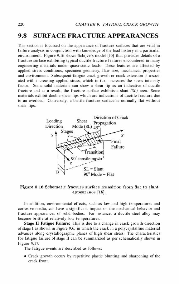
9.8 SURFACE FRACTURE APPEARANCES
This section is focussed on the appearance of fracture surfaces that are vital infailure analysis in conjunction with knowledge of the load history in a particularenvironment. Figure 9.16 shows Schijve’s model [15] that provides details of afracture surface exhibiting typical ductile fracture features encountered in manyengineering materials under quasi-static loads. These features are affected byapplied stress conditions, specimen geometry, flaw size, mechanical propertiesand environment. Subsequent fatigue crack growth or crack extension is associ-ated with increasing applied stress, which in turn increases the stress intensityfactor. Some solid materials can show a shear lip as an indicative of ductilefracture and as a result, the fracture surface exhibits a slant (SL) area. Somematerials exhibit double-shear lips which are indications of ductile fracture dueto an overload. Conversely, a brittle fracture surface is normally flat withoutshear lips.
In addition, environmental effects, such as low and high temperatures andcorrosive media, can have a significant impact on the mechanical behavior andfracture appearances of solid bodies. For instance, a ductile steel alloy maybecome brittle at relatively low temperatures.
Stage II Fatigue Failure: This is due to a change in crack growth directionof stage I as shown in Figure 9.6, in which the crack in a polycrystalline materialadvances along crystallographic planes of high shear stress. The characteristicsfor fatigue failure of stage II can be summarized as per schematically shown inFigure 9.17.
The fatigue events are described as follows:
Crack growth occurs by repetitive plastic blunting and sharpening of thecrack front.
220 CHAPTER 9. FATIGUE CRACK GROWTH
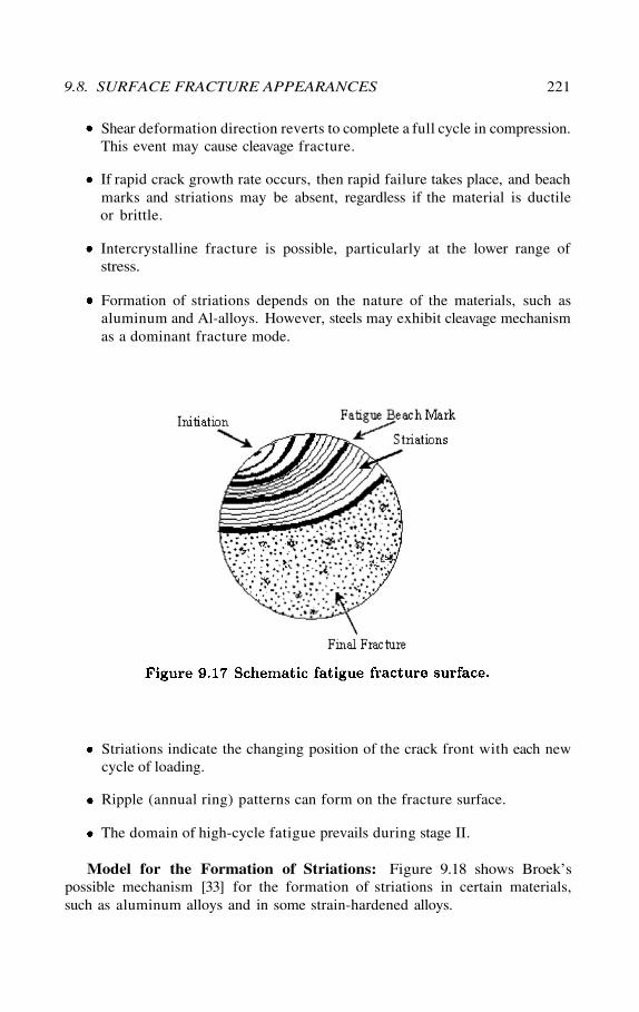
Shear deformation direction reverts to complete a full cycle in compression.This event may cause cleavage fracture.
If rapid crack growth rate occurs, then rapid failure takes place, and beachmarks and striations may be absent, regardless if the material is ductileor brittle.
Intercrystalline fracture is possible, particularly at the lower range ofstress.
Formation of striations depends on the nature of the materials, such asaluminum and Al-alloys. However, steels may exhibit cleavage mechanismas a dominant fracture mode.
Striations indicate the changing position of the crack front with each newcycle of loading.
Ripple (annual ring) patterns can form on the fracture surface.
The domain of high-cycle fatigue prevails during stage II.
Model for the Formation of Striations: Figure 9.18 shows Broek’spossible mechanism [33] for the formation of striations in certain materials,such as aluminum alloys and in some strain-hardened alloys.
9.8. SURFACE FRACTURE APPEARANCES 221
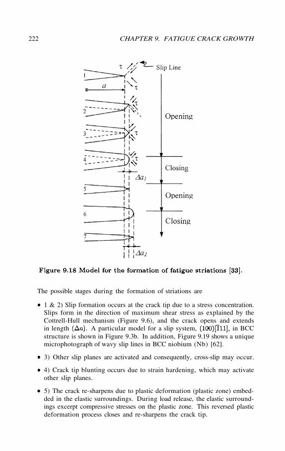
The possible stages during the formation of striations are
1 & 2) Slip formation occurs at the crack tip due to a stress concentration.Slips form in the direction of maximum shear stress as explained by theCottrell-Hull mechanism (Figure 9.6), and the crack opens and extendsin length A particular model for a slip system, in BCCstructure is shown in Figure 9.3b. In addition, Figure 9.19 shows a uniquemicrophotograph of wavy slip lines in BCC niobium (Nb) [62].
3) Other slip planes are activated and consequently, cross-slip may occur.
4) Crack tip blunting occurs due to strain hardening, which may activateother slip planes.
5) The crack re-sharpens due to plastic deformation (plastic zone) embed-ded in the elastic surroundings. During load release, the elastic surround-ings excerpt compressive stresses on the plastic zone. This reversed plasticdeformation process closes and re-sharpens the crack tip.
222 CHAPTER 9. FATIGUE CRACK GROWTH
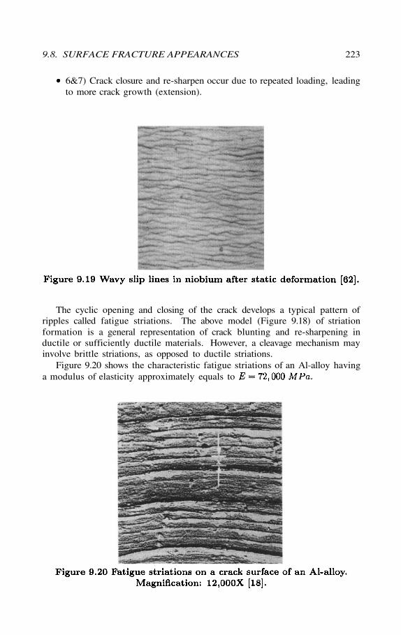
6&7) Crack closure and re-sharpen occur due to repeated loading, leadingto more crack growth (extension).
The cyclic opening and closing of the crack develops a typical pattern ofripples called fatigue striations. The above model (Figure 9.18) of striationformation is a general representation of crack blunting and re-sharpening inductile or sufficiently ductile materials. However, a cleavage mechanism mayinvolve brittle striations, as opposed to ductile striations.
Figure 9.20 shows the characteristic fatigue striations of an Al-alloy havinga modulus of elasticity approximately equals to
9.8. SURFACE FRACTURE APPEARANCES 223
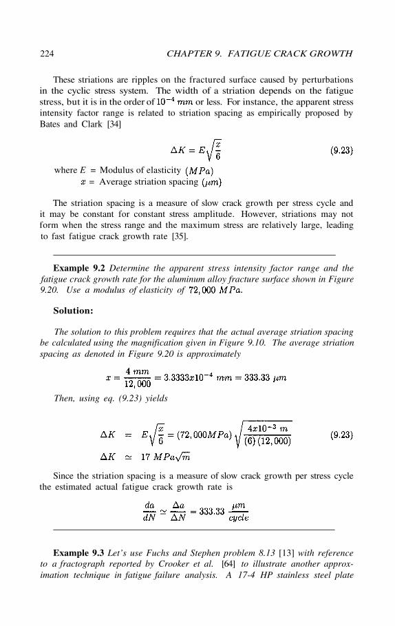
These striations are ripples on the fractured surface caused by perturbationsin the cyclic stress system. The width of a striation depends on the fatiguestress, but it is in the order of or less. For instance, the apparent stressintensity factor range is related to striation spacing as empirically proposed byBates and Clark [34]
The striation spacing is a measure of slow crack growth per stress cycle andit may be constant for constant stress amplitude. However, striations may notform when the stress range and the maximum stress are relatively large, leadingto fast fatigue crack growth rate [35].
Example 9.2 Determine the apparent stress intensity factor range and thefatigue crack growth rate for the aluminum alloy fracture surface shown in Figure9.20. Use a modulus of elasticity of
Solution:
The solution to this problem requires that the actual average striation spacingbe calculated using the magnification given in Figure 9.10. The average striationspacing as denoted in Figure 9.20 is approximately
Then, using eq. (9.23) yields
Since the striation spacing is a measure of slow crack growth per stress cyclethe estimated actual fatigue crack growth rate is
Example 9.3 Let’s use Fuchs and Stephen problem 8.13 [13] with referenceto a fractograph reported by Crooker et al. [64] to illustrate another approx-imation technique in fatigue failure analysis. A 17-4 HP stainless steel plate
224 CHAPTER 9. FATIGUE CRACK GROWTH
where E = Modulus of elasticity= Average striation spacing
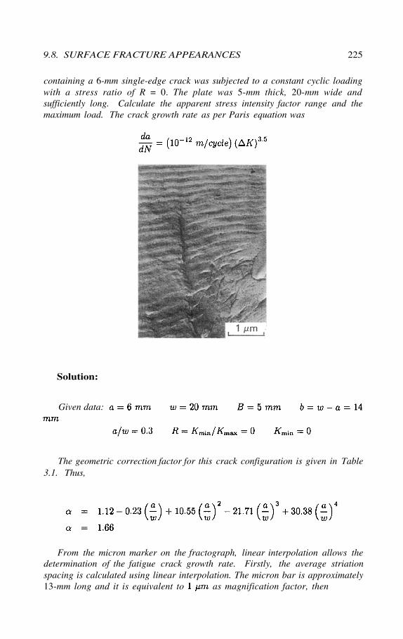
containing a 6-mm single-edge crack was subjected to a constant cyclic loadingwith a stress ratio of R = 0. The plate was 5-mm thick, 20-mm wide andsufficiently long. Calculate the apparent stress intensity factor range and themaximum load. The crack growth rate as per Paris equation was
Solution:
The geometric correction factor for this crack configuration is given in Table3.1. Thus,
From the micron marker on the fractograph, linear interpolation allows thedetermination of the fatigue crack growth rate. Firstly, the average striationspacing is calculated using linear interpolation. The micron bar is approximately13-mm long and it is equivalent to as magnification factor, then
9.8. SURFACE FRACTURE APPEARANCES 225
Given data:
For one cycle, the average striation spacing represents the crack grown percycle. Thus,
Using Paris equation yields
For comparison purposes, eq. (9.23) along with gives
which is approximately 6% lower than the previous result. Therefore, bothmethods can yield reasonable results.
Secondly, taking as the average value one can calcu-late the maximum load as follows:
226 CHAPTER 9. FATIGUE CRACK GROWTH
9.9 MIXED-MODE LOADING
The slow fatigue crack growth in elastic solids has been inves-tigated under mixed-mode interactions [36-37] and biaxial cyclic loading [36-40].A remarkable observation is that decreases as the stress ratio R increasesas in the case of mode I loading depicted in Figure 9.10. However, if the startingcrack size is large and the biaxial stress level is low, is independent of
[38].In conducting mixed-mode fatigue studies, a defined effective stress intensity
factor may be used in the Paris law for brittle [36-40] or ductile [41-44]materials. Effectively, the definition of depends on the mathematicaltechnique and theoretical background one uses. Nevertheless, the Paris law[16-17] takes the general and empirical form
For a mixed-mode I and II interaction, eq. (8.17) and (8.18) may be used todefined the effective stress intensity factor range as
For pure mode I at fracture, (similar argument was presentedin Chapter 8) for R = 0 and eqs. (9.25) and (9.26) become
Combining eqs. (8.15), (8.16), (9.27) and (9.28) yields a expression similarto eq. (8.18)
where
An example can make the above analytical procedure clearly usable for solv-ing mixed-mode problems under cyclic stress systems.
9.9. MIXED-MODE LOADING 227
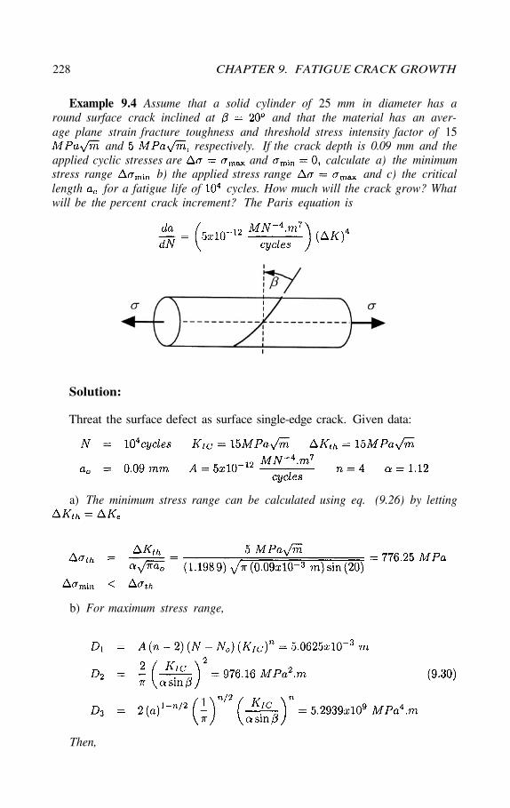
Example 9.4 Assume that a solid cylinder of 25 mm in diameter has around surface crack inclined at and that the material has an aver-age plane strain fracture toughness and threshold stress intensity factor of 15
and respectively. If the crack depth is 0.09 mm and theapplied cyclic stresses are and calculate a) the minimumstress range b) the applied stress range and c) the criticallength for a fatigue life of cycles. How much will the crack grow? Whatwill be the percent crack increment? The Paris equation is
Solution:
Threat the surface defect as surface single-edge crack. Given data:
a) The minimum stress range can be calculated using eq. (9.26) by letting
b) For maximum stress range,
228 CHAPTER 9. FATIGUE CRACK GROWTH
Then,
c) From eq. (9.28), the critical crack size is
Therefore, the crack grew which represents 6.33% crackincrement.
9.10 GROWTH RATE MEASUREMENTS
In general, for small increments of the crack length in the order of orless, the following procedure gives acceptable results. That is, the fatigue crackgrowth rate can be approximated by
Then, compute the average crack length and the specimen geometry correc-tion factor, respectively, as
and since the initial crack length exists. TheAmerican Society for Testing Materials (ASTM) E647 Standard Test Methodis widely used for measuring the crack length and the elapsed fatigue cycles atconstant loading stress amplitude and frequency. This method deals with theprocedure for determining low and high steady-state fatigue crack growth rates.This particular test method does not restrict specimen geometry and specimenthickness as long as buckling is precluded and the specimen ligament is largeenough.
9.10. GROWTH RATE MEASUREMENTS 229
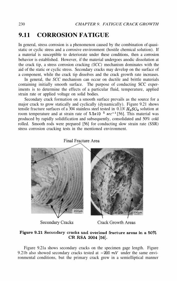
9.11 CORROSION FATIGUE
In general, stress corrosion is a phenomenon caused by the combination of quasi-static or cyclic stress and a corrosive environment (hostile chemical solution). Ifa material is susceptible to deteriorate under these conditions, then a corrosionbehavior is established. However, if the material undergoes anodic dissolution atthe crack tip, a stress corrosion cracking (SCC) mechanism dominates with theaid of the static or cyclic stress. Secondary cracks may develop on the surface ofa component, while the crack tip dissolves and the crack growth rate increases.
In general, the SCC mechanism can occur on ductile and brittle materialscontaining initially smooth surface. The purpose of conducting SCC exper-iments is to determine the effects of a particular fluid, temperature, appliedstrain rate or applied voltage on solid bodies.
Secondary crack formation on a smooth surface prevails as the source for amajor crack to grow statically and cyclically (dynamically). Figure 9.21 showstensile fracture surfaces of a 304 stainless steel tested in 0.1N solution atroom temperature and at strain rate of [56]. This material wasproduced by rapidly solidification and subsequently, consolidated and 50% coldrolled. Smooth rods were prepared [56] for conducting slow strain rate (SSR)stress corrosion cracking tests in the mentioned environment.
Figure 9.21a shows secondary cracks on the specimen gage length. Figure9.21b also showed secondary cracks tested at under the same envi-ronmental conditions, but the primary crack grew in a semielliptical manner
230 CHAPTER 9. FATIGUE CRACK GROWTH
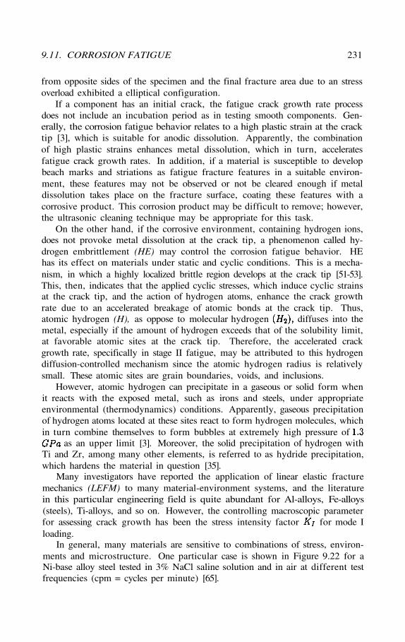
from opposite sides of the specimen and the final fracture area due to an stressoverload exhibited a elliptical configuration.
If a component has an initial crack, the fatigue crack growth rate processdoes not include an incubation period as in testing smooth components. Gen-erally, the corrosion fatigue behavior relates to a high plastic strain at the cracktip [3], which is suitable for anodic dissolution. Apparently, the combinationof high plastic strains enhances metal dissolution, which in turn, acceleratesfatigue crack growth rates. In addition, if a material is susceptible to developbeach marks and striations as fatigue fracture features in a suitable environ-ment, these features may not be observed or not be cleared enough if metaldissolution takes place on the fracture surface, coating these features with acorrosive product. This corrosion product may be difficult to remove; however,the ultrasonic cleaning technique may be appropriate for this task.
On the other hand, if the corrosive environment, containing hydrogen ions,does not provoke metal dissolution at the crack tip, a phenomenon called hy-drogen embrittlement (HE) may control the corrosion fatigue behavior. HEhas its effect on materials under static and cyclic conditions. This is a mecha-nism, in which a highly localized brittle region develops at the crack tip [51-53].This, then, indicates that the applied cyclic stresses, which induce cyclic strainsat the crack tip, and the action of hydrogen atoms, enhance the crack growthrate due to an accelerated breakage of atomic bonds at the crack tip. Thus,atomic hydrogen (H), as oppose to molecular hydrogen diffuses into themetal, especially if the amount of hydrogen exceeds that of the solubility limit,at favorable atomic sites at the crack tip. Therefore, the accelerated crackgrowth rate, specifically in stage II fatigue, may be attributed to this hydrogendiffusion-controlled mechanism since the atomic hydrogen radius is relativelysmall. These atomic sites are grain boundaries, voids, and inclusions.
However, atomic hydrogen can precipitate in a gaseous or solid form whenit reacts with the exposed metal, such as irons and steels, under appropriateenvironmental (thermodynamics) conditions. Apparently, gaseous precipitationof hydrogen atoms located at these sites react to form hydrogen molecules, whichin turn combine themselves to form bubbles at extremely high pressure of
as an upper limit [3]. Moreover, the solid precipitation of hydrogen withTi and Zr, among many other elements, is referred to as hydride precipitation,which hardens the material in question [35].
Many investigators have reported the application of linear elastic fracturemechanics (LEFM) to many material-environment systems, and the literaturein this particular engineering field is quite abundant for Al-alloys, Fe-alloys(steels), Ti-alloys, and so on. However, the controlling macroscopic parameterfor assessing crack growth has been the stress intensity factor for mode Iloading.
In general, many materials are sensitive to combinations of stress, environ-ments and microstructure. One particular case is shown in Figure 9.22 for aNi-base alloy steel tested in 3% NaCl saline solution and in air at different testfrequencies (cpm = cycles per minute) [65].
9.11. CORROSION FATIGUE 231
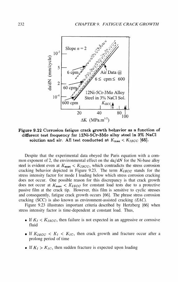
Despite that the experimental data obeyed the Paris equation with a com-mon exponent of 2, the environmental effect on the for the Ni-base alloysteel is evident even at which contradicts the stress corrosioncracking behavior depicted in Figure 9.23. The term stands for thestress intensity factor for mode I loading below which stress corrosion crackingdoes not occur. One possible reason for this discrepancy is that crack growthdoes not occur at for constant load tests due to a protectivepassive film at the crack tip. However, this film is sensitive to cyclic stressesand consequently, fatigue crack growth occurs [66]. The phrase stress corrosioncracking (SCC) is also known as environment-assisted cracking (EAC).
Figure 9.23 illustrates important criteria described by Hertzberg [66] whenstress intensity factor is time-dependent at constant load. Thus,
If then failure is not expected in an aggressive or corrosivefluid
If then crack growth and fracture occur after aprolong period of time
If then sudden fracture is expected upon loading
232 CHAPTER 9. FATIGUE CRACK GROWTH
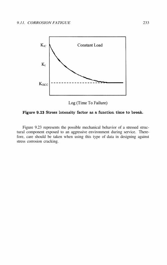
Figure 9.23 represents the possible mechanical behavior of a stressed struc-tural component exposed to an aggressive environment during service. There-fore, care should be taken when using this type of data in designing againststress corrosion cracking.
9.11. CORROSION FATIGUE 233
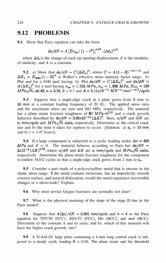
9.12 PROBLEMS
9.1 Show that Paris equation can take the form
where is the change of crack tip opening displacement, E is the modulusof elasticity, and A is a constant.
9.2 a) Show that where andis Walker’s effective stress intensity factor range. b)
Plot and for a 4340 steel having. b) Plot andfor a steel having
R = 0.7 and
9.3 Suppose that a single-edge crack in a plate grows from toat a constant loading frequency of 20 Hz. The applied stress ratio
and the maximum stress are zero and 403 MPa, respectively. The materialhas a plane strain fracture toughness of and a crack growthbehavior described by Here, and arein and respectively. Determine a) the critical cracksize and b) the time it takes for rupture to occur. [Solution: a)and b) t = 1.47 hours].
9.4 If a large component is subjected to a cyclic loading underand R = 0. The material behaves according to Paris law
where and are in andrespectively. Determine the plane-strain fracture toughness for the componentto endure 54,532 cycles so that a single-edge crack grows from 2 mm to
9.5 Consider a part made of a polycrystalline metal that is stresses in theelastic stress range. If the metal contains inclusions, has an imperfectly smoothexterior surface, and natural dislocation, would the metal experience irreversiblechanges in a micro-scale? Explain.
9.6 Why most service fatigue fractures are normally not clear?
9.7 What is the physical meaning of the slope of the stage II line in theParis model?
9.8 Suppose that and in the Parisequation for 7075-T6 (FCC), 2024-T3 (FCC), Mo (BCC), and steel (BCC).Determine a) the constant A and its units, and b), which of this material willhave the higher crack growth, rate?
9.9 A Ti-6Al-4V large plate containing a 4-mm long central crack is sub-jected to a steady cyclic loading R = 0.10. The plane strain and the threshold
234 CHAPTER 9. FATIGUE CRACK GROWTH
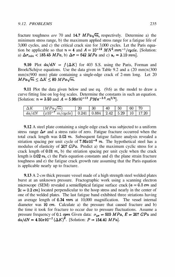
fracture toughness are 70 and respectively. Determine a) theminimum stress range, b) the maximum applied stress range for a fatigue life of3,000 cycles, and c) the critical crack size for 3,000 cycles. Let the Paris equa-tion be applicable so that and [Solution:a) b) and c)
9.10 Plot for 403 S.S. using the Paris, Forman andBroek/Schijve equations. Use the data given in Table 9.2 and a (20 mm)x(300mm)x(900 mm) plate containing a single-edge crack of 2-mm long. Let 20
9.11 Plot the data given below and use eq. (9.6) as the model to draw acurve fitting line on log-log scales. Determine the constants in such an equation.[Solution: and
9.12 A steel plate containing a single edge crack was subjected to a uniformstress range and a stress ratio of zero. Fatigue fracture occurred when thetotal crack length was Subsequent fatigue failure analysis revealed astriation spacing per unit cycle of The hypothetical steel has amodulus of elasticity of Predict a) the maximum cyclic stress for acrack length of b) the striation spacing per unit cycle when the cracklength is c) the Paris equation constants and d) the plane strain fracturetoughness and e) the fatigue crack growth rate assuming that the Paris equationis applicable nearly up to fracture.
9.13 A 2-cm thick pressure vessel made of a high strength steel welded platesburst at an unknown pressure. Fractographic work using a scanning electronmicroscope (SEM) revealed a semielliptical fatigue surface crack and
located perpendicular to the hoop stress and nearly in the center ofone of the welded plates. The last fatigue band exhibited three striations havingan average length of at 10,000 magnification. The vessel internaldiameter was Calculate a) the pressure that caused fracture and b)the time it took for fracture to occur due to pressure fluctuations. Assume apressure frequency of Given data: and
[Solution:
9.12. PROBLEMS 235
9.13 REFERENCES
[1] J.A. Collins, “Failure of Materials in Mechanical Design: Analysis, Pre-diction, Prevention,” Second Edition, John Wiley & Sons, New York (1993)181
[2] W.A. Wood. Bulletin Inst. Of Metals, Vol. 3 (1955)[3] D.K. Felbeck and A.G. Atkins, “Strength and Fracture of Engineering
Solids,” Second Edition, Prentice Hall, Inc., Upper Saddle River, NJ, (1996)430-443
[4] G.E. Dieter, “Mechanical Metallurgy,” McGraw-Hill, Inc., (1986) 178[5] K. Hellan, “Introduction to Fracture Mechanics,” McGraw-Hill Book
company, New York, (1984)[6] P.C. Paris and F. Erdogan, “A Critical Analysis of Crack Propagation
Laws,” J. Basis Engineering, Trans. ASME, Vol. 85(1963) 528-534[7] R.G. Forman at el., Trans. ASME 89 (1967) 459-464[8] D. Broek and J. Schijve, National Aerospace Laboratory, Amsterdam,
Report NLR-TR-M-2111, (1963)[9] F. Endorgan, “Crack Propagation Theories,” NASA-CR-901, (1967)[10] E.K. Walker, ASTM STP 462 (1970) 1-14[11] A. Hartman and J. Schijve, Eng. Fracture Mechanics, 1(1970)[12] R.O. Ritchie, “Near-Threshold Fatigue Crack Propagation,” Inter. Met-
als Reviews, Vol. 24(5) (1979)[13] H.O. Fuchs and R.I. Stephens, “Metal Fatigue in Engineering,” John
Wiley & Sons, New York, 1980[14] J.M. Barsom and S.T. Rolfe, “Fracture and Fatigue in Structure: Ap-
plication of fracture Mechanics,” Third edition, American Society for Testingand Materials, Philadelphia, PA, (1999).
[15] J. Schijve, Fatigue Thresholds, Vol. 2 EMAS Ltd., West Midlands,England, (1982)
[16] P.C. Paris, “Fracture Mechanics Approach to Fatigue.” Fatigue-AnInterdisciplinary Approach, J.J. Burke at el., Editor. Proc. 10th SagamoreArmy Matl. Research Conf., Syracuse University Press, Syracuse, NY (1964)
[17] P.C. Paris et al., ASTM STP 513 (1972) 141-176[18] E.J. Imhoff and J.M. Barsoum, ASTM STP 536 (1973)[19] M.D. Speidel, NACE Stress Corrosion Cracking and Hydrogen Embrit-
tlement of Iron Base Alloys, Vilieux, France, (June 1973)[20] W.W. Gerberich et al., Corrosion Fatigue, NACE-2, Houston, (1972)[21] A.J. McEvily and J.L. Gonzalez, Metallurgical Trans. A, Vol. 23A
(Aug. 1992)[22] P. Shahinian et al., ASTM STP 520 (1973)[23] W.A. Logsdon, Eng. Fracture Mechanics, Vol. 7(1) (March 1975)[24] L. Abrego and J.A. Begley, in International Corrosion Forum, Palmer
House, Chicago, March 3-7 (1980)[25] W.J. Mills, J. Eng. Materials and Technology, Trans. ASME Vol. 100(2)
(1978)
236 CHAPTER 9. FATIGUE CRACK GROWTH
[26] L.A. James, Report HEDL-TME-75-82, Westinghouse Hanford Co.,Richland, WA, (January 1976)
[27] Report MDC-A0913, Phase B Test Program, McDonnell Aircraft Co.,McDonnell Douglas Corp., St. Louis, (May 1971)
[28] J.C. Zola, Case Studies in Fracture Mechanics, edited by T.P. Rich andD.J. Cartwright, AMMRC MS 77-5 Army Materials and Mechanics ResearchCenter, Watertown, MA (1996)
[29] R.L. Tobler, Cryogenics, Vol. 16(11) (1976)[30] W.J. Mills and L.A. James, ASME Publication 7-WA/PUP-3, (1979)[31] R.W. Bush et al., “Fracture Mechanics Characteristics of High Strength
Aluminum Alloy Forging,” ALCOA Forged Products, Report Q-395 (1993)[32] H.M. Westergaard, “Bearing Pressures and Cracks,” J. Appl. Mech.,
G1 (1939) A49 - A53[33] D. Broek, “Elementary Engineering Fracture Mechanics,” Fourth edi-
tion, Kluwer Academic Publisher, Boston, (1986)[34] R.C. Bates and W.G. Clark, Jr., Trans. Quarterly ASM 62(2) (1969)[35] T.H. Courtney, “Mechanical Behavior of Materials,” McGraw-Hill Pub-
lishing Co., N.Y. (1990)[36] K.J. Miller and A.P. Kfouri, Inter. J. Fracture, Vol. 10(3) (1974)[37] N.J. Adams, Eng. Fracture Mechanics, Vol. 5 (1973)[38] H. Kitagawa et al., ASTM STP 853, (1985)[39] T. Hishide et al., Fatigue Eng. And Materials Structure, Vol. 4, No. 4,
(1981)[40] A. Liu et al., ASTM STP 677, (1979)[41] W. Elber, ASTM STP 486 (1971) 230[42] F. Erdogan and G.C. Sih, J. Basic Eng., 85 (1963) 519[43] H. Qingzhi, Fatigue Eng. Mat. Structure, 7 (1984) 41[44] W. Wei and H. Qingzhi, Proc. Far East Fracture Group Workshop,
Tokyo Institute of Technology, Japan, Nov. 28-30 (1988) 193.[45] E.A. Loria, Mat. Sci. Eng., A254 (1998) 63.[46] F.Y.C. Mercer and W.D. Soboyego, Metall. Mat. Trans. A, Vol. 29A
(1998) 2361[47] A. Tonneau et al., Mat. Sci. Eng, A256 (1998) 256.[48] M.A. Daeubler et al., Metall. Tran A, Vol. 21 A (1990) 925.[49] J.M. Barsom, Ph.D. Dissertation, University of Pittsburgh, PA (1969)[50] J.M. Barsom, ASTM STP 486, (1971) 1-15[51] H. Vehoff and H.K. Klameth, “Hydrogen Embrittlement and Trapping
at Crack Tips in Ni-Single Crystals”, Perspect in Hydrogen in Met., (1986)661-668
[52] J.S. Wang, “Hydrogen Induced Embrittlement and the Effect of theMobility of Hydrogen Atoms,” Proc. of the 1994 5th Inter. Conf. on the Effectof Hydrogen on the Behavior of Materials, , Mora, WY, USA, (Sept. 11-14,1994) 61-75
[53] R.P. Gangloff, “Crack Tip Modeling of Hydrogen Environment Em-brittlement: Application to Fracture Mechanics Life Prediction,” Materials &Engineering A, Vol. A103, 1 (Aug. 1988) 157-166
9.13. REFERENCES 237
[54] N. Perez, “Strengthening Mechanism of Alloy,” Journal of MechanicalBehavior of Materials, March (1999)
[55] N. Perez and T.A. Place, “X-Ray Diffraction of a Heat Treated RapidlySolidified Alloy”, Journal of Materials Science Letters, 9 (1990) 940-942.
[56] N Perez, Ph.D. Dissertation, University of Idaho, USA,(1989)[57] A. Riddick, “Testing for Fatigue Crack Growth,” Advance Materials &
Processing, (October 2003) 53-55[58] R.S. Mishra, “Friction Stir Processing Technologies,” Advance Materials
& Processing, (October 2003) 43-46[59] L.A. James, Elding Journal, 56 (19777) 386-391[60] J.F. Lancaster, “Metallurgy of Welding,” Fifth edition, Chapman &
Hall, New York, (1993) 356[61] R. Viswanathan, “Damage Mechanisms and Life Assessment of High-
Temperature Components,” ASM international, (1989)[62] A. Kelly and G.W. Groves, “Crystallography and Crystal Defects,”
Addisson-Wesley Publishing Company,Reading, Massachusetts, (1970) 212[63] J.A. Manson et al., Advances in Fracture Research, D. Francois et al.
editors, Pergamon Press, Oxford, (1980)[64] T.W. Crooker, D.F. Hasson and G.R. Yoder, “Micromechanistic Inter-
pretation of Cyclic Crack Growth Behavior in 17-4 PH Stainless Steel,” Frac-tography: Microscopic Cracking Processes, ASTM STP 600, (1976) 205
[65] E.J. Imhof and J.M. Barsom, ASTM STP 536, (1973) 182[66] R.W. Hertz berg, “Deformation and Fracture Mechanics of Engineering
Materials”, third edition, John Wiley & Sons, New York, (1989)
238 CHAPTER 9. FATIGUE CRACK GROWTH
Chapter 10
FRACTURE TOUGHNESSCORRELATIONS
10.1 INTRODUCTION
This chapter is devoted to a brief review of fracture toughness of crack-free andnotched specimens. Fracture toughness can be defined as the strain energy ab-sorbed by a material prior to fracture. Thus, this energy is defined as the strainenergy density in a tension test, the intensity of the stresses ahead of acrack tip, the strain-energy release rate also known as the crack driving force
or for crack growth or the dynamic strain energy (U) for conventionaland instrumented Charpy impact tests. Some useful empirical correlations fordetermining the plane strain fracture toughness from Vickers microhard-ness measurements and impact tests are included.
Furthermore, impact testing and microhardness measurement techniques arewidely used in materials evaluation since they are simple and cost effective.Thus, fracture toughness correlations have evolved indicating the usefulnessof the impact and indentation techniques when proper precautions are takenin conducting experiments. For instance, the dynamic behavior of the Charpyimpact test can be understood by modeling the striker and specimen as a spring-mass system.
10.2 CRACK-FREE BODIES UNDER TENSION
In general, the mechanical behavior of a material under a stress-loading modedepends on the microstructure, strain rate, and environment. The behavior ofan initially crack-free material is characterized by one of the typical stress-straincurves shown in Figure 10.1. Typical tension properties, such as yield strength,tensile strength, ductility, and the modulus of elasticity are obtained from thesecurves. The strength refers to a property and stress is a parameter related to an
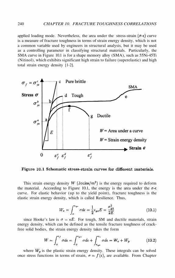
applied loading mode. Nevertheless, the area under the stress-strain curveis a measure of fracture toughness in terms of strain energy density, which is nota common variable used by engineers in structural analysis, but it may be usedas a controlling parameter in classifying structural materials. Particularly, theSMA curve in Figure 10.1 is for a shape memory alloy (SMA), such as 55Ni-45Ti(Nitinol), which exhibits significant high strain to failure (superelastic) and hightotal strain energy density [1-2].
This strain energy density is the energy required to deformthe material. According to Figure 10.1, the energy is the area under thecurve. For elastic behavior (up to the yield point), fracture toughness is theelastic strain energy density, which is called Resilience. Thus,
since Hooke’s law is For tough, SM and ductile materials, strainenergy density, which can be defined as the tensile fracture toughness of crack-free solid bodies, the strain energy density takes the form
where is the plastic strain energy density. These integrals can be solvedonce stress functions in terms of strain, are available. From Chapter
240 CHAPTER 10. FRACTURE TOUGHNESS CORRELATIONS
7, the most common plastic stress functions are known as Ramberg-Osgood andHollomon equations, respectively
These equations are valid from the yield strength to the maximum or ul-timate tensile strength stress on the stress-strain curves. In other words, thelimit points are and
For a strain hardenable material, the Ramberg-Osgood or Hollomon equationmay be used as an effective stress expression so that the integral can easily besolved. Substituting eqs. (10.3) and (10.4) into (10.2) yields general solutions
Using proper integral limits, these equations become, respectively
An ideal tough material must exhibit high strength and ductility. Despiteductile materials are considered tough; they have low strength and high ductility.However, if a notched tensile specimen, made of a ductile material, is loadedin tension, the plastic flow is shifted upwards since a triaxial state of stress isdeveloped at the root of the notch. This is a constraint against plastic flow, butit enhances the magnitude of the elastic stresses at the notch root [3].
In summary, the yield strength and the fracture toughness in terms of totalstrain energy density of crack-free materials can be compared using the inequal-ities shown below
This analogy implies that fracture toughness decreases with increasing strengthand decreasing strain to failure.
10.2. CRACK-FREE BODIES UNDER TENSION 241
10.3 GRAIN SIZE REFINEMENT
The grain size refinement technique, which has been successfully applied to someBody-Centered Cubic (BCC) steels containing molybdenum (Mo), vanadium(V) , titanium and aluminum is one approach for enhancing bothyield strength and fracture toughness. These alloying elements react in the solid-solution state to form either particles or cause microstructural changes that areaccountable for pinning grain boundaries, and therefore, austenite grain growthis retained on cooling.
In addition, these elements can restrain the coarsening of carbide particles,which in turn pin dislocation motion on deformation by external stresses. Theexact microstructural and phase transformation mechanism evolved in addingthese elements to carbon steels is a particular metallurgical topic that canbe found elsewhere [4]. Subsequently, the controlling property, such as yieldstrength or fracture toughness, is limited to 1) the strength if an applied exter-nal load exists, 2) the fracture toughness if absorption of strain energy occursprior to fracture, and 3) the ductility if metal shaping or forming is required.
The addition of small amounts of alloying elements, such as V,and the like, to carbon steels enhances the strength and fracture toughnessof these important engineering materials. As mentioned in Chapter 2, this isreferred to as the grain-size refinement technique. Thus, the yield strength,fracture strength, and fracture toughness can be correlated with grain size andcorrelations can be accomplished experimentally [5-7] and empirically by usingthe Orowan [8] and the Hahn-Rosenfield [9] plastic constraint factor at thecrack tip, respectively, defined by
The most common relationships for correlating the yield and fracture strengthswith grain size is known as the Hall-Petch type equation defined as
where = Friction stress due to particle, dislocations, grain boundary andthe like
= Stress constant= Dislocation locking term= Constant
= Grain size
where for strain hardening mild steels [9].
242 CHAPTER 10. FRACTURE TOUGHNESS CORRELATIONS
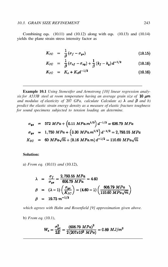
Combining eqs. (10.11) and (10.12) along with eqs. (10.13) and (10.14)yields the plane strain stress intensity factor as
Example 10.1 Using Stonesifer and Armstrong [10] linear regression analy-sis for A533B steel at room temperature having an average grain size ofand modulus of elasticity of 207 GPa, calculate Calculate a) and and b)predict the elastic strain energy density as a measure of elastic fracture toughnessfor sound specimens subjected to tension loading an determine.
Solution:
a) From eq. (10.11) and (10.12),
which agrees with Hahn and Rosenfield [9] approximation given above.
b) From eq. (10.1),
10.3. GRAIN SIZE REFINEMENT 243
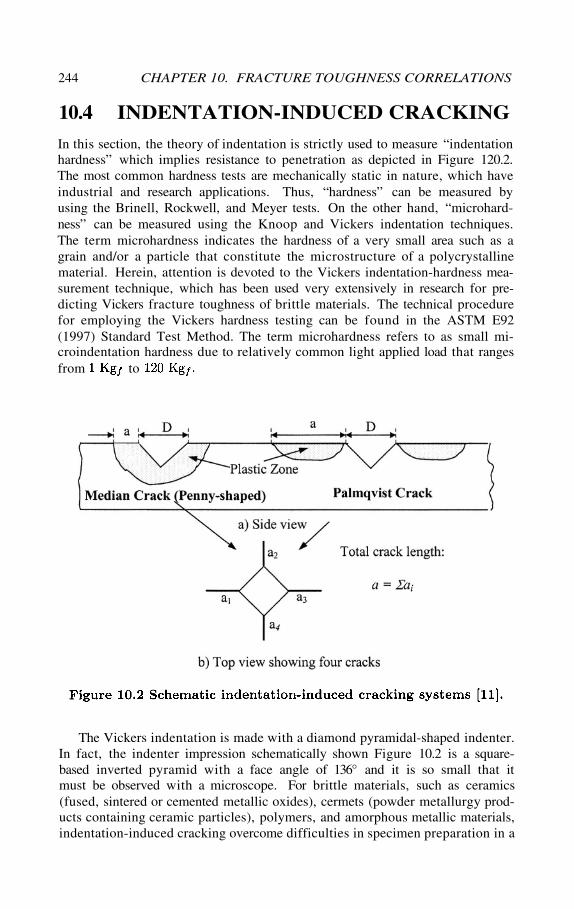
10.4 INDENTATION-INDUCED CRACKING
In this section, the theory of indentation is strictly used to measure “indentationhardness” which implies resistance to penetration as depicted in Figure 120.2.The most common hardness tests are mechanically static in nature, which haveindustrial and research applications. Thus, “hardness” can be measured byusing the Brinell, Rockwell, and Meyer tests. On the other hand, “microhard-ness” can be measured using the Knoop and Vickers indentation techniques.The term microhardness indicates the hardness of a very small area such as agrain and/or a particle that constitute the microstructure of a polycrystallinematerial. Herein, attention is devoted to the Vickers indentation-hardness mea-surement technique, which has been used very extensively in research for pre-dicting Vickers fracture toughness of brittle materials. The technical procedurefor employing the Vickers hardness testing can be found in the ASTM E92(1997) Standard Test Method. The term microhardness refers to as small mi-croindentation hardness due to relatively common light applied load that rangesfrom to
The Vickers indentation is made with a diamond pyramidal-shaped indenter.In fact, the indenter impression schematically shown Figure 10.2 is a square-based inverted pyramid with a face angle of 136° and it is so small that itmust be observed with a microscope. For brittle materials, such as ceramics(fused, sintered or cemented metallic oxides), cermets (powder metallurgy prod-ucts containing ceramic particles), polymers, and amorphous metallic materials,indentation-induced cracking overcome difficulties in specimen preparation in a
244 CHAPTER 10. FRACTURE TOUGHNESS CORRELATIONS
conventional manner as recommended by the American Society for Testing Ma-terials (ASTM) E399 for plane strain fracture toughness and for the J-integralapproach. As a result, an empirical equation may be used to determine theVickers fracture toughness.
The Vickers hardness can be calculated as follows
where P = Applied load (Kg)
D = Mean diagonal (mm)
= 136° = Face angle
The advantages of Vickers hardness measurements are 1) its simplicity, 2) itcan be applied to microstructural constituents, 3) it does not require fatigue pre-cracking, which is difficult to accomplish in brittle materials, 4) it is cost effectivesince small specimens are needed, 5) the tests are considered non-destructivein a macroscale. However, specimen preparation is a slightly time consumingprocedure since a polished surface is required so that uniform indentations aremade on a reflective flat plane, which it is must in order to obtain consistentand reproducible results.
In fact, hardness measurements are made for screening materials and char-acterizing microstructures, subsequent use is made for determining the Vickersfracture toughness, which inevitably shows some degree of inaccuracy whencompared with conventional fracture toughness. Nevertheless, this techniquehas become an excellent approach for characterizing ceramics, cermets (e.g.
WC-Co composites), and amorphous metals and their alloys.
In 1950’s, Palmquist [12] recognized that indentation-induced cracking ob-served on cermets was related to fracture toughness and he developed a proce-dure to predict fracture toughness. Vickers is the most common and suitabletest method due to four possible cracks that may emanate from the corners ofthe indenter. A typical Palmquist fracture toughness analysis requires a linearplot of total crack length vs. applied load (P); that is, Thisis shown in Figure 10.3 for an Alumina-Titanium carbide cermetThe inverse of the slope of the line is a measure of Palmquist Fracture Toughnessin terms of work done which may be taken as the strain-energy releaserate [13].
The prediction of fracture toughness for many brittle materials using em-pirical formulations can be found in the literature [14-18]. However, the mostcommon expression is the following general form
10.4. INDENTATION-INDUCED CRACKING 245
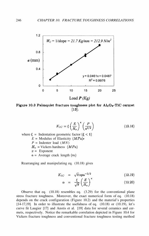
where = Indentation geometric factorE = Modulus of ElasticityP = Indenter load (MN )
= Vickers hardness= Exponent= Average crack length
Rearranging and manipulating eq. (10.18) gives
Observe that eq. (10.18) resembles eq. (3.29) for the conventional planestress fracture toughness. Moreover, the exact numerical form of eq. (10.18)depends on the crack configuration (Figure 10.2) and the material’s properties[14-17,19]. In order to illustrate the usefulness of eq. (10.18) or (10.19), let’scurve fit Laugier [17] and Anstis et al. [19] data for several ceramics and cer-mets, respectively. Notice the remarkable correlation depicted in Figure 10.4 forVickers fracture toughness and conventional fracture toughness testing method
246 CHAPTER 10. FRACTURE TOUGHNESS CORRELATIONS
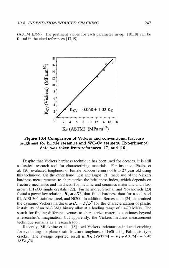
(ASTM E399). The pertinent values for each parameter in eq. (10.18) can befound in the cited references [17,19].
Despite that Vickers hardness technique has been used for decades, it is stilla classical research tool for characterizing materials. For instance, Phelps etal. [20] evaluated toughness of female baboon femurs of 6 to 27 year old usingthis technique. On the other hand, Iost and Bigot [21] made use of the Vickershardness measurements to characterize the brittleness index, which depends onfracture mechanics and hardness, for metallic and ceramics materials, and flux-grown ErFeO3 single crystals [22]. Furthermore, Sridhar and Yovanovich [23]found a power law relation, that fitted hardness data for a tool steel01, AISI 304 stainless steel, and Ni200. In addition, Berces et al. [24] determinedthe dynamic Vickers hardness as for the characterization of plasticinstability of an Al-3.3Mg binary alloy at a loading range of 1.4-70 MN/s. Thesearch for finding different avenues to characterize materials continues beyonda researcher’s imagination, but apparently, the Vickers hardness measurementtechnique remains as a research tool.
Recently, Milekhine et al. [18] used Vickers indentation-induced crackingfor evaluating the plane strain fracture toughness of FeSi using Palmquist typecracks. The average reported result is
10.4. INDENTATION-INDUCED CRACKING 247
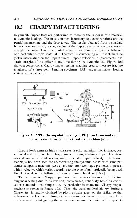
10.5 CHARPY IMPACT TESTING
In general, impact tests are performed to measure the response of a materialto dynamic loading. The most common laboratory test configurations are thependulum machine and the drop tower. The results obtained from a standardimpact tests are usually a single value of the impact energy or energy spent ona single specimen. This is of limited value in describing the dynamic behaviorof a particular sample material. Therefore, instrumenting an impact machineyields information on the impact forces, impact velocities, displacements, andstrain energies of the striker at any time during the dynamic test. Figure 10.5shows a conventional Charpy impact testing machine used to measure fracturetoughness of a three-point bending specimen (3PB) under an impact loadingsystem at low velocity.
Impact loads generate high strain rates in solid materials. For instance, con-ventional and instrumented Charpy impact testing machines impart low strainrates at low velocity when compared to ballistic impact velocity. The formertechnique has been used for characterizing the dynamic behavior of some par-ticular composite materials [25-32] and the latter technique promotes impact ata high velocity, which varies according to the type of gun projectile being used.Excellent work in the ballistic field can be found elsewhere [33-36].
The instrumented Charpy impact machine remains a key means for fracturetoughness testing due to its low cost, convenience, reliability based on certifi-cation standards, and simple use. A particular instrumented Charpy impactmachine is shown in Figure 10.6. Thus, the transient load history during aCharpy test is readily obtained by placing strain gages on the striker so thatit becomes the load cell. Using software during an impact one can record thedisplacements by integrating the acceleration versus time twice with respect to
248 CHAPTER 10. FRACTURE TOUGHNESS CORRELATIONS
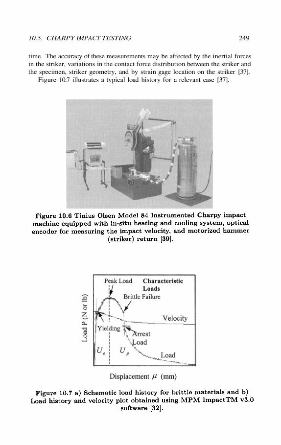
time. The accuracy of these measurements may be affected by the inertial forcesin the striker, variations in the contact force distribution between the striker andthe specimen, striker geometry, and by strain gage location on the striker [37].
Figure 10.7 illustrates a typical load history for a relevant case [37].
10.5. CHARPY IMPACT TESTING 249
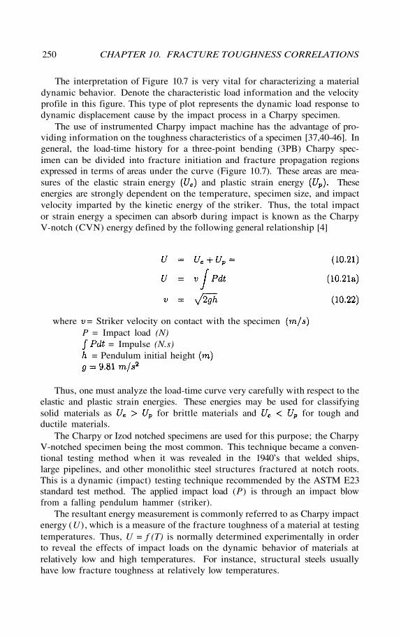
The interpretation of Figure 10.7 is very vital for characterizing a materialdynamic behavior. Denote the characteristic load information and the velocityprofile in this figure. This type of plot represents the dynamic load response todynamic displacement cause by the impact process in a Charpy specimen.
The use of instrumented Charpy impact machine has the advantage of pro-viding information on the toughness characteristics of a specimen [37,40-46]. Ingeneral, the load-time history for a three-point bending (3PB) Charpy spec-imen can be divided into fracture initiation and fracture propagation regionsexpressed in terms of areas under the curve (Figure 10.7). These areas are mea-sures of the elastic strain energy and plastic strain energy Theseenergies are strongly dependent on the temperature, specimen size, and impactvelocity imparted by the kinetic energy of the striker. Thus, the total impactor strain energy a specimen can absorb during impact is known as the CharpyV-notch (CVN) energy defined by the following general relationship [4]
Thus, one must analyze the load-time curve very carefully with respect to theelastic and plastic strain energies. These energies may be used for classifyingsolid materials as for brittle materials and for tough andductile materials.
The Charpy or Izod notched specimens are used for this purpose; the CharpyV-notched specimen being the most common. This technique became a conven-tional testing method when it was revealed in the 1940’s that welded ships,large pipelines, and other monolithic steel structures fractured at notch roots.This is a dynamic (impact) testing technique recommended by the ASTM E23standard test method. The applied impact load (P) is through an impact blowfrom a falling pendulum hammer (striker).
The resultant energy measurement is commonly referred to as Charpy impactenergy (U), which is a measure of the fracture toughness of a material at testingtemperatures. Thus, U = f (T) is normally determined experimentally in orderto reveal the effects of impact loads on the dynamic behavior of materials atrelatively low and high temperatures. For instance, structural steels usuallyhave low fracture toughness at relatively low temperatures.
where = Striker velocity on contact with the specimenP = Impact load (N)
= Impulse (N.s)= Pendulum initial height
250 CHAPTER 10. FRACTURE TOUGHNESS CORRELATIONS
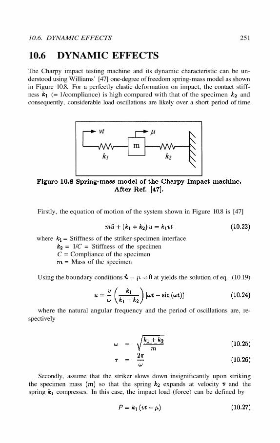
10.6 DYNAMIC EFFECTS
The Charpy impact testing machine and its dynamic characteristic can be un-derstood using Williams’ [47] one-degree of freedom spring-mass model as shownin Figure 10.8. For a perfectly elastic deformation on impact, the contact stiff-ness (= 1/compliance) is high compared with that of the specimen andconsequently, considerable load oscillations are likely over a short period of time
Firstly, the equation of motion of the system shown in Figure 10.8 is [47]
where = Stiffness of the striker-specimen interface= 1/C = Stiffness of the specimen
C = Compliance of the specimen= Mass of the specimen
Using the boundary conditions at yields the solution of eq. (10.19)
where the natural angular frequency and the period of oscillations are, re-spectively
Secondly, assume that the striker slows down insignificantly upon strikingthe specimen mass so that the spring expands at velocity and thespring compresses. In this case, the impact load (force) can be defined by
10.6. DYNAMIC EFFECTS 251
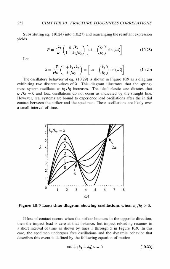
Substituting eq. (10.24) into (10.27) and rearranging the resultant expressionyields
Let
The oscillatory behavior of eq. (10.29) is shown in Figure 10.9 as a diagramexhibiting two discrete values of This diagram illustrates that the spring-mass system oscillates as increases. The ideal elastic case dictates that
and load oscillations do not occur as indicated by the straight line.However, real systems are bound to experience load oscillations after the initialcontact between the striker and the specimen. These oscillations are likely overa small interval of time.
If loss of contact occurs when the striker bounces in the opposite direction,then the impact load is zero at that instance, but impact reloading resumes ina short interval of time as shown by lines 1 through 5 in Figure 10.9. In thiscase, the specimen undergoes free oscillations and the dynamic behavior thatdescribes this event is defined by the following equation of motion
252 CHAPTER 10. FRACTURE TOUGHNESS CORRELATIONS
The loss of contact occurs when P = 0 and as a result, eq. (10.28) gives
and
Combining eqs. (10.21a) and (10.28) and integrating the resultant expressionyields the impact energy lost by the striker
This expression illustrates that the striker kinetic energy is trans-formed into strain energy U, which is absorbed by the specimen during theimpact process. However, this dynamic event exhibits an oscillation behaviorto the impact response as indicated by the cosine term in eq. (10.33). Conse-quently, bouncing generates load oscillations and gives discrete values of energyas illustrated in Figure 10.9 where all curves coincide when Thus, eq.(10.33) becomes [47]
For rigid body contact, the stiffness ratios becomes orand eq. (10.34) yields a simplified form of the impact strain energy
Analysis of theoretical and experimental data is a very important issue be-cause erroneous conclusions may be drawn. For example, plotting eq. (10.33)when and yields different dynamic behavior, while kineticenergy is converted to strain energy as the specimen bends and slows down. Theobvious significance of this observation is shown in Figure 10.10. The curvesfor coincide at This is attributed to the first load oscillationsince this behavior is also observed in Figure 10.9. Eventually, a second impactmay occur at time predicted by eq. (10.26) for further kinetic energy transfer.
10.6. DYNAMIC EFFECTS 253
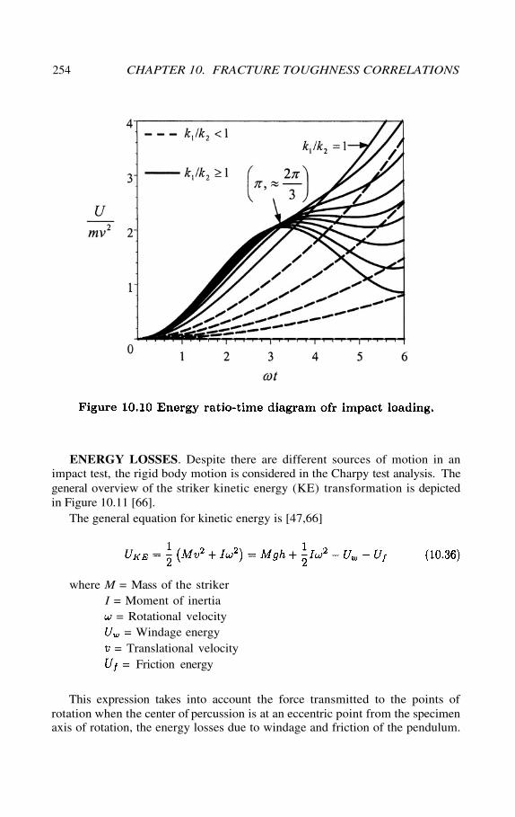
ENERGY LOSSES. Despite there are different sources of motion in animpact test, the rigid body motion is considered in the Charpy test analysis. Thegeneral overview of the striker kinetic energy (KE) transformation is depictedin Figure 10.11 [66].
The general equation for kinetic energy is [47,66]
where M = Mass of the strikerI = Moment of inertia
= Rotational velocity= Windage energy
= Translational velocity= Friction energy
This expression takes into account the force transmitted to the points ofrotation when the center of percussion is at an eccentric point from the specimenaxis of rotation, the energy losses due to windage and friction of the pendulum.
254 CHAPTER 10. FRACTURE TOUGHNESS CORRELATIONS
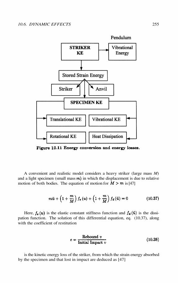
A convenient and realistic model considers a heavy striker (large mass M)and a light specimen (small mass in which the displacement is due to relativemotion of both bodies. The equation of motion for is [47]
Here, is the elastic constant stiffness function and is the dissi-pation function. The solution of this differential equation, eq. (10.37), alongwith the coefficient of restitution
is the kinetic energy loss of the striker, from which the strain energy absorbedby the specimen and that lost in impact are deduced as [47]
10.6. DYNAMIC EFFECTS 255
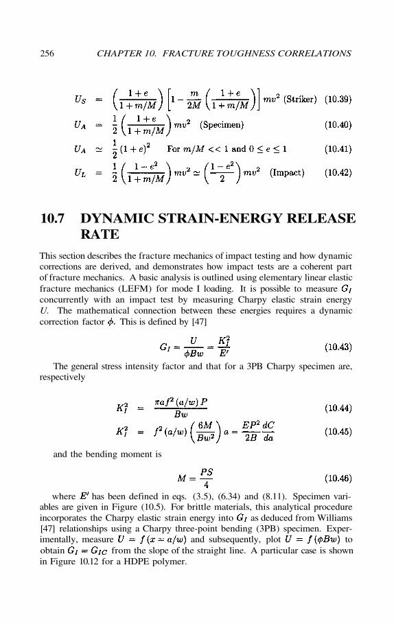
10.7 DYNAMIC STRAIN-ENERGY RELEASERATE
This section describes the fracture mechanics of impact testing and how dynamiccorrections are derived, and demonstrates how impact tests are a coherent partof fracture mechanics. A basic analysis is outlined using elementary linear elasticfracture mechanics (LEFM) for mode I loading. It is possible to measureconcurrently with an impact test by measuring Charpy elastic strain energyU. The mathematical connection between these energies requires a dynamiccorrection factor This is defined by [47]
The general stress intensity factor and that for a 3PB Charpy specimen are,respectively
and the bending moment is
where has been defined in eqs. (3.5), (6.34) and (8.11). Specimen vari-ables are given in Figure (10.5). For brittle materials, this analytical procedureincorporates the Charpy elastic strain energy into as deduced from Williams[47] relationships using a Charpy three-point bending (3PB) specimen. Exper-imentally, measure and subsequently, plot toobtain from the slope of the straight line. A particular case is shownin Figure 10.12 for a HDPE polymer.
256 CHAPTER 10. FRACTURE TOUGHNESS CORRELATIONS
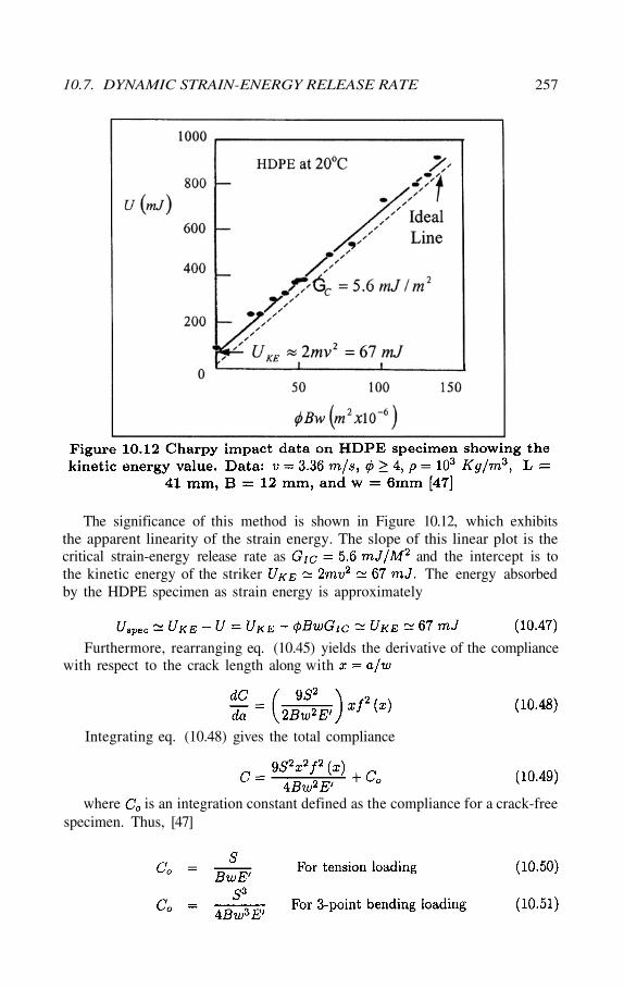
The significance of this method is shown in Figure 10.12, which exhibitsthe apparent linearity of the strain energy. The slope of this linear plot is thecritical strain-energy release rate as and the intercept is tothe kinetic energy of the striker The energy absorbedby the HDPE specimen as strain energy is approximately
Furthermore, rearranging eq. (10.45) yields the derivative of the compliancewith respect to the crack length along with
Integrating eq. (10.48) gives the total compliance
where is an integration constant defined as the compliance for a crack-freespecimen. Thus, [47]
10.7. DYNAMIC STRAIN-ENERGY RELEASE RATE 257
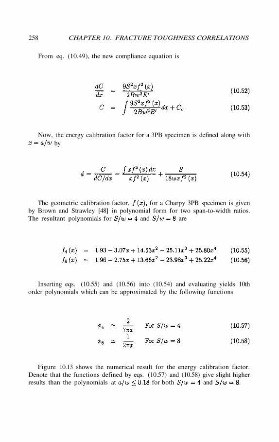
From eq. (10.49), the new compliance equation is
Now, the energy calibration factor for a 3PB specimen is defined along withby
The geometric calibration factor, for a Charpy 3PB specimen is givenby Brown and Strawley [48] in polynomial form for two span-to-width ratios.The resultant polynomials for and are
Inserting eqs. (10.55) and (10.56) into (10.54) and evaluating yields 10thorder polynomials which can be approximated by the following functions
Figure 10.13 shows the numerical result for the energy calibration factor.Denote that the functions defined by eqs. (10.57) and (10.58) give slight higherresults than the polynomials at for both and
258 CHAPTER 10. FRACTURE TOUGHNESS CORRELATIONS
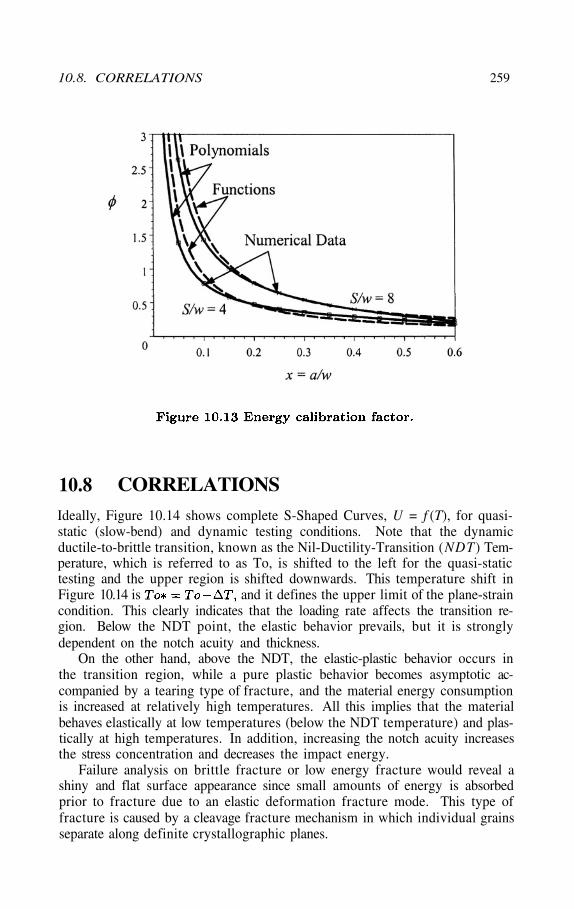
CORRELATIONS10.8Ideally, Figure 10.14 shows complete S-Shaped Curves, U = f (T), for quasi-static (slow-bend) and dynamic testing conditions. Note that the dynamicductile-to-brittle transition, known as the Nil-Ductility-Transition (NDT) Tem-perature, which is referred to as To, is shifted to the left for the quasi-statictesting and the upper region is shifted downwards. This temperature shift inFigure 10.14 is and it defines the upper limit of the plane-straincondition. This clearly indicates that the loading rate affects the transition re-gion. Below the NDT point, the elastic behavior prevails, but it is stronglydependent on the notch acuity and thickness.
On the other hand, above the NDT, the elastic-plastic behavior occurs inthe transition region, while a pure plastic behavior becomes asymptotic ac-companied by a tearing type of fracture, and the material energy consumptionis increased at relatively high temperatures. All this implies that the materialbehaves elastically at low temperatures (below the NDT temperature) and plas-tically at high temperatures. In addition, increasing the notch acuity increasesthe stress concentration and decreases the impact energy.
Failure analysis on brittle fracture or low energy fracture would reveal ashiny and flat surface appearance since small amounts of energy is absorbedprior to fracture due to an elastic deformation fracture mode. This type offracture is caused by a cleavage fracture mechanism in which individual grainsseparate along definite crystallographic planes.
10.8. CORRELATIONS 259
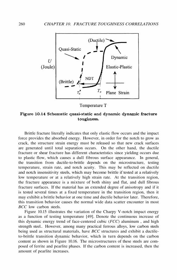
Brittle fracture literally indicates that only elastic flow occurs and the impactforce provides the absorbed energy. However, in order for the notch to grow ascrack, the structure strain energy must be released so that new crack surfacesare generated until total separation occurs. On the other hand, the ductilefracture or shear fracture has different characteristics since yielding occurs dueto plastic flow, which causes a dull fibrous surface appearance. In general,the transition from ductile-to-brittle depends on the microstructure, testingtemperature, strain rate, and notch acuity. This may be reflected on ductileand notch insensitivity steels, which may become brittle if tested at a relativelylow temperature or at a relatively high strain rate. At the transition region,the fracture appearance is a mixture of both shiny and flat, and dull fibrousfracture surfaces. If the material has an extended degree of anisotropy and if itis tested several times at a fixed temperature in the transition region, then itmay exhibit a brittle behavior at one time and ductile behavior later. Therefore,this transition behavior causes the normal wide data scatter encounter in mostBCC low carbon steels.
Figure 10.15 illustrates the variation of the Charpy V-notch impact energyas a function of testing temperature [49]. Denote the continuous increase ofthis dynamic energy trend of face-centered cubic (FCC) aluminum , and highstrength steel.. However, among many practical ferrous alloys, low carbon steelsbeing used as structural materials, have BCC structures and exhibit a ductile-to-brittle transition dynamic behavior, which in turn depends on the carboncontent as shown in Figure 10.16. The microstructures of these steels are com-posed of ferrite and pearlite phases. If the carbon content is increased, then theamount of pearlite increases.
260 CHAPTER 10. FRACTURE TOUGHNESS CORRELATIONS
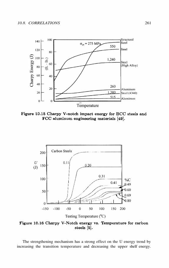
The strengthening mechanism has a strong effect on the U energy trend byincreasing the transition temperature and decreasing the upper shelf energy.
10.8. CORRELATIONS 261
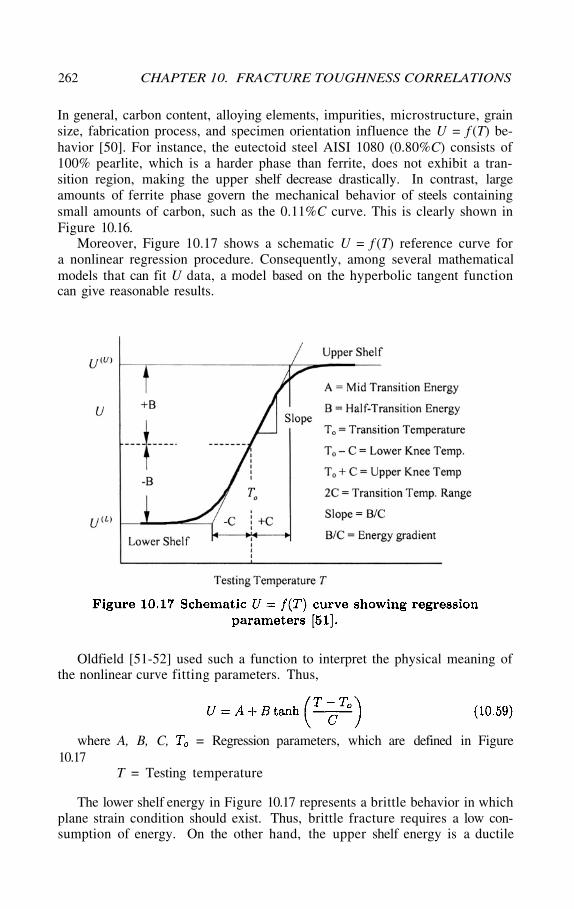
In general, carbon content, alloying elements, impurities, microstructure, grainsize, fabrication process, and specimen orientation influence the U = f (T) be-havior [50]. For instance, the eutectoid steel AISI 1080 (0.80%C) consists of100% pearlite, which is a harder phase than ferrite, does not exhibit a tran-sition region, making the upper shelf decrease drastically. In contrast, largeamounts of ferrite phase govern the mechanical behavior of steels containingsmall amounts of carbon, such as the 0.11%C curve. This is clearly shown inFigure 10.16.
Moreover, Figure 10.17 shows a schematic U = f (T) reference curve fora nonlinear regression procedure. Consequently, among several mathematicalmodels that can fit U data, a model based on the hyperbolic tangent functioncan give reasonable results.
Oldfield [51-52] used such a function to interpret the physical meaning ofthe nonlinear curve fitting parameters. Thus,
The lower shelf energy in Figure 10.17 represents a brittle behavior in whichplane strain condition should exist. Thus, brittle fracture requires a low con-sumption of energy. On the other hand, the upper shelf energy is a ductile
where A, B, C, = Regression parameters, which are defined in Figure10.17
T = Testing temperature
262 CHAPTER 10. FRACTURE TOUGHNESS CORRELATIONS
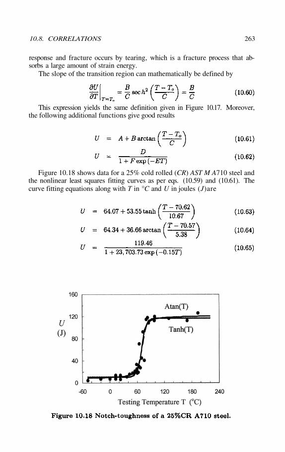
response and fracture occurs by tearing, which is a fracture process that ab-sorbs a large amount of strain energy.
The slope of the transition region can mathematically be defined by
This expression yields the same definition given in Figure 10.17. Moreover,the following additional functions give good results
Figure 10.18 shows data for a 25% cold rolled (CR) AST M A710 steel andthe nonlinear least squares fitting curves as per eqs. (10.59) and (10.61). Thecurve fitting equations along with T in °C and U in joules (J)are
10.8. CORRELATIONS 263
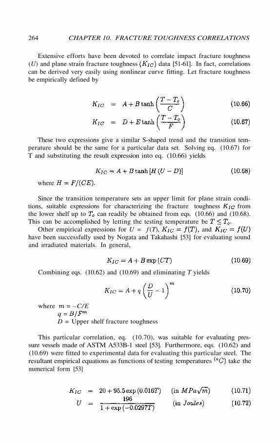
Extensive efforts have been devoted to correlate impact fracture toughness(U) and plane strain fracture toughness data [51-61]. In fact, correlationscan be derived very easily using nonlinear curve fitting. Let fracture toughnessbe empirically defined by
These two expressions give a similar S-shaped trend and the transition tem-perature should be the same for a particular data set. Solving eq. (10.67) forT and substituting the result expression into eq. (10.66) yields
where
Since the transition temperature sets an upper limit for plane strain condi-tions, suitable expressions for characterizing the fracture toughness fromthe lower shelf up to can readily be obtained from eqs. (10.66) and (10.68).This can be accomplished by letting the testing temperature be
Other empirical expressions for U = f (T), andhave been successfully used by Nogata and Takahashi [53] for evaluating soundand irradiated materials. In general,
Combining eqs. (10.62) and (10.69) and eliminating T yields
where = –C/Eq =D = Upper shelf fracture toughness
This particular correlation, eq. (10.70), was suitable for evaluating pres-sure vessels made of ASTM A533B-1 steel [53]. Furthermore, eqs. (10.62) and(10.69) were fitted to experimental data for evaluating this particular steel. Theresultant empirical equations as functions of testing temperatures take thenumerical form [53]
264 CHAPTER 10. FRACTURE TOUGHNESS CORRELATIONS
Combining eqs. (10.57) and (10.58) to eliminate T yields [53]
This expression, eq. (10.73), requires that otherwise,cannot be determined. Figure 10.19 shows the response of eq. (10.73) for thestructural steel type A533B-1. Observe that there is a linear correspondence inthe selected lower shelf energy.
For the upper energy shelf, the fracture toughness of the ASTM A723steel is correlated with both impact energy and yield strength [61]
where U is in Joules, in MPa and in
Other empirical correlations can be found in the literature. Of significanceis the Hertzberg’s book [62], which contains many compiled expressions in atabular form. Ideally, and U correlations should correspond to the sameloading rate, but quasi-static values can be estimated from dynamic Uexperimental data, taking into account the related temperature shift.
In this regard, a simple correlation for ABS-C, A302-B, and A517-F steelsin the transition region has been reported [61,63] to give conservative results.The reported mathematical expression is of the form
10.8. CORRELATIONS 265
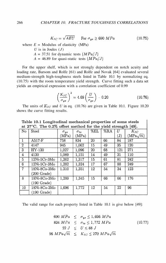
where E = Modulus of elasticity (MPa)U is in Joules (J )A = 37.51 for dynamic testsA = 46.89 for quasi-static tests
For the upper shelf, which is not strongly dependent on notch acuity andloading rate, Barsom and Rolfe [61) and Rolfe and Novak [64] evaluated severalmedium-strength high-toughness steels listed in Table 10.1 by normalizing eq.(10.75) with the room temperature yield strength. Curve fitting such a data setyields an empirical expression with a correlation coefficient of 0.99
The units of and U in eq. (10.76) are given in Table 10.1. Figure 10.20shows the curve fitting results.
The valid range for each property listed in Table 10.1 is give below [49]:
266 CHAPTER 10. FRACTURE TOUGHNESS CORRELATIONS
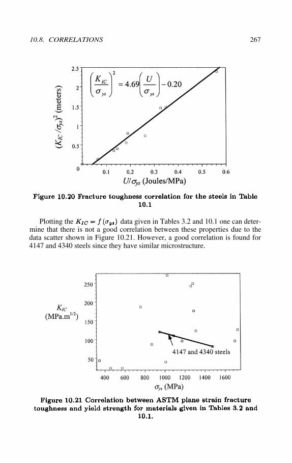
Plotting the data given in Tables 3.2 and 10.1 one can deter-mine that there is not a good correlation between these properties due to thedata scatter shown in Figure 10.21. However, a good correlation is found for4147 and 4340 steels since they have similar microstructure.
10.8. CORRELATIONS 267
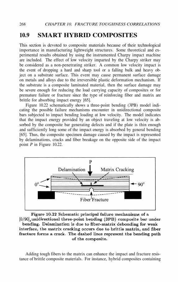
10.9 SMART HYBRID COMPOSITES
This section is devoted to composite materials because of their technologicalimportance in manufacturing lightweight structures. Some theoretical and ex-perimental results obtained by using the instrumented Charpy impact machineare included. The effect of low velocity imparted by the Charpy striker maybe considered as a non-penetrating striker. A common low velocity impact isthe event of dropping a hard and sharp tool or a falling bulk and heavy ob-ject on a substrate surface. This event may cause permanent surface damageon metals and alloys due to the irreversible plastic deformation mechanism. Ifthe substrate is a composite laminated material, then the surface damage maybe severe enough for reducing the load carrying capacity of composites or forpremature failure or fracture since the type of reinforcing fiber and matrix arebrittle for absorbing impact energy [65].
Figure 10.22 schematically shows a three-point bending (3PB) model indi-cating the possible failure mechanisms encounter in unidirectional compositebars subjected to impact bending loading at low velocity. The model indicatesthat the impact energy provided by an object traveling at low velocity is ab-sorbed by the composite bar generating defects and if the plate is thin enoughand sufficiently long some of the impact energy is absorbed by general bending[65]. Thus, the composite specimen damage caused by the impact is representedby delaminations, cracks and fiber breakage on the opposite side of the impactpoint P in Figure 10.22.
Adding tough fibers to the matrix can enhance the impact and fracture resis-tance of brittle composite materials. For instance, hybrid composites containing
268 CHAPTER 10. FRACTURE TOUGHNESS CORRELATIONS
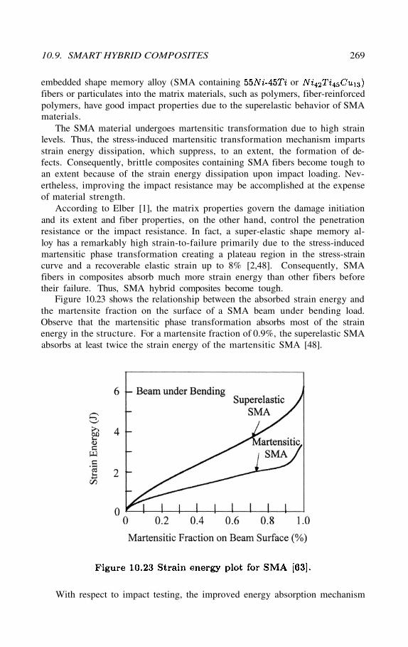
embedded shape memory alloy (SMA containing orfibers or particulates into the matrix materials, such as polymers, fiber-reinforcedpolymers, have good impact properties due to the superelastic behavior of SMAmaterials.
The SMA material undergoes martensitic transformation due to high strainlevels. Thus, the stress-induced martensitic transformation mechanism impartsstrain energy dissipation, which suppress, to an extent, the formation of de-fects. Consequently, brittle composites containing SMA fibers become tough toan extent because of the strain energy dissipation upon impact loading. Nev-ertheless, improving the impact resistance may be accomplished at the expenseof material strength.
According to Elber [1], the matrix properties govern the damage initiationand its extent and fiber properties, on the other hand, control the penetrationresistance or the impact resistance. In fact, a super-elastic shape memory al-loy has a remarkably high strain-to-failure primarily due to the stress-inducedmartensitic phase transformation creating a plateau region in the stress-straincurve and a recoverable elastic strain up to 8% [2,48]. Consequently, SMAfibers in composites absorb much more strain energy than other fibers beforetheir failure. Thus, SMA hybrid composites become tough.
Figure 10.23 shows the relationship between the absorbed strain energy andthe martensite fraction on the surface of a SMA beam under bending load.Observe that the martensitic phase transformation absorbs most of the strainenergy in the structure. For a martensite fraction of 0.9%, the superelastic SMAabsorbs at least twice the strain energy of the martensitic SMA [48].
With respect to impact testing, the improved energy absorption mechanism
10.9. SMART HYBRID COMPOSITES 269
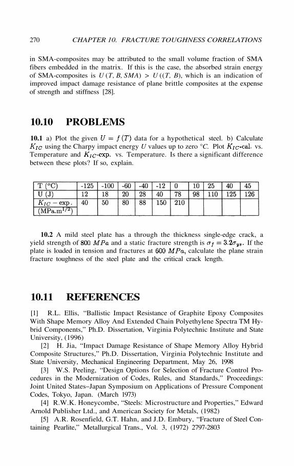
270 CHAPTER 10. FRACTURE TOUGHNESS CORRELATIONS
in SMA-composites may be attributed to the small volume fraction of SMAfibers embedded in the matrix. If this is the case, the absorbed strain energyof SMA-composites is U (T, B, S M A) > U ((T, B), which is an indication ofimproved impact damage resistance of plane brittle composites at the expenseof strength and stiffness [28].
10.10 PROBLEMS
10.1 a) Plot the given data for a hypothetical steel. b) Calculateusing the Charpy impact energy U values up to zero °C. Plot vs.
Temperature and vs. Temperature. Is there a significant differencebetween these plots? If so, explain.
10.2 A mild steel plate has a through the thickness single-edge crack, ayield strength of and a static fracture strength is If theplate is loaded in tension and fractures at calculate the plane strainfracture toughness of the steel plate and the critical crack length.
10.11 REFERENCES
[1] R.L. Ellis, “Ballistic Impact Resistance of Graphite Epoxy CompositesWith Shape Memory Alloy And Extended Chain Polyethylene Spectra TM Hy-brid Components,” Ph.D. Dissertation, Virginia Polytechnic Institute and StateUniversity, (1996)
[2] H. Jia, “Impact Damage Resistance of Shape Memory Alloy HybridComposite Structures,” Ph.D. Dissertation, Virginia Polytechnic Institute andState University, Mechanical Engineering Department, May 26, 1998
[3] W.S. Peeling, “Design Options for Selection of Fracture Control Pro-cedures in the Modernization of Codes, Rules, and Standards,” Proceedings:Joint United States–Japan Symposium on Applications of Pressure ComponentCodes, Tokyo, Japan. (March 1973)
[4] R.W.K. Honeycombe, “Steels: Microstructure and Properties,” EdwardArnold Publisher Ltd., and American Society for Metals, (1982)
[5] A.R. Rosenfield, G.T. Hahn, and J.D. Embury, “Fracture of Steel Con-taining Pearlite,” Metallurgical Trans., Vol. 3, (1972) 2797-2803
10.11. REFERENCES 271
[6] D.A. Curry and J.F. Knott, “The Relationship between Toughness andMicrostructure in the Cleavage Fracture of Mild Steel,” Metal Science, Vol. 10,(1976) 1-5
[7] R.O. Ritchie, J.F. Knott, and J.F. Rice, “On the Relation ship BetweenCritical Tensile Stress and Fracture Toughness in Mild Steel,” Journal of theMechanics and Physics of Solids, Vol. 21, (1973) 395-410
[8] E. Orowan, Trans. Inst. Eng. Shipbuild Scot., Vol. 89, (1945)[9] G.T. Hahn and A.R. Rosenfield, “Experimental Determination of Plastic
Constraint Ahead of a Sharp Notch under Plane-Strain Conditions,” Trans.ASM, Vol. 59, (1966) 909-919
[10] F.R. Stonesifer and R.W. Armstrong, “Effect of Prior Austenite GrainSize on the Fracture Toughness Properties of A533B Steel,” in Fracture 77, Vol.2A, Edited by D.M.R. Taplin, Pergamon Press (1977) 1-5
[11] M.W. Barsoum, “Fundamentals of Ceramics,” The McGraw-Hill Com-panies, Inc., New York, (1997) 404-405
[12] S. Palmquist, “Method of Determining the Toughness of Brittle Mate-rials, Particularly Sintered Carbides,” Jernkontorest Ann., Vol. 141 (5) (1957)300-307
[13] G.F. Vander Voort, “Metallography: Principles and Practice,” McGraw-Hill, Inc., New York, (1984) 350-389
[14] C.B. Ponton and R.D. Rawlings, “Vickers Indentation Fracture Tough-ness Test Part 1: Review of Literature and Formulation of Standardized In-dentation Toughness Equations,” Materials Sci. and Technology, Vol. 5, (Sept.1989) 965-872
[15] C.B. Ponton and R.D. Rawlings, “Dependence of the Vickers IndentationFracture Toughness on the Surface Crack Length,” Br. Ceramic Trans. J.,88(1989) 83-90
[16] K.K. Sharma, P.N. Kotru, and B.M. Wanklyn, “Microindentation Stud-ies of Flux-Grown ErFeO3 Single Crystals,” Applied Surface Science, Vol. 81(2) (Oct. 1994)
[17] M.T. Laugier, “Comparison of toughness in WC-Co determined by aCompact Tensile Technique with Model Predictions,” J. Mat. Sci. Letters, 6(1987) 779-780
[18] V. Milekhine, M.I. Onsoien, J.K. Solberg, and T. Skaland, “MechanicalProperties of and Elsevier, Intermetallics, 10 (2002)743-750
[19] G.R. Anstis, P. Chantikul, B.R. Lawn, and D.B. Marshall, J. Amer.Cer. Soc., 64(9), (1981) 533-538
[20] J. Phelps, J. Shields, X. Wang, and C.M. Agrawal, “Relationship ofFracture Toughness and Microstructural Anisotropy of Bone,” Southern Bio-medical Engineering Conference Proc., Sponsored by IEEE, (6-8 Feb. 1998)23
[21] A. Iost and R. Bigot, “Reply to comment on indentation size effect:reality or artifact?” J. Mat. Sci. Letters, Vol. 17 (22) (1998) 1889-1891
[22] K.K. Sharma, P.N. Kotru, and B.M. Wanklyn, “Microindentation Stud-ies of Flux-Grown ErFeO3 Single Crystal,” Applied Surface Sci., Vol. 18 (2)
272 CHAPTER 10. FRACTURE TOUGHNESS CORRELATIONS
(1994) 251-258[23] M.R. Sridhar and M.M. Yovanovich, “Empirical Methods to Predict
Vickers Microhardness,” Wear 193, (April 1996) 91-98[24] G. Berces, N.Q. Chinh, A. Juhasz, and J. Lendvai, “Kinetic Analysis of
Plastic Instabilities Occurring in Microhardness Tests,” Acta Mat., Vol. 46 (6)(23 March 1998) 2029-2037
[25] Z. Gurdal, R.T. Haftka, and P. Hajela, “Design and optimization oflaminated composite materials,” Wiley-Interscience, John Wiley & Sons, Inc.,(1999)
[26] R. M. Jones, “Mechanics of Composite Materials,” Book News, Inc.® ,Portland, OR, 2nd edition (June 1998)
[27] A. Hazizan and W.J. Cantwell, “The Low Velocity Impact Response ofFoam-Based Sandwich Structures,” Composites Part B: Vol. 33, No. 3, (2002)193-204
[28] J.S.N. Paine and C.A. Rogers, “The Response of SMA Hybrid Com-posite Materials to Low Velocity Impact,” J. Intelligent Material Systems andStructures, Vol. 5, (1994) 530-535
[29] W.J. Cantwell and J. Morton, “Geometrical Effects in the Low VelocityResponse of CFRP,” Composite Structures, Vol. 12, (1989) 39-59
[30] L. J. Broutman and A. Rotem, “Impact Strength and Toughness of FiberComposite Material,” ASTM STP 568, (1975) 114-133
[31] J.C. Aleszka, “Low Energy Impact Behavior of Composite Panels,” J.Test. Eval., 6 (3) (1978) 202-210
[32] M.P. Manahan, “In-situ Heating and Cooling of Charpy Test Speci-mens,” ASTM STP 1380, (1999)
[33] R.L. Ellis, F. Lalande, H. Jia and C.A. Rogers “Ballistic Impact Resis-tance of SMA and Spectra Hybrid Graphite Composites,” J. Reinf Plast andCompos, Vol. 17, 2 (1998) 147-164
[34] J.G. Hetherington and P.F. Lemieux, “The Effect of Obliquity on theBallistic Performance of Two Component Composite Armour,” Int. J. ImpactEngng Vol. 15, No. 2, (1994) 131-137
[35] J.D. Walker and C.E. Anderson, Jr., “The Influence of Initial NoseShape in Eroding Penetration,” Int. J. Impact Engng Vol. 15, No. 2, (1994)139-148
[36] W.J. Cantwell and J. Morton, “Comparison of the Low and High Ve-locity Impact Response of CFRP,” Composites, Vol. 20, No. 6 (1989) 545-551
[37] M.P. Manahan and R.B. Stonesifer, “Studies Toward Optimum Instru-mented Striker Designs,” MPM Technologies, Inc., State College, PA 16803
[38] H.W. Hayden, W.G. Moffatt, and J. Wulff, “The Structure and Prop-erties of Materials,” Vol. III, Mechanical Behavior, John Wiley & Sons, (1965)
[39] MPM Technologies, Inc., www.mpmtechnologies.com, (2003)[40] M.P. Manahan, “Advances in Notched Bar Impact Testing,” ASTM
Standardization News, (October 1996) 23-29[41] H.J. Schindler, T. Varga, H. Njo, and G. Prantl, “Key Issues of In-
strumented Pre-cracked Charpy-Type Testing in Irradiation Surveillance Pro-
10.11. REFERENCES 273
grams,” Proc. Int. Symposium on Materials Aging and Component Life Exten-sion, Milan, Italy, Vol. II, (10-13 October 1995) 1367-1377
[42] H.J. Schindler, “The Use of Instrumented Pre-cracked Charpy Speci-mens,” Engineering Integrity Assessment Evaluating Material Properties by Dy-namic Testing, ESIS 20, Mechanical Engineering Publications, London, (1996)45-58
[43] H.J. Schindler, “Estimation of the Dynamic JR Curve from a SingleImpact Bending Test,” Proc. ECF 11 – Mechanical and Mechanics of Damagedand Failure, Vol. II, Editor J. Petit, EMAS Publishing, (1996) 2007-2012
[44] H.J. Schindler and M. Veidt, “Fracture Toughness Evaluation from In-strumented Sub-size Charpy-Type Tests,” ASTM STP 1329, (1997) 48-62
[45] W. Böhme and H.J. Schindler, “Application of Single-Specimen Meth-ods on Instrumented Charpy Tests: Results of DVM Round-Robin Exercises,”ASTM STP 1380, (1999) 327-336
[46] H.J. Schindler, “Preferable Initial Length for Fracture Toughness Eval-uation Using Sub-sized Bend Specimens,” ASTM STP 1418, (2002) 67-79
[47] J.G. Williams, “Fracture Mechanics of Polymers,” Ellis Horwood Lim-ited Publishers, Halsted Press a division of John Wiley & Sons, New York,(1984)
[48] W.F. Brown and J.E. Strawley, ASTM STP 410, (1966)[49] J.M. Barsom and S.T. Rolfe, “Fracture and Fatigue in Structure: Ap-
plication of fracture Mechanics,” Third edition, American Society for Testingand Materials Philadelphia, PA, (1999)
[50] Metals Handbook, Edited by H.E. Boyer and T.L. Gall, American So-ciety for Metals (ASM) (1985)
[51] W. Oldfield, “Curve Fitting Impact Test Data: A Statistical Procedure,”ASTM Standardization News, Vol. 3, No. 11, (Nov. 1975) 24-29
[52] W. Oldfield, “Fitting Curves to Toughness Data,” J. Testing and Eval-uation, JTEVA, Vol. 7, No. 6, (Nov. 1979) 326-333
[53] F.N. Nogata and H. Takahashi, “Fracture Mechanics Evaluation of Ir-radiated Embrittlement in Reactor Vessel Steels Based on the Rate ProcessConcept,” J. Testing and Evaluation, JTEVA, Vol. 14, No. 1, (Jan. 1986).40-48
[54] J.D. Varsik and S.T. Byrne, “An Empirical Evaluation of the IrradiationSensitivity of Reactor Pressure Vessel Materials,” ASTM STP 683, (1979) 252-266
[55] R.H. Sailors and H.T. “Relationship Between Material Fracture Tough-ness Using Fracture Mechanics and Transition Temperature Tests,” ASTM STP514 (1972) 164-191
[56] S. Tauscher, “The Correlation of Fracture Toughness with Charpy V-Notch Impact Test Data,” USA ARRADCOM Technical Report ARLCB-TR-81012, Benet Weapons Laboratory, Waterviliet, NY, (March 1977)
[57] J.A. Kapp and J.H. Underwood, “Correlations between Fracture Tough-ness, Charpy V-Notch, and Yield Strength for ASTM A723 Steel,” ASME, Pres-sure Vessels & Piping Division, (June 21-25, (1992) 219-221
274 CHAPTER 10. FRACTURE TOUGHNESS CORRELATIONS
[58] B. Nageswara and A.R. Acharya, “Comparative Study on Evaluationof Fracture Toughness from Charpy V-Notch Impact Energy and Reduction inArea,” Eng. Fracture Mechanics (Jan. 1992) 85-90
[59] J.H. Underwood and G.S. Leger, “Fracture Toughness of High StrengthSteel Predicted from Charpy Energy or Reduction in Area,” ASTM STP 833,(1984) 481-498.
[60] S.T. Rolfe, W.A. Sorem, and G.W. Wellman, “Fracture Control in theTransition-Temperature Region of Structural Steels,” J. Constructional SteelRes. (1989) 171-195
[61] J.M. Barsom and S.T. Rolfe, “Correlations Between and CharpyV-Notch Test Results in the Transition-Temperature Range,” ASTM STP 466,(1970) 281-302
[62] R. W. Herztberg, “Deformation and Fracture Mechanics of EngineeringMaterials,” Third Edition, John Wiley & Sons, Inc., (1989)
[63] J.M. Barsom, “The Development of AASHTO Fracture Toughness Re-quirements for Bridge Steels,” Engineering Fracture Mechanics, Vol. 7, No. 3,(Sept. 1975) 605-618
[64] S.T. Rolfe and S.R. Novak, “Slow-Bend Testing of Medium StrengthHigh-Toughness Steels,” ASTM STP 463 (1970) 124-159
[65] W. Elber, “Effect of Matrix and Fiber Properties on Impact Resistance,”Tough Composite Materials: Recent developments, Noyes, Park Ridge, NJ,(1985) 89-110
[66] M.P. Manahan and R.B. Stonesifer, “The Difference Between Total Ab-sorbed Energy measured Using an Instrumented Striker and that Obtained Us-ing an Optical Encoder,” ASTM STP 1380, (1999)
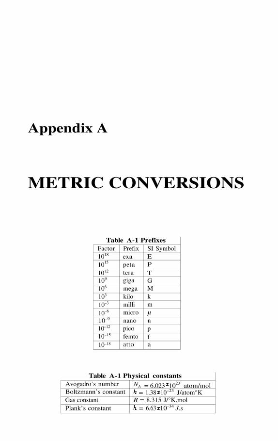
Appendix A
METRIC CONVERSIONS
Table A-1 PrefixesFactor1018
1015
1012
109
106
103
10–3
10–6
10–9
10–12
10–15
10–18
Prefixexapetateragigamegakilomillimicronanopicofemtoatto
SI SymbolEPTGMkm
npfa
Table A-1 Physical constantsAvogadro’s numberBoltzmann’s constantGas constantPlank’s constant
NA = 6.023 1023 atom/mol= 1.38 10–23 J/atom°K
R = 8.315 J/°K.mol= 6.63 10–34 J.s
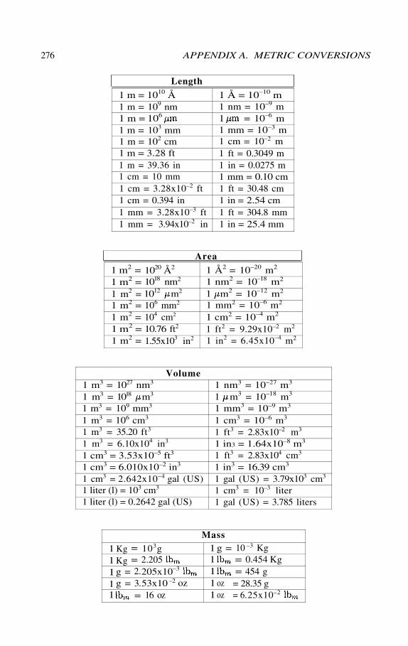
276 APPENDIX A. METRIC CONVERSIONS
Length
1 m = 1010 Å1 m = 109 nm1 m = 106
1 m = 103 mm1 m = 102 cm1 m = 3.28 ft1 m = 39.36 in1 cm = 10 mm1 cm = 3.28x10⁻² ft1 cm = 0.394 in1 mm = 3.28x10⁻³ ft1 mm = 3.94x10⁻² in
1 Å = 10–10 m1 nm = 10–9 m1 = 10–6 m1 mm = 10–3 m1 cm = 10–2 m1 ft = 0.3049 m1 in = 0.0275 m1 mm = 0.10 cm1 ft = 30.48 cm1 in = 2.54 cm1 ft = 304.8 mm1 in = 25.4 mm
Area
1 m2 =1 m2 =1 m2 =1 m2 =1 m2 =1 m2 =1 m2 =
1020 Å2
1018 nm2
1012 m2
106 mm2
104 cm2
10.76 ft2
1.55x10³ in2
1 Å2 = 10–20 m2
1 nm2 = 10–18 m2
1 m2 = 10–12 m2
1 mm2 = 10–6 m2
1 cm2 = 10–4 m2
1 ft2 = 9.29x10⁻² m2
1 in2 = 6.45x10⁻⁴ m2
Volume1 m3 = 1027 nm3
1 m3 = 1018 m3
1 m3 = 109 mm3
1 m3 = 106 cm3
1 m3 = 35.20 ft3
1 m3 = 6.10x10⁴ in3
1 cm3 = 3.53x10⁻⁵ ft3
1 cm3 = 6.010x10⁻² in3
1 cm3 = 2.642x10⁻⁴ gal (US)1 liter (l) = 103 cm3
1 liter (l) = 0.2642 gal (US)
1 nm3 = 10–27 m3
1 m3 = 10–18 m3
1 mm3 = 10–9 m3
1 cm3 = 10–6 m3
1 ft3 = 2.83x10⁻² m3
1 in3 = 1.64x10⁻⁸ m3
1 ft3 = 2.83x104 cm3
1 in3 = 16.39 cm3
1 gal (US) = 3.79x103 cm3
1 cm3 = 10–3 liter1 gal (US) = 3.785 liters
Mass
11111
KgKgg =g =
==2.3.=
103g2.205205x10–3
53x1016 oz
–2 oz
11111
g =
ozoz
10==
–3 Kg0.454 Kg454 g
= 28.35 g= 6.25x10⁻²
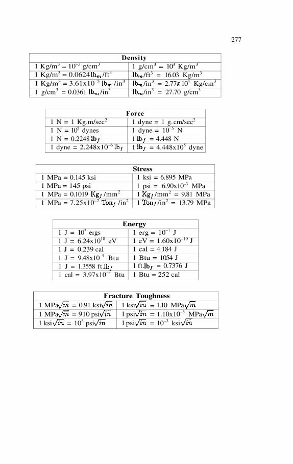
277
Density1 Kg/m3 = 10–3 g/cm3
1 Kg/m3 = 0.0624 /ft3
1 Kg/m3 = 3.61x10⁻⁵ /in3
1 g/cm3 = 0.0361 /in3
1 g/cm3 = 103 Kg/m3
/ft3 = 16.03 Kg/m3
/in3 = 2.77 104 Kg/cm3
/in3 = 27.70 g/cm3
Force1 N = 1 Kg.m/sec2
1 N = 105 dynes1 N = 0.22481 dyne = 2.248x10⁻⁶
1 dyne = 1 g. cm/sec2
1 dyne = 10–5 N1 = 4.448 N1 = 4.448x10⁵ dyne
Stress1 MPa = 0.145 ksi1 MPa = 145 psi1 MPa = 0.1019 /mm2
1 MPa = 7.25x10⁻² /in2
1 ksi = 6.895 MPa1 psi = 6.90x10⁻³ MPa1 /mm2 = 9.81 MPa1 /in2 = 13.79 MPa
Energy1 J = 107 ergs1 J = 6.24x10¹⁸ eV1 J = 0.239 cal1 J = 9.48x10⁻⁴ Btu1 J = 1.3558 ft.1 cal = 3.97x10⁻³ Btu
1 erg = 10–7 J1 eV = 1.60x10⁻¹⁹ J1 cal = 4.184 J1 Btu = 1054 J1 ft. = 0.7376 J1 Btu = 252 cal
Fracture Toughness1 MPa = 0.91 ksi1 MPa = 910 psi1 ksi = 103 psi
1 ksi1 psi =1 psi =
1.10 MPa1.10x10–3 MPa10–3 ksi
=
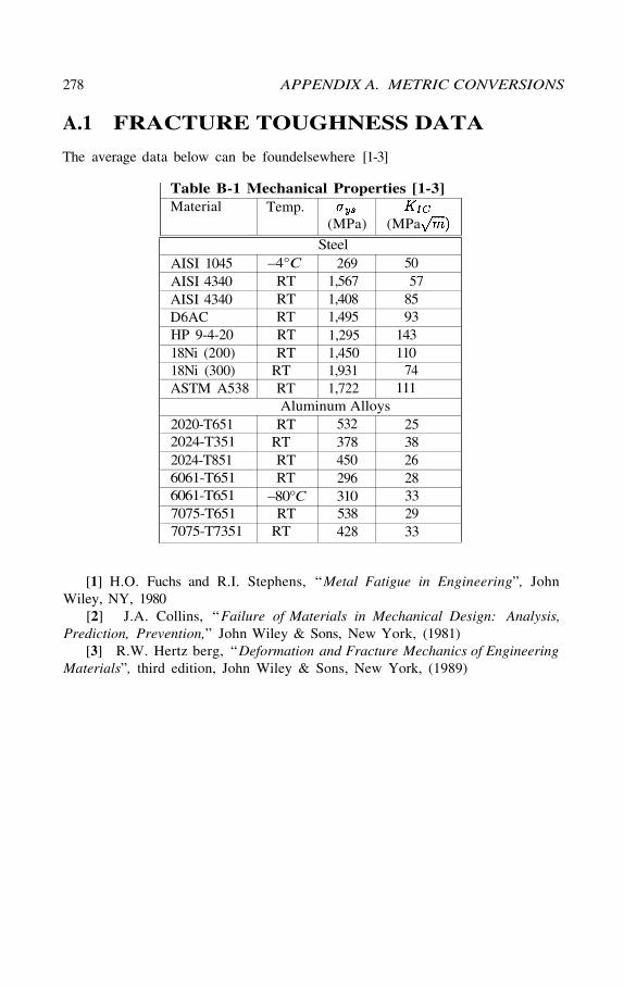
278 APPENDIX A. METRIC CONVERSIONS
A.1 FRACTURE TOUGHNESS DATA
The average data below can be foundelsewhere [1-3]
Table B-1 Mechanical Properties [1-3]Material Temp.
(MPa) (MPa
SteelAISI 1045AISI 4340AISI 4340D6ACHP 9-4-2018Ni (200)18Ni (300)ASTM A538
–4°CRTRTRTRTRT
RTRT
2691,5671,4081,4951,2951,4501,9311,722
5057
8593
143110
74111
Aluminum Alloys2020-T6512024-T3512024-T8516061-T6516061-T6517075-T6517075-T7351
RTRTRTRT
–80°CRT
RT
532378450296310538428
25382628332933
[1] H.O. Fuchs and R.I. Stephens, “Metal Fatigue in Engineering”, JohnWiley, NY, 1980
[2] J.A. Collins, “Failure of Materials in Mechanical Design: Analysis,Prediction, Prevention,” John Wiley & Sons, New York, (1981)
[3] R.W. Hertz berg, “Deformation and Fracture Mechanics of EngineeringMaterials”, third edition, John Wiley & Sons, New York, (1989)
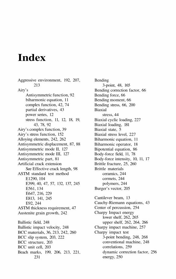
Index
Aggressive environment, 192, 207,213
Airy’sAntisymmetric function, 92biharmonic equation, 11complex function, 42, 74partial derivatives, 43power series, 12stress function, 11, 12, 18, 19,
43, 78, 92Airy’s complex function, 39Airy’s stress function, 152Alloying elements, 242, 262Antisymmetric displacement, 87, 88Antisymmetric mode II, 127Antisymmetric mode III, 127Antisymmetric part, 81Artificial crack extension
See Effective crack length, 98ASTM standard test method
E1290, 104E399, 40, 47, 57, 132, 137, 245E561, 134E647, 216, 229E813, 141, 245E92, 244
ASTM thickness requirement, 47Austenite grain growth, 242
Ballistic field, 248Ballistic impact velocity, 248BCC materials, 36, 213, 242, 260BCC slip system, 203, 222BCC structure, 203BCC unit cell, 203Beach marks, 199, 206, 213, 221,
231
Bending3-point, 48, 165
Bending correction factor, 66Bending force, 66Bending moment, 66Bending stress, 66, 200Biaxial
stress, 44Biaxial cyclic loading, 227Biaxial loading, 181Biaxial state, 5Biaxial stress level, 227Biharmonic equation, 11Biharmonic operator, 18Bipotential equation, 86Body-force field, 11, 78Body-force intensity, 10, 11, 17Brittle fracture, 25, 260Brittle materials
ceramics, 244cermets, 244polymers, 244
Burger’s vector, 205
Cantilever beam, 13Cauchy-Riemann equations, 43Center of percussion, 254Charpy Impact energy
lower shelf, 262, 265upper shelf, 262, 264, 266
Charpy impact machine, 257Charpy impact test
3-point bending, 248, 268conventional machine, 248correlations, 259dynamic correction factor, 256energy, 250
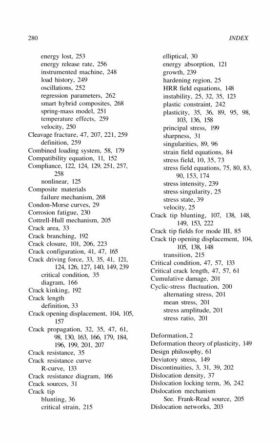
280 INDEX
energy lost, 253energy release rate, 256instrumented machine, 248load history, 249oscillations, 252regression parameters, 262smart hybrid composites, 268spring-mass model, 251temperature effects, 259velocity, 250
Cleavage fracture, 47, 207, 221, 259definition, 259
Combined loading system, 58, 179Compatibility equation, 11, 152Compliance, 122, 124, 129, 251, 257,
258nonlinear, 125
Composite materialsfailure mechanism, 268
Condon-Morse curves, 29Corrosion fatigue, 230Cottrell-Hull mechanism, 205Crack area, 33Crack branching, 192Crack closure, 101, 206, 223Crack configuration, 41, 47, 165Crack driving force, 33, 35, 41, 121,
124, 126, 127, 140, 149, 239critical condition, 35diagram, 166
Crack kinking, 192Crack length
definition, 33Crack opening displacement, 104, 105,
157Crack propagation, 32, 35, 47, 61,
98, 130, 163, 166, 179, 184,196, 199, 201, 207
Crack resistance, 35Crack resistance curve
R-curve, 133Crack resistance diagram, 166Crack sources, 31Crack tip
blunting, 36critical strain, 215
elliptical, 30energy absorption, 121growth, 239hardening region, 25HRR field equations, 148instability, 25, 32, 35, 123plastic constraint, 242plasticity, 35, 36, 89, 95, 98,
103, 136, 158principal stress, 199sharpness, 31singularities, 89, 96strain field equations, 84stress field, 10, 35, 73stress field equations, 75, 80, 83,
90, 153, 174stress intensity, 239stress singularity, 25stress state, 39velocity, 25
Crack tip blunting, 107, 138, 148,149, 153, 222
Crack tip fields for mode III, 85Crack tip opening displacement, 104,
105, 138, 148transition, 215
Critical condition, 47, 57, 133Critical crack length, 47, 57, 61Cumulative damage, 201Cyclic-stress fluctuation, 200
alternating stress, 201mean stress, 201stress amplitude, 201stress ratio, 201
Deformation, 2Deformation theory of plasticity, 149Design philosophy, 61Deviatory stress, 149Discontinuities, 3, 31, 39, 202Dislocation density, 37Dislocation locking term, 36, 242Dislocation mechanism
See. Frank-Read source, 205Dislocation networks, 203

INDEX 281
Displacement, 2, 3, 22, 26, 76, 84,87, 105, 121, 124, 126, 130,255
cumulative, 207for slender cantilever beam, 129mode I, 126mode II, 127mode III, 127vector, 135
Displacement field equations, 76, 79,85, 174, 175
Dissipation function, 255Dissipation of energy, 269Ductile fracture, 25Ductile-to-brittle transition, 259, 260Ductility, 7, 9, 63, 155, 239, 241, 242Dugdale’s approximation, 101
behavior, 103Dynamic effects, 251Dynamic test, 248, 259
Effective crack length, 98, 104, 134,158, 164
Effective stress, 149for plane strain, 150for plane stress, 150
Effective stress intensity factor, 95,100, 227
Effective stress intensity factor range,227
Eigenvalue, 80, 81, 87Eigenvalue function, 80Elastic behavior, 8Elastic strain energy density, 8Elastic surface energy, 33, 34Elastic unloading, 148Elliptical fracture criterion, 179Energy losses, 254Energy principle, 121Energy release rate, 121Engineering strain, 6Equilibrium equations, 10Equivalent stress, 152Extrusions, 199
Far-field J-integral, 163
Fatigue crack growth, 207Fatigue crack growth rate, 207
for BCC materials, 216for FCC materials, 216for polymers, 217for weldments, 218measurements, 229
Fatigue crack initiation, 203Fatigue failure
appearance, 220prevention, 202stage I, 205, 207, 212, 213, 220stage II, 206–208, 213, 215, 216,
219–221, 231stage III, 207, 213, 215
Fatigue fracture, 206Fatigue life, 209Fatigue life, definition, 200FCC materials, 213, 260Fracture angle, 179Fracture control, 60Fracture process zone, 96, 122, 126,
141, 148, 155, 158Fracture toughness, 7, 9, 239–242
Charpy, 248, 250, 264COD, 104correlations, 239, 264criterion, 137critical value, 33CTOD, 104, 107data, 62energy release rate, 35, 36J-integral, 136, 137, 139, 141,
149, 155mixed-mode, 177, 179mode II, 187Plane strain, 57plane strain, 47, 61, 63, 64, 134,
177, 207, 245–247, 264upper energy shelf, 265
plane stress, 57, 246ratio, 183thickness dependency, 62Vickers, 244–246
Fracture toughness correlation
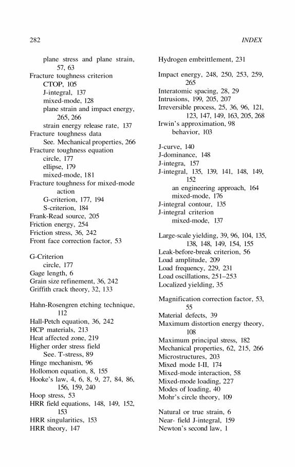
282 INDEX
plane stress and plane strain,57, 63
Fracture toughness criterionCTOP, 105J-integral, 137mixed-mode, 128plane strain and impact energy,
265, 266strain energy release rate, 137
Fracture toughness dataSee. Mechanical properties, 266
Fracture toughness equationcircle, 177ellipse, 179mixed-mode, 181
Fracture toughness for mixed-modeaction
G-criterion, 177, 194S-criterion, 184
Frank-Read source, 205Friction energy, 254Friction stress, 36, 242Front face correction factor, 53
G-Criterioncircle, 177
Gage length, 6Grain size refinement, 36, 242Griffith crack theory, 32, 133
Hahn-Rosengren etching technique,112
Hall-Petch equation, 36, 242HCP materials, 213Heat affected zone, 219Higher order stress field
See. T-stress, 89Hinge mechanism, 96Hollomon equation, 8, 155Hooke’s law, 4, 6, 8, 9, 27, 84, 86,
156, 159, 240Hoop stress, 53HRR field equations, 148, 149, 152,
153HRR singularities, 153HRR theory, 147
Hydrogen embrittlement, 231
Impact energy, 248, 250, 253, 259,265
Interatomic spacing, 28, 29Intrusions, 199, 205, 207Irreversible process, 25, 36, 96, 121,
123, 147, 149, 163, 205, 268Irwin’s approximation, 98
behavior, 103
J-curve, 140J-dominance, 148J-integra, 157J-integral, 135, 139, 141, 148, 149,
152an engineering approach, 164mixed-mode, 176
J-integral contour, 135J-integral criterion
mixed-mode, 137
Large-scale yielding, 39, 96, 104, 135,138, 148, 149, 154, 155
Leak-before-break criterion, 56Load amplitude, 209Load frequency, 229, 231Load oscillations, 251–253Localized yielding, 35
Magnification correction factor, 53,55
Material defects, 39Maximum distortion energy theory,
108Maximum principal stress, 182Mechanical properties, 62, 215, 266Microstructures, 203Mixed mode I-II, 174Mixed-mode interaction, 58Mixed-mode loading, 227Modes of loading, 40Mohr’s circle theory, 109
Natural or true strain, 6Near- field J-integral, 159Newton’s second law, 1
INDEX 283
Nil-ductility-transition temperature,259
Nitinol, 8, 240Nonlinear fracture mechanism, 148Nonlinear regression, 262Normal strains, 3
Opening mode I, 40
Paris law, 208Penny-shaped crack, 52Plane strain condition, 10, 75, 96
controlling parameter, 12, 33,41, 85, 99, 105, 127, 128,156, 164, 176
Plane strain fracture toughness, 239Plane stress condition, 10, 75, 96
controlling parameter, 12, 33,41, 85, 99, 105, 127, 128,156, 164, 176
Plastic constraint factor, 242Plastic deformation energy, 34Plastic zone shape, 107, 109, 110
photomicrographs, 112schematic, 96
Plastic zone size, 35, 39, 63, 73, 76,89, 96, 98, 126, 148, 151–153, 156, 184
approximation, 107Dugdale’s model, 101equation, 97equation for mode III, 100Irwin’s equation, 100schematic, 184stress state, 96Tresca equation, 109von Mises equation, 108
Principal strains, 6Principal stresses, 5Principle of superposition, 4, 65, 102Product method, 80
Ramberg-Osgood equation, 8, 155Resilience, 8Rotational velocity, 254
S-N diagram, 201
Safety factor, 2Second-rank tensors, 3Secondary cracks, 230Shape factor, 53Shape memory alloy, 240, 269Shear lip, 220Shear modulus, 3Shear strains, 3Shedding loads, 98Skew-symmetric loading, 173Sliding mode II, 40SMA fibers, 269SMA hybrid composites, 269Small-scale yielding, 39, 96, 104, 133,
135, 138, 155Space lattice, 203Stable crack growth, 149Strain, 2, 4Strain energy density, 136Strain energy density, total, 9Strain energy release rate, 34
mixed-mode, 176Strain hardening exponent, 8, 125,
150Strain-energy release rate
approximation, 107Strength, 2Stress, 2, 4Stress biaxiality, 89Stress biaxiality ratio, 90, 92Stress concentration factor, 30, 31Stress corrosion cracking, 230Stress field equations, 175, 176
for Mode I and II, 90Stress intensity factor, 33, 39
Dugdale’s equation, 103SCC, 232transition, 216
Stress intensity factor range, 208Stress-intensity factor, 31, 33, 34Stress-strain curves, 7, 150, 239Striations, 199, 206, 207, 213, 221,
231formation, 222in Al-alloy, 223lack of, 224
284 INDEX
mechanism, 221perturbations, 224ripples, 223size, 224
Surfaces fracture appearance, 220Symmetric circular hole, 31Symmetric loading, 200, 201Symmetric mode I, 126Symmetric part, 81Symmetrical arrays of atoms, 28
T-stress, 90, 92, 93Taylor’s series, 52Tearing mode III, 40Tearing modulus, 140Theoretical strength, 26, 27Theory of indentation, 244Thoeretical fracture strength, 27Threshold stress intensity factor, 207Traction forces, 126, 135, 136Translational velocity, 254Tresca criterion, 97Tresca yielding criterion, 109Triaxial stress state, 4
Unstable crack growth, 149
Vickers fracture toughness, 245Virtual crack length
See Effective crack length, 98Virtual crack size
See Effective crack length, 104Void coalescence, 98, 104, 133, 148,
150Von Mises yielding criterion, 108
Wedge internal forces, 101Welding cracks, 219Welding zones, 219Weldments, 218Westergaard’s complex function, 39,
42, 44, 45, 73, 77Westergaard’s stress function, 44Windage energy, 254
Yield strength
See. Table 3.2, 10.1 and Ap-pendix A, 62
Yielding, 25, 36