Serie Statistica

n. 2/2011

Silvia Figini, Lijun Gao, Paolo Giudici

Bayesian efficient capital at risk estimation

QUADERNI DEL DIPARTIMENTO DI ECONOMIA, STATISTICA E DIRITTO UNIVERSITÀ DI PAVIA ______________________________________________________________________ REDAZIONE Claudia Banchieri Dipartimento di Economia, Statistica e Diritto Università degli Studi di Pavia Corso Strada Nuova 65 27100 PAVIA tel. 0039-0382-984406 fax 0039-0382-984402 E-MAIL banchier@unipv.it I Quaderni sono disponibili sul sito: http://www-5.unipv.it/webdesed/quaderni.php COMITATO SCIENTIFICO Italo Magnani (coordinatore) Luigi Bernardi Silvia Cipollina Paolo Giudici Silvia Illari Renata Targetti Lenti I QUADERNI DEL DIPARTIMENTO DI ECONOMIA, STATISTICA E DIRITTO hanno lo scopo di favorire la tempestiva divulgazione, in forma provvisoria o definitiva, di ricerche scientifiche originali. La pubblicazione di lavori nella collana è soggetta a referaggio e all’approvazione del Comitato Scientifico. Questa nuova edizione dei QUADERNI rappresenta la continuazione di tre serie di pubblicazioni pre-esistenti: Quaderni del Dipartimento di Economia Pubblica e Territoriale, Quaderni di ricerca del Dipartimento di Statistica ed Economia Applicate “L. Lenti” e Osservatorio dei contratti della P.A.

Bayesian efficient capital at risk estimation

Silvia Figini∗Lijun Gao†and Paolo Giudici‡

May 11, 2011

Abstract: Operational risk is hard to quantify for the deficiency of lossdata and the presence of fat-tailed distribution. Extreme value distributions areconventionally used in such context. However, such distributions are very sen-sitive to the data and this may be a problem when data are scarce, as it occursin operational risk management. To overcome this problem, in this paper wepropose Bayesian extreme value models for operational risk management, usingboth non-informative and informative prior distributions.We test the proposed models on two real databases. One is an external databasethat contains loss data of Chinese commercial banks, the other is an internal lossdatabase of an anonymous European bank. For the Chinese database, there isno prior information available and, on the basis of an extensive sensitivity anal-ysis, we provide appropriate prior specification for both frequency and severitydistributions.For the European database, instead, we have prior information available frominternal self assessment and, therefore, we can compare uninformative with in-formative prior Bayesian models.To assess our models, and compare it with classical ones, we also derive poste-rior predictive distributions for both loss frequency and severity and, therefore,we backtest the estimate of capital at risk obtained under different models. Theobtained results show that, for both applications, Bayesian models perform bet-ter with respect to classical extreme value models, as they lead to a smallerquantification of capital at risk required to cover losses.

Keywords: Bayesian risk models, Extreme value distributions, Opera-tional risk management, Self assessment prior distributions.

1 Introduction

In this paper we improve the state of the art on statistical models for risk mea-surement (see e.g. Behrens et al. 2006). Recently there has been a rapid and

∗Department of Ecomomics, Statistics and Law, University of Pavia, silvia.figini@unipv.it†Management School, Shandong University of Finance, Jinan, China‡Department of Ecomomics, Statistics and Law, University of Pavia, Italy

1

widespread development of models for a new category of financial risks: oper-ational risks. This is due not only to regulatory compliance, but also to therecognition of the fact that business complexity and sophistication need a cor-rect evaluation for this type of risk as well.According to regulatory terminology (see e.g. www.bis.org), we focus our atten-tion on the advanced measurement approach (AMA) and in particular, on theloss distribution approach (LDA). These approaches can give greater flexibilityin comparison with traditional accounting approaches, as they take into accountthe particular characteristics of banking institutions: for example, they measurethe capital at risk on the basis of the classification of operational losses in busi-ness line/event type (BL/ET, see e.g. Dalla Valle and Giudici, 2008, Figini etal. 2010, Figini et al. 2010, Figini et al. 2007).The objective of the present work is to introduce a novel LDA method to esti-mate the capital at risk required to cover operational losses. Our proposed modelis derived under a Bayesian paradigm. More precisely, we extend Behrens et al.(2006) considering a convolution between the loss frequency and severity distri-butions. Prior distributions are elicited for the parameters of both distributions,under two different settings: an uninformative prior setting, when expert opin-ions are not available, and an informative prior setting, build exploiting expertopinions specified by means of a self assessment process (see e.g. Bonafede andGiudici, 2007, Bilotta and Giudici, 2004).Bayesian estimation of the parameters is provided through Markov Chain MonteCarlo (see e.g. Gamerman, 1997). We then obtain the predicted total loss dis-tribution and therefore compute a capital at risk measure (see e.g. Artzner etal., 1999), such as the Value at Risk (VaR) and the Expected Shortfall (ES).We shall compare the results achieved in our Bayesian framework with thoseobtained under a classical extreme value model based on a Poisson distributionfor the frequency and a generalized Pareto distribution for the severity (see e.g.Demoulin et al., 2006).The paper is organized as follows: Section 2 reports the classical extreme valuemodel; Section 3 introduces our proposed Bayesian model; Section 4 describesthe real data at hand and underlines the empirical evidences obtained using bothclassical and Bayesian approaches. Section 5 ends with concluding remarks andfurther ideas of research.

2 Classical Extreme Value models for operationalrisk

Extreme Value Theory (EVT) is considered a useful statistical tool for analyzingrare events: operational risk data exhibit properties, such as heavy tails, which,in natural way, call for EVT analysis. In EVT models, the peak over thresholdprocedure is a method which can solve data the parameter estimation problem.The procedure builds upon results of Balkema and de Haan (1974) and Pickands(1975) who show that, for a broad class of distributions, the distribution values

2

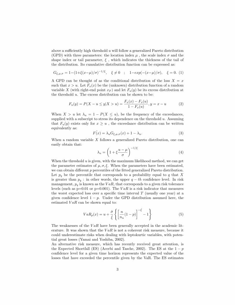
above a sufficiently high threshold u will follow a generalized Pareto distribution(GPD) with three parameters: the location index µ , the scale index σ and theshape index or tail parameter, ξ , which indicates the thickness of the tail ofthe distribution. Its cumulative distribution function can be expressed as:

Gξ,µ,σ = 1−(1+ξ(x−µ)/σ)−1/ξ, ξ 6= 0 ; 1−exp(−(x−µ)/σ), ξ = 0. (1)

A GPD can be thought of as the conditional distribution of the loss X = xsuch that x > u. Let Fx(x) be the (unknown) distribution function of a randomvariable X (with right-end point xF ) and let Fu(y) be its excess distribution atthe threshold u. The excess distribution can be shown to be:

Fu(y) = P (X − u ≤ y|X > u) =Fx(x)− Fx(u)

1− Fx(u), y = x− u (2)

When X > u let λu = 1 − P (X ≤ u), be the frequency of the exceedances,supplied with a subscript to stress its dependence on the threshold u. Assumingthat Fu(y) exists only for x ≥ u , the exceedance distribution can be writtenequivalently as:

ˆF (x) = λuGξ,µ,σ(x) + 1− λu. (3)

When a random variable X follows a generalized Pareto distribution, one caneasily obtain that:

λu =(

1 + ξu− µσ

)−1/ξ

(4)

When the threshold u is given, with the maximum likelihood method, we can getthe parameter estimates of µ, σ, ξ. When the parameters have been estimated,we can obtain different p percentiles of the fitted generalized Pareto distribution.Let pq be the percentile that corresponds to a probability equal to q that Xis greater than pq : in other words, the upper q − th confidence level. In riskmanagement, pq is known as the V aR, that corresponds to a given risk tolerancelevels (such as p=0.01 or p=0.001). The V aR is a risk indicator that measuresthe worst expected loss over a specific time interval T (usually one year) at agiven confidence level 1 − p. Under the GPD distribution assumed here, theestimated V aR can be shown equal to:

V aRp(x) = u+σ̂

ξ̂

{[n

nu(1− p)

]−ξ̂− 1

}(5)

The weaknesses of the V aR have been generally accepted in the academic lit-erature. It was shown that the V aR is not a coherent risk measure, because itcould underestimate risks when dealing with leptokurtic variables, with poten-tial great losses (Yamai and Yoshiba, 2002).An alternative risk measure, which has recently received great attention, isthe Expected Shortfall (ES) (Acerbi and Tasche, 2002). The ES at the 1 − pconfidence level for a given time horizon represents the expected value of thelosses that have exceeded the percentile given by the VaR. The ES estimates

3

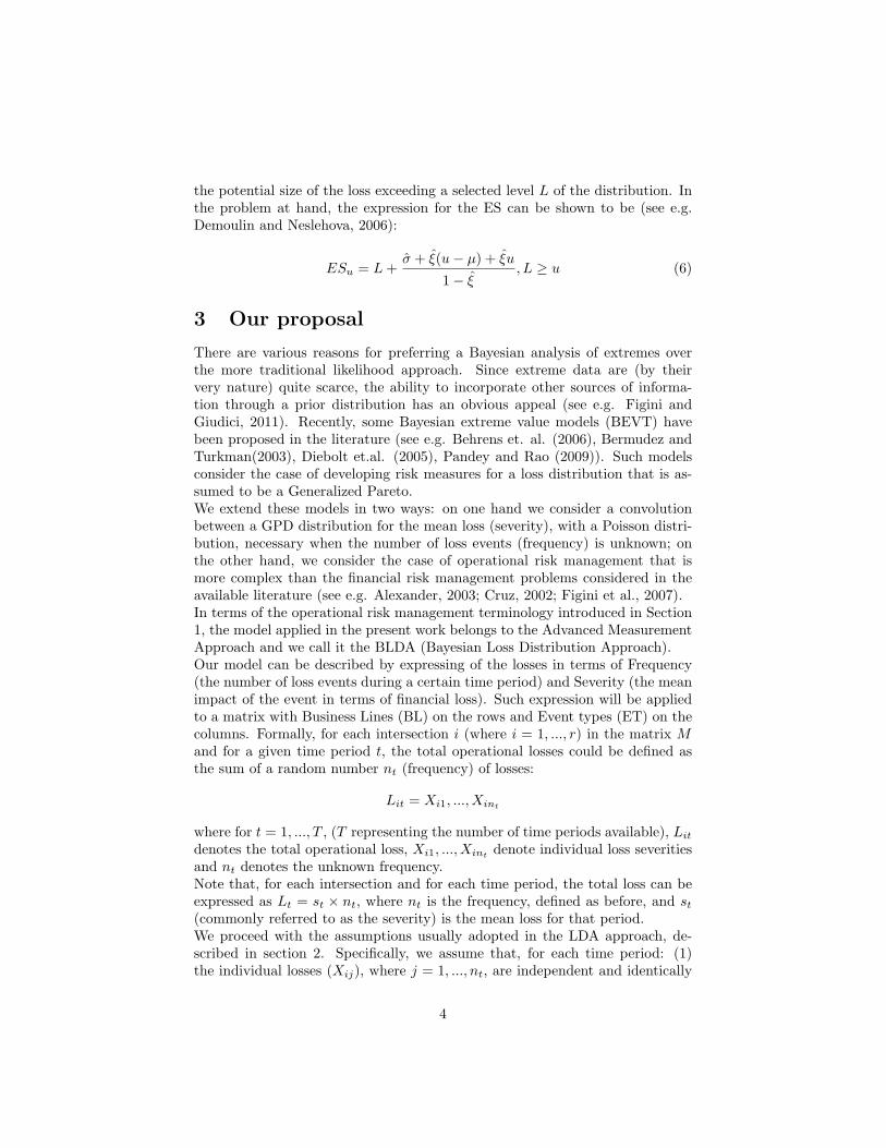
the potential size of the loss exceeding a selected level L of the distribution. Inthe problem at hand, the expression for the ES can be shown to be (see e.g.Demoulin and Neslehova, 2006):

ESu = L+σ̂ + ξ̂(u− µ) + ξ̂u

1− ξ̂, L ≥ u (6)

3 Our proposal

There are various reasons for preferring a Bayesian analysis of extremes overthe more traditional likelihood approach. Since extreme data are (by theirvery nature) quite scarce, the ability to incorporate other sources of informa-tion through a prior distribution has an obvious appeal (see e.g. Figini andGiudici, 2011). Recently, some Bayesian extreme value models (BEVT) havebeen proposed in the literature (see e.g. Behrens et. al. (2006), Bermudez andTurkman(2003), Diebolt et.al. (2005), Pandey and Rao (2009)). Such modelsconsider the case of developing risk measures for a loss distribution that is as-sumed to be a Generalized Pareto.We extend these models in two ways: on one hand we consider a convolutionbetween a GPD distribution for the mean loss (severity), with a Poisson distri-bution, necessary when the number of loss events (frequency) is unknown; onthe other hand, we consider the case of operational risk management that ismore complex than the financial risk management problems considered in theavailable literature (see e.g. Alexander, 2003; Cruz, 2002; Figini et al., 2007).In terms of the operational risk management terminology introduced in Section1, the model applied in the present work belongs to the Advanced MeasurementApproach and we call it the BLDA (Bayesian Loss Distribution Approach).Our model can be described by expressing of the losses in terms of Frequency(the number of loss events during a certain time period) and Severity (the meanimpact of the event in terms of financial loss). Such expression will be appliedto a matrix with Business Lines (BL) on the rows and Event types (ET) on thecolumns. Formally, for each intersection i (where i = 1, ..., r) in the matrix Mand for a given time period t, the total operational losses could be defined asthe sum of a random number nt (frequency) of losses:

Lit = Xi1, ..., Xint

where for t = 1, ..., T , (T representing the number of time periods available), Litdenotes the total operational loss, Xi1, ..., Xint

denote individual loss severitiesand nt denotes the unknown frequency.Note that, for each intersection and for each time period, the total loss can beexpressed as Lt = st × nt, where nt is the frequency, defined as before, and st(commonly referred to as the severity) is the mean loss for that period.We proceed with the assumptions usually adopted in the LDA approach, de-scribed in section 2. Specifically, we assume that, for each time period: (1)the individual losses (Xij), where j = 1, ..., nt, are independent and identically

4

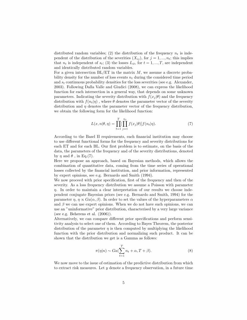
distributed random variables; (2) the distribution of the frequency nt is inde-pendent of the distribution of the severities (Xij), for j = 1, ..., nt; this impliesthat nt is independent of st; (3) the losses Lit, for t = 1, ..., T , are independentand identically distributed random variables.For a given intersection BL/ET in the matrix M , we assume a discrete proba-bility density for the number of loss events nt during the considered time periodand st continuous probability densities for the loss severities (see e.g. Alexander,2003). Following Dalla Valle and Giudici (2008), we can express the likelihoodfunction for each intersection in a general way, that depends on some unknownparameters. Indicating the severity distribution with f(xj |θ) and the frequencydistribution with f(nt|η) , where θ denotes the parameter vector of the severitydistribution and η denotes the parameter vector of the frequency distribution,we obtain the following form for the likelihood function:

L(x, n|θ, η) =T∏t=1

[nt∏j=1

f(xj |θ)]f(nt|η). (7)

According to the Basel II requirements, each financial institution may chooseto use different functional forms for the frequency and severity distributions foreach ET and for each BL. Our first problem is to estimate, on the basis of thedata, the parameters of the frequency and of the severity distributions, denotedby η and θ , in Eq.(7).Here we propose an approach, based on Bayesian methods, which allows thecombination of quantitative data, coming from the time series of operationallosses collected by the financial institution, and prior information, representedby expert opinions, see e.g. Bernardo and Smith (1994).We now proceed with prior specification, first of the frequency and then of theseverity. As a loss frequency distribution we assume a Poisson with parameterη. In order to maintain a clear interpretation of our results we choose inde-pendent conjugate Bayesian priors (see e.g. Bernardo and Smith, 1994) for theparameter η, η ∝ Ga(α, β). In order to set the values of the hyperparameters αand β we can use expert opinions. When we do not have such opinions, we canuse an ”uninformative” prior distribution, characterised by a very large variance(see e.g. Beherens et al. (2006)).Alternatively, we can compare different prior specifications and perform sensi-tivity analysis to select one of them. According to Bayes Theorem, the posteriordistribution of the parameter η is then computed by multiplying the likelihoodfunction with the prior distribution and normalizing such product. It can beshown that the distribution we get is a Gamma as follows:

π(η|n) ∼ Ga(T∑t=1

nt + α, T + β). (8)

We now move to the issue of estimation of the predictive distribution from whichto extract risk measures. Let y denote a frequency observation, in a future time

5

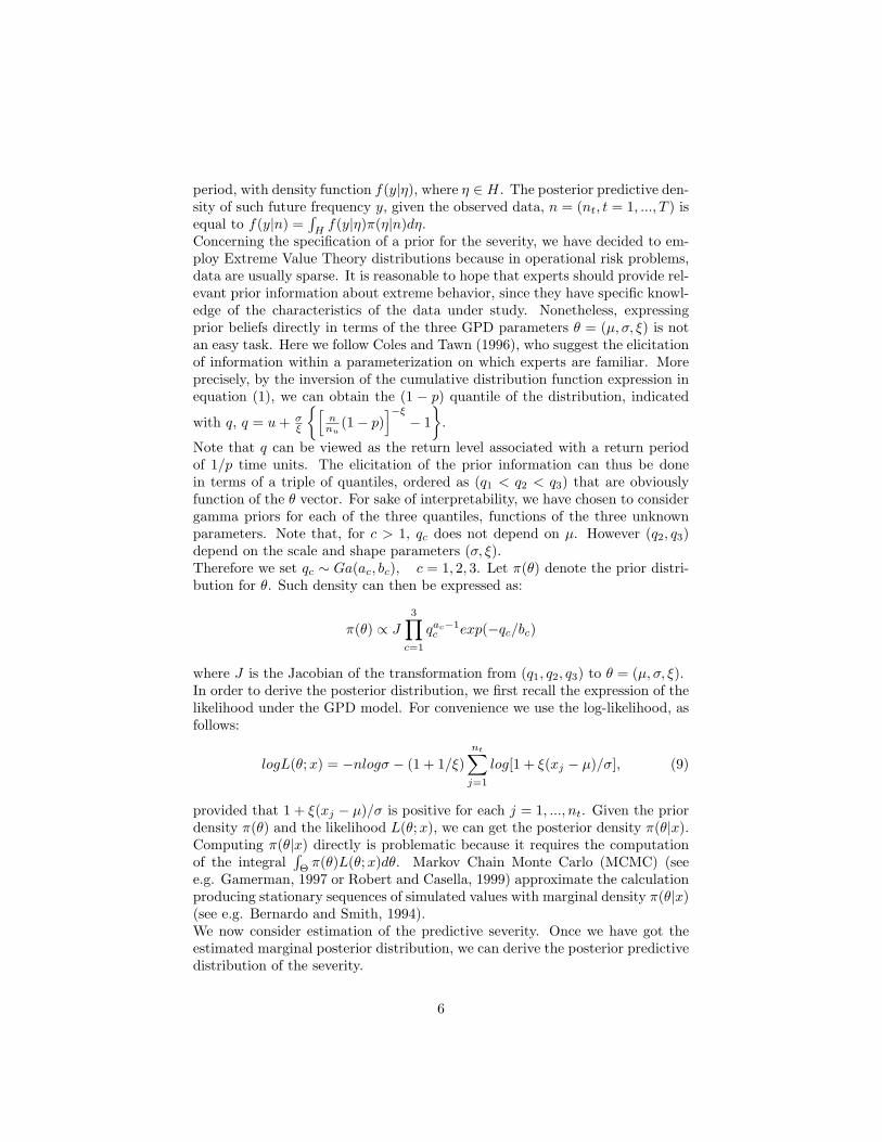
period, with density function f(y|η), where η ∈ H. The posterior predictive den-sity of such future frequency y, given the observed data, n = (nt, t = 1, ..., T ) isequal to f(y|n) =

∫Hf(y|η)π(η|n)dη.

Concerning the specification of a prior for the severity, we have decided to em-ploy Extreme Value Theory distributions because in operational risk problems,data are usually sparse. It is reasonable to hope that experts should provide rel-evant prior information about extreme behavior, since they have specific knowl-edge of the characteristics of the data under study. Nonetheless, expressingprior beliefs directly in terms of the three GPD parameters θ = (µ, σ, ξ) is notan easy task. Here we follow Coles and Tawn (1996), who suggest the elicitationof information within a parameterization on which experts are familiar. Moreprecisely, by the inversion of the cumulative distribution function expression inequation (1), we can obtain the (1 − p) quantile of the distribution, indicated

with q, q = u+ σξ

{[nnu

(1− p)]−ξ− 1}

.

Note that q can be viewed as the return level associated with a return periodof 1/p time units. The elicitation of the prior information can thus be donein terms of a triple of quantiles, ordered as (q1 < q2 < q3) that are obviouslyfunction of the θ vector. For sake of interpretability, we have chosen to considergamma priors for each of the three quantiles, functions of the three unknownparameters. Note that, for c > 1, qc does not depend on µ. However (q2, q3)depend on the scale and shape parameters (σ, ξ).Therefore we set qc ∼ Ga(ac, bc), c = 1, 2, 3. Let π(θ) denote the prior distri-bution for θ. Such density can then be expressed as:

π(θ) ∝ J3∏c=1

qac−1c exp(−qc/bc)

where J is the Jacobian of the transformation from (q1, q2, q3) to θ = (µ, σ, ξ).In order to derive the posterior distribution, we first recall the expression of thelikelihood under the GPD model. For convenience we use the log-likelihood, asfollows:

logL(θ;x) = −nlogσ − (1 + 1/ξ)nt∑j=1

log[1 + ξ(xj − µ)/σ], (9)

provided that 1 + ξ(xj − µ)/σ is positive for each j = 1, ..., nt. Given the priordensity π(θ) and the likelihood L(θ;x), we can get the posterior density π(θ|x).Computing π(θ|x) directly is problematic because it requires the computationof the integral

∫Θπ(θ)L(θ;x)dθ. Markov Chain Monte Carlo (MCMC) (see

e.g. Gamerman, 1997 or Robert and Casella, 1999) approximate the calculationproducing stationary sequences of simulated values with marginal density π(θ|x)(see e.g. Bernardo and Smith, 1994).We now consider estimation of the predictive severity. Once we have got theestimated marginal posterior distribution, we can derive the posterior predictivedistribution of the severity.

6

Let z denote a future observation of the severity with density function f(z|θ) ,where θ ∈ Θ. The posterior predictive density of z , given the observed data x,is f(z|x) =

∫Θf(z|θ)π(θ|x)dθ.

Using the MCMC approach, the predictive distribution can be estimated using1

n−b+1

∑ni=b P (Z ≤ z|θ(k)) , where n is the length of the chain and b is an

appropriately chosen burn-in parameter.In order to derive a measure at risk we need to merge the predictive severity withthe predictive frequency obtained before. This can be done by convoluting thepredictive frequency with the predictive severity via a Monte Carlo simulation(see e.g. Dalla Valle and Giudici 2008 and Gao et al. 2006, Kenett et al. 2010).Computationally this can be done along the following steps:Step1. For each time period to be predicted, generate n random observationsfrom the predictive frequency distribution;Step 2. For each period, generate a number of losses from the predictive severitydistribution equal to the corresponding frequency observation drawn in step 1(that is, if the simulated frequency of events for period k is nk, we simulate nkseverity losses from the predictive severity marginal distribution) .Step 3. For each period, sum the losses obtained in step 2, obtaining a lossobservation for the period, drawn from the convoluted marginal distribution asdescribed, thereby obtaining one loss observations for each period.Step 4. Using the loss observations obtained in step 3, estimate the predictiveloss distribution and obtain the V aR and ES, the risk measures that establishhow much capital is at risk.

4 Application

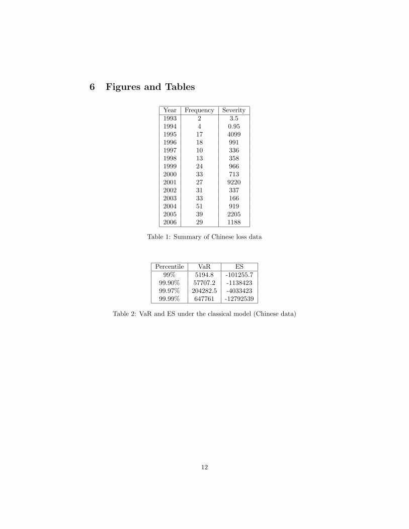
In this section we describe how our proposal works on two different sets of data.The first data set we use in our analysis contains the external operational lossesof Chinese commercial banks, ranging from 1993 to 2006. The number of lossdata collected is equal to 860. In this analysis we concentrate on 331 loss eventsextracted for a specific Business Line and a given Event Type. Table 1 reportsthe frequency and the severity (million yuan) for each year.

Table 1 about here

From the data in Table 1, the overall average yearly loss is equal to 1535.81million Yuan, the minimum is equal to 0.95 million Yuan and the maximum isequal to 9220.22 million Yuan.For the data at hand, we have first considered classical EVT models, as describedin Section 2. In order to select the threshold, and consequently estimate theparameters, we have employed the mean residual life plot and the thresholdchoice plot (see e.g. Coles, et. al. 1999). We have found that the thresholdcan be taken equal to 43. In correspondence to this settings, the frequency ofthe exceedances is equal to 60.45%, which suggests the employment of an EVTmodel. On the basis of the estimated parameters, under the EVT model, we canderive the combined distribution of frequency and severity via a Monte Carlo

7

simulation. Table 2 reports the VaR and the ES estimated under the classicalapproach.

Table 2 about here

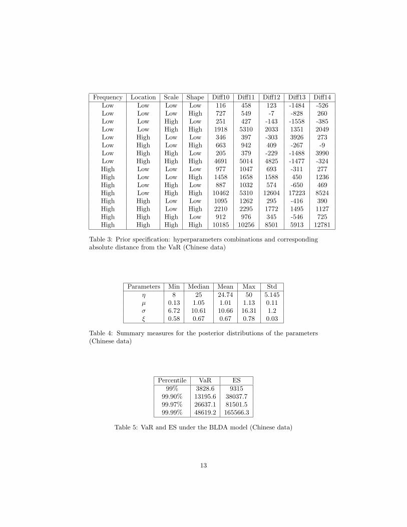
Since the estimated shape parameter of the GPD distribution is greater than 1(is equal to 1.1), in Table 2 we obtain that all expected shortfall become nega-tive. This means that the classical model is not adequate to obtain a coherentmeasure of risk.We move now to the application of our Bayesian model, using 50000 iterationsin the MCMC algortihm. First we should choose the right priors for the distri-bution. Since we have no actual expert opinion, we follow a sensitivity analysisapproach, specifing a number of alternative priors under different combinationsof hyperparameters settings. In particular for the frequency parameter priordistribution, we consider two prior settings: low=(1,20) and high=(40,1). Onthe other hand, for all of the three severity quantiles prior distributions we con-sider two prior specifications: low=(1,1) and high=(30,30). This leads to a totalof 16 alternative prior specifications that will be compared in terms of backtest-ing: choosing the prior that leads to the smallest difference in absolute valuebetween the VaR and the observed losses. For sake of precision we have runthe backtesting using the first 9 years as a training period and the subsequent5 years as test period on a moving window basis. Table 3 reports the results ofthe sensitivity analysis: for each specified prior we report the loss exceedancesfor periods 10 trough 14.

Table 3 about here

From Table 3 note that the HLLH combination is the best one: with it the VaRcovers all the real total losses and the mean difference between the VaR and theobserved losses is the smallest one. Table 4 shows the posterior summaries forall parameters under the chosen prior specification.

Table 4 about here

From Table 4, the posterior mean frequency is equal to 24.74 and the median isequal to 25. The results seem coherent with the observed sample mean, whichis equal to 23.64. Using the results described before, we are thus able to obtainthe predictive distribution for the severity and to combine it with the predictivefrequency distribution via Monte Carlo simulation, as explained in Section 3.The combined distribution allows us to derive the risk measures, as in Table 5.

Table 5 about here

We can compare the results in Table 5 with those in Table 2, relative to theclassical model. Note that, using our BLDA model, we can obtain a remarkablereduction in terms of VaR (always lower in the BLDA case) and, therefore, alower capital charge.The second data set we use in our analysis contains one specific business line(retail banking) and a given event type (external fraud) of the internal database

8

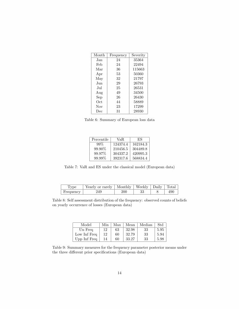
of operational losses of an anonymous European bank, ranging from October2006 to December 2010. The number of loss data collected is equal to 1855. Inorder to use the self-assessment data, in this analysis we concentrate on the lossof 2009, composed of 396 loss events. The overall average month loss is equalto 38777.41 Euro, while the minimum and the maximum are equal to 17298.68and 115662.5 Euro respectively. Considering retail banking and external fraudas business line and event type, Table 6 reports for each month the frequencyand severity distributions.

Table 6 about here

As we can observe from Table 6, external fraud events are generally stable acrossthe time period considered, except for April and August, while the average forthe severity shows an increasing in March and October.We now apply a classical model. In order to estimate the threshold and conse-quently the scale and the shape parameters, we have employed the mean residuallife plot and the threshold choice plot (see e.g. Coles et al. 1999). We havefound that the threshold can be fixed equal to 1230. In correspondence to thissetting, the frequency of the exceedances is equal to 18.45%, which confirms theemployment of an EVT model. In the classical perspective, on the basis of theestimated parameters, we can compute the combined distribution of frequencyand severity via a Monte Carlo simulation. Table 7 reports the VaR and the ESestimated for the integrated distribution at hand using the classical model.

Table 7 about here

From Table 7, note that the ES is positive, differently from what happened inthe chinese data.In order to build our Bayesian model, we now construct a prior distribution forthe frequency using qualitative data provided by the bank. The informationcontained in the qualitative data is based on prior opinions obtained from a selfassessment questionnaire submitted to the process owners of the bank.In order to evaluate the impact of actual prior opinions we first specify an un-informative prior without self-assessment characterised by a very high variance.Using such prior, the posterior mean is equal to 32.98 and the posterior me-dian is equal to 33. This result seems coherent with the observed sample mean,which is equal to 33. The number of iterations of the MCMC algorithm wastaken equal to 35000.We now consider an informative prior that uses self assessment opinions. Thesummary of such opinions, on frequencies, are shown in Table 8.

Table 8 about here

We have decided to use an approximate confidence interval for binomial propor-tions to specify the prior hyperparameters, for example under a 95% confidencelevel. Under this framework we get two reference prior distributions: one thatwe call lower informative, with hyperparameters set at the lower bound of theconfidence interval, and one, conversely, upper informative. More precisely, the

9

lower informative prior turns out to be Gamma (7.3748, 0.2951) and the upperinformative prior Gamma (19.5329, 0.4803). Table 9 shows the summaries ofthe posterior distribution of the frequency parameter under, respectively, anuninformative prior, a lower informative and an upper informative priors.

Table 9 about here

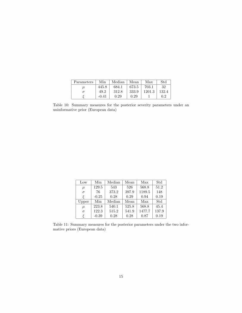
Table 9 shows that the insertion of a self-assessment prior in the model doesnot change substantially the posterior estimates obtained with an uninformativeprior.We now move to the task of specifying prior distribution for the severity. Wefirst consider uninformative Gamma prior characterised by a large variance. Ta-ble 10 reports summary measures for the corresponding posterior distribution.In the MCMC algorithm the number of iterations is equal to 35000.

Table 10 about here

We now consider an informative prior, based on self-assessment data, for theseverity distribution. Following a procedure similar to what exposed for thefrequency prior, as opinions on severity are expressed on an ordinal scale asfrequency ones, we get lower informative priors for the quantile parameters asGamma (13.5540, 91.7646), Gamma (0.1982, 26486.183) and Gamma (0.1532,14396.1), upper informative priors as Gamma (35.899, 56.386), Gamma (0.525,16274.64) and Gamma (0.406, 8845.817). Table 11 shows the posterior distri-bution summaries.

Table 11 about here

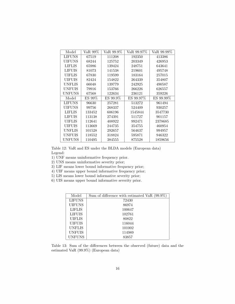
Using the results described before, we are thus able to obtain the predictivedistribution for the severity and combine it with the predictive frequency dis-tribution via Monte Carlo simulation, as explained in Section 3. The combineddistribution allows us to derive the risk measures, as shown in Table 12.

Table 12 about here

We can compare the VaRs estimated in the above table, based on the 2009monthly data, with the actual losses occurred in the year 2010. Concerning the99.9% VaR, which is the most used reference in operational risk management,we have obtained that all VaRs, except that calculated with the LIFUNS modelcover all actual 2010 losses.For all model we also derived the Expected Shortfall. In order to chose amongall remaining models we have computed in Table 13 the sum of the differencesbetween each VaR and all 2010 observed losses.

Table 13 about here

From Table 13 the best models, in terms of minimisation of the differences withthe VaR and the observed losses are : LIFUNS, UIFLIS, UNFUNS, UIFUNS.

10

However, LIFUNS can be excluded as the corresponding VaR does not coverall losses. Among the remaining three models, the model with the lowest Ex-pected Shortfall is UIFUNS which therefore will be chosen. UIFLIS has a highExpected Shortfall and, therefore, will also be excluded, being incoherent. Inconclusion, we support choosing the UNFUNS or the UIFUNS model, the for-mer being totally uninformative and the second partly informative.We remark that the latter has indeed a cover expected shortfall. In order tocompare our BLDA model with the classical one, we can use the VaR, as re-ported in Table 7 and Table 13. Note that, using the BLDA model, we canobtain a remarkable reduction in terms of VaR (always lower, especially withself-assessment prior, in the BLDA case) and, therefore, a lower capital charge.

5 Concluding remarks

The main purpose of this paper is to introduce a new methodology for esti-mating the loss distributions in operational risk management in a predictiveframework. Our main outcome is that the application of Bayesian methodologycauses a reduction of value at risks and, therefore, of the capital charge com-pared to the classical extreme value analysis method. This is a very importantresult in terms of money saved by the financial institution adopting this ap-proach.We also remark that the two examined cases are based on very different, yetcomplementary, datasets: the Chinese data are basically uninformative data,with dynamic nature; the European data considers a short time horizon andinclude self-assessment data, and consequently, the BLDA model is based on in-formative data to derive the prior knowledge. In both cases, our BLDA shows aloss reduction compared with the classical extreme model and therefore a greatreduction in terms of capital charged.Our results finally show that using a self-assessment data to specify an infor-mative prior, leads to results that are little better than with an uninformativeprior model, so it is helpful that banks collect and analyse self-assessment expertopinions.An interesting development of our research could be the extension to other risktypes, and a multivariate analysis of all event type/business lines combinations,although this latter would involve multivariate self-assesment (see e.g. Bonafedeand Giudici, 2007).

11

6 Figures and Tables

Year Frequency Severity1993 2 3.51994 4 0.951995 17 40991996 18 9911997 10 3361998 13 3581999 24 9662000 33 7132001 27 92202002 31 3372003 33 1662004 51 9192005 39 22052006 29 1188

Table 1: Summary of Chinese loss data

Percentile VaR ES99% 5194.8 -101255.7

99.90% 57707.2 -113842399.97% 204282.5 -403342399.99% 647761 -12792539

Table 2: VaR and ES under the classical model (Chinese data)

12

Frequency Location Scale Shape Diff10 Diff11 Diff12 Diff13 Diff14Low Low Low Low 116 458 123 -1484 -526Low Low Low High 727 549 -7 -828 260Low Low High Low 251 427 -143 -1558 -385Low Low High High 1918 5310 2033 1351 2049Low High Low Low 346 397 -303 3926 273Low High Low High 663 942 409 -267 -9Low High High Low 205 379 -229 -1488 3990Low High High High 4691 5014 4825 -1477 -324High Low Low Low 977 1047 693 -311 277High Low Low High 1458 1658 1588 450 1236High Low High Low 887 1032 574 -650 469High Low High High 10462 5310 12604 17223 8524High High Low Low 1095 1262 295 -416 390High High Low High 2210 2295 1772 1495 1127High High High Low 912 976 345 -546 725High High High High 10185 10256 8501 5913 12781

Table 3: Prior specification: hyperparameters combinations and correspondingabsolute distance from the VaR (Chinese data)

Parameters Min Median Mean Max Stdη 8 25 24.74 50 5.145µ 0.13 1.05 1.01 1.13 0.11σ 6.72 10.61 10.66 16.31 1.2ξ 0.58 0.67 0.67 0.78 0.03

Table 4: Summary measures for the posterior distributions of the parameters(Chinese data)

Percentile VaR ES99% 3828.6 9315

99.90% 13195.6 38037.799.97% 26637.1 81501.599.99% 48619.2 165566.3

Table 5: VaR and ES under the BLDA model (Chinese data)

13

Month Frequency SeverityJan 24 35364Feb 24 22494Mar 36 115663Apr 53 50360May 32 21797Jun 29 26793Jul 25 26531Aug 49 34500Sep 26 26430Oct 44 58889Nov 23 17299Dec 31 28930

Table 6: Summary of European loss data

Percentile VaR ES99% 124374.4 162184.3

99.90% 210456.5 304489.899.97% 304337.2 420995.399.99% 392317.6 568834.4

Table 7: VaR and ES under the classical model (European data)

Type Yearly or rarely Monthly Weekly Daily TotalFrequency 249 200 33 8 490

Table 8: Self assessment distribution of the frequency: observed counts of beliefson yearly occurrence of losses (European data)

Model Min Max Mean Median StdUn Freq 12 63 32.98 33 5.95

Low Inf Freq 12 60 32.79 33 5.94Upp Inf Freq 14 60 33.27 33 5.98

Table 9: Summary measures for the frequency parameter posterior means underthe three different prior specifications (European data)

14

Parameters Min Median Mean Max Stdµ 445.8 684.1 673.5 703.1 32σ 49.2 312.8 333.9 1201.3 132.4ξ -0.41 0.29 0.29 1 0.2

Table 10: Summary measures for the posterior severity parameters under anuninformative prior (European data)

Low Min Median Mean Max Stdµ 129.5 543 526 568.8 51.2σ 76 373.2 397.9 1189.5 148ξ -0.25 0.28 0.29 0.94 0.19

Upper Min Median Mean Max Stdµ 223.8 540.1 525.8 568.8 45.4σ 122.3 515.2 541.9 1477.7 137.9ξ -0.39 0.28 0.28 0.87 0.19

Table 11: Summary measures for the posterior parameters under the two infor-mative priors (European data)

15

Model VaR 99% VaR 99.9% VaR 99.97% VaR 99.99%LIFUNS 67519 111208 192350 413386UIFUNS 68244 125752 203349 426953LIFLIS 65986 139424 248751 643641LIFUIS 81073 141538 219601 495748UIFLIS 67830 119599 183164 257015UIFUIS 82424 154822 264339 354807UNFLIS 66048 139779 242925 490587UNFUIS 79916 153766 266226 626557UNFUNS 67568 122634 236121 359226

Model ES 99% ES 99.9% ES 99.97% ES 99.99%LIFUNS 96630 257281 513272 961494UIFUNS 99756 268337 524409 930257LIFLIS 133452 606196 1545844 3547730LIFUIS 113138 274391 511727 901157UIFLIS 112641 408922 992471 2378685UIFUIS 113669 244735 354755 460954UNFLIS 101528 292657 564637 994957UNFUIS 118552 318824 595871 946322UNFUNS 110495 384555 875528 1859656

Table 12: VaR and ES under the BLDA models (European data)Legend:1) UNF means uninformative frequency prior.2) UNS means uninformative severity prior;3) LIF means lower bound informative frequency prior;4) UIF means upper bound informative frequency prior;5) LIS means lower bound informative severity prior;6) UIS means upper bound informative severity prior.

Model Sum of difference with estimated VaR (99.9%)LIFUNS 72430UIFUNS 86974LIFLIS 100647LIFUIS 102761UIFLIS 80822UIFUIS 116044UNFLIS 101002UNFUIS 114989UNFUNS 83857

Table 13: Sum of the differences between the observed (future) data and theestimated VaR (99.9%) (European data)

16

References

1. Acerbi, C., Tasche, D., 2002 On the coherence of expected shortfall. J.Banking Finance 26, 14871503.

2. Alexander, C., 2003 Operational Risk. Regulation, Analysis and manage-ment. In: Alexander, C. (Ed.), Financial Times Prentice Hall, London,pp. 130-170.

3. Artzner, P., Delbaen, F., Eber, J., Heath, D., 1999 Coherent measures ofrisk. Math. Finance 9 (3), 203228.

4. Balkema, A.A de Haan L., 1974 Residual life time at great age. Annals ofProbability 2, 792804.

5. Behrens, Cibele N., Hedibert F. Lopes, Dani Gamerman, 2006 Bayesiananalysis of extreme events with threshold estimation. Statistical Modelling6, 251263.

6. Bernardo, J.M., Smith, A.F.M., 1994 Bayesian Theory.Wiley, Chichester.

7. Bermudez P. de Zea, M.A. Amaral Turkman, 2003 Bayesian approach toparameter estimation of the generalized Pareto distribution. Sociedad deEstadistica e Investigacion Operation. Test 12(1), 259-277.

8. Bilotta A., Giudici P. 2004 Modelling operational losses: a bayesian ap-proach. Quality and Reliability Engineeering International, 20, pp. 407-417.

9. Bonafede E., P. Giudici 2007 Bayesian networks for enterprise risk assess-ment. Physica A, 382, pp 22-28

10. Coles SG, Tawn JA, 1996 A Bayesian analysis of extreme rainfall data.Applied Statistics 45,463-78.

11. Coles, S. J Heffernan and J. Tawn, 1999 Dependence measures for extremevalue analyses. Extremes 2(4), 339-365.

12. Cruz, M. G. 2002 Modeling, Measuring and Headging Operational Risk.John Wiley Sons, New York, Chichester, pp.101-118.

13. Dalla Valle L., P. Giudici, 2008 A Bayesian approach to estimate themarginal loss distributions in operational risk management. Computa-tional Statistics Data Analysis 52, 3107-3127.

14. Demoulin V.C., E. P. Neslehova, 2006 Quantitative models for OperationalRisk: Extremes, Dependence and Aggregation. Banking Finance 30,2635-2658.

17

15. Diebolt J., Mhamed-Ali El-Aroui, Myriam Garrido and Stphane Girard,2005. Quasi-conjugate Bayes estimates for GPD parameters and applica-tion to heavy tails modelling. Extremes 8, 57-78.

16. Figini S., Giudici P. 2011 Statistical merging of rating models, to appearin Journal of the operational research society.

17. Figini, S., Giudici P. and Uberti, P. 2010 A threshold based approach tomerge data in financial risk management, to appear in Journal of AppliedStatistics.

18. Figini, S., Giudici, P., Uberti, P. e Sanyal, A. 2007 A statistical methodto optimize the combination of internal and external data in operationalrisk measurement, in Journal of Operational Risk, Vol 2. N.4, pp. 69-78.

19. Figini, S., Kenett R.S. and Salini S. 2010 Optimal Scaling for Risk Assess-ment: Merging of Operational and Financial Data, to appear in Qualityand Reliability Engineering International, DOI: 10.1002/qre.1158.

20. Gamerman, D., 1997 Markov Chain Monte Carlo: Stochastic Simulationfor Bayesian Inference. Chapman Hall, London.

21. Gao L., Lee J., Chen J. and Xu, W. 2006 Assessment the Operational Riskfor Chinese Commercial Banks?in V.N. Alexandrov et al. (Eds.): ICCS,Part IV, LNCS 3994, pp. 501 508.

22. Gao L. and Lee, J. 2009 The influence of IPO to the operational risk ofChinese commercial banks. Springer House?Cutting-edge research topicson multiple criteria decision making,486-492.

23. Himanshu P., Arun Kumar Rao, 2009 Bayesian estimation of the shapeparameter of a Generalized Pareto Distribution under asymmetric func-tions. Mathematics and Statistics 38(1):69-83.

24. Kenett, R.S. and Tapiero, C., 2010 Quality, Risk and the Taleb Quadrants,Risk and Decision Analysis, in press.

25. Pandey H., and Rao K. 2009 Bayesian estimation of the shape parameterof a Generalized Pareto Distribution under asymmetric functions. Math-ematics and Statistics 38(1):69-83.

26. Pickands J., 1975 Statistical inference using extreme order statistics, An-nals of Statistics 3, 119-131.

27. Robert, C.P., Casella, G., 1999 Monte Carlo Statistical Methods. Springer,NewYork.

28. Yamai, Y., Yoshiba, T., 2002 Comparative analyses of expected shortfalland value-at-risk: their validity under market stress. Monetary and Econ.Stud. 181-238.

18

QUADERNI DEL DIPARTIMENTO DI ECONOMIA, STATISTICA E DIRITTO n. 1/2011 Paolo Giudici, Emanuela Raffinetti, A Gini concentration quality measure for

ordinal variables, Serie Statistica. n. 2/2011 Silvia Figini, Lijun Gao, Paolo Giudici, Bayesian efficient capital at risk estimation,

Serie Statistica.

COLLANE PRECEDENTI QUADERNI DEL DIPARTIMENTO DI ECONOMIA PUBBLICA E TERRITORIALE n. 1/2010 Silvio Beretta, Variabili finanziarie ed economia globale in tempo di crisi n. 2/2010 Silvio Beretta, Renata Targetti Lenti, L'India nel processo di integrazione internazionale.

Dal primo al secondo unbundling e la posizione dell'Italia n. 3/2010 Margarita Olivera, Challenges to Regional Integration in Latin America n. 4/2010 Italo Magnani, Un economista liberale guarda alla economia dell'ambiente: impressioni e

riflessioni n. 5/2010 Italo Magnani, A cinquant’anni dalla scomparsa di Benvenuto Griziotti: Riflessioni n. 6/2010 Luca Mantovan, Class-bias in Technology Adoption: Stagnation and Transformation of

Subsistence Agriculture in the Ethiopian Northern Highlands n. 7/2010 Marco Missaglia, Giovanni Valensisi, A trade-focused, post-Keynesian CGE model for

Palestine n. 8/2010 Giovanni Valensisi, Marco Missaglia, Reappraising the World Bank CGE model on

Palestine: macroeconomic and financial issues n. 1/2009 Giorgio Panella, Andrea Zatti, Fiorenza Carraro, Market Based Instruments for Energy

Sustainability n. 1/2008 Italo Magnani, Il pubblico e il privato nella economia della città n. 2/2008 Italo Magnani, Note a margine di una recente opera sull'indirizzo sociologico della scienza

delle finanze italiana n. 3/2008 Italo Magnani, La riforma sociale nella formazione di Nitti economista n. 4/2008 Marisa Bottiroli Civardi, Renata Targetti Lenti and Rosaria Vega Pansini, Multiplier

Decomposition, Poverty and Inequality in Income Distribution in a SAM Framework: The Vietnamese Case

n. 5/2008 Luca Mantovan, A Study on Rural Subsistence in the Ethiopian Northern Highlands [per i Quaderni precedenti si rinvia a http://www-5.unipv.it/webdesed/ept/quaderni.php ] QUADERNI DI RICERCA DEL DIPARTIMENTO DI STATISTICA ED ECONOMIA APPLICATE

“L. LENTI” Carla Ge Rondi, L'après mariage en Italie au début du XXIe siècle (2005, n. 27) Carla Ge Rondi, Casalinga: popolazione attiva senza retribuzione (2005, n. 25) Bruno Scarpa, David Dunson, Bayesian Methods for Searching for Optimal Rules for Timing Intercourse to

Achieve Pregnancy (2005, n. 24) Bruno Scarpa, Lo stress in azienda. Modelli di analisi di un'indagine per l'identificazione delle cause di

stress (2004, n. 23) Bruno Scarpa, La Customer Satisfaction per un'azienda di servizi informatici. Impostazione e analisi di

un'indagine via web (2004, n. 22) [per i Quaderni precedenti si rinvia a http://www-5.unipv.it/webdesed/lenti/quaderni.php ] OSSERVATORIO DEI CONTRATTI DELLA P.A. [Si rinvia a http://www.contratti-appalti.it/ ]