Embed Size (px)
Citation preview

TA
Sc
MB
Da
ScAuUNhtt
ISSIS
he UnivAustralian
chool of Ec
Mutual Fuenchma
aniel Bunc
chool of Econustralian SchNSW Sydneytp://www.eco
SN 1837-103BN 978-0-73
ersity ofn Schoo
conomics D
und Stylarks and
cic, Jon E. E
nomics ool of Busine
y NSW 2052 onomics.unsw
35334-2911-8
f New Sool of Bus
Discussion
e, Chara Activity
Eggins, an
essAustralia
w.edu.au
outh Wainess
Paper: 20
acteristicy Measu
d Robert J
ales
10/12
c-Matchres: A N
J. Hill
hed PerfoNew App
ormanceproach
e

MUTUAL FUND STYLE, CHARACTERISTIC-MATCHED
PERFORMANCE BENCHMARKS AND ACTIVITY MEASURES:
A NEW APPROACH∗
DANIEL BUNCIC
Institute of Mathematics & StatisticsUniversity of St. Gallen
Switzerland
JON E. EGGINS
Russell Investment Group909 A Street, Tacoma
WA98402, USA
ROBERT J. HILL‡
School of EconomicsUniversity of Graz
Austria
June 22, 2010
Abstract
We propose a new approach for measuring mutual fund style and constructingcharacteristic-matched performance benchmarks that requires only portfolio holdingsand two reference portfolios in each style dimension. The characteristic-matched per-formance benchmark literature typically follows a bottom-up approach by first match-ing individual stocks with benchmarks and then obtaining a portfolio’s excess returnas a weighted average of the excess returns on each of its constituent stocks. Ourapproach is fundamentally different in that it matches portfolios and benchmarks di-rectly. We illustrate our approach using portfolio holdings of 1183 fund managersover the period 2002-2009. We characterize the cross-section of fund manager stylesand show how average style changes over time. The tracking error volatilities of ourcharacteristic-matched benchmarks compare favorably with those of existing meth-ods. Using our benchmarks we explore the link between activity and performance.
Keywords: Performance Measurement; Tailored Benchmark; Characteristic Matching;Size Profile; Growth Profile; Activity; Excess ReturnJEL Classification: C43, G11, G23.
∗The views expressed in this paper are those of the authors and do not necessarily reflect those of the RussellInvestment Group. The research of Hill, formerly of University of New South Wales in Sydney, Australia,was partially supported by the Australian Research Council (grant DP0666798). Hill is visiting UNSW inthe second half of 2010.‡Corresponding Author.
1

1. Introduction
The measurement of style and performance of managed portfolios is of fundamental im-
portance to the investment industry. Accurate measurement of style allows investors to
obtain their desired exposures to particular investment styles.1 It also is a prerequisite to
reliable performance measurement, since the performance of a fund manager should be
judged relative to an appropriate style benchmark. For example, a manager focusing on
small-cap stocks should be evaluated against a small-cap benchmark, while a manager
that follows a growth investing style should have performance compared to a growth
benchmark.
Matching of funds and benchmarks based on declared style (as is done for example by
Morningstar) can be problematic since declared style does not necessarily match observed
style (see Sharpe, 1988, 1992, Carhart, 1997, Brown and Goetzmann, 1997, diBartolomeo
and Witkowski, 1997, Chan, Chen and Lakonishok, 2002).
Two main approaches have been used in the literature for ensuring that funds are
matched with appropriate benchmarks. The first approach is regression based using past
returns. Its point of departure is the capital asset pricing model (CAPM). A tailored bench-
mark is obtained by taking a linear combination of the risk-free and market benchmark
rate of returns, with the weight for each fund determined by its value of beta. The dif-
ference between a portfolio’s actual performance and its tailored benchmark is referred
to as Jensen’s alpha (see Jensen, 1967, 1969). Jensen’s alpha is calculated as the intercept
of an excess return regression. This basic model can be extended by including additional
1A pension plan, for example, has to consider the coherence of its overall strategy. It may wish to followa blend strategy, and try and achieve this goal by giving half the managers value mandates and the otherhalf growth mandates. To achieve the overall desired strategy, it is important to monitor the managers’observed style relative to their assigned mandates. Alternatively, a firm may hope that by hiring a numberof managers it is diversifying its overall portfolio. In this case, the objective is to ensure that the styles of themanagers are sufficiently diversified. The more accurately a firm can measure what its managers are doing,the better able it will be to achieve its desired overall strategy.
2

non-CAPM factors such as size, valuation and momentum (see Fama and French, 1992,
1996, and Carhart, 1997). Sharpe (1988, 1992) proposes an alternative regression model
based on asset class factors. He uses this to determine the effective mix of a portfolio in
terms of the underlying asset classes. A tailored benchmark can then be constructed as a
weighted average of these asset class benchmarks, with the weights determined from the
regression equation.
Regression-based methods only require data on fund performance, and factors such
as size and the price-to-book ratio. To estimate the regression equation, however, a fairly
long time series of observations is required. This can be problematic since the style of a
fund and the factor parameters could change over time.
The second approach requires portfolio holdings data, but has the advantage that it re-
quires only short time horizons. Expositors of this approach include Daniel, Grinblatt, Tit-
man and Wermers (1997), henceforth DGTW, Chan, Chen and Lakonishok (2002), hence-
forth CCL, and Chan, Dimmock and Lakonishok (2009), henceforth CDL, (see also Kothari
and Warner, 2001). These authors match characteristics at the level of individual stocks.
Stocks are first sorted in each style dimension, and then divided into quintile blocks. In
two dimensions (say size and value-growth), this generates a total of 25 blocks. CDL
show that the resulting benchmarks can be quite sensitive to the way these sorts are done
(e.g., whether or not growth is sorted independently of size). DGTW construct a market-
cap-weighted benchmark portfolio from each block, while CCL construct equal-weighted
portfolios from each block. CDL also show that the choice between market-cap and equal
weighting can significantly affect the results. Each stock in a portfolio is matched with the
benchmark portfolio with the most similar style characteristics. The excess return on each
stock is measured by the difference between its return and its benchmark’s return. An
overall performance benchmark for a portfolio is then obtained by taking the weighted
mean of these excess returns, where each stock is weighted by its dollar share of the port-
3

folio. Each fund, therefore, has its own distinct performance benchmark.
In this paper we develop a new variant on this second approach that differs from
DGTW, CCL and CDL in a number of respects. First, our matching of characteristics
is done at the level of portfolios, rather than at the level of individual stocks. Second, our
benchmarks are defined in a continuous style space, and hence we achieve a direct match
between portfolios and benchmarks. By contrast, the DGTW-CCL-CDL approach matches
stocks with one of a finite number of benchmark portfolios, and hence these matches are
more approximate. Finally, our method is computationally simple and intuitive. For each
dimension our method requires only two reference portfolios, which can often be taken
off the shelf from index providers. For example, the Russell 3000 Value and Russell 3000
Growth indices could be used in the value-growth dimension.2
Our approach begins by determining a portfolio’s location in style space. We propose
a new formula for doing this which can be applied in each dimension.3 Our new style
measures are of interest in their own right. However, we then show how they can be used
to construct performance benchmarks that are tailored specifically to the style of each
fund in each style dimension. Our approach has further extensions. First, it can be used
to disentangle the effects of different style dimensions on performance. For example, we
can assess the impact of changes in size holding the value-growth style fixed. Second, it
generates new measures of activity of funds relative to their tailored benchmarks.4
We apply our methodology to a US mutual fund data set consisting of 1183 manager
portfolios over the period 2002-2009. In the size and value-growth style dimensions, we
2By assets benchmarked, Russell’s style indices account for more than 98 percent of market share forUS equity growth and value oriented products (see Russell Investments, 2008). For illustrative purposestherefore we construct our off-the-shelf portfolios from Russell indices.
3CCL also propose a method for locating portfolios in style space. However, their style-space is notcontinuous. Also, they do not use it to construct performance benchmarks.
4There is some ambiguity in the literature regarding the use of the term ’activity’. It is sometimes used torefer to turnover. Here, however, by ‘activity’ we mean departures from passive tracking of a benchmark.
4

illustrate the cross-section diversity of styles across managers and the gradual shift in
style towards growth stocks from 2002 to 2009. We also show how the size profiles of the
Russell 1000 Growth and Russell 1000 Value indices, and the growth profile of the Russell
1000 and index, change over time. We then compute tracking error volatilities for a few
variants on our basic characteristic-matched benchmarking method and for the preferred
method in CDL. At least some of our benchmarks are competitive in terms of tracking
error volatility with CDL’s preferred benchmark. Using our new benchmarks, we also
explore the link between activity and performance. Our main findings are summarized in
the conclusion.
2. Style Profiles and One-Dimensional Tailored Performance Benchmarks
2.1. Style profiles
Portfolios can be classified by style in a number of dimensions. Two of the most commonly
considered styles are size and value-growth. We define a style profile P(w) as a function
that maps an N-dimensional portfolio w into one style dimension to generate an ordinal
ranking of portfolios according to that particular style. For example, suppose P(w1) >
P(w2). It follows that in this style dimension, portfolio w1 attains a higher score than
portfolio w2.
Let lg and sm denote two reference portfolios in a given style dimension, such that
P(sm) < P(lg) (i.e., lg and sm are abbreviations for reference large and small portfolios in
this dimension). For example, in the size dimension lg could be the Russell 3000 portfolio,
and sm an equally weighted variant on the Russell 3000 portfolio.5 In the value-growth
dimension, lg could be the Russell 3000 Growth portfolio, and sm the Russell 3000 Value
portfolio, etc.
5Henceforth although we will frequently refer to the Russell 3000 Equal-Weighted index, it should benoted that the Russell Investment Group does not actually publish such an index. However, this index andits underlying portfolio can easily be constructed.
5
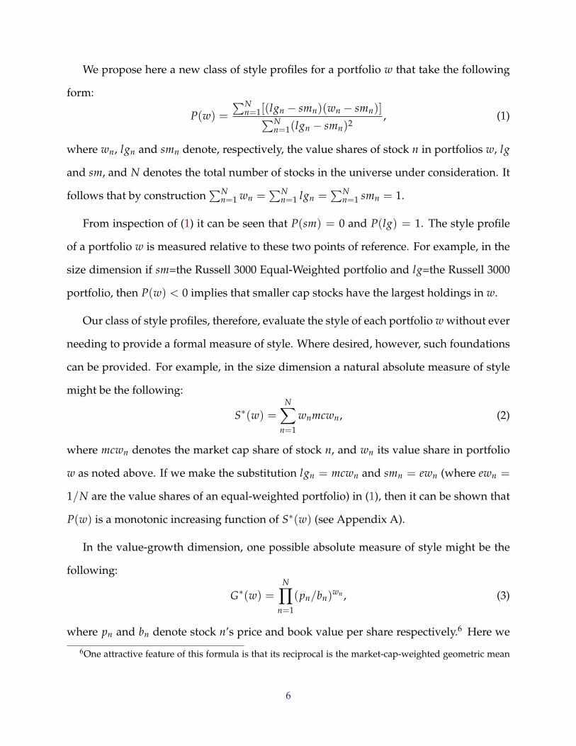
We propose here a new class of style profiles for a portfolio w that take the following
form:
P(w) =
∑Nn=1[(lgn − smn)(wn − smn)]∑N
n=1(lgn − smn)2, (1)
where wn, lgn and smn denote, respectively, the value shares of stock n in portfolios w, lg
and sm, and N denotes the total number of stocks in the universe under consideration. It
follows that by construction∑N
n=1 wn =∑N
n=1 lgn =∑N
n=1 smn = 1.
From inspection of (1) it can be seen that P(sm) = 0 and P(lg) = 1. The style profile
of a portfolio w is measured relative to these two points of reference. For example, in the
size dimension if sm=the Russell 3000 Equal-Weighted portfolio and lg=the Russell 3000
portfolio, then P(w) < 0 implies that smaller cap stocks have the largest holdings in w.
Our class of style profiles, therefore, evaluate the style of each portfolio w without ever
needing to provide a formal measure of style. Where desired, however, such foundations
can be provided. For example, in the size dimension a natural absolute measure of style
might be the following:
S∗(w) =N∑
n=1
wnmcwn, (2)
where mcwn denotes the market cap share of stock n, and wn its value share in portfolio
w as noted above. If we make the substitution lgn = mcwn and smn = ewn (where ewn =
1/N are the value shares of an equal-weighted portfolio) in (1), then it can be shown that
P(w) is a monotonic increasing function of S∗(w) (see Appendix A).
In the value-growth dimension, one possible absolute measure of style might be the
following:
G∗(w) =N∏
n=1
(pn/bn)wn , (3)
where pn and bn denote stock n’s price and book value per share respectively.6 Here we
6One attractive feature of this formula is that its reciprocal is the market-cap-weighted geometric mean
6

focus exclusively on price-to-book ratios as a measure of value. Broader measures of value
that incorporate earnings, dividends or sales are considered by CDL. Our methodology
can be used to construct such broader measures. We return to this issue later.
Making the substitution smn = ewn = 1/N and lgn = gwn in (1), where
gwn =ln(pn/bn)∑N
m=1 ln(pm/bm), (4)
we obtain a growth profile that is a monotonic function of G∗(w) and hence has a firm
absolute foundation (again see Appendix A).
2.2. One-dimensional tailored benchmark portfolios
We can now construct a new portfolio w that is a linear combination of the two reference
portfolios lg and sm with respective weights derived directly from w’s style profile as
follows:
wn = P(w)× lgn + (1− P(w))× smn, for n = 1, . . . , N, (5)
where wn denotes the value share of stock n.
The portfolio w has the important property that it has the same style profile as w itself.
That is, P(w) = P(w). This can be verified by substituting (5) into (1). The portfolio w
can therefore be interpreted as a tailored benchmark portfolio for w. It is a benchmark
because it is itself a linear combination of the two reference portfolios. It is tailored since
by construction it has the same style profile as w.
of the book-to-price ratios. That is 1/G∗(w) =∏N
n=1(bn/pn)wn . Hence the ranking of portfolios does notdepend on whether we focus on price-to-book or book-to-price ratios. In this latter case, the growth profilerises as one moves to the left along the growth line. This property is useful since price-to-book and book-to-price ratios contain the same information.
7

2.3. Tailored benchmark portfolios as distance minimizers
P(w) as defined in (1) and w as defined in (5) can also be derived as the solutions to a
least squares minimization problem. Let w denote a portfolio formed by taking linear
combinations of the reference portfolios lg and sm as follows:
wn = λ× lgn + (1− λ)× smn for n = 1, . . . , N. (6)
We can measure the distance between portfolio w and w as follows:
D =
√√√√ N∑n=1
(wn − wn)2. (7)
This distance measure is analogous to Euclidean distance.
Substituting (6) into (7), the following expression is obtained:
D =
√√√√ N∑n=1
[wn − (λ× lgn + (1− λ)× smn)]2. (8)
Minimizing D with respect to λ yields the following first order condition:
∂D∂λ
=
∑Nn=1[(−mcwn + ewn)(wn − λmcwn − (1− λ)ewn]√∑N
n=1[wn − (λ× lgn + (1− λ)× smn)2]= 0. (9)
Solving (9) we obtain that λ = P(w) as defined in (1). Hence it follows that w is the
linear combination of the reference portfolios lg and sm that most closely approximates in
a least squares sense the portfolio w. Again this indicates that it is an appropriate tailored
benchmark portfolio for assessing the performance of w.
8

2.4. Distance as a measure of activity
Returning to the distance measure in (7), if we replace w with w, we obtain a measure D
of the distance between a portfolio w and its tailored benchmark w as follows:
D =
√√√√ N∑n=1
(wn − wn)2. (10)
We interpret D as a measure of a fund manager’s activity. A variant on this index
(without the square-root sign) has been used previously by Kacperczyk, Sialm and Zheng
(2005), henceforth KSZ, and Brands, Brown and Gallagher (2005), henceforth BBG, in a
different context.7 Their variant replaces w with the market portfolio. They then compare
each portfolio with the market portfolio proxy (e.g., the Russell 3000), and interpret D as
a measure of concentration. That is, a portfolio is deemed to have zero concentration if
it is identical to the market portfolio. The more it differs from the market portfolio, the
more concentrated it is deemed to be relative to the market. KSZ only consider concentra-
tion over 10 industry classes, while BBG also calculate it at the level of individual stocks.
Both, however, only compare portfolios with the market portfolio, and not with tailored
benchmark portfolios.
In our context, D is better interpreted as a measure of the activity of a portfolio in a
particular style dimension. An active portfolio can be distinguished by its deviation from
its passive tailored style benchmark. Funds with a low value of D are almost style passive
in that dimension in the sense that all the fund manager is effectively doing is allocating
money across two passive reference portfolios. Our activity measure D is in spirit proba-
bly closest to the active share measure of Cremers and Petajisto (2009), henceforth CP. The
7The inclusion of the square-root sign in the distance measure allows activity to be compared acrossportfolios with varying values of N (the stock universe). Otherwise, D will tend to systematically fall as Nrises.
9

CP activity measure differs from ours, however, in two important respects. First, it takes
19 reference portfolios (such as the S&P500, Russell 3000, Wilshire 5000), using each in
turn as the benchmark and selects for a particular portfolio whichever has the lowest ac-
tivity measure. In contrast, we construct benchmarks that are specifically tailored to have
the same style characteristics as each portfolio, and which minimize the activity measure
over a continuous K dimensional style space. Second, the CP activity measure optimizes
using mean absolute deviation, while we use least squares.
Later in the paper, we explore the relationship between activity as we have defined it
and performance.
2.5. One-Dimensional tailored performance benchmarks
A tailored performance benchmark Z(w) for w in a particular style dimension is obtained
from the reference portfolios as follows:
Z(w) = P(w)× R(lg) + [1− P(w)]× R(sm), (11)
where R(lg) and R(sm) denote respectively the return on holding the lg and sm reference
portfolios in that period (e.g., R(lg) = 1.15 implies a 15 percent rise in the value of the
lg portfolio). The excess return XR of w is then obtained by subtracting the benchmark
return Z from the actual return R as follows:
XR(w) = R(w)− Z(w).
An interesting implication of (11) is that the tailored performance benchmark can be
derived directly from the reference indices (which when judiciously chosen should be
publicly available) and the portfolio’s style profile P(w). It follows that the calculation of
10

excess returns is computationally quite simple.
3. Two-Dimensional Tailored Performance Benchmarks
3.1. Using three reference portfolios
Although the focus here is on two dimensions, the methodology that follows generalizes
in a straightforward way to higher dimensions. We distinguish between two style dimen-
sions S and G (e.g., size and value-growth). The style profile of a portfolio w in style
dimension S is now denoted by S(w), and in dimension G by G(w).
Three reference portfolios are all that are required to construct tailored benchmark
portfolios in S-G space (as long as these portfolios span the space). If we have two ref-
erence portfolios in each dimension, the system is overdetermined and hence we can
drop one of the portfolios. The resulting tailored benchmark, however, is not invariant
to the choice of which portfolio is dropped. One solution to this problem is always to use
an equal-weighted portfolio in each dimension as one of the reference portfolios. In the
empirical analysis in the next section we experiment with two alternative sets of three ref-
erence portfolios. The first set consists of the Russell 3000, Russell 3000 Equal-Weighted,
and Russell 3000 Growth portfolios. The second set consists of the Russell 3000, Russell
3000 Equal-Weighted and gwn portfolios, where the latter is defined in (4). This second set
of reference portfolios is of particular interest since it generates benchmark portfolios w
such that S∗(w) = S∗(w) and G∗(w) = G∗(w), where S∗ and G∗ denote absolute measures
of size and growth as defined in (2) and (3) respectively.
We use the notation mcw to denote a market-cap-weighted portfolio such as the Russell
3000, ew an equal-weighted portfolio such as the Russell 3000 Equal-Weighted, and gw a
growth-weighted portfolio such as the Russell 3000 Growth. Substituting mcw = lg and
ew = sm into (1), by construction, we obtain that S(mcw) = 1 and S(ew) = 0. Similarly,
11

substituting gw = lg and ew = sm in (1), we obtain that G(gw) = 1 and G(ew) = 0. It is
necessary, however, to compute the values of G(mcw) and S(gw). An empirical example
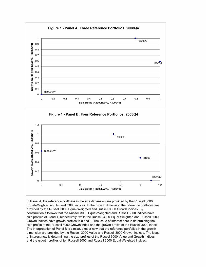
for 2008Q4 of the locations of the mcw =Russell 3000, ew =Russell 3000 Equal-Weighted,
and gw =Russell 3000 Growth portfolios in S-G space over the Russell 3000 stock universe
is provided in Figure 1(a).
Insert Figure 1 Here
To determine the proportions in which our three reference portfolios must be combined
to generate a portfolio with the same S and G profiles as w, it is necessary to solve the
following system of two simultaneous equations:
⎛⎜⎝ S(ew)
G(ew)
⎞⎟⎠+ μ1
⎛⎜⎝ S(mcw)− S(ew)
G(mcw)− G(ew)
⎞⎟⎠+ μ2
⎛⎜⎝ S(gw)− S(ew)
G(gw)− G(ew)
⎞⎟⎠ =
⎛⎜⎝ S(w)
G(w)
⎞⎟⎠ .
(12)
The only unknowns in (12) are μ1 and μ2. The terms S(w) and G(w) on the righthand side
of (12) denote the S and G profiles of the portfolio w calculated from (1).
Making the substitutions S(mcw) = G(gw) = 1 and S(ew) = G(ew) = 0, (12) simpli-
fies to the following:
μ1 + μ2S(gw) = S(w), (13)
μ1G(mcw) + μ2 = G(w). (14)
These equations yield the following solutions for μ1 and μ2:
μ1 =S(w)− S(gw)G(w)
1− S(gw)G(mcw), (15)
μ2 =G(w)− G(mcw)S(w)
1− S(gw)G(mcw). (16)
12

A tailored benchmark portfolio w that has the same S and G profile as the portfolio w
can now be derived as follows:
wn = μ1mcwn + μ2gwn + (1− μ1 − μ2)ewn, for n = 1, . . . , N, (17)
with μ1 and μ2 derived from (15) and (16). That S(w) = S(w) can be verified as follows:
S(w) = μ1S(mcw) + μ2S(gw) + (1− μ1 − μ2)S(ew) = μ1 + μ2S(gw),
since S(mcw) = 1 and S(ew) = 0. Now substituting for μ1 and μ2 from (15) and (16), we
obtain that:
S(w) =
[S(w)− S(gw)G(w)
1− S(gw)G(mcw)
]+
[G(w)− G(mcw)S(w)
1− S(gw)G(mcw)
]S(gw) = S(w).
In the same way it can be shown that G(w) = G(w).8
The one-dimensional least-squares optimization result for w generalizes to higher di-
mensions. In two dimensions, we define the distance D between the portfolio w and a
portfolio w formed by taking linear combinations of the three reference portfolios as fol-
lows:
D =
√√√√ N∑n=1
(wn − wn)2,
where now
wn = μ1 mcwn +μ2 gwn + (1−μ1 −μ2)ewn. (18)
8Although we do not do it here, this approach could also be used to construct a growth style benchmarkthat is matched to multiple dimensions of a portfolio’s value-growth characteristics, such as book value,earnings, dividends, sales, etc as recommended by CDL.
13

Hence we can rewrite D as follows:
D =
√√√√ N∑n=1
[wn −μ1 mcwn −μ2 gwn − (1−μ1 −μ2)ewn]2. (19)
Differentiating with respect to μ1 and μ2, we obtain first order conditions which on re-
arrangement are identical to (13) and (14) (see Appendix B). Hence the solutions for μ1
and μ2 in this least-squares minimization problem are the same as those given in (15) and
(16) above. It follows that w = w, and hence that w is the linear combination of the three
reference portfolios that in a least-squares sense most closely approximates the portfolio
w, as well as having the same S and G profile as w.
3.2. Using four reference portfolios
Suppose now we have four reference portfolios. The first issue is to ensure that these ref-
erence portfolios are mutually compatible. A good example of incompatible portfolios is
provided by the Russell 3000, Russell 3000 Value and Russell 300 Growth portfolios. Since
these portfolios are not linearly independent (the Russell 3000 portfolio equals the sum
of the Russell 3000 Growth and Russell 3000 Value portfolios), this combination of refer-
ence portfolios will generate a singular matrix in the system of simultaneous equations
below. In the empirical comparisons in the next section, therefore, we use mcw =Russell
1000, ew =Russell 3000 Equal-Weighted, vw =Russell 3000 Value and gw =Russell 3000
Growth as our reference portfolios, where our S profiles are obtained by setting mcw = lg
and ew = sm in (1) and our G profiles by setting gw = lg and vw = sm in (1). An em-
pirical example of the locations of mcw =Russell 1000, ew =Russell 3000 Equal-Weighted,
vw =Russell 3000 Value and gw =Russell 3000 Growth portfolios in S-G space is provided
in Figure 1(b).
As it stands, the system for constructing tailored benchmark portfolios is overdeter-
14

mined when there are four reference portfolios. This means that we can generate an
infinite number of benchmark portfolios that will be tailored to have the same S and G
profiles as a portfolio w.
To choose between them, we can again use least squares optimization. A linear combi-
nation of the four reference portfolios takes the following form:
wn = μ1mcwn +μ2gwn +μ3vwn + (1−μ1 −μ2 −μ3)ewn, for n = 1, . . . , N (20)
We now define the distance D between the portfolio w and w as follows:
D =
√√√√ N∑n=1
[wn −μ1 mcwn −μ2 gwn −μ3 vw− (1−μ1 −μ2 −μ3)ewn]2. (21)
Differentiating with respect to μ1, μ2 and μ3, the first-order conditions yield a system of
three simultaneous equations in three unknowns (see Appendix C). The solutions for μ1,
μ2 and μ3 are obtained as follows:9
⎛⎜⎜⎜⎜⎝
μ1
μ2
μ3
⎞⎟⎟⎟⎟⎠ =
⎛⎜⎜⎜⎜⎝
1 S(gw) S(vw)
SG(mcw) 1 SG(vw)
SV(mcw) SV(gw) 1
⎞⎟⎟⎟⎟⎠
−1 ⎛⎜⎜⎜⎜⎝
S(w)
SG(w)
SV(w)
⎞⎟⎟⎟⎟⎠ . (22)
Substituting the solutions for μ1, μ2 and μ3 obtained from (22) into (20), we obtain the
portfolio w formed from linear combinations of the four reference portfolios mcw, ew, gw
and vw that most closely approximates in a least-squares sense the portfolio w.
It is shown in Appendix D that the size and growth profiles of w are the same as those
of w (i.e., that S(w) = S(w) and G(w) = G(w)).
9The terms SG(mcw), SG(vw), SV(mcw) and SV(gw) in (22) are defined in Appendix C.
15

4. Disentangling Size and Growth Effects
Changing the parameter λ in (6) may change the style profile in other dimensions as well
as the one on we are focusing. For example, the Russell 3000 and Russell 3000 Equal-
Weighted portfolios differ in both their S and G profiles in Figure 1(a). To obtain a pure
measure of the impact of changes in S on performance holding G fixed, we need to take
linear combinations of two reference portfolios with the same G profile. Such reference
portfolios can easily be constructed using a variant on our basic method.
Returning to the three reference-portfolio setting, we seek two portfolios w0 and w1
that are linear combinations of our three reference portfolios and have the following prop-
erties:
S(w0) = 0, G(w0) = G, S(w1) = 1, G(w1) = G.
The coordinates of w0 and w1 in size-growth space are illustrated in Figure 2.
Insert Figure 2 Here
Setting S(w0) = 0 and G(w0) = G in (15) and (16), the portfolio w0 can be calculated
as follows:
μ01 =
−S(gw)G1− S(gw)G(mcw)
,
μ02 =
G1− S(gw)G(mcw)
.
Using these weights, we obtain that
w0n = ewn +μ0
1(mcwn − ewn) +μ02(gwn − ewn), for n = 1, . . . , N.
16

Similarly, setting S(w1) = 1 and G(w1) = G in (15) and (16), it follows that
μ11 =
1− S(gw)G1− S(gw)G(mcw)
,
μ12 =
G− G(mcw)
1− S(gw)G(mcw),
and hence
w1n = ewn +μ1
1(mcwn − ewn) +μ12(gwn − ewn), for n = 1, . . . , N.
Having constructed these two portfolios w0 and w1 that have the same G profiles, if
we now take linear combinations of w0 and w1, we can vary the S profile while holding
the G profile fixed at G, and hence observe the pure effect of size on our performance
benchmarks. This is achieved by varying the parameter θ in the expression below:
wn = θw0n + (1−θ)w1
n, for n = 1, . . . , N.
When θ = 1 we are at the coordinates (0, G) in Figure 2. As θ falls, we move along the
horizontal line connecting w0 and w1, until at θ = 0 we arrive at (1, G).
In an analogous manner we can likewise construct portfolios that allow us to vary the
G profile while holding the S profile fixed. This methodology again generalizes to higher
dimensions.
5. Conditional Version of Our Methods
CDL demonstrate how characteristic-matched benchmarks constructed by sorting stocks
by growth conditional on size tend to generate lower tracking error volatilities than in-
dependent sorts on size and growth. Our methods thus far described treat each style
17

dimension independently. Conditional variants, however, could be constructed by elimi-
nating from the reference portfolios in the value-growth dimension (e.g., the Russell 3000
Value and Growth portfolios) all stocks not held in the portfolio w. The remaining stocks
in the reference portfolios would then be rescaled so that their shares sum to 1. For exam-
ple, the growth profile of a small-cap manager would then be calculated from reference
portfolios in the value-growth dimension that are themselves by construction also small
cap. The reference portfolios in the value-growth dimension therefore would themselves
be tailored to each particular portfolio w. This conditional approach should tend to reduce
the tracking error volatilities of our methods.
Brands, Brown and Gallagher (2005) (BBG) draw a distinction between two aspects of
active management. A manager must first decide which stocks to include in a portfolio,
and, second, in what proportions to hold these stocks. BBG refer to these activities as
‘stock picking’ and ‘portfolio construction’. One feature of the conditional version of our
method is that it constructs benchmarks that focus exclusively on the latter activity (i.e.,
portfolio construction). In this sense, our conditional method could provide a useful com-
plement to our unconditional method and existing methods for benchmark construction.
6. An Application to Fund Managers and Indices
6.1. The data set
Our data set consists of a sample of 1183 US institutional fund manager from the Russell
database covering the period 2002Q2 to 2009Q3. We select funds for which at least 80
percent of the provided security IDs were matched to the Russell 3000 universe of stocks.
Some of the unmatched security IDs contain cash or bond holdings and others are not
included in the Russell 3000 listing of stocks. When calculating tracking error volatilities,
we only consider managers for which we have at least 12 consecutive quarters of data.
18

This reduces our sample of managers to 275.10
6.2. The cross-section of index and fund style
A scatter plot of fund manager size and growth style profiles provides a useful indication
of the range and variability of fund manager behavior. One such example is provided in
Figure 3 for the 464 fund managers present in our data set in 2008Q4 (this was the quarter
with the most fund managers). The reference portfolios in Figure 3 are sm=Russell 3000
Equal-Weighted and lg=Russell 1000 in the size dimension, while sm=Russell 3000 Value
and lg=Russell 3000 Growth in the value-growth dimension.
Insert Figure 3 Here
From Figure 3 we can see that not a single fund manager holds a portfolio with a size
profile smaller than the Russell 3000 Equal-Weighted index, 40 out of 464 portfolios have
larger size profiles than the Russell 1000 index, 2 have smaller growth profiles than the
Russell 3000 Value index and 13 have larger growth profiles than the Russell 3000 Growth
index. It is also striking how the range of growth profiles fans out as the size profile rises
from 0 to 0.8, after which the growth profile range starts to fall again. The variation of
growth styles across funds therefore reaches a maximum when the size profile is about
0.8.
Figure 4 provides an equivalent scatter plot for some of the main Russell indices. The
reference portfolios in Figure 4 are the same as in Figure 3. Hence by construction, the
Russell 3000 Value and Growth indices have growth profile of 0 and 1 respectively, while
the Russell 3000 Equal-Weighted and Russell 1000 indices have size profiles of 0 and 1.
10The choice of the number of consecutive quarters required for inclusion is somewhat subjective. CDLfor example require 16 consecutive quarters. We prefer 12 since the gains in sample size (275 instead of 164funds) in our opinion outweighs the disadvantages of having a shorter time horizon for some managers. Asa robustness check we also calculate results based on the requirement of 16, 20 and 24 consecutive quartersrespectively. We find that the results for these alternatives differ only marginally from those obtained for 12consecutive quarters.
19
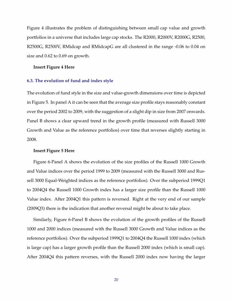
Figure 4 illustrates the problem of distinguishing between small cap value and growth
portfolios in a universe that includes large cap stocks. The R2000, R2000V, R2000G, R2500,
R2500G, R2500V, RMidcap and RMidcapG are all clustered in the range -0.06 to 0.04 on
size and 0.62 to 0.69 on growth.
Insert Figure 4 Here
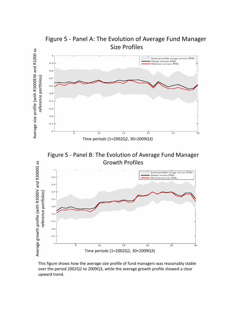
6.3. The evolution of fund and index style
The evolution of fund style in the size and value-growth dimensions over time is depicted
in Figure 5. In panel A it can be seen that the average size profile stays reasonably constant
over the period 2002 to 2009, with the suggestion of a slight dip in size from 2007 onwards.
Panel B shows a clear upward trend in the growth profile (measured with Russell 3000
Growth and Value as the reference portfolios) over time that reverses slightly starting in
2008.
Insert Figure 5 Here
Figure 6-Panel A shows the evolution of the size profiles of the Russell 1000 Growth
and Value indices over the period 1999 to 2009 (measured with the Russell 3000 and Rus-
sell 3000 Equal-Weighted indices as the reference portfolios). Over the subperiod 1999Q1
to 2004Q4 the Russell 1000 Growth index has a larger size profile than the Russell 1000
Value index. After 2004Q1 this pattern is reversed. Right at the very end of our sample
(2009Q3) there is the indication that another reversal might be about to take place.
Similarly, Figure 6-Panel B shows the evolution of the growth profiles of the Russell
1000 and 2000 indices (measured with the Russell 3000 Growth and Value indices as the
reference portfolios). Over the subperiod 1999Q1 to 2004Q4 the Russell 1000 index (which
is large cap) has a larger growth profile than the Russell 2000 index (which is small cap).
After 2004Q4 this pattern reverses, with the Russell 2000 index now having the larger
20

growth profile. The gap again narrows at the end of the sample.
These findings qualify a standard perception in the literature that large cap stocks tend
to have a growth tilt (see for example CDL who discuss this point in the process of ex-
plaining why conditional sorts on size should be preferred to independent sorts). While
this is true for the first half of our sample, this pattern reverses after 2004.
Insert Figure 6 Here
6.4. Tracking error volatilities of tailored performance benchmarks and excess returns
of funds
The tracking error of a benchmark is calculated as the difference between the performance
of the portfolio and the performance of its benchmark. Tracking error volatility measured
by the annualized standard deviation of tracking error over a sample of quarters is often
used in the literature to judge the appropriateness of benchmarks (see for example CDL
and CP). A lower tracking error volatility implies that the performance differential be-
tween a portfolio and its benchmark has a larger systematic component, thus increasing
the usefulness of the benchmark.
Average tracking error volatilities of our tailored performance benchmarks and ex-
cess returns of funds are provided in Table 1. In the first column of Table 1 we replicate
the value-weight conditional sort (i.e., quarterly size, within-size, BM) method used by
CDL. This is their preferred method since it outperforms benchmarks constructed from
attribute-matched independent sorts of portfolios, the three-factor time-series model and
cross-sectional regressions of returns on stock characteristics.11 Hence we use the CDL
value-weight conditional sort method as a point of reference with which to assess the
performance of our tailored benchmarks.
11CDL argue also for the use of composite value-growth measures. Our method can be easily extendedin this direction by defining more than one dimension in the value-growth domain, and then matchingportfolios and benchmarks by style in each dimension. We do not pursue this idea here, however, andhence to improve comparability likewise do not consider CDL’s composite value-growth measures either.
21

Insert Table 1 Here
Seven of our tailored benchmarks are compared with the CDL tailored benchmark and
a Russell 3000 benchmark in Table 1. Our seven benchmarks are described below. The first
three are absolute benchmarks in the sense that their underlying size and growth profiles
are monotonic functions of absolute measures of size (Sast) and growth (Gast) (see section
2.1 and Appendix A). The remaining four benchmarks are relative in the sense that their
underlying size and growth profiles are defined relative to two reference portfolios in each
style dimension.
1. Abs S: one-dimensional size benchmark: lg=Russell 3000, sm=Russell 3000 Equal-
Weighted
2. Abs G: one-dimensional growth benchmark: lg = gw (where gw is defined in (4)),
sm=Russell 3000 Equal-Weighted
3. Abs SG: two-dimensional size-growth benchmark: lgS=Russell 3000, smS=Russell 3000
Equal-Weighted, lgG = gw, smG=Russell 3000 Equal-Weighted
4. Rel S: one-dimensional size benchmark: lg=Russell 1000, sm=Russell 3000 Equal-
Weighted
5. Rel G: one-dimensional growth benchmark lg=Russell 3000 Growth, sm=Russell 3000
Value
6. Rel SG(3): two-dimensional size-growth benchmark: lgS=Russell 1000, smS=Russell
3000 Equal-Weighted, lgG=Russell 3000 Growth, smG=Russell 3000 Equal-Weighted
7. Rel SG(4): two-dimensional size-growth benchmark: lgS=Russell 1000, smS=Russell
3000 Equal-Weighted, lgG=Russell 3000 Growth, smG=Russell 3000 Value.
Based on median tracking error volatility, the best performer is Rel G, followed in or-
22

der by CDL, Abs SG, Rel SG(3), Russell 3000, Rel SG(4), Abs S, Rel S and lastly Abs G.
The mean tracking error volatility ranking differs only in that the order of Rel G and
CDL is reversed.12 We have a number of observations on the results presented in Table 1.
First, it is perhaps surprising that Rel G has a lower tracking error volatility than both
Rel SG(3) and Rel SG(4) given that the Rel SG(3) and Rel SG(4) benchmarks are more
closely tailored to the individual funds. The lower tracking error volatility of Rel G sug-
gests that its tailored benchmarks adjust over time in a way that matches more closely
shifts in portfolio holdings, and hence that value/growth orientation is a major driver of
shifts in funds’ approaches to stock picking. Second, the fact that Rel SG(3) has a lower
tracking error volatility than Rel SG(4) is also interesting given that by construction the
Rel SG(4) benchmark portfolio must be closer to the underlying portfolio (i.e., it must
have a lower distance measure as defined in (10)) than the Rel SG(3) benchmark portfo-
lio. Again the explanation is probably that the optimization method used by Rel SG(4)
causes the benchmark portfolio to adjust more over time than the portfolio itself. Hence a
better fit in each specific period may act to increase tracking error volatility. Third, while
Rel G significantly outperforms Abs G, we find that Abs SG has a lower tracking error
volatility than either Rel SG(3) or Rel SG(4). It is therefore not clear which out of relative
and absolute versions of our method should be preferred. Finally, the results in Table 1
demonstrate that at least some of our methods are competitive in terms of tracking error
volatility with the best of the methods considered by CDL, while at the same time being
conceptually simpler and easier to compute. Furthermore, the fact that the CDL method
uses conditional sorts on size in the value-growth dimension while our methods do not,
in some sense biases the comparison against our methods. Conditional versions of our
methods, constructed in the manner outlined above, may perform even better.
12Exactly the same median and mean rankings of methods are obtained when the comparison is restrictedto funds present for at least 16 consecutive quarters.
23

6.5. Activity and performance
A large literature exists on the topic of whether active fund managers on average outper-
form passive managers (see for example (see for example Wermers, 2000). Cremers and
Petajisto (2009), again henceforth CP, go further and consider whether more active man-
agers outperform less active managers. CP distinguish between two notions of activity,
which they refer to as stock selection and factor timing. Stock selection is a cross-section
concept, which measures the deviation of a portfolio from its benchmark in a particular
period. Factor timing can be measured by the tracking error volatility of managers rel-
ative to their benchmarks. CP find a positive relationship between stock selection and
performance but no clear relationship between factor timing activity and performance.
Here we revisit this issue in a cross-section context using our measure of activity as
defined in (10).13 Activity quintiles and their corresponding average excess returns cal-
culated using three of our tailored benchmarks – Rel S, Rel G and Rel SG(4) – and the
Russell 3000 as benchmark are shown in Table 2.
Insert Table 2 Here
The results in Table 2 are striking in that we observe the opposite result to that obtained
by CP. That is, we find that more active funds perform worse than less active funds.
There are a number of differences between our study and that of CP that may explain
our finding. First, there is very little overlap in our time horizons. Our data set covers the
period 2002Q2 to 2009Q3, while the CP’s covers the period 1990 to 2003. Second, our time
horizon is shorter and includes the financial crisis that started in 2007. Third, our data
set consists of institutional fund managers as opposed to mutual fund managers. Hence
the lack of overlap in our samples applies to fund managers as well as the time horizon.
13We could in principle also use our approach to investigate the link between tracking error volatility andperformance.
24

Fourth, our performance benchmarks are matched in terms of style to each fund manager,
while CP only achieve an approximate match by searching over 19 well-known indices
to find the one that minimizes their measure of activity and assigning this as the bench-
mark for that particular manager in that particular period. Finally, our activity measure is
least squares based while CP’s minimizes the absolute deviation between portfolios and
benchmarks.
To determine whether the financial crisis is influencing our results, we try restricting
the time span of our data set to 2002Q2-2007Q1. As shown in Table 2, excluding the fi-
nancial crisis makes the inverse relationship between performance and activity if anything
even stronger than before. To assess the impact of better matching of managers and perfor-
mance benchmarks on the observed link between activity and performance we recalculate
activity and excess return for each manager using the Russell 3000 as the benchmark. The
use of a common benchmark likewise acts to further accentuate the inverse relationship
between activity and performance observed in Table 2. Put another way, the failure to
use tailored benchmarks seems to cause the link between activity and performance to be
overstated.
Our finding therefore suggests that the relationship between activity and performance
may be dependent on the time horizon or sample of fund managers and hence perhaps
more complex than previously thought.
6.6. Disentangled Size and Growth Effects
We illustrate the impact on performance of changes in size holding the growth profile
fixed in a three-reference-portfolio context. The Russell 3000 Equal-Weighted, Russell 3000
and Russell 3000 Growth indices are used as the reference portfolios. Figure 7 contrasts
the impact of varying size by taking linear combinations of our three reference portfo-
lios on total return for each of the four quarters in 2008. The dashed line in each case is
25

obtained by taking linear combinations of the Russell 3000 Equal-Weighted and Russell
3000 reference portfolios. As one moves along this dashed line, both the growth and size
profiles change. These effects are disentangled by the three parallel lines in each caption
of Figure 7. Each of these lines fixes the growth profile G at a particular value (0, 0.5 or
1), and then allows size to vary. By construction, the slope of these lines is independent of
the value of G.
Insert Figure 7 Here
The most striking feature of Figure 7 is how holding growth fixed can reverse the sign
of the slope of the total return line. Over our whole data set of 44 quarters covering the
period 1999Q1 to 2009Q4 (our time horizon for the indices is larger than for the fund
manager data set) we find that holding growth fixed acts to change the sign of the slope
of the total return line for 29 of 44 quarters. By implication, when determining the impact
of changes in size on performance it is important to control for changes in style in other
dimensions.
A second feature of Figure 7 worth noting is the sensitivity of total return for any given
size profile to the reference growth profile. In 2008Q3, total return for any given size pro-
file varies by more than 9 percentage points as the reference growth profile varies between
0 and 1. By contrast, in 2008Q1 and 2008Q4 this difference is less than 2 percentage points,
which while much smaller is still not trivial.
7. Conclusion
Characteristic-matched performance benchmarks obtained from portfolio holdings data
are typically constructed using a bottom-up approach which first matches individual
stocks to one of a number of discrete portfolios with similar style characteristics. The
overall benchmark is then calculated by taking a weighted average of the excess returns
26

on each of the individual stocks. We have proposed here an alternative methodology
that avoids this bottom-up approach and generates direct matches between portfolios and
benchmarks.
Our method also has the advantage of conceptual and computational simplicity. Our
tailored performance benchmarks can be easily calculated by taking linear combinations
of off-the-shelf indices such as the Russell 3000, Russell 3000 Growth and Russell 3000
Value. It can be applied in multiple style dimensions, and generates tracking error volatil-
ities that are comparable with the best existing methods. In addition, our method provides
new measures of style that are of interest in their own right and which shed new light on
both the cross-section of index and fund manager style, and the evolution over time of
index and fund manager style. It also leads naturally to new measures of activity that
focus on deviations of a portfolio’s holdings from those of its matched style benchmark,
and perhaps a new perspective on the link between performance and activity.
Our new approach to constructing characteristic-matched performance benchmarks
provides market participants with a new set of tools for evaluating fund style and perfor-
mance, and opens up a new direction for research on the construction of characteristic-
matched performance benchmarks distinct from the bottom-up approach that has domi-
nated the literature in recent years.
27

References
Brands, Simone, Stephen J. Brown and David R. Gallagher (2005): “Portfolio Concentration andInvestment Manager Performance”, International Review of Finance, 5 (3-4), 149–174.
Brown, Stephen J. and William N. Goetzmann (1997): “Mutual fund styles”, Journal of FinancialEconomics, 43 (3), 373–399.
Carhart, Mark M. (1997): “On Persistence in Mutual Fund Performance”, Journal of Finance, 52 (1),57–82.
Chan, Louis K. C., Hsiu-Lang Chen and Josef Lakonishok (2002): “On Mutual Fund InvestmentStyles”, Review of Financial Studies, 15 (5), 1407–1437.
Chan, Louis K. C., Stephen G. Dimmock and Josef Lakonishok (2009): “Benchmarking MoneyManager Performance: Issues and Evidence”, Review of Financial Studies, 22 (11), 4553–4599.
Cremers, Martijn and Antti Petajisto (2009): “How Active is Your Fund Manager? A New MeasureThat Predicts Performance”, Review of Financial Studies, 22 (9), 3329–3365.
Daniel, Kent, Mark Grinblatt, Sheridan Titman and Russ Wermers (1997): “Measuring MutualFund Performance with Characteristic-Based Benchmarks”, Journal of Finance, 52 (3), 1035–58.
diBartolomeo, Dan and Erik Witkowski (1997): “Mutual Fund Misclassification: Evidence Basedon Style Analysis”, Financial Analysts Journal, 53 (5), 32–43.
Fama, Eugene F and Kenneth R French (1992): “The Cross-Section of Expected Stock Returns”,Journal of Finance, 47 (2), 427–65.
–———— (1996): “Multifactor Explanations of Asset Pricing Anomalies”, Journal of Finance, 51 (1),55–84.
Jensen, Michael C. (1967): “The Performance Of Mutual Funds In The Period 1945-1964”, Journalof Finance, 23 (2), 389–416.
–———— (1969): “Risk, The Pricing of Capital Assets, and the Evaluation of Investment Portfo-lios”, Journal of Business, 42 (2), 167–247.
Kacperczyk, Marcin, Clemens Sialm and Lu Zheng (2005): “On the Industry Concentration of Ac-tively Managed Equity Mutual Funds”, Journal of Finance, 60 (4), 1983–2011.
Kothari, S.P. and Jerold B. Warner (2001): “Evaluating Mutual Fund Performance”, Journal of Fi-nance, 56 (5), 1985–2010.
Russell Investments (2008): “US Equity Indexes: Institutional Benchmark Survey”,www.russell.com/indexes/documents/Benchmark Usage.pdf.
Sharpe, William F . (1988): “Determining a Fund’s Effective Asset Mix”, Investment ManagementReview, 2 (6), 59–69.
28

–———— (1992): “Asset allocation Management style and performance measurement”, The Jour-nal of Portfolio Management, 18 (2), 7–19.
Wermers, Russ (2000): “Mutual Fund Performance: An Empirical Decomposition into Stock-Picking Talent, Style, Transactions Costs, and Expenses”, Journal of Finance, 55 (4), 1655–1695.
Appendix
A. Constructing Size/Growth Profiles that are Monotonic Functions of Absolute Mea-
sures of Size/Growth
Let mcw and ew denote respectively a market-cap-weighted and equal-weighted portfolio.
Setting lg = mcw and sm = ew in (1), we obtain that
P(w) =
∑Nn=1[(mcwn − ewn)(wn − ewn)]∑N
n=1(mcwn − ewn)2, (A.1)
where
mcwn =pnqn∑N
m=1 pmqm, ewn =
1N
, for n = 1, . . . , N. (A.2)
By construction,∑N
n=1 mcwn =∑N
n=1 ewn = 1. In what follows it is assumed that there
exist at least two stocks for which ewn �= mcwn. Otherwise the style profile P(w) below is
not defined.
In this case P(w) is a monotonic (linear) function of the absolute size measure S∗(w) as
defined in (2). This can be demonstrated as follows:
P(w) =
∑Nn=1[(mcwn − ewn)(wn − ewn)]∑N
n=1(mcwn − ewn)2=
∑Nn=1(wnmcwn)− 1/N∑N
n=1(mcw2n)− 1/N
= αS +βSS∗(w),
(A.3)
where
αS = − 1/N∑Nn=1(mcw2
n)− 1/N, βS =
1
(∑N
n=1 pnqn)(∑N
n=1(mcw2n)− 1/N)
.
29
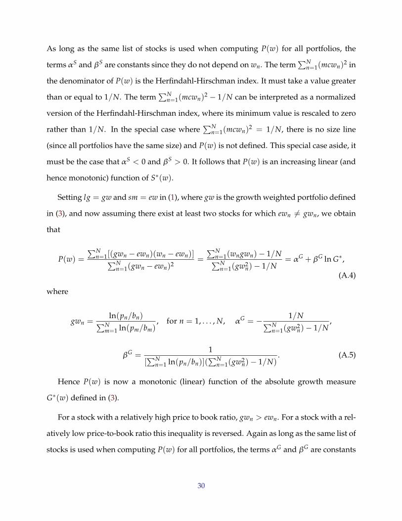
As long as the same list of stocks is used when computing P(w) for all portfolios, the
termsαS and βS are constants since they do not depend on wn. The term∑N
n=1(mcwn)2 in
the denominator of P(w) is the Herfindahl-Hirschman index. It must take a value greater
than or equal to 1/N. The term∑N
n=1(mcwn)2 − 1/N can be interpreted as a normalized
version of the Herfindahl-Hirschman index, where its minimum value is rescaled to zero
rather than 1/N. In the special case where∑N
n=1(mcwn)2 = 1/N, there is no size line
(since all portfolios have the same size) and P(w) is not defined. This special case aside, it
must be the case that αS < 0 and βS > 0. It follows that P(w) is an increasing linear (and
hence monotonic) function of S∗(w).
Setting lg = gw and sm = ew in (1), where gw is the growth weighted portfolio defined
in (3), and now assuming there exist at least two stocks for which ewn �= gwn, we obtain
that
P(w) =
∑Nn=1[(gwn − ewn)(wn − ewn)]∑N
n=1(gwn − ewn)2=
∑Nn=1(wngwn)− 1/N∑N
n=1(gw2n)− 1/N
= αG +βG ln G∗,
(A.4)
where
gwn =ln(pn/bn)∑N
m=1 ln(pm/bm), for n = 1, . . . , N, αG = − 1/N∑N
n=1(gw2n)− 1/N
,
βG =1
[∑N
n=1 ln(pn/bn)](∑N
n=1(gw2n)− 1/N)
. (A.5)
Hence P(w) is now a monotonic (linear) function of the absolute growth measure
G∗(w) defined in (3).
For a stock with a relatively high price to book ratio, gwn > ewn. For a stock with a rel-
atively low price-to-book ratio this inequality is reversed. Again as long as the same list of
stocks is used when computing P(w) for all portfolios, the termsαG and βG are constants
30

(i.e., they do not depend on wn). The growth variant of the Herfindahl-Hirschman index∑N
n=1(gwn)2 must be greater than 1/N, except in the special case where all stocks have
the same price-to-book ratio. In this case, all portfolios have the same growth profile and
hence there is no growth line. Also, the growth weights gwn will be negative for stocks
with a price-to-book value of less than one. The presence of negative weights, however,
does not create any problems here. The only complication it creates is that it is hence the-
oretically possible that βG may be negative. When this happens, P(w) is a monotonically
decreasing rather than increasing function of G∗.
B. Demonstration that w is the Linear Combination of Three Reference Portfolios in
Two Style Dimensions that in a Least-Squares Sense Most Closely Approximates
the Portfolio w.
Differentiating (19) with respect to μ1 and μ2 generates the following first order condi-
tions:
∂D∂μ1
=
∑Nn=1(ewn −mcwn)[wn − (1−μ1 −μ2)ewn −μ1mcwn −μ2gwn]∑N
n=1[wn −μ1 mcwn −μ2 gwn − (1−μ1 −μ2)ewn]2= 0,
∂D∂μ2
=
∑Nn=1(ewn − gwn)[wn − (1−μ1 −μ2)ewn −μ1mcwn −μ2gwn]∑N
n=1[wn −μ1 mcwn −μ2 gwn − (1−μ1 −μ2)ewn]2= 0.
These first order conditions can be rearranged as follows:
N∑n=1
(ewn −mcwn)(wn − ewn) +μ1
N∑n=1
(ewn −mcwn)(ewn −mcwn)
+μ2
N∑n=1
(ewn −mcwn)(ewn − gwn) = 0,
N∑n=1
(ewn − gwn)(wn − ewn) +μ1
N∑n=1
(ewn −mcwn)(ewn −mcwn)
31

+μ2
N∑n=1
(ewn −mcwn)(ewn − gwn) = 0.
Dividing through the first equation by∑N
n=1(mcwn − ewn)2 and the second equation by∑N
n=1(gwn − ewn)2 we obtain that
S(w)−μ1 −μ2
∑Nn=1(mcwn − ewn)(gwn − ewn)∑N
n=1(gwn − ewn)2= 0,
G(w)−μ1
∑Nn=1(mcwn − ewn)(gwn − ewn)∑N
n=1(gwn − ewn)2−μ2 = 0.
Noticing now that∑N
n=1(mcwn − ewn)(gwn − ewn)/∑N
n=1(gwn − ewn)2 = S(gw) and∑N
n=1(mcwn − ewn)(gwn − ewn)/∑N
n=1(gwn − ewn)2 = G(mcw), the first order condi-
tions reduce to the following:
S(w)−μ1 −μ2S(gw) = 0, (B.1)
G(w)−μ1G(mcw)−μ2 = 0. (B.2)
On closer inspection (B.1) is identical to (13) while (B.2) is identical to (14). Hence the
solutions for μ1 and μ2 in this least-squares minimization problem are the same as those
given in (15) and (16) above. It follows that D is minimized when w equals w.14 Hence
w is the linear combination of the three reference portfolios that in a least-squares sense
most closely approximates the portfolio w, as well as having the same S and G profile as
w.
14D is defined in (7), w in (18) and w in (17).
32

C. Derivation of the 4-reference portfolio simultaneous equation system
Differentiating (D.3) with respect to μ1, μ2 and μ3, after rearrangement we obtain the
following first order conditions:
∑Nn=1(mcwn − ewn)(wn − ewn)∑N
n=1(mcwn − ewn)2−μ1 −μ2
∑Nn=1(mcwn − ewn)(gwn − ewn)∑N
n=1(mcwn − ewn)2
−μ3
∑Nn=1(mcwn − ewn)(vwn − ewn)∑N
n=1(mcwn − ewn)2= 0, (C.1)
∑Nn=1(gwn − ewn)(wn − ewn)∑N
n=1(gwn − ewn)2−μ1
∑Nn=1(gwn − ewn)(mcwn − ewn)∑N
n=1(gwn − ewn)2−μ2
−μ3
∑Nn=1(gwn − ewn)(vwn − ewn)∑N
n=1(gwn − ewn)2= 0, (C.2)
∑Nn=1(vwn − ewn)(wn − ewn)∑N
n=1(vwn − ewn)2−μ1
∑Nn=1(vwn − ewn)(mcwn − ewn)∑N
n=1(vwn − ewn)2
−μ2
∑Nn=1(vwn − ewn)(gwn − ewn)∑N
n=1(vwn − ewn)2−μ3 = 0. (C.3)
These equations can in turn be rewritten as follows:
S(w)−μ1 −μ2S(gw)−μ3S(vw) = 0, (C.4)
S(w)−μ1SG(mcw)−μ2 −μ3SG(vw) = 0, (C.5)
SV(w)−μ1SV(mcw)−μ2SV(gw)−μ3 = 0, (C.6)
33

where
SG(w) =
∑Nn=1(gwn − ewn)(wn − ewn)∑N
n=1(gwn − ewn)2,
SG(mcw) =
∑Nn=1(gwn − ewn)(mcwn − ewn)∑N
n=1(gwn − ewn)2,
SG(vw) =
∑Nn=1(gwn − ewn)(vwn − ewn)∑N
n=1(gwn − ewn)2,
SV(w) =
∑Nn=1(vwn − ewn)(wn − ewn)∑N
n=1(vwn − ewn)2,
SV(mcw) =
∑Nn=1(vwn − ewn)(mcwn − ewn)∑N
n=1(vwn − ewn)2,
SV(gw) =
∑Nn=1(vwn − ewn)(gwn − ewn)∑N
n=1(vwn − ewn)2.
The terms SG(w), SG(mcw), SG(vw), SV(w), SV(mcw) and SV(gw) in (C.5) and (C.6)
require some explanation. SG(w) measures the location of the portfolio w in the one
dimensional space with the ew portfolio located at zero and the gw portfolio located at 1.
At first glance this seems to be simply the growth profile of w. However, this is not correct
since in this relative context the points of reference in growth space are now the gw and
vw portfolios rather than the gw and ew portfolios. SV(w) similarly measures the location
of the portfolio w in the one dimensional space with the ew portfolio located at zero and
the vw portfolio located at 1. SG(mcw) measures the location of the mcw portfolio in the
one dimensional space with the ew portfolio located at zero and the gw portfolio located
at 1. The other terms can be explained in analogous ways.
The equations (C.4), (C.5) and (C.6) can now be written in matrix notation as stated in
(22).
34

D. Derivation of the Size and Growth Profiles of w
To verify that S(w) = S(w), starting from (20) and using the fact that S(mcw) = 1 and
S(ew) = 0, we obtain that
S(w) = μ1 +μ2S(gw) +μ3S(vw). (D.1)
The result now follows directly from a comparison of (C.4) and (D.1).
The fact that G(w) = G(w) is less obvious. This requirement is subsumed in (C.5) and
(C.6). The easiest way to see that this must be true is to reparameterize the w portfolio as
follows:
wn = μ1gwn +μ2mcwn +μ3ewn + (1−μ1 −μ2 −μ3)vwn, for n = 1, . . . , N, (D.2)
which in turn implies that the distance between w and w is also reparameterized:
D =
√√√√ N∑n=1
[wn −μ1 gwn −μ2 mcwn −μ3 ew− (1−μ1 −μ2 −μ3)vwn]2. (D.3)
Given this reparameterization, one of the first order conditions now reduces to
G(w)−μ1 −μ2S(mcw)−μ3S(ew) = 0. (D.4)
Now starting from (D.2), and using the fact that G(gw) = 1 and G(vw) = 0, we obtain
that
G(w) = μ1 +μ2S(mcw) +μ3S(ew). (D.5)
The result now follows directly from a comparison of (D.4) and (D.5).
35

Table 1: Benchmark Tracking Error Volatilities, Excess Returns and Activity for Funds (2002Q2-2009Q3)
TE Volatility CDL Abs_S Abs_G Abs_SG Rel_S Rel_G Rel_SG(3) Rel_SG(4) R3000Mean 4.8588 5.7604 7.7792 5.0986 5.7921 4.9016 5.2546 5.5443 5.2965Median 4.4690 5.5101 7.5945 4.8505 5.5578 4.4663 4.8972 5.1926 4.9538Stdev. 1.7807 2.1238 1.5361 1.7152 2.1464 1.9764 1.8477 1.9899 2.0942Min 1.2717 2.1075 4.4849 2.1481 2.0808 1.3451 2.1106 2.1119 1.2159Max 11.9272 14.6077 13.5771 11.2385 14.6735 12.5606 12.3842 14.3982 12.2965
Excess Return CDL Abs_S Abs_G Abs_SG Rel_S Rel_G Rel_SG(3) Rel_SG(4) R3000Mean 1.1951 0.0543 -0.4050 0.3926 0.0160 0.7795 -0.1667 -0.3311 1.0611Median 1.4247 0.3795 -0.2436 0.7309 0.3146 0.8499 -0.0764 -0.2201 1.3077Stdev. 2.4661 2.5644 2.6829 2.5288 2.5580 2.5497 2.3973 2.4354 2.7175Min -7.5056 -9.7014 -9.8622 -11.1001 -9.7231 -10.9438 -10.5787 -10.7257 -9.4097Max 9.4969 6.4551 6.9226 7.7626 6.3988 7.4485 5.6279 6.4810 9.0072
Activity CDL Abs_S Abs_G Abs_SG Rel_S Rel_G Rel_SG(3) Rel_SG(4) R3000Mean 0.0976 0.1353 0.1454 0.1352 0.1353 0.1360 0.1326 0.1324 0.1457Median 0.0949 0.1302 0.1423 0.1302 0.1302 0.1306 0.1278 0.1277 0.1424Stdev. 0.0300 0.0334 0.0335 0.0333 0.0334 0.0313 0.0323 0.0324 0.0335Min 0.0469 0.0791 0.0833 0.0789 0.0790 0.0912 0.0788 0.0781 0.0834Max 0.2944 0.3223 0.3229 0.3222 0.3223 0.3275 0.3219 0.3218 0.3230
Only funds that were present for at least 12 consecutive quarters are included. At the beginning of eachquarter each fund is matched with a tailored performance benchmark portfolio calculated in various ways.A fund’s tracking error volatility is the annualized standard deviation of the time series of quarterly diff b t th f d’ t d it b h k’ t A f d’ t i th diffdifferences between the fund’s return and its benchmark’s return. A fund’s excess return is the differencebetween the annualized return on a fund and its benchmark. A fund’s activity is measured by the Euclideandistance between its portfolio holdings and the portfolio holdings of its benchmark. For each method ofconstructing performance benchmarks, the arithmetic mean, median, standard deviation, maximum andminimum of the tracking error volatilities, excess returns and activity across the 264 funds in the sampleare provided. The CDL method replicates a method used by CDL which constructs tailored benchmark portfolios from 28 control portfolios from sorts first by size, and then within each size category, by book-to-market ratio. The next seven methods are all variants on our basic method. Abs_S, Abs_G, Rel_S, and Rel_G construct tailored benchmark portfolios from linear combinations of two reference portfolios that have either the same size or growth profile as a fund. Abs_S and Rel_S are matched on size, while Abs_G and Rel_G are matched on growth style. The ‘Abs’ benchmarks use reference portfolios that are defined specifically to capture variations in that particular style space. The ‘Rel’ reference portfolios are taken off-the-shelf. For example, the Rel_G method uses the Russell 3000 Value and Russell 3000 Growth as the reference portfolios in the growth dimension. Abs_SG, Rel_SG(3) and Rel_SG(4) match funds with benchmark portfolios that are tailored to have the same size and growth profiles as each fund. Abs_SG and Rel_SG(3) achieve this by taking linear combinations of three reference portfolios, while Rel_SG(4) uses four reference portfolios. Rel_SG(4) searches over all possible benchmark portfolios with exactly the same size and growth profiles as a fund and selects the one with the lowest activity measure. Finally, tracking error volatilities, excess returns and activity measures are also provided for the case where the Russell 3000 index is used as the benchmark portfolio against which each fund manager is evaluated.

Table 2: Activity versus Performance
2002Q2-2009Q3 Activity QuintilesLowest 2nd 3rd 4th Highest Lowest - Highest
Rel_S Activity 0.0975 0.1167 0.1314 0.1458 0.1851Excess Return 0.6843 0.2802 -0.0145 0.0543 -0.9242 1.6085t-stat 2.4667 1.0636 -0.0403 0.1694 -2.0750
Rel_G Activity 0.1025 0.1184 0.1310 0.1445 0.1835Excess Return 1.2289 1.5023 0.9000 0.3678 -0.1014 1.3303t-stat 4.4879 5.0670 3.0549 1.1071 -0.2220
Rel_SG(4) Activity 0.0966 0.1147 0.1277 0.1420 0.1812Excess Return 0.2647 -0.2380 -0.0884 -0.3409 -1.2531 1.5177t-stat 0.8699 -0.9387 -0.3050 -1.0153 -3.0391
R3000 Activity 0.1062 0.1271 0.1421 0.1572 0.1960Excess Return 1.7956 1.8184 1.0510 0.8411 -0.2004 1.9959t-stat 6.2126 6.1721 2.9269 2.4237 -0.4366
2002Q2-2007Q1 Activity QuintilesLowest 2nd 3rd 4th Highest Lowest - Highest
Rel_S Activity 0.0972 0.1149 0.1290 0.1437 0.1880Excess Return 1.2120 0.9556 0.3658 -0.1412 -1.7008 2.9128t-stat 3.8259 2.4624 0.6720 -0.3132 -3.5788
Rel_G Activity 0.1019 0.1170 0.1284 0.1421 0.1870Excess Return 3.0131 2.4941 2.0404 1.5564 0.7360 2.2771t-stat 14.0569 6.0247 4.6350 3.8061 1.7128
Rel_SG(4) Activity 0.0966 0.1129 0.1252 0.1395 0.1841Excess Return 0.9741 0.6105 0.4494 0.3519 -1.1080 2.0821t-stat 2.9212 1.6984 1.0148 0.9449 -2.8661
R3000 Activity 0.1069 0.1256 0.1404 0.1560 0.1999Excess Return 3.2847 3.1974 1.2576 1.2083 -0.6113 3.8960t-stat 10.8802 7.7653 2.1924 2.3387 -1.1968
A fund's activity is measured as the Euclidean distance between its portfolio holdings and the portfolio holdings of its benchmark. Activity here is averaged across all quarters for each fund. The funds are then divided into quintile blocks based on their average activity. Four different ways of constructing benchmark portfolios are considered. Rel_S and Rel_G construct benchmark portfolios that are linear combinations of two reference portfolios (the Russell 3000 Equal-Weighted and Russell 1000 for Rel_S and the Russell 3000 Value and Russell 3000 Growth for Rel_G). The Rel_S benchmarks are tailored to have the same size profiles as funds, while the Rel_G benchmarks have the same growth profiles as funds. Rel_SG(4) takes linear combinations of the four reference portfolios above. The Rel_SG benchmarks are tailored to have the same size and growth profiles as funds. Activity measures are also calculated using the Russell 3000 as the benchmark. The benchmark in this latter case is not tailored to each individual fund. Excessreturn is the difference between the annualized return on a fund and its benchmark, averaged across all funds in each quintile block. The t-stats refer to the Excess Returns.
R3000EW
R3000
R3000G
0
0.1
0.2
0.3
0.4
0.5
0.6
0.7
0.8
0.9
1
0 0.1 0.2 0.3 0.4 0.5 0.6 0.7 0.8 0.9 1
Gro
wth
pro
file
(R30
00EW
=0, R
3000
G=1
)
Size profile (R3000EW=0, R3000=1)
Figure 1 - Panel A: Three Reference Portfolios: 2008Q4
R3000G
0.8
1
1.2
R30
00G
=1)
Figure 1 - Panel B: Four Reference Portfolios: 2008Q4
In Panel A, the reference portfolios in the size dimension are provided by the Russell 3000 Equal-Weighted and Russell 3000 indices. In the growth dimension the reference portfolios are provided by the Russell 3000 Equal-Weighted and Russell 3000 Growth indices. By construction it follows that the Russell 3000 Equal-Weighted and Russell 3000 indices have size profiles of 0 and 1, respectively, while the Russell 3000 Equal-Weighted and Russell 3000 Growth indices have growth profiles fo 0 and 1. The issue of interest here is determining the size profile of the Russell 3000 Growth index and the growth profile of the Russell 3000 index. The interpretation of Panel B is similar, except now that the reference portfolios in the growth dimension are provided by the Russell 3000 Value and Russell 3000 Growth indices. The issue of interest now is determining the size profiles of the Russel 3000 Value and Growth indices and the growth profiles of teh Russell 3000 and Russell 3000 Equal-Weighted indices.
R3000EW
R3000
R3000G
0
0.1
0.2
0.3
0.4
0.5
0.6
0.7
0.8
0.9
1
0 0.1 0.2 0.3 0.4 0.5 0.6 0.7 0.8 0.9 1
Gro
wth
pro
file
(R30
00EW
=0, R
3000
G=1
)
Size profile (R3000EW=0, R3000=1)
Figure 1 - Panel A: Three Reference Portfolios: 2008Q4
R3000EW
R1000
R3000V
R3000G
0
0.2
0.4
0.6
0.8
1
1.2
0 0.2 0.4 0.6 0.8 1 1.2
Gro
wth
pro
file
(R30
00V=
0, R
3000
G=1
)
Size profile (R3000EW=0, R1000=1)
Figure 1 - Panel B: Four Reference Portfolios: 2008Q4

R3000G
0 8
0.9
1
00G
=1)
Figure 2: Changing Size While Holding Growth Fixed
R3000
R3000G
w0 w10 3
0.4
0.5
0.6
0.7
0.8
0.9
1
file
(R30
00EW
=0, R
3000
G=1
)
Figure 2: Changing Size While Holding Growth Fixed
�
R3000EW
R3000
R3000G
w0 w1
0
0.1
0.2
0.3
0.4
0.5
0.6
0.7
0.8
0.9
1
0 0.2 0.4 0.6 0.8 1
Gro
wth
pro
file
(R30
00EW
=0, R
3000
G=1
)
Figure 2: Changing Size While Holding Growth Fixed
�
By�taking�linear�combinations�of�the�three�reference�portfolios�(here�provided�by�the�Russell�3000Equal�Weighted,�Russell�3000�and�Russell�3000�Growth�indices)�it�is�possible�to�construct�a�portfoliow0�that�has�a�size�profile�of�zero�and�growth�profile�of��.�Similarly�a�second�portfolio�w1�can�beconstructed that has a size profile of 1 and growth profile of � By now taking linear combinations
R3000EW
R3000
R3000G
w0 w1
0
0.1
0.2
0.3
0.4
0.5
0.6
0.7
0.8
0.9
1
0 0.2 0.4 0.6 0.8 1
Gro
wth
pro
file
(R30
00EW
=0, R
3000
G=1
)
Size profile (R3000EW=0, R3000=1)
Figure 2: Changing Size While Holding Growth Fixed
�
constructed�that�has�a�size�profile�of�1�and�growth�profile�of��.��By�now�taking�linear�combinationsof�w0�and�w1�it�is�possible�to�vary�the�size�profile�while

1
1.2
G=1
)
Figure 3: Fund Manager Styles in 2008Q4
0.4
0.6
0.8
1
1.2
ile (R
3000
V=0,
R30
00G
=1)
Figure 3: Fund Manager Styles in 2008Q4
-0.2
0
0.2
0.4
0.6
0.8
1
1.2
0 0.2 0.4 0.6 0.8 1 1.2 1.4 1.6 1.8Gro
wth
pro
file
(R30
00V=
0, R
3000
G=1
)
Figure 3: Fund Manager Styles in 2008Q4
This�figure�depicts�a�cross�section�plot�of�size�profiles�and�growth�profiles�for�464�fund�managersin�2008Q4.�The�reference�portfolios�in�the�size�dimension�are�provided�by�the�Russell�3000Equal�Weighted�and�Russell�1000�indices,�and�in�the�growth�dimension�by�the�Russell�3000�Valueand Russell 3000 Growth indices
-0.2
0
0.2
0.4
0.6
0.8
1
1.2
0 0.2 0.4 0.6 0.8 1 1.2 1.4 1.6 1.8Gro
wth
pro
file
(R30
00V=
0, R
3000
G=1
)
Size profile (R3000EW=0, R1000=1)
Figure 3: Fund Manager Styles in 2008Q4
and�Russell�3000�Growth�indices.�

R3000G
R1000G
R2500G1.00
1.20G
=1)
Figure 4: Style Profiles of Russell Indexes in 2008Q4
R3000
R3000G
R1000
R1000G
R2500G
R2000V
RMidCap
RMidcapG
R3000EW0.40
0.60
0.80
1.00
1.20le
(R30
00V=
0, R
3000
G=1
)
Figure 4: Style Profiles of Russell Indexes in 2008Q4
Pur_G
R2500V
R2000G
R2000
R2500R3000
R3000G
R3000V
R1000
R1000G
R1000V
R2500G
R2000V
RMidCap
RMidcapG
R3000EW
-0.20
0.00
0.20
0.40
0.60
0.80
1.00
1.20
-0.20 0.00 0.20 0.40 0.60 0.80 1.00 1.20 1.40Gro
wth
pro
file
(R30
00V=
0, R
3000
G=1
)
Figure 4: Style Profiles of Russell Indexes in 2008Q4
Pur_G
R2500V
R2000G
R2000
R2500
This�figure�depicts�a�cross�section�plot�of�size�profiles�and�growth�profiles�for�some�Russell�indicesin�2008Q4.�The�reference�portfolios�in�the�size�dimension�are�provided�by�the�Russell�3000Equal�Weighted�and�Russell�1000�indices,�and�in�the�growth�dimension�by�the�Russell�3000�Valueand Russell 3000 Growth indices
R3000
R3000G
R3000V
R1000
R1000G
R1000V
R2500G
R2000V
RMidCap
RMidcapG
R3000EW
-0.20
0.00
0.20
0.40
0.60
0.80
1.00
1.20
-0.20 0.00 0.20 0.40 0.60 0.80 1.00 1.20 1.40Gro
wth
pro
file
(R30
00V=
0, R
3000
G=1
)
Size profile (R3000EW=0,R1000=1)
Figure 4: Style Profiles of Russell Indexes in 2008Q4
Pur_G
R2500V
R2000G
R2000
R2500
and�Russell�3000�Growth�indices.
1000�as�
Figure�5�� Panel�A:�The�Evolution�of�Average�Fund�Manager�Size�Profiles
with�R3000EW
�and�R1
nce�portfolios)
Average�size�profile�(w
referen
Time periods (1=2002Q2 30=2009Q3)Time�periods�(1=2002Q2,�30=2009Q3)
Figure�5�� Panel�B:�The�Evolution�of�Average�Fund�Manager�Growth�Profiles
3000G�as�
e�(with�R3000V�and�R3
nce�portfolios)
Time�periods�(1=2002Q2,�30=2009Q3)
Average�growth�profile
referen
A
This�figure�shows�how�the�average�size�profile�of�fund managers�was�reasonably�stable�over�the�period�2002Q2�to�2009Q3,�while�the�average�growth�profile�showed�a�clear�upward�trend.

1.40
1.6000
0EW
as
Figure�6�� Panel�A:�The�Evolution�of�the�R1000G�and�R1000V�Size�Profiles
0.60
0.80
1.00
1.20
1.40
1.60(w
ith R10
00an
d R
3000
EW a
s ef
eren
cepo
rtfolio
s)
Figure�6�� Panel�A:�The�Evolution�of�the�R1000G�and�R1000V�Size�Profiles
R1000G
R1000V
0.00
0.20
0.40
0.60
0.80
1.00
1.20
1.40
1.60
:Q1
:Q3
:Q1
:Q3
:Q1
:Q3
:Q1
:Q3
:Q1
:Q3
:Q1
:Q3
:Q1
:Q3
:Q1
:Q3
:Q1
:Q3
:Q1
:Q3
:Q1
:Q3
Size
Pro
file
(with
R10
00an
d R
3000
EW a
s re
fere
ncepo
rtfolio
s)
Figure�6�� Panel�A:�The�Evolution�of�the�R1000G�and�R1000V�Size�Profiles
R1000G
R1000V
0.00
0.20
0.40
0.60
0.80
1.00
1.20
1.40
1.60
1999
:Q1
1999
:Q3
2000
:Q1
2000
:Q3
2001
:Q1
2001
:Q3
2002
:Q1
2002
:Q3
2003
:Q1
2003
:Q3
2004
:Q1
2004
:Q3
2005
:Q1
2005
:Q3
2006
:Q1
2006
:Q3
2007
:Q1
2007
:Q3
2008
:Q1
2008
:Q3
2009
:Q1
2009
:Q3
Size
Pro
file
(with
R10
00an
d R
3000
EW a
s re
fere
ncepo
rtfolio
s)
Figure�6�� Panel�A:�The�Evolution�of�the�R1000G�and�R1000V�Size�Profiles
R1000G
R1000V
0 70
0.80
0�Growth.�
Figure�6�� Panel�B:�The�Evolution�of�the�R1000�and�R2000�Growth�Profiles
0.00
0.20
0.40
0.60
0.80
1.00
1.20
1.40
1.60
1999
:Q1
1999
:Q3
2000
:Q1
2000
:Q3
2001
:Q1
2001
:Q3
2002
:Q1
2002
:Q3
2003
:Q1
2003
:Q3
2004
:Q1
2004
:Q3
2005
:Q1
2005
:Q3
2006
:Q1
2006
:Q3
2007
:Q1
2007
:Q3
2008
:Q1
2008
:Q3
2009
:Q1
2009
:Q3
Size
Pro
file
(with
R10
00an
d R
3000
EW a
s re
fere
ncepo
rtfolio
s)
Figure�6�� Panel�A:�The�Evolution�of�the�R1000G�and�R1000V�Size�Profiles
R1000G
R1000V
0 30
0.40
0.50
0.60
0.70
0.80
3000�Value
�and
�R3000�Growth.�
rence�po
rtfolio
s)��
Figure�6�� Panel�B:�The�Evolution�of�the�R1000�and�R2000�Growth�Profiles
R1000
0.00
0.20
0.40
0.60
0.80
1.00
1.20
1.40
1.60
1999
:Q1
1999
:Q3
2000
:Q1
2000
:Q3
2001
:Q1
2001
:Q3
2002
:Q1
2002
:Q3
2003
:Q1
2003
:Q3
2004
:Q1
2004
:Q3
2005
:Q1
2005
:Q3
2006
:Q1
2006
:Q3
2007
:Q1
2007
:Q3
2008
:Q1
2008
:Q3
2009
:Q1
2009
:Q3
Size
Pro
file
(with
R10
00an
d R
3000
EW a
s re
fere
ncepo
rtfolio
s)
Figure�6�� Panel�A:�The�Evolution�of�the�R1000G�and�R1000V�Size�Profiles
R1000G
R1000V
0.00
0.10
0.20
0.30
0.40
0.50
0.60
0.70
0.80
1 3 1 3 1 3 1 3 1 3 1 3 1 3 1 3 1 3 1 3 1 3wth�profile�(w
ith�R3
000�Value
�and
�R3000�Growth.�
as�referen
ce�portfolios)��
Figure�6�� Panel�B:�The�Evolution�of�the�R1000�and�R2000�Growth�Profiles
R1000
R2000
Panel�A�shows�how�the�size�profile�of�the�R1000G�index�was�larger�than�that�of�the�R1000V�index�from1999Q1 until 2004Q3 Thereafter this pattern reverses Similarly Panel B shows that the large cap
0.00
0.20
0.40
0.60
0.80
1.00
1.20
1.40
1.60
1999
:Q1
1999
:Q3
2000
:Q1
2000
:Q3
2001
:Q1
2001
:Q3
2002
:Q1
2002
:Q3
2003
:Q1
2003
:Q3
2004
:Q1
2004
:Q3
2005
:Q1
2005
:Q3
2006
:Q1
2006
:Q3
2007
:Q1
2007
:Q3
2008
:Q1
2008
:Q3
2009
:Q1
2009
:Q3
Size
Pro
file
(with
R10
00an
d R
3000
EW a
s re
fere
ncepo
rtfolio
s)
Figure�6�� Panel�A:�The�Evolution�of�the�R1000G�and�R1000V�Size�Profiles
R1000G
R1000V
0.00
0.10
0.20
0.30
0.40
0.50
0.60
0.70
0.80
1999:Q1
1999:Q3
2000:Q1
2000:Q3
2001:Q1
2001:Q3
2002:Q1
2002:Q3
2003:Q1
2003:Q3
2004:Q1
2004:Q3
2005:Q1
2005:Q3
2006:Q1
2006:Q3
2007:Q1
2007:Q3
2008:Q1
2008:Q3
2009:Q1
2009:Q3
Growth�profile�(w
ith�R3
000�Value
�and
�R3000�Growth.�
as�referen
ce�portfolios)��
Figure�6�� Panel�B:�The�Evolution�of�the�R1000�and�R2000�Growth�Profiles
R1000
R2000
1999Q1�until�2004Q3.�Thereafter,�this�pattern�reverses.�Similarly,�Panel�B�shows�that�the�large�capR1000�index�has�a�higher�growth�profile�than�the�small�cap�R2000�index�from�1999Q1�until�2004Q3.�Thereafter�again�the�pattern�reverses.��

Figure�7:�The�Impact�of�Size�on�Performance�Holding�Growth�Fixed
The dashed line in each graph shows how total return changes as a function of size without controllingThe�dashed�line�in�each�graph��shows��how�total�return�changes�as�a�function�of��size�without�controlling�for�changes�in�the�growth�profile.��Size�is�varied�here�by�taking�different�linear��combinations�of�the�R3000EW�and��R3000�indices.��The�blue,�green�and�red�lines�show�how�total��return�varies�with�size,�holding�the�growth�profile�fixed.��It�is�possible�to�vary�size�holding�growth��fixed�by�taking�linear�combinations�of�the�R3000EW,�R3000�and�R3000G�using�the�approach�outlined��in�Figure�2.�It�is�striking�that�in�three�of�the�four�graphs�the�impact�of�increases��in�size�on�total�return�is�reversed�once�one�controlsfor�changes�in�the�growth��profile.