Modeling Health Insurance Choice Using the Heterogeneous Logit Model

Michael P. Keane Department of Economics

Yale University

September 2004 This paper is based on a distinguished lecture in health economics given at the Center for Health Economics Research and Evaluation (CHERE), the University of Technology, Sydney, Australia – June 24, 2004. I wish to thank (without intending to implicate) Randall Ellis, Hanming Fang, Jane Hall, Katherine Harris, Laurel Hixon and Ahmed Khwaja for many helpful comments.

1

I. Introduction

Over the last 15 years, the field of discrete choice modeling has made major technical

advances. Back in the mid-1980s, it was not computationally feasible to estimate choice models

in which consumers faced more than two or three alternatives, unless one was willing to impose

very strong homogeneity assumptions on consumer tastes. But recent advances in “simulation

based inference” have made it feasible to estimate discrete choice models with several

alternatives and rich patterns of consumer taste heterogeneity. A recent general survey of these

new estimation methods is provided in Geweke and Keane (2001).

The new methods for estimating choice models with several alternatives and rich patterns

of taste heterogeneity have important potential application in health economics. One important

application, which I will emphasize, is the analysis of consumer choice behavior in insurance

markets characterized by competition among several competing insurance plans.

Unfortunately, these new econometric advances have not yet been widely used in the

health economics literature, which continues to rely heavily on the workhouse multinomial logit

(MNL) developed by McFadden in the 1970s. It is simple to estimate MNL models with many

alternatives, but MNL relies on the restrictive assumption that consumers have homogenous

tastes for the “common” attributes of alternatives. As an example, suppose that consumers are

choosing among a set of health insurance plans, which differ on attributes like premiums, co-

pays, provider choice and prescription drug coverage. The MNL model assumes that all

consumers value these attributes equally, precluding the possibility that consumers may differ in

their willingness to pay for such health plan features.1

The strong homogeneity assumptions underlying the MNL model preclude the study of

many interesting questions in health economics. A prime example is the debate over the value of

consumer choice in health insurance markets. All OECD countries have some form of

government provided health insurance, although the comprehensiveness and universality of

1 The MNL model assumes all tastes heterogeneity is over the “unique” attributes of alternatives. The common vs. unique distinction can be understood as follows: A “common” attribute is one on which all alternatives can be rated. For example, each alternative health plan can be rated on its quality level, on whether or not it provides drug coverage, etc.. In contrast, a “unique” attribute is specific to a particular plan. Unique attributes are by their nature somewhat amorphous. For example, if we consider soft drinks, the unique attribute of Coca-cola is its “Coca-cola-ness.” Heterogeneous tastes for unique attributes generate additive person specific shocks to the utility derived from each alternative, which are independent across alternatives. The MNL assumes that these errors are independent type I extreme value distributed. Given these assumptions, the MNL model implies the “independence of irrelevant alternatives” (IIA) property, which implies strong restrictions on patterns of substitution across alternatives. The assumption that all taste heterogeneity is over unique attributes is the key assumption that drives the IIA property.

2

public insurance differs greatly by country. In some countries, private insurers may offer

alternatives to public insurance, and there has been considerable interest in whether allowing

private competition increases consumer welfare by appealing to heterogeneous consumer tastes.

For instance, in the U.S., the Medicare fee-for-service (FFS) program provides coverage

primarily for senior citizens. But Medicare coverage is limited. The plan has substantial cost-

sharing requirements, and fails to cover preventive care or, until recently, prescription drugs.

However, private insurers can offer alternatives to Medicare. Consumers can opt into private

“Medicare HMO” plans, which typically offer more comprehensive coverage but less provider

choice. For each consumer enrolled, the private insurers receive a subsidy (or “capitation

payment”) from the government. Conservatives have strongly advocated this “Medicare

+Choice” program on the grounds that it enhances consumer welfare, since consumers with

heterogeneous tastes benefit from having choice among health plans with varied attributes.

However, the question of whether or to what extent consumer welfare has been enhanced

by a program like Medicare+Choice cannot be addressed sensibly using the MNL framework,

since it fails to capture consumer heterogeneity in willingness to pay for common plan attributes

like drug coverage and provider choice. In this paper I will describe recent advances in choice

modeling that enable one to evaluate the extent of consumer taste heterogeneity in situations like

these, where choice sets include several choices that differ on multiple common attributes.

In a recent issue of this journal, Contoyannis, Jones and Leon-Gonzalez (2004) described

how simulation based inference may be useful for many panel data discrete choice applications

in health economics. Practical simulation methods for panel data were first developed in Keane

(1993, 1994), although Contoyannis et al. survey many more recent developments as well. The

characteristic of panel data applications is that choice sets are typically small (often binary) and

econometric problems arise because of complex serial correlation patterns in the error terms.

Leading examples are predicting adverse health shocks, the use of acute care services, or the

advent of ADL limitations. In these contexts the discrete outcome is 1/0 (e.g., the consumer

either has a health shock or not). And we expect to see complex patterns of serial correlation in

the errors because the latent health state of the consumer - which drives acute episodes or service

use or ADL limitations – will typically exhibit a complex pattern of persistence over time.

The simulation methods that I will discuss in this paper are more applicable to cross-

sectional applications. Leading examples include modeling consumer choice among several

3

insurance plans, or modeling consumer choice among treatment options, when several options

are available. In these applications, difficult econometric problems arise because heterogeneous

consumer tastes for common attributes of alternatives generate complex cross-sectional

correlations in the error terms across alternatives. In my view, the methods most useful for such

health economics applications were developed in Harris and Keane (1999), who showed how to

use the “extended heterogeneous logit” model to study health plan choice.

Analysis of consumer choice behavior in insurance markets is of great interest in health

economics for a number of reasons. For example, understanding consumer taste heterogeneity is

crucial for the optimal design of insurance markets. The longstanding interest in optimal design

of insurance markets stems from the inefficiency of competitive equilibrium in these markets.

We typically think health insurance markets are subject to “asymmetric information”

(i.e., consumers know more about their health state than do insurers) which leads to “adverse

selection” (i.e., more comprehensive insurance plans tend to attract unhealthy, high cost,

consumers). In an important series of papers, Rothschild and Stiglitz (1976), Wilson (1977) and

Spence (1978) studied the nature of competitive equilibrium in markets with adverse selection.

Basically, these papers show that one tends to get segregation of consumers: the unhealthy, who

have greater willingness to pay for coverage, buy comprehensive insurance at high premiums,

while the healthy, who have lower willingness to pay, buy limited insurance at low premiums.

This situation creates both equity and efficiency problems. Obviously, the unhealthy end

up paying high premiums. More subtly, the equilibrium is inefficient because the healthy are led

to underinsure, since that is the only way they can get low premiums. If the inexpensive health

plans aimed at the healthy were to cover too much, then at some point the unhealthy would find

them attractive, and they couldn’t remain inexpensive.

But, as Wilson (1977) and Spence (1978) pointed out, equity and efficiency gains are

often possible in such a market if the government can engineer a premium subsidy from the

healthy to the unhealthy. If the plans that appeal to the healthy cross-subsidize the plans that

appeal to the unhealthy, it becomes possible for the healthy to get more comprehensive

insurance. Since the subsidy lowers the premium in the comprehensive plan, the unhealthy are

better off. Furthermore, the limited plan aimed at the healthy can expand its coverage without

attracting the unhealthy. As long as the subsidy that the healthy must pay to the unhealthy is less

than their willingness to pay for this expanded coverage, they are made better off too.

4

Of course, private insurers won’t voluntarily cross-subsidize loss making policies for the

unhealthy. Government regulation or intervention is necessary, and this raises the issue of how to

design insurance markets. Several welfare enhancing designs are possible. As Wilson (1977)

showed, government can implement a cross-subsidy by requiring all consumers to purchase a

“Basic” insurance policy, and allowing private insurers to offer supplemental policies. Wilson

(1977) and Spence (1978) pointed out that an equivalent way to implement a cross-subsidy is for

a single payer, the government, to offer two insurance options: a comprehensive policy aimed at

the unhealthy, and a more limited policy with a lower premium aimed at the healthy. Unlike

private insurers, the government is willing to use the later plan to subsidize the former. Diamond

(1992) advocated that government design a menu of insurance options, and require insurance

companies to bid on the right to offer the whole menu. Since a private insurer must offer the

whole menu, it must tolerate offering some lose making plans.

Now, all this is fine in theory, but, as Spence (1978) noted, actual design of a menu of

insurance options to increase equity and efficiency requires knowing a great deal about consumer

taste heterogeneity. As Spence said, “Publicly provided insurance can improve on the private

market. … Neither goal, improving efficiency, or redistributing benefits, is inconsistent with

maintaining a reasonable array of consumer options. It might be objected that the informational

problems make it difficult to calculate exactly what the second best menu would look like. That

is certainly true. But that hardly seems a reason to ignore the problem… by pretending that

individuals … are … sufficiently similar to make a differentiated menu unnecessary. That

judgment should be empirically based. Perhaps the easiest way to make it is to offer a portfolio

of options and observe the choices that are made.”

Of course, implementing Spence’s suggestion is not easy. First, one needs data where a

range of insurance plans, with a range of different attributes, are available to consumers. Given

that, one needs econometric methods that can estimate the distribution of consumer taste

heterogeneity, or willingness to pay, for those attributes. As I’ve indicated, the MNL model,

which was the only feasible framework for studying multinomial choice at the time Spence

wrote, simply could not be used to address this question, because the framework assumes that

consumers have homogenous tastes for common attributes.

However, the necessary econometric techniques to pursue the strategy suggested by

Spence (1978) are now available. For instance, using heterogeneous logit models, like those

5

developed in Harris and Keane (1999), we can estimate the distribution of consumer tastes for

various health plan features. Then, given any hypothetical menu of insurance options that one

might offer to consumers, the model can be used to predict the market shares of each plan, and to

calculate the level of consumer surplus under the hypothetical menu.

This is the first step in implementing Spence’s idea, but it is not enough. In order to

evaluate the cost of offering any hypothetical menu, and the cross-subsidy pattern under that

menu, we also have to predict the composition of people who choose each plan. Next, we must

also develop models of health service utilization, and predict the cost of offering each plan as a

function of the type of consumers who select into it. Of course, for this to be possible, we need

data that include good predictors of utilization, like health status and prior health care utilization.

In this paper I will focus on how the heterogeneous logit model can be used to implement

the first stage of this process: estimating the distribution of consumer tastes for health plan

features. The problem of merging choice models with models of utilization in order fully

implement Spence’s idea remains a very important avenue for future research.

Of course, the analysis of consumer choice behavior in insurance markets is important

even if one has more modest goals in mind than optimal market design. A prime example is the

issue of whether to let private firms compete with government provided health insurance. In the

U.S., conservatives have long advocated letting private insurers compete with Medicare and this

hybrid model has been in place since the mid-1980s. The notion that private competition is a

good idea rests on two key notions (see, e.g., Stockman (1983)): (i) Choice is good. Public

insurance is “one size fits all,” while private firms can provide plans better tailored to individual

preferences. (ii) Competition among alternative plans will promote market efficiency; because

plans will have to keep expenses down to survive in a competitive market place.

However, allowing private insurers to offer insurance in competition with government

raises several interesting issues, all of which can only be addressed properly with the aid of

choice models that accommodate consumer taste heterogeneity. The first problem to note is that,

if private firms are allowed to enter the market, then the consumers who opt out of the public

insurance will not, in general, be a random sample of the population. This raises the potential

problem of adverse selection: If relatively low risk clients opt out of the public program, then

average costs of the remaining participants may increase, ultimately leading to increased

premiums and co-pays, or reduced benefits, under public insurance.

6

Suppose, then, we had data from before and after the introduction of a private insurance

plan. To analyze whether consumer surplus increased overall, we would need to ask whether any

loss to consumers due to higher premiums under the public plan are outweighed by the benefits

stemming from the enhanced choice set. This can only be done in a framework that allows for

heterogeneous consumer tastes over plan attributes, such as the heterogeneous logit model.

Another interesting set of issues arises when government subsidizes private insurers.

Under schemes where government provides a per enrollee subsidy (i.e., capitation payment),

private firms have an incentive to “cherry pick” – i.e., to attract people who are good risks (i.e.,

who will be profitable because they are unlikely to need services). In general, this raises average

costs, and hence premiums, among those who stay with public insurance. In light of this cherry

picking problem, health economists have paid a great deal of attention to the problem of “risk

adjustment” – the adjustment of capitation payments to reflect expected service utilization of the

consumers who enroll in a plan (see Van de Ven and Ellis (2000)). A change in risk adjustment

methodology will, in general, change the market equilibrium, since it alters the incentives of the

private firms to offer plans with particular features, as well as costs facing the public plan.

Suppose, then, we had data from before and after a change in risk adjustment and/or

capitation payment rules. To analyze whether consumer surplus increased overall, we would

again require a framework, like the heterogeneous logit, that allows for heterogeneous consumer

tastes over plan attributes. The same point applies in markets with no public insurance, but only a

set of competing private firms who are all subsidized by government or by employers. These are

both common forms of market design (see, e.g., the Federal Employees Health Benefit Plan in

the U.S., or the health plan options offered by many large U.S. employers).

The issue of how government capitation payments affect market equilibrium is of more

than academic interest. In fact, capitation payments to private Medicare HMO plans in the U.S.

have generated considerable controversy. Many studies find strong favorable selection of healthy

senior citizens into Medicare HMOs, implying their capitation payments are well above what

their enrollees would have cost under the public program. According to GAO (2000), “… we

estimate that aggregate payments to Medicare +Choice plans in 1998 were about $5.2 billion (21

percent) … more than if the plans’ enrollees had received care in the traditional FFS program.”

Thus, Medicare+Choice may be inducing multi-billion dollar Medicare cost increases. This

problem has recently attracted Congressional attention (see New York Times (2004)).

7

In general, there appears to be a wide consensus that Medicare HMOs in the U.S. have

achieved their cost reductions primarily via cherry picking rather than successful cost control.

For example, see Glied (2000), Greenwald, Levy and Ingber (2000), Brown et al (1993). Indeed,

many argue that Medicare costs are lower than can be achieved by private HMO plans, because

the large size of the program makes its administrative costs relatively low, and enables it to use

its monopsony power to negotiate rate discounts from providers (see , e.g., Berenson (2001) and

Foster (2000)). Thus, the evidence seems to undermine the cost efficiency argument for allowing

private competition, suggesting that enhancing choice by permitting private competition with

Medicare is actually a cost increasing proposition. Whether the increased cost can be justified by

increases in consumer surplus stemming from enhanced choice sets is another issue that can only

be addressed using choice models that allow for heterogeneity in consumer preferences.

Yet another set of issues revolves around the design of the insurance plan or plans to be

provided by government, whether in a system that admits private competition or a single payer

system. There is no necessary reason that government provided insurance has to be “one size fits

all.” Many private firms use sophisticated market research techniques, including the type of

choice modeling techniques I will describe here, to help design product offerings that will appeal

to consumer tastes. But these techniques are not proprietary. There is no necessary reason that

government could not use sophisticated market research to help design public insurance plans.

Unfortunately, this has not typically been the case. For example, President Clinton’s

Health Security Plan required the U.S. States to create health care “alliances,” which, in turn,

were required to offer consumers menus of insurance options. The Plan required that the menu

include options with certain features. But, to my knowledge, there was no attempt to use choice

modeling techniques to help design menus that would appeal to consumer tastes. Similarly, the

Medicare Modernization Act of 2004 requires Medicare to add a (rather limited) prescription

drug benefit in 2006. But, to my knowledge, there was no attempt to use choice modeling

techniques to estimate the distribution of consumer willingness to pay for such a benefit.

Echoing Spence (1978), we should remember that effective policy making in the health

insurance area requires a great deal of information on consumer tastes. Thus, to make policy

without guidance from state-of-the-art market research techniques strikes me as quite unwise.

Perhaps a wider dissemination of recent advances in choice modeling techniques among health

economists will lead to greater use of these methods to help design health policy.

8

II. Application of the Heterogeneous Logit Model to the Health Insurance Market

II. A. The Data

To illustrate the potential usefulness of the heterogeneous logit model in health

economics, I will draw heavily on Harris and Keane (1999). In that paper, we developed a new

type of multinomial logit model that: (i) allows for rich patterns of consumer taste heterogeneity,

(ii) combines revealed preference and attitudinal data to learn more about preferences than is

possible using revealed preference data alone, and (iii) allows one to infer consumer preferences

for unmeasured common attributes of alternatives. We call this the “extended heterogeneous

logit,” since a heterogeneous logit alone would only accommodate (i). However, to conserve of

space, I will refer to the framework simply as “heterogeneous logit” through out this paper.

As an application of heterogeneous logit, Harris and Keane (1999) modeled how senior

citizens living in a particular region of the U.S. choose among insurance options. The data were

from the “Twin Cities” of Minneapolis and St. Paul, Minnesota, and were collected by the Health

Care Financing Administration (HCFA), now known as the Center for Medicare Services

(CMS), in 1988. The sample size was N = 1274, and the mean age of the respondents was 74.

In order to understand the choice problem faced by consumers in these data, it is

important to understand two things about this market. First, the basic Medicare fee-for-service

(FFS) program, which provides insurance coverage to those 65 and over, requires significant cost

sharing (especially for hospital stays) and leaves a number of services, such as preventive care

and, until recently, prescription drugs, uncovered. Thus, many senior citizens buy supplemental

insurance, known as “medigap” plans. These plans may cover Medicare deductibles and co-pays,

as well as additional services and/or prescriptions. There were many such plans offered by

private insurance companies in the Twin Cities in 1988, but we found they could be fairly

accurately categorized into those that provided drug coverage and those that did not, with other

plan features (like premiums) fairly comparable within each of those types.

Second, two basic types of “managed care” options were available. Both were offered by

private health maintenance organizations (HMOs). These “Medicare HMOs” received a per

enrollee government subsidy (i.e., capitation payment) set at 95% of the cost of serving a typical

enrollee in the public Medicare FFS program. As I noted earlier, these capitation payments are

controversial, because many studies suggest that Medicare HMO enrollees are relatively healthy,

with average expenses less than 95% of a typical Medicare recipient. But, for our purposes here,

9

it is only necessary to understand that there are two basic types of HMOs. The first is called an

independent practice association (IPA), while the second is called a group or network HMO.

In an IPA, consumers can choose any provider. However, the private insurer negotiates

favorable reimbursement rates with a set of “preferred” providers. If an enrollee chooses one of

these providers, then he/she faces lower co-pays than if he/she goes outside of the network. In

contrast, in a group or network HMO, the private insurer employs a staff of providers, or

contracts with an exclusive set of providers, and enrollees have no coverage outside this network.

Thus, the consumer choice set contains five insurance options:

1) Basic Medicare (fee-for-service)

2) Medicare + a “medigap” insurance plan without drug coverage

3) Medicare + a “medigap” insurance plan with drug coverage

4) An HMO of the independent practice association (IPA) type

5) A Network or Group HMO

The key attributes of plans that we observe in the data are described in Table 1. These are: the

premium, whether the plan covers drugs, covers preventive care, and allows provider choice, and

whether an enrollee must submit claims for reimbursement after using medical services.

Crucially, two important attributes of health insurance plans are not measured in the data:

quality of care and cost sharing requirements. This isn’t a specific failure of these data, because

these attributes are intrinsically difficult to measure. First, there is a large literature on quality

measures in health care, and it doesn’t come to a clear consensus on how such measurement

should be done. Second, cost sharing rules of insurance plans are quite complex. There tend to be

many different cost-sharing requirements for different types of services under different

circumstances. Thus, it is very difficult to come up with any overall measure of “cost sharing.”

The lack of quality and cost-sharing measures is an important problem for two reasons.

First, a choice model that ignores these two attributes may give very misleading estimates of how

consumers value the other attributes. Second, these two attributes are a critical aspect of any

insurance plan, so, unless we know how consumers value them, we can’t measure the welfare

implications of adding new plans. However, a key aspect of the Twin Cities Medicare data is that

it contained attitudinal data in which consumers were asked how much they valued various

attributes of a health insurance plan. A key contribution of Harris and Keane (1999) was to show

how this type of attitudinal data can be combined with consumers observed health plan choices

10

to measure both: 1) how consumers value the unobserved attributes, and 2) the levels of the

unobserved attributes possessed by each plan in the market (as perceived by consumers).

The attitudinal data were obtained from questions in which respondents were asked

whether, in order to consider an insurance plan, it would “have to have” a certain attribute, or

whether they would just “like to have” the attribute, or whether the attribute “doesn’t matter” in

deciding if a plan is considered. The questions and response frequencies are described in Table 2.

Economists typically eschew such data, because there is no obvious way to convert

responses to attitudinal questions into monetary measures of willingness to pay for attributes.

However, in the framework of Harris and Keane (1999), responses to attitudinal questions are

treated as “noisy” indicators of consumer preferences when estimating a model of consumer

choice behavior. This enables one to construct better estimates of willingness to pay for observed

and unobserved attributes. To describe the approach, we must lay out the choice model in detail.

II. B. The Choice Model

The insurance choice model in Harris and Keane (1999) is laid out as follows: Let Xj

denote the vector of the observed common attributes of insurance option j, where j = 1,…,5

indexes the five options listed in Table 1. Xj includes:

(i) Premium (in $ per month)

(ii) Drug coverage (a 0/1 indicator)

(iii) Preventive Care (a 0/1 indicator)

(iv) Provider Choice (a 0/1 indicator)

(v) Must Submit Claims (a 0/1 indicator)

Let Aj denote the vector of un-observed common attributes of insurance option j. Aj includes:

(i) Cost Sharing

(ii) Quality

Then, letting Uij denote expected utility to person i if he/she chooses insurance option j, we have:

(1) Uij = Xj βi + Aj Wi + εij

where:

βi = the vector of weights that person i attaches to the observed common attributes

Wi = the vector of weights that person i attaches to the un-observed common attributes

εij = an idiosyncratic component of preferences, specific to how person i evaluates the unique attribute of alternative j.

11

If we assume βi and Wi are homogenous across consumers i, implying homogenous tastes

for observed and unobserved common attributes, then we may let β and W denote their common

values, and let αj = AjW denote the alternative specific intercept for plan j that arises as a result

of its unobserved attributes. Then, if we assume the unobserved idiosyncratic preference terms εij

are independent type I extreme value distributed (see McFadden (1973)), we obtain the

conventional MNL model, in which the choice probability for alternative j is:

∑=

++=5

1)exp(/)exp(),|(

kkjjj XXjP βαβααβ

If, instead, we allow preference weights βi and/or Wi to differ across consumers i, we

obtain the “heterogeneous logit model.” For early marketing applications of heterogeneous logit,

see Elrod (1988) and Erdem (1996). An unfortunate aspect of this model from the perspective of

applications in health economics is that, for all practical purposes, the model cannot be estimated

unless one has access to panel data (see Harris and Keane (1999) for a discussion). Intuitively,

one needs to observe the same consumer making choices on multiple occasions in order to

identify person specific preference weights. Such a model is not especially useful in health

economics, because we rarely have panel data on insurance or treatment choices.

A key innovation in Harris and Keane (1999) is to show how stated attribute importance

measures, like those described in Table 2, can give us important additional information on how

consumers value attributes, enabling us to learn about preference heterogeneity even when we

don’t have access to panel data. We call this the “extended heterogeneous logit” model.

Harris and Keane use the attitudinal questions to obtain information about the attribute

importance weights as follows: First, we code the responses to the attribute importance questions

as 1 for “doesn’t matter,” 2 for “like to have” and 3 for “have to have.” Then, letting:

Sik = the importance (1, 2 or 3) that person i says he/she assigns to attribute k,

βik = the weight that person i truly attaches to observed attribute k,

we assume that:

(2) βik = β0k + β1k Sik + µik

where β0k and β1k map the 1, 2, 3 scale into utility units, and µik is “measurement error.” Thus, we

are allowing for the possibility that respondents who say they value an attribute more actually act

as if they value the attribute more. If that is true, then we should obtain β1k > 0 if an attribute is a

“good,” and β1k < 0 if the attribute is a “bad.”

12

For example, we have that:

k = 1 corresponds to the Premium (Xj1).

βi1 = the weight person i puts on premiums (presumably this is negative).

Si1 = the stated importance of low premiums (on a scale of 1 to 3).

If the stated attribute importance measures are indicative of actual preferences, then a person

who says he/she would “have to have” the lowest premium (Si1=3) will tend to put a bigger

(negative) weight on premiums in his/her utility function than one who says the premium

“doesn’t matter” (Si1= 1). This means that in the equation:

(2’) βi1 = β01 + β11 Si1 + µi1

we expect the slope parameter β11 to be negative.

The “measurement error” term µik in (2) captures the fact that:

(i) People may not respond carefully to the questions (e.g., someone who says the

premium “doesn’t matter” might actually care quite a bit about premiums).

(ii) Different people may mean different things by the same answer (e.g., If two

people say they would “Like to Have” low premiums, one may actually care

quite a bit more about premiums than the other).

Problems like these are part of why economists have traditionally eschewed attitudinal data. It is

important to stress, however, that the approach in Harris and Keane (1999) does not assume a

priori that the stated attribute importance data is a good predictor of individual level preferences.

Rather, we let the choice data to tell us whether the attitudinal data is informative.

Intuitively, if people who say they care a lot about a particular attribute tend to choose

alternatives with a high level of that attribute, then our estimates will indicate that the slope

coefficients in equation (2) are significant.2 In other words, if the stated attribute importance data

helps to predict individual level choices, then our estimates will imply that it helps to predict

individual level preferences. On the other hand, if the stated preference data is not useful for

predicting behavior, then the variance of the measurement error terms in (2) will tend to be large,

and estimates of the slope parameters in (2) will tend to be insignificant and close to zero.

2 Interestingly, the stated attribute importance data could also predict behavior because people who say they care a lot about an attribute tend to choose alternatives with low levels of that attribute. That is, the slope coefficients in (2) could be significant but with the wrong sign. This would mean that people care about the attribute, and that the attitudinal data helps measure how much they care about the attribute, but that their perceptions are inaccurate. That is, they think the health plans with high levels of the attribute actually have low levels of the attribute.

13

If the attitudinal data are uninformative, so that the slopes in (2) are zero, then the

intercept terms in (2) would tell us the average importance that people place on each attribute.

This can be inferred from observed choice behavior alone, as in any simple choice model.

Clearly, we can’t learn more than the average preference weights (across all consumers in the

population) if the individual level stated importance measures are uninformative.

As the final component of the model, we specify that the preference weights on the

unobserved attributes are given by the equation:

(3) Wip = W1p Sip* + υip p=1 (cost share), 2 (quality).

This is like equation (2), except that Sip* denotes the person’s stated importance for un-observed

attribute p, the slope coefficient that maps the stated attribute importance into true attribute

importance is now denoted W1p, and the measurement error term is now denoted υip.

Unlike (2), equation (3) has no intercept. An intercept is theoretically identified in (3),

but Harris and Keane (1999) found that the likelihood is extremely flat in this parameter, making

it impossible to estimate in practice. The reason is as follows: the model generates an implied

intercept for option j of αj = (W0 + W1*ipS )Aj. If W1 > 0, consumers with higher levels of *

ipS have

larger intercept differences among alternatives. This effect can be magnified either by reducing

W0 and increasing W1 while holding the A fixed, or by scaling up A while holding W0 and W1

fixed. Both types of parameter changes can be rigged to lead to almost indistinguishable changes

in model fit. By fixing W0=0, we break the near equivalence of these two types of changes.3

It is simple to estimate the model given by (1)-(3) using simulated maximum likelihood

(SML). If the attribute importance weights βi and Wi were known, the choice probability for a

person would have a simple multinomial logit form. Since βi and Wi are unobserved (we are

estimating the parameters of their distributions), the simulated probability that person i chooses

plan j is just the average over draws for βi and Wi of multinomial logit choice probabilities:

(4) ∑ ∑= =

−

++=

D

d k

dik

dik

dij

dijii WAXWAXDSSjP

1

5

1

1* )exp(/)exp(),,|( ββθ

Here θ is the vector of all model parameters and Si and Si* are attitudinal measures for person i.

3 Another way to think about the problem is to imagine a situation where choice probabilities differ little between consumers who have high and low values of *

ipS . This could happen either because W1 is small or because the Aj differ little across alternatives. On the other hand, if choice probabilities differ greatly, it could be because W1 is very large while the Aj differences are small. In either case, the Aj differences could be small. If the Aj differences are small, then W0 has little impact on choice behavior.

14

Note that, since the stochastic parts of βi and Wi are entirely due to the measurement error

terms that appear in (2) and (3), the summation in (4) could have been written equivalently in

terms of a summation over draws diµ and d

iυ from the distributions of µi and υi. To proceed, it is

necessary to specify a parametric distribution for these stochastic terms. Harris and Keane (1999)

specify that the µik and υip in (2) and (3) have independent normal distributions with zero means.

The variances of these distributions are additional parameters that must be estimated. Denote the

vector of variances by σ2. The complete set of model parameters is then θ ≡ (β0, β1, W1, A, σ2).

The parameters of the heterogeneous logit model can be estimated by using gradient

based methods to search for the maximum of the simulated log-likelihood function, which is

obtained simply by taking the logs of the simulated probabilities in (4) for each respondent i, and

then summing over respondents i=1,…,N. When we seek to evaluate the simulated likelihood

function at a particular trial parameter valueθ̂ , we are working with a particular estimate of the

variance vector 2σ̂ . Thus, we know the distribution from which the draws diµ and d

iυ should be

obtained. The easiest way to obtain such draws is to use a standard normal random generator to

obtain draws from a N(0,1) distribution, and then to scale by σ̂ to obtain draws with the desired

variance. A key aspect of simulation is that the random variables used in the simulation must be

held fixed as one iterates in search of the parameter vector that maximizes the simulated log

likelihood. [Otherwise, the simulated likelihood will vary randomly from iteration to iteration].

In the present case, this means one should draw the standard normal random variables only once,

at the start of the process, and hold them fixed as one iterates. Then, the draws diµ and d

iυ will

vary through the search process only because the σ̂ vector changes.

Of course, different parametric distributions (besides the normal) could have been

adopted for µi and υi. Then, results could have been compared across models that assume

different distributions. Allowing for non-normal distributions is not difficult. What is important

for simulation procedures is that the assumed parametric distribution be relatively easy to draw

from. Another way we could have extended the model is by allowing for cross-correlations

among the measurement error terms. Cross-correlations would capture the notion that a person

who places a relatively high weight on, say, provider choice, also tends to place a high weight

on, say, drug coverage. In this application we felt that cross-correlations were of secondary

importance, because the stated attribute importance data already generate such patterns.

15

II. C. The Parameter Estimates

Table 3 presents estimates of equation (2), which describes how people value the

observed attributes of the insurance plan options. The estimates imply that the stated attribute

importance data is highly predictive of individual level preferences, so that using such data does

indeed enable us to get a better predictive model. For each of the five observed attributes

included in the choice model, the slope coefficient that maps the stated attribute importance

measures into true attribute importance weights is significant and has the expected sign.

For example, Table 4 details how the model’s prediction of the importance weight that a

person puts on drug coverage differs, depending on whether the person says this is an attribute

that he/she would “have to have,” or would “like to have,” or that “doesn’t matter.” Notice that

the utility weight ranges from a low value of 0.441 if the person says the attribute “doesn’t

matter,” to a high value of 1.209 if the person says it is an attribute that he/she would “have to

have.” Thus, consumers who say they “have to have” drug coverage act as if they place nearly 3

times as much value on that attribute as the consumers who say this attribute “doesn’t matter.”

But does a coefficient estimate of 1.209 mean that these consumers care a lot about drug

coverage? In a choice model, the best way to interpret the magnitudes of the coefficient estimates

it to look at what they imply about how changes in plan attributes would affect market shares, an

exercise I’ll turn to in section II. D.

It is interesting that even consumers who say drug coverage is an attribute that “doesn’t

matter” act as if they place a significant positive value on drug coverage (according to our model

estimates). This might seem inconsistent, but it is important to remember exactly how the stated

attribute importance questions are phrased. Consumers were asked whether a plan had to have a

particular attribute in order for them to consider the plan. It is perfectly consistent to answer that

an attribute “doesn’t matter” when deciding which plans to consider, but that the attribute would

matter for which option one actually chooses.

Pursuant to this point, one might observe that the attitudinal questions in the Twin Cities

data are actually phrased rather oddly if they are intended to measure preference weights. One

might also question why we choose to code the responses as 1, 2 and 3. Is there any reason to

think that the preference weight for a person who responds they “have to have” an attribute

exceeds that of a person who responds “like to have” by the same amount that the weight for a

person who responds “like to have” exceeds that of a person who responds “doesn’t matter”?

16

But, despite these problems, it turns out that responses to these rather imperfectly phrased

attitudinal questions, coded in our admittedly rather coarse way,4 are very predictive of actual

choice behavior. In fact, the improvement in the log-likelihood function when we included the

stated attribute importance measures in the model was over 100 points (from –1956 to –1834), a

very dramatic improvement.5 This was beyond our wildest expectations of how useful such data

might be in predicting behavior. It is possible that more refined questions, or a more refined

coding of responses, might yield a predictive model that is better yet. But the key point is that

our exercise revealed the predictive power of even rather crude attitudinal measures.

Finally, Table 5 presents our estimates of equation (3) and of the unobserved attribute

levels (Aj) for each insurance plan. Let’s first consider the second unobserved attribute, quality

of care. It is worth noting that we can only measure the quality of each plan relative to some base

or reference alternative, since only differences in quality affect choices in our model. In Table 5,

we set the quality of Basic Medicare to zero (i.e., it is the base alternative) and then estimate the

quality of the other plans relative to Basic Medicare.6 Thus, the positive estimates of A2 for

options 2 and 3 imply that consumers perceive these plans as providing higher quality than Basic

Medicare. This is as we would expect, since options 2 and 3 are Basic Medicare plus medigap

insurance that covers additional services. Thus, care under these options should be at least as

good as under Basic Medicare alone.

The estimates of the perceived quality levels for the HMO plans are quite interesting. The

negative value of A2 for the IPA plan (A42) implies that consumers perceived the care provided

4 It is worth noting that we are not really committing the sin of coding ordinal variables as cardinal variables, because we are not interested in using the model to predict how changes in consumers’ stated attribute importance levels would affect choice probabilities. We are only interested in how changes in the attributes of the insurance plans affect market shares for each plan. As far as the stated importance weight measures are concerned, the only issue is whether our coding generates a variable that is a good predictor of individual importance weights (or whether some other coding might have provided a better predictor), not whether our coding is consistent with the scale of the attitudinal data (which would seem to be a rather amorphous concept anyway). 5 One does not need to estimate a complicated heterogeneous coefficients model like the one we laid out in equations (1) through (3) to see the predictive power of the attitudinal data. If one estimates a simple multinomial logit model with the five observed attributes in Table 1 as predictors of behavior, and then compare this to a simple multinomial logit model that also includes interactions between the observed attributes and the stated attribute importance measures (thus letting the logit coefficients on each observed attribute differ depending on the stated attribute importance weight) the improvement in the log likelihood function is again roughly 100 points. 6 Another technical point, explained at some length in Harris and Keane (1999), is that it is difficult to estimate both the scale of W1p in equation (3) and the scale of the unobserved attribute levels A for each plan. To deal with this problem, Harris and Keane restricted W1p to equal the inverse of the estimated standard deviation of the measurement error in equation (3), which, in turn, was restricted to be the same as the standard deviation of the measurement error in equation (2). Intuitively, these restrictions imply that the stated attribute importance measures are equally good at predicting peoples’ preference weights on the observed and unobserved attributes.

17

under this plan as being low quality. In contrast, consumers felt that the care provided under the

group HMO plan was higher quality than under Basic Medicare. Still, the quality of care under

the group HMO was perceived as lower than under Basic Medicare plus either medigap plan. Of

course, we can’t readily judge if respondents’ quality perceptions are accurate, because quality is

so difficult to measure. But none of the perceived quality estimates seems unreasonable.

The results for the first unobserved attribute, cost sharing requirements, are rather

surprising. As we see in Table 5, the estimates of A21 through A51 are all negative. Since the

preference weight that multiplies this attribute is a preference for “low cost sharing,” a negative

attribute level means that the plan requires more cost sharing than the base alternative (Basic

Medicare). Thus, these estimates imply that the survey respondents perceive every alternative

health insurance plan as having greater cost share requirements than Basic Medicare. In fact,

Basic Medicare has the highest cost share requirements of any option.

At this point, it’s worth recalling the intuition for how we can estimate the levels of plan

attributes that are not observed in the data, such as quality and cost sharing. Basically, if people

who say they care a lot about low cost sharing tend (ceteris paribus) to choose a plan, it implies

the plan is perceived as having low cost sharing. Since the people who say they care most about

low co-pays are also the most likely to choose Basic Medicare, our estimates imply that people

perceive Basic Medicare as having low co-pays.

While it is difficult to form an overall objective measure of co-pay requirements, we do

know qualitatively that Basic Medicare has the highest co-pays of any plan. Thus, we can tell

that respondents have rather fundamental mis-perceptions about cost sharing, even though we

can’t easily form an objective ranking of all five plans on the cost-sharing dimension.

There is a literature suggesting that senior citizens have mis-perceptions about Medicare

and the supplemental insurance market. Examples are Cafferata (1984), McCall et al. (1986) and

Davidson et al. (1992). This is also a literature showing that consumers have difficulty

understanding health insurance plans more generally. See, e.g., Cunningham et al. (2001), Gibbs

et al. (1996), Isaacs (1996) and Tumlinson et al. (1997). Given this, it does not seem surprising to

find that senior citizens have mis-perceptions about cost sharing requirements.

Interestingly, however, our estimates do not imply consumer misperceptions about the

five observed plan attributes in our model. That is, consumers who say they care a lot about

premiums do act as if they place a relatively high weight on low premiums (in the sense that they

18

tend to choose plans with low premiums), consumers who say they care a lot about drug

coverage do act as if they place a high weight on drug coverage (in the sense that they tend to

choose plans with drug coverage), etc.. Why should mis-perceptions be more important for cost-

sharing requirements than for these other attributes?7

My hypothesis is that cost-sharing requirements are very hard for consumers to

understand for the same reason they are hard for a researcher to measure/quantify. Health plans

tend to specify a wide range of different co-pays that differ across treatments and the

circumstances under which those treatments are obtained. Patients’ out-of-pocket costs may also

vary depending on how physician billing for a procedure compares to the reimbursement rate

under Medicare or under the other plans, and according to whether particular procedures are

covered at all. Given uncertainty about what services one will require, how one will be billed,

and what any insurance plan will cover, it is very difficult for a trained statistician, let alone a

typical consumer, to predict future out of pocket costs conditional on enrollment in a particular

health care plan. In contrast, a plan attribute like provider choice is more evident “up front,”

since, for example, one either chooses a doctor or not when one joins a plan.8

The finding of consumer misperceptions has important implications for the design of

health insurance markets. As Hall (2004) notes: “to choose rationally across insurers

[consumers] must be well informed about … the plans offered. … It is worth noting that many

consumers … have not had substantial experience in obtaining health care until they face …

illness.” Thus, our finding that consumers have important misperceptions about their insurance

options undermines a key tenet of argument for why more choice would enhance welfare.

7 It is worth emphasizing that our method could have also implied consumer misperceptions about observed attributes. I discussed this in footnote 2. For example, if consumers thought the plans that allow provider choice actually did not allow choice (and vice-versa), then consumers who said they care a lot about provider choice would act as if they placed relatively small utility weights on provider choice. On the other hand, our results should not be taken as implying that consumer perceptions of the observed attributes (premiums, drug coverage, etc.) are completely accurate. They simply mean that perceptions of these attributes are sufficiently accurate to generate the correlation that those who say they care more about an attribute are also more likely to choose a plan that has that attribute. This is consistent with some inaccuracy of information. For example, even if consumers did not know the premiums for each plan exactly, but only knew the ranking of plans by premium, one would get the pattern that consumers who care more about premiums tend to choose plans with lower premiums. Perceived attributes would have to be negatively correlated with objective attributes to completely flip the sign of the slope coefficients in (2). 8 An alternative hypothesis is that people with low incomes place a great weight on low co-pays, but that they simply cannot afford supplemental insurance or the extra cost of joining an HMO. We find this story implausible for two reasons. First, we dropped respondents who used Medicaid, the medical insurance program for the poor, or who has SSI benefits (which are disability benefits), or who couldn’t pay the Medicare Part B premium of $28 per month. Thus, the poorest respondents are not represented in the data. Second, the HMO options only cost a little more than Basic Medicare, so it seems implausible that liquidity constraints would preclude those options.

19

II. D. Simulations of the Model

Given an estimated choice model, one can use it to simulate the impact of a change in

plan attributes (like premiums or drug coverage) on the market shares of the various plans. One

can also use the model to predict whether there would be substantial demand for new plans with

particular attributes. Experiments like these help shed light on the meaning of the coefficient

estimates. Some examples of these type of simulations are provided in Table 6.

The first row of Table 6 reports a “baseline” simulation of the model, which simply gives

the model’s predictions regarding the market shares of the various plans. These predictions line

up reasonably closely with the actual market shares observed in the data, although the model

somewhat overstates enrollment in the IPA plan (25.6% predicted vs. only 21.7% in the data)

and in the group HMO (43.6% predicted vs. only 36.4% in the data) and correspondingly under-

predicts actual enrollment in the Medicare and medigap options.9 A notable aspect of the Twin

Cities health insurance market is the very high penetration rate of the Medicare HMOs.

Nationwide, participation in such plans is quite a bit lower.

The second row of Table 6 reports our model’s predictions of what would happen to

market shares of each plan if Basic Medicare were to add prescription drug coverage. The model

predicts that the market share of Basic Medicare would increase substantially, from 9.1% to

17.7%. This suggests that many consumers find prescription drug coverage to be a very attractive

feature of a health plan. This impression is reinforced in the third row of Table 6, which shows

the model’s prediction of what would happen if the IPA plan were to introduce drug coverage.

The model predicts that its market share would increase substantially, from 22.2% to 41.7%.

Similarly, the fourth row of Table 6 presents the model’s prediction of what would

happen if the IPA plan were to remove provider choice. The model predicts that its market share

would dwindle to almost zero (2.3%). This is not surprising, as in this case the IPA plan would

be completely dominated by the Group HMO. That is, it would have a slightly higher premium,

it would not cover drugs while the group HMO does, and it would have worse perceived quality

and higher perceived cost-sharing (see Table 5). Other simulations (not reported here) implied

that shares of the medigap plans would drop substantially if they were to restrict provider choice.

9 Our choice model could be made to fit the overall market shares of the five plans just about perfectly by including plan specific intercepts. But this would make it impossible to predict market share for a new plan with a particular set of common attributes, because we wouldn’t know how to set its intercept. As Elrod and Keane (1995) discuss, an intercept captures average consumer tastes for the unobserved attributes of an alternative.

20

In other simulations reported in Harris and Keane (1999), we found that moderate

changes in premiums (i.e., $20 per month increases) would have very small effects on plan

enrollments. Thus, our estimates imply that consumers care quite a lot about provider choice and

prescription drug coverage, but that they aren’t very sensitive to premiums (at least not within

the rather limited range of premiums exhibited in these data).

In the bottom row of Table 6, we use the model to predict what would happen if a new

insurance plan were introduced. The “New Plan” is designed to fill a gap that existed in the Twin

Cities market. Consider a segment of consumers who place a high value on provider choice and

preventive care, but little value on prescription drug coverage. Given the structure of the Twin

Cites market in 1988, the plan best tailored to these tastes was the IPA plan. However, the IPA

was perceived as being very low quality (and having very high cost sharing), thus leaving these

consumers without a very appealing option. The fact that so many people choose the IPA plan

anyway (21.7%) suggests that this configuration of preferences is rather common. The “New

Plan” was designed to be like the IPA on observed attributes, but to have the same perceived

quality as the group HMO (A62=.161) and to have less perceived cost sharing (A61=-.150).

Our model predicts that the “New Plan” would be very popular, with a market share of

25.8%. This implies a substantial welfare improvement from its introduction (holding other plan

attributes fixed), since every consumer who chooses the “New Plan” is better off than they were

before, while consumers who stay with the existing plans are made no worse off. Note that the

“New Plan” differs from the group HMO primarily in that it allows provider choice but doesn’t

cover drugs. Our estimates imply that a substantial segment of the population likes that option,

provided it is also of reasonably high quality.

One could use the model to formally calculate the increase in consumer surplus that

arises from introducing the “New Plan,” holding existing plan features fixed. Since Harris and

Keane (1999) did not report the calculation, I can’t report it here. However, the fact that the new

plan would be quite popular suggests informally that that the welfare gains would be large.10

10 Consumer surplus is the sum over all consumers of the difference between what they would be willing to pay for the insurance plan and what they actually have to pay (i.e., the premium). The calculation is actually quite simple in the heterogeneous logit model. However, such welfare calculations can sometimes be rather sensitive to the shape of the demand curve implied by the model at very high price levels. The logit model, because of the extreme value error assumption, implies that a small number of people would want to buy a new product even at a very high price. It therefore predicts large welfare gains for this small group when a new product is introduced. This may (or may not) have a big impact on the overall welfare calculation. To see if this is a problem, sensitivity tests, such as truncating consumer willingness to pay at some maximum value to see how results change, should be done.

21

II. E. The Importance of Controlling for Unobserved Attributes

A key finding in Harris and Keane (1999) was that failure to control for the unobserved

attributes of cost-sharing and quality leads to severe bias in estimates of consumer preferences

for the observed attributes of insurance plans. Most notably, when we estimated models that

ignored the unobserved attributes,11 the estimates implied the completely implausible outcome

that consumers dislike provider choice.

The reason for this odd outcome is as follows: Only the group HMO restricts provider

choice, but this plan has a very high market share. Thus, a model that ignores quality as a

determinant of insurance plan choice has to assume that consumers don’t care about provider

choice in order to explain the high market share of the group HMO. In contrast, our model

estimates imply that the group HMO has high perceived quality, which we infer because

consumers who say they care a lot about quality are very likely to choose the group HMO.

Because of this, our model can explain the high market share of the group HMO on the basis of

perceived quality, rather than by assuming consumers don’t care about provider choice.

More formally, this argument can be stated as follows: Observed plan attributes are

endogenous in the statistical sense that they are correlated with the error terms (i.e., unobserved

plan attributes). But we use the attitudinal data to control for unobserved plan attributes and

obtain consistent estimates of preference parameters. This is an alternative to the conventional

econometric approach of using instrumental variables. But, unlike instrumental variables, this

approach works in non-linear models, like the heterogeneous logit model considered here. This

observation is a key part of the methodological contribution in Harris and Keane (1999).

III. Related Work

To my knowledge, the “extended” heterogeneous logit model developed in Harris and

Keane (1999) has not yet been applied in subsequent work in health economics. However, two

subsequent papers have confirmed the value of using attitudinal data to learn more about

consumer taste heterogeneity within the simple MNL framework. First, Harris, Feldman and

Schultz (2002) – henceforth HFS – analyzed insurance plan choices of employed workers who

were under 65, and hence not yet eligible for Medicare. HFS used data from the Buyers Health

Care Action Group (BHCAG) - a coalition of two-dozen employers in the Twin Cities area that

11 These models included both simple logit and heterogeneous logit models that use only observed plan attributes to predict choices, but that do not accommodate unobserved common attributes. These models set the A parameters equal to zero in the model described in section II.B.

22

contracts directly with health care providers (rather than negotiating plans with insurance

companies). Employees of BHCAG member companies have a choice among several alternative

health insurance plan options. Employees were surveyed about their plan choices in 1998, and

they were also asked a series of questions about how much they valued various plan options.

Like Harris and Keane, HFS used questions about how consumers valued various aspects

of quality, along with choice data, to infer perceived quality levels of the various plans. The HFS

study differed from Harris and Keane in several ways: (1) they attempted to uncover different

dimensions of perceived quality, (2) the plans offered by the BHCAG had identical cost sharing

requirements, so HFS did not attempt to estimate the effect of perceived cost-sharing on choices,

(3) HFS pretended they did not observe premiums, in order to ascertain if the Harris and Keane

methodology could successfully uncover the premium differences across plans by using data on

survey respondents’ stated importance of premiums, and (4) HFS did not allow for unobserved

taste heterogeneity, meaning they set σ2=0 for the measurement error terms in (2) and (3).

Like Harris and Keane, HFS found that use of attitudinal data led to dramatic

improvements in model fit, and also led to more sensible coefficient estimates for observed

attributes. They found that premium differences across plans were accurately uncovered by the

methodology. Their estimates imply that perceived quality differs greatly across plans. When

quality is decomposed into different components, what appears to have the biggest impact on

choice is service quality (i.e., access to specialists, convenience of clinic locations, wait time for

specialist appointments) rather than provider quality. This result is consistent with a literature

suggesting that consumers tend to pay relatively little attention to measures of provider quality.12

Parente, Feldman and Christianson (2004) used the same approach as HFS to study health

plan choices of University of Minnesota employees. I will not describe this work in detail, but

simply note that they again find that attitudinal data is very predictive of consumer choices. This

body of work strongly suggests that, in any effort to collect data on health plan choices, it would

behoove investigators to also collect data on attitudes toward health plan attributes.

12 Harris (2002) uses stated preference (SP) choice experiments to analyze how giving consumers more information about health plan quality would affect their choices. She finds that the availability of quality information (either in the form of expert or consumer assessments) causes the impact of HMO network features on choice to fall substantially. This suggests that consumers use features like a large network or the ability to self-refer to specialists as a signal of high quality, or perhaps as insurance against low average physician quality. This type of question would be very difficult to examine using revealed preference data, given the difficulty in finding the right variability in information regimes.

23

IV. Discussion

A key limitation of the insurance choice modeling exercise I described in section II is that

no attempt was made to predict the characteristics of consumers who choose each option. As I

discussed in the introduction, to fully exploit the potential for choice modeling techniques to

contribute to our understanding of insurance markets, it is important to predict not only the

market shares that arise when a menu of insurance plans is offered, but the service utilization of

the type of consumers who choose each plan as well. Unfortunately, the Twin Cities Medicare

data does not contain information on health status and/or retrospective service use that would be

critical for forecasting medical expenses of each respondent.

Predicting utilization is important whether we are analyzing markets where private

insurers offer plans in competition with government, or analyzing the situation of a single payer

(i.e., government) who offers a menu of insurance options. In either case, we need to predict not

only market shares but also utilization in order to determine the total costs to the government, the

level of consumer surplus, and the pattern of cross-subsidies across the set of plans. For example,

if we sought to design a menu of options under a single payer system, as suggested by Spence

(1978), we would need to calculate consumer surplus under any hypothetical menu that the

single payer might offer, subject to the constraint that the menu as a whole must break even (i.e.,

the plans that make losses must be subsidized by plans that make profits).

However, finding the data necessary to model both health plan choice and health service

utilization is challenging. I know of no single data set that contains all the data necessary for both

tasks. In order to model choice, one needs to know the insurance plan options that each person in

a data set faced. In order to predict utilization, one needs information on personal demographics,

health status and prior utilization. One also needs data on the characteristics of the insurance plan

in which a person is actually enrolled (since a person with given characteristics would generally

have different utilization of services under plans with different coverage).

Unfortunately, data sets like the Twin Cities Medicare data, which can be used to model

choice, don’t have the information needed to model utilization. And data sets like the household

component of the U.S. National Medical Expenditure Survey of 1987 (NMES), or its successor,

the household component of the Medical Expenditure Panel Survey (MEPS) begun in 1996, that

enable us to model utilization, don’t detail consumers’ insurance choice sets. They only describe

the plan in which a person was enrolled. So these data sets cannot be used to model choice.

24

The NMES and MEPS also contain establishment surveys in which employers are asked

about the insurance options they offer to employees. Cardon and Hendel (2001), Blumberg,

Nichols and Banthin (2001) and Vistnes and Banthin (1997) have linked the household and

employer components of these data sets in order to model insurance choice. As Blumberg,

Nichols and Banthin discuss, the success rate in linking is only about 30%, so there is a serious

issue of whether the linked sample is representative. Of greater concern, in my view, is that the

linked samples only contain about one to two thousand people. This is far too small a sample size

to reliably model utilization, given that a small fraction of people account for most medical costs.

One possible strategy is to use different data sets to estimate different parts of the model.

For instance, one might use the Twin Cities data to model choice, and then use the NMES or

MEPS household surveys to model utilization. In this strategy, one would use the NMES or

MEPS to predict utilization based only on characteristics of respondents that were also collected

in the Twin Cities data (i.e., age, gender, income). Then, given predictions from our choice

model of the demographics of respondents who would choose a particular plan, we could predict

utilization based on those same demographics using the NMES or MEPS data.

A problem with this multiple data set strategy is that the demographic information in data

sets available for choice modeling is not sufficiently rich to construct good predictive models of

utilization.13 A promising alternative strategy is to collect new insurance choice data from stated

preference (SP) choice experiments and, in this new data collection effort, to also obtain from the

respondents rich information about health status and medical history. One could then use the SP

choice model to predict the characteristics of respondents who chose each insurance option based

not only on simple demographics like age, gender and income, but also in terms of health and

medical history. All these variables could then be used to predict utilization, based on NMES and

MEPS type data. In my view, this is a critical avenue for future research.

In the choice modeling part of this exercise, market choice and SP choice data could be

combined to create a better predictive model. Specifically, choice models based on market and

SP data should predict similar market shares for insurance plans, both unconditionally (i.e., for

the populaton as a whole) and conditional on the demographic information that is common to the

data sets used to estimate each model. See Hall, Viney, Haas and Louviere (2004) for discussion

13 A more subtle problem arises if unobserved determinants of expenditures among those who chose a particular plan will differ depending on the original choice set. To deal with such a selection on unobservables problem, utilization and plan choice would have to be modeled jointly.

25

of health applications of SP choice modeling, and Hensher, Louviere and Swait (1999) or

Louviere, Hensher and Swait (2000) for discussions of merging market and SP choice data.

V. Conclusion

In this paper I have discussed how simulation methods can be used to estimate the

“extended heterogeneous logit” model. This model allows us to analyze discrete choice data

where there are several alternatives, and where consumers have heterogeneous tastes over the

common attributes of the alternatives. I have argued that this model has important, and largely

untapped, application in health economics. As an illustration, I have focused on how the

heterogeneous logit can be used to (i) analyze consumer preferences for attributes of health

insurance plans, (ii) predict demand for new health insurance products (with particular

attributes), and (iii) predict consumer welfare effects of adding new insurance products.

The particular illustrative application that I discussed was to modeling the health

insurance choices of Medicare eligible senior citizens in the Twin Cities of Minneapolis and St.

Paul, Minnesota, using data collected by HCFA in 1988. The main findings of this empirical

choice modeling exercise can be summarized as follows:

1) Consumers are not very sensitive to premiums when choosing health insurance

plans (at least not within the limited range of premiums in the Twin Cities data).

2) There is a great deal of heterogeneity in consumer tastes for plan attributes like

provider choice, drug coverage, quality and cost-sharing.

3) Many people care a lot about drug coverage and provider choice when choosing

a health insurance plan (i.e., plans’ market shares are quite sensitive to these

attributes, and large segments of consumers are willing to pay a lot for them).

4) Senior citizens have important misperceptions about the cost sharing

requirements of Basic Medicare vs. the medigap and HMO options.

A broader methodological point brought out by the study is that attitudinal data on the

importance that consumers say they assign to health plan options is actually highly predictive of

choice behavior. Thus, such data can be very useful in producing better predictive models and

learning more about consumer taste heterogeneity.

One empirical result I would like to put in a broader context is the finding that consumers

place a great deal of value on provider choice. This obviously creates problems for the strategy

of using HMO plans to hold down medical costs. The original idea behind HMOs was that they

26

could deliver health care more efficiently by organizing providers into competing groups, thus

driving down provider prices. As discussed by Nichols et al. (2004), this idea has floundered

because consumers place so much value on provider choice. Providers have been able to exploit

this to gain market power. Instead of HMOs threatening providers with loss of patients if they

are unwilling to accept discounted fees, we have provider groups able to “dictate terms to health

plans on the premise that their absence from a network would make [it] unattractive to

consumers.”14 In contrast, recent history shows that a large single payer like Medicare does have

the countervailing power to dictate terms to providers.

Recently, Enthoven (2004) has argued that to make the managed care idea work we need

to use antitrust laws to break up provider monopolies. But, whether breaking up provider

networks would enhance welfare seems unclear, given the strong consumer preference for large

networks. This is a clear example of where understanding consumer preferences is essential for

effective policy making.

All of this suggests that the strategy, adopted in the U.S. in recent years, of letting private

firms, known as “Medicare HMOs,” offer plans in competition with government, is not likely to

be successful as a cost containment strategy for Medicare. Indeed, there is now a large body of

literature suggesting that Medicare HMOs have not been successful at cost containment, but,

rather, have achieved profits largely through “cherry picking” behavior – i.e., attracting enrollees

whose costs are low relative to Medicare capitation payments.

I have argued that an alternative way to provide for consumer choice in health insurance

is to have a single payer offer a menu of insurance options. The state-of-the art choice modeling

techniques that I have described here provide a technology that enables us, at least in principle,

to design a menu of insurance options that would appeal to consumer tastes and, at the same

time, enhance equity and efficiency. As I’ve pointed out, the main obstacle to pursuing this

important agenda is the availability of data that would enable us to model health plan choices and

service utilization simultaneously. To do this, we will need to combine data from a number of

sources, including data on consumer insurance choice in actual markets, stated preference and

attitudinal data, and data of health status and medical service utilization.

14 On this point, it is interesting to look back at the classic article by Stockman (1983). He said “The fourth premise on which any kind of plan ought to be centered is the notion of healthy provider competition and marketing of health care plans on a retail basis …. Once we establish a retail market among the consumers, we will automatically and perforce get fierce competition among various provider units.” (emphasis added).

27

References

Berenson, Robert A. (2001). Medicare+Choice: Doubling or disappearing? Health Affairs, Web exclusive, November 28. Blumberg, Linda J., Len M. Nichols and Jessica S. Banthin (2002). Worker decisions to purchase health insurance. International Journal of Health Care Finance and Economics, Vol. 1, No. 3-4 (Sept.-Dec.), p. 305-325. Brown, Randall S., Dolores G. Clement, Jerrold W. Hill, Sheldon M. Retchin and Jeanette W. Bergeron (1993). Do Health maintenance Organizations Work for Medicare? Health Care Financing Review, 15:1 (Fall), p. 7-23. Cafferata, Gail L. (1984). Knowledge of their health insurance coverage by the elderly. Medical Care, Vol. 22, No. 9 (September), p. 835-847. Cardon, James H. and Igal Hendel (2001). Asymmetric information in health insurance: evidence from the National Medical Expenditure Survey. RAND Journal of Economics, Vol. 32, No. 3 (Fall), p. 408-427. Contoyannis, Paul, Andrew M. Jones and Roberto Leon-Gonzalez (2004). Using simulation-based inference with panel data in health economics. Health Economics, Vol. 13, No. 2 (February), p. 101-122. Cunningham, Peter J., Charles Denk and Michael Sinclair (2001). Do consumers know how their health plan works? Health Affairs, Vol. 20, No. 2 (March/April), p. 159-166. Davidson, Bruce, Shoshanna Sofaer and Paul Gertler (1992). Consumer demand and biased selection in the demand for coverage supplementing Medicare. Social Science and Medicine, Vol. 34 No. 9 (May), p. 1023-1034 Diamond, Peter (1992). Organizing the Health Insurance Market. Econometrica, Vol. 60, No. 6 (November), p. 1233-1254. Elrod, Terry (1988). Choice-map: Inferring a product market map from panel data, Marketing Science, Vol. 7, No.1 (Winter), p. 21-40. Elrod, Terry, and Michael P. Keane (1995). A factor analytic probit model for representing the market structure in panel data. Journal of Marketing Research, Vol. 32, No. 1 (February) p. 1-16. Enthoven, Alain C. (2004). Market forces and efficient health care systems. Health Affairs, Vol. 23, No. 2 (March/April), p. 25-27. Erdem, Tulin (1996). A dynamic analysis of market structure based on panel data. Marketing Science, Vol. 15, No. 4 (Autumn), p. 359-378.

28

Foster, Richard S. (2000). Trends in Medicare expenditures and financial status, 1966-2000. Health Care Financing Review, Vol. 22, No. 1 (Fall), p. 35-49.

Geweke, John and Michael P. Keane (2001). Computationally Intensive Methods for Integration in Econometrics. Handbook of Econometrics: Vol. 5, J.J. Heckman and E.E. Leamer (eds.), Elsevier Science B.V., 3463-3568.

Gibbs, Deborah A., Judith A. Sangl and Barri Burrus (1996). Consumer perspectives on information needs for health plan choice. Health Care Financing Review, Vol. 18, No. 1 (Fall), p. 55-73. Glied, Sherry (2000). Managed Care. In A.J. Cuyler and J.P. Newhouse (eds.), Handbook of Health Economics, Vol. 1A, Elsevier Science: Amsterdam, p. 707-753. Greenwald, Leslie M., Jesse M. Levy and Melvin J. Ingber (2000). Favorable selection in the Medicare+Choice program: New evidence, Health Care Financing Review, Vol. 21, No. 3 (Spring), p. 127-134. Hall, Jane (2004). Can we design a market for competitive health insurance? CHERE discussion paper #53 (February). Hall, Jane, Rosalie Viney, Marion Haas and Jordan Louviere (2004). Using stated preference discrete choice modeling to evaluate healthcare programs. Journal of Business Research, forthcoming. Harris, Katherine M. (2002). Can high quality overcome consumer resistance to restricted provider access? Evidence from a health plan choice experiment. Health Services Research, Vol. 37, No. 3 (June), p. 551-71. Harris, Katherine M. and Michael P. Keane (1999). A model of health plan choice: Inferring preferences and perceptions from a combination of revealed preference and attitudinal data. Journal of Econometrics, Vol. 89, No. 1-2, p. 131-157. Harris, Katherine M., Roger Feldman and Jennifer Schultz (2002). Measuring consumer perceptions of quality differences among competing health benefit plans. Journal of Health Economics, Vol. 21, No. 1, p. 1-18. Hensher, David A., Jordan L. Louviere and Joffre Swait (1999). Combining sources of preference data. Journal of Econometrics, Vol. 89, No. 1-2, p. 197-221. Isaacs, Stephen L. (1996). Consumer’s information needs: results of national survey. Health Affairs, Vol. 15, No. 4 (Winter), p. 31-41.

Keane, Michael P. (1993). Simulation etimation for panel data models with limited dependent Variables. Handbook of Statistics, G.S.Maddala, C.R. Rao and H.D. Vinod (eds.), North Holland.

29

Keane, Michael P. (1994). A computationally practical simulation estimator for panel data. Econometrica, 1994, Vol. 62, No. 1 (March), p. 95-116.

Louviere, Jordan J, David A. Hensher and Joffre D. Swait (2000). Stated Choice Methods: Analysis and Application. Cambridge University Press. McCall, Nelda, Thomas Rice and Judith Sangl (1986). Consumer knowledge of Medicare and supplemental health insurance benefits. Health Services Research, Vol. 20, No. 6 (February), p. 633-657. McFadden, Daniel (1973). Conditional Logit Analysis of Qualitative Choice Behavior, in Frontiers in Econometrics, in P. Zarembka (ed.), New York: Academic Press, 105-142 New York Times (2004). Private plans costing more for Medicare. September 17. Nichols, Len M., Paul B. Ginsburg, Robert A. Berenson, Jon Christianson and Robert E. Hurley (2004). Are market forces strong enough to deliver efficient health care systems? Confidence is waning. Health Affairs, Vol. 23, No. 2 (March/April), p. 8-21. Parente, Stephen T., Roger Feldman and Jon B. Christianson (2004). Employee choice of consumer-driven health insurance in a multiplan, multiproduct setting. Health Services Research, Vol. 39, No. 4, Part II (August), p. 1091-1111. Rothschild, Michael and Joseph Stiglitz (1976). Equilibrium in competitive insurance markets: An essay on the economics of imperfect information, Quarterly Journal of Economics, Vol. 90, No. 4 (November), p. 629-649. Spence, Michael (1978). Product differentiation and performance in insurance markets. Journal of Public Economics, Vol. 10, No. 3 (December), p. 427-447. Stockman, David A. (1981). Premises for a medical marketplace: A neoconservative’s vision of how to transform the health system. Health Affairs, Vol. 1, No. 1 (Winter), p. 5-18. Tumlinson, Anne, Hannah Bottigheimer, Peter Mahoney, Elliot Stone and Ann Hendricks (1997). Choosing a health plan: What information will consumers use? Health Affairs, Vol. 16, No. 3 (May/June), p. 229-238. U.S. General Accounting Office (2000). Medicare+Choice: Payments Exceed Cost of Fee-for-Service Benfits, Adding Billions to Spending. GAO/HEHS-00-161, U.S. Government Printing Office, Washington, D.C.. Van de Ven, Wynand P.M.M and Randall P. Ellis (2000). Risk adjustment in competitive health plan markets. In A.J. Cuyler and J.P. Newhouse (eds.), Handbook of Health Economics, Vol. 1A, Elsevier Science: Amsterdam, p. 707-753.

30

Vistnes, Jessica P. and Jessica S. Banthin (1997). The demand for Medicare supplemental insurance benefits: The role of attitudes toward medical care and risk. Inquiry, Vol. 34, No. 4 (Winter), p. 311-324. Wilson, Charles (1977). A model of insurance markets with incomplete information. Journal of Economic Theory, Vol. 16, No. 2 (December), p. 167-207.

31

Table 1: Health Plan Attributes (Twin Cities 1988 Market)

Basic Medicare Medicare

+medigap w/o

drugs

Medicare +medigap

w/drugs

IPA HMO

Monthly premium $28 $71 to $82

(based on age)

$95 to $109 (based

on age)

$53 $40

Drug Coverage Yes Yes

Preventive Care Yes Yes

Provider Choice Yes Yes Yes Yes

Must Submit

Claims

Yes Yes Yes

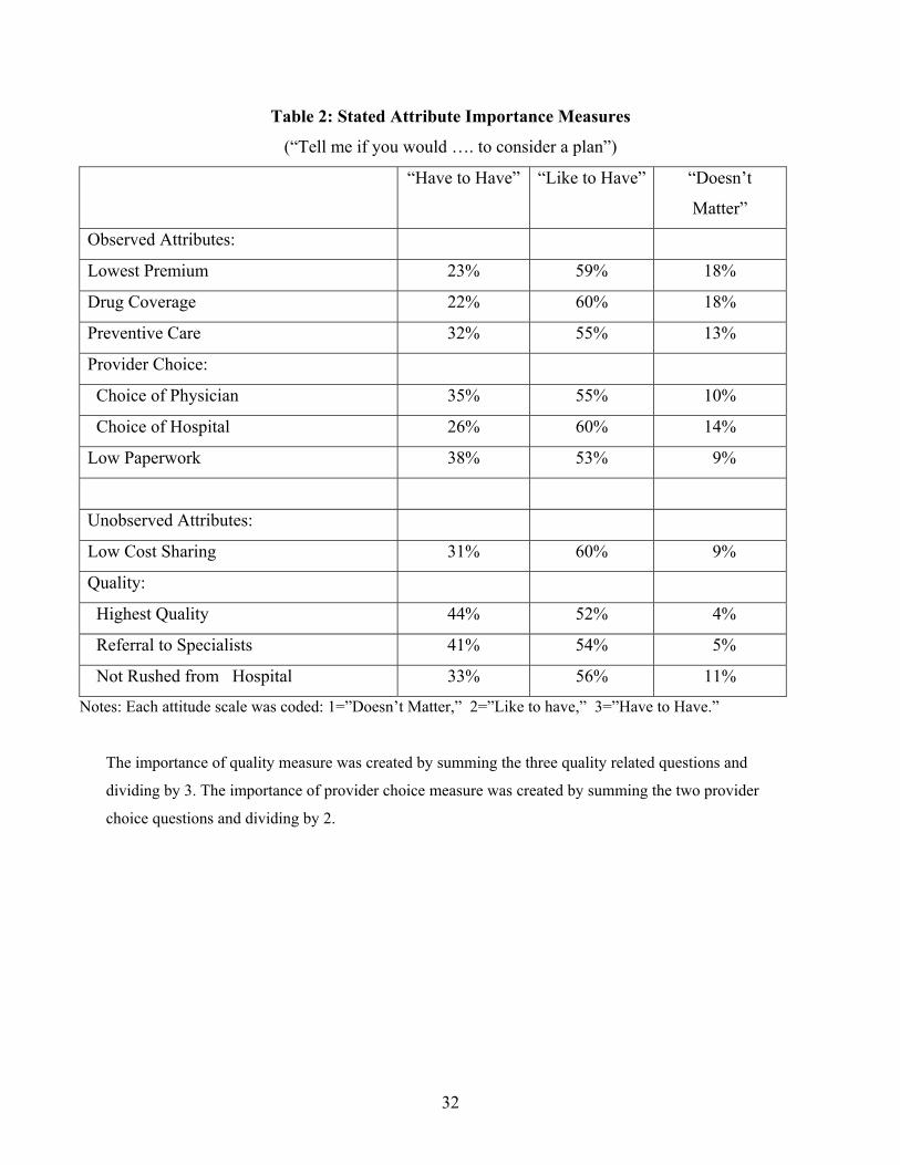
32

Table 2: Stated Attribute Importance Measures

(“Tell me if you would …. to consider a plan”)

“Have to Have” “Like to Have” “Doesn’t

Matter”

Observed Attributes:

Lowest Premium 23% 59% 18%

Drug Coverage 22% 60% 18%

Preventive Care 32% 55% 13%

Provider Choice:

Choice of Physician 35% 55% 10%

Choice of Hospital 26% 60% 14%

Low Paperwork 38% 53% 9%

Unobserved Attributes:

Low Cost Sharing 31% 60% 9%

Quality:

Highest Quality 44% 52% 4%

Referral to Specialists 41% 54% 5%

Not Rushed from Hospital 33% 56% 11%

Notes: Each attitude scale was coded: 1=”Doesn’t Matter,” 2=”Like to have,” 3=”Have to Have.”

The importance of quality measure was created by summing the three quality related questions and

dividing by 3. The importance of provider choice measure was created by summing the two provider

choice questions and dividing by 2.

33

Table 3: Parameter Estimates, Observed Attributes

Observed Attribute: Intercept Slope

Premium .014

(.011)

-.007**

(.003)

Drug Coverage .057

(.912)

.384**

(.145)

Preventive Care and No

Claims

1.887**

(.498)

.766**

(.202)

Provider Choice -.395

(1.081)

1.430**

(.489)

Must Submit Claims Collinear with Preventive

Care (Plans with preventive

care do not have claims)

-.274**

(.130)

Note: The “slope” coefficient must be multiplied by the stated importance weight Si = 1, 2, or 3, and the

result then added to the intercept to obtain the predicted importance weight for person i. Standard errors

are in parenthesis below the estimates. A “**” indicates significance at the 5% level.

34

Table 4: Predicted Utility Weight on “Drug Coverage”

for Different Levels of Stated Importance

S=1

“Doesn’t Matter”

S=2

“Like to Have”

S=3

“Have to Have”

.057+(1)·(.384)

= .441

.057+(2)·(.384)

= .825

.057+(3)·(.384)

= 1.209

35

Table 5: Parameter Estimates, Unobserved Attributes

Un-Observed Attribute Importance:

Estimates of Equation (3):

Wip = 2.688 · Sip* + υip p=1 (cost share), 2 (quality)

Estimates of the Un-observed attribute levels for each insurance plan

Un-observed (or “Latent”) attribute 1:

Cost Sharing Relative to Basic Medicare

Basic Medicare A11 0

Medigap without Drug Coverage A21 -.270

Medigap with Drug Coverage A31 -.355

IPA type HMO A41 -.414

Group HMO A51 -.271

Un-observed (or “Latent”) attribute 2:

Quality of Care Relative to Basic Medicare

Basic Medicare A12 0

Medigap without Drug Coverage A22 .269

Medigap with Drug Coverage A32 .261

IPA type HMO A42 -.081

Group HMO A52 .161

Note: The unobserved attribute levels for Basic Medicare are normalized to 0 since it is the base

alternative. Attribute levels for the other plans are measured relative to Basic Medicare. In equation (3),

Sip* is the weight (from 1 to 3) that person i says he/she puts on attribute p, and υip is “measurement

error.”

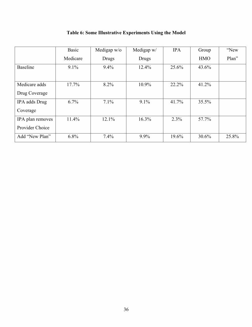
36

Table 6: Some Illustrative Experiments Using the Model

Basic

Medicare

Medigap w/o

Drugs

Medigap w/

Drugs

IPA Group

HMO

“New

Plan”

Baseline

9.1% 9.4% 12.4% 25.6% 43.6%

Medicare adds

Drug Coverage

17.7% 8.2% 10.9% 22.2% 41.2%

IPA adds Drug

Coverage

6.7% 7.1% 9.1% 41.7% 35.5%

IPA plan removes

Provider Choice

11.4% 12.1% 16.3% 2.3% 57.7%

Add “New Plan” 6.8% 7.4% 9.9% 19.6% 30.6% 25.8%