Mutual Funds in Equilibrium∗

Jonathan B. Berk† Jules H. van Binsbergen‡

February 16, 2017

Comments welcome

Abstract

Historically, the literature on money management has not consistently applied the

rational expectations equilibrium concept. We explain why and summarize recent

developments in the money management literature that do apply this concept correctly.

We demonstrate that in many respects the rational expectations equilibrium better

approximates the observed equilibrium in the money management space than it does in

the stock market. Moreover, many of the puzzles that have plagued the earlier literature

result from failing to apply the equilibrium concept correctly. Recent work reveals that

there is little support for the common conclusion that, as a group, investors in the

money management space are naive and that mutual fund managers are charlatans.

Even today, equilibrium thinking is not nearly as prevalent in mutual fund research as

it is in the rest of asset pricing. This state of play provides a multitude of opportunities

for future research in the area.

∗This article reflects our view of the recent advances in the mutual fund literature and is not intendedto be an impartial review of that literature. For discussions over the years, we thank Anat Admati, PeterDeMarzo, Darrell Duffie, Vincent Glode, Marco Grotteria, Binying Liu, Christian Opp, Lubos Pastor, PaulPfleiderer, Rob Stambaugh and Richard Stanton. We dedicate this article to Rick Green, who left us tooearly.†Stanford University, Graduate School of Business and NBER; jbberk@stanford.edu.‡Wharton, University of Pennsylvania and NBER; julesv@wharton.upenn.edu.

1. Introduction

The introduction of the rational expectations equilibrium framework was one of the key

intellectual insights that has defined modern financial economics. The idea that the price of

a stock adjusts to ensure the expected excess return of the stock (i.e. the expected return in

excess of the risk free rate) is solely a function of its risk, dominates how the field teaches and

thinks about stock prices and returns. Often termed the “efficient market hypothesis,” this

idea is commonplace in the finance literature today. In fact, one would be hard-pressed to find

a financial economist who does not appreciate the implication of the rational expectations

assumption on the behavior of stock prices.

In this article, we evaluate the state of the investment management literature by assessing

to what degree the same equilibrium thinking has penetrated that literature. What we

will show is that, until recently, the penetration was slight. Not correctly applying the

rational expectations paradigm has been costly. For years this literature has been caught in

a quagmire of seemingly contradictory results. Much of this confusion persists even today.

Until recently, many financial economists maintained a rather schizophrenic view of in-

vestors. When investors invest directly in stocks, the widely accepted view is that the ra-

tional expectations equilibrium so closely approximates the actual equilibrium, that changes

in stock prices in reaction to news can be used as evidence in a court of law as a measure

of the value of that news. On the other hand, when investors invest indirectly in stocks

through mutual funds, the generally accepted view was that in this market, investors are

naive. Consequently, according to this view, they choose to invest almost exclusively in neg-

ative net present value investments (Malkiel 1995, Carhart 1997, Fama and French 2010).

Furthermore, investor naivete is so dominant that the market does not equilibrate and so

returns reflect things other than risk, in particular, returns reflect managerial skill (or lack

thereof). Moreover, because fund flows into mutual funds are known to be highly predictable

based on past performance, but past performance has little or no predictability for future

performance, researchers concluded that mutual fund investors acted on information that

was worthless, what the literature has named “return chasing.” What is particularly per-

plexing about this dichotomous view of investors is that there is substantial overlap in the

investors in both markets.

In the last 10 years many of these apparent puzzles in the money management literature

have been resolved by applying the rational expectations equilibrium concept consistently in

the two markets (Berk and Green 2004, Berk and van Binsbergen 2015). In this article we

will review these developments and we will show that in many respects the rational expecta-

tions equilibrium better approximates the observed equilibrium in the money management

2

space than it does in the stock market. Moreover, we will show that the prior conclusions,

that investors in the money management space are entirely naive and that mutual fund

managers are all charlatans is incorrect and results from inconsistently applying the rational

expectations equilibrium concept. When the concept is applied correctly, empirical tests

reveal that there is in fact little support for either conclusion.

2. Background

There is a close relationship between how the rational expectations paradigm came to dom-

inate the way financial economists think about stock returns and how they thought about

money management returns. For this reason, we begin by briefly reviewing the history of

how the paradigm developed.

Although the equilibrium concept was first proposed by John Muth (Muth 1961), it was

popularized in financial economics in a series of articles authored by Eugene Fama (Fama

1965, Fama 1970, Fama 1976), and became known as the “efficient market hypothesis.” An

important, and much emphasized, implication of the rational expectations equilibrium is

that in such an equilibrium, the quality of a firm’s actions and decisions cannot be measured

by the expected return subsequent to the action or decision. Because investors compete

with each other for attractive investment opportunities, the price of the attractive stocks

(and bonds) is bid up to reflect the successfulness of the firm. That is, investors reward a

successful firm with a high market capitalization, not a high expected return going forward.

Instead of debating the theoretical point, the literature quickly shifted to empirically

testing whether or not in the data it is possible to find deviations from the rational expec-

tations equilibrium. While there is little consensus in the literature as to whether or not

prices reflect all (publicly) available information, there is widespread agreement that at a

minimum, prices reveal a substantial fraction of the information, making the cross-sectional

distribution of firm size (as measured by market capitalization) a much better measure of

firms’ success than the cross sectional distribution of subsequent returns. The extent to

which this idea has become widely accepted can be gauged by the fact that the change in

value of a company upon the release of public information is admissible in a court of law as

evidence of the value of the information itself. Put differently, it is widely accepted today

that the main implication of the rational expectations paradigm is that the impact of infor-

mation on a firm is measured by the change in value that results instantaneously when the

information is released, and not by the expected returns going forward after the information

is released.

Although the rational expectations paradigm came to dominate the pricing of financial

3

assets, it had little influence on the pricing of a closely related financial product, the mutual

fund. In that literature, exactly the opposite paradigm prevailed. In analyzing the behavior

of mutual funds, researchers ignored the total size of the fund and instead used the future

realized return as the measure of the quality of the fund. The two paradigms have radically

different predictions, and so the conclusions of the literatures about the value of informa-

tion were radically different. Stock price reactions were viewed as highly informative while

changes in mutual fund sizes were deemed random and uninformative. Because mutual fund

investors caused these “random” changes by responding to returns, they were deemed naive

return chasers. In addition, researchers found that, on average, mutual funds did not deliver

extra returns to their investors, i.e. there was no outperformance, which was interpreted

as implying that there was no information in mutual fund returns, leading to the widely

accepted perception that mutual fund managers lacked skill.

Before we examine the implications of consistently applying the rational expectations

paradigm to both kinds of financial products, it is worthwhile considering why financial

economists schizophrenically applied different concepts to two closely related investment

products. We believe the answer lies in the original work that argued for using the rational

expectations equilibrium concept to price stocks (Fama 1965, Malkiel 1995). In arguing for

the rational expectations paradigm, researchers took the position that stock prices impound

all information. Under this assumption, no agent should be able to predict future perfor-

mance, and so no agent should be able to make money picking stocks. To demonstrate the

empirical validity of this position, they used the performance of mutual funds. They argued

that because mutual funds did not deliver positive net alpha to their investors, mutual fund

managers lacked stock picking skill. The implication they drew from this evidence was that

if even the professionals who claimed to have the ability to pick stocks could not, stock

prices must indeed impound all information. However, this argument uses the rational ex-

pectations paradigm inconsistently. By assuming that the rational expectations equilibrium

described stock markets but not the equilibrium in money management, these researchers

used the net alpha to measure stock picking ability and thus incorrectly concluded that there

was no value to additional information other than what was already impounded in prices.

Once this inconsistency was put in place, it perpetuated, resulting in financial economists

inconsistently applying the paradigm in the two literatures.

Just as in stock markets, in mutual funds, investors also compete for attractive invest-

ment opportunities. In this case, the attractive investment opportunities are skilled fund

managers (rather than skilled firm managers) and the information of relevance is the degree

to which mutual fund managers can successfully pick stocks. There is, however, an impor-

tant difference between the two markets. Unlike stock markets, in the money management

4

market the price is fixed. That is, regardless of how skilled the manager who manages the

fund is, when an investor invests in a mutual fund, the price the investor pays for the fund is

always the market value of the fund’s underlying assets. What this implies is that the mar-

ket does not equilibrate through prices, it equilibrates in quantities (i.e. fund size). Other

than that difference, the rational expectations equilibrium in the two markets have identical

implications. The size of the fund measures the quality of the manager, the expected return

of the fund measures its risk.

To understand how the mutual fund market equilibrates, take a manager that delivers

positive average risk adjusted returns (net alphas) to investors. Investors soon find out about

this manager and compete for that extra return by showering the manager with additional

money. The size of the fund thus increases and because the manager’s investment ideas are

finite, eventually the additional money cannot be put to productive use. This lowers the

return the manager makes until investors no longer receive an extra return (i.e. the net alpha

falls to zero). At this point the flows will stop because investors no longer face an attractive

investment opportunity.

In the rational expectations equilibrium, competition between investors ensures that the

expected risk-adjusted excess return to investors (the net alpha) is zero, implying that it no

more measures the quality of a mutual fund manager than the expected return of a stock

measures the quality of a firm manager. For stocks, the equilibrium is reached by bidding up

the price of a successful firm thereby lowering the expected return to its equilibrium level,

whereas for mutual funds, the equilibrium is reached by increasing the size of the fund. As is

the case for stocks, the cross-sectional distribution of mutual fund success is predominantly

reflected in the cross-sectional distribution of fund size as opposed to the distribution of risk

adjusted excess returns to investors (net alpha). Just as with stocks, more skilled managers

manage larger funds, less skilled managers manage (very) small funds, and they all make

comparable net alphas close to zero.

In stock markets the rational expectations paradigm is often tested by assessing the extent

to which future returns are predictable given a news announcement. This predictability

provides evidence of the competitiveness of stock markets, and the rationality of investors.

Nobody argues that it is informative about the quality of firm management. The same logic

applies in the mutual fund space. If net alphas are not zero, we learn something about the

rational expectations of investors and the competition they face.

Theory models in economics are particularly useful if they can match moments in the

data that they were not designed to explain. Rational expectation models in mutual funds

have performed remarkably well in this regard, producing several predictions that the baseline

5

model (Berk and Green 2004) was not calibrated to. For example, the equilibrium arguments

in Berk and Green (2004) can be successfully employed to explain the behavior of closed-end

funds (Berk and Stanton 2007) and to understand the role of firms in the mutual fund space

(Berk, van Binsbergen, and Liu 2017). Finally, the insight has been successfully applied to

infer which risk model investors are using. Berk and van Binsbergen (2016) and Barber,

Huang, and Odean (2016) find, using mutual fund data, that the CAPM best explains

investor behavior and Blocher and Molyboga (2016) confirm these findings using hedge fund

data.

3. The Rational Expectations Equilibirum

Consider the following simple model of mutual fund management (Berk and Green 2004).

Let us start with a mutual fund manager who can generate a gross alpha (the alpha before

fees have been taken out) that depends on the amount of invested capital equal to:

(1) αg(q) = a− bq.

In words: the manager extracts from financial markets an extra amount a on the first cent

she manages. Because the manager’s investment ideas are in finite supply and because

she invests her best ideas first, the extra amount decreases at a rate b for every additional

dollar the manager invests.1 The total dollar amount this manager extracts from financial

markets, what we term the value added, is the product of the gross alpha and assets under

management:

(2) V (q) ≡ qαg(q) = q(a− bq).

If we assume that the manager’s objective is to maximize value added, then the optimal

amount to invest maximizes this quadratic function. Taking first order conditions with

respect to q and setting this equal to zero gives

(3) q∗ =a

2b,

implying that gross alpha at the optimum is

(4) αg(q∗) =a

2.

1For ease of exposition we assume that the gross alpha is a linear function of fund size q, but the argumentspresented do not rely on this linearity.

6

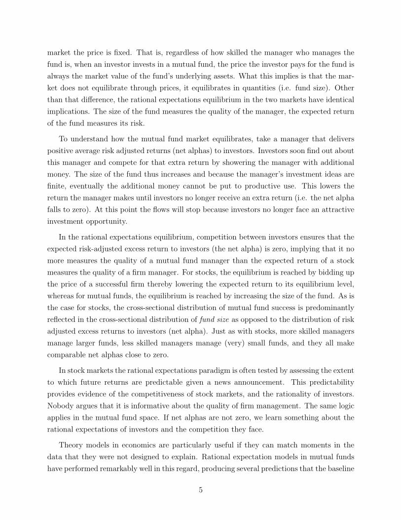
The value added at the maximum is given by:

(5) V ∗ =a2

4b.

Figure 1 plots the value added (V) and gross alpha (αg) as a function of q. The figure also

shows the value added and gross alpha at the optimal amount of money. Before we consider

Figure 1: Size, Value Added and Gross AlphaThe graph shows the relationship between size and value added/gross alpha.

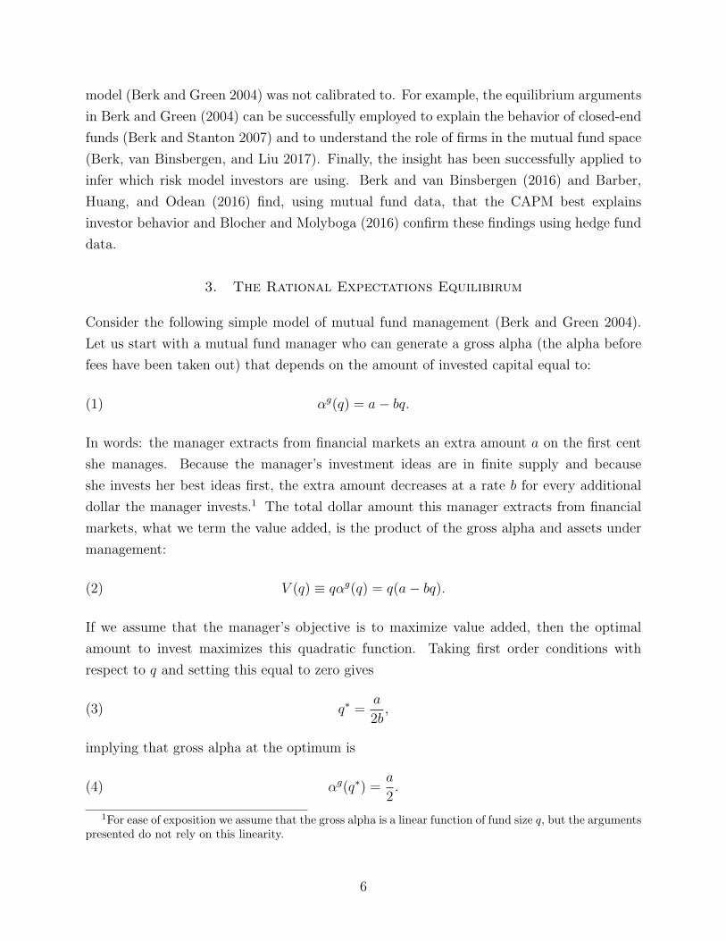
the investor’s problem, it is worth comparing this manager to a manager of lower quality.

Consider manager 2. Manager 2 runs out of good ideas more quickly than manager 1. That

is, while manager 2 makes the same extra return on the first cent (equal to a), the rate at

which the return deteriorates is twice as large and equal to 2b instead of b. In Figure 2 we

plot the gross alpha of both managers as well as their value added. The optimal investment

amount for manager 2 is twice as small as that for manager 1 and equal to a/4b. Because

the gross alpha at the optimum is independent of the parameter b, both managers have the

same gross alpha equal to a/2 at the optimum. Hence, gross alpha is not correlated with

skill. If one were to use gross alpha as a measure of skill, we would come to the (wrong)

conclusion that both managers are equally skilled. This result follows only from the fact

7

that, if there are decreasing returns to scale, returns are not a good measure of (or proxy

for) value and no assumptions related to rational expectations are required.

Figure 2: Size, Value Added and Gross AlphaThe graph shows the relationship between size and value added/gross alpha for two managers. Manager 1 ismore skilled than Manager 2 while both make the same gross alpha on the first cent they invest. Manager 1has an investment strategy that is more scalable than Manager 2. That is, manager 2’s decreasing returnsto scale parameter (b) is higher than manager 1’s.

We now turn to investors and assume that they have rational expectations. A rational

investor will chase any positive net present value investment opportunity. This implies that

all assets earn an expected return commensurate with the risk of the asset. As a consequence,

all funds must have net alphas of zero. If the manager picks her fee, f , equal to

f =a

2,

investors will choose to invest q∗ = a2b

in the fund. As a consequence the fund’s net alpha

will be zero and the market will be in equilibrium. In the case of the second manager, the

fee will be the same, but in this case the equilibrium investment is a4b

. That is, although

both managers have the same gross (and net) alpha, manager 1 has twice as much money in

equilibrium as manager 2. The total amount of money manager 1 extracts from markets is

8

V ∗ = αg(q∗)q∗ = a2× a

2b= a2

4bwhich is twice the amount that manager 2 extracts, a

2× a

4b= a2

8b,

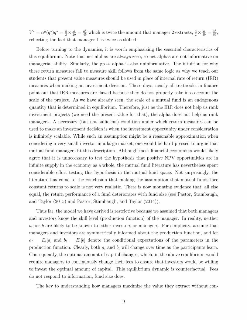
reflecting the fact that manager 1 is twice as skilled.

Before turning to the dynamics, it is worth emphasizing the essential characteristics of

this equilibrium. Note that net alphas are always zero, so net alphas are not informative on

managerial ability. Similarly, the gross alpha is also uninformative. The intuition for why

these return measures fail to measure skill follows from the same logic as why we teach our

students that present value measures should be used in place of internal rate of return (IRR)

measures when making an investment decision. These days, nearly all textbooks in finance

point out that IRR measures are flawed because they do not properly take into account the

scale of the project. As we have already seen, the scale of a mutual fund is an endogenous

quantity that is determined in equilibrium. Therefore, just as the IRR does not help us rank

investment projects (we need the present value for that), the alpha does not help us rank

managers. A necessary (but not sufficient) condition under which return measures can be

used to make an investment decision is when the investment opportunity under consideration

is infinitely scalable. While such an assumption might be a reasonable approximation when

considering a very small investor in a large market, one would be hard pressed to argue that

mutual fund managers fit this description. Although most financial economists would likely

agree that it is unnecessary to test the hypothesis that positive NPV opportunities are in

infinite supply in the economy as a whole, the mutual fund literature has nevertheless spent

considerable effort testing this hypothesis in the mutual fund space. Not surprisingly, the

literature has come to the conclusion that making the assumption that mutual funds face

constant returns to scale is not very realistic. There is now mounting evidence that, all else

equal, the return performance of a fund deteriorates with fund size (see Pastor, Stambaugh,

and Taylor (2015) and Pastor, Stambaugh, and Taylor (2014)).

Thus far, the model we have derived is restrictive because we assumed that both managers

and investors know the skill level (production function) of the manager. In reality, neither

a nor b are likely to be known to either investors or managers. For simplicity, assume that

managers and investors are symmetrically informed about the production function, and let

at = Et[a] and bt = Et[b] denote the conditional expectations of the parameters in the

production function. Clearly, both at and bt will change over time as the participants learn.

Consequently, the optimal amount of capital changes, which, in the above equilibrium would

require managers to continuously change their fees to ensure that investors would be willing

to invest the optimal amount of capital. This equilibrium dynamic is counterfactual. Fees

do not respond to information, fund size does.

The key to understanding how managers maximize the value they extract without con-

9

tinuously adjusting their fees is to consider the manager’s problem. Notice that from the

manager’s perspective, it is always suboptimal to invest anything other than q∗ in active

management. Consequently, he will continue to invest this amount, regardless of the fee,

by either borrowing money (if possible) when the fee is too high and so investors choose

to invest less than q∗, or indexing the excess money when the fee is too low and investors

provide more capital than q∗.

Let us explicitly consider the second case. Suppose that the fund size at time t, qt is

larger than q∗t = at

2btbecause f < at

2. The optimal strategy for the manager is to put q∗t into

active management and index the difference, qt − q∗t . In this case, the indexed money earns

no alpha, so the equilibrium gross alpha on the whole fund is given by:

(6)

(q∗tqt

)at

2+

(qt − q∗

qt

)0 =

a2t

4qtbt.

In equilibrium, the net alpha of the fund must be zero. Imposing this restriction gives

(7)a2

t

4qtbt− f = 0.

The equilibrium size of the fund is thus:

(8) qt =a2

t

4fbt.

Notice that the dynamic equilibrium where fees are fixed, shares an important characteristic

with the static equilibrium: in both cases the gross alpha equals the fee charged, and therefore

is not a reliable measure of managerial skill. Given that the size of the fund adjusts to ensure

that the gross alpha and the fee are equal, it is not appropriate to think about gross alpha

and fund size as two independent entities. Because they are related in equilibrium, the size

of the fund and the gross alpha (i.e. the fee) are not separately identified by the parameters

that determine managerial skill. Their product, on the other hand, is uniquely identified by

those two parameters: regardless of the fee the manager chooses, the product of the size of

the fund (q) and the equilibrium gross alpha (the fee) equals:

(9) V ∗t =

a2t

4fbtf =

a2t

4qtbtqt =

a2t

4bt.

This product is what we call the value added of the fund. It is the correct way to measure

managerial skill because it measures the manager’s value added and is a function of only the

skill of the manager.

10

In summary, with indexing and fixed fees, fund size adjusts to ensure that the gross alpha

is sufficiently high to cover the manager’s fees. There is a wide range of fees that all allow the

manager to fully exploit her skill and extract the optimal amount of money from financial

markets. What this implies is that the fee charged is irrelevant — managers can choose to

charge a high fee and manage a small fund, or charge a low fee and manage a large fund.

In both cases the amount the manager makes as well as the return the investors earn, is the

same. Because gross alpha must equal the fee in equilibrium, it too is irrelevant.

This simple dynamic rational expectations equilibrium is able to explain the important

empirical regularities documented in the mutual fund literature, as well as resolve the most

important puzzles. Specifically, the fact that future return performance of the fund is un-

predictable follows directly from the rational expectations equilibrium requirement that net

alpha is always zero. Fund size, in this equilibrium, continuously adjusts in response to

information. One source of information is past returns, and so the equilibrium predicts that

the flow of funds responds to past performance. This flow-performance relation is not ev-

idence of investor suboptimality, quite the contrary. It is evidence of the competitiveness

with which investors chase positive net present value investment opportunities. As we have

already mentioned, the model also has new predictions about empirical moments (e.g. value

added) that were not identified at the time the model was derived. We will review the

empirical performance of the model using these moments in Section 6.

Finally, the equilibrium described above teaches another important lesson. Some have

argued that investment managers should be more generous to their investors by lowering

their fees thereby giving up a larger part of their performance to their investors. What the

equilibrium shows is that it is not the manager’s choice of fees that sets the return to investors

equal to zero. It is competition between investors for good investment opportunities. The

fee is irrelevant to this discussion. The only way a manager can be more generous to her

investors is if the manager stops accepting money from new investors, thereby favoring old

investors over new investors.

4. Measuring Mutual Fund Performance

Now that we have explained how the rational expectations equilibrium works in mutual funds,

we can turn to a central question in that literature – how is fund performance measured?

The answer to this question depends on what we mean by fund performance. Often, what

financial economists mean is the performance of investors in the fund, that is, how much

better off would the marginal investor be by investing an additional dollar in that fund.

In this case, the measure of performance is the fund’s net alpha. If, on the other hand,

11

the objective is to measure how skilled the fund manager is, then, as we have seen, alpha

measures are uninformative. To answer the skill question, we must use the correct measure

of fund performance: value added. The unfortunate fact is that until recently financial

economists have used alpha measures almost exclusively to measure managerial skill, and

in doing so, have reached the incorrect conclusion that managers are unskilled. As we will

demonstrate in Section 6, when the correct measure is used a different picture emerges.

It is important to understand that while under the rational expectations paradigm the

only measure of managerial skill is value added, value added always measures the amount

of money extracted from markets regardless of whether the rational expectations paradigm

holds. To understand why, notice that

Vt = qtαgt (qt) = qtα

nt (qt) + qtf

where αnt (qt) is the net alpha of the fund as a function of fund size. The first term in the

above equation is the amount of money the manager either gives to or takes from investors.

The second term is the amount of money the manager takes for himself. Notice that there

is no other source of funds. What this observation implies is that the money the manager

takes in compensation can only come from one of two places, either from skill (through stock

picking) or from investors (by underperforming). So the sum of these two terms must equal

the amount of money the manager makes from his stock picks. This observation relies on no

other assumption other than this budget constraint.

The fact that both the measure of investor performance (net-alpha) and the measure of

value extracted from financial markets do not depend on any further assumptions implies

that they are independent of whatever Null hypothesis is assumed. For example, a very

common Null in the mutual fund literature is that managers have no skill. To reject this

Null, one must show that value added is positive. Another interesting Null is that the

rational expectations equilibrium describes the behavior of mutual funds. To reject this Null

one would need to show that the net alpha of the fund is nonzero. Finally, one could also

test the Null that the mutual fund market is perfectly competitive, so all positive net present

value investment opportunities are competed away. To reject this Null one would need to

show that the net alpha was positive. In summary then, the net alpha is informative about

investor rationality and the degree of competition in markets. Value added is informative

about the skill level of fund managers.

12

5. Benchmarks

The Achilles heel of the mutual fund literature is how to construct a manager’s counterfactual

performance absent any skill. Generally two methods have been applied. The standard prac-

tice in financial economics is not to construct the alternative investment opportunity itself,

but rather to simply adjust for risk using a risk model. In recent years, the extent to which

risk models accurately correct for risk has been subject to extensive debate. In response to

this, mutual fund researchers have opted to construct the alternative investment opportunity

directly. Although in principle this approach is a sensible way to address the issue of not

knowing the correct model of risk, the way this approach is typically implemented in practice

replaces one shortcoming with another. What researchers have typically done is assume that

investors’ next best investment opportunities are spanned by the factor mimicking portfo-

lios in the Fama-French-Carhart factor specification (Fama and French 1996, Carhart 1997).

That is, they have interpreted the factor mimicking portfolios in these factor specifications

as investment opportunities available to investors, rather than risk factors.

There are two reasons why these factor portfolios are not investable opportunities. The

first is straightforward. These portfolios do not include transaction costs. In essence, you

cannot compare the performance of a fund that incurs transaction costs to a fund that does

not. The second issue is more subtle. The factors that are typically used were identified in the

the late 1980’s and 1990’s and popularized by Fama and French (1996) and Carhart (1997).

However, most studies include data that begin at least 20 years before those factors were

identified. In those earlier years, investors would not have known about these portfolios

and obviously could not have invested in them. By using these portfolios to benchmark

managers, researchers are effectively evaluating managers in 1970 using 1990’s technology.

Any manager who, in 1970, knew about the investment opportunities afforded by these

portfolios should be given credit for this knowledge and the subsequent outperformance.

By benchmarking managers against non-investable benchmarks, researchers are effec-

tively handicapping managers. To estimate the size of this handicap, we can evaluate the

“performance” of the factor portfolios themselves against a set of passive, but investable,

benchmarks. The most obvious set to use is the set of index funds offered by the Vanguard

company. The advantage of using these funds is that they are constructed for the purpose

of giving investors the least costly method to diversification. This explicit objective is not

shared by alternative benchmarks constructed by companies such as Morningstar. More-

over, Vanguard is not only the market leader offering this service, it is also the pioneer in

the space. For example, the 11 funds listed in Table 1 span the set of all index funds offered

by the firm. In each case, the Vanguard fund was the first index fund to offer that particular

13

strategy. That means that these funds are natural indicators to use to determine when a

strategy becomes widely known to all investors.

It is not uncommon in the mutual fund literature to use style benchmarks that are either

identified by the fund itself or by external organizations such as Morningstar. The problem

with using these benchmarks is that many funds regularly deviate from the style objectives

they report and advertise. By simply projecting each fund on all available Vanguard index

funds, such potential misclassifications are avoided.

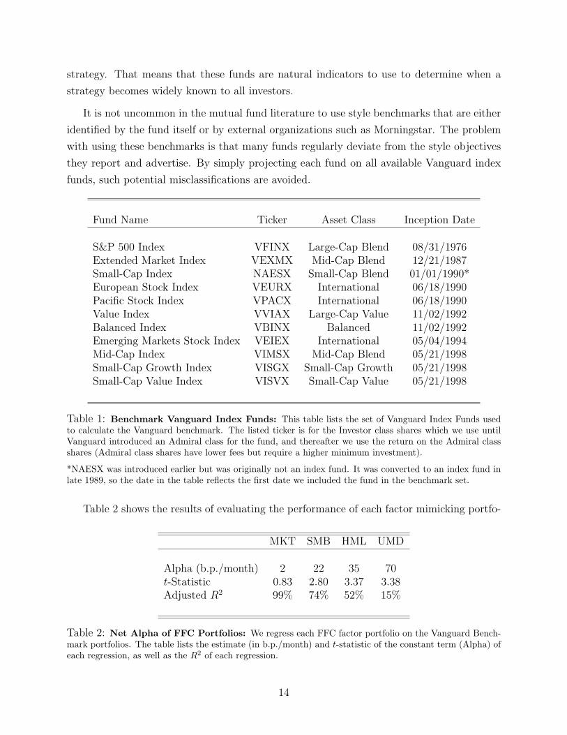
Fund Name Ticker Asset Class Inception Date

S&P 500 Index VFINX Large-Cap Blend 08/31/1976Extended Market Index VEXMX Mid-Cap Blend 12/21/1987Small-Cap Index NAESX Small-Cap Blend 01/01/1990*European Stock Index VEURX International 06/18/1990Pacific Stock Index VPACX International 06/18/1990Value Index VVIAX Large-Cap Value 11/02/1992Balanced Index VBINX Balanced 11/02/1992Emerging Markets Stock Index VEIEX International 05/04/1994Mid-Cap Index VIMSX Mid-Cap Blend 05/21/1998Small-Cap Growth Index VISGX Small-Cap Growth 05/21/1998Small-Cap Value Index VISVX Small-Cap Value 05/21/1998

Table 1: Benchmark Vanguard Index Funds: This table lists the set of Vanguard Index Funds usedto calculate the Vanguard benchmark. The listed ticker is for the Investor class shares which we use untilVanguard introduced an Admiral class for the fund, and thereafter we use the return on the Admiral classshares (Admiral class shares have lower fees but require a higher minimum investment).

*NAESX was introduced earlier but was originally not an index fund. It was converted to an index fund inlate 1989, so the date in the table reflects the first date we included the fund in the benchmark set.

Table 2 shows the results of evaluating the performance of each factor mimicking portfo-

MKT SMB HML UMD

Alpha (b.p./month) 2 22 35 70t-Statistic 0.83 2.80 3.37 3.38Adjusted R2 99% 74% 52% 15%

Table 2: Net Alpha of FFC Portfolios: We regress each FFC factor portfolio on the Vanguard Bench-mark portfolios. The table lists the estimate (in b.p./month) and t-statistic of the constant term (Alpha) ofeach regression, as well as the R2 of each regression.

14

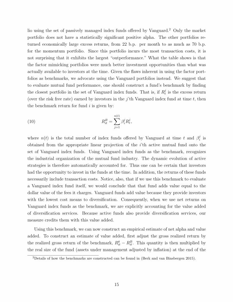
lio using the set of passively managed index funds offered by Vanguard.2 Only the market

portfolio does not have a statistically significant positive alpha. The other portfolios re-

turned economically large excess returns, from 22 b.p. per month to as much as 70 b.p.

for the momentum portfolio. Since this portfolio incurs the most transaction costs, it is

not surprising that it exhibits the largest “outperformance.” What the table shows is that

the factor mimicking portfolios were much better investment opportunities than what was

actually available to investors at the time. Given the flaws inherent in using the factor port-

folios as benchmarks, we advocate using the Vanguard portfolios instead. We suggest that

to evaluate mutual fund performance, one should construct a fund’s benchmark by finding

the closest portfolio in the set of Vanguard index funds. That is, if Rjt is the excess return

(over the risk free rate) earned by investors in the j’th Vanguard index fund at time t, then

the benchmark return for fund i is given by:

(10) RBit =

n(t)∑j=1

βjiR

jt ,

where n(t) is the total number of index funds offered by Vanguard at time t and βji is

obtained from the appropriate linear projection of the i’th active mutual fund onto the

set of Vanguard index funds. Using Vanguard index funds as the benchmark, recognizes

the industrial organization of the mutual fund industry. The dynamic evolution of active

strategies is therefore automatically accounted for. Thus one can be certain that investors

had the opportunity to invest in the funds at the time. In addition, the returns of these funds

necessarily include transaction costs. Notice, also, that if we use this benchmark to evaluate

a Vanguard index fund itself, we would conclude that that fund adds value equal to the

dollar value of the fees it charges. Vanguard funds add value because they provide investors

with the lowest cost means to diversification. Consequently, when we use net returns on

Vanguard index funds as the benchmark, we are explicitly accounting for the value added

of diversification services. Because active funds also provide diversification services, our

measure credits them with this value added.

Using this benchmark, we can now construct an empirical estimate of net alpha and value

added. To construct an estimate of value added, first adjust the gross realized return by

the realized gross return of the benchmark, Rgit − RB

it . This quantity is then multiplied by

the real size of the fund (assets under management adjusted by inflation) at the end of the

2Details of how the benchmarks are constructed can be found in (Berk and van Binsbergen 2015).

15

previous period, qi,t−1, to obtain the realized value added between times t− 1 and t:

(11) Vit ≡ qi,t−1

(Rg

it −RBit

).

The time series average of Vit measures a fund’s value added. Similarly, if Rnit is the return

investors in the fund earn (i.e., the return after all fees are taken out), then define

(12) εit ≡ Rnit −RB

it .

The time series average of εit is an estimate of the fund’s net alpha.

6. Managerial Skill

We begin describing the results reported in Berk and van Binsbergen (2015). That paper

measures the average value added of mutual fund managers over the period 1977-2011 in

January 1, 2000 dollars.3 The results are reported in Table 3. The paper finds that mutual

fund managers are skilled. The average fund adds an economically significant $140,000 per

month (in Y2000 dollars). There is also large variation across funds. The fund at the 99th

percentile cutoff generated $7.82 million per month and the fund at the 90th percentile cutoff

generated $750,000 a month on average. The median fund lost an average of $20,000/month,

and only 43% of funds had positive estimated value added. The main insight is that most

managers destroyed value but because most of the capital is controlled by skilled managers,

as a group, active mutual funds added considerable value.

Successful funds are more likely to survive than unsuccessful funds. Consequently, one

can think about the average value added of all mutual funds as estimates of the ex-ante

distribution of talent. We can also compute the average Vit in the data set without first

averaging by funds. Because surviving funds are overrepresented in this mean, we obtain

an estimate of the ex-post distribution of talent, that is, the average skill of the set of funds

actually managing money. Not surprisingly this estimate is higher. The average fund added

$270,000/month.

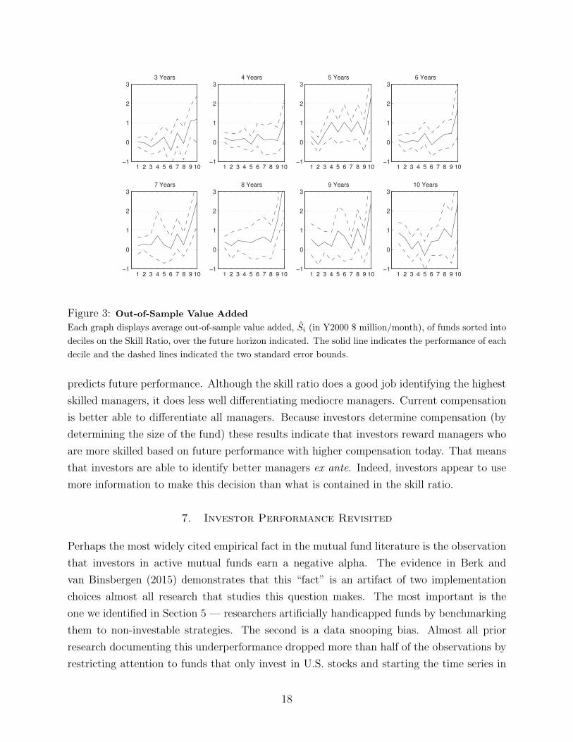
The paper also shows that managerial skill is persistent. It demonstrates this by first

sorting funds into deciles using the skill ratio — the estimated value of a fund’s value added

divided by its standard error. The skill ratio at any point in time is essentially the t-static

of the value added estimate measured over the entire history of the fund until that time.

Funds in the 10th (top) decile are the funds where we have the most confidence that the

3The data is available from 1962, but the analysis begins in 1977 because that is the year Vanguardoffered its first index fund.

16

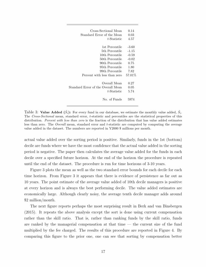
Cross-Sectional Mean 0.14Standard Error of the Mean 0.03

t-Statistic 4.57

1st Percentile -3.605th Percentile -1.15

10th Percentile -0.5950th Percentile -0.0290th Percentile 0.7595th Percentile 1.8099th Percentile 7.82

Percent with less than zero 57.01%

Overall Mean 0.27Standard Error of the Overall Mean 0.05

t-Statistic 5.74

No. of Funds 5974

Table 3: Value Added (Si): For every fund in our database, we estimate the monthly value added, Si.The Cross-Sectional mean, standard error, t-statistic and percentiles are the statistical properties of thisdistribution. Percent with less than zero is the fraction of the distribution that has value added estimatesless than zero. The Overall mean, standard error and t-statistic are computed by computing the averagevalue added in the dataset. The numbers are reported in Y2000 $ millions per month.

actual value added over the sorting period is positive. Similarly, funds in the 1st (bottom)

decile are funds where we have the most confidence that the actual value added in the sorting

period is negative. The paper then calculates the average value added for the funds in each

decile over a specified future horizon. At the end of the horizon the procedure is repeated

until the end of the dataset. The procedure is run for time horizons of 3-10 years.

Figure 3 plots the mean as well as the two standard error bounds for each decile for each

time horizon. From Figure 3 it appears that there is evidence of persistence as far out as

10 years. The point estimate of the average value added of 10th decile managers is positive

at every horizon and is always the best performing decile. The value added estimates are

economically large. Although clearly noisy, the average tenth decile manager adds around

$2 million/month.

The next figure reports perhaps the most surprising result in Berk and van Binsbergen

(2015). It repeats the above analysis except the sort is done using current compensation

rather than the skill ratio. That is, rather than ranking funds by the skill ratio, funds

are ranked by the managerial compensation at that time — the current size of the fund

multiplied by the fee charged. The results of this procedure are reported in Figure 4. By

comparing this figure to the prior one, one can see that sorting by compensation better

17

1 2 3 4 5 6 7 8 9 10−1

0

1

2

3

3 Years

1 2 3 4 5 6 7 8 9 10−1

0

1

2

3

4 Years

1 2 3 4 5 6 7 8 9 10−1

0

1

2

3

5 Years

1 2 3 4 5 6 7 8 9 10−1

0

1

2

3

6 Years

1 2 3 4 5 6 7 8 9 10−1

0

1

2

3

7 Years

1 2 3 4 5 6 7 8 9 10−1

0

1

2

3

8 Years

1 2 3 4 5 6 7 8 9 10−1

0

1

2

3

9 Years

1 2 3 4 5 6 7 8 9 10−1

0

1

2

3

10 Years

Figure 3: Out-of-Sample Value AddedEach graph displays average out-of-sample value added, Si (in Y2000 $ million/month), of funds sorted intodeciles on the Skill Ratio, over the future horizon indicated. The solid line indicates the performance of eachdecile and the dashed lines indicated the two standard error bounds.

predicts future performance. Although the skill ratio does a good job identifying the highest

skilled managers, it does less well differentiating mediocre managers. Current compensation

is better able to differentiate all managers. Because investors determine compensation (by

determining the size of the fund) these results indicate that investors reward managers who

are more skilled based on future performance with higher compensation today. That means

that investors are able to identify better managers ex ante. Indeed, investors appear to use

more information to make this decision than what is contained in the skill ratio.

7. Investor Performance Revisited

Perhaps the most widely cited empirical fact in the mutual fund literature is the observation

that investors in active mutual funds earn a negative alpha. The evidence in Berk and

van Binsbergen (2015) demonstrates that this “fact” is an artifact of two implementation

choices almost all research that studies this question makes. The most important is the

one we identified in Section 5 — researchers artificially handicapped funds by benchmarking

them to non-investable strategies. The second is a data snooping bias. Almost all prior

research documenting this underperformance dropped more than half of the observations by

restricting attention to funds that only invest in U.S. stocks and starting the time series in

18

1 2 3 4 5 6 7 8 9 10−1

0

1

2

3

4

3 Years

1 2 3 4 5 6 7 8 9 10−1

0

1

2

3

4

4 Years

1 2 3 4 5 6 7 8 9 10−1

0

1

2

3

4

5 Years

1 2 3 4 5 6 7 8 9 10−1

0

1

2

3

4

6 Years

1 2 3 4 5 6 7 8 9 10−1

0

1

2

3

4

7 Years

1 2 3 4 5 6 7 8 9 10−1

0

1

2

3

4

8 Years

1 2 3 4 5 6 7 8 9 10−1

0

1

2

3

4

9 Years

1 2 3 4 5 6 7 8 9 10−1

0

1

2

3

4

10 Years

Figure 4: Value Added Sorted on CompensationEach graph displays average out-of-sample value added, Si (in Y2000 $ million/month), of funds sorted intodeciles based on total compensation (fees × AUM). The solid line indicates the performance of each decileand the dashed lines indicated the 95% confidence bands (two standard errors from the estimate).

the early eighties. We can think of no reason for this data selection procedure.

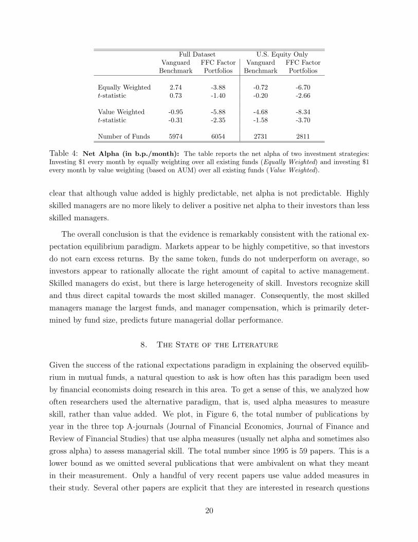
We begin by estimating the average net alpha by calculating the average εit across all

funds by equally and value weighting the funds. As Table 4 shows, over this time period

estimated net alpha is not statistically distinguishable from zero. For comparison purposes,

the table recalculates these estimates under the two implementation choices made by the

literature. Because the factor portfolios can be constructed in 1962, in this case we begin

the analysis in 1962. As one would expect, when funds are handicapped by requiring them

to outperform a non-investable benchmark, the net alpha estimate drops. If one then also

drops funds that do hold international stocks, the net alpha drops again. With both im-

plementation choices the net alpha estimate is indeed negative and statistically significantly

different from zero.

The evidence in Table 4 is consistent with the rational expectations equilibrium. But

importantly, that equilibrium imposes further restrictions. It requires that any realized

return in excess of the benchmark be unpredictable. Figure 5 repeats the persistence analysis

in the previous section but instead of reporting value added, it reports net alpha. That is,

at the beginning of each horizon, funds are sorted into deciles using the skill ratio and then

the weighted average εit of the decile over the horizon is calculated. From the figure it is

19

Full Dataset U.S. Equity OnlyVanguard FFC Factor Vanguard FFC Factor

Benchmark Portfolios Benchmark Portfolios

Equally Weighted 2.74 -3.88 -0.72 -6.70t-statistic 0.73 -1.40 -0.20 -2.66

Value Weighted -0.95 -5.88 -4.68 -8.34t-statistic -0.31 -2.35 -1.58 -3.70

Number of Funds 5974 6054 2731 2811

Table 4: Net Alpha (in b.p./month): The table reports the net alpha of two investment strategies:Investing $1 every month by equally weighting over all existing funds (Equally Weighted) and investing $1every month by value weighting (based on AUM) over all existing funds (Value Weighted).

clear that although value added is highly predictable, net alpha is not predictable. Highly

skilled managers are no more likely to deliver a positive net alpha to their investors than less

skilled managers.

The overall conclusion is that the evidence is remarkably consistent with the rational ex-

pectation equilibrium paradigm. Markets appear to be highly competitive, so that investors

do not earn excess returns. By the same token, funds do not underperform on average, so

investors appear to rationally allocate the right amount of capital to active management.

Skilled managers do exist, but there is large heterogeneity of skill. Investors recognize skill

and thus direct capital towards the most skilled manager. Consequently, the most skilled

managers manage the largest funds, and manager compensation, which is primarily deter-

mined by fund size, predicts future managerial dollar performance.

8. The State of the Literature

Given the success of the rational expectations paradigm in explaining the observed equilib-

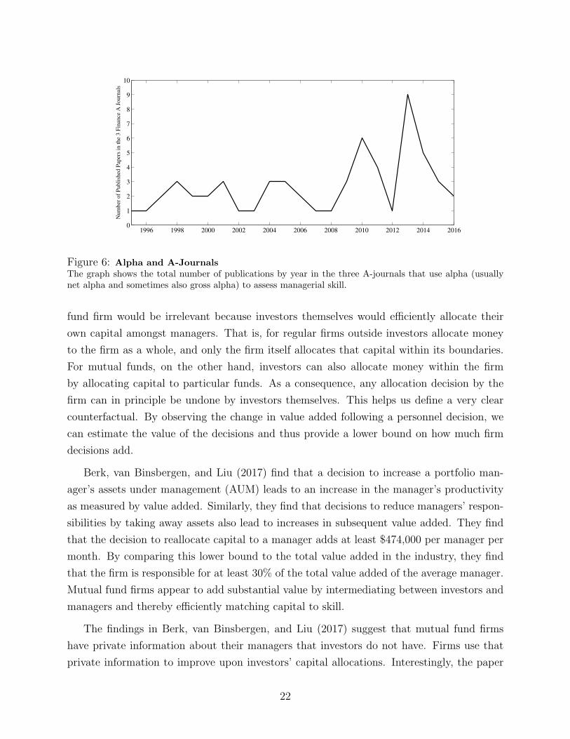
rium in mutual funds, a natural question to ask is how often has this paradigm been used

by financial economists doing research in this area. To get a sense of this, we analyzed how

often researchers used the alternative paradigm, that is, used alpha measures to measure

skill, rather than value added. We plot, in Figure 6, the total number of publications by

year in the three top A-journals (Journal of Financial Economics, Journal of Finance and

Review of Financial Studies) that use alpha measures (usually net alpha and sometimes also

gross alpha) to assess managerial skill. The total number since 1995 is 59 papers. This is a

lower bound as we omitted several publications that were ambivalent on what they meant

in their measurement. Only a handful of very recent papers use value added measures in

their study. Several other papers are explicit that they are interested in research questions

20

1 2 3 4 5 6 7 8 9 10−20

−15

−10

−5

0

5

10

3 Years

1 2 3 4 5 6 7 8 9 10−20

−15

−10

−5

0

5

10

4 Years

1 2 3 4 5 6 7 8 9 10−20

−15

−10

−5

0

5

10

5 Years

1 2 3 4 5 6 7 8 9 10−20

−15

−10

−5

0

5

10

6 Years

1 2 3 4 5 6 7 8 9 10−20

−15

−10

−5

0

5

10

7 Years

1 2 3 4 5 6 7 8 9 10−20

−15

−10

−5

0

5

10

8 Years

1 2 3 4 5 6 7 8 9 10−20

−15

−10

−5

0

5

10

9 Years

1 2 3 4 5 6 7 8 9 10−20

−15

−10

−5

0

5

10

10 Years

Figure 5: Out-of-Sample Net AlphaEach graph displays the out-of-sample performance (in b.p./month) of funds sorted into deciles on the SkillRatio over the horizon indicated. The solid line indicates the performance of each decile and the dashedlines indicated the 95% confidence bands (two standard errors from the estimate).

related to returns to investors. For those research questions, the net alpha is of course the

right measure to use.

9. Implications

The implication of the evidence presented in Sections 6 and 7 is that the same paradigm

explains the behavior of stock market investors and mutual fund investors. This insight

opens the opportunity for researchers to investigate questions, that traditionally have been

restricted to stock markets, in mutual fund markets. In this section we will illustrate the

potential gain to knowledge of following this approach by reviewing two articles that test

important economic questions using the mutual fund data base.

9.1. The Importance of Firms

A central question in corporate finance is why firms exist. The mutual fund industry is an

ideal place to study this question for several reasons. First, it is one of the few sectors in

the economy where employee productivity is observable. Thus, one can observe the change

in employee productivity that results from firm decisions. Second, in a world with perfectly

rational players, no information asymmetries and no other frictions, the role of a mutual

21

1996 1998 2000 2002 2004 2006 2008 2010 2012 2014 20160

1

2

3

4

5

6

7

8

9

10

Nu

mb

er o

f P

ub

lish

ed P

aper

s in

th

e 3

Fin

ance

A J

ou

rnal

s

Figure 6: Alpha and A-JournalsThe graph shows the total number of publications by year in the three A-journals that use alpha (usuallynet alpha and sometimes also gross alpha) to assess managerial skill.

fund firm would be irrelevant because investors themselves would efficiently allocate their

own capital amongst managers. That is, for regular firms outside investors allocate money

to the firm as a whole, and only the firm itself allocates that capital within its boundaries.

For mutual funds, on the other hand, investors can also allocate money within the firm

by allocating capital to particular funds. As a consequence, any allocation decision by the

firm can in principle be undone by investors themselves. This helps us define a very clear

counterfactual. By observing the change in value added following a personnel decision, we

can estimate the value of the decisions and thus provide a lower bound on how much firm

decisions add.

Berk, van Binsbergen, and Liu (2017) find that a decision to increase a portfolio man-

ager’s assets under management (AUM) leads to an increase in the manager’s productivity

as measured by value added. Similarly, they find that decisions to reduce managers’ respon-

sibilities by taking away assets also lead to increases in subsequent value added. They find

that the decision to reallocate capital to a manager adds at least $474,000 per manager per

month. By comparing this lower bound to the total value added in the industry, they find

that the firm is responsible for at least 30% of the total value added of the average manager.

Mutual fund firms appear to add substantial value by intermediating between investors and

managers and thereby efficiently matching capital to skill.

The findings in Berk, van Binsbergen, and Liu (2017) suggest that mutual fund firms

have private information about their managers that investors do not have. Firms use that

private information to improve upon investors’ capital allocations. Interestingly, the paper

22

finds that the value added of managers goes up after a demotion, suggesting that mutual

fund executives have a better knowledge of their manager’s ability than the managers them-

selves. This finding is consistent with our assumption in Section 3 that managers do not

know their own ability. Finally, firms’ private information might also explain the finding,

described in Section 6, that compensation better predicts future performance than the skill

ratio. By intermediating between investors and managers, firms are able to use their pri-

vate information to improve capital allocation. Investors, recognizing this skill, invest more

money in the firm’s funds (something that is also documented in the paper) thereby making

fund size (and thus dollar fees) a better predictor of future performance than the information

in past returns.

9.2. Evaluation of Risk

Despite half a century of research on the topic, the field of financial economics is far from

a consensus view on how to adjust for risk. The Capital Asset Pricing Model (CAPM),

originally derived by Sharpe (1964), Lintner (1965) and Mossin (1966), remains controversial

largely because beta does not appear to explain the cross section of asset returns. As a result,

in the years since the model was first proposed, financial economists have derived numerous

extensions in an attempt to bring the model’s predictions in line with the historical evidence.

The result of this research has been mixed. Although the extensions appear to perform better

than the original model, to a large extent one would not expect otherwise. Like the epicycles

that were added to the Ptolemaic planetary system, many of the extensions were derived to

explain the observed shortcomings of the original model. To properly evaluate these models,

an independent test is required, that is, the extensions to the CAPM need to be confronted

with empirical facts that they were not designed to explain. The mutual fund database is

an ideal environment to conduct such a test.

As argued before, neoclassical asset pricing models for stock markets all assume that in-

vestors have rational expectations and asset markets are perfectly competitive. Consequently,

investors compete fiercely with each other to find positive net present value investment op-

portunities, and in doing so, eliminate them. The consequence is that equilibrium prices are

set so that the expected return of every asset is solely a function of its risk (as defined by

the model under consideration). Thus, a key prediction of any capital asset pricing model

is that when a non-zero net present value (NPV) investment opportunity presents itself in

capital markets (that is, an asset is mispriced relative to the model) investors must react

by submitting buy or sell orders until the opportunity no longer exists (the mispricing is

removed). As we have discussed previously, the prices of actively managed mutual funds

23

are fixed and therefore markets can only eliminate positive net present value opportunities

through capital flows into, and out of, the funds. These flows therefore reveal which asset

pricing model investors are actually using.

An important advantage of using capital flows to test asset pricing models is that there is

no reason why a model that has been constructed to fit price (return) data should also fit flow

data unless it is a model of risk. That is, the importance of additional risk factors that were

added in response to the poor performance of the CAPM can be independently assessed by

examining the flow of capital into investment opportunities that have positive alpha under

the original model, but zero alpha under the extension. To reject the original model in favor

of the extension, one must also observe no capital flows into such opportunities. Once we

consistently apply the rational expectations model to mutual funds, fund flow data provides

an independent test of whether it makes sense to replace the original model with one of the

extensions.

Berk and van Binsbergen (2016) undertake this test. They consider a wide range of

models: the Capital Asset Pricing Model (CAPM), originally derived by Sharpe (1964),

Lintner (1965), Mossin (1966) and Treynor (1961), the reduced form factor models specified

by Fama and French (1993) and Carhart (1997) that are motivated by Ross (1976), and

the dynamic equilibrium models derived by Merton (1973), Breeden (1979), Campbell and

Cochrane (1999), Kreps and Porteus (1978), Epstein and Zin (1991), and Bansal and Yaron

(2004). Their results reveal that investors are using the CAPM to make investment decisions.

Perhaps more surprising is that there is very little evidence that they are using any other

model. Investors do not seem to be using the risk factors identified by Fama and French

(1993) and Carhart (1997). Importantly, the CAPM better explains flows than no model at

all, indicating that investors do price risk. Most surprisingly, the CAPM also outperforms a

naive model in which investors ignore beta and simply chase any outperformance relative to

the market portfolio. Investors’ capital allocation decisions reveal that they use the CAPM

beta. The fact that the factor models better explain the cross section of stock returns than

the CAPM appears to be an artifact of the fact that those models are designed to that end.

When confronted by data that the models were not designed to fit, they perform poorly.

The result that investors appear to be using the CAPM to make their investment deci-

sions, is very surprising in light of the well documented failure of the CAPM to adequately

explain the cross-sectional variation in expected stock returns. In addition, much of the

flows in and out of mutual funds remain unexplained. To that end the paper leaves as an

unanswered question whether the unexplained part of flows results because investors use

a superior, yet undiscovered, risk model, or whether investors use other, non-risk-based,

24

criteria to make investment decisions.

10. Conclusion

While the field of finance has consistently applied the lessons from the rational expectations

framework to the pricing of stocks, it has struggled to apply those same principles to mutual

funds. While price adjustments in stocks are seen as an equilibrium response to new informa-

tion, adjustments in fund size were seen as uninformed (“return chasing”) actions by naive

investors. This way of thinking has led that literature astray. Measuring the skill of mutual

fund managers using alpha measures is only appropriate under all-else-equal arguments that

ignore equilibrium effects. Just as the successfulness of a firm is predominantly reflected in

the market capitalization of that firm (and not in the expected return on the firm’s stock go-

ing forward) the cross-sectional distribution of fund manager skill is predominantly reflected

in fund size as opposed to alpha. Net alpha measures are still useful, just not for inferring

managerial skill. Instead, they tell us something about the rationality of investors and the

competitiveness of financial markets.

Because so many papers have erroneously used net alpha as a measure of managerial skill,

many of the conclusions of the literature should be revisited. For example, many studies

find that net alpha measures can be predicted by various managerial characteristics, such as

their age, their education, their socio-economic background etc. Interpreting those studies as

teaching us something about managerial skill, as the authors of those studies do, is a mistake.

In fact those studies teach us something about investors. If older managers have lower net

alphas than younger managers, that does not imply that older managers are less skilled

than younger ones. Instead it simply shows that investors invest too much money with older

managers and too little with younger ones, suggesting that like some prices, investment flows

might also be sticky. The relationship between managerial characteristics and managerial

skill can only be assessed by using value added as the left-hand side variable.

Several researchers have argued that it is possible to find subgroups of funds and/or

specific time periods over which the average return to investors (net alpha) is statistically

significantly negative. Provided such findings are not driven by data mining, these papers can

teach us important lessons regarding the validity of the rational expectations hypothesis. If

researchers were to conclude that the rational expectations paradigm fails in the investment

management space, to be consistent, they would need to question the validity of the same

paradigm in stocks. After all, there is considerable overlap in investors in the two markets.

Given the rapid changes in the investment management space with the continued growth

of strategies available through index investing and/or Exchange Traded Funds (ETFs), the

25

industry provides a wealth of data that can help us better understand financial markets and

their participants.

26

References

Bansal, R., and A. Yaron (2004): “Risks for the Long Run: A Potential Resolution of

Asset Pricing Puzzles,” Journal of Finance, 59(4), 1481–1509.

Barber, B. M., X. Huang, and T. Odean (2016): “What Risk Factors Matter to

Investors? Evidence from Mutual Fund Flows,” Review of Financial Studies.

Berk, J. B., and R. C. Green (2004): “Mutual Fund Flows and Performance in Rational

Markets,” Journal of Political Economy, 112(6), 1269–1295.

Berk, J. B., and R. H. Stanton (2007): “Managerial Ability, Compensation, and the

Closed-End Fund Discount,” Journal of Finance, 62(2), 529–556.

Berk, J. B., and J. H. van Binsbergen (2015): “Measuring skill in the mutual fund

industry,” Journal of Financial Economics, 118(1), 1 – 20.

(2016): “Assessing asset pricing models using revealed preference,” Journal of

Financial Economics, 119(1), 1 – 23.

Berk, J. B., J. H. van Binsbergen, and B. Liu (2017): “Matching Capital and Labor,”

Journal of Finance, (Forthcoming).

Blocher, J., and M. Molyboga (2016): “The Revealed Preference of Sophisticated

Investors,” .

Breeden, D. T. (1979): “An intertemporal asset pricing model with stochastic consump-

tion and investment opportunities,” Journal of Financial Economics, 7(3), 265 – 296.

Campbell, J. Y., and J. H. Cochrane (1999): “By Force of Habit: A Consumption-

Based Explanation of Aggregate Stock Market Behavior,” Journal of Political Economy,

107, 205–251.

Carhart, M. M. (1997): “On Persistence in Mutual Fund Performance,” Journal of Fi-

nance, 52, 57–82.

Epstein, L. G., and S. E. Zin (1991): “Substitution, Risk Aversion, and the Temporal

Behavior of Consumption and Asset Returns: An Empirical Analysis,” Journal of Political

Economy, 99, 263–286.

Fama, E. F. (1965): “The Behavior of Stock Market Prices,” Journal of Business, 38(1),

34–105.

27

(1970): “Efficient Capital Markets: A Review of Theory and Empirical Work,”

Journal of Finance, 25(2), 383–417.

(1976): “Efficient Capital Markets: Reply,” Journal of Finance, 31(1), 143–145.

Fama, E. F., and K. R. French (1993): “Common Risk Factors in the Returns on Stocks

and Bonds,” Journal of Financial Economics, 33(1), 3–56.

(1996): “Multifactor Explanations of Asset Pricing Anomalies,” Journal of Finance,

51, 55–87.

(2010): “Luck versus Skill in the Cross Section of Mutual Fund Returns,” Journal

of Finance, 65(5), 1915–1947.

Kreps, D. M., and E. L. Porteus (1978): “Temporal Resolution of Uncertainty and

Dynamic Choice Theory,” Econometrica, 46(1), 185–200.

Lintner, J. (1965): “The Valuation of Risk Assets and the Selection of Risky Investments

in Stock Portfolios and Capital Budgets,” The Review of Economics and Statistics, 47(1),

13–37.

Malkiel, B. G. (1995): “Returns from Investing in Equity Mutual Funds 1971 to 1991,”

Journal of Finance, 50(2), pp. 549–572.

Merton, R. C. (1973): “Optimum Consumption and Portfolio Rules in a Continuous-Time

Model,” Journal of Economic Theory, 3, 373–413.

Mossin, J. (1966): “Equilibrium in a Capital Asset Market,” Econometrica, 34(4), 768–783.

Muth, J. F. (1961): “Rational Expectations and the Theory of Price Movements,” Econo-

metrica, 29(3), 315–335.

Pastor, L., R. F. Stambaugh, and L. A. Taylor (2014): “Do funds make more when

they trade more?,” Discussion paper, National Bureau of Economic Research.

Pastor, L., R. F. Stambaugh, and L. A. Taylor (2015): “Scale and Skill in Active

Management,” Journal of Financial Economics, 116, 23–45.

Ross, S. A. (1976): “The arbitrage theory of capital asset pricing,” Journal of Economic

Theory, 13(3), 341–360.

Sharpe, W. F. (1964): “Capital Asset Prices: A Theory of Market Equilibrium under

Conditions of Risk,” Journal of Finance, 19(3), 425–442.

28

Treynor, J. (1961): “Toward a Theory of the Market Value of Risky Assets,” .

29