Embed Size (px)
Citation preview

Dra
ftMusic Information Retrieval
George TzanetakisAssociate Professor
Canada Tier II Research Chairin Computer Analysis of Audio and Music
Department of Computer ScienceUniversity of Victoria
January 2, 2014

Dra
ft
2

Dra
ftList of Figures
3.1 Sampling and quantization . . . . . . . . . . . . . . . . . . . . . 353.2 Simple sinusoids . . . . . . . . . . . . . . . . . . . . . . . . . . 383.3 Cosine and sine projections of a vector on the unit circle (XXX
Figure needs to be redone) . . . . . . . . . . . . . . . . . . . . . 41
5.1 Feature extraction showing how frequency and time summariza-tion with a texture window can be used to extract a feature vectorcharacterizing timbral texture . . . . . . . . . . . . . . . . . . . . 62
5.2 The time evolution of audio features is important in characterizingmusical content. The time evolution of the spectral centroid fortwo different 30-second excerpts of music is shown in (a). Theresult of applying a moving mean and standard deviation calcula-tion over a texture window of approximately 1 second is shown in(b) and (c). . . . . . . . . . . . . . . . . . . . . . . . . . . . . . 64
5.3 Self Similarity Matrix using RMS contours . . . . . . . . . . . . 655.4 The top panel depicts the time domain representation of a frag-
ment of a polyphonic jazz recording, below which is displayed itscorresponding spectrogram. The bottom panel plots both the onsetdetection function SF(n) (gray line), as well as its filtered version(black line). The automatically identified onsets are representedas vertical dotted lines. . . . . . . . . . . . . . . . . . . . . . . . 67
5.5 Onset Strength Signal . . . . . . . . . . . . . . . . . . . . . . . . 695.6 Beat Histograms of HipHop/Jazz and Bossa Nova . . . . . . . . . 705.7 Beat Histogram Calculation. . . . . . . . . . . . . . . . . . . . . 71
7.1 Similarity Matrix between energy contours and alignment pathusing Dynamic Time Warping . . . . . . . . . . . . . . . . . . . 87
3

Dra
ft
4 LIST OF FIGURES
14.1 Similarity Matrix between energy contours and alignment pathusing Dynamic Time Warping . . . . . . . . . . . . . . . . . . . 114

Dra
ftList of Tables
8.1 20120 MIREX Music Similarity and Retrieval Results . . . . . . 97
9.1 Audio-based classification tasks for music signals (MIREX 2009) 101
14.1 2009 MIREX Audio Cover Song Detection - Mixed Collection . . 11514.2 2009 MIREX Audio Cover Song Detection - Mazurkas . . . . . . 115
19.1 Software for Audio Feature Extraction . . . . . . . . . . . . . . . 128
5

Dra
ft
6 LIST OF TABLES
Dra
ftContents
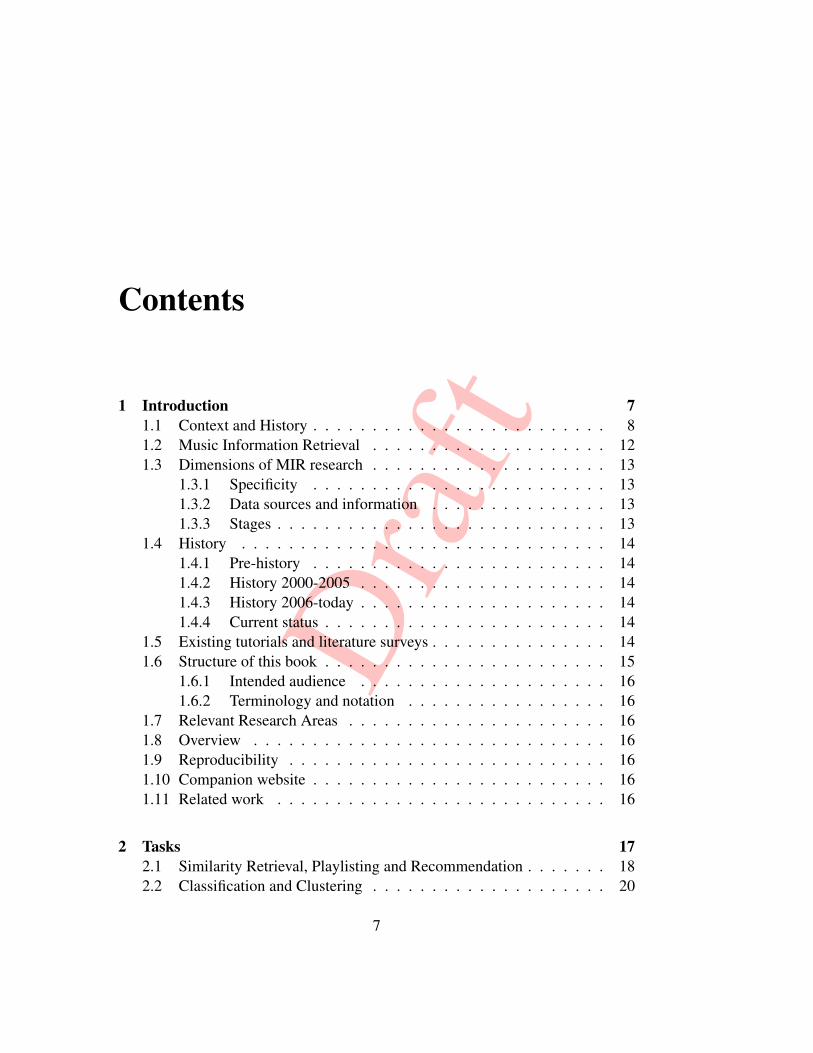
1 Introduction 71.1 Context and History . . . . . . . . . . . . . . . . . . . . . . . . . 81.2 Music Information Retrieval . . . . . . . . . . . . . . . . . . . . 121.3 Dimensions of MIR research . . . . . . . . . . . . . . . . . . . . 13
1.3.1 Specificity . . . . . . . . . . . . . . . . . . . . . . . . . 131.3.2 Data sources and information . . . . . . . . . . . . . . . 131.3.3 Stages . . . . . . . . . . . . . . . . . . . . . . . . . . . . 13
1.4 History . . . . . . . . . . . . . . . . . . . . . . . . . . . . . . . 141.4.1 Pre-history . . . . . . . . . . . . . . . . . . . . . . . . . 141.4.2 History 2000-2005 . . . . . . . . . . . . . . . . . . . . . 141.4.3 History 2006-today . . . . . . . . . . . . . . . . . . . . . 141.4.4 Current status . . . . . . . . . . . . . . . . . . . . . . . . 14
1.5 Existing tutorials and literature surveys . . . . . . . . . . . . . . . 141.6 Structure of this book . . . . . . . . . . . . . . . . . . . . . . . . 15
1.6.1 Intended audience . . . . . . . . . . . . . . . . . . . . . 161.6.2 Terminology and notation . . . . . . . . . . . . . . . . . 16
1.7 Relevant Research Areas . . . . . . . . . . . . . . . . . . . . . . 161.8 Overview . . . . . . . . . . . . . . . . . . . . . . . . . . . . . . 161.9 Reproducibility . . . . . . . . . . . . . . . . . . . . . . . . . . . 161.10 Companion website . . . . . . . . . . . . . . . . . . . . . . . . . 161.11 Related work . . . . . . . . . . . . . . . . . . . . . . . . . . . . 16
2 Tasks 172.1 Similarity Retrieval, Playlisting and Recommendation . . . . . . . 182.2 Classification and Clustering . . . . . . . . . . . . . . . . . . . . 20
7
Dra
ft
8 CONTENTS
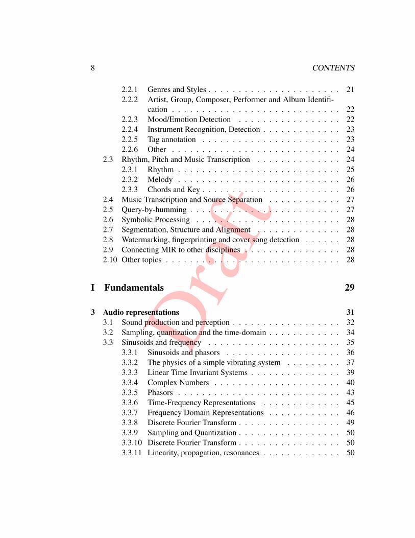
2.2.1 Genres and Styles . . . . . . . . . . . . . . . . . . . . . . 212.2.2 Artist, Group, Composer, Performer and Album Identifi-
cation . . . . . . . . . . . . . . . . . . . . . . . . . . . . 222.2.3 Mood/Emotion Detection . . . . . . . . . . . . . . . . . 222.2.4 Instrument Recognition, Detection . . . . . . . . . . . . . 232.2.5 Tag annotation . . . . . . . . . . . . . . . . . . . . . . . 232.2.6 Other . . . . . . . . . . . . . . . . . . . . . . . . . . . . 24
2.3 Rhythm, Pitch and Music Transcription . . . . . . . . . . . . . . 242.3.1 Rhythm . . . . . . . . . . . . . . . . . . . . . . . . . . . 252.3.2 Melody . . . . . . . . . . . . . . . . . . . . . . . . . . . 262.3.3 Chords and Key . . . . . . . . . . . . . . . . . . . . . . . 26
2.4 Music Transcription and Source Separation . . . . . . . . . . . . 272.5 Query-by-humming . . . . . . . . . . . . . . . . . . . . . . . . . 272.6 Symbolic Processing . . . . . . . . . . . . . . . . . . . . . . . . 282.7 Segmentation, Structure and Alignment . . . . . . . . . . . . . . 282.8 Watermarking, fingerprinting and cover song detection . . . . . . 282.9 Connecting MIR to other disciplines . . . . . . . . . . . . . . . . 282.10 Other topics . . . . . . . . . . . . . . . . . . . . . . . . . . . . . 28
I Fundamentals 29
3 Audio representations 313.1 Sound production and perception . . . . . . . . . . . . . . . . . . 323.2 Sampling, quantization and the time-domain . . . . . . . . . . . . 343.3 Sinusoids and frequency . . . . . . . . . . . . . . . . . . . . . . 35
3.3.1 Sinusoids and phasors . . . . . . . . . . . . . . . . . . . 363.3.2 The physics of a simple vibrating system . . . . . . . . . 373.3.3 Linear Time Invariant Systems . . . . . . . . . . . . . . . 393.3.4 Complex Numbers . . . . . . . . . . . . . . . . . . . . . 403.3.5 Phasors . . . . . . . . . . . . . . . . . . . . . . . . . . . 433.3.6 Time-Frequency Representations . . . . . . . . . . . . . 453.3.7 Frequency Domain Representations . . . . . . . . . . . . 463.3.8 Discrete Fourier Transform . . . . . . . . . . . . . . . . . 493.3.9 Sampling and Quantization . . . . . . . . . . . . . . . . . 503.3.10 Discrete Fourier Transform . . . . . . . . . . . . . . . . . 503.3.11 Linearity, propagation, resonances . . . . . . . . . . . . . 50
Dra
ft
CONTENTS 9
3.3.12 The Short-Time Fourier Transform . . . . . . . . . . . . . 503.3.13 Wavelets . . . . . . . . . . . . . . . . . . . . . . . . . . 51
3.4 Perception-informed Representations . . . . . . . . . . . . . . . . 513.4.1 Auditory Filterbanks . . . . . . . . . . . . . . . . . . . . 513.4.2 Perceptual Audio Compression . . . . . . . . . . . . . . . 51
3.5 Source-based Representations . . . . . . . . . . . . . . . . . . . 513.6 Further Reading . . . . . . . . . . . . . . . . . . . . . . . . . . . 51
4 Music Representations 534.0.1 Music Representations through History . . . . . . . . . . 55
4.1 Common Music Notation . . . . . . . . . . . . . . . . . . . . . . 554.2 Music Theory . . . . . . . . . . . . . . . . . . . . . . . . . . . . 554.3 Graphical Score Representations . . . . . . . . . . . . . . . . . . 554.4 MIDI . . . . . . . . . . . . . . . . . . . . . . . . . . . . . . . . 554.5 MusicXML . . . . . . . . . . . . . . . . . . . . . . . . . . . . . 55
5 Feature Extraction 575.1 Timbral Texture Features . . . . . . . . . . . . . . . . . . . . . . 58
5.1.1 Spectral Features . . . . . . . . . . . . . . . . . . . . . . 585.1.2 Mel-Frequency Cepstral Coefficients . . . . . . . . . . . 595.1.3 Other Timbral Features . . . . . . . . . . . . . . . . . . . 595.1.4 Temporal Summarization . . . . . . . . . . . . . . . . . . 615.1.5 Song-level modeling . . . . . . . . . . . . . . . . . . . . 64
5.2 Rhythm Features . . . . . . . . . . . . . . . . . . . . . . . . . . 665.2.1 Onset Strength Signal . . . . . . . . . . . . . . . . . . . 665.2.2 Tempo Induction and Beat Tracking . . . . . . . . . . . . 685.2.3 Rhythm representations . . . . . . . . . . . . . . . . . . 70
5.3 Pitch/Harmony Features . . . . . . . . . . . . . . . . . . . . . . 725.4 Other Audio Features . . . . . . . . . . . . . . . . . . . . . . . . 745.5 Bag of codewords . . . . . . . . . . . . . . . . . . . . . . . . . . 755.6 Spectral Features . . . . . . . . . . . . . . . . . . . . . . . . . . 755.7 Mel-Frequency Cepstral Coefficients . . . . . . . . . . . . . . . . 755.8 Pitch and Chroma . . . . . . . . . . . . . . . . . . . . . . . . . . 755.9 Beat, Tempo and Rhythm . . . . . . . . . . . . . . . . . . . . . . 755.10 Modeling temporal evolution and dynamics . . . . . . . . . . . . 755.11 Pattern representations . . . . . . . . . . . . . . . . . . . . . . . 755.12 Stereo and other production features . . . . . . . . . . . . . . . . 75
Dra
ft
10 CONTENTS
6 Context Feature Extraction 776.1 Extracting Context Information About Music . . . . . . . . . . . 77
7 Analysis 797.1 Feature Matrix, Train Set, Test Set . . . . . . . . . . . . . . . . . 817.2 Similarity and distance metrics . . . . . . . . . . . . . . . . . . . 817.3 Classification . . . . . . . . . . . . . . . . . . . . . . . . . . . . 81
7.3.1 Evaluation . . . . . . . . . . . . . . . . . . . . . . . . . 827.3.2 Generative Approaches . . . . . . . . . . . . . . . . . . . 837.3.3 Discriminative . . . . . . . . . . . . . . . . . . . . . . . 837.3.4 Ensembles . . . . . . . . . . . . . . . . . . . . . . . . . 837.3.5 Variants . . . . . . . . . . . . . . . . . . . . . . . . . . . 83
7.4 Clustering . . . . . . . . . . . . . . . . . . . . . . . . . . . . . . 837.5 Dimensionality Reduction . . . . . . . . . . . . . . . . . . . . . 84
7.5.1 Principal Component Analysis . . . . . . . . . . . . . . . 847.5.2 Self-Organizing Maps . . . . . . . . . . . . . . . . . . . 85
7.6 Modeling Time Evolution . . . . . . . . . . . . . . . . . . . . . . 867.6.1 Dynamic Time Warping . . . . . . . . . . . . . . . . . . 867.6.2 Hidden Markov Models . . . . . . . . . . . . . . . . . . 877.6.3 Kalman and Particle Filtering . . . . . . . . . . . . . . . 87
7.7 Further Reading . . . . . . . . . . . . . . . . . . . . . . . . . . . 87
II Tasks 89
8 Similarity Retrieval 918.0.1 Evaluation of similarity retrieval . . . . . . . . . . . . . . 95
9 Classification 999.1 Classification . . . . . . . . . . . . . . . . . . . . . . . . . . . . 999.2 Emotion/Mood . . . . . . . . . . . . . . . . . . . . . . . . . . . 1019.3 Instrument . . . . . . . . . . . . . . . . . . . . . . . . . . . . . . 1019.4 Other . . . . . . . . . . . . . . . . . . . . . . . . . . . . . . . . 1019.5 Symbolic . . . . . . . . . . . . . . . . . . . . . . . . . . . . . . 1029.6 Further Reading . . . . . . . . . . . . . . . . . . . . . . . . . . . 102
Dra
ft
CONTENTS 11
10 Structure 10310.1 Segmentation . . . . . . . . . . . . . . . . . . . . . . . . . . . . 10310.2 Alignment . . . . . . . . . . . . . . . . . . . . . . . . . . . . . . 10310.3 Structure Analysis . . . . . . . . . . . . . . . . . . . . . . . . . . 103
11 Transcription 10511.1 Monophonic Pitch Tracking . . . . . . . . . . . . . . . . . . . . 10511.2 Transcription . . . . . . . . . . . . . . . . . . . . . . . . . . . . 10511.3 Chord Detection . . . . . . . . . . . . . . . . . . . . . . . . . . . 105
12 Symbolic Representations 107
13 Queries 10913.1 Query by example . . . . . . . . . . . . . . . . . . . . . . . . . . 10913.2 Query by humming . . . . . . . . . . . . . . . . . . . . . . . . . 109
14 Fingerprinting and Cover Song Detection 11114.1 Fingerprinting . . . . . . . . . . . . . . . . . . . . . . . . . . . . 11114.2 Cover song detection . . . . . . . . . . . . . . . . . . . . . . . . 111
15 Other topics 11715.1 Optical Music Recognition . . . . . . . . . . . . . . . . . . . . . 11715.2 Digital Libraries and Metadata . . . . . . . . . . . . . . . . . . . 11715.3 Computational Musicology . . . . . . . . . . . . . . . . . . . . . 117
15.3.1 Notated Music . . . . . . . . . . . . . . . . . . . . . . . 11715.3.2 Computational Ethnomusicology . . . . . . . . . . . . . 11815.3.3 MIR in live music performance . . . . . . . . . . . . . . 118
15.4 Further Reading . . . . . . . . . . . . . . . . . . . . . . . . . . . 118
III Systems and Applications 119
16 Interaction 12116.1 Interaction . . . . . . . . . . . . . . . . . . . . . . . . . . . . . . 121
Dra
ft
12 CONTENTS
17 Evaluation 12317.1 Bibliography . . . . . . . . . . . . . . . . . . . . . . . . . . . . 123
18 User Studies 125
19 Tools 12719.1 Datasets . . . . . . . . . . . . . . . . . . . . . . . . . . . . . . . 12719.2 Digital Music Libraries . . . . . . . . . . . . . . . . . . . . . . . 129
A Statistics and Probability 131
B Project ideas 133
C Commercial activity 2011 135
D Historic Time Line 137

Dra
ftPreface
Music Information Retrieval (MIR) is a field that has been rapidly evolving since2000. It encompases a wide variety of ideas, algorithms, tools, and systems thathave been proposed to handle the increasingly large and varied amounts of musi-cal data available digitally. Researchers in this emerging field come from manydifferent backgrounds. These include Computer Science, Electrical Engineering,Library and Information Science, Music, and Psychology. They all share thecommon vision of designing algorithms and building tools that can help us orga-nize, understand and search large collections of music in digital form. However,they differ in the way they approach the problem as each discipline has its ownterminology, existing knowledge, and value system. The resulting complexity,characteristic of interdisciplinary research, is one of the main challenges facingstudents and researchers entering this new field. At the same time, it is exactlythis interdisciplinary complexity that makes MIR such a fascinating topic.
The goal of this book is to provide a comprehensive overview of past andcurrent research in Music Information Retrieval. A considerable challenge hasbeen to make the book accessible, and hopefully interesting, to readers comingfrom the wide variety of backgrounds present in MIR research. Intuition andhigh-level understanding are stressed while at the same time providing sufficienttechnical information to support implementation of the described algorithms. Thefundamental ideas and concepts that are needed in order to understand the pub-lished literature are also introduced. A thorough bibliography to the relevantliterature is provided and can be used to explore in more detail the topics coveredin this book. Throughout this book my underlying intention has been to provideenough support material to make any publication published in the proceedingsof the conference of the International Society for Music Information Retrieval(ISMIR) understandable by the readers.
1

Dra
ft
2 CONTENTS
I have been lucky to be part of the growing MIR community right from it’sinception. It is a great group of people, full of passion for their work and alwaysopen to discussing their ideas with researchers in other disciplines. If you everwant to see a musicologist explaining Shenkerian analysis to an engineer or anengineer explaining Fourier Transforms to a librarian then try attending ISMIR,the International Conference of the Society for Music Information Retrieval. Ihope this book motivates you to do so.

Dra
ftAcknowledgements
Music Information Retrieval is a research topic that I have devoted most of myadult life. My thinking about it has been influenced by many people that I havehad the fortune to interact with. As is the case in most such acknowledgementsections there are probably more names than most readers care about. At the sametime there is a good chance that I also have probably forgotten some to which Iapologize.
First of all I would like to thank my wife Tiffany and my two sons Panosand Nikos for not letting my work consume me. I am typing these sentenceson an airplane seat with my 1 year old son Nikos sleeping on my lap and my5 year old son Panos sleeping next to me. Like most kids they showed musicinformation retrieval abilities before they walked or talked. I always smile whenI remember Panos bobbing his head in perfect time with the uneven rhythms ofCretan folk music, or Nikos pointing at the iPod until the music started so thathe could swirl to his favorite reggae music. Both of these seemingly simple tasks(following a rhythm and recognizing a particular genre of music) are still beyondthe reach of computer systems today, and my sons, as well as most children theirage, can perform them effortlessly. Since 2000 me and many other researchershave explored how to computationally solve such problems utilizing techniquesfrom digital signal processing, machine and computer science. It is humbling torealize how much further we still need to go.
I would also like to thank my parents Anna and Panos who kindled my loveof music and science respectively from an early age. I also would like to thankmy uncle Andreas who introduced me to the magic of computer programmingusing Turbo Pascal (version 3) when I was a high shool student. Studying musichas always been part of my life and I owe a lot to my many music teachersover the years. I would like to single out Theodoros Kerkezos, my saxophoneteacher, who through his teaching rigor turned a self taught saxophone player
3
Dra
ft
4 CONTENTS
with many bad playing habits into a decent player with solid technique. I havealso been fortunate to play with many amazing musicians and I am constantlyamazed by what an incredible experience playing music is. I would like to thank,in somewhat chronological order: Yorgos Pervolarakis, Alexis Drakos Ktistakis,Dimitris Zaimakis, Dimitris Xatzakis, Sami Amiris, Tina Pearson and Paul Waldewith whom I have shared some of my favorite music making.
I have been very fortunate to work and learn from amazing academic mentors.As an undergraduate student, my professors Giorgos Tziritas and Apostolos Tra-ganitis at the University of Crete exposed me to research in image processingand supported my efforts to work on audio and music processing. My PhDsupervisor Perry Cook provided all the support someone could wish for, whenmy research involving computer analysis of audio representations of music sig-nals was considered a rather exotic computer science endeavor. His boundlesscreativity, enthusiasm and love of music in most (but not all) forms have alwaysbeen a source of inspiration. I am also very grateful that he never objected tome taking many music courses at Princeton and learning from amazing teachersincluding
XXX blurb about music teachers at Princeton XXXI also learned a lot from working as a postdoctoral fellow with Roger Dannen-
berg at Carnegie Mellon University. Roger was doing music information retrievallong before the term was coined. I am completely in awe of the early work he wasable to do when processing sound using computers was much more challengingthan today. When I joined Google Research as visiting faculty during a six monthsabbatical leave, I thought I had a pretty decent grasp of digital signal processing.Dick Lyon showed me how much more I needed to learn especially related tocomputer models of the human auditory system. I also learned a lot from KenSteiglitz both as a graduate student at Princeton University and later on throughhis book “A Digital Signal Processing Primer”. I consider this book the bestDSP book for beginners that I have read. It also strongly influenced the way Iapproach explaining DSP, especially for readers with no previous exposure to it inthe classes that I teach as well as this book.
Marsyas (Music Analysis, Retrieval and Synthesis for Audio Signals) is afree software framework for audio processing with specific emphasis on musicinformation retrieval that I designed and for which I am the main developer since2000. It has provided me, my students and collaborators from around the world,a set of tools and algorithms to explore music information retrieval. The coreMarsyas developers have been amazing friends and collaborators throughout theyears. I would like to particularly acknowledge, in no particular order, Ari Lazier,
Dra
ft
CONTENTS 5
Luis Gustavo Martins, Luis F. Texeira, Aaron Hechmer, Neil Burroughs, CarlosCastillio, Mathieu Lagrange, Emiru Tsunoo, Alexander Lerch, Jakob Leben andlast but by no means least, Graham Percival.
I have also been taught a lot from the large number of undergraduate andgraduate students I have worked with with over the course of my academic ca-reer. I would like to single out Ajay Kapur and Adam Tindale who through theirPhD work made me realize the potential of utilizing music information retrievaltechniques in the context of live music performance. My current PhD studentsSteven Ness and Shawn Trial helped expand the use of automatic audio analysis tobioacoustic signals and robotic music instruments respectively. Graham Percivalhas been a steady collaborator and good friend through his Masters under mysupervision, his PhD at the University of Glasgow, and 6 month post-doc workingwith me. I have also had the great fortune to work with several Postdoctoralfellows and international visiting students. Mathieu Lagrange and Luis GustavoMartins have been amazing friends and collaborators. I also had a great timeworking with and learning from Alexander Lerch, Jayme Barbedo, Tiago Tavares,Helene Papadopoulos, Dan Godlovich, Isabel Barbancho, and Lorenzo Tardon.

Dra
ft
6 CONTENTS

Dra
ftChapter 1
Introduction
I know that the twelve notes in each octave and the variety of rhythm offer meopportunities that all of human genius will never exhaust.Igor Stavinsky
In the first decade of the 21st century there has been a dramatic shift in howmusic is produced, distributed and consumed. This is a digital age where com-puters are pervasive in every aspect of our lives. Music creation, distribution,and listening have gradually become to a large extent digital. For thousandsof years music only existed while it is created at a particular time and place.Suddenly not only it can be captured through recordings but enormous amountsof it are easily accessible through electronic devices. A combination of advancesin digital storage capacity, audio compression, and increased network bandwidthhave made this possible. Portable music players, computers, and smart phoneshave facilitated the creation of personal music collections consisting of thousandsof music tracks. Millions of music tracks are accessible through streaming overthe Internet in digital music stores and personalized radio stations. It is verylikely that in the near future all of recorded music will be available and accessibledigitally.
The central challenge that research in the emerging field of music informa-tion retrieval (MIR) tries to address is how to organize and analyze these vastamounts of music and music-related information available digitally. In addition,
7

Dra
ft
8 CHAPTER 1. INTRODUCTION
it also involves the development of effective tools for listeners, musicians andmusicologists that are informed by the results of this computer supported analysisand organization. MIR is an inherently interdisciplinary field involving ideasfrom many fields including Computer Science, Electrical Engineering, Libraryand Information Science, Music, and Psychology. The field has a history ofapproximately 13 years so it is a relatively new research area. Enabling anyonewith access to a computer and the Internet to listen to essentially most of recordedmusic in human history is a remarkable technological achievement that wouldprobably be considered impossible even as recently as 15 years ago. The researcharea of Music Information Retrieval (MIR) gradually emerged during this timeperiod in order to address the challenge of effectively accessing and interactingwith these vast digital collections of music and associated information such asmeta-data, reviews, blogs, rankings, and usage/download patterns.
This book attempts to provide a comprehensive overview of MIR that is rel-atively self-contained in terms of providing the necessary interdisciplinary back-ground required to understand the majority of work in the field. The guidingprinciple when writing the book was that there should be enough backgroundmaterial in it, to support understanding any paper that has been published in themain conference of the field: the International Conf. of the Society for MusicInformation Retrieval (ISMIR). In this chapter the main concepts and ideas behindMIR as well as how the field evolved historically are introduced.
1.1 Context and History
Music is one of the most fascinating activities that we engage as a species as wellas one of the most strange and intriguing. Every culture throughout history hasbeen involved with the creation of organized collections of air pressure waves thatsomehow profoundly affect us. To produce these waves we have invented andperfected a large number of sound producing objects using a variety of materialsincluding wood, metal, guts, hair, and skin. With the assistance of these artifacts,that we call musical instruments, musicians use a variety of ways (hiting, scraping,bowing, blowing) to produce sound. Music instruments are played using everyconceivable part of our bodies and controlling them is one of the most complexand sophicated forms of interaction between a human and an artifact. For mostof us listening to music is part of our daily lives, and we find it perfectly naturalthat musicians spend large amounts of their time learning their craft, or that we

Dra
ft
1.1. CONTEXT AND HISTORY 9
frequently pay money to hear them perform. Somehow these organized structuresof air pressure waves are important enough to warrant our time and resources andas far as we can tell this has been a recurring pattern throughout human historyand different cultures. It is rather perplexing how much time and energy we arewilling to put into music making and listening and there is vigorous debate aboutwhat makes music so important. What is clear is that music was, is, and probablywill be an essential part of our lives.
Technology has always played a vital role in music creation, distribution, andlistening. Throughout history the making of musical instruments has followedthe technological trends of the day. For example instrument making has takenadvantage of progressively better tools for wood and bone carving, the discoveryof new metal alloys, and materials imported from far away places. In addition,more conceptual technological developments such as the use of music notationto preserve and transmit music, or the invention of recording technology havealso had profound implications on how music has been created and distributed.In this section, a brief overview of the history of how music and music-relatedinformation has been transmitted and preserved across time and space is provided.
Unlike painting or sculpture, music is emphemeral and exists only during thecourse of a performance and as a memory in the minds of the listeners. It isimportant to remember that this has been the case throughout most of humanhistory. Only very recently with the invention of recording technology couldmusic be “preserved” across time and space. The modern term “live” musicapplied to all music before recording was invented. Music is a process not anartifact. This fleeting nature made music transmission across space and timemuch more difficult than other arts. For example, although we know a lot aboutwhat instruments and to some extent what music scales were used in antiquity,we have very vague ideas of how the music actually sounded. In contrast, wecan experience ancient sculptures or paintings in a very similar way to how theywere perceived when they were created. For most of human history the onlymeans of transmission and preservation of musical information was direct contactbetween a performer and a listener during a live performance. The first majortechnological development that changed this state of affairs was the inventionof musical notation. Although several forms of music notation exist for ourdiscussion we will focus on the evolution of Western common music notationwhich today is the most widely used music notation around the world.
Several music cultures around the world developed symbolic notation systemsalthough musicians today are mostly familiar with Western common music no-tation. The origins of western music notation lie in the use of written symbols
Dra
ft
10 CHAPTER 1. INTRODUCTION
as mnemonic aids in assisting singers render melodically a particular religioustext. Fundamentally the basic idea behind music notation systems is to encodesymbolically information about how a particular piece of music can be performed.In the same way that a recipe is a set of instructions for making a particular dish, anotated piece of music is a set of instructions that musicians must follow to rendera particular piece of music. Gradually music notation became more precise andable to capture more information about what is being performed. However it canonly capture some aspects of a music performance which leads to considerablediversity in how musicians interpret a particular notated piece of music. Thelimitated nature of music notation is because of its discrete symbolic nature andthe limited amount of possible symbols one can place on a piece of paper and real-istically read. Although initially simply a mnemonic aid, music notation evolvedand was used as a way to preserve and transmit musical information across spaceand time. Music notation provided an alternative way of encountering new musicto attending a live performance. For example, a composer like J. S. Bach couldhear music composed in Italy by simply reading a piece of paper and playing iton a keyboard rather than having to physically be present when it was performed.Thanks to written music scores any keyboard player today can still perform thepieces J. S. Bach composed more than 300 hundred years ago by simply readingthe scores he wrote. One interesting sidenote that is a recurring theme in thehistory of technology and music technology is that frequently inventions are usedin ways that their original creators never envisioned. Although originally con-ceived more as a mnemonic aid for existing music, music notation profoundly hasaffected the way music was created, distributed and consumed. For example, theadvent of music notation to a large extent was the catalyst that enabled the creationof a new type of specialized worker the freelance composer who supported himselfby selling his scores rather than requiring a rich patron to support him.
The invention of recording technology caused even more significant changesin the way music was created, distributed and consumed. The history of recordingand the effects it had is extremely fascinating. In many ways it is also quiteinformative about many of the debates and discussions about the role of digitalmusic technology today. Recording enabled repeatability at a much more preciselevel than music notation ever could and decouples the process of listening fromthe process of music making.
Given the enormous impact of recording technology to music it is hard toimagine that there was a time when it was considered a distraction from the “real”application of recording speech for business applications by none less than thedistinguished Thomas Edison. Despite his attempts music recordings became

Dra
ft
1.1. CONTEXT AND HISTORY 11
extremely popular and jukebox sales exploded. For the first time in history musiccould be captured, replicated and distributed across time and space and recordingdevices quickly spread across the world. The ensuing cross-polination of diversemusical styles triggered the generation of various music styles that essentiallyform the foundation of many of the popular music genres today.
Initially the intention of recordings was to capture as accurately as possiblethe sound of live music performances. At the same time, limitations of earlyrecording technology such as the difficulty of capturing dynamics and the shortduration of recordings forced musicians to modify and adapt how they playedmusic. As technology progressed with the development of inventions such aselectric microphones and magnetic tapes, recordings progressively became moreand more a different art form. Using effects such as overdubbing, splicing, andreverb recordings in many cases became creations impossible to recreate in livemusic performance.
Early gramophones allowed their owners to make their own recordings butsoon after with the standarization and mass production of recording discs theplayback devices were limited to playing not recording. Recordings becamesomething to be collected, prized and owned. They also created a different wayof listening that could be conducted in isolation. It is hard for us to imagine howstrange this isolated listening to music seemed in the early days of recording.
These two historical developments in music technology: musical notationand audio recording, are particularly relevant to the field of MIR, which is thefocus of this book. They are directly reflected in the two major types of digitalrepresentations that have been used for MIR: symbolic and audio-based. Thesedigital representations were originally engineered to simply store digitally thecorresponding analog (for example vinyl) and physical (for example typeset pa-per) information but eventually were utilized to develop completely new ways ofinteracting with music using computers. It is also fascinating how the old debatescontrasting the individual model of purchasing recordings with the broadcastingmodel of radio are being replayed in the digital domain with digital music storesthat sell individual tracks and subscription services that provided unlimited accessto streaming tracks.
Dra
ft
12 CHAPTER 1. INTRODUCTION
1.2 Music Information Retrieval
As we discussed in the previous section the ideas behind music information andretrieval are not new although the term itself is. In this book we focus on themodern use of the term music information retrieval which will be abbreviated toMIR for the remainder of the book. MIR deals with the analysis and retrieval ofmusic in digital form. It reflects the tremendous recent growth of music-relateddata digitally available and the consequent need to search within it to retrievemusic and musical information efficiently and effectively.
Arguably the birth of Music Information Retrieval (MIR) as a separate re-search area happened in Plymouth, Massachusetss in 1999 at the first conference(then symposium) on Music Information Retrieval. Although work in MIR hadappeared before that time in various venues, it wasn’t identified as such and theresults were scattered in different communities and publication venues. Duringthat Symposium a group of Computer Scientists, Electrical Engineers, Informa-tion Scientists, Musicologists, and Librarians met for the first time in a commonspace, exchanged ideas and found out what types of MIR research were happeningat the time that until then were published in completely separate and differentconferences and communities.
When MIR practitioners convey what is Music Information Retrieval to a moregeneral audience they frequently use two metaphors that capture succintly how themajority, but not all, of MIR research could potentially be used. The first metaphoris the so called “grand celestial jukebox in the sky” and refers to the potentialavailability of all recorded music to any computer user. The goal of MIR researchis to develop better ways of browsing, choosing, listening and interacting withthis vast universe of music and associated information. To a large extent onlinemusic stores, such as the iTunes store, are well on their way of providing accessto large collections of music from around the world. A complimentary metaphorcould be termed the “absolute personalized radio” in which the listening habitsand preferences of a particular user are analyzed and/or specified and computeralgorithms provide a personalized sequence of music pieces that is customized tothe particular user. As is the case with the traditional jukebox and radio for thefirst the emphasis is on choice by the user versus choice by some expert entity forthe second. It is important to note that there is also MIR research that does notfit well in these two metaphors. Examples include: work on symbolic melodicpattern segmentation or work on computational ethnomusicology.

Dra
ft
1.3. DIMENSIONS OF MIR RESEARCH 13
1.3 Dimensions of MIR researchThere are multiple different ways that MIR research can be organized into the-matic areas. Three particular “dimensions” of organization, that I have founduseful when teaching and thinking about the topic are: 1) specificity which refersto the semantic focus of the task, and 2) data sources which refers to the variousrepresentations (symbolic, meta-data, context, lyrics) 30 utilized to achieve aparticular task and 3) stages which refers to the common processing stages ina MIR systems such as representation, analysis, and interaction. In the next threesubsections, these dimensions are described in more detail.
1.3.1 Specificity
1.3.2 Data sources and information
1.3.3 Stages• Representation - Hearing
Audio signals are stored (in their basic uncompressed form) as a time seriesof numbers corresponding to the amplitude of the signal over time. Al-though this representation is adequate for transmission and reproduction ofarbitrary waveforms, it is not particularly useful for analyzing and under-standing audio signals. The way we perceive and understand audio signalsas humans is based on and constrained by our auditory system. It is wellknown that the early stages of the human auditory system (HAS) decomposeincoming sound waves into different frequency bands to a first approxima-tion. In a similar fashion, in MIR, time-frequency analysis techniques arefrequently used for representing audio signals. The representation stage ofthe MIR pipeline refers to any algorithms and systems that take as inputsimple time-domain audio signals and create a more compact, information-bearing representations. The most relevant academic research area to thisstage is Digital Signal Processing (DSP).
• Analysis - UnderstandingOnce a good representation is extracted from the audio signal various typesof automatic analysis can be performed. These include similarity retrieval,

Dra
ft
14 CHAPTER 1. INTRODUCTION
classification, clustering, segmentation, and thumbnailing. These higher-level types of analysis typically involve aspects of memory and learningboth for humans and machines. Therefore Machine Learning algorithmsand techniques are important for this stage.
• Interaction - Acting
When the signal is represented and analyzed by the system, the user mustbe presented with the necessary information and act according to it. Thealgorithms and systems of this stage are influence by ideas from HumanComputer Interaction and deal with how information about audio signalsand collections can be presented to the user and what types of controls forhandling this information are provided.
1.4 HistoryIn this section, the history of MIR as a field is traced chronologically mostlythrough certain milestones.
1.4.1 Pre-history
1.4.2 History 2000-2005The first activities in MIR were initated through activities in the digital librariescommunity [5].
1.4.3 History 2006-today
1.4.4 Current status
1.5 Existing tutorials and literature surveysOverviews

Dra
ft
1.6. STRUCTURE OF THIS BOOK 15
1.6 Structure of this book
Even though MIR is a relatiely young research area, the variety of topics, disci-plines and concepts that have been explored make it a hard topic to cover compre-hensively. It also makes a linear exposition harder. One of the issues I struggledwith while writing this book was whether to narrow the focus to topics that I wasmore familiar (for example only covering MIR for audio signals) or attempt toprovide a more complete coverage and inevitably write about topics such as sym-bolic MIR and optical music recognition (OMR) with which I was less familiar.At the end I decided to attempt to cover all topics as I think they are all importantand wanted the book to reflect the diversity of research in this field. I did mybest to familiarize myself with the published literature in topics removed from myexpertise and received generous advice and help from friends who are familiarwith them to help me write the corresponding chapters.
The organization and chapter structure of the book was another issue I strug-gled with. Organizing a particular body of knowledge is always difficult and this ismade even more so in an interdisciplinary field like MIR. An obvious organizationwould be historical with different topics introduced chronologically based on theorder they appeared in the published literature. Another alternative would bebased an organization based on MIR tasks and applications. However, there areseveral concepts and algorithms that are fundamental to and shared by most MIRapplications. After several attempts I arrived at the following organization whichalthough not perfect was the best I could do. The book is divided into three largeparts. The first, titled Fundamentals, introduces the main concepts and algorithmsthat have been utilized to perform various MIR tasks. It can be viewed as a crashcourse in important fundamental topics such as digital signal processing, machinelearning and music theory through the lens of MIR research. Readers with moreexperience in a particular topic can easily skip the corresponding chapter andmove to the next part of the book. The second part of the book, titled Tasks,describes various MIR tasks that have been proposed in the literature based on thebackground knowledge described in the Fundamentals part. The third part, titledSystems and Applications, provides a more implementation oriented exposition ofmore complete MIR systems that combine MIR tasks as well as information abouttools and data sets. Appendices provide supplementary background material aswell as some more specific optional topics.

Dra
ft
16 CHAPTER 1. INTRODUCTION
1.6.1 Intended audience
1.6.2 Terminology and notationinformatics, retrieval
piece, track, songdatabase, collection, librarymodern popular music, western art musicMIDImonophonic polyphonicsymbolic vs audiox(t) vs x[t] lower case of time domain and upper case for frequency domain
1.7 Relevant Research Areas
1.8 Overview
1.9 Reproducibility
1.10 Companion website
1.11 Related work

Dra
ftChapter 2
Tasks
Like any researh area, Music Information Retrieval (MIR) is characterized by thetypes of problems researchers are working on. In the process of growing as afield, more and hopefully better algorithms for solving each task are constantydesigned, described and evaluated in the literature. In addition occassionallynew tasks are proposed. The majority of these tasks can easily be describedto anyone with a basic understanding of music. Moreover they are tasks thatmost humans perform effortlessly. A three year old child can easily peformmusic information related tasks such as recognizing a song, clapping along withmusic, or listening to the sung words in a complex mixture of instrumental soundsand voice signals. At the same time, the techniques used to perform such tasksautomatically are far from simple. It is humbling to realize that a full arsenalof sophisticated signal processing and machine learning algorithms are requiredto perform these seemingly simple music information tasks using computers. Atthe same time computers, unlike humans, can process arbitrarily large amounts ofdata and that way open up new possibilities in how listeners interact with largedigital collections of music and associated information. For example, a computercan analyze a digital music collection with thousands of songs to find pieces ofmusic that share a particular melody or retrieve several music tracks that matchan automatically calculated tempo. These are tasks beyond the ability of mosthumans when applied to large music collections. Ultimately MIR research shouldbe all about combining the unique capabilities of humans and machines in thecontext of music information and interaction.
17
Dra
ft
18 CHAPTER 2. TASKS
In this chapter, a brief overview of the main MIR tasks that have been proposedin the literature and covered in this book is provided. The goal is to describehow each task/topic is formulated in terms of what it tries to achieve rather thanexplaining how these tasks are solved or how algorithms for solving them areevaluated. Moreover, the types of input and output required for each task arediscussed. In most tasks there is typically a seminal paper or papers that had alot of impact in terms of formulating the task and influencing subsequent work.In many cases these seminal papers are preceded by earlier attempts that did notgain traction. For each task described in this chapter I attempt, to the best of myknowledge, to provide pointers to the earliest relevant publication, the seminalpublication and some representative examples. Additional citations are providedin the individual chapters in the rest of the book.
This chapter can also be viewed as an attempt to organize the growing andsomewhat scattered literature in MIR into meaningful categories and serve as aquick reference guide. The rest of the book is devoted to explaining how we candesign algorithms and build systems to solve these tasks. Solving these tasks cansometimes directly result in useful systems, but frequently they form componentsof larger more complicated and complex systems. For example beat tracking canbe considered a MIR task, but it can also be part of a larger computer-assisted DJsystem that performs similarity retrieval and beat alignment. Monophonic pitchextraction is another task that can be part of a larger query-by-humming system.Roughly speaking I consider as a task any type of MIR problem for which there isexisting published work and there is a clear definition of what the expected inputand desired output should be. The order of presentation of tasks in this chapter isrelatively subjective and the descriptions are roughly proportional to the amountof published literature in each particular task.
2.1 Similarity Retrieval, Playlisting and Recommen-
dationSimilarity retrieval (or query-by-example) is one of the most fundamental MIRtasks. It is also one of the first tasks that were explored in the literature. Itwas originally inspired by ideas from text information retrieval and this earlyinfluence is reflected in the naming of the field. Today most peope with computersuse search engines on a daily basis and are familiar with the basic idea of text
Dra
ft
2.1. SIMILARITY RETRIEVAL, PLAYLISTING AND RECOMMENDATION19
information retrieval. The user submits a query consisting of some words to thesearch engine and the search engine returns a ranked list of web pages sorted byhow relevant they are to the query.
Similarity retrieval can be viewed as an analogous process where instead of theuser querying the system by providing text the query consists of an actual pieceof music. The system then responds by returning a list of music pieces ranked bytheir similarity to the query. Typically the input to the system consists of the querymusic piece (using either a symbolic or audio representation) as well as additionalmetadata information such as the name of the song, artist, year of release etc. Eachreturned item typically also contains the same types of meta-data. In addition tothe audio content and meta-data other types of user generated information can alsobe considered such as ranking, purchase history, social relations and tags.
Similarity retrieval can also be viewed as a basic form of playlist generation inwhich the returned results form a playlist that is “seeded” by the query. Howevermore complex scenarios of playlist generation can be envisioned. For example astart and end seed might be specified or additional constraints such as approximateduration or minimum tempo variation can be specified. Another variation is basedon what collection/database is used for retrieval. The term playlisting is morecommonly used to describe the scenario where the returned results come from thepersonal collection of the user, while the term recommendation is more commonlyused in the case where the returned results are from a store containing a largeuniverse of music. The purpose of the recommnedation process is to entice theuser to purchase more music pieces and expand their collection. Although thesethree terms (similarity retrieval, music recommendation, automatic playlisting)have somewhat different connotations the underlying methodology for solvingthem is similar so for the most part we will use them interchangeably. Anotherrelated term that is sometimes used in personalized radio in which the idea is toplay music that is personalized to the preferences to the user.
One can distinguish three basic approaches to computing music similarity.Content-based similarity is performed by analyzing the actual content to extractthe necessary information. Metadata approaches exploit sources of informationthat are external to the actual content such as relationships between artists, styles,tags or even richer sources of information such as web reviews and lyrics. Usage-based approaches track how users listen and purchase music and utilize this infor-mation for calculating similarity. Examples include collaborive filtering in whichthe commonalities between purchasing histories of different users are exploited,tracking peer-to-peer downloads or radio play of music pieces to evaluate their“hotness” and utilizing user generated rankings and tags.

Dra
ft
20 CHAPTER 2. TASKS
There are trade-offs involved in all these three approaches and most likelythe ideal system would be one that combines all of them intelligently. Usage-based approaches suffer from what has been termed the “cold-start” problem inwhich new music pieces for which there is no usage information can not be rec-ommended. Metadata approaches suffer from the fact that metadata information isfrequently noisy or inaccurate and can sometimes require significant semi-manualeffort to clean up. Finally content-based methods are not yet mature enough toextract high-level information about the music.
Evaluation of similarity retrieval is difficult as it is a subjective topic andtherefore require large scale user studies in order to be properly evaluated. In mostpublished cases similarity retrieval systems are evaluated through some relatedtasks such how many of the returned music tracks belong to the same genre as thequery.
2.2 Classification and Clustering
Classification refers to the process of assigning one or more textual labels inorder to characterize a piece of music. Humans have an innate drive to groupand categorize things including music pieces. In classification tasks the goal isgiven a piece of music to perform this grouping and categorization automatically.Typically this is achieved by automatically analyzing a collection of music thathas been manually annotated with the corresponding classification information.The analysis results are used to “train” models (computer algorithms) that giventhe analysis results (referred to as audio features) for a new unlabelled musictrack are able “predict” the classification label with reasonable accuracy. This isreferred to as “supervised learning” in the field of machine learning/data mining.At the opposite end of the spectrum is “unsupervised learning” or “clustering” inwhich the objects of interest (music pieces in our case) are automatically groupedtogether into “clusters” such that pieces that are similar fall in the same cluster.
There are several interesting variants and extensions of the classic problemsof the classification and clustering. In semi-supervised learning the learning algo-rithms utilizes both labeled data as in standard classification as well as unlabeleddata as in clustering. The canonical output of classification algorithms is a singlelabel from a finite known set of classification lables. In multi-label classificationeach object to be classified is associated with multiple labels both when trainingand predicting.

Dra
ft
2.2. CLASSIFICATION AND CLUSTERING 21
When characterizing music several possible such groupings have been usedhistorically as means of organizing music and computer algorithms that attempt toperform the categorization automatically have been developed. Although the mostcommon input to MIR classification and clustering systems is audio signals therehas also been work that utilizes symbolic representations as well as metadata (suchas tags and lyrics) and context information (peer-to-peer downloads, purchasehistory). In the following subsections, several MIR tasks related to classificationand clustering are described.
2.2.1 Genres and Styles
Genres or styles are words used to describe groupings of musical pieces that sharesome characteristics. In the majority of cases these characteristics are relatedto the musical content but not always (for example in Christian Rap). Theyare used to physically organize content in record stores and virtually organizemusic in digital stores. In addition they can be used to convey music preferencesand taste as the stereotypical response to the question “What music you like”which typically goes something like “I like all different kinds of music exceptX” where X can be classical, country, heavy metal or whatever other genre theparticular person is not fond of. Even though there is clear shared meaning amongdifferent individual when discussing genres their exact definitation and boundariesare fuzzy and subjective. Even though sometimes they are criticized as beingdriven by the music industry their formation can be an informal and fascinatingprocess 1.
Top level genres like “classical” or “rock” tend to encompass a wide varietyof music pieces with the extreme case of “world music” which has enormousdiversity and almost no discriptive capability. On the other hand, more specializedgenres (sometimes refered to as sub-genres) such Neurofunk or Speed Metal aremeaningful to smaller groups of people and in many cases used to differentiate theinsiders from the outsiders. Automatic genre classification was one of the earliestclassification problems tackled in the music information retrieval literature and isstill going strong. The easy availability of ground truth (especially for top-levelgenres) that can be used for evaluation, and the direct mapping of this task to wellestablished supervised machine learning techniques are the two main reasons for
1http://www.guardian.co.uk/music/2011/aug/25/
origins-of-music-genres-hip-hop (accessed September 2011)

Dra
ft
22 CHAPTER 2. TASKS
the popularity of automatic genre classification. Genre classification can be casteither as the more common single-label classification problem (in which one out ofa set of N genres is selected for unknown tracks) or as a multi-label classificationin which a track can belong to more than one category/genre.
[64]
2.2.2 Artist, Group, Composer, Performer and Album Identi-
fication
Another obvious grouping that can be used for classification is identifying theartist or group that performs a particular music track. In the case of rock andpopular music frequently the performing artists are also the composers and thetracks are typically associated to a group (like the Beatles or Led Zeppelin). Onthe other hand in classical music there is typically a clearer distinction betweencomposer and performer. The advantage of artist identification compared to genreis that the task is much more narrow and in some ways well-defined. At thesame time it has been criticized as identifying the production/recording approachused, rather than the actual musical content (especially in the case of songs fromthe same album) and also being a somewhat artifical tasks as in most practicalscenarios this information is readily available from meta-data.
2.2.3 Mood/Emotion Detection
Music can evoke a wide variety of emotional responses which is one of the reasonsit is heavily utilized during movies. Even though culture and education can sig-nificantly affect the emotional response of listeners to music there has been workattempting to automatically detection mood and emotion in music. As this is in-formation that listeners frequently used to discuss music and not readily availablein most cases there has been considerable interest in performing it automatically.Even though it is occassionally cast as a single-label classification problem it ismore appropriately considered a multi-label problem or in some cases a regressionin a continuous “emotion” space.
Dra
ft
2.2. CLASSIFICATION AND CLUSTERING 23
2.2.4 Instrument Recognition, Detection
Monophonic instrument recognition refers to automatically predicting the name/typeof a recorded sample of a musical instrument. In the easiest configuration isolatednotes of the particular instrument are provided. A more complex scenario is whenlarger phrases are used, and of course the most difficult problem is identifyingthe instruments present in a mixture of musical sounds (polyphonic instrumentrecognition or instrumentation detection). Instrument classification techniquesare typically applied to databases of recorded samples.
2.2.5 Tag annotation
The term “tag” refers to any keyword associated to an article, image, video, orpiece of music on the web. In the past few years there has been a gradual shiftfrom manual annotation into fixed hierarchical taxonomies to collaborative socialtagging where any user can annotate multimedia objects with tags (so called folk-sonomies) without conforming to a fixed hierarchy and vocabulary. For example,Last.fm is a collaborative social tagging network which collects roughly 2 milliontags (such as “saxophone”, “mellow”, “jazz”, “happy”) per month [?] and usesthat information to recommend music to its users. Another source of tags are“games with a purpose” [?] where people contribute tags as a by-product of doinga task that they are naturally motivated to perform, such as playing casual webgames. For example TagATune [?] is a game in which two players are asked todescribe a given music clip to each other using tags, and then guess whether themusic clips given to them are the same or different.
Tags can help organize, browse, and retrieve items within large multimediacollections. As evidenced by social sharing websites including Flickr, Picasa,Last.fm, and You Tube, tags are an important component of what has been termedas “Web 2.0”. The focus of MIR research is systems that automatically predicttags (sometimes called autotags) by analyzing multimedia content without re-quiring any user annotation. Such systems typically utilize signal processing andsupervised machine learning techniques to “train” autotaggers based on analyzinga corpus of manually tagged multimedia objects.
There has been considerable interest for automatic tag annotation in multi-media research. Automatic tags can help provide information about items thathave not been tagged yet or are poorly tagged. This avoids the so called “cold-start problem” [?] in which an item can not be retrieved until it has been tagged.

Dra
ft
24 CHAPTER 2. TASKS
Addressing this problem is particularly important for the discovery of new itemssuch as recently released music pieces in a social music recommendation system.
2.2.6 Other
Audio classification techniques have also been applied to a variety of other areasin music information retrieval and more generally audio signal processing. Forexample they can be used to detect which parts of a song contain vocals (singingidentification) or detect the gender of a singer. They can also be applied to theclassification/tagging of sound effects for movies and games (such as door knocks,gun shots, etc). Another class of audio signals to which similar analysis andclassification techniques can applied are bioacoustic signals which are the soundsanimals use for communication. There is also work on applying classificationtechniques on symbolic representations of music.
2.3 Rhythm, Pitch and Music TranscriptionMusic is perceived and represented at multiple levels of abstraction. At the oneextreme, an audio recording appears to capture every detailed nuance of musicperformance for prosperity. However, even in this case this is an illusion. Manydetails of a performance are lost such as the visual aspects of the performers andmusician communication or the intricacies of the spatial reflections of the sound.At the same time, a recording does capture more concrete, precise informationthan any other representation. At the other extreme a global genre categorizationof a music piece such as saying this is a piece of reggae or classical music reducesa large group of different pieces of music that share similar characteristics to a sin-gle world. In between these two extremes there is a large number of intermediatelevels of abstraction that can be used to represent the underlying musical content.
One way of thinking about these abstractions are as different representationsthat are invariant to transformations of the underlying music. For example mostlisteners, with or without formal musical training, can recognize the melody ofTwinkle, Twinkle Little Star (or some melody they are familiar with) indepen-dently of the instrument it is played on, or how fast it is played, or what is thestarting pitch. Somehow the mental representation of the melody is not affectedby these rather drastic changes to the underlying audio signal. In music theory a
Dra
ft
2.3. RHYTHM, PITCH AND MUSIC TRANSCRIPTION 25
common way of describing music is based on rhythm and pitch information. Fur-thermore, pitch information can be abstracted as melody and harmony. A westerncommon music score is a comprehensive set of notation conventions that representwhat pitches should be played, when they should be played and for how long,when a particular piece of music is performed. In the following subsections wedescribe some of the MIR tasks that can be formulated as automatically extractinga variety representations at the different levels of musical abstraction.
2.3.1 RhythmRhythm refers to the hierarchical repetitive structure of music over time. Althouhnot all music is structured rhythmically, a lot of music in the world is and haspatterns of sounds that repeat periodically. These repeating patterns are typicallyformed on top of a underlying conceptual sequence of semi-regular pulses that aregrouped hierarchically.
Automatic rhythm analysis tasks attempt to extract different kinds of rhythmicinformation from audio signals. Although there is some variability in terminoloythere are certain tasks that are sufficiently well-defined and for which severalalgorithms have been proposed.
Tempo induction refers to the process of extracting an estimate of the tempo(the frequency of the main metrical level i.e the frequency that most humans wouldtap their foot when listening to the music) for a track or excerpt. Tempo inductionis mostly meaningful for popular music with a relatively steady beat that staysthe same throughout the audio that is analyzed. Beat tracking refers to the moreinvolved process of identifying the time locations of the individual beats and isstill applicable when there are significant tempo changes over the course of thetrack being analyzed.
In addition to the two basic tasks of tempo induction and beat tracking thereare additional rhythm-related tasks that have been investigated to a smaller extent.Meter estimation refers to the process of automatically detecting the groupingof beat locations into large units called measures such as 4/4 (four beats permeasure) or 3/4 (3 beats per measure). A related task is the automatic extractionof rhythmic patterns (repeating sequences of drum sounds) typically found inmodern popular music with drums. Finally drum transcription deals with theextraction of a “score” notating which drum sounds are played and when in pieceof music. Early work focused on music containing only percussion [?] but morerecent work considers arbitrary polyphonic music. There is also a long history
Dra
ft
26 CHAPTER 2. TASKS
of rhythmic analysis work related to these tasks performed on symbolic repre-sentations (mostly MIDI) in many cases predating the birth of MIR as a researchfield.
2.3.2 MelodyMelody is another aspect of music that is abstract and invariant to many transfor-mations. Several tasks related to melody have been proposed in MIR. The resultof monophonic pitch extraction is a time-varying estimate of the fundamental fre-quency of a musical instrument or human voice. The output is frequently referredto as a pitch contour. Monophonic pitch transcription refers to the process ofconverting the continuous-valued pitch contour to discrete notes with a specifiedstart and duration. Figure ?? shows visually these concepts. When the music ispolyphonic (more than one sound source/music instrument is present) then the re-lated problem is termed predominant melody extraction. In many styles of musicand especially modern pop and rock there is a clear leading melodic line typicallyperformed by a singer. Electric guitars, saxophones, trumpets also frequentlyperform leading melodic lines in polyphonic music. Similalry to monophonicmelody extraction in some cases a continuous fundamental frequency contour isextracted and in other cases a discrete set of notes with associated onsets andoffests is extracted.
A very imprortant and not at all straightforward task is melodic similarity.Once these melodic representations are computed it investigates how they can becompared with each other so that melodies that would be perceived by humansas associated with the same piece of music or as similar will be automaticallydetected as such. The reason this task is not so simple is that there is an enormousamount of variations that can be applied to a melody while it still maintainsits identity. These variations range from the straightforward transformations ofpitch transposition and changing tempo to complicated aspects such as rhythmicelaboration and the introduction of new pitches.
Make figure
of melodic
variations
Make figure
of melodic
variations
[8]
2.3.3 Chords and KeyChord Detection, Key Detection/tonality
Dra
ft
2.4. MUSIC TRANSCRIPTION AND SOURCE SEPARATION 27
2.4 Music Transcription and Source Separation
Ultimately music is an organized collection of individual sound sources. Thereare several MIR tasks that can be performed by characterizing globally and statis-tically the music signal without individually characterizing each individual soundsource. At the same time it is clear that as listeners we are able to focus onindividual sound sources and extract information from them. In this section wereview different approaches to extracting information for individual sound sourcesthat have been explored in the literature.
Source separation refers to the process of taking as input a polyphonic mixtureof individual sound sources and producing as output the individual audio signalscorresponding to each individual sound source. The techniques used in this taskhave their origins in speech separation research which frequently is performedusing multiple microphones for input. Blind sound separation refers ... .
blind source separation, computational auditory scene analysis, music under-standing
2.5 Query-by-humming
In query by humming (QBH) the input to the system is a recording of a usersinging or humming the melody of a song. The output is an audio recordingthat corresponds to the hummed melody selected from a large datatabse of songs.Earlier systems constrained the user input, for example by requiring the user tosing usign fixed syllables such as La, La, La or even just the rhythm (query bytapping) with the maching being against small music collections. Current systemshave removed these restrictions accepting as input normal singing and performingthe matching against larger music collections. QBH is particularly suited for smartphones. Some related tasks that have also been explored are query by beat boxingin which the input is a vocal rendering of a particular rhythmic pattern and theoutput is either a song or a drum loop that corresponds to the vocal rhythmicpattern.
[?]
Dra
ft
28 CHAPTER 2. TASKS
2.6 Symbolic Processingrepresentations [37]
searching for motifs/themes, polyphonic search
2.7 Segmentation, Structure and Alignment[?] [32]
thumbnailing, summaring
2.8 Watermarking, fingerprinting and cover song de-
tection
2.9 Connecting MIR to other disciplinesThe most common hypothetical scenario for MIR systems is the organization andanalysis of large music collections of either popular or classical music for theaverage listener. In addition there has been work in connecting MIR to otherdisciplines such as digital libraries [5, 26], musicology [13].
2.10 Other topicsComputational musicology and ethnomusicology, performance analysis such asextracting vibrato from monophonic instruments [9], optical music recognition[?], digital libraries, standards (musicXML), assistive technologies [36], symbolicmusicology, hit song science

Dra
ftPart I
Fundamentals
29

Dra
ft
Dra
ftChapter 3
Audio representations
Is it not strange that sheep’s guts should hale souls out of men’s bodiesShakespeare
The most basic and faithful way to preserve and reproduce a specfic musicperformance is as an audio recording. Audio recordings in analog media suchas vinyl or magnetic tape degrade over time eventually becoming unusable. Theability to digitize sound means that extremely accurate reproductions of soundand music can be retained without any loss of information stored as patternsof bits. Such digital representations can theoretically be transferred indefinitelyacross different physical media without any loss of information. It is a remarkabletechnological achievement that all sounds that we can hear can be stored as anextremely long string of ones and zeroes. The automatic analysis of music storedas a digital audio signal requires a sophisticated process of distilling informationfrom an extremely large amount of data. For example a three minute song storedas uncompressed digital audio is represented digitally by a sequence almost of16 million numbers (3 (minutes) * 60 (seconds) * 2 (stereo channels) * 44100(sampling rate)) or 16 * 16 million = 256 million bits. As an example of extremedistilling of information in the MIR task of tempo induction these 16 millionnumbers need to somehow be converted to a single numerical estimate of thetempo of the piece.
In this chapter we describe how music and audio signals in general can berepresented digitally for storage and reproduction as well as describe audio repre-sentations that can be used as the basis for extracting interesting information from
31

Dra
ft
32 CHAPTER 3. AUDIO REPRESENTATIONS
these signals. We begin by describing the process of sound generation and ouramazing ability to extract all sorts of interesting information from what we hear.In order for a computer to analyze sound, it must be represented digitally. Themost basic digital audio representation is a sequence of quantized pulses in timecorresponding to the discretized displacement of air pressure that occured whenthe music was recorded. Humans (and many other organisms) make sense of theirauditory environment by identifying periodic sounds with specific frequencies. Ata very fundamental level music consists of sounds (some of which are periodic)that start and stop at different moments in time. Therefore representations ofsound that have a separate notion of time and frequency are commonly used asthe first step in audio feature extraction and are the main topic of this chapter. Westart by introducing the basic idea of a time-frequency representation. The basicconcepts of sampling and quantization that are required for storing sound digitallyare then introduced. This is followed by a discussion of sinusoidal signals whichare in many ways fundamental to understanding how to model sound mathemat-ically. The discrete Fourier transform (DFT) is one of the most fundamental andwidely used tools in music information retrieval and more generally digital signalprocessing. Therefore, its description and interpretation forms a large part of thischapter. Some of the limitations of the DFT are then discussed in order to motivatethe description of other audio representations such as wavelets and perceptuallyinformed filterbanks that conclude this chapter.
3.1 Sound production and perception
Sound and therefore music are created by moving objects whose motion resultsin changes in the surrounding air pressure. The changes in air pressure propa-gate through space and if they reach a flexible object like our eardrums or themembrane of a microphone they cause that flexible object to move in a similarway that the original sound source did. This movement happens after a short timedelay due to the time it takes for the “signal” to propagate through the medium(typically air). Therefore we can think of sound as either time-varying air-pressurewaves or time-varying displacement of some membrane like the surface of a drumor the diaphragm of a microphone. Audio recordings capture and preserve thistime-varying displament information and enable reproduction of the sound byrecreating a similar time-varying displament pattern by means of a loudspeakerwith a electrically controlled vibrating membrane. The necessary technology

Dra
ft
3.1. SOUND PRODUCTION AND PERCEPTION 33
only became available in the past century and caused a major paradigm shiftin how music has been created, distributed and consumed [?, ?]. Dependingon the characteristics of the capturing and reproduction system a high-fidelityreproduction of the original sound is possible.
Extracting basic information about music from audio recordings is relativelyeasy for humans but extremely hard for automatic systems. Most non-musicallytrained humans are able, just by listing to an audio recording, to determine avariety of interesting pieces of information about it such the tempo of the piece,whether there is a singing voice, whether the singer is male or female, and what isthe broad style/genre (for example classical or pop) of the piece. Understandingthe words of the lyrics despite all the other interferring sounds from the musicinstruments playing at the same time, is also impressive and beyond the capabili-ties of any automatic system today. Building automatic systems to perform theseseemingly easy tasks turns out to be quite challenging and involves some of thestate-of-the-art algorithms in digital signal processing and machine learning. Thegoal of this chapter is to provide an informal, and hopefully friendly, introductionto the underlying digital signal processing concepts and mathematical tools ofhow sound is represented and analyzed digitally.
The auditory system of humans and animals has evolved to interpret andunderstand our environment. Auditory Scene Analysis is the process by which theauditory system builds mental descriptions of complex auditory environments byanalyzing sounds. A wonderful book about this topic has been written by retiredMcGill psychologist Albert Bregman [14] and several attempts to computationallymodel the process have been made [?]. Fundamentally the main task of auditoryperception is to determine the identity and nature of the various sound sourcescontributing to a complex mixture of sounds. One important information cueis that when nearly identical patterns of vibration are repeated many times theyare very likely to originate from the same sound source. This is true both formacroscopic time scales (a giraffe walking, a human paddling) and microscopictime scales (a bird call, the voice of a friend). In the microscopic time scales thisperceptual cue becomes so strong that rather than perceiving individual repeatingsounds as seperate entities we fuse them into one coherent sound source givingrise to the phenomenon of pitch perception. Sounds such as those produced bymost musical instruments and the human voice are perceived by our brains ascoherent sound producing objects with specific characteristics and identity ratherthan many isolated repeating vibrations in sound pressure. This is by no meansa trivial process as researchers who try to model this ability to analyze complexauditory scenes computationally have discovered [?].

Dra
ft
34 CHAPTER 3. AUDIO REPRESENTATIONS
In order to analyze music stored as a recorded audio signal we need to deviserepresentations that roughly correspond to how we perceive sound through theauditory system. At a fundamental level such audio representations will helpdetermine when things happen (time) and how fast they repeat (frequency). There-fore the foundation of any audio analysis alogirthm is a representation that isorganized around the “dimensions” of time and frequency.
3.2 Sampling, quantization and the time-domain
The changes in displacement over time that correspond to sound waves are con-tinuous. Originally recordings stored these changes on an analog medium (forexample by having a needle engrave a groove) preserving their continuous nature.In order for computers to process audio signals these continuous signals haveto be converted into sequences of numbers that are evenly spaced in time andare discrete. There are two steps in that process: sampling andx quantization.Sampling corresponds to measuring the continuous values of the signal at discreteinstances of time. For example one can “sample” the temperature during thecourse of a day by recording the value of the temperature every hour using athermometer. We would then have 24 measurements per day. When samplingsound waves using a computer typically 44100 “measurements” are taken everysecond. These continuous measurements need to be turned into a discrete rep-resentation suitable for digital storage and transmission. This process is calledquantization and it is typical to use 16 bits (i.e 216 = 65536 posible levels)to represent each measurement. The sampling process is characterized by thesampling rate mneasured in Hertz (for example 44100 Hz) and the bit depth (thenumber of bits used to represent each measurement for example 16 bit).
The process of sampling and quantization is far from trivial but explaining it isbeyond the scope of this book. A fascinating result is that the original continuoussignal can be perfectly reconstructed from a corresponding sequence of digitalsamples provided that the sampling rate is high enough for the signal of interest. Inmodern computers the process of sampling and quantization and the inverse pro-cess of generating a continuous signal is performed with hardware circuits calledananlog-to-digital converters (ADC) and digital-to-analog converters (DAC). Forour purpose the audio signal will be represented as a very long sequence of floatingpoint numbers (between −1 and 1) that we can notate as follows:
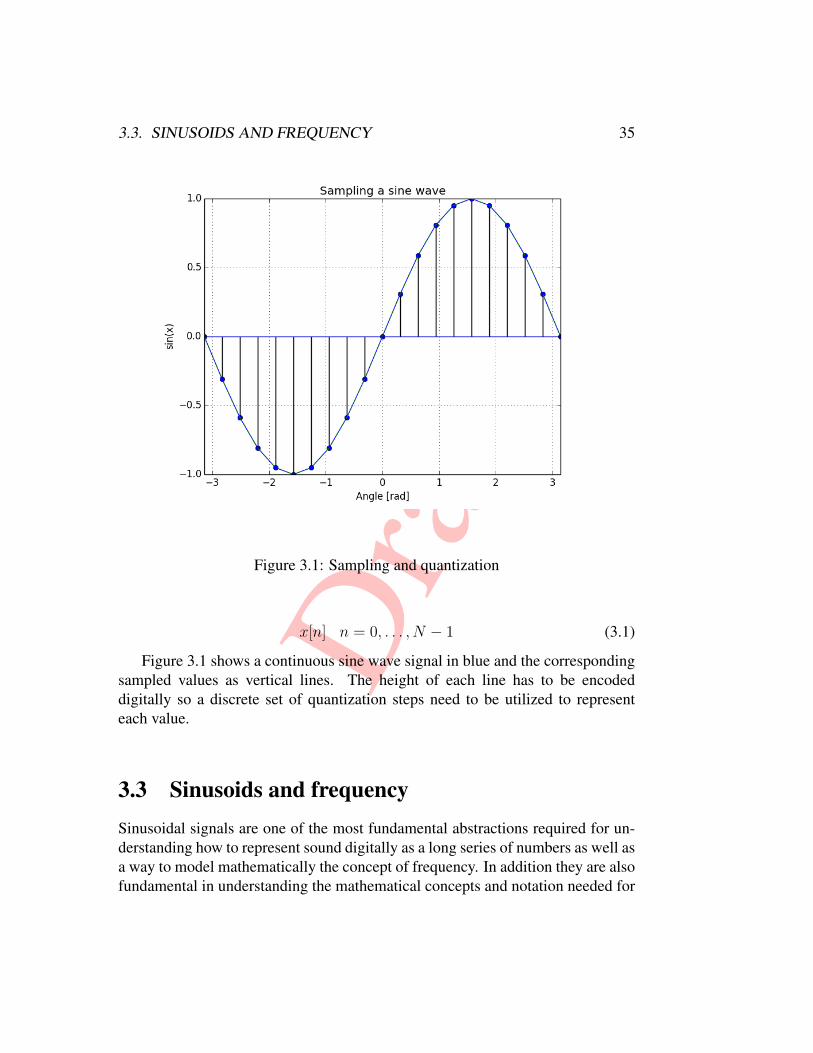
Dra
ft
3.3. SINUSOIDS AND FREQUENCY 35
Figure 3.1: Sampling and quantization
x[n] n = 0, . . . , N − 1 (3.1)
Figure 3.1 shows a continuous sine wave signal in blue and the correspondingsampled values as vertical lines. The height of each line has to be encodeddigitally so a discrete set of quantization steps need to be utilized to representeach value.
3.3 Sinusoids and frequencySinusoidal signals are one of the most fundamental abstractions required for un-derstanding how to represent sound digitally as a long series of numbers as well asa way to model mathematically the concept of frequency. In addition they are alsofundamental in understanding the mathematical concepts and notation needed for

Dra
ft
36 CHAPTER 3. AUDIO REPRESENTATIONS
analyzing and manipulating audio signals so we start our exposition by discussingsinusoids.
Most readers of this book probably have a rough intuitive understanding ofa spectrum as a way of measuring/showing the amount of different frequenciespresent in a signal. For example we know what is the effect of using a graphicequalizer to boost low frequencies. At the same time if someone is not familiarwith digital signal processing then equations such as the definition of the Fouriertransform:
X(f) =
∫ ∞−∞
x(t)e−j2πftdt (3.2)
are intimidating and hard to interpret. Frequently even students that have takencourses on the topic end up manipulating the symbols mechanically without adeeper understanding of the underlying concepts. In the following subsections wewill attempt to explain the fundamental ideas underlying spectral analysis and thenotation used to expresss them.
3.3.1 Sinusoids and phasorsSinusoidal signals are functions of a particular shape that have some rather re-markable properties. For example one of the most fundamental ideas in digitalsignal processing is that any sound we hear can be represented as a summationof sine waves. We motivate sine waves through several different complimentaryways of viewing them:
• As solutions to the differential and partial differential equations describingthe physics of simple vibrating sound generating systems and as good ap-poximation of more complex vibrating systems.
• As the only family of signals that pass in some way unchanged throughlinear time-invariant systems (LTI). More specifically passing a sine waveof a particular frequency through a LTI system will result in a sine wave ofthe same frequency possibly scaled and shift in phase i.e the basic “shape”of the signal remains the same. Many of the systems involved in the pro-duction, propagation and sensing of sound can be modeled with reasonableaccuracy as linear time-invariant systems and understanding their responseto sine waves can be very informative about what these systems do.
Dra
ft
3.3. SINUSOIDS AND FREQUENCY 37
• As phasors (rotating vectors) they form an expressive notation that helpsintuition and understanding of many fundamental digital signal processingconcepts.
• As the basis functions of the Fourier Transform which can be used to repre-sent any periodic signal as a summation of elementary sinusoidal signals.
The term sinusoid is used to describe a family of elementary signals that havea particular shape/pattern of repetition. The sine wave x(t) = sin(ωt) and thecosine wave x(t) = cosin(ωt) are particular examples of sinusoids that can bedescribed by the more general equation:
x(t) = sin(ωt+ φ) (3.3)
where ω is the frequency and φ is the phase. There is an infite number of continu-ous periodic signals that belong to the sinusoid family but essentially they all havethe same shape. Each particular member is characterized by three numbers: theamplitude which encodes the maximum and minimum value of the oscillation, thefrequency which encodes the period of repetition, and the phase which encodesthe initial position at time t = 0. Figure 3.2 shows two sinusoid signals over atime interval of 3 seconds. The first signal (S1) has an amplitude of 7 in arbitraryunits, a frequency of 2Hz, and phase equal to 0. The second signal (S2) has anamplitude of 4, a frequency of 3Hzx, and a phase equal to π
4. The two sinusoids
are also shown superimposed (S1,S2) and their summation is also plotted (S1+S2).
3.3.2 The physics of a simple vibrating systemMusic consists of a mixture of sounds many of which are periodic and are pro-duced by musical instruments. Sound is generated by vibrations so a good placeto start is on of the simplest systems in physics that can vibrate. Let’s considerstriking a metal rod such as the tine of a tuning fork or hitting a ruler that isclamped with a hand on a table. Ther ruler deforms when it is stuck, then aforce restores it briefly to it’s original shape. However it still has inertia andit overshoot the resting position by deforming in the opposite direction. Thisoscillatory pattern repeats causing the surrounding air molecules to move and theresulting air pressure waves reach our ears as sound. The vibration at any timeis caused by the balance between two factors: the force that tends to restore theshape to equilibrium, and the intertia that tends to make it overshoot. This type

Dra
ft
38 CHAPTER 3. AUDIO REPRESENTATIONS
Figure 3.2: Simple sinusoids
of motion is called simple harmonic motion and the equation describing it can bederived from simple physics.
At any time t during the vibration Newton’s second law of motion applies:the restoring force produces an acceleration proportional to to that force. Therestoring force caused by the deformation tries to restore the ruler to its originalposition therefore acts in a direction opposite to the displacement x and for smallamounts of deformation its relation to the displacement can be considered linear.This can be written as follows:
F = ma = −kx (3.4)
Because acceleration is the second derivative with respect to the time variablet we can rewrite this equation as:
Dra
ft
3.3. SINUSOIDS AND FREQUENCY 39
d2x
dt2= −(k/m)x (3.5)
where m is the mass, k is the stiffness, x is the displacement from the restingposition and t is time. Now we need to figure out a particular function or familyof functions that satisfy the equation above. From calculus we know that thederivatives and second derivatives of the sine and cosine functions of t are alsosinusoids:
d
dtsin(ωt) = ω cos(ωt)
d2
dt2sin(ωt) = −ω2 sin(ωt) (3.6)
d
dtcos(ωt) = −ωsin(ωt)
d2
dt2cos(ωt) = −ω2 cos(ωt) (3.7)
where ω is the frequency of oscillation. The only difference between the functionssin(ωt) and cos(ωt) is that they differ by a delay/time shift but essentially theyhave the same shape. The term sinusoid will be used when it is not importantto distinguish between sine and cosine. As can be seen both of these functionsof t satisfy equation 3.5 that characterizes simple harmonic motion. It is alsostraightforward to show that the equation is satisfied by any sinusoid with anarbitrary phase φ of the following form:
x(t) = sin(ωt+ φ) (3.8)
Therefore sinusoidal signals arise as solutions to equations that that character-ize simple (or simplified) sources of sound vibration such as a tuning fork.
3.3.3 Linear Time Invariant SystemsA general system takes as input one or more input signals and produces as out-put one or more output signals. We will focus on single input/single output(SISO) systems as they can be used for many operations on audio signals. Inaddition more complicated MIMO (multiple-input, multiple-output) systems canbe assembled by connecting elementary SISO systems together in processingnetworks. A very important class of SISO systems are the Linear Time-Invariant(LTI) systems because the can be used to model many physical processes andthe LTI property makes them easier to handle mathematically. Let’s use thefollowing notation: y(t) is the system output, S is the system and x(t) is the
Dra
ft
40 CHAPTER 3. AUDIO REPRESENTATIONS
system input. Linearity means that one can calculate the output of the systemto the sum of two input signals by summing the system outputs for each inputsignal individually. Formally if y1(t) = S[x1(t)] and y2(t) = S[x2(t)] thenS[x1(t)+x2(t)] = ysum(t) = y1(t)+y2(t). Time invariance (or shift invariance indiscrete systems) means that the output of the system given an input shifted in timeis the same as the output of the system of the original unshifted input signal shiftedby the same amount. Formally if y(t) = S[x(t)] then S[x(t − t0)] = y(t − t0)where t0 is the amount of shifting in time. As we will see shortly frequently we canexpress complicated signals of interest as linear combinations of more elementarysignals. When processing such compicated signals through a LTI system we cananalyze its response simply by looking at how it responds to the elementary signalsand then combining these individual responses.
Now comes the interesting part which is what happens when a sinusoidalsignal is used as input to a LTI system. It turns out that no matter what LTI systemis used, the output not only will also be a sinusoidal signal but also have thesame frequency as the original input sinusoid. By extension if the input to a LTIsystem is a linear combination of sinusoidal components of certain frequencies,no new frequencies will be introduced in the output. Therefore we can completelycharacterize a LTI system by how it responds to elementary sinusoidal signals.Several processes in sound generation and perception can be modelled by LTIsystems. Examples include the resonant cavities of musical instruments such asthe body of a guitar, parts of the human hearing process such as the the effect ofthe outer ear, and acoustic spaces such as a concert hall. So far we have motivatedsinusoidal signals from physics of simple vibrations and from LTI systems. Nowwe look into the mathematical notation and concepts that we will need.
3.3.4 Complex NumbersA good intuitive understanding of sinusoidal signals and the mathematical no-tation conventions used to represent and manipulate them, is important in orderto understand how time-frequency representations work. The notation conven-tions typically used are based on complex numbers which can intimidate readerswithout a background in digital signal processing and mathematics. Thinking ofsinusoidal signals as vectors rotating at a constant speed on the plane, rather thanas single-valued signals that go up and down will help us demystify the complexnumber notation as well as be able to explain interesting properties geometricallyrather than algebraically.

Dra
ft
3.3. SINUSOIDS AND FREQUENCY 41
Figure 3.3: Cosine and sine projections of a vector on the unit circle (XXX Figure
needs to be redone)
Dra
ft
42 CHAPTER 3. AUDIO REPRESENTATIONS
Figure 3.3 shows how the projection of a vector on the unit cycle with angleθ onto the x-axis is the cosine of the angle and the projection onto the y-axis isthe sine of the angle. If that vector rotates at constant speed and we plot the x andy axis projections over time the resulting single-valued waveforms are a cosinewave and a sine wave respectively. So we can think of any sine wave as a rotatingclock hand or the spoke of bicycle wheel.
Complex numbers provide an elegant notation system for manipulating rotat-ing vectors. Any vector with coordinates x and y is notated as the complex numberx + jy. The x part is called the real part and the part with the weird j factor iscalled the imaginary part. Typically j is defined as
√−1. This somewhat strange
looking definition makes much more sense if we think of j as meaning rotate by π2
(counter-clockwise). Starting from the real number 1 (with 0 imaginary part) twosuccesive rotations bring us to the real number −1 hence j2 = −1. This shouldmake it clear that there is nothing imaginary or complex about j if it is consideredas a rotation.
In terms of addition complex numbers behave exactly as vectors. The x-coordinate of the sum of two vectors is the sum of the x-coordinates and the y-coordinate of the sum of two vectors is the sume of the y-coordinates. Similarlythe real part of the sum is the sum of the real parts and the imaginary part of thesum is the sum of the imaginary parts. The expressive power of complex numbersshows up when they are multiplied. We define multiplication using standardalgebra and taking care to replace j2 with −1 whenever we need to. Supposewe want to multiple the complex number a+ jb with the complex number c+ jd.The result is the following complex number:
(a+ jb) ∗ (c+ jd) = ac+ jbc+ jad+ j2bd = (ac− bd) + j(ad+ bc) (3.9)
Notice that the use of j is simply a convenient notation so that we can manipulateexpressions of complex numbers using our familiar addition and multiplicationskills for real numbers. When writing computer code j is not needed and wecould write the definition directly as:
S.re = A.re * B.re - A.im * B.im
S.im = A.re * B.im + B.re * A.im
In order to understand the effect of complex number multiplication we needto think of complex numbers as vectors in polar form. The lenght of the complex

Dra
ft
3.3. SINUSOIDS AND FREQUENCY 43
number c = a + jb is called the magnitude, is written as |c|, and is the Euclideandistance from the origin interpreting a and b as the x and y coordinates:
R = |c| =√a2 + b2 (3.10)
The angle with the real axis is often called its argument and is given by:
θ = ARG(c) = arctan(b/a) (3.11)
Based on these definitions a complex number can be notated as R∠θ. You canvisualize this as scaling the unit vector on the real-axis by R and then rotatingthe result counter-clockwise by angle theta in order to get to a particular point onthe 2D plane. As examples the complex number 1 + j0 is 1∠0 and the complexnumber 0 + j1 is 1∠π
2. We can easily go back to cartesian coordinates based on
the relations shown in Figure 3.3.
a = R cos θ b = R sin θ (3.12)
When complex numbers are represented in polar form their multiplication hasa clear geometric interpretation. The magnitudes are multiplied and the anglesare added i.e the product of R1∠θ1 and R2∠θ2 is R1R2∠(θ1 + θ2). Visuallymultiplication by a compex number is simply a rotation and scaling operation.I hope that after reading this section you can see complex numbers are not ascomplex if viewed from the right angle.
3.3.5 PhasorsLet’s return to our representation of sinusoids as rotating vectors with constantspeed and try to use what we have learned about complex numbers for expressingthem mathematically. A complex sinusoid can be simply notated as:
cos (ωt) + j sin (ωt) (3.13)
where ω is the frequency in radians per second. Every time the time t changes therotating vectors moves around the circle. For example, when the change is 2π
ωthe
argument ωt changes by 2π radians and the sinusoidal signal goes through onecycle.
Another way to view this process is that the rotating vector that represents asinusoid is just a single fixed complex number raised to progressively higher and

Dra
ft
44 CHAPTER 3. AUDIO REPRESENTATIONS
higher powers as time goes by. As we have seen complex number multiplicationcan be interpreted as a rotation so raising a complex number to an integer powercorresponds to moving the phasor around the circle in discrete steps. By makingthe power continuous and a function of time we can model a continuous rotation.More specifically we can notate our rotating phasor as a function of continuousangle (assuming unit magnitude):
E(θ) = Cθ = cos θ + j sin θ = 1∠θ (3.14)
whereθ = ωt (3.15)
We can easily calculate the derivative of this complex function E(θ) with respectto θ:
dE(θ)
dθ= − sin θ + j cos(θ) = jE(θ) (3.16)
As can be seen this is a function for which the derivative is proportional tothe original function and from calculus we know that that only the exponentialfunction has this property so we can write our function E(θ) as:
E(θ) = ejθ (3.17)
So now we can express the fact that a rotating vector arising from simpleharmonic motion can be notated as a complex number raised to higher and higherpowers using the famous Euler formula named after the Swiss mathematicianLeonard Euler (1707-1783):
ejθ = cos θ + j sin(θ) (3.18)
We can make the relation to time and frequency more explicit by replacing θ witheither ωt or 2πft :
ejωt = cosωt+ j sin(ωt) (3.19)
Hopefully after this exposition the complex number notation used in the def-inition of various frequency transforms will not look as intimidating. Anotherpossible viewpoint is to simply consider the use of exponentials as a notationconvention that allows us to express complex number multiplication using theregular rules we expect from exponents. Using this convention the multiplicationof two complex numbers c1 and c2 can be written as:
Dra
ft
3.3. SINUSOIDS AND FREQUENCY 45
c1 · c2 = R1ejθ1R2e
jθ2 = R1R2ej(θ1+θ2) (3.20)
We end this subsection by returning to the geometric view of phasors as vec-tors rotating at constant speed and using it to illustrate intuitive explanations ofsome important properties of sinusoidal signals.
XXX geometric phasor descriptions of negative frequency and cancelling ofthe imaginary part, adding sinusoids of the same frequency but with differentamplitude and phase, aliasing and associated figures XXX
3.3.6 Time-Frequency Representations
A large number of organisms including humans are capable of both producing anddetecting sound (variations in air pressure). The two most important questionsa listener needs to answer regarding any sound are when it happened and whatproduced it. One important cue about the origin of a sound is the rate of theperiodic variation in air pressure. For example it is unlikely (actually physicallyimpossible) that a low loud rumbling sound will come from a tiny bird. Thereforeit is hardly surprising that most animal auditory systems are structured so that atthe most basic level they can differentiate between sounds happening at differenttimes and having different rates of vibration (frequencies). Without going intodetails in most mammallian auditory systems sounds with different frequenciesexcite different groups of neurons (inner hair cells) attached to a membrane (thebasilar membrane) that performs a type of frequency analysis; a given place alongthe basilar membrane responds more strongly to a sinusoidal vibration of a partic-ular frequency. At the same time a given place along the basilar membrane willalso react to other frequencies to a lesser degree and further mechanisms related totiming are used to better resolve these frequencies. Furthermore various structuralfeatures of the auditory cortex (the part of the brain that deals with understandingsound) are “tonotopically” organized. When excited by a sine wave of increasingfrequency the excitation on the cortex moves continuously along a curved path.So there is something fundamental about frequency in the response of the brain tosound, right up to the highest level, the auditory cortex.
Dra
ft
46 CHAPTER 3. AUDIO REPRESENTATIONS
3.3.7 Frequency Domain Representations
A frequent and elegant approach to representing audio signals is to express themas weighted mixtures of elementary building blocks (basis functions) which canbe thought of as simple prototypical signals. Then the representation essentiallyconsists of the weights of the mixture. Audio signal representations computedusing the same set of basis functions can be then analyzed and compared simplyby considering the weights of the mixture. A common strategy in digital signalprocessing it to take advantage of a strategy called superposition. In superpo-sition the signal being processed is decomposed into simple components, eachcomponent is processed separately and the results are reunited. Linear systemsare typically required for superposition to work. As we have already discussed inorder to extract information from music audio signals the audio representationmust somehow encode time and frequency. By analyzing the audio signal insmall chunks the representation becomes dependent on time and by utilizing basisfunctions that correspond to different frequency the weights of the mixture encodefrequency.
There are four commonly used variants of frequency domain representations:the Fourier series, the Discrete Fourier Transform (DFT), the z-transform, and theclassical Fourier transform. The intuition behind all of them is similar. The mainidea is to express the signals of interest as weighted mixture of elementary signals;as you probably expect these will be some form of sinusoidal signals i.e phasors.Armed with our knowledge of sinusoidal signals and how they can be viewed asphasors and notated using complex numbers we are ready to understand some ofthe most fundamental concepts in digital signal processing.
Coordinate systems
The weights of a mixture of elementary signals can be viewed as coordinates in asignal space spanned by these elementary signals in an analogous way to how thespatial coordinates of a point in space can viewed as the weights that are neededto combine the unit-length basis vectors corresponding to each axis. For examplea vector ν in three-dimensional space can be written as:
ν = νxx + νyy + νzz (3.21)
which can be interpreted as the fact that any vector in the three-dimensional spacecan be represented as a weighted combination of three parts: a vector in the x-
Dra
ft
3.3. SINUSOIDS AND FREQUENCY 47
direction of length νx, a vector in the y-direction of length νy and a vector in thez direction of length νz. The three unit length vectors in the coordinate directionsx,y, z are called a basis for the three dimensional space and the numbers νx, νy, νzare called the projections of vector ν onto the respective basis elements. We candenote the projection of a vector ν onto another vector u by ν < ν, u > in whichcase:
νx = 〈ν,x〉νy = 〈ν,y〉νz = 〈ν, z〉
The projection 〈ν, υ〉 is also called the inner product of ν and υ and can bedefined as the sum of products of like coordinates (when the vector has coordinatevalues that are complex numbers the coordinates of the second vector need to beconjugated):
〈ν, υ〉 = νxυ∗x + νyυ
∗y + νzυ
∗z (3.22)
or more generally:〈ν, υ〉 =
∑i
νiυ∗i (3.23)
The projection/inner product follows a distributive law and is symmetric whichmeans that:
〈ν + υ, ω〉 = 〈ν, ω〉+ 〈υ, ω〉 (3.24)
〈ν, υ〉 = 〈υ, ν〉 (3.25)
Also notice that the projection of a vector onto itself (or equivalently the innerproduct of a vector with itself) is the square of the length of the vector (noticehow the complex conjugate in the definition of the inner product is required tomake this true when the coordinates are complex numbers):
〈ν, ν〉 = |νx|2 + |νy|2 + |νz|2 (3.26)
The three coordinate basis vectors x,y, z are orthogonal to each other whichmeans that their projections onto each other are zero.
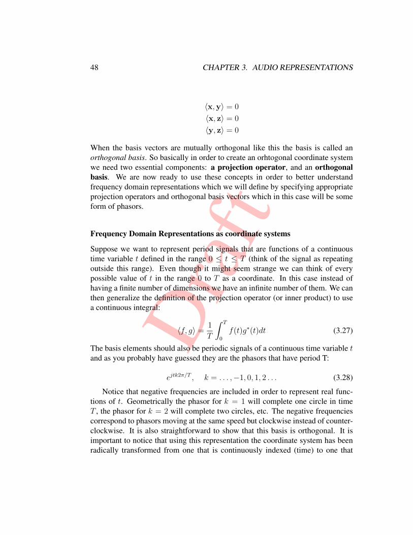
Dra
ft
48 CHAPTER 3. AUDIO REPRESENTATIONS
〈x,y〉 = 0
〈x, z〉 = 0
〈y, z〉 = 0
When the basis vectors are mutually orthogonal like this the basis is called anorthogonal basis. So basically in order to create an orhtogonal coordinate systemwe need two essential components: a projection operator, and an orthogonalbasis. We are now ready to use these concepts in order to better understandfrequency domain representations which we will define by specifying appropriateprojection operators and orthogonal basis vectors which in this case will be someform of phasors.
Frequency Domain Representations as coordinate systems
Suppose we want to represent period signals that are functions of a continuoustime variable t defined in the range 0 ≤ t ≤ T (think of the signal as repeatingoutside this range). Even though it might seem strange we can think of everypossible value of t in the range 0 to T as a coordinate. In this case instead ofhaving a finite number of dimensions we have an infinite number of them. We canthen generalize the definition of the projection operator (or inner product) to usea continuous integral:
〈f, g〉 =1
T
∫ T
0
f(t)g∗(t)dt (3.27)
The basis elements should also be periodic signals of a continuous time variable tand as you probably have guessed they are the phasors that have period T:
ejtk2π/T , k = . . . ,−1, 0, 1, 2 . . . (3.28)
Notice that negative frequencies are included in order to represent real func-tions of t. Geometrically the phasor for k = 1 will complete one circle in timeT , the phasor for k = 2 will complete two circles, etc. The negative frequenciescorrespond to phasors moving at the same speed but clockwise instead of counter-clockwise. It is also straightforward to show that this basis is orthogonal. It isimportant to notice that using this representation the coordinate system has beenradically transformed from one that is continuously indexed (time) to one that

Dra
ft
3.3. SINUSOIDS AND FREQUENCY 49
is discretely indexed (the phasor basis indexed by integers). Although there aresome mathematic restrictions it is remarkable that this works.
Based on these two definition of projection operator and basis functions wecan now express any periodic function in terms of the basis:
f(t) =∞∑−∞
Ckejkt2π/T (3.29)
The complex coefficient Ck can be thought of as the coordinate in the “direc-tion” of the phasor ejkt2π/T or the amount of the frequency k2π/T . Equation 3.29is called the Fourier Series of f(t) and the values CK are called the spectrumof the periodic signal f(t). To find the Fourier coefficients Ck we can simplyproject f(t) on the kth basis element (having a bad memory I always rely on thedefinition of the inner product with the complex conjugate to determine the signof the exponent in frequency transforms):
Ck = 〈f(t), ejkt2π/T 〉 =1
T
∫ T
0
f(t)e−jkt2π/Tdt (3.30)
Notice that when f(t) is a real (as is the case for audio signals) there is a verysimple relationship between the coefficients for negative and positive frequencies:
Ck = C∗−k (3.31)
3.3.8 Discrete Fourier TransformThe Fourier Series representation transforms periodic signals in a continuous timedomain to an infinite discrete frequency domain. Therefore it is not directlyusable when processing digital signals. The transform that is needed is calledthe Discrete Fourier Transform (DFT). It transforms a finite discrete time domainsignal (or an array of numbers in computer parlance) to a finite discrete frequencydomain signal (also an array of numbers). The DFT arguably the most widelyused transform in digital signal processing and as an extension in MIR. In partthis because of a very fast algorithm for computing it that is called the FastFourier Transform (FFT). Even though the tecnique was first discovered by Gaussin 1805 it became widely used in its current form through the work of Cooleyand Tukey. In the published literature frequently the terms DFT and FFT are usedinterchangeably but it is good to keep in mind the the DFT refers to the transform

Dra
ft
50 CHAPTER 3. AUDIO REPRESENTATIONS
whereas the FFT refers to a fast algorithm for computing it. Similarly to howthe Fourier Series was presented we define the DFT by specifying a projectionoperator and a set of basis functions. As probably expected the projection operatoris the standard inner product between vectors of complex numbers:
〈x, y〉 =∑i
xty∗t (3.32)
Due to aliasing frequencies of discrete-time signals are equivalent modulo thesampling frequency.
Arguably the most basic elementary basis function is the sampled sinusoidwhich forms the basis of the Discrete Fourier Transform and the Short TimeFourier Transform (STFT). The STFT forms the foundation of most proposedalgorithms for the analysis of audio signals and music. So our description ofaudio representations begins with the sound of a sinusoid.
Audio Examples Source Code (Marsyas/Matlab) Figure
3.3.9 Sampling and Quantization
3.3.10 Discrete Fourier Transform
3.3.11 Linearity, propagation, resonances
3.3.12 The Short-Time Fourier Transform
Music-humans-language-mental models-abstraction-better time modeling scales
MPEG-7 standard
“feature” is a distinctive characteristic of the data which signifies somethingto somebody.
Dra
ft
3.4. PERCEPTION-INFORMED REPRESENTATIONS 51
3.3.13 Wavelets
3.4 Perception-informed Representations
3.4.1 Auditory Filterbanks
3.4.2 Perceptual Audio Compression
3.5 Source-based Representations
LPC
3.6 Further Reading
The theory behind the audio representations used in music information retrievalforms the field of Digital Signal Processing (DSP). There are many excellent DSPbooks. The following list consists of a few of my own personal preferences ratherthan any attempt at a comprehensive catalog. The DSP Primer by Ken Steiglitz [?]is my favorite beginner book as it stresses intuition and has a strong emphasis onmusic. The classic book by Oppenheim and Schafer [?] is the essential referencefor anyone needing a deeper understanding of signal processing.
Digital Signal Processing: A Practical Guide for Engineers and Scientists[Paperback] Steven Smith (Author)
Paperback: 650 pages Publisher: Newnes; Book and CD ROM edition (Novem-ber 6, 2002) Language: English ISBN-10: 075067444X ISBN-13: 978-0750674447Product Dimensions: 9.9 x 7.2 x 1.2 inches Shipping Weight: 2.6 pounds
Understanding Digital Signal Processing (2nd Edition) [Hardcover] RichardG. Lyons (Author) Hardcover: 688 pages Publisher: Prentice Hall; 2 edition(March 25, 2004) Language: English ISBN-10: 0131089897 ISBN-13: 978-0131089891
Hardcover: 1120 pages Publisher: Prentice Hall; 3 edition (August 28, 2009)Language: English ISBN-10: 0131988425 ISBN-13: 978-0131988422 Product
Dra
ft
52 CHAPTER 3. AUDIO REPRESENTATIONS
Dimensions: 9.3 x 7.5 x 1.7 inches Shipping Weight: 4.2 pounds (View shippingrates and policies)
Discrete-Time Signal Processing (3rd Edition) (Prentice Hall Signal Process-ing) [Hardcover] Alan V. Oppenheim (Author), Ronald W. Schafer (Author)
Problems1. Show that a sinusoidal signal with any phase angle satisfies equation 3.5
2. Show that the basis fuctions for the Fourier Series are orthogonal using theappropriate definition of an inner product.

Dra
ftChapter 4
Music Representations
Music is an ephemeral activity and for most of human history it only existed whileit was created. The only way it was represented was in the mental memories ofmusicians. Although such mental representations can actually be quite abstractand effective in terms of retrieval their workings are a mystery and not easityunderstood through introspection. For example, a musician might easily recognizea tune from a badly rendered melodic fragment sung by an audience member orbe able to play from memory a highly complex piece of music. However in mostcases it is impossible or very hard to describe how these tasks are accomplished.The use of external symbolic representations to communicate and store informa-tion was a major technological advancement in human history. Several writingsystems were developed codifying different types of information the most wellknown being logistical/accounting information, concepts/words (hieroglyphics)and phonemes/sounds (alphabet). Gradually symbolic representations for cod-ifying different aspects of music were developed with western common musicnotation being probably the most well known and used example today. Musiciansspend many hours learning and studying how to codify music in scores and howto perform music written as a score. Even though a full music education isnot required to work on music information retrieval a basic understanding ofhow scores codify music is essential in comprehending several tasks that havebeen investigated in MIR. This chapter is an overview of the basic music theory,concepts and abstractions involved when representing music symbolically. For
53
Dra
ft
54 CHAPTER 4. MUSIC REPRESENTATIONS
readers with a formal music background this material is probably familiar andshould be skipped as needed.
The “dimensions” of time and frequency are also fundamental in understand-ing music from cultures from around the world and throughout history. Pitchrefers to the subjective perception of frequency by humans. It is also important tokeep in mind that a periodic sound will have a clear pitch only if it has sufficientduration. Much of our knowledge of pitch perception comes from psychophysicsthe psychology discipline that investigates the relationship between physical stim-uli and their subjective perception. For example an important concept in psy-chophysics is the idea of “just noticable difference” (JND) which is the differencein physical stimuli that subjects can not detect reliably. In a typical experimen-tal setup for pitch perception the subject is played two sine waves of differentfrequencies and is asked to say whether they are the same or not. Based onsimilar experiments it can be shown that the total number of perceptible pitch stepsin the range of human hearing is approximately 1400 (several factors includingindividual differences, intensity, duration and timbre can affect this number).
Categorical perception occurs when the continuous stimuli that reach our senseorgans is sorted out by our brains into distinct categories whose members come toresemble more one another than they resemble members of the other categories.The canonical example of categorical perception is how we perceive colors. Inphysical terms colors differ only in their wavelength which gets shorter across thespectrum of visible colors. However we perceive discrete categories such as red,orange and green. Similar categorical perception can be observed in speech andmore importantly for our purposes in the perception of pitch.
Many music cultures utilize some form of division of the pitch continuum indiscrete categories. Some of these devisions are more formalized while others aremore subjective and vary among culture, instrument and performers. An intervalbetween two sounds is their spacing in pitch. Most humans have categoricalperception of pitch intervals.The identity of a melody (sequence of notes) like“Twinkle, Twinkle Little Star” is based on a sequence of pitch intervals and is toa large extent not affected by the frequency of the starting note. The most fun-damental interval is the “octave” or a doubling in frequency which is recognizedby most music traditions. Tuning systems are formalized theories that describehow categorical pitch intervals are formed. All tuning systems are affected by thephysics of sound production and perception but they are also affected by musictraditions and tuning pecularities of the instruments used in those traditions.
Pitch intervals are perceived as ratios of frequencies so that an octave above440 Hz (the frequency used today for tuning in most western classical music)
Dra
ft
4.1. COMMON MUSIC NOTATION 55
would be 880 Hz and an octave above 880 Hz would be 1760 Hz. Most tuningsystems can be viewed as different ways of subdividing the octave (the intervalcorresponding to a frequency ratio of two).
Tuning systems and their relations with timbre and acoustics are a fascinatingtopic however for the purposes of this book we will only consider two well knownvariants: Pythagorean tuning and Equal Temperement. More details about tuningsystems can be found in Sethares [?].
4.0.1 Music Representations through HistoryMusic information to this day is largely orally transmitted. Most humans can singand recognize a large variety of different songs and tunes even if a page of musicnotation means nothing to them.
Through ancient times different written music representations have been used.Although the amount of information represented differs in each case it is notsufficient to capture all the details and nuances of a music performance.
4.1 Common Music Notation
4.2 Music Theoryintervals, scales, chords, cadences
4.3 Graphical Score Representations
4.4 MIDI
4.5 MusicXML[37] [84] [?] [48] [60]

Dra
ft
56 CHAPTER 4. MUSIC REPRESENTATIONS

Dra
ftChapter 5
Feature Extraction
Audio feature extraction forms the foundation for any type of music data mining.It is the process of distilling the huge amounts of raw audio data into muchmore compact representations that capture higher level information about theunderlying musical content. As such it is much more specific to music than thedata mining processes that typically follow it.
A common way of grouping audio features (or descriptors as they are some-times called) is based on the type of information they are attempting to capture[94]. On an abstract level one can identify different high level aspects of a musicrecording. The hierarchical organization in time is refered to as rhythm and thehierarchical organization in frequency or pitch is refered to as harmony. Timbreis the quality that distinguishes sounds of the same pitch and loudness generatedby different methods of sound production. We will use the term timbral textureto refer to the more general quality of the mixture of sounds present in music thatis independent of rhythm and harmony. For example the same piece of notatedmusic played at the same tempo by a string quartet and a saxophone quartet wouldhave different timbral texture characteristics in each configuration. In this chaptervarious audio feature extraction methods that attempt to capture these three basicaspects of musical information are reviewed. Some additional audio features thatcover other aspects of musical information are also briefly described. The chapterends with a short description of audio genre classification as a canonical casestudy of how audio featue extraction can be used as well as some references tofreely available software that can be used for audio feature extraction. Audio
57

Dra
ft
58 CHAPTER 5. FEATURE EXTRACTION
feature extraction is a big topic and it would be impossible to cover it fully inthis chapter. Although our coverage is not complete we believe we describemost of the common audio feature extraction approaches and the bibliographyis representative of the “state of the art” in this area in 2010.
5.1 Timbral Texture FeaturesFeatures representating timbral information have been the most widely used audiofeatures and ones that have so far provided the best results when used in isola-tion. Another factor in their popularity is their long history in the area of speechrecognition. There are many variations in timbral feature extraction but mostproposed systems follow a common general process. First some form of time-frequency analysis such as the STFT is performed followed by summarizationsteps that result in a feature vector of significantly smaller dimensionality. Asimilar approach can be used with other time-frequency represenations.
5.1.1 Spectral FeaturesSpectral features are directly computed on the magnitude spectrum and attemptto summarize information about the general characteristics of the distributionof energy across frequencies. They have been motivated by research in timbreperception of isolated notes of instruments [41]. The spectral centroid is definedas the center of gravity of the spectrum and is correlated with the perceived“brightness” of the sound. It is defined as:
Cn =
∑N−1k=0 |X[k]|nk∑N−1
k=0 k(5.1)
where n is the frame number to be analyzed, k is the frequency bin number and|X(k)|n is the corresponding magnitude spectrum.
The spectral rolloff is defined as the frequency Rn below which 85% of theenergy distribution of the magnitude spectrum is concentrated:
Rn−1∑n=0
= 0.85 ∗N−1∑n=0
|X[k]|n (5.2)
Dra
ft
5.1. TIMBRAL TEXTURE FEATURES 59
5.1.2 Mel-Frequency Cepstral Coefficients
The Mel-Frequency Cepstral Coefficients MFCC [22] are the most common repre-sentation used in automatic speech recognition systems and have been frequentlyused for music modeling. Their computation consists of 3 stages: 1) Mel-scalefilterbank 2) Log energy computation 3) Discrete Cosine Transform.
A computationally inexpensive method of computing a filterbank is to performthe filtering by grouping STFT bins using triangular windows with specific centerfrequencies and bandwidths. The result is a single energy value per SFTFT framecorresponding to the output of each subband. The most common implementationof MFCC is caclulated using 13 linearly spaced filters separated by 133.33 Hzbetween their center frequencies, followed by 27 log-spaced filters (separated bya factor of 1.0711703 in frequency) resulting in 40 filterbank values for each STFTframe.
The next step consists of computing the logarithm of the magnitude of each ofthe filterbank outputs. This can be viewed as a simple step of dynamic compres-sion, making feature extraction less sensitive to variations in dynamics.
The final step consists of reducing the dimensionality of the 40 filterbankoutputs by performing a Discrete Cosine Transform (DCT) which is similar to theDiscrete Fourier Transform but uses only real numbers. It expresses a finite set ofvalues in terms of a sum of cosine functions oscillating at difference frequencies.The DCT is used frequently in compression applications because for typical sig-nals of intererst in tends to concentrate most of the signal information in few ofthe lower frequency components and therefore higher frequency components canbe discarded for compression purposes. In the “classic” MFCC implementationthe lower 13 coefficients are retained after transforming the 40 logarithmicallycompressed Mel filterbank outputs.
[68]
5.1.3 Other Timbral Features
There have been many other features proposed to describe short-term timbralinformation. In this subsection we briefly mention them and provide citations towhere the details of their calculation can be found. Time domain zero-crossingscan be used to measure how noisy is the signal and also somewhat correlate tohigh frequency content [94, 10]. Spectral bandwidth [10, 30, 69] and octavebased spectral contrast [52, 69] are other features that attempt to summarize the

Dra
ft
60 CHAPTER 5. FEATURE EXTRACTION
magnitude spectrum. The spectral flatness measure and spectral crest factor [1]are low level descriptors proposed in the context of the MPEG-7 standard [15].
[67]
Daubechies Wavelet Coefficient Histogram is a technique for audio featureextraction based on the Discrete Wavelet Transform (DWT) [63]. It is applied in3 seconds of audio using the db8 Daubechies wavelet filter [21] with seven levelsof decomposition. After the decomposition, the histograms of the coefficients ineach band are calculated. Finally each histogram is characterized by its mean,variance and skewness as well as the subband energy defined as the mean of theabsolute coefficient values. The result is 7 (subbands) * 4 (quantities per subband)= 28 features.
One of the major innovations that enabled the explosive growth of musicrepresented digitally is perceptual audio compression [77]. Audio compression isfrequently used to reduce the high data requirements of audio and music. Audiodata does not compress well using generic data compression algorithms so spe-cialized algorithms have been developed. The majority of audio coding algorithmsare lossy meaning that the original data can not be reconstructed exactly from thecompressed signal. They are frequently based on some form of time-frequencyrepresentation and they achieve compression by allocating different number ofbits to different parts of the signal. One of the key innovations in audio coding isthe use of psychoacoustics (i.e the scientific study of sound perception by humans)to guide this process so that any artifacts introduced by the compression are notperceptible.
There has been some interest in computing audio features directly in the com-pressed domain as part of the decompression process. Essentially this takes advan-tage of the fact that a type of time-frequency analysis has already been performedfor encoding purposes and it is not necessary to repeat it after decompression. Thetype of features used are very similar to the ones we have described except for thefact that they are computed directly on the compressed data. Early works mainlyfocused on the MPEG audio compression standard and the extraction of timbraltexture features [93, 82]. More recently the use of newer sparse overcompleterepresenations as the basis for audio feature extraction has been explored [28]covering timbral texture, rhythmic content and pitch content.

Dra
ft
5.1. TIMBRAL TEXTURE FEATURES 61
5.1.4 Temporal Summarization
The features that have been described so far characterize the content of a veryshort segment of music audio (typically around 20-40 milliseconds) and can beviewed as different ways of summarizing frequency information. Frequently asecond step of temporal summarization is performed to characterize the evolutionof the feature vectors over a longer time frame of around 0.5 to 1 seconds. Wecan define a “texture” window TM [n] of size M corresponding to analysis framen as the sequence of the previous M − 1 computed feature vectors including thefeature vector corresponding to n.
TM [n] = F [n−M + 1]...F [n] (5.3)
Temporal integration is performed by summarizing the information containedin the texture window to a single feature vector. In other words the sequenceof M past feature vectors is “collapsed” to a single feature vector. At the oneextreme, the texture window can be advanced by one analysis frame at a time inwhich case the resulting sequence of temporally summarized feature vectors hasthe same sampling rate as the original sequence of feature vectors [94]. At theother extreme temporal integration can be performed across the entire length ofthe audio clip of interest resulting in a single feature vector representing the clip(sometimes such features are termed song-level [71] or aggregate features [10]).Figure 5.1 shows schematically a typical feature extraction process starting witha time-frequency representation based on the STFT, followed by the calculationof MFCC (frequency) summarization and ending with summarization of the re-sulting feature vector sequence over the texture window.
The is no consistent terminology describing temporal summarization. Termsthat have been used include: dynamic features [81, 72] , aggregate features [10],temporal statistics [30], temporal feature integration [74], fluctuation patterns[83], and modulation features [59]. More recently the term pooling has also beenused [?].
Statistical moments such as the mean, standard deviation and the covariancematrix can be used to summarize the sequence of feature vectors over the texturewindow into a single vector. For example a common approach is to computethe means and variances (or standard deviations) of each feature over the texturewindow [94]. Figure 5.2 shows the original trajectory of spectral centroids overa texture window as well as the trajectory of the running mean and standarddeviation of the spectral centroid for two pieces of music.

Dra
ft
62 CHAPTER 5. FEATURE EXTRACTION
Figure 5.1: Feature extraction showing how frequency and time summarization
with a texture window can be used to extract a feature vector characterizing
timbral texture

Dra
ft
5.1. TIMBRAL TEXTURE FEATURES 63
Another alternative is to use the upper triangular part of the covariance matrixas the feature vector characterizing the texture window [71]. Such statistics cap-ture the variation of feature vectors within a texture window but do not directlyrepresent temporal information.
Another possibility is to utilize techniques from multivariate time-series mod-eling to characterize the feature vector sequence that better preserve temporalinformation. For example multivariate autoregressive models have been used tomodel temporal feature evolution [74]. The temporal evolution of the featurevectors can also be characterizing by performing frequency analysis on their tra-jectories over time and analyzing their periodicity characteristics. Such modula-tion features show how the feature vectors change over time and are typicallycalculated at rates that correspond to rhythmic events. Any method of time-frequency analysis can be used to calculate modulation features but a commonchoice is the Short-Time Fourier Transform (STFT).
As a representative example of calculating modulation frequencies we brieflydescribe the approach proposed by McKinnery and Breebart [72]. A standardMFCC computation is performed resulting in a sequence of 64 feature vectorseach with 13 dimensions characterizing a texture window of 743 milliseconds ofaudio. A power spectrum of size 64 using a DFT is calculated for each of the 13coefficients/dimesions resulting in 13 power spectra which are then summarizedin 4 frequency bands (0Hz, 1− 2Hz, 3− 15Hz, 20− 43Hz) that roughly corre-spond to musical beat rates, speech syllabic rates and modulations contributing toperceptual roughness. So the final representations for the 13x64 matrix of featurevalues of the texture window is 4x13 = 52 dimensions.
A final considerations is the the size of the texture windows and the amountof overlap between them. Although the most common approach is to use fixedwindow and hop sizes there are alternatives. Aligning texture windows to noteevents can provide more consistent timbral information [97]. In many musicanalysis applications such as cover song detection it is desired to obtain an audiofeature representation that is to some-extent tempo-invariant. One way to achievethis is using so-called beat-synchronous features which as their name implies arecalculated using estimated beat locations as boundaries [29]. Although morecommonly used with features that describe pitch content they can also be usedfor timbral texture modeling.

Dra
ft
64 CHAPTER 5. FEATURE EXTRACTION
0 100 200 300 400 500Frames
0.00
0.02
0.04
0.06
0.08
0.10
Centroid
BeatlesDebussy
(a) Centroid
0 100 200 300 400 500Frames
0.00
0.01
0.02
0.03
0.04
0.05
0.06
0.07
Centroid
BeatlesDebussy
(b) Mean Centroid over
Texture Window
0 100 200 300 400 500Frames
0.000
0.005
0.010
0.015
0.020
0.025
Centroid
BeatlesDebussy
(c) Standard Deviation
of Centroid over Texture
Window
Figure 5.2: The time evolution of audio features is important in characterizing
musical content. The time evolution of the spectral centroid for two different
30-second excerpts of music is shown in (a). The result of applying a moving
mean and standard deviation calculation over a texture window of approximately
1 second is shown in (b) and (c).
5.1.5 Song-level modeling
Frequently in music data mining the primary unit of consideration is an entiretrack or excerpt of a piece of music. The simplest and most direct type of represen-tation is a single feature vector that represents the entire piece of music under con-sideration. This is typically accomplished by temporal summarization techniquessuch as the ones described in the previous section applied to the entire sequenceof feature vectors. In some case two stages of summarization are performed: oneat the texture window level and one across the song [94]. The efffectiveness ofdifferent parameter choices and temporal summarization methods has also beenexplored [10].
In other music data mining problems the entire sequence of feature vectorsis retained. These problems typically deal with the internal structure within amusic piece rather than the relations among a collection of pieces. For examplein audio segmentation [31, 91] algorithms the locations in time where the musicalcontent changes significantly (such the transition from a singing part to an electricguitar solo) are detected. Audio structure analysis goes a step further and detects

Dra
ft
5.1. TIMBRAL TEXTURE FEATURES 65
Figure 5.3: Self Similarity Matrix using RMS contours
repeating sections of a song and their form such as the well known AABA form[20]. Sequence representations are also used in cover song detection [29].
A representation that is frequently utilized in structure analysis is the selfsimilarity matrix. This matrix is calculated by calculating pair-wise similaritiesbetween feature vectors vi and vj derived from audio analysis frames i and j.
s(i, j) = sim(vi,vj) (5.4)
where sim is a function that returns a scalar value corresponding to some notionof similarity (or symmetrically distance) between the two feature vectors. Asmusic is generally self-similarity with regular structure and repetitions which canbe revealed through the self similarity matrix.
Figure 5.3 shows an example of a self-similarity matrix calculated for a pieceof HipHop/Jazz fusion using simply energy contours (shown to the left and bottomof the Matrix). The regular structure at the beat and measure level as well as somesectioning can be observed.
The final variation in song-level representations of audio features is to modeleach music piece as a distribution of feature vectors. In this case a parametric dis-tribution form (such as a Gaussian Mixture Model [3]) is assumed and its param-eters are estimated from the sequence of feature vectos. Music data mining tasks
Dra
ft
66 CHAPTER 5. FEATURE EXTRACTION
such as classification are performed by considering distance functions betweendistributions typically modeled as mixture models such as the KL-divergence orEarth Mover Distance [71, 51].
5.2 Rhythm FeaturesAutomatically extracting information related to rhythm is also an important com-ponent of audio MIR systems and has been an active area of research for over 20years. A number of different subproblems within this area have been identifiedand explored. The most basic approach is finding the average tempo of the entirerecording which can be defined as the frequency with which a human would taptheir foot while listening to the same piece of music. The more difficult task ofbeat tracking consists of estimating time-varying tempo (frequency) as well as thelocations in time of each beat (phase). Rhythmic information is hierarchical innature and tempo is only one level of the hierarchy. Other levels frequently usedand estimated by audio MIR systems are tatum (defined as the shortest commonlyoccurring time interval), beat or tactus (the preferred human tapping tempo), andbar or measure. For some MIR applications such as automatic classification it ispossible to use a a representation that provides a salience value for every possibletempoe.g., the beat histograms described in [94]. Rhythm analysis approachescan be characterized in different ways. The first and most important distinc-tion is by the type of input: most of the earlier beat tracking algorithms used asymbolic representation while audio signals have been used more recently. Sym-bolic algorithms can still be utilized with audio signals provided an intermediatetranscription step is performedtypically audio onset detection. Another majordistinction between the algorithms is the broad approach used which includesrulebased, autocorrelative, oscillating filters, histogramming, multiple agent, andprobabilistic. A good overview of these approaches can be found in Chapter 4 ofKlapuri and Davy [43].
5.2.1 Onset Strength Signal
Frequently, the first step in rhythm feature extraction is the calculation of theonset strength signal. The goal is to calculate a signal that has high values at theonsets of musical events. By analyzing the onset strength signal to detect common

Dra
ft
5.2. RHYTHM FEATURES 67
Figure 5.4: The top panel depicts the time domain representation of a fragment
of a polyphonic jazz recording, below which is displayed its corresponding
spectrogram. The bottom panel plots both the onset detection function SF(n) (gray
line), as well as its filtered version (black line). The automatically identified onsets
are represented as vertical dotted lines.
recurring periodicities it is possible to perform tempo induction, beat tracking aswell as other more sophisticated forms of rhythm analysis. Other names used inthe literature include onset strength function and novelty curve.
The onset detection algorithm described is based on a recent tutorial article[24], where a number of onset detection algorithms were reviewed and comparedon two datasets. Dixon concluded that the use of a spectral flux detection functionfor onset detection resulted in the best performance versus complexity ratio.
The spectral flux as an onset detection function is defined as :
SF (n) =
N/2∑k=0
H(|X(n, k)| − |X(n− 1, k)|) (5.5)
where H(x) = x+|x|2
is the half-wave rectifier function, X(n, k) representsthe k-th frequency bin of the n-th frame of the power magnitude (in dB) of theshort time Fourier Transform, and N is the corresponding Hamming window size.The bottom panel of Figure 5.4 plots the values over time of the onset detectionfunction SF(n) for an jazz excerpt example.
Dra
ft
68 CHAPTER 5. FEATURE EXTRACTION
The onsets are subsequently detected from the spectral fux values by a causalpeak picking algorithm, that attempts to find local maxima as follows. A peak attime t = nH
fsis selected as an onset if it satisfies the following conditions:
SF (n) ≥ SF (k) ∀k : n− w ≤ k ≤ n+ w (5.6)
SF (n) >
∑k=n+wk=n−w SF (k)
mw + w + 1× thres+ δ (5.7)
where w = 6 is the size of the window used to find a local maximum, m = 4is a multiplier so that the mean is calculated over a larger range before the peak,thres = 2.0 is a threshold relative to the local mean that a peak must reach inorder to be sufficiently prominent to be selected as an onset, and δ = 10−20 is aresidual value to avoid false detections on silent regions of the signal. All theseparameter values were derived from preliminary experiments using a collection ofmusic signals with varying onset characteristics.
As a way to reduce the false detection rate, the onset detection function SF(n)is smoothed (see bottom panel of Figure 5.4),using a Butterworth filter definedas:
H(z) =0.1173 + 0.2347z−1 + 0.1174z−2
1− 0.8252z−1 + 0.2946z−2(5.8)
In order to avoid phase distortion (which would shift the detected onset timeaway from the SF(n) peak) the input data is filtered in both the forward and reversedirections. The result has precisely zero-phase distortion, the magnitude is thesquare of the filter’s magnitude response, and the filter order is double the orderof the filter specified in the equation above.
5.2.2 Tempo Induction and Beat TrackingMany pieces of music are structured in time on top of an underlying semi-regularsequence of pulses frequently accentuated by percussion instruments especiallyin modern popular music. The basic tempo of a piece of music is the rate ofmusical beats/pulses in time, sometimes also called the “foot-tapping” rate forobvious reasons. Tempo induction refers to the process of estimating the tempoof an audio recording. Beat tracking is the additional related problem of locatingthe positions in time of the associated beats.
In this section we describe a typical method for tempo induction as a repre-sentative example and provide pointers to additional literature in the topic. The
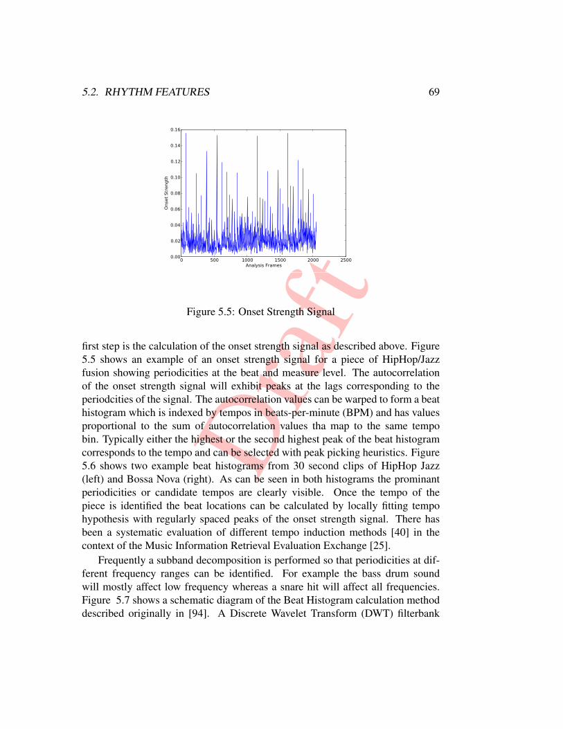
Dra
ft
5.2. RHYTHM FEATURES 69
0 500 1000 1500 2000 2500Analysis Frames
0.00
0.02
0.04
0.06
0.08
0.10
0.12
0.14
0.16
Onse
t Str
ength
Figure 5.5: Onset Strength Signal
first step is the calculation of the onset strength signal as described above. Figure5.5 shows an example of an onset strength signal for a piece of HipHop/Jazzfusion showing periodicities at the beat and measure level. The autocorrelationof the onset strength signal will exhibit peaks at the lags corresponding to theperiodcities of the signal. The autocorrelation values can be warped to form a beathistogram which is indexed by tempos in beats-per-minute (BPM) and has valuesproportional to the sum of autocorrelation values tha map to the same tempobin. Typically either the highest or the second highest peak of the beat histogramcorresponds to the tempo and can be selected with peak picking heuristics. Figure5.6 shows two example beat histograms from 30 second clips of HipHop Jazz(left) and Bossa Nova (right). As can be seen in both histograms the prominantperiodicities or candidate tempos are clearly visible. Once the tempo of thepiece is identified the beat locations can be calculated by locally fitting tempohypothesis with regularly spaced peaks of the onset strength signal. There hasbeen a systematic evaluation of different tempo induction methods [40] in thecontext of the Music Information Retrieval Evaluation Exchange [25].
Frequently a subband decomposition is performed so that periodicities at dif-ferent frequency ranges can be identified. For example the bass drum soundwill mostly affect low frequency whereas a snare hit will affect all frequencies.Figure 5.7 shows a schematic diagram of the Beat Histogram calculation methoddescribed originally in [94]. A Discrete Wavelet Transform (DWT) filterbank

Dra
ft
70 CHAPTER 5. FEATURE EXTRACTION
0 50 100 150 200Tempo (BPM)
0
5
10
15
20
25
30
Beat
Str
ength
BeatHistogramTempo Candidates
0 50 100 150 200Tempo (BPM)
0
5
10
15
20
25
30
Beat
Str
ength
BeatHistogramTempo Candidates
Figure 5.6: Beat Histograms of HipHop/Jazz and Bossa Nova
is used as the front-end, followed by multiple channel envelop extraction andperiodicity detection.
5.2.3 Rhythm representationsThe beat histogram described in the previous section can be viewed as a song-levelrepresentation of rhythm. In addition to the tempo and related periodicities thetotal energy and/or height of peaks represent the amount of self-similarity that themusic has. This quantity has been termed beat strength and has been shown to bea perceptually salient characteristic of rhythm. For example a piece of rap musicwith tempo of 80BPM will have more beat strength than a piece of country musicat the same tempo. The spread of energy around each peak indicates the amountof tempo variations and the ratios between the tempos of the prominent peaks givehints about the time signature of the piece. A typical approach is to further reducethe dimensionality of the Beat Histogram by extracting characteristic features suchas the location of the highest peak and its corresponding height [94]. A thoroughinvestigation of various features for characterizing rhythm can be found in Gouyon[39].
An alternative method of computing a very similar representation to the BeatHistogram is based on the self-similarity matrix and termed the Beat Spectrum[33]. Another approach models the rhythm characteristics of patterns as a se-quence of audio features over time [79]. A dynamic time warping algorithm canbe used to align the time axis of the two sequences and allow their comparison.Another more recent approach is to identify rhythmic patterns that are characteris-

Dra
ft
5.2. RHYTHM FEATURES 71
Envelope Extraction
Envelope Extraction
Envelope Extraction
BEAT HISTOGRAM CALCULATION FLOW DIAGRAM
Full Wave Rectification
Low Pass Filtering
Downsampling
Mean Removal
Autocorrelation
Multiple Peak Picking
Beat Histogram
Discrete Wavelet Transform Octave Frequency Bands
Envelope Extraction
Figure 5.7: Beat Histogram Calculation.
tic of a particular genre automatically [89] and then use their occurence histogramas a feature vector.
One interesting question is whether rhythm representations should be tempoinvariant or variant. To some extent the answer depends on the task. For exampleif one is trying to automatically classify speed metal (a genre of rock music)pieces then absolute tempo is a pretty good feature to include. On the other handclassifying something as a Waltz has more to do with the ratios of periodicitiesrather than absolute tempo. Representations that are to some degree tempo in-variant have also been explored. Dynamic periodicity wrapping is a dynamicprogramming technique used to align average periodicity spectra obtained fromthe onset strength signal [46]. Tempo invariance is achieved through the alignmentprocess. The Fast Melin Transform is a transform that is invariant to scale. Ithas been used to provide a theoretically tempo invariant (under the assumptionthat tempo is scaled uniformly throughout the piece) representation by taking theFMT of the autocorrelation of the onset strength function [47]. An exponentialgrouping of the lags of the autocorrelation function of the onset strength signalcan also be used for a tempo invariant representation [50]. Beat Histogramscan also be used as the basis for a tempo invariant representation by using a
Dra
ft
72 CHAPTER 5. FEATURE EXTRACTION
logarithmically-spaced lag-axis [42]. The algorithm requires the estimation ofa reference point. Experiments comparing four periodicity representations in thespectral or temporal domains using the autocorrelation and the discrete fouriertransform (DFT) of the onset strength signal have been also conducted [80].
5.3 Pitch/Harmony FeaturesIn other cases, for example in cover song identification or automatic chord detec-tion, it is desired to have a representation that is related to the pitch content ofthe music rather than the specifics of the instruments and voices that are playing.Conceivably a fully automatically transcribed music score could be used for thispurpose. Unfortunately current automatic transcription technology is not robustenough to be used reliably.
Instead the most common pitch content representation is the Pitch and PitchClass Profile (PCP) (other alternative names used in literature are pitch histogramsand chroma vectors). The pitch profile measures the occurrence of specific dis-crete musical pitches in a music segment and the pitch class profile considers alloctaves equivalent essentially folding the pitch profile into 12 pitch classes. Thepitch profile and pitch class profile are strongly related to the underlying harmonyof the music piece. For example, a music segment in C major is expected to havemany occurrences of the discrete pitch classes C, E, and G that form the C majorchord. These represenations are used for a variety of tasks including automatic keyidentification [87, 61], chord detection [87, 61], cover song detection [29, 86, 65],and polyphonic audio-score alignment [75].
There are two major approaches to the computation of the PCP. The firstapproach directly calculates the PCP by appropriately mapping and folding all themagnitude bins of a Fast Fourier Transform. The terms chroma and chromagramare used to describe this process [7]. Each FFT bin is mapped to its closest note,according to:
f(p) = 440 ∗ 2p−69/12 (5.9)
where p is the note number. This is equivalent to segmenting the magnitude spec-trum into note regions. The average magnitude within each regino is calculatedresulting in a pitch histogram representation. The pitch histogram is then folded sothat all octaves map to the same pitch class resulting into a vector of size 12. TheFFT-based calculation of chroma has the advantage that it is efficient to compute

Dra
ft
5.3. PITCH/HARMONY FEATURES 73
and has consistent behavior throughout the song. However it is affected by non-pitched sound sources such as drums and the harmonics of pitch sound sourcesare mapped to pitches which reduces the potential precision of the represenation.
An alternative is to utilize multiple pitch detection to calculate the pitch andpitch class profiles. If the multiple pitch detection was perfect then this approachwould eliminate the problems of chroma calculation however in practice pitchdetection especially in polyphonic audio is not particularly robust. The errorstend to average out but there is no consensus about whether the pitch-based orFFT-based approach is better. Multiple pitch detection typically operates in anincremental fashion. Initially the dominant pitch is detected and the frequenciescorresponding to the fundamental and the associated harmonics are removed forexample by using comb filtering. Then the process is repeated to detect the secondmost dominant pitch.
Pitch detection has been a topic of active research for a long time mainlydue to its important in speech processing. In this chapter we briefly outline twocommon approach. The first approach is to utilize time-domain autocorrelation ofthe signal [12]:
R(τ) =1
N
N−1−m∑n=0
x[n]x[n+m] 0 ≤ m < M (5.10)
An alternative used in the YIN pitch extraction method [23] is based on thedifference function:
dt =N−1∑n=0
(x[n]− x[n+ τ ])2 (5.11)
The dips in the difference function correspond to periodicities. In order toreduce the occurrence of subharmonic errors, YIN employs a cumulative meanfunction which de-emphasizes higher period dips in the difference function.
Independently of their method of calculation PCPs can be calculated usingfixed size analaysis window. This occassionally will result in inaccuracies whena window contains information from two chords. The use of beat synchronousfeatures [29] can help improve the results as by considering windows that arealigned with beat locations it is more likely the the pitch content informationremains stable within an analysis window.

Dra
ft
74 CHAPTER 5. FEATURE EXTRACTION
5.4 Other Audio Features
In addition to timbral texture, rhythm and pitch content there are other facets ofmusical content that have been used as the basis for audio feature extraction. An-other important source of information is the instrumentation of audio recordingsi.e what instruments are playing at any particular time of an audio recording.For example it is more likely that a saxophone will be part of a jazz recordingthan a recording of country music although of course there are exceptions. Theclassification of musical instrument in a polyphonic context has been explored[85] but so far has not been evaluated in the context of other music data miningtasks such as classification.
So far all the features described characterize the mixture of sound sourcesthat comprise the musical signal. Another possibility is to characterize individu-ally each sound source. Feature extraction techniques for certain types of soundsources have been proposed but they are not widely used partly due to the difficultof separating and/or characterizing individual sound source in a complex mixtureof sounds such as music. An example is automatic singer identification. Themost basic approach is to use features developed for voice/speech identificationdirectly on the mixed audio signal [55]. More sophisticated approaches firstattempt to identify the parts of the signal containing vocals and in some caseseven attempt to separately characterize the singing voice and reduce the effectof accompaniment [34]. Another type of sound source that has been explore foraudio feature extraction is the bass line [56, 90].
In many modern pop and rock recordings each instrument is recorded sepa-rately and the final mix is created by a recording producer/engineer(s) who amongother transformations add effects such as reverb or filtering and spatialize in-dividual tracks using stereo panning cues. For example the amount of stereopanning and placement of sources remains constant in older recordings that triedto reproduce live performances compared to more recent recordings that wouldbe almost impossible to realize in a live setting. Stereo panning features haverecently been used for audio classiffication [95, 96].

Dra
ft
5.5. BAG OF CODEWORDS 75
5.5 Bag of codewords
5.6 Spectral FeaturesSpectral Centroid and spectral spread: These features are computed on the powerspectrum of the sound. They are respectively the mean and standard deviation ofthe frequencies in the power spectrum weighted by the power index.
5.7 Mel-Frequency Cepstral Coefficients
5.8 Pitch and Chroma
5.9 Beat, Tempo and Rhythm
5.10 Modeling temporal evolution and dynamics
5.11 Pattern representations
5.12 Stereo and other production features

Dra
ft
76 CHAPTER 5. FEATURE EXTRACTION
Dra
ftChapter 6
Context Feature Extraction
6.1 Extracting Context Information About Music
In addition to information extracted by analyzing the audio content of music thereis a wealth of information that can be extracted by analyzing information on theweb as well as patterns of downloads/listening. We use the general term musicalcontext to describe this type of information. In some cases such as song lyrics thedesired information is explicitly available somewhere on the web and the chal-lenge is to appropriately filter out irrelevant information from the correspondingweb-pages. Text-based search engines such as Google and Bing can be leveragedfor the initial retrieval that can then be followed by some post-processing basedon heuristics that are specific to the music domain. Other types of informationare not as straightforward and can require more sophisticated mechanism suchas term weighting used in text retrieval systems or natural language processingtechniques such as entity detection. Such techniques are covered in detail in theliterature as they are part of modern day search engines. As an illustrative examplewe will consider the problem of detecting the country of origin of a particularartist. As a first attempt one can query a search for various pairs of artist nameand countries and simply count the number of pages returned. The country withthe highest number of pages returned is returned as the country of origin. A moresophisticated approach is to analyze the retrieved web pages using term weighting.More specifically consider country c as a term. The document frequencyDF (c, a)
77
Dra
ft
78 CHAPTER 6. CONTEXT FEATURE EXTRACTION
is defined as the total number of web pages retrieved for artist a in which thecountry term c appears at least once. The term frequency TF (c, a) is defined asthe total number of occurrences of the country term c in all pages retrieved forartist a. The basic idea of term frequency-inverse document frequency weighting(TF-IDF) is to “penalize” terms that appear in many documents (in our case thedocuments retrieved for all artists) and increase the weight of terms that occurfrequently in the set of web pages retrieved for a specific artists. There are severalTF-IDF weighting schemes. For example a logarithmic formulation is:
TFIDF (c, a) = ln(1 + TF (c, a)) ∗ ln(
1 +n
DF (c)
)(6.1)
where DF(c) is the document frequency of a particular country c over the doc-uments returned for all artists a. Using the above equation the weight of everycountry c can be calculated for a particular artist query a. The country with thehighest weight is then selected as the the predicted country of origin.

Dra
ftChapter 7
Analysis
Essentially, all models are wrong but some are useful.George Box
In the previous chapters we have described how music in digital audio formatscan be represented using time-frequency representations as well as how audiofeatures at different time scales can be extracted based on these representations.In this chapter we review the techniques used to analyze these audio features andextract musical content information from them. Most of these techniques originatein the related fields of machine learning, pattern recognition and data mining.Going further back most of them are based on ideas from statistics and probabilitytheory. Computers are particularly suited to solving tasks that are well-defined andfor which there is a clear sequence of steps that guarantees finding a solution. Forexample sorting a list of numbers or calculating compounded interest rates arethe type of tasks that computers excel at and perform daily. A solution to such aproblem can be easily verified and is fixed for a particular set of input data.
However, there are many problems that we are interested in solving for whichthere is no known sequence of steps that allows us to solve them and for whichthere is no perfect well defined solution. A simple example would be predictingthe weather in a particular location based on measurements of humidity, pressure,and temperature from various weather stations in the surrounding area. If someoneis given this problem it is unclear what procedure should be followed and althoughan algorithm that would correctly predict the weather with 100% accuracy wouldbe ideal, any algorithm that performs significantly better than random guessing
79

Dra
ft
80 CHAPTER 7. ANALYSIS
would still be useful. The traditional approach to solving this problem, before thewidespread use of computers and advances in machine learning and data mining,would be to plot the measurements over several days, try to fit some simplemathematical functions, and try to come up with some prediction rules expressedas an algorithm that can be executed on a computer. Such an approaches requiressignificant effort and as the number of measurements to be considered increasesit becomes very difficult if not impossible to utilize all the available information.One key observation is that for many such problems although there is no welldefined optimal solution and no clear procedure for obtaining it, it is possible tocompare two different algorithms and decide which one performs better i.e thereis a way to evaluate the effectiveness of an algorithm. For example in the weatherprediction example we can execute the algorithm over historical data for whichthe weather that should be predicted is known and evaluate how many times thedifferent algorithms under consideration performed on this data.
As defined by Mitchell [?] a machine learning algorithm is a computer pro-gram P that tries to solve a particular task T and whose performance on this taskas measured by some metric E improves over the course of its execution. Forexample, a computer chess program “learns” from playing chess (T) with humanplayers (E) as measured by the number of games it wins (P), if the number ofgames it wins (P) increases as it plays more games.
A common way this improvement with experience is achieved is by consider-ing more data. Returning to the weather prediction example, in a machine learningapproach the acquired measurements as well as the associated “ground truth”would be the input to the algorithm. The algorithm would somehow model theassociation between the measurements and the desired output without requiringany decision to be made by the programmer and once “trained” could be appliedto new data. The ability of the algorithm to predict the weather would improvebased on the availability of historical data. Using a machine learning/data miningapproach large amounts of data can be utilized and no explicit programming ofhow the problem is solved needs to be done. This process might seem a littlebit strange and abstract at this point but hopefully will become clearer throughconcrete examples in the following sections. The techniques described in thischapter are used in several MIR tasks described in the second part of this book.

Dra
ft
7.1. FEATURE MATRIX, TRAIN SET, TEST SET 81
7.1 Feature Matrix, Train Set, Test SetIn many analysis and mining tasks the data of interest is represented as vectorsof numbers. By having each object of interest represent as a finite vector ofnumbers (features) the domain specific information is encapsulated in the featureand generic machine learning algorithms can be developed. For example, the sameclassification algorithm with different features as input can be used to perform facerecognition (with features based on image analysis), music genre classifiaction(with features based on audio analysis), or document categorization (with featuresbased on text analysis).
A feature matrix is a 2D matrix where each row (also known as instance orsample) is a feature vector consisting of numbers (also known as attributes orfeatures) characterizing a particular object of interest. Formally it can be notatedas:
X = xi ∈ Rd, i = 1, . . . , n (7.1)
where i is the instance index, n is the number of instances, and d is the dimen-sionality of the feature vector.
In supervised learning the feature matrix is associated with a vector of groundtruth classification labels typically represented as integers for each instance yi.The training set consists of the feature matrix and associated labels:
T = (X,y) = (xi,yi). (7.2)
7.2 Similarity and distance metricsEuclidean, Mahalanobis, Earth Mover, Kullback-Leibler
7.3 ClassificationClassification is one of the most common problems in pattern recognition andmachine learning. The basic idea is straightforward to describe. The goal of aclassification system is to “classify” objects by assigning to them a unique labelfrom a finite, discrete set of labels (also known as classes or categories). In

Dra
ft
82 CHAPTER 7. ANALYSIS
classic supervised learning, a “training” set of feature vectors reprsenting differentobjects is provided together with associated “ground truth” class labels. After theclassifier is “trained” it can then be used to “predict” the class label of objectsthat it has not encountered before using the feature vectors corresponding to theseobjects.
A classifier is an algorithm that operates in two phases. In the first phasecalled training, it takes as input the training set T and analyzes it in order tocompute what is called a model. The model is some kind of representation,typically a vector of parameters, that characterizes the particular classificationproblem for a given type of classifier. In the second phase, called prediction ortesting, the trained model is used to predict (estimate) the classification labels fora new feature matrix called the testing set.
7.3.1 EvaluationBefore describing different classification algorithms we discuss how their effec-tiveness can be evaluated. Having a good understanding of evaluation is even moreimportant than understanding how different algorithm works as in most cases thealgorithm can be simply treated as a black box.
The goal of a classifier is to be able to classify objects it has not encounteredbefore. Therefore in order to get a better estimate of its performance on unknowndata it is necessary to use some of the instances labeled with ground truth fortesting purposes and not take them into account when training. The most commonsuch evaluation scheme is calledK-fold cross-validation. In this scheme the set oflabeled instances is divided into K distinct subsets (folds) of approximately equalsizes. Each fold is used for testing once with the K − 1 remaining folds usedfor training. As an example if there are 100 feature vectors then each fold willcontain 10 feature vectors with each one of them being used one time for testingandK−1 times for training. The most common evaluation metric is classificationaccuracy which is defined as the percentage of testing feature vectors that wereclassified correctly based on the ground truth labels. When classifying musictracks a common post-processing technique that is applied is the so-called artistfilter which ensures that the feature vectors corresponding to tracks from the sameartist are not split between training and testing and are exclusively allocated onlyto one of them. The rationale behind artist filtering is that feature vectors fromthe same artist will tend to be artificially related or correlated due to similarities inthe recording process and instrumentation. Such feature vectors will be classified

Dra
ft
7.4. CLUSTERING 83
more easily if included in both training and testing and maybe inflate the classi-fication accuracy. Similar considerations apply to feature vectors from the samemusic track if each track is represented by more than one in which case a similartrack filter should be applied.
XXX Add explanations of bootstrapping, leave-one-out, percentage split XXXstratification
The most common evaluation metric for automatic classification is accuracywhich is simply defined as the number of correctly classified instances in thetesting data. It is typically expressed as a percentage. Additional insight canbe provided by examining the confusion matrix which is a matrix that shows thecorrect classifications in the diagonal and shows how the misclassification aredistributed among the other class labels.
XXX Figure with hypothetical example XXX Figure with confusion matrix
7.3.2 Generative Approachesnaive bayes, gmm
7.3.3 Discriminativeperceptron, svm, ann, decision tree perceptron, svm, decision tree, adaboost, KNN
7.3.4 Ensemblesadaboost
7.3.5 Variantsmulti-label, hierarchical, co-clustering, online, multi-instance,
7.4 Clusteringk-means, spectral clustering, hierarchical

Dra
ft
84 CHAPTER 7. ANALYSIS
7.5 Dimensionality Reduction
7.5.1 Principal Component Analysis
Principal component analysis (PCA) coverts a set of feature vectors with possiblycorrelated attributes into a set of feature vectors where the attributes are linearlyuncorrelated. These new transformed attributes are called the principal compo-nents and when the method is used for dimensionality reduction their number isless than the number of original attributes. Intuitively this transformation can beunderstood as a projection of the original feature vectors to a new set of orthogonalaxes (the principal components) such that each succeeding axis explains the high-est variance of the original data-set possible with the constraint that it is orthogonalto the preceding component. In a typical application scenario where each song isrepresented by a 70 dimensional feature vector, the application of PCA to thesefeature vectors could be used to convert them to 3 dimensional feature vectorswhich can be visualized as points in a 3D space. A common way of calculatingPCA is based on the covariance matrix which defined as:
C =1
N
∑B ×B∗ (7.3)
where ∗ denotes the transpose operator and B is the matrix resulting fromsubtracting the empirical mean of each dimension of the original data matrixconsisting of the N feature vectors. The eigenvectors and eigenvalues of thiscovariance matrix are then computed and sorted in order of decreasing eigenvalueand the first K where K is the desired number of reduced dimensions are selectedas the new basis vectors. The original data can then be projected into the newspace spanned by these basis functions i.e the principal components. PCA is astandard operation in statistics and it is commonly available in software packagedealing with matrices.
One of the potential issues with PCA for music visualization is that becauseit tries to preserve as much as possible the distances between points from theoriginal feature space to the transformed feature space it might leave large areas ofthe available space empty of points. This is particularly undesirable in interfacesbased on various types of touch surfaces where in the ideal case everywhere a usermight press should trigger some music. Self-organizing maps are an approachthat attempts to perform both dimensionality reduction and clustering at the sametime while mostly preserving topology but not distances. It can result in more

Dra
ft
7.5. DIMENSIONALITY REDUCTION 85
dense transformed feature spaces that are also discrete in nature in contrast toPCA which produces a transformed continuous space that needs to be discretized.
7.5.2 Self-Organizing Maps
The traditional SOM consists of a 2D grid of neural nodes each containing ann-dimensional vector, x(t) of data. The goal of learning in the SOM is to causedifferent neighboring parts of the network to respond similarly to certain inputpatterns. This is partly motivated by how visual, auditory and other sensoryinformation is handled in separate parts of the cerebral cortex in the human brain.The network must be fed a large number of example vectors that represent, asclosely as possible, the kinds of vectors expected during mapping. The dataassociated with each node is initialized to small random values before training.During training, a series of n-dimensional vectors of sample data are added to themap. The “winning” node of the map known as the best matching unit (BMU)is found by computing the distance between the added training vector and eachof the nodes in the SOM. This distance is calculated according to some pre-defined distance metric which in our case is the standard Euclidean distance onthe normalized feature vectors.
Once the winning node has been defined, it and its surrounding nodes reor-ganize their vector data to more closely resemble the added training sample. Thetraining utilizes competitive learning. The weights of the BMU and neurons closeto it in the SOM lattice are adjusted towards the input vector. The magnitude of thechange decreases with time and with distance from the BMU. The time-varyinglearning rate and neighborhood function allow the SOM to gradually converge andform clusters at different granularities. Once a SOM has been trained, data maybe added to the map simply by locating the node whose data is most similar tothat of the presented sample, i.e. the winner. The reorganization phase is omittedwhen the SOM is not in the training mode.
The update formula for a neuron with representative vector N(t) can be writtenas follows:
N(t+ 1) = N(t) + Θ(v, t)α(t)(x(t)−N(t)) (7.4)
where α(t) is a monotonically decreasing learning coefficient and x(t) is theinput vector. The neighborhood function Θ(v, t) depends on the lattice distancebetween the BMU and neuron v.
PCA, LDA, Self-Organizing Maps, FastMap,
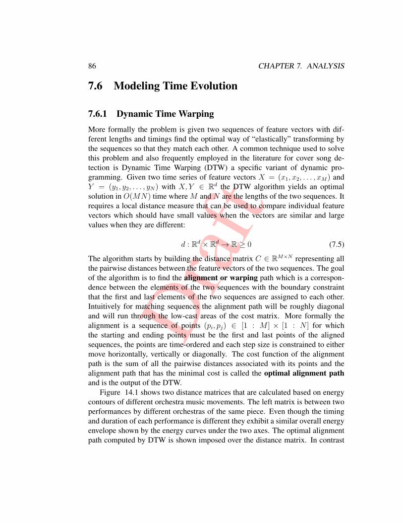
Dra
ft
86 CHAPTER 7. ANALYSIS
7.6 Modeling Time Evolution
7.6.1 Dynamic Time WarpingMore formally the problem is given two sequences of feature vectors with dif-ferent lengths and timings find the optimal way of “elastically” transforming bythe sequences so that they match each other. A common technique used to solvethis problem and also frequently employed in the literature for cover song de-tection is Dynamic Time Warping (DTW) a specific variant of dynamic pro-gramming. Given two time series of feature vectors X = (x1, x2, . . . , xM) andY = (y1, y2, . . . , yN) with X, Y ∈ Rd the DTW algorithm yields an optimalsolution in O(MN) time where M and N are the lengths of the two sequences. Itrequires a local distance measure that can be used to compare individual featurevectors which should have small values when the vectors are similar and largevalues when they are different:
d : Rd × Rd → R ≥ 0 (7.5)
The algorithm starts by building the distance matrix C ∈ RM×N representing allthe pairwise distances between the feature vectors of the two sequences. The goalof the algorithm is to find the alignment or warping path which is a correspon-dence between the elements of the two sequences with the boundary constraintthat the first and last elements of the two sequences are assigned to each other.Intuitively for matching sequences the alignment path will be roughly diagonaland will run through the low-cast areas of the cost matrix. More formally thealignment is a sequence of points (pi, pj) ∈ [1 : M ] × [1 : N ] for whichthe starting and ending points must be the first and last points of the alignedsequences, the points are time-ordered and each step size is constrained to eithermove horizontally, vertically or diagonally. The cost function of the alignmentpath is the sum of all the pairwise distances associated with its points and thealignment path that has the minimal cost is called the optimal alignment pathand is the output of the DTW.
Figure 14.1 shows two distance matrices that are calculated based on energycontours of different orchestra music movements. The left matrix is between twoperformances by different orchestras of the same piece. Even though the timingand duration of each performance is different they exhibit a similar overall energyenvelope shown by the energy curves under the two axes. The optimal alignmentpath computed by DTW is shown imposed over the distance matrix. In contrast
Dra
ft
7.7. FURTHER READING 87
(a) Good Alignment (b) Bad Alignment
Figure 7.1: Similarity Matrix between energy contours and alignment path using
Dynamic Time Warping
the matrix on the right shows the distance matrix between two unrelated orchestralmovements where it is clear there is no alignment.
7.6.2 Hidden Markov Models
7.6.3 Kalman and Particle Filtering
7.7 Further Readingcite Mitchell, Duda and Hart, Theodoridis and Bishop.

Dra
ft
88 CHAPTER 7. ANALYSIS
Dra
ftPart II
Tasks
89

Dra
ft
Dra
ftChapter 8
Similarity Retrieval
Similarity retrieval (or query-by-example) is one of the most fundamental MIRtasks. It is also one of the first tasks that were explored in the literature. Itwas originally inspired by ideas from text information retrieval and this earlyinfluence is reflected in the naming of the field. Today most people with computersuse search engines on a daily basis and are familiar with the basic idea of textinformation retrieval. The user submits a query consisting of some words to thesearch engine and the search engine returns a ranked list of web pages sorted byhow relevant they are to the query.
Similarity retrieval can be viewed as an analogous process where instead of theuser querying the system by providing text the query consists of an actual pieceof music. The system then responds by returning a list of music pieces ranked bytheir similarity to the query. Typically the input to the system consists of the querymusic piece (using either a symbolic or audio representation) as well as additionalmetadata information such as the name of the song, artist, year of release etc. Eachreturned item typically also contains the same types of meta-data. In addition tothe audio content and meta-data other types of user generated information canalso be considered such as ranking, purchase history, social relations and tags.Similarity retrieval can also be viewed as a basic form of playlist generation inwhich the returned results form a playlist that is “seeded” by the query. Howevermore complex scenarios of playlist generation can be envisioned. For example astart and end seed might be specified or additional constraints such as approximateduration or minimum tempo variation can be specified. Another variation is based
91
Dra
ft
92 CHAPTER 8. SIMILARITY RETRIEVAL
on what collection/database is used for retrieval. The term playlisting is morecommonly used to describe the scenario where the returned results come from thepersonal collection of the user, while the term recommendation is more commonlyused in the case where the returned results are from a store containing a largeuniverse of music. The purpose of the recommendation process is to entice theuser to purchase more music pieces and expand their collection. Although thesethree terms (similarity retrieval, music recommendation, automatic playlisting)have somewhat different connotations the underlying methodology for solvingthem is similar so for the most part we will use them interchangeably. Anotherrelated term that is sometimes used in personalized radio in which the idea is toplay music that is personalized to the preferences to the user.
One can distinguish three basic approaches to computing music similarity.Content-based similarity is performed by analyzing the actual content to extractthe necessary information. Metadata approaches exploit sources of informationthat are external to the actual content such as relationships between artists, styles,tags or even richer sources of information such as web reviews and lyrics. Usage-based approaches track how users listen and purchase music and utilize this in-formation for calculating similarity. Examples include collaborative filtering inwhich the commonalities between purchasing histories of different users are ex-ploited, tracking peer-to-peer downloads or radio play of music pieces to evaluatetheir “hotness” and utilizing user generated rankings and tags.
There are trade-offs involved in all these three approaches and most likelythe ideal system would be one that combines all of them intelligently. Usage-based approaches suffer from what has been termed the “cold-start” problem inwhich new music pieces for which there is no usage information can not be rec-ommended. Metadata approaches suffer from the fact that metadata information isfrequently noisy or inaccurate and can sometimes require significant semi-manualeffort to clean up. Finally content-based methods are not yet mature enough toextract high-level information about the music.
From a data mining perspective similarity retrieval can be considered a rankingproblem. Given a query music track q and a collection of music tracks D thegoal of similarity retrieval is to return a ranked list of the music tracks in Dsorted by similarity so that the most similar objects are at the top of the list.In most approaches this ranking is calculated by defining some similarity (ordistance) metric between pairs of music tracks. The most basic formulation isto represent each music track as a single feature vector of fixed dimensionalityx = [x1, x2, . . . , xn]T and use standard distance metrics such as L1 (Manhattan)or L2 (Euclidean) or Mahalanobis on the resulting high dimensional space. This
Dra
ft
93
feature vector is calculated using audio feature extraction techniques as describedin the following sections. Unless the distance metric is specifically designed tohandle features with different dynamic ranges the feature vectors are typicallynormalized for example by scaling all of them so that their maximum value overthe dataset is 1 and their minimum value is 0. A more complex alternative is totreat each music track as a distribution of feature vectors. This is accomplished byassuming that the feature vectors are samples of an unknown underlying prob-ability density function that needs to be estimated. By assuming a particularparametric form for the pdf (for example a Gaussian Mixture Model) the musictrack is then represented as a parameter vector θ that is estimated from the data.This way the problem of finding the similarity between music tracks is trans-formed to the problem of somehow finding the difference between two probabilitydistributions. Several such measures of probability distance have been proposedsuch as histogram intersection, symmetric Kullback-Leibler divergence and earthmover’s distance. In general computation of such probabilistic distances are morecomputationally intensive than geometric distances on feature vectors and in manycases require numerical approximation as they can not be obtained analytically.An alternative to audio feature extraction is to consider similarity based on textsuch as web pages, user tags, blogs, reviews, and song lyrics. The most commonmodel when dealing with text is the so called “bag of words” representation inwhich each document is represented as an unordered set of its words withouttaking into account any syntax or structure. Each word is assigned a weight thatindicates the importance of the word for some particular task. The document canthen be represented as a feature vector comprising of the weights correspondingto all the words of interest. From a data mining perspective the resulting featurevector is no different than the ones extracted from audio feature extraction andcan be handled using similar techniques. In the previous section we described aparticular example of text based feature extraction for the purpose of predictingthe country of origin as an artist.
As an example of how a text-based approach can be used to calculate similarityconsider the problem of finding how similar are two artists A and B. Each artistis characterized by a feature vector consisting of term weights for the terms theyhave in common. The cosine similarity between the two feature vectors is definedas the cosine of the angle between the vectors and has the property that it is notaffected by the magnitude of the vector (which would correspond to the absolutenumber of times terms appear and could be influenced by the popularity of theartist):
Dra
ft
94 CHAPTER 8. SIMILARITY RETRIEVAL
sim(A,B) = cosθ =
∑tA(t)×B(t)√∑
tA(t)2 ×√∑
tB(t)2(8.1)
Another approach to calculating similarity is to assume that the occurrenceof two music tracks or artists within the same context indicates some kind ofsimilarity. The context can be web pages (or page counts returned by a searchengine), playlists, purchase histories, and usage patterns in peer-to-peer (P2P)networks. Collaborative filtering (CF) refers to a set of techniques that makerecommendations to users based on preference information from many users. Themost common variant is to assume that the purchase history of a particular user (orto some extent equivalently their personal music collections) is characteristic oftheir taste in music. As an example of how co-occurrence can be used to calculatesimilarity, a search engine can be queries individually for documents that containa particular artist A and B, as well as documents that contain both A and B. Theartist similarity between A and B can then be found by:
sim(A,B) =co(A,B)
min(co(A), co(B))(8.2)
where co(X) is the number of pages returned for queryX or the co-occurrences ofA and B in some context. A similar measure can be defined based co-occurrencesbetween tracks and artists in playlists and compilation albums based on condi-tional probabilities:
sim(A,B) =1
2∗(co(A,B)
co(A)+co(A,B)
co(B)
)(8.3)
Co-occurrences can also be defined in the context of peer-to-peer networksby considering the number of users that have both artists A and B in their sharedcollection. The popularity bias refers to the problem of popular artists appearingmore similar than they should be due to them occurring in many contexts. Asimilarity measure can be designed to down weight the similarity between artistsif one of them is very popular and the other is not (the right-hand part of thefollowing equation):
sim(A,B) =C(A,B)
C(B)∗(
1− |C(A)− C(B)|C(Max)
)(8.4)
whereC(Max) is the number of times the most popular artist appears in a context.
Dra
ft
95
8.0.1 Evaluation of similarity retrieval
One of the challenges in content-based similarity retrieval is evaluation. In eval-uating mining systems ideally one can obtain ground truth information that isidentical to the outcome of the mining algorithm. Unfortunately this is not thecase in similarity as it would require manually sorting large collections of musicin order of similarity to a large number of queries. Even for small collections andnumber of queries collecting such data would be extremely time consuming andpractically impossible. Instead the more common approach is to only consider thetop K results for each query where K is a small number and have users annotateeach result as relevant or not relevant. Sometimes a numerical discrete score isused instead of a binary relevance decision. Another possibility that has beenused is to assume that tracks by the same artist or same genre should be similarand use such groupings to assign relevance values.
Evaluation metrics based on information retrieval can be used to evaluate theretrieved results for a particular query. They assume that each of the returnedresults has a binary annotation indicating whether or not it is relevant to the query.The most common one is the F-measure which is a combination of the simplermeasures of Precision and Recall. Precision is the fraction of retrieved instancesthat are relevant. Recall is the fraction of relevant instances that are retrieved. Asan example consider a music similarity search in which relevance is defined bygenre. If for a given query of Reggae music it returns 20 songs and 10 of them arealso Reggae the precision for that query is 10/20
=0.5. If there are a total of 30 reggae
songs in the collection searched then the Relevance for that query is 1030
= 0.33.The F-measure is defined as the harmonic mean of Precision P and Recall R.
F = 2× P ×RP +R
(8.5)
These three measures are based on the list of documents returned by the systemwithout taking into account the order they are returned. For similarity retrieval amore accurate measure is the Average Precision which is calculated by computingthe precision and recall at every position in the ranked sequence of documents,creating a precision-recall curve and computing the average. This is equivalent tothe following finite sum:
AP =
∑nk=1 P (k)× rel(k)
#relevantdocuments(8.6)

Dra
ft
96 CHAPTER 8. SIMILARITY RETRIEVAL
where P(k) is the precision at list position k and rel(k) is an indicator function thatis 1 if the item at list position (or rank) k is a relevant document and 0 otherwise.
All of the measures described above are defined for a single query. They caneasily be extended to multiple queries by taking their average across the queries.The most common way of evaluating similarity systems with binary relevanceground-truth is the Mean Average Precision (MAP) which the defined as the meanof the Average Precision across a set of queries.
The Music Information Retrieval Evaluation Exchange (MIREX) is an annualevaluation benchmark in which different groups submit algorithms to solve vari-ous MIR tasks and their performance is evaluated using a variety of subjective andobjective metrics. Table ?? shows representative results of the music similarityand retrieval task from 2010. It is based on a dataset of 7000 30-second audioclips drawn from 10 genres. The objective statistics are the precision at 5, 10, 20and 50 retrieved items without counting entries by the artist (artist filtering). Thesubjective statics are based on human evaluation of approximately 120 randomlyselected queries and 5 results per query. Each result is graded with a fine score(between 0 and 100 with 100 being most similar) and a broad score (0 not similar,1 somewhat similar, 2 similar) and the results are averaged. As can be seen allautomatic music similarity systems perform significantly better than the randombaseline (RND). The differ in terms of the type of extracted features utilized,the decision fusion strategy (such as simple concatenation of the different featuresets or empirical combinations of distances from the individual feature sets), andwhether post-processing is applied to the resulting similarity matrix. There isalso a strong correlation between the subjective and objective measures althoughit is not perfect (for example SSPK2 is better than PSS1 in terms of subjectivemeasures but worst in terms of objective measures).

Dra
ft
97
FS BS P@5 P@10 P@20 P@50
RND 17 0.2 8 9 9 9
TLN3 47 0.97 48 47 45 42
TLN2 47 0.97 48 47 45 42
TLN1 46 0.94 47 45 43 40
BWL1 50 1.08 53 51 50 47
PS1 55 1.22 59 57 55 51
PSS1 55 1.21 62 60 58 55
SSPK2 57 1.24 59 58 56 53
Table 8.1: 20120 MIREX Music Similarity and Retrieval Results

Dra
ft
98 CHAPTER 8. SIMILARITY RETRIEVAL
Dra
ftChapter 9
Classification
9.1 Classification
In the last 10 years musical genre classification of audio signals has been widelystudied and can be viewed as a canonical problem in which audio feature ex-traction has been used. Frequently new approaches to audio feature extractionare evaluated in the context of musical genre classification. They include sparseovercomplete representations [28] as well as bio-inspired joint acoustic and mod-ulation frequency represenations [78].
Audio classification has a long history in the area of Speech Recognition buthas only recently been applied to music. Even though there was some earlier work[58, 88] a good starting point for audio-based musical genre classification is thesystem that was proposed in 2002 by Tzanetakis [94].
Once the audio feature are extracted they need to be used to “train” a clas-sifier using supervised learning techniques. This is accomplished using all thelabeled audio feature representations for a training collection tracks. If the audiofeature representation has been summarized over the entire track to a single high-dimensional feature vector then this corresponds to the “classic” formulation ofclassification and any machine learning classifier can be used directly. Examplesof classifiers that have been used in the context of audio-based music classificationinclude: Gaussian Mixture Models [4, 94], Support Vector Machines [71, 62], andAdaBoost [10]. Another alternative is to perform classification in smaller seg-
99
Dra
ft
100 CHAPTER 9. CLASSIFICATION
ments and then aggregate the results using majority voting. A more complicatedapproach (frequently called bag-of-frames) consists of modeling each track usingdistribution estimation methods for example a Gaussian Mixture Model trainedusing the EM-algorithm. In this case each track is representanted as a probabilitydistribution rather than a single high-dimensional point (feature vector). Thedistance between the probability distributions can be estimated for example usingKL-divergence or approximations of it for example using the Monte-Carlo methoddepending on the particular parametric form used for density estimation. Byestablishing a distance metric between tracks it is possible to perform retrievaland classification by simple techniques such as k-nearest neighbors [4].
Evaluation of classification is relatively straightforward and in most waysidentical to any classification task. The standard approach is to compare thepredicted labels with ground truth labels. Common metrics include classificationaccuracy as well as retrieval metrics such as precision, recall, f-measure. When re-trieval metrics are used it is assumed that for a particular query revelant documentsare the tracks with the same genre label. Cross-validation is a technique frequentlyused in evaluating classification where the labeled data is split into training andtesting sets in different ways to ensure that the metrics are not influenced bythe particular choice of training and testing data. One detail that needs to betaken into account is the so-called album effect in which classification accuracyimproves when tracks from the same album are included in both training andtesting data. The cause is recording production effects that are common betweentracks in the same album. The typical approach is to ensure that when performingcross-validation tracks from the same album or artist only go to either the trainingor testing dataset.
Classification accuracy on the same dataset and using the same cross-validationapproach can be used for comparing the relative performance of different algo-rithms and design choices. Interpreting the classification accuracy in absoluteterms is trickier because of the subjective nature of genre labeling as has alreadybeen discussed in the section on ground truth labeling. In the early years ofresearch in audio-based musical genre classification each research group utilizeddifferent datasets, cross-validation approaches and metrics making it hard to drawany conclusions about the merits of different approaches. Sharing datasets isharder due to copyright restrictions. The Music Information Retrieval EvaluationExchange (MIREX) [25] is an annual event where different MIR algorithms areevaluated using a variety of metrics on different tasks including several audio-based classification tasks. The participants submit their algorithms and do nothave access to the data which addresses both the copy-right problem and the issue

Dra
ft
9.2. EMOTION/MOOD 101
Genre Classification 66.41
Genre Classification (Latin) 65.17
Audio Mood Classification 58.2
Artist Identification 47.65
Classical Composer Identification 53.25
Audio Tag Classification 0.28
Table 9.1: Audio-based classification tasks for music signals (MIREX 2009)
of over-fitting to a particular dataset. Table 9.1 shows representative results ofof the best performing system in different audio classification tasks from MIREX2009. With the exception of Audio Tag Classification all the results are percent-ages of classification accuracy. For audio tag classification the average f-measureis used instead.
9.2 Emotion/Mood
9.3 Instrument
[45]
9.4 Other
music/speech

Dra
ft
102 CHAPTER 9. CLASSIFICATION
9.5 Symbolic[53]
9.6 Further Reading[92]

Dra
ftChapter 10
Structure
[32]
10.1 Segmentation[49]
10.2 Alignment[?] [?]
10.3 Structure Analysis
103

Dra
ft
104 CHAPTER 10. STRUCTURE

Dra
ftChapter 11
Transcription
11.1 Monophonic Pitch Tracking[9], [54]
11.2 Transcription[8]
11.3 Chord Detection[6]
105

Dra
ft
106 CHAPTER 11. TRANSCRIPTION

Dra
ftChapter 12
Symbolic Representations
Music throughout most of human history was trasmitted orally and only existedephemerally at the time and place it was performed. Language and poetry weresimilarly orally transmitted until the development of writing which allowed lin-guistic information to be preserved over time and space using physical objectssuch as clay tablets. Cuniform script is one of the earliest forms of writing and itis perhaps not surprising that one of the earliest examples of music notation is incuniform dated to 2000 BC.
Over time several cultures developed a variety of music notation systems. Tosome extent all these notation systems can be considered as mnemonic aids forperformers differing in the type of information they encode.
[18][19]
107

Dra
ft
108 CHAPTER 12. SYMBOLIC REPRESENTATIONS
Dra
ftChapter 13
Queries
13.1 Query by example
13.2 Query by humming[73] [11] [76]
109

Dra
ft
110 CHAPTER 13. QUERIES

Dra
ftChapter 14
Fingerprinting and Cover Song
Detection
14.1 Fingerprinting
[2] [44]
14.2 Cover song detection
In addition to content-based similarity there are two related music mining prob-lems. The goal of audio fingerprinting is to identify whether a music track is oneof the recordings in a set of reference tracks. The problem is trivial if the twofiles are byte identical but can be considerably more challenging when varioustypes of distortion need to be taken into account. The most common distortion isperceptual audio compression (such as mp3 files) which can result in significantalterations to the signal spectrum. Although these alterations are not directlyperceptible by humans they make the task of computer identification harder. An-other common application scenario is music matching/audio fingerprinting formobile applications in which the query signal is acquired through a low quality
111

Dra
ft
112 CHAPTER 14. FINGERPRINTING AND COVER SONG DETECTION
microphone on a mobile phone and contains significant amount of backgroundnoise and interference. At the same time the underlying signal is the same exactmusic recording which can help find landmark features and representations thatare invariant to these distortions. Cover song detection is the more subtle problemof finding versions of the same song possibly performed by different artists, instru-mentation, tempo. As the underlying signals are completely different it requiresthe use of more high level representations such as chroma vectors that captureinformation about the chords and the melody of the song without being affectedby timbral information. In addition it requires sophisticated sequence matchingapproaches such as dynamic time warping (DTW) or Hidden Markov Models(HMM) to deal with the potential variations in tempo. Although both of theseproblems can be viewed as content-based similarity retrieval problems with anappropriately defined notion of similarity they have some unique characteristics.Unlike the more classic similarity retrieval in which we expect the returned resultsto gradually become less similar, in audio fingerprinting and cover song detectionthere is a sharper cutoff defining what is correct or not. In the ideal case copiesor cover versions of the same song should receive a very high similarity scoreand everything else a very low similarity score. This specificity is the reason whytypically approaches that take into account the temporal evolution of features aremore common.
Audio fingerprinting is a mature field with several systems being actively usedin industry. As a representative example we describe a landmark-based audiofingerprinting system based on the ideas used by Shazam which is a music match-ing service for mobile phones. In this scheme each audio track is representedby the location in time and frequency of prominent peaks of the spectrogram.Even though the actual amplitude of these peaks might vary due to noise andaudio compression their actual location in the time frequency plane is preservedquite well in the presence of noise and distortion. The landmarks are combinedinto pairs and each pair is characterized by three numbers f1, f2, t which are thefrequency of the first peak, the frequency of the second peak and the time betweenthem. Both reference tracks and the query track are converted into this landmarkrepresentation. The triplets characterizing each pair are quantized with the basicidea being that if the query and a reference track have a common landmarkswith consistent timing they are a match. The main challenge in an industrialstrength implementation is deciding on the number of landmarks per second andthe thresholds used for matching. The lookup of the query landmarks into thelarge pool of reference landmarks can be performed very efficiently using hashing

Dra
ft
14.2. COVER SONG DETECTION 113
techniques to effectively create an inverted index which maps landmarks to thefiles they originate.
To solve the audio cover song detection problem there are two issues thatneed to be addressed. The first issue is to compute a representation of the audiosignal that is not affected significantly by the timbre of the instruments playingbut still captures information about the melody and harmony (the combination ofdiscrete pitches that are simultaneously sounding) of the song. The most commonrepresentation used in music mining for this purpose are chroma vectors (or pitchclass profiles) which can be thought of as histograms showing the distributionof energy among different discrete pitches. The second issue that needs to beaddressed is how to match two sequence of feature vectors (chroma vectors inthis case) that have different timing and length as there is no guarantee that acover song is played at the same tempo as the original and there might be multiplesections with different timing each.
More formally the problem is given two sequences of feature vectors withdifferent lengths and timings find the optimal way of “elastically” transformingby the sequences so that they match each other. A common technique usedto solve this problem and also frequently employed in the literature for coversong detection is Dynamic Time Warping (DTW) a specific variant of dynamicprogramming. Given two time series of feature vectors X = (x1, x2, . . . , xM)and Y = (y1, y2, . . . , yN) with X, Y ∈ Rd the DTW algorithm yields an optimalsolution in O(MN) time where M and N are the lengths of the two sequences. Itrequires a local distance measure that can be used to compare individual featurevectors which should have small values when the vectors are similar and largevalues when they are different:
d : Rd × Rd → R ≥ 0 (14.1)
The algorithm starts by building the distance matrix C ∈ RM×N representing allthe pairwise distances between the feature vectors of the two sequences. The goalof the algorithm is to find the alignment or warping path which is a correspon-dence between the elements of the two sequences with the boundary constraintthat the first and last elements of the two sequences are assigned to each other.Intuitively for matching sequences the alignment path will be roughly diagonaland will run through the low-cast areas of the cost matrix. More formally thealignment is a sequence of points (pi, pj) ∈ [1 : M ] × [1 : N ] for whichthe starting and ending points must be the first and last points of the alignedsequences, the points are time-ordered and each step size is constrained to either

Dra
ft
114 CHAPTER 14. FINGERPRINTING AND COVER SONG DETECTION
move horizontally, vertically or diagonally. The cost function of the alignmentpath is the sum of all the pairwise distances associated with its points and thealignment path that has the minimal cost is called the optimal alignment pathand is the output of the DTW.
(a) Good Alignment (b) Bad Alignment
Figure 14.1: Similarity Matrix between energy contours and alignment path using
Dynamic Time Warping
Figure 14.1 shows two distance matrices that are calculated based on energycontours of different orchestra music movements. The left matrix is between twoperformances by different orchestras of the same piece. Even though the timingand duration of each performance is different they exhibit a similar overall energyenvelope shown by the energy curves under the two axes. The optimal alignmentpath computed by DTW is shown imposed over the distance matrix. In contrastthe matrix on the right shows the distance matrix between two unrelated orchestralmovements where it is clear there is no alignment.
Cover song detection is performed by applying DTW between all the querysong and all the references and returning as a potential match the one with theminimum total cost for the optimal alignment path. Typically the alignment costbetween covers of the same song will be significantly lower than the alignmentcost between two random songs. DTW is a relatively costly operation and there-fore this approach does not scale to large number of songs. A common solutionfor large scale matching is to apply an audio fingerprinting type of approach withefficient matching to filter out a lot of irrelevant candidates and once a sufficientsmall number of candidate reference tracks have been selected apply pair-wiseDTW between the query and all of them.

Dra
ft
14.2. COVER SONG DETECTION 115
RE SZA TA
Mean # of covers in top 10 6.20 7.35 1.96
Mean Average Precision 0.66 0.75 0.20
Mean Rank of first correct cover 2.28 6.15 29.90
Table 14.1: 2009 MIREX Audio Cover Song Detection - Mixed Collection
RE SZA TA
Mean # of covers in top 10 8.83 9.58 5.27
Mean Average Precision 0.91 0.96 0.56
Mean Rank of first correct cover 1.68 1.61 5.49
Table 14.2: 2009 MIREX Audio Cover Song Detection - Mazurkas
Table 14.1 shows the results of the audio cover song detection task of MIREX2009 in the so called “mixed” collection which consists of 1000 pieces that contain11 “cover song” each represented by 11 different versions. As can be seen theperformance is far from perfect but it is still impressive given the difficulty of theproblem. An interesting observation is that the objective evaluation measures arenot consistent. For example the RE algorithm performs slightly worse than theSZA in terms of mean average precision but has been mean rank for the firstcorrectly identified cover. Table 14.2 shows the results of the MIREX 2009audio cover song detection task for the Mazurkas collection which consists 11different performances/versions of 49 Chopin Mazurkas. As can be seen fromthe results this is a easier dataset to find covers probably due to the smaller sizeand more uniformity in timbre. The RE algorithm is based on the calculation ofdifferent variants of chroma vectors utilizing multiple feature sets. In contrast tothe more common approach of scoring the references in a ranked list and settingup a threshold for identifying covers it follows a classification approach in whicha pair is either classified as reference/cover or as reference/non-cover. The SZAalgorithm is based on harmonic pitch class profiles (HPCP) which are similar
Dra
ft
116 CHAPTER 14. FINGERPRINTING AND COVER SONG DETECTION
to chroma vectors but computed over a sparse harmonic representation of theaudio signal. The sequence of feature vectors of one song is transposed to themain tonality of the other song in consideration. A state space representation ofembedding m and time delay z is used to represent the time series of HPCP witha recurrence quantification measure used for calculating cover song similarity.

Dra
ftChapter 15
Other topics
In this chapter we cover several MIR topics that either are emerging or theirassociated literature is limited or both.
15.1 Optical Music Recognition
[16] [70] [?]
15.2 Digital Libraries and Metadata
[5], [26] [?], [66] [27]
15.3 Computational Musicology
15.3.1 Notated Music
[17] [57]
117
Dra
ft
118 CHAPTER 15. OTHER TOPICS
15.3.2 Computational Ethnomusicology[35] [13] [?] [?] [?] [?]
15.3.3 MIR in live music performance
15.4 Further Reading
Dra
ftPart III
Systems and Applications
119

Dra
ft

Dra
ftChapter 16
Interaction
16.1 Interaction[36]
[?]
121

Dra
ft
122 CHAPTER 16. INTERACTION

Dra
ftChapter 17
Evaluation
17.1 Bibliography
123

Dra
ft
124 CHAPTER 17. EVALUATION

Dra
ftChapter 18
User Studies
[?] [?] [?]
125

Dra
ft
126 CHAPTER 18. USER STUDIES
Dra
ftChapter 19
Tools
Although frequently researchers implement their own audio feature extractionalgorithms there are several software collections that are freely available thatcontain many of the methods described in this chapter. They have enabled re-searchers more interested in the data mining and machine learning aspects ofmusic analysis to build systems more easily. They differ in the programminglanguage/environment they are written, the computational efficiency of the ex-traction process, their ability to deal with batch processing of large collections,their facilities for visualizing feature data, and their expressiveness/flexibility indescribing complex algorithms.
Table 19.1 summarizes information about some of the most commonly usedsoftware resources as of the year 2010. The list is by no means exhaustive butdoes provide reasonable coverage of what is available. Several of the figures inthis chapter were created using Marsyas and some using custom MATLAB code.
19.1 Datasets
[38]
127
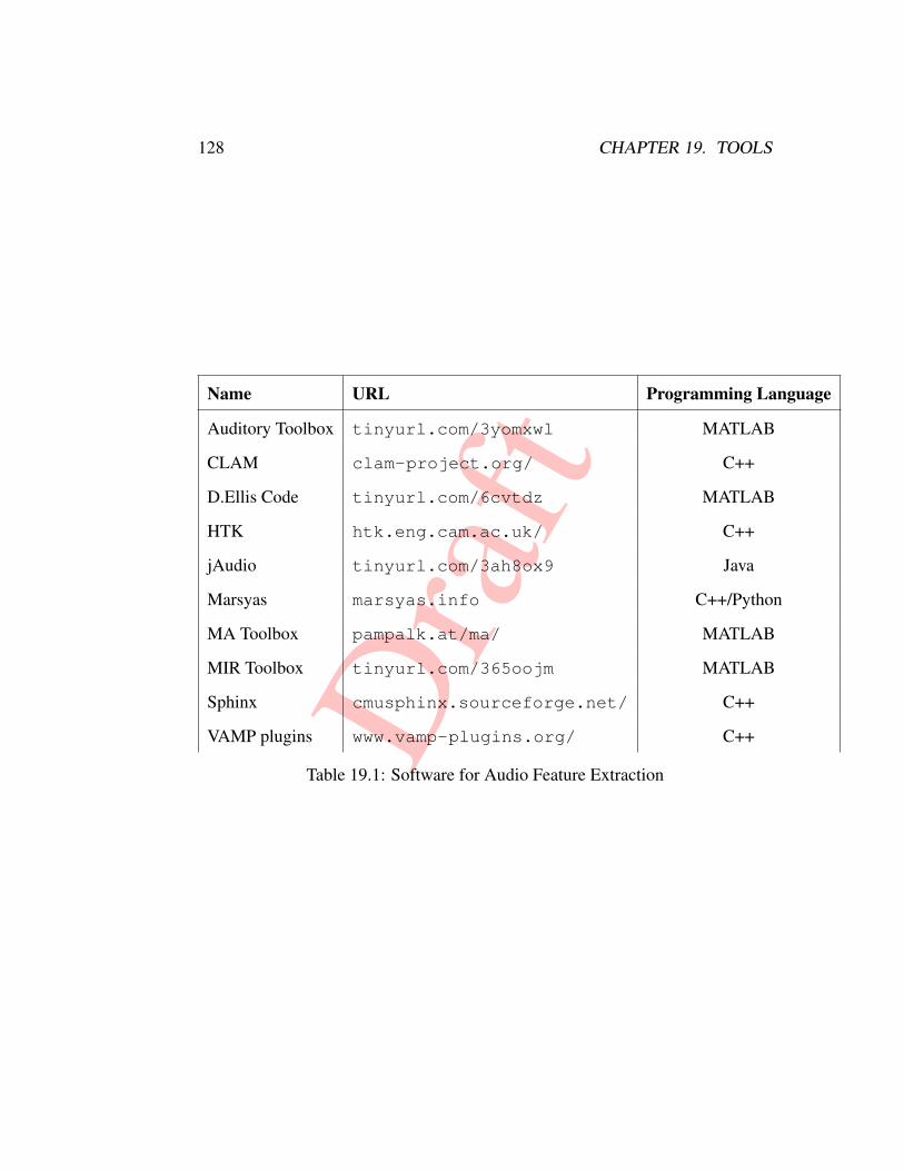
Dra
ft
128 CHAPTER 19. TOOLS
Name URL Programming Language
Auditory Toolbox tinyurl.com/3yomxwl MATLAB
CLAM clam-project.org/ C++
D.Ellis Code tinyurl.com/6cvtdz MATLAB
HTK htk.eng.cam.ac.uk/ C++
jAudio tinyurl.com/3ah8ox9 Java
Marsyas marsyas.info C++/Python
MA Toolbox pampalk.at/ma/ MATLAB
MIR Toolbox tinyurl.com/365oojm MATLAB
Sphinx cmusphinx.sourceforge.net/ C++
VAMP plugins www.vamp-plugins.org/ C++
Table 19.1: Software for Audio Feature Extraction

Dra
ft
19.2. DIGITAL MUSIC LIBRARIES 129
19.2 Digital Music LibrariesVARIATIONS

Dra
ft
130 CHAPTER 19. TOOLS

Dra
ftAppendix A
Statistics and Probability
A brief overview of the necessary concepts.Email Ashley to send me his PhD thesis
131

Dra
ft
132 APPENDIX A. STATISTICS AND PROBABILITY
Dra
ftAppendix B
Project ideas
In this Appendix some project ideas related to music information retrieval areprovided. They have been used in the Music Information Retrieval course taughtat the University of Victoria and are appropriate for class projects with small teams(2-3 students).
133

Dra
ft
134 APPENDIX B. PROJECT IDEAS
Dra
ftAppendix C
Commercial activity 2011
Commercial activity in MIR related topics is in constant flux so it is hard toprovide comprehensive information about it. At the same time it is interesting toobserve which algorithms and techniques described in this book are actively usedin real world applications. This appendix attempts to provide a snapshot of thecurrent state of commercial activity in 202. The list of companies and systemsdescribed is by no means exhaustive but tries to be representative of existingactivity.
135

Dra
ft
136 APPENDIX C. COMMERCIAL ACTIVITY 2011

Dra
ftAppendix D
Historic Time Line
In this Appendix I provide a list of historic milestones both academic and com-mercial in the emerging field of Music Information Retrieval. As is the case withany such attempt the resulting list is to some extent idiosyncratic. My hope is thatit provides a picture of how the field evolved over time and helps readers situatethe techniques and developments described in this book in time.
137

Dra
ft
138 APPENDIX D. HISTORIC TIME LINE

Dra
ftBibliography
[1] E. Allamanche, J. Herre, O. Hellmuth, B. Froba, and T. Kastner. Content-based identification of audio material using MPEG-7 low level description.In Int. Conf. on Music Information Retrieval (ISMIR), 2001.
[2] E. Allamanche, J. Herre, O. Hellmuth, B. Froba, T. Kastner, and M. Cremer.Content-based identification of audio material using mpeg-7 low leveldescription. In Proceedings of the International Conference on MusicInformation Retrieval (ISMIR), 2001.
[3] J. J. Aucouturier and F. Pachet. Music similarity measures: What’s the use ?In Int. Conf. on Music Information Retrieval (ISMIR), 2002.
[4] J. J. Aucouturier and F. Pachet. Representing musical genre: A state of theart. Journal of New Music Research, 32(1):1–2, 2003.
[5] D. Bainbridge. The role of music ir in the new zealand digital musiclibrary project. In Proceedings of the International Conference on MusicInformation Retrieval (ISMIR), 2000.
[6] J. Barthelemy. Figured bass and tonality recognition. In Proceedings of theInternational Conference on Music Information Retrieval (ISMIR), 2001.
[7] M. A. Bartsch and G. H. Wakefield. To catch a chorus: using chroma-based represenations for audio thumbnailing. In Workshop on Applicationsof Signal Processing to Audio and Acoustics, pages 150–18, 2001.
[8] J. P. Bello, G. Monti, and M. Sandler. Techniques for automatic musictranscription. In Proceedings of the International Conference on MusicInformation Retrieval (ISMIR), 2000.
139
Dra
ft
140 BIBLIOGRAPHY
[9] D. Bendor and M. Sandler. Time domain extraction of vibrato frommonophonic instruments. In Proceedings of the International Conferenceon Music Information Retrieval (ISMIR), 2000.
[10] J. Bergstra, N. Casagrande, D. Erhan, D. Eck, and B. Kegl. Aggregatefeatures and AdaBoost for music classification. Machine Learning, 65(2-3):473–484, 2006.
[11] W. P. Birmingham, R. B. Dannenberg, G. H. Wakefield, M. A. Bartsch,D. Mazzoni, C. Meek, M. Mellody, and W. Rand. Musart: Music retrievalvia aural queries. In Proceedings of the International Conference on MusicInformation Retrieval (ISMIR), 2001.
[12] P. Boersma. Accurate short-term analysis of the fundamental frequency andthe harmonics-to-noise ratio of a sampled sound. Proceedings of the Instituteof Phonetic Sciences, 17:97–110, 1993.
[13] A. Bonardi. Ir for contemporary music: What the musicologist needs. InProceedings of the International Conference on Music Information Retrieval(ISMIR), 2000.
[14] A. Bregman. Auditory Scene Analysis. MIT Press, Cambridge, 1990.
[15] M. Casey. Sound classification and similarity tools. In B. Manjunath,P. Salembier, and T. Sikora, editors, Introduction to MPEG-7: MultimediaContent Description Language, pages 309–323. J. Wiley, 2002.
[16] G. S. Choudhury, T. DiLauro, M. Droettboom, I. Fujinaga, B. Harrington,and K. MacMillan. Optical music recognition system within a large-scaledigitization project. In Proceedings of the International Conference onMusic Information Retrieval (ISMIR), 2000.
[17] M. Clausen, R. Engelbrecht, D. Meyer, and J. Schmitz. Proms: A web-basedtool for searching in polyphonic music. In Proceedings of the InternationalConference on Music Information Retrieval (ISMIR), 2000.
[18] D. Cliff and H. Freeburn. Exploration of point-distribution models forsimilarity-based classification and indexing of polyphonic music. InProceedings of the International Conference on Music Information Retrieval(ISMIR), 2000.

Dra
ft
BIBLIOGRAPHY 141
[19] M. Crochemore, C. S. Iliopoulos, Y. J. Pinzon, and W. Rytter. Findingmotifs with gaps. In Proceedings of the International Conference on MusicInformation Retrieval (ISMIR), 2000.
[20] R. Dannenberg and N. Hu. Pattern discovery techniques for music audio.Journal of New Music Research, June 2003:153–164, 2003.
[21] I. Daubechies. Orthonormal bases of compactly supported wavelets.Communications on Pure and Applied Math, 41:909–996, 1988.
[22] S. Davis and P. Mermelstein. Experiments in syllable-based recognition ofcontinuous speech. IEEE Transcactions on Acoustics, Speech and SignalProcessing, 28:357–366, Aug. 1980.
[23] A. de Cheveigne and H. Kawahara. YIN, a fundamental frequencyestimator for speech and music. Journal of Acoustical Society of America,111(4):1917–1930, 2002.
[24] S. Dixon. Onset detection revisited. In Int. Conf. on Digital Audio Effects(DAFx), 2006.
[25] J. S. Downie. The music information retrieval evaluation exchange (2005-2007): A window into music information retrieval. Acoustical Science andTechnology, 29(4):247–255, 2008.
[26] J. W. Dunn. Beyond variations: Creating a digital music library. InProceedings of the International Conference on Music Information Retrieval(ISMIR), 2000.
[27] J. W. Dunn, M. W. Davidson, and E. J. Isaacson. Indiana university digitalmusic library project: An update. In Proceedings of the InternationalConference on Music Information Retrieval (ISMIR), 2001.
[28] L. D. E. Ravelli, G. Richard. Audio signal representations for indexingin the transform domain. IEEE Trans. on Audio, Speech, and LanguageProcessing, 18(3):434–446, 2010.
[29] D. Ellis and G. H. Poliner. Identifying cover songs with chroma features anddynamic programming beat tracking. In Int. Conf. on Acoustics, Speech, andSignal Processing (ICASSP), pages IV–1429–IV–1432, 2007.
Dra
ft
142 BIBLIOGRAPHY
[30] M. T. F. Morchen, A. Ultsch and I. Lohken. Modeling timbre distance withtemporal statistics from polyphonic music. IEEE Transactions on Audio,Speech and Language Processing, 8(1):81–90, 2006.
[31] J. Foote. Visualizing music and audio using self-similarity. In ACMMultimedia, pages 77–80, 1999.
[32] J. Foote. Arthur: Retrieving orchestral music by long-term structure. InProceedings of the International Conference on Music Information Retrieval(ISMIR), 2000.
[33] J. Foote, M. Cooper, and U. Nam. Audio retrieval by rhythmic similarity. InInt. Conf. on Music Information Retrieval (ISMIR), 2002.
[34] H. Fujihara, M. Goto, T. Kitahara, and H. G. Okuno. A modeling ofsinging voice robust to accompaniment sounds and its application to singeridentification and vocal-timbre similarity based music information retrieval.IEEE Trans. on Audio, Speech and Language Processing, 18(3):638–648,2010.
[35] G. Geekie. Carnatic ragas as music information retrieval entities. InProceedings of the International Conference on Music Information Retrieval(ISMIR), 2002.
[36] A. Georgaki, S. Raptis, and S. Bakamidis. A music interface for visuallyimpaired people in the wedelmusic environment. design and architecture. InProceedings of the International Conference on Music Information Retrieval(ISMIR), 2000.
[37] M. Good. Representing music using xml. In Proceedings of the InternationalConference on Music Information Retrieval (ISMIR), 2000.
[38] H. . N. T. . O. R. Goto, Masataka ; Hashiguchi. Rwc music database:Popular, classical and jazz music databases. In Proceedings of theInternational Conference on Music Information Retrieval (ISMIR), 2002.
[39] F. Gouyon, S. Dixon, E. Pampalk, and G. Widmer. Evaluating rhythmicdescriptors for musical genre classification. In AES 25th Int. Conf. onMetadata for Audio, pages 196–204, 2002.
Dra
ft
BIBLIOGRAPHY 143
[40] F. Gouyon, A. Klapuri, S. Dixon, M. Alonso, G. Tzanetakis, C. Uhle, andP. Cano. An experimental comparison of audio tempo induction algorithms.IEEE Trans. on Audio, Speech and Language Processing, 14(5):1832–1844,2006.
[41] J. Grey. Multidimensional perceptual scaling of musical timbres. Journal ofthe Acoustical Society of America, 61(5):1270–1277, 1977.
[42] M. Gruhne, C. Dittmar, and D. Gaertner. Improving rhythmic similaritycomputation by beat histogram transformations. In Int. Conf. on MusicInformation Retrieval, 2009.
[43] S. Hainsworth. Beat tracking and musical metre analysis. In A. Klapuri andM. Davy, editors, Signal Processing Methods for Music Transcription, pages101–129. Springer, New York, 2006.
[44] T. Haitsma, Jaap ; Kalker. A highly robust audio fingerprinting system. InProceedings of the International Conference on Music Information Retrieval(ISMIR), 2002.
[45] P. Herrera-Boyer, X. Amatriain, E. Batlle, and X. Serra. Towards instrumentsegmentation for music content description:a critical review of instrumentclassification techniques. In Proceedings of the International Conference onMusic Information Retrieval (ISMIR), 2000.
[46] A. Holzapfel and Y. Stylianou. Rhythmic similarity of music based ondynamic periodicity warping. In IEEE Int. Conf. on Acoustics, Speech andSignal Processing (ICASSP), pages 2217–2220, 2008.
[47] A. Holzapfel and Y. Stylianou. A scale transform based method for rhythmicsimilarity of music. In IEEE Int. Conf. on Acoustics, Speech and SignalProcessing (ICASSP), pages 317–320, 2009.
[48] H. H. Hoos, K. Renz, and M. Gorg. Guido/mir an experimental musicalinformation retrieval system based on guido music notation. In Proceedingsof the International Conference on Music Information Retrieval (ISMIR),2001.
[49] O. Izmirli. Using a spectral flatness based feature for audio segmentationand retrieval. In Proceedings of the International Conference on MusicInformation Retrieval (ISMIR), 2000.
Dra
ft
144 BIBLIOGRAPHY
[50] J. Jensen, M. Christensen, and S. Jensen. A tempo-insensitive representationof rhythmic patterns. In European Signal Processing Conference(EUSIPCO), 2009.
[51] J. H. Jensen, D. Ellis, M. Christensen, and S. H. Jensen. Evaluation ofdistance measures between gaussian mixture models of mfccs. In Int. Conf.on Music Information Retrieval (ISMIR), 2007.
[52] D. Jiang, L. Lu, H. Zhang, and J. Tao. Music type classification by spectralcontrast feature. In Int. Conf. on Multimedia and Expo (ICME), 2002.
[53] F. J. Kiernan. Score-based style recognition using artificial neural networks.In Proceedings of the International Conference on Music InformationRetrieval (ISMIR), 2000.
[54] Y. E. Kim, W. Chai, R. Garcia, and B. Vercoe. Analysis of a contour-basedrepresentation for melody. In Proceedings of the International Conferenceon Music Information Retrieval (ISMIR), 2000.
[55] Y. E. Kim and B. Whitman. Singer identification in popular music recordingsusing voice coding features. In Int. Conf. on Music Information Retrieval(ISMIR), 2002.
[56] T. Kitahara, Y. Tsuchihashi, and H. Katayose. Music genre classificationand similarity calculation using bass-line features. In Multimedia, 2008.ISM 2008. Tenth IEEE International Symposium on, 2008.
[57] A. Kornstadt. The jring system for computer-assisted musicologicalanalysis. In Proceedings of the International Conference on MusicInformation Retrieval (ISMIR), 2001.
[58] T. Lambrou, P. Kudumakis, R. Speller, M. Sandler, and A. Linnery.Classification of audio signals using statistical features on time and wavelettransform domains. In Int. Conf. on Acoustics, Speech and Signal Processing(ICASSP), 1998.
[59] C. Lee, J. L. Shih, K. Yu, and H. Lin. Automatic music genre classificationbased on modulation spectral analysis of spectral and cepstral features. IEEETrans. on Multimedia, 11(4):670–682, 2009.
Dra
ft
BIBLIOGRAPHY 145
[60] J. S. . R. A. Lee, Jin Ha ; Downie. Representing traditional korean musicnotation in xml. In Proceedings of the International Conference on MusicInformation Retrieval (ISMIR), 2002.
[61] K. Lee and M. Slaney. Acoustic chord transcription and key extraction fromaudio using key-dependent hmms trained on synthesized audio. IEEE Trans.on Audio, Speech and Language Processing, 16(2):291–301, 2008.
[62] T. Li and M. Ogihara. Detecting emotion in music. In Int. Symposium onMusic Information Retrieval (ISMIR), pages 239–240, 2003.
[63] T. Li and M. Ogihara. Toward intelligent music information retrieval. IEEETrans. on Multimedia, 8(3):564–574, 2006.
[64] T. Li and G. Tzanetakis. Factors in automatic musical genre classification. InProc. Workshop on applications of signal processing to audio and acousticsWASPAA, New Paltz, NY, 2003. IEEE.
[65] C. Liem and A. Hanjalic. Cover song retrieval: a comparative study ofsystem component choices. In Int. Conf. on Music Information Retrieval(ISMIR), 2009.
[66] K. Lin and T. Bell. Integrating paper and digital music information systems.In Proceedings of the International Conference on Music InformationRetrieval (ISMIR), 2000.
[67] A. Lindsay and Y. E. Kim. Adventures in standardization, or, how we learnedto stop worrying and love mpeg-7. In Proceedings of the InternationalConference on Music Information Retrieval (ISMIR), 2001.
[68] B. Logan. Mel frequency cepstral coefficients for music modeling. InProceedings of the International Conference on Music Information Retrieval(ISMIR), 2000.
[69] L. Lu, D. Lie, and H.-J. Zhang. Automatic mood detection and tracking ofmusic audio signals. IEEE Trans. on Speech and Audio Processing, 14(1):5–18, 2006.
[70] K. MacMillan, M. Droettboom, and I. Fujinaga. Gamera: A structureddocument recognition application development environment. In Proceedingsof the International Conference on Music Information Retrieval (ISMIR),2001.
Dra
ft
146 BIBLIOGRAPHY
[71] M. Mandel and D. Ellis. Song-level features and svms for musicclassification. In Int. Conf. on Music Information Retrieval (ISMIR), 2005.
[72] M. F. McKinney and J. Breebaart. Features for audio and musicclassification. In Int. Conf. on Music Information Retrieval (ISMIR), 2003.
[73] C. Meek and W. P. Birmingham. Thematic extractor. In Proceedings of theInternational Conference on Music Information Retrieval (ISMIR), 2001.
[74] A. Meng, P. Ahrendt, and J. Larsen. Temporal feature integration for musicgenre classification. IEEE Transactions on Audio, Speech and LanguageProcessing, 5(15):1654–1664, 2007.
[75] G. T. N. Hu, R. B. Dannenberg. Polyphonic audio matching and alignmentfor music retrieval. In Workshop on Applications of Signal Processing toAudio and Acoustics, 2003.
[76] T. Nishimura, H. Hashiguchi, J. Takita, J. X. Zhang, M. Goto, and R. Oka.Music signal spotting retrieval by a humming query using start framefeature dependent continuous dynamic programming. In Proceedings of theInternational Conference on Music Information Retrieval (ISMIR), 2001.
[77] T. Painer and A. Spanias. Perceptual coding of digital audio. Proceedings ofthe IEEE, 88(4):451–515, 2000.
[78] Y. Panagakis, C. Kotropoulos, and G. C. Arce. Non-negative multilinearprincipal component analysis of auditory temporal modulations for musicgenre classification. IEEE Trans. on Audio, Speech and LanguageProcessing, 18(3):576–588, 2010.
[79] J. Paulus and A. Klapuri. measuring the similarity of rhythmic patterns. InInt. Conf. on Music Information Retrieval (ISMIR), 2002.
[80] G. Peeters. Spectral and temporal periodicity representations of rhythm forthe automatic classification of music audio signal. IEEE Trans. on Audio,Speech, and Language Processing, (to appear), 2010.
[81] G. Peeters, A. L. Burthe, and X. Rodet. Toward automatic music audiosummary generation from signal analysis. In Int. Conf. on Music InformationRetrieval (ISMIR), 2002.

Dra
ft
BIBLIOGRAPHY 147
[82] D. Pye. Content-based methods for management of digital music. In Int.Conf. on Acoustics, Speech and Signal Processing (ICASSP), 2000.
[83] A. Rauber, E. Pampalk, and D. Merkl. The SOM-enhanced JukeBox:Organization and visualization of music collections based on perceptualmodels. Journal of New Music Research, 32(2):193–210, 2003.
[84] P. Roland. Xml4mir: Extensible markup language for music informationretrieval. In Proceedings of the International Conference on MusicInformation Retrieval (ISMIR), 2000.
[85] B. D. S. Essid, G. Richard. Musical instrument recognition by pairwiseclassification. IEEE Trans. on Audio, Speech and Language Processing,14(4):1401–1412, 2006.
[86] J. Serr and E. Gmez. Audio cover song identification based on tonalsequence alignment. In IEEE International Conference on Acoustics, Speechand Signal processing (ICASSP), pages 61–64, 2008.
[87] A. Sheh and D. P. W. Ellis. Chord segmentation and recognition using em-trained hidden markov models. In Int. Conf. on Music Information Retrieval(ISMIR), 2003.
[88] H. Sotlau, T. Schultz, M. Westphal, and A. Waibel. Recognition of musictypes. In Int. Conf. on Acoustics, Speech and Signal Processing (ICASSP),1998.
[89] E. Tsunoo. Audio genre classification using percussive pattern clusteringcombined with timbral features. In Int. Conf. on Multimedia and Expo(ICME), 2009.
[90] E. Tsunoo, N. Ono, and S. Sagayama. Musical bass-line pattern clusteringand its application to audio genre classification. In Int. Conf. on MusicInformation Retrieval (ISMIR), 2009.
[91] G. Tzanetakis and P. Cook. Multi-feature audio segmentation for browsingand annotation. In Workshop on Applications of Signal Processing to Audioand Acoustics, 1999.
[92] G. Tzanetakis and P. Cook. Audio information retrieval (air) tools. InProceedings of the International Conference on Music Information Retrieval(ISMIR), 2000.

Dra
ft
148 BIBLIOGRAPHY
[93] G. Tzanetakis and P. Cook. Sound analysis using mpeg compressed audio.In Int. Conf. on Acoustics, Speech and Signal Processing (ICASSP), 2000.
[94] G. Tzanetakis and P. Cook. Musical genre classification of audio signals.IEEE Transactions on Speech and Audio Processing, 10(5):293–302, 2002.
[95] G. Tzanetakis, R. Jones, and K. McNally. Stereo panning features forclassifying recording production style. In Int. Conf. on Music InformationRetrieval (ISMIR), 2007.
[96] G. Tzanetakis, L. Martins, K. McNally, and R. Jones. Stereo panninginformation for music information retrieval tasks. Journal of the AudioEngineering Society, 58(5):409–417, 2010.
[97] K. West and S. Cox. Finding an optimal segmentation for audio genreclassification. In Int. Conf. on Music Information Retrieval (ISMIR), 2005.