MURDOCH RESEARCH REPOSITORY

This is the author’s final version of the work, as accepted for publication following peer review but without the publisher’s layout or pagination.

The definitive version is available at :

http://dx.doi.org/10.1016/j.compchemeng.2015.06.010

de Boer, K. and Bahri, P.A. (2015) Development and validation of a two phase CFD model for tubular biodiesel reactors.

Computers & Chemical Engineering, 82 . pp. 129-143.

http://researchrepository.murdoch.edu.au/28413/

Copyright: © 2015 Elsevier Ltd It is posted here for your personal use. No further distribution is permitted.

Page 1 of 49

Accep

ted

Man

uscr

ipt

1

Highlights

1. Detailed evaluation of mechanisms in the transesterification reaction medium

2. First time report of viscosity and density measurements for polar and non-polar phase

in the biodiesel reaction medium

3. First time report of flow visualisation results of two phase flow in a tubular biodiesel

reactor

4. Development of first multiphase CFD model for biodiesel reaction medium

Page 2 of 49

Accep

ted

Man

uscr

ipt

2

Development and Validation of a two phase CFD

model for tubular Biodiesel Reactors

Karne de Boer and Parisa A. Bahri1

School of Engineering and Information Technology, Murdoch University, Perth, Western Australia

Abstract

The use of biodiesel as an alternative to diesel has gained increasing momentum over the past

15 years. To meet this growing demand there is a need to optimise the transesterification

reactor at the heart of the biodiesel production system. Assessing the performance of

innovative reactors is difficult due to the liquid-liquid reaction mixture that is affected by

mass transfer, reaction kinetics and component solubility. This paper presents a

Computational Fluid Dynamic model of a tubular reactor developed in ANSYS CFX that can

be used to predict the onset of mixing via turbulent flow. In developing the model an analysis

of the reaction mixture is provided before the presentation of experimental data, which

includes flow visualisation results and temperature dependant viscosity and density data for

each phase. The detailed data and model development procedure represents an advancement

in the modeling of the two phase transesterification reaction used in biodiesel production.

.

Keywords: Computational Fluid Dynamics, Two phase flow, Biodiesel, FAME, glycerol

1 Introduction

1.1 Biodiesel

Biodiesel, a fuel derived from vegetable oil or animal fat, is a direct petro-diesel replacement

that can significantly reduce emissions and provide energy independence (Sheehan et al.,

1998). The main drivers for the rapid development of biodiesel has been increasing pressure

on low cost oil supplies, greater public awareness of global warming and a strong desire to

link the economic benefits of fuel production to the point of consumption.

1 Corresponding author Email: p.bahri@murdoch.edu.au

Page 3 of 49

Accep

ted

Man

uscr

ipt

3

With greater demand for biodiesel, there has been greater demand for feedstock and a need to

optimise the production process. The central unit operation in the biodiesel production

process is the transesterification reactor in which vegetable oils are chemically converted to

biodiesel and glycerol through reaction with methanol and a suitable alkaline catalyst. This

paper presents the application of Computational Fluid Dynamic (CFD) modeling techniques

to a tubular biodiesel reactor to provide foundational information for its optimisation and

development.

1.2 CFD Modeling

CFD modeling has been applied to biodiesel production processes to advance understanding

of the physical and chemical processes that occur. Adeyemi et al., (2013) used FLUENT to

model transesterification in a 2L stirred reactor. In this work the reaction medium was

modelled as a single phase with the transesterification modelled via kinetic rate equation

linked to the component concentrations in the model elements. Wang et al., (2012) developed

a two phase flow and kinetic reaction model of canola oil hydrolysis in CFX which provided

insight into the hydrolysis reaction. Due to the high temperatures considered in this work all

phase data was estimated and not based on physical measurements. Wulandani et al., (2012)

developed a two phase model based on superheated methanol vapour contacting triglyceride

droplets, however, no validation was provided. Orifici et al., (2013) modelled the

transesterification of palm oil in a plug flow reactor using kinetic rate data incorporated into a

single phase model. To the best of the authors’ knowledge there is no existing literature on

the development of a two phase liquid-liquid model of the transesterification reaction, and as

shown above all existing works are based on single phase flow. The work of Wang et al.,

(2012) is a two phase work, however, it is focused on hydrolysis rather than

transesterification.

The only other known publication in this area is an early conference paper published by the

authors which shared the initial findings of the modeling work (de Boer and Bahri, 2009).

The focus of this paper is to provide a detailed report on the model development process

which includes evaluation of the multiphase reaction medium; determination of appropriate

model inputs and investigation of suitable physical models to adequately simulate the

Page 4 of 49

Accep

ted

Man

uscr

ipt

4

observed phenomena. The aim is to advance the application of CFD modeling tools in the

field of biodiesel providing reference data for further work in this area.

Although specifically developed for tubular reactors, the core information presented in this

paper can be applied to develop CFD models of any biodiesel reactor designs. Furthermore

the foundational work conducted in this paper can assist in the development of CFD models

of tubular reactors for other liquid-liquid reactions or flow conditions (e.g.: oil and water).

The model development process is based on a detailed review of the transesterification

reaction. In light of this review, experimental data is presented that includes the viscosity and

density of the two reacting phases and flow visualisation results in a pilot scale industrial

reactor. The former is required as an input to the model and the latter used to qualitatively

verify the CFD model. Details of the model implementation in ANSYS CFX 12 are then

provided with the outputs subsequently compared to the flow visualisation results.

1.3 Biodiesel Reaction Medium

In a typical biodiesel reactor, oil or fat (triglyceride) is converted to Fatty Acid Methyl Esters

(FAME) and a co-product glycerol via a catalysed chemical reaction (transesterification). The

glycerol is then separated from the FAME with both products subsequently purified. The

purified FAME are known as biodiesel while the purified glycerol is sold as a co-product.

It is widely accepted that the conversion of oil to FAME in the reactor proceeds via three

consecutive reversible reactions (Noureddini and Zhu, 1997; Vicente et al., 2005b):

Triglyceride + Methanol Catalyst

Diglyceride + FAME

Diglyceride + Methanol Catalyst

Monoglyceride + FAME

Monoglyceride + Methanol Catalyst

Glycerol + FAME

Page 5 of 49

Accep

ted

Man

uscr

ipt

5

The reactant intermediates (diglycerides and monoglycerides) appear in small concentrations

during the reaction and are considered contaminants in the final product. Different catalysts

have been investigated in this reaction, including homogeneous (liquid) (Vicente et al.,

2003), heterogeneous (solid) (Lotero et al., 2006), enzymes (Akoh et al., 2007) and even no

catalyst at extreme conditions (de Boer and Bahri, 2011). Despite this wide variety of

approaches, almost all commercial plants throughout the world currently use an alkaline

homogeneous catalyst (sodium or potassium methylate) (Mittelbach and Remschmidt, 2006).

Investigations into the transesterification reaction have shown that it transitions from a

biphasic liquid mixture (oil and methanol) to another biphasic mixture (FAME and glycerol)

via a pseudo-single phase emulsion (Noureddini and Zhu, 1997; Stamenkovic et al., 2007;

Stamenkovic et al., 2008). Throughout the reaction a continuous non-polar phase (Oil, FAME

and reaction intermediates) and a dispersed polar phase (methanol, glycerol and catalyst) are

present with the composition of the phases constantly changing. Due to the biphasic nature of

the reaction medium the rate of reaction is affected by chemical kinetics, mass transfer and

component solubility.

The kinetic rate constants for the three stepwise transesterification reactions have been

determined by a number of researchers (Darnoko and Cheryan, 2000; Freedman et al., 1986;

Karmee et al., 2006; Noureddini and Zhu, 1997; Vicente et al., 2005b). These studies do not

explicitly account for the heterogeneous nature of the reaction, consequently, mass transfer

and solubility effects are incorporated into the rate constants (Doell et al., 2008). Despite this

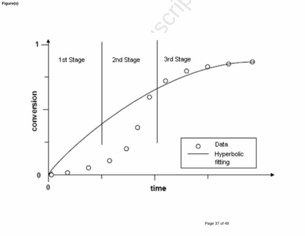
common simplification, the reaction progression has been shown to be sigmoidal and can be

characterised by three stages as shown in Figure 1. The first stage is characterised by an

initial slow rate of reaction; the second by a rapid progression up to approximately 80%

conversion and finally a third stage as equilibrium is approached (Noureddini and Zhu,

1997).

In the first stage, the concentration of oil in the methanol droplets (where the majority of the

catalyst resides) is low, requiring significant agitation to reach saturation levels (Boocock et

al., 1996). During the first stage it is most likely that the rate of mass transfer between the

Page 6 of 49

Accep

ted

Man

uscr

ipt

6

phases is slower than the rate of chemical reaction, thus mass transfer is the rate limiting

factor (Noureddini and Zhu, 1997; Stamenkovic et al., 2007).

In the second stage, the reaction rate rapidly increases. Stamekovic et al. (2007; 2008),

observed that this increase coincided with a reduction in droplet size. As the droplet size

decreases, the surface area of the polar phase and thus the mass transfer rate increases,

explaining the sudden jump in reaction rate. The reaction medium during this stage has been

described by some as a pseudo single phase emulsion (Ma et al., 1999; Zhou and Boocock,

2006) . Different authors have attributed the self-enhanced mass transfer rate to the surfactant

action of the reaction intermediates (Boocock et al., 1998; Stamenkovic et al., 2007), while

others have attributed it to the solvent properties of FAME (Noureddini and Zhu, 1997).

In the third step, the reaction rate rapidly curtails as equilibrium is approached. It is proposed

that this sudden fall is due to the breaking of the single phase emulsion as glycerol is formed,

resulting in the catalyst preferentially dissolving in the polar phase. With almost all of the un-

reacted glycerides residing in the non-polar phase this results in a very slow approach to

equilibrium. It is therefore proposed that in the final stage, it is the solubility of components

and not the rate of mass transfer which limits the reaction rate. This was also observed in the

reverse reaction (glycerolysis of FAME) (Kimmel, 2004; 2006).

In most industrial operations the methanolysis reaction is conducted between 50°C and 70°C

with significant mixing. Under these conditions it is reasonable to assume that the effect of

mass transfer limitations in the first stage is negligible (Noureddini and Zhu, 1997; Vicente et

al., 2005a). In the second stage, the absence of mass transfer limitations allows the reaction to

be treated as a single phase. Consequently, both the first and second stages of the reaction can

be adequately described by second order kinetics models available in the literature that ignore

the multiphase behaviour of the reaction.

This second order model could be extended to the third reaction step, however, the high

difference in density can result in the glycerol laden polar phase separating from the non-

Page 7 of 49

Accep

ted

Man

uscr

ipt

7

polar phase causing the reaction to cease prematurely. This is especially true for tubular

reactors in which the flow can stratify on long straight runs with insufficient turbulence.

CFD modeling was identified as an excellent tool to investigate the flow behavior of the two

phases in tubular reactors during the final stage of the reaction. The development of such a

CFD model allows different reactor designs (diameter and length) and operating conditions

(flow-rate) to be easily trialed. The remainder of this paper firstly introduces the experimental

work conducted on a tubular reactor and secondly provides details on the CFD model

developed to represent the biphasic flow in the reactor.

2 Experimental Method and Materials

For the purpose of developing the CFD model it was identified that viscosity and density data

for both phases would be required as well as flow visualisation results to verify the outputs of

the model.

2.1 Viscosity and Density

To measure the viscosity and density properties, a sample of the reaction medium was taken

and allowed to settle. The viscosity and density of each phase were measured from 30°C to

70°C at 3°C or 5°C increments using a Stabinger viscometer. The viscosity measurements are

reproducible to 0.35% of the measurement, and density measurements are reproducible to

0.0005g/cm3. The temperature was maintained to within 0.005°C.

2.2 Flow Visualisation

To provide qualitative direction and validation for the CFD model, a novel high temperature

and pressure tubular reactor developed by Bluediesel PTY LTD was used to conduct flow

visualisation studies. The reactor consists of multiple straight runs (5.8m) followed by tight

(180°) bends. Before the tubular reactor a mixing tank is present in which the first two stages

of the reaction rapidly occur. As a result, the reactants typically enter the tubular reactor 80%

reacted and thus in the final stage of the reaction.

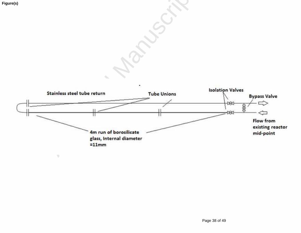
To allow visualisation of the fluid flow, a 4m run of thick walled (2.5mm) borosilicate glass

tube was plumbed into the midpoint of the reactor via three isolating valves. This tube had an

Page 8 of 49

Accep

ted

Man

uscr

ipt

8

internal diameter of 11mm which was required to achieve a pressure rating in excess of 300

psi. Figure 2 depicts the experimental equipment with the thick lines representing the glass

tube, the thin lines representing the stainless steel tube and the double vertical lines the

unions between lengths. To record the flow visualisation results, a high resolution digital

video camera was setup on a tripod adjacent to the glass tubing. This video camera was used

to record the flow of the coloured liquid against a white backdrop.

3 Results

3.1 Viscosity and Density

Viscosity and density of the non-polar and polar phases of the canola and coconut reaction

mixtures are shown in Tables 2 through to 5, respectively. Temperature correlations for

density and viscosity are provided in Tables 6 and 7, respectively.

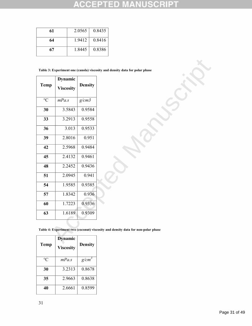
The results in Tables 2 to 5 show the viscosity and density decreasing with increasing

temperature as expected. The density of the two non-polar phases (Tables 2 and 4) are very

similar, while the viscosity is noticeably higher in the canola mixture because of the longer

average carbon chain length of the fatty acids (Krisnangkura et al., 2006).

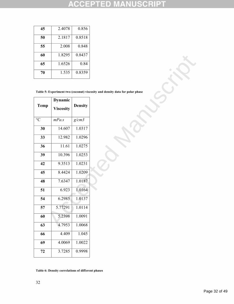
The very different results for the two polar phases in Tables 3 and 5 can be attributed to the

different methanol contents in the two experiments. In the first experiment (canola) the

methanol content was higher as the reaction was originally charged with a high methanol to

oil ratio and it was fresh. In the second experiment (coconut) the methanol content was low

as it was originally charged with a low methanol to oil molar ratio (5:1) and it had been

sitting for six months between the last use of the plant and the experimental run. The low

methanol content in the coconut glycerol phase caused the density and viscosity

measurements to be significantly higher than those for the canola glycerol phase.

3.1.1 Density

Variations of liquid density with temperature are commonly correlated using the linear

relationship shown in Equation 1 (Coupland and McClements, 1997; Liew et al., 1992).

Where ρ, ρ0 and ρ1 are densities measured in kg/m3 and T is temperature in degrees Celsius.

Page 9 of 49

Accep

ted

Man

uscr

ipt

9

T10

Equation 1: Density correlation

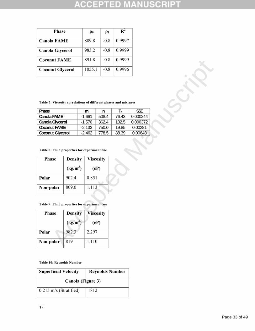
Table 6 contains the linear correlations for the data shown in Tables 2 to 5; with the square of

the residuals (R2) confirming the linear correlation is a good fit for the data sets.

3.1.2 Viscosity

Liew et al., (1992) correlated liquid viscosity with temperature using the relationship shown

in Equation 2 (μ is viscosity, T is temperature, m,n and T0 are correlation coefficients

determined by fitting the curve to the data). This relationship was fitted to the data using the

Fminsearch function in Matlab, which varied the three coefficients (m,n and T0) to minimize

the sum of the square of the errors (SSE). The values of the coefficients are shown in Table 7.

0

logTT

nm

Equation 2: Viscosity correlation

These correlations were extrapolated to the reaction midpoint temperature (Table 1) for each

experiment to provide the viscosity and density values shown in Tables 8 and 9.

3.2 Flow Visualisation

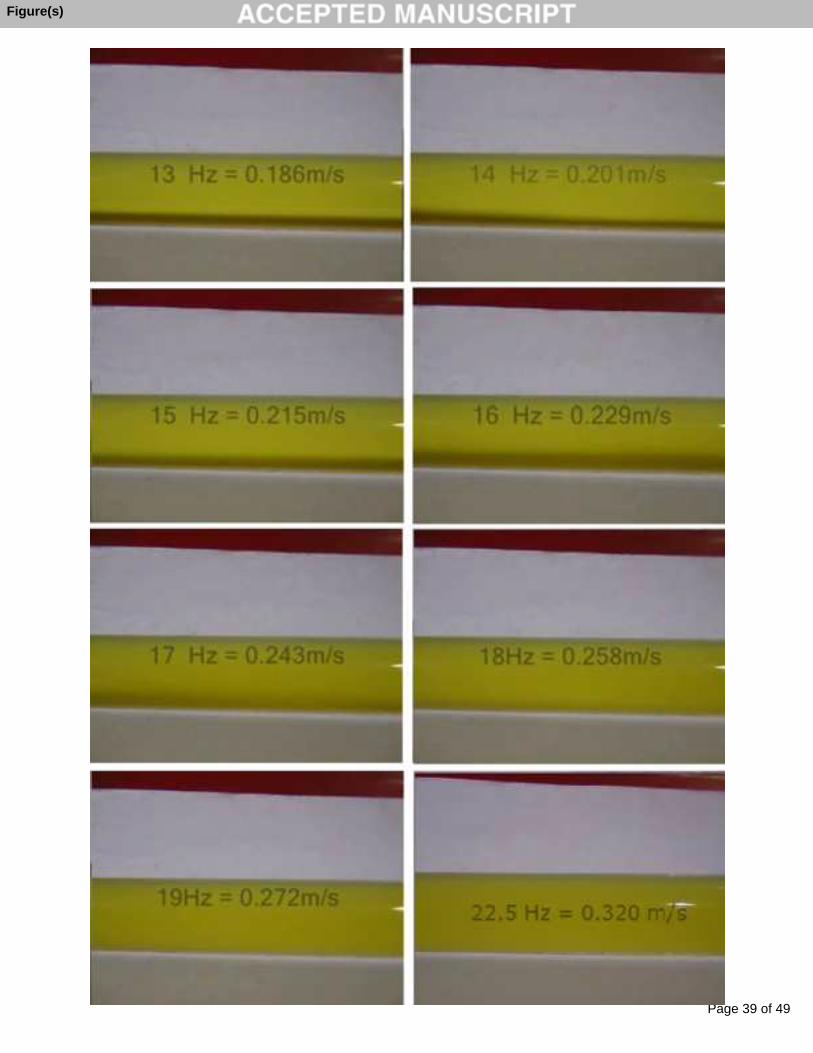
The flow visualisation results are summarised in Table 1, with the associated snapshots from

the results videos contained in Figures 3 and 4, respectively (the full videos are available in

the supplementary material). The results in the first row are for refined canola oil (<0.1%

FFA) which was reacted with methanol at a ratio of 6:1 and a catalyst concentration

(Potassium methylate) of 0.75% weight of oil. Food colouring (red, 50ml) was added to the

mixing tank before the reactor to provide a clear distinction between the polar and non-polar

phases.

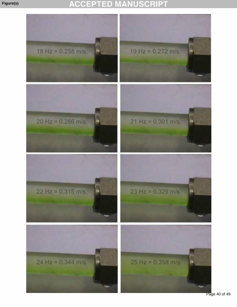
The second row of Table 1 contains the experimental conditions for Refined Bleached Dried

(RBD) coconut oil (Procter and Gamble, Australia) which had been reacted for a long period

Page 10 of 49

Accep

ted

Man

uscr

ipt

10

of time with methanol at a ratio of 5:1 and catalyst concentration (Sodium Methylate) 0.5%

weight of oil. Food colouring (green, 50ml) was added to the mixing tank before the reactor

to provide a clear distinction between the polar and non-polar phase. The food colouring

preferentially dissolves in the polar phase and provides a simple but effective method for

multiphase flow visualisation (Zhou and Boocock, 2006).

The flow-rate was controlled using a variable speed drive on the high pressure pump that

drove the reaction medium through the reactor. The superficial flow velocities for each case

were calculated using the specific volumetric flow-rate of the pump (4.9L/Hz) and the tube

diameter (0.011m).

Figures 3 and 4 contain snapshots taken from the visualisation results of experiments 1 and 2

shown in Table 1. In both cases there is a transition from horizontal stratified flow to

dispersed flow. For the canola oil feedstock, the transition took place between 0.26 and

0.27m/s, while for the coconut oil feedstock the transition took place between 0.34 and 0.36

m/s. The significant difference in transition velocities can be attributed to the different

methanol content in each case. The increased methanol content has a very limited co-

solvency effect between the glycerol and methyl esters (Negi et al., 2006), however, it

significantly reduces the density and viscosity of the glycerol phase (see the difference in

density between the canola and coconut glycerol phases in Tables 3 and 5, respectively). This

effect reduces the turbulent energy required to disperse the polar phase into the non-polar

phase and thus explains the lower velocity required to achieve dispersion in the canola based

results.

It was observed that the transition from stratified to dispersed flow occurs via the propagation

of longitudinal waves with wavelengths greater than the reactor diameter. This is the same

mechanism that occurs in stratified water and oil flows with the crashing waves releasing

droplets which leads to dispersion of the phases at increasing velocities (Al-Wahaibi and

Angeli, 2007; Al-Wahaibi et al., 2007). This is most clearly shown in the stills from 12Hz to

18Hz in experiment 2 (Figure 4) due to the clear distinction between phases.

Page 11 of 49

Accep

ted

Man

uscr

ipt

11

4 Discussion

4.1 Flow Transition and Reynolds number

The flow visualisation results in Figures 3 and 4 demonstrate that the two-phase flow regime

varies significantly with flow velocity. At low velocities, the flow stratifies while at higher

velocities the polar phase becomes dispersed in the continuous non-polar phase. The first is

undesirable as it limits mass transfer, while the second represents the intended design with

each phase having access to the other and component solubility and reaction equilibrium

being the only limitations in the final stage of reaction. When considering various tubular

reactor designs (diameter and length) and operating conditions (flow-rate) it is necessary to

predict the flow regime to prevent stratification.

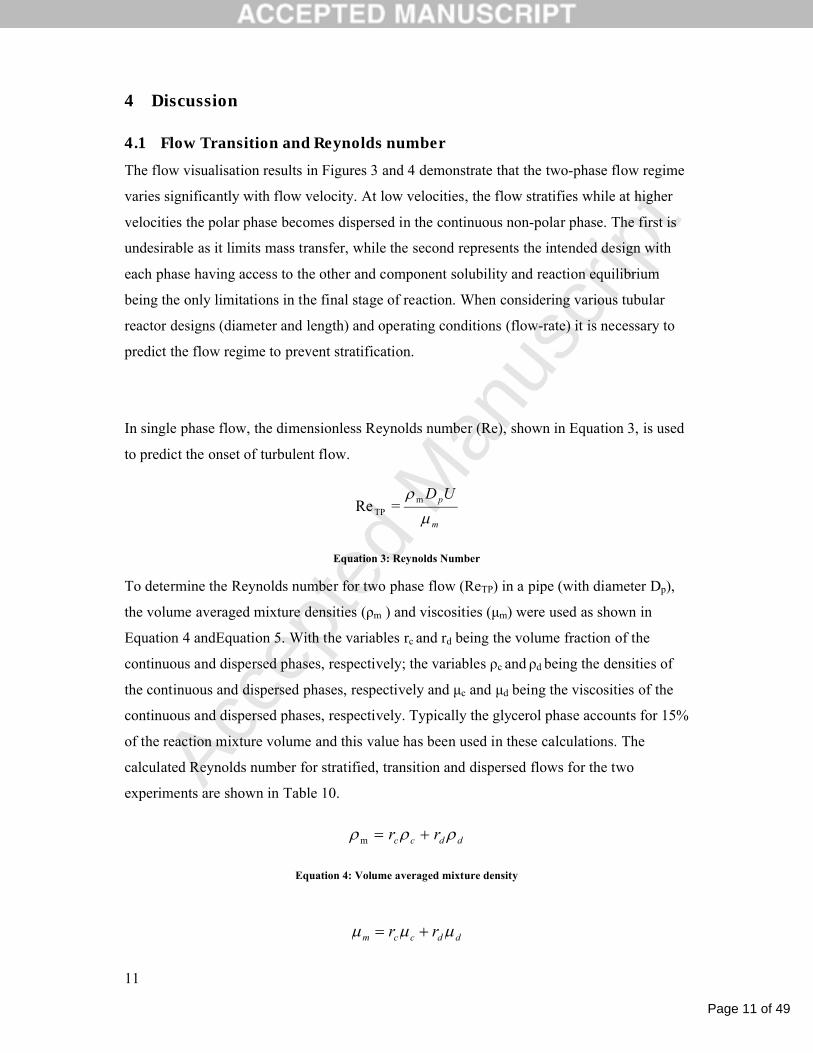
In single phase flow, the dimensionless Reynolds number (Re), shown in Equation 3, is used

to predict the onset of turbulent flow.

m

pUD

m

TP =Re

Equation 3: Reynolds Number

To determine the Reynolds number for two phase flow (ReTP) in a pipe (with diameter Dp),

the volume averaged mixture densities (ρm ) and viscosities (μm) were used as shown in

Equation 4 andEquation 5. With the variables rc and rd being the volume fraction of the

continuous and dispersed phases, respectively; the variables ρc and ρd being the densities of

the continuous and dispersed phases, respectively and μc and μd being the viscosities of the

continuous and dispersed phases, respectively. Typically the glycerol phase accounts for 15%

of the reaction mixture volume and this value has been used in these calculations. The

calculated Reynolds number for stratified, transition and dispersed flows for the two

experiments are shown in Table 10.

ddcc rr m

Equation 4: Volume averaged mixture density

ddccm rr

Page 12 of 49

Accep

ted

Man

uscr

ipt

12

Equation 5: Volume averaged mixture viscosity

Spriggs (1973) and many other authors suggest that true laminar flow exists below a

Reynolds number of 2000, with a transition from laminar to turbulent flow between Reynolds

numbers of 2000 and 3000. By examining the calculated results in Table 10 it is clear that

this criterion provides a somewhat reasonable match with the transition to turbulent flow in

this case, with numbers above 2000 corresponding with the polar phase being dispersed as

recorded in Figures 3 and 4.

The use of Reynolds number provides a reasonable initial design estimate of the flow regime

at a particular design velocity for tubular reactors. Unfortunately, the Reynolds number

cannot capture the behaviour of the flow in more complex reactor geometries. The

application of CFD modeling to this particular problem will provide further insight into the

effect of reactor design on flow regime and a foundation for other more complicated reactor

geometries.

5 CFD Model Development

There are two distinct approaches to modeling two phase flow, the first referred to as

Eulerian-Langrangian and the second as Eulerian-Eulerian. In the former, the dispersed phase

is treated as discrete particles that interact with the continuous phase, while in the latter both

phases are modelled in the Eulerian framework with both having the same velocity in a

defined control volume (mesh). The former, called Lagrangian particle tracking in ANSYS

CFX 12, is suitable for low dispersed phase volume fractions, while the latter approach is

suitable to higher dispersed phase volume fractions. The Eulerian-Eulerian approach was

selected for the modeling of biodiesel reactors as the dispersed polar phase volume fraction

remains virtually constant at 15% in the final stage of the reaction.

The model was setup as an inhomogeneous multiphase problem as each phase had its own

flow field. In this approach simulation of the flow was carried out by solving the governing

Page 13 of 49

Accep

ted

Man

uscr

ipt

13

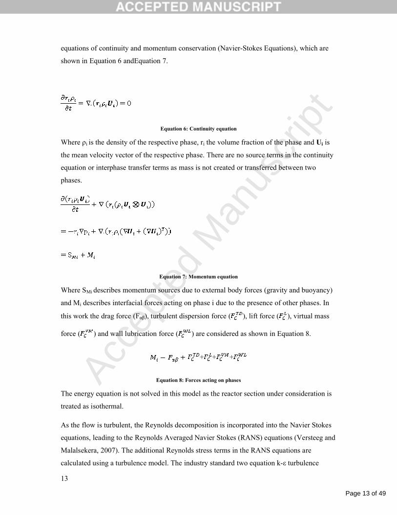
equations of continuity and momentum conservation (Navier-Stokes Equations), which are

shown in Equation 6 andEquation 7.

Equation 6: Continuity equation

Where ρi is the density of the respective phase, ri the volume fraction of the phase and Ui is

the mean velocity vector of the respective phase. There are no source terms in the continuity

equation or interphase transfer terms as mass is not created or transferred between two

phases.

Equation 7: Momentum equation

Where SMi describes momentum sources due to external body forces (gravity and buoyancy)

and Mi describes interfacial forces acting on phase i due to the presence of other phases. In

this work the drag force (Fαβ), turbulent dispersion force ( ), lift force ( ), virtual mass

force ( ) and wall lubrication force ( ) are considered as shown in Equation 8.

+ + +

Equation 8: Forces acting on phases

The energy equation is not solved in this model as the reactor section under consideration is

treated as isothermal.

As the flow is turbulent, the Reynolds decomposition is incorporated into the Navier Stokes

equations, leading to the Reynolds Averaged Navier Stokes (RANS) equations (Versteeg and

Malalsekera, 2007). The additional Reynolds stress terms in the RANS equations are

calculated using a turbulence model. The industry standard two equation k-ε turbulence

Page 14 of 49

Accep

ted

Man

uscr

ipt

14

model implemented in ANSYS CFX was used for this simulation as it is well suited to the

flow regime present (ANSYS, 2009).

The physical properties (viscosity and density) for the non-polar and polar phases for the two

experiments were taken from Tables 8 and 9, respectively. These were assumed to remain

constant due to the isothermal operation of the reactor section under consideration.

The difference in density between the two phases necessitates the modeling of buoyancy.

Buoyancy is modelled on the density difference of the two phases and results in the addition

of a source term to the momentum equation (SM=(ρ- ρref)g). The reference density was set

equal to the continuous phase density to simplify the form of the momentum equation

(ANSYS, 2009).

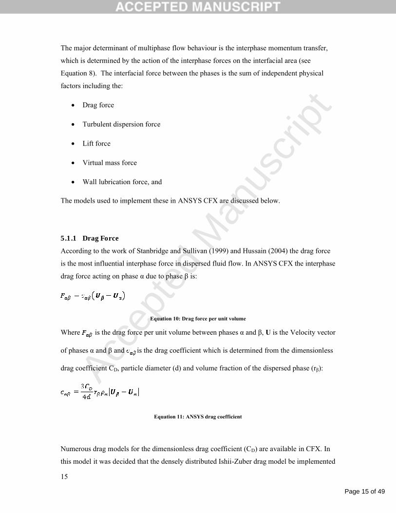
The transfer of momentum between phases is dependent on the interphase forces acting on

the interfacial area per unit volume between phase α and β (Aαβ) (ANSYS, 2009). Due to the

dispersed nature of the polar phase, the particle model was implemented in CFX which

assumes the dispersed phase consists of sphere particles with a mean diameter dβ. This

assumption allows the interfacial area to be calculated from the volume fraction (rβ)

according to Equation 9:

d

rA

6

Equation 9: Interfacial area between phases (ANSYS, 2009)

The mean droplet diameter (dβ) for the polar phase was set as 0.055mm on the basis of the

work of Stamenkovic et al., (2007; 2008) in which experimental measurement showed a

constant value between 0.05 and 0.06mm in the final stage of the reaction.

Page 15 of 49

Accep

ted

Man

uscr

ipt

15

The major determinant of multiphase flow behaviour is the interphase momentum transfer,

which is determined by the action of the interphase forces on the interfacial area (see

Equation 8). The interfacial force between the phases is the sum of independent physical

factors including the:

Drag force

Turbulent dispersion force

Lift force

Virtual mass force

Wall lubrication force, and

The models used to implement these in ANSYS CFX are discussed below.

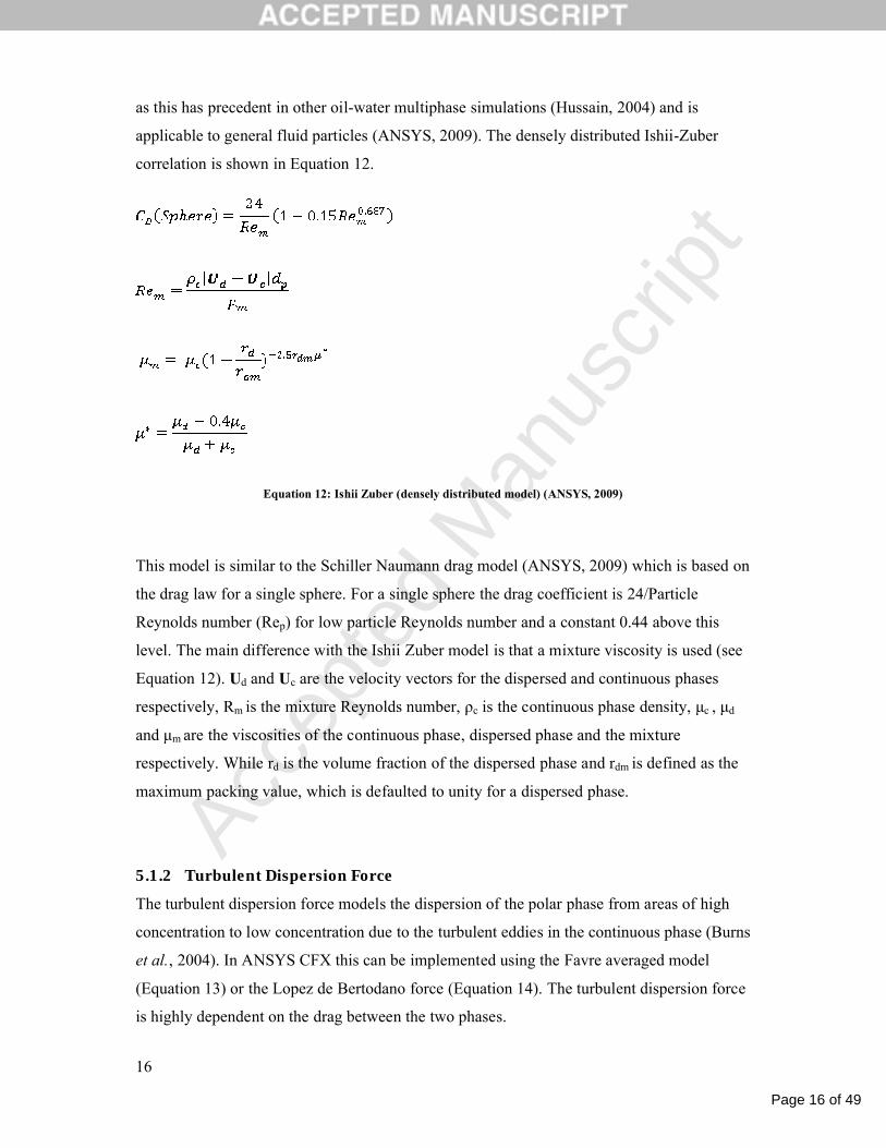
5.1.1 Drag Force

According to the work of Stanbridge and Sullivan (1999) and Hussain (2004) the drag force

is the most influential interphase force in dispersed fluid flow. In ANSYS CFX the interphase

drag force acting on phase α due to phase β is:

Equation 10: Drag force per unit volume

Where is the drag force per unit volume between phases α and β, U is the Velocity vector

of phases α and β and is the drag coefficient which is determined from the dimensionless

drag coefficient CD, particle diameter (d) and volume fraction of the dispersed phase (rβ):

Equation 11: ANSYS drag coefficient

Numerous drag models for the dimensionless drag coefficient (CD) are available in CFX. In

this model it was decided that the densely distributed Ishii-Zuber drag model be implemented

Page 16 of 49

Accep

ted

Man

uscr

ipt

16

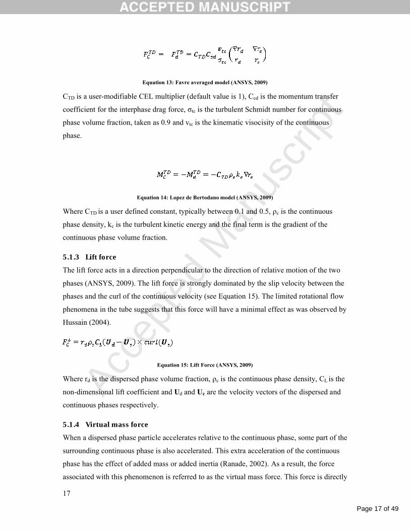
as this has precedent in other oil-water multiphase simulations (Hussain, 2004) and is

applicable to general fluid particles (ANSYS, 2009). The densely distributed Ishii-Zuber

correlation is shown in Equation 12.

Equation 12: Ishii Zuber (densely distributed model) (ANSYS, 2009)

This model is similar to the Schiller Naumann drag model (ANSYS, 2009) which is based on

the drag law for a single sphere. For a single sphere the drag coefficient is 24/Particle

Reynolds number (Rep) for low particle Reynolds number and a constant 0.44 above this

level. The main difference with the Ishii Zuber model is that a mixture viscosity is used (see

Equation 12). Ud and Uc are the velocity vectors for the dispersed and continuous phases

respectively, Rm is the mixture Reynolds number, ρc is the continuous phase density, μc , μd

and μm are the viscosities of the continuous phase, dispersed phase and the mixture

respectively. While rd is the volume fraction of the dispersed phase and rdm is defined as the

maximum packing value, which is defaulted to unity for a dispersed phase.

5.1.2 Turbulent Dispersion Force

The turbulent dispersion force models the dispersion of the polar phase from areas of high

concentration to low concentration due to the turbulent eddies in the continuous phase (Burns

et al., 2004). In ANSYS CFX this can be implemented using the Favre averaged model

(Equation 13) or the Lopez de Bertodano force (Equation 14). The turbulent dispersion force

is highly dependent on the drag between the two phases.

Page 17 of 49

Accep

ted

Man

uscr

ipt

17

Equation 13: Favre averaged model (ANSYS, 2009)

CTD is a user-modifiable CEL multiplier (default value is 1), Ccd is the momentum transfer

coefficient for the interphase drag force, σtc is the turbulent Schmidt number for continuous

phase volume fraction, taken as 0.9 and vtc is the kinematic visocisity of the continuous

phase.

Equation 14: Lopez de Bertodano model (ANSYS, 2009)

Where CTD is a user defined constant, typically between 0.1 and 0.5, ρc is the continuous

phase density, kc is the turbulent kinetic energy and the final term is the gradient of the

continuous phase volume fraction.

5.1.3 Lift force

The lift force acts in a direction perpendicular to the direction of relative motion of the two

phases (ANSYS, 2009). The lift force is strongly dominated by the slip velocity between the

phases and the curl of the continuous velocity (see Equation 15). The limited rotational flow

phenomena in the tube suggests that this force will have a minimal effect as was observed by

Hussain (2004).

Equation 15: Lift Force (ANSYS, 2009)

Where rd is the dispersed phase volume fraction, ρc is the continuous phase density, CL is the

non-dimensional lift coefficient and Ud and Uc are the velocity vectors of the dispersed and

continuous phases respectively.

5.1.4 Virtual mass force

When a dispersed phase particle accelerates relative to the continuous phase, some part of the

surrounding continuous phase is also accelerated. This extra acceleration of the continuous

phase has the effect of added mass or added inertia (Ranade, 2002). As a result, the force

associated with this phenomenon is referred to as the virtual mass force. This force is directly

Page 18 of 49

Accep

ted

Man

uscr

ipt

18

proportional to the relative acceleration between the two phases (bracketed terms in Equation

16). In this model it was expected that this force would have a limited impact on the

simulation as the dispersed phase is carried along in the continuous phase.

Equation 16: Virtual mass force (ANSYS, 2009)

Where rd is the dispersed phase volume fraction, ρc is the continuous phase density, CVM is

the virtual mass coefficient and Ud and Uc are the velocity vectors of the dispersed and

continuous phases respectively.

5.1.5 Wall lubrication force

The wall lubrication force is intended to model the phenomena observed when bubbles

concentrate close but not immediately adjacent to walls. This is particularly applicable to air

bubbles in liquid flow and has been shown to have little effect in previous liquid-liquid flow

work (Hussain, 2004).

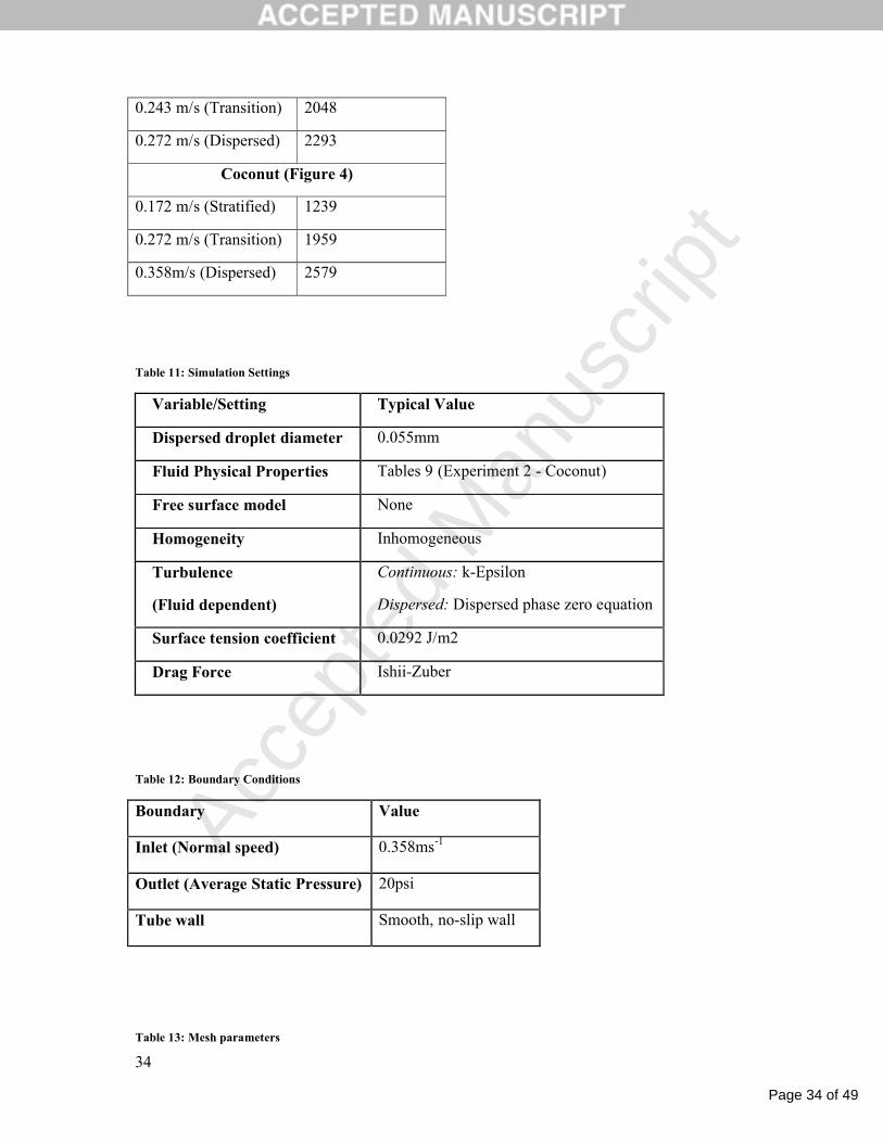
With this background a base case simulation was developed to be a basis for systematic

parametric investigation – the inputs for this base case are summarised in Table 11. The

surface tension coefficient mentioned in this table was required for the Ishii-Zuber correlation

and was taken from Allen (1999).

The boundary conditions for this base case are summarised in Table 12. For the studies

performed, the inlet turbulence intensity was set at 5% which is typical for pipe flows

(Abraham et al., 2008). The outlet pressure was set at 20 psi.

5.1.6 Geometry, mesh and solver control

The flow domain of the biodiesel reactor was developed in ANSYS Design Modeller by

extruding a sketch with the internal diameter (11mm) of the reactor tube. This flow domain

mimics the experimental setup. A three dimensional mesh of this flow domain was developed

Page 19 of 49

Accep

ted

Man

uscr

ipt

19

using the ANSYS meshing tool in Workbench 12. The nature of the tube lends itself to sweep

meshing with the level of refinement determined by the face mesh controls and the number of

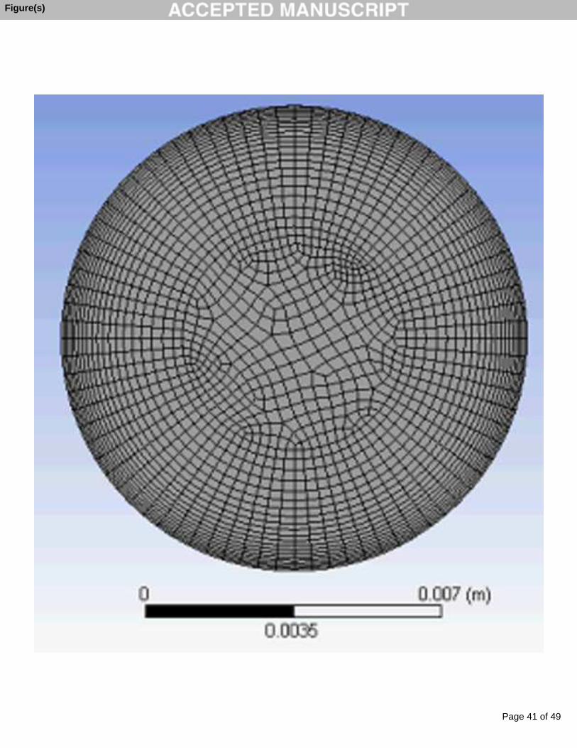
sweep divisions. A mesh independence study was conducted for both pure tetrahedral face

meshes and tetrahedral meshes with inflation at the tube walls (de Boer, 2010). The study

resulted in the choice of the mesh shown in Figure 5 that gave reasonable solution times with

high accuracy. Further refinement provided negligible increases in resolution of the base case

for substantial increases in solution time. Details of the meshing parameters are summarised

in Table 13.

The level of mesh refinement is also affected by the number of sweep divisions in the mesh

(these determine the thickness of the face mesh cells throughout the volume). To minimise

solution time 200 divisions was used for the 4m tube geometry. To further reduce

computational time, tubes are typically split in half and a symmetry plane is inserted

(Hussain, 2004). This halves the number of control volumes and therefore essentially halves

the number of equations to be solved at each iteration. It was found that the use of a

symmetry plane had minimal effect on the solution (de Boer, 2010) and as a result a half tube

was modelled to cut the solution time in half. Using the mesh with the face pattern shown in

Figure 5 and 200 swept divisions the total element count was 189,200. The solver control

settings were also investigated on the base case to identify values that would provide

sufficient accuracy in less than 3 hrs. Sufficient accuracy was defined when further tightening

of residuals and imbalances delivered a change in the polar phase volume fraction of less than

1%. The identified settings are listed below:

Time scale – 0.3s (Reduced to 0.01 when using the Turbulent Dispersion force)

Advection Scheme – High Resolution

Imbalances – 0.01

Residuals – 0.0001

Using the above mesh and solver settings, the solution time was approximately three hours on

four cores of a dual, quad core cpu (3GHz Xeon) server.

Page 20 of 49

Accep

ted

Man

uscr

ipt

20

6 Results

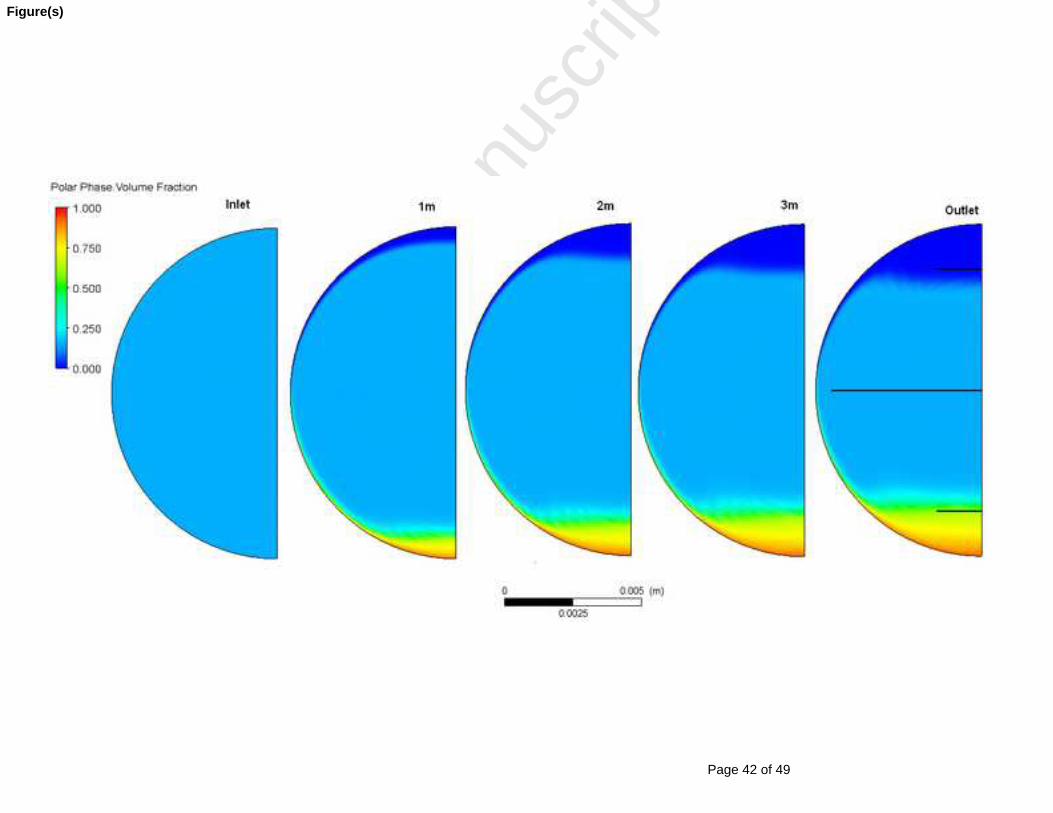
Implementing the base case simulation (Table 11) using the aforementioned mesh and solver

conditions yielded the simulation results shown in Figure 6. The plots show the polar phase

volume fraction dispersed across the face of the reactor tube at different points. The polar

phase volume fraction was used as a qualitative simulation result for comparison with the

flow visualisation results in Figures 3 and 4. The black lines were used to average the polar

phase volume fraction across the line for more accurate comparison when results were not

visibly different.

These results clearly indicate that the flow is stratifying where the results in Figure 4 show

the flow is highly dispersed. To evaluate the adequacy of the chosen physical models and

assess the sensitivity of the model to inputs, parametric studies were performed by changing

the following variables independently in the base case (Table 11):

Droplet diameter: 0.04mm to 0.07mm

Inlet Velocity: 0.1m/s to 1m/s

Density and Viscosity: 5 and 10% either side of the base case values

Lift Force: Lift coefficient between 0.1 and 10

Virtual Mass Force: Virtual mass coefficient between 0.1 and 10

Wall Lubrication Force: Tomiyama with pipe diameter = 0.011m

Turbulent Dispersion force: CTD between 0.25 and 1

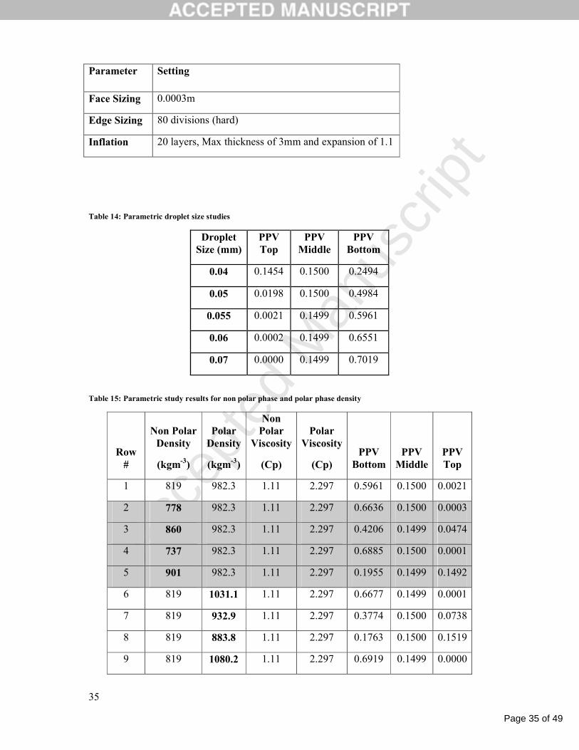
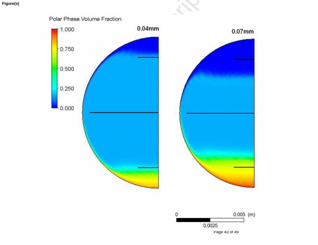
6.1 Droplet Diameter

The dispersed (polar) phase droplet diameter is a key variable in multi-phase simulations as it

determines the interfacial area for momentum, mass and energy transfer and can have a

significant effect on simulation results. Table 14 summarises the results of parametric droplet

sizes between 0.04 and 0.07mm, while Figure 7 compares the polar phase volume fraction at

the outlet of the simulations using the smallest and largest droplet sizes. Both Table 14 and

Figure 7 show that stratification increases with increasing droplet size. As the droplet

Page 21 of 49

Accep

ted

Man

uscr

ipt

21

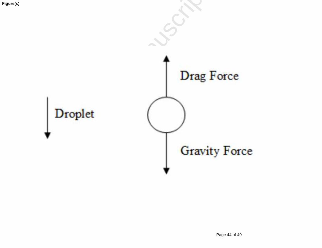
diameter is increased, both the drag coefficient used by ANSYS CFX and the interfacial area

reduce (see Equations 7, 8 and 9), ultimately reducing the drag force. As a result, the net

effect of the gravitational force is greater (see Figure 8) causing greater stratification (Figure

7).

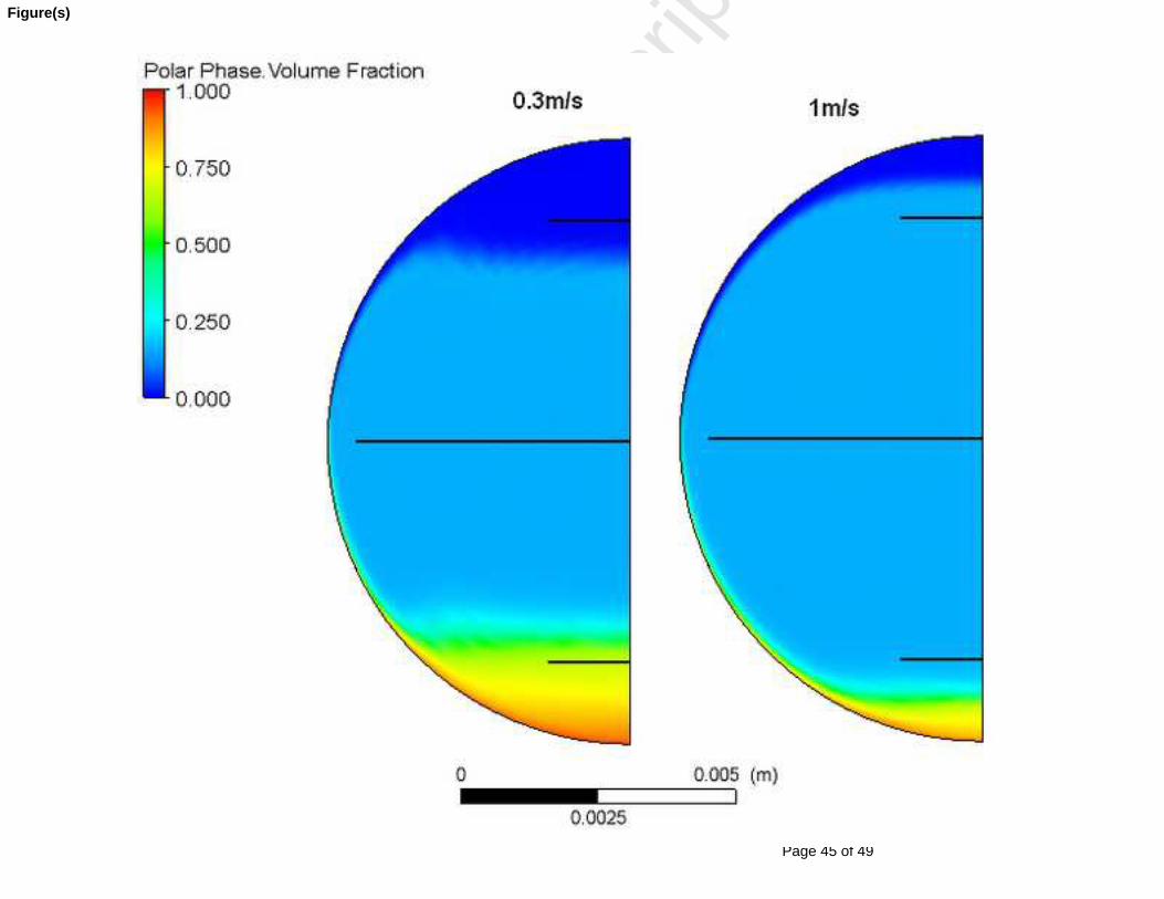
6.2 Inlet velocity

In pipe flow, inlet velocity is one of the key variables affecting the level of turbulence. In

multi-phase simulations a higher velocity will result in increased turbulence and a higher

level of dispersion. The lower velocities (<0.3ms-1) did not converge, as the flow regime in

these simulations is no longer dispersed but instead stratified. Figure 9 shows that an increase

in velocity reduces the level of stratification, however, even at the unrealistic velocity of 1

m/s the stratification is still present.

6.3 Density and viscosity

To examine the effect of density and viscosity measurement errors, systematic studies were

conducted into the density and viscosity of the phases (5% or 10% on base case) with results

shown in Tables 15 and 16, respectively. In these tables the bold type indicates which

variables are being altered and the shading is used to clarify the distinction between polar and

non-polar phases. It was found that density (Table 15) had a greater effect than viscosity

(Table 16) with an 83% change in the bottom polar phase volume fraction (PV bottom)

across the non-polar density variations while only a 12% change in the same variable for the

changes in viscosity. The effect of density was similar for both phases, that is, a reduction of

10% in the polar phase density (Table 15 row 8) gave similar results to a 10% increase in

non-polar phase density (Table 15 row 5). This can be attributed to the buoyancy force which

is driven by the density difference between the two phases. The higher the relative density of

the polar phase, the greater the stratification and therefore the PV bottom value will be

higher.

The influence of density on the level of stratification aligns closely with the experimental

observations recorded earlier. Unlike the base case (coconut oil – experiment 2) which had a

Page 22 of 49

Accep

ted

Man

uscr

ipt

22

density difference of 163.3 kg/m3 (Table 9) the canola oil feedstock (experiment 1) had a

density difference of only 93.4 kg/m3 (Table 8). This lower density difference, caused by

differences in methanol content, resulted in the canola flow visualisation experiment

transitioning from stratified to dispersed at a lower velocity than the coconut case (0.26 m/s

vs 0.36 m/s).

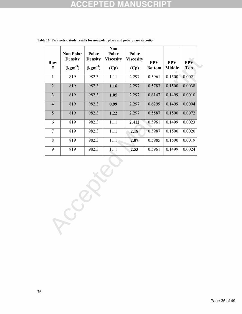
The viscosity on the other hand had a varied effect depending on the phase in which the

viscosity change occurred. As expected, the viscosity of the polar phase droplets had an

almost negligible effect on the results as this viscosity does not affect the majority of the flow

regime. The effect of the continuous phase viscosity on the flow regime was more significant.

The trend, however, was counter-intuitive with a decrease in viscosity increasing

stratification. Intuitively a reduction in viscosity represents a reduction in the viscous

damping forces of the entire flow thus encouraging turbulence and promoting dispersion. In

this case, however, the reduction in viscosity increased stratification. This can be understood

by considering the effect of continuous phase viscosity on the drag coefficient. Examination

of Equation 12 shows that a reduction in the continuous phase viscosity decreases the mixture

viscosity, which increases the particle Reynolds number and thus decreases the drag

coefficient which as discussed in the section on droplet diameter encourages stratification.

The lesser effect of the viscosity in comparison with density is due to the greater magnitude

of the buoyancy force than the drag force.

6.4 Lift, virtual mass and wall lubrication force

The parametric studies conducted on the base case varying the lift, virtual mass and wall

lubrication force had a negligible effect on the polar phase distribution unless the coefficient

was increased to levels that were physically impossible. The limited effect of these interphase

forces observed in this study harmonises with the work of Hussain (2004). The reasons for

the limited effect of these forces are due to the physical nature of this system. Both the slip

velocity and relative phasic accelerations are low and consequently both the lift force and

virtual mass force are negligible. Furthermore, the wall lubrication force is more applicable to

larger diameter bubbles than small diameter droplets.

Page 23 of 49

Accep

ted

Man

uscr

ipt

23

6.5 Turbulent dispersion force

Inclusion of the turbulent dispersion force is particularly relevant for this simulation as it

models the dispersion of particles/droplets caused by the turbulence induced eddies present in

the continuous phase (Burns et al., 2004). Hussain (2004) reported that the turbulent

dispersion force had a strong effect on the simulation results, however, stratification was still

slowly occurring. The turbulent dispersion force strongly depends on the velocity gradients

present in the flow regime which can easily be lost with a mesh that is too coarse.

Examination of the mesh used in Hussain’s study suggests that it was too coarse, especially in

the boundary layer. This lack of resolution is mainly the result of limited computational

resources available 10 years ago.

The greater computational resources available in this study made it possible to further

investigate the effect of the turbulent dispersion force. Initial investigations into this force

were unproductive with both the Lopez de Bertanado and Favre averaged force failing to

converge and simply oscillating at relatively high residual values. This was rectified by

reducing the physical time-step to 0.01s and gradually increasing the turbulent dispersion

coefficient in the Lopez de Bertodano force using the following CEL (CFX Expression

Language) expression:

min(0.5,0.01*aitrn)

Equation 17: Gradual increase of turbulent dispersion coefficient

This ensured that the turbulent dispersion coefficient would build up to the desired value

(0.5) in 0.01 increments per iteration while maintaining stability (aitrn is the CEL variable

name of the iteration number). In Equation 17, the 0.5 represents the actual coefficient used

in the simulation, as after 50 iterations 0.5 is the constant output. The choice of time-step was

based on a systematic process of reducing time step by a factor of 10 until there a converged

and time scale independent solution was achieved. The smaller timescale increases the

stability of the solution and prevents oscillation.

Page 24 of 49

Accep

ted

Man

uscr

ipt

24

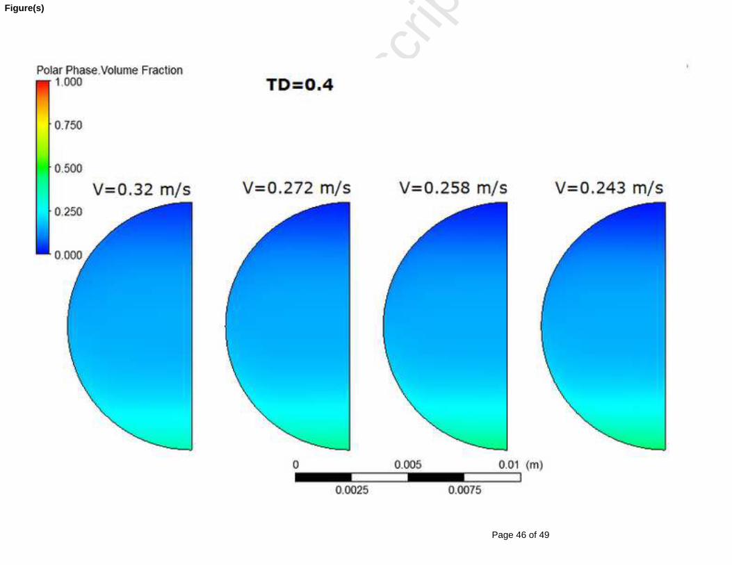
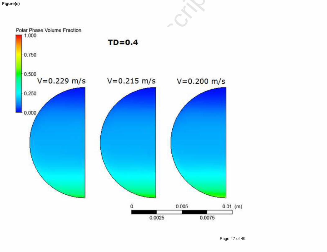
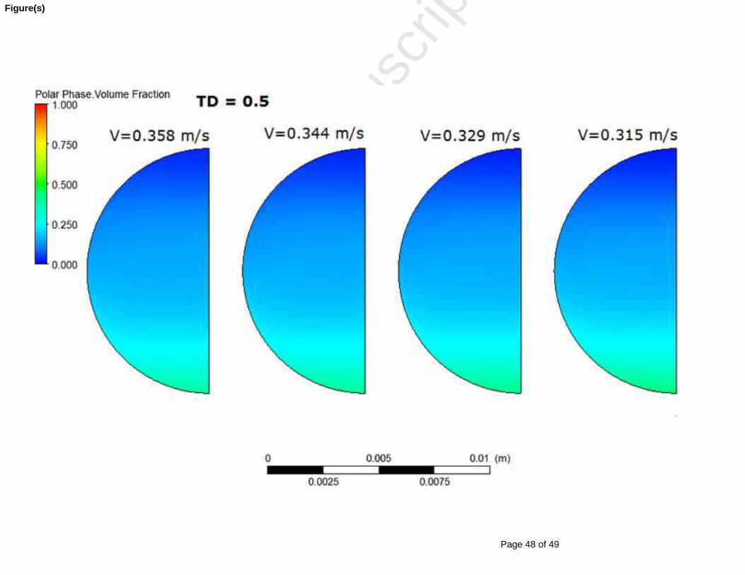
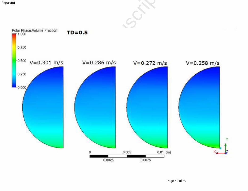
Results of these simulations for experiment one are shown in Figures 10 and 11 and results

for experiment two are shown in Figures 12 and 13. These figures provide plots of the polar

phase volume fraction at the end of the 4m tube in the simulation. At low velocities in both

cases there is clear evidence of stratification with a concentration of the polar phase at the

bottom and an absence at the top of the tube. At higher velocities the polar phase volume

fraction across the face is more uniform with only the slightest amount of stratification

present which can be seen in the corresponding visualisation results.

At the time of writing the CFX 12 solver was unstable when the favre averaged model was

implemented (even with the incremental increase of CTD), however, it is expected that more

current versions of the CFX solver will be able to solve this allowing the model to be more

widely applicable to different reactor geometries.

The comparison of simulation results with experimental results shown in the above figures

confirms the suitability of this CFD model for the prediction of flow dispersion/stratification

in tubular methanolysis reactors. To be conservative a Turbulent Dispersion coefficient of 0.3

should be used in the model to determine whether a particular flow conditions is stratified or

dispersed. Although, this model has not been quantitatively validated, there is enough

qualitative evidence to suggest the model is suitable for determining the flow pattern at a

particular set of conditions.

7 Conclusion

The alignment of the simulation with the corresponding flow visualisation results in Figures 3

and 4 demonstrates that it is possible to qualitatively model the distribution of the polar phase

in the non- polar phase through the inclusion of the drag force and turbulent dispersion force

in the multi-phase model. This achievement advances the application of CFD modeling in

liquid-liquid flows in three ways. Firstly, this model provides a method for predicting the

flow regime of two phase reactions in the production of biodiesel while also laying a

foundation for a comprehensive two phase model of the reaction. Secondly, it provides key

information (phase data and model parameters) for CFD models of other biodiesel reactors

Page 25 of 49

Accep

ted

Man

uscr

ipt

25

(e.g.: Jet reactors, ultrasonic reactors and oscillatory flow reactors). Finally, the alignment of

model outputs with real world data demonstrates that by inclusion of the turbulent dispersion

force it is possible to accurately model any liquid-liquid flow in tubular reactors or pipes.

This fundamental research will provide other researchers and technology developers with

starting points for CFD models of more complicated biodiesel reactor geometries and other

liquid-liquid flows.

Acknowledgements

The authors would like to acknowledge: Australian Government, Murdoch University, Centre

for Research into Energy for Sustainable Transport (CREST) and Bluediesel for their funding

support and provision of infrastructure; LEAP Australia for the provision of ANSYS CFX;

The Australian Lubricant Manufacturing Company (ALMC) for the use of their equipment

and Allira glass blowing for assistance in the experimental design.

Nomenclature

Variables:Re ReynoldsD Pipe diameter (m)d Pipe diameter (m) Density (kg/m3)μ Viscosity (Pa s)U Superficial velocity (m/s)U Velocity vector (m/s)r Volume fractionm Correlation coefficientn Correlation coefficientT Temperature (°C)F ForceA AreaM Lopez De Bertodano forceC Coefficient (dependent on subscripts)

Sub/super script:i Either phase

Page 26 of 49

Accep

ted

Man

uscr

ipt

26

α Phase Aβ Phase Bc Continuous phased Dispersed phasem Mixturep PipeL Lift forceVM Virtual Mass Force

8 References

Abraham, J. P., Sparrow, E. M., & Tong, J. C. K. (2008). Breakdown of Laminar Pipe Flow into Transitional Intermittency and Subsequent Attainment of Fully Developed Intermittent or Turbulent Flow. Numerical Heat Transfer, Part B: Fundamentals: An International Journal of Computation and Methodology, 54(2), 103-115.

Adeyemi, N., Mohiuddin, A. K. M., & Nor, M. I. M. (2013). CFD Modelling of Waste Cooking Oil Transesterification in a Stirred Tank Reactor. World Applied Sciences Journal 21 (Mathematical Applications in Engineering), 151-158.

Akoh, C. C., Chang, S.-W., Lee, G.-C., & Shaw, J.-F. (2007). Enzymatic Approach to Biodiesel Production. Journal of Agricultural and Food Chemistry, 55(22), 8995-9005.

Al-Wahaibi, T., & Angeli, P. (2007). Transition between stratified and non-stratified horizontal oil-water flows. Part I: Stability analysis. Chemical Engineering Science, 62(11), 2915-2928.

Al-Wahaibi, T., Smith, M., & Angeli, P. (2007). Transition between stratified and non-stratified horizontal oil-water flows. Part II: Mechanism of drop formation. Chemical Engineering Science, 62(11), 2929-2940.

Allen, C. A. W. (1999). Predicting the viscosity of biodiesel fuels from their fatty acid ester composition. Fuel, 78, 1319-1326.

ANSYS. (2009). ANSYS CFX-Solver Theory Guide. User Manual. Boocock, D. G. B., Konar, S. K., Mao, V., Lee, C., & Buligan, S. (1998). Fast formation of

high-purity methyl esters from vegetable oils. J. Am. Oil Chem. Soc., 75(9), 1167-1172.

Boocock, D. G. B., Konar, S. K., Mao, V., & Sidi, H. (1996). Fast one phase oil-rich process for the preparation of vegetable oil methyl esters. Biomass and bioenergy, 11(1), 43-50.

Burns, A. D., Frank, T., Hamill, I., & Shi, J.-M. (2004, may 30 - June 4). The Favre Averaged Drag Model for Turbulent Dispersion in Eulerian Multi-Phase Flows.Paper presented at the 5th International Conference on Multiphase Flow, Yokohama, Japan.

Coupland, J. N., & McClements, D. J. (1997). Physical Properties of Liquid Edible Oils. JAOCS, 74(12), 1559-1564.

Darnoko, D., & Cheryan, M. (2000). Kinetics of palm oil transesterification in a batch reactor. JAOCS, 77(12), 1263-1267.

de Boer, K. (2010). Optimised Small Scale Reactor Technology, a new approach for the Australian Biodiesel Industry. (PhD Thesis), School of Engineering and Energy, Murdoch University, Perth, Western Australia.

Page 27 of 49

Accep

ted

Man

uscr

ipt

27

de Boer, K., & Bahri, P. A. (2009). Investigation of Liquid-Liquid two phase flow in biodiesel production. Paper presented at the Seventh International Conference on CFD in the Minerals and Process Industries CSIRO, Melbourne.

de Boer, K., & Bahri, P. A. (2011). Supercritical methanol for fatty acid methyl ester production: A review. Biomass & Bioenergy, 35(3), 983-991. doi: 10.1016/j.biombioe.2010.11.037

Doell, R., Konar, S. K., & Boocock, D. G. B. (2008). Kinetic parameters of homogeneous transmethylation of soybean oil. J. Am. Oil Chem. Soc., 85, 271-276.

Freedman, B., Butterfield, R. O., & Pryde, E. H. (1986). Transesterification kinetics of soybean oil. J. Am. Oil Chem. Soc., 63(10), 1375-1380.

Hussain, S. A. (2004). Experimental and Computational Studies of Liquid-Liquid Dispersed Flows. (PhD Thesis), Univeristy of London, London.

Karmee, S. k., Chandna, D., Ravi, R., & Chadha, A. (2006). Kinetics of base catalyzed transesterification of triglycerides from pongamia oil. J. Am. Oil Chem. Soc., 83(10), 873-877.

Kimmel, T. (2004). Kinetic Investigation of the base-catalysed glycerolysis of Fatty Acid Methyl Esters (PhD Thesis), Technical University of Berlin, Berlin.

Krisnangkura, K., Yimsuwan, T., & Pairintra, R. (2006). An emperical approach in predicting biodiesel viscosity at various temperatures. Fuel, 85, 107-113.

Liew, K. Y., Seng, C. E., & Oh, L. L. (1992). Viscosities and Densities of the Methyl esters of some n-Alkanoic Acids. J. Am. Oil Chem. Soc., 69(2).

Lotero, E., Goodwin, J. G., Bruce, D. A., Suwannakarn, K., Liu, Y., & Lopez, D. E. (2006). The catalysis of Biodiesel synthesis. Catalysis, 19, 41-83.

Ma, F., Clements, D., & Hanna, M. (1999). The effect of mixing on transesterification of beef tallow. Bioresource Technology, 69, 289-293.

Mittelbach, M., & Remschmidt, C. (2006). Biodiesel the comprehensive handbook. Vienna: Martin Mittelbach.

Negi, D. S. (2006). Base Catalyzed Glycerolysis of Fatty Acid Methyl Esters: Investigations Toward the Development of a Continuous Process. (PhD Thesis), Technical University of Berlin, Berlin.

Negi, D. S., Sobotka, F., Kimmel, T., Wozny, G., & Schomacker, R. (2006). Liquid-Liquid Phase Equilibrium in Glycerol-Methanol-Methyl Oleate and Glycerol-Monoolein -Methyl oleate ternary systems. Ind. Eng. Chem. Res., 45, 3693-3696.

Noureddini, H., & Zhu, D. (1997). Kinetics of Transesterification of soybean oil. J. Am. Oil Chem. Soc., 74(11), 1457-1463.

Orifici, L. I., Bahl, C. D., Gely, M. C., Bandoni, A., & Pagano, A. M. (2013). Modeling and Simulattion of the biodiesel production in a pilot continuous reactor. Mecanica Computacional, XXXII, 1451-1461.

Ranade, V. V. (2002). Computational Flow Modelling for Chemical Reactor Engineering(Vol. 5). London: Academic Press.

Sheehan, J., Camobreco, V., Duffield, J., Graboski, M., & Shapouri, H. (1998). Life Cycle inventory of biodiesel and petroleum diesel for use in an urban bus. (NREL/SR-580-24089). National Renewable energy Laboratory Retrieved from http://www.nrel.gov/docs/legosti/fy98/24089.pdf.

Spriggs, H. D. (1973). Comments on Transition from Laminar to Turbulent Flow. Industrial & Engineering Chemistry Fundamentals, 12(3), 286-290. doi: doi:10.1021/i160047a004

Stamenkovic, O. S., Lazic, M. L., Todorovic, Z. B., Veljkovic, V. B., & Skala, D. U. (2007). The effect of agitation intensity on alkali-catalyzed methanolysis of sunflower oil. Bioresource Technology, 98, 2688-2699.

Page 28 of 49

Accep

ted

Man

uscr

ipt

28

Stamenkovic, O. S., Todorovic, Z. B., Lazic, M. L., Veljkovic, V. B., & Skala, D. U. (2008). Kinetics of sunflower oil methanolysis at low temperatures. Bioresource Technology, 99, 1131-1140.

Stanbridge, D., & Sullivan, J. (1999). One example of how offshore oil and industry technology can be of benefit to hydrometallurgy. Paper presented at the Second international conference on CFD in the minerals and process industries (CSIRO), Melbourne, Australia.

Versteeg, H. K., & Malalsekera, W. (2007). An Introduction to Computational Fluid Dynamics (2nd ed.). Harlow: Pearson.

Vicente, G., Martinez, M., & Aracil, J. (2003). Integrated Biodiesel production: A comparison of different homogeneous catalyst systems. Bioresource Technology, 92, 297-305.

Vicente, G., Martinez, M., & Aracil, J. (2005a). Optimization of Brassica carinata oil methanolysis for biodiesel production. J. Am. Oil Chem. Soc., 82(12), 899-904.

Vicente, G., Martinez, M., Aracil, J., & Esteban, A. (2005b). Kinetics of Sunflower Oil Methanolysis. Ind. Eng. Chem. Res., 44, 5447-5454.

Wang, W.-C., Natelson, R. H., Stikeleather, L. F., & Roberts, W. L. (2012). CFD Simulation of transient stage of continuous countercurrent hydrolysis of canola oil. Computers and chemical engineering, 43, 108-119.

Wulandani, D., Ilham, F., Hagiwara, S., & Nabetani, H. (2012). The effect of obstacle types on the behavior of methanol bubble in the triglyceride within the column reactor by using CFD simulation. Journal of Mechanical Engineering and Technology, 4(2), 61-68.

Zhou, W., & Boocock, D. G. B. (2006). Phase behavior of the base catalyzed transesterification of soybean oil. J. Am. Oil Chem. Soc., 83(12), 1041-1045.

Page 29 of 49

Accep

ted

Man

uscr

ipt

29

Development and Validation of a two phase CFD

model for tubular Biodiesel Reactors

Karne de Boer2 and Parisa A. Bahri

School of Engineering and Information Technology, Murdoch University, Perth, Western Australia

1 Figures

Please see the correspondingly named tiff files submitted with this article

Figure 1: Sigmoidal reaction progression

Figure 2: Flow Visualisation Equipment

Figure 3: Experiment one visualisation results

Figure 4: Experiment two visualisation results

Figure 5: Chosen face mesh

Figure 6: Base case simulation results – developing flow profile

Figure 7: Comparison of droplet size simulation results

Figure 8: Forces acting on a falling polar phase droplet

Figure 9: Comparison of results for velocity parametric studies

Figure 10: Simulation results for Canola at velocities 0.243-0.32m/s with a TD of 0.4

Figure 11: Simulation results for Canola at velocities 0.2-0.229m/s with a TD of 0.4

Figure 12: Simulation results for Coconut at velocities 0.358 – 0.315m/s with a TD of 0.5

Figure 13: Simulation results for Coconut at velocities 0.258 – 0.301m/s with a TD of 0. 5

2 Tables

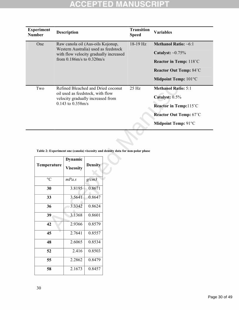
Table 1: Summary of experimental conditions

2 Corresponding author Email: karne@regenerateindustries.com

Page 30 of 49

Accep

ted

Man

uscr

ipt

30

Experiment Number

DescriptionTransition Speed

Variables

One Raw canola oil (Aus-oils Kojonup, Western Australia) used as feedstock with flow velocity gradually increased from 0.186m/s to 0.320m/s

18-19 Hz Methanol Ratio: ~6:1

Catalyst: ~0.75%

Reactor in Temp: 118˚C

Reactor Out Temp: 84˚C

Midpoint Temp: 101°C

Two Refined Bleached and Dried coconut oil used as feedstock, with flow velocity gradually increased from 0.143 to 0.358m/s

25 Hz Methanol Ratio: 5:1

Catalyst: 0.5%

Reactor in Temp:115˚C

Reactor Out Temp: 67˚C

Midpoint Temp: 91°C

Table 2: Experiment one (canola) viscosity and density data for non-polar phase

TemperatureDynamic

ViscosityDensity

°C mPa.s g/cm3

30 3.8195 0.8671

33 3.5641 0.8647

36 3.3342 0.8624

39 3.1368 0.8601

42 2.9366 0.8579

45 2.7641 0.8557

48 2.6065 0.8534

52 2.416 0.8503

55 2.2862 0.8479

58 2.1673 0.8457

Page 31 of 49

Accep

ted

Man

uscr

ipt

31

61 2.0565 0.8435

64 1.9412 0.8416

67 1.8445 0.8386

Table 3: Experiment one (canola) viscosity and density data for polar phase

TempDynamic

ViscosityDensity

°C mPa.s g/cm3

30 3.5843 0.9584

33 3.2913 0.9558

36 3.013 0.9533

39 2.8016 0.951

42 2.5968 0.9484

45 2.4132 0.9461

48 2.2452 0.9436

51 2.0945 0.941

54 1.9585 0.9385

57 1.8342 0.936

60 1.7223 0.9336

63 1.6189 0.9309

Table 4: Experiment two (coconut) viscosity and density data for non-polar phase

TempDynamic

ViscosityDensity

°C mPa.s g/cm3

30 3.2313 0.8678

35 2.9663 0.8638

40 2.6661 0.8599

Page 32 of 49

Accep

ted

Man

uscr

ipt

32

45 2.4078 0.856

50 2.1817 0.8518

55 2.008 0.848

60 1.8295 0.8437

65 1.6526 0.84

70 1.535 0.8359

Table 5: Experiment two (coconut) viscosity and density data for polar phase

TempDynamic

ViscosityDensity

°C mPa.s g/cm3

30 14.607 1.0317

33 12.982 1.0296

36 11.61 1.0275

39 10.396 1.0253

42 9.3513 1.0231

45 8.4424 1.0209

48 7.6347 1.0187

51 6.923 1.0164

54 6.2985 1.0137

57 5.77291 1.0114

60 5.2398 1.0091

63 4.7953 1.0068

66 4.409 1.045

69 4.0069 1.0022

72 3.7285 0.9998

Table 6: Density correlations of different phases

Page 33 of 49

Accep

ted

Man

uscr

ipt

33

Phase ρ0 ρ1 R2

Canola FAME 889.8 -0.8 0.9997

Canola Glycerol 983.2 -0.8 0.9999

Coconut FAME 891.8 -0.8 0.9999

Coconut Glycerol 1055.1 -0.8 0.9996

Table 7: Viscosity correlations of different phases and mixtures

Phase m n T0 SSECanola FAME -1.661 508.4 76.43 0.000244Canola Glycerol -1.570 362.4 132.5 0.000372Coconut FAME -2.133 750.0 19.85 0.00281Coconut Glycerol -2.462 778.5 88.39 0.00648

Table 8: Fluid properties for experiment one

Phase Density

(kg/m3)

Viscosity

(cP)

Polar 902.4 0.851

Non-polar 809.0 1.113

Table 9: Fluid properties for experiment two

Phase Density

(kg/m3)

Viscosity

(cP)

Polar 982.3 2.297

Non-polar 819 1.110

Table 10: Reynolds Number

Superficial Velocity Reynolds Number

Canola (Figure 3)

0.215 m/s (Stratified) 1812

Page 34 of 49

Accep

ted

Man

uscr

ipt

34

0.243 m/s (Transition) 2048

0.272 m/s (Dispersed) 2293

Coconut (Figure 4)

0.172 m/s (Stratified) 1239

0.272 m/s (Transition) 1959

0.358m/s (Dispersed) 2579

Table 11: Simulation Settings

Variable/Setting Typical Value

Dispersed droplet diameter 0.055mm

Fluid Physical Properties Tables 9 (Experiment 2 - Coconut)

Free surface model None

Homogeneity Inhomogeneous

Turbulence

(Fluid dependent)

Continuous: k-Epsilon

Dispersed: Dispersed phase zero equation

Surface tension coefficient 0.0292 J/m2

Drag Force Ishii-Zuber

Table 12: Boundary Conditions

Boundary Value

Inlet (Normal speed) 0.358ms-1

Outlet (Average Static Pressure) 20psi

Tube wall Smooth, no-slip wall

Table 13: Mesh parameters

Page 35 of 49

Accep

ted

Man

uscr

ipt

35

Parameter Setting

Face Sizing 0.0003m

Edge Sizing 80 divisions (hard)

Inflation 20 layers, Max thickness of 3mm and expansion of 1.1

Table 14: Parametric droplet size studies

Droplet Size (mm)

PPV Top

PPV Middle

PPV Bottom

0.04 0.1454 0.1500 0.2494

0.05 0.0198 0.1500 0.4984

0.055 0.0021 0.1499 0.5961

0.06 0.0002 0.1499 0.6551

0.07 0.0000 0.1499 0.7019

Table 15: Parametric study results for non polar phase and polar phase density

Row #

Non Polar Density

(kgm-3)

Polar Density

(kgm-3)

Non Polar

Viscosity

(Cp)

Polar Viscosity

(Cp)PPV

BottomPPV

MiddlePPV Top

1 819 982.3 1.11 2.297 0.5961 0.1500 0.0021

2 778 982.3 1.11 2.297 0.6636 0.1500 0.0003

3 860 982.3 1.11 2.297 0.4206 0.1499 0.0474

4 737 982.3 1.11 2.297 0.6885 0.1500 0.0001

5 901 982.3 1.11 2.297 0.1955 0.1499 0.1492

6 819 1031.1 1.11 2.297 0.6677 0.1499 0.0001

7 819 932.9 1.11 2.297 0.3774 0.1500 0.0738

8 819 883.8 1.11 2.297 0.1763 0.1500 0.1519

9 819 1080.2 1.11 2.297 0.6919 0.1499 0.0000

Page 36 of 49

Accep

ted

Man

uscr

ipt

36

Table 16: Parametric study results for non polar phase and polar phase viscosity

Row #

Non Polar Density

(kgm-3)

Polar Density

(kgm-3)

Non Polar

Viscosity

(Cp)

Polar Viscosity

(Cp)PPV

BottomPPV

MiddlePPV Top

1 819 982.3 1.11 2.297 0.5961 0.1500 0.0021

2 819 982.3 1.16 2.297 0.5783 0.1500 0.0038

3 819 982.3 1.05 2.297 0.6147 0.1499 0.0010

4 819 982.3 0.99 2.297 0.6299 0.1499 0.0004

5 819 982.3 1.22 2.297 0.5587 0.1500 0.0072

6 819 982.3 1.11 2.412 0.5961 0.1499 0.0023

7 819 982.3 1.11 2.18 0.5987 0.1500 0.0020

8 819 982.3 1.11 2.07 0.5985 0.1500 0.0019

9 819 982.3 1.11 2.53 0.5961 0.1499 0.0024

Page 37 of 49

Accep

ted

Man

uscr

ipt

Figure(s)

Page 38 of 49

Accep

ted

Man

uscr

ipt

Figure(s)

Page 39 of 49

Accep

ted

Man

uscr

ipt

Figure(s)

Page 40 of 49

Accep

ted

Man

uscr

ipt

Figure(s)

Page 41 of 49

Accep

ted

Man

uscr

ipt

Figure(s)

Page 42 of 49

Accep

ted

Man

uscr

ipt

Figure(s)

Page 43 of 49

Accep

ted

Man

uscr

ipt

Figure(s)

Page 44 of 49

Accep

ted

Man

uscr

ipt

Figure(s)

Page 45 of 49

Accep

ted

Man

uscr

ipt

Figure(s)

Page 46 of 49

Accep

ted

Man

uscr

ipt

Figure(s)

Page 47 of 49

Accep

ted

Man

uscr

ipt

Figure(s)

Page 48 of 49

Accep

ted

Man

uscr

ipt

Figure(s)

Page 49 of 49

Accep

ted

Man

uscr

ipt

Figure(s)