MPRAMunich Personal RePEc Archive

Studying the Properties of theCorrelation Trades

Gea Cayetano

King’s College London

2007

Online at http://mpra.ub.uni-muenchen.de/22318/MPRA Paper No. 22318, posted 26. April 2010 07:10 UTC

Studying the properties of the correlation trades

Cayetano Gea Carrasco∗

King’s College London September 2007

Abstract

This thesis tries to explore the profitability of the dispersion trading strategies. We begin examining the different methods proposed to price variance swaps. We have developed a model that explains why the dispersion trading arises and what the main drivers are. After a description of our model, we implement a dispersion trading in the EuroStoxx 50. We analyze the profile of a systematic short strategy of a variance swap on this index while being long the constituents. We show that there is sense in selling correlation on short-term. We also discuss the timing of the strategy and future developments and improvements.

∗ This is the Master’s Thesis presented in partial fulfilment of the 2006-2007 MSc in Financial Mathematics at King’s College London. I thank my supervisor Andrea Macrina and everyone at the Financial Mathematics Group at King’s College London, particularly A. Lokka and M. R. Pistorious. Financial support by Ramón Areces Foundation is gratefully acknowledged. Any errors are the exclusive responsibility of the author. Email: cgeacar@gmail.com.

I would like to acknowledge the support received from my girlfriend Georgina during this year. Without your support I would have never finished this thesis.

"He who love touches, walks not in darkness." Plato (427-347BC).

Contents 1 Introduction 1 Part I: Volatility Models 3 2 The Heston Model 4 3 Why dispersion trading? 6 Part II: Trading Volatility 11 4 Specifics Contracts for trading volatility 12 4.1 Variance Swaps 12 4.1.1 Pricing Variance Swaps: Replication Strategy 13 4.1.2 Pricing Variance Swaps: Expected Value 14 4.1.2 Pricing Variance Swaps: Other Approaches 15 4.2 Volatility Swaps 16 4.2.1 Pricing Volatility Swaps 16 Part III: Empirical Testing 17 5 Data 18 5.1 Cleaning the data 18 6 Computing the variance swaps prices 19 7 Dispersion Trading 20 7.1 Setting the dispersion trading weights 21 7.1.1 Vanilla dispersion trading 22 7.1.2 Correlation-weighted dispersion trading 22 7.2 Profit and Loss 23 7.3 Empirical results 24 7.3.1 Sub samples 24 7.3.2 Timing 26 7.3.3 Optimal contract duration 27 7.3.4 Optimal weights 28 7.3.5 Optimal portfolio size 28 Part IV: Conclusion and Future Developments 28

1 Introduction

Traditionally, investors have tried to maximize returns by taking directionalpositions1 of equities, �xed income securities and currencies based on their vi-sion on future return. However the rapid development of derivatives marketsbrings about new investment opportunities. With the help of these deriva-tives investors can obtain exposure to Gamma or Vega of underlying security.So instead of (or in addition to) just taking directional positions based onpredictions of underlying prices, investor with foresight of volatilities mightalso add value to their portfolio by engaging in option positions in a deltaneutral way. Under this view, the volatility itself, as the correlation, havebecome in tradable assets in the �nancial markets.There are several means of getting exposure to volatility. One way is

trading options. However we are interested in volatility (or correlation aswe will discuss below) exposure rather than stock price exposure. It is well-known that trading stock options produces exposure to both the volatilitymovement but also to the price. Di¤erent authors has showed that the priceof the stock in equities does not follow a lognormal distribution and thatthe volatility of the stock is not constant. Therefore problems with hedgingemerge if we use Black-Scholes market assumptions (volatility is constant, notransaction costs, no jumps in the asset dynamics, no liquidity problems, thestocks can be traded continuously and we have an in�nite number of di¤erentstrikes). Moreover, the high transaction cost due to dynamic hedging is themajor shortcoming for such a strategy. New �nancial products more adaptedto the preferences of the market participants have emerged in the last yearsin order to set up successful strategies to gain pure exposure to volatility:Variance Swap, Variance (Volatility) Forward (Future), Forward VarianceSwap and Option on volatility. Among them Variance (Volatility) Swaps arethe most heavily traded kind and hence most interesting to study2.Variance swaps are forward contracts on the future realized variance. Its

payo¤ is the di¤erence between the subsequent realized variance and the �xedvariance swap rate, which can be implied from option prices as the market�srisk neutral expectation on future variance. Therefore, by logging in thesecontracts, investors do not bet on future return, they will bene�t if they havea good view or intuition on the di¤erence between the future variance and

1A directional position try to take into account the view of the investor on the under-lying asset. For example, if the investor thinks the future price of the stock will increasehe will buy the stock today. If his view is that the price will decrease, he will sell the stocktoday. A more sophisticated strategy should be use options with the stock as underlyingasset.

2Mainly because the pricing and hedging can be done with calls and puts options.

1

the current variance swap rate.Some authors have discussed that the spread between the index implied

volatility and the realized volatility have been in average positive and it hasexceeded the subsequent realized spread for single stocks. Carr and Wu3

showed that the variance risk premium is much more signi�cant for equityindices than for individual stocks suggesting that correlation risk could bethe reason. As a result of this higher variance risk premium for equityindices, it is tempted to systematically short variance swap on equity indicesrather than on individual stocks. The way to implement this view is knownas dispersion trading strategy (correlation trading or volatility trading arealso common names in the market for this type of strategy). The name of thestrategy (dispersion trading) emerges as an attempt to capture the essenceof the trading: how the constituents of a basket disperse themselves arounda level that is set by the investor.In this paper we implement the dispersion strategy and we show that the

systematically short of correlation has positive average returns. However,the distribution function exhibits highly negative skew of return due to largelosses happening during crashes environments4. Moreover, we show that theweights of the elements in the portfolio created will be crucial in order toget higher returns with the strategy implemented. We also conclude thatdispersion trading implemented with variance swaps has sense as a positionrisk management tool rather than a pro�t generator in lower volatility envi-ronments.This paper is organized in four parts: Part I is a survey of the volatil-

ity models, dispersion trading basis as well as a simple model to explainthe drivers and the intuition behind the trading. Part II reviews the di¤er-ent methods proposed to trade volatility as well the pricing and replicationstrategies for the variance swaps. Part III shows the implementation of adispersion trading. We analyze the pro�le of a systematic short strategy ofa variance swap on the EuroStoxx 50 being long on the constituents of thisindex. Part IV contains the conclusions and future improvements and/oradvances.

3"A Tale of Two Indices", P Carr, L Wu, February 23, 2004.4This is consistent with the empirical fact that the volatility is negatively correlated

with the underlying price process.

2

Part I

Volatility ModelsThe aim of this section is to provide a review of the di¤erent models proposedfor the volatility. We will derive a simple model in order to understand howthe correlation arises as the main driver of the pro�t and loss in the dispersiontrading strategies. The volatility of a stock is the simplest measure of itsrisk or uncertainty. Formally, the volatility �R is the annualized standarddeviation of the stock�s returns during the period of interest5. In this paperwe will compute the realized volatility as the annualized volatility of the dailyunderlying returns on the underlying over the contract period assuming zeromean for the returns:

�R =

sPi log(

Si+1Si)2

n� 1 � 252 (1)

Here Si is the price of the underlying in day i and the factor 252 is set inorder to get the annualized volatility.The Black-Scholes model assumes that the volatility is constant. This

assumption is not always satis�ed by real-life options as the probability dis-tribution of the equity has a fatter left tail and a thinner right tail than thelognormal distribution is incompatible with derivatives prices observed in themarket. Data show that the volatility is non-constant6 and can be regardedas an endogenous factor in the sense that it is de�ned in terms of the pastbehavior of the stock price. This is done in such a way that the price andvolatility form a multidimensional Markov process7.Di¤erent authors have presented di¤erent approaches to explain the skew

observed in the market8. Merton extended the concept of volatility as a deter-ministic function of time. This approach is followed by Wilmott (1995). Thisis a deterministic volatility model and the special case where the volatility

5We can distinguish amongst three kinds of values: realized (�R), implied (�I), andtheoretical (�) volatility. Realized values can be calculated on the basis of historical marketdata in a speci�ed temporal horizon. Implied values are values implied by the option pricesobserved on the current day in the market. Theoretical values are values calculated onthe basis of some theory.

6This e¤ect is known as skew in equities and smile in currencies.7A random process whose future probabilities are determined by its most recent val-

ues. A formal de�nition given by Papoulis (1984, p. 535) is: A stochastic process iscalled Markov if for every n and t1<t2<. . .<tn we have that: p(x(tn) � xn8t � tn�1) =p(x(tn) � xn j x(tn�1))

8See Frey (1997) for an excellent survey of stochastic volatility models.

3

is a constant reduces to the well-known Black-Scholes model, that suggestschanges in stock prices are lognormal distributed. But the empirical test byBollerslev (1986) seems to indicate otherwise. Hull (2000) assumes that thevolatility is not only a function of time but also a function of the stock priceat time t; where the stock price is driven by an Itô di¤usion equation witha Brownian motion. Bu¤ and Heston developed a model in which the timevariation of the volatility involves an additional source of randomness besidesfW1(t)g, represented by fW2(t)g:

dS(t) = �S(t)dt+ �(t; S(t))S(t)dW1(t) (2)

d�(t) = �(t; �(t))dt+ b(t; �(t))dW2(t) (3)

Here both Brownian motions can be correlated processes. Elliot andSwishchuk (2002) consider that the volatility depends on a random para-meter x such as �(t) = �(x(t)):The value x(t) is is some random process.Bu¤ (2002) develops another approach based on Avellaneda (1995) calleduncertainty volatility scenario. In Bu¤�s model a concrete volatility surfaceis selected among a candidate set of volatility surfaces. This approach ad-dresses the sensitivity question by computing an upper bound for the valueof the portfolio under arbitrary candidate volatility, and this is achieved bychoosing the local volatility �(t; S(t)) among two extreme values �max and�min. such that the value of the portfolio is maximized locally. Wu (2002)proposed a new approach in which the volatility depends on a stochasticvolatility delay �(t; S(t+�)) where the delay is given by � 2 [�� ; 0]. The ad-vantage of this model is that replicates better the behaviour of the historicalvolatility.The last three approaches or stochastic volatility models introduce a sec-

ond �non-tradable" source of randomness. These models usually obtain astochastic volatility model, which is general enough to include the deter-ministic model as a special case. The concept of stochastic volatility wasintroduced by Hull and White (1987), and subsequent development includesthe work of Wiggins (1987), Johnson and Shanno (1987), Scott (1987), Steinand Stein (1991) and Heston (1993). However, the main drawback of thestochastic volatility models is that appears preferences of the investors in thespeci�cation of the models and the calibration is quite more complicated andsubjective.

2 The Heston model

The Heston model is one of the most widely used stochastic volatility mod-els today. Its attractiveness lies in the powerful duality of its tractability

4

and robustness relative to other stochastic volatility models. Therefore wewill discuss this one in great detail. In the Black-Scholes-Merton model, aderivative is dependent on one or more tradable assets. The randomness inthe option value is solely due to the randomness of these underlying assets.Since the assets are tradable, the option can be hedged by continuously trad-ing the underlying. This makes the market complete, i.e.,every derivative canbe replicated. In a stochastic volatility model, a derivative is dependent onthe randomness of the asset and the randomness associated with the volatil-ity of the asset�s return. Heston modelled the asset price and the volatilityby use of the following stochastic di¤erential equation:

dS(t) = �S(t)dt+p S(t)dW1(t) (4)

d = �(� � )dt+ �p dW2(t) (5)

dW1dW2 = �dt (6)

� is the drift, is the volatility that is modelled with a mean reversionprocess, � is the speed of reversion to the level � and � is the volatility ofthe volatility mean reversion process. � is the correlation coe¢ cient betweenboth the stock and the volatility uncertainty source.There are many economic, empirical, and mathematical reasons for choos-

ing a model with such a form. Empirical studies have shown that an asset�slog-return distribution is non-Gaussian. It is characterized by heavy tails andhigh peaks (leptokurtic). There is also empirical evidence and economic ar-guments that suggest that equity returns and implied volatility are negativelycorrelated (also termed �the leverage e¤ect�)9. This departure from normalityplagues the Black-Scholes-Merton model with many problems. In contrast,Heston�s model can imply a number of di¤erent distributions. � which canbe interpreted as the correlation between the log-returns and volatility of theasset, a¤ects the heaviness of the tails. Intuitively, if � > 0 then volatilitywill increase as the asset price/return increases. This will spread the righttail and squeeze the left tail of the distribution creating a fat right-taileddistribution. Conversely, if � < 0 then volatility will increase when the assetprice decreases, thus spreading the left tail and squeezing the right tail of thedistribution creating a fat left-tailed distribution (emphasizing the fact thatequity returns and its related volatility are negatively correlated).The e¤ect of changing the skewness of the distribution has also an impact

on the shape of the implied volatility surface. This fact can be captured bythe introduction of the correlation parameter �. The model can incorporatea variety of volatility surfaces and hence addresses another shortcoming of

9See Cont 2001 for a detailed statistical and empirical analysis.

5

the Black-Scholes-Merton model, that is, constant volatility across di¤eringstrike levels.� a¤ects the kurtosis (peak) of the distribution. When � is zero the

volatility is deterministic and hence the log-returns will be normally distrib-uted. Increasing � will then increase the kurtosis only, creating heavy tailson both sides. Again, the e¤ect of changing the kurtosis of the distribu-tion impacts on the implied volatility. Higher � makes the skew/smile moreprominent. This makes sense relative to the leverage e¤ect. Higher � meansthat the volatility is more volatile. This means that the market has a greaterchance of extreme movements. So, writers of puts must charge more andthose of calls, less, for a given strike.� is the mean reversion parameter. It can be interpreted as the degree

of "volatility clustering". This is something that has been observed in themarket, for example, large price variations are more likely to be followed bylarge price variations10. The aforementioned features of this model enable itto produce a big amount of distributions. This makes the model very robustand hence addresses the shortcomings of the Black-Scholes-Merton model.It also provides a framework to price a variety of options incorporatingdynamics closer to real ones observed in the market.

3 Why Dispersion Trading?

We will assume a �ltered probabilistic space (; F; fFtgt2[0;T ]; P ) where isthe sample space, F is a sigma-algebra, fFtgt2[0;T ] is the �ltration associatesto the sigma-algebra and P is the probability measure.An index measures the price performance of a portfolio of selected stocks.

It allows us to consider an index as a portfolio of stock components. Assumethat we have an index composed by two stocks: S1 and S2 in proportions w1and w2, where w1+w2 = 1. We will model both stock prices with a di¤usionprocess fSigi=1;2. The index is traded as an asset in our market and alsofollows a di¤usion process fSindexg: We want to replicate the index creatinga basket Bk with the two assets S1 and S2 and in the same proportions w1and w2: If the weights to create the replicated portfolio are the same as theweights in the index replicated, then the �index should be equal to the �basket:The replication strategy is just given by �nding two processes fh(t)g andfg(t)g that replicate the payo¤ function considered:

HT = H0 +

Z[t;T ]

h(t)dSt +

Z[t;T ]

g(t)dPt (7)

10See Cont (2001) for an excellent study.

6

The dynamics of the element considered are given by:

dSi = �iSidt+ �iSidWi; i = 1; 2 (8)

dSindex = �indexSindexdt+ �indexSindexdWindex (9)

dWindex = �dW1 + (1� �)dW2; � 2 [0; 1] (10)

Sindex = w1S1 + w2S2 (11)

The dynamics of the replicated basket is given by applying Itô�s lemmaon (w1S1 + w2S2):

d(w1S1 + w2S2) = dBk (12)

We will assume that the sources of uncertainty present in both asset pricesprocesses are correlated with parameter �. The Brownian motion presents inthe index dynamics process will be a linear combination of both uncertaintysources fW1g and fW2g. We can review both processes as a function oftwo independent Brownian motions, that is, dW1 = �dZ2 +

p1� �2dZ1

and dW2 = dZ2, where fZ1g and fZ2g are uncorrelated Brownian motions.Moreover, the same decomposition can be applied to:

dWindex = �(�dZ2 +p1� �2dZ1) + (1� �)dZ2 (13)

Then the dynamics of the basket and the index are given by:

dSindex = Sindex[�indexdt+ �indexdM ] (14)

dM � N [0; (��+ (1� �))2t+ �2(1� �2)t] (15)

dBk = Bk[(�1w1S1 + �2w2S2)dt+ dA] (16)

dA � N [0; (w1�1S1�+ w2�2S2)2t+ (w1S1�1

p1� �2)2t] (17)

fAg is a random process with mean zero and the variance of the replicatedportfolio. Because the basket is created synthetically and the index is tradeditself as an asset, there exists a new component in the volatility of the repli-cated portfolio: the correlation coe¢ cient (or more generally, the correlationmatrix). That is, a prior, the �index should be equal to the �basket if we havechosen the components of the basket in the same proportion as in the index;but because the new synthetically created portfolio takes into account thecorrelation coe¢ cient between assets, the volatility of the basket can di¤erof the volatility of the index. This is the essence of the dispersion tradingand the main driver of the pro�t and loss in the strategy. This is the reasonwhy dispersion trading is sometimes also known as correlation trading. Thepro�tability of this broadly depends on the realized correlation versus the

7

correlation implied by the original set of prices. Moreover, it shows that thedispersion trading itself is not an arbitrage opportunity. It is straightforwardto understand that depending on the values of the correlation coe¢ cient (ormatrix in a multidimensional case) the betting in the future evolution of thecorrelation will allow us to make or lose money. That is, there is risk whenwe take a position in the strategy. A second order driver is the volatility ofthe elements in the portfolio: how the volatility of the volatility changes ontime11.This is consistent with the empirical evidence that shows that index op-

tions are more expensive than individual stock option because they can beused to hedge correlation risk12. The explanation is that the correlationsbetween stock returns are time varying and will blow up when the market issu¤ering big losses. During market crisis a higher correlation between com-ponents would increase the volatility of the index, leading into higher indexvolatility than individual stock 13. From an economic point of view, the pre-mium in the index is the premium that the investors pay in excess in orderto reduce the risk of their portfolios taking positions in the index.Suppose that the correlation is 1, then the theoretical volatility of the

index should be given by the volatility of the basket, that is, �index =(w1�1S1 + w2�2S2)

2. Because the correlation is bounded between [�1; 1],this theoretical value should be the upper bounded of the maximum disper-sion in the volatility. In the same way we can get a lower bound to thedispersion given by zero correlation. So the dispersion bounds are given by0 � �spread �

pj�2index � (

PiwiSi�i)

2j and we can take positions in the thespread between implied volatility and realized volatility. Now the spread hasbecome in a tradable asset.Therefore we have shown that dispersion has two components: volatility

and correlation. If we are short in correlation and real correlation goes toone we can still make money if volatilities are high enough. The e¤ect of thetwo (correlation and volatility) are not really separable. If we implementeda short dispersion trade, we would not make money, unless we sold so muchindex gamma that our break-even correlation decreased so much, that wewould be vulnerable to spikes in correlation.An extension of the model with three assets is considered. Let us assume

11For a detailed explanation see "Realized Volatility and Correlation", Andersen 1999.

12"The relation between implied and realized volatility". Christensen, B.J., & Prabhala,N.R. Journal of Financial Economics(1998).13We use the term volatility trading as well as dispersion trading or correlation trading

in equivalent way, but the reader do not must to forget that in the end the correlation isthe main driver of the dispersion strategy as we aforesaid.

8

that the index dynamics is described by the di¤usion equation aforemen-tioned, and the three assets also follow di¤usion processes. The assets arecorrelated with (known) correlation matrix � instead of a number � . Theuncertainty of the index is given by the linear combination of the assets�un-certainty sources as before. We replicate the index by buying the stocks inthe same proportion of this. Note that now the correlation is a 3x3 matrix.As a previous step, we want to rewrite the correlated Brownian motions as afunction of independent Brownian motions. Then the decomposition is givenby:

W = CTZ (18)0@ W1(t)W2(t)W3(t)

1A =

0@ c11 c21 c310 c22 c320 0 c33

1A0@ Z1(t)Z2(t)Z3(t)

1A (19)

Here the vector W is composed by the correlated Brownian motions andZ is given by the independent Brownian motions. The matrix CT is a directresult of the Choleski�s decomposition of �. Note the correlation matrix isa symmetric and positive de�nite matrix, it can be e¢ ciently decomposedinto a lower and upper triangular matrix following Cholesky�s decomposition,that is:

� = CT :C (20)

Then the task is to get the coe¢ cients cij that will give the expressionof the correlated Brownian motions as a function of independent Brownianmotions. The coe¢ cients are given by:

cii =

vuut aii � i�1Xk=1

c2ik

!(21)

cji =

aji �

i�1Xk=1

cjkcik

!cii

(22)

The uncertainty source of the index is given by the following linear rela-tionship between the stocks�Brownian motions:

dWindex = �dW1 + �dW2 + (1� �� �)dW3; �; � 2 [0; 1] (23)

9

Then we can compute the dynamics of the portfolio replicated as:

d(w1S1 + w2S2 + w3S3) = dBk (24)

And the dynamics is given by:

dBk = Bk[(�1w1S1 + �2w2S2 + �3w3S3)dt+ dG] (25)

dG � N [0; (w1�1S1c11)2t+ (w1�1S1c21 + w2�2S2c22)

2t (26)

+(w1�1S1c31 + w2�2S2c32 + w3�3S3c33)2t]

fGg is a random process with mean zero and the variance of the replicatedportfolio. The coe¢ cients cji take into account the e¤ect of the correlationbetween assets. They are expressed as:

c11 =p�11 = 1 (27)

c21 =�21p�11

= �21 (28)

c22 =

s�22 �

��21p�11

�2=q1� �221 (29)

c31 =�31p�11

= �31 (30)

c32 =�32 �

�31p�11

�21p�11r

�22 ���21p�11

�2 (31)

c33 =

vuuuuut�33 ���31p�11

�2�

0BB@ �32 ��31p�11

�21p�11r

�22 ���21p�11

�21CCA2

(32)

This procedure can be used to construct a model for N assets correlatedwith matrix �. The conclusions are, in essence, the same as with three assets.We observe that as the basket´s size increases, the dispersion e¤ect can behigher (or lower). In fact, the dominant term in the volatility of the basketis the squared weighted sum of individual volatilities, where the weights aregiven by both the product of the correlation between stocks and the weight ofthe assets in the index. The main driver is the correlation and it is introducedin the basket�s volatility by the choice of the weights. Another conclusion isthat the bigger is the portfolio the bigger is the dispersion e¤ect. Again a

10

second order e¤ect is the individual stocks�volatility. However, it can playan important role in the dispersion when the volatility spikes suddenly.

Part II

Trading volatilityAs we have remarked before, volatility and correlation themselves, havebecoming tradable assets the �nancial markets. There are two main ap-proaches: hedging strategies versus econometric models. In the �rst ap-proach we distinguish four type of strategies to trade volatility14: 1) sellindex vanilla options and buy options on some components in the index; 2)sell index straddles or strangles15 and buy straddles on the components inthe index; 3) sell variance swaps on the index and buy variance swaps onthe components, and 4) buy or sell correlation swaps16. By keeping a delta-neutral position, volatility trades attempt to eliminate the random e¤ect ofthe underlying asset prices and try to get only exposure to the volatility (orcorrelation).Positions in call and put options in order to trade volatility have the

disadvantage not only that it is a very expensive trade to execute (deltahedging, roll the strikes...) but it is also di¢ cult to keep track of the sen-sitivities (Greeks and second order Greeks). The same problem arise whenwe are dealing with straddles and strangles: if you want to gain exposure tothe volatility, you will be long, and if you want to decrease your exposure,you will be short of at-the-money options. Again this trade is very expensiveto execute and to keep track of the sensitivities (like calls and puts options,

14Other instruments as gamma swaps have appeared in a dispersion trade, becausegamma swaps eliminate the natural short "spot cross-gamma" (when spot price goes downor up you end up with a volatility position) you get exposed to when using variance swaps.The reason for this can be seen in some limiting cases, in which for example a stock

drops massively and gets volatile. You need to have a vega position that matches theindex weight, but that index weight has just dropped. So you can trade variance swapsto get neutral, but going in and out of variance swaps is not cheap. If you had used agamma swap, the drop in the stock price e¤ectively decreases the vega exposure, so youdo not need to rebalance. However these type of contracts are not widely used.15Investment strategies that involve being long or short in call and put options with

same maturity and same strikes (straddles), or with same maturity and di¤erent strikes(strangles).16A correlation swap is just a forward contract in the realized correlation. The corre-

lation swap gives direct exposure to the average pairwise correlation of a basket of stocksagreed at entering in the contract. The main disadvantage of this strategy is that themarket for these products is less liquid than other (variance and volatility swaps).

11

these contracts can take on signi�cant price exposure once the underlyingmoves away from its initial level; an obvious solution to this problem is todelta-hedge with the underlying). The third strategy works but the problemis to choose the right amount of components and the size of the elementsto set up the strategy. No delta hedging is neccesary if we weighted thecomponents in the right amount as we discuss later. In fact, this will bethe method implemented by us in the empirical study because it relies onthe use of the widely traded variance swaps. The fourth strategy has purecorrelation exposure, but there is not enough liquidity in this market so it isnot very used.

4 Speci�c contracts for trading volatility

We start our review with instruments that trades correlation and after that,we focus our attention to speci�c volatility (variance) products because theseare the most trade in the market.Correlation, in the easiest way, can be trade with Correlation Swaps. A

correlation swap is just a forward contract in the realized correlation. Thecorrelation swap gives direct exposure to the average pair wise correlationof a basket of stocks agreed in the contract. The main disadvantage ofthis strategy is that the market for these products is less liquid than others(variance and volatility swaps). The other strategy for trading correlationis implemented with variance swaps: it pro�ts directly from the returns andvolatilities of the stocks in the index becoming more dispersed over time.

4.1 Variance swaps

Volatility swaps and variance swaps are relatively new derivative productssince 1998. A variance swaps is an Over-The-Counter (OTC) �nancial deriv-ative which payo¤ function is given by:

HT = N � (�2R �K2var) (33)

Here �2R is the realized variance at expiry and K2var is the delivery price

agreed at inception. N is the notional amount in money units per unitof volatility. That is, a variance swap is a forward contract in the futurevariance.Note that the payo¤ is convex in volatility. As a consequence, variance

swaps strikes trade at a premium compared with a volatility swap. Our goalwill be to calculate the fair price of the variance swap, that is, the deliveryprice K2

var that makes the contract have zero value. Di¤erent approaches

12

have been discussed in the literature, from a replication strategy based in anoption portfolio to the expected value of the payo¤ under the risk neutralmeasure. We focus our study in the replication strategy with a portfolioof options whose payo¤ is the same that the variance swap payo¤. Othermethods proposed will be discussed.

4.1.1 Pricing variance Swaps: Replication Strategy

Following Demeter� (1999)17, it can be shown that if one has a portfolio ofEuropean option of all strikes, weighted in inverse proportion to the squaredof the strike, you will get exposure to the variance that is independent of theprice of the underlying asset. This portfolio can be used to hedge a varianceswap, and as a consequence, the fair value of the variance swap will be thevalue of the portfolio. The only assumption that we need in order to derivethe price is that the underlying follows a di¤usion process without jumps :

dS(t) = �(t; S(t))dt+ �(t; S(t))dW (t) (34)

The strategy can be implemented as follows. Consider a portfolio ofEuropean options of all strikes k and a single time to expiry � = T � t,weighted inversely proportional to k2 :

�(S; �p� ; S�) =

XK>S�

1

k2C(S; k; �

p�) +

XK<S�

1

k2P (S; k; �

p�) (35)

Because out-of-the-money options are more liquid, we use put optionsP (S; k; �

p�) for strikes k varying continuously from zero up to some arbi-

trary reference price S�, and call options C(S; k; �p�) for strikes k varying

continuously from S� to in�nity. Note that the Vega of a European optionin the Black-Scholes world is the same for a call as for a put, provided thatthe strike and other parameters are the same. S� is chosen to be the ap-proximate at-the-money forward price of the underlying asset that marksthe boundary between liquid puts and liquid calls. Under the Black-Scholesassumptions, it can be shown18 algebraically that the portfolio value (and asa consequence, the fair value of the variance swap) is given by:

�(S; �p� ; S�) =

2

T

�S � S�S�

�+1

2�2� � 2

Tlog

�S

S�

�(36)

17"More Than You Ever Wanted To Know About Volatility Swaps", K Demeter�, EDerman, M Kamal, J Zou, March 1999.18"More Than You Ever Wanted To Know About Volatility Swaps", K Demeter�, E

Derman, M Kamal, J Zou, March 1999.

13

Here the �rst term in our portfolio is a long position in the stock S anda short position in a bond. The second term is a log contract (which is nottraded in the market but can be replicated with options19).Note that the variance exposure of the portfolio �(S; �

p� ; S�) is �

2, and

this quantity is independent of the current price S of the underlying asset20.This observation gives a basis for the replicating strategy for a variance swapin a Black-Scholes world. The main disadvantage of this approach is that, inorder to hedge the portfolio, we need and in�nite number of strikes appro-priately weighted to replicate a variance swap. It is in practice impossible.Also under volatility skew, Black-Scholes assumptions do not hold and theerrors introduced in pricing can be considerable.

4.1.2 Pricing variance Swaps: Expected Value

The second approach is more general. Given the payo¤ function for a vari-ance swap, the expected present value of the contract under the risk neutralmeasure is given by the fundamental pricing formula:

Ht = EQ

26666664e0BBB@�

TZt

r(s)ds

1CCCA�HT j Ft

37777775 (37)

where Ftgt2[0;T ] is the �ltration generated by the brownian motion W (t).The fair value K2

var will be the expected value of the future realized variancethat makes the contract have zero value:

Kvar =1

TEQ

26666664e0BBB@�

TZt

r(s)ds

1CCCA�Z T

t

�2(t)dt

37777775 (38)

Thus the pricing problem is reduced to building an algorithm for theestimation of the future value of volatility. It can be shown that the fair

19See Neuberger (1994 and 1996).20Peter Carr. "Toward a theory of volatility trading", 2002

14

price of the variance swap under the assumption of a continuous di¤usionprocess is given by a portfolio of call, put options and a log contract21:

Kvar =2

T

�rT � (S0e

rT

S�� 1)� log S

�

S0

�(39)

+2

T

�erTZ S�

0

1

K2P (K)dK + erT

Z 1

S�

1

K2C(K)dK

�The term:

erTZ S�

0

1

K2P (K)dK + erT

Z 1

S�

1

K2C(K)dK (40)

is a portfolio of options (calls and puts with strike K) with �nal payo¤given by:

f(ST ) =2

T

�ST � S�S�

� log STS�

�(41)

This equation re�ects that implied volatilities can be regarded as themarket�s expectation of future volatilities. We can use market prices of theoptions to obtain an estimation of the future variance22. This is the methodused by us in this paper in order to calculate the fair price of the varianceswap. The election relies in the use of tradable options calls and puts inthe pricing strategy and therefore the liquidity of this market. In practice,only a small set of discrete option strikes is available and used to calculatevariance swap rates. Demeter� al showed that with some assumption onthe implied volatility smile, variance swap rate can be approximated as alinear function of at-the-money forward implied volatility. If the smile is �at,the variance swap rate will be equal to at-the-money implied volatility. Ifthe smile does exist, then the variance swap rate will be higher than theat-the-money implied volatility23.

21Note that the price is not really the fair variance, because the procedure of calculatingthe log contract is an approximation. This one always over-estimates the value of the logcontract. See Appendix A in �A guide to volatility and variance swaps�. The Journal ofDerivatives, summer 1999, pp. 9-32.

22The implied volatility is an umbiased and e¢ cient forecast on future volatility andsubsumes the information content of historical volatility (see Christensen 1998).23Carr and Lee ("Robust replication of volatility derivatives") get the lower bounds for

variance swaps. They show that the at-the-money implied volatility is a lower bound forthe variance swap rate. Dupire also derived lower bounds for variance claims �notably fora call on variance ("Model free results on volaitlity derivatives").

15

4.1.3 Pricing variance Swaps: Other approaches

Other approaches have been developed in di¤erent papers from an econo-metric point of view. Financial return volatility data is in�uenced by timedependent information �ows which result in pronounced temporal volatilityclustering. These time series can be parameterized using Generalized Autore-gressive Conditional Heteroskedastic (GARCH) models24.The key element inthese approaches is the calibration of the parameters of the model used.Note that GARCH models use data under the real measure (observed datain the market), but the calibration of the models is under the risk neutralworld. It has been found that GARCH models can provide good in-sampleparameter estimates and, when the appropriate volatility measure is used, re-liable out-of-sample volatility forecasts. Javaheri, Wilmott and Haug (2002)discussed the valuation and hedging of a GARCH(1,1) stochastic volatilitymodel. They used a general partial di¤erential approach to determine the�rst two moments of the realized variance in a continuous or discrete context.Then they approximate the expected realized volatility via a convexity ad-justment. Brockhaus and Long (2000) provided an analytical approximationfor the valuation of volatility swaps and analyzed other options with volatilityexposure. Théoret, Zabré and Rostan (2002) presented an analytical solu-tion for pricing of volatility swaps, proposed by Javaheri, Wilmott and Haug(2002). They priced the volatility swaps within framework of GARCH(1,1)stochastic volatility model. Swishchuk (2004) proposes a new probabilisticapproach based on Heston (1993) to price variance swaps.

4.2 Volatility swaps

A volatility swap is a forward contract on the annualized volatility. Thepayo¤ function is given by:

HT = N � (�R �Kvar) (42)

where �R is the realized stock volatility,Kvar is the annualized volatilitydelivery price and N is the notional amount of the swap in money per an-nualized volatility point. That is, the holder is swapping a �xed volatilityKvar on the realized future volatility .

4.2.1 Pricing Volatility swaps

Valuing a volatility forward contract or swap is no di¤erent from valuing avariance swap. The value of a forward contractHT on future realized variance24For a detailed explanation of GARCH models see Levy, G F. �Implementing and

Testing GARCH models�, NAG Ltd Technical Report TR4/ 00, 2000.

16

with strike price Kvar is the expected present value of the future payo¤underthe risk-neutral measure:

Ht = EQ

26666664e0BBB@�

TZt

r(s)ds

1CCCA�HT j Ft

37777775 (43)

The fair value Kvar is not the square root of the variance swap price dueto convexity e¤ect25. In order to compute it we need to take into accountthe approximation of Javaheri (2002) for the convexity adjustment:

E

�q�2R

�'qE(�2R)�

var(�2R)

8� E(�2R)3=2(44)

There is no simple replication strategy for volatility swaps. Demerte�imply that �its value depends on the volatility of the underlying variance,that is, on the volatility of volatility �. Despite that it is di¢ cult to hedge(this di¢ culty is the main reason why volatility swaps are not widely traded),Carr shows that the volatility swap rate is well approximated by the Black-Scholes at-the-money implied volatility of the same maturity 26.

Part III

Empirical TestingWe analyze in this part of the thesis the pro�le of a systematic short strategyof a variance swap on the index while being long the constituents27. Weshow that there is sense in selling correlation on short-term. Moreover, weshow that this is not an arbitrage strategy because there is risk of su¤eringlosses. In order to study the properties of the strategy, we get the daily

25Using Jensen inequatility we can bound the problem by:E(p�2R) <

pE(�2R) =

pKvar

For a more detailed study see "At-the-money Implied as a Robust Approximation ofthe Volatility Swap Rate", Peter Carr, Roger Lee, working paper.26"At-the-money Implied as a Robust Approximation of the Volatility Swap Rate",

Peter Carr, Roger Lee, working paper.27In the period considered (1 January 2002 to 14 March 2007) there are 57 companies

and the index. However, only 50 companies compose the EuroStoxx 50, e¤ect collectedby the weight matrix.

17

pro�t and losses (and the distribution function) for the strategy proposed:sell correlation on the index and buy the constituents of the index. Di¤erentweights in the strategy have been used in order to get more volatility exposureor more correlation exposure.

5 Data

The data have been provided by the Merrill Lynch London Equity DerivativesStrategy Team. We have the three months volatility surfaces for both theEuroStoxx 50 and the constituents of the same, from 1 January 2002 to 14March 2007. The volatility surfaces are given by a set of strikes from 70to 130 uniformly spaced (�ve points apart), where 100 is considered at-the-money. As we have mentioned before, the volatility surfaces are impliedvolatilities calculated from a model. The model considered is Black-Scholesand the market is the internal market at Merrill Lynch. We have the LIBOR(daily) for the same period of time. The daily prices of the stocks and theindex, dividend yield for both the index and the stocks, and the weights ofthe stocks in the index are also provided.

5.1 Cleaning the data

The �rst step is to compute the three months realized volatility with thedaily prices of the stocks. We have applied the formula proposed in Part Ito calculate it. Please note that the dividends have been introduced in thecalculation of the realized volatility when it has been necessary28. Moreover,the computation of the annualized rate of the dividend yield is done at thisstep. We compute the right weight matrix taking into account that theweights of the stocks in the index have been changing every three months (inMarch, June, September and December there are companies that enter, goout or change their weight in the index).To evaluate the properties of the dispersion trades, we will need a clean

data set of index and single stock variance swap prices. In order to computethe prices, we use the volatility surfaces of the index and the constituents.The main problem arises because there exist dates in the volatility surfacesdatabase that are without data. The explanation is that the trader have nottrade options at those dates for some companies. Therefore, the second stepis the volatility surface reconstruction (interpolation) problem.

28The return during a time interval including ex-dividend day is given by log�Si+divSi�1

�:

18

We de�ne the spread as the di¤erence between the implied volatility minusthe realized one. Note that the realized volatility is just one value for eachdate, but the implied -due to the skew- di¤ers for di¤erent strikes, so we have13 implied volatility values (one for each strike) in each date. A prior thereis no relationship between both the implied volatility value and the realizedvolatility (implies are obtained from a model and realized volatilities are ameasure of the underlying�s price movement over the past history). We willassume in this thesis that the implied volatility at-the-money is the one thatwe use to compare with the values of the realized volatility.The daily continuity of the realized volatility is assured because it is cal-

culated with the daily (in a three month horizon) stock prices. We computethe spread between both the implied volatility and the realized volatility forevery strike of the volatility surface.In order to interpolate the volatility surfaces, we need to keep in mind

that we must to have continuity in both the volatility surface slope and thespread. The strategy proposed to reconstruct the surfaces has been a linearinterpolation of the spread29. The value obtained has been added to therealized volatility in order to get the reconstructed implied volatility level. Asecond re�nement have been done. There are periods of time with the samevolatility skew for all the dates, changing suddenly in the next date. Thisis produced because the traders have not updated the skew values until thismoment. However, this is clearly wrong and an interpolation in these valueshas been also considered following the aforementioned procedure.The third step his to prepare the clean data set to work with. We have 57

matrices for the volatility surfaces data (one for each company) and 1 matrixfor the index. We have the LIBOR rate vector, one matrix of weights andone matrix of spot prices. A matrix with the dividend for each company isalso computed. The time horizon considered is three months.

6 Computing the variance swap prices

Once the data is ready, we can start to compute the three months varianceswaps prices assuming that every day we enter in a new contract. The methodused at this stage has been the hedging approach developed by Demerte�and explained in Part II. Because we have a discrete set of strikes, a slightmodi�cation have been introduce in the pricing formula to adapt it to the

29We have choose linear interpolation because it is the easier one. However, othermethods more complex were implemented as splines and parabolic interpolation and theresults were quite similar.

19

discrete framework. Concretely, we use30:

Kvar =2

T

�rT �

�S0e

rT

S�� 1��� log

�S�

S0

�+ erT�

CP(45)

where �CP is a portfolio of call and put options given by:

�CP=Xi

w(Kip)P (S;Kip) +Xi

w(Kic)C(S;Kic) (46)

where w(Ki) is determined by the slope of the calls and puts optionsused to replicate the log-payo¤ contract for the di¤erent strikes Ki

31. Notethat if we have not skew (that is, just one value of the implied volatility at-the-money) we can also use this approach. The dominant driver of expectedrealized variance will be the at-the-money volatility (the skew is importantbut is of secondary importance). Therefore when we integrate with respectto the strike over the vanilla call and put prices we can just use no strikedependency.We assume in the implementation of the model that 100 is the at-the-

money value. Strikes out-the-money correspond to put options and in-the-money to call options. We obtain in the computation the total cost of theoptions portfolio �CP and the contribution of each strike value in the volatilitysurface to the cost. In fact, only the strikes closer to the at-the-money valueare the main driver of the portfolio cost. The fair price of the variance swapKvar

32 is given by the equation aforementioned. We get 57 prices vectors(one for each constituent of the index) and one variance swaps price vectorfor the index.

7 Dispersion trading

It is well documented 33that the implied volatility is generally higher thanthe subsequent realized volatility, a phenomenon most signi�cant for out-of-the-money options. As for variance swaps levels, it is evidenced 34that30This model is implemented because it assumes stochastic volatility (but any speci�c

model is necessary). We obtain with this method both the variance swap price and thehedging positions. See "More Than You Ever Wanted To Know About Vitality Swaps",K Demeter�, E Derman, M Kamal, J Zou, March 1999.31See Appendix for a detail explanation.32Note that the price is not really the fair variance, because the procedure of calculating

the log contract is an approximation with puts and calls options. This one always over-estimates the value of the log contract.33"Predicting volatility in the foreign exchange market", Jorion, P. Journal of Finance,

1995.34"A Tale of Two Indices", P Carr, L Wu, February 23, 2004

20

the variance swaps rates generally exceed the subsequent realized variance.This is not surprising because the variance swap rate is a non-linear functionof implied volatility across di¤erent strikes. In the case of a liquid market,where the volatility smile is pronounced ,the variance swap rate is higherthan the at-the-money volatility35.An economic explanation of the overestimation of implied volatility is the

negative correlation between index returns and volatility. Therefore peopletend to long volatility to hedge market turndown. Another source of volatil-ity risk premium is identi�ed in Demerte� as the variance of volatility of theunderlying. Carr36 discovered that the variance risk premium is much moreobvious for equity index than for individual stocks. Some authors suggestthe reason to be the pricing of correlations between the components. Thatis to say, index options are more expensive than individual stock option be-cause they can be used to hedge correlation risk. The explanation is that thecorrelations between stock returns are time varying and will blow up whenthe market is su¤ering big losses. In this way during market distress the soarof correlation between components would amplify the volatility of the index,leading to higher volatility of the index than individual stocks. Hence themarket is charging a higher premium of volatility risk from indices. Sometraders report positive average pro�t of systematic short strategy of varianceswap37. On the other hand, a systematic short strategy exhibits highly nega-tive skew38 of return due to large losses caused by markets in decline. This isconsistent with the empirical fact that the volatility is negatively correlatedwith the underlying price process.

35"More Than You Ever Wanted To Know About Volatility Swaps". Demeter�, Derman,Kamal and Zou. March 1999.36A Tale of Two Indices, P Carr, L Wu, February 23, 200437�Strategic and Tactical Use of Variance and Volatility�. Morgan Stanley�s report,

200338The skew and kurtosis measure how the values are distributed around the mode.

A skew value of zero indicates that the values are evenly distributed on both sides ofthe mode. A negative skew indicates an uneven distribution with a higher than normaldistribution of values to the right of the mode, a positive value for the skew indicatesa larger than normal distribution of values to the left of the mode. The kurtosis ofthe distribution indicates how narrow or broad the distribution is. A positive value forthe kurtosis indicates a narrower distribution than a normal Gaussian, a negative valueindicates a �atter and broader distribution. A normal Gaussian distribution has a kurtosisof zero. The larger the kurtosis of the parameter, the better.

21

7.1 Setting the dispersion trading weights

In order to implement dispersion trading, the �rst step is to choose theproportion of variance swaps contracts that we will buy or sell. Two types ofweights are proposed in the literature. The weights are chosen in order to geta portfolio Vega neutral (volatility exposure) or Theta neutral (correlationexposure)39.

7.1.1 Vanilla Dispersion Trade

The weights are chosen in the same proportion of the members in the index.In this case the exposure of the volatility is the main driver of the P&L.A long position in the strategy involves buying 50 variance swaps in theconstituents of the index and being short in one variance swap in the index.A vanilla dispersion trade is long in volatility and short in correlation. Let ususe the model developed in section 3 to explain this. Assume the case thatthere exists correlation between the two assets in the index proposed and itis di¤erent of zero. We showed that the theoretical index variance is givenby:

�2index = (w1�1S1�+ w2�2S2)2 t+

�w1S1�1

p1� �2

�2t (47)

A long strategy is pro�table for us if the volatilities of the individualstocks increase. The correlation is bounded by one and in this extreme casethe index volatility is equal to the replicated basket volatility. Therefore thevolatility of the index increases at a lower rate than the one of the stocksbecause individual volatilities are weighted by the correlation coe¢ cient (thatis less than one). Moreover, the larger is the decrease in the correlation thebigger is the P&L. Please note that although the strategy pro�ts directlyfrom changes in volatility of the index versus volatility of the stocks, thedriver of this movements is always generated by the correlation matrix.The natural approach in view of the results of vanilla dispersion trading,

that is, the correlation as a main driver, is to set up weights that increase theexposure to the correlation between constituents. This is called correlation-weighted dispersion trading.

7.1.2 Correlation-weighted dispersion trading

The weights may be chosen keeping the portfolio independent of changes inthe volatility. However, this strategy would need dynamic hedging to assure

39The index Vega exposure is bigger than the component Vega exposure because thecorrelation is lower than one.

22

a Vega neutral portfolio after inception. The dispersion implemented in ourproject is static, that is, after entering in the contract we keep the positionin the variance swaps until expiry. This implies that we can get a portfolioVega neutral at inception. However, when the correlation movements arisethe volatility exposure will be developed during the life of the contract40. Weweight each variance swap in the constituents as follows:

�i = wi � �� �Im pliedi

�Im pliedindex

!(48)

where wi is the weight of the stock in which we are setting the contract

in the index and �Im pliedi

�Im pliedindex

is the ratio of implied volatilities of the stock and

the index. The correlation � is the implied index correlation. It is a measurederived from the implied volatility of the index and the constituents pair wisecorrelations. It is computed using41:

� =

Pi<j wiwj�i�j�ijPi<j wiwj�i�j

(49)

Here �ij is the pair wise correlation between the stock i and j.According to this weights, the main driver of the strategy would be the

correlation as we can see in the expression for the index variance in ourmodel. However, because the trade is not Vega neutral, there exists othersecond order driver in the P&L due to the stocks variance. That is, if weare long in the trade and a particular stock variance peaks producing moredispersion, then this volatility e¤ect will be added to the P&L generated bythe correlation. If the position held is short, it will result in bigger losses.

7.2 Pro�t and loss

The P&L of the dispersion trading with weights �i being long in the indexand short in the constituents, implemented with variance swaps, is de�nedby:

P&L =

�N

2� kvarIndex(k2varIndex � �2Index)

�� e�rT (50)

�"50Xi=1

N

2� kvari�i�k2vari � �

2i

�#� e�rT

40Seing the index variance formula developed in our model is straightforward to under-stand this.41"Variance Swaps Guide". JPMorgan Equitiy Derivative Strategies, 2006.

23

where kvarIndex is the index variance swap fair strike, �2Index the index

realized variance, k2vari the stock i variance swap strike, �2i the stock i realized

variance and �i the weights chosen for the strategy. The discount factor isassumed to be continuous, where r is the LIBOR rate and T is the maturity(3 months). N is the variance notional, and it is weighted by the factor12�k in order to express the amount in Vega notional. The Vega notional isthe average pro�t or loss for a one per cent change in volatility. The reasonis that traders use to think in terms of volatility and therefore the P&L isquoted in terms of the volatility.

7.3 Empirical results

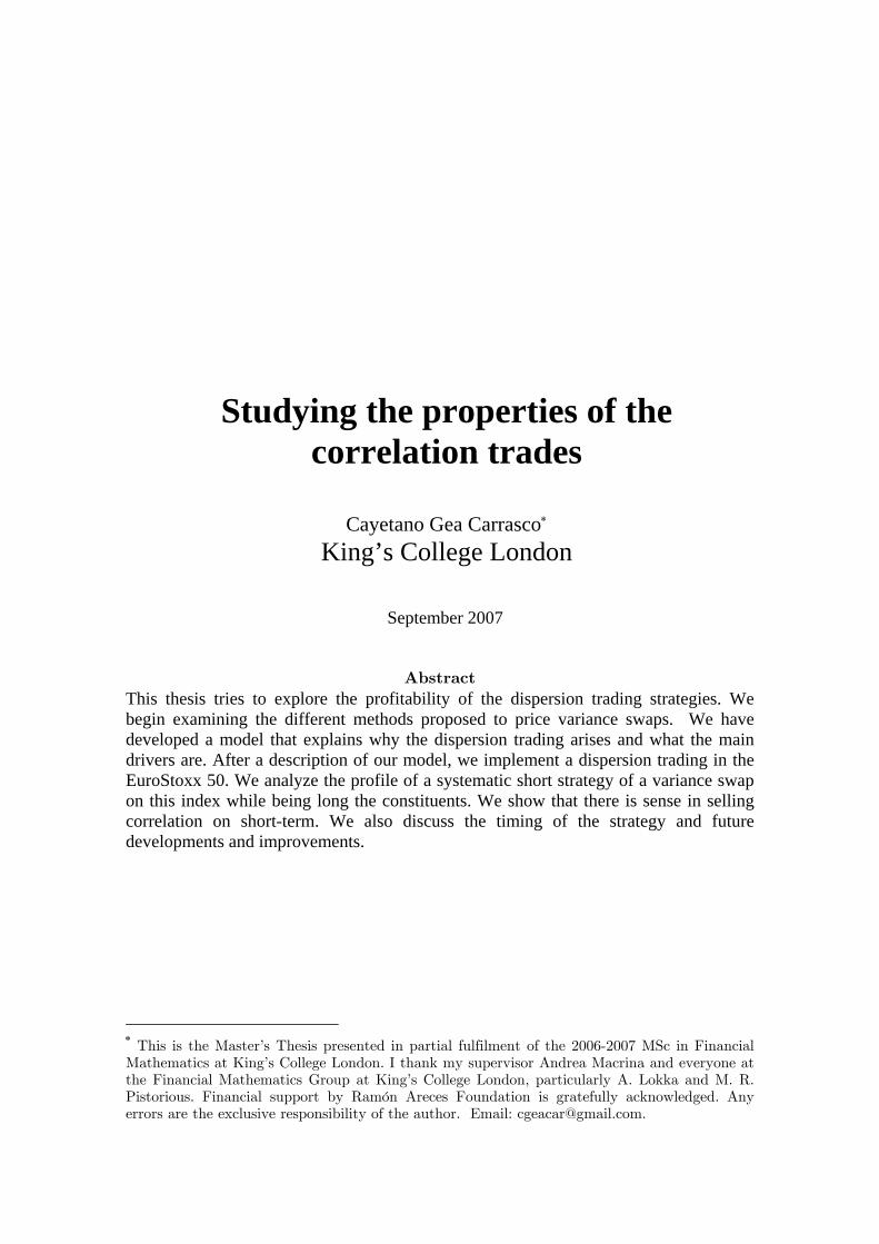
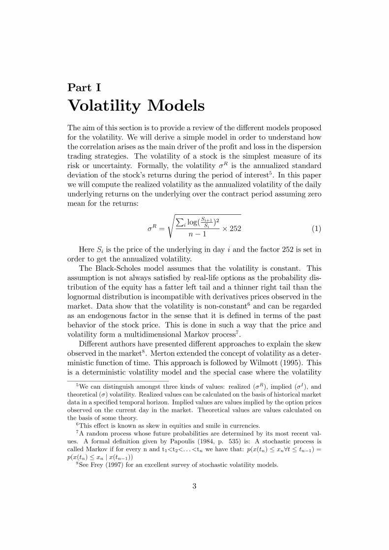
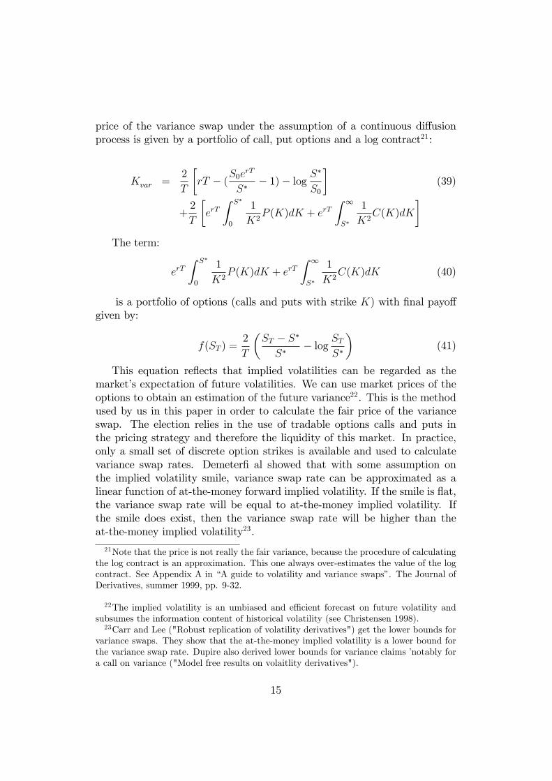
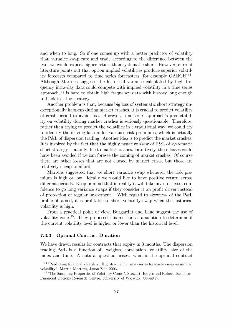
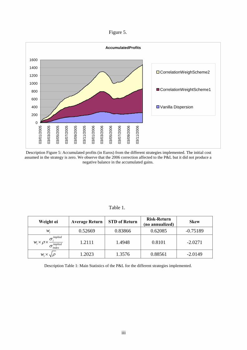
We study the performance of systematic short strategy of a variance swapon the index and being long on the constituents. The setup is that everyday we enter in a contract with expiry three months that involves sellinga variance swap on the EuroStoxx 50 and buying 50 variance swaps on theconstituents. The realized variance is as de�ned as in Part I. The transactioncost is assumed to be zero. The notional of the contracts is one (Euros). Weimplement the di¤erent weights aforementioned for both: getting volatilityexposure and getting correlation exposure. We considered the period from1 January 2005 to 8 December 2006. It is showed that the systematic shortstrategy does provide positive mean of return (3 months). However, the riskof su¤ering big losses due to large unexpected volatility in market crashes isinevitable in this strategy. Therefore, the risk of losses exists and the distrib-ution of pro�ts and losses has high skew. We compute the correlation matrixfor the P&L obtained with the di¤erent weights proposed. We observe thatthe correlation for both correlation exposure strategies (P&L) is almost iden-tical and very high (0.99). The correlation of the volatility exposure strategyversus the exposure strategy P&L is also very high (0.8). We compute thecorrelation of the P&L with the index log-returns. The value obtained is verylow for both correlation-weighted and vanilla dispersion trading (5%). Theaverage return is positive and higher for both correlation-weigthed schemesthan vanilla weighted scheme. Traditionally there was a bias for realized dis-persion to be higher than implied, but the market has gotten more and moree¢ cient and it has produced that the pro�ts obtained with the dispersiontrading are lower than historically.Table 1 at Appendix shows the main statistics of the dispersion trading

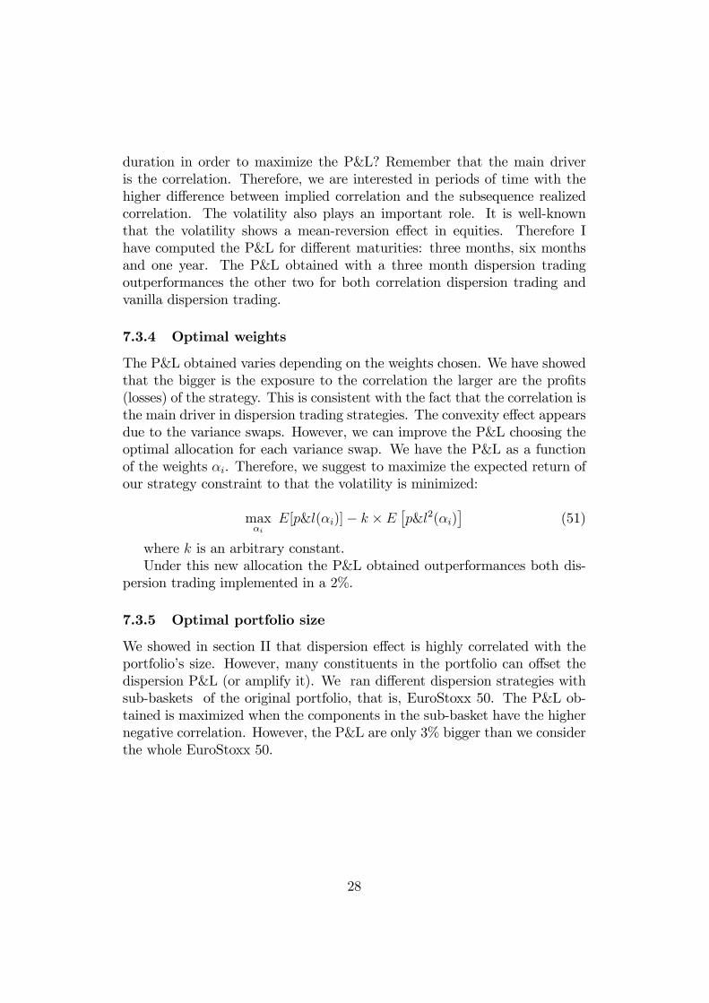
implemented for the di¤erent weights chosen. The P&L (in Vegas) for thedi¤erent weights schemes and the distribution functions are showed in Figures1, 2, 3 and 4.

24

7.3.1 Subsamples

The risk premium becomes negative mostly due to major market corrections.We can see a correction in 2005 and 2006 clearly in the P&L. The e¤ect ismore important in correlation-weighted schemes because the exposure to thecorrelation is higher than in vanilla schemes. Remember that the correlationis the main driver as we showed. On the other hand, a suddenly increased ofthe correlation if we are long in the contract also will produce bigger lossesthan vanilla.A clear example is the 2006 correction. It a¤ects to the returns accu-

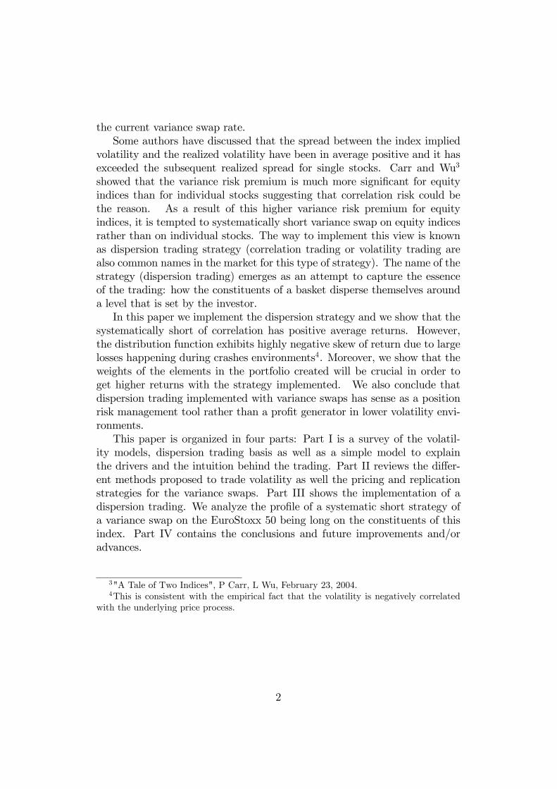
mulated during one year. However, the accumulated gains continue to bepositive while and after the crash event. The e¤ect is showed for the P&Lin Figure 5. For some investors, particularly those with short volatility posi-tions through variance swaps and dispersion trades, the increase in volatilityproduced huge losses as we can see in Figure 5.The reason of the losses was the increase in the (realized) stocks correla-

tion above the implied level (the "bet" level in the contract). The volatilityspiked in May and June a result of a pick-up in in�ation, anticipated interestrate hikes and a sell-o¤ in emerging market assets. The e¤ect is also showedby the VIX Index42. This index jumped from 13.35 points on May 16 to18.26 points on May 23. On June 13, it closed at a year high of 23.81 pointsbefore falling to 13.03 points on June 29. This is almos perfectly correlatedwith the P&L implemented (around 99.5%).The outperforming of the correlation-weighted schemes is clearly higher

than the vanilla weights. In almost all the dates the correlation weight schememakes pro�t, but between March and June in 2006 the realized volatility ofthe index was bigger than the implied (larger realized correlation than im-plied) and the P&L were negative. Think of it in a insurance term: varianceswap buyers generally pay premium to protect them against crashes (the rea-son of our positive average return), when the market crashes actually happen,variance swap seller have to pay for the claims. This also re�ects the convex-ity of the variance swaps payo¤s. This point re�ects that dispersion tradingimplemented with variance swaps can has sense as a position risk manage-ment tool rather than a pro�t generator in lower volatility environments. Ifwe want to hedge against P&L losses corresponding to volatility spikes, wecould obviously employ a variance swap or maintain an appropriate optionposition. But if we want to hedge the portfolio against a spike in correlation,an easier, although less than perfect, hedge we would try would be to �nd anasset that is signi�cantly correlated with the correlation of the index. There

42The VIX Index measures the expectation of the market of 30-day volatility on S&P500 index option prices.

25

is the risk that correlation would also break down at that time, but we wouldtest prospective candidates with a simulation. Another approach would beto study the principal components analysis in the returns of our portfolio,and use a factor model. Then we could isolate the correlation and cancelwith another asset.Therefore a �rst approximation in order to prevent the losses should be a

variance swap contract with a cap on maximum loss43. Since the systematicshort strategy is positively correlated with the return of underlying and thelosses happen mainly during market crashes, we might be able to use somevanilla instruments that can insure investors against market turndown. Wehope that they can also protect the systematic short strategy of varianceswap. Keep in mind this is not strange because the variance swap can bereplicated by a basket of put and calls with di¤erent strikes. Buying backsome options can certainly o¤set some risk of variance swap. If we buy backall the options that construct the variance swap, there will be no risk atall. However, the skew of the P&L can become positive with the help of theputs. This is because the over-the-counter put becomes pro�table in downmarket. But it is not necessarily pro�table when the variance swap contractis su¤ering a big loss.Another option can be to use barrier options. The idea to buy down-

and-in barrier put to cap the loss of variance swap comes from the intuitionthat, whenever the down-and-in put comes into existence, the underlyinghad probably been through a down and volatile period. Down-and-in barrierput is much cheaper than vanilla put of the same strike if the barrier is low.Therefore with a low barrier and a relatively high strike, a down-and-in bar-rier put option is very likely to end in-the-money for either straight downwardmarket or rebound. This captures the characteristic of being volatile.

7.3.2 Timing

As have been show in last section, systematic short strategy exhibits highlynegative skew of return due to large losses happening during market crashes.This is consistent with the empirical fact that the volatility is negativelycorrelated with the underlying price process. Thereafter it is important todetermine a timing trading strategy of variance swap. A good time to puton dispersion trade is when correlation is high.One most straight-forward idea to �nd a better forecaster of future volatil-

ity than the variance swap rate. The idea comes from that if you have per-fect foresight of future volatility then you will know perfectly when to short

43"Pricing Options on Realized Variance", P Carr, H Geman, D Madan, M Yor, August2004.

26

and when to long. So if one comes up with a better predictor of volatilitythan variance swap rate and trade according to the di¤erence between thetwo, we would expect higher return than systematic short. However, currentliterature points out that option implied volatilities produce superior volatil-ity forecasts compared to time series forecasters (for example GARCH)44.Although Martens suggests the historical variance calculated by high fre-quency intra-day data could compete with implied volatility in a time seriesapproach, it is hard to obtain high frequency data with history long enoughto back test the strategy.Another problem is that, because big loss of systematic short strategy un-

exceptionally happens during market crashes, it is crucial to predict volatilityof crash period to avoid loss. However, time-series approach�s predictabil-ity on volatility during market crashes is seriously questionable. Therefore,rather than trying to predict the volatility in a traditional way, we could tryto identify the driving factors for variance risk premiums, which is actuallythe P&L of dispersion trading. Another idea is to predict the market crashes.It is inspired by the fact that the highly negative skew of P&L of systematicshort strategy is mainly due to market crashes. Intuitively, these losses couldhave been avoided if we can foresee the coming of market crashes. Of coursethere are other losses that are not caused by market crisis, but those arerelatively cheap to a¤ord.Martens suggested that we short variance swap whenever the risk pre-

mium is high or low. Ideally we would like to have positive return acrossdi¤erent periods. Keep in mind that in reality it will take investor extra con-�dence to go long variance swaps if they consider it an pro�t driver insteadof protection of regular investment. With regard to skewness of the P&Lpro�le obtained, it is pro�table to short volatility swap when the historicalvolatility is high.From a practical point of view, Burgardht and Lane suggest the use of

volatility cones45. They proposed this method as a solution to determine ifthe current volatility level is higher or lower than the historical level.

7.3.3 Optimal Contract Duration

We have drawn results for contracts that expiry in 3 months. The dispersiontrading P&L is a function of: weights, correlation, volatility, size of theindex and time. A natural question arises: what is the optimal contract

44"Predicting �nancial volatility: High-frequency time -series forecasts vis-à-vis impliedvolatility", Martin Martens, Jason Zein 2003.45"The Sampling Properties of Volatility Cones", Stewart Hodges and Robert Tompkins.

Financial Options Research Centre, University of Warwick, Coventry.

27

duration in order to maximize the P&L? Remember that the main driveris the correlation. Therefore, we are interested in periods of time with thehigher di¤erence between implied correlation and the subsequence realizedcorrelation. The volatility also plays an important role. It is well-knownthat the volatility shows a mean-reversion e¤ect in equities. Therefore Ihave computed the P&L for di¤erent maturities: three months, six monthsand one year. The P&L obtained with a three month dispersion tradingoutperformances the other two for both correlation dispersion trading andvanilla dispersion trading.

7.3.4 Optimal weights

The P&L obtained varies depending on the weights chosen. We have showedthat the bigger is the exposure to the correlation the larger are the pro�ts(losses) of the strategy. This is consistent with the fact that the correlation isthe main driver in dispersion trading strategies. The convexity e¤ect appearsdue to the variance swaps. However, we can improve the P&L choosing theoptimal allocation for each variance swap. We have the P&L as a functionof the weights �i. Therefore, we suggest to maximize the expected return ofour strategy constraint to that the volatility is minimized:

max�i

E[p&l(�i)]� k � E�p&l2(�i)

�(51)

where k is an arbitrary constant.Under this new allocation the P&L obtained outperformances both dis-

persion trading implemented in a 2%.

7.3.5 Optimal portfolio size

We showed in section II that dispersion e¤ect is highly correlated with theportfolio�s size. However, many constituents in the portfolio can o¤set thedispersion P&L (or amplify it). We ran di¤erent dispersion strategies withsub-baskets of the original portfolio, that is, EuroStoxx 50. The P&L ob-tained is maximized when the components in the sub-basket have the highernegative correlation. However, the P&L are only 3% bigger than we considerthe whole EuroStoxx 50.

28

Part IV

Conclusions and FutureDevelopmentsThe rapid development of derivatives market has enabled investors to gainexposure to volatility. So instead of just taking directional positions basedon predictions of future returns, investor with foresight of volatilities mightalso make money by engaging in the appropriate volatility product. Varianceswap is the most heavily traded among the volatility products. The payo¤of this contract is the di¤erence between the future realized return varianceand the predetermined variance swap rate.This thesis tries to explore the pro�tability of the dispersion trading

strategies. We begin examining the di¤erent methods proposed to price vari-ance swaps. We have developed a model that explains why the dispersiontrading arises and what the main drivers are. We have investigate the P&Lobtained with the di¤erent strategies proposed in the market. We show thatcorrelation-based dispersion trading produces the bigger P&L. This strategydemonstrates positive mean of return, which is consistent with the fact thatthe implied volatility is generally higher than the future realized volatility.This strategy has a potential of su¤ering large loss in bullish market. Weshow that dispersion trading strategies are not arbitrage strategies. We havecomputed the distribution of the P&L obtained. We show that the distri-bution of the P&L shows thick tails. This is consistent with the extremeevents that appear in a bullish market (for example, the correction in themarket of 2005). We proposed a method to choose the optimal weights thatproduces outperforming of the strategies used in the market. The timing ofthe strategy is also studied.As a further it might be interesting to check the seasonality of the return

pro�le and design one optimal entry time. Furthermore, the mark to marketvalue of variance should also be studied because for long maturity contractone might prefer to close the position before maturity.We have studied the dispersion trading in a Equity Index. An interesting

exercise could be to implement the strategy in Credit Indices. This approachneeds a previous step: the modi�cation of the pricing method proposed byDerman in order to use Credit Options (in both single Credit Default Swapsand Credit Indices).

29

i

Figure 1.

P&L Dispersion Trading

-6

-5

-4

-3

-2

-1

0

1

2

3

4

03/0

1/20

05

03/0

3/20

05

03/0

5/20

05

03/0

7/20

05

03/0

9/20

05

03/1

1/20

05

03/0

1/20

06

03/0

3/20

06

03/0

5/20

06

03/0

7/20

06

03/0

9/20

06

03/1

1/20

06Date

Vanilla Dispersion

Correlation WeightedScheme 1

Correlation WeightedScheme 2

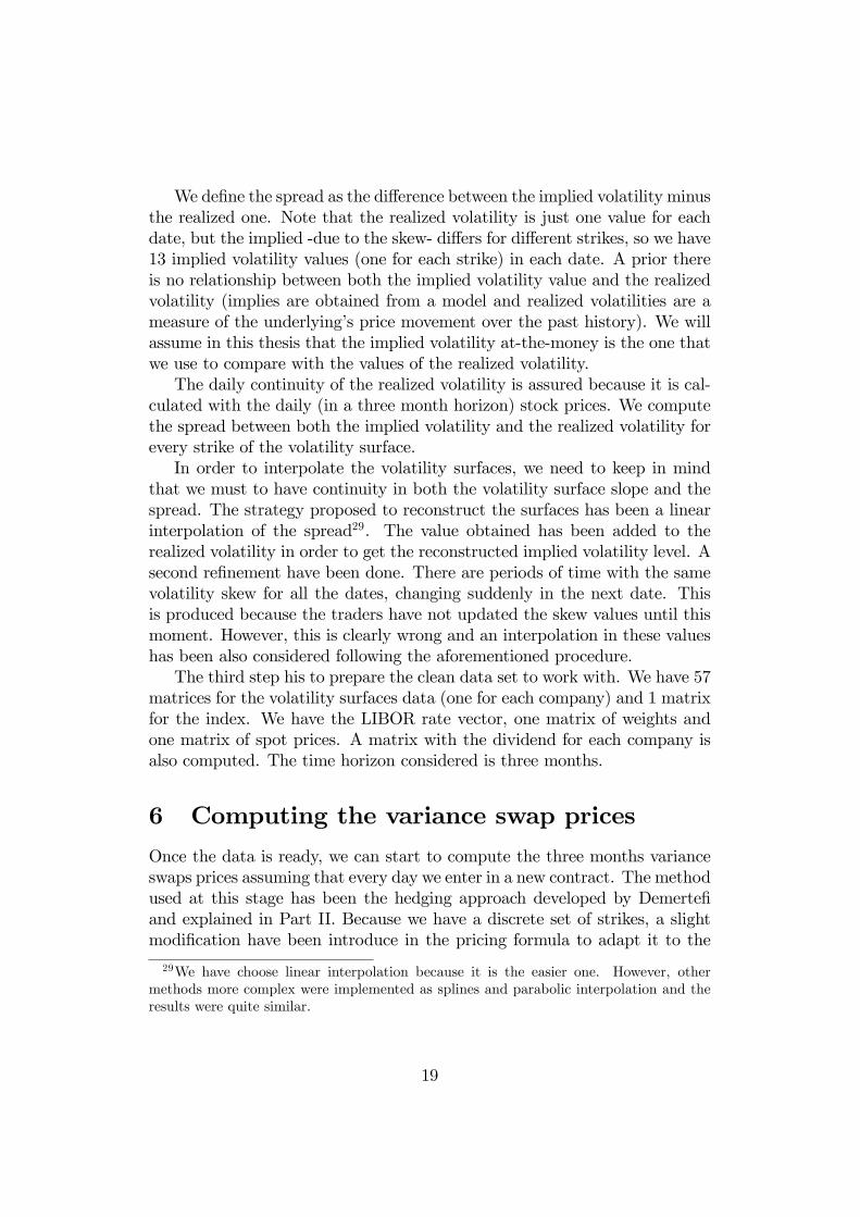
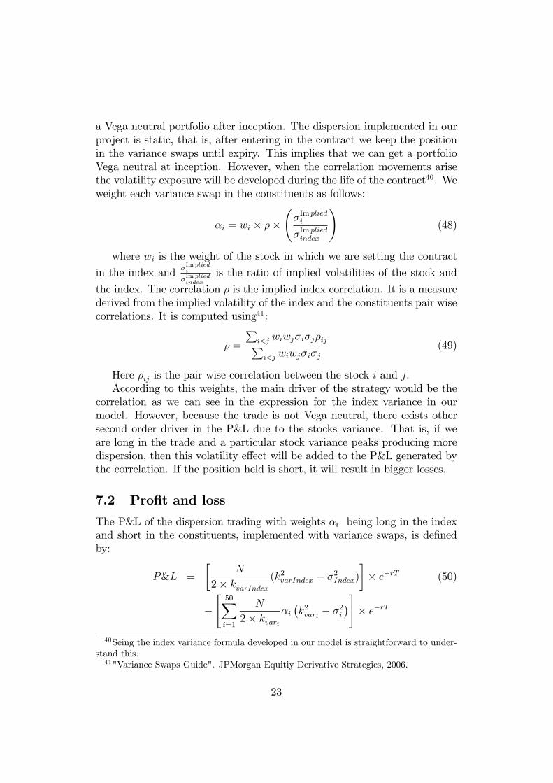
Description Figure 1: P&L (in Vega Notional) obtained selling a variance swap on the EuroStoxx 50 and being long on the constituents. Vanilla dispersion gets exposure to the volatility and correlation-weighted

dispersion gets exposure to the correlation. The expiry is three months and the Notional is one Euro. Figure 2.

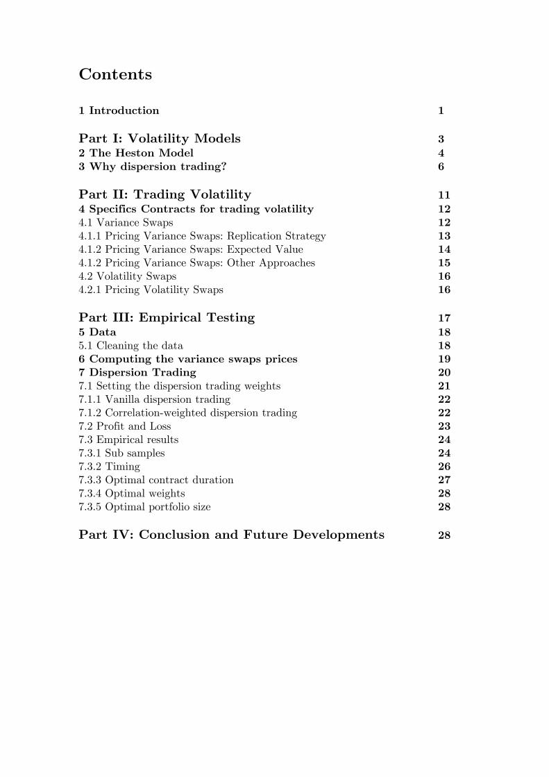
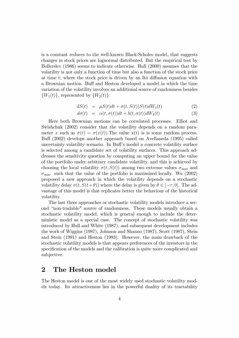
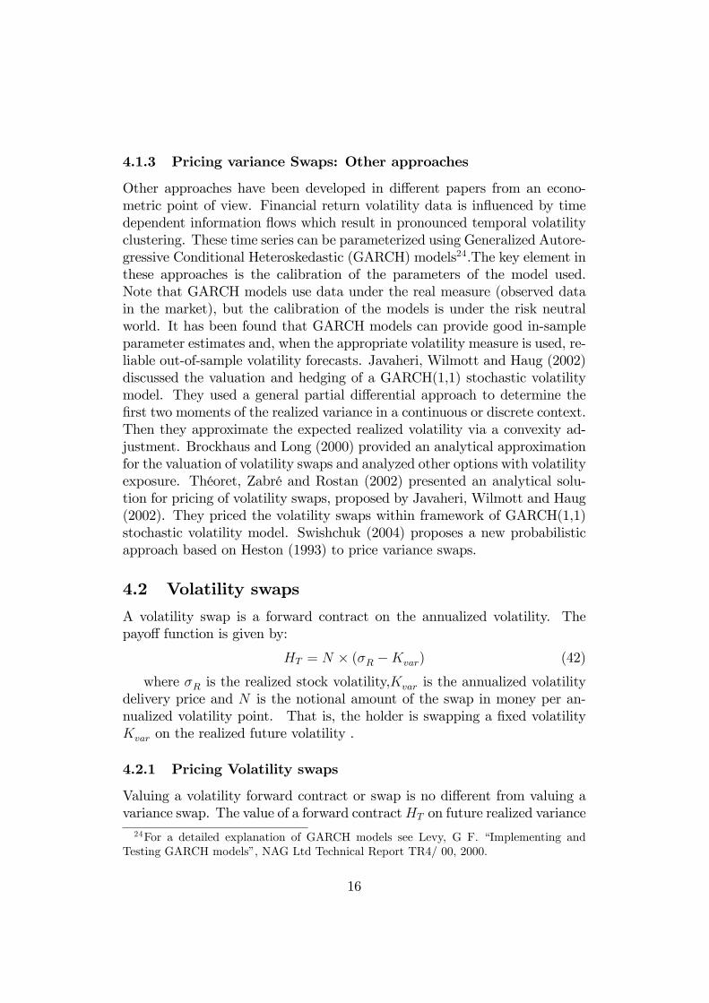
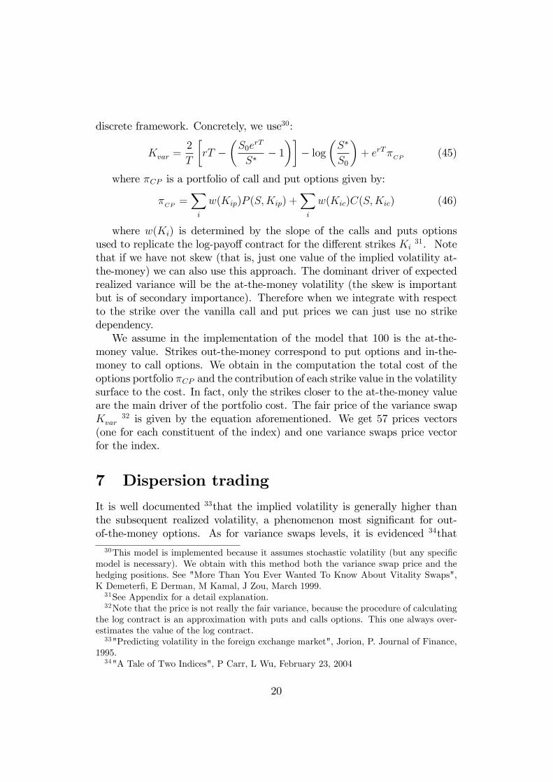
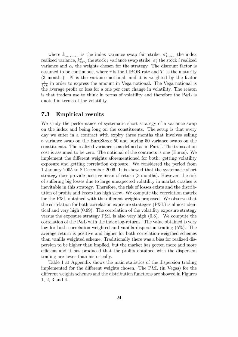
Description Figure 2: Distribution function obtained for the Vanilla Dispersion Trading on the EuroStoxx 50.

The weight used is wi.

-0.5 0 0.5 1 1.5 2 2.50

2

4

6

8

10

12Vanilla Dispersion Distribution Function

ii

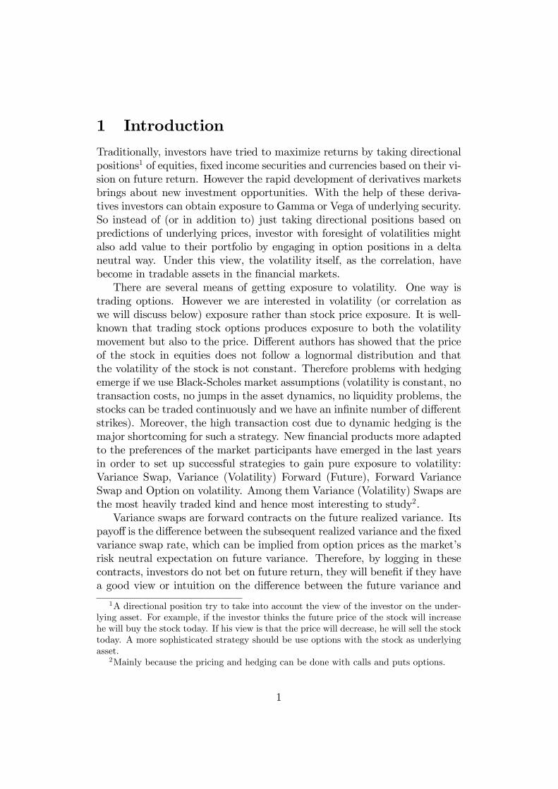
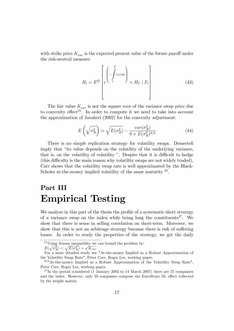
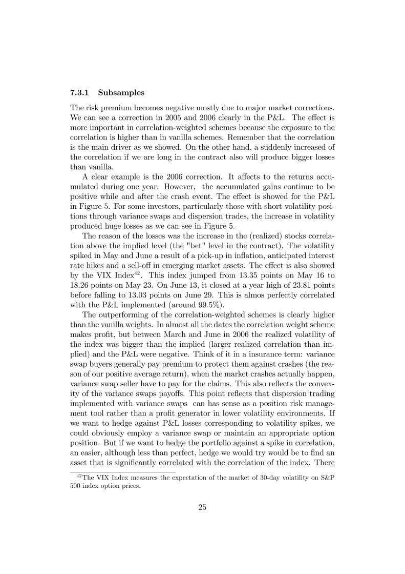
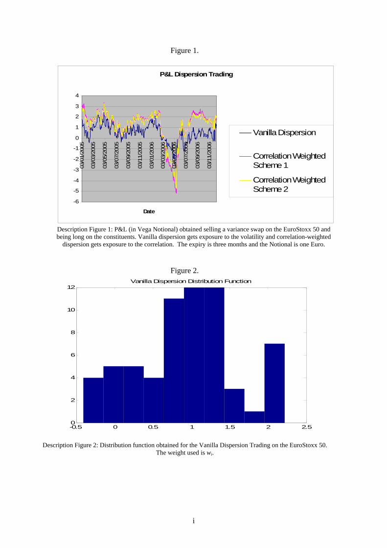
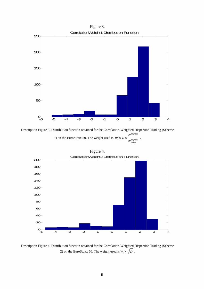
Figure 3.

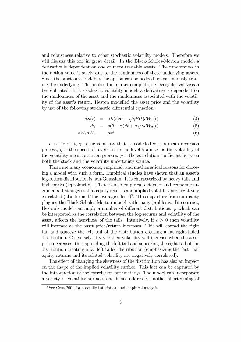
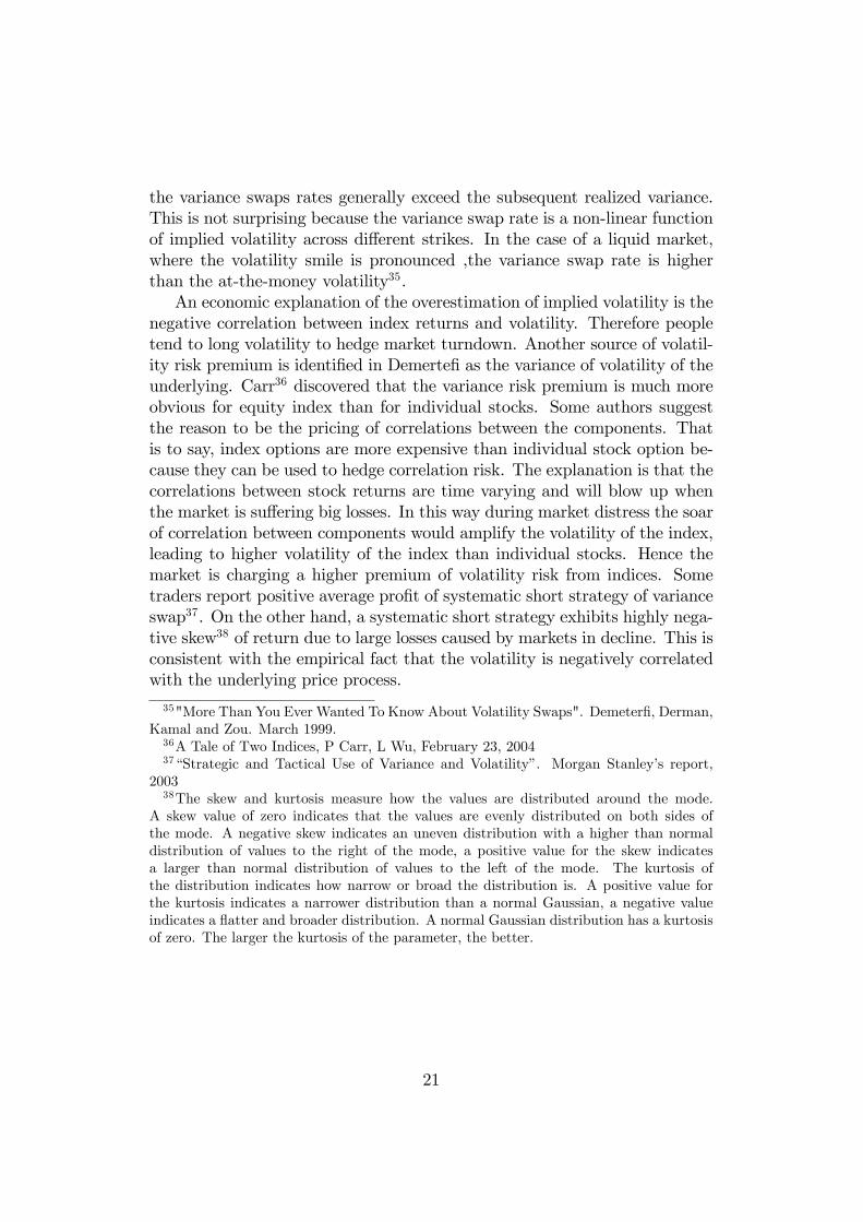
Description Figure 3: Distribution function obtained for the Correlation-Weighted Dispersion Trading (Scheme

1) on the EuroStoxx 50. The weight used is impliedi

i impliedindex

w σρσ

× × .

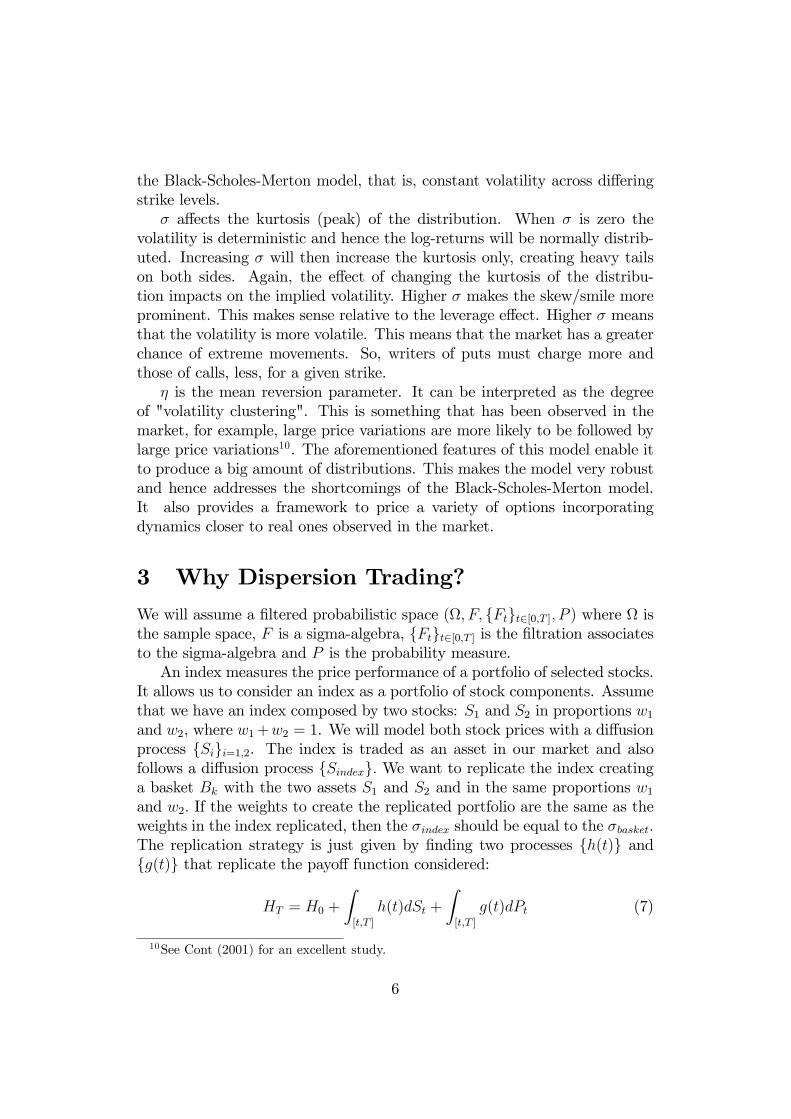
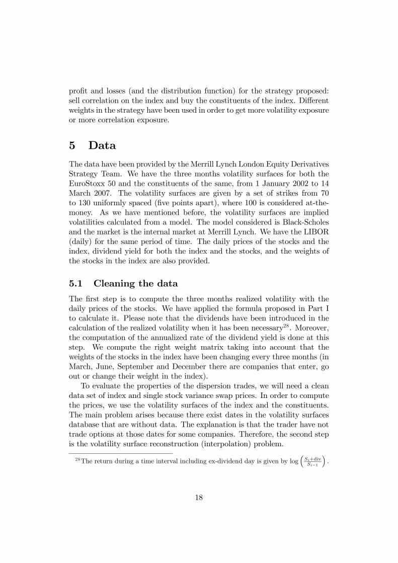
Figure 4.

Description Figure 4: Distribution function obtained for the Correlation-Weighted Dispersion Trading (Scheme

2) on the EuroStoxx 50. The weight used is iw ρ× .

-5 -4 -3 -2 -1 0 1 2 3 40

20

40

60

80

100

120

140

160

180

200CorrelationWeight2 Distribution Function

-6 -5 -4 -3 -2 -1 0 1 2 3 40

50

100

150

200

250CorrelationWeight1 Distribution Function

iii

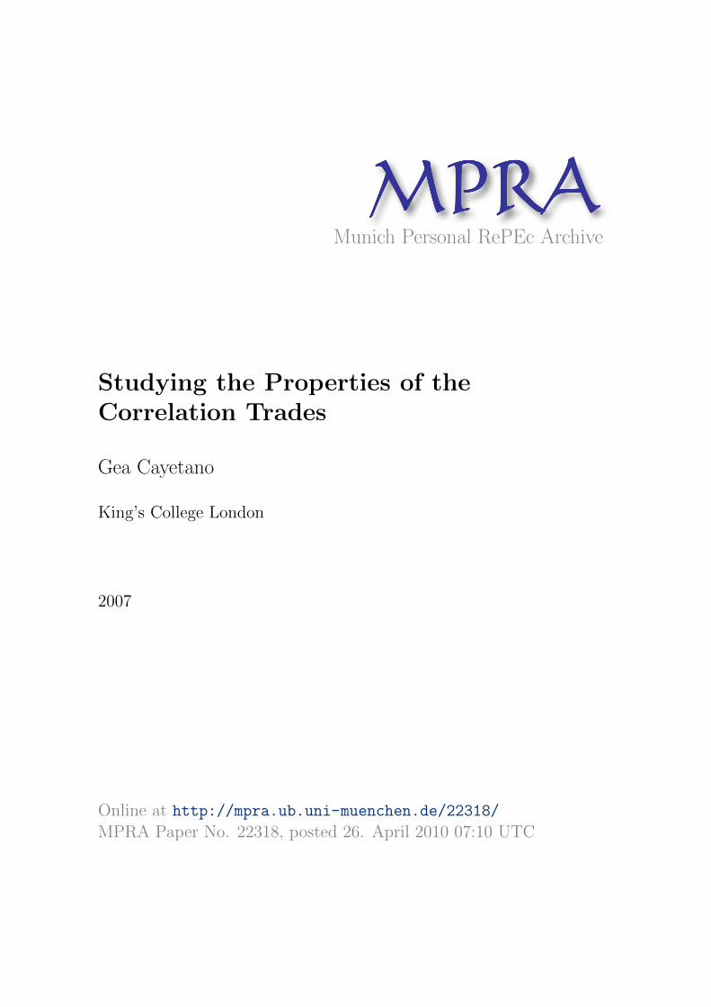
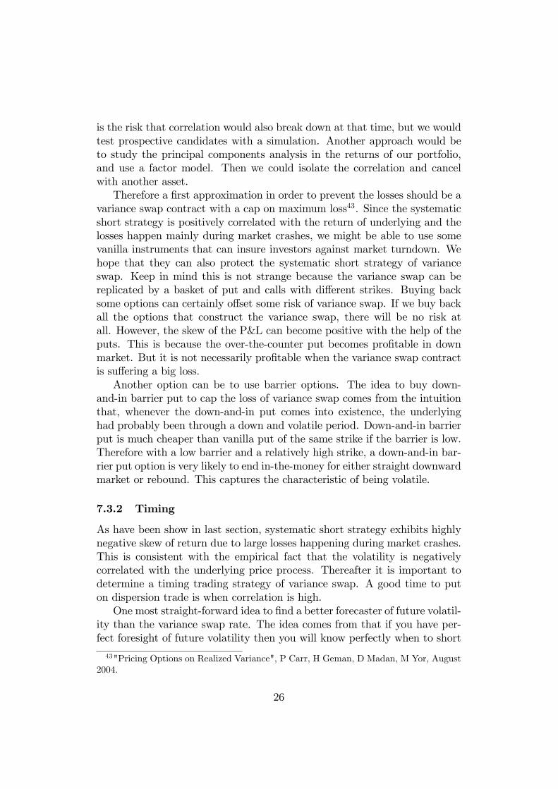
Figure 5.

AccumulatedProfits

0

200

400

600

800

1000

1200

1400

1600

03/0

1/20

05

03/0

3/20

05

03/0

5/20

05

03/0

7/20

05

03/0

9/20

05

03/1

1/20

05

03/0

1/20

06

03/0

3/20

06

03/0

5/20

06

03/0

7/20

06

03/0

9/20

06

03/1

1/20

06

CorrelationWeighScheme2

CorrelationWeightScheme1

Vanilla Dispersion

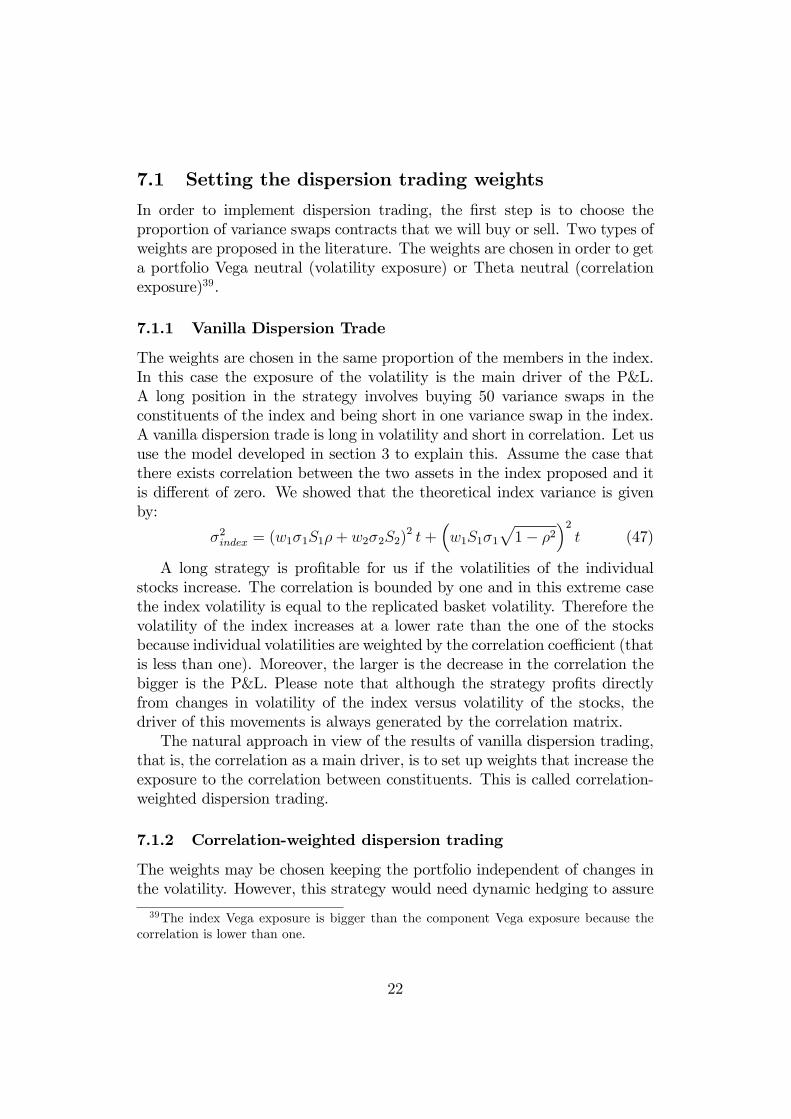
Description Figure 5: Accumulated profits (in Euros) from the different strategies implemented. The initial cost assumed in the strategy is zero. We observe that the 2006 correction affected to the P&L but it did not produce a

negative balance in the accumulated gains. Table 1.

Weight αi Average Return STD of Return Risk-Return (no annualized) Skew

iw 0.52669 0.83866 0.62085 -0.75189 impliedi

i impliedindex

w σρσ

× × 1.2111 1.4948 0.8101 -2.0271

iw ρ× 1.2023 1.3576 0.88561 -2.0149

Description Table 1: Main Statistics of the P&L for the different strategies implemented.

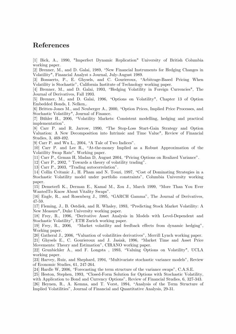
References [1] Bick, A., 1990, "Imperfect Dynamic Replication" University of British Columbia working paper. [2] Brenner, M., and D. Galai, 1989, “New Financial Instruments for Hedging Changes in Volatility", Financial Analyst's Journal, July-August 1989. [3] Bossaerts, P., E. Ghysels, and C. Gourieroux, “Arbitrage-Based Pricing When Volatility is Stochastic”, California Institute of Technology working paper. [4] Brenner, M., and D. Galai, 1993, “Hedging Volatility in Foreign Currencies", The Journal of Derivatives, Fall 1993. [5] Brenner, M., and D. Galai, 1996, “Options on Volatility", Chapter 13 of Option Embedded Bonds, I. Nelken,. [6] Britten-Jones M., and Neuberger A., 2000, “Option Prices, Implied Price Processes, and Stochastic Volatility", Journal of Finance. [7] Bühler H., 2006, “Volatility Markets: Consistent modelling, hedging and practical implementation”. [8] Carr P. and R. Jarrow, 1990, “The Stop-Loss Start-Gain Strategy and Option Valuation: A New Decomposition into Intrinsic and Time Value", Review of Financial Studies, 3, 469-492. [9] Carr P. and Wu L., 2004, “A Tale of Two Indices”. [10] Carr P. and Lee R., “At-the-money Implied as a Robust Approximation of the Volatility Swap Rate”. Working paper. [11] Carr P., Geman H, Madan D, August 2004, “Pricing Options on Realized Variance”. [12] Carr P., 2002, ” Towards a theory of volatility trading”. [13] Carr P., 2003, “Trading autocorrelation”. [14] Collin Cvitanic J., H. Pham and N. Touzi, 1997, “Cost of Dominating Strategies in a Stochastic Volatility model under portfolio constraints”, Columbia University working paper. [15] Demeterfi K., Derman E., Kamal M., Zou J., March 1999, “More Than You Ever WantedTo Know About Vitality Swaps”. [16] Engle, R., and Rosenberg J., 1995, “GARCH Gamma”, The Journal of Derivatives, 47-59. [17] Fleming, J., B. Ostdiek, and R. Whaley, 1993, “Predicting Stock Market Volatility: A New Measure", Duke University working paper. [18] Frey, R., 1996, “Derivative Asset Analysis in Models with Level-Dependent and Stochastic Volatility”, ETH Zurich working paper. [19] Frey, R., 2006, “Market volatility and feedback effects from dynamic hedging”, Working paper. [20] Gatheral J., 2006, “Valuation of volatilities derivatives”, Merrill Lynch working paper. [21] Ghysels E., C. Gourieroux and J. Jasiak, 1996, “Market Time and Asset Price Movements: Theory and Estimation”, CIRANO working paper. [22] Grunbichler A., and F. Longsta , 1993, “Valuing Options on Volatility", UCLA working paper. [23] Harvey, Ruiz, and Shephard, 1994, “Multivariate stochastic variance models”, Review of Economic Studies, 61, 247-264. [24] Hardle W, 2006, “Forecasting the term structure of the variance swaps”, C.A.S.E. [25] Heston, Stephen, 1993, “Closed-Form Solution for Options with Stochastic Volatility, with Application to Bond and Currency Options”, Review of Financial Studies, 6, 327-343. [26] Heynen, R., A. Kemna, and T. Vorst, 1994, “Analysis of the Term Structure of Implied Volatilities”, Journal of Financial and Quantitative Analysis, 29-31.

[27] Heston, S, 1997, “Garch option pricing model”, Working paper. [28] JP Morgan, 2006, “Variance Swaps guide”. [29] Martens M., Zein J, 2003, “Predicting financial volatility: High-frequency time -series forecasts vis-à-vis implied volatility”. Working paper. [30] Prabhala, “N.R The relation between implied and realized volatility”. Journal of Financial Economics(1998) [31] Swishchuk A., 2006, “Modelling and Pricing of Variance Swaps for Stochastic Volatilities with Delay”. [32] Vetzal R., 2003, “Pricing methods for volatility derivatives”.