Embed Size (px)
Citation preview

Universita degli Studi di Pisa
Master’s Degree in Mathematics
Volatility and Dispersionstrategies in Finance
Master’s Thesis
CandidateFederico Borghese
SupervisorMaurizio PratelliUniversita di Pisa
SupervisorAntoine Garaıalde
J.P. Morgan
Anno Accademico 2015/2016
October 14, 2016


Universita degli Studi di Pisa
Master’s Degree in Mathematics
Volatility and Dispersionstrategies in Finance
CandidateFederico Borghese1
SupervisorMaurizio PratelliUniversita di Pisa
SupervisorAntoine Garaıalde
J.P. Morgan
October 14, 2016
1Equity Derivatives Structuring at J.P. Morgan - Universita di Pisa - Scuola NormaleSuperiore - M2 Probabilites et Finance (Paris 6 & Ecole Polytechnique).Contact: [email protected]

Contents
1 J.P. Morgan Equity Derivatives Structuring Group 81.1 J.P. Morgan . . . . . . . . . . . . . . . . . . . . . . . . . . . . 81.2 Equity Derivatives Structuring . . . . . . . . . . . . . . . . . . 8
1.2.1 A bridge between Trading and Sales . . . . . . . . . . 9
2 Preparatory concepts 112.1 European Payoff replication with vanilla options . . . . . . . . 11
2.1.1 Proof . . . . . . . . . . . . . . . . . . . . . . . . . . . . 122.2 Ito-Tanaka’s formula . . . . . . . . . . . . . . . . . . . . . . . 132.3 Gamma P&L . . . . . . . . . . . . . . . . . . . . . . . . . . . 142.4 Basket of n stocks . . . . . . . . . . . . . . . . . . . . . . . . . 15
3 Volatility products 193.1 Introduction . . . . . . . . . . . . . . . . . . . . . . . . . . . . 19
3.1.1 Implied Volatility . . . . . . . . . . . . . . . . . . . . . 203.1.2 Realized Volatility . . . . . . . . . . . . . . . . . . . . 20
Realised volatility in a stochastic volatility model . . . 223.2 Variance Swaps . . . . . . . . . . . . . . . . . . . . . . . . . . 22
3.2.1 Replication and fair strike of a Variance Swap . . . . . 233.2.2 Sensitivities . . . . . . . . . . . . . . . . . . . . . . . . 24
Vega . . . . . . . . . . . . . . . . . . . . . . . . . . . . 25Delta . . . . . . . . . . . . . . . . . . . . . . . . . . . . 26Gamma . . . . . . . . . . . . . . . . . . . . . . . . . . 26Theta . . . . . . . . . . . . . . . . . . . . . . . . . . . 26Vanna . . . . . . . . . . . . . . . . . . . . . . . . . . . 27
3.2.3 Derivation of the replication in a stochastic volatilitymodel . . . . . . . . . . . . . . . . . . . . . . . . . . . 27The realized variance is the sum of a delta strategy and
a log contract . . . . . . . . . . . . . . . . . . 27The log contract can be replicated with a strip of vanilla
Calls and Puts . . . . . . . . . . . . . . . . . 28
5

Federico Borghese Volatility and Dispersion strategies in Finance
3.3 Variations of Variance Swaps . . . . . . . . . . . . . . . . . . . 283.3.1 Corridor Variance Swaps Definitions . . . . . . . . . . 283.3.2 Up Variance Replication . . . . . . . . . . . . . . . . . 303.3.3 Weighted Variance Swap replication . . . . . . . . . . . 323.3.4 Gamma Swaps . . . . . . . . . . . . . . . . . . . . . . 33
Weighted additivity property for Gamma Swaps . . . . 34Sensitivities . . . . . . . . . . . . . . . . . . . . . . . . 35
3.3.5 Corridor Variance Swap Replication . . . . . . . . . . . 373.3.6 Re-finding the Variance Swap . . . . . . . . . . . . . . 373.3.7 Volatility Swaps . . . . . . . . . . . . . . . . . . . . . . 37
Strike of a Volatility Swap . . . . . . . . . . . . . . . . 383.4 Backtest . . . . . . . . . . . . . . . . . . . . . . . . . . . . . . 38
3.4.1 Replication with 4 options, step 10% . . . . . . . . . . 403.4.2 Replication with 8 options, step 5% . . . . . . . . . . . 413.4.3 Replication with 6 options, step 25% . . . . . . . . . . 423.4.4 Replication with 8 options, step 10% . . . . . . . . . . 433.4.5 Replication with 18 options, step 5% . . . . . . . . . . 44
4 Correlation 454.1 Different types of correlations . . . . . . . . . . . . . . . . . . 45
4.1.1 Pearson Correlation . . . . . . . . . . . . . . . . . . . . 454.1.2 Kendall and Spearman Correlation . . . . . . . . . . . 47
Spearman Correlation . . . . . . . . . . . . . . . . . . 47Kendall Correlation . . . . . . . . . . . . . . . . . . . . 47Relationship with Pearson correlation for Gaussian vec-
tors . . . . . . . . . . . . . . . . . . . . . . . 48Example: spot/div correlation . . . . . . . . . . . . . . 49
4.1.3 Correlation in the Black-Scholes model . . . . . . . . . 514.1.4 Realised correlation and Picking Frequency . . . . . . . 52
The Picking Frequency correlation still estimates cor-relation . . . . . . . . . . . . . . . . . . . . . 53
Why using Picking Frequencies . . . . . . . . . . . . . 534.2 Correlation of n > 2 assets . . . . . . . . . . . . . . . . . . . . 55
4.2.1 Average Pairwise Correlation . . . . . . . . . . . . . . 564.2.2 Clean and Dirty Correlations . . . . . . . . . . . . . . 56
Realized volatility of the basket . . . . . . . . . . . . . 58
5 Dispersion 595.1 Interest in trading correlation . . . . . . . . . . . . . . . . . . 595.2 General Dispersion Trade . . . . . . . . . . . . . . . . . . . . . 605.3 Gamma P&L . . . . . . . . . . . . . . . . . . . . . . . . . . . 61
6

Federico Borghese Volatility and Dispersion strategies in Finance
5.4 Examples of Dispersion Strategies . . . . . . . . . . . . . . . . 635.4.1 Variance Swap VS Variance Swap Dispersion . . . . . . 63
Weightings . . . . . . . . . . . . . . . . . . . . . . . . . 645.4.2 Synthetic Variance Swap Dispersion . . . . . . . . . . . 655.4.3 ATM Call VS Call Dispersion . . . . . . . . . . . . . . 665.4.4 Straddle VS Straddle or Put VS Put . . . . . . . . . . 675.4.5 Call Strip VS Call Strip . . . . . . . . . . . . . . . . . 67
5.5 Backtest . . . . . . . . . . . . . . . . . . . . . . . . . . . . . . 68
6 Some new ideas 706.1 Putting together Dispersion and Variance Replication: The
Gamma Covariance Swap . . . . . . . . . . . . . . . . . . . . 706.1.1 Replication . . . . . . . . . . . . . . . . . . . . . . . . 716.1.2 Backtest . . . . . . . . . . . . . . . . . . . . . . . . . . 73
6.2 The FX-Gamma Covariance . . . . . . . . . . . . . . . . . . . 776.2.1 Replication . . . . . . . . . . . . . . . . . . . . . . . . 776.2.2 The FX-Gamma Covariance as a form of Quanto For-
ward Delta Hedged and FX Hedged . . . . . . . . . . . 786.2.3 Conclusions . . . . . . . . . . . . . . . . . . . . . . . . 79
Conclusions 80
Acknowledgements 82
Bibliography 84
7

Chapter 1
J.P. Morgan Equity DerivativesStructuring Group
1.1 J.P. Morgan
J.P. Morgan is one of the most respected financial services firms in the world,serving governments, corporations and institutions in over 100 countries. Thefirm is a leader in investment banking, financial services for consumers andsmall businesses, commercial banking, financial transaction processing andasset management.With a history dating back over 200 years, J.P. Morgan is one of the oldestfinancial institutions in the United States. It is the largest bank in the US,and the world’s sixth largest bank by total assets, with total assets of US$2.4trillion. It employs more than 235, 000 people worldwide.The Firm and its Foundation give approximately $200 million annually tonon-profit organizations around the world. J.P. Morgan also leads volunteerservice activities for employees in local communities.
1.2 Equity Derivatives Structuring
Equity Derivatives Structuring focuses on developing alternative payoff pro-files for a wide range of investors, running from highly sophisticated insti-tutional investors (Hedge Funds, Asset Managers, Pension Funds, InsuranceCompanies) to less sophisticated ones (Retail). The Team designs and pricesboth new and existing structured products in the core equity derivativesspace. There is no precise definition of what alternative payoffs are; every-thing which is not a easily accessed by vanilla options and futures on commonasset classes can be regarded as an alternative payoff.
8

Federico Borghese Volatility and Dispersion strategies in Finance
The product offering is very wide. It includes new derivative ideas inspiredfrom research, existing derivatives and fully tailored solutions for the clientswhich are designed according to their return expectations, their risk appetiteand their views on the market. For example, the Team offers sophisticatedinstitutional investors ideas to trade volatility, correlation and skew.The business has considerably changed after the 2008 financial crisis. Theregulator is not in favour of complexity and the range of the products hassignificantly shrunk. However, the range of possible underlyings has consider-ably widened and the interest from clients stays strong. J.P. Morgan developsproprietary indices which implement systematic strategies on which simplederivative products can be written, achieving simplicity and innovation atthe same time.
1.2.1 A bridge between Trading and Sales
Equity Derivatives Structurers have the important task to price their prod-ucts. The Black-Scholes model and its variations, which are widely usedfor pricing structured products, can’t keep in consideration all the possiblefactors influencing the market evolution. For example,
• Volatility is not deterministic, but stochastic. The market is not com-plete, i.e. it is not possible to perfectly replicate derivatives using theunderlying only.
• The are jumps in the spot price evolution. Often these jumps are dueto news such as macroeconomics news, central bank policy, politicalnews, release of a new product, quarterly reports etc. Jumps are highlyunpredictable and always set big challenges to hedging.
• There are transaction costs to trading the underlying and there is abid-offer spread.
• Not every underlying and vanilla option is available in the market.
Structurers’ skills include determining these extra-model risks and incorpo-rate them in the price.The products are sold by Sales people, who always need the lowest possibleprice to beat the competition and secure the trade with the client. After thesale, the Trading Desk has to hedge the product in order to neutralize thebank’s position and avoid any losses. Therefore the Trading Desk wants toincorporate in the price all the possible hedging risks. The goal of the pricecomputed by the Structuring Desk is to make a good compromise betweenSales and Trading.
9

Federico Borghese Volatility and Dispersion strategies in Finance
Moreover, in the product development process, the Structuring Desk needsto know both the Sales and the Trading points of view. They need to knowthe clients, the type of products which are popular in the market, they haveto find attractive payoffs and underlyings that can be advertised. But theyalso have to think about the hedging strategies, the potential sources of risk,the sensitivities, the status of the traders’ books.
10

Chapter 2
Preparatory concepts
This brief chapter recalls a few mathematical tools that will be used through-out this document. We don’t report the basics of mathematical finance,which can be found in [2] and [3].
2.1 European Payoff replication with vanilla
options
This result is sometimes known as Carr’s formula. Let G : R+ → R atwice differentiable function (can be relaxed to G being the difference oftwo convex functions or even more than that). Consider a contract on anunderlying S which pays at maturity T the amount G(ST ). This is whatis called a European payoff: the final value of the contract depends only onthe final price of the underlying, and the contract cannot be unwound beforematurity.Suppose we have a liquid market of Call and Put Options on the underlyingwith the same maturity T , with quoted prices Call(K) for every strike K ≥S∗ and Put(K) for every strike K ≤ S∗.Then we can perfectly replicate the European Payoff G(ST ) using only azero-coupon bond, a forward contract on the underlying and the Calls andPuts in the following manner:
G(ST ) = G(S∗) +G′(S∗)(ST − S∗)+
+
∫ S∗
0
G′′(K)(K − ST )+dK +
∫ ∞S∗
G′′(K)(ST −K)+dK(2.1)
11
Federico Borghese Volatility and Dispersion strategies in Finance
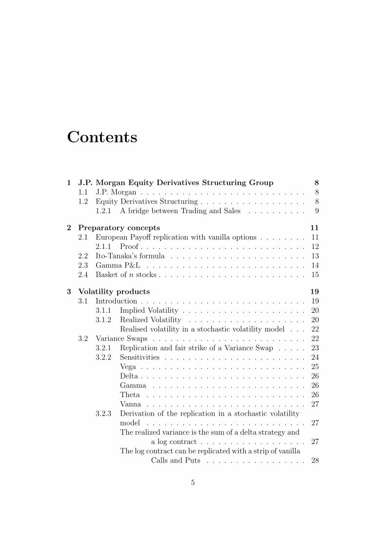
As a consequence, the only allowable price for the contract in order to preventany arbitrage is
Contract price = G(S∗)B(0, T ) +G′(S∗)(price of a forward struck at S∗)+
+
∫ S∗
0
G”(K)Put(K)dK +
∫ ∞S∗
G”(K)Call(K)dK
(2.2)
where B(0, T ) is the price of a zero-coupon bond with maturity T .
2.1.1 Proof
Proof. Assume that G is twice differentiable1. By the integration by partsformula, we have∫ +∞
S∗G”(K)(x−K)+dK = [G′(K)(x−K)+]
+∞S∗ +
∫ +∞
S∗G′(K)1{x≥K}dK∫ S∗
0
G”(K)(K − x)+dK = [G′(K)(K − x)+]S∗
0 −∫ S∗
0
G′(K)1{x≤K}dK
(2.3)
The terms in brackets evaluated at K = 0 and K = +∞ are equal to zero,so we can rewrite∫ +∞
S∗G”(K)(x−K)+dK = −G′(S∗)(x− S∗)+ + (G(x ∨ S∗)−G(S∗))∫ S∗
0
G”(K)(K − x)+dK = G′(S∗)(S∗ − x)+ − (G(S∗)−G(x ∧ S∗))
(2.4)
By summing the previous two equations, we get:∫ S∗
0
G”(K)(K − x)+dK +
∫ +∞
S∗G”(K)(x−K)+dK =
= G′(S∗)(S∗ − x)−G(S∗) +G(x)
(2.5)
Reordering the terms and evaluating at x = ST we find back equation (2.1).
1The proof is the same in the case of G being the difference of convex functions. Inthis case G has a left derivative and its second derivative in the sense of distributions (aRadon measure) satisfies the integration by parts by definition.
12

Federico Borghese Volatility and Dispersion strategies in Finance
2.2 Ito-Tanaka’s formula
Ito’s formula, one of the most useful tools in mathematical finance, is onlyvalid for C2 functions. In the market, however, we very often deal withfunctions which are not twice differentiable. Even the simplest derivativeproduct, a Call Option, has a payoff which is not C2.This regularity hypothesis is very often neglected by practitioners, becausein many cases a “cheating” Ito’s formula provides the good result. In thissection we provide rigorous theorems which allow us to deal with functionsbelonging to a wider regularity class. Ito-Tanaka’s formula can be applied toall functions which are difference of convex functions.
Let f : R→ R a convex function, and let f ′− be its left derivative. Beingf convex, the second derivative f” in the sense of distributions is a positiveRadon measure. Let (Xt) be a continuous semimartingale with quadraticvariation [X,X]t and take a ∈ R; we define a stochastic process (Lat )t≥0, theLocal Time of X at a:
Lat = limε↘0
1
ε
∫ t
0
1[a,a+ε)(Xs)d[X,X]s
The Local Time is an increasing, non-negative process, null at 0. Lat canbe thought as the time spent by the semimartingale at point a in the timeperiod [0, t], measured in the natural time scale of the semimartingale. Forfurther details see [1].
Theorem 2.1. (Ito-Tanaka’s formula) Take f : R→ R convex and (Xt)t∈[0,T ]
a continuous semimartingale. Then
f(Xt)− f(X0) =
∫ t
0
f ′−(Xs)dXs +1
2
∫RLat f”(da)
where Lat is the Local Time of the semimartingale and f”(da) is the Radonmeasure associated with the second derivative of f .
In many cases in finance, the measure f” is absolutely continuous withrespect to Lebesgue measure. In this simpler case, we can use the OccupationTimes Formula to handle the Local Time term in the previous formula:
Theorem 2.2. (Occupation Times) Take (Xt) a semimartingale. Almostsurely, ∀T > 0 and for all F : R→ R positive Borelian function,∫ +∞
−∞LatF (a)da =
∫ T
0
F (Xs)d[X,X]s
where [X,X]s is the quadratic variation of the semimartingale.
13

Federico Borghese Volatility and Dispersion strategies in Finance
Being the two previous formulas linear in f , obviously they can beextended to all the functions that can be written as a difference of convexfunction. Combining the two formulas we can state the following extendedIto’s Formula:
Theorem 2.3. Let (Xt)t∈[0,T ] be a continuous semimartingale. Letf : R → R be the difference of two convex functions. Assume that thesecond derivative of f (which is a signed Radon measure) is absolutelycontinuous with respect to Lebesgue measure, with its Radon-Nikodymderivative denoted f”(x). Then
f(Xt)− f(X0) =
∫ t
0
f ′−(Xs)dXs +1
2
∫ t
0
f”(Xs)d[X,X]s (2.6)
2.3 Gamma P&L
When an investment bank sells a derivative product, its trading desk usuallyDelta-Hedges it. Therefore, what really matters for the P&L of the bank isnot the payoff of the product itself, but the P&L of the Delta-Hedged product.Let g(ST ) be an European payoff on the underlying St, with vt = v(t, St)being the fair price of the product at time t. The Theta, Delta and Gammaof the product are
θt =∂v(t, x)
∂t(x = St) ; δt =
∂v(t, x)
∂x(x = St) ; Γt =
∂2v(t, x)
∂x2(x = St)
(2.7)Assume for simplicity the existence of a risk-free rate r. The Delta-Hedgeportfolio Vt is a self-financed portfolio with V0 = v0 equal to the optionpremium and
dVt = δtdSt + (Vt − δtSt)rdt (2.8)
Let us work in the Black-Scholes framework, where
dStSt
= rdt+ σdWt (2.9)
where W is a Brownian Motion under the risk-neutral measure. The positionof the trader having sold the product is then Vt − vt.By Black-Scholes equation, we have
θt + rStδt +1
2Γtσ
2S2t − rv = 0 (2.10)
14

Federico Borghese Volatility and Dispersion strategies in Finance
Let ∆t be a short time period, say one day. Over this period, by Taylorexpansion on v, the changes in the option value is
∆v ≈ θ∆t+ δ∆S +1
2Γ(∆S)2 (2.11)
By equation (2.10), we have
∆V = δ∆S + (V − δS)r∆t =
= δ∆S + (v − δS)r∆t+ (V − v)r∆t =
= δ∆S +
(θ +
1
2Γσ2S2
)∆t+ (V − v)r∆t
(2.12)
Combining the previous equations we find the total daily Gamma P&L ofthe trader:
P&LΓ = ∆(Vt − vt) ≈1
2ΓtS
2t
[σ2∆t−
(∆StSt
)2]
+ (V − v)r∆t (2.13)
The previous equation can be interpreted in terms of the discounted P&L:
discounted P&LΓ = ∆(e−rt(Vt − vt)
)≈ e−rt
1
2ΓtS
2t
[σ2∆t−
(∆StSt
)2]
(2.14)Assuming that the replication is not too far from the fair value of the option,i.e. vt ≈ Vt we can write the simplest form of the Gamma P&L:
P&LΓ = ∆(Vt − vt) ≈1
2ΓtS
2t
[σ2∆t−
(∆StSt
)2]
(2.15)
2.4 Basket of n stocks
There are many ways to define a Basket of stocks. All the variations havein common that a Basket is a strategy which invests its wealth among manydifferent stocks, but the ways to choose the weights and the rebalancing canlead to very different results.Let S1
t , ..., Snt be the prices of n stocks at time t. The daily returns of the
stocks are∆SitSit
=Sit+1
Sit−1 . Let w1
t , ..., wnt be the weights of the stocks, with∑
iwit = 1.
15

Federico Borghese Volatility and Dispersion strategies in Finance
Definition 2.4. A Basket of the n stocks, with weights wit, is a portfolio Bwhich invests every day wit% of the wealth in the i-th stock. That is,
∆Bt
Bt
=n∑i=1
wit∆SitSit
(2.16)
A large number of commonly traded baskets fall into this framework:
• Dynamic Basket: A strategy with constant weights. It is called dy-namic because the number of shares NOSHi
t held in the basket changesevery day and a daily dynamic rebalancing is needed. If w1, ..., wn arethe fixed weights of the stocks, the Basket return is
∆Bt
Bt
=n∑i=1
wi∆SitSit
(2.17)
⇒ ∆Bt =n∑i=1
wiBt
Sit∆Sit (2.18)
Therefore NOSHit =
wiBt
Sit.
• Static Basket: A strategy V which has a fixed number of sharesNOSHi in each stock. It is called static because there is no rebalancing.Usually the Basket value is fixed to 1 at time zero, and initial weightsw1
0, ..., wn0 are provided rather than the NOSH. The initial weights and
the NOSH are linked by the following relation:
wi0 =NOSHi · Si0
V0
= NOSHi · Si0 (2.19)
The value of the basket is:
Vt =n∑i=1
NOSHiSit =
n∑i=1
wi0SitSi0
(2.20)
In this case ∆VtVt
= 1Vt
∑ni=1 NOSHi∆Sit , therefore
∆VtVt
=n∑i=1
NOSHi · SitVt
∆SitSit
(2.21)
16
Federico Borghese Volatility and Dispersion strategies in Finance
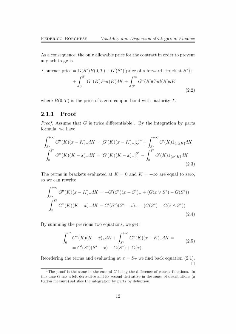
The weights (which have unit sum) are:
wit =NOSHi · Sit
Vt=wi0 · SitVt · Si0
The weights change every day and the best performing stocks see theirweight increase. Observe that, after a long period of time, stock pricescan go very far from the initial price, so the strategy will become moreand more similar to holding the best performing stocks (and less de-pendent on correlation).Most of the times, when people say “a basket 60% SX5E, 30% UKXand 10% SMI ” they don’t mean that the weights are fixed at 60%,30%and 10% but rather that the NOSH is fixed. The value of the basketthey refer to is
Vt = 60%SX5Et
SX5E0
+ 30%UKXt
UKX0
+ 10%SMItSMI0
(2.22)
• Arithmetic baskets: they are a special case of the above. An arith-metic basket starting at time 0 is defined as
Bt =1
n
n∑i=1
SitSi0
(2.23)
Therefore,∆Bt
Bt
=n∑i=1
SitnSi0Bt
∆SitSit
, so the weights are wit =Sit
nSi0Bt
• The Euro Stoxx 50 (SX5E Index). This is a basket of the 50 largestEuropean companies. It rebalances every 3 months, and between tworebalancing dates it holds a fixed number of shares. Let k be a rebal-ancing date and wik the weight of stock i for i = 1, ..., 50. Then
∆SX5Ek
SX5Ek
=50∑i=1
wik∆SikSik
(2.24)
The number of shares of stock i is then NOSHi =wikSX5Ek
Sik. Hence,
the effective weights of the Euro Stoxx 50 are
wit =wik · SX5Ek · SitSik · SX5Et
(2.25)
17

Federico Borghese Volatility and Dispersion strategies in Finance
Observe that these weights, differently from the previous cases, re-main meaningful as time passes because of the rebalancing. Over three
months,SX5Ek · SitSik · SX5Et
rarely becomes significantly different than 1, so,
with a good approximation, we could say that the EuroStoxx has con-stant weights wit = wik for every 3-month period.
18

Chapter 3
Volatility products
3.1 Introduction
Volatility is one of the most important quantities in financial markets, givenits key role in determining the price and the hedge of derivatives, in eval-uating an asset’s performance (e.g. Sharpe Ratio), in designing investmentstrategies and Smart Beta Indices.Volatility is a measure of the way a stochastic process moves around its trend.A very smooth stochastic process, for example the value of a strategy whichinvests in money market instruments has almost zero volatility. On the otherhand, the price of a share of a company can be very volatile, especially intimes of uncertainty and during market stress. The more volatile is a stock,the harder it is to predict its price in one month, the more expensive will bea Call or Put option on that stock. On the other hand, the most volatileassets offer the chances of the highest returns.Volatility is a quantity which is not directly measurable. Within the clas-sical Black-Scholes model, volatility is a parameter of the model and thereare many good estimators of it. However there is evidence from data thatvolatility is not constant at all: it is not constant over time and even ata given time it varies depending on the strike and maturity of the option(volatility smile). Actually, volatility does not exist : in theory it should bethe instantaneous rate at which a stochastic process is oscillating, which isimpossible to measure or properly define, and volatility itself is a stochasticprocess.While there are a variety of models which introduce a stochastic diffusionfor the volatility (Dupire’s local volatility, Heston’s model and many othermodern models), it is not in the scope of this document to treat them. Theway we can treat volatility is the following: well defining different types of
19
Federico Borghese Volatility and Dispersion strategies in Finance
volatilities and understanding the meaning and the relationships betweenthem.
3.1.1 Implied Volatility
Implied volatility is not a completely trivial quantity to understand. It canbe seen as a forward-looking measure of how much the price will oscillate inthe future. It is a quantity which is implied by the market, i.e. it is derivedmy the market price of products which depend on volatility. These productsare Call and Put options, which in most cases are the most liquid derivativeproduct available in the market. Therefore, implied volatility refers to:
• An underlying
• A particular strike
• A particular maturity
Definition 3.1. The implied volatility of the underlying S, at strike K andmaturity T , is the volatility that, input to Black-Scholes pricing model, yieldsa theoretical price of a vanilla option with strike K and maturity T equal tothe current market price of the option.
The way implied volatility can be seen is simply as a more convenient way toexpress a price. Currency prices are not the most expressive way to describethe price of an option: it is hard to compare a price of 7 USD for a 1Yat-the-money Call Option on the S&P 500 and a price of 150 EUR for a 2YQuanto Straddle on the Nikkei 225. But it becomes meaningful to comparetheir implied volatilities which are expressed in the same units.
3.1.2 Realized Volatility
Realized volatility is a backwards-looking quantity, which measures howmuch the price has oscillated in a well specified time period.
Definition 3.2. The daily Realized Variance of an Underlying S in theperiod [t, T ] (expressed in number of days) is the following quantity:
σ2t,T :=
252
T − t
T∑u=t+1
ln
(SuSu−1
)2
(3.1)
20

Federico Borghese Volatility and Dispersion strategies in Finance
The daily Realized Volatility is the square root of the Realized Variance,i.e.
σt,T :=
√√√√ 252
T − t
T∑u=t+1
ln
(SuSu−1
)2
The length of the time period is expressed as a number of businessdays (T − t) divided by the total number of business days in one year (byconvention, 252).
Proposition 3.3. (Additivity property): The realised variance is additiveon adjacent time periods. In formulas,
(T3 − T1)σ2T1,T3
= (T2 − T1)σ2T1,T2
+ (T3 − T2)σ2T2,T3
(3.2)
Proof. By definition (3.1), the right hand side is equal to
252
T2∑u=T1+1
ln
(SuSu−1
)2
+ 252
T3∑u=T2+1
ln
(SuSu−1
)2
Combining the sums gives exactly the definition of (T3 − T1)σ2T1,T3
.
The are other possibilities for measuring the realised volatility. Forexample, instead of taking daily returns, we could introduce a picking fre-quency of, let’s say, 5, and use 5-day returns in the previous formula. This isparticularly appropriated when measuring the volatility of a basket of assetsbelonging to different geographical areas. We will come back to this topic insection 4.1.4.Also, some people take different formulas for realised volatility, for examplethe standard deviation of the log-returns:
σ2t,T :=
252
T − t− 1
T∑u=t+1
[ln
(SuSu−1
)− 1
T − t
T∑v=t+1
ln
(SvSv−1
)]2
(3.3)
In most cases, the underlying price has a very small drift, so the two formulasgive almost the same result. However, the latter formula excludes the driftand only measures the oscillating side of the price evolution. When comput-ing the realised volatility in a hypothetical scenario where interest rates are10%, the differences between the two formulas arise. A major inconvenienceof this formula is that the additivity property is lost.
21

Federico Borghese Volatility and Dispersion strategies in Finance
Realised volatility in a stochastic volatility model
If we assume a diffusive continuous model for the Underlying’s price withstochastic volatility, that is
dStSt
= µtdt+ σtdBt (3.4)
then it is natural to define the realized variance as
σ2t,T =
1
T − t
∫ T
t
σ2udu
Actually, the definition given in (3.1) is a good approximation of the lattertheoretical realized variance. In fact, if we assume the model (3.4), by Ito’sformula we have
d ln(St) = (µt −1
2σ2t )dt+ σtdWt (3.5)
Under suitable integrability assumptions, ln(St) is a continuous semimartin-gale. Therefore, by Theorems 1.8 and 1.18 in [1], we have a convergence inprobability of
N∑i=1
(ln(Si TN
)− ln(S(i−1) TN
))2 P−→ 〈ln(St), ln(St)〉 =
∫ T
0
σ2t dt (3.6)
for N → ∞. However, this convergence holds for the time frame used tocompute returns going to zero.
3.2 Variance Swaps
Definition 3.4. A Variance Swap is a forward contract on the annualizedvariance of the Underlying.
As any forward contract, the Variance Swap is an agreement betweentwo counterparties to buy (or sell) at maturity an unknown quantity, inour case the future realized variance, at a certain strike price. Let K2
var bethe strike price of the Variance Swap and σ2
0,T the realized variance of theUnderlying over the period [0, T ]. Then the payoff at maturity of a VarianceSwap expiring at time T is
N(σ20,T −K2
var)
22

Federico Borghese Volatility and Dispersion strategies in Finance
where N is the notional of the contract.In most cases, the Variance Swap notional is expressed in the form of a VegaNotional. The payoff is
(Vega Notional)×σ2
0,T −K2var
2Kvar
× 100
We will see in subsection 3.2.2 the reasons of this choice.
3.2.1 Replication and fair strike of a Variance Swap
Assume that Call and Put options on the underlying are available in themarket. For the moment, let us assume the unrealistic hypothesis that Callsare available for every strike K ≥ S∗ and Puts are available for every strikeK ≤ S∗ (where S∗ is likely to be the ATM or ATMf).
Theorem 3.5. The realized variance σ20,T can be replicated with the following
instruments: a zero-coupon bond, cash, a forward, a delta strategy, vanillaPut and vanilla Call options on the underlying. The replication is given by:
σ20,T =
2
T
[∫ T
0
dStSt− ln
S∗
S0
− ST − S∗
S∗+
+
∫ S∗
0
1
K2(K − ST )+dK +
∫ ∞S∗
1
K2(ST −K)+dK
] (3.7)
The previous theorem allows us to derive the fair strike of a VarianceSwap. Assume the existence of a constant, risk-free rate r to remain ina simple framework (even though it would be more appropriate to use astochastic rate), and let Q be the risk-neutral measure. The fair strike Kvar
is the strike which makes the value of the contract equal to zero. The valueof the contract is e−rtEQ
[N(σ2
0,T −K2var)], therefore the fair strike satisfies
K2var = EQ
[σ2
0,T
](3.8)
Under the risk-neutral measure Q we have that
dStSt
= rdt+ σtdBt
23

Federico Borghese Volatility and Dispersion strategies in Finance
where Bt is a Q-Brownian Motion. Therefore,
EQ
[∫ T
0
dStSt
]= rT ; (3.9)
EQ
[ST − S∗
S∗
]=S0e
rT − S∗
S∗; (3.10)
EQ
[∫ S∗
0
1
K2(K − ST )+dK
]= erT
∫ S∗
0
1
K2Put(K)dK (3.11)
EQ
[∫ ∞S∗
1
K2(ST −K)+dK
]= erT
∫ ∞S∗
1
K2Call(K)dK (3.12)
Combining the previous equations, we find that
K2var =
2
T
[lnS0e
rT
S∗−(S0e
rT
S∗− 1
)+
+ erT∫ S∗
0
1
K2Put(K)dK + erT
∫ ∞S∗
1
K2Call(K)dK
] (3.13)
3.2.2 Sensitivities
What is in the interest of the trader are the Greeks of the portfolio of VanillaOptions used for replicating the Variance Swap. The portfolio in considera-tion is
Πt =2
T
[∫ S∗
0
1
K2Putt(K)dK +
∫ ∞S∗
1
K2Callt(K)dK
](3.14)
What the trader will do is to hedge with a discrete version of equation 3.7:holding as many options as possible, suitably weighted1, and replicating the
term2
T
∫ T
0
dStSt
with the daily rebalanced strategy2
T
T∑t=1
1
St−1
(St − St−1).
Observation 3.6. The term2
T
∫ T
0
dStSt
present in the replication of the Vari-
ance Swap has different sensitivities than the effective strategy implemented
by the trader2
T
T∑t=1
1
St−1
(St − St−1). For example, the former has a Gamma
of∂
∂St
(2
TSt
)= − 2
TS2t
and the latter has a Gamma of zero.
1See section 3.4 for more precise details
24

Federico Borghese Volatility and Dispersion strategies in Finance
Assume for simplicity that interest rates are zero. We can considerequation (3.13) for the period [t, T ], obtaining
K2t,T =
2
T − t
[lnStS∗−(StS∗− 1
)+
+
∫ S∗
0
1
K2Putt(K)dK +
∫ ∞S∗
1
K2Callt(K)dK
] (3.15)
Hence we find
Πt =T − tT
K2t,T −
2
TlnStS∗
+2
T
(StS∗− 1
)(3.16)
From the above equation we can find all the Greeks.
Vega
The Vega of a Variance Swap coincides with the Vega of the option portfolio,because in the replication (3.7) it is the only vega-sensitive term.
νt =∂Π
∂Kt,T
= 2T − tT
Kt,T (3.17)
Very often the notional of Variance Swaps is expressed as a Vega Notionaldivided by 2 times the Variance Swap initial strike. To clarify,
Notional = 100Vega Notional
2K0,T
This can be explained looking at the above sensitivity: at inception, the
Vega of 100NV ega
2KVariance Swaps is exactly 100Nvega. Therefore, if volatility
increases by one point, the value of the contract increases by 100Nvega×1% =Nvega. This means that the Vega Notional is the amount of money which isgained or lost when volatility moves by 1%. However this is only true atinception and not anymore during the life of the contract.Another way to derive the Vega of a Variance Swap is by using the additivityproperty (3.2). Since σ2
0,T = tTσ2
0,t + T−tTσ2t,T , the Mark-to-Market at time t
of the variance is
MTMt =t
Tσ2
0,t +T − tT
K2t,T (3.18)
Therefore the Vega of the Variance Swap is
νt =∂MTMt
∂Kt,T
= 2T − tT
Kt,T (3.19)
25

Federico Borghese Volatility and Dispersion strategies in Finance
Delta
∆t =∂Π
∂St= − 2
TSt+
2
TS∗(3.20)
We can observe that the Delta of the option portfolio is hedged by the deltastrategy
∫dStSt
and the forward present in the Variance Swap replication (3.7).After all, the Delta of the Variance Swap must be zero.
Gamma
Γt =∂2Π
∂S2t
=2
TS2t
(3.21)
Gamma is always positive, but it will be balanced by the always negativeTheta. We observe that the Gamma faced by the trader is not zero, whereasthe Gamma of a Variance Swap is zero (having a Variance Swap aconstantly zero Delta). The discrepancy is caused by the fact that the trader
implements a daily rebalanced strategy2
T
T∑t=1
1
St−1
(St−St−1) which has zero
Gamma. If the trader implemented the continuously rebalanced strategy2
T
∫ T
0
dStSt
he would see an additional Gamma of∂
∂St
(2
TSt
)= − 2
TS2t
which
would bring the total Gamma to zero.
Theta
θt =∂Π
∂t= − 1
TK2t,T (3.22)
We see that Theta is always negative, and we see that the Gamma profit12ΓS2σ2dt is equal to the Theta loss −θdt.
Although less intuitively, the Theta can also be found thanks to the additivityproperty. From equation (3.18), we have
MTMt+dt =t+ dt
Tσ2
0,t+dt +T − t− dt
TK2t+dt,T (3.23)
By another application of the additivity property, we have
(t+ dt)σ20,t+dt = tσ2
0,t + dt · σ2t,t+dt (3.24)
When computing the Theta, we assume that spot and volatility do not move,i.e. σ2
t,t+dt = 0 and K2t+dt,T = K2
t,T . Hence
θt =MTMt+dt −MTMt
dt= − 1
TK2t,T (3.25)
26

Federico Borghese Volatility and Dispersion strategies in Finance
Vanna
The Vanna of the option portfolio coincides with the Vanna of the VarianceSwap.
V annat =∂2Π
∂St∂Kt,T
= 0 (3.26)
This means that the Vega of the Variance Swap is independent of the spot,which translates the fact that a Variance Swap give pure exposure to volati-lity.
3.2.3 Derivation of the replication in a stochastic vo-latility model
Assume for the Underlying price a continuous diffusion model with no jumps,with the volatility being a stochastic process. That is, we assume that theprice evolution is given by
dStSt
= µtdt+ σtdBt
where Bt is a standard Brownian Motion under the Historical Probability.
The realized variance is the sum of a delta strategy and a log con-tract
By Ito’s formula we have
d ln(St) = (µt −1
2σ2t )dt+ σtdWt =
dStSt− 1
2σ2t dt (3.27)
By integrating both sides of the previous equation from t to T we obtain
lnSTS0
=
∫ T
0
dStSt− 1
2
∫ T
0
σ2t dt (3.28)
The realized variance over the period [0, T ] is σ20,T = 1
T
∫ T0σ2t dt, therefore we
obtain that
σ20,T =
2
T
[∫ T
0
dStSt− ln
STS0
](3.29)
The second term in the brackets is an European option on the underlying,since it is a function of the final price of S. We will refer to it as a log con-tract.The first term in the brackets can be thought as the final value of a Delta
27
Federico Borghese Volatility and Dispersion strategies in Finance
strategy in the underlying. This strategy has initial value of rTe−rT , re-balances continuously and is instantaneously long 1
Ste−r(T−t) shares of the
underlying. In fact, let Vt be the value of a self-financed portfolio holding1Ste−r(T−t) shares and V0 = rTe−rT ; being the strategy self-financed, we can
write
d(e−rtVt) =1
Ste−r(T−t)d(e−rtSt) =
1
Ste−r(T−t)(e−rtdSt − re−rtStdt) (3.30)
By integrating both sides we obtain
VT e−rT − V0 = e−rT
∫ T
0
dStSt− rTe−rT (3.31)
and finally, substituting V0, we find
VT =
∫ T
0
dStSt
The log contract can be replicated with a strip of vanilla Calls andPuts
The log contract is an European payoff, therefore we can replicate it withvanilla options according to Carr’s formula (2.1). G(x) = − ln x
S0is twice
differentiable, with G′(x) = − 1x
and G′′(x) = 1x2
. Hence,
− lnSTS0
= − lnS∗
S0
− ST − S∗
S∗
+
∫ S∗
0
1
K2(K − ST )+dK +
∫ ∞S∗
1
K2(ST −K)+dK
(3.32)
Combining this result with equation (3.29) concludes the proof.
3.3 Variations of Variance Swaps
In this section we will show results similar to the already obtained on VarianceSwaps, but applied to variations such as Conditional Variance Swaps andGamma Swaps.
3.3.1 Corridor Variance Swaps Definitions
Corridor variance swaps make it possible to be exposed to the variance condi-tionally to the price of the underlying being in a specified range. For example,
28

Federico Borghese Volatility and Dispersion strategies in Finance
an investor might want to sell realised variance, but to freeze his exposure inthe event of a market crash. He could achieve this by entering an Up Vari-ance Swap, which will provide exposure to the “normal conditions” volatilityand not to the “stress conditions” volatility.
Definition 3.7. The (non-normalized) corridor realised variance of an un-derlying with price St, with barriers Ldown, Lup is the following quantity:
σ2non−norm =
252
T − t
T∑u=t+1
ln
(SuSu−1
)2
1{Ldown≤Su−1≤Lup} (3.33)
The (non-normalized) Up Variance is a corridor variance with Lup =+∞ and the (non-normalized) Down Variance is a corridor variance withLdown = 0.
Definition 3.8. A (non-normalized) Corridor Variance Swap is a forwardcontract on the realised Corridor Variance. Hence the payoff of an Corri-dor Variance Swap with maturity T , strike K2
corr, notional N and barriersLdown, Lup is
N(σ2non−norm −K2
corr
)(3.34)
A Down Variance Swap and an Up Variance Swap are, similarly, forwardcontracts on the Down Variance and the Up Variance.
In order to have a quantity which is comparable to realised variance,it is more meaningful to normalise by taking a conditional average of thesquared log returns:
Definition 3.9. The Corridor Realised Variance of an underlying with priceSt, with barriers Ldown, Lup is the following quantity:
σ2corr =
252T∑
u=t+1
1{Ldown≤Su−1≤Lup}
T∑u=t+1
ln
(SuSu−1
)2
1{Ldown≤Su−1≤Lup} (3.35)
The Up Variance is a corridor variance with Lup = +∞ and the DownVariance is a corridor variance with Ldown = 0.
Set
Ncond =T∑
u=t+1
1{Ldown≤Su−1≤Lup} (3.36)
Ncond is the number of days where the underlying lies in the specified range.It can be seen as a strip of digital options, and we have
Ncondσ2corr = (T − t)σ2
non−norm
29

Federico Borghese Volatility and Dispersion strategies in Finance
Definition 3.10. A Corridor Variance Swap on the period [0, T ], with no-tional N , has the following payoff:
Payoff = N · Ncond
T
(σ2corr −K2
cc
)= N
(σ2non−norm −
Ncond
TK2cc
)(3.37)
It is crucial that in the payoff usually there is the factor Ncond. This waythe Corridor Variance Swap is equal to a non-normalised Corridor VarianceSwap plus a strip of digital options. The key problem in both definitions isto replicate the quantity σ2
non−norm.
3.3.2 Up Variance Replication
The replication of the Up Variance can be obtained through similar mathe-matical proofs as in the case of standard Variance Swaps. However, this caserequires more sophisticated tools in order to deal with the discontinuity atthe barrier.The main ideas in the Variance Swap replication are:
• Apply Ito’s formula to the function G(x) = lnx
• Identify the estimator of the variance (the real underlying of the con-tract) with the theoretical quantity in the model
• Express the realised variance in terms of a delta strategy, plus G(ST )
• Replicate the European Payoff G(ST ) with vanilla options according toCarr’s formula
We can use the same ideas, but we need to find a suitable function G. LetL be the down barrier. Intuitively, G must behave like lnx for x ≥ L andG(x) = 0 for x < L. Most importantly, we ask G to be as regular aspossible, in order to apply Ito and Carr formulas. Searching G of the formG(x) = (a+ bx+ lnx)1{x≥L}, and imposing the constraints that both G andG′ be continuous at L, we find
G(x) =
(− 1
L(x− L) + ln
x
L
)1{x≥L}
G′(x) =
(− 1
L+
1
x
)1{x≥L}
30

Federico Borghese Volatility and Dispersion strategies in Finance
G is a concave function; its second derivative in the distributional sense isminus a positive Radon measure, which is absolutely continuous with respectto Lebesgue measure. The Radon-Nikodym derivative is
G”(x) = − 1
x21{x≥L}
We can apply Ito-Tanaka’s formula combined with the Occupation Timesformula (Equation (2.6)). We obtain:
G(ST )−G(S0) =
∫ T
0
G′(St)dSt +1
2
∫ T
0
G”(St)S2t σ
2t dt
G(ST )−G(S0) =
∫ T
0
(− 1
L+
1
St
)1{St≥L}dSt −
1
2
∫ T
0
σ2t 1{St≥L}dt (3.38)
In the last term we recognise the Up Variance. The central term is a deltastrategy in the underlying. Therefore,
UpV ariance =1
T
∫ T
0
σ2t 1{St≥L}dt =
=2
T
[−G(ST ) +G(S0) +
∫ T
0
(− 1
L+
1
St
)1{St≥L}dSt
] (3.39)
The last step for finding the replication of the Up Variance with vanillainstruments is to decompose the European Payoff G(ST ) as a combinationof Calls and Puts. Since we designed G to be regular enough, we can applyCarr’s formula (2.1), with S∗ = L. Since G(L) = G′(L) = 0, we find
G(ST ) = −∫ +∞
L
1
K2(ST −K)+dK
In conclusion
UpV ar =2
T
[G(S0) +
∫ T
0
(− 1
L+
1
St
)1{St≥L}dSt +
∫ +∞
L
1
K2(ST −K)+dK
](3.40)
Observation 3.11. Should there not be any available Call option with strikebetween L and 100%, it is always possible to build a synthetic Call optionusing a Put, the Forward and cash, thanks to the Call-Put parity.
31

Federico Borghese Volatility and Dispersion strategies in Finance
3.3.3 Weighted Variance Swap replication
Inspired by the ideas in the previous section, we can generalize the Ito-Tanakacombination with Carr formula methodology.Take G : R+ → R satisfying the following hypotheses:
• G is continuous and differentiable
• G is the difference of two convex functions (automatically satisfied ifG is C2);
• the second derivative of G in the distributional sense (which is a Radonmeasure) is absolutely continuous with respect to Lebesgue measure,with Radon-Nikodym derivative denoted as G”.
By equation (2.6) we have that
G(ST )−G(S0) =
∫ T
0
G′−(St)dSt +1
2
∫ T
0
G”(St)S2t σ
2t dt (3.41)
Set w(x) := −G”(x)x2 . Then we find
1
T
∫ T
0
w(St)σ2t dt =
2
T
[−G(ST ) +G(S0) +
∫ T
0
G′(St)dSt
](3.42)
As we previously did, we decompose the European Payoff G(ST ) as a combi-nation of Calls and Puts. Since we designed G to be regular enough, we canapply Carr’s formula (2.1). We find
G(ST ) = G(S∗) +G′(S∗)(ST − S∗)−
−∫ S∗
0
w(K)
K2(K − ST )+dK −
∫ ∞S∗
w(K)
K2(ST −K)+dK
(3.43)
Combining the previous two, we finally get
1
T
∫ T
0
w(St)σ2t dt =
2
T
[G(S0)−G(S∗)−G′(S∗)(ST − S∗) +
∫ T
0
G′(St)dSt+
+
∫ S∗
0
w(K)
K2(K − ST )+dK +
∫ ∞S∗
w(K)
K2(ST −K)+dK
](3.44)
Definition 3.12. The Weighted Realised Variance of an underlying St withweighting w(x) is the following quantity:
σ2w =
252
T
T∑u=1
w (Su−1)
(ln
SuSu−1
)2
(3.45)
32

Federico Borghese Volatility and Dispersion strategies in Finance
Similarly to what we did in the case of the Variance Swap, we can
identify the Weighted Realised Variance with the quantity1
T
∫ T
0
w(St)σ2t dt.
The previous equation gives us the way to replicate any Weighted RealisedVariance:
1. Identify the weight w(x);
2. Solve the differential equation G”(x) = −w(x)
x2(initial conditions do
not matter2); by solving we mean finding a function G such that:
(a) G is continuous and differentiable
(b) G is the difference of two convex functions (automatically satisfiedif G is C2);
(c) the second derivative of G in the distributional sense (which is aRadon measure) is absolutely continuous with respect to Lebesgue
measure, with Radon-Nikodym derivative equal to −w(x)
x2;
3. Use equation (3.44) to find the replication.
3.3.4 Gamma Swaps
Gamma Swaps are an alternative to Variance Swaps for getting exposure tofuture realized variance. The main advantages of a Gamma Swap is thatit provides exposure to realised variance and it is perfectly replicable withVanilla options (as the Variance Swap), but it avoids explosions in marketcrashes and usually has a lower strike. The Gamma Swap market has neverreached a satisfactory liquidity, however Gamma Swaps are still found inmany OTC trades.
Definition 3.13. A Gamma Swap on the underlying S with maturity T isa forward contract on the following quantity3:
ς2 =252
T
T∑t=1
StS0
[log
StSt−1
]2
(3.46)
2By simple calculations, the reader can see that equation (3.44) is invariant for the
transformation G(x)→ G(x) = G(x)+α+βx. Therefore, any G satisfying G”(x) = −w(x)x2
will produce the same result.
3Alternative definitions include ς2 = 252T
T∑t=1
St−1
S0
[log St
St−1
]2. The difference is minimal.
33

Federico Borghese Volatility and Dispersion strategies in Finance
The above quantity is very similar to the realized variance. The differ-ence is that log-returns are weighted by the relative move in the spot. Thisway, when the spot goes down and volatility increases, the Gamma Swapreduces its volatility exposure and avoids blowing up like a Variance Swap.The replication of a Gamma Swap is easily obtained from equation (3.44),with a weight w(x) = x
S0. A function G which satisfies the differential equa-
tion
G”(x) = −w(x)
x2= − 1
S0x(3.47)
is easily found, for example G(x) = − xS0
(log x
S0− 1)
, which satisfies all the
requested hypotheses. In the case of the Gamma Swap, we find
1
T
∫ T
0
StS0
σ2t dt =
2
T
[G(S0)−G(S∗)−G′(S∗)(ST − S∗) +
∫ T
0
G′(St)dSt+
+1
S0
∫ S∗
0
1
K(K − ST )+dK +
1
S0
∫ ∞S∗
1
K(ST −K)+dK
](3.48)
We see that the weights of the Vanillas are 1K
compared to the 1K2 of the
Variance Swap. This means that the Gamma Swap replication makes use ofless OTM Puts and more OTM Calls than the Variance Swap, and so it hasless sensitivity to the skew and lower strike.In the particular case S∗ = S0, we have G′(S0) = 0 and from equation (3.48):
Gamma Swap Quantity = ς2[0,T ] =
252
T
T∑t=1
StS0
[log
StSt−1
]2
≈
≈ 2
S0T
[−∫ T
0
logStS0
dSt +
∫ S0
0
1
K(K − ST )+dK +
∫ +∞
S0
1
K(ST −K)+dK
](3.49)
Weighted additivity property for Gamma Swaps
Similarly to what we proved in Proposition 3.3, we prove a weighted addi-tivity property for the Gamma Swap quantity
ς2[t,T ] =
252
T − t
T∑u=t+1
SuSt
[log
SuSu−1
]2
34
Federico Borghese Volatility and Dispersion strategies in Finance
Proposition 3.14. (Weighted additivity property for a Gamma Swap):The realised Gamma Swap quantity ς2
[t,T ] satisfies the following relation:
ς2[0,T ] =
t
Tς2[0,t] +
T − tT
StS0
ς2[t,T ] (3.50)
Proof. By definition, the right hand side is equal to
t
T· 252
t
t∑u=1
SuS0
ln
(SuSu−1
)2
+StS0
T − tT· 252
T − t
T∑u=t+1
SuSt
ln
(SuSu−1
)2
(3.51)
Combining the sums gives exactly the definition of ς2[0,T ].
Sensitivities
As in the case of a Variance Swap (section 3.2.2), we investigate the Greeksof the Gamma Swap and of option portfolio which replicates the GammaSwap. The portfolio in consideration is
Πt =2
S0T
[∫ S∗
0
1
KPutt(K)dK +
∫ ∞S∗
1
KCallt(K)dK
](3.52)
Assume for simplicity that interest rates are zero. We can consider equation
(3.48) for the period [t, T ], with G(x) = − xSt
(log x
St− 1)
and S∗ = S0,
obtaining
1
T − t
∫ T
t
SuStσ2udu =
2
T − t
[1− S0
St+STSt
logS0
St+
∫ T
0
G′(St)dSt+
+1
St
∫ S0
0
1
K(K − ST )+dK +
1
St
∫ ∞S0
1
K(ST −K)+dK
](3.53)
Let K2[t,T ] be the strike of the Gamma Swap on the period [t, T ]: taking the
risk-neutral expectation of the above equation, we have
K2[t,T ] =
2
T − t
[1− S0
St+ log
S0
St
]+
T
T − t· S0
StΠt (3.54)
Πt =StS0
· T − tT
K2t,T −
2
S0T
(St − S0 + St log
S0
St
)(3.55)
From the above equation we can find all the Greeks. In particular, we findthe Delta and the Gamma.
35

Federico Borghese Volatility and Dispersion strategies in Finance
Delta
∆t =∂Π
∂St=
1
S0
· T − tT
K2t,T +
2
TS0
logStS0
(3.56)
We observe that the Delta of the option portfolio is not totally hedged bythe delta strategy
∫ T0
log StS0dSt present in the replication. The Delta of the
Gamma Swap is not zero, but1
S0
· T − tT
K2t,T . Alternatively, this can easily
be seen from the additivity property of the Gamma Swap.
Gamma
Γt =∂2Π
∂S2t
=2
TS0St(3.57)
Opposed to the Variance Swap, where the Gamma was proportional to 1S2t,
in the case of the Gamma Swap the Gamma is proportional to 1St
. The shareGamma is defined by the rate of change in the Delta for a small percentreturn (dSt
St) of the underlying, i.e.
Share Gamma = StΓ =∂∆∂StSt
We see that in the case of the Gamma Swap, the share Gamma is constant.
Observation 3.15. Similarly to the case of the Variance Swap, there is adiscrepancy between the Gamma faced by the trader and the Gamma of aGamma Swap. The Gamma Swap’s Delta is equal to
Gamma Swap Delta =1
S0
· T − tT
K2t,T
Hence, the Gamma of a Gamma Swap is equal to zero. The trader
will replicate the strategy − 2
T
∫ T
0
logStS0
dSt with a daily rebalanced strategy
− 2
T
T∑t=1
logSt−1
S0
(St−St−1) which has zero Gamma. If he instead rebalanced
continuously, his additional Gamma would be − ∂
∂St
(log
StS0
)= − 2
TS0St.
Therefore his total Gamma would be zero.
36

Federico Borghese Volatility and Dispersion strategies in Finance
3.3.5 Corridor Variance Swap Replication
In this case the weight is w(x) = 1{L≤x≤U}. The differential equation G”(x) =
−w(x)x2
is solved by
G(x) =
0 if 0 ≤ x ≤ L
− 1L
(x− L) + ln xL
if L ≤ x ≤ U(1U− 1
L
)x+ ln U
Lif U ≤ x
(3.58)
Therefore,
CorrV ar =1
T
∫ T
0
1{L≤St≤U}σ2t dt =
=2
T
[G(S0)−G(S∗)−G′(S∗)(ST − S∗) +
∫ T
0
G′(St)dSt+
+
∫ S∗
L
1
K2(K − ST )+dK +
∫ U
S∗
1
K2(ST −K)+dK
](3.59)
3.3.6 Re-finding the Variance Swap
In this case the weight is w(x) = 1. The differential equation G”(x) = − 1x2
issolved by G(x) = ln x and equation (3.44) yields the same result as previouslyfound in equation (3.7).
3.3.7 Volatility Swaps
Definition 3.16. A Volatility Swap is a forward contract on realized vola-tility, i.e. on the square root of realized variance.
Let Kvol be the strike price of the Volatility Swap and σ20,T the realized
variance of the Underlying over the period [0, T ]. Then the payoff at maturityof a Variance Swap expiring at time T is
N(√σ2
0,T −Kvol)
where N is the notional of the contract.The interest of a volatility swap lies in the fact that it reduces the losses of theseller due to a potential spike in realised variance. In the 2008 financial crisis,investment banks incurred in huge losses on their short positions on varianceswaps, and later on variance swaps have always been capped. Volatility
37

Federico Borghese Volatility and Dispersion strategies in Finance
swaps are a safer alternative to sell: if volatility increases from 20% to 60%,a volatility swap pays 40% whereas a variance swap with same vega notionalpays 1
2×20%((60%)2 − (20%)2) = 80%.
Strike of a Volatility Swap
Volatility swaps are not replicable with vanilla options like variance swaps. Avolatility swap can be seen as a derivative on variance as underlying, thereforeit is sensitive to the so-called vol of vol (or vol of var). A model of diffusionof variance is needed for the fair strike of the volatility swap. The Hestonmodel is a classical example of a stochastic volatility model, but even withthe model assumptions there is no closed-form formula for the strike of avolatility swap.What can be said independently of the model is that the fair strike of avolatility swap is always lower than the fair strike of a variance swap. Thereare two easy ways to see it:
• (Financial Way) A long position on volatility is short vol of vol, there-fore the fair strike has to be reduced to compensate the investor for thesale of vol of vol.
• (Mathematical Way) Let σ be the future realised volatility. We have
0 ≤ V ar[σ] = E[σ2]− E[σ]2 = K2var −K2
vol (3.60)
That proves the inequality. Moreover, we see that the difference be-tween the two squared strikes is the variance of the future realisedvolatility. The strikes coincide only if σ is deterministic (i.e. zero volof vol, but also no point in trading variance swaps). The more vol ofvol, the higher V ar[σ], the higher the spread.
What we just proved can be put in a proposition:
Proposition 3.17. The convexity bias, i.e. the spread between the strikesof a Variance Swap and a Volatility Swap on the same underlying and samematurity, is
Convexity Bias = K2var −K2
vol = V ar[σ0,T ] (3.61)
where the Variance of σ is taken under the risk-neutral measure.
3.4 Backtest
We backtested the replication of realized variance explained in Theorem 3.5.The strip of options is approximated by a discrete number of options weighted
38

Federico Borghese Volatility and Dispersion strategies in Finance
by 1K2 . This is the most crucial approximation in the replication, and the
results will vary dramatically with the choice of the discretization.
Details of the Backtest
• The underlying is the EuroStoxx 50 Index and the S&P 500 Index (2backtests).
• The realised variance is the 6-month realised variance, computed withdaily close-to-close log returns.
• The term∫ T
0dStSt
is approximated with a daily rebalanced strategy, thatis ∫ T
0
dStSt≈
T∑t=1
St − St−1
St−1
(3.62)
• S∗ is the ATM strike.
• The replication with 2n options and step h consists in holding n Putsand n Calls. The strikes of the Puts are
Kpn = 1− (n− 1)h, ... , Kp
2 = 1− h, Kp1 = 1
with respective weightsh
(Kpn)2 , ...,
h
(Kp2 )2 ,
h
2 (Kp1 )2 . The strikes of the
Calls are
Kcn = 1 + (n− 1)h , ... , Kc
2 = 1 + h, Kc1 = 1
with respective weightsh
(Kcn)2 , ...,
h
(Kc2)2 ,
h
2 (Kc1)2 . Note that the ATM
Call and Put have an additional 12
factor in the weight: this can beexplained mathematically by the trapezoid numerical integration for-mula, or financially by the fact that we have 2 ATM options which buyATM volatility and we don’t want to overweight this ATM volatility.Observe that in any case we are dropping the extremal intervals of thestrikes: the strike range of the options in the market is limited and willnever cover the (0,+∞) theoretical integration interval.
39
Federico Borghese Volatility and Dispersion strategies in Finance
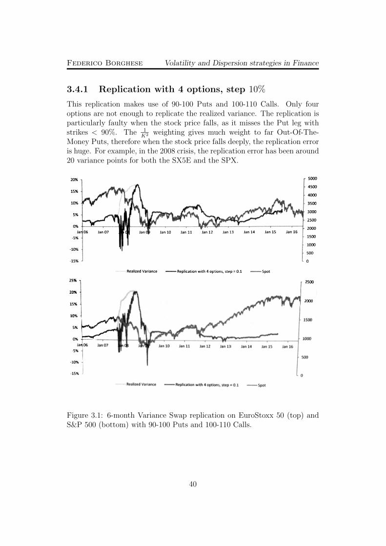
3.4.1 Replication with 4 options, step 10%
This replication makes use of 90-100 Puts and 100-110 Calls. Only fouroptions are not enough to replicate the realized variance. The replication isparticularly faulty when the stock price falls, as it misses the Put leg withstrikes < 90%. The 1
K2 weighting gives much weight to far Out-Of-The-Money Puts, therefore when the stock price falls deeply, the replication erroris huge. For example, in the 2008 crisis, the replication error has been around20 variance points for both the SX5E and the SPX.
Figure 3.1: 6-month Variance Swap replication on EuroStoxx 50 (top) andS&P 500 (bottom) with 90-100 Puts and 100-110 Calls.
40
Federico Borghese Volatility and Dispersion strategies in Finance
3.4.2 Replication with 8 options, step 5%
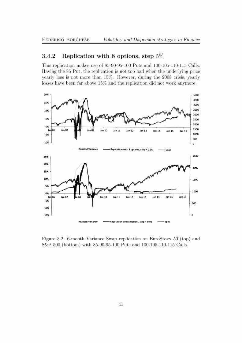
This replication makes use of 85-90-95-100 Puts and 100-105-110-115 Calls.Having the 85 Put, the replication is not too bad when the underlying priceyearly loss is not more than 15%. However, during the 2008 crisis, yearlylosses have been far above 15% and the replication did not work anymore.
Figure 3.2: 6-month Variance Swap replication on EuroStoxx 50 (top) andS&P 500 (bottom) with 85-90-95-100 Puts and 100-105-110-115 Calls.
41

Federico Borghese Volatility and Dispersion strategies in Finance
3.4.3 Replication with 6 options, step 25%
This replication makes use of 50-75-100 Puts and 100-125-150 Calls. Havingthe 50 Put, the replication is not impacted during the crisis. However, mostof the time the underlying yearly return is in the 80-120 area, where thediscretization is too granular. In fact, the replication error is always quitebig.
Figure 3.3: 6-month Variance Swap replication on EuroStoxx 50 (top) andS&P 500 (bottom) with 50-75-100 Puts and 100-125-150 Calls.
42

Federico Borghese Volatility and Dispersion strategies in Finance
3.4.4 Replication with 8 options, step 10%
This replication makes use of 70-80-90-100 Puts and 100-110-120-130 Calls.Having the 70 Put, the replication is rarely a disaster: only when the yearlyloss is above 30%. Also, the discretization is not too granular near the ATMand the replication error is quite small.
Figure 3.4: 6-month Variance Swap replication on EuroStoxx 50 (top) andS&P 500 (bottom) with 70-80-90-100 Puts and 100-110-120-130 Calls.
43
Federico Borghese Volatility and Dispersion strategies in Finance
3.4.5 Replication with 18 options, step 5%
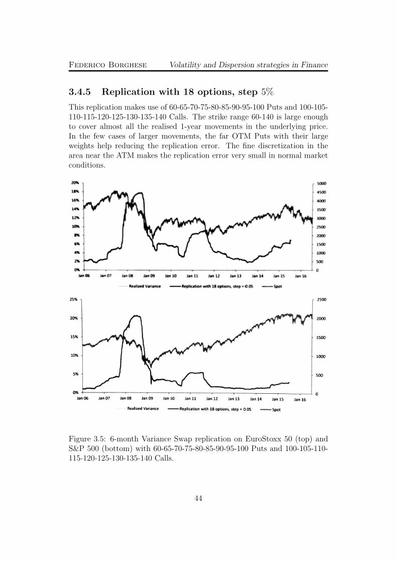
This replication makes use of 60-65-70-75-80-85-90-95-100 Puts and 100-105-110-115-120-125-130-135-140 Calls. The strike range 60-140 is large enoughto cover almost all the realised 1-year movements in the underlying price.In the few cases of larger movements, the far OTM Puts with their largeweights help reducing the replication error. The fine discretization in thearea near the ATM makes the replication error very small in normal marketconditions.
Figure 3.5: 6-month Variance Swap replication on EuroStoxx 50 (top) andS&P 500 (bottom) with 60-65-70-75-80-85-90-95-100 Puts and 100-105-110-115-120-125-130-135-140 Calls.
44
Chapter 4
Correlation
The correlation between the returns of financial assets plays a key role inmodern finance. In financial markets, all securities are dependent from eachother. Interdependent securities don’t necessarily lie within the same assetclass, and the degree of dependence, measured by the correlation coefficient,changes continuously.For example, the price of crude oil and the stock price of an energy companyare usually positively correlated, whereas Equities and Bonds are usuallynegatively correlated. In fact, when Equity markets crash, investors selltheir Equity exposure and buy safer bonds, causing bond prices to rise. Inperiods of bear Equity markets, the correlation between the EuroStoxx 50and the Bund is very negative, but it may happen to be positive in othermarket circumstances.Understanding correlations between financial assets is important to designdiversified strategies, to price derivatives on Equity Indices and also to tradecorrelation itself. Usually, Exotics Trading desks sell correlation to clientsand find themselves very short correlation. Historically, correlation realizes5-10 points below implied correlation, which may drive investors to sell theimplied and buy the realized. For these and many other reasons, a marketof correlation products is born.
4.1 Different types of correlations
4.1.1 Pearson Correlation
In Mathematics there are many ways to express the interdependence of ran-dom variables. The most basic and well-known measure is Pearson’s LinearCorrelation, which expresses the linear dependence between two random
45

Federico Borghese Volatility and Dispersion strategies in Finance
variables. It is defined as:
Definition 4.1. Let X, Y be two random variables. Pearson’s linear corre-lation between X and Y is defined as
ρ =Cov(X, Y )√V ar[X]V ar[Y ]
(4.1)
Given statistical data (x1, y1), ..., (xn, yn), the correlation of the data is thenatural estimator of the above quantity. Set x = 1
n
∑xi and σ2(x) =
1n
∑(xi − x)2 (and similarly for y). Then
ρ =
1n
n∑i=1
(xi − x)(yi − y)
σ(x)σ(y)(4.2)
It is important to understand the faults of this measure:
• A correlation of 0 does not mean that the 2 variables are independent;
• This measure only captures the linear dependence between the vari-ables;
• The standard estimator of the correlation is very noisy, and very sen-sitive to data anomalies;
• It is not suited to measuring the interdependence between 3 or morevariables.
A very educative example is the following. Let X be a N(0, 1) standardGaussian variable, and Y = X2. Clearly, Y is completely determined by X.However,
Cov(X, Y ) = E[XY ]− E[X]E[Y ] = E[X3] = 0 (4.3)
So ρ = 0. Only looking at the value of ρ, we would conclude that there isalmost independence between X and Y , whereas there is complete depen-dence!There are more sophisticated measures of dependence in Mathematics. Cop-ulas are the most complete way to describe the interdependence between nrandom variables; Spearman and Kendall correlations are more robust mea-sures than the linear one. However, despite its faults, the market standardis to use Pearson’s correlation, whose advantages are its simplicity and itseffectiveness in most of the practical cases.
46

Federico Borghese Volatility and Dispersion strategies in Finance
4.1.2 Kendall and Spearman Correlation
Both Spearman correlation ρs and Kendall’s rank correlation coefficient, orτ coefficient, are measures of the rank correlation between two random vari-ables. The two quantities are sensitive only to the ranks of the data, not tothe values, and they are less sensitive to data anomalies. While Pearson’scorrelation captures linear relationships, Spearman and Kendall correlationsassess monotonic relationships (whether linear or not). If there are no re-peated data values, a perfect Spearman or Kendall correlation of +1 or -1occurs when each of the variables is a perfect monotone function of the other.
Spearman Correlation
The Spearman correlation coefficient is defined as the Pearson correlationcoefficient between the ranked variables. To be precise, take statistical data(x1, y1), ..., (xn, yn) and assume that no data value is repeated. We rank thexi and the yi obtaining xi1 > xi2 > ... > xin and yi1 > yi2 > ... > yin . Therank is defined as rk(xij) = j and similarly for y. In other words, the rankof a xi is 1 if it is the largest x observation, 2 if it is the second largest etc.
Definition 4.2. The Spearman Correlation of the data (x1, y1), ..., (xn, yn)is defined as
ρs =
1n
n∑i=1
(rk(xi)− rk(x))(rk(yi)− rk(y))
σ(rk(x))σ(rk(y))(4.4)
Kendall Correlation
Definition 4.3. Let (X, Y ) be a random vector. Take (X ′, Y ′) an i.i.d. copyof (X, Y ). Kendall’s τ correlation between X and Y is defined as
τ = E [sgn((X −X ′)(Y − Y ′))] (4.5)
where sgn denotes the sign function sgn(x) = 1{x>0} − 1{x<0}.
In practice, given statistical data (x1, y1), ..., (xn, yn), the τ coefficientis the natural estimator of the quantity in (4.5), i.e.
τ =1(n2
) n∑i=1
n∑j=1
sgn(xi − xj)(yi − yj) =
=2
n(n− 1)[(number of concordant pairs)− (number of discordant pairs)]
(4.6)
47
Federico Borghese Volatility and Dispersion strategies in Finance
Relationship with Pearson correlation for Gaussian vectors
In this subsection we will find a relationship between Kendall’s τ coefficientand Pearson’s ρ correlation in the case of a bidimensional Gaussian randomvector. Note that this is a special case; it is not possible in general to derivea relationship between the two correlation measures.The result is valid for a bidimensional Gaussian vector. For completeness,we remind the definition:
Definition 4.4. (X, Y ) is said to be a bidimensional Gaussian vector, orto have a bivariate normal distribution, if for every (a, b) ∈ R2, aX + bY isnormally distributed.
Remind that two normally distributed random variables need not be abidimensional Gaussian vector. For example, X ∼ N(0, 1) and
Y =
{X if |X| < 1
−X if |X| ≥ 1(4.7)
are both normally distributed but not a Gaussian vector (because P (X+Y =0) 6= 0 ).
Theorem 4.5. Let (X, Y ) be a Gaussian vector with ρ being Pearson’s cor-relation and τ Kendall’s correlation between X and Y . Then
ρ = sin(τπ
2
)(4.8)
Proof. Taken (X ′, Y ′) an independent copy of (X, Y ) as in the definition ofKendall’s τ , set Z1 = X − X ′, Z2 = Y − Y ′. Since (X, Y ) is a Gaussianvector, then also (Z1, Z2) is a Gaussian vector, with E[Z1] = E[Z2] = 0;V ar[Z1] = 2V ar[X], V ar[Z2] = 2V ar[Y ]. We have
E[Z1Z2] = E[(X −X ′)(Y − Y ′)] =
= E[XY ]− E[X]E[Y ′]− E[X ′]E[Y ] + E[X ′Y ′] =
= 2(E[XY ]− E[X]E[Y ])
(4.9)
So, the correlation between Z1 and Z2 is the same ρ as the correlation betweenX and Y . Being both ρ and τ insensitive to positive affine transformations,we can suppose WLOG that (Z1, Z2) have zero mean and unit variance. Since(Z1, Z2) is a Gaussian vector, we can write
Z2 = ρZ1 +√
1− ρ2Z3 (4.10)
48

Federico Borghese Volatility and Dispersion strategies in Finance
where Z3 ∼ N(0, 1). For this step it is crucial that (Z1, Z2) is a Gaussianvector, otherwise Z3 would not be Gaussian.Now (Z1, Z3) is a standard bivariate Gaussian vector, with Z1, Z3 uncorre-lated therefore independent. Changing the coordinates to polar coordinates,we set {
Z1 = R cos θ
Z3 = R sin θ(4.11)
where R2 has a χ2(2) (or equivalently, exponential) distribution, θ has auniform distribution on [−π
2, 3π
2] and R, θ are independent.
We now compute Kendall’s τ . Let τ ′ ∈ [−1, 1] such that ρ = sin(τ ′π2
). Our
goal is to show that τ = τ ′.
τ = E [sgn(Z1Z2)] = P (Z1Z2 > 0)− P (Z1Z2 < 0) = 2P (Z1Z2 > 0)− 1;(4.12)
P (Z1Z2 > 0) = P[Z1(ρZ1 +
√1− ρ2Z3) > 0
]=
= P[R2 cos θ(ρ cos θ +
√1− ρ2 sin θ) > 0
]=
= P
[cos θ
(sin
(τ ′π
2
)cos θ + cos
(τ ′π
2
)sin θ
)> 0
]=
= P
[cos θ · sin
(θ +
τ ′π
2
)> 0
](4.13)
Now it is a simple trigonometric function sign exercise, which is solved by θbeing either in [− τ ′π
2, π
2] or in [π − τ ′π
2, 3π
2] and giving a probability of
P (Z1Z2 > 0) =1
2π
[(π
2+τ ′π
2
)+
(3π
2− π +
τ ′π
2
)]=
1
2(1 + τ ′) (4.14)
Hence,
τ = 21
2(1 + τ ′)− 1 = τ ′ (4.15)
Example: spot/div correlation
The chart in figure 4.1 analyses the correlation between the EuroStoxx 50Net Total Return Index and its December 2015 dividend futures. For longterm maturities, it is reasonable to think that dividends will be proportionalto the spot level. So we expect a very high correlation between the two assetswhen the maturity is more than 2 years away (which is reflected in the chart
49
Federico Borghese Volatility and Dispersion strategies in Finance
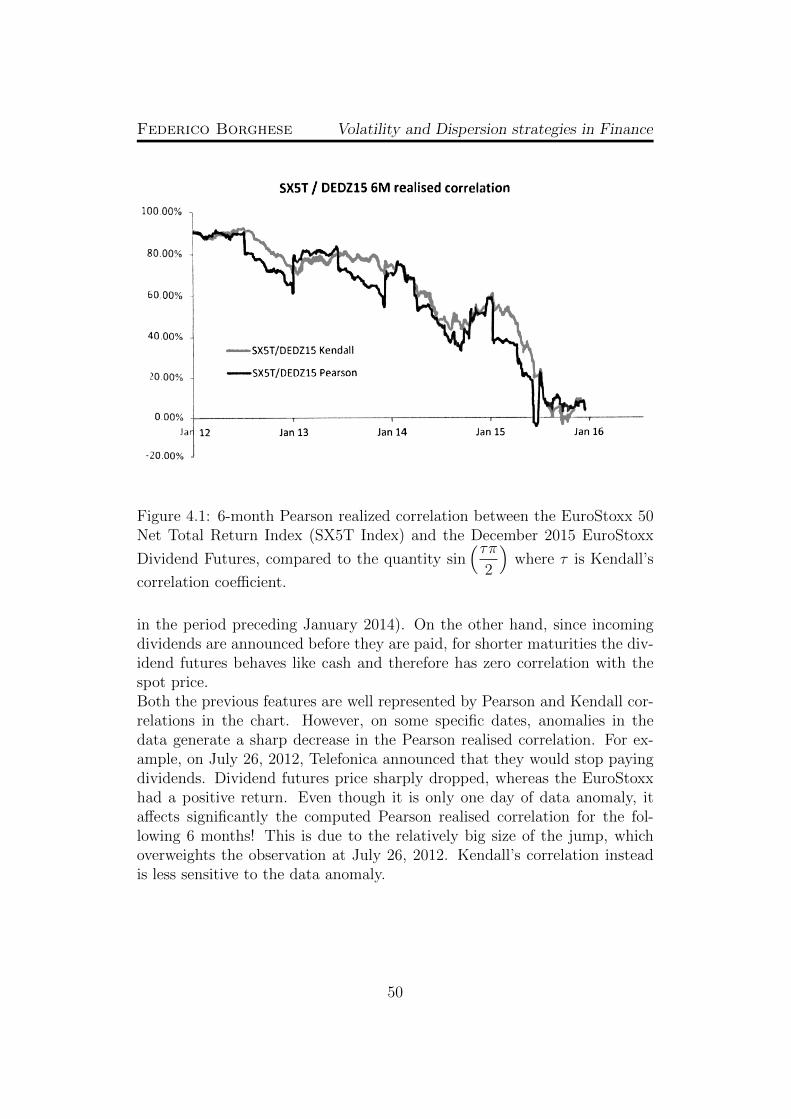
Figure 4.1: 6-month Pearson realized correlation between the EuroStoxx 50Net Total Return Index (SX5T Index) and the December 2015 EuroStoxx
Dividend Futures, compared to the quantity sin(τπ
2
)where τ is Kendall’s
correlation coefficient.
in the period preceding January 2014). On the other hand, since incomingdividends are announced before they are paid, for shorter maturities the div-idend futures behaves like cash and therefore has zero correlation with thespot price.Both the previous features are well represented by Pearson and Kendall cor-relations in the chart. However, on some specific dates, anomalies in thedata generate a sharp decrease in the Pearson realised correlation. For ex-ample, on July 26, 2012, Telefonica announced that they would stop payingdividends. Dividend futures price sharply dropped, whereas the EuroStoxxhad a positive return. Even though it is only one day of data anomaly, itaffects significantly the computed Pearson realised correlation for the fol-lowing 6 months! This is due to the relatively big size of the jump, whichoverweights the observation at July 26, 2012. Kendall’s correlation insteadis less sensitive to the data anomaly.
50

Federico Borghese Volatility and Dispersion strategies in Finance
4.1.3 Correlation in the Black-Scholes model
Given two assets, with price processes S1t , S
2t , we can model their evolution
with a Black-Scholes model:{dS1t
S1t
= µ1dt+ σ1dW1t
dS2t
S2t
= µ2dt+ σ2dW2t
(4.16)
where W 1t , W 2
t are two Brownian motions, not necessarily independent.When saying that S1 and S2 have a correlation of ρ, we mean that thejoint quadratic variation1
d[W 1t ,W
2t ] = ρdt (4.17)
At first sight, this may seem unrelated to Pearson correlation. However, ifwe compute the Pearson correlation of the returns of the assets, assumingthat the parameters µi, σi are constant, we find
Cov
(∆S1
t
S1t
,∆S2
t
S2t
)= Cov(σ1∆W 1
t , σ2∆W 2t ) = E
[σ1σ2∆W 1
t ∆W 2t
]=
= σ1σ2E[∆(W 1
t W2t )−W 1
t ∆W 2t −W 2
t ∆W 1t
](4.18)
By Ito’s formula, we have that
d(W 1t W
2t ) = W 1
t dW2t +W 2
t dW1t + d[W 1
t ,W2t ]
⇒ ∆(W 1t W
2t ) ≈ W 1
t ∆W 2t +W 2
t ∆W 1t + ρ∆t
Combining the previous equations, we find
Cov
(∆S1
t
S1t
,∆S2
t
S2t
)= σ1σ2ρ∆t
Since V ar[∆S1
t
S1t
] = σ21∆t, we conclude that the Pearson correlation of the
returns of the assets is exactly the parameter ρ.Thanks to theorem 4.5, and to the joint Gaussianity of the returns in Black-Scholes model, we can also affirm that
ρ = sin(τπ
2
)(4.19)
where τ is Kendall’s correlation coefficient between the assets’ returns.
Observation 4.6. The previous analysis leads to the same result if we uselog returns instead of linear returns.
1See Chapter Four of [1] for the definition of quadratic variation of semimartingales.
51
Federico Borghese Volatility and Dispersion strategies in Finance
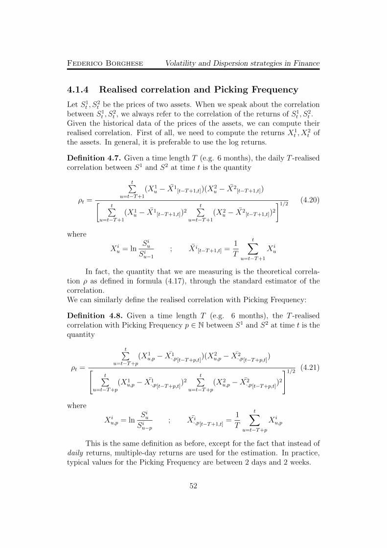
4.1.4 Realised correlation and Picking Frequency
Let S1t , S
2t be the prices of two assets. When we speak about the correlation
between S1t , S
2t , we always refer to the correlation of the returns of S1
t , S2t .
Given the historical data of the prices of the assets, we can compute theirrealised correlation. First of all, we need to compute the returns X1
t , X2t of
the assets. In general, it is preferable to use the log returns.
Definition 4.7. Given a time length T (e.g. 6 months), the daily T -realisedcorrelation between S1 and S2 at time t is the quantity
ρt =
t∑u=t−T+1
(X1u − X1
[t−T+1,t])(X2u − X2
[t−T+1,t])[t∑
u=t−T+1
(X1u − X1
[t−T+1,t])2t∑
u=t−T+1
(X2u − X2
[t−T+1,t])2
]1/2(4.20)
where
X iu = ln
SiuSiu−1
; X i[t−T+1,t] =
1
T
t∑u=t−T+1
X iu
In fact, the quantity that we are measuring is the theoretical correla-tion ρ as defined in formula (4.17), through the standard estimator of thecorrelation.We can similarly define the realised correlation with Picking Frequency:
Definition 4.8. Given a time length T (e.g. 6 months), the T -realisedcorrelation with Picking Frequency p ∈ N between S1 and S2 at time t is thequantity
ρt =
t∑u=t−T+p
(X1u,p − X1
·,p[t−T+p,t])(X2
u,p − X2·,p[t−T+p,t]
)[t∑
u=t−T+p
(X1u,p − X1
·,p[t−T+p,t])2
t∑u=t−T+p
(X2u,p − X2
·,p[t−T+p,t])2
]1/2(4.21)
where
X iu,p = ln
SiuSiu−p
; X i·,p[t−T+1,t]
=1
T
t∑u=t−T+p
X iu,p
This is the same definition as before, except for the fact that instead ofdaily returns, multiple-day returns are used for the estimation. In practice,typical values for the Picking Frequency are between 2 days and 2 weeks.
52

Federico Borghese Volatility and Dispersion strategies in Finance
The Picking Frequency correlation still estimates correlation
The above defined estimator is still measuring the correlation between X1u,p =
ln S1u
S1u−p
and X2u,p = ln S2
u
S2u−p
. We have
X iu,p = ln
SiuSiu−p
=u∑
v=u−p+1
lnSivSiv−1
=u∑
v=u−p+1
X iv
Under the Black-Scholes model, the X iv are i.i.d. N(0, σ2
i /252), hence X iu,p ∼
N(0, p252σ2x). The covariance between X1
u,p and X2u,p is
E[X1u,pX
2u,p
]= E
[(u∑
v=u−p+1
X1v
)(u∑
v=u−p+1
X2v
)]=
=u∑
v=u−p+1
E[X1vX
2v
]= pρσ1σ2/252
(4.22)
In the previous steps, mixed terms disappear because returns in differentdays are independent. Therefore the correlation between X1
u,p and X2u,p is
the same ρ as it is with daily returns.
Why using Picking Frequencies
In the formula (4.20), daily log returns are used as a statistical sample forcomputing the estimator (4.2). Daily returns means specifically close to closereturns, i.e. the price used for every day is the price fixing at the close ofthe exchange where the asset is traded. Using daily returns therefore isappropriate only if the two assets are traded in the same geographical area:we require that the 2 prices at the close are synchronous.This is not the case when measuring, for example, the correlation betweenthe EuroStoxx 50 and the S&P 500: markets opening hours are far fromsynchronous in Europe and in the US. As can be seen in figure 4.2, usingthe daily returns we mistakenly use asynchronous returns in the estimation,thus underestimating the true correlation between the assets.
Theorem 4.9. Suppose that At and Bt are the prices of two assets. AssumeBlack-Scholes dynamics for the two assets, with a correlation of ρ (defined asin section 4.1.3). Let 0 < α < 1 be a real number, representing a lag betweenclosing hours of the exchanges where A and B are traded, less than 1 daylong. Let ρp,α be the correlation between the close-to-close p-days returns ofA and B. To be precise,
ρp,α = Correl
(ln
AtAt−p
, lnBt+α
Bt−p+α
)(4.23)
53
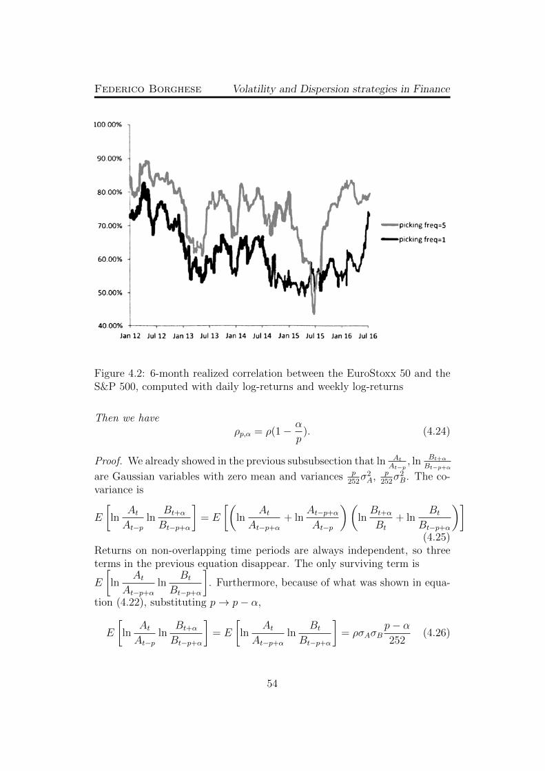
Federico Borghese Volatility and Dispersion strategies in Finance
Figure 4.2: 6-month realized correlation between the EuroStoxx 50 and theS&P 500, computed with daily log-returns and weekly log-returns
Then we haveρp,α = ρ(1− α
p). (4.24)
Proof. We already showed in the previous subsubsection that ln AtAt−p
, ln Bt+αBt−p+α
are Gaussian variables with zero mean and variances p252σ2A, p
252σ2B. The co-
variance is
E
[ln
AtAt−p
lnBt+α
Bt−p+α
]= E
[(ln
AtAt−p+α
+ lnAt−p+αAt−p
)(lnBt+α
Bt
+ lnBt
Bt−p+α
)](4.25)
Returns on non-overlapping time periods are always independent, so threeterms in the previous equation disappear. The only surviving term is
E
[ln
AtAt−p+α
lnBt
Bt−p+α
]. Furthermore, because of what was shown in equa-
tion (4.22), substituting p→ p− α,
E
[ln
AtAt−p
lnBt+α
Bt−p+α
]= E
[ln
AtAt−p+α
lnBt
Bt−p+α
]= ρσAσB
p− α252
(4.26)
54
Federico Borghese Volatility and Dispersion strategies in Finance
Finally, we compute
ρp,α =ρσAσB(p− α)√
pσ2A · pσ2
B
= ρ
(1− α
p
)(4.27)
Thanks to the previous theorem, we now see why a daily (p = 1) corre-lation underestimates the true correlation when working with the Europeanand American stocks. We also observe that
The higher the Picking Frequency p, the smaller is the underesti-mation error made on the correlation.
However, correlation is a variable quantity, so an excessively big PickingFrequency fails to capture the instantaneous correlation. Acceptable valuesfor the Picking Frequency are in the range 3 to 10 days.
4.2 Correlation of n > 2 assets
All the definitions for correlation given so far only apply to a pair of randomvariables. We want to generalise this concept for n > 2 random variables.In mathematics there is the concept of copulas to describe multi-dimensionaldependence between random variables. However, copulas are complicatedobjects (they are functions), whereas we are looking for a single real numberto describe the dependence.It is clear that 3 variables which have pairwise correlations equal to 1 willhave a “threewise” correlation equal to 1. However, if the variables areX1 = X,X2 = X,X3 = −X, the correlations will be +1,−1,−1. Now themeaning of a “threewise” correlation is less clear.Let us set up the problem within the financial framework: we have S1
t , ..., Snt
the prices of n stocks. The daily returns of the stocks are∆SitSit
=Sit+1
Sit− 1. In
what follows, in order for the correlation to have a meaningful sense, we willmake the following assumption:
Assumption 4.10. For every pair Si, Sj of assets, let ρi,j be the Pearsoncorrelation between the two stocks. From now on, we assume that ρi,j ≥ 0for every i, j and that the values of the ρi,j are all close to each other (say,no more than 50% difference in any pair of correlations).
55

Federico Borghese Volatility and Dispersion strategies in Finance
This assumption is reasonable when working with equities: usually theconsidered assets are stocks in the same sector or in the same country andhave positive, similar correlations between pairs.
4.2.1 Average Pairwise Correlation
A possible way to define the realised correlation between the n assets is tosimply take the average of the 1
2n(n− 1) pairwise realised correlations. That
is
ρ =2
n(n− 1)
∑i 6=j
ρij (4.28)
The above definition needs assumption 4.10 to make sense. For example, inthe case of 3 assets with S2 = S1, S3 = −S1, the above formula would yielda correlation of −1
3which is hard to interpret. But if the correlations were
50%, 60%, 55% (these are typical values), a value of 55% for the three-wisecorrelation is acceptable and has a good interpretation.
4.2.2 Clean and Dirty Correlations
These definitions of correlation are the ones which naturally appear in dis-persion strategies, which we will study in the next chapter.Take S1
t , ..., Snt the prices of n assets. Let B be a dynamic basket of the
stocks,as defined in equation (2.16), with constant weights w1, ...wn. As-suming that the daily returns of the assets have a stationary distributionwith mean 0 and variances σ2
1/252, ..., σ2n/252, we can compute the volatility
of the basket as follows:
σ2B = 252V ar
[∆B
B
]= 252V ar
[n∑i=1
wi∆Si
Si
]=
=n∑i=1
(wi)2σ2i + 2
∑i<j
wiwjσiσjρij
(4.29)
Assuming that all the correlations are equal, i.e. ρij = ρ, the above formulabecomes
σ2B =
n∑i=1
(wi)2σ2i + 2ρ
∑i<j
wiwjσiσj = (4.30)
=n∑i=1
(wi)2σ2i + ρ
( n∑i=1
wiσi
)2
−n∑i=1
(wi)2σ2i
= (4.31)
56

Federico Borghese Volatility and Dispersion strategies in Finance
= ρ
(n∑i=1
wiσi
)2
+ (1− ρ)n∑i=1
(wi)2σ2i (4.32)
From the above relations we can derive two possible definitions for the n-dimensional correlation. The first one is obtained by deriving ρ from theequation (4.31):
Definition 4.11. The implied/realised clean correlation among the n assetsis defined as
ρ =σ2B −
∑ni=1(wi)2σ2
i
(∑n
i=1wiσi)
2 −∑n
i=1(wi)2σ2i
(4.33)
where σB, σi are the implied/realized volatilities of the basket and the i-thasset.
In the case that the number of assets is sufficiently large and the weightsare not far from equal weights, there is a handy approximation. In equation(4.32), the order of magnitude of the first term is(
n∑i=1
wiσi
)2
≈
(n∑i=1
1
nσ
)2
= σ2 (4.34)
The second term instead is
n∑i=1
(wi)2σ2i ≈
n∑i=1
1
n2σ2 =
1
nσ2 (4.35)
We clearly see that for n large enough, say 50 stocks as the number of com-ponents of the EuroStoxx 50, the second term is only 2% of the first term.Therefore it is a not too bad approximation to drop it. Hence we find
σ2B ≈ ρ
(n∑i=1
wiσi
)2
(4.36)
Definition 4.12. The implied/realised dirty correlation among the n assetsis defined as
ρ =
σBn∑i=1
wiσi
2
(4.37)
where σB, σi are the implied/realized volatilities of the basket and the i-thasset.
57
Federico Borghese Volatility and Dispersion strategies in Finance
Observation 4.13. The dirty correlation is always larger than the cleancorrelation. From equation (4.32) we see that σ2
B ≥ ρclean (∑n
i=1wiσi)
2and
the conclusion follows.
Observation 4.14. Whereas it is not possible to define an implied averagepairwise correlation, it becomes possible to define implied clean/dirty cor-relations, provided that there are liquid options on the basket and on theunderlyings.
Realized volatility of the basket
Special attention must be made when computing the realized volatility ofa basket. If all the basket components are traded in the same hours, therealized volatility can be normally computed with the daily close-to-closelog-returns of the basket. However, if the basket components are traded indifferent geographical areas, the volatility of the basket must be computedwith a Picking Frequency (e.q. 3-5 days). Otherwise the time lag introducesa decorrelation among the assets and therefore reduces the volatility of thebasket.
58

Chapter 5
Dispersion
5.1 Interest in trading correlation
Investment banks keep on selling structured products containing Worst-Offeatures, options on Baskets and many more sophisticated payoffs with along exposure to correlation. On the other hand, institutional investors keepon buying Puts on indices for protection; portfolio managers keep on sellingvolatility on single stocks, typically through call overwriting to enhance theirperformance. The effect is that single stock volatility is relatively cheap andindex volatility is relatively expensive. The combined behaviours of the buyside and the sell side create a spread between implied and realised correlation(which empirically is around 10 points). Investment banks find themselveswith big short exposure to correlation and want to buy correlation back; onthe buy side, many clients want to profit from the attractive returns offeredby a short correlation exposure.A possible way to directly trade correlation is Correlation Swaps. These in-struments are simply forward contracts on the Pairwise Realised Correlation.However they are not very liquid, and there is no method to define an impliedpairwise correlation. Also, there are obvious hedging problems: correlationis a very elusive quantity which is difficult to replicate with other financialproducts. From these reasons comes the popularity of Dispersion Trades,which provide an exposure to correlation but also benefit from the liquidityof options, they are easy to implement and easy to hedge.
59

Federico Borghese Volatility and Dispersion strategies in Finance
5.2 General Dispersion Trade
Dispersion Trades consist in taking a position in an index option and takingthe opposite position in all the index components. Let Bt be the spot price ofan Equity Index (say, the EuroStoxx 50), and S1, ..., Sn be the spot prices ofthe n Index components. We can assume by normalization that S1
0 = S20 =
... = Sn0 = B0 = 1. Let w1, ..., wn be the weights of the components, andα1, ..., αn be positive real numbers (not necessarily with unit sum). Let O(·)be a generic derivative product (e.g. a Call, a Put, a Straddle, a VarianceSwap).
Definition 5.1. A Dispersion Trade “O VS O” (e.g. Call VS Call, StraddleVS Straddle etc.) on the index B with weights α1, ..., αn consists in being
• Long αi options O on the i-th component on the index
• Short 1 option O on the Index
In formulas,
Disp =n∑i=1
αiO(Si) −O(B) (5.1)
Suppose that the product O has a positive vega (which is the casefor Calls, Puts, Straddles and Variance Swaps). A Dispersion trade is thusbuying volatility on the single stocks and selling volatility on the basket.Since the volatility of the basket is an increasing function of the correlation,the Dispersion Trade is short correlation. In general, Dispersion Tradesare Delta Hedged, in order to remove the directional exposure and only keepthe volatility and correlation exposure.
Proposition 5.2. If the option O is a European payoff which is a convexfunction of the underlying price (true for Calls, Puts, Straddles), the basketB is an arithmetic basket of the underlyings and αi = wi, then the Dispersionpayoff is always positive.
Proof. By hypothesis, O(Si) = f(SiT ) with f being a convex function. B isan arithmetic basket, i.e. BT =
∑ni=1wiS
iT . By Jensen’s inequality,
n∑i=1
wif(SiT ) ≥ f
(n∑i=1
wiSiT
)= f(BT )
60

Federico Borghese Volatility and Dispersion strategies in Finance
5.3 Gamma P&L
Having said that the Dispersion trades are often Delta-Hedged, it is interest-ing to investigate the Gamma P&L of being long the dispersion strategy.Throughout this section, we assume that the Basket is a dynamic Basketwith weights wi, as defined in section 2.4. For the case of a static Basketwith weights wi, it is sufficient to substitute
wi =wiSiB
(5.2)
In any case, we have that the sum of the weights is one.Let Γ1, ...Γn,ΓB be the Gammas of the option O on the single stocks andon the Basket (assumed to be all positive), and σ1, ...σn, σB the volatilities.Reminding equation (2.15), we can write the Gamma P&L of the Dispersiontrade:
P&LΓ = −n∑i=1
1
2αiΓiS
2i
(σ2i ∆t−
(∆SiSi
)2)
+1
2ΓBB
2
(σ2B∆t−
(∆B
B
)2)
(5.3)
Set σ2i ∆t :=
(∆SiSi
)2
and σ2B∆t :=
(∆BB
)2. To clarify, σi and σB can be seen as
instantaneous realized volatilities. Using the clean correlation as describedin definition 4.11, with ρ being the implied and ρ being the one-day realised,we can rewrite
σ2B −
1
∆t
(∆B
B
)2
= σ2B − σ2
B =∑
w2i σ
2i + ρ
[(∑wiσi
)2
−∑
w2i σ
2i
]−
−∑
w2i σ
2i − ρ
[(∑wiσi
)2
−∑
w2i σ
2i
](5.4)
61

Federico Borghese Volatility and Dispersion strategies in Finance
Now we can combine the two previous equations, putting together the σ2i −σ2
i
terms:
Dispersion Gamma P&L with clean correlation - dynamic Basket
2
∆tP&LΓ =
n∑i=1
(σ2i − σ2
i
) [αiΓiS
2i − ΓBB
2w2i
]+
+ ΓBB2
{ρ
[(∑wiσi
)2
−∑
w2i σ
2i
]− ρ
[(∑wiσi
)2
−∑
w2i σ
2i
]}Dispersion Gamma P&L with clean correlation - static Basket
2
∆tP&LΓ =
n∑i=1
(σ2i − σ2
i
)S2i
[αiΓi − ΓBw
2i
]+
+ΓB
{ρ
[(∑wiSiσi
)2
−∑
w2i S
2i σ
2i
]− ρ
[(∑wiSiσi
)2
−∑
w2i S
2i σ
2i
]}(5.5)
In the case of the number of stocks n being sufficiently large, and the weightssufficiently balanced, we can make an approximation dropping the terms inw2i and thus using the dirty correlations, obtaining
Dispersion Gamma P&L with dirty correlation - dynamic Basket
2
∆tP&LΓ =
n∑i=1
(σ2i − σ2
i
)αiΓiS
2i + ΓBB
2
{ρ(∑
wiσi
)2
− ρ(∑
wiσi
)2}
(5.6)where ρ is now the dirty correlation. The above P&L can be interpretedas a first long exposure in single-stock volatility and a second shortexposure to covariance (not correlation). In order to identify the pureexposure to correlation, we can rewrite it as
2
∆tP&LΓ =
n∑i=1
(σ2i − σ2
i
)αiΓiS
2i + ΓBB
2ρ
[(∑wiσi
)2
−(∑
wiσi
)2]
+
+ ΓBB2(∑
wiσi
)2
(ρ− ρ)
(5.7)
or also
2
∆tP&LΓ =
n∑i=1
(σ2i − σ2
i
)αiΓiS
2i + ΓBB
2ρ
[(∑wiσi
)2
−(∑
wiσi
)2]
+
+ ΓBB2(∑
wiσi
)2
(ρ− ρ)
(5.8)
62

Federico Borghese Volatility and Dispersion strategies in Finance
For a rough interpretation of the previous equations, we can imagine all theσi to equal to a common “single-stock volatility” σ. We have
Dispersion Gamma P&L simplified to highlight the exposure tosingle-stock volatility and correlation
2
∆tP&LΓ =
(σ2 − σ2
) [ n∑i=1
αiΓiS2i − ρΓBB
2
]+ ΓBB
2σ2(ρ− ρ) (5.9)
Dispersion Gamma P&L simplified to highlight the exposure to single-stock volatility and covariance
2
∆tP&LΓ =
(σ2 − σ2
) [ n∑i=1
αiΓiS2i − ρΓBB
2
]+ ΓBB
2σ2(ρ− ρ) =
=(σ2 − σ2
) [ n∑i=1
αiΓiS2i
]+ ΓBB
2(σ2ρ− σ2ρ
)(5.10)
5.4 Examples of Dispersion Strategies
5.4.1 Variance Swap VS Variance Swap Dispersion
The most classical example of a Dispersion Strategy consists in buying aVariance Swap with Vega Notional Ni on the i-th component of the indexand selling a Variance Swap with Vega Notional NB on the Basket.Let Ki, σ
2i be the Variance Swap strike and Realised Variance of the i-th
component and KB, σ2B the Variance Swap strike and Realised Variance of
the Basket. The payoff of the trade is simply
Disp =n∑i=1
Niσ2i −K2
i
2Ki
−NBσ2B −K2
B
2KB
(5.11)
Set αi = Ni2Ki
and αB = NB2KB
; the payoff is then
Disp =n∑i=1
αi(σ2i −K2
i
)− αB
(σ2B −K2
B
)(5.12)
63
Federico Borghese Volatility and Dispersion strategies in Finance
Let ρij be the realised correlation between assets i, j; we have, similarly toequation (4.29),
σ2B =
n∑i=1
w2i σ
2i + 2
∑i<j
wiwjσiσj ρij (5.13)
We can see the strikes Ki, KB as implied volatilities, and define the ImpliedCorrelations ρij. We have that
K2B =
n∑i=1
w2iK
2i + 2
∑i<j
wiwjKiKjρij (5.14)
Therefore,
Disp =n∑i=1
(αi − αBw2
i
) (σ2i −K2
i
)− 2αB
∑i<j
wiwj (σiσj ρij −KiKjρij)
(5.15)
We can see the above payoff as a combination of a long volatility ex-posure on single stocks and a short covariance (not correlation) exposureσiσj ρij −KiKjρij.In the case of the number of stocks being high, we can use the Dirty Corre-lations ρ, ρ (realised, implied) as defined in definition 4.12. From (5.12) wesee that
Disp =n∑i=1
αi(σ2i −K2
i
)− αB
ρ( n∑i=1
wiσi
)2
− ρ
(n∑i=1
wiKi
)2 (5.16)
The sensitivity to the volatility of the j-th component is
∂Disp
∂σj= 2αjσj − 2αBwj ρ
n∑i=1
wiσi (5.17)
Assuming that all σi are the same, we have that the Vega of the Dispersionis
∂Disp
∂σ= 2(
n∑j=1
αj − αBρ)σ (5.18)
Weightings
There are many interesting weighting choices of the αi.
64

Federico Borghese Volatility and Dispersion strategies in Finance
Covariance Dispersion (in case of a small number of stocks) Inorder to have an as pure as possible exposure to covariance, we see fromequation (5.15) that we must choose αi = αBw
2i . This is suitable when the
number of stocks is small; when there are many stocks, this weighting choicebecomes equivalent to just selling a Variance Swap on the Basket. The payoffin this case will be
Disp = −2αB∑i<j
wiwj (σiσj ρij −KiKjρij) (5.19)
Correlation Weighted Dispersion The aim of this weighting is to beVega Neutral, that is eliminating the exposure to volatility and only keepingthe correlation exposure. From equation (5.17) and (5.18), we see that thebest choice is αi = αBwiρ (hence the name Correlation Weighted). Actually,since ρ is unknown, a forecast value will be used.
Vega Weighted Dispersion The weights are αi = wiαB, or alternativelyNi = 2wiKi, NB = 2KB (hence the name Vega Weighted). This choice can beseen as a Correlation Weighted dispersion plus a long position in single-stockvolatility:
Vega Weighted =n∑j=1
αBwj(1− ρ)(σ2i −K2
i
)+ Correlation Weighted
The rationale is in the fact that correlation and volatility are positively cor-related. Therefore a long position in single-stock volatility reduces the lossesof the short correlation exposure when both volatility and correlation rise.
5.4.2 Synthetic Variance Swap Dispersion
Very similar to the Variance Swap Dispersion is buying αi synthetic VarianceSwaps1 on the i-th component of the index and selling a synthetic VarianceSwap on the Index.As we saw in equation (3.21), the Gamma of the portfolio which replicates aVariance Swap is Γ = 2
TS2t. So, by equation (5.9), we have
P&LΓ =∆t
T
[(σ2 − σ2
)( n∑i=1
αi − ρ
)+ σ2(ρ− ρ)
](5.20)
1A Synthetic Variance Swap consists in buying the replicating portfolio defined in (3.14)and Delta-Hedging it.
65

Federico Borghese Volatility and Dispersion strategies in Finance
The P&L is in line with the case of the Variance Swap Dispersion. With theweighting choice Correlation Weighted αi = wiρ,
∑ni=1 αi = ρ and the P&L
becomes
P&LΓ =∆t
Tσ2(ρ− ρ) (5.21)
As in the case of the Variance Swap, the Correlation Weighted Dispersionprovides a rather pure exposure to correlation.The Vega Weighted Dispersion αi = wi produces a P&L of
P&LΓ =∆t
T
[(σ2 − σ2
)(1− ρ) + σ2(ρ− ρ)
](5.22)
We again see it as a Correlation Weighted Dispersion plus a long position insingle-stock volatility, which can mitigate losses when correlation and vola-tility surge together.
5.4.3 ATM Call VS Call Dispersion
It consists in buying αi ATM European Calls on the i-th component of theindex and selling an ATM Call on the Index, and Delta Hedging every option.Because of the liquidity of Call Options, this strategy is attractive, easy toimplement and easy to hedge.The Gamma of a Call Option in Black-Scholes model is
Γ =Φ(d+)
Stσ√T − t
where σ is the volatility, Φ(x) = e−x2/2/√
2π is the density function of thestandard Gaussian and
d+ =
[ln St
K+(r + 1
2σ2(T − t)
)]σ√T − t
At inception we can say that Φ(d+) is roughly the same value for all thestocks and the Basket, being all the prices equal to the strike. Recall thatσB = σ
√ρ with ρ being the dirty correlation, and prices at inception are all
equal to 1. Then, by equation (5.10), we have
2
∆tP&LΓ =
Φ(d+)√T
{(σ2 − σ2
) [ n∑i=1
αiSiσ− ρ B
σB
]+B
σBσ2(ρ− ρ)
}=
=Φ(d+)
σ√T
{(σ2 − σ2
) [ n∑i=1
αi −√ρ
]+ σ2ρ− ρ√
ρ
}(at inception)
(5.23)
66

Federico Borghese Volatility and Dispersion strategies in Finance
From the above formula, we see that the Correlation Weighted Dispersion isobtained with weight choices such that
∑αi =
√ρ. However, there is a big
problem in the above strategy. The Gamma of a Call Option is maximisednear the strike and rapidly decreases when the spot moves away. This effectis expressed in the above formula in the Φ(d+) term, where the Gaussianbell appears. Therefore, when spots move away from the ATM over time,the Gamma vanishes and what is captured on only noise. The strategy maybe good for short maturities (e.g. 6 months) because the spots don’t havemuch time to move away from the ATM, but for longer maturities it doesnot capture anymore the correlation.
Table 5.1: Pros and Cons of ATM Call VS Call
Pros Cons
Uses liquid instruments
Provides exposure to correlation
Easy to hedge
When spots move away from the ATM,Gamma vanishes and the P&L is noise
5.4.4 Straddle VS Straddle or Put VS Put
The P&Ls of a Call Delta Hedged and of a Put Delta Hedged with samestrike are equal. This can be justified by the Call-Put parity or by the factthat the Gamma of a Call is equal to the Gamma of a Put with the samestrike. Therefore, provided that the Dispersion strategy is Delta Hedged,using Calls, Puts or Straddles gives the same outcome. There could be someinterest in using Straddles because of their smaller delta at inception.
5.4.5 Call Strip VS Call Strip
The aim of this strategy is to deal with the vanishing Gamma issue of theATM Call VS Call Dispersion while providing the same advantages describedin table 5.1. A possible solution is to use multiple vanilla options with dif-ferent strikes in order to keep the Gamma significantly high for a wider spotrange.Using too many vanillas with the widest range of strikes has the major in-convenience of delta-hedging too many options. For example, if we use 10options and our dispersion runs on 50 components, we need to delta-hedge10× (50 + 1) = 510 options.There are many possibilities in the choice of the weightings. One choice is,
67

Federico Borghese Volatility and Dispersion strategies in Finance
recalling the replication of a Variance Swap, to use weights proportional tothe inverse square strike 1/K2.Let us choose weights such that
∑αi =
√ρ (Correlation Weighted). Assum-
ing that the Gamma does not vanish, we see from equation (5.23) that theP&L is proportional to:
P&LΓ ∝ B · σ2
σ· ρ− ρ√
ρ≈ σ(
√ρ−
√ρ) (5.24)
5.5 Backtest
We took an arithmetic basket of 10 stocks, whose tickers will not be disclosedfor confidentiality reasons. The implied 6-month correlation of the 10 com-ponents has been around 50−60% in the past 5 years. The realised 6-monthcorrelation has almost always been below 50%, as expected (we said thatusually the realised correlation is 5-10 points below the implied correlation).We chose to backtest a Correlation Weighted Dispersion with three 6-monthvanilla options, with strikes 90%, 100%, 110%. Being the implied correla-tion around 50 − 60%, it seems reasonable to take weightings such that∑αi ≈
√ρ ≈ 80%. The complete strategy is therefore
Disp = 80%× 1
10
10∑i=1
∑K∈{90%,100%,110%}
1
K2V anilla(K,SiT )
−−
∑K∈{90%,100%,110%}
1
K2V anilla(K,BT )
+ DeltaHedge− Premium
(5.25)
In the above equation, V anilla(K,SiT ) is either a Call or a Put option struckat K on the i-th underlying. It does not matter whether it is a Call or a Putbecause the whole strategy is Delta Hedged. As can be seen in figure 5.1,the P&L of the strategy is short correlation. Moreover, the approximationin equation (5.24) manages to well describe the P&L, as shown in figure 5.2.
68

Federico Borghese Volatility and Dispersion strategies in Finance
Figure 5.1: P&L of the Dispersion Strategy compared to 6-month realisedcorrelation.
Figure 5.2: P&L of the Dispersion Strategy compared to f(ρ) = σ(√
50%−√ρ. In the formula, ρ is the 6-month realised correlation and σ is the average
of the 6-month realised volatilities of the 10 stocks.
69

Chapter 6
Some new ideas
The job of a Structurer also includes the creation of new, innovative products.In my opinion, this is one of the best aspects of the job: the stimulatingatmosphere in the team and the outstanding skills of the colleagues spurcreativity and curiosity. In this brief chapter I show two of my new ideas.
6.1 Putting together Dispersion and Variance
Replication: The Gamma Covariance Swap
In this section we put together the ideas developed in the replication ofWeighted Variance Swaps (subsection 3.3.3) and the Call VS Call Disper-sion. The result will provide a robust replication of the Realised “GammaCovariance”, a quantity that, as far as I know, did not exist before. I chosethis name because of the analogy with the Gamma Swap.
Definition 6.1. Let At, Bt be the prices of two assets, with volatilities σAt , σBt
and correlation ρt. The Gamma Covariance between At, Bt on the period[0, T ] is the following quantity:
ΓCov =252
T
∫ T
0
AtA0
· Bt
B0
ρtσAt σ
Bt dt (6.1)
The Realised Gamma Covariance is:
ΓCov =252
T
T∑t=1
At−1
A0
· Bt−1
B0
log
(AtAt−1
)log
(Bt
Bt−1
)(6.2)
The Gamma Covariance differs from the Covariance in the fact thatthe log-returns are weighted by the spot. The Gamma Covariance’s relation
70

Federico Borghese Volatility and Dispersion strategies in Finance
with Covariance is in a close analogy with the Gamma Swap’s relation withthe Variance Swap, because in Gamma Swaps the squared log-returns arespot-weighted.In order to understand the key features of the Gamma Swap and of theGamma Covariance, we should keep in mind the following empirical result:
Market Fact: Let At, Bt be the prices of two Equities, with volatil-ities σAt , σ
Bt and correlation ρt. The following events usually happen either
all together or none at all:
1. Both the spots At, Bt go down;
2. Both the volatilities σAt , σBt go up;
3. The correlation ρt goes up.
Observation 6.2. The effect of the weighting by the spot is very similarto the mitigating effect produced by the Gamma Swap. In normal marketconditions (where the spots don’t move too much away from their initialvalue), the Gamma Covariance is almost identical to the Covariance (exactlyas the Gamma Swap is almost identical to the Variance Swap). In adversemarket conditions, the covariance explodes: by the above Market Fact, allthe three factors of the covariance=ρtσ
At σ
Bt surge together. In contrast, the
Gamma Covariance Swap does not explode, thanks to the mitigating effectof weighting by the spots, which are usually down in the same scenario.
6.1.1 Replication
The above observations make it clear that a Gamma Covariance Swap willhave a cheaper strike than a standard Covariance Swap (as the Gamma Swapstrike is cheaper than the Variance Swap strike). Another main interest ofa Gamma Covariance Swap is the possibility to perfectly replicate it in thefollowing manner:
Theorem 6.3. The Gamma Covariance is replicable with delta strategies inthe Underlyings, a zero-coupon Bond, forwards and Call VS Call (or PutVS Put) dispersions with weights
(14, 1
4
)on the single stocks and −1 on the
71

Federico Borghese Volatility and Dispersion strategies in Finance
basket. In formulas,
ΓCov =1
T
[−2 + 2
(ATA0
+ BTB0
2
)− 1
B0
∫ T
0
AtA0
dBt −1
A0
∫ T
0
Bt
B0
dAt−
− 4
∫ +∞
0
[1
4V anK
(ATA0
)+
1
4V anK
(BT
B0
)− V anK
(ATA0
+ BTB0
2
)]dK
](6.3)
where V anK(x) is the payoff of the Vanilla Call/Put on x struck at K whichwas Out-Of-The-Money at inception, i.e.
V anK(x) =
{(x−K)+ if K > 1
(K − x)+ if K < 1(6.4)
Proof. Throughout the proof, let us assume by normalization that A0 =B0 = 1.Step 1: Ito’s formula. By applying Ito’s formula to the function f(x, y) =xy, we have
ATBT − A0B0 =
∫ T
0
AtdBt +
∫ T
0
BtdAt +
∫ T
0
AtBtρtσAt σ
Bt dt (6.5)
ΓCov =1
T
[ATBT − 1−
∫ T
0
AtdBt −∫ T
0
BtdAt
](6.6)
We now see that, in order to replicate the Gamma Covariance, apart from im-plementing delta strategies, we need to replicate the European payoff ATBT .Carr’s formula can’t help us now, as it works only on a European payoff ona single underlying.Step 2: Algebra trick.
ATBT = 2
(AT +BT
2
)2
− 1
2A2T −
1
2B2T (6.7)
With the above trick we decompose the payoff ATBT as a sum of payoffs onA,B and on the basket AT+BT
2.
Step 3: Carr’s formula. By Carr’s formula (2.1) applied three times,with S∗ = 1, we have:
2
(AT +BT
2
)2
= 2 + 4
(AT +BT
2− 1
)+ 4
∫ +∞
0
V anK
(AT +BT
2
)dK
(6.8)
72

Federico Borghese Volatility and Dispersion strategies in Finance
− 1
2A2T = −1
2− (AT − 1)−
∫ +∞
0
V anK (AT ) dK (6.9)
− 1
2B2T = −1
2− (BT − 1)−
∫ +∞
0
V anK (BT ) dK (6.10)
Step 4: Combine the first 3 steps. By summing the last three equa-tions we obtain:
ATBT = −1 + 2
(AT +BT
2
)−
− 4
∫ +∞
0
[1
4V anK (AT ) +
1
4V anK (BT )− V anK
(AT +BT
2
)]dK
(6.11)
Plugging the replication of the payoff ATBT into equation (6.6) we find thethesis.
Observation 6.4. With the same procedure, we might want to replicate the(not Gamma) covariance as well. However, this is not possible with the samemethod. We would need to apply Ito’s formula to a function G(A,B) suchthat
∂2G
∂A∂B=
1
AB;
∂2G
∂A2=∂2G
∂B2= 0 (6.12)
Unfortunately, such a function does not exist.
6.1.2 Backtest
We have backtested the results in this section on the EuroStoxx 50 and theFTSE 100 (we chose this pair because they trade in the same market hours),as well as on an Equity Basket composed of 7 stocks. The backtests confirmedthat
• The Gamma Covariance does not explode in the 2008 financial crisisand after the dot-com bubble (whereas the covariance does);
• The Gamma Covariance is the same as Covariance except during mar-ket stress.
• The 1-year realised Gamma Covariance is perfectly replicated by thestrategy described in equation (6.3). The strategy is implemented withdaily rebalanced delta strategies, and a strip of Vanilla options to repro-duce the integral. We chose strikes ranging from 40% to 160%, evenlyspaced by 5 points. For the ATM Dispersion, we used one half of theATM Call VS Call and one half of the ATM Put VS Put.
73

Federico Borghese Volatility and Dispersion strategies in Finance
Figure 6.1: Comparison between 1-year realised Covariance and GammaCovariance between the EuroStoxx 50 and the FTSE 100. The two quantitiesare almost the same in normal market conditions, but selling the GammaCovariance brings about mitigated losses during market crashes compared toselling the Covariance.
Figure 6.2: Spread between 1-year realised Covariance and Gamma Covari-ance between the EuroStoxx 50 and the FTSE 100.
74

Federico Borghese Volatility and Dispersion strategies in Finance
Figure 6.3: 1-year realised Gamma Covariance between the EuroStoxx 50 andthe FTSE 100, and its replication according to Theorem 6.3. The replicationmakes use of strikes ranging from 40% to 160%, evenly spaced by 5%. Thereplication is almost perfect, having a replication error of 3 basis points onaverage.
75

Federico Borghese Volatility and Dispersion strategies in Finance
Figure 6.4: Comparison between 1-year realised Covariance and GammaCovariance in the case of a Basket of 7 stocks. The two measures are theweighted averages of the 21 Covariances and Gamma Covariances betweeneach pair of stocks. The weights are proportional to the inverse of volatilitiesat inception, so the quantities can be somehow identified with correlations(despite being larger than 1 when both correlation and volatility surged in2008).
76

Federico Borghese Volatility and Dispersion strategies in Finance
6.2 The FX-Gamma Covariance
The previous section is valid regardless of the asset classes of the underlying;nevertheless, it is designed and thought for two Equities. In this sectionI present a slightly different definition of the Gamma Covariance which isadapted to an Equity Index and a FX rate.Let £ be a foreign currency and $ be a domestic currency (in this examplewe imagine to be a US investor looking at the British Equity market, butit could be any pair of currencies). Let St be the price in £ of a foreignshare, and Xt be the GBP/USD exchange rate (to be precise, Xt is the valuein dollars of £1). Suppose that an American Depositary Receipt on S istradable in the US market, with price ADRt = StXt.
Definition 6.5. The FX-Gamma Covariance between the foreign asset Stand the FX rate Xt on the period [0, T ] is defined as
FXΓ =252
T
T∑t=1
St−1
S0
log
(StSt−1
)log
(Xt
Xt−1
)(6.13)
or, in the continuous world,
FXΓ =252
T
∫ T
0
StS0
σSt σXt ρ
SXt dt (6.14)
where σSt σXt ρ
SXt is the covariance between S and X. Alternatively, returns
could be computed with a Picking Frequency to compensate for the differencein trading hours between the two markets.
6.2.1 Replication
The FX-Gamma Covariance is very similar to the normal covariance. If wespeak about an Equity and a FX rate, the covariance can be positive ornegative, and tends to reach extremal values when the Equity crashes. Theeffect of multiplying by the price in the FX-Gamma Covariance mitigates thiseffect, and most importantly makes that quantity perfectly replicable.
77

Federico Borghese Volatility and Dispersion strategies in Finance
Theorem 6.6. The FX-Gamma Covariance is replicable with the fol-lowing instruments: a Quanto Forward on the foreign Equity, a Deltastrategy in the ADR and a Delta Strategy on the FX rate. In formulas,
FXΓ =252
T
[−(STS0
− 1
)+
1
S0
T∑t=1
1
Xt−1
(ADRt − ADRt−1)−
− 1
S0
T∑t=1
St−1
Xt−1
(Xt −Xt−1)
] (6.15)
Proof. Let us assume the following general diffusion model:{dStSt
= µSt dt+ σSt dWSt
dXtXt
= µXt dt+ σXt dWXt
(6.16)
with d[W St ,W
Xt ] = ρSXt dt. By Ito’s formula,
dADRt = d(StXt) = XtdSt + StdXt + StXtσSt σ
Xt ρ
SXt dt (6.17)
Therefore, by dividing by Xt, we obtain
1
Xt
dADRt = dSt +StXt
dXt + StσSt σ
Xt ρ
SXt dt (6.18)
and integrating both sides provides∫ T
0
1
Xt
dADRt = (ST − S0) +
∫ T
0
StXt
dXt +T
252FXΓ (6.19)
The discrete, daily rebalanced version of the above equation multiplied by252
TS0
provides the desired replication.
6.2.2 The FX-Gamma Covariance as a form of QuantoForward Delta Hedged and FX Hedged
We can look at the replication in theorem 6.6 in an alternative way: as aform1 of Delta Hedge and FX Hedge of the sale of a Quanto Forward, where
1This form does not correspond to the true Delta Hedge and FX Hedge of a QuantoForward, which keeps into account the Equity-FX correlation.
78
Federico Borghese Volatility and Dispersion strategies in Finance
Deltas are computed assuming uncorrelated Equity-FX. The Quanto ForwardPayoff is the amount
Quanto Fwd =
(STS0
− 1
)($)
paid at maturity, in domestic currency. It can be rewritten as
Quanto Fwd =
(1
S0XT
ADRT − 1
)($)
Let us compute the Deltas assuming zero Equity-FX correlation. For sim-plicity, we assume that S has flat forward and interest rates are zero. Un-der these assumptions, the price of a Quanto Forward is Et[ST ] = St (i.e.Et[
ADRTXT
] = ADRtXt
). The Delta of the Quanto Forward with respect to theADR is
∂
∂ADRt
(1
S0Xt
ADRt
)=
1
S0Xt
and the Delta with respect to the FX rate is
∂
∂Xt
(1
S0Xt
ADRt
)= − 1
S0X2t
ADRt = − StS0Xt
The replication described in theorem 6.6 can be interpreted in the followingway: what is the replication error if I sell a Quanto Forward, Delta Hedgeit and FX Hedge it, but I compute the Deltas with a mistakenly zero cor-relation? The answer is that the residual P&L is exactly the FX-GammaCovariance.
6.2.3 Conclusions
The FX-Gamma Covariance provides an interesting alternative to covari-ance. In the vast majority of cases, it is not distinguishable from covariance.Yet it is replicable with very simple instruments (whereas covariance is onlyreplicable with more illiquid instruments like Variance Swaps) and does notexplode (positively or negatively) when Equity-FX correlation approaches±1.
79

Conclusions
Volatility and Correlation are related to second order moments of randomvariables. In a Gaussian world, first order moments (the mean) and secondorder moments (variance and covariance) completely characterise the distri-bution of the variables. We do not live in a Gaussian world: in financialmarkets there are jumps, fat tails, stochastic volatility.
However, volatility and correlation remain very important key statistics todescribe the behaviour of financial assets, and in particular to price structuredproducts. Volatility and correlation have a long history and wide heritage;people are not ready yet to forget them and only use more sophisticated toolssuch as copulas or rank correlation. And despite the non-Gaussianity of theworld, volatility and correlation remain a very simple and effective way tocapture the main features of financial assets’ price evolution.
Investors show a strong interest in trading these abstract quantities. Whilevolatility has been widely traded and replicated using simpler financial prod-ucts, correlation is harder to capture. Understanding which quantities aremathematically significant (covariance or correlation? Pearson or Kendall?Dirty or average pairwise?) is the first step in designing correlation struc-tured products. When analysing Dispersion strategies, the next step is tochoose the right basket, the right weights, the right option. Here Mathemat-ics has to give more way to experience in financial markets and intuition.
Nevertheless, intuition is not always truthful. Every day we stumble uponvery counter-intuitive events and Mathematics is the only way to explainwhat intuition misses.
80
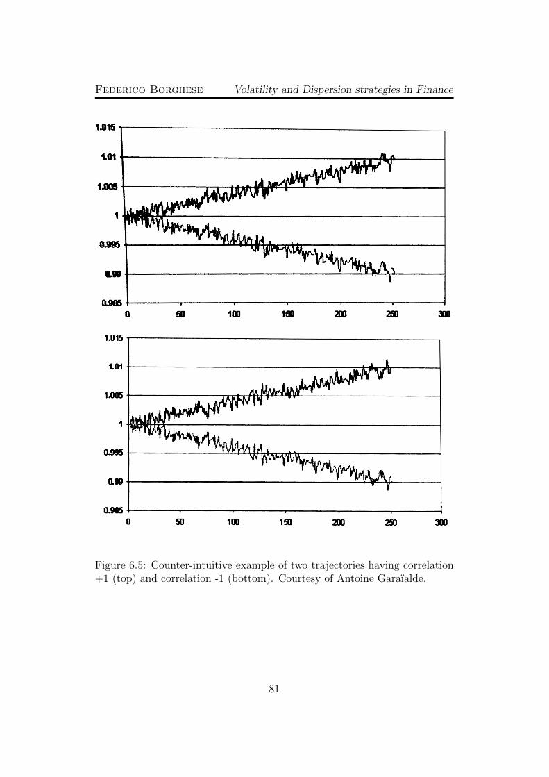
Federico Borghese Volatility and Dispersion strategies in Finance
Figure 6.5: Counter-intuitive example of two trajectories having correlation+1 (top) and correlation -1 (bottom). Courtesy of Antoine Garaıalde.
81

Acknowledgements
Before anyone else, I would like to thank my Thesis Supervisor MaurizioPratelli. Throughout the years, he has taught me a lot about mathematicalfinance and provided invaluable advice. He has been very kind and helpful,especially because of the unusual situation where we collaborated by emails,and I appreciate the time he spent writing me and helping me with the formsand documents.
Heartfelt thanks also to my colleagues in J.P. Morgan. First of all, my GuruAntoine Garaıalde: every day he teaches me something new. He involved mein thrilling projects about various Volatility and Correlation trades, gave meadvice and stimulated my curiosity. All of that with a good amount of goodmood and laughter.I want to thank Arnaud Jobert, for the trust he gave me since the beginning,for the way he makes me feel welcome and for the amazing opportunity tojoin his team.Thanks to Guillaume Flamarion, who shares with me his impressive experi-ence and knowledge of the job and helps me gain visibility within the firm.Thanks also to Andrea Santacroce, who is the main reason why I am in thisamazing Structuring team in J.P. Morgan. From the moment we met inParis, he opened my eyes on my career ambitions and gave me invaluableadvice. And since the start of my position in J.P. Morgan, he dedicated hugeamounts of his time to help me, teach me, guide me.Thanks to Johannes Ingerfurth for teaching and helping me as a friend does.Many thanks to all the rest of the Structuring and Trading team, especiallyto Julien Nizard, for their help and guidance and for making me happy everyday to go to work.
82

Federico Borghese Volatility and Dispersion strategies in Finance
Thanks to my mum, for her fond love and support and for making mealways feel special. Despite the distance, she is always ready to pick up thephone and make us feel close.Thanks to my dad for his high consideration towards me, for his love and forvisiting me in London.Thanks to my brother, for not visiting me in London :) and for always mak-ing me laugh and feel like a kid.
Heartfelt thanks to Cristofer. Literally, without him I would have nevergraduated. He did so much for me. He came to London many times andkept me smiling in the hardest situations. He supported me every day at thephone. He would do anything to help me, and he did help me so much indeed.
Thanks to all my friends, for always keeping in touch despite the distance,for their love and support.Thanks to my friends from Rome, for their long-lasting friendship: Patonza,Dark Lady, Bionda, Lumiere, Piccola Panda, Foca, Cagna, Piva.Thanks to my friends in Pisa, who made my four years in Tuscany re-ally amazing: Gatta, Vicky, Pamela, Alessia, Erika, Marsha&Labrador, Ila,Orsetto&Enrico, Terranova, Lemurino&Cigno, Megumi&Psycho, Davide,Chiaretta, Ghionce, le Gallinelle (Serena, Angelica, Francesca, Chiara, Giu-lia), Marti, Giulia la Rossa, Luca, Marco, Micky, Anto, Elena&Lori, il Principe,Dani and everybody else (there would be no space here to list you all!).Thanks to my flatmate Mathieu for always keeping me in good mood andthanks to Silvia for great nights in London and her new promising friendship!!
83
Bibliography
[1] D. Revuz, M. Yor, Continuous Martingales and Brownian Motion, 1991
[2] T. Bjork, Arbitrage Theory in Continuous Time, 2004
[3] J. Hull, Options, Futures and Other Derivatives, 2009 (Seventh Edition)
[4] R. Lee, Weighted Variance Swap, 2009
[5] K. Demeterfi, E. Derman, M. Kamal, J. Zou, More Than You EverWanted To Know About Volatility Swaps, Goldman Sachs QuantitativeResearch, 1999
84