MPRAMunich Personal RePEc Archive

Kuhn-Tucker theorem foundations andits application in mathematicaleconomics

Dushko Josheski and Elena Gelova

University Goce Delcev-Stip

12. October 2013

Online at http://mpra.ub.uni-muenchen.de/50598/MPRA Paper No. 50598, posted 14. October 2013 09:11 UTC

1

KUHN-TUCKER THEOREM FOUNDATIONS AND ITS APPLICATION IN THE

MATHEMATICAL ECONOMICS

Dushko Josheski Elena Gelova

dusko.josevski@ugd.edu.mk ; elena.gelova@ugd.edu.mk

University Goce Delcev-Stip,R.Macedonia

Abstract

In this paper the issue of mathematical programming and optimization has being

revisited. The theory of optimization deals with the development of models and methods

that determine optimal solutions to mathematical problems defined. Mathematical model

must be some function of any solution that accompanies a value which is a measure of

quality. In mathematics Kuhn-Tucker conditions are first order necessary conditions for

a solution in non-linear programming. Under, certain specific circumstances, Kuhn-

Tucker conditions are necessary and sufficient conditions as well. In this paper it is also

introduced the use of these mathematical methods of optimization in economics.

Keywords: Kuhn-Tucker conditions, nonlinear optimization, mathematical economics

2

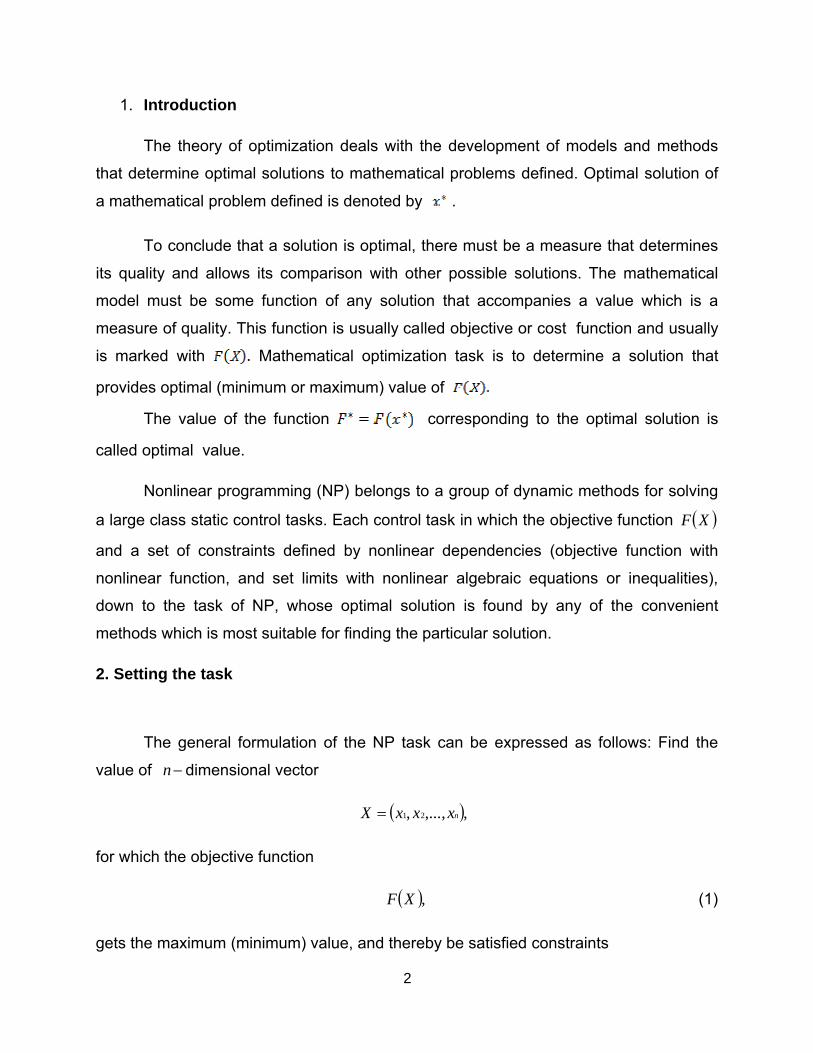
1. Introduction

The theory of optimization deals with the development of models and methods

that determine optimal solutions to mathematical problems defined. Optimal solution of

a mathematical problem defined is denoted by .

To conclude that a solution is optimal, there must be a measure that determines

its quality and allows its comparison with other possible solutions. The mathematical

model must be some function of any solution that accompanies a value which is a

measure of quality. This function is usually called objective or cost function and usually

is marked with Mathematical optimization task is to determine a solution that

provides optimal (minimum or maximum) value of

The value of the function corresponding to the optimal solution is

called optimal value.

Nonlinear programming (NP) belongs to a group of dynamic methods for solving

a large class static control tasks. Each control task in which the objective function XF

and a set of constraints defined by nonlinear dependencies (objective function with

nonlinear function, and set limits with nonlinear algebraic equations or inequalities),

down to the task of NP, whose optimal solution is found by any of the convenient

methods which is most suitable for finding the particular solution.

2. Setting the task

The general formulation of the NP task can be expressed as follows: Find the

value of n dimensional vector

,,...,, 21 nxxxX

for which the objective function

,XF (1)

gets the maximum (minimum) value, and thereby be satisfied constraints

3

,0XG (2)

,0X

where XG is m dimensional vector function whose components are

.,...,, 21 XgXgXg m

The mathematical model of the general task of NP (1) - (2), which is written in the

most general form, involves determining those values nxxx ,...,, 21 for which the objective

function

,,...,, 21 nxxxF

gets the maximum (minimum) value when the constraints

,0,...,, 21 ni xxxg ,,...,2,1 mi

,0jx .,...,2,1 nj

Often, it is common expressions in equations (2) are called conditions and restrictions

inequality. Indexes m and n mutually independent, i.e. m can be less, equal or greater

than n . Functions XF and ,Xgi ,,...,2,1 mi in general are nonlinear functions,

hence the name nonlinear programming.

For convex functions the task of NP formulated in the form (1) - (2), which requires a

minimum of objective function XF . However, concave objective function and a set of

constraints, the task of NP is formulated through the maximization of the objective

function XF set limits 0Xgi , .,...,2,1 mi Reducing task of (1) - (2) the task of

maximizing the objective function

XF , (1’)

the set of constraints

,0X (2’)

4

and bring the task (1 ') - (2') to the task of (1) - (2), it is not difficult, given that in the

first and in the second case it is necessary to alter the sign function, i.e. instead XF

you need to put XF , or instead XG put XG and change the sign in the

inequality of set constraints. In the opposite case requests are handled in the same

way.

Therefore, no matter whether we are talking about the task (1) - (2) or task (1 ') -

(2'). This feature will often use, and when it will have in mind that when it comes to the

task (1) - (2), while talking about the task (1 ') - (2'), and vice versa. Because of these

two tasks, which are formally different, is referred to as a single task.

3. Theorem of Kuhn and Tucker

Theorem of Kuhn and Tucker1 in the literature often referred to as theorem

saddle point. Occupies a central place in the theory of convex programming and is a

generalization of the classical method of Lagrangian multipliers.

As is known, the method of Lagrangian multiples (multipliers) provides finding

extreme values of functions which depend on several variables, and constraints that are

set by default draws. However, the theorem of Kuhn and Tucker generalizes method of

Lagrangian multipliers, expanding it by finding the extreme values of a function that

depends on several variables, but when set limits are not given but only draws and

inequality. Theorem of Kuhn and Tucker gives a necessary and sufficient condition must

meet the vector *XX , which is the solution of the task ( 1 ) - ( 2 ) . The criteria for

meeting the necessary and sufficient condition is established and verified based on

1 Kuhn H.Tucker A., Non-Linear Programming, Proceedings of the Second Berkeley

Symposium on Mathematical Statistics and Probality, University of California Press,

Berkeley, California, 1950

5

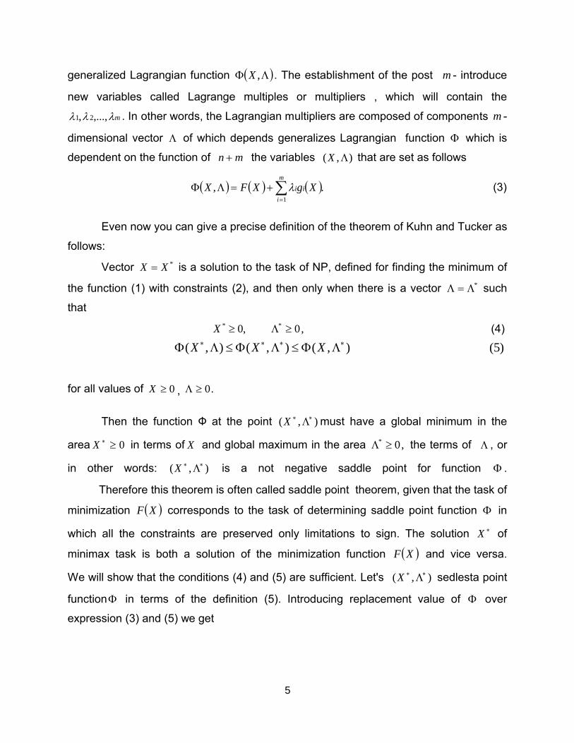
generalized Lagrangian function ,X . The establishment of the post m - introduce

new variables called Lagrange multiples or multipliers , which will contain the

m ,...,, 21 . In other words, the Lagrangian multipliers are composed of components m -

dimensional vector of which depends generalizes Lagrangian function which is

dependent on the function of mn the variables ),( X that are set as follows

.,1

m

i

XgXFX ii (3)

Even now you can give a precise definition of the theorem of Kuhn and Tucker as

follows:

Vector *XX is a solution to the task of NP, defined for finding the minimum of

the function (1) with constraints (2), and then only when there is a vector * such

that

,0* X ,0* (4)

for all values of 0X , .0

Then the function Ф at the point ),( X must have a global minimum in the

area 0X in terms of X and global maximum in the area ,0* the terms of , or

in other words: ),( X is a not negative saddle point for function .

Therefore this theorem is often called saddle point theorem, given that the task of

minimization XF corresponds to the task of determining saddle point function in

which all the constraints are preserved only limitations to sign. The solution X of

minimax task is both a solution of the minimization function XF and vice versa.

We will show that the conditions (4) and (5) are sufficient. Let's ),( X sedlesta point

function in terms of the definition (5). Introducing replacement value of over

expression (3) and (5) we get

( , ) ( , ) ( , ) (5)X X X

6

,11

**

1

** **

m

i

m

i

m

i

XgXFXgXFXgXF iiiiii

for all values of

,0X .0

As the left inequality in the previous expression must be met for each , then

,0* Xgi ,,...,2,1 mi

i.e. X an admissible plan, because the area belongs to (D) which is defined by a set

of constraints and conditions

.01

**

m

i

Xgii

The right inequality thus taking shape

,1

* *

m

i

XgXFXF ii

for all values ,0X where given the condition ,0* it follows that

*XF XF ,

for all values 0X that satisfy the conditions

,0Xgi ,,...,2,1 mi

because the value of X is the solution of the task (1) - (2).

That the conditions (4) and (5) are required to obtain the regularity assumption upon

which, in a pinch, there is at least one point X X (admissible plan) such that

Xig <0, ,,...,2,1 mi

it is necessary to emphasize that the introduction of the presumption of regularity is

unnecessary for all functions Xgi which appear as linear features (details of the proof

7

here will not say). In any case, when the set limits is linear theorem of Kuhn and Tucker

does not have any restrictions.

When functions XF and Xgi are differential, conditions (4) and (5) are

equivalent to the following 'local' conditions of Kuhn - Tucker:

,0

,0

,0

*

*

**,

**,

j

jj

j

x

xx

x

X

X

,,...,2,1 nj (6)

.0

,0

,0

*

**,

**,

i

ii

i

X

X

,,...,2,1 mi (7)

The terms of the Kuhn - Tucker remain valid and in some changes to the setup

of the task (1) - (2). Thus, for example, you happen to setting task constraints not

present ,0jx .,...,2,1 nj In this case the three conditions (6) are replaced with only

one condition

.0

**,

Xjx (8)

For the case when the functions Xgi are linear, the conditions (7) is replaced by the

condition

,0**,

Xi (9)

which is a second way of writing requirement

,0Xgi .,...,2,1 mi

8

Multipliers i , mi ,...,2,1 here are not restricted in terms of sign.

Finally, when the constraints Xgi are linear and defined by the equation

,0Xgi

conditions (6) and (7) are reduced to conditions (8) and (9), which represent a classic

case of the method of Lagrange multipliers.

4.Constrained and unconstrained optimization

In the classical optimization problem, the first condition for optimization is the first partial

derivative of the Lagrangian function. Now, in nonlinear programming2there also exists

a similar type of first-order condition, Chiang, Wainwright (2005)3. First will take one

variable case and then two variables case. So let’s consider this problem:

(10)

subject to (11)

In the previous expression it is assumed that is differentiable. Chiang

,Wainwright(2005),here pose three solutions, first ,and this is an interior

solution of the problem4. Second, also there may be solution where ,and

.An the third solution is . And these three conditions can be

consolidated into one single condition:

(12)

2Kuhn,H.,W.,,Tucker,W.,A.,(1951), Nonlinear programming, Second Berkeley symposium on Mathematical statistics and probability3 Chiang, A., Wainwright, K.,(2005), Fundamental methods of mathematical economics, 4thed.,Mcgraw Hill 4 This solution is interior because it lies is the region below the curve, where the feasible region is.

9

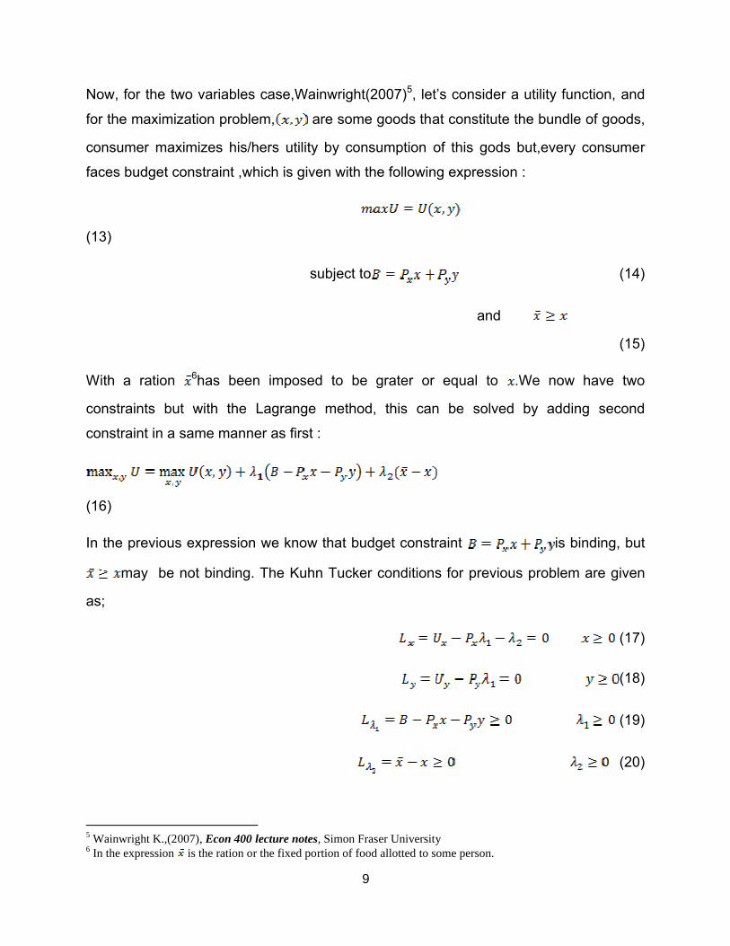
Now, for the two variables case,Wainwright(2007)5, let’s consider a utility function, and

for the maximization problem, are some goods that constitute the bundle of goods,

consumer maximizes his/hers utility by consumption of this gods but,every consumer

faces budget constraint ,which is given with the following expression :

(13)

subject to (14)

and

(15)

With a ration 6has been imposed to be grater or equal to .We now have two

constraints but with the Lagrange method, this can be solved by adding second

constraint in a same manner as first :

(16)

In the previous expression we know that budget constraint is binding, but

may be not binding. The Kuhn Tucker conditions for previous problem are given

as;

(17)

(18)

(19)

(20)

5 Wainwright K.,(2007), Econ 400 lecture notes, Simon Fraser University6 In the expression is the ration or the fixed portion of food allotted to some person.

10

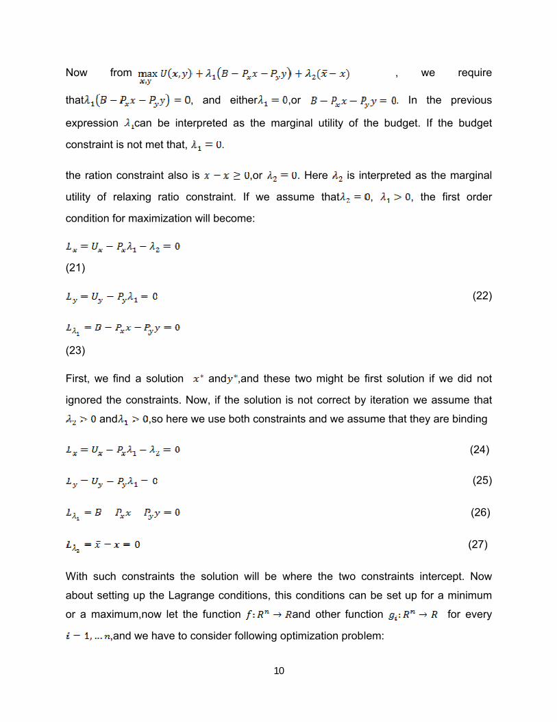
Now from , we require

that , and either ,or . In the previous

expression can be interpreted as the marginal utility of the budget. If the budget

constraint is not met that, .

the ration constraint also is ,or . Here is interpreted as the marginal

utility of relaxing ratio constraint. If we assume that , , the first order

condition for maximization will become:

(21)

(22)

(23)

First, we find a solution and ,and these two might be first solution if we did not

ignored the constraints. Now, if the solution is not correct by iteration we assume that

and ,so here we use both constraints and we assume that they are binding

(24)

(25)

(26)

(27)

With such constraints the solution will be where the two constraints intercept. Now

about setting up the Lagrange conditions, this conditions can be set up for a minimum

or a maximum,now let the function and other function for every

,and we have to consider following optimization problem:

11

(28)

Subject to (29)

The set of points , is a feasible set. It means that is every point

x lies in that area the solution is optimal. Now if there exist such a solution that

where ,now we say that ith constraint is a binding constraint, Varian (1992)7.

Otherwise if ,we say that ith constraint is a slack constraint or that is not

binding. Now, the Kuhn-Tucker theorem states as in Varian (1992), that, if there such a

point that solves the optimization problem subject to ,

and the constraint qualification holds at , then there exist a set of Kuhn-Tucker

multipliers , such that this equality holds

i.e. ,furthermore this conditions for slackness hold such that

, 8and the second condition . Comparing the Kuhn-

Tucker theorem to the Lagrange multiplier theorem the major difference is that the signs

of the Kuhn-Tucker multipliers can be positive, and the Lagrange multipliers signs can

be positive or negative. The Lagrangian for this problem subject to

, is given as, , so when the problem is set

to be like this Kuhn-Tucker conditions will always be non-negative9.Now, the envelope

theorem10, exist in its regular version (unconstrained), and irregular version constrained,

this is basic theorem for solving problems in microeconomics. Now lets consider some

arbitrary problem11:

(30)

Where the function, where gives the maximized value of the objective function

as a function of parameter . Now let be the argument of the maximum value of ,

7 Varian, R.,H.,(1992),Microeconomic analysis, third edition 8 is some whole real number 9 That is because , and the sum of negative numbers is negative number 10Kimball, W. S., Calculus of Variations by Parallel Displacement.London: Butterworth, p. 292, 1952.11E3m-lab,Lecture notes,(2011),Basics for mathematical economics,National technical university of Athens, Institute of communications and computer systems

12

that solves the maximization problem in terms of the parameter . Now, that

(31)

That is derivative of M with respect to a is given by the partial derivative of with

respect to .

5. Conclusion

In mathematics Kuhn-Tucker conditions are first order necessary conditions for a

solution in non-linear programming. Under, certain specific circumstances, Kuhn-Tucker

conditions are necessary and sufficient conditions as well. Mathematical programming

is capable of handling inequality constraints, and apart from its obvious application to

industrial problems and in business management, it also enables economists to see the

theory of consumption, production, and resource allocation in a new light, Chiang

(1984).But some of the limitations of mathematical programming are: variables are

assumed to be continuous (in practice more of the variables may admit integer

values),and the static nature of the solution.

13

References

1. Kuhn H.Tucker(1950). A, Non-Linear Programming, Proceedings of the

Second Berkeley Symposium on Mathematical Statistics and Probality,

University of California Press, Berkeley, California, 1950

2. Chiang, A., Wainwright, K.,(2005), Fundamental methods of mathematical

economics, 4thed.,Mcgraw Hill

3. Wainwright K.,(2007), Econ 400 lecture notes, Simon Fraser University

4. Varian, R.,H.,(1992),Microeconomic analysis, third edition

5. Kimball, W. S., Calculus of Variations by Parallel Displacement.London:

Butterworth, p. 292, 1952.

6. E3m-lab,Lecture notes,(2011),Basics for mathematical economics,National

technical university of Athens, Institute of communications and computer

systems