MPRAMunich Personal RePEc Archive

Applying CHAID for logistic regressiondiagnostics and classification accuracyimprovement

Evgeny Antipov and Elena Pokryshevskaya

The State University Higher School of Economics

2009

Online at https://mpra.ub.uni-muenchen.de/21499/MPRA Paper No. 21499, posted 29. March 2010 07:30 UTC

1

Evgeny Antipov

Affiliation: The State University Higher School of Economics and The Center for Business

Analysis

E-mail address: eugene.antipov@gmail.com

Elena Pokryshevskaya

Affiliation: The State University Higher School of Economics and The Center for Business

Analysis

Country: Russia

E-mail address: e.pokryshevskaya@gmail.com

Applying CHAID for logistic regression diagnostics and classification

accuracy improvement

Abstract

In this study a CHAID-based approach to detecting classification accuracy heterogeneity across

segments of observations is proposed. This helps to solve some important problems, facing a

model-builder:

1. How to automatically detect segments in which the model significantly underperforms?

2. How to incorporate the knowledge about classification accuracy heterogeneity across

segments to partition observations in order to achieve better predictive accuracy?

The approach was applied to churn data from the UCI Repository of Machine Learning

Databases. By splitting the dataset into 4 parts, which are based on the decision tree, and

building a separate logistic regression scoring model for each segment we increased the accuracy

by more than 7 percentage points on the test sample. Significant increase in recall and precision

was also observed. It was shown that different segments may have absolutely different churn

2

predictors. Therefore such a partitioning gives a better insight into factors influencing customer

behavior.

Keywords: CHAID, logistic regression, churn prediction, performance improvement,

segmentwise prediction, decision tree

1 Introduction

Classification problems are very common in business and include credit scoring, direct

marketing optimization and customer churn prediction among others. Researchers develop and

apply more and more complex techniques to maximize the prediction accuracy of their models.

However, a common modeling problem is the presence of heterogeneity of classification

accuracy across segments. Therefore building one model for all observations and considering

only aggregate predictive accuracy measures may be misleading if a classifier performance

varies significantly across different segments of observations. To cope with such an undesirable

feature of classification models, analysts sometimes try to split the sample into several

homogeneous groups and build a separate model for each segment or employ dummy variables.

As far as we know, methods of automatic data partitioning in order to reduce such heterogeneity

have not received much attention in papers on classification problems: researchers usually use

some a priori considerations and make mainly univariate splits (e. g. by gender). Deodhar and

Ghosh (2007)1 stated that researchers most often do partitioning a priori based on domain

knowledge or a separate segmentation routine.

Some researchers have proposed CHAID as an aid for better specifying and interpreting a logit

model (Magidson, 19822, Ratner, 1997

3). In this paper the CHAID-based approach is used for

finding whether subgroups with significantly lower or higher than average levels of prediction

accuracy can be found in data after applying the binary logistic regression. This approach is

3

employed for diagnostic purposes as well as for improving the initial model. We demonstrate

that the proposed method can be used for splitting the dataset into several segments, followed by

building separate models for each segment, which leads to a significant increase in classification

accuracy both on training and test datasets and therefore, enhances logistic regression.

2 Models employed in the study

Logistic regression

In the logit (logistic) regression model, the predicted values for the dependent variable will

always be greater than (or equal to) 0, or less than (or equal to) 1. This is accomplished by

applying the following regression equation4:

0 1 1 n n

0 1 1 n n

b b x b x

b b x b x

ey

1 e

The name logit stems from the fact that one can easily linearize this model via the logit

transformation. Suppose we think of the binary dependent variable y in terms of an underlying

continuous probability p, ranging from 0 to 1. We can then transform that probability p as:

e

pp' log

1 p

This transformation is referred to as the logit or logistic transformation. Note that p' can

theoretically assume any value between minus and plus infinity. Since the logit transform solves

the issue of the 0/1 boundaries for the original dependent variable (probability), we could use

those (logit transformed) values in an ordinary linear regression equation. In fact, if we perform

the logit transform on both sides of the logit regression equation stated earlier, we obtain the

standard linear regression model:

0 1 1 2 2 n np' b b x b x b x

For a comprehensive but accessible discussion of logistic regression we suggest reading Hosmer

et al. (20005) and Kleinbaum (1994

6).

4

Logistic regression is very appealing for several reasons: (1) logit modeling is well known, and

conceptually simple; (2) the ease of interpretation of logit is an important advantage over other

methods (e.g. neural networks); (3) logit modeling has been shown to provide good and robust

results in comparison studies7. As for database marketing applications, it has been shown by

several authors8 that logit modeling may outperform more sophisticated methods. Perhaps, the

most serious problem with logistic regression, failure to incorporate nonmonotonic relationships,

can be partly solved by numeric variables quantization (using classification trees, for example).

CHAID

CHAID is a type of decision tree technique, based upon adjusted significance testing (Bonferroni

testing). The acronym CHAID stands for Chi-squared Automatic Interaction Detector. It is one

of the oldest tree classification methods originally proposed by Kass (19809; according to Ripley,

199610

, the CHAID algorithm is a descendent of THAID developed by Morgan and Messenger,

197311

). CHAID will "build" non-binary trees (i.e., trees where more than two branches can

attach to a single root or node), based on a relatively simple algorithm that is particularly well

suited for the analysis of larger datasets. Also, because the CHAID algorithm will often

effectively yield many multi-way frequency tables (e.g., when classifying a categorical response

variable with many categories, based on categorical predictors with many classes), it has been

particularly popular in marketing research, in the context of market segmentation studies.4

CHAID output is visual and easy to interpret. Because it uses multiway splits, it needs rather

large sample sizes to work effectively as with small sample sizes the respondent groups can

quickly become too small for reliable analysis. In this study we use CHAID as a diagnostic

technique, which can be helpful in partitioning the dataset into several segments, which differ by

the misclassification error of logistic regression model.

5

CART

CART algorithm was introduced in Breiman et al. (198612

). A CART tree is a binary decision

tree that is constructed by splitting a node into two child nodes repeatedly, beginning with the

root node that contains the whole learning sample. The CART growing method attempts to

maximize within-node homogeneity. The extent to which a node does not represent a

homogenous subset of cases is an indication of impurity. For example, a terminal node in which

all cases have the same value for the dependent variable is a homogenous node that requires no

further splitting because it is "pure." For categorical (nominal, ordinal) dependent variables the

common measure of impurity is Gini, which is based on squared probabilities of membership for

each category. Splits are found that maximize the homogeneity of child nodes with respect to the

value of the dependent variable.

3 Methodology

CHAID-based diagnostics and classification accuracy improvement

Binary classifiers, such as logistic regression, use a set of explanatory variables in order to

predict the class to which every observation belongs. Let X1, …, Xn be the explanatory variables

included into the classification model; Yi - the observed class to which observation i belongs,

iY – the predicted class for this observation. Then variable Ci indicates whether the observation i

is misclassified (Ci=0) or not (Ci=1).

1. On the training sample build the decision tree, using the CHAID algorithm with Сi as a

dependent variable and with X1, …, Xn as the explanatory variables. Choose the

significance level you think is appropriate (in this study we will always use 5%

significance level). Nodes of the tree represent the segments which differ by the correct

classification rate. If no splits are made then classification accuracy is most likely to be

homogenous across segments of observations.

6

2. If the revealed segments significantly differ in classification accuracy rate (both from the

statistical and practical point of view) split the dataset into several non-overlapping

subsets according to the information you have from the above mentioned decision tree.

The number of segments primarily depends on the number of observations in different

nodes of the tree.

Although CHAID has been chosen, there are hardly any arguments against the idea of trying

other decision trees algorithms and choosing the best segmentation (from the point of view of an

analyst). The attractive features of the proposed approach are its simplicity and interpretability. It

can be easily implemented using widespread statistical packages such as PASW Statistics,

Statistica or SAS. Due to its data mining nature this method works best on rather large datasets

(over 1000 observations). However, as a purely diagnostic approach it may be applied to smaller

ones as well.

Data

To illustrate the introduced approach we use the churn dataset from the UCI Repository of

Machine Learning Databases13

. The case study associated with this dataset is as follows. The

early detection of potential churners enables companies to target these customers using specific

retention actions, and should subsequently increase profits. A telecommunication company

wants to determine whether a customer will churn or not in the next period, given billing data.

The dependent variable is whether the client churned or not. The explanatory variables are listed

in Table 1. As we use this dataset mainly to illustrate a rather general approach, we do not set

any specific misclassification costs or prior probabilities.

7

Table 1. Explanatory variables

Variable Name Variable Description Variable type

AccountLength Account Length (months) integer

IntlPlan International plan Dichotomous

VMailPlan Voice mail plan Dichotomous

VMail Message Number of voice mail messages integer

Day Mins Total day minutes continuous

Eve Mins Total evening minutes continuous

Night Mins Total night minutes continuous

Intl Mins Total international minutes continuous

CustServ Calls Number of calls to customer service integer

Before building the initial logit model we randomly divide our sample into training (2000 cases)

and test (1333 cases) sets.

Logistic regression modeling and diagnostics

The parameter estimates of Model 1 are presented in Table 2. We use backward stepwise

variable selection method with entry probability equal to 0.05 and removal probability equal to

0.1.

Table 2. Parameter Estimates of Model 1

Variable B Wald Sig. Exp(B)

Intercept -8,347 115,246 0,000

VMailPlan 1,990 11,921 0,001 7,318

IntlPlan -2,020 195,416 0,000 0,133

VMailMessage 0,035 3,663 0,056 1,035

8

DayMins 0,013 142,833 0,000 1,013

EveMins 0,007 39,328 0,000 1,007

NightMins 0,004 11,005 0,001 1,004

IntlMins 0,085 17,269 0,000 1,088

CustServCalls 0,511 170,799 0,000 1,666

Then we generate variable C (the indicator of correct classification). After that we build a

diagnostic CHAID decision tree (Fig. 1) using PASW Statistics 18 (SPSS Inc.), taking C as the

dependent variable and all the predictors listed in Table 1 as the explanatory variables. To obtain

segments large enough for the subsequent analysis we have set the minimum size of nodes to

200 observations.

9

Fig. 1. CHAID decision tree: accuracy of Model 1 (training sample)

From the diagnostic decision tree it is obvious that there is a significant difference between the

accuracy in 4 groups automatically formed on the basis of total day minutes and international

plan variables. The first segment has the lowest percentage of correctly classified customers

(64.2%) and consists of those who have chosen the international plan, the other three segments

include those who do not use the international plan: these segments are based on the number of

total day minutes. The highest classification accuracy is within the segment of customers who

use 180.6 – 226.1 total day minutes (95.8%).

10

We quantify the heterogeneity of classification accuracy using the following normalized measure

of dispersion:

2

1

10.125

N

i i

i

N

i

i

PCC PCC n

n

CVPCC

Here iPCC stands for the percentage correctly classified in segment i, PCC is the percentage

correctly classified in the whole training sample, in is the size of each segment, N is the number

of segments.

Some possible ways of improving the model are listed below:

1. Override the model in the least predictable segments.

2. Split the dataset and build a separate model for each of the revealed segments.

3. Use some sort of ensembling with weights proportional to the probability that the classifier

works best for this segment.

Although the third approach may be rather promising, its development requires some further

research. We use the second alternative and build separate models for 4 large segments of data,

revealed with the help of the CHAID decision tree (we set minimum node size to 300 to make

our results robust by operating with rather large segments). The parameter estimates for Model 2

(the logistic regressions built on three segments separately) are presented in Table 3.

11

Table 3. Parameter Estimates of Model 2

Segment Variable B Wald Sig. Exp(B)

International Plan

Intercept -5,113 36,162 0,000

EveMins 0,004 3,090 0,079 1,004

IntlMins 0,343 37,477 0,000 1,410

CustServCalls 0,167 3,092 0,079 1,182

No International plan,

Total day minutes<=180.6

Intercept -4,272 71,615 0,000

EveMins -0,005 4,172 0,041 0,995

CustServCalls 1,174 199,041 0,000 3,235

No International plan,

180.6<=Total day minutes<=226.1

Intercept -13,115 19,664 0,000

EveMins 0,006 3,242 0,072 1,006

CustServCalls 0,271 5,128 0,024 1,312

AccountLength 0,010 5,687 0,017 1,010

VMailPlan -3,197 4,633 0,031 0,041

VMailMessage 0,099 5,482 0,019 1,104

DayMins 0,029 4,785 0,029 1,029

NightMins 0,007 3,750 0,053 1,007

No International plan,

Total day minutes>=226.1

Intercept -44,114 94,019 0,000

EveMins 0,052 84,346 0,000 1,053

IntlMins 0,165 8,164 0,004 1,180

VMailPlan -15,162 14,828 0,000 0,000

VMailMessage 0,237 4,790 0,029 1,267

DayMins 0,101 77,305 0,000 1,106

NightMins 0,027 42,572 0,000 1,027

The reference category is: Did not churn

12

From Table 3 it is obvious that the sets of automatically selected predictors are different for each

of the four segments, which means the idea of building separate models for each segment is most

likely to be a reasonable one. Not only this can lead to increased accuracy, but also can give

managers some ideas on how to increase loyalty. For example, customers with more than 226.1

total day minutes may be extremely unsatisfied with the voice mail plan they are offered. The

most appropriate interpretation may be provided only by an expert from the telecommunication

company, who will probably find plenty of insights in such regression analysis output.

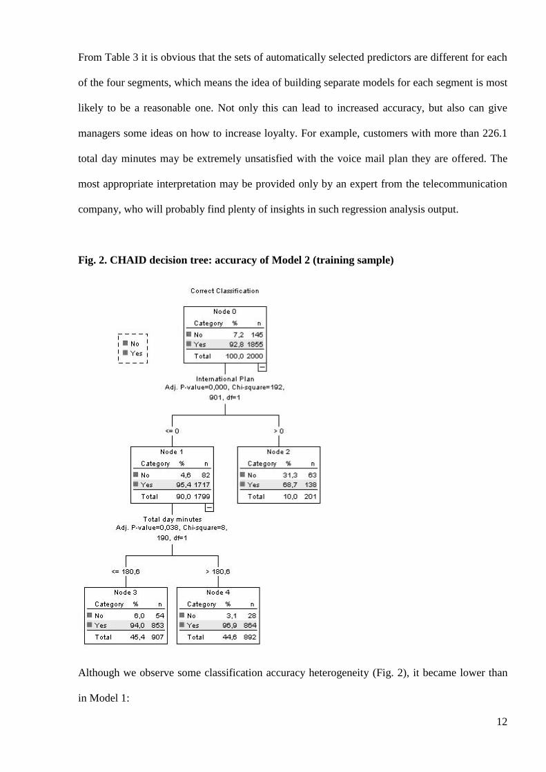
Fig. 2. CHAID decision tree: accuracy of Model 2 (training sample)

Although we observe some classification accuracy heterogeneity (Fig. 2), it became lower than

in Model 1:

13

2

1

10.088

N

i i

i

N

i

i

PCC PCC n

n

CVPCC

Another important improvement is the increase in Percentage Correctly Classified which reached

92.8% for the training sample and 92.1% for the test simple, compared to 87% and 85%

correspondingly for Model 1 (see Tables 4 and 5).

Table 4. Classification table for Model 1

Training sample Test sample

Predicted Category Predicted Category

Did not churn Churned Did not churn Churned

Observed

category

Did not churn 1681 36 1101 32

Churned 223 60 168 32

Table 5. Classification table for Model 2

Training sample Test sample

Predicted Category Predicted Category

Did not churn Churned Did not churn Churned

Observed

category

Did not churn 1687 30 1108 25

Churned 115 168 80 120

When dealing with class imbalance it is often useful to look at recall and precision measures:

TPRecall

TP FN

,

TPPrecision

TP FP

, where TP is the number of true positive, FN – the

number of false negative and FP is the number of false positive predictions. Recall (true positive

rate) has increased (from 16% on test sample for Model 1 up to 60% for Model 2), as well as

14

precision (from 50% on test sample for Model 1 up to 82.8% for Model 2). This means that

Model 2 allows targeting a larger share of potential churners than Model 1 and that a greater

percent of customers indicated by the model as potential churners are worth targeting. From

economic point of view the loyalty program based on Model 2 is most likely to be more efficient

than the one based on Model 1.

Logistic Regression vs. CHAID and CART

To show that Model 2 is based on a competitive modeling approach, we have compared test

sample AUC (Area under the ROC Curve) for Model 2, Model 1 and two data mining

classification techniques: CHAID and CART. To avoid overfitting, the minimum size of a

classification tree node was set at 100.

Table 6. Area under the curve comparison

Model AUC

Logistic Regression (Model 1) 0.812

Logistic Regression (Model 2) 0.890

CHAID 0.691

CART 0.835

Standard logistic regression performed worse than CART, but better than CHAID. Model 2 has

the highest AUC.

Although logistic regression tends to become an old-fashioned instrument, we believe it will still

complement new data mining methods in managerial applications due to the following reasons:

1. Unlike classification trees, it gives a continuous predicted probability, which is helpful when

direct marketers have to sort prospects by their propensity to churn, buy, etc. and do not want to

15

obtain too many tied ranks (even an ensemble of 2-3 decision trees may sometimes lead to

insufficient number of different predicted probabilities).

2. It may be preferred by experienced analyst who are not satisfied with automatic model-

building procedures and want to develop a tailor-made model with interactions and test some

particular hypotheses.

3. It generally requires smaller samples than classification trees.

4. It often performs better than some state of the art techniques in terms of AUC, accuracy and

other performance measures.

5. The standard logistic regression can be enhanced using bagging or approaches like the one

described in this paper, leading to at least as high performance as of well-established machine

learning algorithms.

6. Logistic regression failure to incorporate nonmonotonic relationships can be partly solved by

numeric variables quantization (using classification trees, for example).

4 Conclusions and future work

In some applications, due to the heterogeneity of the data it is advantageous to learn

segmentwise prediction models rather than a global model. In this study we have proposed a

CHAID-based approach to detecting classification accuracy heterogeneity across segments of

observations. This helps to solve 2 important problems, facing a model-builder:

1. How to automatically detect and visualize segments in which the model significantly

underperforms?

2. How to incorporate the knowledge about classification accuracy heterogeneity across

segments of observations to split cases into several segments in order to achieve better predictive

accuracy?

16

We applied our approach to churn data from the UCI Repository of Machine Learning

Databases. By splitting the dataset into 4 parts, which are based on the decision tree, and

building a separate logistic regression scoring model for each segment we increased the accuracy

by more than 7 percentage points on the test sample. From economic point of view the loyalty

program based on Model 2 is most likely to be much more efficient than the one based on Model

1 thanks to an increase in recall (from 16% to 60%) and precision (from 50% to 82.8%). We

have revealed that different segments may have absolutely different churn predictors. Therefore

such a partitioning may give both prediction accuracy improvement and a better insight into

factors influencing customer behavior. By calculating the AUC it was shown that Model 2 has

outperformed CHAID and CART.

In our further research we plan to study, whether better performance may be achieved by using

classification tree algorithms other than CHAID together with logistic regression. Applying

decision trees to improve other classifiers such as Support Vector Machines, Random Forests

etc. may also be a direction for future work.

References

1. Deodhar, M., Ghosh, J. (2007) A framework for simultaneous co-clustering and learning

from complex data. Proceedings of the 13th ACM SIGKDD international conference on

Knowledge discovery and data mining; 12-15 August 2007, San Jose, California, USA.

2. Magidson, J. (1982) Some Common Pitfalls in Causal Analysis of Categorical Data.

Journal of Marketing Research, Vol. 19, No. 4, Special Issue on Causal Modeling (Nov.,

1982), pp. 461-471.

3. Ratner, B. (2003) Statistical modeling and analysis for database marketing: effective

techniques for mining big data. Chapman & Hall/CRC.

17

4. Hill, T. and Lewicki, P. (2007) STATISTICS Methods and Applications. StatSoft, Tulsa,

OK.

5. Hosmer, David W.; Stanley Lemeshow (2000). Applied Logistic Regression, 2nd ed. New

York; Chichester, Wiley.

6. Kleinbaum, D. G. 1994. Logistic Regression: A Self-Learning Text. New York: Springer-

Verlag.

7. Neslin, S., Gupta, S., Kamakura, W., Lu, J. and Mason, C. (2006) Detection defection:

Measuring and understanding the predictive accuracy of customer churn models. Journal of

Marketing Research 43(2): 204–211.

8. Levin, N. and Zahavi, J. (1998) Continuous predictive modeling, a comparative analysis.

Journal of Interactive Marketing 12: 5–22.

9. Kass, G.V. (1980) An Exploratory Technique for Investigating Large Quantities of

Categorical Data. Journal of Applied Statistics 29(2): 119-127.

10. Ripley, B.D. (1996) Pattern recognition and neural networks. Cambridge: Cambridge

University Press.

11. Morgan, J.N. and Messenger, R.C. (1973) THAID: A sequential analysis program for the

analysis of nominal scale dependent variables. Institute of Social Research, University of

Michigan, Ann Arbor. Technical report.

12. Breiman, L., J. H. Friedman, R. A. Olshen, and C. J. Stone. (1984) Classification and

Regression Trees. New York: Chapman & Hall/CRC.

13. Blake, C. L. and Merz, C. J., Churn Data Set, UCI Repository of Machine

Learning Databases, http://www.sgi.com/tech/mlc/db/. University of

California, Department of Information and Computer Science, Irvine, CA,

1998.