MPRAMunich Personal RePEc Archive

An Empirical Investigation of theEmergence of Money: ContrastingTemporal Difference and OpportunityCost Reinforcement Learning

Germain Lefebvre and Aurelien Nioche and Sacha

Bourgeois-Gironde and Stefano Palminteri

2018

Online at https://mpra.ub.uni-muenchen.de/85586/MPRA Paper No. 85586, posted 29 March 2018 17:43 UTC

Classification: SOCIAL SCIENCE, Economic Sciences, Psychological and Cognitive Sciences Title: An Empirical Investigation of the Emergence of Money: Contrasting Temporal Difference and Opportunity Cost Reinforcement Learning (129/135 max) Short Title: An Empirical Investigation of Money’s Emergence (48/50 max) Germain Lefebvre1,2,3*, Aurélien Nioche, †Sacha Bourgeois-Gironde4,*, †Stefano Palminteri2,3,5,*

Authors Affiliations: 1Laboratoire d’économie Mathématique et de Microéconomie Appliquée, Université Panthéon-Assas, Paris, FR 2Laboratoire de Neurosciences Cognitives, Institut National de la Santé et de la Recherche Médicale, Paris, FR 3Département D'études Cognitives, Ecole Normale Supérieure, Paris, FR 4Institut Jean-Nicod, Ecole Normale Supérieure, Paris, FR 5Institut d'Etude de la Cognition, Université de Recherche Paris Sciences et Lettres, Paris, FR † Similar contributions; the senior authors are listed in alphabetical order. Corresponding Authors: Germain Lefebvre*, Stefano Palminteri* LNC Ecole Normale Supérieure Département d'Études Cognitives 29, rue d'Ulm 1st floor, right 75005 Paris, France germain.lefebvre@ens.fr, stefano.palminteri@ens.fr Sacha Bourgeois-Gironde* Institut Jean-Nicod UMR 8129 Pavillon Jardin Ecole Normale Supérieure 29, rue d'Ulm F-75005 Paris, France sbgironde@gmail.com

Keywords: Theoretical Search Model, Reinforcement Learning, Speculative Behavior, Temporal Difference Learning, Counterfactual Learning, Opportunity Costs

Abstract Money is a fundamental and ubiquitous institution in modern economies. However, the question of its emergence remains a central one for economists. The monetary search-theoretic approach studies the conditions under which commodity money emerges as a solution to override frictions inherent to inter-individual exchanges in a decentralized economy. Although among these conditions, agents' rationality is classically essential and a prerequisite to any theoretical monetary equilibrium, human subjects often fail to adopt optimal strategies in tasks implementing a search-theoretic paradigm when these strategies are speculative, i.e., involve the use of a costly medium of exchange to increase the probability of subsequent and successful trades. In the present work, we hypothesize that implementing such speculative behaviors relies on reinforcement learning instead of lifetime utility calculations, as supposed by classical economic theory. To test this hypothesis, we operationalized the Kiyotaki and Wright paradigm of money emergence in a multi-step exchange task and fitted behavioral data regarding human subjects performing this task with two reinforcement learning models. Each of them implements a distinct cognitive hypothesis regarding the weight of future or counterfactual rewards in current decisions. We found that both models outperformed theoretical predictions about subjects' behaviors regarding the implementation of speculative strategies and that the latter relies on the degree of the opportunity costs consideration in the learning process. Speculating about the marketability advantage of money thus seems to depend on mental simulations of counterfactual events that agents are performing in exchange situations.

Significance Statement In the present study, we applied reinforcement learning models that are not classically used in experimental economics to a multi-step exchange task of the emergence of money derived from a classic search-theoretic paradigm for the emergence of money. This method allowed us to highlight the importance of counterfactual feedback processing of opportunity costs in the learning process of speculative use of money and the predictive power of reinforcement learning models for multi-step economic tasks. Those results constitute a new step toward understanding the learning processes at work in multi-step economic decision making and the cognitive micro-foundations of the macro-economic use of money.

Introduction Money is both a very complex social phenomenon and easy to manipulate in everyday basic transactions. It is an institutional solution to common frictions in an exchange economy, such as the absence of double coincidence of wants between traders (1). It is of widespread use in spite of its being dominated in terms of rate of return by all other assets (2). However, it can be speculatively used in a fundamental sense: its economically dominated holding can be justified by the anticipation of future trading opportunities that are not available at the present moment but will necessitate this particular holding. In this study, we concentrate on a paradigm of commodity-money emergence in which one of the goods exchanged in the economy becomes the selected medium of exchange in spite of its storage being costlier than any other good. This is typical monetary speculation, in contrast to other types of speculation, which consist in expecting an increased price on the market of a good in the future. The price of money does not vary – only the opportunity that it can afford in the future does. This seems to us to be an important feature of speculative economic behavior relative to the otherwise apparently irrational holding of such a good. We study whether individuals endowed with some information about future exchange opportunities will tend to consider a financially dominated good as a medium for exchange.

Modern behaviorally founded theories of the emergence of money and monetary equilibrium (3, 4) are jointly based on the idea of minimizing a trading search process and on individual choices of accepting, declining, or postponing immediate exchanges at different costs incurred. We focus on an influent paradigm by Kiyotaki and Wright (KW hereafter) (4) in which the individual choice of accepting temporarily costly exchanges due to the anticipation of later better trading opportunities is precisely stylized as a speculative behavior and yields a corresponding monetary equilibrium. The environment of this paradigm consists of N agents specialized in terms of both consumption and production in such a manner that there is initially no double coincidence of wants. Frictions in the exchange process create a necessity for at least some of the agents to trade for goods that they do not produce or consume, which are then used as media of exchange. The ultimate goal of agents – that is, to consume – may then require multiple steps to be achieved. The most interesting part is that in some configurations, the optimal medium of exchange (i.e., the good that maximizes expected utility because of its relatively high marketability) can be concomitantly the costlier good to store. Accepting this costly medium of exchange refers in the KW paradigm to the "speculative strategy": the agent accepts carrying the high storing cost burden to maximize its chance to consume in the future. Our question is how individuals can learn to use this multi-step speculative strategy in this environment, disregarding current cost increases in favor of longer-term benefits. It therefore locates at the intersection of a particular type of economic game, an application of learning models to individual behaviors in this type of game, and an underlying question about the cognitive underpinnings of the speculative use of money.

In the last few decades, behavioral economics experiments have repeatedly suggested that basic cognitive processes such as reinforcement learning potentially better accounts for subjects’ choice behavior compared to theoretical equilibrium predictions (5, 6). Erev and Roth systematically studied a set of well-known economic games from that perspective (5) and found that a one-parameter reinforcement learning model consistently outperforms the theoretical equilibrium predictions (6). The analysis of the learning processes in games typically implies repetition of a similar choice. Each repetition of the game – or in other terms, each step of the learning process – yields a payoff that strategically depends on the actions of other players involved in the same game and its repetition. In contrast, we analyze a game structure that is inherently more complex in the sense that the payoff of the action (in our case, the consumption of a given good for each agent in that structure) is reached after performing several actions that are not identical. The basic game is then a multiple-step one, different from the typical game structures to which learning models have been applied. For instance, to consume, an agent must accept in a first trial a medium of exchange and then trade the medium for her/his consumption good in a following trial. Thus, learning by reinforcement in this setting requires retention and updating of multiple values of actions available in different states of the world, with not all of the actions being directly connected to the final goal of agents. Reinforcement learning models generally used in economics, such as the Roth and Erev model (5, 6) and variants of the classic Rescorla-Wagner and matching law models, were not conceived to take into account this learning process and thus would not be able to learn to speculate in the KW environment, a strategy that requires adding value to the immediately worst action available in states of the world only remotely connected to the final agents' goals.

To model learning in such a complex environment, several solutions can be envisioned. In the present study, we contrast the predictions of two different reinforcement learning models, each involving a specific cognitive process. The first is a temporal difference reinforcement learning (TD-RL) model, which allows the value to back-propagate from one state to previous ones while not assuming any knowledge about the structure of the task. This model implements the process via which an individual learns inter-temporal reinforcement contingencies by accounting for future rewards when making decisions in the present. This account for future rewards has the potential to assign some positive value to a behavior whose direct outcome (i.e., the outcome at time t) is negative if it leads to rewards in the future (i.e., the outcome at time t+1). In the KW environment that we analyze, this situation emerges following the speculative strategy. Speculative behaviors in the KW environment are thus explained in terms of temporally discounted future reward expectations. The second model is an opportunity costs reinforcement learning model inspired by previous studies about learning to speculate (7). This model allows the value to propagate from hypothetical to actual states thanks to counterfactual thinking and requires a minimal, but explicit, knowledge about the task structure. In this model, the agent compares the actual outcome that he or she received in a particular state to the outcome that he or she could have potentially received holding a different good (i.e., a different medium of exchange). This counterfactual comparison defines the opportunity costs. Speculative behaviors in the KW environment are thus explained in terms of a solution to minimize the opportunity costs of not holding the speculative medium of exchange.

The present computational analysis contrasts two possible cognitive mechanisms of speculative behavior by fitting reinforcement learning models to a multi-step trading problem used as an experimental paradigm for the emergence of money. We show that compared to theoretical equilibrium predictions, simple reinforcement learning models better account for speculative behaviors in a KW environment and that the winning model relies on the consideration of opportunity costs rather than inter-temporal cost-benefit trade-offs.

Results Behavioral task. We collected behavioral data from 53 subjects performing an exchange task derived from an economic theoretical model for the emergence of money (4) and adapted from a previous implementation of this model (7, 8) (see SI and/or methods for supplementary details). The participants were a part of a virtual economy in which all agents were specialized in terms of both consumption and production according to 3 different types (Fig. 1A). At each time step, participants were randomly matched and had to decide whether they wanted to exchange the unique good that they were storing for the only good that the other agent stored. To inform agents' decisions, circulating goods were differentiated following the 3 same aforementioned types, costly to store from one time step to the next one (Fig. 1D) and brought utility when consumed by the corresponding type agents (Fig. 1E). Initially, production and consumption specializations prevented a double coincidence of wants in each random pair of agents such that some of them, to consume in a more or less remote future, had to exchange the good that they produced for a good that they did not produce nor consume (Fig. 1B). When the latter good is less costly to store than the one they previously had in storage, the corresponding exchange strategy is called "fundamental" and derives from direct cost reduction (i.e., direct utility maximization). When this good is costlier to store than the one that they previously had in storage, the corresponding exchange strategy is called "speculative" and implies a direct loss in utility combined with an anticipated and indirect utility gain in the following time step(s). This strategy is based on the good’s marketability perceived to be higher than that of the previously stored good, in other words, the probability of exchanging the new good for the consumption good in the future is greater. The choice between fundamental and speculative strategy can then be reduced to an inter-temporal comparison between current costs and future marketability. The economy was parameterized such that virtual agents behaved according to the speculative equilibrium strategies from the beginning (Fig. 1C), which means that the optimal strategy for participants (who were all of the same type) was the speculative one, with the speculative good’s marketability outpacing its direct cost disadvantage.

Behavioral Results. As previously observed (7–9), subjects do not generally speculate as much as predicted by the theory. At the population level, the average speculation frequency was 0.39 ± 0.05, whereas the theoretically expected frequency is 1.00. To better describe how subjects used speculative and non-speculative strategies, we arbitrarily divided our population into two groups: those who speculate more than 50% of the time are simply classified as "speculators", and those who do not are classified as "non-speculators". The two groups exhibited, by definition, distinct behavior overall (Average Speculation Frequencies: 0.77 ± 0.04 for speculators and 0.15 ± 0.03 for non-speculators) (Fig. 3A, left-panel; Table 2). It should be noted that a speculation rate lower than the equilibrium prediction is not per se a guarantee that speculative behavioral is acquired gradually, as a learning process would predict. To assess whether speculative behavior was due to a learning process, we analyzed the temporal dynamics by comparing the first and last trials. Crucially, speculators seem to learn to speculate over time, whereas non-speculators learn not to speculate. Indeed, the speculation rate significantly increases from 0.43±0.11 to 0.86±0.08 in speculators (McNemar's 𝜒! = 4.9231, p-value = 0.0265) and significantly decreases from 0.34±0.09 to 0.09±0.05 in non-speculators (McNemar's 𝜒! = 4.9, p-value = 0.02686). The dichotomy cannot then be reduced to a static difference in implemented strategies but should instead be considered the result of the dynamic interaction of learning agents and the environment.

Computational Hypotheses. To investigate subjects' behavior in this setting and reveal unobservable learning process parameters, we used a classic temporal-difference reinforcement learning (hereafter TD-RL) model (10–12) (see SI and/or method for supplementary details) and a newly designed opportunity costs reinforcement learning (hereafter OC-RL) model.

We used the Q-learning implementation of TD-RL, which is by far the most frequently used model in cognitive psychology (13). Two features make this model particularly suited to track advantages and disadvantages of both fundamental and speculative strategies over time. First, the algorithm computes the outcome of a particular action taken in a given state as the sum of the reward immediately received and the discounted expected reward from the next state (Fig. 2A and methods for supplementary details). In other words, the TD-RL model allows consideration of future rewards in the learning process. Accordingly, the acceptation at time 𝑡 of a good that is costlier to store (i.e., speculation) can be associated with a positive value in spite of the direct loss that it leads to if the time 𝑡 + 1 state attained has a much more positive value (i.e., the acquisition of the agent's consumption good) (Fig. 3A). The second feature, essential to implement a speculative behavior, is the possibility to explore the environment. This possibility is implemented in our model via a softmax policy (or

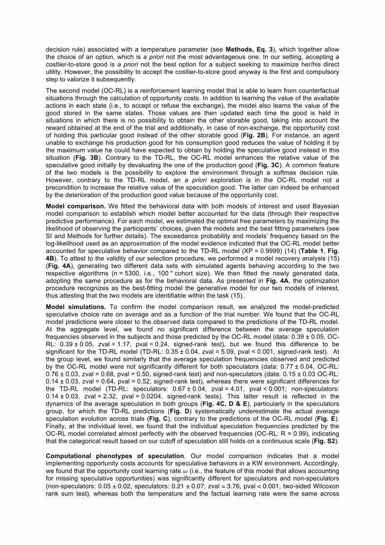
decision rule) associated with a temperature parameter (see Methods, Eq. 3), which together allow the choice of an option, which is a priori not the most advantageous one. In our setting, accepting a costlier-to-store good is a priori not the best option for a subject seeking to maximize her/his direct utility. However, the possibility to accept the costlier-to-store good anyway is the first and compulsory step to valorize it subsequently.

The second model (OC-RL) is a reinforcement learning model that is able to learn from counterfactual situations through the calculation of opportunity costs. In addition to learning the value of the available actions in each state (i.e., to accept or refuse the exchange), the model also learns the value of the good stored in the same states. Those values are then updated each time the good is held in situations in which there is no possibility to obtain the other storable good, taking into account the reward obtained at the end of the trial and additionally, in case of non-exchange, the opportunity cost of holding this particular good instead of the other storable good (Fig. 2B). For instance, an agent unable to exchange his production good for his consumption good reduces the value of holding it by the maximum value he could have expected to obtain by holding the speculative good instead in this situation (Fig. 3B). Contrary to the TD-RL, the OC-RL model enhances the relative value of the speculative good initially by devaluating the one of the production good (Fig. 3C). A common feature of the two models is the possibility to explore the environment through a softmax decision rule. However, contrary to the TD-RL model, an a priori exploration is in the OC-RL model not a precondition to increase the relative value of the speculation good. The latter can indeed be enhanced by the deterioration of the production good value because of the opportunity cost.

Model comparison. We fitted the behavioral data with both models of interest and used Bayesian model comparison to establish which model better accounted for the data (through their respective predictive performance). For each model, we estimated the optimal free parameters by maximizing the likelihood of observing the participants’ choices, given the models and the best fitting parameters (see SI and Methods for further details). The exceedance probability and models’ frequency based on the log-likelihood used as an approximation of the model evidence indicated that the OC-RL model better accounted for speculative behavior compared to the TD-RL model (XP = 0.9999) (14) (Table 1, Fig. 4B). To attest to the validity of our selection procedure, we performed a model recovery analysis (15) (Fig. 4A), generating two different data sets with simulated agents behaving according to the two respective algorithms (n = 5300, i.e., 100 * cohort size). We then fitted the newly generated data, adopting the same procedure as for the behavioral data. As presented in Fig. 4A, the optimization procedure recognizes as the best-fitting model the generative model for our two models of interest, thus attesting that the two models are identifiable within the task (15).

Model simulations. To confirm the model comparison result, we analyzed the model-predicted speculative choice rate on average and as a function of the trial number. We found that the OC-RL model predictions were closer to the observed data compared to the predictions of the TD-RL model. At the aggregate level, we found no significant difference between the average speculation frequencies observed in the subjects and those predicted by the OC-RL model (data: 0.39 ± 0.05, OC-RL: 0.39 ± 0.05, zval = 1.17, pval = 0.24, signed-rank test), but we found this difference to be significant for the TD-RL model (TD-RL: 0.35 ± 0.04, zval = 5.09, pval < 0.001, signed-rank test). At the group level, we found similarly that the average speculation frequencies observed and predicted by the OC-RL model were not significantly different for both speculators (data: 0.77 ± 0.04, OC-RL: 0.76 ± 0.03, zval = 0.68, pval = 0.50, signed-rank test) and non-speculators (data: 0.15 ± 0.03 OC-RL: 0.14 ± 0.03, zval = 0.64, pval = 0.52, signed-rank test), whereas there were significant differences for the TD-RL model (TD-RL: speculators: 0.67 ± 0.04, zval = 4.01, pval < 0.001; non-speculators: 0.14 ± 0.03, zval = 2.32, pval = 0.0204, signed-rank tests). This latter result is reflected in the dynamics of the average speculation in both groups (Fig. 4C, D & E), particularly in the speculators group, for which the TD-RL predictions (Fig. D) systematically underestimate the actual average speculation evolution across trials (Fig. C), contrary to the predictions of the OC-RL model (Fig. E). Finally, at the individual level, we found that the individual speculation frequencies predicted by the OC-RL model correlated almost perfectly with the observed frequencies (OC-RL: R = 0.99), indicating that the categorical result based on our cutoff of speculation still holds on a continuous scale (Fig. S2). Computational phenotypes of speculation. Our model comparison indicates that a model implementing opportunity costs accounts for speculative behaviors in a KW environment. Accordingly, we found that the opportunity cost learning rate 𝜔 (i.e., the feature of this model that allows accounting for missing speculative opportunities) was significantly different for speculators and non-speculators (non-speculators: 0.05 ± 0.02, speculators: 0.21 ± 0.07, zval = 3.76, pval < 0.001, two-sided Wilcoxon rank sum test), whereas both the temperature and the factual learning rate were the same across

groups (temperature: non-speculators: 0.11 ± 0.04, speculators: 0.18 ± 0.06, zval = 0.68, pval = 0.50; learning rate: non-speculators: 0.26 ± 0.05, speculators: 0.24 ± 0.07, zval = 1.35, pval = 0.18, two-sided Wilcoxon rank sum tests) (Fig. 4F). Thus, the relative account of opportunity costs in the agents' value estimation process through the counterfactual learning rate 𝜔 seems to be the key feature to understand and predict both speculative and non-speculative behaviors in the KW environment. The more the opportunity costs are accounted for (i.e., the greater 𝜔 is), the more striking the advantage of the speculative strategy.

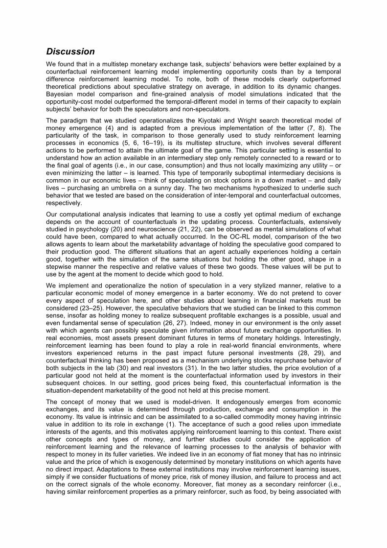
Discussion

We found that in a multistep monetary exchange task, subjects' behaviors were better explained by a counterfactual reinforcement learning model implementing opportunity costs than by a temporal difference reinforcement learning model. To note, both of these models clearly outperformed theoretical predictions about speculative strategy on average, in addition to its dynamic changes. Bayesian model comparison and fine-grained analysis of model simulations indicated that the opportunity-cost model outperformed the temporal-different model in terms of their capacity to explain subjects’ behavior for both the speculators and non-speculators.

The paradigm that we studied operationalizes the Kiyotaki and Wright search theoretical model of money emergence (4) and is adapted from a previous implementation of the latter (7, 8). The particularity of the task, in comparison to those generally used to study reinforcement learning processes in economics (5, 6, 16–19), is its multistep structure, which involves several different actions to be performed to attain the ultimate goal of the game. This particular setting is essential to understand how an action available in an intermediary step only remotely connected to a reward or to the final goal of agents (i.e., in our case, consumption) and thus not locally maximizing any utility – or even minimizing the latter – is learned. This type of temporarily suboptimal intermediary decisions is common in our economic lives – think of speculating on stock options in a down market – and daily lives – purchasing an umbrella on a sunny day. The two mechanisms hypothesized to underlie such behavior that we tested are based on the consideration of inter-temporal and counterfactual outcomes, respectively.

Our computational analysis indicates that learning to use a costly yet optimal medium of exchange depends on the account of counterfactuals in the updating process. Counterfactuals, extensively studied in psychology (20) and neuroscience (21, 22), can be observed as mental simulations of what could have been, compared to what actually occurred. In the OC-RL model, comparison of the two allows agents to learn about the marketability advantage of holding the speculative good compared to their production good. The different situations that an agent actually experiences holding a certain good, together with the simulation of the same situations but holding the other good, shape in a stepwise manner the respective and relative values of these two goods. These values will be put to use by the agent at the moment to decide which good to hold.

We implement and operationalize the notion of speculation in a very stylized manner, relative to a particular economic model of money emergence in a barter economy. We do not pretend to cover every aspect of speculation here, and other studies about learning in financial markets must be considered (23–25). However, the speculative behaviors that we studied can be linked to this common sense, insofar as holding money to realize subsequent profitable exchanges is a possible, usual and even fundamental sense of speculation (26, 27). Indeed, money in our environment is the only asset with which agents can possibly speculate given information about future exchange opportunities. In real economies, most assets present dominant futures in terms of monetary holdings. Interestingly, reinforcement learning has been found to play a role in real-world financial environments, where investors experienced returns in the past impact future personal investments (28, 29), and counterfactual thinking has been proposed as a mechanism underlying stocks repurchase behavior of both subjects in the lab (30) and real investors (31). In the two latter studies, the price evolution of a particular good not held at the moment is the counterfactual information used by investors in their subsequent choices. In our setting, good prices being fixed, this counterfactual information is the situation-dependent marketability of the good not held at this precise moment.

The concept of money that we used is model-driven. It endogenously emerges from economic exchanges, and its value is determined through production, exchange and consumption in the economy. Its value is intrinsic and can be assimilated to a so-called commodity money having intrinsic value in addition to its role in exchange (1). The acceptance of such a good relies upon immediate interests of the agents, and this motivates applying reinforcement learning to this context. There exist other concepts and types of money, and further studies could consider the application of reinforcement learning and the relevance of learning processes to the analysis of behavior with respect to money in its fuller varieties. We indeed live in an economy of fiat money that has no intrinsic value and the price of which is exogenously determined by monetary institutions on which agents have no direct impact. Adaptations to these external institutions may involve reinforcement learning issues, simply if we consider fluctuations of money price, risk of money illusion, and failure to process and act on the correct signals of the whole economy. Moreover, fiat money as a secondary reinforcer (i.e., having similar reinforcement properties as a primary reinforcer, such as food, by being associated with

the latter) has been repeatedly evidenced in appetitive (32, 33) and aversive conditioning (34, 35). In this sense, our study shed some light on the process by which a type of money ‘in the making’ acquires this secondary reinforcing property through strategic interactions and the cognitive traits underlying this process. The fact that both primary and secondary reinforcers have been found to rely on overlapping neural regions (36) raises an intriguing question that could be addressed in a future study dedicated to exploring whether the reward-related neural activity from using a speculative medium of exchange evolves in speculators toward an overlapping of the neural representation of the latter and the one of the consumption good.

An important aspect of our results is the inter-individual variability regarding the use of this speculative commodity money. Both groups of subjects were found to learn over time to adopt it, or on the contrary, to reject it. This aspect is reminiscent of Carl Menger in "On the origin of money" (1892):

“Nothing may have been so favorable to the genesis of a medium of exchange as the acceptance, on the part of the most discerning and capable economic subjects, for their own economic gain, of eminently saleable goods in preference to all others.”

Speculators in our experiments would refer to those particularly discerning subjects, extracting from their experience the relatively high saleability of the speculative good. Our computational results tend to indicate that this variability relies on the integration of counterfactual outcomes in the value-updating process.

A limitation of our study concerns the generalizability of the OC-RL model. In its current form, the OC-RL model would not be easily transferable to other tasks because of its tight adequacy to the specific structure of the money emergence paradigm. Particularly, the algorithm distinguishes between two types of states, those in which the agent can decide which good to hold in the next step and those in which he does not have such a choice, and this feature is characteristic of the operationalized KW environment that we used. In this sense, the OC-RL model lies between model-free algorithms that learn by trial and error and model-based algorithms that make use of the structure of the task to make decisions (37, 38). Generally, model-based algorithms involve the acquisition of a "cognitive map" of the task (38, 39), describing how different states are connected and agents learn, through state-prediction-error, these state transitions. Whereas the OC-RL model neither knows nor learns the full task structure, it is able to differentiate some states from others. Few adjustments would then be needed to adapt the OC-RL model to other tasks. The counterfactual feedback processing per se is highly flexible and adaptable while permitting a richer knowledge of the learning environment (40).

Although the OC-RL model outperforms the TD-RL models in terms of its predictive power at the population level, this result does not mean that inter-temporal valuation of future rewards is totally irrelevant in the process of learning to speculate and that no subject implemented this computational process to account for these rewards instead of or in addition to the counterfactual learning of opportunity costs. Further studies would be necessary to clarify the possible interaction between the two processes, and one can easily envision a hybrid model that accounts for both types of reward simultaneously, at the price, though, of greater computational complexity.

MaterialsandMethodsSample. Our sample included 53 healthy subjects (30 females and 23 males between the ages of 20 and 41 years old, with a median age of 24 years old). The participants earned a fixed amount of money (10€) for their participation and had the possibility to double this amount according to their performance. Indeed, 20 consecutive trials were drawn, and the total number of points accumulated in those 20 rounds was transformed into a probability of winning the extra 10€. The experimental protocol was in accordance with experimental economics standards such that subjects were perfectly informed about the economic game functioning and the remuneration rules (i.e., there was no deception throughout the experimental process).

Behavioral Task. The exchange task is based on the Kiyotaki and Wright model of money emergence (4) and adapted with a few slight variations from a previous implementation of the model (7, 8).

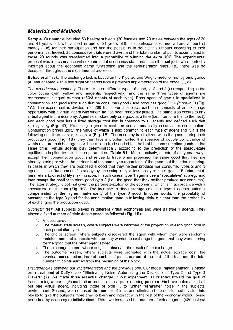
The experimental economy. There are three different types of good, 1, 2 and 3 (corresponding to the color codes cyan, yellow and magenta, respectively), and the same three types of agents are represented in equal number (480/3 agents of each type). Each agent of type 𝑖 is specialized in consumption and production such that he consumes good 𝑖 and produces good (modulo 3) (Fig. 1A). The experiment is divided into 200 trials. For a subject, each trial consists of an exchange opportunity with a virtual agent with whom he has been randomly paired. The same also occurs to any virtual agent in the economy. Agents can store only one good at a time (i.e., from one trial to the next), and each good type has a fixed storage cost that is common to all agents and defined such that 𝑐! < 𝑐! < 𝑐! (Fig. 1D). Producing a good is cost-free and automatically occurs after consumption. Consumption brings utility, the value of which is also common to each type of agent and fulfills the following condition: 𝑐! < 𝑐! < 𝑐! < 𝑢 (Fig. 1E). The economy is initialized with all agents storing their production good (Fig. 1B); they then face a problem called the absence of double coincidence of wants (i.e., no matched agents will be able to trade and obtain both of their consumption goods at the same time). Virtual agents play deterministically according to the prediction of the steady-state equilibrium implied by the chosen parameters (Table S1). More precisely, agents of all types always accept their consumption good and refuse to trade when proposed the same good that they are already storing or when the partner is of the same type regardless of the good that the latter is storing. In cases in which they are proposed a good that they neither produce nor consume, types 2 and 3 agents use a "fundamental" strategy by accepting only a less-costly-to-store good. "Fundamental" here refers to direct utility maximization. In such cases, type 1 agents use a "speculative" strategy and then accept the costlier-to-store good type 3 (i.e., the good that they neither produce nor consume). The latter strategy is optimal given the parameterization of the economy, which is in accordance with a speculative equilibrium (Fig. 1C). The increase in direct storage cost that type 1 agents suffer is compensated by the higher marketability of the type 3 good. In other words, the probability of exchanging the type 3 good for the consumption good in following trials is higher than the probability of exchanging the production good.

Subjects’ task. All subjects played in different virtual economies and were all type 1 agents. They played a fixed number of trials decomposed as followed (Fig. 1E):

1. A focus screen. 2. The market state screen, where subjects were informed of the proportion of each good type in

each population type. 3. The choice screen, where subjects discovered the agent with whom they were randomly

matched and had to decide whether they wanted to exchange the good that they were storing for the good that the other agent stored.

4. The exchange screen, where subjects observed the result of the exchange. 5. The outcome screen, where subjects were prompted with the actual storage cost, the

eventual consumption, the net number of points earned at the end of the trial, and the total number of points earned from the beginning of the block.

Discrepancies between our implementation and the previous one. Our model implementation is based on a treatment of Duffy's task "Eliminating Noise: Automating the Decisions of Type 2 and Type 3 Players" (7). We made three essential changes in our experiment, all oriented toward the goal of transforming a learning/coordination problem into a pure learning problem. First, we automatized all but one virtual agent, including those of type 1, to further "eliminate" noise in the subjects' environment. Second, we increased the number of trials and eliminated the session subdivision into blocks to give the subjects more time to learn and interact with the rest of the economy without being perturbed by economy re-initializations. Third, we increased the number of virtual agents (480 instead

of a maximum of 24 previously) to standardize and stabilize the proportions of each types of good stored by each type of agent. This modification allowed the virtual economy to run much closer to the equilibrium predictions (Fig. S1).

Computational Modeling. We fitted the data with two reinforcement learning models: a temporal difference model (TD-RL) and an opportunity costs model (OC-RL). The model space included then the standard Q-learning model originally introduced by Watkins (10–12) and a newly designed reinforcement learning model based on opportunity costs. The models are described under the perspective of type 1 agent modeling, the only agent type in which we are interested in this study.

Q-Learning model (TD-RL). This model is a classic off-policy reinforcement learning model. For each exchange situation (characterized by the stored goods' type, the proposed goods' type and the partner's type), the model estimates the expected choices and outcomes. These Q-values essentially represent the expected reward obtained by taking a particular option in a given context, here, the exchange of the stored good for the proposed good and the non-exchange of this good. In both experiments, Q-values were set for all situations, in accordance with the goods' costs and utility. The action value of refusing an exchange was set equal to the cost of the good stored at the moment of exchange. The action value of accepting an exchange was set to the net utility of the proposed good (i.e., the utility that it eventually provides in case of consumption minus the cost of the good to be stored until the next round). These priors on the initial Q-values are based on the fact that subjects were explicitly informed in the instructions about the different storing costs and the utility value of consumption. After every trial 𝑡, the value of the chosen option 𝑎! ("accepting the exchange" or "refusing the exchange", henceforth, 𝑎𝑐𝑐𝑒𝑝𝑡 and 𝑟𝑒𝑓𝑢𝑠𝑒, respectively) in the state 𝑠! is updated according to the following rule:

where is the prediction error and calculated as

𝛿! = 𝑟! + 𝛾 max!!!!∈𝒜

𝑄! 𝑠!!!, 𝑎!!! − 𝑄! 𝑠! , 𝑎! # 2

where 𝑟! is the reward obtained as an outcome of choosing 𝑎! in the state 𝑠! and max!!!!∈𝒜 𝑄! 𝑠!!!, 𝑎!!! the maximum of the action values of the 𝑡 + 1 state. In other words, the prediction error is the difference between the expected reward 𝑄! 𝑠! , 𝑎! and the actual reward

. The reward magnitude range is [-0.09; 0.96], from the net utility of the costlier-to-store good to the net utility of the consumption good. The learning rate, 𝛼, is a scaling parameter that adjusts the amplitude of value changes from one trial to the next, and the discount factor, 𝛾, is a scaling parameters that adjust the value of future outcomes. Following this rule, option values are increased if the outcome is better than expected and decreased in the opposite case, and the amplitude of the update is similar following positive and negative prediction errors. Finally, given the Q-values, the associated probability (or likelihood) of selecting each option is estimated by implementing the softmax decision rule for choosing accept, which is as follows:

𝑃! 𝑠! , 𝑎𝑐𝑐𝑒𝑝𝑡 =𝑒! !!,!""#$%

!

𝑒!! !!,!""#$%

! + 𝑒!! !!,!"#$%"

!

# 3

This rule is a standard stochastic decision rule that calculates the probability of selecting one of a set of options according to their associated values. The temperature, 𝛽, is another scaling parameter that adjusts the stochasticity of decision-making and by doing so controls the exploration–exploitation trade-off.

The Opportunity Costs Reinforcement-Learning model (OC-RL model). This model is a model-based reinforcement learning model that we developed to implement opportunity costs within a reinforcement learning process. It has been inspired in its integration of opportunity costs by a half-deterministic half-reinforcement learning model previously presented to explain speculative behaviors in a KW environment (7). It distinguishes two types of exchange situations in the KW environment. The first type corresponds to situations in which an agent has the opportunity to exchange the good that he is storing for another storable good (type 1 agents can store only types 2 and 3 goods; the first type of situations concerns exchanges involving those two goods). In such situations, agents decide what type of good they prefer holding. The second type corresponds to situations in which the agent has the opportunity to exchange the good that he is storing for his consumption good or a same-type good.

They then constitute the experience the agent has with the good that he is storing. The experience is positive when he is able to consume and negative when he has to wait another round to eventually consume. As implemented in the Q-learning, the values of actions (i.e., accept or reject the exchange) for each exchange situation take the form of Q-values, updated according to two distinct learning rules depending on the situation types described above.

In the "experience" situations (second type), the Q-values are updated with the same rule as they are in the q-learning model (eq. 1), but the prediction error is differently defined in the sense that it does not include future rewards (i.e., 𝛾 = 0). The predictions error becomes

𝛿! = 𝑟! − 𝑄! 𝑠!! , 𝑎! # 4

The agent is thus myopic regarding future rewards attainable in following states. Note that the notation

of states in the OC-RL model includes a specification about which good is held in this state, .

In the "storing good choice" situations (first type), only two values are used for all situations, the value of holding good 2 and the value of holding good 3. Those values are computed and updated in the "experience" situations according to a principle of classical conditioning and including opportunity costs. Each time that an agent receives an outcome from a choice in the "experience" situations, he updates not only the Q-value of the corresponding choice as previously described but also the value of holding the good that he had in storage at the beginning of the trial. For instance, if a type 1 agent holds a type 2 good, accepts to exchange it for his consumption good, and is successful at doing so, he updates the Q-value of the action "accept" in this situation and the value of holding the type 2 good in general. Now, to implement opportunity costs, two cases must be defined. The first is the case of a realized exchange (i.e., when both matched agents mutually agree on it), in which the held good value is updated with the same rule used for actions' Q-value in "experience" situations (eq. 1) and with a similar prediction error calculation:

𝛿! = 𝑟! − 𝑉!(𝑔!)# 5

where 𝑉!(𝑔!) is the value of the good hold at the beginning of the round. Note that the same learning rate 𝛼 is used here as the information concerned actual outcomes. A second learning rate 𝜔 for "counterfactual" information is introduced below.

The second case concerns unrealized exchanges in which the value of the good held at the beginning of the trial is updated in a similar manner but with a second learning rate 𝜔 and a prediction error including opportunity costs. The updating rule is then

𝑉!!!(𝑔!) = 𝑉!(𝑔!) + 𝜔𝛿′!# 6

with 𝛿′! calculated as follows:

𝛿′! = 𝑟! − 𝑂𝐶!(𝑔!) − 𝑉!(𝑔!)# 7

where 𝑂𝐶!(𝑔!) is the opportunity cost of holding good ℎ instead of −ℎ and equals

𝑂𝐶!(𝑔!) = max!!∈𝒜

𝑄! 𝑠!!! , 𝑎! # 8

where is the maximum value expected from choosing action 𝑎 in the same situation but holding −ℎ instead of ℎ.

We implemented the same decision rule as for the Q-learning, namely, a softmax policy. For choice in "experience" situations, the equation is the same as before (eq. 3), whereas for "storing good choice" situations, the equation becomes

Model Comparison.

We optimized the model parameters by minimizing the negative log-likelihood of the data given different parameters settings using Matlab’s 𝑓𝑚𝑖𝑛𝑐𝑜𝑛 function, as previously described (41). Parameter recovery analyses based on model simulations show that our parameter optimization procedure and model selection correctly retrieves the generating model as the wining model (Fig. 2A

and Fig. 3A). Note that as our two models of interest have the same number of degrees of freedom (i.e., 3 free parameters each), we did not have to take into account their complexity in the model comparison when calculating the Bayesian and Akaike information criterion. Individual negative log-likelihoods values were fed into 𝑚𝑏𝑏 − 𝑣𝑏 − 𝑡𝑜𝑜𝑙𝑏𝑜𝑥 (14), a procedure that estimates the expected frequencies and the exceedance probability for each model within a set of models, given the data gathered from all participants. The exceedance probability (denoted XP) is the probability that a given model fits the data better than all other models in the set.

Acknowledgments SP is supported by an ATIP-Avenir grant (R16069JS), the Programme Emergence(s) de la Ville de Paris, and the Fyssen foundation. SP and SBJ are supported by a Collaborative Research in Computational Neuroscience ANR-NSF grant (ANR-16-NEUC-0004). The Institut d’Etude de la Cognition is supported financially by the LabEx IEC (ANR-10-LABX-0087 IEC) and the IDEX PSL* (ANR-10-IDEX-0001-02 PSL*).

References 1. Menger C (1892) The Origin of Money. Econ J 2:239–55.

2. Hicks JR (1935) A Suggestion for Simplifying the Theory of Money. Economica 2(5):1–19.

3. Jones RA (1976) The Origin and Development of Media of Exchange. J Polit Econ 84(4):757–776.

4. Kiyotaki N, Wright R (1989) On Money as a Medium of Exchange. J Polit Econ 97(4):927–954.

5. Roth AE, Erev I (1995) Learning in extensive-form games: Experimental data and simple dynamic models in the intermediate term. Games Econ Behav 8(1):164–212.

6. Ido Erev, Roth AE (1998) Predicting how people play games: Reinforcement learning in experimental games with unique, mixed strategy equilibria. Am Econ Rev 88(4):848–881.

7. Duffy J (2001) Learning to speculate: Experiments with artificial and real agents. J Econ Dyn Control 25(3–4):295–319.

8. Duffy J, Ochs J (1999) Emergence of Money as a Medium of Exchange: An Experimental Study. Am Econ Rev 89(4):847–877.

9. Brown PM (1996) Experimental evidence on money as a medium of exchange. J Econ Dyn Control 20(4):583–600.

10. Watkins CJCH (1989) Learning from Delayed Rewards. Dissertation (Cambridge University).

11. Watkins CJCH, Dayan P (1992) Technical Note: Q-Learning. Mach Learn 8(3):279–292.

12. Sutton RS, Barto AG (1998) Introduction to Reinforcement Learning doi:10.1.1.32.7692.

13. Watkins CJCH, Dayan P (1992) Q-learning. Mach Learn 8(3–4):279–292.

14. Daunizeau J, Adam V, Rigoux L (2014) VBA�: A Probabilistic Treatment of Nonlinear Models for Neurobiological and Behavioural Data. PLoS Comput Biol 10(1):e1003441.

15. Palminteri S, Wyart V, Koechlin E (2017) The Importance of Falsification in Computational Cognitive Modeling. Trends Cogn Sci 21(6):425–433.

16. Arthur B (1991) Designing Economic Agents That Act Like Human Agents: A Behavioral Approach to Bounded Rationality. Am Econ Rev 81(2):353–359.

17. Bereby-Meyer Y, Erev I (1998) On Learning To Become a Successful Loser: A Comparison of Alternative Abstractions of Learning Processes in the Loss Domain. J Math Psychol 42(2–3):266–286.

18. Erev I, Bereby-Meyer Y, Roth AE (1999) The effect of adding a constant to all payoffs: Experimental investigation, and implications for reinforcement learning models. J Econ Behav Organ 39(1):111–128.

19. Horita Y, Takezawa M, Inukai K, Kita T, Masuda N (2017) Reinforcement learning accounts for moody conditional cooperation behavior: experimental results. Sci Rep 7.

doi:10.1038/srep39275.

20. Byrne RMJ (2016) Counterfactual Thought. Annu Rev Psychol 67(1):135–157.

21. Camille N, et al. (2004) The involvement of the orbitofrontal cortex in the experience of regret. Science (80- ) 304(5674):1167–1170.

22. Coricelli G, et al. (2005) Regret and its avoidance: A neuroimaging study of choice behavior. Nat Neurosci 8(9):1255–1262.

23. Pastor L, Veronesi P (2009) Learning in Financial Markets. Annu Rev Financ Econ 1(1):361–381.

24. Seru A, Shumway T, Stoffman N (2010) Learning by trading. Rev Financ Stud 23(2):705–739.

25. Gervais S, Odean T (2001) Learning to be overconfident. Rev Financ Stud 14(1):1–27.

26. Kaldor N (1939) Speculation and Economic Stability. Rev Econ Stud 7(1):1–27.

27. Feiger G (1976) What is Speculation? Q J Econ 90(4):677–687.

28. Kaustia M, Knüpfer S (2008) Do investors overweight personal experience? evidence from IPO subscriptions. J Finance 63(6):2679–2702.

29. Choi JJ, Laibson D, Madrian BC, Metrick A (2009) Reinforcement learning and savings behavior. J Finance 64(6):2515–2534.

30. Weber M, Welfens F (2011) The follow-on purchase and repurchase behavior of individual investors: An experimental investigation. Die Betriebswirtschaft 71(2):139–154.

31. Strahilevitz MA, Odean T, Barber BM (2011) Once Burned, Twice Shy: How Naive Learning, Counterfactuals, and Regret Affect the Repurchase of Stocks Previously Sold. J Mark Res 48(SPL):S102–S120.

32. Valentin V V., O’Doherty JP (2009) Overlapping Prediction Errors in Dorsal Striatum During Instrumental Learning With Juice and Money Reward in the Human Brain. J Neurophysiol 102(6):3384–3391.

33. Kim H, Shimojo S, O’Doherty JP (2011) Overlapping responses for the expectation of juice and money rewards in human ventromedial prefrontal cortex. Cereb Cortex 21(4):769–776.

34. Delgado MR, Labouliere CD, Phelps EA (2006) Fear of losing money? Aversive conditioning with secondary reinforcers. Soc Cogn Affect Neurosci 1(3):250–259.

35. Delgado MR, Jou RL, Phelps EA (2011) Neural systems underlying aversive conditioning in humans with primary and secondary reinforcers. Front Neurosci (MAY). doi:10.3389/fnins.2011.00071.

36. Sescousse G, Redoute J, Dreher J-C (2010) The Architecture of Reward Value Coding in the Human Orbitofrontal Cortex. J Neurosci 30(39):13095–13104.

37. Daw ND, Niv Y, Dayan P (2005) Uncertainty-based competition between prefrontal and dorsolateral striatal systems for behavioral control. Nat Neurosci 8(12):1704–1711.

38. Gläscher J, Daw N, Dayan P, O’Doherty JP (2010) States versus rewards: Dissociable neural prediction error signals underlying model-based and model-free reinforcement learning. Neuron 66(4):585–595.

39. Tolman EC (1948) Cognitive maps in rats and men. Psychol Rev 55(4):189–208.

40. Lohrenz T, McCabe K, Camerer CF, Montague PR (2007) Neural signature of fictive learning signals in a sequential investment task. Proc Natl Acad Sci 104(22):9493–9498.

41. Palminteri S, Khamassi M, Joffily M, Coricelli G (2015) Contextual modulation of value signals in reward and punishment learning. Nat Commun 6:8096.

Figures

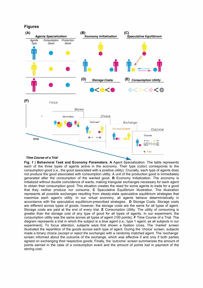
Fig. 1 | Behavioral Task and Economy Parameters. A Agent Specialization. The table represents each of the three types of agents active in the economy. Their type (color) corresponds to the consumption good (i.e., the good associated with a positive utility). Crucially, each type of agents does not produce the good associated with consumption utility. A unit of the production good is immediately generated after the consumption of the wanted good. B Economy Initialization. The economy is initialized without double coincidence of wants, making triangular exchanges necessary for each agent to obtain their consumption good. This situation creates the need for some agents to trade for a good that they neither produce nor consume. C Speculative Equilibrium Illustration. The illustration represents all possible exchanges resulting from steady-state speculative equilibrium strategies that maximize each agent’s utility. In our virtual economy, all agents behave deterministically in accordance with the speculative equilibrium-prescribed strategies. D Storage Costs. Storage costs are different across types of goods; however, the storage costs are the same for all types of agent. Storage costs are paid at the end of every trial. E Consumption Utility. The utility of consuming is greater than the storage cost of any type of good for all types of agents. In our experiment, the consumption utility was the same across all types of agent (100 points). F Time Course of a Trial. The diagram represents a trial in which the subject is a blue agent (i.e., type 1 agent, as all subjects in our experiment). To focus attention, subjects were first shown a fixation cross. The ‘market’ screen illustrated the repartition of the goods across each type of agent. During the ‘choice’ screen, subjects made a binary choice (accept or reject the exchange) with a randomly matched agent. The ‘exchange’ screen informed about the outcome of the exchange, which was effective if and only if both parties agreed on exchanging their respective goods. Finally, the ‘outcome’ screen summarizes the amount of points earned in the case of a consumption event and the amount of points lost in payment of the storing cost.

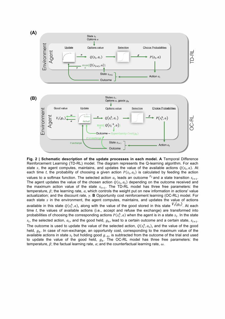
Fig. 2 | Schematic description of the update processes in each model. A Temporal Difference Reinforcement Learning (TD-RL) model. The diagram represents the Q-learning algorithm. For each state 𝑠, the agent computes, maintains, and updates the value of the available actions 𝑄 𝑠! , 𝑎 . At each time t, the probability of choosing a given action 𝑃 𝑠! , 𝑎! is calculated by feeding the action values to a softmax function. The selected action 𝑎! leads an outcome and a state transition 𝑠!!!. The agent updates the value of the chosen action 𝑄 𝑠! , 𝑎! depending on the outcome received and the maximum action value of the state 𝑠!!!. The TD-RL model has three free parameters: the temperature, 𝛽; the learning rate, 𝛼, which controls the weight put on new information in actions' value actualization; and the discount rate, 𝛾. B Opportunity cost reinforcement learning (OC-RL) model. For each state 𝑠 in the environment, the agent computes, maintains, and updates the value of actions available in this state 𝑄 𝑠!! , 𝑎 , along with the value of the good stored in this state . At each time t, the values of available actions (i.e., accept and refuse the exchange) are transformed into probabilities of choosing the corresponding actions 𝑃 𝑠!! , 𝑎 when the agent is in a state 𝑠!. In the state 𝑠!, the selected action, 𝑎!, and the good held, 𝑔!, lead to a certain outcome and a certain state, 𝑠!!!. The outcome is used to update the value of the selected action, 𝑄 𝑠!! , 𝑎! , and the value of the good held, 𝑔!. In case of non-exchange, an opportunity cost, corresponding to the maximum value of the available actions in state 𝑠! but holding good 𝑔!!, is subtracted from the outcome of the trial and used to update the value of the good held, 𝑔!. The OC-RL model has three free parameters: the temperature, 𝛽; the factual learning rate, 𝛼; and the counterfactual learning rate, 𝜔.

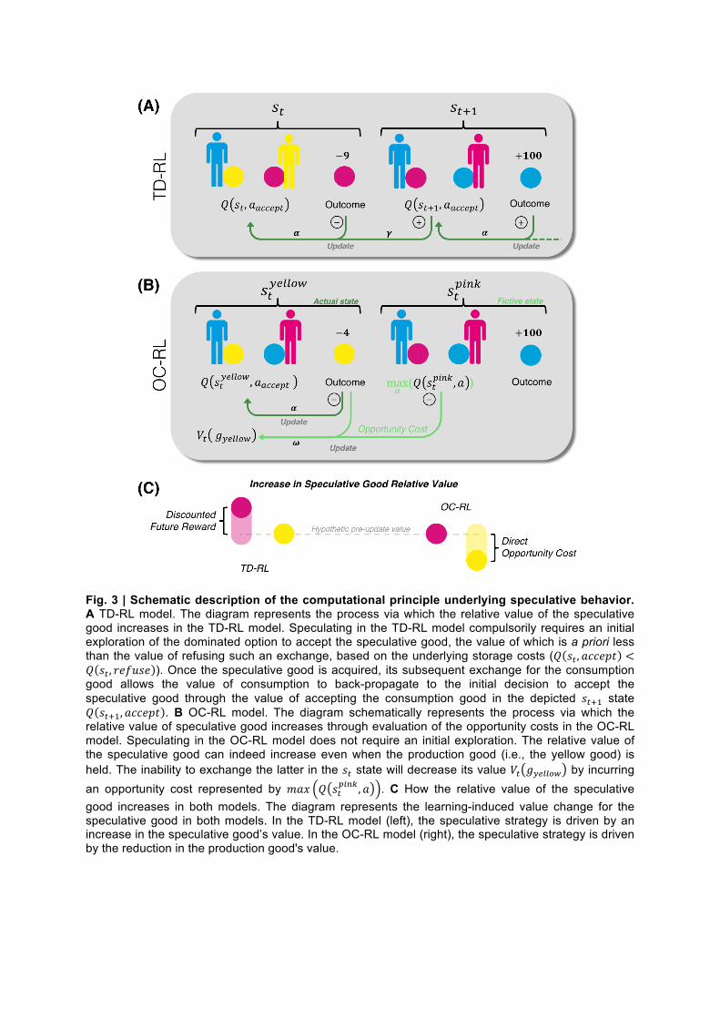
Fig. 3 | Schematic description of the computational principle underlying speculative behavior. A TD-RL model. The diagram represents the process via which the relative value of the speculative good increases in the TD-RL model. Speculating in the TD-RL model compulsorily requires an initial exploration of the dominated option to accept the speculative good, the value of which is a priori less than the value of refusing such an exchange, based on the underlying storage costs (𝑄 𝑠! , 𝑎𝑐𝑐𝑒𝑝𝑡 <𝑄 𝑠! , 𝑟𝑒𝑓𝑢𝑠𝑒 ). Once the speculative good is acquired, its subsequent exchange for the consumption good allows the value of consumption to back-propagate to the initial decision to accept the speculative good through the value of accepting the consumption good in the depicted 𝑠!!! state 𝑄 𝑠!!!, 𝑎𝑐𝑐𝑒𝑝𝑡 . B OC-RL model. The diagram schematically represents the process via which the relative value of speculative good increases through evaluation of the opportunity costs in the OC-RL model. Speculating in the OC-RL model does not require an initial exploration. The relative value of the speculative good can indeed increase even when the production good (i.e., the yellow good) is held. The inability to exchange the latter in the 𝑠! state will decrease its value 𝑉! 𝑔!"##$% by incurring an opportunity cost represented by 𝑚𝑎𝑥 𝑄 𝑠!

!"#$ , 𝑎 . C How the relative value of the speculative good increases in both models. The diagram represents the learning-induced value change for the speculative good in both models. In the TD-RL model (left), the speculative strategy is driven by an increase in the speculative good’s value. In the OC-RL model (right), the speculative strategy is driven by the reduction in the production good's value.

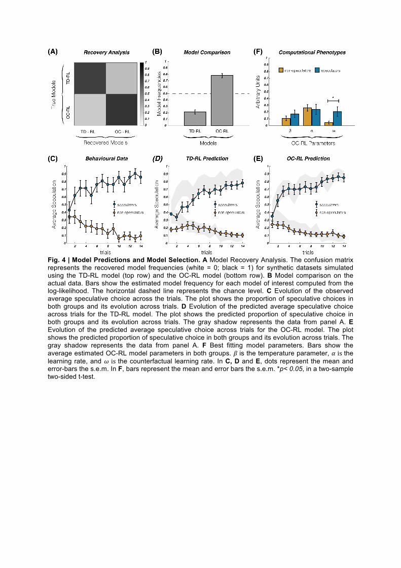
Fig. 4 | Model Predictions and Model Selection. A Model Recovery Analysis. The confusion matrix represents the recovered model frequencies (white = 0; black = 1) for synthetic datasets simulated using the TD-RL model (top row) and the OC-RL model (bottom row). B Model comparison on the actual data. Bars show the estimated model frequency for each model of interest computed from the log-likelihood. The horizontal dashed line represents the chance level. C Evolution of the observed average speculative choice across the trials. The plot shows the proportion of speculative choices in both groups and its evolution across trials. D Evolution of the predicted average speculative choice across trials for the TD-RL model. The plot shows the predicted proportion of speculative choice in both groups and its evolution across trials. The gray shadow represents the data from panel A. E Evolution of the predicted average speculative choice across trials for the OC-RL model. The plot shows the predicted proportion of speculative choice in both groups and its evolution across trials. The gray shadow represents the data from panel A. F Best fitting model parameters. Bars show the average estimated OC-RL model parameters in both groups. 𝛽 is the temperature parameter, 𝛼 is the learning rate, and 𝜔 is the counterfactual learning rate. In C, D and E, dots represent the mean and error-bars the s.e.m. In F, bars represent the mean and error bars the s.e.m. *p< 0.05, in a two-sample two-sided t-test.

Tables Optimization/ Model

LLmax XP MF

All Trials TD-RL 31.9 ± 2.8 0.0378 0.37 ± 0.05 OC-RL 31.6 ± 3.0 0.9722 0.63 ± 0.05 Speculation Only TD-RL 8.04 ± 0.84 0.0001 0.22 ± 0.03 OC-RL 6.81 ± 0.83 0.9999 0.78 ± 0.03

Table 1 | The table summarizes the fitting performances for each model. All Trials: the likelihood is calculated taking into account all trials. Speculation Only: the likelihood is calculated taking into account only the choice with an opportunity to speculate. LLmax, maximal log likelihood; XP, exceedance probability; MF, model frequency. Data are expressed as the mean ± s.e.m.

Data Overall First Opp. Last Opp. Observed Speculators 0.77 ± 0.04 0.43 ± 0.11 0.86 ± 0.08 Non-Speculators 0.15 ± 0.03 0.34 ± 0.09 0.09 ± 0.05 TD-RL Speculators 0.67 ± 0.04 0.38 ± 0.02 0.78 ± 0.05 Non-Speculators 0.14 ± 0.03 0.18 ± 0.03 0.10 ± 0.02 OC-RL Speculators 0.76 ± 0.03 0.35 ± 0.05 0.85 ± 0.05 Non-Speculators 0.14 ± 0.03 0.24 ± 0.04 0.09 ± 0.02

Table 2 | The table summarizes, for each group of subjects, the actual and predicted average speculation decision overall and at the first and last opportunities.

Supplementary Information

nAgents StoringCosts ConsumptionUtility Beta nTrial nBlock480 [1,4,9] 100 0.995 200 1

TableS1|Thetablesummarizestheparameterizationofthevirtualeconomy:"nAgents"thenumberofagentsintheeconomy,comprisingofn-1virtualagentsand1realsubject;"StoringCosts"thestoringcostsvaluefortype1,2and3goods(inoursetting,cyan,yellow,magenta)commonacrossallagents'types;"ConsumptionUtility"theutilityvalueofconsumptioncommonacrossallagents'types;"Beta"thediscountparameterusedtodeterminevirtualagentsstrategies;"nTrial"thetotalnumberoftrialsintheexperiments;"nBlock"thenumberofsubdivisionofthetotalnumberoftrials.

Fig.S1|TheoreticalEquilibriumintheExperimentalEconomy.Theplotshowstheevolutionofthethree steady-state equilibrium proportions of production good held by the three types of agents.Coloredlinesrepresenttheproportionforeachsubject'svirtualeconomyindividuallywhiletheblackthicklinerepresentstheaverageproportion.

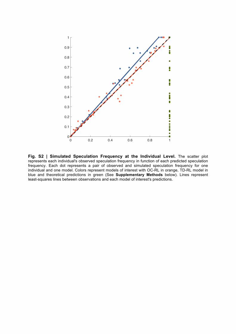
Fig. S2 | Simulated Speculation Frequency at the Individual Level. The scatter plot represents each individual's observed speculation frequency in function of each predicted speculation frequency. Each dot represents a pair of observed and simulated speculation frequency for one individual and one model. Colors represent models of interest with OC-RL in orange, TD-RL model in blue and theoretical predictions in green (See Supplementary Methods below). Lines represent least-squares lines between observations and each model of interest's predictions.

0 0.2 0.4 0.6 0.8 10

0.1

0.2

0.3

0.4

0.5

0.6

0.7

0.8

0.9

1

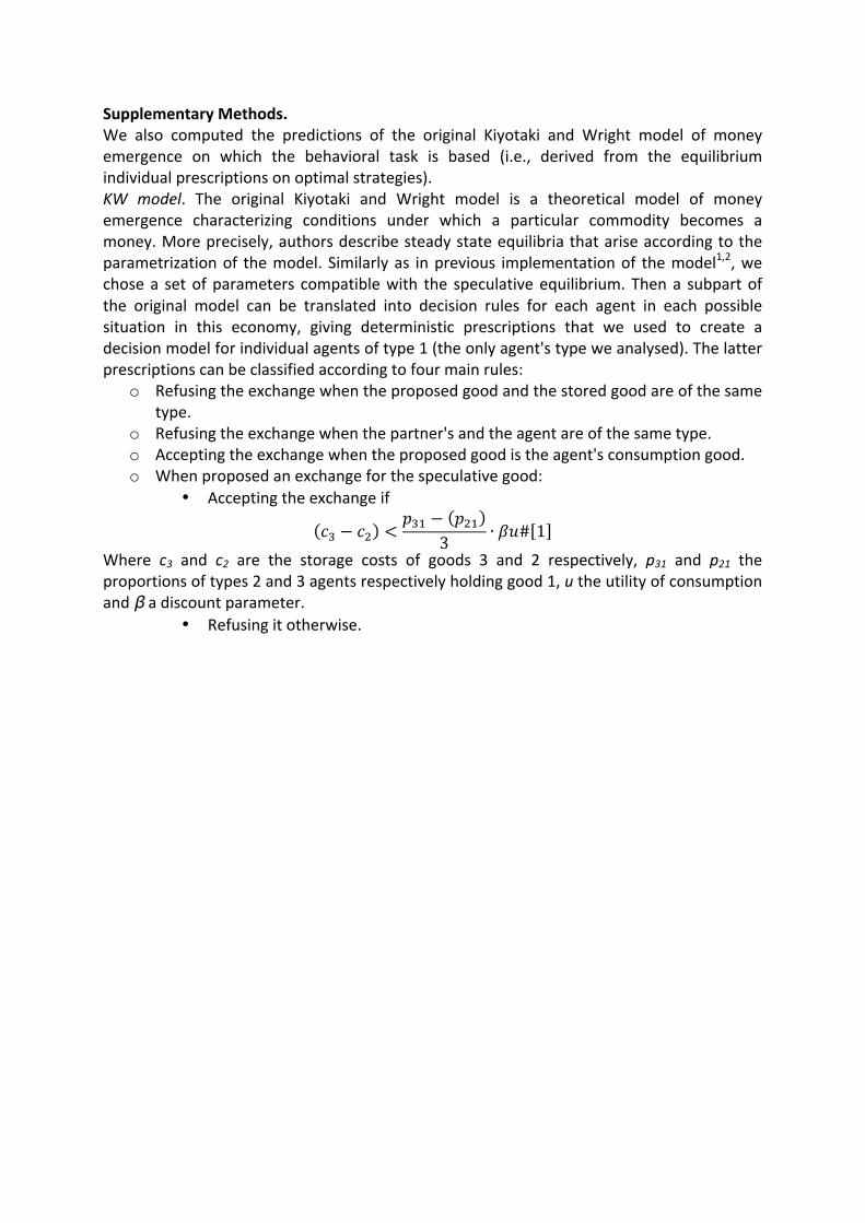
SupplementaryMethods.We also computed the predictions of the original Kiyotaki and Wright model of moneyemergence on which the behavioral task is based (i.e., derived from the equilibriumindividualprescriptionsonoptimalstrategies).KW model. The original Kiyotaki and Wright model is a theoretical model of moneyemergence characterizing conditions under which a particular commodity becomes amoney.Moreprecisely,authorsdescribesteadystateequilibriathatariseaccordingtotheparametrizationof themodel. Similarlyas inprevious implementationof themodel1,2,wechosea setofparameters compatiblewith the speculativeequilibrium.Thena subpartofthe original model can be translated into decision rules for each agent in each possiblesituation in this economy, giving deterministic prescriptions that we used to create adecisionmodelforindividualagentsoftype1(theonlyagent'stypeweanalysed).Thelatterprescriptionscanbeclassifiedaccordingtofourmainrules:

o Refusingtheexchangewhentheproposedgoodandthestoredgoodareofthesametype.

o Refusingtheexchangewhenthepartner'sandtheagentareofthesametype.o Acceptingtheexchangewhentheproposedgoodistheagent'sconsumptiongood.o Whenproposedanexchangeforthespeculativegood:

• Acceptingtheexchangeif

𝑐! − 𝑐! <𝑝!" − 𝑝!"

3∙ 𝛽𝑢# 1

Where c3 and c2 are the storage costs of goods 3 and 2 respectively, p31 and p21 theproportionsoftypes2and3agentsrespectivelyholdinggood1,utheutilityofconsumptionandβadiscountparameter.

• Refusingitotherwise.

SupplementaryBibliography1. Duffy,J.&Ochs,J.EmergenceofMoneyasaMediumofExchange:AnExperimental

Study.Am.Econ.Rev.89,847–877(1999).2. Duffy,J.Learningtospeculate:Experimentswithartificialandrealagents.J.Econ.

Dyn.Control25,295–319(2001).