Report EUR 26488 EN

20 13

Beatrice d’Hombres,

Leandro Elia,

Anke Weber

Multivariate analysis of the effect of income inequality on health, social

capital, and happiness

European Commission

Joint Research Centre

Institute for the Protection and Security of the Citizen

Contact information

Beatrice d‘Hombres

Address: Unit of Econometrics and Applied Statistics, Joint Research Centre, European Commission, Ispra, IT.

E-mail: beatrice.d'hombres@jrc.ec.europa.eu

Tel:+39 0 332 78 3537

Leandro Elia

Address: Unit of Econometrics and Applied Statistics, Joint Research Centre, European Commission, Ispra, IT.

E-mail: leandro.elia@jrc.ec.europa.eu

Tel:+39 0 332 78 3077

Anke Weber

Address: Unit of Econometrics and Applied Statistics, Joint Research Centre, European Commission, Ispra, IT.

E-mail: anke.weber@jrc.ec.europa.eu

Tel:+39 0 332 78 5821

http://ipsc.jrc.ec.europa.eu/?id=840

http://www.jrc.ec.europa.eu/

This publication is a Reference Report by the Joint Research Centre of the European Commission.

Legal Notice

Neither the European Commission nor any person acting on behalf of the Commission

is responsible for the use which might be made of this publication.

Europe Direct is a service to help you find answers to your questions about the European Union

Freephone number (*): 00 800 6 7 8 9 10 11

(*) Certain mobile telephone operators do not allow access to 00 800 numbers or these calls may be billed.

A great deal of additional information on the European Union is available on the Internet.

It can be accessed through the Europa server http://europa.eu/.

JRC 87580

EUR 26488 EN

ISBN 978-92-79-35414-4

ISSN 1831-9424 (online)

doi: 10.2788/68427

3

Executive Summary:

The last two decades have seen a growing concern about rising inequality. In a recent

book (2012), Economics Nobel laureate Joseph Stiglitz argues that rising income

inequality is one of the main factors underlying the economic and financial crisis in the

United States. Wilkinson and Pickett (2009) similarly assert that higher inequality has

harmful social consequences. This trend of growing inequality has furthermore been

condemned in public arenas, where protests in the United States (the “Occupy Wall

Street” movement) and in Spain (the “indignados”) show the extent of widespread public

dissatisfaction with the present system which is denounced as being fundamentally

flawed and unfair. The “We are the 99%” slogan and the associated web blog “We are

the 99 percent” are direct references to this growing unequal distribution of wealth. A

common rallying point of these movements is the argument that bankers who have

benefited from large bonuses have been protected by bailout measures, while the victims

of the crisis brought on by these very same bankers are faced with the reality of rising

unemployment. This has also recently led the EU to agree on capping bonuses to bankers.

Within this context, the European Commission 1 decided last year to undertake a

comprehensive study on the social and economic challenges associated with rising

income inequality in Europe. This report constitutes the third deliverable of this global

study. The first report includes a literature review on the relationship between income

inequality and social outcome variables in the areas of happiness, criminality, health,

social capital, education, voting behavior and female labor participation (d'Hombres,

Weber, & Elia, 2012). The second report complements the literature review by

examining the bivariate correlations on NUTS1 level between income inequality and the

social outcomes mentioned above (Elia, d'Hombres, Weber, & Saltelli, 2013). However,

since the analysis in the second report relied on bivariate correlations, none of the

statistical associations could be regarded as evidence of a causal relationship. In this third

report, we carry out a multivariate analysis on a selected number of social outcomes

while controlling for a multitude of individual and country level specificities. The social 1 Joint cooperation between the Directorate General Joint Research Centre (DG JRC) and the Directorate General for Employment, Social Affairs and Inclusion (DG EMPL)

4

outcomes are social capital, i.e. trust and participation in organizations, happiness and

health.

This study suggests that the adverse effect of income inequality on a plurality of societal

development challenges as proposed by Wilkinson and Pickett (2009) cannot be

confirmed by the data, except for the case of trust. In particular, our analysis cannot

confirm the hypothesis of a strong and significant effect of income inequality on health,

happiness and participation in associational activities.

However, we show that income inequality has a potential damaging effect on trust

in Europe. A negative association between income disparities and generalized trust is

reported in all estimations presented in this report. Though these findings need to be

considered with care given that they might be specific to the countries sampled or the

time period covered, the implication of a significant effect of inequality on trust should

not be discounted. According to a variety of scholars, trust is critical for the functioning

of societies (Putnam, 2000). Social capital and trust are factors which are linked to

cooperative behaviors and investment decisions as well as to the quality of institutions,

which in turn are all key factors of economic performance (Knack and Keefer, 1996,

and Guiso et al 2004).

5

1. Introduction

The last two decades have been marked by a growing concern about rising inequality. In

a recent book (2012), Economics Nobel laureate Joseph Stiglitz argues that rising income

inequality is one of the main factors underlying the economic and financial crisis in the

United States. In October 2012, The Economist magazine has also devoted a special

report on income inequality in the world.2

The growing inequality has also been condemned in public arenas. Protesters in the

United States (the Occupy Wall Street movement) and in Spain (the indignados) have

denounced the present system as fundamentally flawed and unfair. The “We are the 99%”

slogan and the associated web blog “We are the 99 percent” (see

http://wearethe99percent.tumblr.com/) also refer to this growing unequal distribution of

wealth. A common rallying point of these movements is the argument that bankers who

have benefited from large bonuses have been protected by bailout measures, while the

victims of the crisis brought about on by these very same bankers are faced with the

reality of rising unemployment. This has also recently led the EU to agree on capping

bonuses to bankers.

The development of income inequality in the EU Member States has been the subject of a

recent publication by the OECD (2011). The report highlights a general trend of

widening income disparities. While in the 1980s the Gini coefficient was equal to around

0.29 in OECD countries it markedly rose to 0.32 in the late 2000s. Particularly striking is

the increase in income inequality of former equal societies, such as the Nordic countries

and Germany. The causes of this rising income inequality in the past decades have also

attracted much political and scholarly attention. The OECD (2011) report provides a

wealth of explanatory mechanisms, ranging from rising wage inequality to different

taxation policies and household structures.

A different perspective is to look at the social and economic challenges associated with

rising income inequalities in the EU, i.e. to ask whether and why we should pay attention

2 See http://www.economist.com/node/21564414 for additional information.

6

to the growing polarization between the 1% and the 99% of the population. These

questions gained prominence through a widely cited book by Richard Wilkinson and

Kate Pickett entitled “The Spirit Level, Why More Equal Societies Almost Always Do

Better” (2009). Although the authors main tenet that more equal societies perform better

on a wide range of social outcomes is intuitive and straightforward, the empirical tests

are based on bivariate correlations at national level, implying that the authors fail to

control for other numerous factors, which might have had an impact on both the social

outcomes and income inequality. 3 The empirical associations reported in their book

might thus lead to misleading causal inferences.

The book of Wilkinson and Pickett, which attracted a lot of attention, called for a more

careful analysis of the consequences of rising income inequality. Last year, the European

Commission 4 thus decided to undertake a comprehensive study on the social and

economic challenges associated with rising income inequality in Europe. The present

report is the third and last outcome of this study. The first report includes a literature

review on the relationship between income inequality and social outcome variables in the

area of happiness, criminality, health, social capital, education, voting behavior and

female labor participation (d'Hombres, Weber, & Elia, 2012). The second report

complements the literature review by examining the bivariate correlations on NUTS1

level between income inequality and the social outcomes mentioned above (Elia,

d'Hombres, Weber, & Saltelli, 2013). This report shows that, in Europe and at NUTS1

level, we observe significant bivariate correlations between higher income inequality and

(i) lower recorded voter turnout, (ii) lower participation in voluntary organizations, (iii)

higher crime rates, (iv) higher early school leaver rates, (v) lower level of trust and (vi)

self-reported voting behaviors. Conversely, the social outcomes related to well-being and

health were found not to be significantly associated with income disparities. However,

since this analysis relied on bivariate correlations none of the statistical associations

could be regarded as evidence of a causal relationship. In this third report, we carry out a

3 See http://www.equalitytrust.org.uk/resources/ for a list of refutations and counter-refutations linked to the empirical analysis. 4 Joint cooperation between the Directorate General Joint Research Centre (DG JRC) and the Directorate General for Employment, Social Affairs and Inclusion (DG EMPL)

7

multivariate analysis on a selected number of social outcomes while controlling for a

multitude of individual and country level specificities. The social outcomes studied in

this report are health, social capital, i.e. trust and participation in organizations, and

happiness.

The report is organized as follows. Chapter 2 describes the estimation method and the

data employed for the empirical investigations. Chapters 3, 4 and 5 constitute the core of

the report and present the multivariate analyses of the effect of income inequality on

social capital, happiness and health respectively. We first discuss the expected effect of

income inequality on the social outcome under scrutiny and review the relevant empirical

literature. After having explained how the empirical analysis has been carried out, we

then present our main findings. Finally, we check the robustness of the results in relation

to the underlying sample sizes and estimation strategies. Chapter 6 concludes the report.

Our results refute most of Wilkinson and Pickett’s (2009) argument that there is a clear,

robust and strong impact of income inequality on various social outcomes. In particular,

health, happiness and participation in associational activities do not seem to be

significantly associated with income inequality in a multivariate context. These results

are robust to the inclusion of a large number of individual and country-specific variables

and different estimation strategies. While there are very good reasons to be worried about

growing income inequality, the data does not provide support for a direct relationship

between income inequality and these social outcomes. Certainly, income inequality is

correlated with several other country characteristics, which once taken into account fade

away the associations reported in Wilkinson and Pickett (2009). However, the empirical

analysis presented in this report suggests that, in Europe, income inequality has a

detrimental effect on the level of generalized trust. This association seems to be robust to

the inclusion of a wide range of control variables and estimation methods. If, as argued

by Kenneth Arrow (1972, p 357), “it can be plausibly argued that much of the economic

backwardness in the world can be explained by the lack of mutual confidence”, there are

all the reasons to be concerned with the negative association reported in this report

between income inequality and trust, letting even apart the social justice motivations

behind the fight against growing disparities.

8

2. Methodology and data source

2.1 Data sources

To carry out the empirical analysis presented in this report, we have matched data from

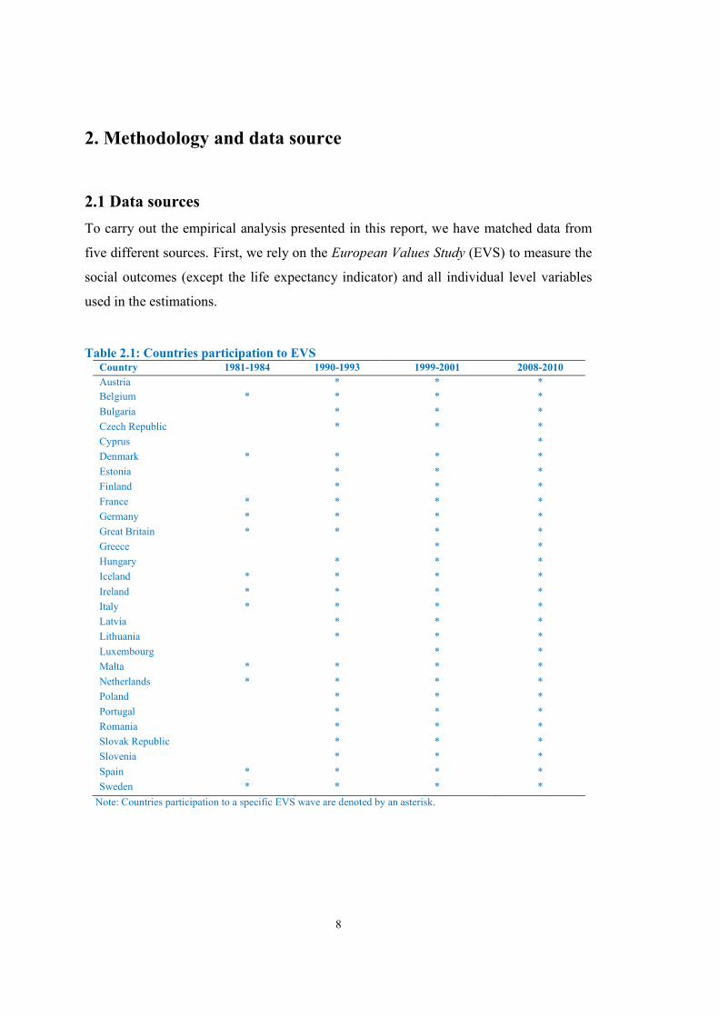
five different sources. First, we rely on the European Values Study (EVS) to measure the

social outcomes (except the life expectancy indicator) and all individual level variables

used in the estimations.

Table 2.1: Countries participation to EVS

Country 1981-1984 1990-1993 1999-2001 2008-2010

Austria * * *

Belgium * * * *

Bulgaria * * *

Czech Republic * * *

Cyprus *

Denmark * * * *

Estonia * * *

Finland * * *

France * * * *

Germany * * * *

Great Britain * * * *

Greece * *

Hungary * * *

Iceland * * * *

Ireland * * * *

Italy * * * *

Latvia * * *

Lithuania * * *

Luxembourg * *

Malta * * * *

Netherlands * * * *

Poland * * *

Portugal * * *

Romania * * *

Slovak Republic * * *

Slovenia * * *

Spain * * * *

Sweden * * * *

Note: Countries participation to a specific EVS wave are denoted by an asterisk.

9

The EVS was first launched in 1981, with the field work taking place over the period

1981-1983. Three additional waves followed, respectively in 1990, 1999 and 2008. For

these three waves, the field work was implemented respectively over the period 1990-

1993, 1999-2001 and 2008-2010. In Table 2.1, we report the EU countries participating

to each wave of the EVS. Eleven European countries participated to the first wave while

24 and 26 were part of respectively the second and third waves. Finally, all EU countries

are included in the last wave of the EVS. The EVS is a large scale, cross country and

repeated survey that provides information on the socioeconomic characteristics, ideas,

beliefs, preferences, attitudes, values and opinions of citizens of the persons interviewed.

The average country sample size is approximately 1500. In each country the sample is

representative of the adult population of 18 years and older who are resident within

private households, regardless of nationality and citizenship or language.5

Second, we employ the World Development Indicators (WDI) and the World Economic

Outlook Database (WEO) to gather country-specific information. The WDI database

includes more than 1,000 indicators for 216 economies, with long time series going back

to 1960 while the WEO is focused on macroeconomic data series with data available

since 1980 for 180 countries. 6 When an indicator used in the empirical analysis is

available in both datasets, we have selected the one from the WEO as this database

contains less missing values than the WDI. The 27 EU countries are covered by both

datasets, though with some missing data. Note that one indicator used in the empirical

analysis has been also taken from OECD Health Data (OECD, 2012).7

Finally, our measure of income disparity - the GINI coefficient - is taken from the World

Income Inequality Database (WIID) provided by the United Nations University – World

Institute for Development Economics Research. The updated data of the Deininger and

Squire (1996) from World Bank, the unit record data of the Luxembourg Income Study,

5 In Finland the sample is representative of the 18-74 years old population. See http://www.europeanvaluesstudy.eu/ for detailed information.

6 See http://data.worldbank.org/data-catalog/world-development-indicators and http://www.imf.org/external/pubs/ft/weo/2013/01/weodata/index.aspx for additional information.

7 See http://www.oecd.org/health/health-systems/oecdhealthdata2012.htm for additional information.

10

the Transmonee data by UNICEF/ICDC, Central Statistical Offices and research studies

are the main sources of the WIID. The WIID database, which collects information on

income inequality for developed, developing and transition countries, currently offers the

widest time series data coverage at the country level. In the empirical analysis, we rely on

the WIID data for measuring the GINI coefficient from the second half of the seventies

until 1998 while for the recent period we have used data from the European Statistical

Office, EUROSTAT.

2.2 Income inequality

2.2.1 Measurement issues

The WIID dataset reports two measures of the Gini coefficient. The first measure is

calculated using methods developed by Shorrocks and Wan (2008) and consists in

derivating the Gini coefficient using data on income deciles while the second measure is

the one originally reported by the source. The high correlation of 0.99 between the two

GINI coefficients suggests that both measures are substitutable. In the present analysis

we rely on the first measure since it has a better coverage both in terms of countries and

time periods.

The WIID data also reports several versions of the Gini index for the same country-year

pair, depending on the coverage of the surveys underlying the observations, the income

reference unit, the equivalence scale, or the income definition employed. More than 90%

of the surveys used for computing the Gini coefficient use samples of the whole

population while the 10% remaining are based on sub samples of the population (e.g.

workers). The reference unit is either the household (85% of cases) or the individual (15%

of cases). While the population coverage of the surveys and the reference unit do not

seem to pose particular problems, the income concept and the equivalence scale, on the

other hand, have a substantial impact on the Gini measure. In particular, the Gini index

varies according to the following income definitions: disposable income, monetary

disposable income, gross income, monetary gross income, net and gross earnings,

11

consumption and expenditure.8 In addition, when the reference unit is the household, the

income measure can be adjusted or not adjusted (i.e. not equivalised) to take into account

the difference in relative need of households of varying sizes. When adjusted, the

following equivalence scales can be used: the household size, the square root of the

household size, the OECD scale, the OECD-modified scale and for some countries a

specific national scale is applied (e.g. the UK uses the HBAI scale produced by the

Department for Work and Pensions). Unfortunately it is not possible to use a general

routine to sort the data, since the presence of missing values prevents us from choosing

an income definition (or equivalence scale), which would provide us with comparable

figures between and/or within country.

In order to have one data entry for every country-year observation, we had to select one

observation for those cases of multiple entries. We have applied a “pragmatic” algorithm,

which works as follows: we first select observations computed on disposable income; if

this information is not available we thus choose Gini coefficients based on either

monetary disposable income or gross income, otherwise we takes the Gini measures

calculated on earnings. As a result, we end up with a sample wherein 83% of the

observations are computed by using disposable income, 5% gross income, 2% monetary

disposable income, 6% gross earning and 4 % by using different income definitions. As

for the equivalence scale, the method aims, as far as possible, at selecting country

observations that make use of the same equivalence scale for the computation of the Gini

over the different periods.

All data on income inequality for the post-1996 taken from EUROSTAT are equivalised

using the OECD-modified scale. This implies that the 2 data points per country

corresponding to the two EVS waves having taken place after 1996, are based on the

same equivalence scale. In the previous period (i.e. the first two income inequality

measures linked to the first 2 EVS waves), data are less consistent: 35 % of the GINI

measures are equivalised by dividing the household income by the number of

household’s member, 40% of the observations come with no adjustment and 25% use a

8 For more detailed information about the income concept, see UNU-WIDER (2013).

12

national scale. The two income inequality measures per country corresponding to the two

EVS waves having taken place before 1993 have been selected in such a way as to

maximize the likelihood for a given country to have income inequality data based on the

same equivalence scale over these 2 periods. We are however aware that using inequality

values, which have been calculated by using different equivalence scales, might render

country comparisons problematic. However, as suggested by the sensitivity analysis

reported in Burniaux et al. (1998), while the level and, in particular, the composition of

income inequality are affected by the use of different equivalence scales, trends over time

and rankings across countries are much less affected. Furthermore, we have included in

the empirical analysis ����� dummies in order to specifically control for shifts in

equivalence scales and income. In this way, we should purge the Gini coefficients of the

variation created by these changes in its measurements.

2.3 Descriptive analysis

Before embarking on the analysis of the impact of income inequality on the three social

outcomes, i.e. health, social capital and happiness, we present some descriptive analysis

of our measure of income inequality, i.e. the Gini coefficient. In particular, we will assess

the variability of the Gini along two dimensions: (1) over the EU member states and (2)

over time.

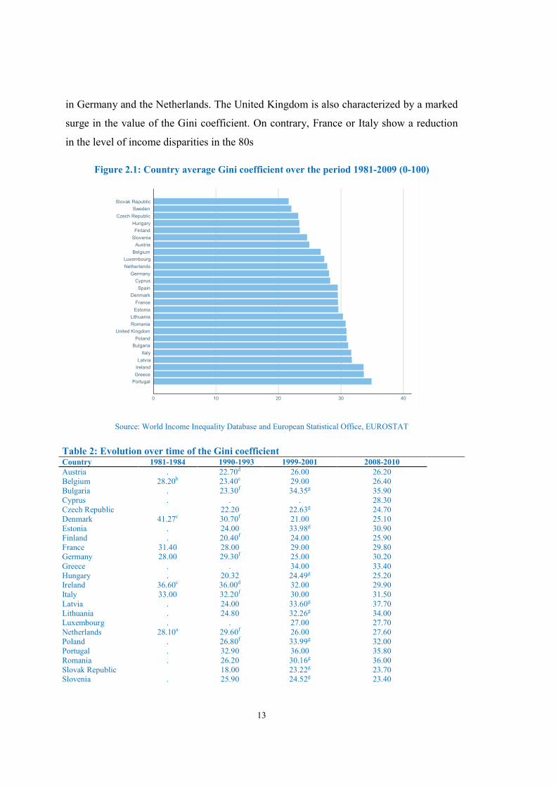
Figure 2.1 displays the country average Gini coefficient for 26 European member states

over the period 1981-2009. There exists a substantial variation across countries, with

Slovak Republic exhibiting the lowest levels of income inequality and Portugal

displaying the highest levels. Nordic countries as Sweden and Finland, which have

traditionally a more generous welfare system, hold the top positions, i.e. they are more

equal, with an average value of the Gini equal respectively to 22 and 23. Mediterranean

countries along with some Eastern countries rank very lowly, with Gini values ranging

between 30 and 35.

Table 2 depicts the evolution of the Gini coefficient over the 4 periods covered by the

EVS. In the first two periods covered by the EVS we observe a rise in income inequality

13

in Germany and the Netherlands. The United Kingdom is also characterized by a marked

surge in the value of the Gini coefficient. On contrary, France or Italy show a reduction

in the level of income disparities in the 80s

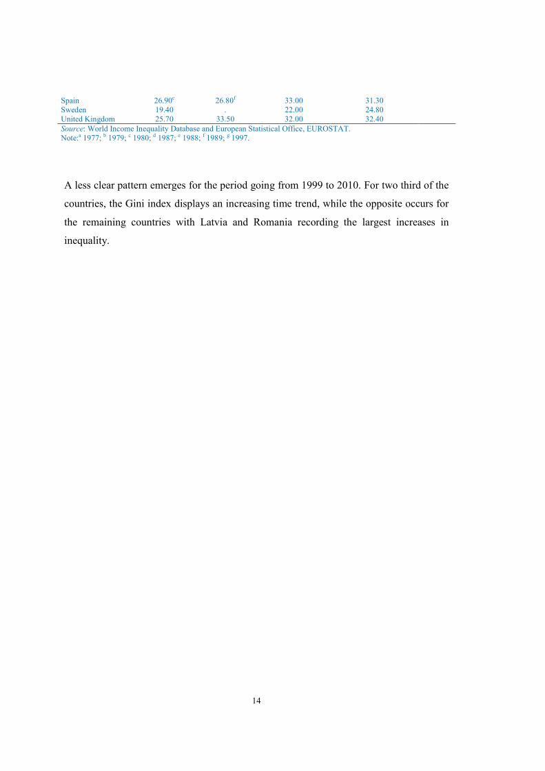
Figure 2.1: Country average Gini coefficient over the period 1981-2009 (0-100)

Source: World Income Inequality Database and European Statistical Office, EUROSTAT

Table 2: Evolution over time of the Gini coefficient Country 1981-1984 1990-1993 1999-2001 2008-2010 Austria . 22.70d 26.00 26.20 Belgium 28.20b 23.40e 29.00 26.40 Bulgaria . 23.30f 34.35g 35.90 Cyprus . . . 28.30 Czech Republic 22.20 22.63g 24.70 Denmark 41.27c 30.70f 21.00 25.10 Estonia . 24.00 33.98g 30.90 Finland . 20.40f 24.00 25.90 France 31.40 28.00 29.00 29.80 Germany 28.00 29.30f 25.00 30.20 Greece . . 34.00 33.40 Hungary . 20.32 24.49g 25.20 Ireland 36.60c 36.00d 32.00 29.90 Italy 33.00 32.20f 30.00 31.50 Latvia . 24.00 33.60g 37.70 Lithuania . 24.80 32.26g 34.00 Luxembourg . . 27.00 27.70 Netherlands 28.10a 29.60f 26.00 27.60 Poland . 26.80f 33.99g 32.00 Portugal . 32.90 36.00 35.80 Romania . 26.20 30.16g 36.00 Slovak Republic 18.00 23.22g 23.70 Slovenia . 25.90 24.52g 23.40

0 10 20 30 40

Portugal

Greece

Ireland

Latvia

Italy

Bulgaria

Poland

United Kingdom

Romania

Lithuania

Estonia

France

Denmark

Spain

Cyprus

Germany

Netherlands

Luxembourg

Belgium

Austria

Slovenia

Finland

Hungary

Czech Republic

Sweden

Slovak Republic

14

Spain 26.90c 26.80f 33.00 31.30 Sweden 19.40 . 22.00 24.80 United Kingdom 25.70 33.50 32.00 32.40 Source: World Income Inequality Database and European Statistical Office, EUROSTAT. Note:a 1977; b 1979; c 1980; d 1987; e 1988; f 1989; g 1997.

A less clear pattern emerges for the period going from 1999 to 2010. For two third of the

countries, the Gini index displays an increasing time trend, while the opposite occurs for

the remaining countries with Latvia and Romania recording the largest increases in

inequality.

15

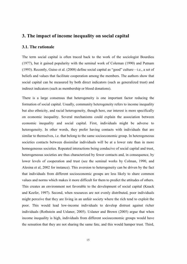
3. The impact of income inequality on social capital

3.1. The rationale

The term social capital is often traced back to the work of the sociologist Bourdieu

(1977), but it gained popularity with the seminal work of Coleman (1990) and Putnam

(1993). Recently, Guiso et al. (2008) define social capital as “good” culture—i.e., a set of

beliefs and values that facilitate cooperation among the members. The authors show that

social capital can be measured by both direct indicators (such as generalized trust) and

indirect indicators (such as membership or blood donations).

There is a large consensus that heterogeneity is one important factor reducing the

formation of social capital. Usually, community heterogeneity refers to income inequality

but also ethnicity, and racial heterogeneity, though here, our interest is more specifically

on economic inequality. Several mechanisms could explain the association between

economic inequality and social capital. First, individuals might be adverse to

heterogeneity. In other words, they prefer having contacts with individuals that are

similar to themselves, i.e. that belong to the same socioeconomic group. In heterogeneous

societies contacts between dissimilar individuals will be at a lower rate than in more

homogeneous societies. Repeated interactions being conducive of social capital and trust,

heterogeneous societies are thus characterized by fewer contacts and, in consequence, by

lower levels of cooperation and trust (see the seminal works by Colman, 1990, and

Alesina et al, 2002 for instance). This aversion to heterogeneity can be driven by the fact

that individuals from different socioeconomic groups are less likely to share common

values and norms which makes it more difficult for them to predict the attitudes of others.

This creates an environment not favorable to the development of social capital (Knack

and Keefer, 1997). Second, when resources are not evenly distributed, poor individuals

might perceive that they are living in an unfair society where the rich tend to exploit the

poor. This would lead low-income individuals to develop distrust against richer

individuals (Rothstein and Uslaner, 2005). Uslaner and Brown (2005) argue that when

income inequality is high, individuals from different socioeconomic groups would have

the sensation that they are not sharing the same fate, and this would hamper trust. Third,

16

inequality should relate to the level of optimism. A higher level of inequality is likely to

reduce the level of optimism for the future and thereby trust (Uslaner and Brown, 2005,

Rothstein and Uslaner, 2005).

3.2. Existing empirical evidence

Empirical studies on the relationship between heterogeneity and the level of social capital

are of three types. Cross-country papers explore either the association at the aggregated

level between income inequality and social capital or combine individual-level data on

social capital with country-level information on economic inequality. Studies on single

countries pool information on income inequality at the subnational level with individual

level information on social capital.

3.2.1 Cross-country studies

Most of the cross-country studies conclude that when income inequality is high, social

capital tends to be stunted (Knack and Keefer, 1997, Leigh, 2006a, Fisher and Torgler,

2006, Berggren and Jordhal, 2007, Bjornskov, 2006).

Based on aggregated country-level data drawn from the World Values Surveys, cross-

country estimates reported in Knack and Keefer (1997) show that income inequality is

negatively and significantly related to trust and civic cooperation. The empirical analysis

is based on 29 market countries, and several country-level controls are included in the

estimates.

Contrary to the studies mentioned above, Leigh (2006a) explores the relationship

between social capital and income inequality by combining individual data drawn from

the World Values Surveys in 59 countries with country measure of income dispersion.

The author finds that both income inequality and ethnic heterogeneity are negatively

associated with trust but that the effect of the former dominates the latter’s one. The

results hold even after taking into account the reciprocal relationship between income

17

inequality and social capital. 9 Using also the World Value Surveys, cross-country

estimates in Berggren and Jordhal (2006) confirm these findings. Fisher and Torgler

(2006) also working with individual data on trust for 25 countries observe that trust is

positively associated with a person's relative income position as measured by the

difference between a respondent’s income and the national (or regional) income.

While all the papers mentioned above find a strong negative association between social

capital and economic inequality, Steijn and Lancee (2011), on the contrary, conclude that

income inequality and perceived inequality do not correlate with trust once country

wealth is controlled for. Additionally, Lancee and Van de Werfhorst (2011) examine the

effect of income inequality in EU countries on various forms of social capital capturing

social, civic and cultural participation. The empirical work is based on the 2006 EU-

SILC survey and demonstrates that though civic participation is significantly associated

with economic inequality social and cultural participation are not.

3.2.2 Single-country studies

Research based on a single country generally relies on a multilevel approach. Social

capital is measured at the individual level and explained by both individual

socioeconomic characteristics (age, educational attainment, income, gender, etc) and the

social context in which the respondents are living (in particular, the level of community

heterogeneity). This social context is defined at the municipal/neighborhood level

(Alesina and La Ferrara, 2000, 2002, Leigh, 2006a, Costas and Kahn, 2003, Coffe and

Geys, 2006, Gustavsson and Jordhal, 2008).

A significant literature has documented the negative effect of community heterogeneity

on social capital across metropolitan areas in the US. Alesina and La Ferrara (2000 and

2002) use cross-sectional data from the US General Social Surveys over the period 1974-

1994 to examine the effect of community heterogeneity on membership and trust. After

9 To account for the reciprocal relationship between income inequality and social capital, the author

instruments income inequality with the ratio of the size of the cohort aged between 40 and 59 to the population aged 15 to 69.

18

having controlled for individual and some community characteristics as well as for year

and state-fixed effects, the authors find that respondents living in more racially

fragmented and income unequal communities report lower levels of social capital.

However, the effect of racial heterogeneity is even stronger and income inequality has no

longer a significant effect on trust when this variable is added to the empirical model.

Costas and Kahn (2003) also observe a negative impact of community heterogeneity on

various measures of social capital (volunteering and membership in organizations), once

they control for individual characteristics as well as for time and regional dummies.

However, in contrast to Alesina and La Ferrara (2000 and 2002) their results suggest that

the crucial determinant of volunteering and membership in organizations is income

inequality.10,11 Tesei (2011), using the decomposability of the Theil index, shows that

what really matters is income inequality between racial groups. While racial

fragmentation and economic inequality are both significantly associated with trust and

group participation, these effects become insignificant when income inequality between

racial groups is accounted for.

Solid empirical evidence on the relationship between social capital and income inequality

outside the US are quite limited. Leigh (2006b) analyzes the determinants of localized

trust (trusting those living in the same neighborhoods) and generalized trust (trusting

those who live in the same country) in Australia using individual data over the period

1997-1998 combined with information on the neighborhood in which the respondents are

living. Results suggest that there is not an apparent relationship between inequality and

trust and this finding remains identical when the author accounts for the possible

“endogeneity” of income inequality. Coffe and Geys (2006) explore the effect of income

inequality on the municipality level of social capital in 307 Flemish municipalities in

2000. The authors rely on three indicators measuring social capital in a broad sense:

associational life, electoral participation and crime rate that are combined into a single

index using a principal component analysis. After having controlled for several

10

Costas and Kahn (2003) also find that the increase in the participation of women on the labour market is the main responsible for the decline in social capital produced inside home (entertaining friends and relatives). 11

Note that when the authors correct for the endogeneity of income inequality in the volunteering equation, the coefficients associated with income inequality becomes insignificant.

19

socioeconomic characteristics of the municipality, the authors do not observe any effect

of income inequality on social capital. On contrary, ethnic heterogeneity has a depressing

effect on social capital.

Finally, Gustavsson and Jordhal (2008) combine Swedish individual-level panel data

(1994-1998) on trust with county level measures of inequality. The results suggest that

different measures of income inequality lead to different conclusions. The Gini

coefficient is weakly related to trust while the ratio of the 50th over the 10th percentile

income displays a negative and significant association with trust suggesting that

differences in the bottom half of the income distribution matter most for explaining trust.

Compared to Alesina and La Ferrara (2000, 2002), Leigh (2006b) or Costas and Kahn

(2003), the panel data employed in this study allows for controlling for time-invariant

individual and county characteristics in addition to the conventional time-varying

individual covariates, implying that the estimated association between social capital and

income inequality is very likely to be a causal one.

In conclusion, macro studies usually conclude that income inequality depresses social

capital while micro studies seem to produce more contrasted results (see Table 4.1 for an

overview of the studies). However macro studies are sometimes problematic when it

comes to making causal statements. Indeed, this body of literature is mainly grounded on

cross-sectional data (i.e., one point per country), meaning that it is not possible to control

for all potential time-invariant country specific-effects (and thus to look at the effect,

within a country, of income inequality changes on social capital formation). Single

country based studies have the main advantage of keeping constant country-specific

determinants of trust which are susceptible to bias cross-country estimates if they are not

controlled for.12 Micro studies produce more contrasted results than macro analyses. In

the USA, there seems to be a robust negative association between community

heterogeneity and social capital. Findings for other countries are less conclusive.

12

Furthermore, while income inequality measures used for cross-comparisons are subject to measurement comparability issues, this is less the case when one relies on income inequality measures of different geographical units within a given country.

20

While the empirical analysis presented in this chapter examines the relationship between

income inequality and social capital in a cross-country context, contrary to the

aforementioned macro studies, a longer time period (1981-2008) is covered and the time-

invariant country heterogeneity is accounted for.

21

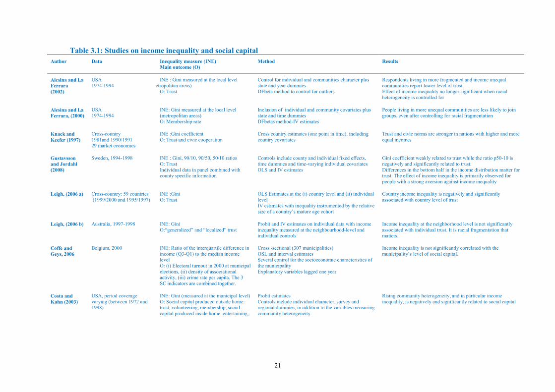
Table 3.1: Studies on income inequality and social capital

Author Data Inequality measure (INE) Main outcome (O)

Method Results

Alesina and La Ferrara (2002)

USA 1974-1994

INE : Gini measured at the local level (metropolitan areas)

O: Trust

Control for individual and communities character plus state and year dummies DFbeta method to control for outliers

Respondents living in more fragmented and income unequal communities report lower level of trust Effect of income inequality no longer significant when racial heterogeneity is controlled for

Alesina and La Ferrara, (2000)

USA 1974-1994

INE: Gini measured at the local level (metropolitan areas) O: Membership rate

Inclusion of individual and community covariates plus state and time dummies DFbetas method-IV estimates

People living in more unequal communities are less likely to join groups, even after controlling for racial fragmentation

Knack and Keefer (1997)

Cross-country 1981and 1990/1991 29 market economies

INE :Gini coefficient O: Trust and civic cooperation

Cross country estimates (one point in time), including country covariates

Trust and civic norms are stronger in nations with higher and more equal incomes

Gustavsson and Jordahl (2008)

Sweden, 1994-1998

INE : Gini, 90/10, 90/50, 50/10 ratios O: Trust Individual data in panel combined with county specific information

Controls include county and individual fixed effects, time dummies and time-varying individual covariates OLS and IV estimates

Gini coefficient weakly related to trust while the ratio p50-10 is negatively and significantly related to trust. Differences in the bottom half in the income distribution matter for trust. The effect of income inequality is primarily observed for people with a strong aversion against income inequality

Leigh, (2006 a) Cross-country: 59 countries (1999/2000 and 1995/1997)

INE :Gini O: Trust

OLS Estimates at the (i) country level and (ii) individual level IV estimates with inequality instrumented by the relative size of a country’s mature age cohort

Country income inequality is negatively and significantly associated with country level of trust

Leigh, (2006 b) Australia, 1997-1998 INE: Gini O:“generalized” and “localized” trust

Probit and IV estimates on individual data with income inequality measured at the neighbourhood-level and individual controls

Income inequality at the neighborhood level is not significantly associated with individual trust. It is racial fragmentation that matters.

Coffe and Geys, 2006

Belgium, 2000 INE: Ratio of the interquartile difference in income (Q3-Q1) to the median income level O: (i) Electoral turnout in 2000 at municipal elections, (ii) density of associational activity, (iii) crime rate per capita. The 3 SC indicators are combined together.

Cross -sectional (307 municipalities) OSL and interval estimates Several control for the socioeconomic characteristics of the municipality Explanatory variables lagged one year

Income inequality is not significantly correlated with the municipality’s level of social capital.

Costa and Kahn (2003)

USA, period coverage varying (between 1972 and 1998)

INE: Gini (measured at the municipal level) O: Social capital produced outside home: trust, volunteering, membership, social capital produced inside home: entertaining,

Probit estimates Controls include individual character, survey and regional dummies, in addition to the variables measuring community heterogeneity.

Rising community heterogeneity, and in particular income inequality, is negatively and significantly related to social capital

22

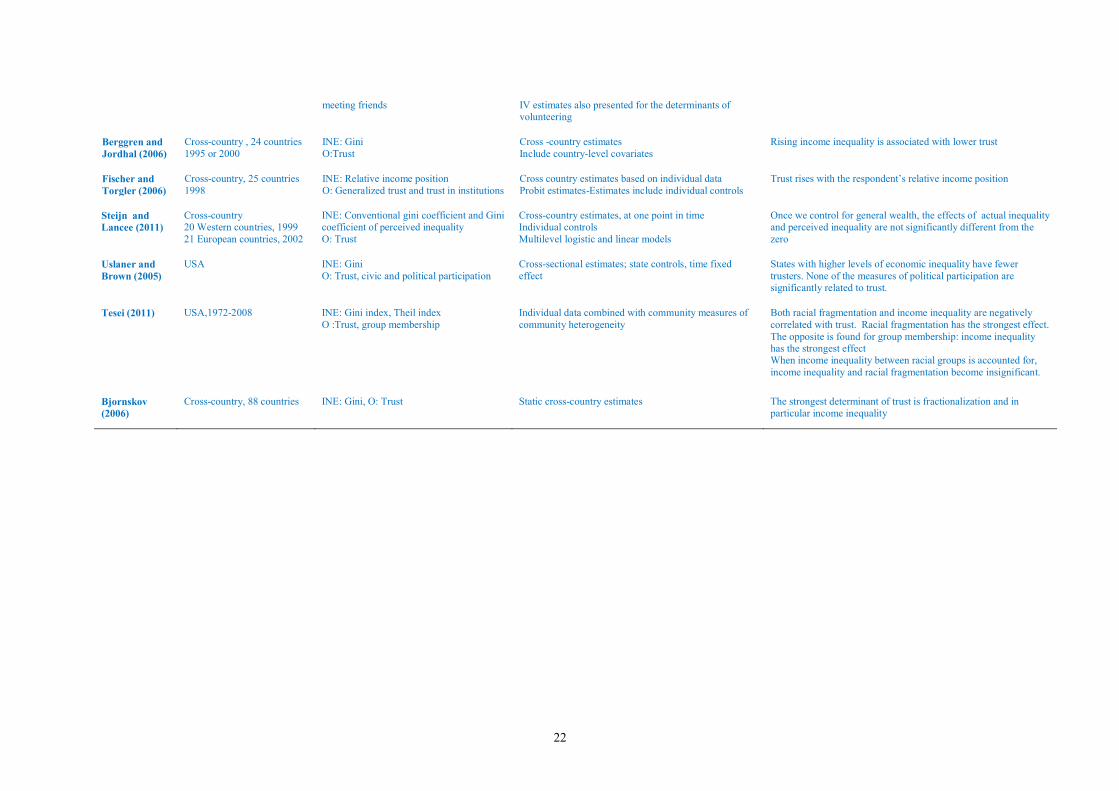
meeting friends IV estimates also presented for the determinants of volunteering

Berggren and Jordhal (2006)

Cross-country , 24 countries 1995 or 2000

INE: Gini O:Trust

Cross -country estimates Include country-level covariates

Rising income inequality is associated with lower trust

Fischer and Torgler (2006)

Cross-country, 25 countries 1998

INE: Relative income position O: Generalized trust and trust in institutions

Cross country estimates based on individual data Probit estimates-Estimates include individual controls

Trust rises with the respondent’s relative income position

Steijn and Lancee (2011)

Cross-country 20 Western countries, 1999 21 European countries, 2002

INE: Conventional gini coefficient and Gini coefficient of perceived inequality O: Trust

Cross-country estimates, at one point in time Individual controls Multilevel logistic and linear models

Once we control for general wealth, the effects of actual inequality and perceived inequality are not significantly different from the zero

Uslaner and Brown (2005)

USA INE: Gini O: Trust, civic and political participation

Cross-sectional estimates; state controls, time fixed effect

States with higher levels of economic inequality have fewer trusters. None of the measures of political participation are significantly related to trust.

Tesei (2011) USA,1972-2008 INE: Gini index, Theil index O :Trust, group membership

Individual data combined with community measures of community heterogeneity

Both racial fragmentation and income inequality are negatively correlated with trust. Racial fragmentation has the strongest effect. The opposite is found for group membership: income inequality has the strongest effect When income inequality between racial groups is accounted for, income inequality and racial fragmentation become insignificant.

Bjornskov (2006)

Cross-country, 88 countries INE: Gini, O: Trust Static cross-country estimates The strongest determinant of trust is fractionalization and in particular income inequality

23

3.3. Empirical analysis

3.3.1 Social capital variables

We operationalize social capital with two indicators. The first social capital indicator captures

the level of generalized trust reported by each respondent of the EVS. Trust constitutes a proxy

for cognitive social capital and its use is motivated by several academic papers. In particular,

Guiso et al. (2008 and 2010) consider that direct indicators, such as generalized trust, are

adequate if social capital is considered as an individual belief about the willingness of other

members of the community to cooperate.13

In the European Value Study, respondents are asked “Generally speaking would you say that

“most people can be trusted” or that “you can’t be too careful in dealing with people”. The

yes/no nature of the response enable us to construct a variable trust which is equal to one if the

respondent reports that “most people can be trusted” and equal to 0 otherwise.

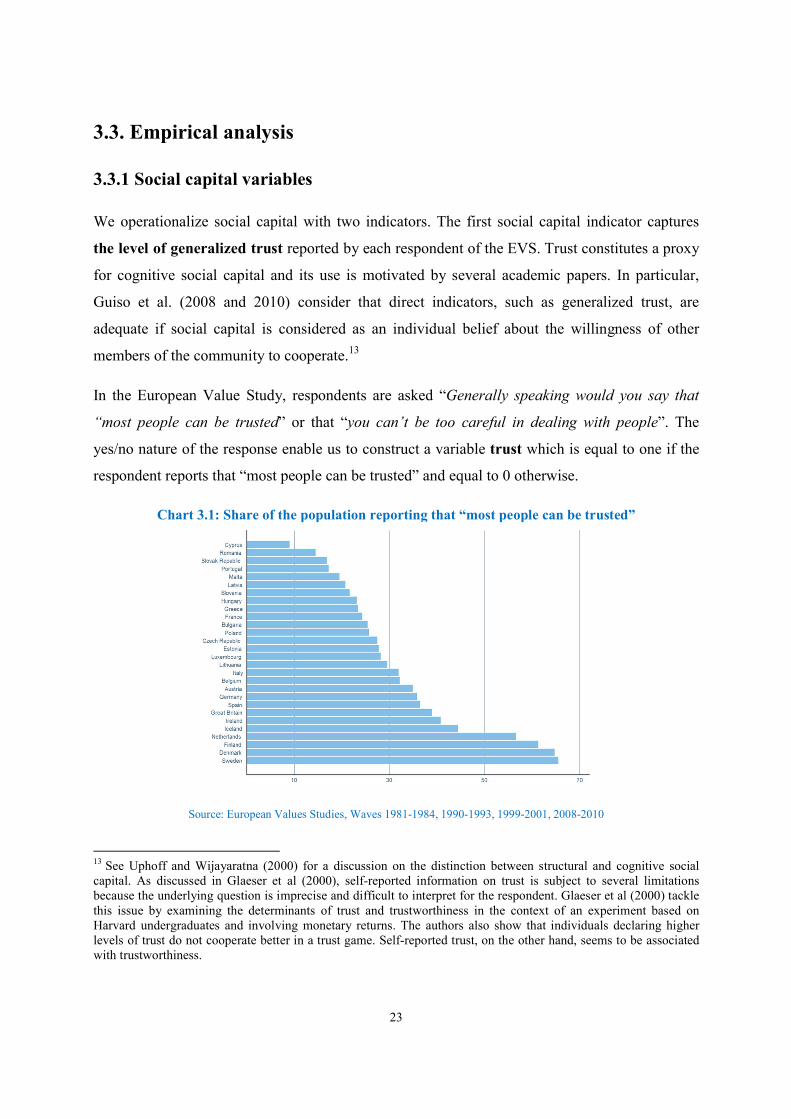
Chart 3.1: Share of the population reporting that “most people can be trusted”

Source: European Values Studies, Waves 1981-1984, 1990-1993, 1999-2001, 2008-2010

13 See Uphoff and Wijayaratna (2000) for a discussion on the distinction between structural and cognitive social capital. As discussed in Glaeser et al (2000), self-reported information on trust is subject to several limitations because the underlying question is imprecise and difficult to interpret for the respondent. Glaeser et al (2000) tackle this issue by examining the determinants of trust and trustworthiness in the context of an experiment based on Harvard undergraduates and involving monetary returns. The authors also show that individuals declaring higher levels of trust do not cooperate better in a trust game. Self-reported trust, on the other hand, seems to be associated with trustworthiness.

24

Chart 3.1 displays the country average value of the indicator. It is apparent that the level of trust

greatly varies across countries. In Nordic countries, such as Sweden, Denmark or Finland, more

than 60% of respondents are trustful while, on the opposite, in Cyprus, Romania, Slovak

Republic or Portugal, less than one respondent out of 5 reports that most people can be trusted.

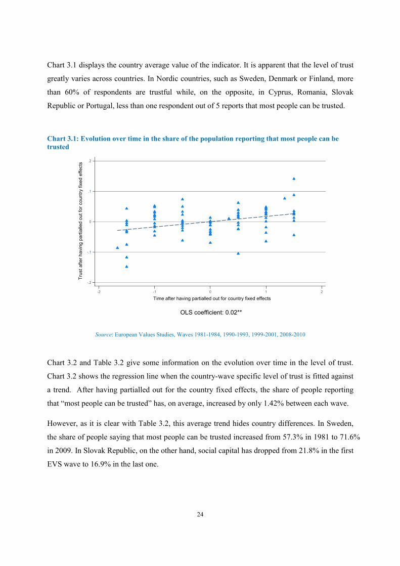
Chart 3.1: Evolution over time in the share of the population reporting that most people can be trusted

Source: European Values Studies, Waves 1981-1984, 1990-1993, 1999-2001, 2008-2010

Chart 3.2 and Table 3.2 give some information on the evolution over time in the level of trust.

Chart 3.2 shows the regression line when the country-wave specific level of trust is fitted against

a trend. After having partialled out for the country fixed effects, the share of people reporting

that “most people can be trusted” has, on average, increased by only 1.42% between each wave.

However, as it is clear with Table 3.2, this average trend hides country differences. In Sweden,

the share of people saying that most people can be trusted increased from 57.3% in 1981 to 71.6%

in 2009. In Slovak Republic, on the other hand, social capital has dropped from 21.8% in the first

EVS wave to 16.9% in the last one.

-.2

-.1

0

.1

.2

Tru

st a

fte

r h

avi

ng

pa

rtia

lled

ou

t fo

r co

un

try

fixe

d e

ffe

cts

-2 -1 0 1 2

Time after having partialled out for country fixed effects

OLS coefficient: 0.02**

25

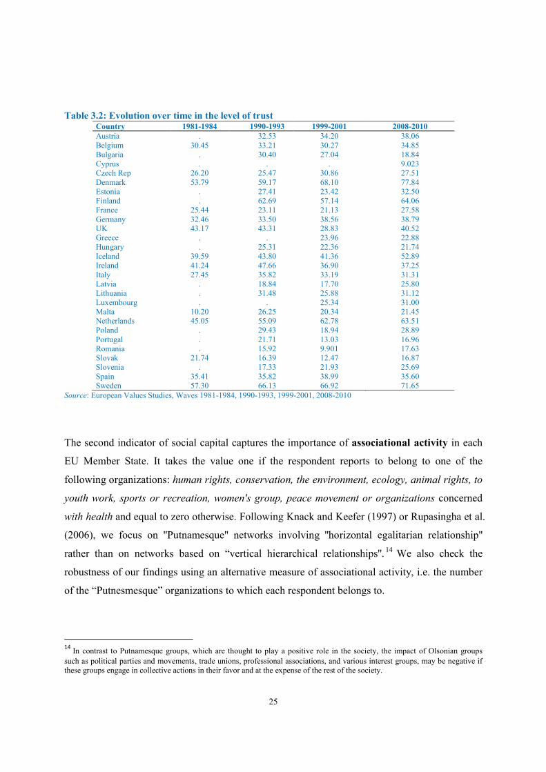
Table 3.2: Evolution over time in the level of trust Country 1981-1984 1990-1993 1999-2001 2008-2010 Austria . 32.53 34.20 38.06 Belgium 30.45 33.21 30.27 34.85 Bulgaria . 30.40 27.04 18.84 Cyprus . . . 9.023 Czech Rep 26.20 25.47 30.86 27.51 Denmark 53.79 59.17 68.10 77.84 Estonia . 27.41 23.42 32.50 Finland . 62.69 57.14 64.06 France 25.44 23.11 21.13 27.58 Germany 32.46 33.50 38.56 38.79 UK 43.17 43.31 28.83 40.52 Greece . . 23.96 22.88 Hungary . 25.31 22.36 21.74 Iceland 39.59 43.80 41.36 52.89 Ireland 41.24 47.66 36.90 37.25 Italy 27.45 35.82 33.19 31.31 Latvia . 18.84 17.70 25.80 Lithuania . 31.48 25.88 31.12 Luxembourg . . 25.34 31.00 Malta 10.20 26.25 20.34 21.45 Netherlands 45.05 55.09 62.78 63.51 Poland . 29.43 18.94 28.89 Portugal . 21.71 13.03 16.96 Romania . 15.92 9.901 17.63 Slovak 21.74 16.39 12.47 16.87 Slovenia . 17.33 21.93 25.69 Spain 35.41 35.82 38.99 35.60 Sweden 57.30 66.13 66.92 71.65

Source: European Values Studies, Waves 1981-1984, 1990-1993, 1999-2001, 2008-2010

The second indicator of social capital captures the importance of associational activity in each

EU Member State. It takes the value one if the respondent reports to belong to one of the

following organizations: human rights, conservation, the environment, ecology, animal rights, to

youth work, sports or recreation, women's group, peace movement or organizations concerned

with health and equal to zero otherwise. Following Knack and Keefer (1997) or Rupasingha et al.

(2006), we focus on ''Putnamesque'' networks involving ''horizontal egalitarian relationship''

rather than on networks based on “vertical hierarchical relationships''. 14 We also check the

robustness of our findings using an alternative measure of associational activity, i.e. the number

of the “Putnesmesque” organizations to which each respondent belongs to.

14 In contrast to Putnamesque groups, which are thought to play a positive role in the society, the impact of Olsonian groups

such as political parties and movements, trade unions, professional associations, and various interest groups, may be negative if these groups engage in collective actions in their favor and at the expense of the rest of the society.

26

Though being member of an organization might be desirable per se, it does not convey

automatically the benefits expected from social capital as the actual advantages depend on the

type of relationship within the organization. The data we are using do not allow making such a

distinction.

However, participation in associational activities has been largely used in the literature either in

this form or in a closely related formulation and is intended to measure “structural'' social capital,

i.e. social networks that entails mutual beneficial actions. Participation in specific organizations

reduces the “social distance” between individuals and should promote trust and cooperation

(Glaeser et al, 2000). Furthermore, in societies with high income inequality, individuals

belonging to the lower end of the income distribution are expected to report lower participation

for income or distress-related feeling reasons (Lancee and Van de Werfhorst, 2011).

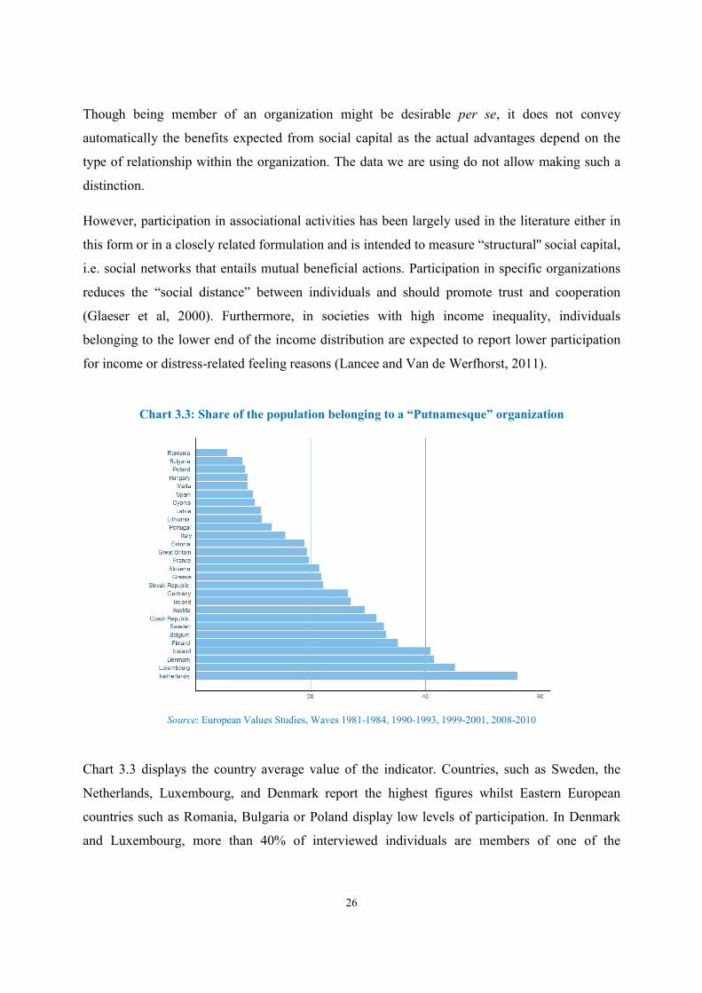
Chart 3.3: Share of the population belonging to a “Putnamesque” organization

Source: European Values Studies, Waves 1981-1984, 1990-1993, 1999-2001, 2008-2010

Chart 3.3 displays the country average value of the indicator. Countries, such as Sweden, the

Netherlands, Luxembourg, and Denmark report the highest figures whilst Eastern European

countries such as Romania, Bulgaria or Poland display low levels of participation. In Denmark

and Luxembourg, more than 40% of interviewed individuals are members of one of the

27

organizations described above. Conversely, in Poland and Romania this indicator scores below

10%.

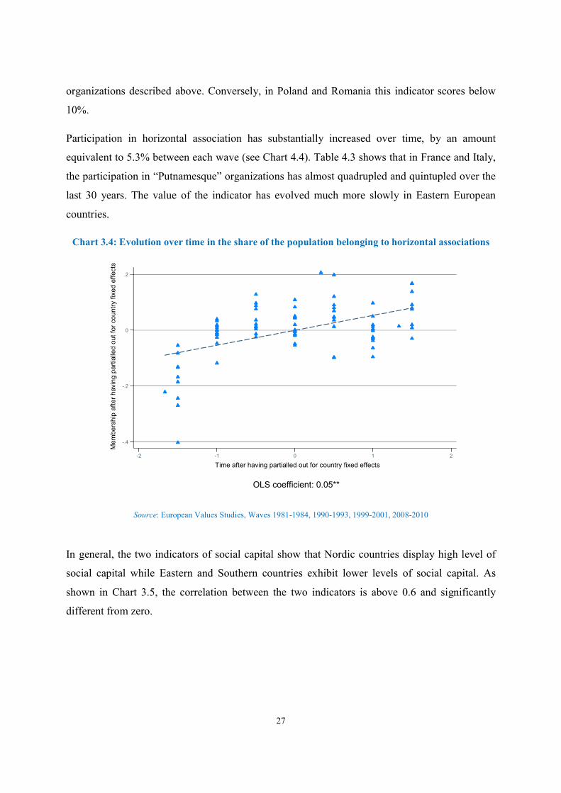
Participation in horizontal association has substantially increased over time, by an amount

equivalent to 5.3% between each wave (see Chart 4.4). Table 4.3 shows that in France and Italy,

the participation in “Putnamesque” organizations has almost quadrupled and quintupled over the

last 30 years. The value of the indicator has evolved much more slowly in Eastern European

countries.

Chart 3.4: Evolution over time in the share of the population belonging to horizontal associations

Source: European Values Studies, Waves 1981-1984, 1990-1993, 1999-2001, 2008-2010

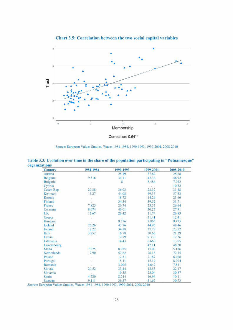
In general, the two indicators of social capital show that Nordic countries display high level of

social capital while Eastern and Southern countries exhibit lower levels of social capital. As

shown in Chart 3.5, the correlation between the two indicators is above 0.6 and significantly

different from zero.

-.4

-.2

0

.2

Mem

bers

hip

aft

er

havi

ng p

art

ialle

d o

ut fo

r co

untr

y f

ixed e

ffects

-2 -1 0 1 2

Time after having partialled out for country fixed effects

OLS coefficient: 0.05**

28

Chart 3.5: Correlation between the two social capital variables

Source: European Values Studies, Waves 1981-1984, 1990-1993, 1999-2001, 2008-2010

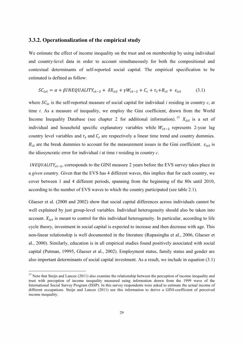
Table 3.3: Evolution over time in the share of the population participating in “Putnamesque” organizations

Country 1981-1984 1990-1993 1999-2001 2008-2010 Austria . 25.19 37.62 25.68 Belgium 9.316 34.11 42.36 46.92 Bulgaria . 8 8.486 7.932 Cyprus . . . 10.32 Czech Rep 29.38 36.93 28.12 31.48 Denmark 15.27 44.08 49.35 57.33 Estonia . 18.72 14.29 23.66 Finland . 34.34 39.52 31.71 France 7.825 20.74 23.55 26.64 Germany 8.074 40.01 30.27 27.91 UK 12.67 26.42 11.74 26.83 Greece . . 31.41 12.41 Hungary . 9.756 7.865 9.475 Iceland 26.26 43.76 44.95 48.46 Ireland 12.22 34.18 37.79 23.52 Italy 3.852 16.78 20.66 21.29 Latvia . 12.79 9.330 12.26 Lithuania . 14.43 6.660 13.65 Luxembourg . . 42.11 48.20 Malta 7.075 8.955 15.02 5.186 Netherlands 17.90 57.62 76.18 72.35 Poland . 12.31 7.187 6.468 Portugal . 15.41 15.19 8.904 Romania . 3.905 4.642 7.831 Slovak 20.52 33.44 12.53 22.17 Slovenia . 10.55 23.04 30.87 Spain 4.720 8.244 16.96 10.11 Sweden 9.111 39.57 51.67 30.73

Source: European Values Studies, Waves 1981-1984, 1990-1993, 1999-2001, 2008-2010

0

.2

.4

.6

.8T

rust

0 .2 .4 .6 .8

Membership

Correlation: 0.64**

29

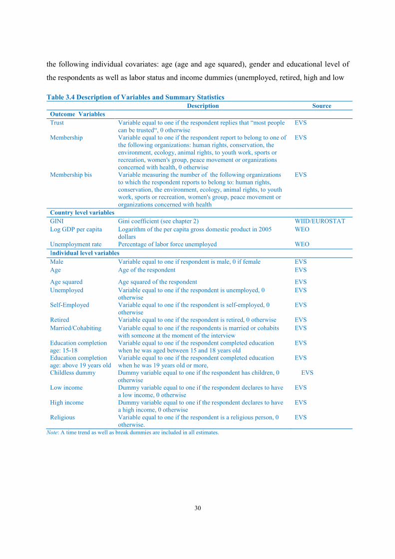
3.3.2. Operationalization of the empirical study

We estimate the effect of income inequality on the trust and on membership by using individual

and country-level data in order to account simultaneously for both the compositional and

contextual determinants of self-reported social capital. The empirical specification to be

estimated is defined as follow:

����� = � + ��������������� +����� + ������ + �� + ��+��� + ���� (3.1)

where ���� is the self-reported measure of social capital for individual i residing in country c, at

time t. As a measure of inequality, we employ the Gini coefficient, drawn from the World

Income Inequality Database (see chapter 2 for additional information). 15 ���� is a set of

individual and household specific explanatory variables while ����� represents 2-year lag

country level variables and ��and �� are respectively a linear time trend and country dummies.

��� are the break dummies to account for the measurement issues in the Gini coefficient. ���� is

the idiosyncratic error for individual i at time t residing in country c.

��������������, corresponds to the GINI measure 2 years before the EVS survey takes place in

a given country. Given that the EVS has 4 different waves, this implies that for each country, we

cover between 1 and 4 different periods, spanning from the beginning of the 80s until 2010,

according to the number of EVS waves to which the country participated (see table 2.1).

Glaeser et al. (2000 and 2002) show that social capital differences across individuals cannot be

well explained by just group-level variables. Individual heterogeneity should also be taken into

account. ���� is meant to control for this individual heterogeneity. In particular, according to life

cycle theory, investment in social capital is expected to increase and then decrease with age. This

non-linear relationship is well documented in the literature (Rupasingha et al., 2006, Glaeser et

al., 2000). Similarly, education is in all empirical studies found positively associated with social

capital (Putman, 19995, Glaeser et al., 2002). Employment status, family status and gender are

also important determinants of social capital investment. As a result, we include in equation (3.1)

15

Note that Steijn and Lancee (2011) also examine the relationship between the perception of income inequality and trust with perception of income inequality measured using information drawn from the 1999 wave of the International Social Survey Program (ISSP). In this survey respondents were asked to estimate the actual income of different occupations. Steijn and Lancee (2011) use this information to derive a GINI-coefficient of perceived income inequality.

30

the following individual covariates: age (age and age squared), gender and educational level of

the respondents as well as labor status and income dummies (unemployed, retired, high and low

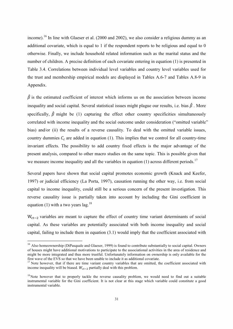
Table 3.4 Description of Variables and Summary Statistics Description Source

Outcome Variables

Trust Variable equal to one if the respondent replies that “most people can be trusted“, 0 otherwise

EVS

Membership Variable equal to one if the respondent report to belong to one of the following organizations: human rights, conservation, the environment, ecology, animal rights, to youth work, sports or recreation, women's group, peace movement or organizations concerned with health, 0 otherwise

EVS

Membership bis Variable measuring the number of the following organizations to which the respondent reports to belong to: human rights, conservation, the environment, ecology, animal rights, to youth work, sports or recreation, women's group, peace movement or organizations concerned with health

EVS

Country level variables

GINI Gini coefficient (see chapter 2) WIID/EUROSTAT

Log GDP per capita Logarithm of the per capita gross domestic product in 2005 dollars

WEO

Unemployment rate Percentage of labor force unemployed WEO

Individual level variables

Male Variable equal to one if respondent is male, 0 if female EVS

Age Age of the respondent EVS

Age squared Age squared of the respondent EVS

Unemployed Variable equal to one if the respondent is unemployed, 0 otherwise

EVS

Self-Employed Variable equal to one if the respondent is self-employed, 0 otherwise

EVS

Retired Variable equal to one if the respondent is retired, 0 otherwise EVS

Married/Cohabiting Variable equal to one if the respondents is married or cohabits with someone at the moment of the interview

EVS

Education completion age: 15-18

Variable equal to one if the respondent completed education when he was aged between 15 and 18 years old

EVS

Education completion age: above 19 years old

Variable equal to one if the respondent completed education when he was 19 years old or more,

EVS

Childless dummy Dummy variable equal to one if the respondent has children, 0 otherwise

EVS

Low income Dummy variable equal to one if the respondent declares to have a low income, 0 otherwise

EVS

High income Dummy variable equal to one if the respondent declares to have a high income, 0 otherwise

EVS

Religious Variable equal to one if the respondent is a religious person, 0 otherwise.

EVS

Note: A time trend as well as break dummies are included in all estimates.

31

income).16 In line with Glaeser et al. (2000 and 2002), we also consider a religious dummy as an

additional covariate, which is equal to 1 if the respondent reports to be religious and equal to 0

otherwise. Finally, we include household related information such as the marital status and the

number of children. A precise definition of each covariate entering in equation (1) is presented in

Table 3.4. Correlations between individual level variables and country level variables used for

the trust and membership empirical models are displayed in Tables A.6-7 and Tables A.8-9 in

Appendix.

��is the estimated coefficient of interest which informs us on the association between income

inequality and social capital. Several statistical issues might plague our results, i.e. bias ��. More

specifically, ��might be (1) capturing the effect other country specificities simultaneously

correlated with income inequality and the social outcome under consideration (“omitted variable”

bias) and/or (ii) the results of a reverse causality. To deal with the omitted variable issues,

country dummies ��are added in equation (1). This implies that we control for all country-time

invariant effects. The possibility to add country fixed effects is the major advantage of the

present analysis, compared to other macro studies on the same topic. This is possible given that

we measure income inequality and all the variables in equation (1) across different periods.17

Several papers have shown that social capital promotes economic growth (Knack and Keefer,

1997) or judicial efficiency (La Porta, 1997), causation running the other way, i.e. from social

capital to income inequality, could still be a serious concern of the present investigation. This

reverse causality issue is partially taken into account by including the Gini coefficient in

equation (1) with a two years lag.18

W���� variables are meant to capture the effect of country time variant determinants of social

capital. As these variables are potentially associated with both income inequality and social

capital, failing to include them in equation (3.1) would imply that the coefficient associated with

16 Also homeownership (DiPasquale and Glaeser, 1999) is found to contribute substantially to social capital. Owners of houses might have additional motivations to participate to the associational activities in the area of residence and might be more integrated and thus more trustful. Unfortunately information on ownership is only available for the first wave of the EVS so that we have been unable to include it as additional covariate. 17 Note however, that if there are time variant country variables that are omitted, the coefficient associated with income inequality will be biased. �����partially deal with this problem.

18 Note however that to properly tackle the reverse causality problem, we would need to find out a suitable instrumental variable for the Gini coefficient. It is not clear at this stage which variable could constitute a good instrumental variable.

32

income inequality would capture not only the effect of income inequality but also the influence

of those additional variables on social capital. We thus include the two following

macroeconomic covariates: the unemployment rate and the logarithm of GDP per capita, in 2005

US dollars at purchasing power parity. These figures are both drawn from the WEO dataset

provided by the IMF.

Note that ethnic, religious or linguistic heterogeneities have often been cited as factors of social

tensions (Putman, 1995, Leigh, 2006a, Rupasingha et al., 2006, Alesina and la Ferrara, 2000 and

2002) with detrimental effects on social capital accumulation, and trust in particular. Several

papers discuss the relative importance of income inequality versus ethnic heterogeneity on social

capital (Leigh, 2006a, Alesina and La Ferrara, 200 and 2002, Costas and Kahn, 2003), without

reaching a definite conclusion. Moreover, the most commonly used proxy for ethnic diversity,

the ethnic fractionalization index proposed by Alesina et al (2003), only covers one year per

country and as such is inadequate for the present analysis. However, we are still able to allow for

time-invariant ethnic heterogeneity thanks to the inclusion of the country fixed effects in

equation (3.1).

Because recent analyses demonstrate that the presence of pervasive serial correlation in country

level fixed effect models and the use of group-level variables may produce severely downward-

biased standard errors (Bertrand, Duflo, and Mullainathan 2001; Donald and Lang 2001), we

employ Huber-White standard errors clustered at the country level throughout the estimations.

These standard errors are robust to arbitrary forms of error correlation within a country. Since to

the authors’ knowledge most empirical papers have neglected this issue so far, therefore this

“correction” is one of the major advantages of the present analysis.

3.3.3 Econometric results

Table 3.5 presents the estimated coefficients of the model (3.1). Model of column 1 includes the

Gini coefficient, a linear trend as well as country and break dummies. Because of the country

fixed effects, the coefficient associated with income inequality is identified only through within

country variations. In column 2, we include individual level variables while in column 3, we also

33

control for the 2 time-varying macroeconomic variables. Linear models are used for estimating

equation (4.1) and the t-statistics reported in brackets are clustered at the country level.

Trust and income inequality

Results reported in the first column of Table 3.5 show that income inequality is not related to

trust when no individual and macroeconomics covariates are included in equation (3.1). However,

when we control for the individual characteristics, the coefficient associated with the Gini index

becomes significantly different from zero and the negative sign suggests that people are more

trustful in countries with low levels of income disparity. Adding country time-variant variables

(column 3) makes the estimate of the relationship between income inequality and trust even more

precise. This result is opposite to Stein and Lancee (2011). Indeed, the authors conclude that

income inequality is no longer related to trust when wealth differences across countries are taken

into account. However, Stein and Lancee (2011) do not include country fixed effects given that

their data are cross-sectional. We thus think that their findings are less robust than those

presented here.

The magnitude of the coefficient associated to the Gini coefficient doubles when we include time

country variables, moving from -0.004 in column 2 to -0.008 in column 3. Based on the latter, it

means that if the Gini coefficient in Romania drops to the Swedish level, i.e. from 36 to 25 (2008

levels), the average value of the trust indicator will increase in Romania by almost 54%19.

Analogously, if the value of the Gini coefficient decreases by one standard deviation (4.32), then

the average value of trust in the sample will rise by 10%.

Results reported in the last 4 columns of Table 3.5 suggest that the relationship between trust and

income inequality is robust to alternative specifications. In columns 4 and 5, we have estimated

equation (3.1) using different lag structures of the Gini coefficient. In particular, in columns 4

and 5, we assume that income inequality affects trust, with respectively no lag and one year lag.

In column 6, we use a three year moving average centered on year t-2 to smooth out some of the

noise associated with the construction of the Gini indices. For consistency purposes, we have

used the corresponding lags for the two other country level variables, the logarithm of GDP per

19 [(36-35)*0.008]/0.16, with 0.16 being the average value of trust in Romania in 2008.

34

capita and the unemployment rate. Results reported in columns 4-6 show that irrespective of the

lag structure employed, the Gini coefficient remains negative and statistically different from zero.

Finally, in the last column of Table 4.5, we have re-estimated equation (3.1) using a probit model

to account for potential nonlinearity in the function linking the explanatory and dependent

variables. We report the marginal effect at the average value of the explanatory variables. Results

are identical to those displayed in columns 3. Trust is negatively and significantly associated

with income inequality with the point estimate of the marginal effect of income inequality being

equal to -0.008.

Trust and the other covariates

Results for the other covariates are mostly in line with the exiting literature. The comments

below are based on the specification displayed in column 3. Education, employment status, and

income are significantly associated with generalized trust. In particular, education seems to be a

key determinant of trust. Individuals reporting to have completed education when they were 19

years old or older (a proxy for a tertiary education level) display trust levels that are on average

15% higher than respondents having completed education before reaching 15 (reference

category). Similarly, individuals having completed education between 15 and 18 years are about

6% more trustful than the reference category (i.e., having not completed education).

Unemployment is also a source of lower trust .Additionally, individuals with a low (high)

income display trust levels inferior (superior) with respect to the respondents with a medium

income. Age is positively associated with trust, though trust is not following an inverted U shape

over the life cycle. Interestingly, childless individuals tend to be more trustful than those having

children. Contrary to what has been observed in Alesina et al. (2002), in Europe women do not

prove to be less trusting than men. Additionally, religious individuals do not display higher

levels of trust than atheist or not religious respondents.

The two country level variables, GDP per capita and unemployment rate, are not significantly

different from zero. While this might seem surprising at first glance, two comments are worth

making. First, country fixed effects have been included in all specifications. This implies that the

vector of coefficient �� identifies the effect of the variation over time, within country, of both

macroeconomic variables. As a matter of fact, if the country dummies are not included in

35

equation (3.1), the GDP per capita is positively and significantly associated with trust while the

Gini coefficient still shows a negative correlation with trust. 20 Second, we control at the

individual level for the unemployment status and the income level and these two variables are

strongly related to self-reported trust. In other words, the two country level variables only

measure the effect on trust of living in a society with a low/high GDP per capita and

unemployment rate once the personal situation of the respondent has been accounted for (Di

Tella and MacCulloch, 2001). Our results suggest that what matter is more the individual

situation in terms of income and job status than the aggregated effect at the national level.

20 Results are not reported in table 3.5 but are available upon request.

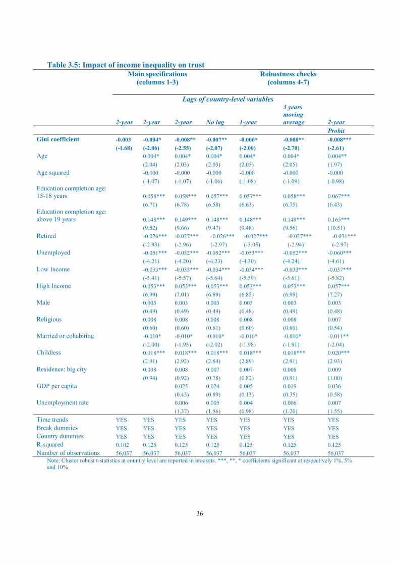
36

Table 3.5: Impact of income inequality on trust Main specifications

(columns 1-3)

Robustness checks (columns 4-7)

Lags of country-level variables

2-year 2-year 2-year

No lag 1-year

3 years moving average 2-year

Probit

Gini coefficient -0.003 -0.004* -0.008** -0.007** -0.006* -0.008** -0.008***

(-1.68) (-2.06) (-2.55) (-2.07) (-2.00) (-2.70) (-2.61)

Age 0.004* 0.004* 0.004* 0.004* 0.004* 0.004**

(2.04) (2.03) (2.03) (2.05) (2.05) (1.97)

Age squared -0.000 -0.000 -0.000 -0.000 -0.000 -0.000

(-1.07) (-1.07) (-1.06) (-1.08) (-1.09) (-0.98) Education completion age: 15-18 years 0.058*** 0.058*** 0.057*** 0.057*** 0.058*** 0.067***

(6.71) (6.78) (6.58) (6.63) (6.75) (6.43) Education completion age: above 19 years 0.148*** 0.149*** 0.148*** 0.148*** 0.149*** 0.165***

(9.52) (9.66) (9.47) (9.48) (9.56) (10.51)

Retired -0.026*** -0.027*** -0.026*** -0.027*** -0.027*** -0.031***

(-2.93) (-2.96) (-2.97) (-3.05) (-2.94) (-2.97)

Unemployed -0.051*** -0.052*** -0.052*** -0.053*** -0.052*** -0.060***

(-4.21) (-4.20) (-4.23) (-4.30) (-4.24) (-4.61)

Low Income -0.033*** -0.033*** -0.034*** -0.034*** -0.033*** -0.037***

(-5.41) (-5.57) (-5.64) (-5.59) (-5.61) (-5.82)

High Income 0.053*** 0.053*** 0.053*** 0.053*** 0.053*** 0.057***

(6.99) (7.01) (6.89) (6.85) (6.99) (7.27)

Male 0.003 0.003 0.003 0.003 0.003 0.003

(0.49) (0.49) (0.49) (0.48) (0.49) (0.48)

Religious 0.008 0.008 0.008 0.008 0.008 0.007

(0.60) (0.60) (0.61) (0.60) (0.60) (0.54)

Married or cohabiting -0.010* -0.010* -0.010* -0.010* -0.010* -0.011**

(-2.00) (-1.95) (-2.02) (-1.98) (-1.91) (-2.04)

Childless 0.018*** 0.018*** 0.018*** 0.018*** 0.018*** 0.020***

(2.91) (2.92) (2.84) (2.89) (2.91) (2.93)

Residence: big city 0.008 0.008 0.007 0.007 0.008 0.009

(0.94) (0.92) (0.78) (0.82) (0.91) (1.00)

GDP per capita 0.025 0.024 0.005 0.019 0.036

(0.45) (0.89) (0.13) (0.35) (0.58)

Unemployment rate 0.006 0.005 0.004 0.006 0.007

(1.37) (1.56) (0.98) (1.20) (1.55)

Time trends YES YES YES YES YES YES YES

Break dummies YES YES YES YES YES YES YES

Country dummies YES YES YES YES YES YES YES

R-squared 0.102 0.125 0.125 0.125 0.125 0.125 0.125

Number of observations 56,037 56,037 56,037 56,037 56,037 56,037 56,037 Note: Cluster robust t-statistics at country level are reported in brackets. ***, **, * coefficients significant at respectively 1%, 5% and 10%.

37

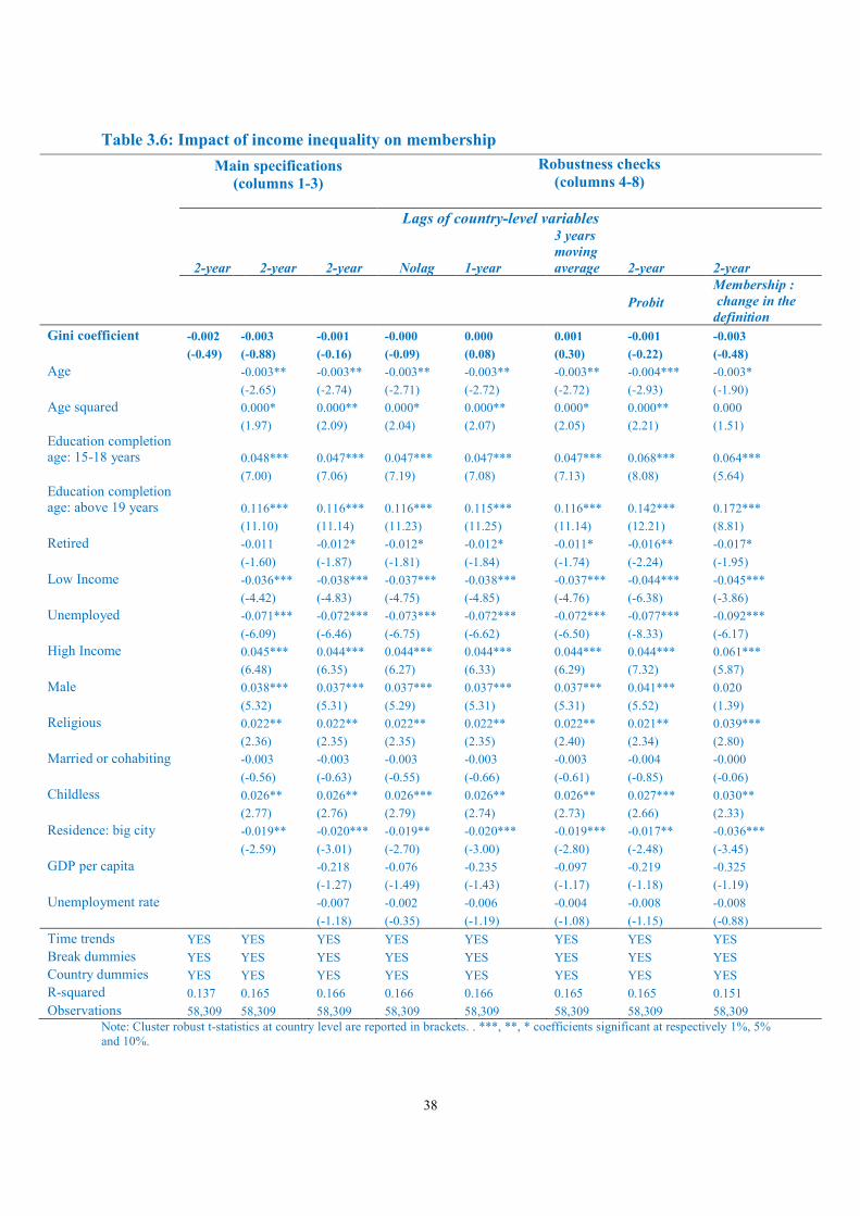
Membership and income inequality

Results reported in Table 3.6 show the association between social capital and income inequality

when social capital is measured by the participation in “Putnamesque”. The coefficient

associated with the Gini coefficient is not significantly different from zero, irrespective of the

covariates included in the analysis. This suggests that participation in associational activity is not

affected by the country level of income disparities. In columns 4-8, we present further estimates

of the relationship between membership and income inequality. Column 4 displays the results

when the Gini coefficient and the macroeconomic variables are contemporaneous to the

dependent variable while column 5 reports the estimates when both the Gini coefficient and the

macroeconomic variables are lagged one year. In column 6, we use a three years moving average

centered at t-2 for the Gini coefficient and the two macroeconomic variables. In column 7, we

have re-estimated equation (3.1) using a probit model. The conclusion regarding the association

between membership and income inequality remains unchanged. Finally, we have also checked

if the results concerning the effect of income inequality on associational activity are modified

when the membership indicator used so far is replaced by the cumulative number of

“Putnamesque” organizations to which each respondent belongs to. Again we do not find any

relationship between membership and income inequality.

Membership and the other covariates

The discussion below relies on the estimations presented in column 3 of Table 3.6. As for the

membership indicator, we find that education is a significant determinant of participation in

associational activities. The magnitude of the estimated coefficients of the two education

dummies are strikingly similar to those observed for trust. Being unemployed reduces

participation in associations by 7%. Given that we also control for individual income, this result

suggests that the unemployment status is detrimental per se for the formation of social capital (i.e.

not only through the income loss associated with it).

38

Table 3.6: Impact of income inequality on membership

Note: Cluster robust t-statistics at country level are reported in brackets. . ***, **, * coefficients significant at respectively 1%, 5% and 10%.

Main specifications (columns 1-3)

Robustness checks (columns 4-8)

Lags of country-level variables

2-year 2-year 2-year Nolag 1-year

3 years moving average 2-year 2-year

Probit

Membership : change in the definition

Gini coefficient -0.002 -0.003 -0.001 -0.000 0.000 0.001 -0.001 -0.003

(-0.49) (-0.88) (-0.16) (-0.09) (0.08) (0.30) (-0.22) (-0.48)

Age -0.003** -0.003** -0.003** -0.003** -0.003** -0.004*** -0.003*

(-2.65) (-2.74) (-2.71) (-2.72) (-2.72) (-2.93) (-1.90)

Age squared 0.000* 0.000** 0.000* 0.000** 0.000* 0.000** 0.000

(1.97) (2.09) (2.04) (2.07) (2.05) (2.21) (1.51) Education completion age: 15-18 years 0.048*** 0.047*** 0.047*** 0.047*** 0.047*** 0.068*** 0.064***

(7.00) (7.06) (7.19) (7.08) (7.13) (8.08) (5.64) Education completion age: above 19 years 0.116*** 0.116*** 0.116*** 0.115*** 0.116*** 0.142*** 0.172***

(11.10) (11.14) (11.23) (11.25) (11.14) (12.21) (8.81)

Retired -0.011 -0.012* -0.012* -0.012* -0.011* -0.016** -0.017*

(-1.60) (-1.87) (-1.81) (-1.84) (-1.74) (-2.24) (-1.95)

Low Income -0.036*** -0.038*** -0.037*** -0.038*** -0.037*** -0.044*** -0.045***

(-4.42) (-4.83) (-4.75) (-4.85) (-4.76) (-6.38) (-3.86)

Unemployed -0.071*** -0.072*** -0.073*** -0.072*** -0.072*** -0.077*** -0.092***

(-6.09) (-6.46) (-6.75) (-6.62) (-6.50) (-8.33) (-6.17)

High Income 0.045*** 0.044*** 0.044*** 0.044*** 0.044*** 0.044*** 0.061***

(6.48) (6.35) (6.27) (6.33) (6.29) (7.32) (5.87)

Male 0.038*** 0.037*** 0.037*** 0.037*** 0.037*** 0.041*** 0.020

(5.32) (5.31) (5.29) (5.31) (5.31) (5.52) (1.39)

Religious 0.022** 0.022** 0.022** 0.022** 0.022** 0.021** 0.039***

(2.36) (2.35) (2.35) (2.35) (2.40) (2.34) (2.80)

Married or cohabiting -0.003 -0.003 -0.003 -0.003 -0.003 -0.004 -0.000

(-0.56) (-0.63) (-0.55) (-0.66) (-0.61) (-0.85) (-0.06)

Childless 0.026** 0.026** 0.026*** 0.026** 0.026** 0.027*** 0.030**

(2.77) (2.76) (2.79) (2.74) (2.73) (2.66) (2.33)

Residence: big city -0.019** -0.020*** -0.019** -0.020*** -0.019*** -0.017** -0.036***

(-2.59) (-3.01) (-2.70) (-3.00) (-2.80) (-2.48) (-3.45)

GDP per capita -0.218 -0.076 -0.235 -0.097 -0.219 -0.325

(-1.27) (-1.49) (-1.43) (-1.17) (-1.18) (-1.19)

Unemployment rate -0.007 -0.002 -0.006 -0.004 -0.008 -0.008

(-1.18) (-0.35) (-1.19) (-1.08) (-1.15) (-0.88)

Time trends YES YES YES YES YES YES YES YES

Break dummies YES YES YES YES YES YES YES YES

Country dummies YES YES YES YES YES YES YES YES

R-squared 0.137 0.165 0.166 0.166 0.166 0.165 0.165 0.151

Observations 58,309 58,309 58,309 58,309 58,309 58,309 58,309 58,309

39

Contrary to the findings of the trust equation, males, religious and childless individuals display

higher levels of participation in “putnamesque” organizations. In addition, respondents living in

big cities are around 2% more likely to participate in associational activities..

Finally, the GDP per capita and the unemployment rate are not significantly different from zero

in explaining the probability of participating in associational activities.21 These findings suggest

that compositional changes in income and employment have no effect on membership, when the

individual heterogeneity is taken into account.

The empirical analysis presented in this chapter suggests heterogeneous results. On the one hand,

income inequality appears to be negatively and significantly associated with trust, and this

relationship is robust to several specifications. On the other hand, participation in associational

activities does not show any statistically significant correlation with income disparities.

21 As we state in the preceding section, this is probably the result of controlling concurrently for the country fixed effects and the macroeconomic variables.

40

4. The impact of income inequality on happiness

4.1 The rationale

The discussion on whether income inequality affects an individual's happiness dates back to

theoretical considerations on relative deprivation and relative utility and refers to the idea that

people's utility depends not only on their own income but also on their relative position in the

society (van de Stadt, Kapteyn and van de Geer, 1985). In addition, some scholars suggest that

individuals can have a “taste for equality”. In particular, Thurow (1971, p.327) proposes that “the

individual is simply exercising an aesthetic taste for equality or inequality similar in nature to a

taste for paintings”.

An intuitive and comprehensive explanation of the impact of income inequality on individuals'

well-being is provided by Hirschman and Rothschild (1973). These authors use the analogy of a

traffic jam on a two-lane motorway to explain the effect of income inequality on happiness and

call this the “tunnel effect”' (Hirschman and Rothschild (1973), p.545):

“Suppose that I drive through a two-lane tunnel, both lanes going the same direction,

and run into a serious traffic jam. No car is moving in either lane as far as I can see

(which is not very far). I am in the left lane and feel dejected. After a while the cars

in the right lane begin to move. Naturally, my spirits lift considerably, for I know

that the jam has been broken and that my lane's turn to move will surely come any

moment now. But suppose that the expectation is disappointed and only the right

lane keeps moving: in that case I will at some point become quite furious”.

This analogy nicely illustrates several important aspects in the relationship between income

inequality and happiness. First, inequality may convey information about future prospects. This

means that if I observe that the people around me are moving, then I expect to be able to move

upward soon too. This suggests that income inequality might have a positive effect on

individuals' wellbeing.

Second, the positive impact of inequality might turn negative if these expectations are not

fulfilled, i.e. if my lane is still not moving. This has important consequences for countries in

41

different development stages and there is empirical evidence on transition countries supporting

this notion (as discussed below).

Last, the question arises at what point people do get “upset” about their lane not moving. This

refers to people's beliefs on whether mobility is possible in their country and how difficult it is

for people to move upwards.

In conclusion, income inequality might affect positively the individual's level of happiness if

people perceive that in their society upward mobility is possible. However, if individuals think

that it is very unlikely to reach a higher income, then income inequality will probably impact

negatively on happiness.

4.2 Existing empirical evidence

There exists quite substantial empirical evidence on the impact of income inequality on

happiness or life satisfaction, mainly covering the U.S., Europe and transition countries (for an

overview see Table 4.1). As anticipated theoretically, the effect of income inequality on

happiness critically depends on whether (i) individuals perceive the society open to upward

mobility and (ii) it is likely that they will eventually be able to reach higher income levels.

Evidence can thus be divided into the low-mobile countries (typically European), where

inequality has a negative effect on satisfaction, and the highly mobile society such as the U.S.

and transition countries, where there seems to be a greater variability in the outcomes of income

inequality.

For European countries, Senik (2006) finds that inequality has a negative effect on life

satisfaction. Alesina et al. (2004) show that this result is driven by the detrimental effect of

income inequality on people with low income and to those belonging to the left ideological

spectrum. On the contrary, richer individuals seem indifferent about income inequality.

Schwarze and Harpfer (2007) report that income inequality has a negative effect on life

satisfaction in Germany, while Ferrer-i-Carbonell (2005) show that the higher the income of the

reference group is, the lower is the level of happiness. Clark (2006) reports similar findings for

Britain while using life satisfaction as the outcome. Additionally, Clark (2006) argues that higher

42

income inequality within the reference group actually increases life satisfaction. The latter effect

might convey some form of ‘opportunity’ feeling similar to some of the findings in the U.S.

The evidence for the U.S. is somewhat mixed. Senik (2006) conclude that, in contrast to the

evidence from Europe, inequality in the U.S. has a positive effect on life satisfaction. This result

is challenged by evidence provided by McBride (2001), Luttmer (2005), and Dynan and Ravina

(2007). These scholars report that a higher ‘reference group income’ negatively affects happiness.

A more nuanced view can be found in Alesina et al. (2004), who investigate different income

levels and incorporate the political preferences of individuals. Their finding is that in the U.S. it

is the rich people, who are particularly unhappy about higher levels of income inequality,

whereas the poor are indifferent to inequality. Hence, some of the contrasting evidence might be

explained by different samples of individuals.

Last, several studies exist on the impact of inequality on happiness in transition countries. While

Sanfey and Teksoz (2005) show that inequality has a negative impact on life satisfaction in

various transition countries, Senik (2006) conclude that the income of the reference group and

the level of satisfaction are positively related in transition countries. Moreover, the author

provides evidence that this effect is particularly strong for younger people, i.e. below 41 years,

and for individuals, who experienced higher income volatility. Similarly, for Russia, Senik (2004)

finds a positive impact of the ‘reference group income’ on life satisfaction and no significant

effect for income inequality. The variability of the results is confirmed in Grosfeld and Senik’s

(2008) study on Poland. Here, the authors find that there has been a major structural change in

the perception of income inequality after 1997. Before 1997, income inequality is positively

associated with life satisfaction and individual’s expectations about the future. After 1997,

however, income inequality is not significantly associated anymore with life satisfaction. This is

explained by the perception of Polish people that they were not benefitting from the economic

transformation.

In conclusion, empirical evidence strongly suggests that the perception of income inequality as a

negative force in the society depends critically on the perceived country mobility and might

differ by income group, political preferences, and age. For Europe, a negative impact of income

inequality or of the ‘reference group income’ on happiness is observed. Transition between

43

political regimes may render the association inequality/happiness positive or negative in time

depending on the level of expectation raised and their possible fulfillment or delusion.

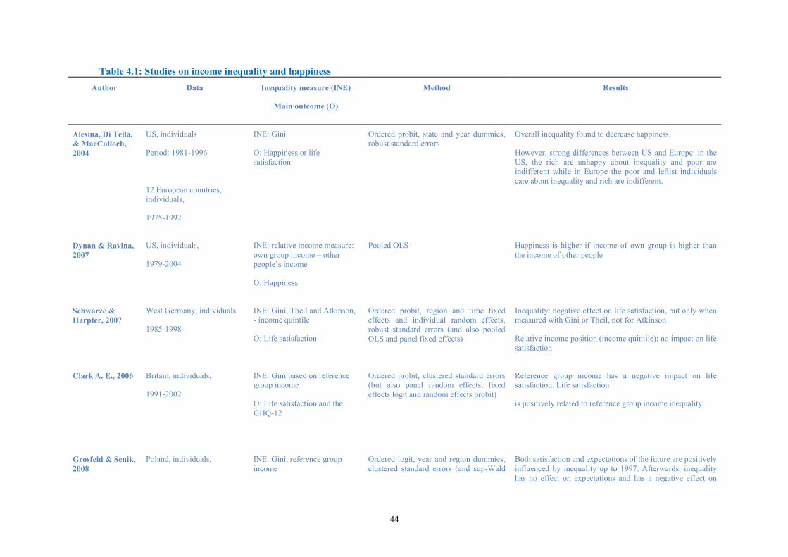
44

Table 4.1: Studies on income inequality and happiness

Author Data Inequality measure (INE)

Main outcome (O)

Method Results

Alesina, Di Tella, & MacCulloch, 2004

US, individuals

Period: 1981-1996

12 European countries, individuals,

1975-1992

INE: Gini

O: Happiness or life satisfaction

Ordered probit, state and year dummies, robust standard errors

Overall inequality found to decrease happiness.

However, strong differences between US and Europe: in the US, the rich are unhappy about inequality and poor are indifferent while in Europe the poor and leftist individuals care about inequality and rich are indifferent.

Dynan & Ravina, 2007

US, individuals,

1979-2004

INE: relative income measure: own group income – other people’s income

O: Happiness

Pooled OLS Happiness is higher if income of own group is higher than the income of other people

Schwarze & Harpfer, 2007

West Germany, individuals

1985-1998

INE: Gini, Theil and Atkinson, - income quintile

O: Life satisfaction

Ordered probit, region and time fixed effects and individual random effects, robust standard errors (and also pooled OLS and panel fixed effects)

Inequality: negative effect on life satisfaction, but only when measured with Gini or Theil, not for Atkinson

Relative income position (income quintile): no impact on life satisfaction

Clark A. E., 2006 Britain, individuals,

1991-2002

INE: Gini based on reference group income

O: Life satisfaction and the GHQ-12

Ordered probit, clustered standard errors (but also panel random effects, fixed effects logit and random effects probit)

Reference group income has a negative impact on life satisfaction. Life satisfaction

is positively related to reference group income inequality.

Grosfeld & Senik, 2008

Poland, individuals, INE: Gini, reference group income

Ordered logit, year and region dummies, clustered standard errors (and sup-Wald

Both satisfaction and expectations of the future are positively influenced by inequality up to 1997. Afterwards, inequality has no effect on expectations and has a negative effect on

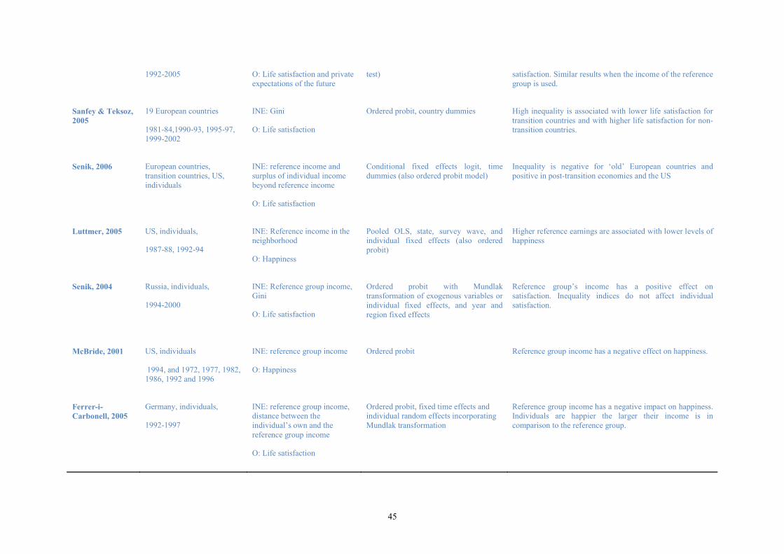
45

1992-2005 O: Life satisfaction and private expectations of the future

test) satisfaction. Similar results when the income of the reference group is used.

Sanfey & Teksoz, 2005

19 European countries

1981-84,1990-93, 1995-97, 1999-2002

INE: Gini

O: Life satisfaction

Ordered probit, country dummies High inequality is associated with lower life satisfaction for transition countries and with higher life satisfaction for non-transition countries.

Senik, 2006 European countries, transition countries, US, individuals

INE: reference income and surplus of individual income beyond reference income

O: Life satisfaction

Conditional fixed effects logit, time dummies (also ordered probit model)

Inequality is negative for ‘old’ European countries and positive in post-transition economies and the US

Luttmer, 2005 US, individuals,

1987-88, 1992-94

INE: Reference income in the neighborhood

O: Happiness

Pooled OLS, state, survey wave, and individual fixed effects (also ordered probit)

Higher reference earnings are associated with lower levels of happiness

Senik, 2004 Russia, individuals,

1994-2000

INE: Reference group income, Gini

O: Life satisfaction

Ordered probit with Mundlak transformation of exogenous variables or individual fixed effects, and year and region fixed effects

Reference group’s income has a positive effect on satisfaction. Inequality indices do not affect individual satisfaction.

McBride, 2001 US, individuals

1994, and 1972, 1977, 1982, 1986, 1992 and 1996

INE: reference group income

O: Happiness

Ordered probit Reference group income has a negative effect on happiness.

Ferrer-i-Carbonell, 2005

Germany, individuals,

1992-1997

INE: reference group income, distance between the individual’s own and the reference group income

O: Life satisfaction

Ordered probit, fixed time effects and individual random effects incorporating Mundlak transformation

Reference group income has a negative impact on happiness. Individuals are happier the larger their income is in comparison to the reference group.

46

4.3 Empirical analysis

4.3.1 Happiness variable

The happiness variable is taken from the European Value Survey (EVS) and is related to

the following question: “Taking all things together, would you say you are: very happy,

quite happy, not very happy, or not at all happy". The indicator ranges from 4, i.e. very

happy, to 1, i.e. not at all happy. This measure of happiness is the most commonly used

in the existing literature.

In the empirical analysis, we have collapsed the four categories into two categories so as

to create a dummy variable which takes the value one if the individuals report that they

feel “very/quite happy”, and zero otherwise. The reasons to proceed in such a way are the

following.. First, respondents seem not to be evenly distributed across the 4 scores and

hence this might affect the representativeness of the sample in the different countries.

Second, as it will be explained below, statistically speaking, there is no difference

between the categories 1 and 2, i.e. “not at all happy” and “not too happy”, as well as

between the categories 3 and 4, i.e., “quite happy’ and “very happy”.

Chart 4.1 shows the country share of individuals that report a high value of the happiness

indicator (i.e., reporting to be “quite/very happy”). There are stark differences across

European Member States and these variations suggest a regional clustering. In fact,

excluding Czech Republic, all Eastern European countries report the lowest level of

happiness, while Nordic countries (Sweden, Denmark, the Netherlands) along with

Ireland display the highest level of happiness.

Chart 4.2 and Table 4.2 provide further information on the evolution over time of the

share of people reporting high scores of happiness. Chart 4.2 shows the regression line

when the country-wave specific level of happiness is fitted against a trend. After having

partialled out for the country fixed effects, the proportion of people reporting to be

‘‘quite/very happy” has, on average, increased by 0.06 % between each wave.

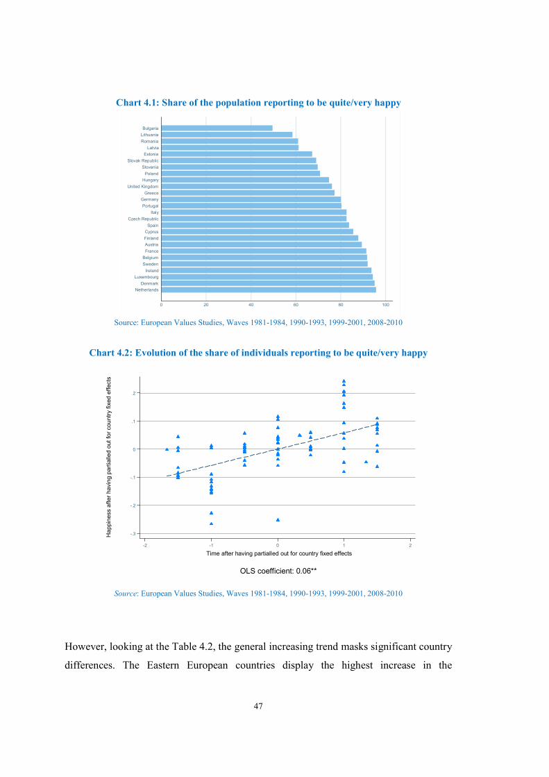
47

Chart 4.1: Share of the population reporting to be quite/very happy

Source: European Values Studies, Waves 1981-1984, 1990-1993, 1999-2001, 2008-2010

Chart 4.2: Evolution of the share of individuals reporting to be quite/very happy

Source: European Values Studies, Waves 1981-1984, 1990-1993, 1999-2001, 2008-2010

However, looking at the Table 4.2, the general increasing trend masks significant country

differences. The Eastern European countries display the highest increase in the

0 20 40 60 80 100

Netherlands

Denmark

Luxembourg

Ireland

Sweden

Belgium

France

Austria

Finland

Cyprus

Spain

Czech Republic

Italy

Portugal

Germany

Greece

United Kingdom

Hungary

Poland

Slovenia

Slovak Republic

Estonia

Latvia

Romania

Lithuania

Bulgaria

-.3

-.2

-.1

0

.1

.2

Happin

ess

aft

er

havi

ng p

art

ialle

d o

ut

for

countr

y fixe

d e

ffect

s

-2 -1 0 1 2

Time after having partialled out for country fixed effects

OLS coefficient: 0.06**

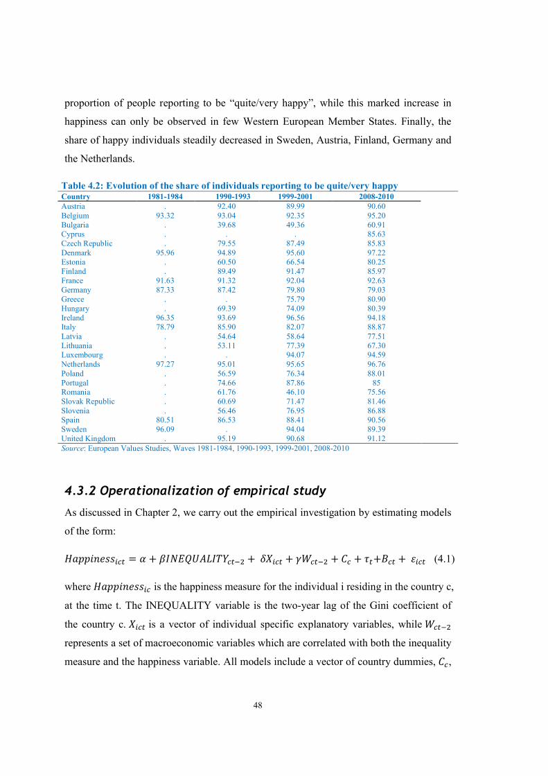
48

proportion of people reporting to be “quite/very happy”, while this marked increase in

happiness can only be observed in few Western European Member States. Finally, the

share of happy individuals steadily decreased in Sweden, Austria, Finland, Germany and

the Netherlands.

Table 4.2: Evolution of the share of individuals reporting to be quite/very happy Country 1981-1984 1990-1993 1999-2001 2008-2010 Austria . 92.40 89.99 90.60 Belgium 93.32 93.04 92.35 95.20 Bulgaria . 39.68 49.36 60.91 Cyprus . . . 85.63 Czech Republic . 79.55 87.49 85.83 Denmark 95.96 94.89 95.60 97.22 Estonia . 60.50 66.54 80.25 Finland . 89.49 91.47 85.97 France 91.63 91.32 92.04 92.63 Germany 87.33 87.42 79.80 79.03 Greece . . 75.79 80.90 Hungary . 69.39 74.09 80.39 Ireland 96.35 93.69 96.56 94.18 Italy 78.79 85.90 82.07 88.87 Latvia . 54.64 58.64 77.51 Lithuania . 53.11 77.39 67.30 Luxembourg . . 94.07 94.59 Netherlands 97.27 95.01 95.65 96.76 Poland . 56.59 76.34 88.01 Portugal . 74.66 87.86 85 Romania . 61.76 46.10 75.56 Slovak Republic . 60.69 71.47 81.46 Slovenia . 56.46 76.95 86.88 Spain 80.51 86.53 88.41 90.56 Sweden 96.09 . 94.04 89.39 United Kingdom . 95.19 90.68 91.12 Source: European Values Studies, Waves 1981-1984, 1990-1993, 1999-2001, 2008-2010

4.3.2 Operationalization of empirical study

As discussed in Chapter 2, we carry out the empirical investigation by estimating models

of the form:

������������ = � + ��������������� +����� + ������ + �� + ��+��� + ���� (4.1)

where ����������� is the happiness measure for the individual i residing in the country c,

at the time t. The INEQUALITY variable is the two-year lag of the Gini coefficient of

the country c. ���� is a vector of individual specific explanatory variables, while �����

represents a set of macroeconomic variables which are correlated with both the inequality

measure and the happiness variable. All models include a vector of country dummies, ��,

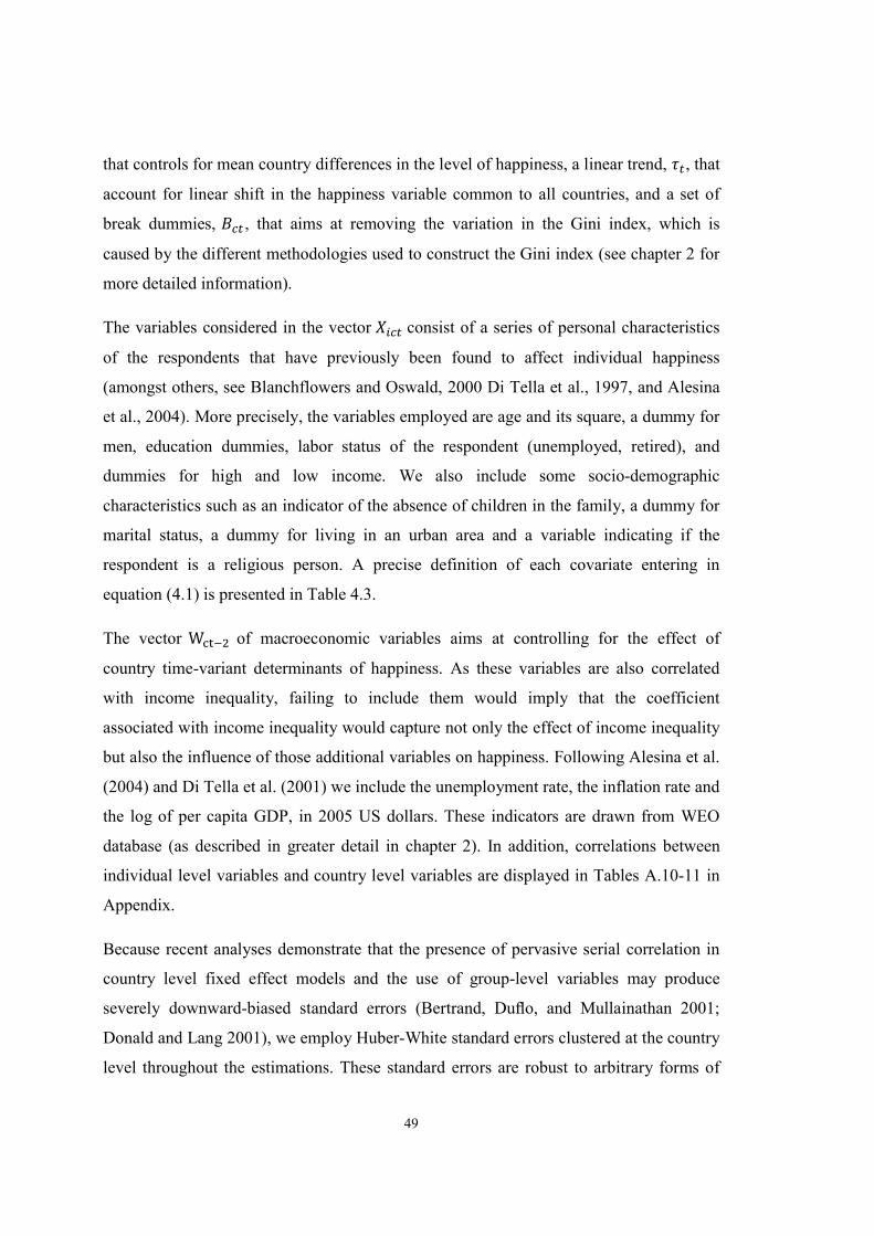
49

that controls for mean country differences in the level of happiness, a linear trend, ��, that

account for linear shift in the happiness variable common to all countries, and a set of

break dummies, ��� , that aims at removing the variation in the Gini index, which is

caused by the different methodologies used to construct the Gini index (see chapter 2 for

more detailed information).

The variables considered in the vector ���� consist of a series of personal characteristics

of the respondents that have previously been found to affect individual happiness

(amongst others, see Blanchflowers and Oswald, 2000 Di Tella et al., 1997, and Alesina

et al., 2004). More precisely, the variables employed are age and its square, a dummy for

men, education dummies, labor status of the respondent (unemployed, retired), and

dummies for high and low income. We also include some socio-demographic

characteristics such as an indicator of the absence of children in the family, a dummy for

marital status, a dummy for living in an urban area and a variable indicating if the

respondent is a religious person. A precise definition of each covariate entering in

equation (4.1) is presented in Table 4.3.

The vector W���� of macroeconomic variables aims at controlling for the effect of

country time-variant determinants of happiness. As these variables are also correlated

with income inequality, failing to include them would imply that the coefficient

associated with income inequality would capture not only the effect of income inequality

but also the influence of those additional variables on happiness. Following Alesina et al.

(2004) and Di Tella et al. (2001) we include the unemployment rate, the inflation rate and

the log of per capita GDP, in 2005 US dollars. These indicators are drawn from WEO

database (as described in greater detail in chapter 2). In addition, correlations between

individual level variables and country level variables are displayed in Tables A.10-11 in

Appendix.

Because recent analyses demonstrate that the presence of pervasive serial correlation in

country level fixed effect models and the use of group-level variables may produce

severely downward-biased standard errors (Bertrand, Duflo, and Mullainathan 2001;

Donald and Lang 2001), we employ Huber-White standard errors clustered at the country

level throughout the estimations. These standard errors are robust to arbitrary forms of

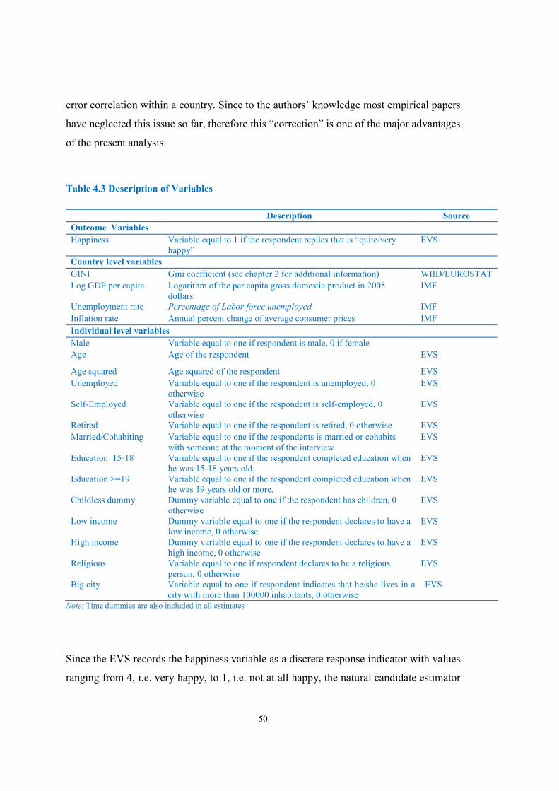
50

error correlation within a country. Since to the authors’ knowledge most empirical papers

have neglected this issue so far, therefore this “correction” is one of the major advantages

of the present analysis.

Table 4.3 Description of Variables

Description Source

Outcome Variables

Happiness Variable equal to 1 if the respondent replies that is “quite/very happy”

EVS

Country level variables

GINI Gini coefficient (see chapter 2 for additional information) WIID/EUROSTAT

Log GDP per capita Logarithm of the per capita gross domestic product in 2005 dollars

IMF

Unemployment rate Percentage of Labor force unemployed IMF

Inflation rate Annual percent change of average consumer prices IMF

Individual level variables

Male Variable equal to one if respondent is male, 0 if female

Age Age of the respondent EVS

Age squared Age squared of the respondent EVS

Unemployed Variable equal to one if the respondent is unemployed, 0 otherwise

EVS

Self-Employed Variable equal to one if the respondent is self-employed, 0 otherwise

EVS

Retired Variable equal to one if the respondent is retired, 0 otherwise EVS

Married/Cohabiting Variable equal to one if the respondents is married or cohabits with someone at the moment of the interview

EVS

Education 15-18 Variable equal to one if the respondent completed education when he was 15-18 years old,

EVS

Education >=19 Variable equal to one if the respondent completed education when he was 19 years old or more,

EVS

Childless dummy Dummy variable equal to one if the respondent has children, 0 otherwise

EVS

Low income Dummy variable equal to one if the respondent declares to have a low income, 0 otherwise

EVS

High income Dummy variable equal to one if the respondent declares to have a high income, 0 otherwise

EVS

Religious Variable equal to one if respondent declares to be a religious person, 0 otherwise

EVS

Big city Variable equal to one if respondent indicates that he/she lives in a city with more than 100000 inhabitants, 0 otherwise

EVS

Note: Time dummies are also included in all estimates

Since the EVS records the happiness variable as a discrete response indicator with values

ranging from 4, i.e. very happy, to 1, i.e. not at all happy, the natural candidate estimator

51

for the equation (1) would be a maximum likelihood estimator for ordered dependent

variable, namely ordered probit/logit. In fact, we started the empirical analysis estimating

equation (1) by using an ordered probit model. Other than giving the estimated

coefficients of the control variables, the ordered probit model estimates the cut points

(and the corresponding standard errors) between the response outcomes, i.e. the

thresholds that the latent continuous variable must cross to change the value of the

corresponding happiness discrete variable. These estimated parameters are crucial for

testing the relevance of the 4-scores happiness variable.

The results show that only the 2nd and the 3rd cut point are statistically different from

zero22 , suggesting that we can rule out the lowest category referring to individuals

reporting themselves as “not at all happy”23. In addition, by looking at the confidence

bounds of the thresholds we can also discard the discontinuity between the “quite happy”

and “very happy” category (the upper bound of cut2, equal to 5.82, lies far above the

lower bound of cut3, which is equal to 2.3). This leaves us with the 2nd cut point to be the

only statistically relevant threshold. For these reasons, we refrain from using the 4-scores

variable and instead we apply the binary version of the happiness variable. As a result,

the dependent variable of equation (4.1) takes on the value one if people report to be

“quite/very happy” and zero otherwise. We estimate equation (4.1) using ordinary least

squares and provide the probit estimates as a robustness exercise.24 Furthermore, we also

report results when a measure of life satisfaction is the dependent variable. Although

happiness and life satisfaction might capture different aspects of individual wellbeing,

they are highly correlated, showing a correlation coefficient above 0.75. As a result, we

do not expect to detect any relevant differences between the two models.25

22 cut 2: 3.09 s.e.:(1.39); cut 3: 5.02 s.e.:(1.38)

23 cut 1: 1.9 s.e.:(1.38)

24 Note that the OLS coefficients are readily interpretable as marginal effects at the mean of the other covariates.

25 The EVS measures individual life satisfaction as a discrete response variable with values ranging from 10, i.e. very satisfied, to 1, i.e. not at all satisfied. However, for comparison’s sake, we have estimated the model using the binary version of the life satisfaction score.

52

4.3.3 Econometric results

Table 4.4 presents the estimated coefficients of the equation (4.1). Columns 1-3 show the

results of the models where the income inequality is measured by the 2-year lag of the

Gini coefficient. Model 1 is the baseline estimate that controls only for country and break

dummies, a linear time trend and the Gini coefficient. Model 2 includes a series of

individual characteristics which have previously been found to affect individual

happiness, while model 3 considers macroeconomic confounding variables which may

potentially be correlated with both the Gini coefficient and individual happiness. Note

that since the Gini coefficient is fixed within country-year clusters, only country-specific

variables are likely to be a source of omitted variable bias. This is the main reason of

including the macroeconomic controls in model 3.

In order to mitigate the potential issues of reverse causation, the Gini coefficient enter the

equation with 2-year lag. Although this presents a deviation from the existing literature,

which usually relies on contemporaneous measure of the Gini index, we think that the

level of happiness might be influenced by income inequality in the past years. However,

for the sake of comparison with the previous literature we also estimate the equation (4.1)

including the contemporaneous Gini. This model is shown in column 4 of Table 4.4. In

addition, in column 5 we present estimation results using the unweighted three-year

moving average of the Gini index. Lastly, column 7 reports the model when life

satisfaction is the dependent variable.

The estimates reported in column 1 of Table 4.4 show the estimated impact of the

inequality on the individual happiness. The coefficient of the Gini equals to 0.009. This

indicates that a 1% rise in the Gini coefficient increases the proportion of people

reporting to be “quite/very happy” by 0.009 percentage points. Although very small, this

result is neither consistent with our prior expectations nor with empirical results from

previous research. However, this impact is estimated imprecisely. The second column

adds a series of individual characteristics to the estimation model. The added control

variables are economically and statistically significant with “standard” interpretations

and in line with the previous literature. For instance, we find an inverted U-shaped effect

53

of age on happiness, i.e. younger people seem to be the least happy compared to the older

ones. Having completed education at the age of 19 is associated with higher levels of

happiness, as shown by the coefficient on education. Being unemployed and retired are

associated with lower levels of happiness. A possible interpretation might be that these

labour status are correlated with the stress of being jobless. The income dummies clearly

show that money matters: earning a higher income brings happiness. Men seem not to be

happier than women and following a religion makes people happier. Regarding the

marital status, we find that married or cohabiting people are happier than unmarried or

single ones. In addition, people seem to be less happy if they have at least one child. This

lower level of happiness for individuals with children might be caused by the

preoccupations and responsibilities associated with raising children.

Column 2 of Table 4.4 shows a positive effect of the Gini index on individual happiness.

However, this counterintuitive effect might be determined by endogeneity of the Gini

variable, especially the one coming from omitted country determinants of both inequality

and individual happiness. To tackle this issue, in column 3 we add the following

macroeconomic variables in the model: unemployment rate, inflation rate and per capita

GDP. The Gini coefficient turns negatively correlated with the individual level of

happiness with a magnitude of -0.004, validating our suspect that the previous models are

strongly affected by omitted variable bias. Indeed, the coefficient of per capita GDP is

strongly statistically significant, suggesting that the positive effect of the Gini index in

column 3 stems mainly from the omission of this macroeconomic variable. However the

negative effect of the Gini is far from being statistically significant.

Column 5 shows the estimated coefficients where both the Gini measure and the

macroeconomic variables are calculated as unweighted three-year moving average,

centered at year t-1. The estimated coefficient of the income inequality becomes smaller,

moving from -0.004 in column 3 to -0.001, and negatively associated with individual

wellbeing, but still not statistical different from zero.

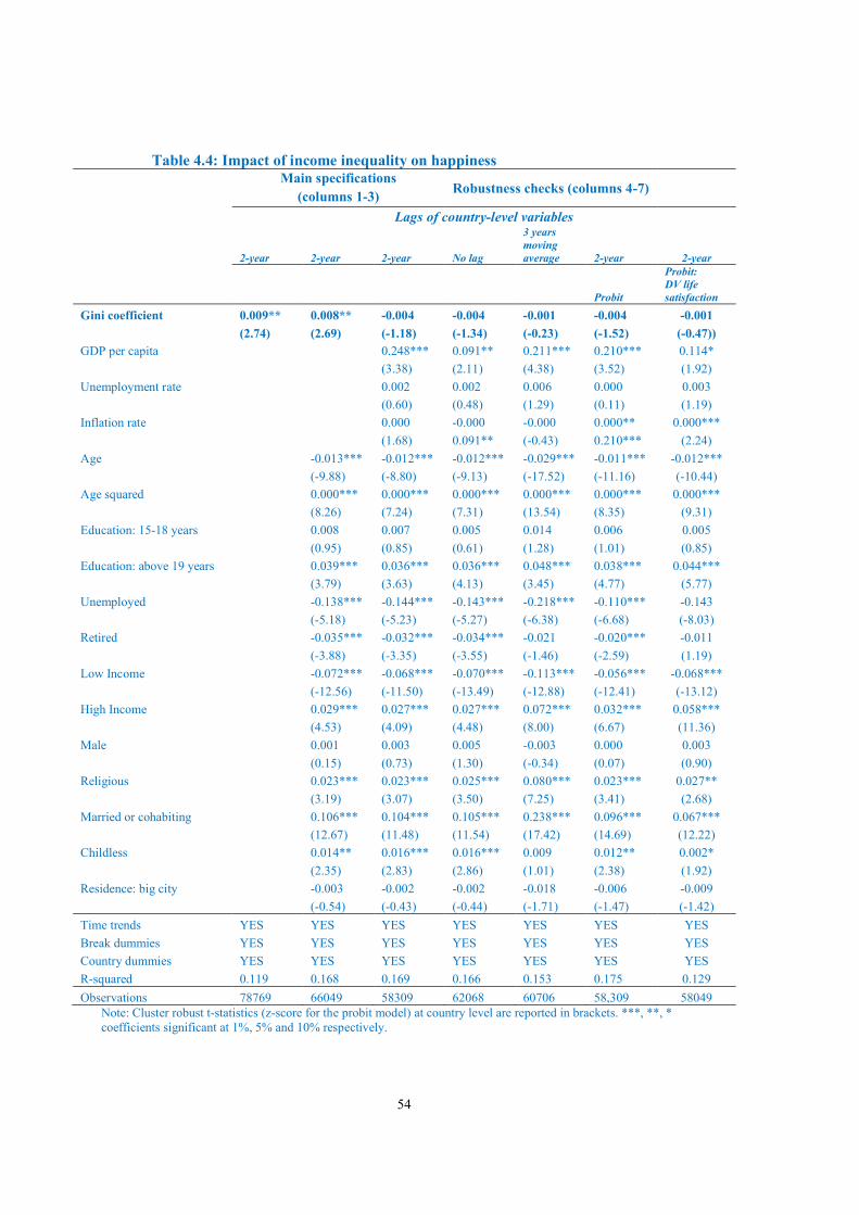
54

Table 4.4: Impact of income inequality on happiness

Main specifications

(columns 1-3) Robustness checks (columns 4-7)

Lags of country-level variables

2-year 2-year 2-year No lag

3 years moving average 2-year 2-year

Probit

Probit: DV life satisfaction

Gini coefficient 0.009** 0.008** -0.004 -0.004 -0.001 -0.004 -0.001

(2.74) (2.69) (-1.18) (-1.34) (-0.23) (-1.52) (-0.47))

GDP per capita 0.248*** 0.091** 0.211*** 0.210*** 0.114*

(3.38) (2.11) (4.38) (3.52) (1.92)

Unemployment rate 0.002 0.002 0.006 0.000 0.003

(0.60) (0.48) (1.29) (0.11) (1.19)

Inflation rate 0.000 -0.000 -0.000 0.000** 0.000***

(1.68) 0.091** (-0.43) 0.210*** (2.24)

Age -0.013*** -0.012*** -0.012*** -0.029*** -0.011*** -0.012***

(-9.88) (-8.80) (-9.13) (-17.52) (-11.16) (-10.44)

Age squared 0.000*** 0.000*** 0.000*** 0.000*** 0.000*** 0.000***

(8.26) (7.24) (7.31) (13.54) (8.35) (9.31)

Education: 15-18 years 0.008 0.007 0.005 0.014 0.006 0.005

(0.95) (0.85) (0.61) (1.28) (1.01) (0.85)

Education: above 19 years 0.039*** 0.036*** 0.036*** 0.048*** 0.038*** 0.044***

(3.79) (3.63) (4.13) (3.45) (4.77) (5.77)

Unemployed -0.138*** -0.144*** -0.143*** -0.218*** -0.110*** -0.143

(-5.18) (-5.23) (-5.27) (-6.38) (-6.68) (-8.03)

Retired -0.035*** -0.032*** -0.034*** -0.021 -0.020*** -0.011

(-3.88) (-3.35) (-3.55) (-1.46) (-2.59) (1.19)

Low Income -0.072*** -0.068*** -0.070*** -0.113*** -0.056*** -0.068***

(-12.56) (-11.50) (-13.49) (-12.88) (-12.41) (-13.12)

High Income 0.029*** 0.027*** 0.027*** 0.072*** 0.032*** 0.058***

(4.53) (4.09) (4.48) (8.00) (6.67) (11.36)

Male 0.001 0.003 0.005 -0.003 0.000 0.003

(0.15) (0.73) (1.30) (-0.34) (0.07) (0.90)

Religious 0.023*** 0.023*** 0.025*** 0.080*** 0.023*** 0.027**

(3.19) (3.07) (3.50) (7.25) (3.41) (2.68)

Married or cohabiting 0.106*** 0.104*** 0.105*** 0.238*** 0.096*** 0.067***

(12.67) (11.48) (11.54) (17.42) (14.69) (12.22)

Childless 0.014** 0.016*** 0.016*** 0.009 0.012** 0.002*

(2.35) (2.83) (2.86) (1.01) (2.38) (1.92)

Residence: big city -0.003 -0.002 -0.002 -0.018 -0.006 -0.009

(-0.54) (-0.43) (-0.44) (-1.71) (-1.47) (-1.42)

Time trends YES YES YES YES YES YES YES

Break dummies YES YES YES YES YES YES YES

Country dummies YES YES YES YES YES YES YES

R-squared 0.119 0.168 0.169 0.166 0.153 0.175 0.129

Observations 78769 66049 58309 62068 60706 58,309 58049 Note: Cluster robust t-statistics (z-score for the probit model) at country level are reported in brackets. ***, **, * coefficients significant at 1%, 5% and 10% respectively.

55

In column 6 we analyse whether our results might be affected by the functional form of

the estimated model. In particular, we investigate whether the probit model, which

assumes a nonlinear functional form between the explanatory variables and the

dependent variable, is better suited to estimate equation (1). The marginal effects of the

probit model reported in column 6 of Table 4.3 are unambiguously similar to the

coefficient of the model 3, suggesting that the functional form is not a serious concern.

Likewise, the coefficient of the Gini index remains statistically insignificant with a

magnitude of -0.004.

Finally, we obtain similar results when individual wellbeing is proxied by life satisfaction

dummy variable (column 7). The coefficient attached to the Gini index is negatively

related to wellbeing but still not statistically significant.

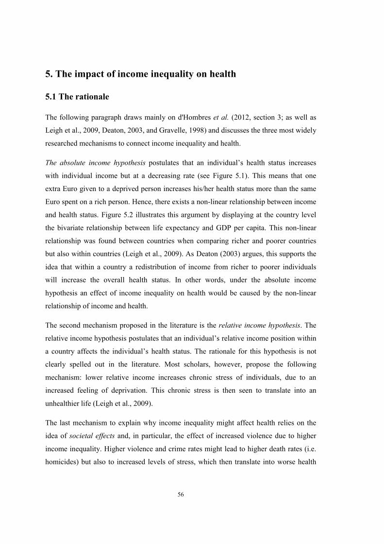
56

5. The impact of income inequality on health

5.1 The rationale

The following paragraph draws mainly on d'Hombres et al. (2012, section 3; as well as

Leigh et al., 2009, Deaton, 2003, and Gravelle, 1998) and discusses the three most widely

researched mechanisms to connect income inequality and health.

The absolute income hypothesis postulates that an individual’s health status increases

with individual income but at a decreasing rate (see Figure 5.1). This means that one

extra Euro given to a deprived person increases his/her health status more than the same

Euro spent on a rich person. Hence, there exists a non-linear relationship between income

and health status. Figure 5.2 illustrates this argument by displaying at the country level

the bivariate relationship between life expectancy and GDP per capita. This non-linear

relationship was found between countries when comparing richer and poorer countries

but also within countries (Leigh et al., 2009). As Deaton (2003) argues, this supports the

idea that within a country a redistribution of income from richer to poorer individuals

will increase the overall health status. In other words, under the absolute income

hypothesis an effect of income inequality on health would be caused by the non-linear

relationship of income and health.

The second mechanism proposed in the literature is the relative income hypothesis. The

relative income hypothesis postulates that an individual’s relative income position within

a country affects the individual’s health status. The rationale for this hypothesis is not

clearly spelled out in the literature. Most scholars, however, propose the following

mechanism: lower relative income increases chronic stress of individuals, due to an

increased feeling of deprivation. This chronic stress is then seen to translate into an

unhealthier life (Leigh et al., 2009).

The last mechanism to explain why income inequality might affect health relies on the

idea of societal effects and, in particular, the effect of increased violence due to higher

income inequality. Higher violence and crime rates might lead to higher death rates (i.e.

homicides) but also to increased levels of stress, which then translate into worse health

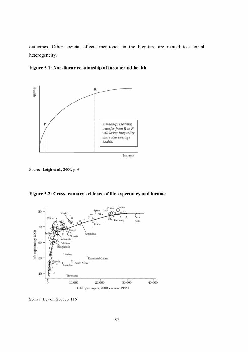
57

outcomes. Other societal effects mentioned in the literature are related to societal

heterogeneity.

Figure 5.1: Non-linear relationship of income and health

Source: Leigh et al., 2009, p. 6

Figure 5.2: Cross- country evidence of life expectancy and income

Source: Deaton, 2003, p. 116

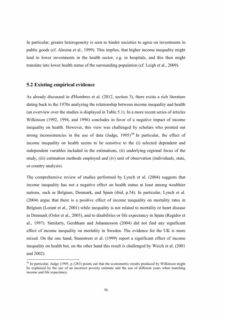
58

In particular, greater heterogeneity is seen to hinder societies to agree on investments in

public goods (cf. Alesina et al., 1999). This implies, that higher income inequality might

lead to lower investments in the health sector, e.g. in hospitals, and this then might

translate into lower health status of the surrounding population (cf. Leigh et al., 2009).

5.2 Existing empirical evidence

As already discussed in d'Hombres et al. (2012, section 3), there exists a rich literature

dating back to the 1970s analyzing the relationship between income inequality and health

(an overview over the studies is displayed in Table 5.1). In a more recent series of articles

Wilkinson (1992, 1994, and 1996) concludes in favor of a negative impact of income

inequality on health. However, this view was challenged by scholars who pointed out

strong inconsistencies in the use of data (Judge, 1995)26 In particular, the effect of

income inequality on health seems to be sensitive to the (i) selected dependent and

independent variables included in the estimations, (ii) underlying regional focus of the

study, (iii) estimation methods employed and (iv) unit of observation (individuals, state,

or country analysis).

The comprehensive review of studies performed by Lynch et al. (2004) suggests that

income inequality has not a negative effect on health status at least among wealthier

nations, such as Belgium, Denmark, and Spain (ibid, p.54). In particular, Lynch et al.

(2004) argue that there is a positive effect of income inequality on mortality rates in

Belgium (Lorant et al., 2001) while inequality is not related to mortality or heart disease

in Denmark (Osler et al., 2003), and to disabilities or life expectancy in Spain (Regidor et

al., 1997). Similarly, Gerdtham and Johannesson (2004) did not find any significant

effect of income inequality on mortality in Sweden. The evidence for the UK is more

mixed. On the one hand, Stanistreet et al. (1999) report a significant effect of income

inequality on health but, on the other hand this result is challenged by Weich et al. (2001

and 2002).

26 In particular, Judge (1995, p.1283) points out that the econometric results produced by Wilkinson might be explained by the use of an incorrect poverty estimate and the use of different years when matching income and life expectancy.

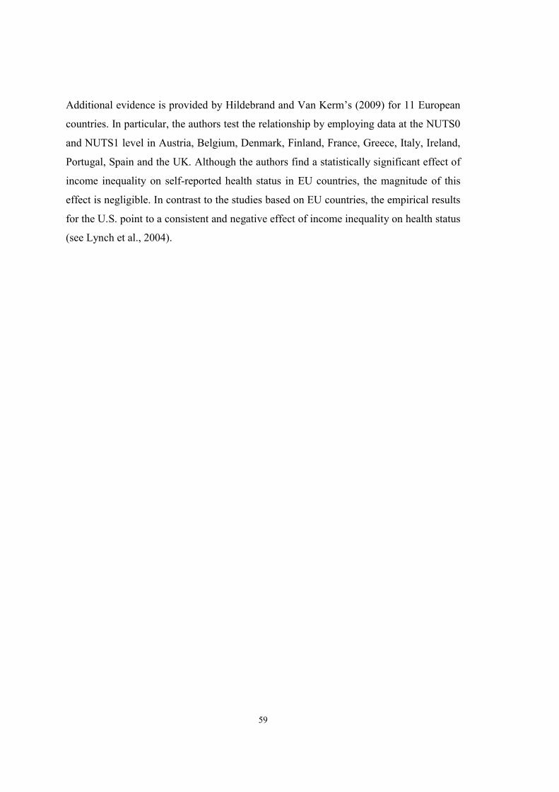
59

Additional evidence is provided by Hildebrand and Van Kerm’s (2009) for 11 European

countries. In particular, the authors test the relationship by employing data at the NUTS0

and NUTS1 level in Austria, Belgium, Denmark, Finland, France, Greece, Italy, Ireland,

Portugal, Spain and the UK. Although the authors find a statistically significant effect of

income inequality on self-reported health status in EU countries, the magnitude of this

effect is negligible. In contrast to the studies based on EU countries, the empirical results

for the U.S. point to a consistent and negative effect of income inequality on health status

(see Lynch et al., 2004).

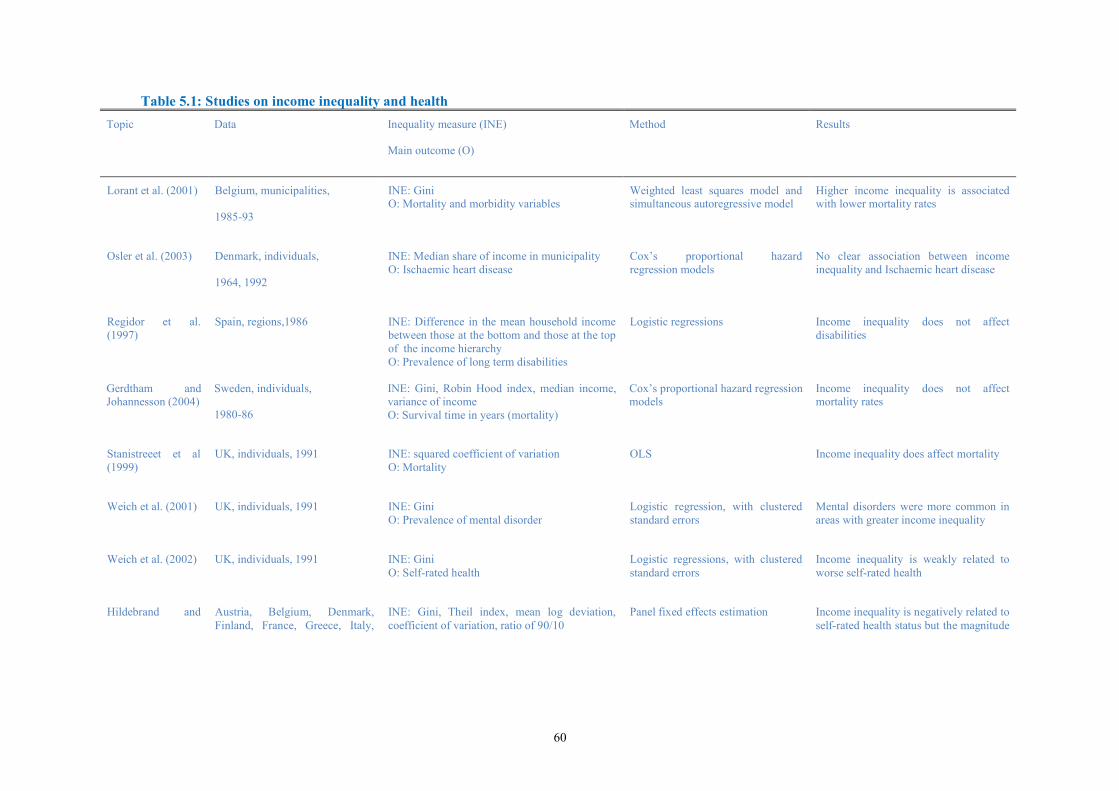
60

Table 5.1: Studies on income inequality and health

Topic Data Inequality measure (INE)

Main outcome (O)

Method Results

Lorant et al. (2001) Belgium, municipalities,

1985-93

INE: Gini O: Mortality and morbidity variables

Weighted least squares model and simultaneous autoregressive model

Higher income inequality is associated with lower mortality rates

Osler et al. (2003) Denmark, individuals,

1964, 1992

INE: Median share of income in municipality O: Ischaemic heart disease

Cox’s proportional hazard regression models

No clear association between income inequality and Ischaemic heart disease

Regidor et al. (1997)

Spain, regions,1986 INE: Difference in the mean household income between those at the bottom and those at the top of the income hierarchy O: Prevalence of long term disabilities

Logistic regressions Income inequality does not affect disabilities

Gerdtham and Johannesson (2004)

Sweden, individuals,

1980-86

INE: Gini, Robin Hood index, median income, variance of income O: Survival time in years (mortality)

Cox’s proportional hazard regression models

Income inequality does not affect mortality rates

Stanistreeet et al (1999)

UK, individuals, 1991 INE: squared coefficient of variation O: Mortality

OLS Income inequality does affect mortality

Weich et al. (2001) UK, individuals, 1991 INE: Gini O: Prevalence of mental disorder

Logistic regression, with clustered standard errors

Mental disorders were more common in areas with greater income inequality

Weich et al. (2002) UK, individuals, 1991 INE: Gini O: Self-rated health

Logistic regressions, with clustered standard errors

Income inequality is weakly related to worse self-rated health

Hildebrand and Austria, Belgium, Denmark, Finland, France, Greece, Italy,

INE: Gini, Theil index, mean log deviation, coefficient of variation, ratio of 90/10

Panel fixed effects estimation Income inequality is negatively related to self-rated health status but the magnitude

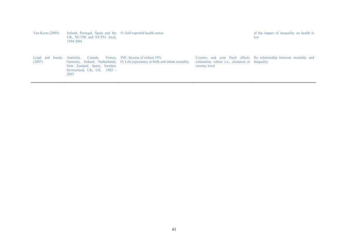
61

Van Kerm (2009) Ireland, Portugal, Spain and the UK, NUTS0 and NUTS1 level, 1994-2001

O: Self-reported health status of the impact of inequality on health is low

Leigh and Jencks (2007)

Australia, Canada, France, Germany, Ireland; Netherlands, New Zealand, Spain, Sweden, Switzerland, UK, US, 1903 - 2003

INE: Income of richest 10% O: Life expectancy at birth and infant mortality

Country and year fixed effects estimation, robust s.e., clustered at country level

No relationship between mortality and inequality

62

5.3 Empirical analysis

5.3.1 Health variables

While there are some cross-country studies (cf. Leigh and Jencks, 2006; and Judge et al., 1998) on

the effect of income inequality on health, more elaborated studies use individual-level data (see

Hildebrand and Van Kerm, 2009; Gerdtham and Johannesson, 2004; and Subramanian and

Kawachi, 2003). These analyses are able to distinguish between different mechanisms through

which income inequality might affect health. Hence, in a first step, we employ individual level

data from the EVS to analyze the effect of income inequality on self-reported health. In a second

step, we use country level data on life expectancy to estimate the effect of income inequality on a

country’s average level of health.

As already discussed in chapter 2, EVS is used to measure the social outcomes analyzed in this

study. In particular, to examine the effect of income inequality on health, we rely on self-reported

health information. More precisely, in the EVS, respondents are asked “All in all, how would you

describe your state of health these days? Would you say it is...”. Possible answers include very

good, good, fair, poor and very poor. For our baseline specification, the dependent health

indicator ranges from 1 to 5, with 1 measuring very poor health and 5 very good health.

Chart 5.1 displays the country average value of the population declaring to have good or very

good health. It is apparent that the level of people perceiving to be in a good health status varies

substantially across countries. In general, in most EU Member States over 50% of the population

reports good or very good health scores. Highest shares of individuals reporting good or very

good health, i.e. over 80%, are found in the Ireland, Denmark and Greece. Lowest levels of

citizens reporting good or very good health levels, i.e. below 50%, are observed in Lithuania,

Latvia, Estonia and Hungary.

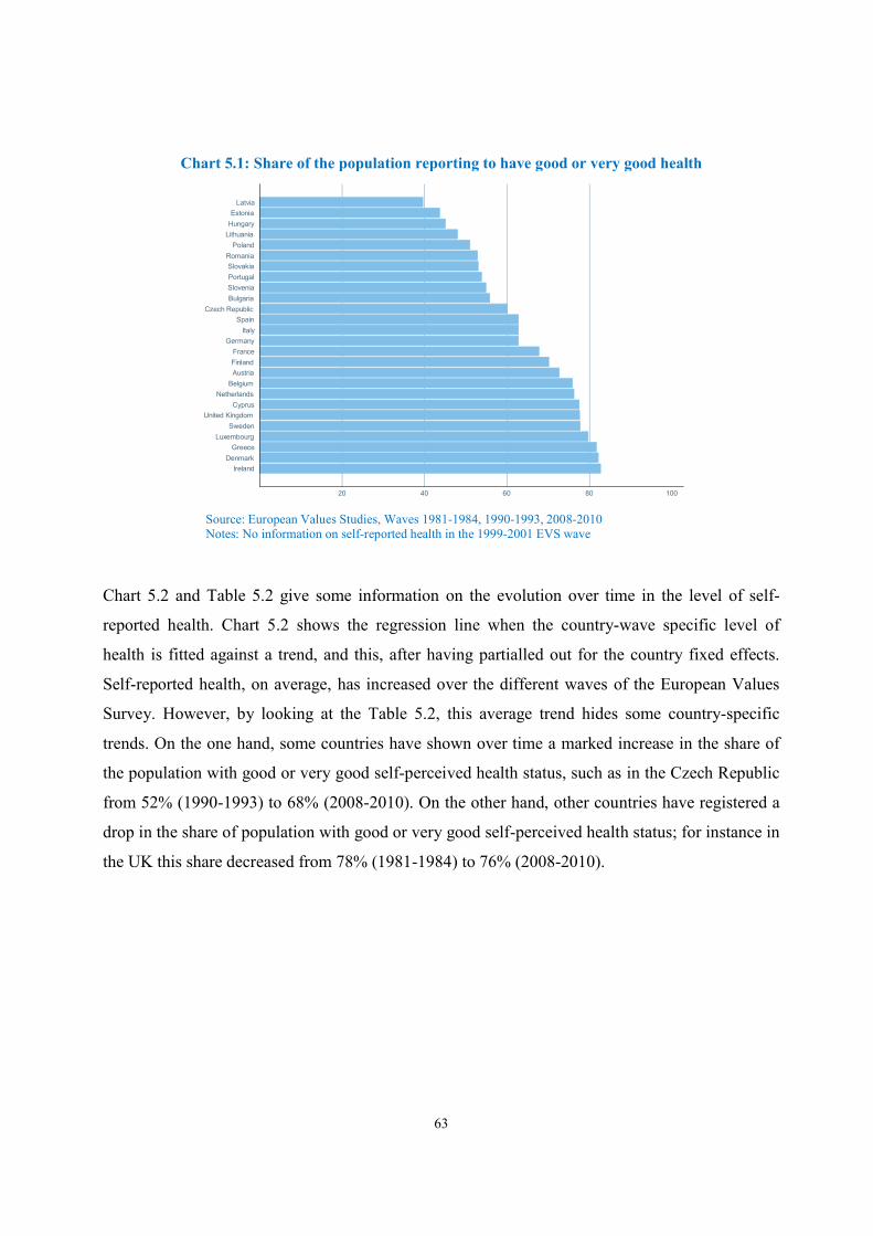
63

Chart 5.1: Share of the population reporting to have good or very good health

Source: European Values Studies, Waves 1981-1984, 1990-1993, 2008-2010 Notes: No information on self-reported health in the 1999-2001 EVS wave

Chart 5.2 and Table 5.2 give some information on the evolution over time in the level of self-

reported health. Chart 5.2 shows the regression line when the country-wave specific level of

health is fitted against a trend, and this, after having partialled out for the country fixed effects.

Self-reported health, on average, has increased over the different waves of the European Values

Survey. However, by looking at the Table 5.2, this average trend hides some country-specific

trends. On the one hand, some countries have shown over time a marked increase in the share of

the population with good or very good self-perceived health status, such as in the Czech Republic

from 52% (1990-1993) to 68% (2008-2010). On the other hand, other countries have registered a

drop in the share of population with good or very good self-perceived health status; for instance in

the UK this share decreased from 78% (1981-1984) to 76% (2008-2010).

20 40 60 80 100

Ireland

Denmark

Greece

Luxembourg

Sweden

United Kingdom

Cyprus

Netherlands

Belgium

Austria

Finland

France

Germany

Italy

Spain

Czech Republic

Bulgaria

Slovenia

Portugal

Slovakia

Romania

Poland

Lithuania

Hungary

Estonia

Latvia

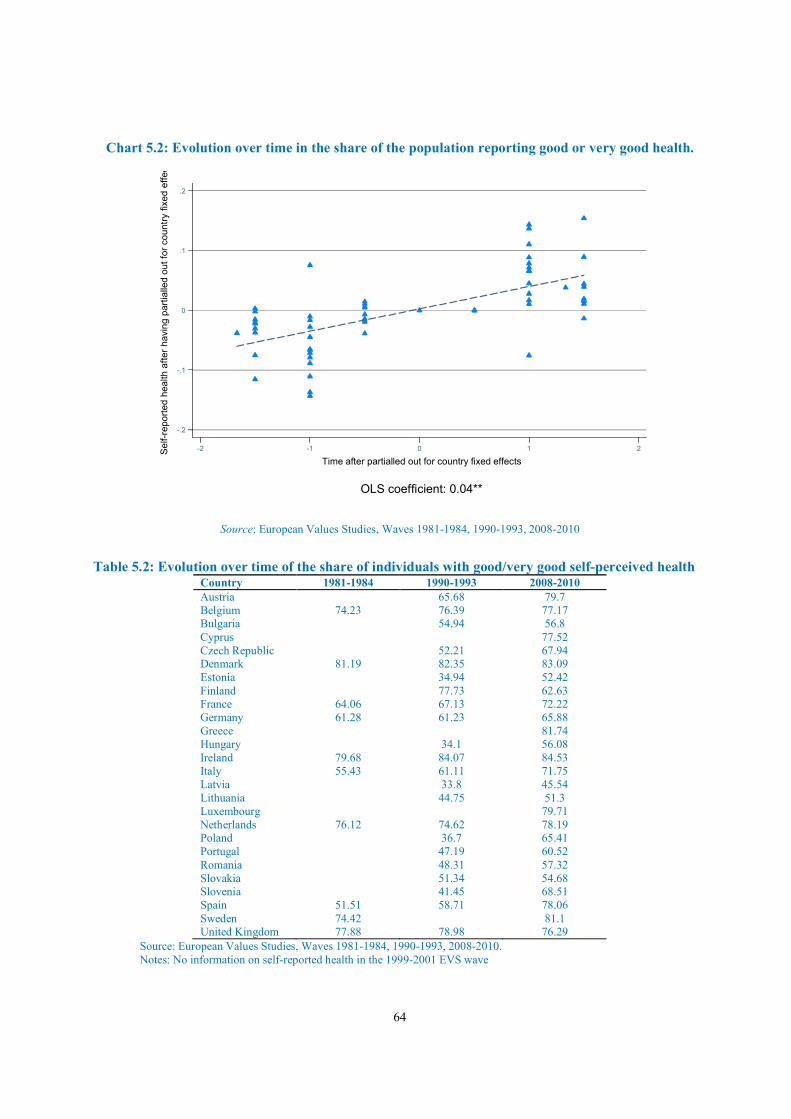
64

Chart 5.2: Evolution over time in the share of the population reporting good or very good health.

Source: European Values Studies, Waves 1981-1984, 1990-1993, 2008-2010

Table 5.2: Evolution over time of the share of individuals with good/very good self-perceived health Country 1981-1984 1990-1993 2008-2010 Austria 65.68 79.7 Belgium 74.23 76.39 77.17 Bulgaria 54.94 56.8 Cyprus 77.52 Czech Republic 52.21 67.94 Denmark 81.19 82.35 83.09 Estonia 34.94 52.42 Finland 77.73 62.63 France 64.06 67.13 72.22 Germany 61.28 61.23 65.88 Greece 81.74 Hungary 34.1 56.08 Ireland 79.68 84.07 84.53 Italy 55.43 61.11 71.75 Latvia 33.8 45.54 Lithuania 44.75 51.3 Luxembourg 79.71 Netherlands 76.12 74.62 78.19 Poland 36.7 65.41 Portugal 47.19 60.52 Romania 48.31 57.32 Slovakia 51.34 54.68 Slovenia 41.45 68.51 Spain 51.51 58.71 78.06 Sweden 74.42 81.1 United Kingdom 77.88 78.98 76.29

Source: European Values Studies, Waves 1981-1984, 1990-1993, 2008-2010. Notes: No information on self-reported health in the 1999-2001 EVS wave

-.2

-.1

0

.1

.2

Se

lf-r

ep

ort

ed

he

alth

aft

er

ha

vin

g p

art

ialle

d o

ut

for

co

un

try f

ixe

d e

ffe

cts

-2 -1 0 1 2

Time after partialled out for country fixed effects

OLS coefficient: 0.04**

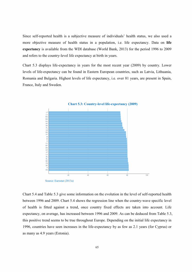
65

Since self-reported health is a subjective measure of individuals’ health status, we also used a

more objective measure of health status in a population, i.e. life expectancy. Data on life

expectancy is available from the WDI database (World Bank, 2013) for the period 1996 to 2009

and refers to the country-level life expectancy at birth in years.

Chart 5.3 displays life-expectancy in years for the most recent year (2009) by country. Lower

levels of life-expectancy can be found in Eastern European countries, such as Latvia, Lithuania,

Romania and Bulgaria. Highest levels of life expectancy, i.e. over 81 years, are present in Spain,

France, Italy and Sweden.

Chart 5.3: Country-level life-expectancy (2009)

Source: Eurostat (2013a)

Chart 5.4 and Table 5.3 give some information on the evolution in the level of self-reported health

between 1996 and 2009. Chart 5.4 shows the regression line when the country-wave specific level

of health is fitted against a trend, once country fixed effects are taken into account. Life

expectancy, on average, has increased between 1996 and 2009. As can be deduced from Table 5.3,

this positive trend seems to be true throughout Europe. Depending on the initial life expectancy in

1996, countries have seen increases in the life-expectancy by as few as 2.1 years (for Cyprus) or

as many as 4.9 years (Estonia).

20 40 60 80 100

ES

IT

SE

FR

BE

NL

EL

LU

AT

UK

DE

MT

CY

FI

IE

SI

PT

DK

CZ

PL

SK

EE

HU

BG

RO

LV

LT

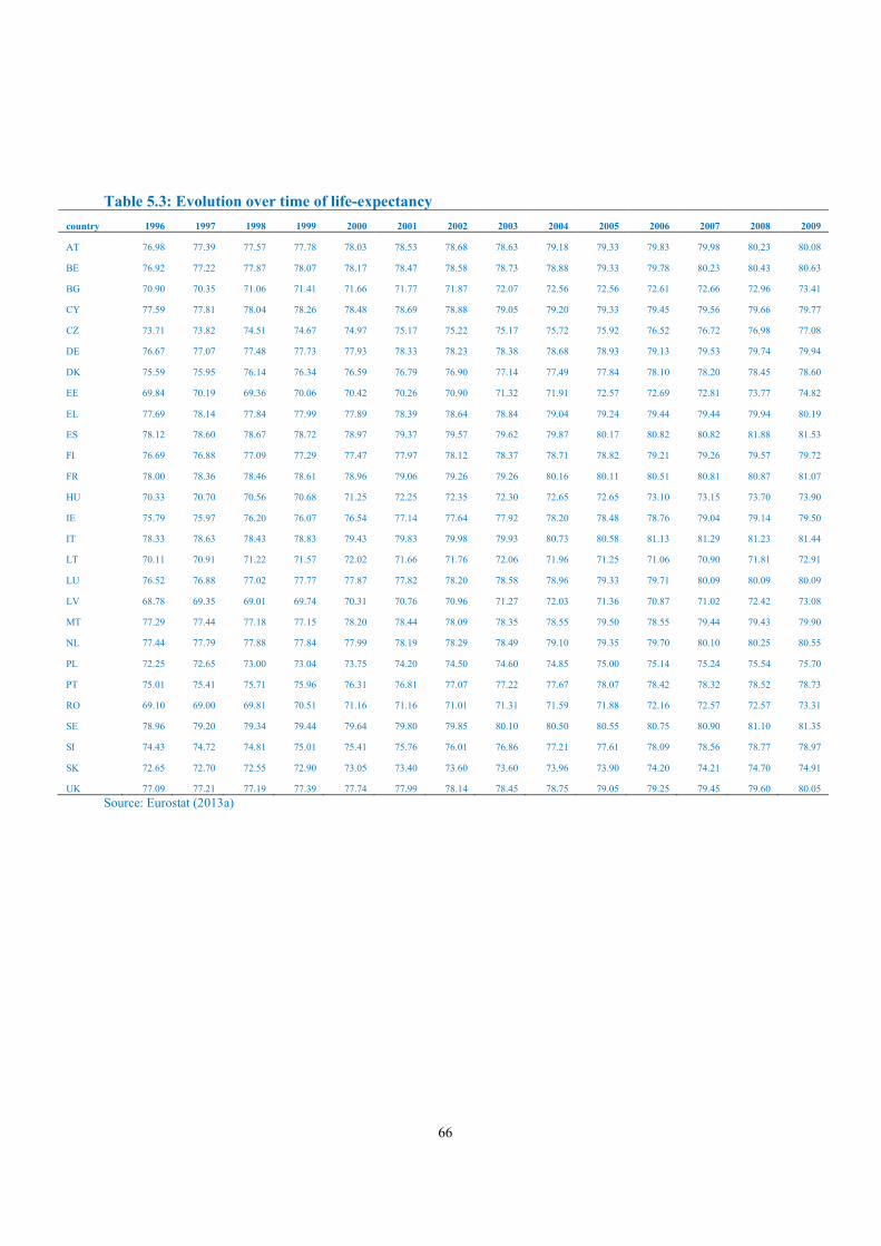
66

Table 5.3: Evolution over time of life-expectancy

country 1996 1997 1998 1999 2000 2001 2002 2003 2004 2005 2006 2007 2008 2009

AT 76.98 77.39 77.57 77.78 78.03 78.53 78.68 78.63 79.18 79.33 79.83 79.98 80.23 80.08

BE 76.92 77.22 77.87 78.07 78.17 78.47 78.58 78.73 78.88 79.33 79.78 80.23 80.43 80.63

BG 70.90 70.35 71.06 71.41 71.66 71.77 71.87 72.07 72.56 72.56 72.61 72.66 72.96 73.41

CY 77.59 77.81 78.04 78.26 78.48 78.69 78.88 79.05 79.20 79.33 79.45 79.56 79.66 79.77

CZ 73.71 73.82 74.51 74.67 74.97 75.17 75.22 75.17 75.72 75.92 76.52 76.72 76.98 77.08

DE 76.67 77.07 77.48 77.73 77.93 78.33 78.23 78.38 78.68 78.93 79.13 79.53 79.74 79.94

DK 75.59 75.95 76.14 76.34 76.59 76.79 76.90 77.14 77.49 77.84 78.10 78.20 78.45 78.60

EE 69.84 70.19 69.36 70.06 70.42 70.26 70.90 71.32 71.91 72.57 72.69 72.81 73.77 74.82

EL 77.69 78.14 77.84 77.99 77.89 78.39 78.64 78.84 79.04 79.24 79.44 79.44 79.94 80.19

ES 78.12 78.60 78.67 78.72 78.97 79.37 79.57 79.62 79.87 80.17 80.82 80.82 81.88 81.53

FI 76.69 76.88 77.09 77.29 77.47 77.97 78.12 78.37 78.71 78.82 79.21 79.26 79.57 79.72

FR 78.00 78.36 78.46 78.61 78.96 79.06 79.26 79.26 80.16 80.11 80.51 80.81 80.87 81.07

HU 70.33 70.70 70.56 70.68 71.25 72.25 72.35 72.30 72.65 72.65 73.10 73.15 73.70 73.90

IE 75.79 75.97 76.20 76.07 76.54 77.14 77.64 77.92 78.20 78.48 78.76 79.04 79.14 79.50

IT 78.33 78.63 78.43 78.83 79.43 79.83 79.98 79.93 80.73 80.58 81.13 81.29 81.23 81.44

LT 70.11 70.91 71.22 71.57 72.02 71.66 71.76 72.06 71.96 71.25 71.06 70.90 71.81 72.91

LU 76.52 76.88 77.02 77.77 77.87 77.82 78.20 78.58 78.96 79.33 79.71 80.09 80.09 80.09

LV 68.78 69.35 69.01 69.74 70.31 70.76 70.96 71.27 72.03 71.36 70.87 71.02 72.42 73.08

MT 77.29 77.44 77.18 77.15 78.20 78.44 78.09 78.35 78.55 79.50 78.55 79.44 79.43 79.90

NL 77.44 77.79 77.88 77.84 77.99 78.19 78.29 78.49 79.10 79.35 79.70 80.10 80.25 80.55

PL 72.25 72.65 73.00 73.04 73.75 74.20 74.50 74.60 74.85 75.00 75.14 75.24 75.54 75.70

PT 75.01 75.41 75.71 75.96 76.31 76.81 77.07 77.22 77.67 78.07 78.42 78.32 78.52 78.73

RO 69.10 69.00 69.81 70.51 71.16 71.16 71.01 71.31 71.59 71.88 72.16 72.57 72.57 73.31

SE 78.96 79.20 79.34 79.44 79.64 79.80 79.85 80.10 80.50 80.55 80.75 80.90 81.10 81.35

SI 74.43 74.72 74.81 75.01 75.41 75.76 76.01 76.86 77.21 77.61 78.09 78.56 78.77 78.97

SK 72.65 72.70 72.55 72.90 73.05 73.40 73.60 73.60 73.96 73.90 74.20 74.21 74.70 74.91

UK 77.09 77.21 77.19 77.39 77.74 77.99 78.14 78.45 78.75 79.05 79.25 79.45 79.60 80.05

Source: Eurostat (2013a)

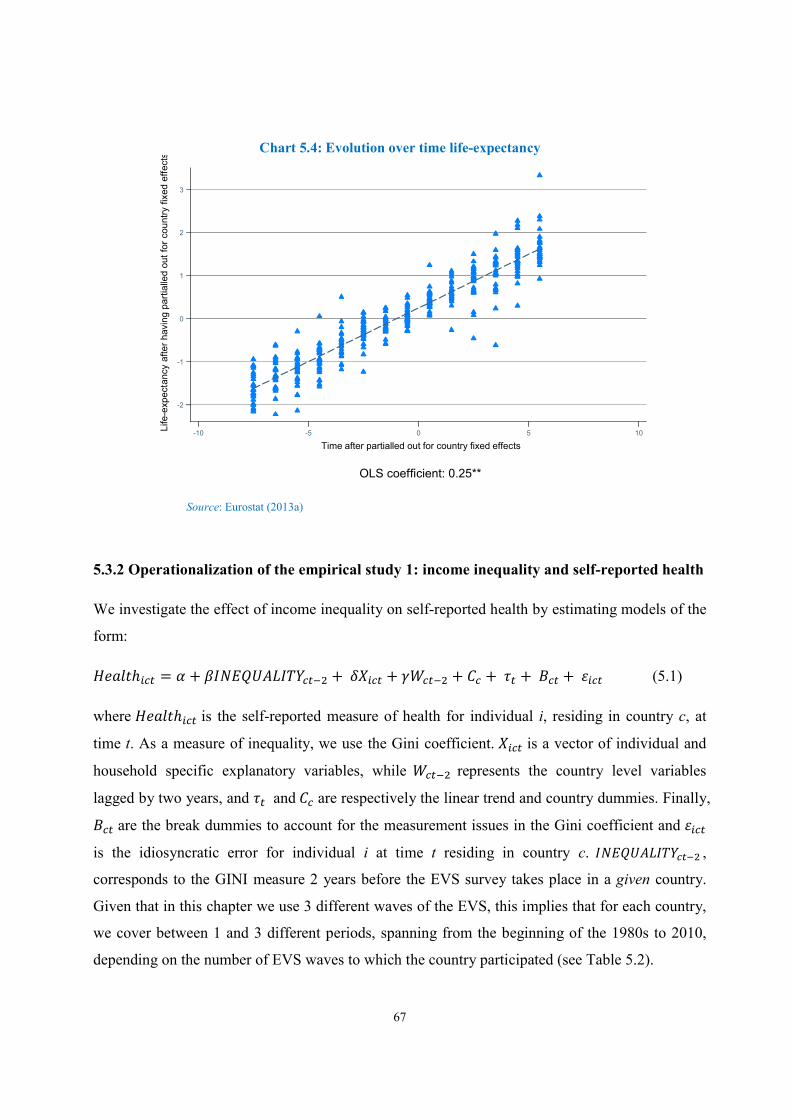
67

Chart 5.4: Evolution over time life-expectancy

Source: Eurostat (2013a)

5.3.2 Operationalization of the empirical study 1: income inequality and self-reported health

We investigate the effect of income inequality on self-reported health by estimating models of the

form:

�����ℎ��� = � + ��������������� +����� + ������ + �� +��+��� + ���� (5.1)

where �����ℎ��� is the self-reported measure of health for individual i, residing in country c, at

time t. As a measure of inequality, we use the Gini coefficient. ���� is a vector of individual and

household specific explanatory variables, while ����� represents the country level variables

lagged by two years, and �� and�� are respectively the linear trend and country dummies. Finally,

��� are the break dummies to account for the measurement issues in the Gini coefficient and ����

is the idiosyncratic error for individual i at time t residing in country c. �������������� ,

corresponds to the GINI measure 2 years before the EVS survey takes place in a given country.

Given that in this chapter we use 3 different waves of the EVS, this implies that for each country,

we cover between 1 and 3 different periods, spanning from the beginning of the 1980s to 2010,

depending on the number of EVS waves to which the country participated (see Table 5.2).

-2

-1

0

1

2

3

Life

-exp

ecta

ncy a

fte

r h

avin

g p

art

ialle

d o

ut

for

co

un

try f

ixe

d e

ffe

cts

-10 -5 0 5 10

Time after partialled out for country fixed effects

OLS coefficient: 0.25**

68

The reason for including a lagged Gini variable and lagged country level variable is as follows.

Including a lagged structure of the variable allows us to account for delayed effects of the

explanatory variables on health and to reduce the potential bias driven by reverse causation.

However, the scholarly debate did not reach a consensus yet on which time lag is most appropriate

to use when studying the effect of inequality on health. The appropriate lag structure hinges on the

mechanism underlying the association between income inequality and health. For example rising

income inequality might harm an individual’s health outcome in the long-run through its effect on

increasing the stress of managing professional and personal life. On the contrary, if income

inequality exacerbates crime and homicide rates then the effect on health can occur in the short-

run (Leigh and Jencks, 2007). To check the robustness of our analysis, we also report results when

using the contemporaneous Gini variable as well as the 3 year lag (see Table 5.5 and Table 5.8).

We test the validity of the absolute income hypothesis, i.e. an individual’s absolute income affects

health status, by including in ���� a measure of an individual’s income. In addition we include a

conventionally used set of covariates to account for individual level characteristics, i.e. age, sex,

educational background, information on occupational status, marital status, being religious, and

number of children (Hildebrand and Van Kerm, 2009; Gerdtham and Johannesson, 2004; and

Mellor and Milyo, 2002).27

In the present analysis we also account for some important country-specific characteristics related

to the country health system. In particular, it is reasonable to assume that a population’s health

status might depend on health expenditure. Data on a country’s total health expenditure per capita

in Dollar PPP is available from the OECD (2012). For convenience we transform the variable in

logarithmic form and denote it by health expenditure. As additional country level variables

�����, we consider the age distribution in the population by using the variable dependents. This

variable measures the proportion of people aged 0-15 and 65+ over the 15-64 year-old population.

Last, we include a measure for the population size per country, i.e. population. The information on

population is transformed in lognormal form. A precise description of all individual level and

country level variables can be found in Table 5.4. In addition, correlations between individual

27 Beyond these important individual characteristics, scholars have also included control variables on ethnic identity, health care coverage and health behavior, such as exercise, diet, and smoking behavior, in their estimations (Mellor and Milyo, 2002). Due to data limitation of the EVS, we are however neither able to account for the origin of the individual nor for his health behavior.

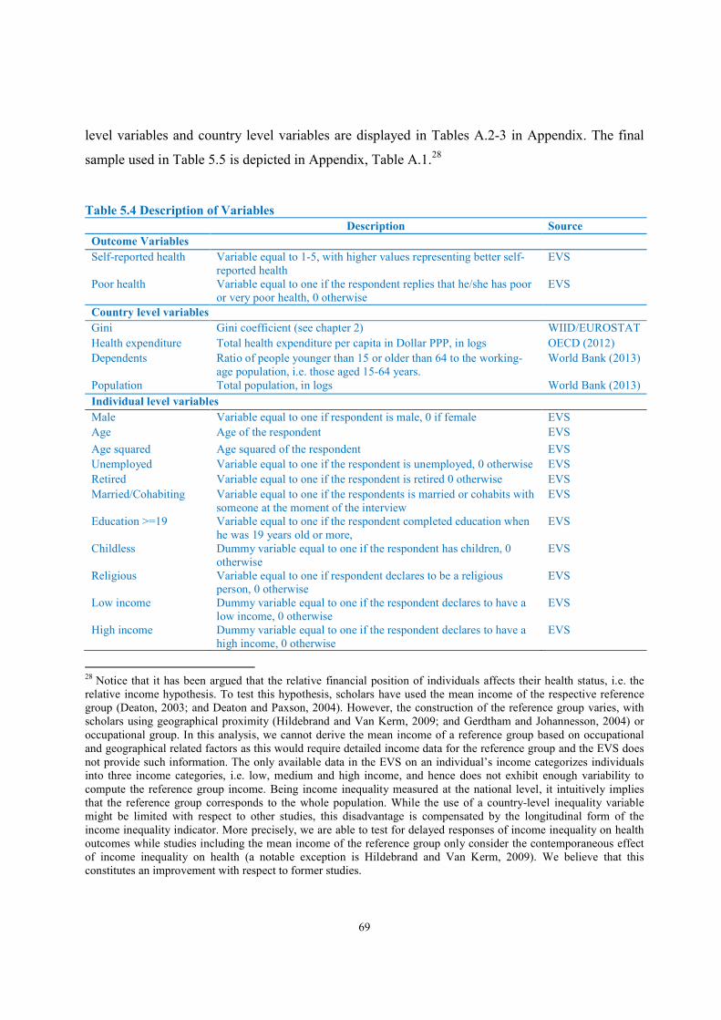
69

level variables and country level variables are displayed in Tables A.2-3 in Appendix. The final

sample used in Table 5.5 is depicted in Appendix, Table A.1.28

Table 5.4 Description of Variables

Description Source

Outcome Variables

Self-reported health Variable equal to 1-5, with higher values representing better self-reported health

EVS

Poor health Variable equal to one if the respondent replies that he/she has poor or very poor health, 0 otherwise

EVS

Country level variables

Gini Gini coefficient (see chapter 2) WIID/EUROSTAT

Health expenditure Total health expenditure per capita in Dollar PPP, in logs OECD (2012)

Dependents Ratio of people younger than 15 or older than 64 to the working-age population, i.e. those aged 15-64 years.

World Bank (2013)

Population Total population, in logs World Bank (2013)

Individual level variables

Male Variable equal to one if respondent is male, 0 if female EVS

Age Age of the respondent EVS

Age squared Age squared of the respondent EVS

Unemployed Variable equal to one if the respondent is unemployed, 0 otherwise EVS

Retired Variable equal to one if the respondent is retired 0 otherwise EVS

Married/Cohabiting Variable equal to one if the respondents is married or cohabits with someone at the moment of the interview

EVS

Education >=19 Variable equal to one if the respondent completed education when he was 19 years old or more,

EVS

Childless Dummy variable equal to one if the respondent has children, 0 otherwise

EVS

Religious Variable equal to one if respondent declares to be a religious person, 0 otherwise

EVS

Low income Dummy variable equal to one if the respondent declares to have a low income, 0 otherwise

EVS

High income Dummy variable equal to one if the respondent declares to have a high income, 0 otherwise

EVS

28 Notice that it has been argued that the relative financial position of individuals affects their health status, i.e. the relative income hypothesis. To test this hypothesis, scholars have used the mean income of the respective reference group (Deaton, 2003; and Deaton and Paxson, 2004). However, the construction of the reference group varies, with scholars using geographical proximity (Hildebrand and Van Kerm, 2009; and Gerdtham and Johannesson, 2004) or occupational group. In this analysis, we cannot derive the mean income of a reference group based on occupational and geographical related factors as this would require detailed income data for the reference group and the EVS does not provide such information. The only available data in the EVS on an individual’s income categorizes individuals into three income categories, i.e. low, medium and high income, and hence does not exhibit enough variability to compute the reference group income. Being income inequality measured at the national level, it intuitively implies that the reference group corresponds to the whole population. While the use of a country-level inequality variable might be limited with respect to other studies, this disadvantage is compensated by the longitudinal form of the income inequality indicator. More precisely, we are able to test for delayed responses of income inequality on health outcomes while studies including the mean income of the reference group only consider the contemporaneous effect of income inequality on health (a notable exception is Hildebrand and Van Kerm, 2009). We believe that this constitutes an improvement with respect to former studies.

70

Note: Wave, break and country dummies are also included in all estimates.

5.3.3 Econometric results 1: income inequality and self-reported health

Estimation results for the effect of income inequality on self-reported health are displayed in

Table 5.5. Linear regressions are used for estimating models 1-5. We start with a baseline

estimation, which only includes the Gini variable as the main explanatory variable, as well as a

linear trend, break dummies and country dummies. This model is presented in column 1 of Table

5.5. Column 2 includes individual-level variables, while column 3 also considers macroeconomics

variables. In addition, a series of robustness checks are reported in columns 4-7. In particular, we

re-estimate model 3 by using the contemporaneous Gini variable and the 3 year lag of the Gini

coefficient instead of the 2 year lag (columns 4 and 5 respectively). Next, we check whether our

results are robust to a different operationalization of the dependent variable. While in the

estimations 1-5 we employ the 5-score health variable, estimation results in columns 6-7, the

dependent variable is a binary variable which is equal to 1 if respondents declare to have very

poor or poor health and 0 otherwise. In these cases, we apply a maximum likelihood estimator

which account for the nonlinear relationship between the dependent and explanatory variables,

namely the probit model. A two-year and a three-year lag are used in models 6 and 7 respectively.

Note that Huber-White standard errors clustered at the country level are used throughout the

aforementioned estimations. These standard errors are robust to arbitrary forms of error

correlation within a country.

The most important conclusion reached from the estimation results presented in Table 5.5 is that

once we control for individual and macroeconomic variables, in none of the regressions does the

Gini coefficient turn significant. This suggests that income inequality is not significantly related to

self-reported health. This result holds irrespective of the lag structure used for the Gini index, i.e.

no lag, 2 and 3 year lag, and the hypothesized functional form of the model.

On the other hand, the individual level variables are significantly different from zero and with the

expected sign. In particular, older individuals have a lower self-reported health status (or a higher

probability of having reported very poor or poor health, in estimations 6 and 7) and the negative

effect of age decreases with increasing age (as can be seen by the significant age squared variable).

Moreover, men have a higher self-reported health status (or lower probability for poor health). In

71

addition, more educated people have higher levels of self-reported health (or lower probability for

poor health). For individuals who are either unemployed or retired the estimation results suggest

that health statuses are lower compared to the omitted group (employed). Next, we find that our

results support the absolute income hypothesis, i.e. a significant effect of individual income on

self-reported health. In particular, compared to medium income (i.e. the omitted category),

individual with low income are associated with lower self-reported health, whereas high income

earners exhibit better self-reported health outcomes. Being a religious person does not affect self-

reported health when measured on a 1-5 scale, but turns significantly positive for the binary

dependent variable. In addition, there seems to be a positive effect of being in a stable partnership

and having children. In particular, individuals who are either married or cohabitate and/or have

children seem to have higher levels of health (or lower probability of having poor health).

Now turning to the country-level variables, our estimations suggest that there might be a

significant relationship between public health expenditure and self-reported health. More precisely,

when using a three year lag, higher spending on health seems to increase self-reported health (and

decrease the probability of having poor health, see columns 4 and 6). In addition, the size of the

population is negative and significant. Last, the dependency ratio remains largely insignificant

throughout the estimations. Note that a further robustness check, where population is excluded

from the estimation is reported in Table A.4 in the Appendix.29

29 In contrast to estimations on happiness and social capital we do not include GDP per capita in the estimations on self-reported health, since GDP per capita is highly correlated with health expenditure (correlation coefficient = 0.82) and when both variables are included in the estimation their coefficients cannot be estimated precisely, i.e. they both turn insignificant. However, the coefficient of the Gini coefficient remains unchanged to the inclusion of GDP per capita in the estimation (results not shown).

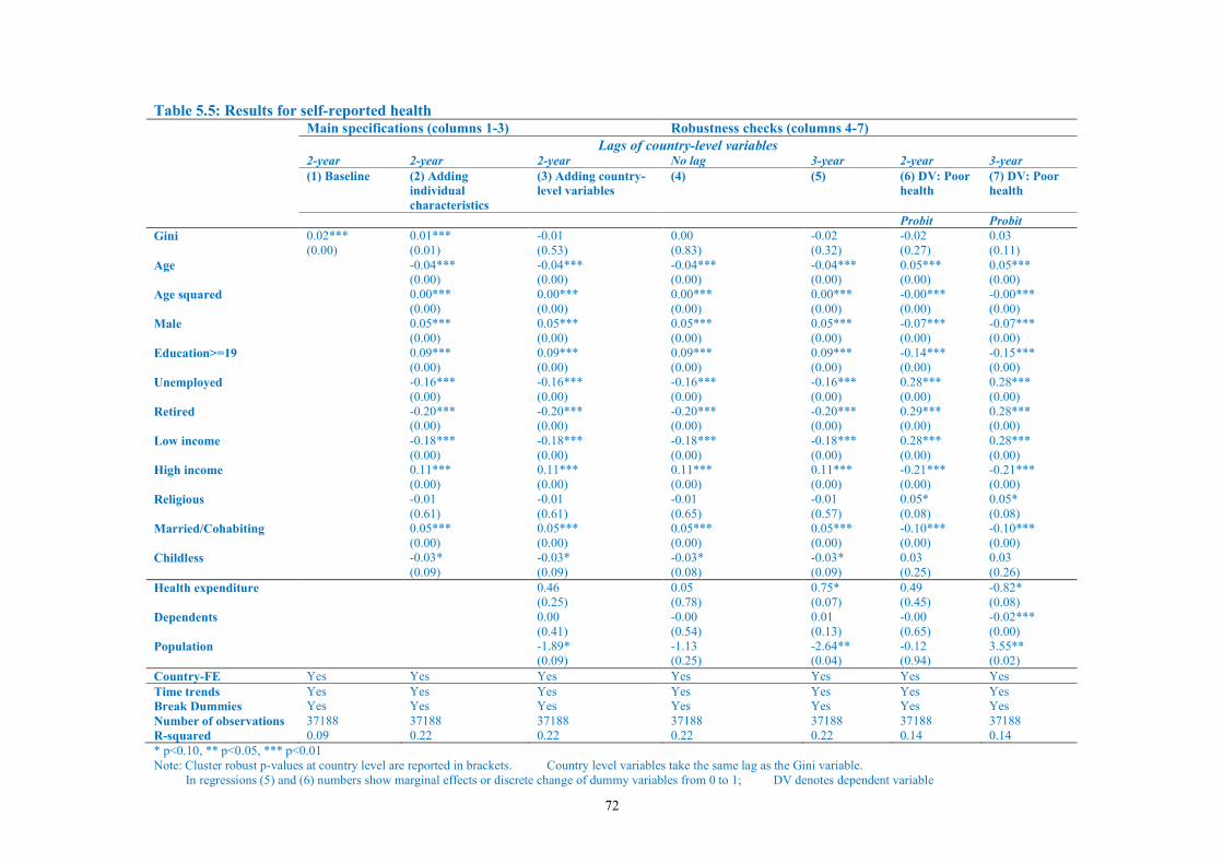
72

Table 5.5: Results for self-reported health Main specifications (columns 1-3) Robustness checks (columns 4-7) Lags of country-level variables 2-year 2-year 2-year No lag 3-year 2-year 3-year (1) Baseline (2) Adding

individual characteristics

(3) Adding country-level variables

(4) (5) (6) DV: Poor health

(7) DV: Poor health

Probit Probit Gini 0.02*** 0.01*** -0.01 0.00 -0.02 -0.02 0.03 (0.00) (0.01) (0.53) (0.83) (0.32) (0.27) (0.11) Age -0.04*** -0.04*** -0.04*** -0.04*** 0.05*** 0.05*** (0.00) (0.00) (0.00) (0.00) (0.00) (0.00) Age squared 0.00*** 0.00*** 0.00*** 0.00*** -0.00*** -0.00*** (0.00) (0.00) (0.00) (0.00) (0.00) (0.00) Male 0.05*** 0.05*** 0.05*** 0.05*** -0.07*** -0.07*** (0.00) (0.00) (0.00) (0.00) (0.00) (0.00) Education>=19 0.09*** 0.09*** 0.09*** 0.09*** -0.14*** -0.15*** (0.00) (0.00) (0.00) (0.00) (0.00) (0.00) Unemployed -0.16*** -0.16*** -0.16*** -0.16*** 0.28*** 0.28*** (0.00) (0.00) (0.00) (0.00) (0.00) (0.00) Retired -0.20*** -0.20*** -0.20*** -0.20*** 0.29*** 0.28*** (0.00) (0.00) (0.00) (0.00) (0.00) (0.00) Low income -0.18*** -0.18*** -0.18*** -0.18*** 0.28*** 0.28*** (0.00) (0.00) (0.00) (0.00) (0.00) (0.00) High income 0.11*** 0.11*** 0.11*** 0.11*** -0.21*** -0.21*** (0.00) (0.00) (0.00) (0.00) (0.00) (0.00) Religious -0.01 -0.01 -0.01 -0.01 0.05* 0.05* (0.61) (0.61) (0.65) (0.57) (0.08) (0.08) Married/Cohabiting 0.05*** 0.05*** 0.05*** 0.05*** -0.10*** -0.10*** (0.00) (0.00) (0.00) (0.00) (0.00) (0.00) Childless -0.03* -0.03* -0.03* -0.03* 0.03 0.03 (0.09) (0.09) (0.08) (0.09) (0.25) (0.26) Health expenditure 0.46 0.05 0.75* 0.49 -0.82* (0.25) (0.78) (0.07) (0.45) (0.08) Dependents 0.00 -0.00 0.01 -0.00 -0.02*** (0.41) (0.54) (0.13) (0.65) (0.00) Population -1.89* -1.13 -2.64** -0.12 3.55** (0.09) (0.25) (0.04) (0.94) (0.02) Country-FE Yes Yes Yes Yes Yes Yes Yes Time trends Yes Yes Yes Yes Yes Yes Yes Break Dummies Yes Yes Yes Yes Yes Yes Yes Number of observations 37188 37188 37188 37188 37188 37188 37188 R-squared 0.09 0.22 0.22 0.22 0.22 0.14 0.14 * p<0.10, ** p<0.05, *** p<0.01 Note: Cluster robust p-values at country level are reported in brackets. Country level variables take the same lag as the Gini variable. In regressions (5) and (6) numbers show marginal effects or discrete change of dummy variables from 0 to 1; DV denotes dependent variable

73

5.3.4 Operationalization of the empirical study 2: income inequality and life expectancy

In contrast to the estimation of self-reported health of individuals, the study of life

expectancy is operationalized at the country level and estimated as follows:

���������������� = � + ��������������� + ������+�� + ��� (5.2)

where ���������������� is the life expectancy in years for a country c, at time t. As a

measure of inequality we use the Gini coefficient as well as the S80/S20 indicator, both

drawn from Eurostat (2013a). As for the analysis on self-reported health, income inequality

enters equation (5.2) with a two years lag. Furthermore, we include country level variables

lagged 2 years (W����) and country fixed effects �� in order to control for all time-invariant

country heterogeneity. As for the other social outcomes, some robustness checks will be

carried out to check the sensitivity of the findings to the assumptions underlying the model

specification.

Note that in this estimation we do not include break dummies. This is due to the fact that the

period covered is shorter (i.e. running from 1996 to 2006) than the one employed in the

empirical analysis on the determinants of self-reported health. For the recent period, we can

rely on consistent Gini and S80/S20 measures, readily available from Eurostat. Hence, we do

not need to account for any breaks in the construction of the Gini variable.

As for the individual level analysis, to estimate the effect of income inequality on life

expectancy it is necessary to control for other confounding factors. In the following we

describe the explanatory variables used in the present exercise.

According to the absolute income hypothesis more wealthy countries are expected to attain

higher health status than comparably poorer countries. To proxy a country’s income, we use

the log of GDP per capita measured in constant 2005 international dollars (PPP). We also

include a measure of a country’s expenditure on health. Data on a country’s total health

expenditure per capita in dollar PPP is available from the OECD (2012). The variable enters

equation (5.2) in logarithmic form.

In addition, we make use of a wide range of additional variables to control for a country’s

economic and socio-demographic characteristics. In particular, we include an indicator of the

educational level of the population in the country (gross school enrollment rate in tertiary

education), an indicator of the female labor market participation (percentage of active women

74

aged 20-64), the age dependency ratio (proportion of people aged 0-15 and 65+ over the 15-

64 year-old population), and a measure for the population size. A description of the variables

included as well as their label can be found in Table 5.6.

Table 5.6: Description of Variables Description Source

Outcome Variables

Life expectancy Country-level variable on life-expectancy at birth, total (years) World Bank (2013)

Country level control variables

Gini Gini coefficient of equivalised disposable income Eurostat (2013a)

S80/S20 S80/S20 income quintile share ratio Eurostat (2013a)

GDP GDP per capita in constant 2005 Intl. Dollar (PPP), in logs World Bank (2013)

Health expenditure Total health expenditure per capita in Dollar PPP, in logs OECD (2012)

Tertiary education Gross tertiary school enrollment in percent World Bank (2013)

Female work Percentage of women age 20-64 years that are active in the labor market

Eurostat (2013a)

Dependents Ratio of people younger than 15 or older than 64 to the working-age population, i.e. those aged 15-64 years.

World Bank (2013)

Population Total population, in logs World Bank (2013)

Looking at the correlation matrix displayed in Table 5.7, we see that there are a number of

high correlations between control variables, which might lead to distorted econometric

findings. In particular, health expenditure and GDP are highly correlated (0.88). In addition,

tertiary education is highly correlated with health expenditure (0.75) as well as correlated

with GDP (0.4) and with the dependency ratio (0.4). Last, the dependency ratio is highly

correlated with health expenditure (0.58). These high correlations suggest that the

coefficients of the aforementioned variables might not be estimated precisely. Hence various

robustness checks were carried out to ensure that the results for the Gini variable are not

driven by multicollinearity issues (see Table 5.8 and Appendix, Table A.5).

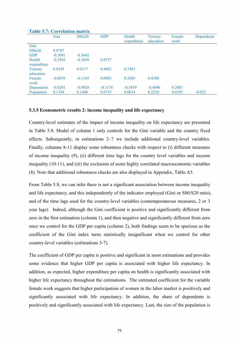
75

Table 5.7: Correlation matrix Gini S80s20 GDP Health

expenditure Tertiary education

Female work

Dependents

Gini S80s20 0.9707 GDP -0.3091 -0.3642 Health expenditure

-0.2945 -0.3656 0.8737

Tertiary education

0.0349 0.0117 0.4082 0.7483

Female work

-0.0676 -0.1345 0.0085 0.2885 0.4380

Dependents -0.0291 -0.0928 -0.1176 -0.5859 -0.4096 0.2083 Population 0.1354 0.1448 0.0733 0.0014 0.2210 0.0385 -0.022

5.3.5 Econometric results 2: income inequality and life expectancy

Country-level estimates of the impact of income inequality on life expectancy are presented

in Table 5.8. Model of column 1 only controls for the Gini variable and the country fixed

effects. Subsequently, in estimations 2–7 we include additional country-level variables.

Finally, columns 8-11 display some robustness checks with respect to (i) different measures

of income inequality (9), (ii) different time lags for the country level variables and income

inequality (10-11), and (iii) the exclusion of some highly correlated macroeconomic variables

(8). Note that additional robustness checks are also displayed in Appendix, Table A5.

From Table 5.8, we can infer there is not a significant association between income inequality

and life expectancy, and this independently of the indicator employed (Gini or S80/S20 ratio),

and of the time lags used for the country-level variables (contemporaneous measures, 2 or 3

year lags). Indeed, although the Gini coefficient is positive and significantly different from

zero in the first estimation (column 1), and then negative and significantly different from zero

once we control for the GDP per capita (column 2), both findings seem to be spurious as the

coefficient of the Gini index turns statistically insignificant when we control for other

country-level variables (estimations 3-7).

The coefficient of GDP per capita is positive and significant in most estimations and provides

some evidence that higher GDP per capita is associated with higher life expectancy. In

addition, as expected, higher expenditure per capita on health is significantly associated with

higher life expectancy throughout the estimations. The estimated coefficient for the variable

female work suggests that higher participation of women in the labor market is positively and

significantly associated with life expectancy. In addition, the share of dependents is

positively and significantly associated with life expectancy. Last, the size of the population is

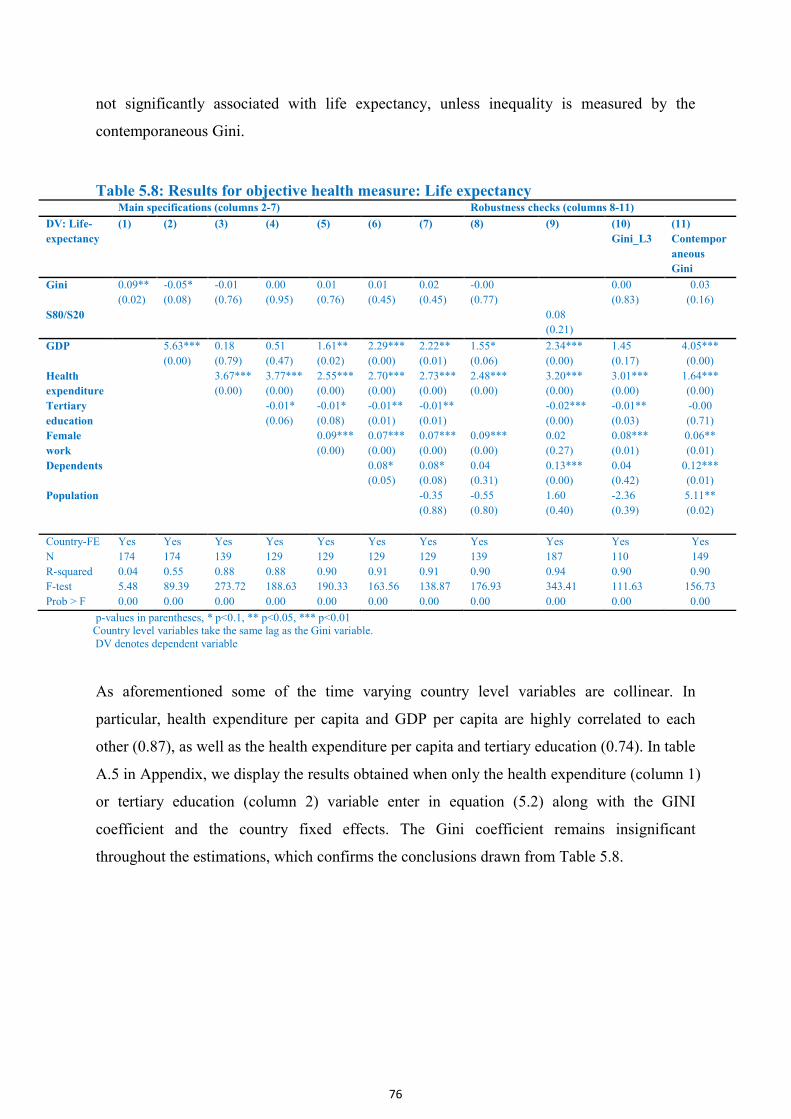
76

not significantly associated with life expectancy, unless inequality is measured by the

contemporaneous Gini.

Table 5.8: Results for objective health measure: Life expectancy Main specifications (columns 2-7) Robustness checks (columns 8-11)

DV: Life-

expectancy

(1) (2) (3) (4) (5) (6) (7) (8) (9) (10)

Gini_L3

(11)

Contempor

aneous

Gini

Gini 0.09** -0.05* -0.01 0.00 0.01 0.01 0.02 -0.00 0.00 0.03

(0.02) (0.08) (0.76) (0.95) (0.76) (0.45) (0.45) (0.77) (0.83) (0.16)

S80/S20 0.08

(0.21)

GDP 5.63*** 0.18 0.51 1.61** 2.29*** 2.22** 1.55* 2.34*** 1.45 4.05***

(0.00) (0.79) (0.47) (0.02) (0.00) (0.01) (0.06) (0.00) (0.17) (0.00)

Health 3.67*** 3.77*** 2.55*** 2.70*** 2.73*** 2.48*** 3.20*** 3.01*** 1.64***

expenditure (0.00) (0.00) (0.00) (0.00) (0.00) (0.00) (0.00) (0.00) (0.00)

Tertiary -0.01* -0.01* -0.01** -0.01** -0.02*** -0.01** -0.00

education (0.06) (0.08) (0.01) (0.01) (0.00) (0.03) (0.71)

Female 0.09*** 0.07*** 0.07*** 0.09*** 0.02 0.08*** 0.06**

work (0.00) (0.00) (0.00) (0.00) (0.27) (0.01) (0.01)

Dependents 0.08* 0.08* 0.04 0.13*** 0.04 0.12***

(0.05) (0.08) (0.31) (0.00) (0.42) (0.01)

Population -0.35 -0.55 1.60 -2.36 5.11**

(0.88) (0.80) (0.40) (0.39) (0.02)

Country-FE Yes Yes Yes Yes Yes Yes Yes Yes Yes Yes Yes

N 174 174 139 129 129 129 129 139 187 110 149

R-squared 0.04 0.55 0.88 0.88 0.90 0.91 0.91 0.90 0.94 0.90 0.90

F-test 5.48 89.39 273.72 188.63 190.33 163.56 138.87 176.93 343.41 111.63 156.73

Prob > F 0.00 0.00 0.00 0.00 0.00 0.00 0.00 0.00 0.00 0.00 0.00

p-values in parentheses, * p<0.1, ** p<0.05, *** p<0.01 Country level variables take the same lag as the Gini variable. DV denotes dependent variable

As aforementioned some of the time varying country level variables are collinear. In

particular, health expenditure per capita and GDP per capita are highly correlated to each

other (0.87), as well as the health expenditure per capita and tertiary education (0.74). In table

A.5 in Appendix, we display the results obtained when only the health expenditure (column 1)

or tertiary education (column 2) variable enter in equation (5.2) along with the GINI

coefficient and the country fixed effects. The Gini coefficient remains insignificant

throughout the estimations, which confirms the conclusions drawn from Table 5.8.

77

6. Conclusion

This report constitutes the third deliverable of a comprehensive series of studies initiated by

the European Commission on the social and economic challenges associated with rising

income inequalities. The present study provides a multivariate analysis of the effect of

income inequality on three important social outcomes, i.e. health, social capital, and

happiness. To arrive at a robust estimation of the effect of income inequality on these social

outcomes, we have taken great care to construct a dataset that covers the greatest number of

the EU member states and covers the longest possible time period. In addition, we employ a

wide number of individual- and country-level control variables, and include a variety of

robustness checks in our empirical estimations.

Our study suggests that the adverse effect of income inequality on a plurality of societal

development challenges as proposed by Wilkinson and Pickett (2009) cannot be confirmed

by the data, with the important exception of trust. In particular, our analysis cannot

confirm the hypothesis of a strong and significant effect of income inequality on health,

happiness and participation in associational activities. The result of no-effect of income

inequality is robust to the inclusion of a large number of individual- and country-specific

variables, different time lags of the inequality variable and different functional forms of the

dependent variables. We believe that Wilkinson and Pickett’s (2009) findings are largely

driven by the omission of relevant country characteristics that are simultaneously correlated

with income inequality and the social outcomes. When these country specificities are taken

into account, the direct effect of income inequality on health, happiness, and associational

activities vanishes.

At the same time the analysis carried out in this report suggests that income inequality has a

potential damaging effect on trust in Europe. A negative association between income

disparities and generalized trust is reported in all estimations presented in this report. Though

these findings need to be considered with care given that they might be specific to the

countries sampled and the time period covered, the implication of a significant effect of

inequality on trust should not be discounted. According to a variety of scholars, trust is

critical for the functioning of societies (Putnam, 2000). Social capital and trust are linked

to cooperative behaviors and investment decisions as well as to the quality of

institutions, all key factors of economic performance (Knack and Keefer, 1996, and Guiso et

al 2004). The use of “public trust in politicians” as one of the variables considered in the

78

World Economic Forum Global Competitiveness Index (Schwab, 2010) also support the

importance of trust in the economic sphere. According to Smith (1760, p.86 ), the perception

of fairness is the “main pillar that upholds the whole edifice […] if it is removed, the great,

the immense fabric of human society must in a moment crumble to atoms”. If this is true,

then we should be worried about the consequences of combining both rising income

inequality and lower trust.

79

Bibliography

Alesina, A., A. Devleeschauwer, W. Easterly, S. Kurlat, and R. Wacziarg. (2003): Fractionalization.

Journal of Economic Growth 8 (June), 155-194

Alesina, A., & La Ferrara, E. (2002). Who trust the others? Journal of Public Economics, 85(2), 207-

234.

Alesina, A., Baqir, R., & Easterly, W. (1999). Public Goods and Ethnic Divisions. Quarterly Journal

of Economics, 114(4), 1243-1284.

Alesina, A., Di Tella, R., & MacCulloch, R. (2004). Inequality and Happiness: Are Europeans and

Americans Different? Journal of Public Economics, 88(9-10), 2009-2042.

Arrow, K. (1972). Gifts and Exchanges, Philosophy and Public Affairs, 1(4), 343-362

Berggren, N., & Jordahl, H. (2006). Free to Trust: Economic Freedom and Social Capital. Kyklos,

59(2), 149-169.

Bertrand, M., Duflo, E., Mullainathan, S. (2004). How Much Should We Trust Differences-in-

Differences Estimates?, Quarterly Journal of Economics, 119(1), 249-275

Bjørnskov, C. (2006). Determinants of generalized trust: A cross-country comparison. Public Choice,

130(1-2), 1-21.

Blanchflower, D., Oswald, A. (2000). Well-being over time in Britain and the USA, Journal of Public Economics, 88(7-8), 1359-1386.

Bourdieu , P. (1977). Outline of a Theory of Practice. Cambridge: Cambridge University Press.

Burniaux, J-M, T-T Dang, D. Fore, M.F. Förster, M. Mira d'Ercole and H. Oxley. (1998): Income

Distribution and Poverty in Selected OECD Countries, OECD Economics Department

Working Paper, No. 189, Paris, www.oecd.org/dataoecd/34/37/1864447.pdf via

www.oecd.org/eco/working_papers.

Clark, A. E. (2006). Inequality-Aversion and Income Mobility: A Direct Test. Paris: PSE and IZA.

Retrieved February 13, 2012, from

http://citeseerx.ist.psu.edu/viewdoc/download?doi=10.1.1.180.9125&rep=rep1&type=pdf

Coffe, H., & Geys, B. (2006). Community heterogeneity: A burden for the creation of social capital?

Social Science Quarterly, 87(5), 1053-1072.

Coleman, J. S. (1990). Foundations of Social Theory. Cambridge: Harvard University Press.

Costa , D. L., & Kahn, M. E. (2003). Understanding the American Decline in Social Capital, 1952--

1998. Kyklos, 56(1), 17-46.

Deaton, A. (2003). Health, Inequality, and Economic Development. Journal of Economic Literature,

41(1), 113-158.

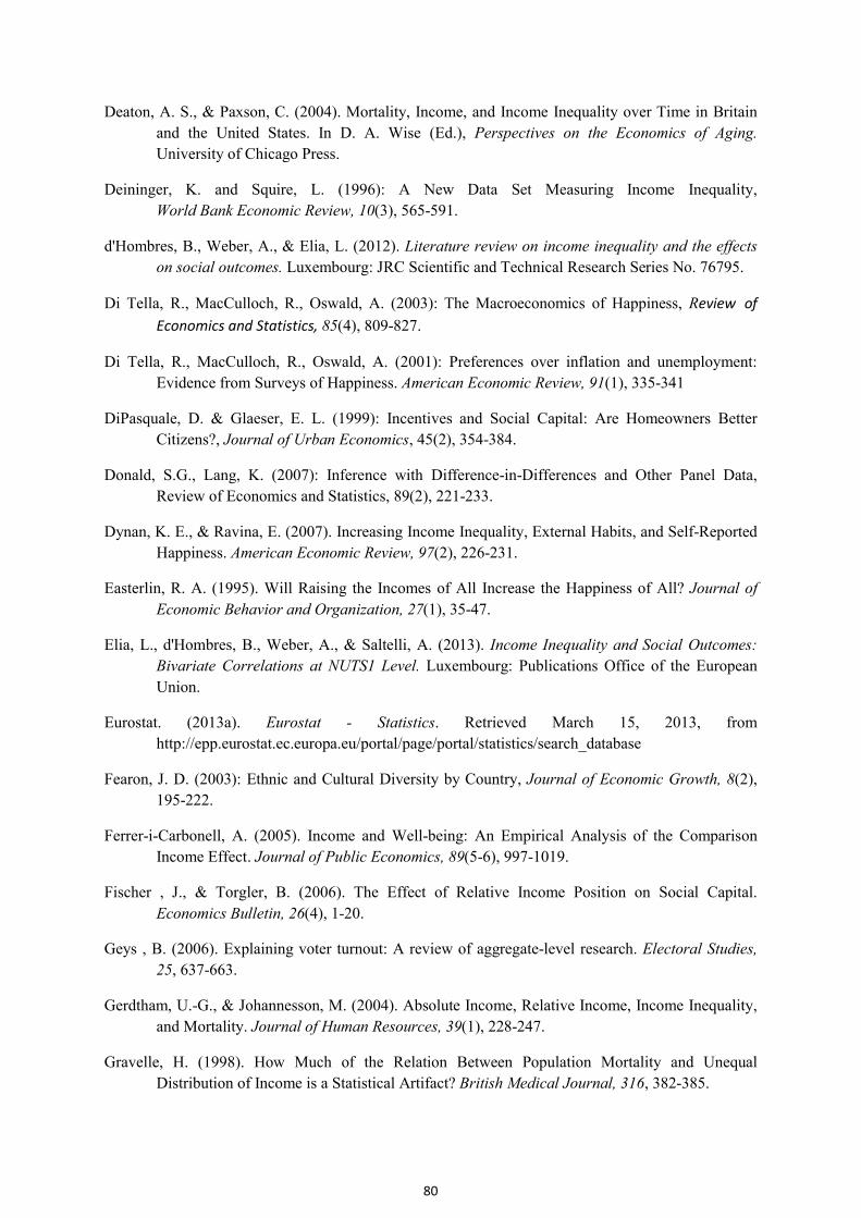
80

Deaton, A. S., & Paxson, C. (2004). Mortality, Income, and Income Inequality over Time in Britain

and the United States. In D. A. Wise (Ed.), Perspectives on the Economics of Aging.

University of Chicago Press.

Deininger, K. and Squire, L. (1996): A New Data Set Measuring Income Inequality,

World Bank Economic Review, 10(3), 565-591.

d'Hombres, B., Weber, A., & Elia, L. (2012). Literature review on income inequality and the effects

on social outcomes. Luxembourg: JRC Scientific and Technical Research Series No. 76795.

Di Tella, R., MacCulloch, R., Oswald, A. (2003): The Macroeconomics of Happiness, Review of

Economics and Statistics, 85(4), 809-827.

Di Tella, R., MacCulloch, R., Oswald, A. (2001): Preferences over inflation and unemployment:

Evidence from Surveys of Happiness. American Economic Review, 91(1), 335-341

DiPasquale, D. & Glaeser, E. L. (1999): Incentives and Social Capital: Are Homeowners Better

Citizens?, Journal of Urban Economics, 45(2), 354-384.

Donald, S.G., Lang, K. (2007): Inference with Difference-in-Differences and Other Panel Data,

Review of Economics and Statistics, 89(2), 221-233.

Dynan, K. E., & Ravina, E. (2007). Increasing Income Inequality, External Habits, and Self-Reported

Happiness. American Economic Review, 97(2), 226-231.

Easterlin, R. A. (1995). Will Raising the Incomes of All Increase the Happiness of All? Journal of

Economic Behavior and Organization, 27(1), 35-47.

Elia, L., d'Hombres, B., Weber, A., & Saltelli, A. (2013). Income Inequality and Social Outcomes:

Bivariate Correlations at NUTS1 Level. Luxembourg: Publications Office of the European

Union.

Eurostat. (2013a). Eurostat - Statistics. Retrieved March 15, 2013, from

http://epp.eurostat.ec.europa.eu/portal/page/portal/statistics/search_database

Fearon, J. D. (2003): Ethnic and Cultural Diversity by Country, Journal of Economic Growth, 8(2),

195-222.

Ferrer-i-Carbonell, A. (2005). Income and Well-being: An Empirical Analysis of the Comparison

Income Effect. Journal of Public Economics, 89(5-6), 997-1019.

Fischer , J., & Torgler, B. (2006). The Effect of Relative Income Position on Social Capital.

Economics Bulletin, 26(4), 1-20.

Geys , B. (2006). Explaining voter turnout: A review of aggregate-level research. Electoral Studies,

25, 637-663.

Gerdtham, U.-G., & Johannesson, M. (2004). Absolute Income, Relative Income, Income Inequality,

and Mortality. Journal of Human Resources, 39(1), 228-247.

Gravelle, H. (1998). How Much of the Relation Between Population Mortality and Unequal

Distribution of Income is a Statistical Artifact? British Medical Journal, 316, 382-385.

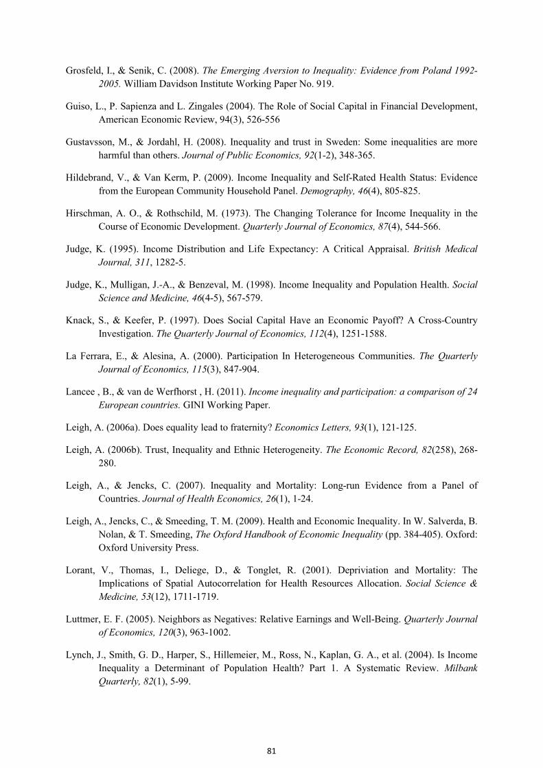
81

Grosfeld, I., & Senik, C. (2008). The Emerging Aversion to Inequality: Evidence from Poland 1992-

2005. William Davidson Institute Working Paper No. 919.

Guiso, L., P. Sapienza and L. Zingales (2004). The Role of Social Capital in Financial Development,

American Economic Review, 94(3), 526-556

Gustavsson, M., & Jordahl, H. (2008). Inequality and trust in Sweden: Some inequalities are more

harmful than others. Journal of Public Economics, 92(1-2), 348-365.

Hildebrand, V., & Van Kerm, P. (2009). Income Inequality and Self-Rated Health Status: Evidence

from the European Community Household Panel. Demography, 46(4), 805-825.

Hirschman, A. O., & Rothschild, M. (1973). The Changing Tolerance for Income Inequality in the

Course of Economic Development. Quarterly Journal of Economics, 87(4), 544-566.

Judge, K. (1995). Income Distribution and Life Expectancy: A Critical Appraisal. British Medical

Journal, 311, 1282-5.

Judge, K., Mulligan, J.-A., & Benzeval, M. (1998). Income Inequality and Population Health. Social

Science and Medicine, 46(4-5), 567-579.

Knack, S., & Keefer, P. (1997). Does Social Capital Have an Economic Payoff? A Cross-Country

Investigation. The Quarterly Journal of Economics, 112(4), 1251-1588.

La Ferrara, E., & Alesina, A. (2000). Participation In Heterogeneous Communities. The Quarterly

Journal of Economics, 115(3), 847-904.

Lancee , B., & van de Werfhorst , H. (2011). Income inequality and participation: a comparison of 24

European countries. GINI Working Paper.

Leigh, A. (2006a). Does equality lead to fraternity? Economics Letters, 93(1), 121-125.

Leigh, A. (2006b). Trust, Inequality and Ethnic Heterogeneity. The Economic Record, 82(258), 268-

280.

Leigh, A., & Jencks, C. (2007). Inequality and Mortality: Long-run Evidence from a Panel of

Countries. Journal of Health Economics, 26(1), 1-24.

Leigh, A., Jencks, C., & Smeeding, T. M. (2009). Health and Economic Inequality. In W. Salverda, B.

Nolan, & T. Smeeding, The Oxford Handbook of Economic Inequality (pp. 384-405). Oxford:

Oxford University Press.

Lorant, V., Thomas, I., Deliege, D., & Tonglet, R. (2001). Depriviation and Mortality: The

Implications of Spatial Autocorrelation for Health Resources Allocation. Social Science &

Medicine, 53(12), 1711-1719.

Luttmer, E. F. (2005). Neighbors as Negatives: Relative Earnings and Well-Being. Quarterly Journal

of Economics, 120(3), 963-1002.

Lynch, J., Smith, G. D., Harper, S., Hillemeier, M., Ross, N., Kaplan, G. A., et al. (2004). Is Income

Inequality a Determinant of Population Health? Part 1. A Systematic Review. Milbank

Quarterly, 82(1), 5-99.

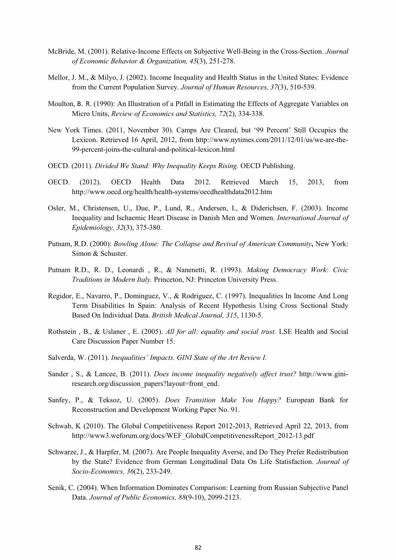
82

McBride, M. (2001). Relative-Income Effects on Subjective Well-Being in the Cross-Section. Journal

of Economic Behavior & Organization, 45(3), 251-278.

Mellor, J. M., & Milyo, J. (2002). Income Inequality and Health Status in the United States: Evidence

from the Current Population Survey. Journal of Human Resources, 37(3), 510-539.

Moulton, B. R. (1990): An Illustration of a Pitfall in Estimating the Effects of Aggregate Variables on

Micro Units, Review of Economics and Statistics, 72(2), 334-338.

New York Times. (2011, November 30). Camps Are Cleared, but ‘99 Percent’ Still Occupies the

Lexicon. Retrieved 16 April, 2012, from http://www.nytimes.com/2011/12/01/us/we-are-the-

99-percent-joins-the-cultural-and-political-lexicon.html

OECD. (2011). Divided We Stand: Why Inequality Keeps Rising. OECD Publishing.

OECD. (2012). OECD Health Data 2012. Retrieved March 15, 2013, from

http://www.oecd.org/health/health-systems/oecdhealthdata2012.htm

Osler, M., Christensen, U., Due, P., Lund, R., Andersen, I., & Diderichsen, F. (2003). Income

Inequality and Ischaemic Heart Disease in Danish Men and Women. International Journal of

Epidemiology, 32(3), 375-380.

Putnam, R.D. (2000): Bowling Alone: The Collapse and Revival of American Community, New York:

Simon & Schuster.

Putnam R.D., R. D., Leonardi , R., & Nanenetti, R. (1993). Making Democracy Work: Civic

Traditions in Modern Italy. Princeton, NJ: Princeton University Press.

Regidor, E., Navarro, P., Dominguez, V., & Rodriguez, C. (1997). Inequalities In Income And Long

Term Disabilities In Spain: Analysis of Recent Hypothesis Using Cross Sectional Study

Based On Individual Data. British Medical Journal, 315, 1130-5.

Rothstein , B., & Uslaner , E. (2005). All for all: equality and social trust. LSE Health and Social

Care Discussion Paper Number 15.

Salverda, W. (2011). Inequalities’ Impacts. GINI State of the Art Review I.

Sander , S., & Lancee, B. (2011). Does income inequality negatively affect trust? http://www.gini-

research.org/discussion_papers?layout=front_end.

Sanfey, P., & Teksoz, U. (2005). Does Transition Make You Happy? European Bank for

Reconstruction and Development Working Paper No. 91.

Schwab, K (2010). The Global Competitiveness Report 2012-2013, Retrieved April 22, 2013, from

http://www3.weforum.org/docs/WEF_GlobalCompetitivenessReport_2012-13.pdf

Schwarze, J., & Harpfer, M. (2007). Are People Inequality Averse, and Do They Prefer Redistribution

by the State? Evidence from German Longitudinal Data On Life Statisfaction. Journal of

Socio-Economics, 36(2), 233-249.

Senik, C. (2004). When Information Dominates Comparison: Learning from Russian Subjective Panel

Data. Journal of Public Economics, 88(9-10), 2099-2123.

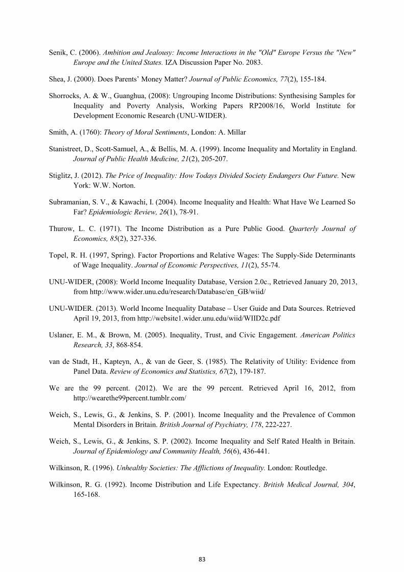
83

Senik, C. (2006). Ambition and Jealousy: Income Interactions in the "Old" Europe Versus the "New"

Europe and the United States. IZA Discussion Paper No. 2083.

Shea, J. (2000). Does Parents’ Money Matter? Journal of Public Economics, 77(2), 155-184.

Shorrocks, A. & W., Guanghua, (2008): Ungrouping Income Distributions: Synthesising Samples for

Inequality and Poverty Analysis, Working Papers RP2008/16, World Institute for

Development Economic Research (UNU-WIDER).

Smith, A. (1760): Theory of Moral Sentiments, London: A. Millar

Stanistreet, D., Scott-Samuel, A., & Bellis, M. A. (1999). Income Inequality and Mortality in England.

Journal of Public Health Medicine, 21(2), 205-207.

Stiglitz, J. (2012). The Price of Inequality: How Todays Divided Society Endangers Our Future. New

York: W.W. Norton.

Subramanian, S. V., & Kawachi, I. (2004). Income Inequality and Health: What Have We Learned So

Far? Epidemiologic Review, 26(1), 78-91.

Thurow, L. C. (1971). The Income Distribution as a Pure Public Good. Quarterly Journal of

Economics, 85(2), 327-336.

Topel, R. H. (1997, Spring). Factor Proportions and Relative Wages: The Supply-Side Determinants

of Wage Inequality. Journal of Economic Perspectives, 11(2), 55-74.

UNU-WIDER, (2008): World Income Inequality Database, Version 2.0c., Retrieved January 20, 2013,

from http://www.wider.unu.edu/research/Database/en_GB/wiid/

UNU-WIDER. (2013). World Income Inequality Database – User Guide and Data Sources. Retrieved

April 19, 2013, from http://website1.wider.unu.edu/wiid/WIID2c.pdf

Uslaner, E. M., & Brown, M. (2005). Inequality, Trust, and Civic Engagement. American Politics

Research, 33, 868-854.

van de Stadt, H., Kapteyn, A., & van de Geer, S. (1985). The Relativity of Utility: Evidence from

Panel Data. Review of Economics and Statistics, 67(2), 179-187.

We are the 99 percent. (2012). We are the 99 percent. Retrieved April 16, 2012, from

http://wearethe99percent.tumblr.com/

Weich, S., Lewis, G., & Jenkins, S. P. (2001). Income Inequality and the Prevalence of Common

Mental Disorders in Britain. British Journal of Psychiatry, 178, 222-227.

Weich, S., Lewis, G., & Jenkins, S. P. (2002). Income Inequality and Self Rated Health in Britain.

Journal of Epidemiology and Community Health, 56(6), 436-441.

Wilkinson, R. (1996). Unhealthy Societies: The Afflictions of Inequality. London: Routledge.

Wilkinson, R. G. (1992). Income Distribution and Life Expectancy. British Medical Journal, 304,

165-168.

84

Wilkinson, R. G. (1994). Health, Redistribution and Growth. In A. Glyn, & D. Miliband (Eds.),

Paying for Inequality: The Economic Cost of Social Injustice (pp. 24-43). London:

IPPE/Rivers Oram Press.

Wilkinson, R., & Pickett, K. (2009). The Spirit Level, Why More Equal Societies Almost Always Do

Better. Allen Lane.

World Bank. (2013). World Development Indicators. Retrieved March 15, 2013, from

http://data.worldbank.org/data-catalog/world-development-indicators

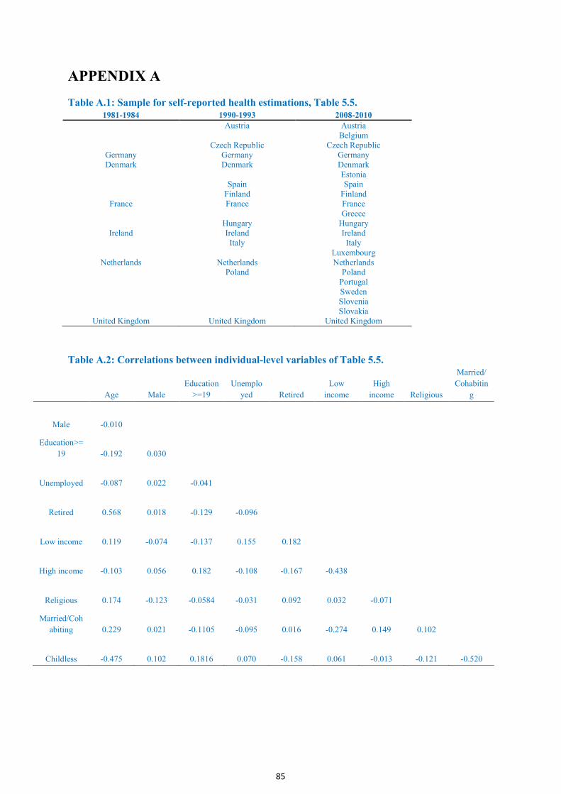
85

APPENDIX A

Table A.1: Sample for self-reported health estimations, Table 5.5. 1981-1984 1990-1993 2008-2010

Austria Austria Belgium Czech Republic Czech Republic

Germany Germany Germany Denmark Denmark Denmark

Estonia Spain Spain Finland Finland

France France France Greece Hungary Hungary

Ireland Ireland Ireland Italy Italy Luxembourg

Netherlands Netherlands Netherlands Poland Poland Portugal Sweden Slovenia Slovakia

United Kingdom United Kingdom United Kingdom

Table A.2: Correlations between individual-level variables of Table 5.5.

Age Male

Education

>=19

Unemplo

yed Retired

Low

income

High

income Religious

Married/

Cohabitin

g

Male -0.010

Education>=

19 -0.192 0.030

Unemployed -0.087 0.022 -0.041

Retired 0.568 0.018 -0.129 -0.096

Low income 0.119 -0.074 -0.137 0.155 0.182

High income -0.103 0.056 0.182 -0.108 -0.167 -0.438

Religious 0.174 -0.123 -0.0584 -0.031 0.092 0.032 -0.071

Married/Coh

abiting 0.229 0.021 -0.1105 -0.095 0.016 -0.274 0.149 0.102

Childless -0.475 0.102 0.1816 0.070 -0.158 0.061 -0.013 -0.121 -0.520

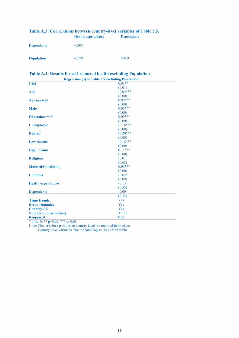
86

Table A.3: Correlations between country-level variables of Table 5.5. Health expenditure Dependents

Dependents -0.004

Population -0.206 0.109

Table A.4: Results for self-reported health excluding Population Regression (3) of Table 5.5 excluding Population

Gini 0.01** (0.01) Age -0.04*** (0.00) Age squared 0.00*** (0.00) Male 0.05*** (0.00) Education>=19 0.09*** (0.00) Unemployed -0.16*** (0.00) Retired -0.20*** (0.00) Low income -0.18*** (0.00) High income 0.11*** (0.00) Religious -0.01 (0.62) Married/Cohabiting 0.05*** (0.00) Childless -0.03* (0.09) Health expenditure -0.13 (0.55) Dependents -0.00 (0.32)

Time trends Yes

Break Dummies Yes Country-FE Yes Number of observations 37188 R-squared 0.22 * p<0.10, ** p<0.05, *** p<0.01 Note: Cluster robust p-values at country level are reported in brackets Country level variables take the same lag as the Gini variable.

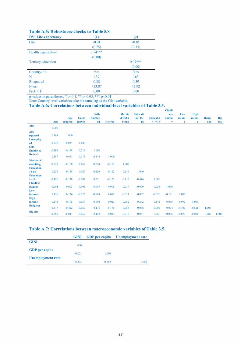
87

Table A.5: Robustness-checks to Table 5.8 DV: Life-expectancy (1) (2)

Gini -0.01 -0.05

(0.75) (0.15)

Health expenditure 3.74***

(0.00)

Tertiary education 0.07***

(0.00)

Country-FE Yes Yes

N 139 163

R-squared 0.88 0.39

F-test 413.87 42.92

Prob > F 0.00 0.00

p-values in parentheses, * p<0.1, ** p<0.05, *** p<0.01 Note: Country level variables take the same lag as the Gini variable.

Table A.6: Correlations between individual-level variables of Table 3.5.

Age

Age

squared

Unem

ployed

Self-

Employ

ed Retired

Marrie

d/Coha

biting

Educati

on 15-

18

Educatio

n >=19

Childl

ess

dumm

y

Low

incom

e

High

incom

e

Religi

ous

Big

city

Age 1.000

Age

squared 0.988 1.000

Unemploy

ed -0.028 -0.037 1.000

Self-

Employed -0.199 -0.198 -0.719 1.000

Retired 0.587 0.641 -0.015 -0.144 1.000

Married/C

ohabiting -0.098 -0.100 0.062 -0.054 -0.113 1.000

Education

15-18 0.136 0.158 0.037 -0.159 0.192 0.146 1.000

Education

>=19 -0.121 -0.138 -0.084 0.211 -0.173 -0.110 -0.446 1.000

Childless

dummy -0.004 -0.003 0.005 0.019 0.008 0.017 -0.070 0.056 1.000

Low

income 0.136 0.136 -0.022 -0.063 0.092 -0.031 0.032 -0.056 -0.131 1.000

High

income 0.243 0.195 0.030 -0.096 0.023 -0.082 -0.242 0.142 0.035 0.092 1.000

Religious -0.477 -0.422 -0.067 0.176 -0.170 0.058 0.038 -0.001 0.094 -0.100 -0.521 1.000

Big city -0.050 -0.047 -0.062 0.118 -0.039 -0.016 -0.031 0.066 -0.006 -0.070 -0.081 0.089 1.000

Table A.7: Correlations between macroeconomic variables of Table 3.5.

GINI GDP per capita Unemployment rate

GINI 1.000

GDP per capita -0.201 1.000

Unemployment rate 0.292 -0.152 1.000

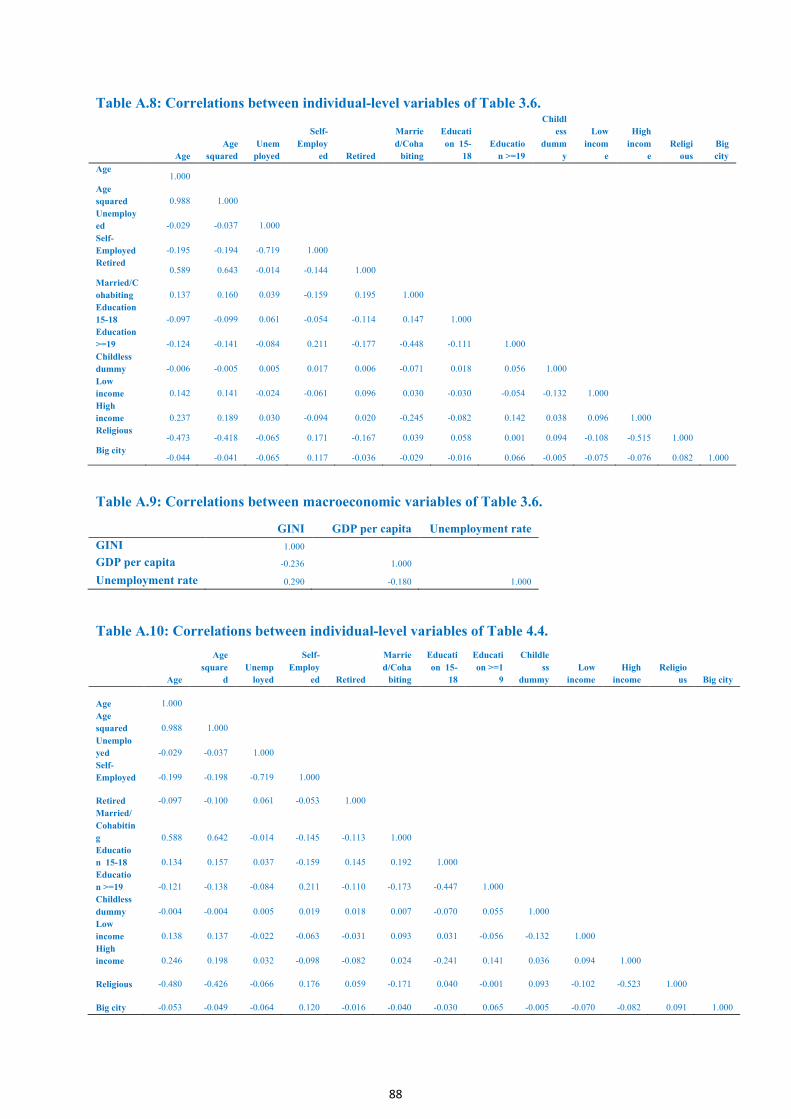
88

Table A.8: Correlations between individual-level variables of Table 3.6.

Age

Age

squared

Unem

ployed

Self-

Employ

ed Retired

Marrie

d/Coha

biting

Educati

on 15-

18

Educatio

n >=19

Childl

ess

dumm

y

Low

incom

e

High

incom

e

Religi

ous

Big

city

Age 1.000

Age

squared 0.988 1.000

Unemploy

ed -0.029 -0.037 1.000

Self-

Employed -0.195 -0.194 -0.719 1.000

Retired 0.589 0.643 -0.014 -0.144 1.000

Married/C

ohabiting 0.137 0.160 0.039 -0.159 0.195 1.000

Education

15-18 -0.097 -0.099 0.061 -0.054 -0.114 0.147 1.000

Education

>=19 -0.124 -0.141 -0.084 0.211 -0.177 -0.448 -0.111 1.000

Childless

dummy -0.006 -0.005 0.005 0.017 0.006 -0.071 0.018 0.056 1.000

Low

income 0.142 0.141 -0.024 -0.061 0.096 0.030 -0.030 -0.054 -0.132 1.000

High

income 0.237 0.189 0.030 -0.094 0.020 -0.245 -0.082 0.142 0.038 0.096 1.000

Religious -0.473 -0.418 -0.065 0.171 -0.167 0.039 0.058 0.001 0.094 -0.108 -0.515 1.000

Big city -0.044 -0.041 -0.065 0.117 -0.036 -0.029 -0.016 0.066 -0.005 -0.075 -0.076 0.082 1.000

Table A.9: Correlations between macroeconomic variables of Table 3.6.

GINI GDP per capita Unemployment rate

GINI 1.000

GDP per capita -0.236 1.000

Unemployment rate 0.290 -0.180 1.000

Table A.10: Correlations between individual-level variables of Table 4.4.

Age

Age

square

d Unemp

loyed

Self-

Employ

ed Retired

Marrie

d/Coha

biting

Educati

on 15-

18

Educati

on >=1

9

Childle

ss

dummy Low

income High

income Religio

us Big city

Age 1.000

Age

squared 0.988 1.000

Unemplo

yed -0.029 -0.037 1.000

Self-

Employed -0.199 -0.198 -0.719 1.000

Retired -0.097 -0.100 0.061 -0.053 1.000

Married/

Cohabitin

g 0.588 0.642 -0.014 -0.145 -0.113 1.000

Educatio

n 15-18 0.134 0.157 0.037 -0.159 0.145 0.192 1.000

Educatio

n >=19 -0.121 -0.138 -0.084 0.211 -0.110 -0.173 -0.447 1.000

Childless

dummy -0.004 -0.004 0.005 0.019 0.018 0.007 -0.070 0.055 1.000

Low

income 0.138 0.137 -0.022 -0.063 -0.031 0.093 0.031 -0.056 -0.132 1.000

High

income 0.246 0.198 0.032 -0.098 -0.082 0.024 -0.241 0.141 0.036 0.094 1.000

Religious -0.480 -0.426 -0.066 0.176 0.059 -0.171 0.040 -0.001 0.093 -0.102 -0.523 1.000

Big city -0.053 -0.049 -0.064 0.120 -0.016 -0.040 -0.030 0.065 -0.005 -0.070 -0.082 0.091 1.000

89

90

European Commission

EUR 26488 – Joint Research Centre – Institute for the Protection and Security of the Citizen

Title: Multivariate analysis of the effect of income inequality on health, social capital, and happiness

Author(s): Beatrice d’Hombres, Leandro Elia, Anke Weber

Luxembourg: Publications Office of the European Union

2013 –90pp. – 21.0 x 29.7 cm

EUR – Scientific and Technical Research series – ISSN 1831-9424 (online)

ISBN 978-92-79-35414-4

doi: 10.2788/68427

Abstract

The last two decades have seen a growing concern about rising inequality. In a recent book (2012), Economics

Nobel laureate Joseph Stiglitz argues that rising income inequality is one of the main factors underlying the

economic and financial crisis in the United States. Wilkinson and Pickett (2009) similarly assert that higher

inequality has harmful social consequences. This trend of growing inequality has furthermore been condemned in

public arenas, where protests in the United States (the “Occupy Wall Street” movement) and in Spain (the

“indignados”) show the extent of widespread public dissatisfaction with the present system which is denounced as

being fundamentally flawed and unfair. The “We are the 99%” slogan and the associated web blog “We are the 99

percent” are direct references to this growing unequal distribution of wealth. A common rallying point of these

movements is the argument that bankers who have benefited from large bonuses have been protected by bailout

measures, while the victims of the crisis brought on by these very same bankers are faced with the reality of rising

unemployment. This has also recently led the EU to agree on capping bonuses to bankers.

Within this context, the European Commission decided last year to undertake a comprehensive study on the social

and economic challenges associated with rising income inequality in Europe. This report constitutes the third

deliverable of this global study. The first report includes a literature review on the relationship between income

inequality and social outcome variables in the areas of happiness, criminality, health, social capital, education,

voting behavior and female labor participation (d'Hombres, Weber, & Elia, 2012). The second report complements

the literature review by examining the bivariate correlations on NUTS1 level between income inequality and the

social outcomes mentioned above (Elia, d'Hombres, Weber, & Saltelli, 2013). In this third report, we carry out a

multivariate analysis on a selected number of social outcomes while controlling for a multitude of individual and

country level specificities. The social outcomes are social capital, i.e. trust and participation in organizations,

happiness and health.

This study suggests that the adverse effect of income inequality on a plurality of societal development challenges

as proposed by Wilkinson and Pickett (2009) cannot be confirmed by the data, except for the case of trust. In

particular, our analysis cannot confirm the hypothesis of a strong and significant effect of income inequality on

health, happiness and participation in associational activities.

However, we show that income inequality has a potential damaging effect on trust in Europe. A negative

association between income disparities and generalized trust is reported in all estimations presented in this report.

Though these findings need to be considered with care given that they might be specific to the countries sampled

or the time period covered, the implication of a significant effect of inequality on trust should not be discounted.

According to a variety of scholars, trust is critical for the functioning of societies (Putnam, 2000). Social capital and

trust are factors which are linked to cooperative behaviors and investment decisions as well as to the quality of

institutions, which in turn are all key factors of economic performance (Knack and Keefer, 1996, and Guiso et al

2004).

z

As the Commission’s in-house science service, the Joint Research Centre’s mission is to provide EU policies with independent, evidence-based scientific and technical support throughout the whole policy cycle. Working in close cooperation with policy Directorates-General, the JRC addresses key societal challenges while stimulating innovation through developing new standards, methods and tools, and sharing and transferring its know-how to the Member States and international community. Key policy areas include: environment and climate change; energy and transport; agriculture and food security; health and consumer protection; information society and digital agenda; safety and security including nuclear; all supported through a cross-cutting and multi-disciplinary approach.

LBN

A26488EN

N