Embed Size (px)
Citation preview
LARS Contract Report 112678 NASA CRshy160113
Final Report Vol 11Multispectral Scanner System
Parameter Study and Analysis Software System Description by B G Mobasseri Made available under NASA sponsorufR$-D J Wiersma inthe interest of early and wide disshy
somrnition of Earth Resources SurveyE R Wiswell Ptogram information and without liability
D A Landgrebe -any use made thereof
C D McGillem PE Anuta
Principal Investigator D A Landgrebe
November 1978(E79-10162) MULTISPECTRAVSCARNER SYSTEM N1721517 PARABETER STUDY AND ANALYSIS-SOF-TWARE SYSTEM DESCRIPTION-VOLUME 2 Finai Rleport-1 Dec 1977 - 30 NOV 1978 JPurdue Uni-v ) 133 p HC Unclds A07MT A01 - -CSCI-09B G343 00162
Prepared for National Aeronautics and Space Administration Johnson Space Center Earth Observation Division Houston Texas 77058 Contract No NAS9-15466 Technical Monitor J D EricksonSF3
Submitted byLaboratory for Applications of Remote SensingPurdue University West Lafayette Indiana 47907
TAP TJ0FOnMATTOrr FOPji
1 Report No 2 Government Accession No 3 Recipienrs Catalog No
112678 4 Title and Subtitle 5- Report Date
Multispectral Scanner System Parameter Study and Analysis November 1978 Software System Description 6 Performing Organization Code
7 Author(s) 8 Performing Organization Report No
B G Mobasseri D J Wiersma E R Wiswell D A 112678 Landgrebe C D McGillem-p E Anuta 10 Work Unit No
9 Performing Organization Name and Address
Laboratory for Applications of Remote Sensing 11 Contract or Grant No Purdue University West Lafayette Indiana 47906 NAS9-15466
13 Type of Report and Period Coveed 12 Sponsoring Agency Name and Address
Final Report 12l77-l13078 J D EricksonSF3 14 Sponsoring Agency Code NASAJohnson Space Center Houston Texas 77058
15 Supplementary Notes
D A Landgrebe was LARS principal investigator
16 Abstract
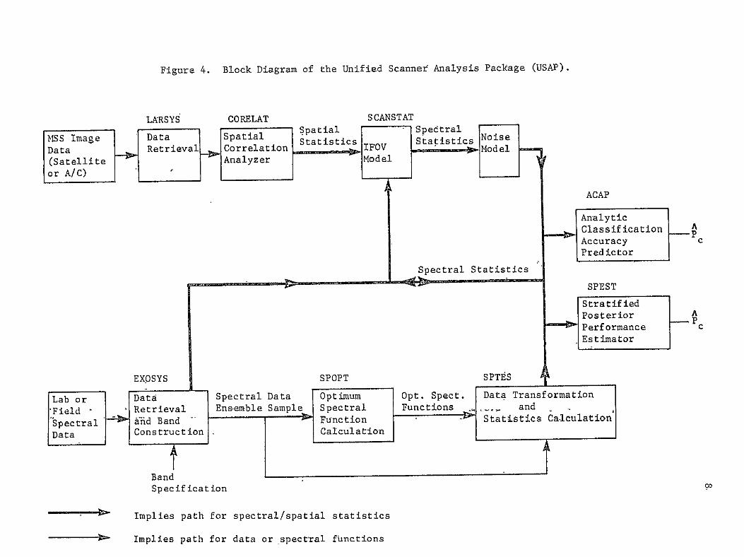
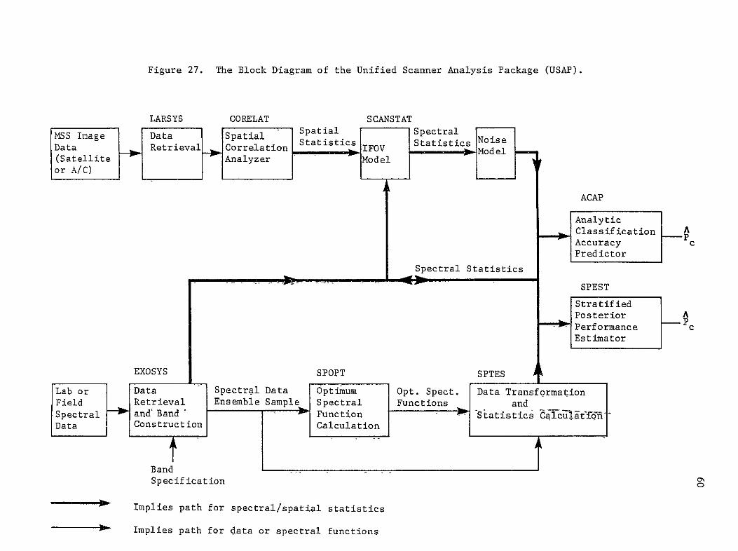
This report represents the culmination of three major pieces of research effort in defining and evaluating the performance of the next generation of multispectral scanners within the framework of a set of analytic analysis packages The integration of the available methods provides the analyst with the Unified Scanner Analysis Package (USAP) the flexibility and versatility of which is superior to many previous integrated techniques USAP consists of three main subsystems (a) a spatial path (b) a spectral path and (c) a set of analytic classification accuracy estimators which evaluate the system performance The spatial path consists of satellite andor aircraft data data spatial correlation analyzer scanner IFOV and random noise model The output of the spatial path is fed into the Analytic Classificati Accuracy Predictor (ACAP) The spectral path consists of laboratory andor field spectral data EXOSYS data retrieval optimum spectral function calculation data transformation and statistics calculation The output of the spectral path is fed into the Stratified Posterior Performance Estimator (SPEST) A brief theoretical exposition of the USAP individual buildin blocks are presented and example outputs produced References are provided for a more complete coverage of the algorithms- Each building block carries with it at least one softshyware unit The programming provides a complete input-output compatibility among these units One test case starting from the raw data base is carried through the system and the pershyformance figures in terms of a set of classification accuracies are produced A listing of the underlying software is provided in Appendix I
17 Key Words (Suggested by Author(s)) 18 Distribution Statement
Multispectral scanner USAP spatial path spectral path classification accuracy estimators IFOV model optimum spectral function calculation optimum band selection
19 Security Classif (of this report) 20UScu a ssif (of this page) - 21 No of Pages 22 Prce
Unclassified
Io0 ale by
-
nclssIfied tv
Me Nti onaN~ 0 I 1 nh ical1i110111idt011
fll~Il~tNASA
glVr2
SCrvice Spi Ingfaidd Virginia 221I6 1
TABLE OF CONTENTS
Page
List of Figures ii
List of Tables iv
1 Introduction 1
2 Scanner Parameters Analysis techniques 7
3 The Unified Scanner Analysis Package Block Diagram 59
4 Users Guide to USAP 70
5 Summary 93
6 References 98
Appendix I i 100
LIST OF FIGURES
Page
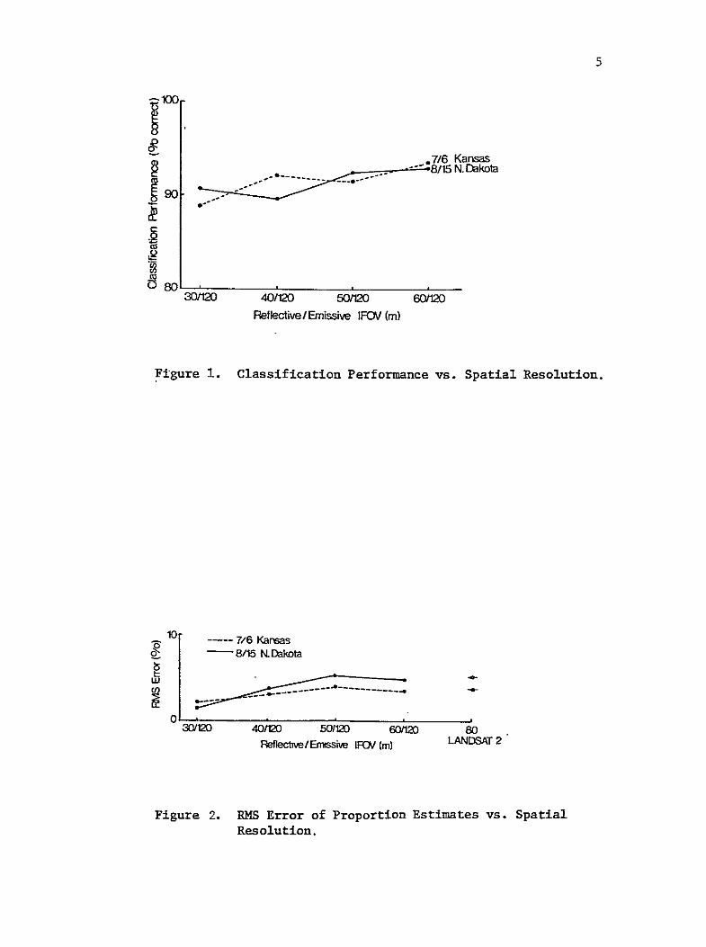
Figure 1 Classification Performance vs Spatial Resolution 5
Figure 2 RMS Error of Proportion Estimates vs Spatial Resolution 5
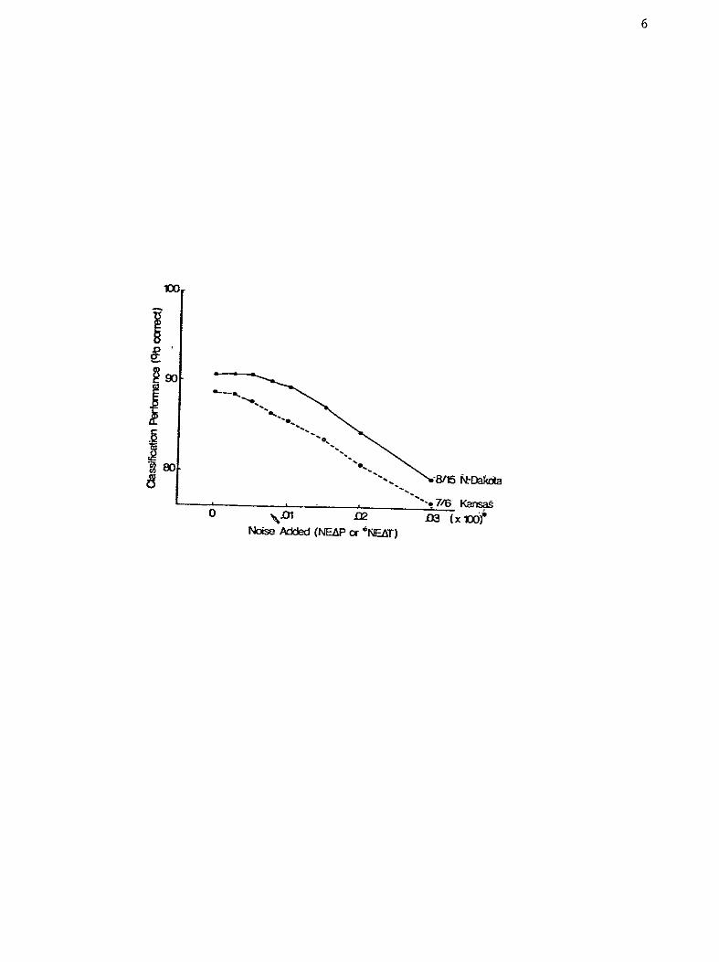
Figure 3 Classification Performance vs Noise Added for 30120 Meter Resolution 6
Figure 4 Block Diagram of the Unified Scanner Analysis Package
Figure 5 Allocation of a Measurement Vector X to an Appropriate
Figure 6 A Conceptual Illustration of the ACAP Error Estimation
Figure 7 ACAP Classification Accuracy Estimate vs Grid Size for
(USAP) S8
Partition of the FeatureSpace 10
Technique Using Two Features 15
the Test Population Data 16
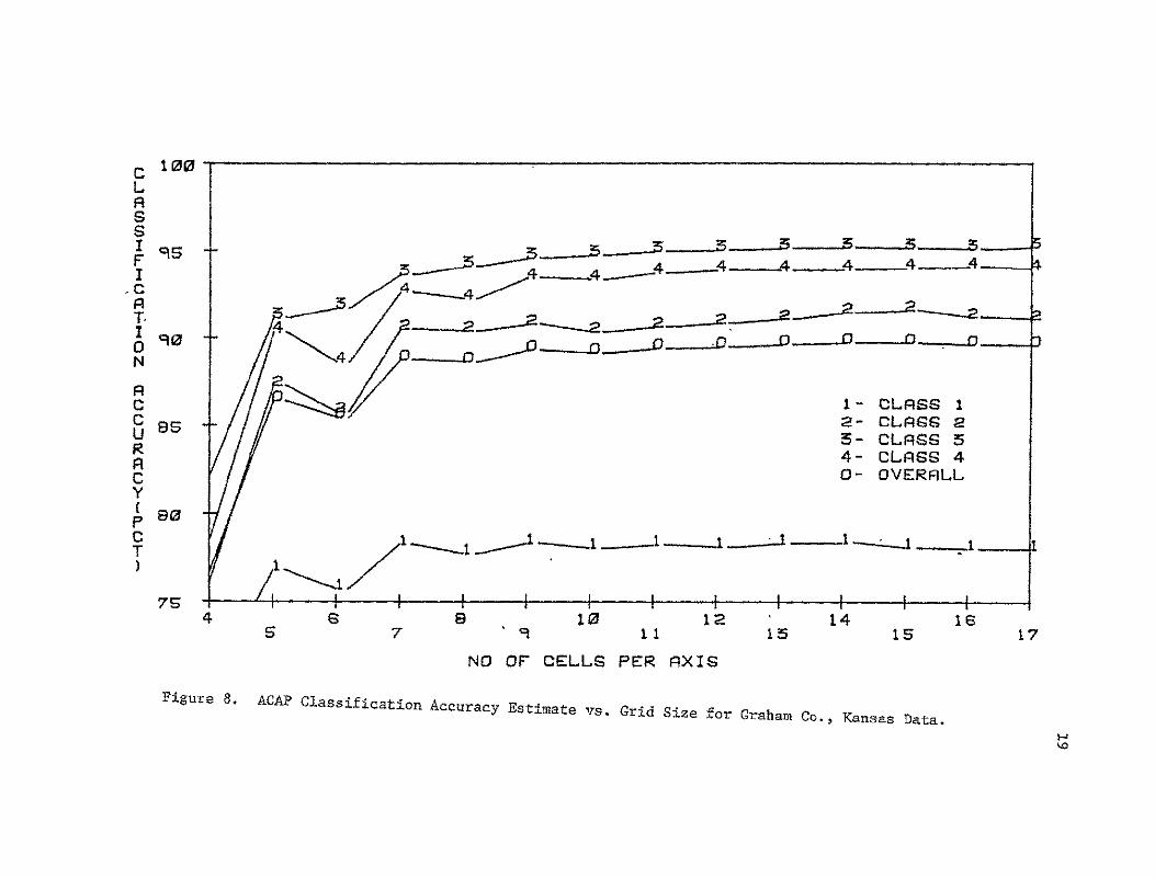
Figure 8 ACAP Classification Accuracy Estimate vs Grid Size for Graham Co Kansas Data 19
Figure 9 Scanner Spatial Model as a Linear System 27
Figure 10 Scanner Characteristic Function vs Scene Correlation
Adjacent Line Correlation = 65 31
Figure 11 Scanner Characteristic Function vs Scene Correlation Adjacent Line Correlation = 8 32
Figure 12 Scanner Characteristic Function vs Scene Correlation
Figure 13 Scanner Characteristic Function vs Scene Correlation
Figure 14 Scanner Output Classification Accuracy vs IFOV
Figure 15 Scanner Output Classification Accuracy vs IFOV
Figure 16 Scanner Output Classification Accuracy vs IFOV
Adjacent Line Correlation = 1 33
Adjacent Line Correlation = 8 34
Adjacent Sample Correlation = 55 36
Adjacent Sample Correlation = 8 37
Adjacent Sample Correlation = 95 38
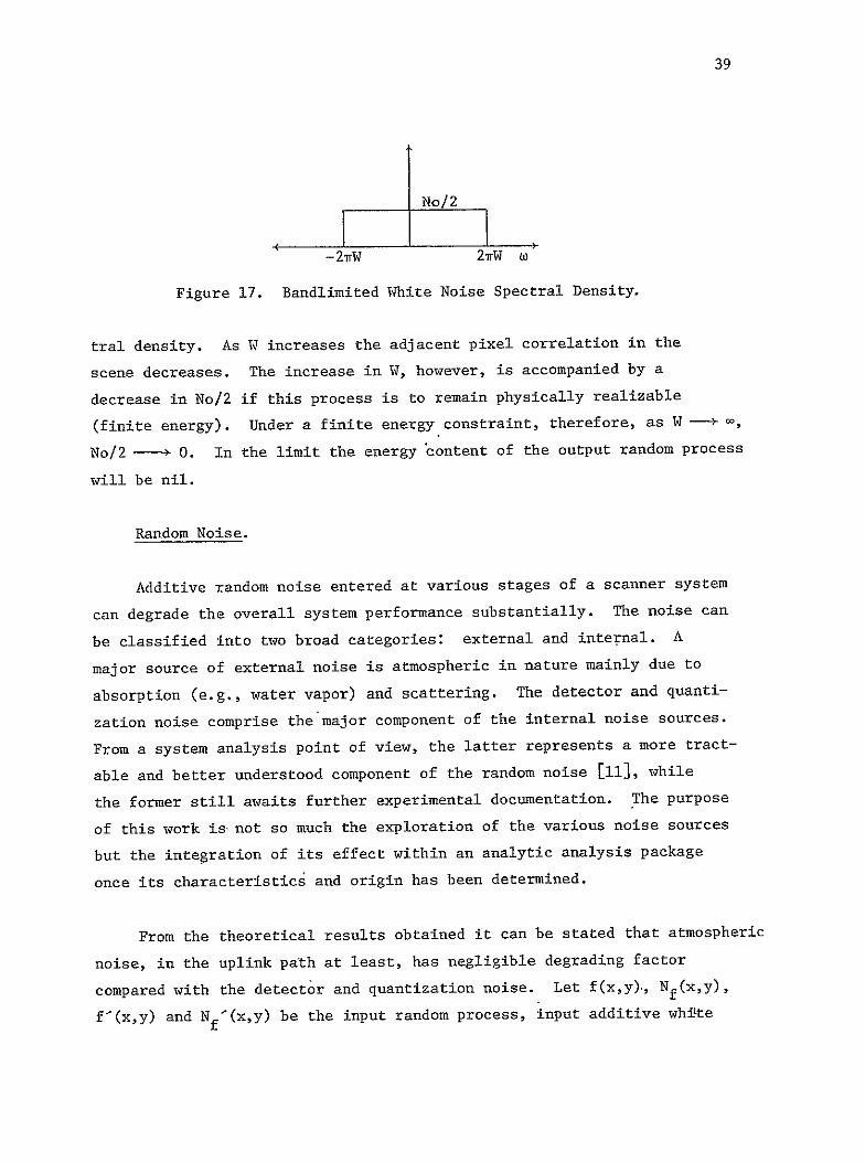
Figure 17 Bandlimited White Noise Spectral Density 39
Figure 18 Overall Output Classification Accuracy Variation with Noise and IFOV 42
Figure 19 Realization of a Stratum as the Ensemble of Spectral Samplamp Functions 45
Figure 20 Basis Function Expansion of a Random Process 46
Figure 21 Average Spectral Response -- Wheat Scene 53
Figure 22 Average Spectral Response -- Combined Scene 53
iii
Figure 23 Average nrru4tfon Bnd 1 Wheat Scene 56 Figure 24 Average Infornation Bqnd -Combned Ste 56
Figure 25 Average Informatiq Bande7 Wheat Scee 57
Figure 26 Average Infonatiopn 1i4d 7 iombnSsc e 57 Figure 27 The Block Diagvam of the Unified Scanqxxr Anaiysis
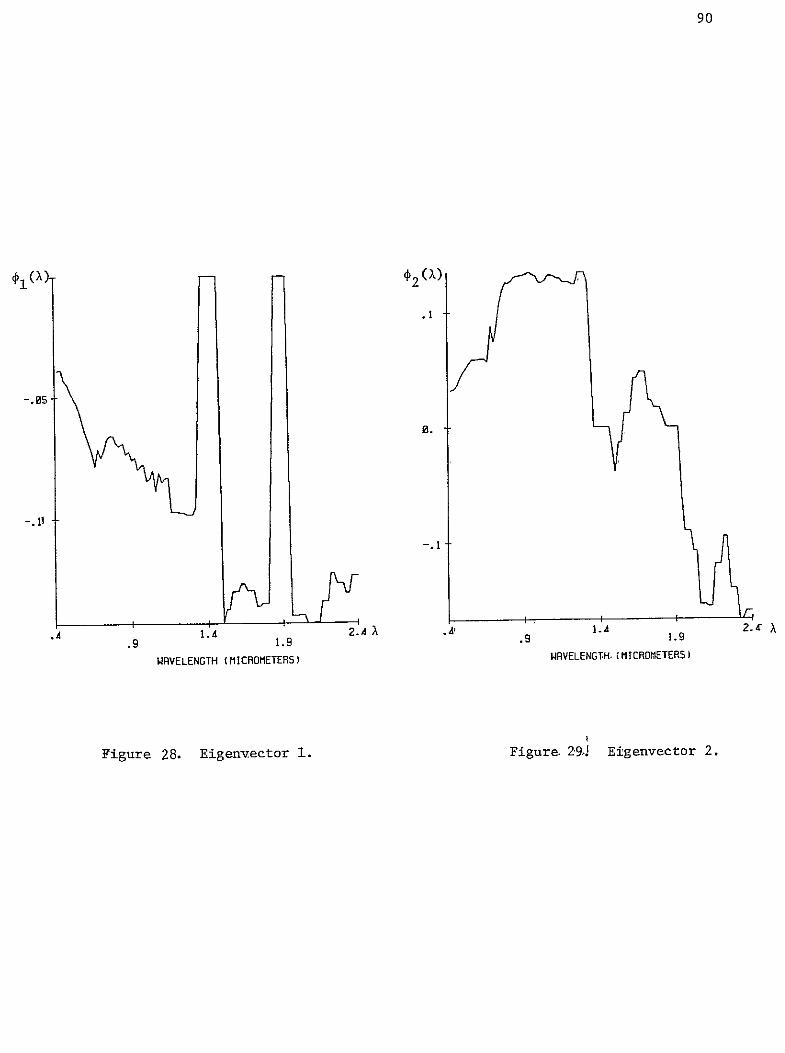
Figure 28 Eigevector 1
Package 4USAP) 60 90
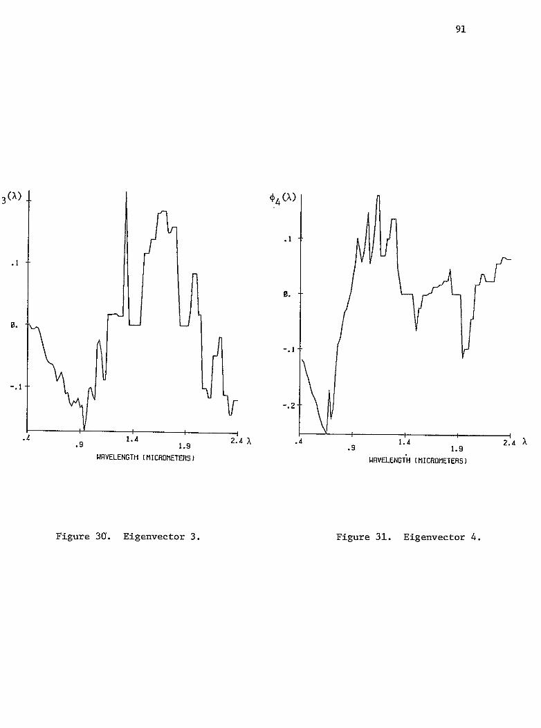
Figure 29 Eigenvector 2 0-
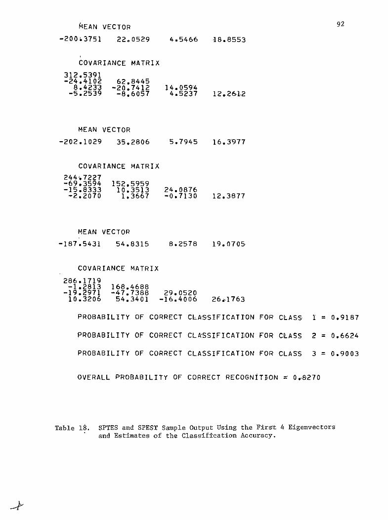
Figure 3a Eigenvector 3 91
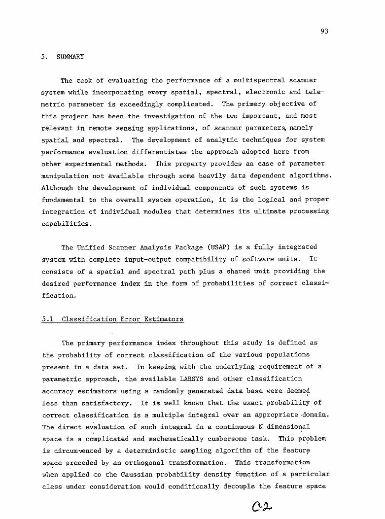
Figure 31 Eigenvector 4 9i
iv
LIST OF TABLES
Page
Table 1 ACAP and LARSYS Performance Comparison 17
Eigenvectors and Estimates of the Classification
Table 2 ACAP and LARSYS Performance Comparison Simulated Data 17
Table 3 Test of the SPEST Error Estimate 24
Table 4 Variation of Estimates 25
Table 5 Spectral Bands for Wheat Scene 52
Table 6 Spectral Bands for Combined Scene 52
Table 7 Modeling of the Wheat Scene 54
Table 8 Modeling of the Combined Scene 54
Table 9 Average Information for Wheat Scene Bands 55
Table 10 Average Information for Combined Scene Band 58
Table 11 Order of Preference of Spectral Bands for the Wheat and Combined Scenes 58
Table 12 Error Matrix for Cross Correlation Function Approximashytion Between Channels 2 and 8 64
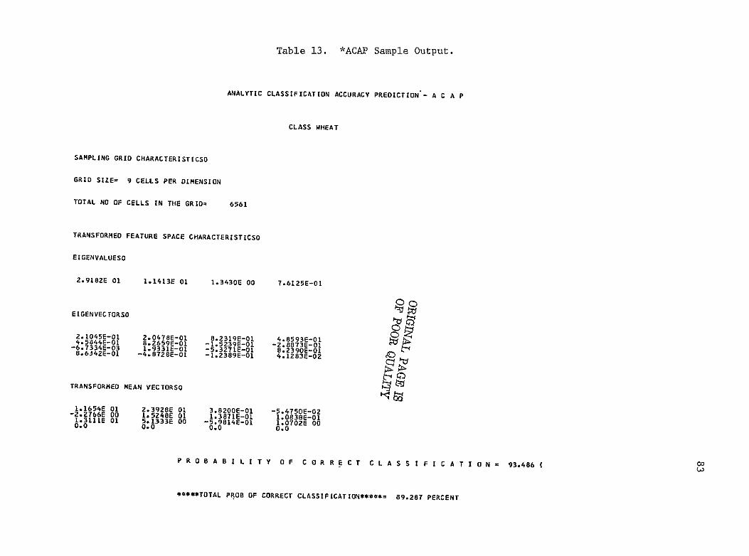
Table 13 ACAP Sample Output 83
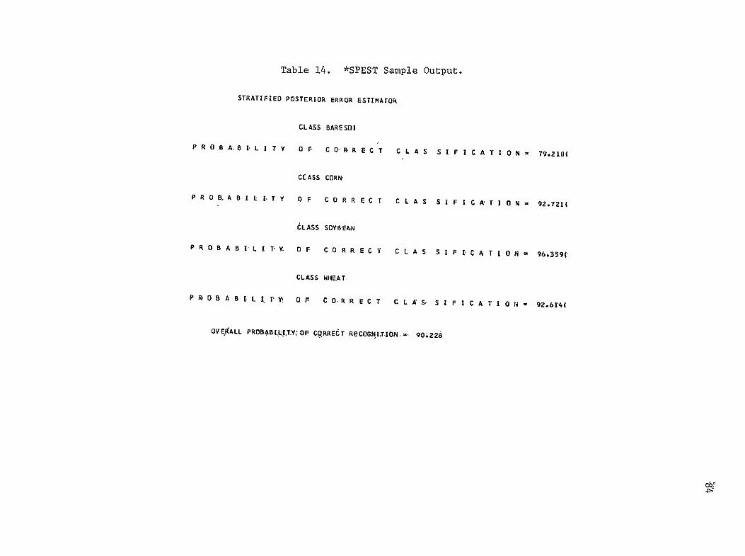
Table 14 SPEST Sample Output 84
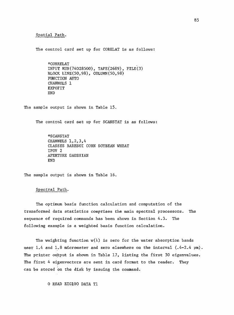
Table 15 CORRELAT Sample Output 86
Table 16 SCANSTAT Sample Output 87
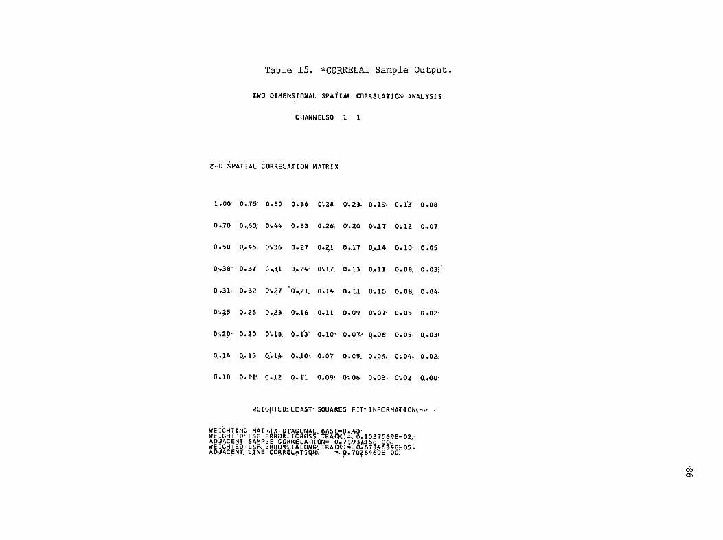
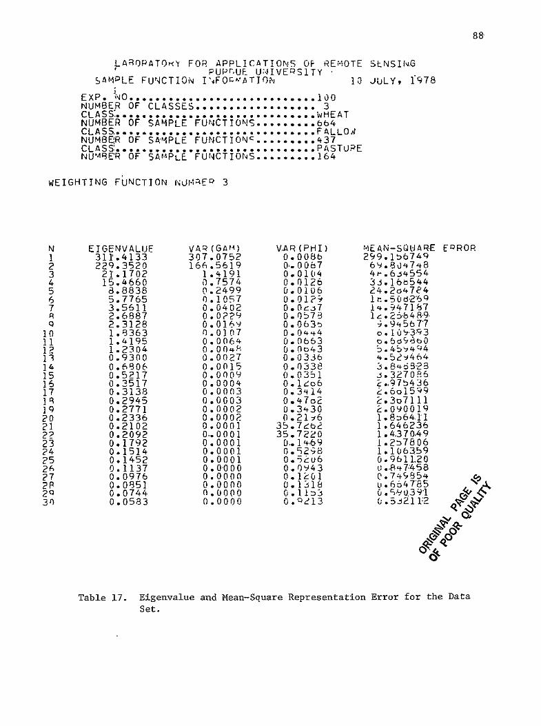
Table 17 Eigenvalue and Mean-Square Representation Error for the Data Set 88
Table 18 SPTES and SPEST Sample Output Using the First 4
Accuracy 92
Cl- Multispectral Scanner System Parameter Study and
Analysis Software System Description
1 INTRODUCTION
The utilization of sensors on earth orbiting platforms as the main
element of an Earth Observational System has undergone substantial
growth in recent years ERTS-l (Landsat-l) followed by Landsat-2 and
-3 have proven exceptionally successful in collecting data to help
monitor the Earths resources
The principal data collection unit aboard the first three Landsats
is the multispectral scanner known as MSS Although this scanner has
been providing data with a quality which exceeded most prelaunch
expectations it has been clear from the beginning that MSS does not
represent the ultimate in multispectral instruments more advanced
instruments providing greater detail would be needed as the user community
begins to become familiar with the use of such space data
The design of a multispectral scanner is a very complex matter
many different interacting factors must be properly taken into account
Currently operational systems such as MSS have been designed primarily
using subjective judgements based upon experience with experimental
data In designing a scanner the use of empirical methods at least in
part is essential Each of the large collections of scenes which a
given scanner will be used upon is a very complex information source not
enough is known to make a simple (or even a complex) model of it by
which to make the design of a scanner a simple straightforward exercise
of a mathematical procedure
And yet more is known than when MSS was designed and it is imporshy
tant to be able to carry out future designs on a more objective basis
than in the past Thus the purpose of the present work is the developshy
ment of appropriate mathematical design machinery within a theoretical
framework to allow (a) formulation of an optimum multispectral scanner
The work in this report was done under Task 22C1 Multisensor Parametric
Evaluation and Radiometric Correction Model
2
system according to defined conditions of optimality and (b) an ability
for convenient manipulation of candidate system parameters so as to
Permit comparison of the theoretically optimum designs with that of
practical approximations to it
In order to deal with the complexity of the design situation the
first step is to determine a suitable set of parameters which adequately
characterize it but is not so large as to be unmanageable It has been
observed [i] that there are five major categories of parameters which
are significant to the representation of information in remotely sensed
data They are
1 The spatial sampling scheme
2 The spectral sampling scheme
3 The signal-to-noise ratio
4 The ancillary data type and amount
5 The informational classes desired
Thus it is necessary to have present in the design machinery some means
for evaluating the impact of change in parameter values in each of these
five categories
Such a scanner design tool has been assembled in the form of a
software package for a general purpose computer Each of the parts of
this package called Unified Scanner Analysis Package (USAP) has been
carefully devised and the theory related to it fully documented [2 3 4 51
The goal of this report is to provide a documentation and description of
the software In constructing this documentation it was a~sumed that this
package will be useful for sometime into the future however it was also
assumed that it will only be used by a small number of highly knowledgeshy
able scientists
Section 2 recaps the theoretical concepts behind some of the primary
These are divi7ded into (a) scanner spatial charactershycomponents of USAP
istics modeling and noise effects (b) optimum spectral basis function
calculations (c) analytical classification accuracy predictions
3
(d) stratified posterior classification estimation and (e) an information
theory approach to band selection Although (e) is not a part of the
USAP system the results from this approach are helpful in understanding
the scanner design problem
Section 3 shows the integration of the above modules into the
software system Section 4 is the users guide to USAP describing the
required inputs and the available output products A listing of all
programs is provided in the appendix
The work which led to USAP was immediately preceded by a simulation
study of possible parametric values for the Thematic Mapper a new
scanner now being constructed for launch on Landsat-D in 1981 The
purpose of this simulation was to compare the performance for several
proposed sets of parameters We will conclude this introductory section
by briefly describing this work because it provides useful background
and serves well to illustrate the problem A more complete description
of this simulation study is contained in [l 6]
The general scheme used was to simulate the desired spaceborne
scanner parameter sets by linearly combining pixels and bands from (higher
resolution) airborne scanner data to form simulated pixels adding
noise as needed to simulate the desired SIN the data so constructed
was then classified using a Gaussian maximum likelihood classifier and
the performance measured The problem was viewed as a search of the
five dimensional parameter space defined above with the study localized
around the proposed Thematic Mapper parameters The scope of the
investigation was primarily limited to three parameters (a) spatial
resolution (b) noise level and (c) spectral bands Probability of
correct classification and per cent correct area proportion estimation
for each class were the performance criteria used The major conclusions
from the study are as follows
4
1 There was a very small but consistent increase in identification
accuracy as the IFOV was enlarged This is presumed to stem
primarily from the small increase in signal-to-noise ratio with
increasing IFOV Figure 1
2 There was a more significant decrease in the mensuration accuracy
as the IFOV was enlarged Figure 2
The noise parameter study proved somewhat inconclusive due to3
the greater amount of noise present in the original data than
desired For example viewing Figure 3 moving frolm right to
left it is seen that the classification performance continues
the amount of noise added is decreased until theto improve as
point is reached where the noise added approximately equals that
already initially present Thus it is difficult to say for
what signal-to-noise ratio a point of diminishing return would
have been reached had the initial noise not been present
4 The result of the spectral band classification studies may also
be clouded by the noise originally present in the data The
relative amount of that change in performance due to using
80-91 jimdifferent combinations of the 45-52 Jm 74-80 vtm
and 74-91 Pm bands is slight but there appears to be a slight
preference for the 45-52 jim band The performance improvement
of the Thematic Mapper channels over those approximating Landsat-l
and -2 is clear however
5 Using spectrometer data it was verified that the 74-80 vm and
80-91 Pm bands are highly correlated
6 Correlation studies also showed that the range from 10-13 Pm
is likely to be an important area in discriminating between earth
surface features Further it is noted that the absolute
calibration procedure described above results in a global
atmosphere correction of a linear type in that assuming a
uniform atmosphere over the test site the calibration
procedure permits a digital count number at the airborne
scanner output to be related directly to the present reflectance
of a scene element
The noise level in the original AC data was equivalent to about 005 NEAp
on the abscissa See Reference [ll
-----------------
5
10shy
-815 NDakota
Reflective Emissive IFOV Wm
Figure 1 Classification Performance vs Spatial Resolution
10 ---- 76 Kansas 0 815 U Dakota
0 30tO 40120 5012D 6012 80
ReflectiveEmrssive IFO( m) LANDSAT 2
Figure 2 RMS Error of Proportion Estimates vs Spatial Resolution
Nois Aded (EAPor4~c610c
geo
DL -Mshy7 0 or D2 D3 (x -0o6f
7
2 SCANNER PAPAMETERS ANALYSIS TECHNIQUES
Based upon the parametric approach introduced above the development
of a parametric scanner model must give explicit concern for the spatial
spectral and noise characteristics of the systems This is what has been
done in the Unified Scanner Analysis Package (USAP) shown in Figure 4
USA is composed of two distinct subsystems The spatial aspect of it
contains (a) a data spatial correlation analyzer (b) a scanner IFOV
model and (c) a random noise model The spectral techniques are capable
of producing an optimum spectral representation by modeling the scene as
a random process as a function of wavelengthfollowed by the determination
of optimum generalized spectral basis functions Conventional spectral
bands can also be generated Also studied was an information theory
approach using maximization of the mutual information between the reflected
and received (noisy) energy The effect of noise in the data can be
simulated in the spectral and spatial characteristics Two different data
bases are used in the system The spectral techniques require field
spectral data while the spatial techniques require MSS generated data
aircraft andor satellite The system performance defined in terms of
the classification accuracy is evaluated by two parametric algorithms
A detailed system description and users guide is presented in Sections 3
and 4 In the following the theoretical ideas behind the five major
elements of USAP are discussed
21 Analytical Classification Accuracy Prediction
Throughout the analysis of remotely sensed data the probability of
correct classification has ranked high among the set of performance indices
available to the analyst This is particularly true in a scanner system
modeling where generally the optimization of various system parameters
has as its prime objective the maximization of the classification accuracy
of various classes present in the data set
The estimation of the classification accuracy is fairly straightforshy
ward if Monte-Carlo type methods are employed In system simulation and
modeling however such approaches are generally a handicap due to their
Figure 4 Block Diagram of the Unified Scanner Analysis Package (USAP)
LARSYS CORELAT SCANSTAT
MSS Image Data Spatial Statistics statistics Noise Data Retrieval Correlation IFOlV Model
M(Satelliteod [or AC) In l zeA
A P~
SAnalytic
AClassification - Accuracy -Pc Predictor
Spectral Statistics
SPEST
Stratified Posterior A
Performance
Estimator
EXPSYS SPOPT SPTS
Opt Spect Data TransformationLab or DaIt Spectral Data Optimum
Field Retrieval Ensemble Sample Spectral Functions [ and
Band Function Statistics Ca eulationSpectral Thaid Data Construction - Calculation
Band
Specification
Implies path for spectralspatial statistics
Implies path for data or spectral functions
c
9
heavy dependence on an experimental data base the availability of which
can be limited due to a variety of reasons What is required therefore
is a parametric classification accuracy estimator for a multiclass
multidimensional Gaussian Bayes classifier This procedure should require
the class statistics mean vectors and covariance matrices as its only
input and produce a set of probabilities of correct classification
This technique has been developed tested implemented and comprehensively
reported [2] The following is a summary of the method and some results
The probability of Error as an N-Tuple Integral
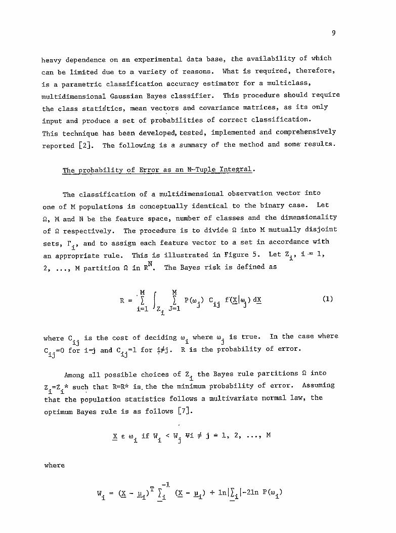
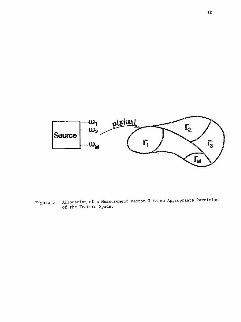
The classification of a multidimensional observation vector into
one of M populations is conceptually identical to the binary case Let
0 M and N be the feature space number of classes and the dimensionality
of Q respectively The procedure is to divide 2 into M mutually disjoint
sets Pi and to assign each feature vector to a set in accordance with -
an appropriate rule This is illustrated in Figure 5 Let Zi i = 1
2 M partition S1in R The Bayes risk is defined as
R = i J P(m) Ci f-Xlw) dX 1~ Z J=l
I
is the cost of deciding w1 where w is true In the case where
C=0 for ij and C=1 for ij R is the probability of error iJ 1
where C 13 i1
Among all possible choices of Z the Bayes rule partitions Q into1
Z=Z such that R=R is the the minimum probability of error Assuming1 1
that the population statistics follows a multivariate normal law the
optimum Bayes rule is as follows [7]
X a W3 if W lt W Vi j - 1 2 M
where
Wi = (X- i)T [i-1 (X-_u + ln[iZ-21n P(o)m
i0
~wo2 ~~WM
Allocation of a Measurement Vector X to an Appropriate Partition
F-igure5 of the Feature Space
with
X = observation vector
= mean vector for class w (2)
= covariace matrix for class 1
P( i) = apriori probability for i
The error estimate based on direct evaluation of Eq (1)exhibits all the
desired-properties outlined previously
The evaluation of multiple integrals bears little resemblance to
their one dimensional counterparts mainly due to the vastly different
domains of integration Whereas there are three distinct regions in one
dimension finite singly infinite and double infinite in an N dimensional
space there can potentially be an infinite variation of domains The
established one dimensional integration techniques therefore do not
carry over to N dimensions in general Hence it is not surprising that
no systematic technique exists for the evaluation of multivariate integrals
except for the case of special integrands and domains [8] The major
complicating factor is the decision boundaries defined by Eq (2) P is
defined by a set of intersecting hyperquadratics Any attempt to solve
for the coordinates of intersection and their use as the integration limits
will be frustrated if not due to the cumbersome mathematics because of
impractically complicated results
In order to alleviate the need for the precise knowledge of boundary
locations and reduce the dimensionality of the integral a coordinate
transformation followed by a feature space sampling technique is adopted
The purpose of the initial orthogonal transformation of the coordinates
is an N to 1 dimensionality reduction such that the N-tuple integral is
reduced to a product of N one dimensional integrals Let the conditional
classification accuracy estimate Pc be the desired quantity Then
the transformed class w statistics is given by
12
j = 1 2 M (3)
-3-S = 0T 0
where 0 is the eigenvector matrix derived fromi Naturally in each
transformed space Ti(Q) wi has a null mean vector and a diagonal
covariance matrix
The discrete feature space approach is capable of eliminating the
If 0 is theneed for the simultaneous solution of M quadratic forms
continuous probability space a transformation Ti is required such that
can be completely described in a nonparametric form therebyin TiQ) r1 1
bypassing the requirement foran algebraic representation of P This
desired transformation would sample Q into a grid of N-dimensional
hypercubes Since the multispectral data is generally modeled by a
multivariate normal random process a discrete equivalent of normal
random variables that would exhibit desirable limiting propertiesis
Let ynBi (n p) be a binomial random variable with parametersrequired
n and p The x defined by
Yu- npx Yn 0i 2 n (4)
converges to xN(O 1) in distribution [91 ie
lim F (X) - - F(x)n
The convergence is most rapid for p= then
(yn - n2)2 (5)n
13
The variance of xn is set equal to the eigenvalueof the transformed Yi by incorporating a multiplicative factor in Eq (5)
The segmentation of b a union of elementary hypercubes makes
nonparametric representation of P and its contours feasible Following1
the orthonormal transformation on o and sampling of 2 accordingly each1
cells coordinate is assigned to an appropriate partition of r This
process is carried outexhaustively therefore FI can be defined as a set
such that
r = ux x eli (6)
once the exhaustive process of assignment is completed the integral of
f(Xjwi) over Fi is represented by the sum of hypervolumes over the
elementary cells within P The elementary unit of probability is given by1
61 62 6N
f f (Xi) = 2 f (xli i ) dN T f (x 2 lo i ) d 2 2--2 f (xNIwi) dN
C -61 62 -N
2 2 2 (7)
where C is the domain of a sampling cell centered at the origin and 6
is the width of a cell along the ith feature axis The conditional
probability of correct classification is therefore given by
c Il+ 61 c2+ 62
Pcli - T (x i (x-l2) (C)dx2J f jw) (C)dx x c -6 2c -61
2 2
(8)
c +6 n n
c 2-- f (xNIwplusmn) II(C) dxN
c -6 n n
2
with overall classification accuracy given by
14
M
p P(m) P 1W (9)bullC I
where
1 if Cc (10)ii(C) =
0 otherwise
C = The domain of an elementary cell
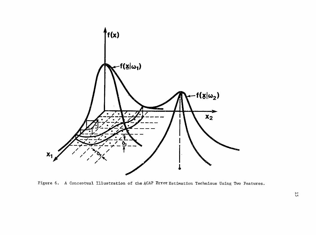
Figure 6 is a geometrical representation of Eq (8)
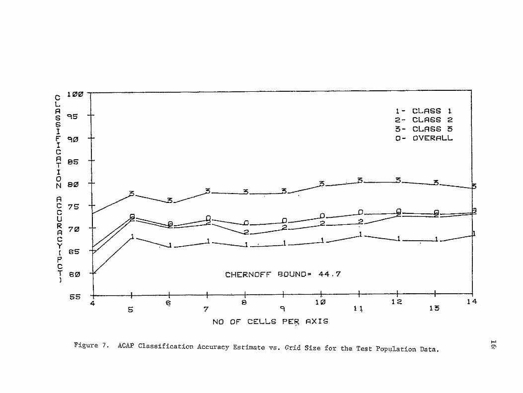
Experimental Results
The analytic classification accuracy prediction (ACAP) has been
Two examples are repeated hepethoroughly tested and documented [2]
The first experiment investigates the performance of the estimator vs
Small to moderate range ofgrid size ie number of cells per axis n
Figure 7 n is required if computation time is to remain realistic
vs n for three classes having some hypotheshyshows the variation of Pcjw c1
The main property of the estimator istical statistics in 3 dimensions
its rapid convergence toward a steady state value thereby alleviating
the need for excessively fine grids and hence high computation costs
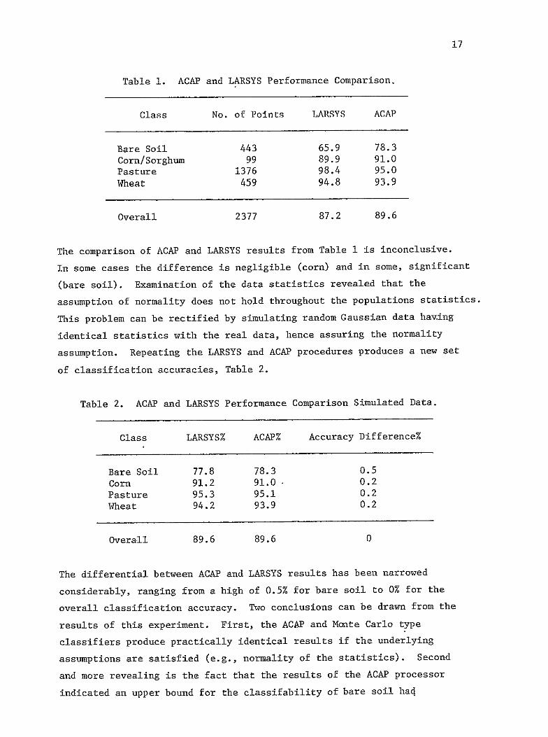
The data collected over Graham County Kansas is used to perform
a comparison between the ACAP algorithm and a ratio estimator such as
LARSYS The results are tabulated in Table 1
ff(x)
f(x~lQl)
xl
Figure 6 A Concentual
Illustration of the ACAP Error Estimation
Technicxue Using
Two Features FIEU
100C L A 1- CLASS I s -- 2- CLASS 2S
3- CLASS 51 r 110 0- OVERALL I CA as T I A
C 7S
C
PC
T So CHERNOFF BOUND- 447
ss tI1II
4 8 10 12 14S 7 9 11 15
NO OF CELLS PER RXIS
Figure 7 ACAP Classification Accuracy Estimate vs Grid Size for the Test Population Data 9
17
Table 1 ACAP and LARSYS Performance Comparison
Class No of Points LARSYS ACAP
Bare Soil 443 659 783
CornSorghum 99 899 910
Pasture 1376 984 950
Wheat 459 948 939
Overall 2377 872 896
The comparison of ACAP and LARSYS results from Table 1 is inconclusive
In some cases the difference is negligible (corn) and in some significant
(bare soil) Examination of the data statistics revealed that the
assumption of normality does not hold throughout the populations statistics
This problem can be rectified by simulating random Gaussian data having
identical statistics with the real data hence assuring the normality
assumption Repeating the LARSYS and ACAP procedures produces a new set
of classification accuracies Table 2
Table 2 ACAP and LARSYS Performance Comparison Simulated Data
Class LARSYS ACAP Accuracy Difference
Bare Soil 778 783 05
Corn 912 910 - 02
Pasture 953 951 02
Wheat 942 939 02
Overall 896 896 0
The differential between ACAP and LARSYS results has been narrowed
considerably ranging from a high of 05 for bare soil to 0 for the
overall classification accuracy Two conclusions can be drawn from the
results of this experiment First the ACAP and Monte Carlo type
classifiers produce practically identical results if the underlying
assumptions are satisfied (eg normality of the statistics) Second
and more revealing is the fact that the results of the ACAP processor
indicated an upper bound for the classifability of bare soil had
18
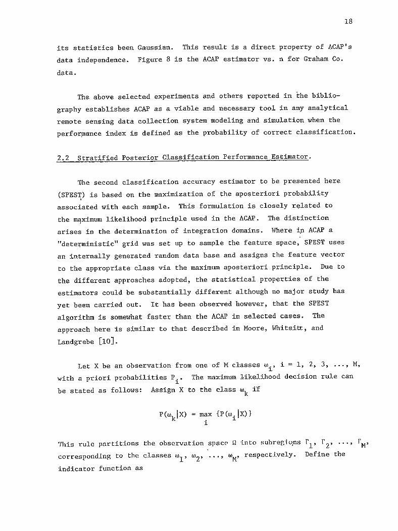
its statistics been Gaussian This result is a direct property of ACAPs
data independence Figure 8 is the ACAP estimator vs n for Graham Co
data
The above selected experiments and others reported in the biblioshy
graphy establishes ACAP as a viable and necessary tool in any analytical
remote sensing data collection system modeling and simulation when the
performance index is defined as the probability of correct classification
22 Stratified Posterior Classification Performance Estimator
The second classification accuracy estimator to be presented here
(SPEST) is based on the maximization of the aposteriori probability
associated with each sample This formulation is closely related to
the maximum likelihood principle used in the ACAP The distinction
arises in the determination of integration domains Where in ACAP a
deterministic grid was set up to sample the feature space SPEST uses
an internally generated random data base and assigns the feature vector
to the appropriate class via the maximum aposteriori principle Due to
the different approaches adopted the statistical properties of the
estimators could be substantially different although no major study has
yet been carried out It has been observed however that the SPEST
algorithm is somewhat faster than the ACAP in selected cases The
approach here is similar to that described in Moore Whitsitt and
Landgrebe [10]
1 2 3 MLet X be an observation from one of M classes wi i =
with a priori probabilities P The maximum likelihood decision rule can 1
be stated as follows Assign X to the class w k if
P(ikIX) = max P(wiX)JX) i
This rule partitions the observation space Q into subregions FI 12 PM
corresponding to the classes il ()2 M respectively Define the
indicator function as
C 100-U
A
4 - - - 4 - - 4 - 4 - -- 4 - - -S4 ~_ ---- 4- --- -4
FI ~~~
N 4
R C I- CLASS 1 C 2- CLASS 25- CLRSS 5 R 4- CLASS 4 C 0- OVERRLL Y
PSC
T ) 1
7S I I 4 8 10 12 14 16
s 7 9 11 15 15 17
NO Or CELLS PER RXIS
Figure 8 ACAF Classification Accuracy Estimate vs Grid Size for Graham Co Kansas Data
kH
20
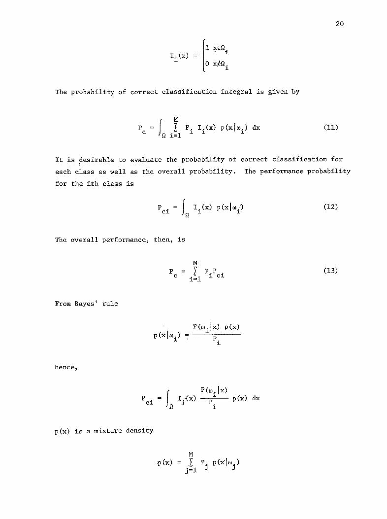
The probability of correct classification integral is given by
Pc = f M I(x) p(xi) dx (11)
It is desirable to evaluate the probability of correct classification for I
each class as well as the overall probability The performance probability
for the ith class is
Pci = JI i(x) p(xltamp (12)
The overall performance then is
M
p = iPci (13) c i= l1 c
From Bayes rule
P(mijx) p(x)
p(xli) P
hence
Pci = l(x) ptn p(x) dx
p(x) is a mixture density
M
p(x) = X P pjx jl p (
21
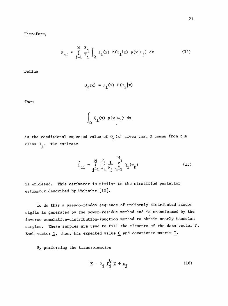
Therefore
M P
I - T2 x) P(4)Ix) p(xV1 ) dx (14)Pc1 j=l P i (
Define
Qi(x) = Ii(x) P((i Ix)
Then
f Qi(x) p(xIW) dx
is the conditional expected value of Qi(x) given that X comes from the
class C The estimate
M p N
(15)j=l PN I Qi(xk)j=P5 jJ k=l
is unbiased This estimator is similar to the stratified posterior
estimator described by Whitsitt [10]
To do this a pseudo-random sequence of uniformly distributed random
digits is generated by the power-residue method and is transformed by the
inverse cumulative-distribution-function method to obtain nearly Gaussian
samples These samples are used to fill the elements of the data vector Y
Each vector Y then has expected value 0 and covariance matrix I
By performing the transformation
X = F Y + m (16)J j - -3
22
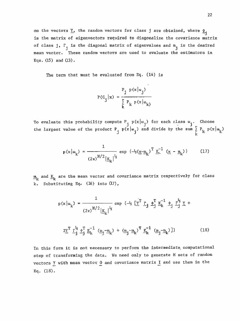
On the vectors I the random vectors for class j are obtained where 4
is the matrix of eigenvectors required to diagonalize the covariance matrix
of class j rS is the diagonal matrix of eigenvalues and m is the desiredJ
These random vectors are used to evaluate the estimators in mean vector
Eqs (15) and (13)
The term that must be evaluated from Eq (14) is
P p(xlwo)
P(CIx) = YPk P(X_ k Q
k
To evaluate this probability compute P p(xloj) for each class w Choose
the largest value of the product P p(xlm) and divide by the sum P P(XLk)j k
P(x~mk) = exp - (x-mk)T K1 (x - m) (17)
(27F) 2K I
and Kk are the mean vector and covariance matrix respectively for class
k Substituting Eq (16) into (17)
p(xIk) = - exp - T T- Y
2YT r T -1 1 -18 -2 -j Kk (-m-mk) 4 (m-mk) K (m-mk)] (18)
In this form it is not necessary to perform the intermediate computational
step of transforming the data We need only to generate M sets of random
vectors Y with mean vector 0 and covariance matrix I and use them in the
Eq (18)
23
Estimator Evaluation
A subroutine program was written to evaluate classification perforshy
mance by the above method To test the method a three class problem was
constructed The mean vectors for the classes were
1 ]T
S = [-i -i ]T M 2 [0 0
N2 T L3 = [ ]
The covariance for each class was the identity matrix The number of
random vectors generated for each class was 1000 The exact classificashy
tion accuracy as a functidn of the dimensionality can be evaluated for
this case
P = 1 - erfc (fi2)
Pc2 = 1 - 2 erfc (VN2)
P = 1 - erfc (A-2)
P =1 - 43 erfc (AT2)c
t~ -X22
where erfc (a) = edx
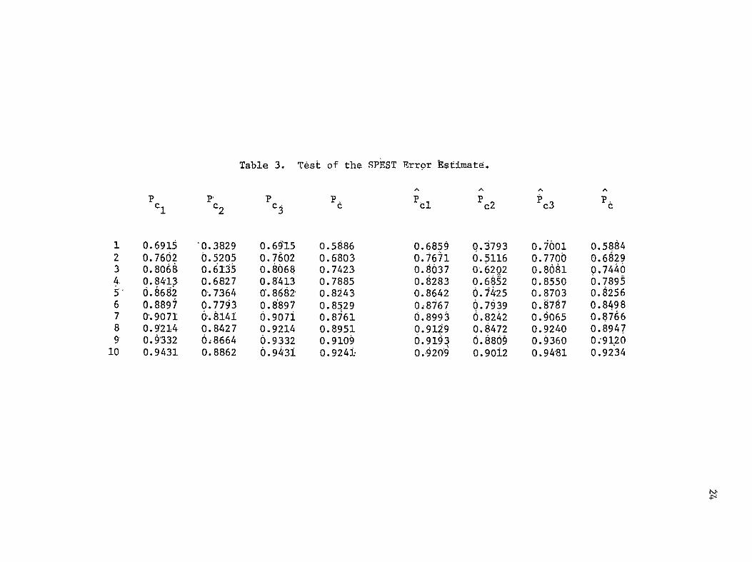
and n is the number of dimensions Table 3 contains the results of
evaluating the class conditional performance and overall performance
from one to ten dimensions
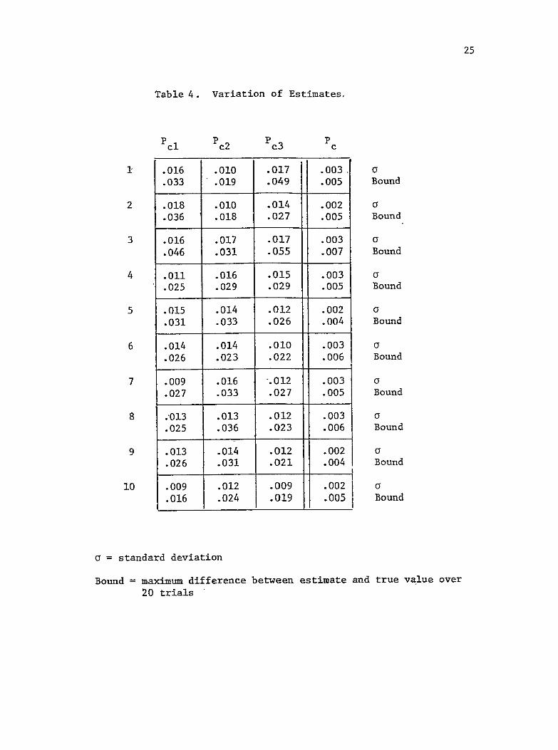
To evaluate the variance of the estimates different starting values
for the random number generator were used Twenty trials were used to
evaluate the maximum bound and the standard deviation from the true value
These results are presented in Table 4
For the overall accuracy the estimate is within 005 of the true
value This is certainly sufficient for performance estimation The
Table 3 Test of the SPEST Error Estimatd
Pc1c P P P Pc2 Pc30
1 06915 03829 06q15 05886 06859 03793 07001 05884 2 07602 05205 07602 06803 07671 05116 07700 06829 3 08068 0613j5 08068 07423 08037 06202 08081 07440 4 084-13 06827 08413 07885 08283 06852 08550 07895 5 08682 0-7364 08682 08243 08642 07425 08703 08256 6 08897 07793 08897 08529 08767 07939 08787 08498 7 09071 0814I 0907i 08761 08993 08242 09065 08766 8 09214 08427 09214 08951 09129 08472 09240 08947 9 09332 68664 09332 09109 09193 08809 09360 09120
10 09431 08862 6943i 0924i 09209 09012 09481 09234
25
Table 4 Variation of Estimates
pcl Pc2 Pc3 Pc
1 016 010 017 003 a 033 019 049 005 Bound
2 018 010 014 002 a 036 018 027 005 Bound
3 016 017 017 003 C
046 031 055 007 Bound
4 011 016 015 003 a 025 029 029 005 Bound
5 015 014 012 002 a 031 033 026 004 Bound
6 014 014 010 003 a 026 023 022 006 Bound
7 009 016 012 003 a 027 033 027 005 Bound
8 013 013 012 003 025 036 023 006 Bound
9 013 014 012 002 a 026 031 021 004 Bound
I0 009 012 009 002 a 016 024 019 005 Bound
a = standard deviation
Bound = maximum difference between estimate and true value over 20 trials
26
class conditional estimates are less reliable but are sufficient to
observe trend in the performance due to individual classes
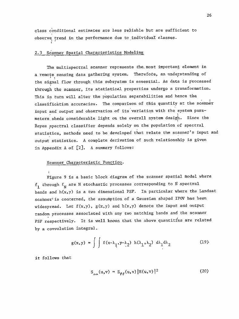
23 Scanner Spatial Characteristics Modeling
The multispectral scanner represents themost important element in
a remote sensing data gathering system Therefote an understanding of
the signal flow through this subsystem is essential As data is processed
through the scanner its statistical properties undergo a transformation
This in turn will alter the population separabilities and hence the
classification accuracies The comparison of this quantity at the scanner
input and output and observationof its variation with the system parashy
meters sheds considerable light on the overall system design Since the
Bayes Ppectral classifier depends solely on the population of spectral
statistics methods need to be developed that relate the scanners input and
output statistics A complete derivation of such relationship is given
in Appendix A of [2] A summary follows
Scanner Characteristic Function
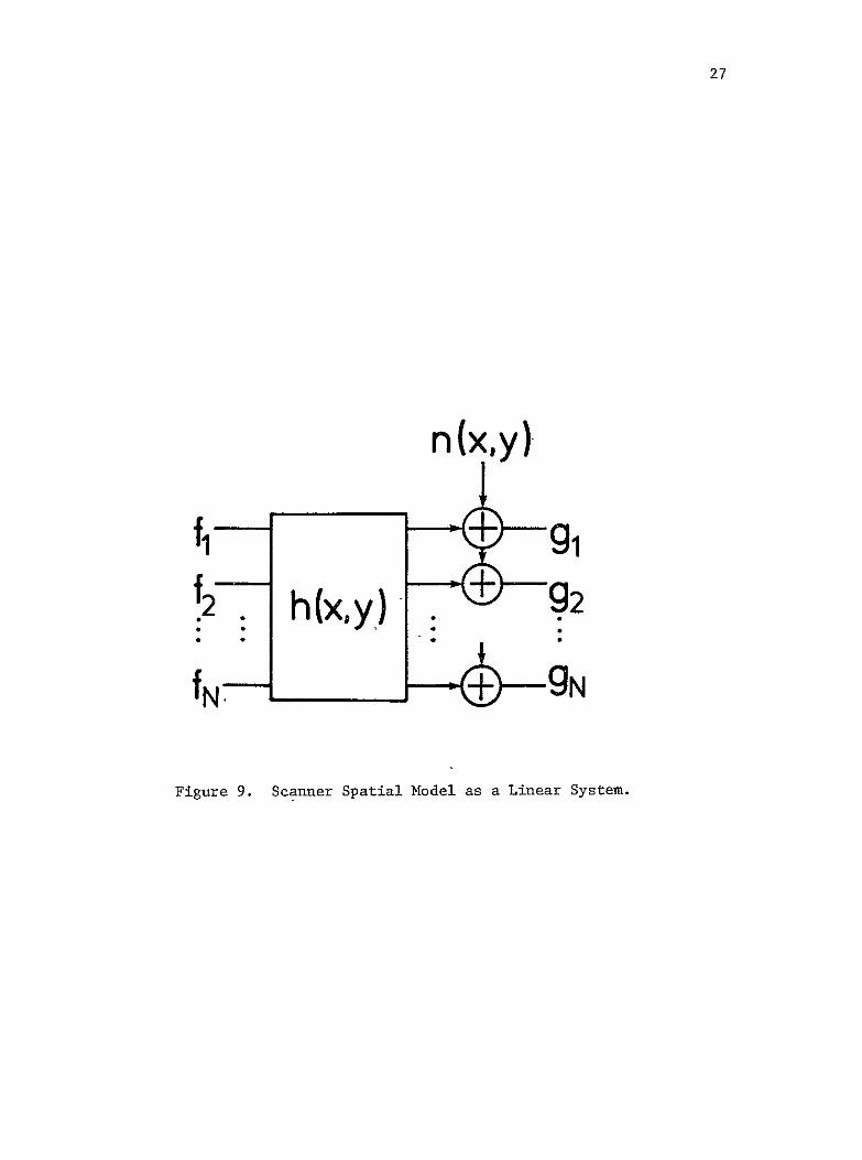
Figure 9 is a basic block diagram of the scanner spatial model where
f through fN are N stochastic processes corresponding to N spectral
bands and h(xy) is a two dimensional PSF In particular where the Landsat
scanner is concerned the assumption of a Gaussian shaped IFOV has been
widespread Let f(xy) g(xy) and h(xy) denote the input and output
random processes associated with any two matching bands and the scanner
PSF respectively It is well known that the above quantitfes are related
by a convolution integral
Jg(xy) f f(x-1y-A 2 ) h(XV1 2) d IdX 2 (19)shy
it follows that
S(UV) SIf(uv)IH(uv)l2 (20)
27
n(xy)
f2 h(xy)+ 92
f- _-+ gN
Figure 9 Scanner Spatial Model as a Linear System
28
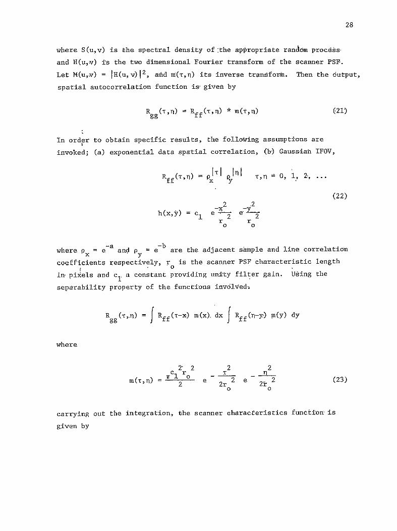
where S(uv) is the spectral density of the appropriate random process
and H(uv) is the two dimensional Fourier transform of the scanner PSF
Let M(uv) = IH(uv)12 afd m(Tn) its inverse transform Then the output
spatial autocorrelation function is given by
R (Tn) = Rff(Tn) m(Tn) (21)
In order to obtain specific results the following assumptions are
invoked (a) exponential data spatial correlation (b) Gaussian IFOV
PIT I Rff(Tn) = 011 rn 0 1 2
(22)
2 2 h(xy) = c1 e - e2
r r 0 0
=-a =-b where px = e and py = e are the adjacent sample and line correlation
coefficients respectively r is the scanner PSF characteristic length
O in-pixels and c1 a constant providing unity filter gain Using the
separability property of the functions inv6lvedi
R g(TI) = Rff(T-X-) m(x) dx f Rff((Th-y) rn(y) dyJ where
c 2 2 r0 2 2 n
m(rr) = 2 e 2r 2e 2- 2 (23)
0 0
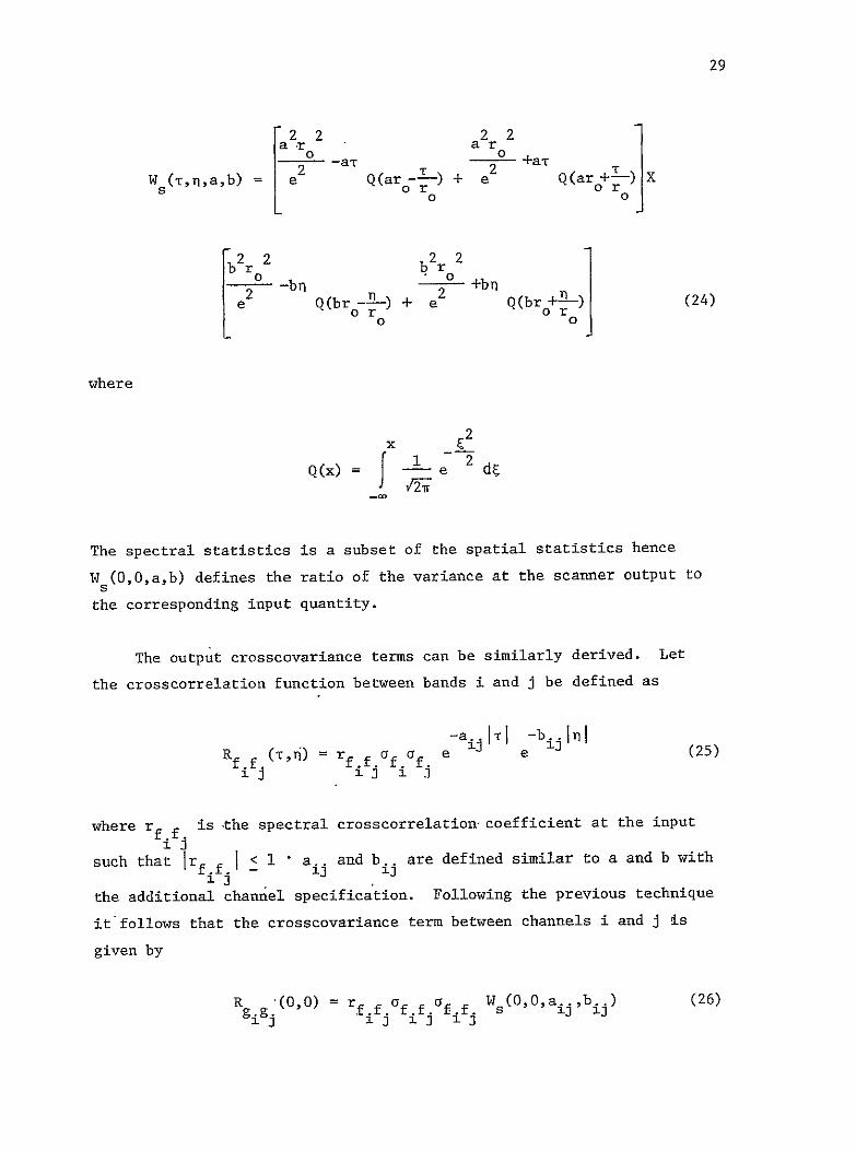
carrying out the integration the scanner characteristics funation is
given by
29
2 a222 lar a r
_- -aT +a
W (TIab) = Q(ar --L-) + e Q(ar +U)X 0 0
bt~rr 2or Qb l
o + o +bf
2Lr- Q(br2Q(br ) (24)e
where
2x
Q(x) = e 2
The spectral statistics is a subset of the spatial statistics hence
W (00ab) defines the ratio of the variance at the scanner output to s
the corresponding input quantity
The output crosscovariance terms can be similarly derived Let
the crosscorrelation function between bands i and j be defined as
Rff (T) = rffaf of e-aeIrI -biiI (25)213 1J 1 j
where rf f is the spectral crosscorrelation-coefficient at the input
such that Irff I lt 1 aij and bIj are defined similar to a and b with
the additional channel specification Following the previous technique
it follows that the crosscovariance term between channels i and j is
given by
Rggj (00) = rffoff off Ws(00aijb)ij (26)
1J 1 J i i ij 12 2
30
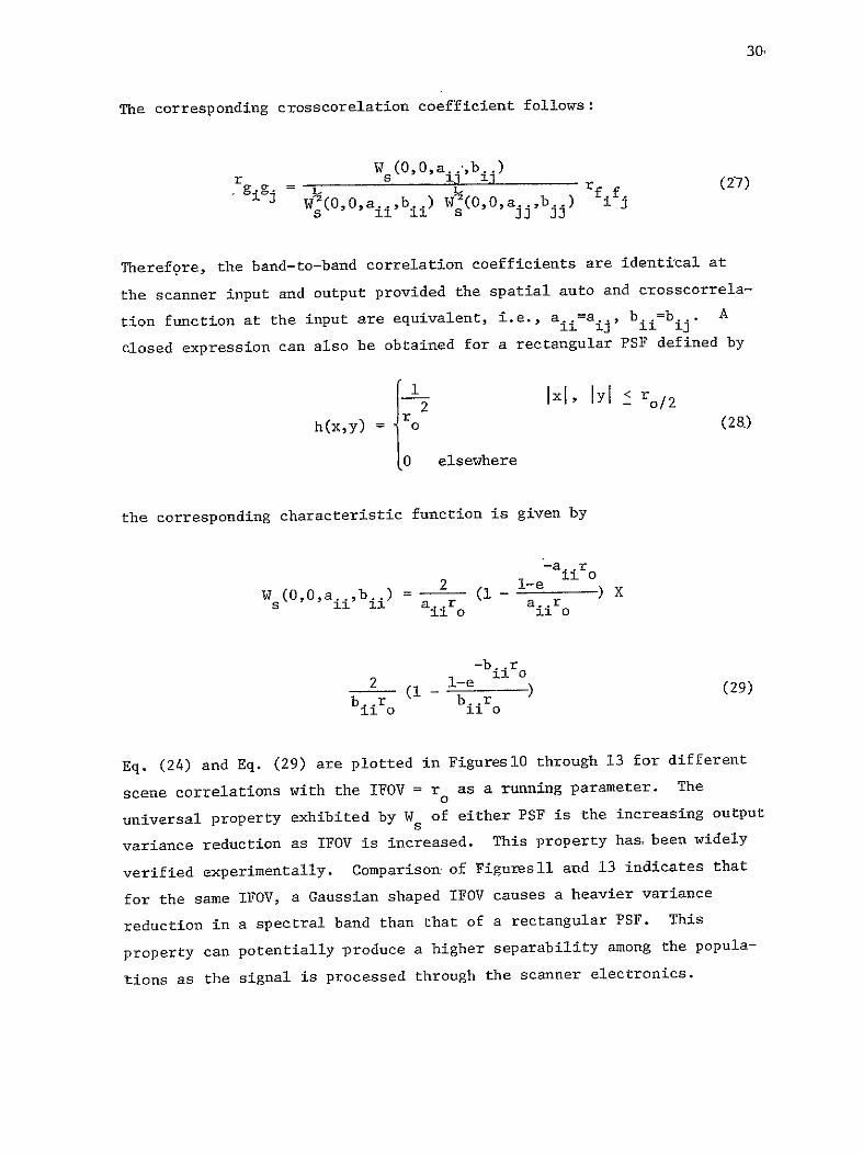
The corresponding crosscorelation coefficient follows
W (00a ibi) Sgigj - rff
w 2(00aii~bii) WbOOa b) i s si 33 33
Therefore the band-to-band correlation coefficients are identical at
input and output provided the spatial auto and crosscorrelashythe scanner
tion function at the input are equivalent ie aiiaij biib ij A
closed expression can also be obtained for a rectangular PSF defined by
I~o Ix lyl o2
(28)h(xy) =
0 elsewhere
the corresponding characteristic function is given by
-a r
(i1 - ) X -lW (OOa)= 2 l-e 110
s O aiii ar ar I 0 11 0
-br
br2 (I l-er 110 -) (29)
ii o ii 0
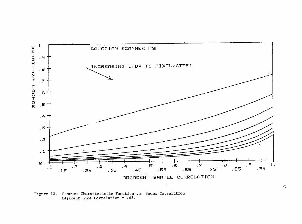
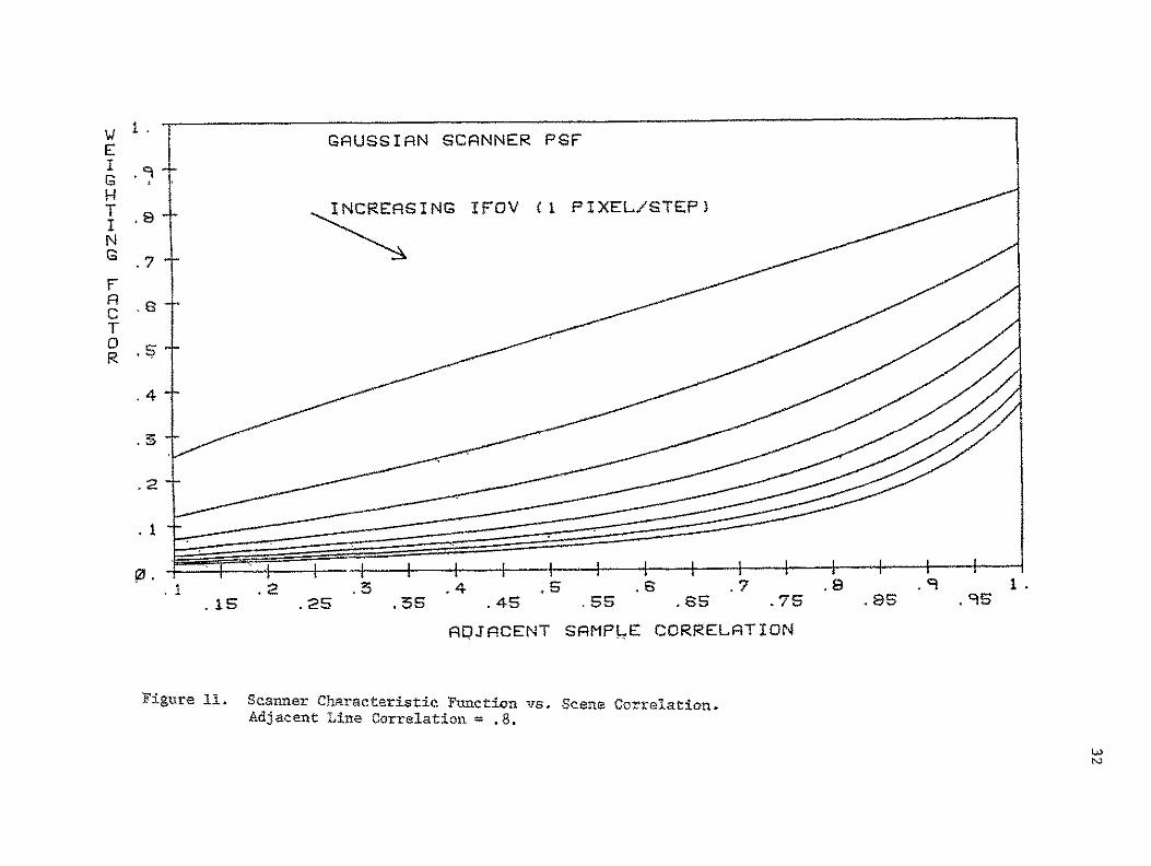
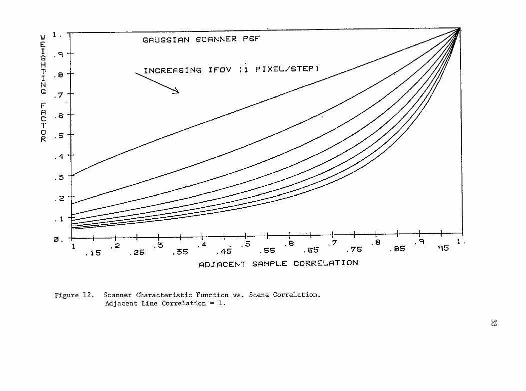
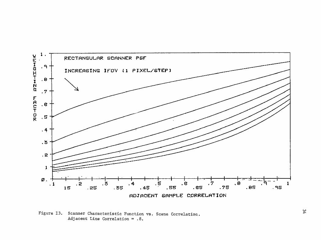
Eq (24) and Eq (29) are plotted in Figures10 through 13 for different
as a running parameter The scene correlations with the IFOV = r0
of either PSF is the increasing outputuniversal property exhibited by Ws
variance reduction as IFOV is increased This property hasbeen widely
verified experimentally Comparison of Figumsll and 13 indicates that
for the same IFOV a Gaussian shaped IFOV causes a heavier variance
a rectangular PSFreduction in a spectral band than that of This
property can potentially produce a higher separability among the populashy
tions as the signal is processed through the scanner electronics
W 1 GAUSSIAN SCANNER PSF EI
H INCREASING IFOV (i PIXELSTEP)T 8
I N G7
F A C T0 R
2 2 N 8
0 1 is 2 6 5 5 5 4 5 s S 5 e 7 5 a s 96 95
ADJACENT SAMPLE CORRELATION
Figure 10 Scanner Characteristic Function vs Scene Correlation Adjacent Line Correlation = 65
W GOUSSIRN SCANNER PGF E I G H
N
T 8INCREASING IFOV (I PIXELSTEFP
C
R
FA
T0
04
1 15
2
2s
5S
4 8 4S 5 75
ROJPCENT SRMPE CORRELATION
8 85 S
Figure 11 Scanner Characteristic Function vs Scene Correlation Adjacent Line Correlation = 8
E 1 GRUSSIRN SCANNER PSF
H T8 I N G F A
INCREASING IFOV (1 PIXELSTEP)
T
R
4
2
1
1
15
2
25
5s
4 S 7
4S 55 8s 7S
ADJACENT SRMPLE CORRELATION
85
9 95
Figure 12 Scanner Characteristic Function vs Scene Correlation Adjacent Line Correlation = 1
1 RECTANGULAR SCNNER PSF
I 9 rINCREASINGH IFOV (I PIXELSTEP)
T I N G
F A C T 0
4
2
IA 2 4 68 7 8 1s 2S 5s 4S SS s 7S 85 9s
ADJACENT SANPLE QORRELATION
Figure 13 Scanner Characteristic Function vs Scene Correlation
Adjacent Line Correlation = 8
35
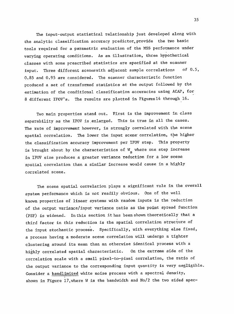
The input-output statistical relationship just developed along with
the analytic classification accuracy predictorprovide the two basic
tools required for a parametric evaluation of the MSS performance under
varying operating conditions As an illustration three hypothetical
classes with some prescribed statistics are specified at the scanner
input Three different sceneswith adjacent sample correlations of 05
085 and 095 are considered The scanner characteristic function
produced a set of transformed statistics at the output followed by the
estimation of the conditional classification accuracies using ACAP for
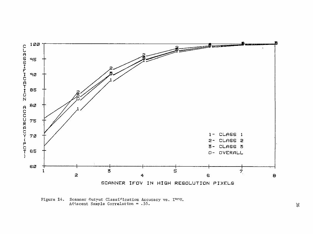
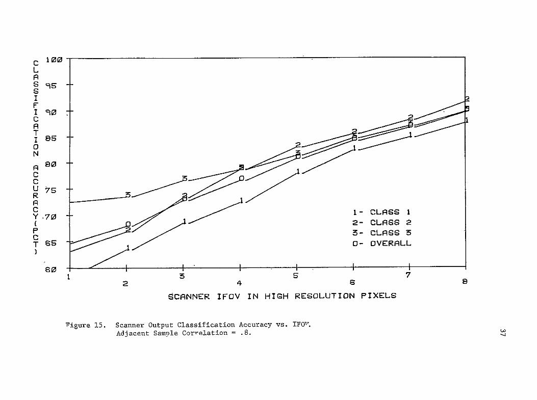
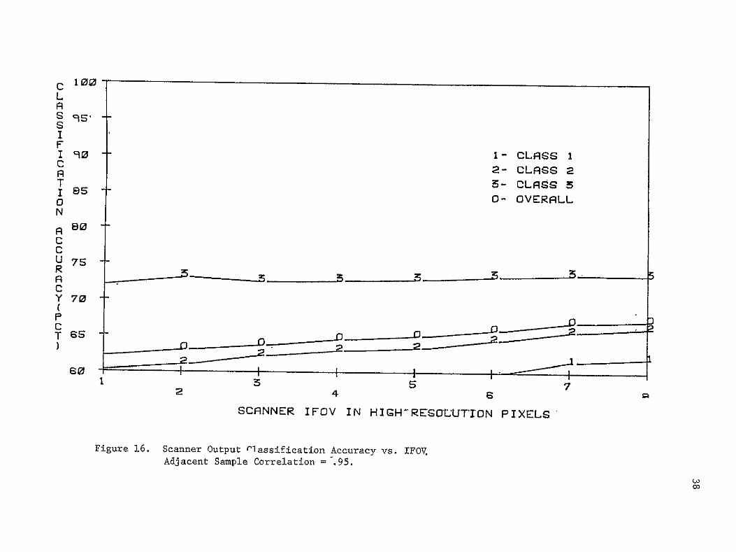
8 different IFOVs The results are plotted in Figuresl4 through 16
Two main properties stand out First is the improvement in class
separability as the IFOV is enlarged This is true in all the cases
The rate of improvement however is strongly correlated with the scene
spatial correlation The lower the input scene correlation the higher
the classification accuracy improvement per IFOV step This property
is brought about by the characteristics of Ws where one step increase
in IFOV size produces a greater variance reduction for a low scene
spatial correlation than a similar increase would cause in a highly
correlated scene
The scene spatial correlation plays a significant role in the overall
system performance which is not readily obvious One of the well
known properties of linear systems with random inputs is the reduction
of the output varianceinput variance ratio as the point spread function
(PSF) is widened In this section it has been shown theoretically that a
third factor in this reduction is the spatial correlation structure of
the input stochastic process Specifically with everything else fixed
a process having a moderate scene correlation will undergo a tighter
clustering around its mean than an otherwise identical process with a
highly correlated spatial characteristic On the extreme side of the
correlation scale with a small pixel-to-pixel correlation the ratio of
the output variance to the corresponding input quantity is very negligible
Consider a bandlimited white noise process with a spectral density
shown in Figure 17where W is the bandwidth and No2 the two sided specshy
0 1001
I go
C Rq T S86
N
P8r C C U 7 153 R R C Yr 70
1
I1- CLSSS
2- CLRSS
I
C T 85
3-0-
CLRSS 5 OVERRUL
SCFRNNER IFOV IN HIGH RESSLUTION PIXELS
Figure 14 Scanner Output Classification Accuracy vs Ifl Adiacent Sample Correlation = 55w
C 100
L R S I F
Ao
T1 85
0 N
8 0f1C C U 75 R C I- CLASS I Y 70
2- CLASS 2 F 3- CLASS 5C
0- OVEWILLT BE
742
SCANNER IFOV IN HICH RESOLUTION PIXELS
7Figure 15 Scanner Output Classification Accuracy vs IFONAdjacent Sample Correlation = 8
10c LAS 9- O SI F
CC 2- CLASS 2
1 85 T 3- CLA~SS 5 0 0- OVERALL
N
A80 C
UR
C 7S
C Y 70
P
T GS
2 4 8
SCRNNER IFOV IN HIGH-RESCUTION PIXELS
Figure 16 Scanner Output Classification Accuracy vs IFOV Adjacent Sample Correlation = 95
00
39
No2
-2gW 27W w
Figure 17 Bandlimited White Noise Spectral Density
tral density As W increases the adjacent pixel correlation in the
scene decreases The increase in W however is accompanied by a
decrease in No2 if this process is to remain physically realizable
(finite energy) Under a finite energy constraint therefore as W-shy
No2-- 0 In the limit the energy content of the output random process
will be nil
Random Noise
Additive random noise entered at various stages of a scanner system
can degrade the overall system performance substantially The noise can
be classified into two broad categories external and internal A
major source of external noise is atmospheric in nature mainly due to
absorption (eg water vapor) and scattering The detector and quantishy
zation noise comprise the major component of the internal noise sources
From a system analysis point of view the latter represents a more tractshy
able and better understood component of the random noise [11] while
the former still awaits further experimental documentation The purpose
of this work is not so much the exploration of the various noise sources
but the integration of its effect within an analytic analysis package
once its characteristics and origin has been determined
can be stated that atmosphericFrom the theoretical results obtained it
noise in the uplink path at least has negligible degrading factor
compared with the detector and quantization noise Let f(xy) Nf(xy)
f(xy) and Nf(xy) be the input random process input additive white
40
noise the output random process and the noise component of the output
signal respectively then
f-(xy) = f(xy) h(xy) (30)
N (xy) = Nf(xy) h(xy) (31)f
Define
(SNR)f = Var f(xy)1Var Nf(xy)l (32)
(SNR) -= Var f(xy)Var N (xy)) (33) f f
Recalling the functional dependence of Ws on the input scene spatial
correlation it follows that the ratio of the variance of a white noise
process at the scanner output to the corresponding input quantity is of
the order of 5 to 10 higher or lower depending on the IFOV size
Therefore
Var f(xy) lt Var f(xy)l (34)
Var N (xy)l ltlt Var Nf(XY (35)f
hence
(SNR) f gtgt (SNR)f (36) f
It then follows that the noise component of the output process prior to
casesdetector and quantization noise is negligible in most
In order to observe the effect of noise on the scanner output class
separability the test class statistics were modified to exhibit the effect
of random noise The assumed properties of the noise are additive
white and Gaussian Let F-(xy) )e the signal to be teJmeterud to
Earth
41
f(xy) = f(xy) + N (xy) (37) f
the statistics of f(xy) and f(xy) are related by
+ Y (38) r~f -N
f
the simple addition is due to the signal and noise independence Assuming
a zero mean N the mean vector are identical ie f
E ffj = E f-)
Among the four assumptions about the noiseits Gaussian property is the
weak link due to the Poisson distributed detector noise and uniformly
distributed quantization noise Relaxing the Gaussian noise assumption
however would mean the design of an optimum classifier for non-normal
classes and evaluation of its performance A task that would complicate
matters considerably Due to the relatively insufficient documentation
of the characteristics of random noise in multispectral data the initial
Gaussian assumption is adhered to
Following the adopted SNR definition three different noise levels
are considered and the corresponding overall classification accuracies
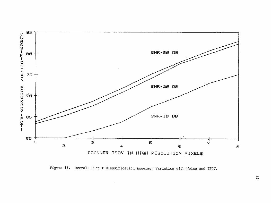
for the three previously used test classes are estimated Figure 18 is
the variation of P vs IFOV with SNR as the running parameter For a c
fixed IFOV P increases with increasing SNR For a fixed SNR P c c
increases with increasing IFOV size These illustrations have shown
that with a proper coupling between the ACAP and the scanner characteristic
function the progress of the population statistics through the system
can be studied on an analytical and entirely parametric basis The
accompanying classification accuracies can measure the designers success
in selecting the spatial andor spectral characteristics of a Multispectral
Scanner System
C S LSs
1 80 SNR-50 0BF 8 I C R
I 7 -0 N
T
37cent0 U
C
R
C Y ( 6s-- SNR=10 0B P 6 C T
2 4 6
SCANNER IFOV IN HIGH RESOLUTION PIXELS
Figure 18 Overall Output Classification Accuracy Variation with Noise and IFOV
43
24 Optimum Spectral Function Research
In earth observational remote sensing much work has been done with
extracting information from the spectral variations in the electromagnetic
energy incident on the sensor Of primary importance for a multispectral
sensor design is the specification of the spectral channels which sample
the electromagnetic spectrum An analytical technique is developed for
designing a sensor which will be optimum for any well-defined remote
sensing problem and against which candidate sensor systems may be compared
Let the surface of the earth at a given time be divided in strata
where each stratum is defined to be the largest region which can be
classified by a single training of the classifier Each point in the
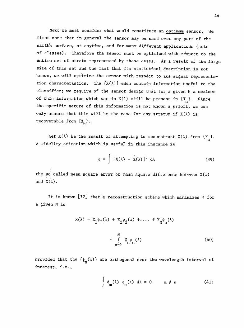
stratum is mapped into a spectral response function X(X) as in Figure 19
That is if one observes a point in the stratum with the sensor then the
function X(A) describes the response variations with respect to the
wavelength X The stratum together with its probabilistic description
defines a random process and the collection of all of such functions
X(X) which may occur in the stratum is called an ensemble
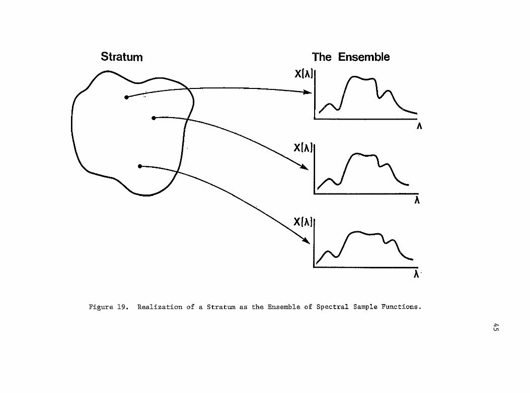
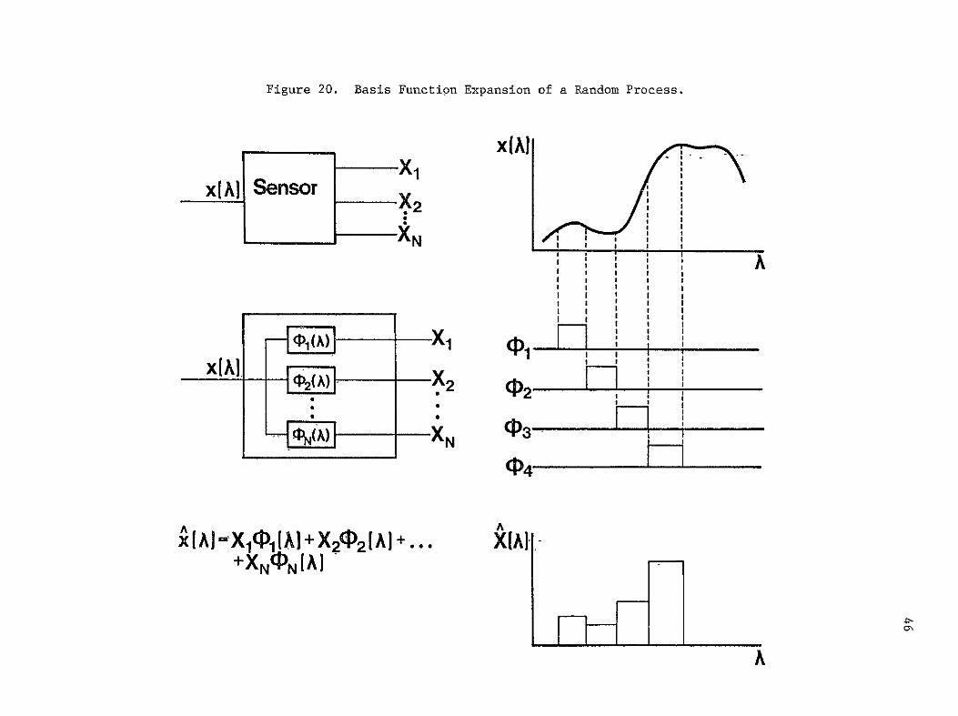
The general concept of a pattern recognition system in this applicashy
tion requires that if each X(X) is to be classified by a classification
algorithm this can be accomplished by first measuring a finite number
of attributes of X(A) called features This is the function of the
sensor system as depicted in the upper left portion of Figure 20 where
X1 X2 X are the values of N features for a given X(X) It
may be viewed as a filtering operation on X(A)
For example on the right portion of Figure 20 the function of MSS
of the Landsat satellites is illustrated In this case a number proporshy
tional to the average energy in a wavelength interval is reported out by
the sensor for each of four wavelengths Mathematically this may be
expressed as
Zn f X n)(X)dX n = 1 2 3 4
44
Next we must consider what would constitute an optimum sensor We
first note that in general the sensor may be used over any part of the
earthb surface at anytime and for many different applications (sets
of classes) Therefore the sensor must be optimized with respect to the
entire set of strata represented by these cases As a result of the large
size of this set and the fact that its statistical description is not
known we will optimize the sensor with respampct to its signal representashy
tion characteristics The fX(A) each contain information Useful to the
classifier we require of the sensor design that for a given N a maximum
of this information which was in X(A) still be present in X Since n the specific nature of this information is not known a priori we can
only assure that this will be the case for any stratum if X(A) is
recoverable from fX I n
Let X(A) be the result of attempting to reconstruct X(A) from X n
A fidelity criterion which is useful in this instance is
= f[X(X) - x(X)] 2 dA (39)
the so called mean square error or mean square difference between X(X)
and X(A)
It is known [12J thata reconstruction scheme which minimizes C for
a given N is
X(A) = XI1 (A) + X2 2(A)+ + +n(A)
N X + (A) (40)
n=l
provided that the n(A) are orthogonal over the wavelength interval of
interest ie
S m(X)n(X) d) = 0 m n (41)
Stratum The Ensemble
A
A
A
Figure 19 Realization of a Stratum as the Ensemble of Spectral Sample Functions
Figure 20 Basis Function Expansion of a Random Process
x(AxSensorI X2
XN
A A
I
I
I
I-- i
X1lA) =Xl~il l +X2I2A]I+
4SNA)
^
47
and the X are calculated byn
X = X(x) Mn(3dA (42)
Note for example thatthe Landsat example of Figure 20 satisfies
these conditions In the lower right of Figure 20 is depicted the
result of such a reconstruction for the Landsat example
While use of Eq (42) in the case does minimize s with respect to
the choice of values of TX 1 a further improvement may by obtained byn
choosing a set of iIXI which minimizes E Itcan be shown [5 12]
that the set n(X) which accomplishes this must satisfy the equation
U = R(AC) C()dC (43)
where
R(XC) = E[X(A) - m()] [X( ) - m( )]1 (44)
is the correlation function of the random process and m(X) is its mean
value at X
Such a signal tepresentation defined by Eqs (40-44) is known as a
Karhunen-Lo~ve expansion [13] It provides not only for the most rapid
convergence of X(X) to X(X) with respect to N but in addition the random
variables (X are uncorrelated and since the random process is Gaussian n
they are statistically independent Further the only statistic required
of the ensemble is R(XC) This representation of X(X) is therefore
not only optimal it is convenient
A useful generalization of the Karhunen-Lo~ve expansion can be made
Suppose a priori information concerning portions of the spectral interval
are known and it is desired to incorporate-this knowledge into the analysis
A weighting function w(A) is introduced which weights portions of the
interval according to the a priori information As an example measureshy
48
ments were taken over the spectrum and it was observed that there was
considerable variation in the signal in the water absorption bands
around 14 and 18 micrometers This variation was due to measurement
and calibration difficulties rather than being a result of variations
in the scene Therefore the weighting function was set to zero in
these absorption bands This generalization is referred to as the
weighted Karhunen-Lo~ve expansion [5] Eqs (40) (42) and (43) become
N X(A) = x( AsA (45)
i=1l
a (A) = FR(AE) w( ) 4 (E)dE (46)w i f w
x X(A) w() tw (X) dA (47) 1
where the eigenfunction 41 (A) are solutions to the integral Eq (46)W 1
with the weight w(A) The special case where w(A) = 10 for all AcA
reduces the expansion to the original form in Eq (40) (42) (43) and
(44)
The results of having utilized this means of optimal basis function
scheme on spectral data are contained in reference [5] From them one car
see the significant improvement in classification accuracy which decreased
spectral representation error will provide One can also determine the
spectral resolution and band placement needed to achieve such classification
accuracy improvement
25 Information Theory Approach to Band Selection
The ptoblem of selecting a set of optimum windows in the electroshy
magnetic spectrum for observing the reflected sunlight has always been of
considerable interest Depending on the definition of the optimality
different methods have been developed One such approach was shown in
Section 24 using K-L expansion to select an optimum set of basis functions
In this section an information theoretic definition of optimality developed
in [3] is explored
49
Mutual Information and Stochastic Modeling
The reflected energy from the target is detected by the scanner
and corrupted by various noise sources If S is the noise-free signal
Y the observation and N a random disturbance then
Y = S + N (48)
the reduction of uncertainty about S obtained from Y is called the
average or mutual information between the observation and original signal
Since the reconstruction of the reflected signal from the noisy observashy
tion is the highly desirable capability the comparison of such average
information-and selection of these bands with the highest information
content is chosen as-a means of spectral band selection Let
S = (sl s 2 )
and
)Yn =(Yl Y2 Yn
where si and yi are the coefficients of the orthonormal (K-L) expansion
of Y and S then the mutual information between Y and S is given by [3]
T(YS) = - log et (49)
where C and C are the covariance matrices of (yi i = 1 2 ) and
(ni = No2 i = 1 2 ) and No2 is the two sided spectral density of
the additive white noise Equivalently I(YS) can be represented in
terms of the Wiener-Hopf optimum filter impulse response
A-(2
T()= J h(AA) dA (50)
11
50
h(XA) provides an estimate of S from Y with a minimum mean-square error
This relationship however is not a practic d-dethod of evaluating I(YS)
since the actual solution of the Wiener-Hopf integral itself is a nontriyal
task This problem can be circumvented by a discrete state variable
formulation ieshy
s(k+l) = _s(k) + FW(k) ke[Al x2 ] (51)
where
s1(k+l)
s2(k+l)
s(k+l) =
Sn(k+l)
is an (nxn) matrix
r is an (nxl) vector
W(k) = a descrete independent Gaussian
zero mean random process
The formulation of the problem in the discrete domain -provides a practical
way of computing hXX) through Kalman filtering techniques The discrete
version of Eq (50) is given by
I(YS) = - h(kk)
k 6 AA 2 (52)
The discrete nature of this approach makes the evaluation of Eq (52)
considerably more practical than its continuous counterpart This is due
to the fact that the Wiener-Hopf equation is easily solved in only those
cases for which the analytical form of Ks (Au) the signal eovariance
fnnction is fairly simple not likely for most-random processes encountered
51
in remote sensing Since h(kk) is dependent on the parameters of Eq (51)
a concise representation of s(k+l) is needed
The general form of Eq (51) is given as an autoregressive (AR)
model
m1 m2
s(k) = X as(k-j) + I bji(k-j) + W(k) (53) j=l J j1
s(k) = The spectral response at the discrete
wavelength k It is a Gaussian random process
w(k) = zero mean independent Gaussian disturbance
with variance p
(kj) = deterministic trend term used to account for certain characteristics of the empirical data
ab = are unknown constant coefficients to be I i determined
mlm2 = The order of the AR model
The identification selection and validation of general AR models
for the representation of a random process is a well developed technique
[1415] The identification of an appropriate model provides the
necessary parameters required for the evaluation of I(YS) in Eq (52)
The model selection process for a selected number of ground covers has
been carried out [3] leading to the ranking of a set of spectral bands
according to the criterion outlined previously A summary of the
experimental results are given below
Data Base and Model Selection
Two different sets of empirical data are used to demonstrate the
techniques developed here The first set consists of observations of
wheat scenes The second set consists of several vegetation cover
types such as oats barley grass etc For each scene the spectral
responses collected by the Exotech 20C field spectroradiometer are
averaged over the ensemble It is thought the resultant average
52
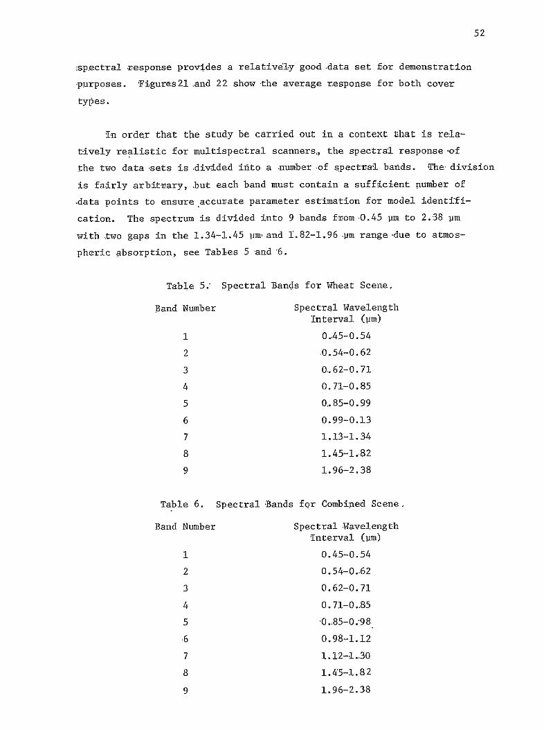
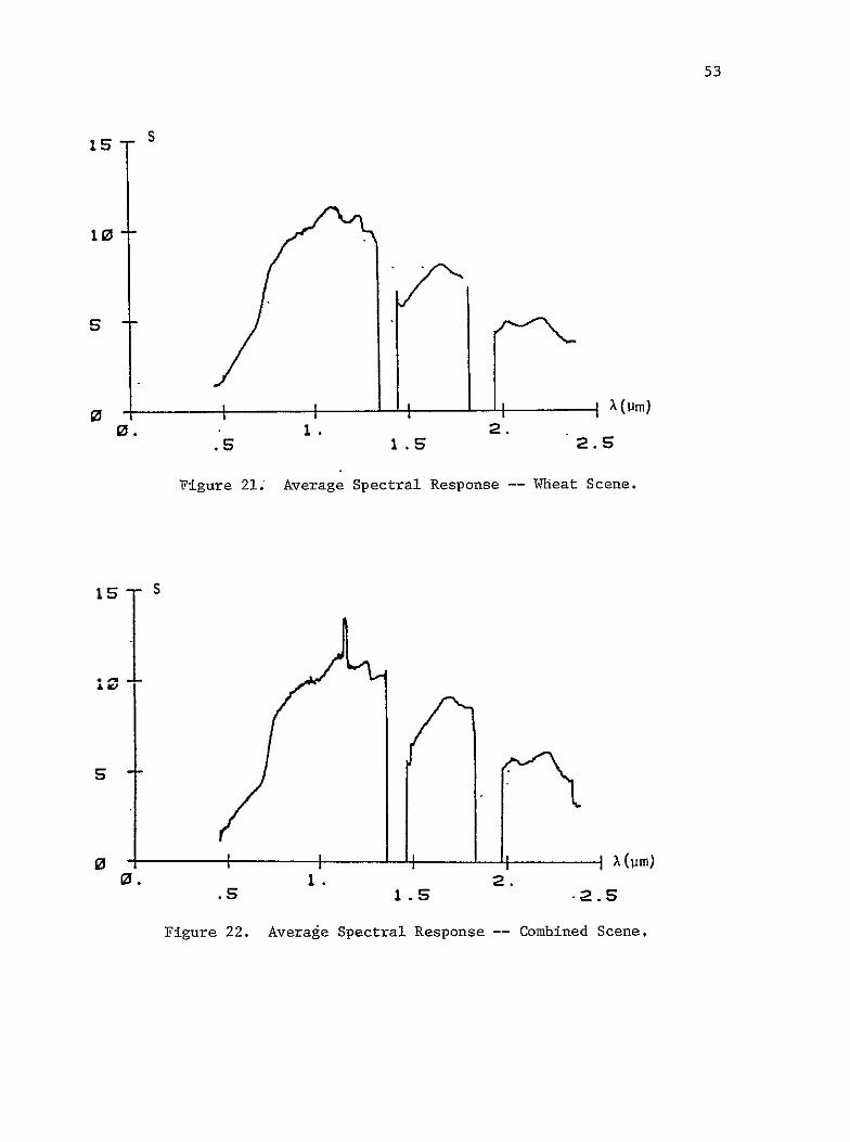
zspectral response provides a relatively good data set for demonstration
-purposes Figures2l and 22 show the average response for both cover
types
In order that the study be carried out in a context that is relashy
tively realistic for multispectral scanners the spectral response -of
the two data sets is divided into a cnumber -of spectral banids The division
is fairly arbit-rary but each band must contain a sufficient number of
data points to ensure accurate parameter estimation for model identifishy
cation The spectrum is divided into 9 bands from 045 pm to 238 pm
with two gaps in the 134-145 pm and 182-196 -pm range -due to atmosshy
pheric absorption see Tables 5 and 6
Table 5 Spectral Bands for Wheat Scene
Band Number Spectral Wavelength Interval (Pm)
1 045-054
2 054-062
3 062-071
4 071-085
5 085-099
6 099-013
7 113-134
8 145-182
9 196-238
Table 6 Spectral Bands for Combined Scene
Band Number Spectral -Wavelength Interval (pm)
1 045-054
2 054-062
3 062-071
4 071-085
5 -085-098
6 098-112
7 112-130
8 145-18 2
9 196-238
53
s15
10-
S
AX(Uir)0 0 1 2 2S
Figure 21 Average Spectral Response -- Wheat Scene
1I X im)
S
0
0 1 5 FS Rsp2s
Figure 22 Average Spectral Response -- Combined Scene
54
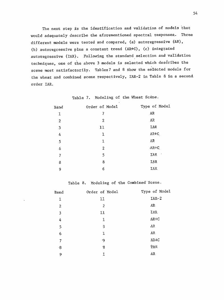
The next step is the identification and validation of models that
would adequately describe the aforementioned spectral responses Three
different models were tested and compared (a) autoregressive (AR)
(b) autoregressive plus a constant trend (AR+C) (c) integrated
autoregressive (I-AR) Following the standard selection and validation
techniques one of the above 3models is selected which describes the
scene most satisfactorily Tables7 and 8 show the selected models for
the wheat and combined scene respectively IAR-2 in Table 8 in a second
order IAR
Table 7 Modeling of the Wheat Sc~ne
Band Order of Model
1 7
2 2
3 11
4 1
5 1
6 2
7 5
8 8
9 6
Type of Model
AR
AR
IAR
AR+C
AR
AR+C
IAR
IAR
IAR
Table 8 Modeling of the Combined-Scene
and Order of Model Type of Model
1 11 IAR-2
2 2 AR
3 11 IAR
4 1 AR+C
5 3 AR
6 1 AR
7 9 AR+C
8 8 tAR
9 1 AR
55
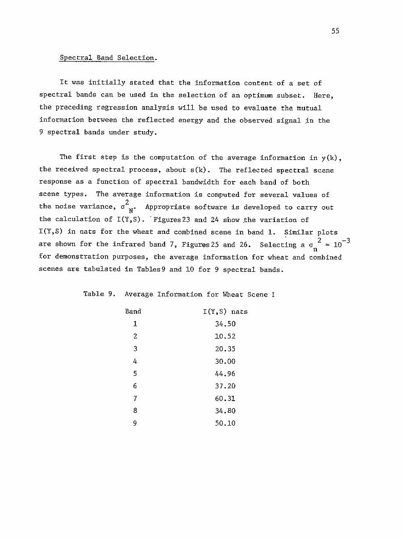
Spectral Band Selection
It was initially stated that the information content of a set of
spectral bands can be used in the selection of an optimum subset Here
the preceding regression analysis will be used to evaluate the mutual
information between the reflected energy and the observed signal in the
9 spectral bands under study
The first step is the computation of the average information in y(k)
the received spectral process about s(k) The reflected spectral scene
response as a function of spectral bandwidth for each band of both
scene types The average information is computed for several values of 2
the noise variance a N Appropriate software is developed to carry out
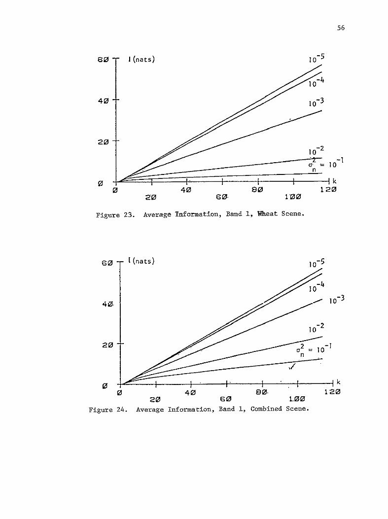
the calculation of I(YS) Figures23 and 24 show the variation of
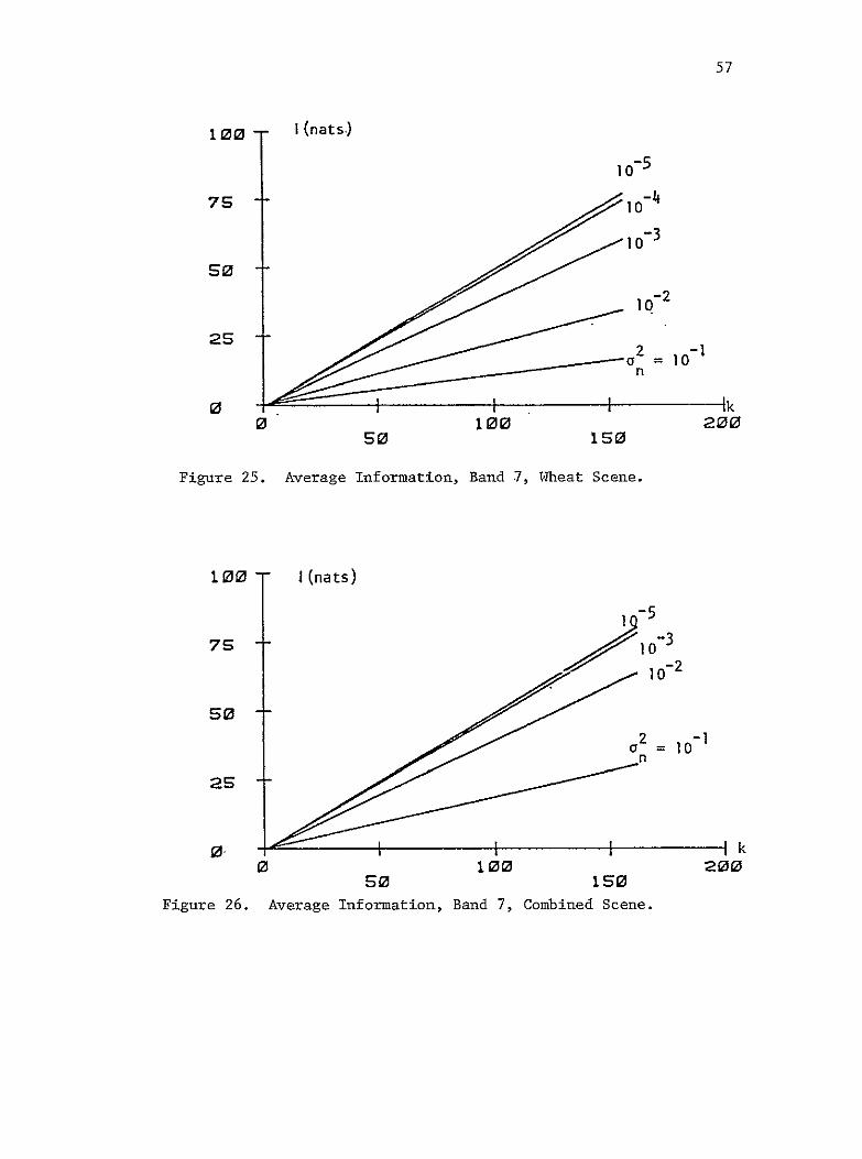
I(YS) in nats for the wheat and combined scene in band 1 Similar plots 2 -3are shown for the infrared band 7 Figures 25 and 26 Selecting a a = 10
for demonstration purposes the average information for wheat and combined
scenes are tabulated in Tables9 and 10 for 9 spectral bands
Table 9 Average Information for Wheat Scene I
Band I(YS) nats
1 3450
2 1052
3 2035
4 3000
5 4496
6 3720
7 6031
8 3480
9 5010
56
0
-51080 I(nats)
40--1shy
20shy
a -Io
k 1
1080400
Figure 23 Average Information Band 1 Wheat Scene
s I(nats) 10-5
10
0 40 0 120
20 40 L00
Figure 24 Average Information Band 1 Combined Scene
57
10 - I (nats)
10-5
7510
so
2s 10shy2
o = i0-1 26
n
0 - k 0 100 200
so ISO
Figure 25 Average Information Band 7 Wheat Scene
100 1(nats)
7S 7-5 10 3
0-2
100 200 s0 IS0
Figure 26 Average Information Band 7 Combined Scene
0
58
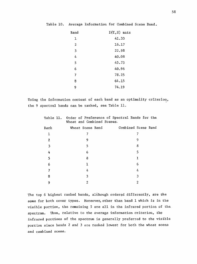
Table 10 Average Information for Combined Scene Band
Band I(YS) nats
1 4133
2 1617
3 2298
4 4008
5 4573
6 4096
7 7825
8 6415
9 7419
Using the information content of each band as an optimality criterion
the 9 spectral bands can be ranked see Table 11
Table 11 Order of Preference of Spectral Bands for the
Wheat and Combined Scenes
Rank Wheat Scene Band Combined Scene Band
1 7 7
2 9 9
3 5 8
4 6 5
5 8 1
6 1 6
7 4 4
8 3 3
9 2 2
The top 6 highest ranked bands although ordered differently are the
same for both cover types Moreover other than band 1 which is in the
visible portion the remaining 5 are all in the infrared portion of the
spectrum Thus relative to the average information criterion the
infrared portions of the spectrum is generally preferred to the visible
portion since bands 2 and 3 are ranked lowest for both the wheat scene
and combined scene
59
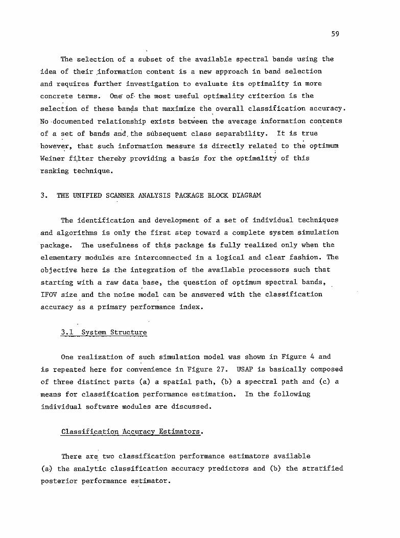
The selection of a subset of the available spectral bands using the
idea of their information content is a new approach in band selection
and requires further investigation to evaluate its optimality in more
concrete terms One of- the most useful optimality criterion is the
selection of these bands that maximize the overall classification accuracy
No -documented relationship exists between the average information contents
of a set of bands and the subsequent class separability It is true
however that such information measure is directly related to the optimum
Weiner filter thereby providing a basis for the optimality of this
ranking technique
3 THE UNIFIED SCANNER ANALYSIS PACKAGE BLOCK DIAGRAM
The identification and development of a set of individual techniques
and algorithms is only the first step toward a complete system simulation
package The usefulness of this package is fully realized only when the
elementary modules are interconnected in a logical and clear fashion The
objective here is the integration of the available processors such that
starting with a raw data base the question of optimum spectral bands
IFOV size and the noise model can be answered with the classification
accuracy as a primary performance index
31 System Structure
One realization of such simulation model was shown in Figure 4 and
is repeated here for convenience in Figure 27 USAP is basically composed
of three distinct parts (a) a spatial path (b) a spectral path and (c) a
means for classification performance estimation In the following
individual software modules are discussed
Classification Accuracy Estimators
There are two classification performance estimators available
(a) the analytic classification accuracy predictors and (b) the stratified
posterior performance estimator
Figure 27 The Block Diagram of the Unified Scanner Analysis Package (USAP)
MS mage
Data
LARSYSData I
RetrievallliteJ
CORELATSpatial - Spatial
Correlationl StatisticsAnalyzer Model
SCANSTAT[Spectral
Saitc Saitc
os
ACAP
Spectral Statistics
Analytic Classification Accuracy Predictor
SPEST
A Pc
Stratified Posterior
Performance Estimator
A Pc
EXOSYS SPOPT SPTES
r
ra
Data Retrieval
SpectralandBand Construction
Spectral Data Ensemble Sample
OptiMum Spectral
Function Calculation
Opt Spect Functions
)0
Data Transformation and
Statistics Calculat[tYV
Band-- --
Specification
Implies path for spectralspatial statistics
Implies path for data or spectral functions
61
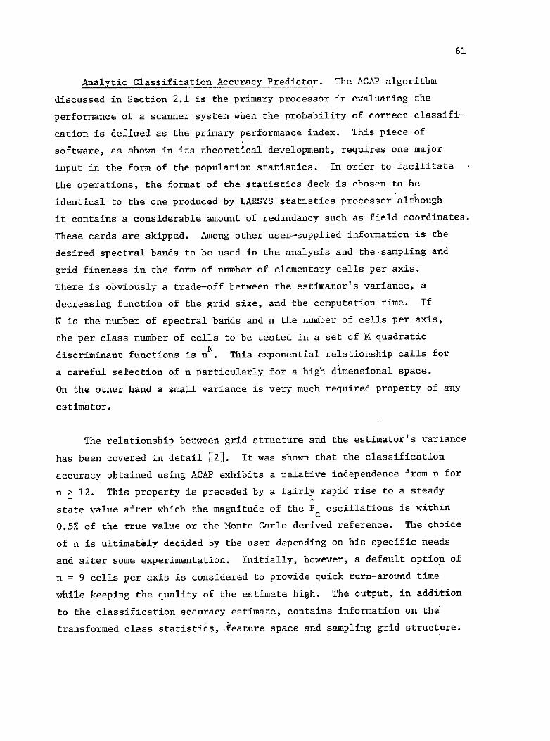
Analytic Classification Accuracy Predictor The ACAP algorithm
discussed in Section 21 is the primary processor in evaluating the
performance of a scanner system when the probability of correct classifishy
cation is defined as the primary performance index This piece of
software as shown in its theoretical development requires one major
input in the form of the population statistics In order to facilitate
the operations the format of the statistics deck is chosen to be
identical to the one produced by LARSYS statistics processor although
it contains a considerable amount of redundancy such as field coordinates
These cards are skipped Among other user-supplied information is the
desired spectral bands to be used in the analysis and the-sampling and
grid fineness in the form of number of elementary cells per axis
There is obviously a trade-off between the estimators variance a
decreasing function of the grid size and the computation time If
N is the number of spectral bands and n the number of cells per axis
the per class number of cells to be tested in a set of M quadratic
discriminant functions is nN This exponential relationship calls for
a careful selection of n particularly for a high dimensional space
On the other hand a small variance is very much required property of any
estimator
The relationship between grid structure and the estimators variance
has been covered in detail [2] It was shown that the classification
accuracy obtained using ACAP exhibits a relative independence from n for
n gt 12 This property is preceded by a fairly rapid rise to a steady
state value after which the magnitude of the Pc oscillations is within
05 of the true value or the Monte Carlo derived reference The choice
of n is ultimatamply decided by the user depending on his specific needs
and after some experimentation Initially however a default option of
n = 9 cells per axis is considered to provide quick turn-around time
while keeping the quality of the estimate high The output in addition
to the classification accuracy estimate contains information on the
transformed class statistiamps feature space and sampling grid structure
62
Stratified Posterior Classification Performance Estimator This
is the software implementation of thealgotthm discussed in Section 22
The maximum conditional aposteriori classprobability is the criterion
for classifitation and error estimation purposes The program does
not provide any options and the size of the internally generated random
data is fixed ACAP and SPEST produce differentbut very close results
Spatial Path
Data Base The input data to the spatial scanner model is via the
multispectral image storage tape containing satellite or aircraft
collected data This tape has been reformatted and is compatible with
any LARSYS processor
Data Retrieval The individual software units can access the
available data base through various system support routines or any of
the LARSYS processors
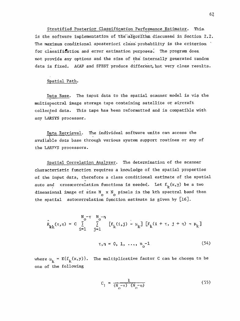
Spatial Correlation Analyzer The determination of the scanner
characteristic function requires a knowledge of the spatial properties
of the input data therefore a class conditional estimate of the spatial
auto and crosscorrelation functions is needed Let f (xy) be a twok
dimensional image of size N x N pixels in the kth spectral band then0 0
the spatial autocorrelation function estimate is given by [16]
No-t No-n
^Rkk(Tn) = C Y Y fk(ij) - k] [fk(i + T j + n) -Vk]i=l j=l
TT1 = 0 1 n -1 (54)
where-pk = Efk(xy)l The multiplicative factor C can be chosen ta be
one of the following
1 (55)CI= (N -T)(N -ii) (
U1(
63
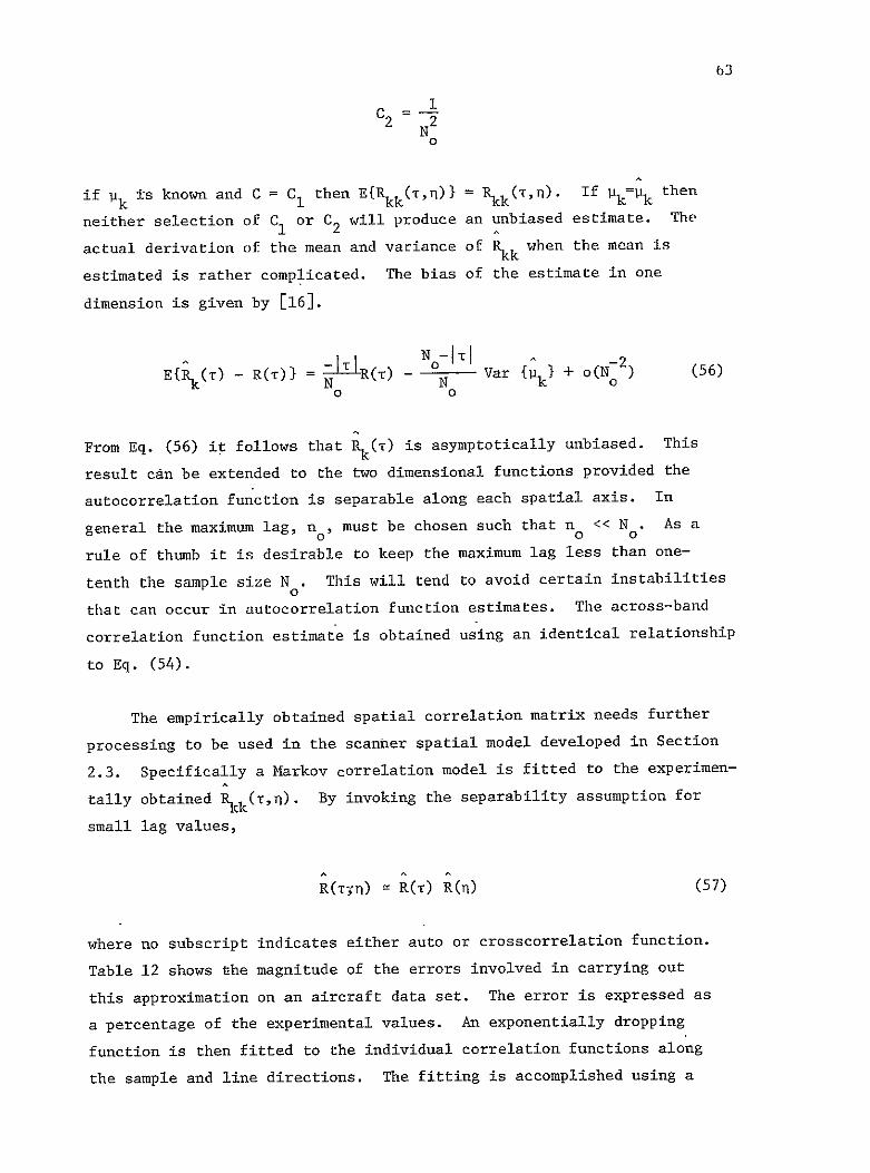
1 C2 =2
if k ts known and C = C1 then ERkk(Tn) = Rkk(Tfn)- If Pk--Ik then
neither selection of C1 or C2 will produce an unbiased estimate The
actual derivation of the mean and variance of Rkk when the mean is
estimated is rather complicated The bias of the estimate in one
dimension is given by [161
N-ITIVar -2 (56)
ERk(T) - R(r) = -R() k + O(No)NN k 0
0 0
From Eq (56) it follows that R( ) is asymptotically unbiased This1
result can be extended to the two dimensional functions provided the
autocorrelation function is separable along each spatial axis In
general the maximum lag n must be chosen such that n ltlt N As a
rule of thumb it is desirable to keep the maximum lag less than one-
This will tend to avoid certain instabilitiestenth the sample size N 0
that can occur in autocorrelation function estimates The across-band
correlation function estimate is obtained using an identical relationship
to Eq (54)
The empirically obtained spatial correlation matrix needs further
processing to be used in the scanner spatial model developed in Section
the experimenshy23 Specifically a Markov correlation model is fitted to
tally obtained lkk(Tr) By invoking the separability assumption for
small lag values
R(rn) R(r) R(n) (57)
where no subscript indicates either auto or crosscorrelation function
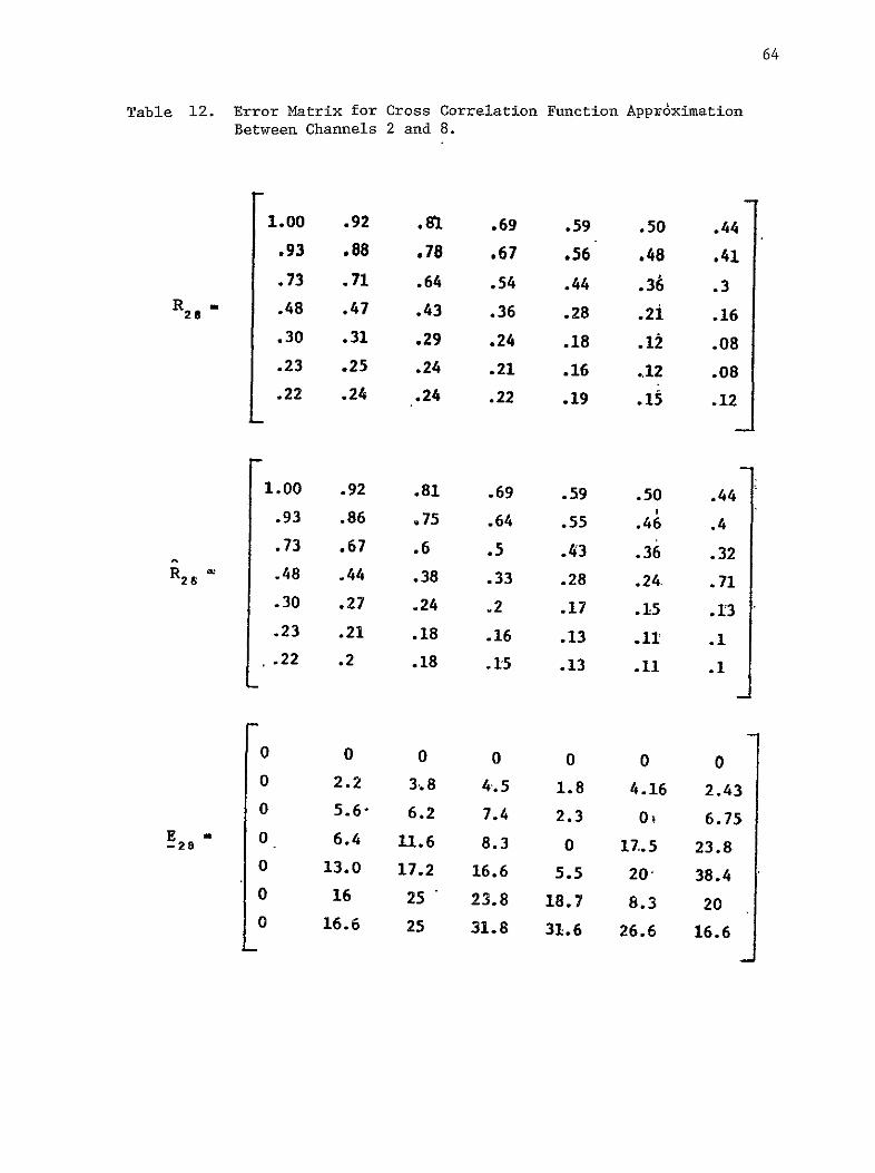
Table 12 shows the magnitude of the errors involved in carrying out
this approximation on an aircraft data set The error is expressed as
a percentage of the experimental values An exponentially dropping
function is then fitted to the individual correlation functions along
the sample and line directions The fitting is accomplished using a
64
Table 12 Error Matrix for Cross Correlation Function Appr6ximation Between Channels 2 and 8
100 92 81 69 59 50 44 93 88 78 67 56 48 41
73 71 64 54 44 36 3 R28 48 47 43 36 28 2i 16
30 31 29 24 18 12 08
23 25 24 21 16 12 08
22 24 24 22 19 15 12
100 92 81 69 59 50 44 93 86 75 64 55 46 4
73 67 6 5 43 36 32 R28 48 44 38 33 28 24 71
30 27 24 2 17 15 13
23 21 18 16 13 11 1 22 2 18 15 13 11 1
0 0 0 0 0 0 0 0 22 38 45 18 416 243 0 56- 62 74 23 O 675
28E 0 64 116 83 0 175 238 0 130 172 166 55 20 384
0 16 25 238 187 83 20 0 166 25 318 316 266 166
65
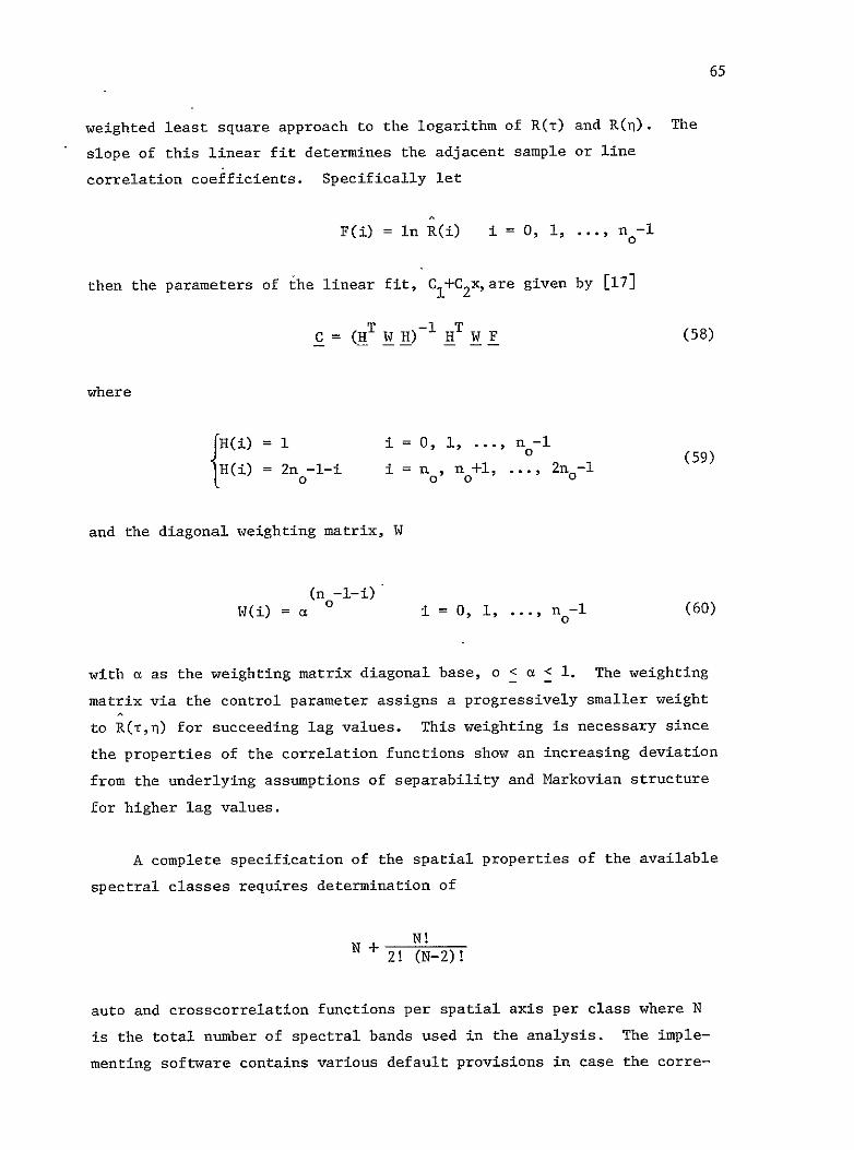
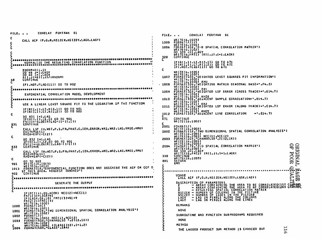
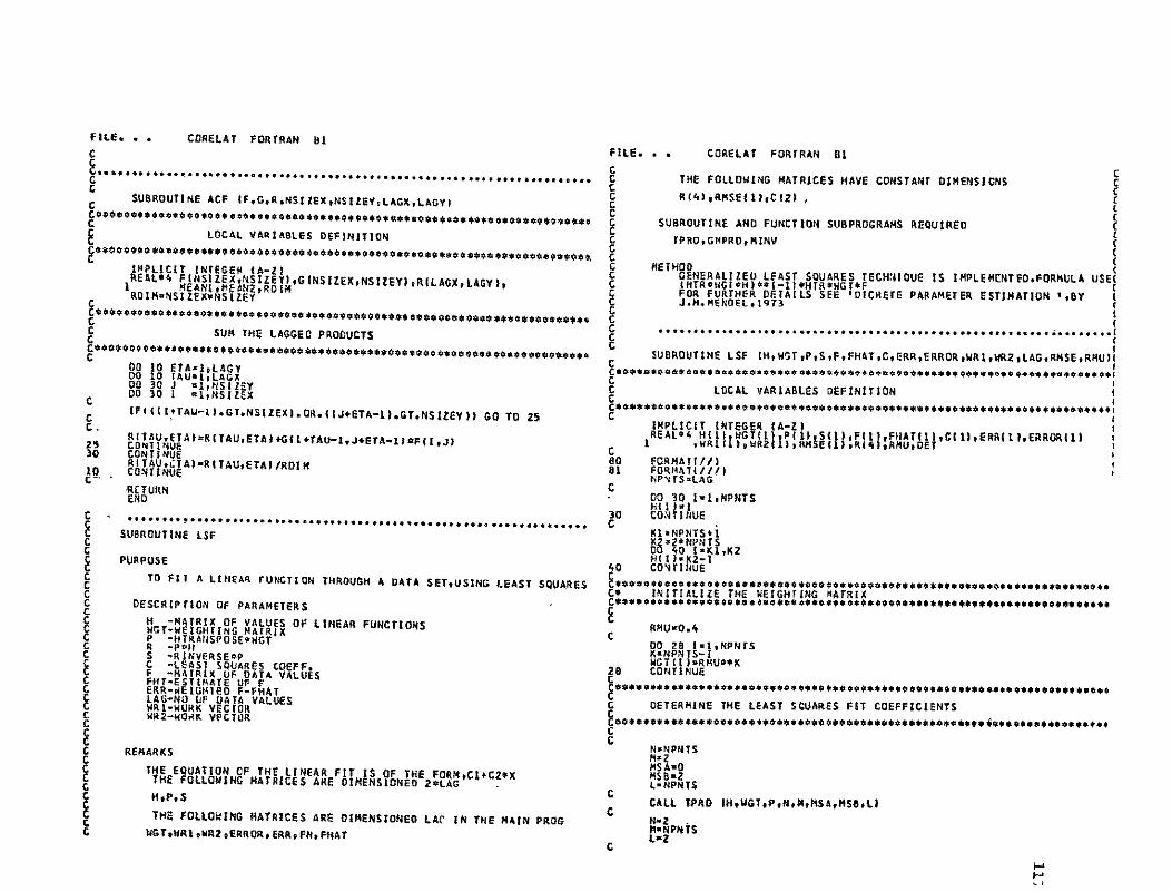
weighted least square approach to the logarithm of R(T) and R(n) The
slope of this linear fit determines the adjacent sample or line
correlation coefficients Specifically let
F(i) = ln R(i) i =0 1 n -l
0
then the parameters of the linear fit CI+C 2xare given by [17]
C = (HT W H) -I HT W F (58)
where
E(i) = 1 = 0 no(59)0
0 i no+lH(i) 2n -l-i = 0o 0O 2n -i
and the diagonal weighting matrix W
(n -1-i) i = 0 1 n - (60)W(i) = a
with a as the weighting matrix diagonal base o lt a lt 1 The weighting
matrix via the control parameter assigns a progressively smaller weight
to R(Tn) for succeeding lag values This weighting is necessary since
the properties of the correlation functions show an increasing deviation
from the underlying assumptions of separability and Markovian structure
for higher lag values
A complete specification of the spatial properties of the available
spectral classes requires determination of
N N + 2 (N-2)
auto and crosscorrelation functions per spatial axis per class where N
is the total number of spectral bands used in the analysis The impleshy
menting software contains various default provisions in case the correshy
66
lation properties of the input data differs considerably from the aforeshy
mentioned assumptions
The user specifies the area to be correlated by a run table entry
run number followampd by the field coordinates In order to perform either
the auto or crosscorrelation operations appropriate spectral bands(s)
need to be specified The maximum lag no in computing R(tn) is also
a variable and is entered as a percentage of the image size in pixels
The value of n is dependent on the size of the area to be correlated 0 ^
Since the magnitude of R(Tn) for Landsat data is generally negligible
for more than 4 or 5 pixels lag n as a percentage can take on small
values for large fields and vice versa
Scanner IFOV Model The scanner IFOV software is the computer
implementation of the scanner characteristic function discussed in
Section 23 The input consists of (a) spectral covariance matrix
(b) spatial correlation matrix along the samples (c) spatial correlation
matrix along the lines and (d) IFOV size in terms of the number of high
resolution pixels A standard LARSYS statistics deck produced by the
statistics processor constitutes the first item The spatial correlashy
tion information in entered through an N x N symmetric matrix the (ij)
element of which
-a Pj = e ij
a is estimated
by the spatial correlation software The IFOV size is expressed on a
relative scale in terms of the number of high resolution pixels within
1 IFOV of the scanner PSF eg 1 2 3 etc There are two choices
available for the functional form of the PSF Gaussian and rectangular
is the pixel-to-pixel correlation for bands i and j 11
The output generated by this software module is a spectral statistics
deck which is the input class statistics transformed by the scanner
characteristic function This deck is used as input to the ACAP processor
67
Additive Noise Model By virtue of the parametric approach adopted
here the incorporation of the noise effect takes on a simple form The
noise statistics is characterized by a zero mean vector and a diagonal
covariance matrix with zero off diagonal elements This matrix is then
simply added to each class covariance matrix
2 nI
2 Gn
2
+ (62)
f f
2 a nN
The diagonal elements of G2 determines the SNR in each spectral -N i
band By the appropriate selection of a s different SNR can be
specified for each band Let a denotenhe variance of the noise-free
signal at the scanneroutput then the SNR in the kth spectral band is
defined by
(SNR)k = af2 n (63)
The choice of equal oic unequal SNR in different bands based on experimental
or theoretical results is at the analysts discretion
Spectral Path
Data Base and Retrieval EXOSYS is a software package which provides
access to field measurement data taken with a variety of field instruments
A brief overview of the EXOSYS package will be given here with more detail
available in the EXOSYS manual [18] Data is collected and stored on
magnetic tape in field measurements format During the reformatting
procedure the data is calibrated and ancillary information such as
68
weather readings soil conditions and plant growth status is placed in
the identification record for each run
There are three processors in EXOSYS which are used to access the
field data information - IDLIST GSPEG and DSEL The IDLISW processor
scans the tape and lists information from the identification record as
required One can use this information to select appropriate runs-to
represent informational classes
The GSPEC processor provides a punched deck consisting of the
numerical values of the spectral response function for all of the desired
runs One can select a set of run numbers as input and the output will
consist of a punched deck Options exist for plotting the spectral
response functions for the desired runs
The DSEL processor simulates rectangular spectral channels and
uses data from the tape to evaluate the response in each channel for
the ensemble The inputs are the spectral band locations and the run
numbers on the data tape The output is a set of statistics for the
specified channels
Optimum Spectral Basis Function System For the optimum spectral
function calculation the output of the GSEC processor is required The
appropriate ensemble can be selected by specifying a set of identificashy
tion parameters such as date of collection scene type run number etc
The cards containing the numerical values for the spectral response
functions are used and stored on- disk in a format which is compact and
convenient for future processing by the program SPRDCT The files that
are stored on disk may be transferred to magnetic tape for future use to
avoid repeating the procedure involving the EXOSYS package SPRDCT
requires some information to be entered at the terminal to provide ID
information for the ensemble A list of all runs used by run number is
printed after the data has been stored on disk
69
Optimum Basis Function Calculation The calculation of the optimum
set of basis functions for an ensemble is accomplished by solving the
matrix equation
4r = KWF (64)
to get the eigenvalues ll O2 aN and the eigenvectors h 2 N
N1The matrix 0 is the matrix of eigenvectors 0 = [1i 2 and F is
the diagonal matrix of eigenvalues
0a1
a2 (65)
aN
The matrix W is a diagonal matrix of weights
Wl 0
W 2 (66)
WN-
R is the covariance matrix for the ensemble Let the mean vector for the
ensemble be m = [mI m2 mNT then
R = E (x-m) (xj-m)T (67)
The maximum likelihood estimate is
N
1 = kN T
ki Ns I ~ (Xik-m) (x kk-m )68
7Qt
where N is the number of sample functions in the ensemble
If we let A=KW then A is a real general matrix An algorithm for
solving for tha eigenvalues-and eigenvectors of a real general matrix is
available [19] and is used here with only slight modification The
algorithm makes use of Householders method and the QR double-step iterashy
tive process to compute the eigenvalues The eigenvectors are obtained
by the inverse iteration technique A sorting routine-was added to order
the eigenvalues and the corresponding eigenvectors
The required inputs are the data in the appropriate format and the
weight function The output of this processor is a set of N eigenvectors
or baslis functions punched onto cards Also the eigenvalues and means=
square representation error are printed The eigenvectors canbeplotted
using GCS subroutines
Data Transformation and Statistics Calculation The ejgenvectors
are used to perform a linear transformation on the original data vectors
[X The transformed vectors MY have the desired properties provided
by the Karhunen-Loive expansion Each element of the transformed-vector
is given by
Yi = ilxl + i2x2 + + 4iNXn (69)
where ij is the jth element of the ith eigenvector
The inputs to this processor are the eigenvectors and the data set
stored on the disk The output is the set of statistics for each class
The statistics are printed and punched on a deck of cards for future
processing
4 USERS GUIDE TO USAP
The block diagram of the scanner parameter study Figure 27 is made
operational by a collection of compatible software packages Each module
is individually compatible with the LARSYS environment facilitating
71
incorporation of LARSYS processor in the overall system performance
evaluation This section provides a guide for the acquisition and
execution of each program available on the LARS IBM 370148 computer
system
Prior to a discussion of the individual modules some general remarks
are inorder The access to this program library is simplified by the
allocation of two special disk storage devices designated by DHSYS and
DHDSK The former contains the text version of the software while the
latter holds the source These devices can be accessed using the
appropriate GETDISK commands
GETDISK DHSYS
and
GETDISH DHDSK
these commands will establish the proper links in a Read-Only mode and
USAP initialization is complete In the following subsections the
required input and necessary steps to run each program are discussed
41 The Classification Accuracy Estimators
There are two parametric classification accuracy estimators
available to the USAP user (a) the analytic classification accuracy
predictor (ACAP) and (b) the stratified posterior classification
accuracy estimator (SPEST) The theoretical aspects of these processors
have been discussed in Section 2 Here is a guide to their software
implementation
Analytic Classification Accuracy Predictor
This program evaluates the performance of a Bayes classifier when
the populations statistics are multivariate normal The following
control cards are required
72
ontrol Word -Description
ACAP This card specifies the particular processor
requested
CHANNELS The desired subset of the available channels is given here Note that the numbers appearing on this card are the order of the selected channels not theiractual number For example if the available channels are 8 9 12 14 and channels 8 9 and 14 are requested CHANNEL card should read 1 2 4
CLASSES This card specifies the name of each class Each name must be placed in a field 7 characshyters long followed by a blank The continuashy-tion card if required must have the word CLASSES at the beginning
GRID This quantity controls the quality of the estimate The higher the number the closer the estimate is to the true Bayes error rate (See ampstimated CPU timefor more details)
END This card signals the end of the control card Stat deck follows immediately
Remarks The ACAP processor in its current form is capable of
handling up to 20-classes and 8 spectral bands The extensions of
these parameters presents no conceptual difficulty The required statisshy
tics deck is a standard LARSYS produced deck with no modifications It
must be punched in the character format however
How to Run the Program Make sure the DHSYS disk has been accessed
properly One reader file consisting of the control cards followed by a
statistics deck is required Type ACAP in the CMS environment Approshy
priate terminal and printer output is produced
Example of control card set up
ACAP CHANNELS 134 CLASSES SOYBEAN ALFALFA WHEAT END
Since GRID card is not included its default value (9) is selected
73
Estimated CPU Time The execution time is quite sensitive to the
GRID card specifying the number of cells per axis For the default
grid size and a 4-dimensional space it takes approximately 2 minutes of
CPU time per class to provide the requested classification accuracy
estimates The CPU time is most sensitive to the dimensionality of the
feature space Hence if the number of spectral bands is limited (less
than 4) considerable increase in GRID number is possible The default
number of cells per axis is considered to be the minimum while still
providing acceptable performance Increasing the parameter improves
the quality of the estimate somewhat at the expense of higher CPU time
The choice is left at the users discretion
Stratified Posterior Error Estimator
This program is identical in purpose but different in approach to
the ACAP processor GivEna set of multivariate normal populations
SPEST provides the classification accuracies associated with each class
using an internally generated random data base The different estimation
procedures between the two methods is transparent to the user
Description of the Control Cards
Control Word Description
SPEST This card specifies the particular processor
requested
CHANNELS The desired subset of the available channels
is given-here Note that the numbers appearing
on this card are the order of the selected
channels not their actual number
CLASSES This card specifies the name of each class Each name must be placed in a field 7 characshyters long followed by a blank The continuashytion card if required must have the control
word CLASSES in the beginning followed by
the rest of the names
END End of the control cards
74
Remarks In usage this program is identical to ACAP The
standardLARSYS statistics deck follows the control and disk immediately
Printer output contains the estimated conditional classification
accuracies By virtue of their separateapproaches ACAP andSPEST
provide different but very close estimates of the correct 5classification
accuracies
How to Run the Program The reader file contains the control cards
followed by the LARSYS statistics deck A sample control card deck
follows
SPEST
CHANNELS 124
CLASSES ALFALFA SOYBEAN WHEAT END
42 Spatial Path
The spatial path in USAP consists of two main software units The
spatial correlation analyzer CORELAT and the SCANNER IFOV model
SCANSTAT
Spatial Correlation Modeling This program is a2-dimensional
spatial correlator the primary output of which Is a normalized spatial
auto (cross) correlation matrix for any specifieamp area The user specishy
fies the coordinates of the desired segment in the formof am injtial and
final line and column along with the appropriate spectral bands (s)
Following the estimation of the correlation matrix the expQnential fit
option if invoked will fit an exponentially dropping function to- the
experimental values of R k(t) or k-n) using a wetghtedi linear least squares technique
75
Description of the Control Cards
Control Word Control Parameter Description
CORRELATE This card specifies the particular
processor requested
INPUT RUN() Run number of the desired area TAPE() Tape number of the desired area FILE() File number of the desired area
BLOCK LINE() Initial and final lines COLUMN() Initial and final columns
FUNCTION AUTO Autocorrelation function requested CROSS Crosscorrelation function requested
CHANNELS Channels used for correlation operation
SAMPLELAGt Maximum cross track lag used as a percentage of the total number of samples
LINELAGt Same as SAMPLELAG except for along track lag
EXPOFITt If included exponential fitting operation is carried out
END End of control cards
Remarks This program is capable of processing areas containing
up to 2400 pixels The maximum lag default is set at 20 percent of
the total number of lines and columns Both quantities can be altered
by user supplied control cards The exponential fit option provides a
pixel-to-pixel correlation coefficient for the channel(s) specified
This number is computed from the estimated parameters of the exponential
correlation model
How to Run the Program The only required reader file is the
control card deckan example of which follows
t optional
76
CORRELATE INPUT RUN (74028500) TAPE (2689) FILE (3) BLOCK LINE (125) COLUMN (125) FUNCTION AUTO CHANNELS 2 SAMPLELAGt 25 LINELAGt 25 EXPOFITplusmn
END
after DHSYS disk has been properly linked to type CORELAT tp start
execution Appropriate terminal and printer output isgenerated
Scanner IFOV Model
This program computes the spectral statistics of a population at
the output of a multispectral scanner provided the data spatial correlashy
tion approximately follows a Markov model The scanner IFOV shape is
limited to either a Gaussian or rectangular shape No assumptions
are made or indeed required about the type of the population statistical
distribution
Description of the Control Cards
Control Word Description
SCANSTAT This card specifies the particular processor
requested
CHANNELS The desired subset of the available channels
is given here Note that the numbers appearing
on this card are the order of the selected channels not their actual number
CLASSES This card specifies the name of each class Each name must be placed in~a field 7 characters long foliqwed by a blank The continuation card if required must have the control work CLASSES in the beginning
followed by the rest of the names
IFOV This card specifies theJIFOV size of the
scanner in terms ofhigh resolution input pixels
t optional
77
APERTURE The choices here are GAUSSIAN or RECTANGULAR
SNRi Output signal energy to noise energy in dB
PUNCHplusmn The output statistics is punched out in an
ACAPSPEST format Redundancies are added to replace field description cards
END End of control-cards
Remarks This program is limited to 20 classes and 8 specfral
bands Execution time is quite short and extension of those parameters
is straightforward The input data immediately following the control
cards consists of 3 parts
1 Standard LARSYS statisticsdeck in character format
2 Spatial correlation parameters (cross track) are entered via a
NXN symmetric matrix where N is the number of channels The
(ij) element of this matrix is the adjacent sample correlation
between channels i and J The lower triangular part of this
matrix is punched in a 5 (EI37lX) format
3 Spatial correlation parameter matrix except for along track
pixels
The above decks follow the control cards in the order listed The
signal-to-noise ratio is defined as the ratio of the output signal
energy in a particularchannel (diagonal element of the class covariance
matrix) to the noise energy in the same bands expressed in dB and defined
by
10 log1 0 a k2(SNR)k =
k 10 sk nk
where k refers to the particular spectral band
t optional
78
How to Run the Program Onereader file consistingof 4 consecutive
decks and appropriate link to DHSYS disk is required before the program
execution An example of a control card set up follows
SCANSTAT
CHANNELS 124 CLASSES ALFALFA SOYBEAN WHEAT IFOV 2 APERTURE GAUSSIAN SNRI 10 PUNCHI ENDt
The output consists of an ACAPSPEST compatible statistics deck for
the modified population This deck can be used in the ACAP-SPEST processors
to obtain the new set of classification accuracy estimates
43 Spectral Path
The spectral path in USAP consists of three main pieces of software
(a) data retrieval through EXOSYS processor (b) optimum spectral function
calculation and (c) data transformation and statistics calculation
Procedure for Computing and Evaluating Optimum Basis Functions
Data Retrieval The data retrieval system is stored on EXOSYSDV and
it is necessary to define storage as 768K A card file containing the
data points for each run will be constructed on a temporary disk
(25 cylinders) It is desirable to make the temporary disk a P-disk
and the permanent user disk a T-disk
In CMS
RELEASE 191 P LOGIN 191 T GETDISK TEMP MODE P25CYL NO-UFD
plusmnnntn1l
79
In CP
I EXOSYSDV CCINPUT TERMINAL RUN EXOSYSDV
The control cards will be entered through the terminal The tape on
which the data is stored must be specified as well as the cover type
and the collection date A typical sequence of cards is as follows
$ TAPE 4896 $ GSPEC
GRAPH SPEC (SPRING WHEAT) DACO (770508) LIST NO LIST
OPTIONS PUNCH NOGRAPH END
$ END $ EXIT
The runs taken over Williams Co North Dakota for May 8 1977 are on
tape 4896 The crop species is spring wheat and the collection date is
May 8 1977 The output is a deck of cards with one hundred data values
for each run punched onto the cards Header information must be flushed
at the line printer Return the system to CMS and read the cards onto
a disk file SPR100 DATA The number of records in the file is equal to
the number of runs This number should be recorded as it will be needed
later This procedure is repeated for the second class The cards from
GSPEC are read onto the file INPUT DATA and the number of records
recorded The two files are combined by typing (in CMS)
COMBINE SPR100 DATA P1 SPR 100 DATA P1 INPUT DATA P1 ERASE INPUT DATA
This procedure is repeated until all classes have been included in the
file SPR 100 DATA The crop species SUMMER FALLOW and PASTURE are used
in GRAPH SPEC() to complete the data set
At this point the program SPRDCT is loaded and rum A disk file
will be created using DSRN of 2 and file type FUNC The following
information is requested at the terminal by SPRDCT
Experiment Number 100
Number of Classes 3
Number of Sample Points per Run 100
(Dimensions)
Class Name Wheat Fallow Pasture
Number of Samples per Class 664 437 16-
The information is requested and is entere-dbetwpen the slash
marks right justified
At this point the data is ready to be used by the system It is a
good iaea to store the file on tape for future use Type
TAPMOUNT 156 TAP2 RI T DUMP SPR 100 FUNC Pl
The tape on which the data is stored is 156 in this example To recall
the data to the disk type
TAPMOUNT 156 TAP2 RO (If not already mounted) T SLOAD SPR 100 FUNC
Note that the 2-disk -must be a large -fairly empty -disk (10 cyl)
The format for data storage is
81
ID
Run 1
100 DataVaeClass 1 Values
Run 2
100 Data Values
Class 2
ID Information Record
Item
Date
Exp Number
Number of Classes
Number of Dimensions
Number of Samples for Class 1
Number 6f Samples for Class 2
Number of Samples for Class 3
Number of Samples for Class 4
Number of Samples for Class 5
Number of Samples for Class 6
Number of Samples for Class7
Name of Class 1
Name of Class 2
Name of Class 3
Name of Class 4
NnMr nf CAn~ 9
Words
1-15
16
17
18
21
22
23
24
25
26
27
30-39
40-49
50-59
60-69
70-79
mL4
Name of Class 6 80-89
Name of Class 7 90-99
Optimum Spectral Functions Calculations
Once the data set is on disk it is necessary to issue the following
CMS commands to compute the eigenvectors
FILEDEF 2 DSK-P4 SPRIOO FUNC RECFM VS LRECL 400 BLKSEZE 400 (PER CP SP PUN TO USERID LOAD SPOPTM (XEQ
44 Example Outputs
This section presents a sample output for the individual software
units used in USAP The example set consists of sample outputs from the
ACAP and SPEST processors CORELAT and SCANSTAT in the spatial path and
SPOPT and SPTES in the spectral path Graham Co Kansas is used as the
test site
Classification Accuracy Estimators
The following control card set up is used for the ACAP processor and
output is shown in Table 13
ACAP
CHANNELS 1234 CLASSES BARESOI CORN SOYBEAN WHEAT END
The required control cards for the SPEST processor are
SPEST
CHANNELS 1234 CLASSES BARESOI CORN SOYBEAN WHEAT END
the output is shown in Table 14
Table 13 ACAP Sample Output
ANALYTIC CLASSIFICATION ACCURACY PREDICTION- A C A P
SAMPLING GRID CHARACTERISTICSO
GRID SIZE= 9 CELLS PER DIMENSION
TOTAL NO OF CELLS IN THE GRID 6561
TRANSFORMED FEATURE SPACE CHARACTERISTICSO
EIGENVALUESO
29182E 01 11413E 01 13430E 00
EIGENVECTORSO
2105E-01 20478E-01 82319E-01458446E-01 82659E-01 -15239E-01
-67334E-03 19331E-01 -53271E-0186342E-01 -4872BE-01 -12389E-01
TRANSFORMED MEAN VECTORSO
11654E 01 23928E 01 38200E-01-2Z766E 00 15Z48E 01 13871E-0113111E 01 51333E 00 -59814E-01
00 00
P R O B A B I L I T Y
CLASS WHEAT
76125E-01
-v
48593E-01 -28873E-01 82390E-01 41283E-02
-54T50E-02 10838E-01 10702E 00 00
O F C 0 R R E C T C L A S S I F I C A T I O N 93486 1
TOTAL PROB OF CORRECT CLASSIFICATION= 89287 PERCENT
00
Table 14 SPEST Sample Output
STRATIFIED POSTERIOR ERROR ESTIMATOR
P R 0 B X B II T Y
CLASS BARESQI
0 F C 0R R E C T C L A S S I F I C A T I 0 N = 79218(
P R 0 BA B I I-| T Y
CCASS CORN
0 F C 0 R R E C T C L A S S I F I C AT I 0 N = 92721(
PR0BABIL ITY
CLASS
O F
SOYBEAN
C O R R E C T C L A S S I F XC A TI 1O N = 96359(
P a s A 1 II TLY
CLASS
0 F
WHEAT
C On R E C T C L A S S I F I C A T 1 0 N - 92614(
OVERALL PROBABILITNy1QF CORRECT RECOGNITION= 90220
do
85
Spatial Path
The control card set up for CORELAT is as follows
CORRELAT
INPUT RUN(74028500) TAPE(2689) FILE(3) BLOCK LINE(5098) COLUMN(5098) FUNCTION AUTO CHANNELS 1 EXPOFIT END
The sample output is shown in Table 15
The control card set up for SCANSTAT is as follows
SCANSTAT
CHANNELS 1234 CLASSES BARESOI CORN SOYBEAN WHEAT IFOV 2 APERTURE GAUSSIAN END
The sample output is shown in Table 16
Spectral Path
The optimum basis function calculation and computation of the
transformed data statistics comprises the main spectral processors The
sequence of required commands has been shown in Section 43 The
following example is a weighted basis function calculation
The weighting function w(X) is zero for the water absorption bands
near 14 and 18 micrometer and zero elsewhere on the interval (4-24 pm)
The printer oi-tput is shown in Table 17 listing the first 30 eigenvalues
The first 4 eigenvectors are sent in card format to the reader They
can be stored on the disk by issuing the command
0 READ EIG00 DATA Tl
Table 15 CORRELAT Sample Output
TWO DIMENSIONAL SPATIAL CORRELATION ANALYSIS
CHANNELSO 1 1
2-D SPATIAL CORRELATION MATRIX
100 03 050 036 O28 0123 019 D1f3 008
070 06Q- 044 033 026 020 017 012 007
050 Q45 O36 027 021 017 014 010- 005
038 037 031 024 01-7 013 011 008 003
031 032 027 U21 014 011 010 008 004
025 026 023 06 011 009 007 005 0 02
02 0 020 0 18 013 010 007 O0amp O05 003
014 015 4 0lO 007 005 O94- 004 002
010 0 11t 012 01i 009 040- 0031 002 0001
WEIGOTEDzLEAST- SQUARES FIT INFORMATION-
WEIGHTING MATRIrX DIAGONAL BASE=O40 WEIGHTED LSF ERROR (CROSS TRACK)= 01037569E-02gtADJACENT SAMPLE CORRELATION= 0793716E 0-WE IGHTED LSF ERRORU(ALONG TRACK-) 673b4634Et05-AJDJACENT LINE CORRELATI0N - 7026460E 00
I I
Table 16 SCANSTAT Sample Output
SCANNER
APERTUREO
OUTPUT
GAUSSIAN
STATISTICS
IFOV SIZEO 2 HIGH RESOLUTION PIXELS
CLASS CORN
INPUT COVARIANCE MATRIX
929
1226 1979
1063 1637 1609
443 714 624 345
OUTPUT COVARIANCE MATRIX
486
461 1037
400 615 843
167 268 234 181
00
rt
88
LARQOPATONY FOR APPLICATIONS OF REMOTE SLNSIIGPUPFUE UN4IVEPS1TY SAMPLE FUNCTION I4FOrLATION 10 JULY 1978
100 NUMBER OF CLASSES 3 CLASSWHEAT NUMBER OF SAMPLE FUNCTIONS664 CLASSFALLOA
EXP NO
NUMBER OF SAMPLE FUNCTIONc437 CLASS PASTURE NUMER OF SAMPLE FUNCTIONS 164
WEIGHTING FUNCTION NUIARE 3
N 1 2 3
EIGENVALIJE 3114133 2293520 211702
VAR (GA ) 3070752 1665619
14191
VAR (PHI)00086 0OOb700104
MEAN-SQUARE EPROR 29915674q6V8d4748 46J4554
4 154660 07574 00126 3316b544 5 88838 02499 00106 242047e4 6 7 q
57765 35611 26887
01057 00402 0029
0012 0OLj700573
jt50amp2qi4947187 1f25848 9
23128 00169 00635 4945677 10 1i
18363 14195
00107 00064
0044 00663
o 1033 06u9800
12 19
12304 09300
000i 00027
00043 00336
b4b 4q4452-464
14 06806 00015 00338 38465-28 15 16
05217 03517
00009 00004
00351 Olo 6
J327086 2975436
17 IR
03138 02945
00003 00003
0314 047o2
6o15)923o7111
19 20
02771 02336
00002 00002
03430 0211 6
2090019 18D64 11
21 02102 00001 357eb2 1646236 2 02092 0-0001 357220 1437049 23 24
01792 01514
00001 00001
014-69 oz238
127806 1106359
25 01452 00001 05u6 0961120 2r 01137 00000 00943 uB+458 27 P 2Q
00976 00851 00744
00000 00000 00000
0101 01318011n3
0749854 U664 7 8509tU391
52
30 00583 00000 0c213 05j211-2 q-
Table 17 Eigenvalue and Mean-Square Representation Error for the Data Set
89
A GCS routine was used to plot the graphs of the eigenvectors the
first of which are displayed in Figures 28 through 31
The statistics for the first 4 terms are computed by using the
same FILEDEF command as above plus
CP SP PUN TO USERID 0 PUNCH EIG100 DATA TI LOAD SPTES (XEQ)
The program will ask NUMBER OF TERMSto get all 4 terms type 4
The output will be a statistics deck with the following format
Card
I
2
Number of Classes Number of Terms
Apriori Probabilities for each Class = lNumber of Classes
Mean Class I [Foimat (20A4)]
Covariance Matrix Class 2
Mean Class 2
The covariance are in upper triangular form This statistics deck
can be used as the input to the classification error estimator algorithms
Table 18 is a sample of the statistics obtained from the data set using
the first 4 optimum basis functions Also the statistics were used as
input to the classification performance estimator SPEST to get an
estimate of the probability of correct classification
4
90
-
- 1
19 24-I 9 14 19 24 A A
WRVELENGTHt MICROETERS)WAVELENGTH (MICROMETERS)
Figure 28 Eigenvector 1 Figure 294 Eigenvector 2
91
3(A) 04()
- 2
19 2 9 19 2A
WRVELENGTH (MICROMETERS] WRVELENGTH (MICROMETERS)
Figure 30 Eigenvector 3 Figure 31 Eigenvector 4
92MEAN VECTOR
-20063751 220529 45466 188553
COVARIANCE MATRIX
3125391 -244102 628445
84233 -207412 140594 -52539 -86057 45237 1226-12
MEAN VECTOR
-2021029 352806 57945 163977
COVARIANCE MATRIX
2447227-693594 1525959 -158333 103513 240876 -22070 13667 -07130 123877
MEAN VECTOR
-1875431 548315 82578 190705
COVARIANCE MATRIX
2861719 -12813 1684688
-192971 -477388 290520 103206 543401 -164006 261763
PROBABILITY OF CORRECT CLASSIFICATION FOR CLASS I = 09187
PROBABILITY OF CORRECT CLASSIFICATION FOR CLASS 2 = 06624
PROBABILITY OF CORRECT CLASSIFICATION FOR CLASS 3 = 09003
OVERALL PROBABILITY OF CORRECT RECOGNITION 08270
Table 18 SPTES and SPEST Sample Output Using the First 4 Eigenvectors and Estimates of the Classification Accuracy
93
5 SUMMARY
The task of evaluating the performance of a multispectral scanner
system while incorporating every spatial spectral electronic and teleshy
metric parameter is exceedingly complicated The primary objective of
this project has been the investigation of the two important and most
relevant in remote sensing applications of scanner parameter namely
spatial and spectral The development of analytic techniques for system
performance evaluation differentiates the approach adopted here from
other experimental methods This property provides an ease of parameter
manipulation not available through some heavily data dependent algorithms
Although the development of individual components of such systems is
fundamental to the overall system operation it is the logical and proper
integration of individual modules that determines its ultimate processing
capabilities
The Unified Scanner Analysis Package (USAP) is a fully integrated
system with complete input-output compatibility of software units It
consists of a spatial and spectral path plus a shared unit providing the
desired performance index in the form of probabilities of correct classishy
fication
51 Classification Error Estimators
The primary performance index throughout this study is defined as
the probability of correct classification of the various populations
present in a data set In keeping with the underlying requirement of a
parametric approach the available LARSYS and other classification
accuracy estimators using a randomly generated data base were deemed
less than satisfactory It is well known that the exact probability of
correct classification is a multiple integral over an appropriatedomain
The direct evaluation of such integral in a continuous N dimensional
space is a complicated and mathematically cumbersome task This problem
is circumvented by a deterministic sampling algorithm of the feature
space preceded by an orthogonal transformation This transformation
when applied to the Gaussian probability density function of a particular
class under consideration would conditionally decouple the feature space
94
and hence reduce the N dimensional error integral to a product of N one
dimensional integrals each of which is a widely tabulated quantity This
algorithm requires the population statistics as the only major input
and provides classification error estimates of high quality without
excessively fine feature space quantization The second classification
accuracy estimator uses the maximum a posteriori principle coupled with
a Monte-Carlo type integration technique Although this algorithm is in
a way dependent on a simulated data base from a userspoint of view the
difference between ACAP and SPEST are essentially transparent since both
methods require the spectral statistics of the populations as their
primary input The aforementioned classification accuracy estimation
techniques provide the basic tools for the scanner system performance
evaluation
52 Scanner Spatial Parameters Selection
The scanner spatial modeling algorithm and software consists of one
main plus two supporting routines ie IFOV modeling (SCANSTAT) spatial
correlation analyzer (CORELAT) and classification error estimator (ACAP)
The objectives of an analytical representation of scanner IFOV model
is the establishment of a parametric relationship between the systems
input and output statistics in terms of the class conditional mean vectors
and covariance matrices This relationship is -established using linear
system analysis techniques extended to a 2 dimensional space In order
to derive any specific results two basic characteristics need to be
specified (a) scanner PSF and (b) ground scene spatial correlation
model
The choice of a Gaussian shaped PSF has been widespread in the field
of image processing as applied to the Landsat data This model closely
approximates the averaging property of the scanner aperture An added
feature of a Gaussian shaped PSF is the simplification of an otherwise
intractable and cumbersome mathematics Generally speaking the amount
of information available about the spatial correlation properties of
remotely sensed data is sparse It has been frequently observed however
that the ground scene spatial correlation model approximately follows an
95
exponentially dropping function [2] On the basis of previous experimenshy
tal evidence and the mathematical simplicity afforded by these assumptions
a Gaussian PSF and a Markov scene spatial correlation model is adopted
Like many other instances the choice of the problem assumptions does not
necessarily rest on their strict validity but also on the tractiability
of the ensuing algebra It is entirely conceivable that much more
elaborate scene correlation models and PSF shapes can be envisioned
This approach however could and would complicate the underlying matheshy
matics to the point where the gains initially expected from the more
accurate model are balanced out For simulation purposes the entire
analysis is repeated for a rectangular shaped PSF although no currently
operational Landsat is equipped with such a scanner system
Based on the foregoing discussion the scanner characteristics
function is derived in a closed form This function relates the input
and output statistics as a function of the IFOV size and pixel-to-pixel
correlation SCANSTAT is the software implementation of this linear
transformation The auxilliary program CORELAT estimates the class
conditional correlation functions and provides the best exponential
curve fit to the experimental data using a weighted least-squares fit
algorithm The resulting output statistics is modified by additional
random noise the power of which is computed from the specified SNR The
ACAP or SPEST processors provide the new classification accuracy sets
The probabilities of correct classification at the scanner output provide
the basic information needed to evaluate the system performance under
various operating conditions For test purposes a hypothetical set
consisting of 3 populations is selected and their statistics (mean
vectors and covariance matrices) specified The scanner output statistshy
tics and associated classification accuracies are computed for various
IFOV sizes and scene correlations The results are in close agreement
with the numerically oriented experiments For any fixed scene correlashy
tion the population separability and hence the overall classification
accuracy increases monotonically with IFOV size The rate of increase
however is a function of the scene spatial correlation The classifishy
cation accuracy increase per IFOV step is small for a highly correlated
scene compared to a scene with a small adjacent sample correlation
96
This property stems from the features of the scsnner characteristic
function and its particular weighting process The addition of white
Gaussian noise predictably degrades the output separability The
experimental results show that for a fixed IFOV size SNR and classifishy
cation accuracy increase monotonically Same relationship exists between
the classification accuracy and IFOV size when SNR is fixed
53 Scanner Spectral Parameters Selection
The task of information extraction from remotely sensed data here
primarily deals with the development of methods and techniques to
select a set of spectral bands to enhance population separability The
first criterion employed in selecting a set of optimum spectral channels
is the Karhunen-Logve expansion of the ensemble of spectral responses
associated with a cover type This expansion provides a set of optimum
basis functions a linear combination of which reconstructs the original
stochastic process with a minimum mean square error These basis functions
in effect define a set of optimum windows in the electromagnetic spectrum
The associated software consists of EXOSYS data retrieval package SPOPT
spectral function claculation and SPTES data transformation and statistics
calculation The classification accuracy estimates used to check the
resulting separability is obtained using either the ACAP or SPEST processhy
sors
The second approach employes an information theoretic concept for
the specification of the optimal spectral bands The observed spectral
random process is modeled as the sum of a noise free signal plus an
additive random noise component For a candidate set of channels the
quantity of interest mutual information between the reflected and
observed energy is computed The method consists of representing
each random process as an autoregressive model This type of represenshy
tation facilitates the evaluation of the mutual information when expressed
in terms of the Wiener-Hopf filter PSF Experimental results consists
of selecting a wheat scene and dividing the continuum of electro magnetic
spectrum into 9 distinct bands In each band a proper autoregressive
model is fitted to the particular random process Following the
97
estimation of the parameters of the regression models the average
information content in each band is computed and on this basis spectral
channels are ranked Therefore on the basis of maximum mutual information
optimality criterion the top N bands represent the N best choice The
significant result obtained from the ranking method is that out of the
6 top ranked channels 5 lie in the infrared portion of the spectrum
thus future scanner systems used in remote sensing application should
contain more infrared spectral bands according to this analysis
54 Conclusions
This report has presented a brief description of the algorithms and
results of the Scanner Parameter Selection culminating in the development
of a Unified Scanner Analysis Package by proper integration of the
available software modules Although this report is the final document
in this project it actually represents the first step toward a well
coordinated scanner system parameter study technique The current strucshy
ture of USAP basically represents a skeleton of the future analysis
packages There exists a considerable software and theory development
potential The software by and large can take most of the streamlining
to further facilitate their usage Specific topics include extended
diagnostic handling and error recovery capability accelerated algorithms
to further reduce execution times etc
An overallevaluation of the methods and results presented in this
report shows that the objectives initially outlined have been successshy
fully met The resulting analysis package starting from a data base
produces specific guidelines on the selection of spatial and spectral
parameters of a multispectral scanner system and it does so on an entirely
analytic basis In closing it should be pointed out that USAP can have
a pivotal role in any follow up project providing by far the widest and
most economical parameter manipulation scope fully complimenting any
numerical or experimental scanner analysis techniques
98
6 REFERENCES
1 Landgrebe D A Biehl L L and SimmonsW R An Empirical Study of Scanner System Parameters IEEE Transactions on Geoscience
Electronics Vol GE-15 No 3 July 1977
2 Mobasseri B G A Parametric Multiclass Bayes Error Estimator for the Multispectral Scanner Spatial Model Performance Evaluation PhD Thesis TH29340 Also LARS Technical Report 061578 1978
3 Wiswell E R Analytical Techniques for the Study of Some Parameters of Multispectral Scanner Systems for Remote Sensing PhD Thesis TH29613 Also LARS Technical Report 061778 1978
4 Whitsitt S J Error Estimation and Separability Measure in Feature Selection for Multiclass Pattern Recognition PhD Thesis TH28539
Also LARS Technical Report 082377 1977
5 Wiersma D J PhD Thesis to be published
6 Landsat-D Thematic Mapper Technical Working Group Final Report
JSC Document 19797 June 1975
7 Van Trees H L Detection Estimation and Modulation Theory Part I John Wiley amp Sons New York 1968
8 Davis P J and Rabinowitz P Methods of Numerical Integration Academic Press New York 1975
9 Molenaar W Approximation to Poisson Binomial and Hypergeometric
Distribution Functions Amsterdam Mathematics Centrum 1970
10 Moore D S Whitsitt S J and Landgrebe D A Variance Comparishy
sons for Unbiased Estimators of Probability of Correct Classification IEEE Transactions on Information Theory Vol IT-27 No 1 Jan 1976
11 Billingsley F C Noise Consideration in Digital Image Processing
Hardware Picture Processing and Digital Filtering T S Huang
Ed Springer-Verlag New York Heidelberg Berlin 1975
12 Courent R and Hilbert D Methods of Mathematical Physics Vol 1 Interscience Publishers Inc New York 1953
13 Davenport W B and Root W L An Introduction to the Theory of
Random Signals and Noise McGraw-Hill New York 1958
14 Kashyap R L and Rao A R Dynamic Stochastic Models from
Empirical Data Academic Press New York 1976
15 Box G E and Jenkins G M Time Series Analysis Holden-Day
San Francisco 1976
99
16 Fuller W A Introduction to Statistical Time Series John Wiley amp Sons New York 1976
17 Mendel J M Discrete Parameter Estimation M Dekker New York 1973
18i Simmons W R Wilkinson S R Zurney W C and Kast J L EXOSYS A System for Analyzing Data Collected by the LARS Exotech Model 20C Field Spectroradiometer LARS Publication Abstract 5000
19 Grad J and Brebner M A Algorithm 343 Eigenvalues and Eigenvecshytors of a Real General Matric Communications of the ACM Vol 11 No 12 1968
ORIGINL pAGE IS
OF POOP QUALITY
APPENDIX I
FILE ACAP FORTRAN B
c
SUPERvISOR POR THE ANALYTIC CLASSIFICATION ACCURACY PREDICTION WRITTEN O8161 BC
OCFLAD
C DESCRIPTION AND PURPOSE
E THE AiALYTIC CLASSIFICATION ACCURACY PREOICTION S A- IACAP C SOFTWARE PACKAGC TilE PRIMARY OUTPUT OF WHICH IS ANSET OFIC C PROBABILITIES (IFCURIRLCT CLASSIFICATION FOR VARfCUS NUHBER OF
CLASSES IDENTIFIEO IN THE DATA SET
C THE ALGORITHM IMPLEMENTED HERE DIFFERS FROM THE DATA DEPENDENT C TECHNIQUES AND RATIO ESTIMATORS SUCH AS CLASSIFYPOINT OF LAASYS
Q WHEREAS LARSYS RFTURNS TO T14E DATA BASE FOLLOWING THE ESTIMATION OF THE CLASS STATISTICS IN ORDER TO PROVIDE THE CLASSIFICATION AZCURAC|ESi ACAP BYPASSES THIS STEP AND PROVIDES THE SANE QUANTITY 0DIECTLY FROM THE STATISTICS DECK GENERATED BY STAT TH METHOD EMPLOYED IS A MATHEMATICAL ONE (AS OPPOSED TO STATISTICAL)AN) INVOLVES PERFORMING A MULTIDIMENSIONAL INTEGRATION OF EACH
C P2k3AILtTY DENSITY FUNCTION OVER THE MYPERVOLUME OF CORRECTc DEC SIU1 OMHAIN
cC DESCRIPTION OF CONTROL CARDS C C ACAP C THIS CARD SPECIFIES (HE PARTICULAR PROCESSOR REQUESTED C c C CHANNELS
THE DESIRED SUBSEC F THE AVAILABLE CHANNELS IS GIVEN HERE CSBSETE DSIRD S GVEOFTHEAVALABE CANNLS HEEC
CT IS IMPORTANT TO REMEMBER THAT THE NUMBERS APPEARING ON THISC ARD IS THE ORDER OF THE SELECTED CHANNELS NOT THEIR ACTUAL C NUMBER FOR EXAMPLE IF THE AVAILBLE CHANNELS ARE 690214 C AND CHANNELS $0 AND 14 ARE REQUESTED SUSCHampNNELS CARD SHOULD c AEAD 124 c1
C LASSES
THIS CARD SPECIFIES TH NAME OF EACH CLASS EACH NAME MUST BE PLACEDIN A IELU I CIIRACTFRS LONG F3LLOEU BY A BLANK TH4E ONTIUE A IN CARD F REQIURED MUST HAVE THE WORD CLASSES
THE HEGINNING rOLLUWFD BY E RESTSTOOF THE NAMES
c GRID TillS IJUAITITY CONTROLS THE QUALITY OF THE ESTIMATE THE HIGHERTIE NUMBER THE FTTER THE ESTIMATE (ON A MACRO SCALE1 TlE CPU TIME HUWEVFR I VERY SENSITIVE TO THIS QUANTITY AND FOR
DEFAULT VALE OF 9 CELLSAXIS UNTIL TIle USER HAS ACQUIRED A FEEL FOR IHE PROCSS
C ED
2 THIS CARD SIGNALS THE END OF THE CONTROL CARDS STAT DECK C FOLLOWS IMMEDIATELYc C cente STAT DECK MUST BE PUNCHED IN CHARACTER FORMAT
C REMARKS c
TIE PROGRAM IS CURRENTLY CAPABLE OF HANDLING 20 CLASSES AND a SPECTRAL BANDS THE EXTENSION OF THESE PARAMETERS IS ONLY LIl BY COMPUTATION I ME THE USE OF MORE THAN 5 FEATURES IS NOT
C RECOMMENDED S THE GRID SIZE IS REDUCED TRIAL AND ERROR IS POBABLY THE QUICKEST WAY OF FINDING THE PROPER TRADE OFF
HOW TO RUN THE PROGRAM NAMED ACAP MUST RESIDE ON THE USER$S
TIE FOLLOWING EXEC FILE
FILE ACAP FORTRAN 81
c Pt [MARY DISK E ETYPEOUT OFFA GLOBAL TXTLIB SYSLIB CMSLIB SSPLIB
GETDISK LARSYS
ACAP BCOVAL (CLEAR NOMAP XEQ)
C ampEXIT
cE READER FILE 1S LOADED TSCOMMANDINITIATES THE EXECUTION FOLLOWED BY iPPROPRIATE
TERMIAL MESSAGES AND PRINTER OUTPUT EXAMPLE OF THE CUYROL CARD SET UP
C C tACAP c A C FLANSES BAEOf CORN PASTURE WHEAT c GAID 9 C ED
2 DEFAULT VALUE OF GRID IS SELECTED IF GRID CARD IS NOT2 INCLUUEDCtNLUD
C ESTIMATED CPU TIMEC C WITH THE DEFAULT GRID SIZE AND USING 4 FEATURES IT TAKESC APPROXIMATELY 2 MINUTES OF CPU TIME PER CLASS T PROVIDE THE C REQUESTED CLASSIFICATION ACCURACY ESTIMATESC TIE CPU TIME IS MOST SENSITIVE TO TtlE DIMCNSIONALITY OFC TIE FEATRE SPACE HENCE IF THE NO OF SPECTRAL BANDS IS C LIMITED (LESS THAN 4) CONSILERABLF INCREASE IN GRID NUMBER C IS FEASIBLE EXPERIENCE HAS SHOWN HOWEVER THAT THERE IS ONLY C A MARGINAL (FRACTIUN OF PERCEIT) IMPPRUVFENT I THE
CLASSIF[CATION ACCURACY ESTIMATE BY INCREASING THE GRID C SIZE BEYOND ITS DEFALLT VALUE C Cef l4tta tQo4
REAL4 A172QIsAAfT O)iSLG$AI2EBO 6M iI6D)MAAtI6O1M(i6OILSDIS)IDELTAIB I6IP( VIIWEBtoI(6) IO
2 R16~1 14MIPR3IIIEVI 1LLI 1ULI8W(20ZO(1041DEIIZ0CLAESAOIAEAL4 icsE I (gr EA17201 A11TEGER ACRT(9C D1D2 1NDXIZO) HEAD120) 0 m 4 I I INTFGEM LISTI5UtampAcACHANCLAsGRIOsEO IVEC(1It
I E0) ICAROI S LAKFS D4F~R4BLANK SFTCRDLARSIILTEGER ICSEL(303amp C pound0j30)C(30) LOGICAL( FLAG3O)i FALSE
C COMMN CAPCOH ND0N1MNS0CLSNP SIZE KNTRCGOM$ N ACUCOH ND NLMNS NPSANSISIENSTZESKP
C 00 1u1 FDAMAT(IXERROR IN CTLWRD EXECUTION TERMINATEDtoil FD4MAT IXERROR IN IVAL EXECUTION TERMINATED-I
SDI IXERROR IN CHANEL EXECUTIOi tERMINATEOI0 FOAMAT IXMISSING CONTROL WORD EXECUTION TERMINATEDI 4
P184 FORMATrIX1ACAP ROCSSING STARTED) NREAD0 c cMC
C C DECODE CONTROL CARDS 1 C cotI
C SET THE DEFAULT GRID SIZE
NS ET
ICSEI (11 NC 1110 1E Do 7ITT 10
T7 CONT IlUE
FILE ACAP FORTRAN 81
C DO 778 1
I78 ICSEI -oooo0000o
FLAGI4)TRUE
100 CONTINUE LSZ=5 1ER-0 INRU-5
C CALL CTLWRD IICARDICOLLISTLSZICODEINRDIERI IF IERNEOl GO TO 1001 GO TO (99 1Ol1021031041 [CODE
99 FLAGI4IIIRUE GO TO 100
CC CHANNELS CARD E
lot CALL CIANEL I[CARDICOLNCRICSELICSETNCC9001FLAG(2)-TRUENDIHNCA
C GO TO 100
C CLASS NAMES CARD C
te2 DOnO 1-120 10 HEADII)ICARD(l)
FLAG 31-TRUE GO TO 1OO
C C C R0IDSIZE CARD C 103 LSI1
CALL IVAL ICARD1COLIVECLSZ10021 NS-IVECI[1GO TO 100
ENO CARD
104 LSZfI CALL IVAL IICARDICOLIVECLSZP02)FLAGISITRUE GO To 201
pound002 HRITE ttlOtll WRTEI16k IOII GO to 99
C 201 CONTINUE C C CHECK IF ALL CONTROL CARDS HAVE BEEN READ C
To 250 1-1 5 IFNOFFLIG(IllI GO TO 321 GO TO 253
321 WRITEI16101336410131WRITEI GO TO 99
250 CONTINUE C
WR TEI16 II WR ITE 6 1 WRI E1161014 WqITEI 61L41
C WRITE110 10151
WRITEI 610151 C
GO TO u8O 1001 WRITEtI6101OO
WRIE 6410109 600 CON INUE
FILE ACAP FORTRAN 81
900 WRITE46t0121WRITE(II610123
- GO TO 999 720 CONTINUE
C 6 0 0 0
C READ THE TOTAL NO OF CHANNELS AND CLASSES FROM THE STAT DECK C
C 502 READIS501) ICRD 501 FORMATtA4)
ICROSQ=ICROSQJ C
IFIICRDEOBLANK) GO TO 503 GO TO 02
503 CONTINUEC
~~~602REWIND15RA F
6 FICREqFQSCRD GO TO 601 GO TO 602
601 CONTINUE C NUHIZCRDSQ-2
DO56 [1 pNUHREACT 503
501 FORMAT IUA4I8I 506 CONTINUE C C C C
RVADI5 SOS) NCLS NFLD SDI 508 FORMAT I56XISt6XI5l CC
509 C C C
C 612 C
C 611 C C
NUH2SSOIM+ DO 509 I=1NUMZ READ455O CONTINUE
FIND THE CHANNEL SET
DO 611 I- S1I0 00 612 JNOI I
IFiIEQNCC(Jf)
CONTIUE
NCIKf= 11CIK
CONTINUE
ND=NDIH$2
THAT IS NOT REQUESTED
GO TO 611
NPtNS-1i I ZENDIRe NDItL|12NS IZE SDIMSD I TtI2
C NTSNCLSISIZE NSm=NCLSN0IM NSSNCLSNDNSANCLSONSIZE NSMNCLSSOIM
0 CONTINUE
CALL ACUTST tA EAAASIGNA EIAHAMAA N SODELTA PPC VWVIWV2 X RIMR0PR4VLL ULWbE Z IQ IN6XNA6RNCNCC
2 HEAD)C
I
TP
FORTRAN 81 FILE ACAP FORTRAN B 2 XPRIMINOhRINDIQINOI PRINS) EVINDIMI LLINOI)MbULINDIM)
FILE ACAP
3 WINCLS)EAINSAtCMANMi4)11N61MNS) DampTIN CIS) C 3 (NC S A CIN MI
SUBROUTINE ACEST QENDIMI INDX(NIMINADRINSAIHEADII) SDIM SUBRUTN AUTSTINTEGER4 NTEGER2 NCISpIM)NCC(SDIMIC PURPOSE 1W1 0-0E14eT12INTEGER 4FHTIA 3PERFORM THE INITIAL TRANSFORMATIONS OF THE COORDINATES PRIOR 14TEGER 4 NI 1 E141IINTEGER4FMT3I41 jO2N22 0-1111 0
CC TO CLASSIFICATION ERROR ESTIMATION CC DESCRIPTION OF PARAMETERS CC cA - COVARIANE MATRIX ARRAY FOR THE SPECIFIED SUB CHANNEC COMMON CAPCOM NO DIMNS NCLSNPISIZEKNTRC AA - AIREI COPY OF A USED IN INITIAL IATION
COMMON ACUCOM NT NTMNSLNSANSMSDIMNSIZEISKP DET - ARRAY OF DETERP NANTS OF EACH TRANSFORMED COVARIANC CDELTA - ARRAY OF CELL WIDTHS ALONG EACH FEATURE AXIS
MATRIX C EV - ARRAY OF EIGENVALUES OF THE CURRENT CLASS C
COMMON BLOCK VARIABLES DESCRIPTIONEA - COVARIANCE MATRIX ARRAY FOR ALL THE CHANNELS CC
MEAN VECTOR FUR ALL THE CHANNELSEMA - CSTORAGE FORSPACE EACH COVARIANCE MATRIXISIZE - IREQUIREDFORNT1lEAOD - ARAY DISPLAYING TITLES NLS - OFO CLASSNOUTE THURNINOX - POINTER ARRAY c NCLS - NO OF CLASSES- ARRAY OETERMINING THE CYCLIC STRUCTURE OF IP4XIQ C NU - ENTIRE ENTRES OF A COVARIANCE MATRIX
LL - ARRAY OF THE LCWER COORDINATES OF A CELL C NOIM NO OF UIMENSIONS IFEAIURESIHA - ORIGINAL MEAN VECTORS FOR THE SPECIFIER SUB CHANNEL C NS - NO OF CFLLS PER AXIS IN THE SAMPLING GRIDMAA - COPY OF MA FOR INITIALIZATION C NSA E CRE SPACE ALLPAED TO ALL COV MATRICES USING LCHANC H - TRANSFORMFD MEAN VECTORS C NSIZE - CORE SPACE ALLOCATED FOP OflE CDV MAT USING SUBCHA
C NADR - U-IWANTEO COVARIANCE MATRIX ENTRIES C MEAN VEC USUNG ALL CHANNSM - CORE SPACE ALLOCATED TO ALLC NC - COMPLFMENT Of NEC NSS CORE SPACE ALLOCATED TO TRAN COV MATRICES C NCC - OESI(O CIANNELSISURST OF THE TOTAL) C SUBCHANc NTM CORE SPACE ALLOCATED TO MEAN VEC USING THEP - ARRAY REPRESENTING ONE CELL CENTER COORDINATESARRAY OF CLASSIFICATION ACCURACIES C NTS CURF SPACE ALLOCATED TO COV MAT USING THE SUBCHAN
C SDIM - TOTAL NO OF CHANNELS AVAILABLEC PR - ONE DIMENSIONAL PROBABILITY ARRAY C
pound R OF EICENVALUESC Q - hCRK VECTOR
-VECTOR C cU - UPPER CCORUINATE OF A SAMPLING CELLC D -STANDARD DEVIATION ARRAY FOR THE CURRENT CLASS
C C - THE RESULTING DISCRIMINANT FUNCTIONC V - ARRAY CCMPRISING PART OF H
70 FORMATIEHI)TI FORxATI)NVI - WERK VECTOR 72 FORMATIfIWVZ - WORK VECTOR 74 FORMAT(fIXPRIH WORK VFCTOR
C - ARRAY CCNTAINING THE COORDINATES OF EACH SAMPLING C C CELL 536 FORMATI3SXOANALYTIC CLASSIFICATION ACCURACYP
REMARKS 537 F3RMAT149X0CLASS 2A41538 FORMATIIXSAMPLING GRID CHARACTERISTICSO IN5 FORMAT(IXGRIO SIZE 13 CELLS PER DIMENSIONI 540 FORMATIIXTOTAL NO OF CELLS IN THE GRIO 18) 541 FOMATIITRANSFORMEC FEATURE SPACE CHampRACIERISTICSO-)SUBROUTINE AND FUNCTION SUBPROGRAMS REQUIRED NE) 543 FOMAIOU3IPII
4 l
542 FORMATIIXEIGENVALIIESOXI544 54 FORMATFORMAT IXIX (IPEIICtEIGENVEC DRSO )
GMPRD ADRESPMCEIGENDIAGGMTRA FORMATII PE1243X)I545 REDPE ARHGOA I2EC TC A5HA6 0H 8ETR B6 IFLIRMA1Tr0TRNFRMTO 4ETHOD6FORMATIIXWIRANSFORMED MEAN VECTORSO
EACH CLASS IS PROCESSED SEQUENTIALLY THE PrHOGONAL 541 FORMATI25XP RN0 8 FT C I L CHA ANSF AtION THAT DECOUPLES THE FEATURE SPACE IS1FIRCA CORRECT CLASSIFICATION00UNDER 548 FORMATIZ5X4TOIIL PR6B OF
DERIVED BY OBTAINING TME EIGENVECTOR OF THE CLASSC TIT PERCENT)ENTIRE SET OF STATISTICS MEAN VECTORSC CONCIDERATION THE 549 FORMAT GAI-C AND CUVARIANCE MAIRICES ARE TRANSFORMED REULTING IN A FORMAT IIXALL CLASS STATISTICS HAVE BEEN READ)0550pound DIAGONAL COVARIANCE MATAIX FOR THE CURRENT CLASS AND GENER
THE NFW COORD NATE SYSTEM IS IGSNS9O IMC FORM FOR OTHERSTHE MEAN OF CAt THE CURRENT PEAN TIS PROCESS IS REPE TEO UNTIL THE PNINI+NINENTIRE SET OF PUPULATICNS IS EXHAUSTED EN22+SM
N3N3+5 = C IFINSIZELT51 N3 NSIZE c
SUBROUTINE ACUTST IAEAAASIGMA EMAMAMAAMTS DELTAIPIPC VtHV cZI-NI N26 F T2 ZI NZ
NC RC HADIFTIIN2NADR I4VXPRI M R PR EVLLULW 6ETZlQ IN X
CC I THE M-AC LOCAL VARIABLES DEFINITION
REALOA AINTSI AAINTShSICMAANSSIMAINTM) MAAINTM) TMSOINOIM C
C1 DELTANOI~HItnPIN P INCL I)VINCL$)WV IN cIMeVnI ii 0
FILE ACAP FORTRAN B1 C C READ (5PMI2I EMA
READ ISFIT3I EA c wkITEIt6551O
WRItEt 6550)C C
S SELECT THE REQUIRED SUBSET OF CHANNELSE
C DO 803 JCLSSINCLS
C 5MDS-IJCLS-L)SDIM
DO 802 K01P41SDIH00 801 J-1NDIM
C IFIKO AEQCCIJ K Kt IFiKDMIEQ4CC(J II MAIKIUEMAIDS NCCIJI)
C 801 CONTINUE 602 CONTINUE 603 CONTINUE C C
D 530 JCLS-INCLS 00 530 KOI1INOIN
C MOSIJCLS-I)1)DII MtKDIM MAA (MOS I-MAMi)SI
C C C OBTAIN THE ADURESS OF THE SELECTED ENTRIES INTO COVARIANCE MATRIX C
EIDSuIJCLS-1) C
CALL ADRES INADRNCSOIMNDIM)
K-0 DO 603 JCLS-1NCLSC
MOS-IJCLS-I)NSIZEC
DO 602 I-jNSIZE00 601 J-INSIZE
C IFIIEQNADRIJI) GO TO 602
C 601 CONTINUE C
IKt+L A(KIuEAIMOSI)
C 602 CONTINUE 603 CONTINUE C 00 20 KDIHINTS C
AAIKOIN-AIKDINI O CONTINUE
381 CONTINUE 00 628 I1NCLSPCI )0P I I1lUE
620 CNTHU ICNT-ICNTOl
FILE ACAP FORTRAN BL
C TPCC-O
C 00 88 KNTR tINCLS
C IRITE160)WRITE(67zI
C C RESET THE MEAN VECTORS
00 321 JCLS-1INCLS DO 321 KDIMflN1I4C
MOS=(JCLS-1I)NUIIMAINDS+KOIhMIHAAIMDSKOIMI
321 CONTINUE C
C C PERFORM A OECOUPLING TRANSFORMATION ON THE CURRENT CLASS C C
C C C C C CC TRANSLATE THE ORIGIN TO THE MEAN OF THE CURRENT CLASS C
IFIJCLSEQKNrR) GO TO 35 C
DO 38 KOIM-tNUIM 0N011
NOSnIKNTR-1 NDII MAIMDS KDI PIMA(MDSKDIMI-MA(NDS KDIMI
C 38 CONTINUE 35 CONTINUE C DO 36 KOIflINDIM C 36 MAINDS+KOIMI=O C C C C naC C FIND THE REQUIRED TRANSFORMATION MATRIX C C C 51 FORMAT(IX4(IPEII4IXIIC
NDSIKNTR-I ISIZEtl CALL EIGEN IANOSIFRtNDIMNV)c
L-O DO 40 KOIM-1NDIM
C
EV KDIMI-AINDS+L-1I)C 40 CONTINUE
FILE ACAP FORTRAN 81FILE ACAP FORTRAN 51
WRITE(6721WRITEI65421
RESET THE CURRENT CLASS COVARIANCE MATRIX WRITE16 12 E
WRITE 6MTII EV
C W ITE16 54)00 WR TEI65 4)0 901 KDIM-1ISIZE WRITE 6721C WRITE16FTI RC AINOSKDIM-I)AA(NDSKDIM-13 WRITE(6TI A
C ~WRITE (674)
901 CONTINUE WRITE 65461C C
WRITE 6721$ WRITEI6FMTII M
C PERFORM DIE TRANSFORMATION ON COVARIANCE MATRICES C RTt4
C Cstflqr f t
START ESTIMATION OF THE PROBABILITY OF MISCLASSIFICATIONNCI NOtM NC 1N DIM NC2-NDIM C MSA- 99 CONTINUE MS81 CALL PMC (MISIGMAPPCEVZ SDDELTAWVI WVZVXFRIMWR IC00 I Q0ETINDXO Q LULPRHAD) 00 TOI JCLS-INCLS $$$tt$euro$$$$ $$$$ $$$$cent$$$$cent$$
C C
KOS JCLS-I)OISIZE t C CONVERT THE RESULTING PCC TO PERCENTAGE KSS JCLS-I)NDtI C CALL iLAG R AIR SISIGMAIKSS)XPRIMMSAMSBNRINCINC2ICO
CDH I C PCiKNTRI-sOOPC(KNTRI701 CONTINUE C C WRITEII672)C WRITEIIS6491 IHEADIKSI 3-12)
49 FOIHATI2 XtCLASS 2A4) WRMITE I6XP[LPERFORM THE TRANSFORMATION ON MEAN VECTORS
43 FORMATCLX_--P ROBABILITY OF CORRECT CLASSIFICATION- FT3
C RRITEII62)CALL GMTRA IRQNDIMNDIM) C NRI NDIM C WRITE(6547) PC(KNTR)NC INUIM Nc2 868 CONTINUE
DU 702 JCLSINCLS C MUS JCLS-t centNL M+l
NC N 2) C FIND THE TOTAL PROBABILITY OF CORRECT CLASSIFICATION
CALL GMPRD IOMA(MUSIMOS3NRINCINC)C 0M MB I N M S NR
02 CONTINUE $~e$e$$e$e$$$$$$$$$$$$$e$$$$$$
C C D0 568 11INCLS C$$ee$$THcentE$$$$$ OUTPUT $$$$$$$$$cent$$$$$$cent$$$ TPCC-TPCCPC(IC I CC
PREPEARE THE PRINTED 0 568 CONTINUE C $ e $ $ $$$ $ $$TPCC-TPCCFLOATINCLS)
WRITE (b4TC WR TE 6NT
KS2 TRR C WRITEI612)WRITEI65361WRITE(6 74) C WRITEI6 537) IHEAD(IKStIIZt12) 999 CONTINUEc WRIT 1674) cC WRITE 16536) C
C C RETURN WRITE 16721 END WRITEI6 5393 NS c
C WRITEIt) S WR ITE(6540)lBS I
C E SUBROUTINE ADRES WRITEI6 741 C WRITE165411
FILE ACAP FORTRAN B1 FILE ACAP FURTRAN B C PURPOSE I C LL - LOWER COORD OF A CLLL A c C M - TRANSFORMED MEAN VECTORS a c FIND THE DESIRED SUBSET OF A COVARIANCE MATRIX C P - GRID PO NT VECTOR AC PC CLASSIF CATI ON ACCURACY RESULTS ADESCRIPTION OF PARAMETERS C PR - PRCHABILITY ASSOCIATED WITH EACH GRID CELL Ac I C Q - WORK VECTOR shy
pound NADR -ADRESS ARRAY OF THE ENTRIES TO BE DELETED I C R - EIGENVECTORS ANC ARRAY OF THE CHANNELS TO BE DELETED I C SO - CLASS STANDARD DEVIATION VECTOR A SDIM TOTAL NO OF BANDS SUPPLIED I C V - PART OF IHE DISCRIMINANT FUNCTIONS A
C NDIM - DESIRED SUBSET OF SDI I C WVL - WORK VECTOR A c I C WV2 - WORK VECTOR AC REMARKS I C W - DISCRIMINAT FUNCTION AAC XPRIM- WRK VECITRpound C NONE I C z - COGRD OF CELL CENTERS A
I A SUBROUTINE AND FUNCTION SUBPROGRAMS REQUIRED C REMARKS
C CC NONE tC 4NNE AA C C AC METHOD C SUBROUTINE AND FUNCTION SUBPROGRAMS REQUIRED A C C A C USING A 04L DIMENSIONAL STORAGE MODE FOR EACH COVAR ANCE I C DIAG GRPROB MINV A C MATRIX IN AN UPPER TRIANGULAR FORMaTHE PARAMETRIC A RESSES C A C FOR EACH ENTRY IS DERIVED AND USING NC ARRAY THE LOACTION OF C METHOD A C ALL THE ENTRIES THAT LIE IN THE UNWANTED LINES AND COLUMNS C A C IS COMPUTED AND STORED IN NADR i C THE PRIMARY INPUT TO THIS SUBROUTINE IS THE TRANSFORMED A C IC PEAN AND COVARIANCE MATRICES THE STRUCTURE OF rHF SAMPLING A C bull 0 C GRID IS DETERMIND BY COMPUTING THE CELL WIDTH ALONG EACH AC C DIMENSION AND THE COORD OF THE CENTER OF EVERY CELL TIRDUGHOUA C C THE GRID THE ENTIRE GRID IS SCANNED AND NCLS DISCRIMINAT A
SUBROUTINE ADRES (NADRNCSDIMNDtI) I C FUNCTION IS CALCLLATED FOR EACH CELL USING MAXIMUM LIKELIH A INTEGER4 NADRAIIPDIHSDII 030 RULE A CELL IS ASSIGNED TO EITHER THE CURRENT CLASS OR ACUTSIDE(NEED NOT KNOW EXACTLY WHICH CLASS) SUBROUTINE AINTEGER2 NC II i C GRPROB CALCULATES THE HYPERVOLUME JNDER THE POF AND OVER THE A
C C GRID CELL AFTER ALL TIHE POINTS ARE EXHAUSTIVELY TESTED THE A PDIM-SDIM-NDIM C ELEMENTARY UNITS OF PRUBABILITY ARE SUMMED AND STORED IN THE A
C C PC ARRAY AND RETURNED TO THE CALLING PROGRAM A IFIPDIHLE0 GO TO 100 C ADO 20 Jt1PDIM CA NI-NCIJ) C A DO 1O I-kN1 C AK=K+1 SUBROUTINE PMC (MSiGMAPPCEV ZlSDDELTAWV1WV2VXPRIMWR A NADRIKIaINC(JI(NCIJ)-1I2I+I I QDETINDX ICLLULPRHEAI A
10 CONTINUE C A 20 CONTINUE C A cC C A
DO 45 J-IRDIN C LOCAL VARIABLES DEFINITION A NFINSDIM-NCIJ)+] C A DO 35 L-NFIN
C C A K-K+ REAL MIl LLIIIULIIIPRII) ANADRIKII (NCIJII-1)4P4CIJI+I-2121NCIJ) I SIGMPIlvWeIII ZNDMWVilI)NSISilIIDELA i AA12 LI C WRITERI6 2331 K NADRII( 1PIhCwW D iII2 It iliWV2( A
533 FORMAt(2ZISX)5 3 XPRIMINDiMiWIilg1rt VI A 35 CONTINUE C A45 CONT1INUE jINTEGER6 GSfIEADEIIIQII)INDXfl) A C c A100 RETURN COMMON CAPCON NDNDIMNSNCLSNPISIZEKNTR A
END C AC GS-NSNDIM A
ICD-l A C C A c C AC SUBROUTINE PHC C A
C PURPOSE C A C C FIND THE VARIANCES ALONG EACH FEATURE AXIS AC TO COMPUTE THE PROBABILITY OF HISCLASSIFICATION OF THEC A C CLASSES CA t A
C A DESCRIPTION OF PARAMETERS DO 706 KDIM-INDIM A
C C A C DET - DETERMINANT ARRAY FOR EACH COY MATRIX SD(KOII=SCRT EVIKDIN|i A
DELTA- ARRAY (F SAMPLING CELL DIMENSIONS C A EV - EIGENVALUES 106 CONTINUE A HEAD - HEADER ARRAY ACNDX - POINTER ARRAY C A
FILE ACAP FORTRAN 81
C C INVERT THE TRANSFORMED COVARIANCE MATRICES
pound
C DO 70T JCLS-l NCLS
KOS IJCLI-INDjCALL MINV (SIGMAtKOSINOINOETIJCLSIWYIWVZ
70 CONTINUE C33 FRMATIIX 3 IPE I 12 x I
32 FORMATIIXw2ILPEIZ I C c2 C C SAMPLE THE FEATURE SPACE BY A BINOMIAL APPROX TO NORMAL DF C
C
C FIND THE WIDTH OF A SAMPLING CELL ALONG EACH DIIENSIONC
C
C 00 44 KDIMS1NDIM
C
OELTAIKDINI2SD(KDIHISORTIFLOATINPII44 CONTINUE C C C C FIND THE COORDINATES OF EACH AND EVERY SAMPLING CELL CENTER
4 eenee
C
Da 30 KDIM=jNDIMDO 30 1- C00
ZIKIMII=2SDIKDIMIIFLOATI I-I-NPI2) SRTIFLOATINPII C 30 CONTINUE C
C C
CUADRATIC DISCRIMINANT FUNCTIONS C CALCULATE THE C
pound ICNTO
C 00 404 KDIM=INDIM
C 404 INDXIKDIPIIC
9999 fUDO C
stt
C PERFORM A ONE-TO-N DIMENSIONAL MAPPING OF POSITIVE INTEGERS C
DO 520
C I1II-NS(NOIM-11
2O CONTINUE
00 I2O JIGS C
IFIJEQo1 GO 70 30
FILE ACAP FORTRAN Bt
DO 12Z KDIM-1NOIIM C
IFIIOOlJ 1 IOIK(DINI IEQOI INDXtKDIIII-INDXIKDIMI41 IFIINOX(KD[IGTNS INDXIKOIK
C 122 CONTINUE A$ CONTINUE c C C
CJIPLETE THE DISCRIMINANT FUNCTION CALCULATION
00 124 JCLS=1NCLS 00 126 KOIM-INCIM
C NDSs(JCLS-INOIM PiMfSKDIMI-ZIKOIMINDXIKDIMI)-M(MDSKDIMI
126 CONTINUE 12C 04IUDO 128 JCLS-1NCLS C
MKS- JCLS -lND+1 lISA SO MSB-O
CALL DIAG (PIMOS)iSIGMAIKOSIVIJCLSIXPRIMMSAMSBNR1C
WIJCLSI-V(JCLSItALOGIDETIJCLSIC 128 CONTINUE
C C4ECK THE CONDIKION FOR CORRECT CLASSIFICATION
C
C 134JL=INL
C JCLSINCLS
IF(W(JCLSILETERMI TERMWIJCLSI C 134 CONTINUE C tc9
+
E FIND THE ELEMENTARY UNIT OF PROBABILITY C C
IFITERMNEW(KNTH)I GO TO 120 ICNT-ICNTI
CALL GRPROB IINOXDELTASfhNSNDItZPRLLULI c855 CONTINUEPRP I
710P [H-I NCIM
C PRP-PRPPRIINOXIKDIMII c C Cl0NOIM
PCIKNTR)PCIKNTR IPRP C
120 CONTINUE
RETURN END
C
FILE ACAP FORTRAN B1 FILE ACAP FORTRAN BE
CC A C REMARKS C SUBROUTIN GRPROB rA NONE
APURPOSE C SUBROUTINE AND FUNCTION SUBPROGRAMS REQUIREDACOMPUTE THE GRID PROBABILITYC A C IPROGMPRDC DESCRIPTION OF PARAMETERS ASUBROUTINES TP AND GMPRO ARE USED IN SECUENCE TO
A pound PERFORM HE TRANSPESITON AND MULTIPLICATIONTC DELTA - GRID CELL DIMENSIONS A C INOX - POINTER ARRAY C LL - LOWER COORD OF A CELL At
A C
C MS - No or CELL PER DIMENSION c NtMN - NO CF SELECTED SUBSET CHANNELS
A C C PR - PROBABILITY ARRAY AROUND EACH CELL A C C So - STANDARD CEYIATICN VEC TORt A C SGAXRMMAMBN1NINZIDN CU -ULUPPER CUORD OF A CELL A[ SUBROUTINE DIAG EQ X SIGHAAXPRI)MSAMSBNRINCINC2ICDNI C_ - CELL CENTER COORO ARRAY At REAL Q 7X(IISIGA I)XPnI
REAK A 76 F0RMATI1 IF5261X)) At IFIICOEQO) G TO 55
i REMARKSC NONE Ir NRI-N
C Al NRI-N C SUBROUTINE AND FUNCTION SUBPROGRAMS REQUIRED Ar NC2-N
Al CCEFAl 55 CONTINUEC ERFLtE 100 55 CALL TPRD IQXXPRIMNR1NCIMSAMSBNCZ)
C THE NORMALIZED CLASS DENSITY FUNCTION IS INTEGRATED OVER AIFICDEQO GO TO 121 HYPERVOLUME WHOSE SIZE IS DETERMINED BY DELTA A(E A NRLs1
C Al NCIN C A NC2-1Ai CC
Al 121 CONTINUE SUBROUTINE GRPRCB IINOXDELTASDNSNDIMZPRLLUL) Al CALL GMPRO IXPRIMQSIGMANRINCINC21CA RETURN
REAt4 Z(NOINMSOEAI)Pl) O ) ARTR c ENDNSETINTEGERIINPRISOILLII)ULII)AlXI T
E A [ C 00 100 KEOIflNOIM At C SUBROUTINE GMTRA
A C
A( C PURPOSE ULIKDIN)L(KDIMINDXIKDIMI tALTA(KDIN 2 C TRANSPOSE A GENERAL MATRIX LLIKOIN)ZIKDIINPXIKOIMI)ODLKDIMI 2 C
A[ C USAGE ULIKDLIM)ULIKIH)fSD IKOII A( C CALL GHTRAIARNM) PjIINXI OIM)I)QSOERFIULIKDIM)SQRTIZ)I-ERFILLIKDIMISQRTIA C DESCRIPTION CF PARAMETERS 1 C A - NAME OF MATRIX TO BE TRANSPOSED
A( R NAVE OF RESULTANT IATRIX A C N - NUMBER OF ROWS OF A AND COLUNS OF R0O CONTINUE AI H NUMBER OF COLUMNS OF A AND OdS OF R
RETURN At pound
END A C REMARKS N THE SAME LOCATION AS2 MATRIXRMA TR ICE S ACANNOTAND R MUBE T BE STORED AS GEINNERAL MAT R CES bull - o o ~ ~ ~ o A(
c cA[
AAl CC SUBROUTINESNONE AND FUNCTION SUBPROGRAMS REQUIREDSUBROUTINE OIAG
C PURPOSE AC C NON C TO PERFORM THE FOLLOWING OPERATION tQTRANSPOSEIXIO1- At CTROD
TRANSPOSE N BY K MATRIX A TO FORM BY N MATRIXRC U SAMSBNNCINC2ICNRCN CA A CALL DGXSRIAG IXSIGPAXPRI
Af C) DESCRIPTION or PARAMFIERS A( SUPROUTINE GMTRA(ARNM
CQ -THE FIRST MATRIX A[ DIMENSION Aillyftill S -THE ECOND PAIR IO A SIGMA -TIHF OUTPUT PATH IX A IRDOMSA -FLAG FOR TIlE STORAGE MODE OF FIRST MATRIX Ai D00 1-1N
c mSs -FLAG FOR THE STORAGE MODE OF SECOND MATRIX At IJ-N NRI -NO OF ROWS IN THE FIRST MATRIX At 00 -IM
-NOFIRST MATR X A( JNAJ+N NCE -NO OF COLUMNS IN THE SECOND MAT4IX A[1 ReI RR1
c ICO -FLAG TO BESET NA AND NC PARAMETERS A( ORIR-|J
C 4 -NO OF DIMENSIONS AC
FILE ACAP FORTRAN S1 FILE ACAP FORTRAN S1
RETURN END
80 CONTINUE 90 IR-IRI
RETURNE N
D
C C C
c C C C C C C c C C C
c E
SUBROUTINE TPRD
PURPOSE TRANSPOSE A MATRIX AND POSTMULTIPLY BY ANOTHER TO FORM A RESULTANT MATRIX
USAGE CALL TPROIABRNMMSAMSBL)
DESCRIPTION OF PARAMETERS A - NAME CF FIRST INPUT MATRIX B - NAME OF SECOND INPUT MATRIX R - NAME OF OUTPUT MATRIX N - NUMBER OF RCWS IN A AND 6 M - NUMBER OF COLUMNS IN A AND ROWS IN R MSA - UNE DIGIT NUMBER FUR STORAGE MODE OF MATRIX A0 - GENERAL
I - SYMMETRIC C C C C
2 - DIAGCNAL HSB - SAME AS MSA EXCEPT FOR MATRIX B L - NUMBER OF COLUMNS IN B AND R
C C C C C C C C C C C C CC C C C C C CC
REMARKS MATRIX R CANNOT BE IN THE SAME LOCATION AS MATRICES A OR B
SUBROUTINES AND FUNCTION 3UBPROGRAMS REQUIRED LOG
METHOD MATRIX TRANSPOSE OF A IS NOT ACTUALLY CALCULATED INSTEAD ELEMENTS IN MATRIX A ARE TAKEN COLUMNWISE RATHER THAN ROWWISE FCR MULTIPLICATION BY MATRIX B THE FOLLOhING TABLE SHOWS TilE STORAGE MODE OF THE OUTPUT MATRIX FOR ALL COMBINATIONS OF INPUT MATRICES
A B R GEERAL GENERAL GENERAL GENERAL SYMMETRIC GENFRAL GENERAL DIAGONAL GENFRAL SYMMETRIC GENERAL GENLRAL SYMMLTRIC SYMMETRIC GENERAL SYMMETRIC DIAGONAL GENERAL DIAGCNAL GENERAL GENERAL DIAGCNAL SYMMETRIC GENERAL DIAGONAL DIAGONAL DIAGONAL
SUBROUTINE TPROIABRNMMSAMSBSLIDIMENSION AlI)E9(1RIII
C 0
SPECIAL CASE FOR DIAGONAL BY DIAGONAL
MS-MSAIOtMSBIFIMS-22) 301030 Z
20Do0
RETURN MULTIPLYTRANSPOSE OF A BY B -
30 R-l DO 90 K-1L DO 90 J-IM RIIRI3O IF(MS 4016040
40 CALL LOIIJIANMMSAI AL LOCIIAKiBNLNSBM lA) 50 350
so6 IF 1B 1 TO 0070i
60 ANIJ1B-NO RIKTel1
10 RI-RIR(IRSAIIABIIBII
0
FORTRAN 81FILE SPEST
pound SUEVSRFRTEETMTRINTEGtR4SUPERVISOR FOR THE STRATIFIED POSTERIOR CLASSIFICATION ACCURACYES T I M A TOR
CWRITTEN 012478 0 J C
AENDED 103178 B G MOBASSERI
DESCRIPTION AND PURPOSE C cH THE STRATIfIED POSTERIOR ESTIMATOR - SPEST- IS SIMILAR TO TH
ACAP PROCESSOR IN PURPOSE IT PROVIDES A SET OF CLASSIFICATIO ACCURACY ESTIMATES FOR A BAYES CLASSIFIER WHEN T14E POPULATION STATISTICS ARE MULTIVARIATE NORMAL ALTHOUGH THE ALGORITHM E1MPLOYS THlE LIK~LIHO0 PRINCIPALf IT DIFFESDECOE BY USING A RANDOMLY GENERATED DAfA BASE FURTHER DETAILS ONC THE THEORY CAN BEFOUND IN THE LARS FINAL REPORTNOV 30 1970
cNCSEIIIBC DESCRIPTION OF CONTROL CARDS cC aSPEST
C THIS CARDS SPECIFIES THE PARTICULAR PROCESSOR REQUESTEDCC
CHANNELS
THE DESIRED SUBSET OF THE AVAILARLE CHANNELS IS GIVEN HEC THE NUMBERS APPEARINGIT IS IMPORTANT TU REMEMBER THAT THE ORDER OF THE SELECTED CHANNELS NOTC ON THIS CARD IS
THEIR ACTUAL NUMBER FOREXAMPLE IF THE AVAILABLEc I ARE REQUEc CHANNELS ARE 0912 4 AND CHANNELS 09 AND C THISltCARD SHOULD READ L24 C C CLASSES c C c C
C c
C END
E 0 STAT
2 REMARKS
THIS CARD SPECIFIES THE NAME OF EACH CLASS EACH NAME MUST BE PLACED IN A FIELD 7 CHARACTERS LONG FOLLOWED Y A BLANK THE CONTINUATION CARD IF REQUESTED MUST f E THE NAME CLASSES IN THE BEGINNIG FCLLDWED BY THE REST OF THE NAMES
C
SIGNALS THE END OF THE CONTROL CARDS
QECK FOLLOWS IMMEDIATELY MUST BE IN CHARACTER FORMAT REMARKSFLAG013-
C THIS PROGRAM IS CURRENTLY CAPABLE OF PROCESSING UP To 20 c CLASSES AND B SPECTRAL BANDSE
HOW TO RUN THE PROGRAMFLAG4TRUE THEPRG
C P GETDISK DHSYS TO ESTABLISH THE PROPER LINKSTHE REI THE CONTROL CARDcFIE CONIAIKS ONE DECK CONSIST NG OFR L
AND LARSYSSTATISTICS DECK TYPE SPEST FOR THE PROGRAM EXECUTIONPE CONTL CR ST UP
ED
C C
SPEST CHANNELS I CLASSES BAAE OI CORN END
PASTURE WHEAT
C9t$ ttQtQ ~250
20) COV(36 201REALM4 PR(2O)PHI 2iZO)PI20) AMIB REALM OPZO) COVTf GA 8 DeT|OCOVINC2O)RALt44)Yin) DL COVU 8 PM SDETIOI(1201
0AITEIEIOREAL EXAMB XCOV 3Lzh -REALe
SPEST FORTRAN 01
D2) FILE
REAL4 ICSET (901 INTEGERS NAOR(720)HEADI2D51
LIST(41 15PE CHiN CLAS ENDII V E ClLIARD SC 2 BLANK FSTCRDLARS
- - IECU ICAOdO
INTEGER2 ICSEL(3OINCIJOI NCC(O)tIERSALOGICALI FLAGI4I4FALSE COM MON SPCOH NTHNTSISI ZENSIZENSASDIMNDIM
11 FORMATI R CHANE EXECUION EMINT 0I 1Ola FORHAIIXTERR0R IN CTLWRD EXECUTION TERINAT DI
10X2 EJMA CHANEL EXECUTION TERMINATED)1XROR1013 FORMAT IX MISSING CONTROL WORD EXECUTION TERMINATED$I 1014 FORNAT(LXSPEST PROCESSING STARTED)R1A5EtIFORHATII)X tALL CONTROL CRSHV ENRA
O15 FORHAIIALO NTROCRSHE BEEN EAD)
CONTROL CARDS
C DO 777 1I130 ICSEL(II0
TTTST77CONTINUE
C 77 D 7CSE7I-50000O77Ceil-00
100 CONTINUE
LSL-4 IERDO
c C CALL CGLWRO TICARDICOLLIST0LS01ICOOEINRDZERI IFIERNEO1 GO TO 1001 GO TO 199 101102103) ICODE
99 FLAGIIoRUE GO
C C CHANNELS CARD C 101 CALL CHANEL (ICARDKCOLNCRICSELICSETNCC900)
FLAGICTRUE NDIM NCRGO TO 100
C CLASS NAMES CARD 10 DO 10) 20R
TRUE
GO TO 100
NEND CARD
0 0 UE C
201 CONTINUE c C CHECK IF ALL CONTROL CARDS HAVE BEEN READ
DO 250 1 IFNOTFLGIII) GO TO 321 GO TO 250 -
WRITEI 610L31 GO TO 999 CONT INUE WXITE 1611)
WRITE 161C141WRITEI 610141
- 15
0
FILE SPEST FORTRAN Bt
WRITEI 6IO151 C
GO TO 6801001WR TE3
OWRIE 6T 1000GO To 999
680 CONTINUE C
GO TO 720 900 WRITEI6tO12)
WRITE(16101217 0TO 999
720 CON TINUE CC4fl
READ THE TOTAL NO OF CHANNELS AND CLASSES FROM THE STAT DECK
501 FORAT A0I 5 I kOSMA COS4 t
ICCDSO ICROS~t
IFIICROEQBLANK) GO TO 503 GO TO 502 REOIN 5 REWIND 5
602 READ S l ICRD IFIICR6EQFSTCRDI GO TO 601 GO TO 602
601 CONTINUE NUNI CiDS0-2 0050611SNUN
KEAO(5 NUl 501 FORMATIBAAI8 0b CORMTNU
C READ(5 508) NCLSNFLO
08 FORMATI156X I5 1X-NS MNNDIM
NU2 SD NUMZ E 09 0
HEADI5Sul0 509 CONTINUE
FIND THE CHANNEL SET THAT IS NOT REQUESTED
C DO 611 I=I SDIK 00 61 J lNDIM
C IFIIEONCCIJ33 GO TO 611
C 612 CONTINUE C
NCIKI-IC 611 CONTINUE
ISIZE-SDIM ISNIMlI ISIZE4DSIMI NOIM12
C NTS-NCLS1SIZE NTM-NCLSNDIM NSS-NCLSND NSANCLStNSIZE NSM-NCLSSOIR
NCT N9(NI)2 00 21
12 PII-IFLQAT(MI
FILE SPEST FORTRAN4 a1
C C CALL MCOVPINAMIIIICOVIIII)30 ENTI T O(M
ALL SPESTM(MNPHZ PSAMCOVPRPCQPICOVTGAMO ET COVN YTEIDELCOVUPXSUETNAURNC NCCEXAtEXCOV2 HEAD
C C CC
PCIOOSPC WRITEI66OIPC60 FORMAT(30XOVERALL PROBABILITY OF CORRECT RECOGNITION =F1 13)
999 STOPEND
C SPEST IS AN ESTIMATOR OF THE CLASSIFICATION PERFORMANCE FROM A
GIVEN SET OF STATISTICS FROM M CLA SES THE ESTIMATOR IS A C STRATIFIED POSTERIOR ESTIMATOR (REF WHITSITT AND LANDGREBE)C THE PROBABILITY DISTRIBUTIONS APE ASSUMED To OF MULTIVARIATE C GAUSSIAN C C 19 JANUARY 1918pound
SUBROUTINE SPESTMIMN PHI PtAMCCOVPR0PCQP COVTGARDET -COVshy0 COUPSETN CCM AEXh
2 Hampr INTFCER4 NADR(NSA)SCIMINIEGER4 FMTI(4 (2X 00 E14 1711 NIEGER 4 FMT2 A (2X O E1 71 4ITEGER4 NLI 0- N26 0
REAL QPIMP M PRiI)EXA4(SDIMM) rKCOVINSIZMICOVTtISIE)P REAL4 GAMfl MI PHI(NNI OtCTIM)COVINIISZEMI REAL YIN) EI t) nELIN dOVUINN) REAL4 AMIN M) HEADI2O)COVIISIZEM)REAL8 PXMIIH COEI SDETIMIRETAZOLIZ2z3INTEGER2ONSPCO NC3)NCCN30)IINC1 IENSIZCNSASOIKNOIM
C MMON SPCO Noi $s
C - - - - - C C LIST OF VARIABLES
M - NUMBEA OF CLASSESCC N - NUMBER OF DIVENSIONS C PIl - APRIORI PROBABILITIES OF CLASS I C PRI I CLASS CCNOITIONAL PERFORMANCE C PC OVERALL PERFORMANCE C AM J PEAN VECTOR OF CLASS c COV(JI CIVARIANCE MATRIX OF LASS STORED IN UPPER TRIANGULAR
C FORM)C C C C
C C READ IN THE MEAN VECTORS AND COVARIANCE MATRICES
C NI-NISOIMN22
C IF(NSIZELT5I N2-NZ+NSIZE
FMTII2)-NIFMT212l-N2
C 00 30 I-IM READ I5FMT1I IEXAMIJIl JflSDIMI
30 CONTINUE C
-DO 3114READ (5AMFZIEXCOVIKI K-INSIZE) CONTINUE
H H
FILE SPEST $ORTRAN 81
C C
SELECT THE AEOUIREO SUBSET OF THE CHANNELS
DO 803 JCLSfIM
C K=O CKOC DD 802 KOIMISDIM
Do 801 J1N c
IFIKDIMEQNCC(JI) K-K )IFIKDIEQNCCI JI) AM(KJCLS)-EXAM(4CCIJhJCLS)
C 801 CONTINUE
CONTINUE0 CON|itNU
C
C C OBTAIN THE ADDRESS OF THE SELECTED ENTRIES INTO COVARIANCE MATRIX cC
CALL ADRES INADRNCSDIMNDIF4) C
c=O DO 603 JCLS=IR
K0 c
00 6021 NSIZE
Do 601 J a1NSIZE
C IFIIEONADRtJ)) GO TO 602
60 CONTINUE SZ3
K=K COV(KJCLSI)EXCOVIIJCLS)
C 602 CONTI NUE 603 ONT NUE C C I=979j3
NCT NINOII( C C COPPUTE EIGENVALUES AND EIGENVECTORS FOR EACH MATRIX C 170MV - 0
EPS - 1OE-6 DO lOO J11 0 00 5 5 1 L N T0 55 CDVTI G COVIII1I-toJ)5Y11vlCALL EI EN(COvrtPHIIIIJIN0MVL o0 00 60 I iN L L4I
60 G$(1IJI COVTI) c C COMPUTE DETERMINANT AND INVERSE OF EACH MATRIXC C0 65 I NCT
65 COVTCI) - COV(ICIJCALL SMINVICOVI NODETIIJIMVEPSIER)FItE)I00 060
70 CONTINUE SOETI) - S RTIOET(IJ)I DO 7 5 lulNC
75 COVINi JI - COVTIII 100 CONTINU
MV - 0 00 105 I- R
10s gpd0u5o6M
FILE SPEST FORTRAN 81
C LOOP ON CLASS ICL
c PC a00
00 500 ICL-IN c AVE - 00
C LOOP ON THE NUMBER OF SAMPLESC NS - 1000DO 300 IJINS
C C GENERATE Y VECTOR FROM CLASS ICL c
D 1l1 1IN CALL RANOUtIXIYXP IX -aY CALL NDTRIIXPY(I)XDIERI
e CONTINUE
C COMPUTE CONDITIONAL PROBABILITIES FOR EACH CLASS C
DO 200 JCL-4 IF(JCL EQ ICLI GO TO 180DO 130 itqLNTEII) - 00 DELFl) - AHIIICLI - AM(IJCLI 00 130 Jll TEI -4T1 II) S1RT(GAMIJICLW0YIJ)PNIIJJICL)
130 CONTINUE
00 140 I-i1N DO 140 J IJJ - JJ [
COVU(Jti) - CUVINIJJ JCLICOVUI JI - VIN JJJCL
140 CONTINUE1 - 00
Z2 - 00- 00
DO ISO I1N 00 150 JhN Z~lI ZI - o5TEII)COVUIIJ)TEI(J)Z2 bull 22 - TEIIICUVU(IJIJ)ULIJ)Z3 3- oOELIICOVUIhIDELJ)
150 CONTINUE ZSUM - Z1 + Z2 + Z3 IF(ZSUN LT -1OO) GO TO 190 BETA - P(JCL)1O PXIJCL) - BETADEXP(ZIZ2+Z3)SOETIJL)IFIPXIJC) EQ 00 WRITE 116919 ICLJCLZSUMSOET(JCLIPXJ(UL CNIUGO TO 200
180 COUTINIJE ZO - 00 DO 10I- O5(N
185 CONTIUE IFIZO LT -100 GO TO 190 BETA - PIJCL)1OPXJCLI BETAOEXPIZ)S ETIJCLI IFIPX(JCLI EO 00 WRI1E16919) ICLJCLZOSDET(JCLIPXIJCLIGO TO 2OOshy
190 PXIJCLI 00 200 CONTINUE919 FORMATi5X2153EI24)
C C CHOOSE THE LARGEST
BDIG 2 -0O0 DO 220 I 1 I IFIPX41I 0Tdeg BIG) LOC XII)
2 ONT 220 ONTINU
DEN -00 DO 230 1-I04 DEN DEN PXIII
FILE SPEST FORTRAN Bi
FILE SPEST FORTRAN 51
NADRjKI-(NCIJIINC(J)-1I2I+i P
AVERAGE
230 ~ ONTIUE C
CONINUEP
DO 45 J-PDIM P
C NFINSSDI M-NC[JI QP( OC) - OPILOCI + PIICLIQP(LOC) DO 35 I-INF N
300 CON 500 CONII NUE K-K1
HRITE(6)536AR)INCIJI+-I)(NCiJIWRIrECA 536) I CONTINUE
36 FDRATIS STRATIFIED POSTERIOR ERROR ESTIMATORS) 45 CONTINUE
FORMAT(IIll EN 00O510 ICLI 1 100 RETURN
~IL PPIICLIFLOAT(NSI END
PC PC P(ICL)PR(ICL)RITE(672)
T2 FORMAT(IDSPL2ICLWRITE(b gt37)C(HEADIOSPL+I)1-121
537 FORMAT I9XCLASS 2A4) C PCPR-|O1PRIICLI
WRITElb82)82 FORMATI)
WAITEb14821) PCPR 482 FORPATI2SXP R 0 B A B I L I T Y f F C 0 R A E C T C L A S I
INFIC A 7 I U N -S FT300)510 CONINUE
RETURN 1000 WRITEI6 IIOOIIER 1100 FORHAT(IOXO0INVERSION ERROR1 12)1)
RETURN END
CI C C SUBROUTINE ADRESC
l
|-212|+NC4I
P p p
P pP
P p
PURPOSE -c
FIND THE DESIRED SUBSET OF A COVARIANCE MATRIX
DESCRIPTION OF PARAMETERS tCT)
C C
Cc
NAD - ADDRESS ARRAY OF THE ENTRIES TO BE DELETED NC - ARRAY OF THE CHANNELS TO BE DELETED SI-TOA aOF SANDS SUPLIED
DESIRED SUBSET OF SDIM REMARKS
NONE
C SUBROUTINE AND FUNCTION SUBPROGRAMS REQUIRED
NONE
C METHOD
C EIS
USING A ONE DIMENSIONAL STORAGE MODE FOR EACH COVARIANCE MAR IX IN AN UPPER TRIANGULAR FORM THE PARAYETRIC ADDRESSES FOR EACH ENTRY IS DERIVED AND USINamp THE NC ARRAY THE LOCATION OF ALL THE ENTRIES THAT LIE IN THE UNWANTED LINES AND COLUMNSLOMPUTEO AND SIORED IN NADR
C SUBROUTINE ADRESINADRNCSDINNOIM)
C INTEGER4 NAORIII)POIMSDIM INIEGER2 NC(II
C PDIM-SDIR-NDIM C IFIPDIMLEOI GO TO ICO
00 2 JflPOIM
D6 0Ii-1 N tK-IKJ1
HN
FILE CORELAT FORTRAN B1
2C SUPERVISOR FOR A TWO DIMEISIONAL SPATIAL CORRELATION
SPEVIORC C WRITTEN 100478 BIJAN G MOBASSERI
2 N
C DESCRIPTION AND PURPOSE
EC C THIS PROGRAM IS A TWO DIMENSIONAL SPATIAL CORRELATOR THE
hHICH IS A NORMALIZED SPATIAL CORRELATIONC PRIMARY OUTPUT OF C MATRIX FOR ANY SPECIFIED AREA C
THE USER SPECIFIES THE COORDINATES OF HIS DESIRED AREA IN THE c INITIAL AND FINAL LINES AND COLUMNS ALONG WITH THE c FORM OF
RESPECrIVE SPECTRAL HAND1 I[F THE AUTOCORRELATICN FUNCTION IDESIRED ONLY ECAB NORLT
IS E MNLYE ONE CHANNEL NUMBER NEED BE SPECIFIEDEXPOLONENIALONOKD c FOLLOWING THE ESTIMATION OF THE CORRELATION MATRIX THEEXPONENTIAL FIT OPTION IF INVOKED 4ILL FIT AN EXPONENTIALLY ROPPING FUNCTIO4 TO THamp EXPERIMENIAL DATA USING A WEIGHTED
LINEAR LEAS SOUARES FIT TECHNI UE IN CASES WHERE THIS ASSUMPTION IS NOl YALIO THIS OPERATION IS BYPASSED
THE PURPOSE HERE S TO DEVELOP A MARKOV MODEL FOR THE
SPATIAL CORRELATION FUNCTION OF THE MSS DATA
DESCRIPTION OF CONTROL CARDS
C CORRELATE c
THIS CARD SPECIFIES THE PARTICULAR PROCESSOR REQUESTEDCC
C INPUT RUNI)TAPE(1FILEI)C C TilE INPUT RUNTABLE FROM WHICH DATA IS READ C-C BLOCK LINEtICOLUMNIIC C SEGMENT TO BE CORRELATED C C FUNCTION C ACOMMON
EITHER AUTO OR CROSS FUNCTION CAN BE SPECIFIED
CHANNELS SPECTRAL BANDS USED IN CORRELATING S
C SAMPLELAG
CROSS TRACK LAG USED IN ESTIMATING THE CORRELATION FUNCTION
EXPRESSED AS A PERCENTAGEOF TOTAL NO OF SAPPLES IN C THE AREA THIS CARD IS OPTIONAL
C C tINELAG c
SAME AS SAPLELAG EXCEPT FbR LINES (ALONG TRACKI
C ExD C THIS CARD STARTS IHE EXPONENTIAL FITTING PROCEDURE OPTIONAL CI C END C C END OF CONTROL CARDS
2 REMARKS C
TH S PROGRAM IS CURRENTLY CAPABLE OF PROCESSING AN AREA 111 PIXELS LARGE SINCE ALL THE SUBROUTINES ARE OYNAMICALLY SIMENSIONED6 ANY ENLARGEMENTS CAN BE ACCnMPLISHED BY ALTERINI THE O1MENSI
6 NS OF THE ARRAYS IN THE
FILE CORELAT FORTRAN BI
CC HON TO RUN THE PROGRAM
C USE THE COMPAND IGETOISK DHSYS TO ESTABLISH THE PROPER LINK THEN TYPE CORRELATE
C C EXAMPLE OF CONTROL CARD SETUP
fCORRELATEINPUT RUNIT402850O0tTAPE12689)FILE(3BuLcOCK UF 6
FUNCT~ION AUC CIIANNELS 2 C SAMPLELAG 25 C LINELAG 25 C EXPOFIT C END C C OR FOR CROSSCORRELATION
CCORRELA INUTR ITT
C BLOCK LINEIi2 SCOLUMNItSC FUNCTION RCSCHNNELS EC LINELAG 25C EXPOFIT
c END pound IS 20 C PERCENT OF C IF SAMPLELAG AND LINELAG ARE LEFT OUT THE DEFAULT
THE TOTAL NO OF LINES AND COLUMNS
C C IMPLICIT INTEGER CA-i)
REAL64 F2500 G12500)RIZ500ICSET9I RNORM MEANt MEAN2 INTESER4 RUNTA(IO31 1(2001 LDATAI12500 LDATA225001 INTEGER4 LISTI(9)lCOR-INPUrBLOC FUNCCHANLESAMP
I LINEEXPI-END I 2 LIST2II)RUN TAPIOFILE3 LIST32I1LINE COLUf INTEGER4 ICARD(201FCTI21)IVECt2) INTEGE02 CSELI MI ISELI30)NCCI30) LOGICALL IDATAc2iOOOIFLAG|IZJ12FALSE
ICORCOH FSTLNLLINEFSTCLLCOLNSIZEXNSIZEYLAGXLAGYt C I PCTXPCTY
1011 FORMAT(IXERROR IN CTLWRD ERROR CODE=13 EXECUTION TERMINAT 1012 FRMTI 1XzERROR N CTLPRM EXECUTION TERMINATED$) 1013 FORMATI XERROR N VAL EXECUTION TERMINATED)
FORMAl IXOERROR IN iHANEL EXECUTION TERMINATEDI1014
is) CONTROL CARD OR PARAMETER EXECUTION TERMINATI 1015 FORMATIXMISSING
C C PCTX=20
PCTY-20 NCE111= ICSELIII 00 777 t-30
777 COtTINUE
778 21 90 7 ICSETII9-0000O
100 CONTINUE LSZ=9 IER-O 14RD-5CALL CTLWRD IICARDICOLLISTILSZICODE IMROIERI IFIIEKNEi O~GO TO IDOL GO TO 99 1O 121O3104IO5106OTI CODE
99 FLAG I - RUE GO TO 100 INPUT RUNTABLE2H INPUT RUNTABLE
FILE CORELAT FORTRAN 81
c CALL CTLPRMIICARUICOLLIST2LSZICODEIOOZ2101 LSZ3TUELSZ1 CALL [VALIlCARD ICULIVECLSZOO3)GO TO 1501502 3)o coo
C RUN NUMBER C 501 RUNTAB(1I)SIVEC(Il
FLAG(2s TRUE IF(ICOLLT121 GO TO 101 GO TO 100C TAPE NUMBER
502 RUNTABII2)-IVEC(1)FLAG -)TRUE 101IFLAGOLLIET2E GO TO
GO TO 100ONTINUE
FILE NUMBER
503 RUNTABII3)-IVEC(IlFLAG(4)sTRUEIFIICOLLT721 GO TO 101 GO TO 100
c 102 51Z2
OAL CTLPRHILCARDICOLLIST3LSZICODE1OOD2)LSE-2 CALL IVAL(ICARDICOL6IVECLSZ10033GO TO 1601bO2) [C E
c C NO OF LINES C01 FSTLN-IVECII
LLINE=IVECI2I FLAGIS)TRUEIFIICOLLTTZ) GO TO 102
C GO TO 10 C NO OF COLUMNS C 602 FSTCL-IVEC(l)
LCOL -IVECIZI FLAGI6-TRUE IFtICOLLT72) GO TO 102 GO TO LO0
C AUTO OR CROSS 20DOO is I1103 FCT I)ICAAD[i)
C04INUE151
GO TO 00 C C CHANNELS CARD C 104 CALL CHANEL (ICARDCOLNCRICSELICSETNCCIOOI1
NW N-NCR FLAGIB)TIUEGO TO 100 O TR LAG
05 tS1 G I
CALLI VALIICARAOICOLIVECLSZ 100 )
PCTX IVECCI) FLAGI9)9TRUE8~[OLZ1T0 OF OLLT721 GO TO 101Cl
1 T10 LAGC ALNG TRACK
ALNGTACKLAG V
106 ALIVLIICRDIOLVECSZ1031OR
FILE CORELAT FORTRAN BI
PCTY-IVEC(II FLAGI1OITRUE IF(ICOLLr722 GO TO 101 GO TO 100
EXPONENTIAL FIT
107 FLAGIII)TRUEGO TO 100
C C END CARD 106 FLAGIIZ)TRUEC c C CHECK IF ALL CONTROL CARDS HAVE BEEN READ C 0 1- TO00 651 [118
F(NOTFLAGII)I GO TO 652
C
GO TO 6b4 652 WRITEIIO 1015)GO TO 994
C 00 654 CONTINUE
GO TO 125 1001 WRITEII6IO11 ILEA
GO TO 999 1002 WAITE(b11O12)
GO TO 999 1003 )RITE(1610131 tGO TO 999 GO6 TO 9991004 WRITEI16IOIA)c GO999 125 NSILEX-LCOL-FSTCLI
NSIZEYLLINE-FSTLNt1 C
c LASXPCTXNSITEX100 LASY PCTYNSIZEY100 Go
C CALL CRLT (FGRLDATAILOATA2RUNTABNCCFCTFLAG)
c 999 STOP
END C
SUBROUTINE CRLT
C PURPOSETO PERFORM A TWO DIMENSIUNAL CORRELAT ION OF AN IMAGE IN TWO2 ARBITRARY BANDS AND DETERMINE A SPATIAL CORRELATION MATRIX
C DESCRIPTION OF PARAMETERS C C F - ARRAY TO STURE THE INPUT IMAGE (FIRST CHANNEL) C G - ARRAY TO STORE THlE INPUT IMAGE (SECOND CHANNEL) C R - RCSULING SPATIAL CORRELAFION MATRIX C LDATAI - STORAGE ARRAY C LDATA2 - STURALE ARPAY C RUN[AS p1) - RUN NUHRIER (IFTlE DESIRED AREA C RUNTAB I I - TAPE NUmarR cr HE DES RED AMA CROS TAKLAGC - NUPBER OFRUNTABII131 FILE HE DESRED AREA2K NCC - CHANNEL ARRAY
FCT - DESIGNATING AUTO OR CROSS FUNCTICN C FLAG - OPTION ARRAY C C REMARKS c THIS UBROUTINE HAS VARIABLE 0 HTNSjON PRoPERTY ALL THE
ARRAYi MUST BE OIMENSIONED IN THE MAIN PROGRAM ACCORDING TO THE SIZE IUFTHE P CTURE
EOTHELAG N IMATiNE THE CORRELATION FUNCTION IS USR SUPPLIE IT IS ADVISABLE HOWEVER TO KE P HI S QUANTITY AT
BELOW 20 PERCENT OF THE AR A N ODER TO PRCGVIDE AN i ESTIMATE WITH SMALL VARIANCE
ishyL
FILE CORELAT FORTRAN 61FILE CORELAT FORTRAN 81
ARRAYS FGANO R ARE EMPTY UPON ENTERING THE SUBROUTINE NRTRY-2C
SUBROUTINE AND FUNCTION SUBPROGRAMS REQUIRED
STAPOP C POSITION THE TAPE AT THE START OF DESIRED RECORD METHOD centeecentoeAee
GETRUN lN IE ThOTUSTN-
C THE STANDARD LAGGED-PRODUCT SUM METHOD IS IMPLEMENTEO IN TWO ICOUNTESTLN-1 AT UP GTOUNICONU ER1DIMENSIONS ANC CARRIED OUT BY SUBROUTINE ALF ALTUPFS INUNITflCU ERI
-IERRNE WRITE h6 6 ERR IF(ERRNEO GO Tu 88
NSCID16) NC -1015)c
SUBROUTINE CRLT IFGRLDATA1LDATARUNTABlCCFCTFLAG) IFIFJ 13jEZR gJP L IFQI fQT(3TFSTCLECCORI 0 PL S
1 CSELIID IC 1LOCAL VARIABLES DEFINITION IFIFCT(3)EQACORI GO TO t4 CSELINCC1)3l-1
C
CSEL CC 21)-lI4PLICIT INTEGER IA-Z) CSELINCCIII)flREAL FNSIAEX1SIZEYIAGINSILEX NSIZEY RtLArXLAGYII RU) P(6 4 6)t~tT(3HI 12 )WRZII) FRROR(312 IEKI)krrE I 3Fa(3IFHAII3 NCKMrE ANLEAn Ct READ iN THE DESIRED AREA
3 ER1EM340XtIY C(2)3INTEGER 4 IUU4TA6(IUf l16(2zIZO LOATAI(NSIZEX)LDATAZINSIZEXI 0 INTEGER 4 ACOR AU CCOR ROC DO 30 J=INSIZEV
2I CALL TOPRV IINUITNSCERRIOATANRTRYNCCSELLNID)INTEGCR4 3 OfTIIt)4Z1RI)INrEER4 FIIZIS)II o tVlI fet5t01 i1I IFIERRNEl WRITE t62) RR ItTEERQ4 FCTIZCI 41 NI)N II$IERHNE Go TO S6INTEDtRO2 CSEL(D3NCCI3O) CALL OYBYT IIATAFSTCLlLDATAI3NSIZEX)LOGICAL1 IOATA(25GIOFLAG(121 CALL NOVOYT IZOATA D FLiLOATA2344NSItEXICOMMON CORCUM 3STLNLINEfSTCLLCOLNS1ZEXNSIZEYLAGXLAGY
SPCTXPCTY ILNSIZEX GFIJ)-LOATA2 1)c
30 CONTINUECOMMON BLOCK VARIABLES DESCRIPTION
C C FSILN - FIRST LINE C FSTCL - FIRST CCLUMN
S LLINE - LAST LINE ttt4ttlt C LC3L - LAST COLUMN C FIND THE MEAN OF THE PICTURE
NSI1Z X- NO Of COLUMNS NSIZY -NO OF LANES PCrT -- LAG AS A PERCENTAGE OF NSIZEX 00 ZO J-1NSIZEYPCTY - LAG AS A PERCENTAGE OF NSIZEY DO 200 I1 NS ICX
MEAN ME AtIIGf 1JG F T R L60 FORAT2IX) N ERROR IV 200 CONTINUE 61 FOqMATI IXIOPFS ERRUR MEANIS$EANIIFLOAT(NSIZEXgNSIZEY62 FOAMATILXITOPRV ERROR 021 MEAN2=EANZFLAINS ZEXNSIZEYI C - EXNS11EY
LAG-3 C SUBTRACT- THE MEAN OUT
00 255 JZNSILEYTHE RUNTABLE ANC FIND THE PROPCR FLIGHTLINE DO 255 1iNSIZEX
C SETUP Ft IJ3FI J 1-NLANI Gi lJGF1 J)-MEAN
652 FORMATI 1XA2l IIK2LIPE1t41X)O255 CONTINUE P1o CONTNE
FSTCL-fSTCL-
C ENIT 6 I0ERRRUNTAa) COMPUTE TME AUTOICROSS) CORRELATION FUNCTION ERoCALFGET RUN IRUNSEL IN lO) +p oAAl+e
FERRN 0 WR14 IM601 ampRR IFIARLOIGo V 8
FILE CORELAT FORTRAN BI FILE COHELAT FORTRAN 81
C
CALL ACF (FGRNSIZEXNSIZEYLAGXLAGY) 1 WRITEI61001SC 1005 FORMATII
SWRITe(61006 O0 FORIAT(3O62-0 SPATIAL CORRELATION MATRIXI
00 320 J-1 LAGYWRITEI6 FMfII IRIIJ)I-1LAGX) 320 CONTINUE
c NORMALIZE THE RESULTING CORRELATION FUNCTION c IFIR(t1)LTR(2i)) GO TO 671 IF(R(1 IILTRI 2 OTO 671
a OC7FiNOTFLAGIL1I ) GO TO 611RNORM-R(111 RNRMRIL DO 68 J=tLAGY c WRITEI61005)
WRITEI6t1007)00 68 I1 LAGX 1001 FDRMATIOX-WEIGHTEO LEAST SQUARES FIT INFORMATION-)
68 conE(NUa 68 JlsRIJ)iRNORM) WRITEI61002)
WRITEItb100d) RHOC G LF(NOTFLAG(11) GO ~tee 1006 WRITE16iOO2) F423cwee centcent~centte~c~ TO 902 FORMAT30X6WEIGHTING MATRIX DIAGONAL BASE WRITEI6 1009) ER
1009 FDRMAT( UX WEIGHTED LSF ERROR (CROSS TRACKI)hEI47)
EXPONENTIAL CORRELATION MODEL DEVELOPMENT WRITEIS1062I NRITE(6 IOLO HIOX
1010 FORMAFIOX6ADJACENT SAMPLE CORRELATION-IEI47)IRITECb 1E USE A LINEAR LEAST SQUARE FIT TO THE LOGARITHM OF THE rUNCTION WRITEIS6LOLL ER2
IALONG TRACKI-tEI47)111 FORATI3JX62WEIGHTEO LSF ERROR
WRITE61012) RHOY 1012 FORMATI3OXADJACENT LINE CORRELATION -EI41)
DO 831 1I1LAG C C
IFIR(I1)LE0) GO TO 901 6T1 CONTINUE FNII)-ALOGRLAG--11h11) I WRITE(lb1002)
831 CONTINUE C C 2001 FDMMATII
CALL LSF IHWGTPSFNFHATCIERERRORWRIWR2LAGRMSERMUI 0 RITE162002) ER IRMSIEII) 2002 FORMATiX TWO DIMENSIONAL SPATIAL CORRELATION ANALYSISl
WRITE(162001) CWRITEII62003)
RHOX-EXPP-CI2)I NCCII tNCCI2I
O 832 IsILAG 2003 FORMATI2X-CHANNELSO 21I2X))Mllb2001)-ALOGIRIILAG-IOT 1-1 3)IFR1 832 COAINUE
FNI Ldeg F49011)-AL I 1 LA -1 RITE116 20041IF(R( I)LAE0AlGO ro WRITEIlb2001)2004 FOMATILiX602D SPATIAL CORRELATION MATRIXI) C
WRITE( 16 2OO1C
00 330 J=iLAGYIHWGTPSFNFHATCIERERRORWRIWRZLAGRMSERMUICALL 1SF ER2RFSO CALCONTINUE T I WRITEBH6 F 12) IRILJ)R-ALAGXI M
RHOY9EXPI-CIZ))c 330 CONTINUE 0R TE (1IO05 1 GO T 881 RETURN
901 WR TE 16 1OI3 902
END WRirEl o103|
OR CCF 0 C ooo 1013 FORMATMA EXPONENTIAL FUNCTION DOES NOT DESCRIBE THE ACF IF THIS AK Adeg REQUEST IGNORED-) E
902 CONTINUE C UAEXAY
C USAGEC C CALL ACF IFGRNSIZEXNSILEYL4GXLAGY)
C GENERATE THE OUTPUT DESCRIPTION OF PARAMETERS C F - ARRAY CONTAINING THE AREA TO BE CORRELATEDI1ST C c
eCt~ttvcent v C G - ARRAY CONTAINING THE AREA TO BE CORRELATEOIHND CH NrfI R - RESULTING SPATIAL CORRELATION MATRIXC NSIZEX - NUMBER OF COLUMNS IN TIlE PICTUREFIFCTI3)EQACOR) NCC(2)NCCII)
C NSIZEY - NUMBER OF LINES IN THE PICTURE IFILAGXGEI0I FMTI(3I)NI19 C LAGX LAG IN PIXELS ALONG THE COLUMNSFMrI3)LAGXNlI
C LAGY LAG IN PIXELS ALONG THE LINESFMT2(2)sFMTII3)WRITE 6 1000) C
C REMARKS WRITE46100II
1000 FORMATIEHI) C
1001 F3AMATIA X TWO DIMENSIONAL SPATIAL CORRELATION ANALYSIS) NONE WR ITS I61062)
c SUBROUTINE AND FUNCTION SUBPROGRAMS REQUIRED1002 FORMAT() NCC(WRITEI6 10031 NCC(II NONE
WRITEI 10 (CLASS II2)1-11Z 1003 F JRMAT1X9CAhNELS 2i12IX))
METHOD 1004 FORMATINO LASS 2 41
THE LAGGED PRODUCT SUM METHOD IS CARRIED OUTH
FILE CORELAT FORTRAN B C
C
C SUBROUTINE ACF IFGRNSIZEXNSIZEYLAGXLAY)
A V A FSUBROUTINELOCAL VARIABLES DEFINITION
EPeflINTEGERflOMPLICIT INTECEIA tA-lZ
IEAL FINSIZEXNSIZEY) G(NSIZEXNSIZEYI RLAGXLAGYIRNN EANIyMEANZROIM IMNSItEXVNSIZEY
C SM THE LAGGE PROUCTS
C 00 ETA1LAGYDo 1010 TAUILAGX 00 30 J ILNSIZEY
C 00 30 1 NSILEX
C IFI(IETAU-IIGTNSIZEXOuIJ ETA-IIGTNSIEy)I GO TO 25C 2S 2 TAUETAIRTAUETAII4+tAU-i FCUNT IUue IJ T-F~jhIJ 30 CONTINUE
RITAUITA)-RITAUETAIRDIH10 CONTINUE
RETURN END
SUBROUTINE LSF C
PURPOSE
C PUROEI A LINEAR FUNCTION THROUGH A DATA SETIJSING LEAST SQUARESC
C DESCRIPTION OF PARAMETERS H -MATRIX OF VALUES Or LINEAR FUNCTIONSWGT-WEIGHTING MATRIX a -HTRAISPOSENGT
C PHNPNTS-ICS RINVERSEP C -LEAST SQUARES COEFF F -MATRIX UF DATA VALUESFHT-ESTIMATE UP F
C ERR-WEIGHIEO F-FHAT LAG-N) (IFDATA VALUESWRI-WURK VECTORWRZ-WOAK VECTOR
C REMARKS
THE EQUATION OF THE LINEAR FIT IS OF THE FORMCICZOX THE FOLLOWING MATRICES ARE OIMENSIONEO 2tAG HPS
THE FOLLOWING MATRICES ARE DIMENSIONED LAC IN THE MAIN PROG C IGTWRIW2RROR EA FNFHAT
FILE CORELAT FORTRAN 61
C C
C R(4)RSEIIICI2I
AND FUNCTION SUBPROGRAMS REQUIRED CTPROGMPRDINVE G tPOGPOMN
C NETHOOC GENERALIZED LFAST SQUARES TECH3IQUE IS IIPLEMENTFOFORMULA U$EfC INTRtGIH) -IIHTR0WGrF IC FOR FURTHER O TAILS SEE IDICRETE PARAMETER ESTIMATION BY IC JMMENOEL1qT3 C I
C I
SUBROUTINE ISF IHW$T PSFFHampTCERAERRORWR1WRZLAGRMSERMU)
CI C LOCAL VARIABLES DEFINITIONC
C IMPLICIT INTEGER IA-Z)
I PiiSf11FIIRC WA-R()WR I )REAL4 HiE) GT(I t EI l FHAT(1|CIIltERRIIERRORIRMUDET
ED FORMATiI8I FORMATI)8 FPOATSLAG
I DO 30 IhNPNT$
KNNfPNTSKItNPNTSi H(1) 21
40 CONTIN4UE
40 CTIE C INITIALIZE THE WEIGHTING MATRIX
2 HUwQ4C
no ZR Is1NPN(S WGTt)-RUX
C NsPT
NNPTS MSAO MSSz L-NPNTS
C CALL TPR IH GTPNMMSAMS ) C N-2
Lsz C
Hshy
FILE CORELAT FORTRAN I
CALL GPAD IPHRNR4LI C
CALL PUNV poundRNDETWR1R2) C
NN=2 N2i KsZ L NPNTS CALL GMPRO IRPSN1Ll
C N2M NPNTS L-I
C CALL GMPRO ISFCNL)
FIND THE LEAST SQUARE ESTIMATE
C NNPNTS M2 L-1 CALL GMPRD IHCFHATNHL)
C C
WIGHTD LASTSQUARES ERRORFIN TH
pound 03 100) 1- 1NPNTS ERRORIL1I I-FHAII)CONTINUECl
DLNPNTS
CALL TPRO IERRORWGTERRNMMSAMSB C
M NPNTS L-1 CALL GMPRD IERRERRORRMSENML)
C
RE TURNE01 ENO
END
Cf Cal
Cu CO COlCall CO I CoCO Lai CDl Cot Cal CniCAl
4CO
CO I CUI COl CDI CGl Cut Cal
CUl
Cal CoI
Cal
Cal CDI
CoI CaI COt COl
CDI -I
C q)
FILE SCANSTAT FORTRAN 81 CoOo
SUPERVISOR FOR THE COMPUTATION OF THE SCANNER OUTPUT STATISTICS
WRITTEN 0925TB BIJAN G MOBASSERIC Ofl
C C DESCRIPTION AND PURPOSE C
THE SCANNER OUTPUT STATISTICS PROGRAM IMPLEMENTS A LINEAR I TRANSFORMATION T) OBTAIN A SET OF STATISTICS AT THE OUTPUT
C OF A MULTIOAND SCANNING RADIOMETER IN TERMS OF THE CORRESPONOIN c INPUT QUANTITIES IHIS TRANSFORMATION IS ACCOPPLSIIED BY
THE COmpUTAFTON OF THlEI SCANNER CHARACTERISTIC FUICT ION 4 ANANALYTICAL EXPRESSION THE MAIN PARAMETERS OF WHICH ARE THE
C IFOV SIZE AND INFORMATION ON DATA SPATIAL CORRELATION c E DESCRIPTION OF CONTROL CARDS
C CNTTC C THIS CARD SPECIFIES THE PARTICULAR PROCESSOR REQUESTED
E C CHANNELS
THE DESIRED SUBSET OF THE AVILABLE CHANNELS IS GIVEN HERE cTIS 11HPURTANT TO REMEMBER THAT THE NUMBERS APPEARINGMON IS CARO ARE THE OROER OF THE SELECTED CHANNELS NCTTHIER ACTUAL NUMBER FOR EXAMPLE IF THE AVAILABLE CHANNELS ARE 8 W214 AND CHANNELS 89 AND 14 ARE SELECTED CHANNELS
THIASSS NAEC LStpoundNMISBCLASSETHIS CARD SPECIFIES THE NAME OF EACH CLASS EACH NAME MUST BE
PLACED IN A FIELD 7 CHARACTER LONG FOLLOWED BY A PLANK THE
C IN TH BEGINNING FLLOWED BY THE- REST OF THE NAMES
c IFOVC
THIS CARD SPECIFIES THE SPATIAL RESOLUTION OF THE OUTPUT DATA IN TERMS OF TE INPUT BASICALYINTEGER2 RESOLUTION PIXELS WITHIN ONE FOY OF THE SCANNER E G FOR
C MSS OPERATING ON A 6 MTER DATA AND IFOV-5 ACCORDING TO THE ABOVE CONVENTION THE ACTUAL SPATIAL RESOLUTION IS 30 METERS
APERTURE c C THE CHOICES HERE ARE GAUSSIAN OR RECTANGULARV
SNR (OPTIONALE CC TkISARD SIMULATES THE EFFECT OF RANDOM ADDICTIVE NOISE ON THE
POPUIATIUNS SATISTICS AT THE SCANNER OUTPUTTHE NOISE COVARIAN MATH X S DIAGONAL WITH OFF DIAGONAL ELEMENTS EQUAL TO ZEROHESR ISN DEFINEO AS THE RATIO OF SI]GNAL ENERGY (DIAGONAL ELEH
C ETS) To NOISE ENERGYSNR MUST BE GIVEN IN OECIBELS DEFINED SNR - 1ALMIObISI MAL ENERGYNBISE ENERGY) THIS SNR WILL
C BE THE SAME IN ALL CHANNELS
PUNCH AUPTIONAL)
IF PRESENT THE OUTPUT STATISTCS IS PUNCHED OUT NOTE THAT SOME BLANK CARDS ARE INCLUDED IN THE DECK FOR COMPATIBILITY REASONS
END
C THIS ARD SIGNALS THE END OF CONTROL CARDS DATA FOLLOWS IMMEDIA C TLYU D10262 NPUT DATA STRUCTURE
5US CONSI TS OF 3 SEPERATE DECKSO 1- LARSYS STATIST0ICS DEK WITH NO CHANGESO IT SHOULD NPUT TO
2_HOWEVER BE N CHIARAC FORMAT E0 TERA tSPATIAL rCCRELATION PARAME TERS ARE ENTERED VIAk A ND011X 1401$
FfLEo SCANSTAt FORTRAN 8t CMATFRIXA THE IIJI ELEMENT OF IT IS THE PIXEL-TO PIXELCORRELATION IN CHANNFLS I AND J THIS DECK CORRESPONDS TO C THE CROSS TRACK COR ELATTONC ORLAINC C 3- SAKE AS 2 EXCEPT FOR ALONG TRACK DIRECTIONC C REMARKSC THIS PROGRAM IS CURRENTLY CAPAOLE OF PROCESSING UP TO 20 CLASSE E AND 8 SPECTRAL BANDSTHE EXECUTION TIME IS QUITE SHORT AND C EXTENSICH TO A HIGER NO CF CLASSES AND DIMENIONS PRESENTS C NO PARTICULAR PRUBLEM THESTATISTICS DECK PRODUCED HERE DOES C NOT CARRY A SEQUENCE NUMBER IN THE 72-80 COLUPNS C C HOW TO RUN THE PROGRAM C C THE SOURCE AND TEXT FILES ARE LOCATED ON THE 01105K AND ONSYSC DISKS RESPECTIVELY AUTHCRIZED 1O0S ARE AUTOMATICALtY LINKED C TO BOTH DISKS AT LOGIN TIME OTHERWISE ANYONE CAN ACCESS THE C DISKS THRU THE COMMANDS GETSK OHSYS- FOR TEXT ANDC G~rDISK DHOSK- FIR THE SOURCE
AFTER THE PRUPER LINKS ARE ESTABLISHED TYPE IN SOS
c EXAMPLE OF THE CONTROL CARO SET UP
c 0SCA4STAT C CHANNELS 12t4 C CLASSES BAREO1 CORN SOYBEAN WHEATC FOV 2 C APERTURE GAUSSIAN C PUNCH C END
TEGER LISTI8)14SCAICHAN CLASIFOVAPERSNRPUNCI END f IVEC(II jICARD iOi O RTO INTEGER04 RLAN I- I STCRDOZOL)NAORIT2O
14TEGER04 FMTI 5)I-(7X1 O FB 12 144 1)1
2FT(1t3 FHT4(6)ftt4CXtlt 0 IF$~~I I|~
N NL 091 SPREAT3T)lICSEU3 NC3OfNCI3I
REAL4 CVIN172C2ICOVLUTI72Q rU(OV 72 SLPXITEO)jSLPY1I2OI0)I SUBSLX720IISUBSLYITZCIPXIT2OIPYIT2O SPxtTaOI2 SPYEI2OICIITZO) C217201CIYI0)RHO(7201
C 3 MUIIbOhI$MUf16O) REALM ICSET190I LOGICALL FLAGIOIBFALSVCOMMON ISUSCOM NCLSSOIHNOIMNSIZE ISIZENTSNSASIGMAXSIGHAYI T S NC TMSR
C
1010 FORMArtIIX RROR FNCTLWROD EXECUTION TERMINATED)loll FORlHATlIXIERROR N IVAL XECUTIO TERMINATEDIIOIZ FORMA IWERROR IN CHANEL EXECUTION TERMINATED-)
1013 FORMATIXtIR SS|NG CONTROL WORD EXECUTION TERMINATED-)1015 FAHNTI
FOHAT16S CANEV101T FOAMA 13SXIS C A N 0 E It 0 U T P U T S T A T | 5 1 1 C SIt
10IGI FOR A 20XO~SCANNER QUIPUT SPECTRAL STATISTICS)ID 19 FOR4HA3SXAPERIURO -3A411020 FORMA4IZOXAPERIUREO 13A411021 FOR1ATI35XIFOV SIIEC12 HIGH RESOLUTION PIXELSO 1022 FOI4AT ZOX 1FOV SILEO1 12 HIGH RESOLUTION PIXELSI 1023 FOUHAT 9XOCLA S 12A41024 FOIMATg25t9CLASS I 2A4 1025 FO4MATI IOXIMPU CUVARIANCE MATRIXAflOUTPUT COVARIANCE MATRIX
1)1FORMAtIIXIINPUT COVARIANCE MATRIXIOXIOUTPUT COVARIANCE MATRIX
O27 6 hTt
DECODE CONTROL CARDS
FILE SCANSTAT FORTRAN 1F
C DO 77 1-130
77 ICSEL 120777 CONTINUE
DO 116 11 90 78 ICSETII)I-00000
C 100 CONTINUE
LS8 IER=O INk O5
CALL CTLWRD ICAROICOLtLISTLSZICODEINRDIERIIFI ERNE0) GO TO 1Ol GO T0 t 1 lOZ10310410510610)ICCDE19 9 199 FLAGIIITRUE GO TO 100
CHANNELS CARDCC 101 CALL CHANEL IICAROICOLNCRICSELICSETNCC900)
FLAG21 2 TRUE NDIH-NCR GO TO 100
C c CLASS NAMES CARD C 102 09 10 -12010 HEADIII=ICARD(II
FLAGlIl3TRUEGO TO lEO G 0
IFOV SIZE SPECIFICATION
103 LSZfc CALL IVAL IICARDICOLIVECLSZ10021FLAGI(I-TRUESIGHAXIVECIII SIMAYSSICAX GO TO 100
C C IFOV SHAPE SPECIFICATION C 104 DO 30 1tj 20 30 APERTI IICARDII
FLAGIS -TRUE
C G3 TO 00 C SISNAL TO NOISE RATIO C 105 LSL1C
CALL IVAL IICARDICOLIVECLSZ1023)SNi=IVEC(I3FLAGI61THUE Go TO 1o TO PUNCH OR NOT TO PUNCH
106 FLampOI73-TRUEO60 C100
ENO CARD
FLAG(8TRUEoCGO TO 201
002 IWRITEII OI
Go To 0911)CC O TO 90921
WRITE(LIlOIZI9DO WRITEI6 10121
FILE SCANSTAT FORTRAN 81
201 CONTINUE C C CHECK IF ALL CONTROL CARDS HAVE BEEN READ c
GO TC 321
GO TO 250 321 WRITEI1610133
HARITEi 610033GO TO 999
250 CONTINUE C
IFINOTFLAGI8I) GO TO 321
GO TO 680 1001 WRITEI161010
WRITEI 610101GO TO 999
680 CONTINUE
C C READ THE TOTAL NO OF CHANNELS AND CLASSES FROM THE STAT fECK C
C 502 READS01I ICRO 501 FOR4ATIA435 CRDSO ICRS+1 C COQIRSl
IFIICRDEQBLANK) GO 70 503 GO TO 502
503 CONTINUE
REWIND 5 602 READ56 501) ICRD
IF(ICR EQFSTCRD) GO TO 601 GO TO 602
601 CONTINUE
NUM-ICR0SQ-2DO 506 1-1NUHREADIS LOT
507 FORMATIBA4183 506 CONTINUE C
c READI5 1014) NCLS NFLO SDI 1014 FORMAIiLs6X15X15fC
NUM2-SDIM41 Do 509 I1 NUH2 REAO1550T1
509 CONTINUE ISIZE0I4IcentNOIM12
= 1 EC SZN L S IS I OMINTS C O Z
NSMHNCLSSDIN
NSA-NCLSNSIZE FIND THE CHANNEL SET THAT IS NOT REQUESTED
C KDS DO J t SNfOiN00 611611 1
00 612 Ja MNOIR IF(IEQNCCIJII GO TO 611
C612 CONTINUE
C
C0
5
nshy _Ir
H3
FILE SCANSTAT FORTRAN B1FILE SCANSTAT FORTRAN 01 tr=KI C
C CRmoeoee~~~~~~oeeeweee~~oee~~o~~eete~eNC(Kl~ C 611 CONTINUE C SUBROUTINE SCANER C PURPOSE
C START COMPUTATION OF THE STATISTICS AT THE MSS OUTPUT C TO COMPUTE THE SCANNER CHARACTERISTICS FUNCTION AND GENERATE C CC THE TRANSFORMED STATISTICS
CALL SCANER (COVINCOVOUT SUJCOVSLPX SLPYSUBSLXSUSLC DESCRPTIN OF PARAETERS IC1C2NN CRHnADRIAnnU~lf4 ER C
C APERT - ARRAY CONTAINING TiHE IFOV IHAPE [ UTI[NCI ONE DIFENSIONAL SCANRER H RAFUNTIONpound2 OE DI PENS ZONAL SANR HlC C C - C1C2
CDVIN - INPUT COVARIANCE MATRICES E C COVOUT - CUTPUT COVARIANCE MATRICES
C FLAG - FLAG I[N CONTRCL CARDS C C 14U INPUT REAM VECTORS
011842 JCtStNCLS CNADR ADORESS OF THE MATRIX ELEMENTS TO BE DELETEDCC NAO THE CHANNEL SET THAT I NOT REQUESTEDC N COPLEMENT OF NCKSM24CLS C RHO - SPECTRAL CORRELATION MATRIXRS-ICLS-IISIZEAS11L-1SZ C - AUXPY tUX ARRAYARRAY
wra 6101S) SLPX - PATIAL CORRELATION PARAMETERS CROSS TRACKWRI t6 0161 SLPY - SPATIAL CORRELATION PARAMETERS ALONG TRACKWRIE 16 0161 C SUBSLX - SUBSET OF SLPX H 01 I)NRTE(16IIBI CUBSLY - SPYSUUCUV - SUBSETSUBSET OFOF THE INFU SPECTRAL COW MATRICES
WRITEI6I168 SUBHU - SUBSET OF THE INPU MEAN VECTORSWRITE(16 1016) CC WRgTEI610201 1APERT (i113
E+21 10136WRITEIot[d11I APERTI C REMARKS
WRITEI6jI O E) CWR1IE116016) C NONEwR TEIO11 SIONACWR ITTEt-t Iz21SIGIAX C SUBROUTINE AND FUNCTION SUBPROGRAMS REQUIREDWRI E6 1021 4 CWRIEII0 1 C ADRESWRITEIP 613 tAOIS 13 lflz) C METHODNk1TEILB)Wj3) IHEA(KSIzIrSRjAWRUEII6ii2THE AEQUIflEO SUOSET OF THE INPUT SPECTRAL AND SPATIAC CORRELACC(6i10t6| MATRICES IS COMPLIED tHr SCANNER CHARACTERfISTIC UNCTION IS
CRTSA6IO2Tl CCALCULATED BASED ON EIIHER A GAUSSIAN OR RECTANGULAOR jFOV C AND SPECIFIED SIZE THIS WEIGHTING FACTOR ampS THEN APPLIED
WR 16I C5 C TO-THE INPUT STATISTICS AND THE RESULTING AUPUT IS PRINTEDWITEIV 141026) C A0NOPUNChED I F AEOUESTEOI THE PUNCHED STAT BECK IS COMPATIBC C 1TH OAC AP AND VARIOUS LARSYS PROCESSORS UMOTY F TERCRT WITE( 1016) CI1) IIA N AIOSLRY RCSSRUIYFIE C GAIN MAINTAINS THE EUUALITY CF INPUTAND OUPUT MEAR VECTORS
C WRITE(I6401)DO 4I XDIf=l~NDIM C
6D 641K01M N~tHCC 9STRT-KD H KDIM-11+tI c(STOPKOIHIKOIM-I)2t SUBROUTINE SCANER (CUVINCOVCUT SUBCOVSLPX SLPY SUBSLXSUBSLY PX
(UpyTCCI2 CiNNCCRtlUNA RFLGHUSUOHUoAPhRTIFNTI 2F=H1(23I C
MTIS 2 ITI 2 c
NR FITI)I OLOCAL VARIABLES DEFINITIONURISEI6FT SIJ6COV ItlS)I-ISTRT ISTOP)yVO TJit ISTOP)IWRITE I6FT CS IfS
REAL4 COVjNINSAINUFNSM) COVOUTINT) SUCOVXNTSISUUINTN)SLPIICDVOUT(J+MSIJISTRTISTOPI INC it1EF16fIT41 SA fSLPV(NSAC SU0jNT jI $ IPX(NTSIPYIMTSJtC~ WRT(06 U TCi( 6I ZINTS C NIS 6RH NTS
g0 CONTINUE INTEGER4 NIT1 4141I2A00
842 COTINUEINTEGER44 Nil O Nl 016 CNTEGER04 GMAgSIGAYSR NAwRia APERT|2) 9NTFGE 4 SHAPE REJ-1 INTEERf NCUIOIMCCT 30)
ELO 9fl STgP S
1)
FILE SCAISTAT FORTRAN 1 601 CONTINUE
UBSLX KI-SLPX IDSj USLY KIaSLPY 1DS l
c C 602 ONTINUE 603 ONIINUE
K K=O 00 803 JCLS-IlNCLS
C
00 802 KOIM-I SDIM
ON 801JiND M I IFIKOIN |K-K+I E
C T IN TE SCNNEI SURU(K UIDSNCCTIJ 82 CON TjNUE
03 CONT NiUE
i ETERMINE THE SCANNER CHIARACTERISTIC FUNCTION i i i l i i i i i i i e i l i i i i i e e i e i l i
C GAUSSIAN SCANNER POINT SPREAD FUNCTIONU
C 0 00 IINTS IFIAPEAT 3)iEQSHAPEI GO TO 641 PYXi SI$AXtt2)t(SUOSLXII12 ~ =IIOAYSZIsISU8SLYII2) C
SPK-SQTIPXIII)CSP RTptI
CIIIl 2 10SeERFCjSPXlSQRTj2)j)-EXP PXI|I21
2 5 ERFC SP SQRT 2) Z CC IfIf 80I WEXPIP GO TO 646
C RECTAJGUALR SCANNER POINT SPREAD FUNCTION C 641 CONTINUE C
PK I-SIGKAXISUBSLXIIt PYIE lSIGAYSUSLYIII CIII)-iZPXII) I-fl-EXPI-PX|IIIPXIII CZI I2PY Iit I--EXP -PY7 IIIPYII
C
646 CONTINUE C CII CIIIlc21I1
C C FIND THE OUTPUT COVARIACE MATRICES C C C C C COVOUTIIJ-SUBCOVII)aCiI)00 CONTINUE
IFINOTFLAGI6)) GO TO 456
C C ADD NOISE TO THE SCANER OUPUT SIGNAL
FILE SCANSTAT FORTRAN BL ~K-Ki
CONMON SOSCOM NCLSS0IMNCIMNSIZEISIZENTSNSASIOMAXSIGAYI NTISNSNR
COMON BLOCK VARIABLES DESCRIPTION
4 -CORE SPACE FOR ONE SUBSET OF CQVRIANCE HATRIX C NCLS NOOF CLASSFS OIR -OF REQUESTED CHANNELS
NTN CORE SPACE FOR A SUBSET OF MEAN VECTORS NSA NCLS N IZE
C NSIZE COME SPACE FOR ONE COY MATRIX c RHA CORS SPACE FOR THESEAENTIRE INPUT NTS -NCLSISIZE
5 C om NO OAVAILABLE CHANNELS IGMAX-IFOV SPREAD CROSS TRACK c 5 G1A0-IFOV SPREAD ALONG TRACK0
501 FORMATI2OAI4)2IxI 508 FORMATItLARSYS VERSION 3 STATISTICS FILE) 509 FORMAT(ICLASS NAMEl510 FORMATt 151XI5i6XifS)511 FORMAT(10 F42 Xf|C
~ READ IN THE INPUT SPECTRAL AND SPATIAL STATISTICS
VECTORS
e00 c
N2N2 f5IC N2=NZf5
IFINSILELT5I N2-N3+NSIZE C FMTI(21-NI
f8 21T2)N2
t2 MU
READI5$T2I COVIN
C REAO5507)
REAOSb SLPX READD1iSSII ISLPY
C C 00 S5 IsINSAC
SLPXfh-LoG5(SLPXflI) SLPY(Uj-ALOGISLPYIIII
521 CONTINUE
CC SELECT THE REQUESTED SUBSET OF THE INPUT
C C
CALL ADRES INADRNCsSDINNDNIM
C K-0 O0 603 JCLS-tNCLS
MDSIJCLS-I NSIZE
DO 602 IINSIZE
00 601 J I NSILE IF IIEgNAORIJ) GO TO 602
C
MATRICES
FILE SCANSrAr FORTRAN 81 FILE SCANSTAT FORTRAN f1
C C
C C c 0 5 CSINL SUBROUTINE AGNES INAORsNCSDiMN0Im)
C 4 INECER4 NADRIIPDIMSOIM G 455 KDIM-tCNDIM INTEGERZ NC(1I
NAUSKDIMIKDIMtIIZ C PDIN=SOIANDI VARNSE-|IIC)(-SNR1O3)PCOVOUTIMISSNADI c
IFPDIMtEO1 GO TO 100COVUUIIMONNADIW COVOUTI POS+NAD) 4VARNSE15 CONTINUE DO 20 J-IPGIM 456 CONTINUE C
CIF(NOTFLampGI37) GO TO 544 00 10 I-11C
2 NARIKt-(CIJ)INC(d1-E2IlPUNCH OUT THE SCANNER OUTPUT STATISTICS C g
20 CONTINUE
WRITEtT508I c
WR|TEMT5231 WRIT1759) c 00 45 JlPIO) J-t0P0I
523 FORMATILK C NFIN-SDIM-NCtJ)+1t3
C WRITEI(l5I0) NCLSNFLONDIM 00 35 I-I1NFIN
NUM2-S~lM~tC KSKil U3 53f1-I=lNUMZCONYRIEC 7C2 NAORIK)1 (NCIJII-lIINCIJIk-U+INCIJ IWJRITE ITE2ICONTINUE C
35 CONTINUEP4NrIIt2)I-3NDIMA 45 CONT NUE$Mt2121NizC C 100 RETURNWRITEITFMTII SUBMUCVOUEC4 RITEITFM~fH)
544 CONTINUE RE IURN END
C
SUanUrINE ADRES
2 PURPOSE c
FIND THE DESIRED SUBSET OF A COVARIANCE MATRIX
DESCRIPTION OF PARAMETERS
NAOR 4RCREARRYOYHUETISTFBI NADR - ADORESS ARRAY FTHENRETOEDLTD EEES8 M ARRAY UP THE CHANNELS TO BE DELETED
SDM TOTAL 140 OF BANOS AVA LABLE 1401M DESIRED SUBS ET Of SU1M -
S REMARKS
C NONEC SUDROUTINE AND FUNCTION SUBPROGRAMS REQUIRED
NONE
METHOD
uSING A ONE DIMENSIONAL STORAGE MODE FOR EACH COVARIANCE MATRIX IN AN UPPER TRIANGULAR FORM THE PARAMETRIC ADDRESSE FOR EACH ENTRY IS DERIVED USING THE NC ARRAY THE LDCATOOF ALL THE ENTR IES THAT LiE Ifl THE UNWANTED LINES AND COLUC IS COMPUTED AND STORED IN NADR
FILE SPROCT FORTRAN PI FILE SPOPTM FORTRAN PI
sPR- C
C SPOPTMC C PURPOSE
PURPOSE
EXOYS DATA IN PUNCHED FORMAT IS READ AN) STORED ON TAPE
REVISED 1 TO DESIGN THE OPTIMUM SENSOR FOR A GIVEN DATA SET
3 JULY 1978 USAGECALLED FROM EXEC ROUTINE
CC-C C DESCRIPTION OF PARAMETERSCf14EON (04 tOO) C AM -- MEAN VECTOR OF DATA INTEGER4 INS) 04V431D EI1IhNFOCRP 1OUPI C COY COVARIANCE MATRIXCOF DATA
6E C PHI OF EIGENVECTUORS-MATR1X8UEt0iATAI2SO0I~~~ 011) 1G4A3 EIGENVALUESEQ ALENCIDATamp C N DIMENSIONALITY OF DATA SET
411 1 IFOII )I1 IFIOO C NCLS NUMBER OF CLASSES RNT I C SUBROUTINE AND FUNCTION SUBPROGRAMS CALLED NT oo0 C EIGENPEISORTSPWGI
C C CtI INFORM4ATION C METHOD c N CRI1c THE KARHUNEN-LOEVE EXPANSION WITH THE MAXIMUM LIKELIHOOD ESTIMATEt RITE|(610T1 C OF THE COVARIANCE MATRIX AS THE KERNEL IS USED TO REPRESENT THE
ID FflMATI5XTYPEIN DATEIX15(fl) C RANDOM PROCESSREADtI5 15)DATEH 15 FORMAT4ISAIi C REVISED
C 14 AUG 1978 C EXP NO NUMBER OFCLASSES AND NUMBER OF DIMENSIONS C
WRITE(162O| C 20 FORMATIXTYPL EXPoN0jCLAjSESAND DIMENSIONS 1 t0 COMMON 11)41O)
READtlb25)iOtI6btiD0FORMAFI lT IO 1BA RE L 8 VEC (10OU O t VI (IO 0 4IND 0OOACOVfIOO I 0O| GAN|IO DJ2 s 3ZX IZ X 13) REALt4 AMI OOJY|[OO coVISO)HIP100100) REAL$ PHC 10010
CEXPERIMENT INFORMATION REAL4 XIIOOi 0OO NCLS - 10117) REWIND 2WIE 4165)
DC 35 I-ItNCLS 5 FORMATt5X-OPTIHUH SENSOR DESIGN)WRITE(I63QII C 30 FDRMAT(SXTYPE CLASS INFO AND NO SAMPLES FOR CLASS ItlIXKO C READ ID INFORMATION
35 READ AEADI2) I0 40 FDRMATIIAI I6OXI WRITE618)
WRITE(III 1 8 FORPAT(IH1SI))CALL SPL5L CALL SPLOL
READ SAMPLE FUNCTIONS FROM EACH CLASS C I 1 DO 500 K-i NCLS C COMPUTE COVARIANCE WRITL(680 C
so FOMMATthIIOXSAMPLE FUNCTIONSt) WRITE (6tI)NF - ID(2OKI 10 FORNA TI5COVARIANCE BEING ESTIMATED (SPOPTHI 1 00 READ2 O9IAv TIME tN NOGRPSxNOSAMS NCLS I II100 R 0 DAYINFT 1000 FOAIAT JAA2XfK 4 IIBXt)OX 20
0 I1INCLSI I 4 00REAOISIIOUIIDAIA I nO S) 20 NFT 4FI 11)20+1)
1100 FDRMATIZOAAI COt - OFLOATINrI)DFLOATINFT-1IWRIITEI6 ISO IN DO 30 I-IN
150 FORMATIIOXZ0A4) 30 AMIII - 00DO 160 1 1 NT 30 35 I00CT
160 XIll - DATAIItlI 35 CUVII) - 00WRITEIElI X 00 amp5 IJINFT 200 CONTINUE READI) X 500 COUTINUE IN - 0END FILE 11 03 50 I-1N
STOP AMIX) - AMill 4 XIllDFLDATINFT)END Do 50 J-11
14 - IN + ICOVIIN) - COVIIN) XIIXIJIOFLAT(NFT-II50 CONTINUE 65 CONTINUE
IN - 0 DO 60 IIN DO 60 J-11
IOViNl - OVIINI - CPNAMII)AMIJ1
0-
FILE SPWGT3 FORTRAN PI
FILE SPOPTN FORTRAN PI C
60 CONTINUE C WEIGHTING FUNCTION NUMBER 3
C WEIGHTING FUNCTION c C SUBROUTINE SPWGT3(WI
4 -R0 REAL4 WIt1c0 00 210 J-1 I
WRITE (615114 - IN 1 FORMATI 5KOWEIGHTING FUNCTION NUMBER 34IJl-OIC5 Do 20 1ACOV(I Wi 1100210 CONTINUE C CALL SPWGT3(Wd CALLSPWG31W)DO 20 CONTINUE3011853C 00 250 I-1N C 145D0 30~~o
C 0 Will-0DO 250 11N250 W141 1-7276DO J IN 40 DO 40 bull 00 250 ACOVILJI ACOVIIJIW(J) wil7 0
C W(541 05COMPUTE TRACE OF COVARIANCE W(711 05
WTUN 05SUM - 00 DO 80 ITNRN END80 SUM - SUMt ACOYI|eI)
COMPUTE EIGENVALUES AND EIGENVECTORS WRiTEl 1 6 75) )
75 F3RMATVSXAEIGENVALUES AND EIGENVECTORS (EIGENP)NM NT - 56
CALL EiBENPINNMACOVTGAMEVIPHIVECIINDICWI CALL EIORTIN GAMPHIC
C PRINT EIGENVALUES AND MEAN-SQUARE ERRORa CO - FLOAT NFTI FLOATINFT I )FLOAT INFT-1 1
CI FLOAi(4NFi-II(FLOAT(NFT-1))WRITE(6 1I0)
110 F3RMATidl) 5X N SXEIGENVALUEo5XeVARIGAMNP5XIVAR(PHI)5SXMEAN-SQUARE ERRORIL00 ISO 1-130VARP 00 03 L20 J41 10IFIJ EQ 19 GO TO 115 VARP u VARP t COtGAM(l)GAM(JlGANA II - GAMIIJJ2
115 CONTINUE 120 CONLNUE
VARG - C4tG4MhhIGAM(I)SUM SUM - GAMI II WITE (61451IGA(I) VARG VARPSUM
145 FORMAT( X~i4XFtOL4Xi LO42XF104ZXF146)150 CONTI NUE
00 155 JtIN00 155 I1IN
155 RHIPlIfIj M PHII J) 03 180 J-1 O2WRITE17 16 )IPHIPiII J-lI-1vN)
160 FORMATMIOA) M 180 CONTINUE
STOPEND
H1
FILE SPIES FORTRAN P1
C - -0 C ~CC SPTES TRANSFORMS THE DATA USING THE OPTIMUM SET OF BASIS
VECTORS OMPUTES THE MEAN-SQUARE ERROR AND COMPUTES TE STATISTICS FOR EACH CLASS
COMON 10o100)- -5 REAL4 P1103PHI(IOOG 03X100)YIIOQIZ(i00jC REAL4 A 1ObIAVEt261o iOVtZ 0ica1
SELECT NUHUER OF TERMS
WRITE1I610I to FJRMAl15xNUMBER OF TERNS 6)is Rc oilSil INTEAP tS FORMATIIZ)
REWIND 2 READIZI 10U S I0417)NLS R N a18 NVERMINTERM 4 1)AFT DO 20 IaINCLS 20~~~~~O NF $ D2+100
00 25 laINCLSC 25 CONTINUE
P5 I FLOAT(NCLS)
28 FOW4ATII2XI2N2 R8E T ( I
0 FORHATlOFE42
COMPUTE MEAN FUNION C 0C00 300 1 N 300 AMII- 06I6
no 320 KaINFT REAQ~z03AO32 poundXx ti03~I00 IIN320 [I
2 C+Xt16FLOATiNFT320 CONTINUEN~~u REWI 2
CREAD EIENVECTORS DO 40 J-I NTERMREAD1-FORMAT1ZOA4)35 FRATh 351(~PlHlII I)fIN)
40 CONTINUE LOOP ON THE SAMPLE FUNCTIONS IN THE DATA SET
AVESO- 00WRITE1621O)AVEUOAVESO - 00 Dl 200 ICLSr1NCLSDO 50I NTERM
so AVE( ICL - 00 03 55 I1 NCT
55 COVIIcts) 00
UP If(ZC4ICLSICON a FLOATINF)FLOATIN-1)
c DO ISO ISAM-INF CREAD SAMPLE POINTS FROM FUNCTION
C READI2) X
TRANSFORM DATA USING BASIS FUNCTIONS
Do 70 Jl NTERM YV06
TJIl ttIi - PHI(IJ)0(XEII - A~f
FILE SPTLS FORTRAN PI
CONTINUE CMPUTE SOURED ERROR O
00 80 I1IN 80 1z(| 00
00 85 Ill Z( a ) PHI(IJPYtJlfl~
CONTINUE 88 pound1 A3RI
XSO - 00
ZSQ 00 E5 00 0SO 00 O 90 IsINXSO XSQ + XIlij XII
ISO ISO t zlltZllXi a Xz + 2OXllllI)90 CONTINUE
ESO - IXSO - XZ 4 ZSQ)IFLOATIN)AVESQ - AVE$O + ESQ cC COMPUTE STATISTICS
I-IiNTERMAVEIItCLS0 - AVEI IICLS) + Y(I)FLOATINF) too CO INUL
1 = 0 Do 110 J1NTERMDO O I-LJr3VIINICLS - COV(INICLSI + YII)YIJ)FLOATINF-1)
IO EOUNTINUEI 50O
PRINT STATISTICS C
IN 0 00 160 J-1NTERP160 I-D 1 IN
CONIN ICL COV4INICLS) - COUAVE(IICLSIAVEIJICLS) WITE(6I65)CLS
1 FCAMAif54 STATIST CS FOR CLASSOMT1 CALLALEuAVEgIlLMCUVPdt IERA CSFRCAS j4IWRITE4T 17011AVE 11CL I I- tNIERMIE hCOVlICL
170 FDAMAIt(1A41 WRITEIT175) (COVIIICS) INCT)75 FORMAI OA4 IC) ICS~
C zoo CONTINUE
AVESQ - AVESOFOATINFTI 210 FORMAT(IOXMEAN-SQUARE ERROR E041
STOPN END
Final Report Distribution List
NAS9-J5466
NAME NUMBER OF
NASAJohnson Space Center Houston Texas 77058
ATTN J D EricksonSF3 (1) ATTN M C TrichelSF3 (1) ATTN L F ChildsSF (1) ATTN K J DemelSF5 (1) ATTN F WeberSF5 (1) ATTN G 0 Boat4rightSF3 (1) ATTN K BakerSF4 (1) ATTN H G DeVezin JrFM8 (1) ATTN R P HeydornSF3 (1) ATTN M C McEwenSF3 (1) ATTN D H HaySF12 (1) ATTN D L AmsburySF5 (1) ATTN J G GarciaSF3 (1) ATTN F G Hal1JSF2 (1) ATTN B L CarrollC09 (1) ATTN E LaitySF121 (2) ATTN R ShirkeyJM6 (4) ATTN J T WheelerAT3 (1) ATTN G E GraybealSF4 (2) ATTN I D BrowneSF3 (5)
IBM Corporation FSD Mail Code 56 1322 Space Park Drive Houston Texas 77058
ATTN Mr Stanley Wheeler (1)
Department of Mathematics Texas AampM University College Station Texas 7784
ATTN L F Guseman Jr (1)
ERIM P 0 Box 8618 Ann Arbor Michigan 48107
ATTN ATTN ATTN
R F Nalepka W A Malila R C Cicone
(1) (1) (1)
Kansas State University Department of Statistics Calvin 19 Statistical Lab Manhattan Kansas 66506
ATTN A M Feyerherm (1)
NAME NUMBER OF COPIES
U S Department of Interior Geological Survey
GSA Building Room 5213
Washington D C 20242
ATTN Mr W A Fischer (1)
NASA Wallops Wallops Station Virginia 23337
ATTN ATTN
Mr James Bettle Dr Harold Maurer
(1) (1)
U S Department of Interior
EROS Office Washington D C 20242
ATTN Dr Raymond W Fary (1)
U S Department of Interior
EROS Office Washington D C 20242
ATTN Mr William Hemphill (1)
University of Texas at Dallas Box 688 Richardson Texas 75080
ATTN Dr Patrick L Odell (1)
Department of Mathematics
University of Houston Houston Texas 77004
ATTN Dr Henry Decell (1)
U S Department of Agriculture Statistical Reporting Service
Room 4833 South Bldg
Washington D C 20250
ATTN W H Wigton (1)
Goddard Space Flight Center
National Aeronautics amp Space Administration
Greenbelt Maryland 20771
ATTN ATTN ATTN
Mr W Alford 563 Dr J Barker 923 Dr L Walter 920
(1) (1) (1)
NAME
U S Department of Agriculture
Soil amp Water Conservation Research Division
P O Box 267 Weslaco Texas 78596
ATTN Dr Craig Wiegand
U S Department of Interior USGA National Center Mail Stop 115 Geography Program Reston Virginia 22092
ATTN Dr James R Anderson
Director Remote Sensing Institute South Dakota State University
Agriculture Engineering Building
Brookings South Dakota 57006
ATTN Mr Victor I Myers
U S Department of Agriculture Forest Service 240 W Prospect Street
Fort Collins Colorado 80521
ATTN Dr Richard Driscoll
University of California School of Forestry Berkeley California 94720
ATTN Dr Robert Colwell
Environmental Remote Sensing
Applications Laboratory Oregon State University Corvallis Oregon 97331
ATTN Dr Bwrw J Schrumpf
U S Department of Interior
Director EROS Program Washington D C 20242
ATTN Mr J M Denoyer
NUMBER OF COPIES
(1)
(1)
(1)
(i)
(1)
(1)
(1)
NUMBER OF COPIESNAME
John F Kennedy Space Center
National Aeronautics amp Space Administration
Kennedy Space Center Florida 32899
ATTN Mr J P ClaybourneAA-STA (1)
Texas AampM University
Institute of Statistics College Station Texas 77843
ATTN Dr H 0 Hartley (1)
Code 168-427 Jet Propulsion Laboratory 4800 Oak Grove Drive Pasadena California 91103
ATTN Mr Fred Billingsley (1)
NASA Headquarters Washington D C 20546
ATTN ATTN ATTN
Mr Pitt ThomeER-2 Mr Leonard JaffeeD Ms Ruth WhitmanERR
(1) (1) (1)
Texas AampM Univetsity Remote Sensing Center
College Station Texas
ATTN Mr J C Harlan
USGS -National Center Mail Stop 115
Geography Program Reston Virginia 22092
ATTN James Wray
77843
(i)
(1)
Canada Centre For Remote Sensing
2464 Sheffield Road Ottawa Canada KIA OY7
ATTN Dr David Goodenough (1)
Dr Paul Mausel ISU
Terre Haute IN (1)
NAME NUMBER OF COPIES
Remote Sensing Laboratory 129 Mulford Hall University of California Berkeley California 94720
ATTN C M Hay (1)
NASA Lyndon B Johnson Space Center Public Affairs Office Code AP Houston Texas 77058 (1)
National Aeronautics and Space Administration
Scientific and Technical Information Facility Code KS Washington D C 20546 (1)
Department of Watershed Sciences Colorado State University Fort Collins Colorado 80521
ATTN Dr James A Smith (1)
NASAJohnson Space Center Earth Resources Program Office
Office of the Program Manager Houston Texas 77058 (i)
NASAJohnson Space Center Earth Resources Program Office Program Analysis amp Planning Office Houston Texas 77058
ATTN Dr 0 Glen SmithHD (1)
NASAJohnson Space Center Earth Resources Program Office Systems Analysis and Integration Office Houston Texas 77058
ATTN ATTN
Mr Richard A MokeHC Mr M Hay Harnage JrHC
(1) (i)
Earth Resources Laboratory GS
Mississippi Test Facility Bay St Louis Mississipi 39520 (i)
ATTN Mr D W Mooneyhan (I)
Lewis Research Center National Aeronautics amp Space Administration 21000 Brookpark Road Cleveland Ohio 44135
ATTN Dr Herman Mark (1)
C6
Ay-
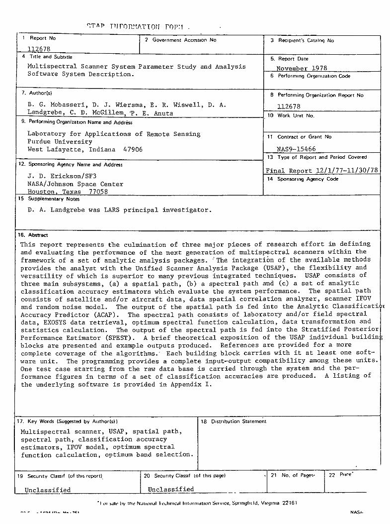
TAP TJ0FOnMATTOrr FOPji
1 Report No 2 Government Accession No 3 Recipienrs Catalog No
112678 4 Title and Subtitle 5- Report Date
Multispectral Scanner System Parameter Study and Analysis November 1978 Software System Description 6 Performing Organization Code
7 Author(s) 8 Performing Organization Report No
B G Mobasseri D J Wiersma E R Wiswell D A 112678 Landgrebe C D McGillem-p E Anuta 10 Work Unit No
9 Performing Organization Name and Address
Laboratory for Applications of Remote Sensing 11 Contract or Grant No Purdue University West Lafayette Indiana 47906 NAS9-15466
13 Type of Report and Period Coveed 12 Sponsoring Agency Name and Address
Final Report 12l77-l13078 J D EricksonSF3 14 Sponsoring Agency Code NASAJohnson Space Center Houston Texas 77058
15 Supplementary Notes
D A Landgrebe was LARS principal investigator
16 Abstract
This report represents the culmination of three major pieces of research effort in defining and evaluating the performance of the next generation of multispectral scanners within the framework of a set of analytic analysis packages The integration of the available methods provides the analyst with the Unified Scanner Analysis Package (USAP) the flexibility and versatility of which is superior to many previous integrated techniques USAP consists of three main subsystems (a) a spatial path (b) a spectral path and (c) a set of analytic classification accuracy estimators which evaluate the system performance The spatial path consists of satellite andor aircraft data data spatial correlation analyzer scanner IFOV and random noise model The output of the spatial path is fed into the Analytic Classificati Accuracy Predictor (ACAP) The spectral path consists of laboratory andor field spectral data EXOSYS data retrieval optimum spectral function calculation data transformation and statistics calculation The output of the spectral path is fed into the Stratified Posterior Performance Estimator (SPEST) A brief theoretical exposition of the USAP individual buildin blocks are presented and example outputs produced References are provided for a more complete coverage of the algorithms- Each building block carries with it at least one softshyware unit The programming provides a complete input-output compatibility among these units One test case starting from the raw data base is carried through the system and the pershyformance figures in terms of a set of classification accuracies are produced A listing of the underlying software is provided in Appendix I
17 Key Words (Suggested by Author(s)) 18 Distribution Statement
Multispectral scanner USAP spatial path spectral path classification accuracy estimators IFOV model optimum spectral function calculation optimum band selection
19 Security Classif (of this report) 20UScu a ssif (of this page) - 21 No of Pages 22 Prce
Unclassified
Io0 ale by
-
nclssIfied tv
Me Nti onaN~ 0 I 1 nh ical1i110111idt011
fll~Il~tNASA
glVr2
SCrvice Spi Ingfaidd Virginia 221I6 1
TABLE OF CONTENTS
Page
List of Figures ii
List of Tables iv
1 Introduction 1
2 Scanner Parameters Analysis techniques 7
3 The Unified Scanner Analysis Package Block Diagram 59
4 Users Guide to USAP 70
5 Summary 93
6 References 98
Appendix I i 100
LIST OF FIGURES
Page
Figure 1 Classification Performance vs Spatial Resolution 5
Figure 2 RMS Error of Proportion Estimates vs Spatial Resolution 5
Figure 3 Classification Performance vs Noise Added for 30120 Meter Resolution 6
Figure 4 Block Diagram of the Unified Scanner Analysis Package
Figure 5 Allocation of a Measurement Vector X to an Appropriate
Figure 6 A Conceptual Illustration of the ACAP Error Estimation
Figure 7 ACAP Classification Accuracy Estimate vs Grid Size for
(USAP) S8
Partition of the FeatureSpace 10
Technique Using Two Features 15
the Test Population Data 16
Figure 8 ACAP Classification Accuracy Estimate vs Grid Size for Graham Co Kansas Data 19
Figure 9 Scanner Spatial Model as a Linear System 27
Figure 10 Scanner Characteristic Function vs Scene Correlation
Adjacent Line Correlation = 65 31
Figure 11 Scanner Characteristic Function vs Scene Correlation Adjacent Line Correlation = 8 32
Figure 12 Scanner Characteristic Function vs Scene Correlation
Figure 13 Scanner Characteristic Function vs Scene Correlation
Figure 14 Scanner Output Classification Accuracy vs IFOV
Figure 15 Scanner Output Classification Accuracy vs IFOV
Figure 16 Scanner Output Classification Accuracy vs IFOV
Adjacent Line Correlation = 1 33
Adjacent Line Correlation = 8 34
Adjacent Sample Correlation = 55 36
Adjacent Sample Correlation = 8 37
Adjacent Sample Correlation = 95 38
Figure 17 Bandlimited White Noise Spectral Density 39
Figure 18 Overall Output Classification Accuracy Variation with Noise and IFOV 42
Figure 19 Realization of a Stratum as the Ensemble of Spectral Samplamp Functions 45
Figure 20 Basis Function Expansion of a Random Process 46
Figure 21 Average Spectral Response -- Wheat Scene 53
Figure 22 Average Spectral Response -- Combined Scene 53
iii
Figure 23 Average nrru4tfon Bnd 1 Wheat Scene 56 Figure 24 Average Infornation Bqnd -Combned Ste 56
Figure 25 Average Informatiq Bande7 Wheat Scee 57
Figure 26 Average Infonatiopn 1i4d 7 iombnSsc e 57 Figure 27 The Block Diagvam of the Unified Scanqxxr Anaiysis
Figure 28 Eigevector 1
Package 4USAP) 60 90
Figure 29 Eigenvector 2 0-
Figure 3a Eigenvector 3 91
Figure 31 Eigenvector 4 9i
iv
LIST OF TABLES
Page
Table 1 ACAP and LARSYS Performance Comparison 17
Eigenvectors and Estimates of the Classification
Table 2 ACAP and LARSYS Performance Comparison Simulated Data 17
Table 3 Test of the SPEST Error Estimate 24
Table 4 Variation of Estimates 25
Table 5 Spectral Bands for Wheat Scene 52
Table 6 Spectral Bands for Combined Scene 52
Table 7 Modeling of the Wheat Scene 54
Table 8 Modeling of the Combined Scene 54
Table 9 Average Information for Wheat Scene Bands 55
Table 10 Average Information for Combined Scene Band 58
Table 11 Order of Preference of Spectral Bands for the Wheat and Combined Scenes 58
Table 12 Error Matrix for Cross Correlation Function Approximashytion Between Channels 2 and 8 64
Table 13 ACAP Sample Output 83
Table 14 SPEST Sample Output 84
Table 15 CORRELAT Sample Output 86
Table 16 SCANSTAT Sample Output 87
Table 17 Eigenvalue and Mean-Square Representation Error for the Data Set 88
Table 18 SPTES and SPEST Sample Output Using the First 4
Accuracy 92
Cl- Multispectral Scanner System Parameter Study and
Analysis Software System Description
1 INTRODUCTION
The utilization of sensors on earth orbiting platforms as the main
element of an Earth Observational System has undergone substantial
growth in recent years ERTS-l (Landsat-l) followed by Landsat-2 and
-3 have proven exceptionally successful in collecting data to help
monitor the Earths resources
The principal data collection unit aboard the first three Landsats
is the multispectral scanner known as MSS Although this scanner has
been providing data with a quality which exceeded most prelaunch
expectations it has been clear from the beginning that MSS does not
represent the ultimate in multispectral instruments more advanced
instruments providing greater detail would be needed as the user community
begins to become familiar with the use of such space data
The design of a multispectral scanner is a very complex matter
many different interacting factors must be properly taken into account
Currently operational systems such as MSS have been designed primarily
using subjective judgements based upon experience with experimental
data In designing a scanner the use of empirical methods at least in
part is essential Each of the large collections of scenes which a
given scanner will be used upon is a very complex information source not
enough is known to make a simple (or even a complex) model of it by
which to make the design of a scanner a simple straightforward exercise
of a mathematical procedure
And yet more is known than when MSS was designed and it is imporshy
tant to be able to carry out future designs on a more objective basis
than in the past Thus the purpose of the present work is the developshy
ment of appropriate mathematical design machinery within a theoretical
framework to allow (a) formulation of an optimum multispectral scanner
The work in this report was done under Task 22C1 Multisensor Parametric
Evaluation and Radiometric Correction Model
2
system according to defined conditions of optimality and (b) an ability
for convenient manipulation of candidate system parameters so as to
Permit comparison of the theoretically optimum designs with that of
practical approximations to it
In order to deal with the complexity of the design situation the
first step is to determine a suitable set of parameters which adequately
characterize it but is not so large as to be unmanageable It has been
observed [i] that there are five major categories of parameters which
are significant to the representation of information in remotely sensed
data They are
1 The spatial sampling scheme
2 The spectral sampling scheme
3 The signal-to-noise ratio
4 The ancillary data type and amount
5 The informational classes desired
Thus it is necessary to have present in the design machinery some means
for evaluating the impact of change in parameter values in each of these
five categories
Such a scanner design tool has been assembled in the form of a
software package for a general purpose computer Each of the parts of
this package called Unified Scanner Analysis Package (USAP) has been
carefully devised and the theory related to it fully documented [2 3 4 51
The goal of this report is to provide a documentation and description of
the software In constructing this documentation it was a~sumed that this
package will be useful for sometime into the future however it was also
assumed that it will only be used by a small number of highly knowledgeshy
able scientists
Section 2 recaps the theoretical concepts behind some of the primary
These are divi7ded into (a) scanner spatial charactershycomponents of USAP
istics modeling and noise effects (b) optimum spectral basis function
calculations (c) analytical classification accuracy predictions
3
(d) stratified posterior classification estimation and (e) an information
theory approach to band selection Although (e) is not a part of the
USAP system the results from this approach are helpful in understanding
the scanner design problem
Section 3 shows the integration of the above modules into the
software system Section 4 is the users guide to USAP describing the
required inputs and the available output products A listing of all
programs is provided in the appendix
The work which led to USAP was immediately preceded by a simulation
study of possible parametric values for the Thematic Mapper a new
scanner now being constructed for launch on Landsat-D in 1981 The
purpose of this simulation was to compare the performance for several
proposed sets of parameters We will conclude this introductory section
by briefly describing this work because it provides useful background
and serves well to illustrate the problem A more complete description
of this simulation study is contained in [l 6]
The general scheme used was to simulate the desired spaceborne
scanner parameter sets by linearly combining pixels and bands from (higher
resolution) airborne scanner data to form simulated pixels adding
noise as needed to simulate the desired SIN the data so constructed
was then classified using a Gaussian maximum likelihood classifier and
the performance measured The problem was viewed as a search of the
five dimensional parameter space defined above with the study localized
around the proposed Thematic Mapper parameters The scope of the
investigation was primarily limited to three parameters (a) spatial
resolution (b) noise level and (c) spectral bands Probability of
correct classification and per cent correct area proportion estimation
for each class were the performance criteria used The major conclusions
from the study are as follows
4
1 There was a very small but consistent increase in identification
accuracy as the IFOV was enlarged This is presumed to stem
primarily from the small increase in signal-to-noise ratio with
increasing IFOV Figure 1
2 There was a more significant decrease in the mensuration accuracy
as the IFOV was enlarged Figure 2
The noise parameter study proved somewhat inconclusive due to3
the greater amount of noise present in the original data than
desired For example viewing Figure 3 moving frolm right to
left it is seen that the classification performance continues
the amount of noise added is decreased until theto improve as
point is reached where the noise added approximately equals that
already initially present Thus it is difficult to say for
what signal-to-noise ratio a point of diminishing return would
have been reached had the initial noise not been present
4 The result of the spectral band classification studies may also
be clouded by the noise originally present in the data The
relative amount of that change in performance due to using
80-91 jimdifferent combinations of the 45-52 Jm 74-80 vtm
and 74-91 Pm bands is slight but there appears to be a slight
preference for the 45-52 jim band The performance improvement
of the Thematic Mapper channels over those approximating Landsat-l
and -2 is clear however
5 Using spectrometer data it was verified that the 74-80 vm and
80-91 Pm bands are highly correlated
6 Correlation studies also showed that the range from 10-13 Pm
is likely to be an important area in discriminating between earth
surface features Further it is noted that the absolute
calibration procedure described above results in a global
atmosphere correction of a linear type in that assuming a
uniform atmosphere over the test site the calibration
procedure permits a digital count number at the airborne
scanner output to be related directly to the present reflectance
of a scene element
The noise level in the original AC data was equivalent to about 005 NEAp
on the abscissa See Reference [ll
-----------------
5
10shy
-815 NDakota
Reflective Emissive IFOV Wm
Figure 1 Classification Performance vs Spatial Resolution
10 ---- 76 Kansas 0 815 U Dakota
0 30tO 40120 5012D 6012 80
ReflectiveEmrssive IFO( m) LANDSAT 2
Figure 2 RMS Error of Proportion Estimates vs Spatial Resolution
Nois Aded (EAPor4~c610c
geo
DL -Mshy7 0 or D2 D3 (x -0o6f
7
2 SCANNER PAPAMETERS ANALYSIS TECHNIQUES
Based upon the parametric approach introduced above the development
of a parametric scanner model must give explicit concern for the spatial
spectral and noise characteristics of the systems This is what has been
done in the Unified Scanner Analysis Package (USAP) shown in Figure 4
USA is composed of two distinct subsystems The spatial aspect of it
contains (a) a data spatial correlation analyzer (b) a scanner IFOV
model and (c) a random noise model The spectral techniques are capable
of producing an optimum spectral representation by modeling the scene as
a random process as a function of wavelengthfollowed by the determination
of optimum generalized spectral basis functions Conventional spectral
bands can also be generated Also studied was an information theory
approach using maximization of the mutual information between the reflected
and received (noisy) energy The effect of noise in the data can be
simulated in the spectral and spatial characteristics Two different data
bases are used in the system The spectral techniques require field
spectral data while the spatial techniques require MSS generated data
aircraft andor satellite The system performance defined in terms of
the classification accuracy is evaluated by two parametric algorithms
A detailed system description and users guide is presented in Sections 3
and 4 In the following the theoretical ideas behind the five major
elements of USAP are discussed
21 Analytical Classification Accuracy Prediction
Throughout the analysis of remotely sensed data the probability of
correct classification has ranked high among the set of performance indices
available to the analyst This is particularly true in a scanner system
modeling where generally the optimization of various system parameters
has as its prime objective the maximization of the classification accuracy
of various classes present in the data set
The estimation of the classification accuracy is fairly straightforshy
ward if Monte-Carlo type methods are employed In system simulation and
modeling however such approaches are generally a handicap due to their
Figure 4 Block Diagram of the Unified Scanner Analysis Package (USAP)
LARSYS CORELAT SCANSTAT
MSS Image Data Spatial Statistics statistics Noise Data Retrieval Correlation IFOlV Model
M(Satelliteod [or AC) In l zeA
A P~
SAnalytic
AClassification - Accuracy -Pc Predictor
Spectral Statistics
SPEST
Stratified Posterior A
Performance
Estimator
EXPSYS SPOPT SPTS
Opt Spect Data TransformationLab or DaIt Spectral Data Optimum
Field Retrieval Ensemble Sample Spectral Functions [ and
Band Function Statistics Ca eulationSpectral Thaid Data Construction - Calculation
Band
Specification
Implies path for spectralspatial statistics
Implies path for data or spectral functions
c
9
heavy dependence on an experimental data base the availability of which
can be limited due to a variety of reasons What is required therefore
is a parametric classification accuracy estimator for a multiclass
multidimensional Gaussian Bayes classifier This procedure should require
the class statistics mean vectors and covariance matrices as its only
input and produce a set of probabilities of correct classification
This technique has been developed tested implemented and comprehensively
reported [2] The following is a summary of the method and some results
The probability of Error as an N-Tuple Integral
The classification of a multidimensional observation vector into
one of M populations is conceptually identical to the binary case Let
0 M and N be the feature space number of classes and the dimensionality
of Q respectively The procedure is to divide 2 into M mutually disjoint
sets Pi and to assign each feature vector to a set in accordance with -
an appropriate rule This is illustrated in Figure 5 Let Zi i = 1
2 M partition S1in R The Bayes risk is defined as
R = i J P(m) Ci f-Xlw) dX 1~ Z J=l
I
is the cost of deciding w1 where w is true In the case where
C=0 for ij and C=1 for ij R is the probability of error iJ 1
where C 13 i1
Among all possible choices of Z the Bayes rule partitions Q into1
Z=Z such that R=R is the the minimum probability of error Assuming1 1
that the population statistics follows a multivariate normal law the
optimum Bayes rule is as follows [7]
X a W3 if W lt W Vi j - 1 2 M
where
Wi = (X- i)T [i-1 (X-_u + ln[iZ-21n P(o)m
i0
~wo2 ~~WM
Allocation of a Measurement Vector X to an Appropriate Partition
F-igure5 of the Feature Space
with
X = observation vector
= mean vector for class w (2)
= covariace matrix for class 1
P( i) = apriori probability for i
The error estimate based on direct evaluation of Eq (1)exhibits all the
desired-properties outlined previously
The evaluation of multiple integrals bears little resemblance to
their one dimensional counterparts mainly due to the vastly different
domains of integration Whereas there are three distinct regions in one
dimension finite singly infinite and double infinite in an N dimensional
space there can potentially be an infinite variation of domains The
established one dimensional integration techniques therefore do not
carry over to N dimensions in general Hence it is not surprising that
no systematic technique exists for the evaluation of multivariate integrals
except for the case of special integrands and domains [8] The major
complicating factor is the decision boundaries defined by Eq (2) P is
defined by a set of intersecting hyperquadratics Any attempt to solve
for the coordinates of intersection and their use as the integration limits
will be frustrated if not due to the cumbersome mathematics because of
impractically complicated results
In order to alleviate the need for the precise knowledge of boundary
locations and reduce the dimensionality of the integral a coordinate
transformation followed by a feature space sampling technique is adopted
The purpose of the initial orthogonal transformation of the coordinates
is an N to 1 dimensionality reduction such that the N-tuple integral is
reduced to a product of N one dimensional integrals Let the conditional
classification accuracy estimate Pc be the desired quantity Then
the transformed class w statistics is given by
12
j = 1 2 M (3)
-3-S = 0T 0
where 0 is the eigenvector matrix derived fromi Naturally in each
transformed space Ti(Q) wi has a null mean vector and a diagonal
covariance matrix
The discrete feature space approach is capable of eliminating the
If 0 is theneed for the simultaneous solution of M quadratic forms
continuous probability space a transformation Ti is required such that
can be completely described in a nonparametric form therebyin TiQ) r1 1
bypassing the requirement foran algebraic representation of P This
desired transformation would sample Q into a grid of N-dimensional
hypercubes Since the multispectral data is generally modeled by a
multivariate normal random process a discrete equivalent of normal
random variables that would exhibit desirable limiting propertiesis
Let ynBi (n p) be a binomial random variable with parametersrequired
n and p The x defined by
Yu- npx Yn 0i 2 n (4)
converges to xN(O 1) in distribution [91 ie
lim F (X) - - F(x)n
The convergence is most rapid for p= then
(yn - n2)2 (5)n
13
The variance of xn is set equal to the eigenvalueof the transformed Yi by incorporating a multiplicative factor in Eq (5)
The segmentation of b a union of elementary hypercubes makes
nonparametric representation of P and its contours feasible Following1
the orthonormal transformation on o and sampling of 2 accordingly each1
cells coordinate is assigned to an appropriate partition of r This
process is carried outexhaustively therefore FI can be defined as a set
such that
r = ux x eli (6)
once the exhaustive process of assignment is completed the integral of
f(Xjwi) over Fi is represented by the sum of hypervolumes over the
elementary cells within P The elementary unit of probability is given by1
61 62 6N
f f (Xi) = 2 f (xli i ) dN T f (x 2 lo i ) d 2 2--2 f (xNIwi) dN
C -61 62 -N
2 2 2 (7)
where C is the domain of a sampling cell centered at the origin and 6
is the width of a cell along the ith feature axis The conditional
probability of correct classification is therefore given by
c Il+ 61 c2+ 62
Pcli - T (x i (x-l2) (C)dx2J f jw) (C)dx x c -6 2c -61
2 2
(8)
c +6 n n
c 2-- f (xNIwplusmn) II(C) dxN
c -6 n n
2
with overall classification accuracy given by
14
M
p P(m) P 1W (9)bullC I
where
1 if Cc (10)ii(C) =
0 otherwise
C = The domain of an elementary cell
Figure 6 is a geometrical representation of Eq (8)
Experimental Results
The analytic classification accuracy prediction (ACAP) has been
Two examples are repeated hepethoroughly tested and documented [2]
The first experiment investigates the performance of the estimator vs
Small to moderate range ofgrid size ie number of cells per axis n
Figure 7 n is required if computation time is to remain realistic
vs n for three classes having some hypotheshyshows the variation of Pcjw c1
The main property of the estimator istical statistics in 3 dimensions
its rapid convergence toward a steady state value thereby alleviating
the need for excessively fine grids and hence high computation costs
The data collected over Graham County Kansas is used to perform
a comparison between the ACAP algorithm and a ratio estimator such as
LARSYS The results are tabulated in Table 1
ff(x)
f(x~lQl)
xl
Figure 6 A Concentual
Illustration of the ACAP Error Estimation
Technicxue Using
Two Features FIEU
100C L A 1- CLASS I s -- 2- CLASS 2S
3- CLASS 51 r 110 0- OVERALL I CA as T I A
C 7S
C
PC
T So CHERNOFF BOUND- 447
ss tI1II
4 8 10 12 14S 7 9 11 15
NO OF CELLS PER RXIS
Figure 7 ACAP Classification Accuracy Estimate vs Grid Size for the Test Population Data 9
17
Table 1 ACAP and LARSYS Performance Comparison
Class No of Points LARSYS ACAP
Bare Soil 443 659 783
CornSorghum 99 899 910
Pasture 1376 984 950
Wheat 459 948 939
Overall 2377 872 896
The comparison of ACAP and LARSYS results from Table 1 is inconclusive
In some cases the difference is negligible (corn) and in some significant
(bare soil) Examination of the data statistics revealed that the
assumption of normality does not hold throughout the populations statistics
This problem can be rectified by simulating random Gaussian data having
identical statistics with the real data hence assuring the normality
assumption Repeating the LARSYS and ACAP procedures produces a new set
of classification accuracies Table 2
Table 2 ACAP and LARSYS Performance Comparison Simulated Data
Class LARSYS ACAP Accuracy Difference
Bare Soil 778 783 05
Corn 912 910 - 02
Pasture 953 951 02
Wheat 942 939 02
Overall 896 896 0
The differential between ACAP and LARSYS results has been narrowed
considerably ranging from a high of 05 for bare soil to 0 for the
overall classification accuracy Two conclusions can be drawn from the
results of this experiment First the ACAP and Monte Carlo type
classifiers produce practically identical results if the underlying
assumptions are satisfied (eg normality of the statistics) Second
and more revealing is the fact that the results of the ACAP processor
indicated an upper bound for the classifability of bare soil had
18
its statistics been Gaussian This result is a direct property of ACAPs
data independence Figure 8 is the ACAP estimator vs n for Graham Co
data
The above selected experiments and others reported in the biblioshy
graphy establishes ACAP as a viable and necessary tool in any analytical
remote sensing data collection system modeling and simulation when the
performance index is defined as the probability of correct classification
22 Stratified Posterior Classification Performance Estimator
The second classification accuracy estimator to be presented here
(SPEST) is based on the maximization of the aposteriori probability
associated with each sample This formulation is closely related to
the maximum likelihood principle used in the ACAP The distinction
arises in the determination of integration domains Where in ACAP a
deterministic grid was set up to sample the feature space SPEST uses
an internally generated random data base and assigns the feature vector
to the appropriate class via the maximum aposteriori principle Due to
the different approaches adopted the statistical properties of the
estimators could be substantially different although no major study has
yet been carried out It has been observed however that the SPEST
algorithm is somewhat faster than the ACAP in selected cases The
approach here is similar to that described in Moore Whitsitt and
Landgrebe [10]
1 2 3 MLet X be an observation from one of M classes wi i =
with a priori probabilities P The maximum likelihood decision rule can 1
be stated as follows Assign X to the class w k if
P(ikIX) = max P(wiX)JX) i
This rule partitions the observation space Q into subregions FI 12 PM
corresponding to the classes il ()2 M respectively Define the
indicator function as
C 100-U
A
4 - - - 4 - - 4 - 4 - -- 4 - - -S4 ~_ ---- 4- --- -4
FI ~~~
N 4
R C I- CLASS 1 C 2- CLASS 25- CLRSS 5 R 4- CLASS 4 C 0- OVERRLL Y
PSC
T ) 1
7S I I 4 8 10 12 14 16
s 7 9 11 15 15 17
NO Or CELLS PER RXIS
Figure 8 ACAF Classification Accuracy Estimate vs Grid Size for Graham Co Kansas Data
kH
20
The probability of correct classification integral is given by
Pc = f M I(x) p(xi) dx (11)
It is desirable to evaluate the probability of correct classification for I
each class as well as the overall probability The performance probability
for the ith class is
Pci = JI i(x) p(xltamp (12)
The overall performance then is
M
p = iPci (13) c i= l1 c
From Bayes rule
P(mijx) p(x)
p(xli) P
hence
Pci = l(x) ptn p(x) dx
p(x) is a mixture density
M
p(x) = X P pjx jl p (
21
Therefore
M P
I - T2 x) P(4)Ix) p(xV1 ) dx (14)Pc1 j=l P i (
Define
Qi(x) = Ii(x) P((i Ix)
Then
f Qi(x) p(xIW) dx
is the conditional expected value of Qi(x) given that X comes from the
class C The estimate
M p N
(15)j=l PN I Qi(xk)j=P5 jJ k=l
is unbiased This estimator is similar to the stratified posterior
estimator described by Whitsitt [10]
To do this a pseudo-random sequence of uniformly distributed random
digits is generated by the power-residue method and is transformed by the
inverse cumulative-distribution-function method to obtain nearly Gaussian
samples These samples are used to fill the elements of the data vector Y
Each vector Y then has expected value 0 and covariance matrix I
By performing the transformation
X = F Y + m (16)J j - -3
22
On the vectors I the random vectors for class j are obtained where 4
is the matrix of eigenvectors required to diagonalize the covariance matrix
of class j rS is the diagonal matrix of eigenvalues and m is the desiredJ
These random vectors are used to evaluate the estimators in mean vector
Eqs (15) and (13)
The term that must be evaluated from Eq (14) is
P p(xlwo)
P(CIx) = YPk P(X_ k Q
k
To evaluate this probability compute P p(xloj) for each class w Choose
the largest value of the product P p(xlm) and divide by the sum P P(XLk)j k
P(x~mk) = exp - (x-mk)T K1 (x - m) (17)
(27F) 2K I
and Kk are the mean vector and covariance matrix respectively for class
k Substituting Eq (16) into (17)
p(xIk) = - exp - T T- Y
2YT r T -1 1 -18 -2 -j Kk (-m-mk) 4 (m-mk) K (m-mk)] (18)
In this form it is not necessary to perform the intermediate computational
step of transforming the data We need only to generate M sets of random
vectors Y with mean vector 0 and covariance matrix I and use them in the
Eq (18)
23
Estimator Evaluation
A subroutine program was written to evaluate classification perforshy
mance by the above method To test the method a three class problem was
constructed The mean vectors for the classes were
1 ]T
S = [-i -i ]T M 2 [0 0
N2 T L3 = [ ]
The covariance for each class was the identity matrix The number of
random vectors generated for each class was 1000 The exact classificashy
tion accuracy as a functidn of the dimensionality can be evaluated for
this case
P = 1 - erfc (fi2)
Pc2 = 1 - 2 erfc (VN2)
P = 1 - erfc (A-2)
P =1 - 43 erfc (AT2)c
t~ -X22
where erfc (a) = edx
and n is the number of dimensions Table 3 contains the results of
evaluating the class conditional performance and overall performance
from one to ten dimensions
To evaluate the variance of the estimates different starting values
for the random number generator were used Twenty trials were used to
evaluate the maximum bound and the standard deviation from the true value
These results are presented in Table 4
For the overall accuracy the estimate is within 005 of the true
value This is certainly sufficient for performance estimation The
Table 3 Test of the SPEST Error Estimatd
Pc1c P P P Pc2 Pc30
1 06915 03829 06q15 05886 06859 03793 07001 05884 2 07602 05205 07602 06803 07671 05116 07700 06829 3 08068 0613j5 08068 07423 08037 06202 08081 07440 4 084-13 06827 08413 07885 08283 06852 08550 07895 5 08682 0-7364 08682 08243 08642 07425 08703 08256 6 08897 07793 08897 08529 08767 07939 08787 08498 7 09071 0814I 0907i 08761 08993 08242 09065 08766 8 09214 08427 09214 08951 09129 08472 09240 08947 9 09332 68664 09332 09109 09193 08809 09360 09120
10 09431 08862 6943i 0924i 09209 09012 09481 09234
25
Table 4 Variation of Estimates
pcl Pc2 Pc3 Pc
1 016 010 017 003 a 033 019 049 005 Bound
2 018 010 014 002 a 036 018 027 005 Bound
3 016 017 017 003 C
046 031 055 007 Bound
4 011 016 015 003 a 025 029 029 005 Bound
5 015 014 012 002 a 031 033 026 004 Bound
6 014 014 010 003 a 026 023 022 006 Bound
7 009 016 012 003 a 027 033 027 005 Bound
8 013 013 012 003 025 036 023 006 Bound
9 013 014 012 002 a 026 031 021 004 Bound
I0 009 012 009 002 a 016 024 019 005 Bound
a = standard deviation
Bound = maximum difference between estimate and true value over 20 trials
26
class conditional estimates are less reliable but are sufficient to
observe trend in the performance due to individual classes
23 Scanner Spatial Characteristics Modeling
The multispectral scanner represents themost important element in
a remote sensing data gathering system Therefote an understanding of
the signal flow through this subsystem is essential As data is processed
through the scanner its statistical properties undergo a transformation
This in turn will alter the population separabilities and hence the
classification accuracies The comparison of this quantity at the scanner
input and output and observationof its variation with the system parashy
meters sheds considerable light on the overall system design Since the
Bayes Ppectral classifier depends solely on the population of spectral
statistics methods need to be developed that relate the scanners input and
output statistics A complete derivation of such relationship is given
in Appendix A of [2] A summary follows
Scanner Characteristic Function
Figure 9 is a basic block diagram of the scanner spatial model where
f through fN are N stochastic processes corresponding to N spectral
bands and h(xy) is a two dimensional PSF In particular where the Landsat
scanner is concerned the assumption of a Gaussian shaped IFOV has been
widespread Let f(xy) g(xy) and h(xy) denote the input and output
random processes associated with any two matching bands and the scanner
PSF respectively It is well known that the above quantitfes are related
by a convolution integral
Jg(xy) f f(x-1y-A 2 ) h(XV1 2) d IdX 2 (19)shy
it follows that
S(UV) SIf(uv)IH(uv)l2 (20)
27
n(xy)
f2 h(xy)+ 92
f- _-+ gN
Figure 9 Scanner Spatial Model as a Linear System
28
where S(uv) is the spectral density of the appropriate random process
and H(uv) is the two dimensional Fourier transform of the scanner PSF
Let M(uv) = IH(uv)12 afd m(Tn) its inverse transform Then the output
spatial autocorrelation function is given by
R (Tn) = Rff(Tn) m(Tn) (21)
In order to obtain specific results the following assumptions are
invoked (a) exponential data spatial correlation (b) Gaussian IFOV
PIT I Rff(Tn) = 011 rn 0 1 2
(22)
2 2 h(xy) = c1 e - e2
r r 0 0
=-a =-b where px = e and py = e are the adjacent sample and line correlation
coefficients respectively r is the scanner PSF characteristic length
O in-pixels and c1 a constant providing unity filter gain Using the
separability property of the functions inv6lvedi
R g(TI) = Rff(T-X-) m(x) dx f Rff((Th-y) rn(y) dyJ where
c 2 2 r0 2 2 n
m(rr) = 2 e 2r 2e 2- 2 (23)
0 0
carrying out the integration the scanner characteristics funation is
given by
29
2 a222 lar a r
_- -aT +a
W (TIab) = Q(ar --L-) + e Q(ar +U)X 0 0
bt~rr 2or Qb l
o + o +bf
2Lr- Q(br2Q(br ) (24)e
where
2x
Q(x) = e 2
The spectral statistics is a subset of the spatial statistics hence
W (00ab) defines the ratio of the variance at the scanner output to s
the corresponding input quantity
The output crosscovariance terms can be similarly derived Let
the crosscorrelation function between bands i and j be defined as
Rff (T) = rffaf of e-aeIrI -biiI (25)213 1J 1 j
where rf f is the spectral crosscorrelation-coefficient at the input
such that Irff I lt 1 aij and bIj are defined similar to a and b with
the additional channel specification Following the previous technique
it follows that the crosscovariance term between channels i and j is
given by
Rggj (00) = rffoff off Ws(00aijb)ij (26)
1J 1 J i i ij 12 2
30
The corresponding crosscorelation coefficient follows
W (00a ibi) Sgigj - rff
w 2(00aii~bii) WbOOa b) i s si 33 33
Therefore the band-to-band correlation coefficients are identical at
input and output provided the spatial auto and crosscorrelashythe scanner
tion function at the input are equivalent ie aiiaij biib ij A
closed expression can also be obtained for a rectangular PSF defined by
I~o Ix lyl o2
(28)h(xy) =
0 elsewhere
the corresponding characteristic function is given by
-a r
(i1 - ) X -lW (OOa)= 2 l-e 110
s O aiii ar ar I 0 11 0
-br
br2 (I l-er 110 -) (29)
ii o ii 0
Eq (24) and Eq (29) are plotted in Figures10 through 13 for different
as a running parameter The scene correlations with the IFOV = r0
of either PSF is the increasing outputuniversal property exhibited by Ws
variance reduction as IFOV is increased This property hasbeen widely
verified experimentally Comparison of Figumsll and 13 indicates that
for the same IFOV a Gaussian shaped IFOV causes a heavier variance
a rectangular PSFreduction in a spectral band than that of This
property can potentially produce a higher separability among the populashy
tions as the signal is processed through the scanner electronics
W 1 GAUSSIAN SCANNER PSF EI
H INCREASING IFOV (i PIXELSTEP)T 8
I N G7
F A C T0 R
2 2 N 8
0 1 is 2 6 5 5 5 4 5 s S 5 e 7 5 a s 96 95
ADJACENT SAMPLE CORRELATION
Figure 10 Scanner Characteristic Function vs Scene Correlation Adjacent Line Correlation = 65
W GOUSSIRN SCANNER PGF E I G H
N
T 8INCREASING IFOV (I PIXELSTEFP
C
R
FA
T0
04
1 15
2
2s
5S
4 8 4S 5 75
ROJPCENT SRMPE CORRELATION
8 85 S
Figure 11 Scanner Characteristic Function vs Scene Correlation Adjacent Line Correlation = 8
E 1 GRUSSIRN SCANNER PSF
H T8 I N G F A
INCREASING IFOV (1 PIXELSTEP)
T
R
4
2
1
1
15
2
25
5s
4 S 7
4S 55 8s 7S
ADJACENT SRMPLE CORRELATION
85
9 95
Figure 12 Scanner Characteristic Function vs Scene Correlation Adjacent Line Correlation = 1
1 RECTANGULAR SCNNER PSF
I 9 rINCREASINGH IFOV (I PIXELSTEP)
T I N G
F A C T 0
4
2
IA 2 4 68 7 8 1s 2S 5s 4S SS s 7S 85 9s
ADJACENT SANPLE QORRELATION
Figure 13 Scanner Characteristic Function vs Scene Correlation
Adjacent Line Correlation = 8
35
The input-output statistical relationship just developed along with
the analytic classification accuracy predictorprovide the two basic
tools required for a parametric evaluation of the MSS performance under
varying operating conditions As an illustration three hypothetical
classes with some prescribed statistics are specified at the scanner
input Three different sceneswith adjacent sample correlations of 05
085 and 095 are considered The scanner characteristic function
produced a set of transformed statistics at the output followed by the
estimation of the conditional classification accuracies using ACAP for
8 different IFOVs The results are plotted in Figuresl4 through 16
Two main properties stand out First is the improvement in class
separability as the IFOV is enlarged This is true in all the cases
The rate of improvement however is strongly correlated with the scene
spatial correlation The lower the input scene correlation the higher
the classification accuracy improvement per IFOV step This property
is brought about by the characteristics of Ws where one step increase
in IFOV size produces a greater variance reduction for a low scene
spatial correlation than a similar increase would cause in a highly
correlated scene
The scene spatial correlation plays a significant role in the overall
system performance which is not readily obvious One of the well
known properties of linear systems with random inputs is the reduction
of the output varianceinput variance ratio as the point spread function
(PSF) is widened In this section it has been shown theoretically that a
third factor in this reduction is the spatial correlation structure of
the input stochastic process Specifically with everything else fixed
a process having a moderate scene correlation will undergo a tighter
clustering around its mean than an otherwise identical process with a
highly correlated spatial characteristic On the extreme side of the
correlation scale with a small pixel-to-pixel correlation the ratio of
the output variance to the corresponding input quantity is very negligible
Consider a bandlimited white noise process with a spectral density
shown in Figure 17where W is the bandwidth and No2 the two sided specshy
0 1001
I go
C Rq T S86
N
P8r C C U 7 153 R R C Yr 70
1
I1- CLSSS
2- CLRSS
I
C T 85
3-0-
CLRSS 5 OVERRUL
SCFRNNER IFOV IN HIGH RESSLUTION PIXELS
Figure 14 Scanner Output Classification Accuracy vs Ifl Adiacent Sample Correlation = 55w
C 100
L R S I F
Ao
T1 85
0 N
8 0f1C C U 75 R C I- CLASS I Y 70
2- CLASS 2 F 3- CLASS 5C
0- OVEWILLT BE
742
SCANNER IFOV IN HICH RESOLUTION PIXELS
7Figure 15 Scanner Output Classification Accuracy vs IFONAdjacent Sample Correlation = 8
10c LAS 9- O SI F
CC 2- CLASS 2
1 85 T 3- CLA~SS 5 0 0- OVERALL
N
A80 C
UR
C 7S
C Y 70
P
T GS
2 4 8
SCRNNER IFOV IN HIGH-RESCUTION PIXELS
Figure 16 Scanner Output Classification Accuracy vs IFOV Adjacent Sample Correlation = 95
00
39
No2
-2gW 27W w
Figure 17 Bandlimited White Noise Spectral Density
tral density As W increases the adjacent pixel correlation in the
scene decreases The increase in W however is accompanied by a
decrease in No2 if this process is to remain physically realizable
(finite energy) Under a finite energy constraint therefore as W-shy
No2-- 0 In the limit the energy content of the output random process
will be nil
Random Noise
Additive random noise entered at various stages of a scanner system
can degrade the overall system performance substantially The noise can
be classified into two broad categories external and internal A
major source of external noise is atmospheric in nature mainly due to
absorption (eg water vapor) and scattering The detector and quantishy
zation noise comprise the major component of the internal noise sources
From a system analysis point of view the latter represents a more tractshy
able and better understood component of the random noise [11] while
the former still awaits further experimental documentation The purpose
of this work is not so much the exploration of the various noise sources
but the integration of its effect within an analytic analysis package
once its characteristics and origin has been determined
can be stated that atmosphericFrom the theoretical results obtained it
noise in the uplink path at least has negligible degrading factor
compared with the detector and quantization noise Let f(xy) Nf(xy)
f(xy) and Nf(xy) be the input random process input additive white
40
noise the output random process and the noise component of the output
signal respectively then
f-(xy) = f(xy) h(xy) (30)
N (xy) = Nf(xy) h(xy) (31)f
Define
(SNR)f = Var f(xy)1Var Nf(xy)l (32)
(SNR) -= Var f(xy)Var N (xy)) (33) f f
Recalling the functional dependence of Ws on the input scene spatial
correlation it follows that the ratio of the variance of a white noise
process at the scanner output to the corresponding input quantity is of
the order of 5 to 10 higher or lower depending on the IFOV size
Therefore
Var f(xy) lt Var f(xy)l (34)
Var N (xy)l ltlt Var Nf(XY (35)f
hence
(SNR) f gtgt (SNR)f (36) f
It then follows that the noise component of the output process prior to
casesdetector and quantization noise is negligible in most
In order to observe the effect of noise on the scanner output class
separability the test class statistics were modified to exhibit the effect
of random noise The assumed properties of the noise are additive
white and Gaussian Let F-(xy) )e the signal to be teJmeterud to
Earth
41
f(xy) = f(xy) + N (xy) (37) f
the statistics of f(xy) and f(xy) are related by
+ Y (38) r~f -N
f
the simple addition is due to the signal and noise independence Assuming
a zero mean N the mean vector are identical ie f
E ffj = E f-)
Among the four assumptions about the noiseits Gaussian property is the
weak link due to the Poisson distributed detector noise and uniformly
distributed quantization noise Relaxing the Gaussian noise assumption
however would mean the design of an optimum classifier for non-normal
classes and evaluation of its performance A task that would complicate
matters considerably Due to the relatively insufficient documentation
of the characteristics of random noise in multispectral data the initial
Gaussian assumption is adhered to
Following the adopted SNR definition three different noise levels
are considered and the corresponding overall classification accuracies
for the three previously used test classes are estimated Figure 18 is
the variation of P vs IFOV with SNR as the running parameter For a c
fixed IFOV P increases with increasing SNR For a fixed SNR P c c
increases with increasing IFOV size These illustrations have shown
that with a proper coupling between the ACAP and the scanner characteristic
function the progress of the population statistics through the system
can be studied on an analytical and entirely parametric basis The
accompanying classification accuracies can measure the designers success
in selecting the spatial andor spectral characteristics of a Multispectral
Scanner System
C S LSs
1 80 SNR-50 0BF 8 I C R
I 7 -0 N
T
37cent0 U
C
R
C Y ( 6s-- SNR=10 0B P 6 C T
2 4 6
SCANNER IFOV IN HIGH RESOLUTION PIXELS
Figure 18 Overall Output Classification Accuracy Variation with Noise and IFOV
43
24 Optimum Spectral Function Research
In earth observational remote sensing much work has been done with
extracting information from the spectral variations in the electromagnetic
energy incident on the sensor Of primary importance for a multispectral
sensor design is the specification of the spectral channels which sample
the electromagnetic spectrum An analytical technique is developed for
designing a sensor which will be optimum for any well-defined remote
sensing problem and against which candidate sensor systems may be compared
Let the surface of the earth at a given time be divided in strata
where each stratum is defined to be the largest region which can be
classified by a single training of the classifier Each point in the
stratum is mapped into a spectral response function X(X) as in Figure 19
That is if one observes a point in the stratum with the sensor then the
function X(A) describes the response variations with respect to the
wavelength X The stratum together with its probabilistic description
defines a random process and the collection of all of such functions
X(X) which may occur in the stratum is called an ensemble
The general concept of a pattern recognition system in this applicashy
tion requires that if each X(X) is to be classified by a classification
algorithm this can be accomplished by first measuring a finite number
of attributes of X(A) called features This is the function of the
sensor system as depicted in the upper left portion of Figure 20 where
X1 X2 X are the values of N features for a given X(X) It
may be viewed as a filtering operation on X(A)
For example on the right portion of Figure 20 the function of MSS
of the Landsat satellites is illustrated In this case a number proporshy
tional to the average energy in a wavelength interval is reported out by
the sensor for each of four wavelengths Mathematically this may be
expressed as
Zn f X n)(X)dX n = 1 2 3 4
44
Next we must consider what would constitute an optimum sensor We
first note that in general the sensor may be used over any part of the
earthb surface at anytime and for many different applications (sets
of classes) Therefore the sensor must be optimized with respect to the
entire set of strata represented by these cases As a result of the large
size of this set and the fact that its statistical description is not
known we will optimize the sensor with respampct to its signal representashy
tion characteristics The fX(A) each contain information Useful to the
classifier we require of the sensor design that for a given N a maximum
of this information which was in X(A) still be present in X Since n the specific nature of this information is not known a priori we can
only assure that this will be the case for any stratum if X(A) is
recoverable from fX I n
Let X(A) be the result of attempting to reconstruct X(A) from X n
A fidelity criterion which is useful in this instance is
= f[X(X) - x(X)] 2 dA (39)
the so called mean square error or mean square difference between X(X)
and X(A)
It is known [12J thata reconstruction scheme which minimizes C for
a given N is
X(A) = XI1 (A) + X2 2(A)+ + +n(A)
N X + (A) (40)
n=l
provided that the n(A) are orthogonal over the wavelength interval of
interest ie
S m(X)n(X) d) = 0 m n (41)
Stratum The Ensemble
A
A
A
Figure 19 Realization of a Stratum as the Ensemble of Spectral Sample Functions
Figure 20 Basis Function Expansion of a Random Process
x(AxSensorI X2
XN
A A
I
I
I
I-- i
X1lA) =Xl~il l +X2I2A]I+
4SNA)
^
47
and the X are calculated byn
X = X(x) Mn(3dA (42)
Note for example thatthe Landsat example of Figure 20 satisfies
these conditions In the lower right of Figure 20 is depicted the
result of such a reconstruction for the Landsat example
While use of Eq (42) in the case does minimize s with respect to
the choice of values of TX 1 a further improvement may by obtained byn
choosing a set of iIXI which minimizes E Itcan be shown [5 12]
that the set n(X) which accomplishes this must satisfy the equation
U = R(AC) C()dC (43)
where
R(XC) = E[X(A) - m()] [X( ) - m( )]1 (44)
is the correlation function of the random process and m(X) is its mean
value at X
Such a signal tepresentation defined by Eqs (40-44) is known as a
Karhunen-Lo~ve expansion [13] It provides not only for the most rapid
convergence of X(X) to X(X) with respect to N but in addition the random
variables (X are uncorrelated and since the random process is Gaussian n
they are statistically independent Further the only statistic required
of the ensemble is R(XC) This representation of X(X) is therefore
not only optimal it is convenient
A useful generalization of the Karhunen-Lo~ve expansion can be made
Suppose a priori information concerning portions of the spectral interval
are known and it is desired to incorporate-this knowledge into the analysis
A weighting function w(A) is introduced which weights portions of the
interval according to the a priori information As an example measureshy
48
ments were taken over the spectrum and it was observed that there was
considerable variation in the signal in the water absorption bands
around 14 and 18 micrometers This variation was due to measurement
and calibration difficulties rather than being a result of variations
in the scene Therefore the weighting function was set to zero in
these absorption bands This generalization is referred to as the
weighted Karhunen-Lo~ve expansion [5] Eqs (40) (42) and (43) become
N X(A) = x( AsA (45)
i=1l
a (A) = FR(AE) w( ) 4 (E)dE (46)w i f w
x X(A) w() tw (X) dA (47) 1
where the eigenfunction 41 (A) are solutions to the integral Eq (46)W 1
with the weight w(A) The special case where w(A) = 10 for all AcA
reduces the expansion to the original form in Eq (40) (42) (43) and
(44)
The results of having utilized this means of optimal basis function
scheme on spectral data are contained in reference [5] From them one car
see the significant improvement in classification accuracy which decreased
spectral representation error will provide One can also determine the
spectral resolution and band placement needed to achieve such classification
accuracy improvement
25 Information Theory Approach to Band Selection
The ptoblem of selecting a set of optimum windows in the electroshy
magnetic spectrum for observing the reflected sunlight has always been of
considerable interest Depending on the definition of the optimality
different methods have been developed One such approach was shown in
Section 24 using K-L expansion to select an optimum set of basis functions
In this section an information theoretic definition of optimality developed
in [3] is explored
49
Mutual Information and Stochastic Modeling
The reflected energy from the target is detected by the scanner
and corrupted by various noise sources If S is the noise-free signal
Y the observation and N a random disturbance then
Y = S + N (48)
the reduction of uncertainty about S obtained from Y is called the
average or mutual information between the observation and original signal
Since the reconstruction of the reflected signal from the noisy observashy
tion is the highly desirable capability the comparison of such average
information-and selection of these bands with the highest information
content is chosen as-a means of spectral band selection Let
S = (sl s 2 )
and
)Yn =(Yl Y2 Yn
where si and yi are the coefficients of the orthonormal (K-L) expansion
of Y and S then the mutual information between Y and S is given by [3]
T(YS) = - log et (49)
where C and C are the covariance matrices of (yi i = 1 2 ) and
(ni = No2 i = 1 2 ) and No2 is the two sided spectral density of
the additive white noise Equivalently I(YS) can be represented in
terms of the Wiener-Hopf optimum filter impulse response
A-(2
T()= J h(AA) dA (50)
11
50
h(XA) provides an estimate of S from Y with a minimum mean-square error
This relationship however is not a practic d-dethod of evaluating I(YS)
since the actual solution of the Wiener-Hopf integral itself is a nontriyal
task This problem can be circumvented by a discrete state variable
formulation ieshy
s(k+l) = _s(k) + FW(k) ke[Al x2 ] (51)
where
s1(k+l)
s2(k+l)
s(k+l) =
Sn(k+l)
is an (nxn) matrix
r is an (nxl) vector
W(k) = a descrete independent Gaussian
zero mean random process
The formulation of the problem in the discrete domain -provides a practical
way of computing hXX) through Kalman filtering techniques The discrete
version of Eq (50) is given by
I(YS) = - h(kk)
k 6 AA 2 (52)
The discrete nature of this approach makes the evaluation of Eq (52)
considerably more practical than its continuous counterpart This is due
to the fact that the Wiener-Hopf equation is easily solved in only those
cases for which the analytical form of Ks (Au) the signal eovariance
fnnction is fairly simple not likely for most-random processes encountered
51
in remote sensing Since h(kk) is dependent on the parameters of Eq (51)
a concise representation of s(k+l) is needed
The general form of Eq (51) is given as an autoregressive (AR)
model
m1 m2
s(k) = X as(k-j) + I bji(k-j) + W(k) (53) j=l J j1
s(k) = The spectral response at the discrete
wavelength k It is a Gaussian random process
w(k) = zero mean independent Gaussian disturbance
with variance p
(kj) = deterministic trend term used to account for certain characteristics of the empirical data
ab = are unknown constant coefficients to be I i determined
mlm2 = The order of the AR model
The identification selection and validation of general AR models
for the representation of a random process is a well developed technique
[1415] The identification of an appropriate model provides the
necessary parameters required for the evaluation of I(YS) in Eq (52)
The model selection process for a selected number of ground covers has
been carried out [3] leading to the ranking of a set of spectral bands
according to the criterion outlined previously A summary of the
experimental results are given below
Data Base and Model Selection
Two different sets of empirical data are used to demonstrate the
techniques developed here The first set consists of observations of
wheat scenes The second set consists of several vegetation cover
types such as oats barley grass etc For each scene the spectral
responses collected by the Exotech 20C field spectroradiometer are
averaged over the ensemble It is thought the resultant average
52
zspectral response provides a relatively good data set for demonstration
-purposes Figures2l and 22 show the average response for both cover
types
In order that the study be carried out in a context that is relashy
tively realistic for multispectral scanners the spectral response -of
the two data sets is divided into a cnumber -of spectral banids The division
is fairly arbit-rary but each band must contain a sufficient number of
data points to ensure accurate parameter estimation for model identifishy
cation The spectrum is divided into 9 bands from 045 pm to 238 pm
with two gaps in the 134-145 pm and 182-196 -pm range -due to atmosshy
pheric absorption see Tables 5 and 6
Table 5 Spectral Bands for Wheat Scene
Band Number Spectral Wavelength Interval (Pm)
1 045-054
2 054-062
3 062-071
4 071-085
5 085-099
6 099-013
7 113-134
8 145-182
9 196-238
Table 6 Spectral Bands for Combined Scene
Band Number Spectral -Wavelength Interval (pm)
1 045-054
2 054-062
3 062-071
4 071-085
5 -085-098
6 098-112
7 112-130
8 145-18 2
9 196-238
53
s15
10-
S
AX(Uir)0 0 1 2 2S
Figure 21 Average Spectral Response -- Wheat Scene
1I X im)
S
0
0 1 5 FS Rsp2s
Figure 22 Average Spectral Response -- Combined Scene
54
The next step is the identification and validation of models that
would adequately describe the aforementioned spectral responses Three
different models were tested and compared (a) autoregressive (AR)
(b) autoregressive plus a constant trend (AR+C) (c) integrated
autoregressive (I-AR) Following the standard selection and validation
techniques one of the above 3models is selected which describes the
scene most satisfactorily Tables7 and 8 show the selected models for
the wheat and combined scene respectively IAR-2 in Table 8 in a second
order IAR
Table 7 Modeling of the Wheat Sc~ne
Band Order of Model
1 7
2 2
3 11
4 1
5 1
6 2
7 5
8 8
9 6
Type of Model
AR
AR
IAR
AR+C
AR
AR+C
IAR
IAR
IAR
Table 8 Modeling of the Combined-Scene
and Order of Model Type of Model
1 11 IAR-2
2 2 AR
3 11 IAR
4 1 AR+C
5 3 AR
6 1 AR
7 9 AR+C
8 8 tAR
9 1 AR
55
Spectral Band Selection
It was initially stated that the information content of a set of
spectral bands can be used in the selection of an optimum subset Here
the preceding regression analysis will be used to evaluate the mutual
information between the reflected energy and the observed signal in the
9 spectral bands under study
The first step is the computation of the average information in y(k)
the received spectral process about s(k) The reflected spectral scene
response as a function of spectral bandwidth for each band of both
scene types The average information is computed for several values of 2
the noise variance a N Appropriate software is developed to carry out
the calculation of I(YS) Figures23 and 24 show the variation of
I(YS) in nats for the wheat and combined scene in band 1 Similar plots 2 -3are shown for the infrared band 7 Figures 25 and 26 Selecting a a = 10
for demonstration purposes the average information for wheat and combined
scenes are tabulated in Tables9 and 10 for 9 spectral bands
Table 9 Average Information for Wheat Scene I
Band I(YS) nats
1 3450
2 1052
3 2035
4 3000
5 4496
6 3720
7 6031
8 3480
9 5010
56
0
-51080 I(nats)
40--1shy
20shy
a -Io
k 1
1080400
Figure 23 Average Information Band 1 Wheat Scene
s I(nats) 10-5
10
0 40 0 120
20 40 L00
Figure 24 Average Information Band 1 Combined Scene
57
10 - I (nats)
10-5
7510
so
2s 10shy2
o = i0-1 26
n
0 - k 0 100 200
so ISO
Figure 25 Average Information Band 7 Wheat Scene
100 1(nats)
7S 7-5 10 3
0-2
100 200 s0 IS0
Figure 26 Average Information Band 7 Combined Scene
0
58
Table 10 Average Information for Combined Scene Band
Band I(YS) nats
1 4133
2 1617
3 2298
4 4008
5 4573
6 4096
7 7825
8 6415
9 7419
Using the information content of each band as an optimality criterion
the 9 spectral bands can be ranked see Table 11
Table 11 Order of Preference of Spectral Bands for the
Wheat and Combined Scenes
Rank Wheat Scene Band Combined Scene Band
1 7 7
2 9 9
3 5 8
4 6 5
5 8 1
6 1 6
7 4 4
8 3 3
9 2 2
The top 6 highest ranked bands although ordered differently are the
same for both cover types Moreover other than band 1 which is in the
visible portion the remaining 5 are all in the infrared portion of the
spectrum Thus relative to the average information criterion the
infrared portions of the spectrum is generally preferred to the visible
portion since bands 2 and 3 are ranked lowest for both the wheat scene
and combined scene
59
The selection of a subset of the available spectral bands using the
idea of their information content is a new approach in band selection
and requires further investigation to evaluate its optimality in more
concrete terms One of- the most useful optimality criterion is the
selection of these bands that maximize the overall classification accuracy
No -documented relationship exists between the average information contents
of a set of bands and the subsequent class separability It is true
however that such information measure is directly related to the optimum
Weiner filter thereby providing a basis for the optimality of this
ranking technique
3 THE UNIFIED SCANNER ANALYSIS PACKAGE BLOCK DIAGRAM
The identification and development of a set of individual techniques
and algorithms is only the first step toward a complete system simulation
package The usefulness of this package is fully realized only when the
elementary modules are interconnected in a logical and clear fashion The
objective here is the integration of the available processors such that
starting with a raw data base the question of optimum spectral bands
IFOV size and the noise model can be answered with the classification
accuracy as a primary performance index
31 System Structure
One realization of such simulation model was shown in Figure 4 and
is repeated here for convenience in Figure 27 USAP is basically composed
of three distinct parts (a) a spatial path (b) a spectral path and (c) a
means for classification performance estimation In the following
individual software modules are discussed
Classification Accuracy Estimators
There are two classification performance estimators available
(a) the analytic classification accuracy predictors and (b) the stratified
posterior performance estimator
Figure 27 The Block Diagram of the Unified Scanner Analysis Package (USAP)
MS mage
Data
LARSYSData I
RetrievallliteJ
CORELATSpatial - Spatial
Correlationl StatisticsAnalyzer Model
SCANSTAT[Spectral
Saitc Saitc
os
ACAP
Spectral Statistics
Analytic Classification Accuracy Predictor
SPEST
A Pc
Stratified Posterior
Performance Estimator
A Pc
EXOSYS SPOPT SPTES
r
ra
Data Retrieval
SpectralandBand Construction
Spectral Data Ensemble Sample
OptiMum Spectral
Function Calculation
Opt Spect Functions
)0
Data Transformation and
Statistics Calculat[tYV
Band-- --
Specification
Implies path for spectralspatial statistics
Implies path for data or spectral functions
61
Analytic Classification Accuracy Predictor The ACAP algorithm
discussed in Section 21 is the primary processor in evaluating the
performance of a scanner system when the probability of correct classifishy
cation is defined as the primary performance index This piece of
software as shown in its theoretical development requires one major
input in the form of the population statistics In order to facilitate
the operations the format of the statistics deck is chosen to be
identical to the one produced by LARSYS statistics processor although
it contains a considerable amount of redundancy such as field coordinates
These cards are skipped Among other user-supplied information is the
desired spectral bands to be used in the analysis and the-sampling and
grid fineness in the form of number of elementary cells per axis
There is obviously a trade-off between the estimators variance a
decreasing function of the grid size and the computation time If
N is the number of spectral bands and n the number of cells per axis
the per class number of cells to be tested in a set of M quadratic
discriminant functions is nN This exponential relationship calls for
a careful selection of n particularly for a high dimensional space
On the other hand a small variance is very much required property of any
estimator
The relationship between grid structure and the estimators variance
has been covered in detail [2] It was shown that the classification
accuracy obtained using ACAP exhibits a relative independence from n for
n gt 12 This property is preceded by a fairly rapid rise to a steady
state value after which the magnitude of the Pc oscillations is within
05 of the true value or the Monte Carlo derived reference The choice
of n is ultimatamply decided by the user depending on his specific needs
and after some experimentation Initially however a default option of
n = 9 cells per axis is considered to provide quick turn-around time
while keeping the quality of the estimate high The output in addition
to the classification accuracy estimate contains information on the
transformed class statistiamps feature space and sampling grid structure
62
Stratified Posterior Classification Performance Estimator This
is the software implementation of thealgotthm discussed in Section 22
The maximum conditional aposteriori classprobability is the criterion
for classifitation and error estimation purposes The program does
not provide any options and the size of the internally generated random
data is fixed ACAP and SPEST produce differentbut very close results
Spatial Path
Data Base The input data to the spatial scanner model is via the
multispectral image storage tape containing satellite or aircraft
collected data This tape has been reformatted and is compatible with
any LARSYS processor
Data Retrieval The individual software units can access the
available data base through various system support routines or any of
the LARSYS processors
Spatial Correlation Analyzer The determination of the scanner
characteristic function requires a knowledge of the spatial properties
of the input data therefore a class conditional estimate of the spatial
auto and crosscorrelation functions is needed Let f (xy) be a twok
dimensional image of size N x N pixels in the kth spectral band then0 0
the spatial autocorrelation function estimate is given by [16]
No-t No-n
^Rkk(Tn) = C Y Y fk(ij) - k] [fk(i + T j + n) -Vk]i=l j=l
TT1 = 0 1 n -1 (54)
where-pk = Efk(xy)l The multiplicative factor C can be chosen ta be
one of the following
1 (55)CI= (N -T)(N -ii) (
U1(
63
1 C2 =2
if k ts known and C = C1 then ERkk(Tn) = Rkk(Tfn)- If Pk--Ik then
neither selection of C1 or C2 will produce an unbiased estimate The
actual derivation of the mean and variance of Rkk when the mean is
estimated is rather complicated The bias of the estimate in one
dimension is given by [161
N-ITIVar -2 (56)
ERk(T) - R(r) = -R() k + O(No)NN k 0
0 0
From Eq (56) it follows that R( ) is asymptotically unbiased This1
result can be extended to the two dimensional functions provided the
autocorrelation function is separable along each spatial axis In
general the maximum lag n must be chosen such that n ltlt N As a
rule of thumb it is desirable to keep the maximum lag less than one-
This will tend to avoid certain instabilitiestenth the sample size N 0
that can occur in autocorrelation function estimates The across-band
correlation function estimate is obtained using an identical relationship
to Eq (54)
The empirically obtained spatial correlation matrix needs further
processing to be used in the scanner spatial model developed in Section
the experimenshy23 Specifically a Markov correlation model is fitted to
tally obtained lkk(Tr) By invoking the separability assumption for
small lag values
R(rn) R(r) R(n) (57)
where no subscript indicates either auto or crosscorrelation function
Table 12 shows the magnitude of the errors involved in carrying out
this approximation on an aircraft data set The error is expressed as
a percentage of the experimental values An exponentially dropping
function is then fitted to the individual correlation functions along
the sample and line directions The fitting is accomplished using a
64
Table 12 Error Matrix for Cross Correlation Function Appr6ximation Between Channels 2 and 8
100 92 81 69 59 50 44 93 88 78 67 56 48 41
73 71 64 54 44 36 3 R28 48 47 43 36 28 2i 16
30 31 29 24 18 12 08
23 25 24 21 16 12 08
22 24 24 22 19 15 12
100 92 81 69 59 50 44 93 86 75 64 55 46 4
73 67 6 5 43 36 32 R28 48 44 38 33 28 24 71
30 27 24 2 17 15 13
23 21 18 16 13 11 1 22 2 18 15 13 11 1
0 0 0 0 0 0 0 0 22 38 45 18 416 243 0 56- 62 74 23 O 675
28E 0 64 116 83 0 175 238 0 130 172 166 55 20 384
0 16 25 238 187 83 20 0 166 25 318 316 266 166
65
weighted least square approach to the logarithm of R(T) and R(n) The
slope of this linear fit determines the adjacent sample or line
correlation coefficients Specifically let
F(i) = ln R(i) i =0 1 n -l
0
then the parameters of the linear fit CI+C 2xare given by [17]
C = (HT W H) -I HT W F (58)
where
E(i) = 1 = 0 no(59)0
0 i no+lH(i) 2n -l-i = 0o 0O 2n -i
and the diagonal weighting matrix W
(n -1-i) i = 0 1 n - (60)W(i) = a
with a as the weighting matrix diagonal base o lt a lt 1 The weighting
matrix via the control parameter assigns a progressively smaller weight
to R(Tn) for succeeding lag values This weighting is necessary since
the properties of the correlation functions show an increasing deviation
from the underlying assumptions of separability and Markovian structure
for higher lag values
A complete specification of the spatial properties of the available
spectral classes requires determination of
N N + 2 (N-2)
auto and crosscorrelation functions per spatial axis per class where N
is the total number of spectral bands used in the analysis The impleshy
menting software contains various default provisions in case the correshy
66
lation properties of the input data differs considerably from the aforeshy
mentioned assumptions
The user specifies the area to be correlated by a run table entry
run number followampd by the field coordinates In order to perform either
the auto or crosscorrelation operations appropriate spectral bands(s)
need to be specified The maximum lag no in computing R(tn) is also
a variable and is entered as a percentage of the image size in pixels
The value of n is dependent on the size of the area to be correlated 0 ^
Since the magnitude of R(Tn) for Landsat data is generally negligible
for more than 4 or 5 pixels lag n as a percentage can take on small
values for large fields and vice versa
Scanner IFOV Model The scanner IFOV software is the computer
implementation of the scanner characteristic function discussed in
Section 23 The input consists of (a) spectral covariance matrix
(b) spatial correlation matrix along the samples (c) spatial correlation
matrix along the lines and (d) IFOV size in terms of the number of high
resolution pixels A standard LARSYS statistics deck produced by the
statistics processor constitutes the first item The spatial correlashy
tion information in entered through an N x N symmetric matrix the (ij)
element of which
-a Pj = e ij
a is estimated
by the spatial correlation software The IFOV size is expressed on a
relative scale in terms of the number of high resolution pixels within
1 IFOV of the scanner PSF eg 1 2 3 etc There are two choices
available for the functional form of the PSF Gaussian and rectangular
is the pixel-to-pixel correlation for bands i and j 11
The output generated by this software module is a spectral statistics
deck which is the input class statistics transformed by the scanner
characteristic function This deck is used as input to the ACAP processor
67
Additive Noise Model By virtue of the parametric approach adopted
here the incorporation of the noise effect takes on a simple form The
noise statistics is characterized by a zero mean vector and a diagonal
covariance matrix with zero off diagonal elements This matrix is then
simply added to each class covariance matrix
2 nI
2 Gn
2
+ (62)
f f
2 a nN
The diagonal elements of G2 determines the SNR in each spectral -N i
band By the appropriate selection of a s different SNR can be
specified for each band Let a denotenhe variance of the noise-free
signal at the scanneroutput then the SNR in the kth spectral band is
defined by
(SNR)k = af2 n (63)
The choice of equal oic unequal SNR in different bands based on experimental
or theoretical results is at the analysts discretion
Spectral Path
Data Base and Retrieval EXOSYS is a software package which provides
access to field measurement data taken with a variety of field instruments
A brief overview of the EXOSYS package will be given here with more detail
available in the EXOSYS manual [18] Data is collected and stored on
magnetic tape in field measurements format During the reformatting
procedure the data is calibrated and ancillary information such as
68
weather readings soil conditions and plant growth status is placed in
the identification record for each run
There are three processors in EXOSYS which are used to access the
field data information - IDLIST GSPEG and DSEL The IDLISW processor
scans the tape and lists information from the identification record as
required One can use this information to select appropriate runs-to
represent informational classes
The GSPEC processor provides a punched deck consisting of the
numerical values of the spectral response function for all of the desired
runs One can select a set of run numbers as input and the output will
consist of a punched deck Options exist for plotting the spectral
response functions for the desired runs
The DSEL processor simulates rectangular spectral channels and
uses data from the tape to evaluate the response in each channel for
the ensemble The inputs are the spectral band locations and the run
numbers on the data tape The output is a set of statistics for the
specified channels
Optimum Spectral Basis Function System For the optimum spectral
function calculation the output of the GSEC processor is required The
appropriate ensemble can be selected by specifying a set of identificashy
tion parameters such as date of collection scene type run number etc
The cards containing the numerical values for the spectral response
functions are used and stored on- disk in a format which is compact and
convenient for future processing by the program SPRDCT The files that
are stored on disk may be transferred to magnetic tape for future use to
avoid repeating the procedure involving the EXOSYS package SPRDCT
requires some information to be entered at the terminal to provide ID
information for the ensemble A list of all runs used by run number is
printed after the data has been stored on disk
69
Optimum Basis Function Calculation The calculation of the optimum
set of basis functions for an ensemble is accomplished by solving the
matrix equation
4r = KWF (64)
to get the eigenvalues ll O2 aN and the eigenvectors h 2 N
N1The matrix 0 is the matrix of eigenvectors 0 = [1i 2 and F is
the diagonal matrix of eigenvalues
0a1
a2 (65)
aN
The matrix W is a diagonal matrix of weights
Wl 0
W 2 (66)
WN-
R is the covariance matrix for the ensemble Let the mean vector for the
ensemble be m = [mI m2 mNT then
R = E (x-m) (xj-m)T (67)
The maximum likelihood estimate is
N
1 = kN T
ki Ns I ~ (Xik-m) (x kk-m )68
7Qt
where N is the number of sample functions in the ensemble
If we let A=KW then A is a real general matrix An algorithm for
solving for tha eigenvalues-and eigenvectors of a real general matrix is
available [19] and is used here with only slight modification The
algorithm makes use of Householders method and the QR double-step iterashy
tive process to compute the eigenvalues The eigenvectors are obtained
by the inverse iteration technique A sorting routine-was added to order
the eigenvalues and the corresponding eigenvectors
The required inputs are the data in the appropriate format and the
weight function The output of this processor is a set of N eigenvectors
or baslis functions punched onto cards Also the eigenvalues and means=
square representation error are printed The eigenvectors canbeplotted
using GCS subroutines
Data Transformation and Statistics Calculation The ejgenvectors
are used to perform a linear transformation on the original data vectors
[X The transformed vectors MY have the desired properties provided
by the Karhunen-Loive expansion Each element of the transformed-vector
is given by
Yi = ilxl + i2x2 + + 4iNXn (69)
where ij is the jth element of the ith eigenvector
The inputs to this processor are the eigenvectors and the data set
stored on the disk The output is the set of statistics for each class
The statistics are printed and punched on a deck of cards for future
processing
4 USERS GUIDE TO USAP
The block diagram of the scanner parameter study Figure 27 is made
operational by a collection of compatible software packages Each module
is individually compatible with the LARSYS environment facilitating
71
incorporation of LARSYS processor in the overall system performance
evaluation This section provides a guide for the acquisition and
execution of each program available on the LARS IBM 370148 computer
system
Prior to a discussion of the individual modules some general remarks
are inorder The access to this program library is simplified by the
allocation of two special disk storage devices designated by DHSYS and
DHDSK The former contains the text version of the software while the
latter holds the source These devices can be accessed using the
appropriate GETDISK commands
GETDISK DHSYS
and
GETDISH DHDSK
these commands will establish the proper links in a Read-Only mode and
USAP initialization is complete In the following subsections the
required input and necessary steps to run each program are discussed
41 The Classification Accuracy Estimators
There are two parametric classification accuracy estimators
available to the USAP user (a) the analytic classification accuracy
predictor (ACAP) and (b) the stratified posterior classification
accuracy estimator (SPEST) The theoretical aspects of these processors
have been discussed in Section 2 Here is a guide to their software
implementation
Analytic Classification Accuracy Predictor
This program evaluates the performance of a Bayes classifier when
the populations statistics are multivariate normal The following
control cards are required
72
ontrol Word -Description
ACAP This card specifies the particular processor
requested
CHANNELS The desired subset of the available channels is given here Note that the numbers appearing on this card are the order of the selected channels not theiractual number For example if the available channels are 8 9 12 14 and channels 8 9 and 14 are requested CHANNEL card should read 1 2 4
CLASSES This card specifies the name of each class Each name must be placed in a field 7 characshyters long followed by a blank The continuashy-tion card if required must have the word CLASSES at the beginning
GRID This quantity controls the quality of the estimate The higher the number the closer the estimate is to the true Bayes error rate (See ampstimated CPU timefor more details)
END This card signals the end of the control card Stat deck follows immediately
Remarks The ACAP processor in its current form is capable of
handling up to 20-classes and 8 spectral bands The extensions of
these parameters presents no conceptual difficulty The required statisshy
tics deck is a standard LARSYS produced deck with no modifications It
must be punched in the character format however
How to Run the Program Make sure the DHSYS disk has been accessed
properly One reader file consisting of the control cards followed by a
statistics deck is required Type ACAP in the CMS environment Approshy
priate terminal and printer output is produced
Example of control card set up
ACAP CHANNELS 134 CLASSES SOYBEAN ALFALFA WHEAT END
Since GRID card is not included its default value (9) is selected
73
Estimated CPU Time The execution time is quite sensitive to the
GRID card specifying the number of cells per axis For the default
grid size and a 4-dimensional space it takes approximately 2 minutes of
CPU time per class to provide the requested classification accuracy
estimates The CPU time is most sensitive to the dimensionality of the
feature space Hence if the number of spectral bands is limited (less
than 4) considerable increase in GRID number is possible The default
number of cells per axis is considered to be the minimum while still
providing acceptable performance Increasing the parameter improves
the quality of the estimate somewhat at the expense of higher CPU time
The choice is left at the users discretion
Stratified Posterior Error Estimator
This program is identical in purpose but different in approach to
the ACAP processor GivEna set of multivariate normal populations
SPEST provides the classification accuracies associated with each class
using an internally generated random data base The different estimation
procedures between the two methods is transparent to the user
Description of the Control Cards
Control Word Description
SPEST This card specifies the particular processor
requested
CHANNELS The desired subset of the available channels
is given-here Note that the numbers appearing
on this card are the order of the selected
channels not their actual number
CLASSES This card specifies the name of each class Each name must be placed in a field 7 characshyters long followed by a blank The continuashytion card if required must have the control
word CLASSES in the beginning followed by
the rest of the names
END End of the control cards
74
Remarks In usage this program is identical to ACAP The
standardLARSYS statistics deck follows the control and disk immediately
Printer output contains the estimated conditional classification
accuracies By virtue of their separateapproaches ACAP andSPEST
provide different but very close estimates of the correct 5classification
accuracies
How to Run the Program The reader file contains the control cards
followed by the LARSYS statistics deck A sample control card deck
follows
SPEST
CHANNELS 124
CLASSES ALFALFA SOYBEAN WHEAT END
42 Spatial Path
The spatial path in USAP consists of two main software units The
spatial correlation analyzer CORELAT and the SCANNER IFOV model
SCANSTAT
Spatial Correlation Modeling This program is a2-dimensional
spatial correlator the primary output of which Is a normalized spatial
auto (cross) correlation matrix for any specifieamp area The user specishy
fies the coordinates of the desired segment in the formof am injtial and
final line and column along with the appropriate spectral bands (s)
Following the estimation of the correlation matrix the expQnential fit
option if invoked will fit an exponentially dropping function to- the
experimental values of R k(t) or k-n) using a wetghtedi linear least squares technique
75
Description of the Control Cards
Control Word Control Parameter Description
CORRELATE This card specifies the particular
processor requested
INPUT RUN() Run number of the desired area TAPE() Tape number of the desired area FILE() File number of the desired area
BLOCK LINE() Initial and final lines COLUMN() Initial and final columns
FUNCTION AUTO Autocorrelation function requested CROSS Crosscorrelation function requested
CHANNELS Channels used for correlation operation
SAMPLELAGt Maximum cross track lag used as a percentage of the total number of samples
LINELAGt Same as SAMPLELAG except for along track lag
EXPOFITt If included exponential fitting operation is carried out
END End of control cards
Remarks This program is capable of processing areas containing
up to 2400 pixels The maximum lag default is set at 20 percent of
the total number of lines and columns Both quantities can be altered
by user supplied control cards The exponential fit option provides a
pixel-to-pixel correlation coefficient for the channel(s) specified
This number is computed from the estimated parameters of the exponential
correlation model
How to Run the Program The only required reader file is the
control card deckan example of which follows
t optional
76
CORRELATE INPUT RUN (74028500) TAPE (2689) FILE (3) BLOCK LINE (125) COLUMN (125) FUNCTION AUTO CHANNELS 2 SAMPLELAGt 25 LINELAGt 25 EXPOFITplusmn
END
after DHSYS disk has been properly linked to type CORELAT tp start
execution Appropriate terminal and printer output isgenerated
Scanner IFOV Model
This program computes the spectral statistics of a population at
the output of a multispectral scanner provided the data spatial correlashy
tion approximately follows a Markov model The scanner IFOV shape is
limited to either a Gaussian or rectangular shape No assumptions
are made or indeed required about the type of the population statistical
distribution
Description of the Control Cards
Control Word Description
SCANSTAT This card specifies the particular processor
requested
CHANNELS The desired subset of the available channels
is given here Note that the numbers appearing
on this card are the order of the selected channels not their actual number
CLASSES This card specifies the name of each class Each name must be placed in~a field 7 characters long foliqwed by a blank The continuation card if required must have the control work CLASSES in the beginning
followed by the rest of the names
IFOV This card specifies theJIFOV size of the
scanner in terms ofhigh resolution input pixels
t optional
77
APERTURE The choices here are GAUSSIAN or RECTANGULAR
SNRi Output signal energy to noise energy in dB
PUNCHplusmn The output statistics is punched out in an
ACAPSPEST format Redundancies are added to replace field description cards
END End of control-cards
Remarks This program is limited to 20 classes and 8 specfral
bands Execution time is quite short and extension of those parameters
is straightforward The input data immediately following the control
cards consists of 3 parts
1 Standard LARSYS statisticsdeck in character format
2 Spatial correlation parameters (cross track) are entered via a
NXN symmetric matrix where N is the number of channels The
(ij) element of this matrix is the adjacent sample correlation
between channels i and J The lower triangular part of this
matrix is punched in a 5 (EI37lX) format
3 Spatial correlation parameter matrix except for along track
pixels
The above decks follow the control cards in the order listed The
signal-to-noise ratio is defined as the ratio of the output signal
energy in a particularchannel (diagonal element of the class covariance
matrix) to the noise energy in the same bands expressed in dB and defined
by
10 log1 0 a k2(SNR)k =
k 10 sk nk
where k refers to the particular spectral band
t optional
78
How to Run the Program Onereader file consistingof 4 consecutive
decks and appropriate link to DHSYS disk is required before the program
execution An example of a control card set up follows
SCANSTAT
CHANNELS 124 CLASSES ALFALFA SOYBEAN WHEAT IFOV 2 APERTURE GAUSSIAN SNRI 10 PUNCHI ENDt
The output consists of an ACAPSPEST compatible statistics deck for
the modified population This deck can be used in the ACAP-SPEST processors
to obtain the new set of classification accuracy estimates
43 Spectral Path
The spectral path in USAP consists of three main pieces of software
(a) data retrieval through EXOSYS processor (b) optimum spectral function
calculation and (c) data transformation and statistics calculation
Procedure for Computing and Evaluating Optimum Basis Functions
Data Retrieval The data retrieval system is stored on EXOSYSDV and
it is necessary to define storage as 768K A card file containing the
data points for each run will be constructed on a temporary disk
(25 cylinders) It is desirable to make the temporary disk a P-disk
and the permanent user disk a T-disk
In CMS
RELEASE 191 P LOGIN 191 T GETDISK TEMP MODE P25CYL NO-UFD
plusmnnntn1l
79
In CP
I EXOSYSDV CCINPUT TERMINAL RUN EXOSYSDV
The control cards will be entered through the terminal The tape on
which the data is stored must be specified as well as the cover type
and the collection date A typical sequence of cards is as follows
$ TAPE 4896 $ GSPEC
GRAPH SPEC (SPRING WHEAT) DACO (770508) LIST NO LIST
OPTIONS PUNCH NOGRAPH END
$ END $ EXIT
The runs taken over Williams Co North Dakota for May 8 1977 are on
tape 4896 The crop species is spring wheat and the collection date is
May 8 1977 The output is a deck of cards with one hundred data values
for each run punched onto the cards Header information must be flushed
at the line printer Return the system to CMS and read the cards onto
a disk file SPR100 DATA The number of records in the file is equal to
the number of runs This number should be recorded as it will be needed
later This procedure is repeated for the second class The cards from
GSPEC are read onto the file INPUT DATA and the number of records
recorded The two files are combined by typing (in CMS)
COMBINE SPR100 DATA P1 SPR 100 DATA P1 INPUT DATA P1 ERASE INPUT DATA
This procedure is repeated until all classes have been included in the
file SPR 100 DATA The crop species SUMMER FALLOW and PASTURE are used
in GRAPH SPEC() to complete the data set
At this point the program SPRDCT is loaded and rum A disk file
will be created using DSRN of 2 and file type FUNC The following
information is requested at the terminal by SPRDCT
Experiment Number 100
Number of Classes 3
Number of Sample Points per Run 100
(Dimensions)
Class Name Wheat Fallow Pasture
Number of Samples per Class 664 437 16-
The information is requested and is entere-dbetwpen the slash
marks right justified
At this point the data is ready to be used by the system It is a
good iaea to store the file on tape for future use Type
TAPMOUNT 156 TAP2 RI T DUMP SPR 100 FUNC Pl
The tape on which the data is stored is 156 in this example To recall
the data to the disk type
TAPMOUNT 156 TAP2 RO (If not already mounted) T SLOAD SPR 100 FUNC
Note that the 2-disk -must be a large -fairly empty -disk (10 cyl)
The format for data storage is
81
ID
Run 1
100 DataVaeClass 1 Values
Run 2
100 Data Values
Class 2
ID Information Record
Item
Date
Exp Number
Number of Classes
Number of Dimensions
Number of Samples for Class 1
Number 6f Samples for Class 2
Number of Samples for Class 3
Number of Samples for Class 4
Number of Samples for Class 5
Number of Samples for Class 6
Number of Samples for Class7
Name of Class 1
Name of Class 2
Name of Class 3
Name of Class 4
NnMr nf CAn~ 9
Words
1-15
16
17
18
21
22
23
24
25
26
27
30-39
40-49
50-59
60-69
70-79
mL4
Name of Class 6 80-89
Name of Class 7 90-99
Optimum Spectral Functions Calculations
Once the data set is on disk it is necessary to issue the following
CMS commands to compute the eigenvectors
FILEDEF 2 DSK-P4 SPRIOO FUNC RECFM VS LRECL 400 BLKSEZE 400 (PER CP SP PUN TO USERID LOAD SPOPTM (XEQ
44 Example Outputs
This section presents a sample output for the individual software
units used in USAP The example set consists of sample outputs from the
ACAP and SPEST processors CORELAT and SCANSTAT in the spatial path and
SPOPT and SPTES in the spectral path Graham Co Kansas is used as the
test site
Classification Accuracy Estimators
The following control card set up is used for the ACAP processor and
output is shown in Table 13
ACAP
CHANNELS 1234 CLASSES BARESOI CORN SOYBEAN WHEAT END
The required control cards for the SPEST processor are
SPEST
CHANNELS 1234 CLASSES BARESOI CORN SOYBEAN WHEAT END
the output is shown in Table 14
Table 13 ACAP Sample Output
ANALYTIC CLASSIFICATION ACCURACY PREDICTION- A C A P
SAMPLING GRID CHARACTERISTICSO
GRID SIZE= 9 CELLS PER DIMENSION
TOTAL NO OF CELLS IN THE GRID 6561
TRANSFORMED FEATURE SPACE CHARACTERISTICSO
EIGENVALUESO
29182E 01 11413E 01 13430E 00
EIGENVECTORSO
2105E-01 20478E-01 82319E-01458446E-01 82659E-01 -15239E-01
-67334E-03 19331E-01 -53271E-0186342E-01 -4872BE-01 -12389E-01
TRANSFORMED MEAN VECTORSO
11654E 01 23928E 01 38200E-01-2Z766E 00 15Z48E 01 13871E-0113111E 01 51333E 00 -59814E-01
00 00
P R O B A B I L I T Y
CLASS WHEAT
76125E-01
-v
48593E-01 -28873E-01 82390E-01 41283E-02
-54T50E-02 10838E-01 10702E 00 00
O F C 0 R R E C T C L A S S I F I C A T I O N 93486 1
TOTAL PROB OF CORRECT CLASSIFICATION= 89287 PERCENT
00
Table 14 SPEST Sample Output
STRATIFIED POSTERIOR ERROR ESTIMATOR
P R 0 B X B II T Y
CLASS BARESQI
0 F C 0R R E C T C L A S S I F I C A T I 0 N = 79218(
P R 0 BA B I I-| T Y
CCASS CORN
0 F C 0 R R E C T C L A S S I F I C AT I 0 N = 92721(
PR0BABIL ITY
CLASS
O F
SOYBEAN
C O R R E C T C L A S S I F XC A TI 1O N = 96359(
P a s A 1 II TLY
CLASS
0 F
WHEAT
C On R E C T C L A S S I F I C A T 1 0 N - 92614(
OVERALL PROBABILITNy1QF CORRECT RECOGNITION= 90220
do
85
Spatial Path
The control card set up for CORELAT is as follows
CORRELAT
INPUT RUN(74028500) TAPE(2689) FILE(3) BLOCK LINE(5098) COLUMN(5098) FUNCTION AUTO CHANNELS 1 EXPOFIT END
The sample output is shown in Table 15
The control card set up for SCANSTAT is as follows
SCANSTAT
CHANNELS 1234 CLASSES BARESOI CORN SOYBEAN WHEAT IFOV 2 APERTURE GAUSSIAN END
The sample output is shown in Table 16
Spectral Path
The optimum basis function calculation and computation of the
transformed data statistics comprises the main spectral processors The
sequence of required commands has been shown in Section 43 The
following example is a weighted basis function calculation
The weighting function w(X) is zero for the water absorption bands
near 14 and 18 micrometer and zero elsewhere on the interval (4-24 pm)
The printer oi-tput is shown in Table 17 listing the first 30 eigenvalues
The first 4 eigenvectors are sent in card format to the reader They
can be stored on the disk by issuing the command
0 READ EIG00 DATA Tl
Table 15 CORRELAT Sample Output
TWO DIMENSIONAL SPATIAL CORRELATION ANALYSIS
CHANNELSO 1 1
2-D SPATIAL CORRELATION MATRIX
100 03 050 036 O28 0123 019 D1f3 008
070 06Q- 044 033 026 020 017 012 007
050 Q45 O36 027 021 017 014 010- 005
038 037 031 024 01-7 013 011 008 003
031 032 027 U21 014 011 010 008 004
025 026 023 06 011 009 007 005 0 02
02 0 020 0 18 013 010 007 O0amp O05 003
014 015 4 0lO 007 005 O94- 004 002
010 0 11t 012 01i 009 040- 0031 002 0001
WEIGOTEDzLEAST- SQUARES FIT INFORMATION-
WEIGHTING MATRIrX DIAGONAL BASE=O40 WEIGHTED LSF ERROR (CROSS TRACK)= 01037569E-02gtADJACENT SAMPLE CORRELATION= 0793716E 0-WE IGHTED LSF ERRORU(ALONG TRACK-) 673b4634Et05-AJDJACENT LINE CORRELATI0N - 7026460E 00
I I
Table 16 SCANSTAT Sample Output
SCANNER
APERTUREO
OUTPUT
GAUSSIAN
STATISTICS
IFOV SIZEO 2 HIGH RESOLUTION PIXELS
CLASS CORN
INPUT COVARIANCE MATRIX
929
1226 1979
1063 1637 1609
443 714 624 345
OUTPUT COVARIANCE MATRIX
486
461 1037
400 615 843
167 268 234 181
00
rt
88
LARQOPATONY FOR APPLICATIONS OF REMOTE SLNSIIGPUPFUE UN4IVEPS1TY SAMPLE FUNCTION I4FOrLATION 10 JULY 1978
100 NUMBER OF CLASSES 3 CLASSWHEAT NUMBER OF SAMPLE FUNCTIONS664 CLASSFALLOA
EXP NO
NUMBER OF SAMPLE FUNCTIONc437 CLASS PASTURE NUMER OF SAMPLE FUNCTIONS 164
WEIGHTING FUNCTION NUIARE 3
N 1 2 3
EIGENVALIJE 3114133 2293520 211702
VAR (GA ) 3070752 1665619
14191
VAR (PHI)00086 0OOb700104
MEAN-SQUARE EPROR 29915674q6V8d4748 46J4554
4 154660 07574 00126 3316b544 5 88838 02499 00106 242047e4 6 7 q
57765 35611 26887
01057 00402 0029
0012 0OLj700573
jt50amp2qi4947187 1f25848 9
23128 00169 00635 4945677 10 1i
18363 14195
00107 00064
0044 00663
o 1033 06u9800
12 19
12304 09300
000i 00027
00043 00336
b4b 4q4452-464
14 06806 00015 00338 38465-28 15 16
05217 03517
00009 00004
00351 Olo 6
J327086 2975436
17 IR
03138 02945
00003 00003
0314 047o2
6o15)923o7111
19 20
02771 02336
00002 00002
03430 0211 6
2090019 18D64 11
21 02102 00001 357eb2 1646236 2 02092 0-0001 357220 1437049 23 24
01792 01514
00001 00001
014-69 oz238
127806 1106359
25 01452 00001 05u6 0961120 2r 01137 00000 00943 uB+458 27 P 2Q
00976 00851 00744
00000 00000 00000
0101 01318011n3
0749854 U664 7 8509tU391
52
30 00583 00000 0c213 05j211-2 q-
Table 17 Eigenvalue and Mean-Square Representation Error for the Data Set
89
A GCS routine was used to plot the graphs of the eigenvectors the
first of which are displayed in Figures 28 through 31
The statistics for the first 4 terms are computed by using the
same FILEDEF command as above plus
CP SP PUN TO USERID 0 PUNCH EIG100 DATA TI LOAD SPTES (XEQ)
The program will ask NUMBER OF TERMSto get all 4 terms type 4
The output will be a statistics deck with the following format
Card
I
2
Number of Classes Number of Terms
Apriori Probabilities for each Class = lNumber of Classes
Mean Class I [Foimat (20A4)]
Covariance Matrix Class 2
Mean Class 2
The covariance are in upper triangular form This statistics deck
can be used as the input to the classification error estimator algorithms
Table 18 is a sample of the statistics obtained from the data set using
the first 4 optimum basis functions Also the statistics were used as
input to the classification performance estimator SPEST to get an
estimate of the probability of correct classification
4
90
-
- 1
19 24-I 9 14 19 24 A A
WRVELENGTHt MICROETERS)WAVELENGTH (MICROMETERS)
Figure 28 Eigenvector 1 Figure 294 Eigenvector 2
91
3(A) 04()
- 2
19 2 9 19 2A
WRVELENGTH (MICROMETERS] WRVELENGTH (MICROMETERS)
Figure 30 Eigenvector 3 Figure 31 Eigenvector 4
92MEAN VECTOR
-20063751 220529 45466 188553
COVARIANCE MATRIX
3125391 -244102 628445
84233 -207412 140594 -52539 -86057 45237 1226-12
MEAN VECTOR
-2021029 352806 57945 163977
COVARIANCE MATRIX
2447227-693594 1525959 -158333 103513 240876 -22070 13667 -07130 123877
MEAN VECTOR
-1875431 548315 82578 190705
COVARIANCE MATRIX
2861719 -12813 1684688
-192971 -477388 290520 103206 543401 -164006 261763
PROBABILITY OF CORRECT CLASSIFICATION FOR CLASS I = 09187
PROBABILITY OF CORRECT CLASSIFICATION FOR CLASS 2 = 06624
PROBABILITY OF CORRECT CLASSIFICATION FOR CLASS 3 = 09003
OVERALL PROBABILITY OF CORRECT RECOGNITION 08270
Table 18 SPTES and SPEST Sample Output Using the First 4 Eigenvectors and Estimates of the Classification Accuracy
93
5 SUMMARY
The task of evaluating the performance of a multispectral scanner
system while incorporating every spatial spectral electronic and teleshy
metric parameter is exceedingly complicated The primary objective of
this project has been the investigation of the two important and most
relevant in remote sensing applications of scanner parameter namely
spatial and spectral The development of analytic techniques for system
performance evaluation differentiates the approach adopted here from
other experimental methods This property provides an ease of parameter
manipulation not available through some heavily data dependent algorithms
Although the development of individual components of such systems is
fundamental to the overall system operation it is the logical and proper
integration of individual modules that determines its ultimate processing
capabilities
The Unified Scanner Analysis Package (USAP) is a fully integrated
system with complete input-output compatibility of software units It
consists of a spatial and spectral path plus a shared unit providing the
desired performance index in the form of probabilities of correct classishy
fication
51 Classification Error Estimators
The primary performance index throughout this study is defined as
the probability of correct classification of the various populations
present in a data set In keeping with the underlying requirement of a
parametric approach the available LARSYS and other classification
accuracy estimators using a randomly generated data base were deemed
less than satisfactory It is well known that the exact probability of
correct classification is a multiple integral over an appropriatedomain
The direct evaluation of such integral in a continuous N dimensional
space is a complicated and mathematically cumbersome task This problem
is circumvented by a deterministic sampling algorithm of the feature
space preceded by an orthogonal transformation This transformation
when applied to the Gaussian probability density function of a particular
class under consideration would conditionally decouple the feature space
94
and hence reduce the N dimensional error integral to a product of N one
dimensional integrals each of which is a widely tabulated quantity This
algorithm requires the population statistics as the only major input
and provides classification error estimates of high quality without
excessively fine feature space quantization The second classification
accuracy estimator uses the maximum a posteriori principle coupled with
a Monte-Carlo type integration technique Although this algorithm is in
a way dependent on a simulated data base from a userspoint of view the
difference between ACAP and SPEST are essentially transparent since both
methods require the spectral statistics of the populations as their
primary input The aforementioned classification accuracy estimation
techniques provide the basic tools for the scanner system performance
evaluation
52 Scanner Spatial Parameters Selection
The scanner spatial modeling algorithm and software consists of one
main plus two supporting routines ie IFOV modeling (SCANSTAT) spatial
correlation analyzer (CORELAT) and classification error estimator (ACAP)
The objectives of an analytical representation of scanner IFOV model
is the establishment of a parametric relationship between the systems
input and output statistics in terms of the class conditional mean vectors
and covariance matrices This relationship is -established using linear
system analysis techniques extended to a 2 dimensional space In order
to derive any specific results two basic characteristics need to be
specified (a) scanner PSF and (b) ground scene spatial correlation
model
The choice of a Gaussian shaped PSF has been widespread in the field
of image processing as applied to the Landsat data This model closely
approximates the averaging property of the scanner aperture An added
feature of a Gaussian shaped PSF is the simplification of an otherwise
intractable and cumbersome mathematics Generally speaking the amount
of information available about the spatial correlation properties of
remotely sensed data is sparse It has been frequently observed however
that the ground scene spatial correlation model approximately follows an
95
exponentially dropping function [2] On the basis of previous experimenshy
tal evidence and the mathematical simplicity afforded by these assumptions
a Gaussian PSF and a Markov scene spatial correlation model is adopted
Like many other instances the choice of the problem assumptions does not
necessarily rest on their strict validity but also on the tractiability
of the ensuing algebra It is entirely conceivable that much more
elaborate scene correlation models and PSF shapes can be envisioned
This approach however could and would complicate the underlying matheshy
matics to the point where the gains initially expected from the more
accurate model are balanced out For simulation purposes the entire
analysis is repeated for a rectangular shaped PSF although no currently
operational Landsat is equipped with such a scanner system
Based on the foregoing discussion the scanner characteristics
function is derived in a closed form This function relates the input
and output statistics as a function of the IFOV size and pixel-to-pixel
correlation SCANSTAT is the software implementation of this linear
transformation The auxilliary program CORELAT estimates the class
conditional correlation functions and provides the best exponential
curve fit to the experimental data using a weighted least-squares fit
algorithm The resulting output statistics is modified by additional
random noise the power of which is computed from the specified SNR The
ACAP or SPEST processors provide the new classification accuracy sets
The probabilities of correct classification at the scanner output provide
the basic information needed to evaluate the system performance under
various operating conditions For test purposes a hypothetical set
consisting of 3 populations is selected and their statistics (mean
vectors and covariance matrices) specified The scanner output statistshy
tics and associated classification accuracies are computed for various
IFOV sizes and scene correlations The results are in close agreement
with the numerically oriented experiments For any fixed scene correlashy
tion the population separability and hence the overall classification
accuracy increases monotonically with IFOV size The rate of increase
however is a function of the scene spatial correlation The classifishy
cation accuracy increase per IFOV step is small for a highly correlated
scene compared to a scene with a small adjacent sample correlation
96
This property stems from the features of the scsnner characteristic
function and its particular weighting process The addition of white
Gaussian noise predictably degrades the output separability The
experimental results show that for a fixed IFOV size SNR and classifishy
cation accuracy increase monotonically Same relationship exists between
the classification accuracy and IFOV size when SNR is fixed
53 Scanner Spectral Parameters Selection
The task of information extraction from remotely sensed data here
primarily deals with the development of methods and techniques to
select a set of spectral bands to enhance population separability The
first criterion employed in selecting a set of optimum spectral channels
is the Karhunen-Logve expansion of the ensemble of spectral responses
associated with a cover type This expansion provides a set of optimum
basis functions a linear combination of which reconstructs the original
stochastic process with a minimum mean square error These basis functions
in effect define a set of optimum windows in the electromagnetic spectrum
The associated software consists of EXOSYS data retrieval package SPOPT
spectral function claculation and SPTES data transformation and statistics
calculation The classification accuracy estimates used to check the
resulting separability is obtained using either the ACAP or SPEST processhy
sors
The second approach employes an information theoretic concept for
the specification of the optimal spectral bands The observed spectral
random process is modeled as the sum of a noise free signal plus an
additive random noise component For a candidate set of channels the
quantity of interest mutual information between the reflected and
observed energy is computed The method consists of representing
each random process as an autoregressive model This type of represenshy
tation facilitates the evaluation of the mutual information when expressed
in terms of the Wiener-Hopf filter PSF Experimental results consists
of selecting a wheat scene and dividing the continuum of electro magnetic
spectrum into 9 distinct bands In each band a proper autoregressive
model is fitted to the particular random process Following the
97
estimation of the parameters of the regression models the average
information content in each band is computed and on this basis spectral
channels are ranked Therefore on the basis of maximum mutual information
optimality criterion the top N bands represent the N best choice The
significant result obtained from the ranking method is that out of the
6 top ranked channels 5 lie in the infrared portion of the spectrum
thus future scanner systems used in remote sensing application should
contain more infrared spectral bands according to this analysis
54 Conclusions
This report has presented a brief description of the algorithms and
results of the Scanner Parameter Selection culminating in the development
of a Unified Scanner Analysis Package by proper integration of the
available software modules Although this report is the final document
in this project it actually represents the first step toward a well
coordinated scanner system parameter study technique The current strucshy
ture of USAP basically represents a skeleton of the future analysis
packages There exists a considerable software and theory development
potential The software by and large can take most of the streamlining
to further facilitate their usage Specific topics include extended
diagnostic handling and error recovery capability accelerated algorithms
to further reduce execution times etc
An overallevaluation of the methods and results presented in this
report shows that the objectives initially outlined have been successshy
fully met The resulting analysis package starting from a data base
produces specific guidelines on the selection of spatial and spectral
parameters of a multispectral scanner system and it does so on an entirely
analytic basis In closing it should be pointed out that USAP can have
a pivotal role in any follow up project providing by far the widest and
most economical parameter manipulation scope fully complimenting any
numerical or experimental scanner analysis techniques
98
6 REFERENCES
1 Landgrebe D A Biehl L L and SimmonsW R An Empirical Study of Scanner System Parameters IEEE Transactions on Geoscience
Electronics Vol GE-15 No 3 July 1977
2 Mobasseri B G A Parametric Multiclass Bayes Error Estimator for the Multispectral Scanner Spatial Model Performance Evaluation PhD Thesis TH29340 Also LARS Technical Report 061578 1978
3 Wiswell E R Analytical Techniques for the Study of Some Parameters of Multispectral Scanner Systems for Remote Sensing PhD Thesis TH29613 Also LARS Technical Report 061778 1978
4 Whitsitt S J Error Estimation and Separability Measure in Feature Selection for Multiclass Pattern Recognition PhD Thesis TH28539
Also LARS Technical Report 082377 1977
5 Wiersma D J PhD Thesis to be published
6 Landsat-D Thematic Mapper Technical Working Group Final Report
JSC Document 19797 June 1975
7 Van Trees H L Detection Estimation and Modulation Theory Part I John Wiley amp Sons New York 1968
8 Davis P J and Rabinowitz P Methods of Numerical Integration Academic Press New York 1975
9 Molenaar W Approximation to Poisson Binomial and Hypergeometric
Distribution Functions Amsterdam Mathematics Centrum 1970
10 Moore D S Whitsitt S J and Landgrebe D A Variance Comparishy
sons for Unbiased Estimators of Probability of Correct Classification IEEE Transactions on Information Theory Vol IT-27 No 1 Jan 1976
11 Billingsley F C Noise Consideration in Digital Image Processing
Hardware Picture Processing and Digital Filtering T S Huang
Ed Springer-Verlag New York Heidelberg Berlin 1975
12 Courent R and Hilbert D Methods of Mathematical Physics Vol 1 Interscience Publishers Inc New York 1953
13 Davenport W B and Root W L An Introduction to the Theory of
Random Signals and Noise McGraw-Hill New York 1958
14 Kashyap R L and Rao A R Dynamic Stochastic Models from
Empirical Data Academic Press New York 1976
15 Box G E and Jenkins G M Time Series Analysis Holden-Day
San Francisco 1976
99
16 Fuller W A Introduction to Statistical Time Series John Wiley amp Sons New York 1976
17 Mendel J M Discrete Parameter Estimation M Dekker New York 1973
18i Simmons W R Wilkinson S R Zurney W C and Kast J L EXOSYS A System for Analyzing Data Collected by the LARS Exotech Model 20C Field Spectroradiometer LARS Publication Abstract 5000
19 Grad J and Brebner M A Algorithm 343 Eigenvalues and Eigenvecshytors of a Real General Matric Communications of the ACM Vol 11 No 12 1968
ORIGINL pAGE IS
OF POOP QUALITY
APPENDIX I
FILE ACAP FORTRAN B
c
SUPERvISOR POR THE ANALYTIC CLASSIFICATION ACCURACY PREDICTION WRITTEN O8161 BC
OCFLAD
C DESCRIPTION AND PURPOSE
E THE AiALYTIC CLASSIFICATION ACCURACY PREOICTION S A- IACAP C SOFTWARE PACKAGC TilE PRIMARY OUTPUT OF WHICH IS ANSET OFIC C PROBABILITIES (IFCURIRLCT CLASSIFICATION FOR VARfCUS NUHBER OF
CLASSES IDENTIFIEO IN THE DATA SET
C THE ALGORITHM IMPLEMENTED HERE DIFFERS FROM THE DATA DEPENDENT C TECHNIQUES AND RATIO ESTIMATORS SUCH AS CLASSIFYPOINT OF LAASYS
Q WHEREAS LARSYS RFTURNS TO T14E DATA BASE FOLLOWING THE ESTIMATION OF THE CLASS STATISTICS IN ORDER TO PROVIDE THE CLASSIFICATION AZCURAC|ESi ACAP BYPASSES THIS STEP AND PROVIDES THE SANE QUANTITY 0DIECTLY FROM THE STATISTICS DECK GENERATED BY STAT TH METHOD EMPLOYED IS A MATHEMATICAL ONE (AS OPPOSED TO STATISTICAL)AN) INVOLVES PERFORMING A MULTIDIMENSIONAL INTEGRATION OF EACH
C P2k3AILtTY DENSITY FUNCTION OVER THE MYPERVOLUME OF CORRECTc DEC SIU1 OMHAIN
cC DESCRIPTION OF CONTROL CARDS C C ACAP C THIS CARD SPECIFIES (HE PARTICULAR PROCESSOR REQUESTED C c C CHANNELS
THE DESIRED SUBSEC F THE AVAILABLE CHANNELS IS GIVEN HERE CSBSETE DSIRD S GVEOFTHEAVALABE CANNLS HEEC
CT IS IMPORTANT TO REMEMBER THAT THE NUMBERS APPEARING ON THISC ARD IS THE ORDER OF THE SELECTED CHANNELS NOT THEIR ACTUAL C NUMBER FOR EXAMPLE IF THE AVAILBLE CHANNELS ARE 690214 C AND CHANNELS $0 AND 14 ARE REQUESTED SUSCHampNNELS CARD SHOULD c AEAD 124 c1
C LASSES
THIS CARD SPECIFIES TH NAME OF EACH CLASS EACH NAME MUST BE PLACEDIN A IELU I CIIRACTFRS LONG F3LLOEU BY A BLANK TH4E ONTIUE A IN CARD F REQIURED MUST HAVE THE WORD CLASSES
THE HEGINNING rOLLUWFD BY E RESTSTOOF THE NAMES
c GRID TillS IJUAITITY CONTROLS THE QUALITY OF THE ESTIMATE THE HIGHERTIE NUMBER THE FTTER THE ESTIMATE (ON A MACRO SCALE1 TlE CPU TIME HUWEVFR I VERY SENSITIVE TO THIS QUANTITY AND FOR
DEFAULT VALE OF 9 CELLSAXIS UNTIL TIle USER HAS ACQUIRED A FEEL FOR IHE PROCSS
C ED
2 THIS CARD SIGNALS THE END OF THE CONTROL CARDS STAT DECK C FOLLOWS IMMEDIATELYc C cente STAT DECK MUST BE PUNCHED IN CHARACTER FORMAT
C REMARKS c
TIE PROGRAM IS CURRENTLY CAPABLE OF HANDLING 20 CLASSES AND a SPECTRAL BANDS THE EXTENSION OF THESE PARAMETERS IS ONLY LIl BY COMPUTATION I ME THE USE OF MORE THAN 5 FEATURES IS NOT
C RECOMMENDED S THE GRID SIZE IS REDUCED TRIAL AND ERROR IS POBABLY THE QUICKEST WAY OF FINDING THE PROPER TRADE OFF
HOW TO RUN THE PROGRAM NAMED ACAP MUST RESIDE ON THE USER$S
TIE FOLLOWING EXEC FILE
FILE ACAP FORTRAN 81
c Pt [MARY DISK E ETYPEOUT OFFA GLOBAL TXTLIB SYSLIB CMSLIB SSPLIB
GETDISK LARSYS
ACAP BCOVAL (CLEAR NOMAP XEQ)
C ampEXIT
cE READER FILE 1S LOADED TSCOMMANDINITIATES THE EXECUTION FOLLOWED BY iPPROPRIATE
TERMIAL MESSAGES AND PRINTER OUTPUT EXAMPLE OF THE CUYROL CARD SET UP
C C tACAP c A C FLANSES BAEOf CORN PASTURE WHEAT c GAID 9 C ED
2 DEFAULT VALUE OF GRID IS SELECTED IF GRID CARD IS NOT2 INCLUUEDCtNLUD
C ESTIMATED CPU TIMEC C WITH THE DEFAULT GRID SIZE AND USING 4 FEATURES IT TAKESC APPROXIMATELY 2 MINUTES OF CPU TIME PER CLASS T PROVIDE THE C REQUESTED CLASSIFICATION ACCURACY ESTIMATESC TIE CPU TIME IS MOST SENSITIVE TO TtlE DIMCNSIONALITY OFC TIE FEATRE SPACE HENCE IF THE NO OF SPECTRAL BANDS IS C LIMITED (LESS THAN 4) CONSILERABLF INCREASE IN GRID NUMBER C IS FEASIBLE EXPERIENCE HAS SHOWN HOWEVER THAT THERE IS ONLY C A MARGINAL (FRACTIUN OF PERCEIT) IMPPRUVFENT I THE
CLASSIF[CATION ACCURACY ESTIMATE BY INCREASING THE GRID C SIZE BEYOND ITS DEFALLT VALUE C Cef l4tta tQo4
REAL4 A172QIsAAfT O)iSLG$AI2EBO 6M iI6D)MAAtI6O1M(i6OILSDIS)IDELTAIB I6IP( VIIWEBtoI(6) IO
2 R16~1 14MIPR3IIIEVI 1LLI 1ULI8W(20ZO(1041DEIIZ0CLAESAOIAEAL4 icsE I (gr EA17201 A11TEGER ACRT(9C D1D2 1NDXIZO) HEAD120) 0 m 4 I I INTFGEM LISTI5UtampAcACHANCLAsGRIOsEO IVEC(1It
I E0) ICAROI S LAKFS D4F~R4BLANK SFTCRDLARSIILTEGER ICSEL(303amp C pound0j30)C(30) LOGICAL( FLAG3O)i FALSE
C COMMN CAPCOH ND0N1MNS0CLSNP SIZE KNTRCGOM$ N ACUCOH ND NLMNS NPSANSISIENSTZESKP
C 00 1u1 FDAMAT(IXERROR IN CTLWRD EXECUTION TERMINATEDtoil FD4MAT IXERROR IN IVAL EXECUTION TERMINATED-I
SDI IXERROR IN CHANEL EXECUTIOi tERMINATEOI0 FOAMAT IXMISSING CONTROL WORD EXECUTION TERMINATEDI 4
P184 FORMATrIX1ACAP ROCSSING STARTED) NREAD0 c cMC
C C DECODE CONTROL CARDS 1 C cotI
C SET THE DEFAULT GRID SIZE
NS ET
ICSEI (11 NC 1110 1E Do 7ITT 10
T7 CONT IlUE
FILE ACAP FORTRAN 81
C DO 778 1
I78 ICSEI -oooo0000o
FLAGI4)TRUE
100 CONTINUE LSZ=5 1ER-0 INRU-5
C CALL CTLWRD IICARDICOLLISTLSZICODEINRDIERI IF IERNEOl GO TO 1001 GO TO (99 1Ol1021031041 [CODE
99 FLAGI4IIIRUE GO TO 100
CC CHANNELS CARD E
lot CALL CIANEL I[CARDICOLNCRICSELICSETNCC9001FLAG(2)-TRUENDIHNCA
C GO TO 100
C CLASS NAMES CARD C
te2 DOnO 1-120 10 HEADII)ICARD(l)
FLAG 31-TRUE GO TO 1OO
C C C R0IDSIZE CARD C 103 LSI1
CALL IVAL ICARD1COLIVECLSZ10021 NS-IVECI[1GO TO 100
ENO CARD
104 LSZfI CALL IVAL IICARDICOLIVECLSZP02)FLAGISITRUE GO To 201
pound002 HRITE ttlOtll WRTEI16k IOII GO to 99
C 201 CONTINUE C C CHECK IF ALL CONTROL CARDS HAVE BEEN READ C
To 250 1-1 5 IFNOFFLIG(IllI GO TO 321 GO TO 253
321 WRITEI16101336410131WRITEI GO TO 99
250 CONTINUE C
WR TEI16 II WR ITE 6 1 WRI E1161014 WqITEI 61L41
C WRITE110 10151
WRITEI 610151 C
GO TO u8O 1001 WRITEtI6101OO
WRIE 6410109 600 CON INUE
FILE ACAP FORTRAN 81
900 WRITE46t0121WRITE(II610123
- GO TO 999 720 CONTINUE
C 6 0 0 0
C READ THE TOTAL NO OF CHANNELS AND CLASSES FROM THE STAT DECK C
C 502 READIS501) ICRD 501 FORMATtA4)
ICROSQ=ICROSQJ C
IFIICRDEOBLANK) GO TO 503 GO TO 02
503 CONTINUEC
~~~602REWIND15RA F
6 FICREqFQSCRD GO TO 601 GO TO 602
601 CONTINUE C NUHIZCRDSQ-2
DO56 [1 pNUHREACT 503
501 FORMAT IUA4I8I 506 CONTINUE C C C C
RVADI5 SOS) NCLS NFLD SDI 508 FORMAT I56XISt6XI5l CC
509 C C C
C 612 C
C 611 C C
NUH2SSOIM+ DO 509 I=1NUMZ READ455O CONTINUE
FIND THE CHANNEL SET
DO 611 I- S1I0 00 612 JNOI I
IFiIEQNCC(Jf)
CONTIUE
NCIKf= 11CIK
CONTINUE
ND=NDIH$2
THAT IS NOT REQUESTED
GO TO 611
NPtNS-1i I ZENDIRe NDItL|12NS IZE SDIMSD I TtI2
C NTSNCLSISIZE NSm=NCLSN0IM NSSNCLSNDNSANCLSONSIZE NSMNCLSSOIM
0 CONTINUE
CALL ACUTST tA EAAASIGNA EIAHAMAA N SODELTA PPC VWVIWV2 X RIMR0PR4VLL ULWbE Z IQ IN6XNA6RNCNCC
2 HEAD)C
I
TP
FORTRAN 81 FILE ACAP FORTRAN B 2 XPRIMINOhRINDIQINOI PRINS) EVINDIMI LLINOI)MbULINDIM)
FILE ACAP
3 WINCLS)EAINSAtCMANMi4)11N61MNS) DampTIN CIS) C 3 (NC S A CIN MI
SUBROUTINE ACEST QENDIMI INDX(NIMINADRINSAIHEADII) SDIM SUBRUTN AUTSTINTEGER4 NTEGER2 NCISpIM)NCC(SDIMIC PURPOSE 1W1 0-0E14eT12INTEGER 4FHTIA 3PERFORM THE INITIAL TRANSFORMATIONS OF THE COORDINATES PRIOR 14TEGER 4 NI 1 E141IINTEGER4FMT3I41 jO2N22 0-1111 0
CC TO CLASSIFICATION ERROR ESTIMATION CC DESCRIPTION OF PARAMETERS CC cA - COVARIANE MATRIX ARRAY FOR THE SPECIFIED SUB CHANNEC COMMON CAPCOM NO DIMNS NCLSNPISIZEKNTRC AA - AIREI COPY OF A USED IN INITIAL IATION
COMMON ACUCOM NT NTMNSLNSANSMSDIMNSIZEISKP DET - ARRAY OF DETERP NANTS OF EACH TRANSFORMED COVARIANC CDELTA - ARRAY OF CELL WIDTHS ALONG EACH FEATURE AXIS
MATRIX C EV - ARRAY OF EIGENVALUES OF THE CURRENT CLASS C
COMMON BLOCK VARIABLES DESCRIPTIONEA - COVARIANCE MATRIX ARRAY FOR ALL THE CHANNELS CC
MEAN VECTOR FUR ALL THE CHANNELSEMA - CSTORAGE FORSPACE EACH COVARIANCE MATRIXISIZE - IREQUIREDFORNT1lEAOD - ARAY DISPLAYING TITLES NLS - OFO CLASSNOUTE THURNINOX - POINTER ARRAY c NCLS - NO OF CLASSES- ARRAY OETERMINING THE CYCLIC STRUCTURE OF IP4XIQ C NU - ENTIRE ENTRES OF A COVARIANCE MATRIX
LL - ARRAY OF THE LCWER COORDINATES OF A CELL C NOIM NO OF UIMENSIONS IFEAIURESIHA - ORIGINAL MEAN VECTORS FOR THE SPECIFIER SUB CHANNEL C NS - NO OF CFLLS PER AXIS IN THE SAMPLING GRIDMAA - COPY OF MA FOR INITIALIZATION C NSA E CRE SPACE ALLPAED TO ALL COV MATRICES USING LCHANC H - TRANSFORMFD MEAN VECTORS C NSIZE - CORE SPACE ALLOCATED FOP OflE CDV MAT USING SUBCHA
C NADR - U-IWANTEO COVARIANCE MATRIX ENTRIES C MEAN VEC USUNG ALL CHANNSM - CORE SPACE ALLOCATED TO ALLC NC - COMPLFMENT Of NEC NSS CORE SPACE ALLOCATED TO TRAN COV MATRICES C NCC - OESI(O CIANNELSISURST OF THE TOTAL) C SUBCHANc NTM CORE SPACE ALLOCATED TO MEAN VEC USING THEP - ARRAY REPRESENTING ONE CELL CENTER COORDINATESARRAY OF CLASSIFICATION ACCURACIES C NTS CURF SPACE ALLOCATED TO COV MAT USING THE SUBCHAN
C SDIM - TOTAL NO OF CHANNELS AVAILABLEC PR - ONE DIMENSIONAL PROBABILITY ARRAY C
pound R OF EICENVALUESC Q - hCRK VECTOR
-VECTOR C cU - UPPER CCORUINATE OF A SAMPLING CELLC D -STANDARD DEVIATION ARRAY FOR THE CURRENT CLASS
C C - THE RESULTING DISCRIMINANT FUNCTIONC V - ARRAY CCMPRISING PART OF H
70 FORMATIEHI)TI FORxATI)NVI - WERK VECTOR 72 FORMATIfIWVZ - WORK VECTOR 74 FORMAT(fIXPRIH WORK VFCTOR
C - ARRAY CCNTAINING THE COORDINATES OF EACH SAMPLING C C CELL 536 FORMATI3SXOANALYTIC CLASSIFICATION ACCURACYP
REMARKS 537 F3RMAT149X0CLASS 2A41538 FORMATIIXSAMPLING GRID CHARACTERISTICSO IN5 FORMAT(IXGRIO SIZE 13 CELLS PER DIMENSIONI 540 FORMATIIXTOTAL NO OF CELLS IN THE GRIO 18) 541 FOMATIITRANSFORMEC FEATURE SPACE CHampRACIERISTICSO-)SUBROUTINE AND FUNCTION SUBPROGRAMS REQUIRED NE) 543 FOMAIOU3IPII
4 l
542 FORMATIIXEIGENVALIIESOXI544 54 FORMATFORMAT IXIX (IPEIICtEIGENVEC DRSO )
GMPRD ADRESPMCEIGENDIAGGMTRA FORMATII PE1243X)I545 REDPE ARHGOA I2EC TC A5HA6 0H 8ETR B6 IFLIRMA1Tr0TRNFRMTO 4ETHOD6FORMATIIXWIRANSFORMED MEAN VECTORSO
EACH CLASS IS PROCESSED SEQUENTIALLY THE PrHOGONAL 541 FORMATI25XP RN0 8 FT C I L CHA ANSF AtION THAT DECOUPLES THE FEATURE SPACE IS1FIRCA CORRECT CLASSIFICATION00UNDER 548 FORMATIZ5X4TOIIL PR6B OF
DERIVED BY OBTAINING TME EIGENVECTOR OF THE CLASSC TIT PERCENT)ENTIRE SET OF STATISTICS MEAN VECTORSC CONCIDERATION THE 549 FORMAT GAI-C AND CUVARIANCE MAIRICES ARE TRANSFORMED REULTING IN A FORMAT IIXALL CLASS STATISTICS HAVE BEEN READ)0550pound DIAGONAL COVARIANCE MATAIX FOR THE CURRENT CLASS AND GENER
THE NFW COORD NATE SYSTEM IS IGSNS9O IMC FORM FOR OTHERSTHE MEAN OF CAt THE CURRENT PEAN TIS PROCESS IS REPE TEO UNTIL THE PNINI+NINENTIRE SET OF PUPULATICNS IS EXHAUSTED EN22+SM
N3N3+5 = C IFINSIZELT51 N3 NSIZE c
SUBROUTINE ACUTST IAEAAASIGMA EMAMAMAAMTS DELTAIPIPC VtHV cZI-NI N26 F T2 ZI NZ
NC RC HADIFTIIN2NADR I4VXPRI M R PR EVLLULW 6ETZlQ IN X
CC I THE M-AC LOCAL VARIABLES DEFINITION
REALOA AINTSI AAINTShSICMAANSSIMAINTM) MAAINTM) TMSOINOIM C
C1 DELTANOI~HItnPIN P INCL I)VINCL$)WV IN cIMeVnI ii 0
FILE ACAP FORTRAN B1 C C READ (5PMI2I EMA
READ ISFIT3I EA c wkITEIt6551O
WRItEt 6550)C C
S SELECT THE REQUIRED SUBSET OF CHANNELSE
C DO 803 JCLSSINCLS
C 5MDS-IJCLS-L)SDIM
DO 802 K01P41SDIH00 801 J-1NDIM
C IFIKO AEQCCIJ K Kt IFiKDMIEQ4CC(J II MAIKIUEMAIDS NCCIJI)
C 801 CONTINUE 602 CONTINUE 603 CONTINUE C C
D 530 JCLS-INCLS 00 530 KOI1INOIN
C MOSIJCLS-I)1)DII MtKDIM MAA (MOS I-MAMi)SI
C C C OBTAIN THE ADURESS OF THE SELECTED ENTRIES INTO COVARIANCE MATRIX C
EIDSuIJCLS-1) C
CALL ADRES INADRNCSOIMNDIM)
K-0 DO 603 JCLS-1NCLSC
MOS-IJCLS-I)NSIZEC
DO 602 I-jNSIZE00 601 J-INSIZE
C IFIIEQNADRIJI) GO TO 602
C 601 CONTINUE C
IKt+L A(KIuEAIMOSI)
C 602 CONTINUE 603 CONTINUE C 00 20 KDIHINTS C
AAIKOIN-AIKDINI O CONTINUE
381 CONTINUE 00 628 I1NCLSPCI )0P I I1lUE
620 CNTHU ICNT-ICNTOl
FILE ACAP FORTRAN BL
C TPCC-O
C 00 88 KNTR tINCLS
C IRITE160)WRITE(67zI
C C RESET THE MEAN VECTORS
00 321 JCLS-1INCLS DO 321 KDIMflN1I4C
MOS=(JCLS-1I)NUIIMAINDS+KOIhMIHAAIMDSKOIMI
321 CONTINUE C
C C PERFORM A OECOUPLING TRANSFORMATION ON THE CURRENT CLASS C C
C C C C C CC TRANSLATE THE ORIGIN TO THE MEAN OF THE CURRENT CLASS C
IFIJCLSEQKNrR) GO TO 35 C
DO 38 KOIM-tNUIM 0N011
NOSnIKNTR-1 NDII MAIMDS KDI PIMA(MDSKDIMI-MA(NDS KDIMI
C 38 CONTINUE 35 CONTINUE C DO 36 KOIflINDIM C 36 MAINDS+KOIMI=O C C C C naC C FIND THE REQUIRED TRANSFORMATION MATRIX C C C 51 FORMAT(IX4(IPEII4IXIIC
NDSIKNTR-I ISIZEtl CALL EIGEN IANOSIFRtNDIMNV)c
L-O DO 40 KOIM-1NDIM
C
EV KDIMI-AINDS+L-1I)C 40 CONTINUE
FILE ACAP FORTRAN 81FILE ACAP FORTRAN 51
WRITE(6721WRITEI65421
RESET THE CURRENT CLASS COVARIANCE MATRIX WRITE16 12 E
WRITE 6MTII EV
C W ITE16 54)00 WR TEI65 4)0 901 KDIM-1ISIZE WRITE 6721C WRITE16FTI RC AINOSKDIM-I)AA(NDSKDIM-13 WRITE(6TI A
C ~WRITE (674)
901 CONTINUE WRITE 65461C C
WRITE 6721$ WRITEI6FMTII M
C PERFORM DIE TRANSFORMATION ON COVARIANCE MATRICES C RTt4
C Cstflqr f t
START ESTIMATION OF THE PROBABILITY OF MISCLASSIFICATIONNCI NOtM NC 1N DIM NC2-NDIM C MSA- 99 CONTINUE MS81 CALL PMC (MISIGMAPPCEVZ SDDELTAWVI WVZVXFRIMWR IC00 I Q0ETINDXO Q LULPRHAD) 00 TOI JCLS-INCLS $$$tt$euro$$$$ $$$$ $$$$cent$$$$cent$$
C C
KOS JCLS-I)OISIZE t C CONVERT THE RESULTING PCC TO PERCENTAGE KSS JCLS-I)NDtI C CALL iLAG R AIR SISIGMAIKSS)XPRIMMSAMSBNRINCINC2ICO
CDH I C PCiKNTRI-sOOPC(KNTRI701 CONTINUE C C WRITEII672)C WRITEIIS6491 IHEADIKSI 3-12)
49 FOIHATI2 XtCLASS 2A4) WRMITE I6XP[LPERFORM THE TRANSFORMATION ON MEAN VECTORS
43 FORMATCLX_--P ROBABILITY OF CORRECT CLASSIFICATION- FT3
C RRITEII62)CALL GMTRA IRQNDIMNDIM) C NRI NDIM C WRITE(6547) PC(KNTR)NC INUIM Nc2 868 CONTINUE
DU 702 JCLSINCLS C MUS JCLS-t centNL M+l
NC N 2) C FIND THE TOTAL PROBABILITY OF CORRECT CLASSIFICATION
CALL GMPRD IOMA(MUSIMOS3NRINCINC)C 0M MB I N M S NR
02 CONTINUE $~e$e$$e$e$$$$$$$$$$$$$e$$$$$$
C C D0 568 11INCLS C$$ee$$THcentE$$$$$ OUTPUT $$$$$$$$$cent$$$$$$cent$$$ TPCC-TPCCPC(IC I CC
PREPEARE THE PRINTED 0 568 CONTINUE C $ e $ $ $$$ $ $$TPCC-TPCCFLOATINCLS)
WRITE (b4TC WR TE 6NT
KS2 TRR C WRITEI612)WRITEI65361WRITE(6 74) C WRITEI6 537) IHEAD(IKStIIZt12) 999 CONTINUEc WRIT 1674) cC WRITE 16536) C
C C RETURN WRITE 16721 END WRITEI6 5393 NS c
C WRITEIt) S WR ITE(6540)lBS I
C E SUBROUTINE ADRES WRITEI6 741 C WRITE165411
FILE ACAP FORTRAN B1 FILE ACAP FURTRAN B C PURPOSE I C LL - LOWER COORD OF A CLLL A c C M - TRANSFORMED MEAN VECTORS a c FIND THE DESIRED SUBSET OF A COVARIANCE MATRIX C P - GRID PO NT VECTOR AC PC CLASSIF CATI ON ACCURACY RESULTS ADESCRIPTION OF PARAMETERS C PR - PRCHABILITY ASSOCIATED WITH EACH GRID CELL Ac I C Q - WORK VECTOR shy
pound NADR -ADRESS ARRAY OF THE ENTRIES TO BE DELETED I C R - EIGENVECTORS ANC ARRAY OF THE CHANNELS TO BE DELETED I C SO - CLASS STANDARD DEVIATION VECTOR A SDIM TOTAL NO OF BANDS SUPPLIED I C V - PART OF IHE DISCRIMINANT FUNCTIONS A
C NDIM - DESIRED SUBSET OF SDI I C WVL - WORK VECTOR A c I C WV2 - WORK VECTOR AC REMARKS I C W - DISCRIMINAT FUNCTION AAC XPRIM- WRK VECITRpound C NONE I C z - COGRD OF CELL CENTERS A
I A SUBROUTINE AND FUNCTION SUBPROGRAMS REQUIRED C REMARKS
C CC NONE tC 4NNE AA C C AC METHOD C SUBROUTINE AND FUNCTION SUBPROGRAMS REQUIRED A C C A C USING A 04L DIMENSIONAL STORAGE MODE FOR EACH COVAR ANCE I C DIAG GRPROB MINV A C MATRIX IN AN UPPER TRIANGULAR FORMaTHE PARAMETRIC A RESSES C A C FOR EACH ENTRY IS DERIVED AND USING NC ARRAY THE LOACTION OF C METHOD A C ALL THE ENTRIES THAT LIE IN THE UNWANTED LINES AND COLUMNS C A C IS COMPUTED AND STORED IN NADR i C THE PRIMARY INPUT TO THIS SUBROUTINE IS THE TRANSFORMED A C IC PEAN AND COVARIANCE MATRICES THE STRUCTURE OF rHF SAMPLING A C bull 0 C GRID IS DETERMIND BY COMPUTING THE CELL WIDTH ALONG EACH AC C DIMENSION AND THE COORD OF THE CENTER OF EVERY CELL TIRDUGHOUA C C THE GRID THE ENTIRE GRID IS SCANNED AND NCLS DISCRIMINAT A
SUBROUTINE ADRES (NADRNCSDIMNDtI) I C FUNCTION IS CALCLLATED FOR EACH CELL USING MAXIMUM LIKELIH A INTEGER4 NADRAIIPDIHSDII 030 RULE A CELL IS ASSIGNED TO EITHER THE CURRENT CLASS OR ACUTSIDE(NEED NOT KNOW EXACTLY WHICH CLASS) SUBROUTINE AINTEGER2 NC II i C GRPROB CALCULATES THE HYPERVOLUME JNDER THE POF AND OVER THE A
C C GRID CELL AFTER ALL TIHE POINTS ARE EXHAUSTIVELY TESTED THE A PDIM-SDIM-NDIM C ELEMENTARY UNITS OF PRUBABILITY ARE SUMMED AND STORED IN THE A
C C PC ARRAY AND RETURNED TO THE CALLING PROGRAM A IFIPDIHLE0 GO TO 100 C ADO 20 Jt1PDIM CA NI-NCIJ) C A DO 1O I-kN1 C AK=K+1 SUBROUTINE PMC (MSiGMAPPCEV ZlSDDELTAWV1WV2VXPRIMWR A NADRIKIaINC(JI(NCIJ)-1I2I+I I QDETINDX ICLLULPRHEAI A
10 CONTINUE C A 20 CONTINUE C A cC C A
DO 45 J-IRDIN C LOCAL VARIABLES DEFINITION A NFINSDIM-NCIJ)+] C A DO 35 L-NFIN
C C A K-K+ REAL MIl LLIIIULIIIPRII) ANADRIKII (NCIJII-1)4P4CIJI+I-2121NCIJ) I SIGMPIlvWeIII ZNDMWVilI)NSISilIIDELA i AA12 LI C WRITERI6 2331 K NADRII( 1PIhCwW D iII2 It iliWV2( A
533 FORMAt(2ZISX)5 3 XPRIMINDiMiWIilg1rt VI A 35 CONTINUE C A45 CONT1INUE jINTEGER6 GSfIEADEIIIQII)INDXfl) A C c A100 RETURN COMMON CAPCON NDNDIMNSNCLSNPISIZEKNTR A
END C AC GS-NSNDIM A
ICD-l A C C A c C AC SUBROUTINE PHC C A
C PURPOSE C A C C FIND THE VARIANCES ALONG EACH FEATURE AXIS AC TO COMPUTE THE PROBABILITY OF HISCLASSIFICATION OF THEC A C CLASSES CA t A
C A DESCRIPTION OF PARAMETERS DO 706 KDIM-INDIM A
C C A C DET - DETERMINANT ARRAY FOR EACH COY MATRIX SD(KOII=SCRT EVIKDIN|i A
DELTA- ARRAY (F SAMPLING CELL DIMENSIONS C A EV - EIGENVALUES 106 CONTINUE A HEAD - HEADER ARRAY ACNDX - POINTER ARRAY C A
FILE ACAP FORTRAN 81
C C INVERT THE TRANSFORMED COVARIANCE MATRICES
pound
C DO 70T JCLS-l NCLS
KOS IJCLI-INDjCALL MINV (SIGMAtKOSINOINOETIJCLSIWYIWVZ
70 CONTINUE C33 FRMATIIX 3 IPE I 12 x I
32 FORMATIIXw2ILPEIZ I C c2 C C SAMPLE THE FEATURE SPACE BY A BINOMIAL APPROX TO NORMAL DF C
C
C FIND THE WIDTH OF A SAMPLING CELL ALONG EACH DIIENSIONC
C
C 00 44 KDIMS1NDIM
C
OELTAIKDINI2SD(KDIHISORTIFLOATINPII44 CONTINUE C C C C FIND THE COORDINATES OF EACH AND EVERY SAMPLING CELL CENTER
4 eenee
C
Da 30 KDIM=jNDIMDO 30 1- C00
ZIKIMII=2SDIKDIMIIFLOATI I-I-NPI2) SRTIFLOATINPII C 30 CONTINUE C
C C
CUADRATIC DISCRIMINANT FUNCTIONS C CALCULATE THE C
pound ICNTO
C 00 404 KDIM=INDIM
C 404 INDXIKDIPIIC
9999 fUDO C
stt
C PERFORM A ONE-TO-N DIMENSIONAL MAPPING OF POSITIVE INTEGERS C
DO 520
C I1II-NS(NOIM-11
2O CONTINUE
00 I2O JIGS C
IFIJEQo1 GO 70 30
FILE ACAP FORTRAN Bt
DO 12Z KDIM-1NOIIM C
IFIIOOlJ 1 IOIK(DINI IEQOI INDXtKDIIII-INDXIKDIMI41 IFIINOX(KD[IGTNS INDXIKOIK
C 122 CONTINUE A$ CONTINUE c C C
CJIPLETE THE DISCRIMINANT FUNCTION CALCULATION
00 124 JCLS=1NCLS 00 126 KOIM-INCIM
C NDSs(JCLS-INOIM PiMfSKDIMI-ZIKOIMINDXIKDIMI)-M(MDSKDIMI
126 CONTINUE 12C 04IUDO 128 JCLS-1NCLS C
MKS- JCLS -lND+1 lISA SO MSB-O
CALL DIAG (PIMOS)iSIGMAIKOSIVIJCLSIXPRIMMSAMSBNR1C
WIJCLSI-V(JCLSItALOGIDETIJCLSIC 128 CONTINUE
C C4ECK THE CONDIKION FOR CORRECT CLASSIFICATION
C
C 134JL=INL
C JCLSINCLS
IF(W(JCLSILETERMI TERMWIJCLSI C 134 CONTINUE C tc9
+
E FIND THE ELEMENTARY UNIT OF PROBABILITY C C
IFITERMNEW(KNTH)I GO TO 120 ICNT-ICNTI
CALL GRPROB IINOXDELTASfhNSNDItZPRLLULI c855 CONTINUEPRP I
710P [H-I NCIM
C PRP-PRPPRIINOXIKDIMII c C Cl0NOIM
PCIKNTR)PCIKNTR IPRP C
120 CONTINUE
RETURN END
C
FILE ACAP FORTRAN B1 FILE ACAP FORTRAN BE
CC A C REMARKS C SUBROUTIN GRPROB rA NONE
APURPOSE C SUBROUTINE AND FUNCTION SUBPROGRAMS REQUIREDACOMPUTE THE GRID PROBABILITYC A C IPROGMPRDC DESCRIPTION OF PARAMETERS ASUBROUTINES TP AND GMPRO ARE USED IN SECUENCE TO
A pound PERFORM HE TRANSPESITON AND MULTIPLICATIONTC DELTA - GRID CELL DIMENSIONS A C INOX - POINTER ARRAY C LL - LOWER COORD OF A CELL At
A C
C MS - No or CELL PER DIMENSION c NtMN - NO CF SELECTED SUBSET CHANNELS
A C C PR - PROBABILITY ARRAY AROUND EACH CELL A C C So - STANDARD CEYIATICN VEC TORt A C SGAXRMMAMBN1NINZIDN CU -ULUPPER CUORD OF A CELL A[ SUBROUTINE DIAG EQ X SIGHAAXPRI)MSAMSBNRINCINC2ICDNI C_ - CELL CENTER COORO ARRAY At REAL Q 7X(IISIGA I)XPnI
REAK A 76 F0RMATI1 IF5261X)) At IFIICOEQO) G TO 55
i REMARKSC NONE Ir NRI-N
C Al NRI-N C SUBROUTINE AND FUNCTION SUBPROGRAMS REQUIRED Ar NC2-N
Al CCEFAl 55 CONTINUEC ERFLtE 100 55 CALL TPRD IQXXPRIMNR1NCIMSAMSBNCZ)
C THE NORMALIZED CLASS DENSITY FUNCTION IS INTEGRATED OVER AIFICDEQO GO TO 121 HYPERVOLUME WHOSE SIZE IS DETERMINED BY DELTA A(E A NRLs1
C Al NCIN C A NC2-1Ai CC
Al 121 CONTINUE SUBROUTINE GRPRCB IINOXDELTASDNSNDIMZPRLLUL) Al CALL GMPRO IXPRIMQSIGMANRINCINC21CA RETURN
REAt4 Z(NOINMSOEAI)Pl) O ) ARTR c ENDNSETINTEGERIINPRISOILLII)ULII)AlXI T
E A [ C 00 100 KEOIflNOIM At C SUBROUTINE GMTRA
A C
A( C PURPOSE ULIKDIN)L(KDIMINDXIKDIMI tALTA(KDIN 2 C TRANSPOSE A GENERAL MATRIX LLIKOIN)ZIKDIINPXIKOIMI)ODLKDIMI 2 C
A[ C USAGE ULIKDLIM)ULIKIH)fSD IKOII A( C CALL GHTRAIARNM) PjIINXI OIM)I)QSOERFIULIKDIM)SQRTIZ)I-ERFILLIKDIMISQRTIA C DESCRIPTION CF PARAMETERS 1 C A - NAME OF MATRIX TO BE TRANSPOSED
A( R NAVE OF RESULTANT IATRIX A C N - NUMBER OF ROWS OF A AND COLUNS OF R0O CONTINUE AI H NUMBER OF COLUMNS OF A AND OdS OF R
RETURN At pound
END A C REMARKS N THE SAME LOCATION AS2 MATRIXRMA TR ICE S ACANNOTAND R MUBE T BE STORED AS GEINNERAL MAT R CES bull - o o ~ ~ ~ o A(
c cA[
AAl CC SUBROUTINESNONE AND FUNCTION SUBPROGRAMS REQUIREDSUBROUTINE OIAG
C PURPOSE AC C NON C TO PERFORM THE FOLLOWING OPERATION tQTRANSPOSEIXIO1- At CTROD
TRANSPOSE N BY K MATRIX A TO FORM BY N MATRIXRC U SAMSBNNCINC2ICNRCN CA A CALL DGXSRIAG IXSIGPAXPRI
Af C) DESCRIPTION or PARAMFIERS A( SUPROUTINE GMTRA(ARNM
CQ -THE FIRST MATRIX A[ DIMENSION Aillyftill S -THE ECOND PAIR IO A SIGMA -TIHF OUTPUT PATH IX A IRDOMSA -FLAG FOR TIlE STORAGE MODE OF FIRST MATRIX Ai D00 1-1N
c mSs -FLAG FOR THE STORAGE MODE OF SECOND MATRIX At IJ-N NRI -NO OF ROWS IN THE FIRST MATRIX At 00 -IM
-NOFIRST MATR X A( JNAJ+N NCE -NO OF COLUMNS IN THE SECOND MAT4IX A[1 ReI RR1
c ICO -FLAG TO BESET NA AND NC PARAMETERS A( ORIR-|J
C 4 -NO OF DIMENSIONS AC
FILE ACAP FORTRAN S1 FILE ACAP FORTRAN S1
RETURN END
80 CONTINUE 90 IR-IRI
RETURNE N
D
C C C
c C C C C C C c C C C
c E
SUBROUTINE TPRD
PURPOSE TRANSPOSE A MATRIX AND POSTMULTIPLY BY ANOTHER TO FORM A RESULTANT MATRIX
USAGE CALL TPROIABRNMMSAMSBL)
DESCRIPTION OF PARAMETERS A - NAME CF FIRST INPUT MATRIX B - NAME OF SECOND INPUT MATRIX R - NAME OF OUTPUT MATRIX N - NUMBER OF RCWS IN A AND 6 M - NUMBER OF COLUMNS IN A AND ROWS IN R MSA - UNE DIGIT NUMBER FUR STORAGE MODE OF MATRIX A0 - GENERAL
I - SYMMETRIC C C C C
2 - DIAGCNAL HSB - SAME AS MSA EXCEPT FOR MATRIX B L - NUMBER OF COLUMNS IN B AND R
C C C C C C C C C C C C CC C C C C C CC
REMARKS MATRIX R CANNOT BE IN THE SAME LOCATION AS MATRICES A OR B
SUBROUTINES AND FUNCTION 3UBPROGRAMS REQUIRED LOG
METHOD MATRIX TRANSPOSE OF A IS NOT ACTUALLY CALCULATED INSTEAD ELEMENTS IN MATRIX A ARE TAKEN COLUMNWISE RATHER THAN ROWWISE FCR MULTIPLICATION BY MATRIX B THE FOLLOhING TABLE SHOWS TilE STORAGE MODE OF THE OUTPUT MATRIX FOR ALL COMBINATIONS OF INPUT MATRICES
A B R GEERAL GENERAL GENERAL GENERAL SYMMETRIC GENFRAL GENERAL DIAGONAL GENFRAL SYMMETRIC GENERAL GENLRAL SYMMLTRIC SYMMETRIC GENERAL SYMMETRIC DIAGONAL GENERAL DIAGCNAL GENERAL GENERAL DIAGCNAL SYMMETRIC GENERAL DIAGONAL DIAGONAL DIAGONAL
SUBROUTINE TPROIABRNMMSAMSBSLIDIMENSION AlI)E9(1RIII
C 0
SPECIAL CASE FOR DIAGONAL BY DIAGONAL
MS-MSAIOtMSBIFIMS-22) 301030 Z
20Do0
RETURN MULTIPLYTRANSPOSE OF A BY B -
30 R-l DO 90 K-1L DO 90 J-IM RIIRI3O IF(MS 4016040
40 CALL LOIIJIANMMSAI AL LOCIIAKiBNLNSBM lA) 50 350
so6 IF 1B 1 TO 0070i
60 ANIJ1B-NO RIKTel1
10 RI-RIR(IRSAIIABIIBII
0
FORTRAN 81FILE SPEST
pound SUEVSRFRTEETMTRINTEGtR4SUPERVISOR FOR THE STRATIFIED POSTERIOR CLASSIFICATION ACCURACYES T I M A TOR
CWRITTEN 012478 0 J C
AENDED 103178 B G MOBASSERI
DESCRIPTION AND PURPOSE C cH THE STRATIfIED POSTERIOR ESTIMATOR - SPEST- IS SIMILAR TO TH
ACAP PROCESSOR IN PURPOSE IT PROVIDES A SET OF CLASSIFICATIO ACCURACY ESTIMATES FOR A BAYES CLASSIFIER WHEN T14E POPULATION STATISTICS ARE MULTIVARIATE NORMAL ALTHOUGH THE ALGORITHM E1MPLOYS THlE LIK~LIHO0 PRINCIPALf IT DIFFESDECOE BY USING A RANDOMLY GENERATED DAfA BASE FURTHER DETAILS ONC THE THEORY CAN BEFOUND IN THE LARS FINAL REPORTNOV 30 1970
cNCSEIIIBC DESCRIPTION OF CONTROL CARDS cC aSPEST
C THIS CARDS SPECIFIES THE PARTICULAR PROCESSOR REQUESTEDCC
CHANNELS
THE DESIRED SUBSET OF THE AVAILARLE CHANNELS IS GIVEN HEC THE NUMBERS APPEARINGIT IS IMPORTANT TU REMEMBER THAT THE ORDER OF THE SELECTED CHANNELS NOTC ON THIS CARD IS
THEIR ACTUAL NUMBER FOREXAMPLE IF THE AVAILABLEc I ARE REQUEc CHANNELS ARE 0912 4 AND CHANNELS 09 AND C THISltCARD SHOULD READ L24 C C CLASSES c C c C
C c
C END
E 0 STAT
2 REMARKS
THIS CARD SPECIFIES THE NAME OF EACH CLASS EACH NAME MUST BE PLACED IN A FIELD 7 CHARACTERS LONG FOLLOWED Y A BLANK THE CONTINUATION CARD IF REQUESTED MUST f E THE NAME CLASSES IN THE BEGINNIG FCLLDWED BY THE REST OF THE NAMES
C
SIGNALS THE END OF THE CONTROL CARDS
QECK FOLLOWS IMMEDIATELY MUST BE IN CHARACTER FORMAT REMARKSFLAG013-
C THIS PROGRAM IS CURRENTLY CAPABLE OF PROCESSING UP To 20 c CLASSES AND B SPECTRAL BANDSE
HOW TO RUN THE PROGRAMFLAG4TRUE THEPRG
C P GETDISK DHSYS TO ESTABLISH THE PROPER LINKSTHE REI THE CONTROL CARDcFIE CONIAIKS ONE DECK CONSIST NG OFR L
AND LARSYSSTATISTICS DECK TYPE SPEST FOR THE PROGRAM EXECUTIONPE CONTL CR ST UP
ED
C C
SPEST CHANNELS I CLASSES BAAE OI CORN END
PASTURE WHEAT
C9t$ ttQtQ ~250
20) COV(36 201REALM4 PR(2O)PHI 2iZO)PI20) AMIB REALM OPZO) COVTf GA 8 DeT|OCOVINC2O)RALt44)Yin) DL COVU 8 PM SDETIOI(1201
0AITEIEIOREAL EXAMB XCOV 3Lzh -REALe
SPEST FORTRAN 01
D2) FILE
REAL4 ICSET (901 INTEGERS NAOR(720)HEADI2D51
LIST(41 15PE CHiN CLAS ENDII V E ClLIARD SC 2 BLANK FSTCRDLARS
- - IECU ICAOdO
INTEGER2 ICSEL(3OINCIJOI NCC(O)tIERSALOGICALI FLAGI4I4FALSE COM MON SPCOH NTHNTSISI ZENSIZENSASDIMNDIM
11 FORMATI R CHANE EXECUION EMINT 0I 1Ola FORHAIIXTERR0R IN CTLWRD EXECUTION TERINAT DI
10X2 EJMA CHANEL EXECUTION TERMINATED)1XROR1013 FORMAT IX MISSING CONTROL WORD EXECUTION TERMINATED$I 1014 FORNAT(LXSPEST PROCESSING STARTED)R1A5EtIFORHATII)X tALL CONTROL CRSHV ENRA
O15 FORHAIIALO NTROCRSHE BEEN EAD)
CONTROL CARDS
C DO 777 1I130 ICSEL(II0
TTTST77CONTINUE
C 77 D 7CSE7I-50000O77Ceil-00
100 CONTINUE
LSL-4 IERDO
c C CALL CGLWRO TICARDICOLLIST0LS01ICOOEINRDZERI IFIERNEO1 GO TO 1001 GO TO 199 101102103) ICODE
99 FLAGIIoRUE GO
C C CHANNELS CARD C 101 CALL CHANEL (ICARDKCOLNCRICSELICSETNCC900)
FLAGICTRUE NDIM NCRGO TO 100
C CLASS NAMES CARD 10 DO 10) 20R
TRUE
GO TO 100
NEND CARD
0 0 UE C
201 CONTINUE c C CHECK IF ALL CONTROL CARDS HAVE BEEN READ
DO 250 1 IFNOTFLGIII) GO TO 321 GO TO 250 -
WRITEI 610L31 GO TO 999 CONT INUE WXITE 1611)
WRITE 161C141WRITEI 610141
- 15
0
FILE SPEST FORTRAN Bt
WRITEI 6IO151 C
GO TO 6801001WR TE3
OWRIE 6T 1000GO To 999
680 CONTINUE C
GO TO 720 900 WRITEI6tO12)
WRITE(16101217 0TO 999
720 CON TINUE CC4fl
READ THE TOTAL NO OF CHANNELS AND CLASSES FROM THE STAT DECK
501 FORAT A0I 5 I kOSMA COS4 t
ICCDSO ICROS~t
IFIICROEQBLANK) GO TO 503 GO TO 502 REOIN 5 REWIND 5
602 READ S l ICRD IFIICR6EQFSTCRDI GO TO 601 GO TO 602
601 CONTINUE NUNI CiDS0-2 0050611SNUN
KEAO(5 NUl 501 FORMATIBAAI8 0b CORMTNU
C READ(5 508) NCLSNFLO
08 FORMATI156X I5 1X-NS MNNDIM
NU2 SD NUMZ E 09 0
HEADI5Sul0 509 CONTINUE
FIND THE CHANNEL SET THAT IS NOT REQUESTED
C DO 611 I=I SDIK 00 61 J lNDIM
C IFIIEONCCIJ33 GO TO 611
C 612 CONTINUE C
NCIKI-IC 611 CONTINUE
ISIZE-SDIM ISNIMlI ISIZE4DSIMI NOIM12
C NTS-NCLS1SIZE NTM-NCLSNDIM NSS-NCLSND NSANCLStNSIZE NSM-NCLSSOIR
NCT N9(NI)2 00 21
12 PII-IFLQAT(MI
FILE SPEST FORTRAN4 a1
C C CALL MCOVPINAMIIIICOVIIII)30 ENTI T O(M
ALL SPESTM(MNPHZ PSAMCOVPRPCQPICOVTGAMO ET COVN YTEIDELCOVUPXSUETNAURNC NCCEXAtEXCOV2 HEAD
C C CC
PCIOOSPC WRITEI66OIPC60 FORMAT(30XOVERALL PROBABILITY OF CORRECT RECOGNITION =F1 13)
999 STOPEND
C SPEST IS AN ESTIMATOR OF THE CLASSIFICATION PERFORMANCE FROM A
GIVEN SET OF STATISTICS FROM M CLA SES THE ESTIMATOR IS A C STRATIFIED POSTERIOR ESTIMATOR (REF WHITSITT AND LANDGREBE)C THE PROBABILITY DISTRIBUTIONS APE ASSUMED To OF MULTIVARIATE C GAUSSIAN C C 19 JANUARY 1918pound
SUBROUTINE SPESTMIMN PHI PtAMCCOVPR0PCQP COVTGARDET -COVshy0 COUPSETN CCM AEXh
2 Hampr INTFCER4 NADR(NSA)SCIMINIEGER4 FMTI(4 (2X 00 E14 1711 NIEGER 4 FMT2 A (2X O E1 71 4ITEGER4 NLI 0- N26 0
REAL QPIMP M PRiI)EXA4(SDIMM) rKCOVINSIZMICOVTtISIE)P REAL4 GAMfl MI PHI(NNI OtCTIM)COVINIISZEMI REAL YIN) EI t) nELIN dOVUINN) REAL4 AMIN M) HEADI2O)COVIISIZEM)REAL8 PXMIIH COEI SDETIMIRETAZOLIZ2z3INTEGER2ONSPCO NC3)NCCN30)IINC1 IENSIZCNSASOIKNOIM
C MMON SPCO Noi $s
C - - - - - C C LIST OF VARIABLES
M - NUMBEA OF CLASSESCC N - NUMBER OF DIVENSIONS C PIl - APRIORI PROBABILITIES OF CLASS I C PRI I CLASS CCNOITIONAL PERFORMANCE C PC OVERALL PERFORMANCE C AM J PEAN VECTOR OF CLASS c COV(JI CIVARIANCE MATRIX OF LASS STORED IN UPPER TRIANGULAR
C FORM)C C C C
C C READ IN THE MEAN VECTORS AND COVARIANCE MATRICES
C NI-NISOIMN22
C IF(NSIZELT5I N2-NZ+NSIZE
FMTII2)-NIFMT212l-N2
C 00 30 I-IM READ I5FMT1I IEXAMIJIl JflSDIMI
30 CONTINUE C
-DO 3114READ (5AMFZIEXCOVIKI K-INSIZE) CONTINUE
H H
FILE SPEST $ORTRAN 81
C C
SELECT THE AEOUIREO SUBSET OF THE CHANNELS
DO 803 JCLSfIM
C K=O CKOC DD 802 KOIMISDIM
Do 801 J1N c
IFIKDIMEQNCC(JI) K-K )IFIKDIEQNCCI JI) AM(KJCLS)-EXAM(4CCIJhJCLS)
C 801 CONTINUE
CONTINUE0 CON|itNU
C
C C OBTAIN THE ADDRESS OF THE SELECTED ENTRIES INTO COVARIANCE MATRIX cC
CALL ADRES INADRNCSDIMNDIF4) C
c=O DO 603 JCLS=IR
K0 c
00 6021 NSIZE
Do 601 J a1NSIZE
C IFIIEONADRtJ)) GO TO 602
60 CONTINUE SZ3
K=K COV(KJCLSI)EXCOVIIJCLS)
C 602 CONTI NUE 603 ONT NUE C C I=979j3
NCT NINOII( C C COPPUTE EIGENVALUES AND EIGENVECTORS FOR EACH MATRIX C 170MV - 0
EPS - 1OE-6 DO lOO J11 0 00 5 5 1 L N T0 55 CDVTI G COVIII1I-toJ)5Y11vlCALL EI EN(COvrtPHIIIIJIN0MVL o0 00 60 I iN L L4I
60 G$(1IJI COVTI) c C COMPUTE DETERMINANT AND INVERSE OF EACH MATRIXC C0 65 I NCT
65 COVTCI) - COV(ICIJCALL SMINVICOVI NODETIIJIMVEPSIER)FItE)I00 060
70 CONTINUE SOETI) - S RTIOET(IJ)I DO 7 5 lulNC
75 COVINi JI - COVTIII 100 CONTINU
MV - 0 00 105 I- R
10s gpd0u5o6M
FILE SPEST FORTRAN 81
C LOOP ON CLASS ICL
c PC a00
00 500 ICL-IN c AVE - 00
C LOOP ON THE NUMBER OF SAMPLESC NS - 1000DO 300 IJINS
C C GENERATE Y VECTOR FROM CLASS ICL c
D 1l1 1IN CALL RANOUtIXIYXP IX -aY CALL NDTRIIXPY(I)XDIERI
e CONTINUE
C COMPUTE CONDITIONAL PROBABILITIES FOR EACH CLASS C
DO 200 JCL-4 IF(JCL EQ ICLI GO TO 180DO 130 itqLNTEII) - 00 DELFl) - AHIIICLI - AM(IJCLI 00 130 Jll TEI -4T1 II) S1RT(GAMIJICLW0YIJ)PNIIJJICL)
130 CONTINUE
00 140 I-i1N DO 140 J IJJ - JJ [
COVU(Jti) - CUVINIJJ JCLICOVUI JI - VIN JJJCL
140 CONTINUE1 - 00
Z2 - 00- 00
DO ISO I1N 00 150 JhN Z~lI ZI - o5TEII)COVUIIJ)TEI(J)Z2 bull 22 - TEIIICUVU(IJIJ)ULIJ)Z3 3- oOELIICOVUIhIDELJ)
150 CONTINUE ZSUM - Z1 + Z2 + Z3 IF(ZSUN LT -1OO) GO TO 190 BETA - P(JCL)1O PXIJCL) - BETADEXP(ZIZ2+Z3)SOETIJL)IFIPXIJC) EQ 00 WRITE 116919 ICLJCLZSUMSOET(JCLIPXJ(UL CNIUGO TO 200
180 COUTINIJE ZO - 00 DO 10I- O5(N
185 CONTIUE IFIZO LT -100 GO TO 190 BETA - PIJCL)1OPXJCLI BETAOEXPIZ)S ETIJCLI IFIPX(JCLI EO 00 WRI1E16919) ICLJCLZOSDET(JCLIPXIJCLIGO TO 2OOshy
190 PXIJCLI 00 200 CONTINUE919 FORMATi5X2153EI24)
C C CHOOSE THE LARGEST
BDIG 2 -0O0 DO 220 I 1 I IFIPX41I 0Tdeg BIG) LOC XII)
2 ONT 220 ONTINU
DEN -00 DO 230 1-I04 DEN DEN PXIII
FILE SPEST FORTRAN Bi
FILE SPEST FORTRAN 51
NADRjKI-(NCIJIINC(J)-1I2I+i P
AVERAGE
230 ~ ONTIUE C
CONINUEP
DO 45 J-PDIM P
C NFINSSDI M-NC[JI QP( OC) - OPILOCI + PIICLIQP(LOC) DO 35 I-INF N
300 CON 500 CONII NUE K-K1
HRITE(6)536AR)INCIJI+-I)(NCiJIWRIrECA 536) I CONTINUE
36 FDRATIS STRATIFIED POSTERIOR ERROR ESTIMATORS) 45 CONTINUE
FORMAT(IIll EN 00O510 ICLI 1 100 RETURN
~IL PPIICLIFLOAT(NSI END
PC PC P(ICL)PR(ICL)RITE(672)
T2 FORMAT(IDSPL2ICLWRITE(b gt37)C(HEADIOSPL+I)1-121
537 FORMAT I9XCLASS 2A4) C PCPR-|O1PRIICLI
WRITElb82)82 FORMATI)
WAITEb14821) PCPR 482 FORPATI2SXP R 0 B A B I L I T Y f F C 0 R A E C T C L A S I
INFIC A 7 I U N -S FT300)510 CONINUE
RETURN 1000 WRITEI6 IIOOIIER 1100 FORHAT(IOXO0INVERSION ERROR1 12)1)
RETURN END
CI C C SUBROUTINE ADRESC
l
|-212|+NC4I
P p p
P pP
P p
PURPOSE -c
FIND THE DESIRED SUBSET OF A COVARIANCE MATRIX
DESCRIPTION OF PARAMETERS tCT)
C C
Cc
NAD - ADDRESS ARRAY OF THE ENTRIES TO BE DELETED NC - ARRAY OF THE CHANNELS TO BE DELETED SI-TOA aOF SANDS SUPLIED
DESIRED SUBSET OF SDIM REMARKS
NONE
C SUBROUTINE AND FUNCTION SUBPROGRAMS REQUIRED
NONE
C METHOD
C EIS
USING A ONE DIMENSIONAL STORAGE MODE FOR EACH COVARIANCE MAR IX IN AN UPPER TRIANGULAR FORM THE PARAYETRIC ADDRESSES FOR EACH ENTRY IS DERIVED AND USINamp THE NC ARRAY THE LOCATION OF ALL THE ENTRIES THAT LIE IN THE UNWANTED LINES AND COLUMNSLOMPUTEO AND SIORED IN NADR
C SUBROUTINE ADRESINADRNCSDINNOIM)
C INTEGER4 NAORIII)POIMSDIM INIEGER2 NC(II
C PDIM-SDIR-NDIM C IFIPDIMLEOI GO TO ICO
00 2 JflPOIM
D6 0Ii-1 N tK-IKJ1
HN
FILE CORELAT FORTRAN B1
2C SUPERVISOR FOR A TWO DIMEISIONAL SPATIAL CORRELATION
SPEVIORC C WRITTEN 100478 BIJAN G MOBASSERI
2 N
C DESCRIPTION AND PURPOSE
EC C THIS PROGRAM IS A TWO DIMENSIONAL SPATIAL CORRELATOR THE
hHICH IS A NORMALIZED SPATIAL CORRELATIONC PRIMARY OUTPUT OF C MATRIX FOR ANY SPECIFIED AREA C
THE USER SPECIFIES THE COORDINATES OF HIS DESIRED AREA IN THE c INITIAL AND FINAL LINES AND COLUMNS ALONG WITH THE c FORM OF
RESPECrIVE SPECTRAL HAND1 I[F THE AUTOCORRELATICN FUNCTION IDESIRED ONLY ECAB NORLT
IS E MNLYE ONE CHANNEL NUMBER NEED BE SPECIFIEDEXPOLONENIALONOKD c FOLLOWING THE ESTIMATION OF THE CORRELATION MATRIX THEEXPONENTIAL FIT OPTION IF INVOKED 4ILL FIT AN EXPONENTIALLY ROPPING FUNCTIO4 TO THamp EXPERIMENIAL DATA USING A WEIGHTED
LINEAR LEAS SOUARES FIT TECHNI UE IN CASES WHERE THIS ASSUMPTION IS NOl YALIO THIS OPERATION IS BYPASSED
THE PURPOSE HERE S TO DEVELOP A MARKOV MODEL FOR THE
SPATIAL CORRELATION FUNCTION OF THE MSS DATA
DESCRIPTION OF CONTROL CARDS
C CORRELATE c
THIS CARD SPECIFIES THE PARTICULAR PROCESSOR REQUESTEDCC
C INPUT RUNI)TAPE(1FILEI)C C TilE INPUT RUNTABLE FROM WHICH DATA IS READ C-C BLOCK LINEtICOLUMNIIC C SEGMENT TO BE CORRELATED C C FUNCTION C ACOMMON
EITHER AUTO OR CROSS FUNCTION CAN BE SPECIFIED
CHANNELS SPECTRAL BANDS USED IN CORRELATING S
C SAMPLELAG
CROSS TRACK LAG USED IN ESTIMATING THE CORRELATION FUNCTION
EXPRESSED AS A PERCENTAGEOF TOTAL NO OF SAPPLES IN C THE AREA THIS CARD IS OPTIONAL
C C tINELAG c
SAME AS SAPLELAG EXCEPT FbR LINES (ALONG TRACKI
C ExD C THIS CARD STARTS IHE EXPONENTIAL FITTING PROCEDURE OPTIONAL CI C END C C END OF CONTROL CARDS
2 REMARKS C
TH S PROGRAM IS CURRENTLY CAPABLE OF PROCESSING AN AREA 111 PIXELS LARGE SINCE ALL THE SUBROUTINES ARE OYNAMICALLY SIMENSIONED6 ANY ENLARGEMENTS CAN BE ACCnMPLISHED BY ALTERINI THE O1MENSI
6 NS OF THE ARRAYS IN THE
FILE CORELAT FORTRAN BI
CC HON TO RUN THE PROGRAM
C USE THE COMPAND IGETOISK DHSYS TO ESTABLISH THE PROPER LINK THEN TYPE CORRELATE
C C EXAMPLE OF CONTROL CARD SETUP
fCORRELATEINPUT RUNIT402850O0tTAPE12689)FILE(3BuLcOCK UF 6
FUNCT~ION AUC CIIANNELS 2 C SAMPLELAG 25 C LINELAG 25 C EXPOFIT C END C C OR FOR CROSSCORRELATION
CCORRELA INUTR ITT
C BLOCK LINEIi2 SCOLUMNItSC FUNCTION RCSCHNNELS EC LINELAG 25C EXPOFIT
c END pound IS 20 C PERCENT OF C IF SAMPLELAG AND LINELAG ARE LEFT OUT THE DEFAULT
THE TOTAL NO OF LINES AND COLUMNS
C C IMPLICIT INTEGER CA-i)
REAL64 F2500 G12500)RIZ500ICSET9I RNORM MEANt MEAN2 INTESER4 RUNTA(IO31 1(2001 LDATAI12500 LDATA225001 INTEGER4 LISTI(9)lCOR-INPUrBLOC FUNCCHANLESAMP
I LINEEXPI-END I 2 LIST2II)RUN TAPIOFILE3 LIST32I1LINE COLUf INTEGER4 ICARD(201FCTI21)IVECt2) INTEGE02 CSELI MI ISELI30)NCCI30) LOGICALL IDATAc2iOOOIFLAG|IZJ12FALSE
ICORCOH FSTLNLLINEFSTCLLCOLNSIZEXNSIZEYLAGXLAGYt C I PCTXPCTY
1011 FORMAT(IXERROR IN CTLWRD ERROR CODE=13 EXECUTION TERMINAT 1012 FRMTI 1XzERROR N CTLPRM EXECUTION TERMINATED$) 1013 FORMATI XERROR N VAL EXECUTION TERMINATED)
FORMAl IXOERROR IN iHANEL EXECUTION TERMINATEDI1014
is) CONTROL CARD OR PARAMETER EXECUTION TERMINATI 1015 FORMATIXMISSING
C C PCTX=20
PCTY-20 NCE111= ICSELIII 00 777 t-30
777 COtTINUE
778 21 90 7 ICSETII9-0000O
100 CONTINUE LSZ=9 IER-O 14RD-5CALL CTLWRD IICARDICOLLISTILSZICODE IMROIERI IFIIEKNEi O~GO TO IDOL GO TO 99 1O 121O3104IO5106OTI CODE
99 FLAG I - RUE GO TO 100 INPUT RUNTABLE2H INPUT RUNTABLE
FILE CORELAT FORTRAN 81
c CALL CTLPRMIICARUICOLLIST2LSZICODEIOOZ2101 LSZ3TUELSZ1 CALL [VALIlCARD ICULIVECLSZOO3)GO TO 1501502 3)o coo
C RUN NUMBER C 501 RUNTAB(1I)SIVEC(Il
FLAG(2s TRUE IF(ICOLLT121 GO TO 101 GO TO 100C TAPE NUMBER
502 RUNTABII2)-IVEC(1)FLAG -)TRUE 101IFLAGOLLIET2E GO TO
GO TO 100ONTINUE
FILE NUMBER
503 RUNTABII3)-IVEC(IlFLAG(4)sTRUEIFIICOLLT721 GO TO 101 GO TO 100
c 102 51Z2
OAL CTLPRHILCARDICOLLIST3LSZICODE1OOD2)LSE-2 CALL IVAL(ICARDICOL6IVECLSZ10033GO TO 1601bO2) [C E
c C NO OF LINES C01 FSTLN-IVECII
LLINE=IVECI2I FLAGIS)TRUEIFIICOLLTTZ) GO TO 102
C GO TO 10 C NO OF COLUMNS C 602 FSTCL-IVEC(l)
LCOL -IVECIZI FLAGI6-TRUE IFtICOLLT72) GO TO 102 GO TO LO0
C AUTO OR CROSS 20DOO is I1103 FCT I)ICAAD[i)
C04INUE151
GO TO 00 C C CHANNELS CARD C 104 CALL CHANEL (ICARDCOLNCRICSELICSETNCCIOOI1
NW N-NCR FLAGIB)TIUEGO TO 100 O TR LAG
05 tS1 G I
CALLI VALIICARAOICOLIVECLSZ 100 )
PCTX IVECCI) FLAGI9)9TRUE8~[OLZ1T0 OF OLLT721 GO TO 101Cl
1 T10 LAGC ALNG TRACK
ALNGTACKLAG V
106 ALIVLIICRDIOLVECSZ1031OR
FILE CORELAT FORTRAN BI
PCTY-IVEC(II FLAGI1OITRUE IF(ICOLLr722 GO TO 101 GO TO 100
EXPONENTIAL FIT
107 FLAGIII)TRUEGO TO 100
C C END CARD 106 FLAGIIZ)TRUEC c C CHECK IF ALL CONTROL CARDS HAVE BEEN READ C 0 1- TO00 651 [118
F(NOTFLAGII)I GO TO 652
C
GO TO 6b4 652 WRITEIIO 1015)GO TO 994
C 00 654 CONTINUE
GO TO 125 1001 WRITEII6IO11 ILEA
GO TO 999 1002 WAITE(b11O12)
GO TO 999 1003 )RITE(1610131 tGO TO 999 GO6 TO 9991004 WRITEI16IOIA)c GO999 125 NSILEX-LCOL-FSTCLI
NSIZEYLLINE-FSTLNt1 C
c LASXPCTXNSITEX100 LASY PCTYNSIZEY100 Go
C CALL CRLT (FGRLDATAILOATA2RUNTABNCCFCTFLAG)
c 999 STOP
END C
SUBROUTINE CRLT
C PURPOSETO PERFORM A TWO DIMENSIUNAL CORRELAT ION OF AN IMAGE IN TWO2 ARBITRARY BANDS AND DETERMINE A SPATIAL CORRELATION MATRIX
C DESCRIPTION OF PARAMETERS C C F - ARRAY TO STURE THE INPUT IMAGE (FIRST CHANNEL) C G - ARRAY TO STORE THlE INPUT IMAGE (SECOND CHANNEL) C R - RCSULING SPATIAL CORRELAFION MATRIX C LDATAI - STORAGE ARRAY C LDATA2 - STURALE ARPAY C RUN[AS p1) - RUN NUHRIER (IFTlE DESIRED AREA C RUNTAB I I - TAPE NUmarR cr HE DES RED AMA CROS TAKLAGC - NUPBER OFRUNTABII131 FILE HE DESRED AREA2K NCC - CHANNEL ARRAY
FCT - DESIGNATING AUTO OR CROSS FUNCTICN C FLAG - OPTION ARRAY C C REMARKS c THIS UBROUTINE HAS VARIABLE 0 HTNSjON PRoPERTY ALL THE
ARRAYi MUST BE OIMENSIONED IN THE MAIN PROGRAM ACCORDING TO THE SIZE IUFTHE P CTURE
EOTHELAG N IMATiNE THE CORRELATION FUNCTION IS USR SUPPLIE IT IS ADVISABLE HOWEVER TO KE P HI S QUANTITY AT
BELOW 20 PERCENT OF THE AR A N ODER TO PRCGVIDE AN i ESTIMATE WITH SMALL VARIANCE
ishyL
FILE CORELAT FORTRAN 61FILE CORELAT FORTRAN 81
ARRAYS FGANO R ARE EMPTY UPON ENTERING THE SUBROUTINE NRTRY-2C
SUBROUTINE AND FUNCTION SUBPROGRAMS REQUIRED
STAPOP C POSITION THE TAPE AT THE START OF DESIRED RECORD METHOD centeecentoeAee
GETRUN lN IE ThOTUSTN-
C THE STANDARD LAGGED-PRODUCT SUM METHOD IS IMPLEMENTEO IN TWO ICOUNTESTLN-1 AT UP GTOUNICONU ER1DIMENSIONS ANC CARRIED OUT BY SUBROUTINE ALF ALTUPFS INUNITflCU ERI
-IERRNE WRITE h6 6 ERR IF(ERRNEO GO Tu 88
NSCID16) NC -1015)c
SUBROUTINE CRLT IFGRLDATA1LDATARUNTABlCCFCTFLAG) IFIFJ 13jEZR gJP L IFQI fQT(3TFSTCLECCORI 0 PL S
1 CSELIID IC 1LOCAL VARIABLES DEFINITION IFIFCT(3)EQACORI GO TO t4 CSELINCC1)3l-1
C
CSEL CC 21)-lI4PLICIT INTEGER IA-Z) CSELINCCIII)flREAL FNSIAEX1SIZEYIAGINSILEX NSIZEY RtLArXLAGYII RU) P(6 4 6)t~tT(3HI 12 )WRZII) FRROR(312 IEKI)krrE I 3Fa(3IFHAII3 NCKMrE ANLEAn Ct READ iN THE DESIRED AREA
3 ER1EM340XtIY C(2)3INTEGER 4 IUU4TA6(IUf l16(2zIZO LOATAI(NSIZEX)LDATAZINSIZEXI 0 INTEGER 4 ACOR AU CCOR ROC DO 30 J=INSIZEV
2I CALL TOPRV IINUITNSCERRIOATANRTRYNCCSELLNID)INTEGCR4 3 OfTIIt)4Z1RI)INrEER4 FIIZIS)II o tVlI fet5t01 i1I IFIERRNEl WRITE t62) RR ItTEERQ4 FCTIZCI 41 NI)N II$IERHNE Go TO S6INTEDtRO2 CSEL(D3NCCI3O) CALL OYBYT IIATAFSTCLlLDATAI3NSIZEX)LOGICAL1 IOATA(25GIOFLAG(121 CALL NOVOYT IZOATA D FLiLOATA2344NSItEXICOMMON CORCUM 3STLNLINEfSTCLLCOLNS1ZEXNSIZEYLAGXLAGY
SPCTXPCTY ILNSIZEX GFIJ)-LOATA2 1)c
30 CONTINUECOMMON BLOCK VARIABLES DESCRIPTION
C C FSILN - FIRST LINE C FSTCL - FIRST CCLUMN
S LLINE - LAST LINE ttt4ttlt C LC3L - LAST COLUMN C FIND THE MEAN OF THE PICTURE
NSI1Z X- NO Of COLUMNS NSIZY -NO OF LANES PCrT -- LAG AS A PERCENTAGE OF NSIZEX 00 ZO J-1NSIZEYPCTY - LAG AS A PERCENTAGE OF NSIZEY DO 200 I1 NS ICX
MEAN ME AtIIGf 1JG F T R L60 FORAT2IX) N ERROR IV 200 CONTINUE 61 FOqMATI IXIOPFS ERRUR MEANIS$EANIIFLOAT(NSIZEXgNSIZEY62 FOAMATILXITOPRV ERROR 021 MEAN2=EANZFLAINS ZEXNSIZEYI C - EXNS11EY
LAG-3 C SUBTRACT- THE MEAN OUT
00 255 JZNSILEYTHE RUNTABLE ANC FIND THE PROPCR FLIGHTLINE DO 255 1iNSIZEX
C SETUP Ft IJ3FI J 1-NLANI Gi lJGF1 J)-MEAN
652 FORMATI 1XA2l IIK2LIPE1t41X)O255 CONTINUE P1o CONTNE
FSTCL-fSTCL-
C ENIT 6 I0ERRRUNTAa) COMPUTE TME AUTOICROSS) CORRELATION FUNCTION ERoCALFGET RUN IRUNSEL IN lO) +p oAAl+e
FERRN 0 WR14 IM601 ampRR IFIARLOIGo V 8
FILE CORELAT FORTRAN BI FILE COHELAT FORTRAN 81
C
CALL ACF (FGRNSIZEXNSIZEYLAGXLAGY) 1 WRITEI61001SC 1005 FORMATII
SWRITe(61006 O0 FORIAT(3O62-0 SPATIAL CORRELATION MATRIXI
00 320 J-1 LAGYWRITEI6 FMfII IRIIJ)I-1LAGX) 320 CONTINUE
c NORMALIZE THE RESULTING CORRELATION FUNCTION c IFIR(t1)LTR(2i)) GO TO 671 IF(R(1 IILTRI 2 OTO 671
a OC7FiNOTFLAGIL1I ) GO TO 611RNORM-R(111 RNRMRIL DO 68 J=tLAGY c WRITEI61005)
WRITEI6t1007)00 68 I1 LAGX 1001 FDRMATIOX-WEIGHTEO LEAST SQUARES FIT INFORMATION-)
68 conE(NUa 68 JlsRIJ)iRNORM) WRITEI61002)
WRITEItb100d) RHOC G LF(NOTFLAG(11) GO ~tee 1006 WRITE16iOO2) F423cwee centcent~centte~c~ TO 902 FORMAT30X6WEIGHTING MATRIX DIAGONAL BASE WRITEI6 1009) ER
1009 FDRMAT( UX WEIGHTED LSF ERROR (CROSS TRACKI)hEI47)
EXPONENTIAL CORRELATION MODEL DEVELOPMENT WRITEIS1062I NRITE(6 IOLO HIOX
1010 FORMAFIOX6ADJACENT SAMPLE CORRELATION-IEI47)IRITECb 1E USE A LINEAR LEAST SQUARE FIT TO THE LOGARITHM OF THE rUNCTION WRITEIS6LOLL ER2
IALONG TRACKI-tEI47)111 FORATI3JX62WEIGHTEO LSF ERROR
WRITE61012) RHOY 1012 FORMATI3OXADJACENT LINE CORRELATION -EI41)
DO 831 1I1LAG C C
IFIR(I1)LE0) GO TO 901 6T1 CONTINUE FNII)-ALOGRLAG--11h11) I WRITE(lb1002)
831 CONTINUE C C 2001 FDMMATII
CALL LSF IHWGTPSFNFHATCIERERRORWRIWR2LAGRMSERMUI 0 RITE162002) ER IRMSIEII) 2002 FORMATiX TWO DIMENSIONAL SPATIAL CORRELATION ANALYSISl
WRITE(162001) CWRITEII62003)
RHOX-EXPP-CI2)I NCCII tNCCI2I
O 832 IsILAG 2003 FORMATI2X-CHANNELSO 21I2X))Mllb2001)-ALOGIRIILAG-IOT 1-1 3)IFR1 832 COAINUE
FNI Ldeg F49011)-AL I 1 LA -1 RITE116 20041IF(R( I)LAE0AlGO ro WRITEIlb2001)2004 FOMATILiX602D SPATIAL CORRELATION MATRIXI) C
WRITE( 16 2OO1C
00 330 J=iLAGYIHWGTPSFNFHATCIERERRORWRIWRZLAGRMSERMUICALL 1SF ER2RFSO CALCONTINUE T I WRITEBH6 F 12) IRILJ)R-ALAGXI M
RHOY9EXPI-CIZ))c 330 CONTINUE 0R TE (1IO05 1 GO T 881 RETURN
901 WR TE 16 1OI3 902
END WRirEl o103|
OR CCF 0 C ooo 1013 FORMATMA EXPONENTIAL FUNCTION DOES NOT DESCRIBE THE ACF IF THIS AK Adeg REQUEST IGNORED-) E
902 CONTINUE C UAEXAY
C USAGEC C CALL ACF IFGRNSIZEXNSILEYL4GXLAGY)
C GENERATE THE OUTPUT DESCRIPTION OF PARAMETERS C F - ARRAY CONTAINING THE AREA TO BE CORRELATEDI1ST C c
eCt~ttvcent v C G - ARRAY CONTAINING THE AREA TO BE CORRELATEOIHND CH NrfI R - RESULTING SPATIAL CORRELATION MATRIXC NSIZEX - NUMBER OF COLUMNS IN TIlE PICTUREFIFCTI3)EQACOR) NCC(2)NCCII)
C NSIZEY - NUMBER OF LINES IN THE PICTURE IFILAGXGEI0I FMTI(3I)NI19 C LAGX LAG IN PIXELS ALONG THE COLUMNSFMrI3)LAGXNlI
C LAGY LAG IN PIXELS ALONG THE LINESFMT2(2)sFMTII3)WRITE 6 1000) C
C REMARKS WRITE46100II
1000 FORMATIEHI) C
1001 F3AMATIA X TWO DIMENSIONAL SPATIAL CORRELATION ANALYSIS) NONE WR ITS I61062)
c SUBROUTINE AND FUNCTION SUBPROGRAMS REQUIRED1002 FORMAT() NCC(WRITEI6 10031 NCC(II NONE
WRITEI 10 (CLASS II2)1-11Z 1003 F JRMAT1X9CAhNELS 2i12IX))
METHOD 1004 FORMATINO LASS 2 41
THE LAGGED PRODUCT SUM METHOD IS CARRIED OUTH
FILE CORELAT FORTRAN B C
C
C SUBROUTINE ACF IFGRNSIZEXNSIZEYLAGXLAY)
A V A FSUBROUTINELOCAL VARIABLES DEFINITION
EPeflINTEGERflOMPLICIT INTECEIA tA-lZ
IEAL FINSIZEXNSIZEY) G(NSIZEXNSIZEYI RLAGXLAGYIRNN EANIyMEANZROIM IMNSItEXVNSIZEY
C SM THE LAGGE PROUCTS
C 00 ETA1LAGYDo 1010 TAUILAGX 00 30 J ILNSIZEY
C 00 30 1 NSILEX
C IFI(IETAU-IIGTNSIZEXOuIJ ETA-IIGTNSIEy)I GO TO 25C 2S 2 TAUETAIRTAUETAII4+tAU-i FCUNT IUue IJ T-F~jhIJ 30 CONTINUE
RITAUITA)-RITAUETAIRDIH10 CONTINUE
RETURN END
SUBROUTINE LSF C
PURPOSE
C PUROEI A LINEAR FUNCTION THROUGH A DATA SETIJSING LEAST SQUARESC
C DESCRIPTION OF PARAMETERS H -MATRIX OF VALUES Or LINEAR FUNCTIONSWGT-WEIGHTING MATRIX a -HTRAISPOSENGT
C PHNPNTS-ICS RINVERSEP C -LEAST SQUARES COEFF F -MATRIX UF DATA VALUESFHT-ESTIMATE UP F
C ERR-WEIGHIEO F-FHAT LAG-N) (IFDATA VALUESWRI-WURK VECTORWRZ-WOAK VECTOR
C REMARKS
THE EQUATION OF THE LINEAR FIT IS OF THE FORMCICZOX THE FOLLOWING MATRICES ARE OIMENSIONEO 2tAG HPS
THE FOLLOWING MATRICES ARE DIMENSIONED LAC IN THE MAIN PROG C IGTWRIW2RROR EA FNFHAT
FILE CORELAT FORTRAN 61
C C
C R(4)RSEIIICI2I
AND FUNCTION SUBPROGRAMS REQUIRED CTPROGMPRDINVE G tPOGPOMN
C NETHOOC GENERALIZED LFAST SQUARES TECH3IQUE IS IIPLEMENTFOFORMULA U$EfC INTRtGIH) -IIHTR0WGrF IC FOR FURTHER O TAILS SEE IDICRETE PARAMETER ESTIMATION BY IC JMMENOEL1qT3 C I
C I
SUBROUTINE ISF IHW$T PSFFHampTCERAERRORWR1WRZLAGRMSERMU)
CI C LOCAL VARIABLES DEFINITIONC
C IMPLICIT INTEGER IA-Z)
I PiiSf11FIIRC WA-R()WR I )REAL4 HiE) GT(I t EI l FHAT(1|CIIltERRIIERRORIRMUDET
ED FORMATiI8I FORMATI)8 FPOATSLAG
I DO 30 IhNPNT$
KNNfPNTSKItNPNTSi H(1) 21
40 CONTIN4UE
40 CTIE C INITIALIZE THE WEIGHTING MATRIX
2 HUwQ4C
no ZR Is1NPN(S WGTt)-RUX
C NsPT
NNPTS MSAO MSSz L-NPNTS
C CALL TPR IH GTPNMMSAMS ) C N-2
Lsz C
Hshy
FILE CORELAT FORTRAN I
CALL GPAD IPHRNR4LI C
CALL PUNV poundRNDETWR1R2) C
NN=2 N2i KsZ L NPNTS CALL GMPRO IRPSN1Ll
C N2M NPNTS L-I
C CALL GMPRO ISFCNL)
FIND THE LEAST SQUARE ESTIMATE
C NNPNTS M2 L-1 CALL GMPRD IHCFHATNHL)
C C
WIGHTD LASTSQUARES ERRORFIN TH
pound 03 100) 1- 1NPNTS ERRORIL1I I-FHAII)CONTINUECl
DLNPNTS
CALL TPRO IERRORWGTERRNMMSAMSB C
M NPNTS L-1 CALL GMPRD IERRERRORRMSENML)
C
RE TURNE01 ENO
END
Cf Cal
Cu CO COlCall CO I CoCO Lai CDl Cot Cal CniCAl
4CO
CO I CUI COl CDI CGl Cut Cal
CUl
Cal CoI
Cal
Cal CDI
CoI CaI COt COl
CDI -I
C q)
FILE SCANSTAT FORTRAN 81 CoOo
SUPERVISOR FOR THE COMPUTATION OF THE SCANNER OUTPUT STATISTICS
WRITTEN 0925TB BIJAN G MOBASSERIC Ofl
C C DESCRIPTION AND PURPOSE C
THE SCANNER OUTPUT STATISTICS PROGRAM IMPLEMENTS A LINEAR I TRANSFORMATION T) OBTAIN A SET OF STATISTICS AT THE OUTPUT
C OF A MULTIOAND SCANNING RADIOMETER IN TERMS OF THE CORRESPONOIN c INPUT QUANTITIES IHIS TRANSFORMATION IS ACCOPPLSIIED BY
THE COmpUTAFTON OF THlEI SCANNER CHARACTERISTIC FUICT ION 4 ANANALYTICAL EXPRESSION THE MAIN PARAMETERS OF WHICH ARE THE
C IFOV SIZE AND INFORMATION ON DATA SPATIAL CORRELATION c E DESCRIPTION OF CONTROL CARDS
C CNTTC C THIS CARD SPECIFIES THE PARTICULAR PROCESSOR REQUESTED
E C CHANNELS
THE DESIRED SUBSET OF THE AVILABLE CHANNELS IS GIVEN HERE cTIS 11HPURTANT TO REMEMBER THAT THE NUMBERS APPEARINGMON IS CARO ARE THE OROER OF THE SELECTED CHANNELS NCTTHIER ACTUAL NUMBER FOR EXAMPLE IF THE AVAILABLE CHANNELS ARE 8 W214 AND CHANNELS 89 AND 14 ARE SELECTED CHANNELS
THIASSS NAEC LStpoundNMISBCLASSETHIS CARD SPECIFIES THE NAME OF EACH CLASS EACH NAME MUST BE
PLACED IN A FIELD 7 CHARACTER LONG FOLLOWED BY A PLANK THE
C IN TH BEGINNING FLLOWED BY THE- REST OF THE NAMES
c IFOVC
THIS CARD SPECIFIES THE SPATIAL RESOLUTION OF THE OUTPUT DATA IN TERMS OF TE INPUT BASICALYINTEGER2 RESOLUTION PIXELS WITHIN ONE FOY OF THE SCANNER E G FOR
C MSS OPERATING ON A 6 MTER DATA AND IFOV-5 ACCORDING TO THE ABOVE CONVENTION THE ACTUAL SPATIAL RESOLUTION IS 30 METERS
APERTURE c C THE CHOICES HERE ARE GAUSSIAN OR RECTANGULARV
SNR (OPTIONALE CC TkISARD SIMULATES THE EFFECT OF RANDOM ADDICTIVE NOISE ON THE
POPUIATIUNS SATISTICS AT THE SCANNER OUTPUTTHE NOISE COVARIAN MATH X S DIAGONAL WITH OFF DIAGONAL ELEMENTS EQUAL TO ZEROHESR ISN DEFINEO AS THE RATIO OF SI]GNAL ENERGY (DIAGONAL ELEH
C ETS) To NOISE ENERGYSNR MUST BE GIVEN IN OECIBELS DEFINED SNR - 1ALMIObISI MAL ENERGYNBISE ENERGY) THIS SNR WILL
C BE THE SAME IN ALL CHANNELS
PUNCH AUPTIONAL)
IF PRESENT THE OUTPUT STATISTCS IS PUNCHED OUT NOTE THAT SOME BLANK CARDS ARE INCLUDED IN THE DECK FOR COMPATIBILITY REASONS
END
C THIS ARD SIGNALS THE END OF CONTROL CARDS DATA FOLLOWS IMMEDIA C TLYU D10262 NPUT DATA STRUCTURE
5US CONSI TS OF 3 SEPERATE DECKSO 1- LARSYS STATIST0ICS DEK WITH NO CHANGESO IT SHOULD NPUT TO
2_HOWEVER BE N CHIARAC FORMAT E0 TERA tSPATIAL rCCRELATION PARAME TERS ARE ENTERED VIAk A ND011X 1401$
FfLEo SCANSTAt FORTRAN 8t CMATFRIXA THE IIJI ELEMENT OF IT IS THE PIXEL-TO PIXELCORRELATION IN CHANNFLS I AND J THIS DECK CORRESPONDS TO C THE CROSS TRACK COR ELATTONC ORLAINC C 3- SAKE AS 2 EXCEPT FOR ALONG TRACK DIRECTIONC C REMARKSC THIS PROGRAM IS CURRENTLY CAPAOLE OF PROCESSING UP TO 20 CLASSE E AND 8 SPECTRAL BANDSTHE EXECUTION TIME IS QUITE SHORT AND C EXTENSICH TO A HIGER NO CF CLASSES AND DIMENIONS PRESENTS C NO PARTICULAR PRUBLEM THESTATISTICS DECK PRODUCED HERE DOES C NOT CARRY A SEQUENCE NUMBER IN THE 72-80 COLUPNS C C HOW TO RUN THE PROGRAM C C THE SOURCE AND TEXT FILES ARE LOCATED ON THE 01105K AND ONSYSC DISKS RESPECTIVELY AUTHCRIZED 1O0S ARE AUTOMATICALtY LINKED C TO BOTH DISKS AT LOGIN TIME OTHERWISE ANYONE CAN ACCESS THE C DISKS THRU THE COMMANDS GETSK OHSYS- FOR TEXT ANDC G~rDISK DHOSK- FIR THE SOURCE
AFTER THE PRUPER LINKS ARE ESTABLISHED TYPE IN SOS
c EXAMPLE OF THE CONTROL CARO SET UP
c 0SCA4STAT C CHANNELS 12t4 C CLASSES BAREO1 CORN SOYBEAN WHEATC FOV 2 C APERTURE GAUSSIAN C PUNCH C END
TEGER LISTI8)14SCAICHAN CLASIFOVAPERSNRPUNCI END f IVEC(II jICARD iOi O RTO INTEGER04 RLAN I- I STCRDOZOL)NAORIT2O
14TEGER04 FMTI 5)I-(7X1 O FB 12 144 1)1
2FT(1t3 FHT4(6)ftt4CXtlt 0 IF$~~I I|~
N NL 091 SPREAT3T)lICSEU3 NC3OfNCI3I
REAL4 CVIN172C2ICOVLUTI72Q rU(OV 72 SLPXITEO)jSLPY1I2OI0)I SUBSLX720IISUBSLYITZCIPXIT2OIPYIT2O SPxtTaOI2 SPYEI2OICIITZO) C217201CIYI0)RHO(7201
C 3 MUIIbOhI$MUf16O) REALM ICSET190I LOGICALL FLAGIOIBFALSVCOMMON ISUSCOM NCLSSOIHNOIMNSIZE ISIZENTSNSASIGMAXSIGHAYI T S NC TMSR
C
1010 FORMArtIIX RROR FNCTLWROD EXECUTION TERMINATED)loll FORlHATlIXIERROR N IVAL XECUTIO TERMINATEDIIOIZ FORMA IWERROR IN CHANEL EXECUTION TERMINATED-)
1013 FORMATIXtIR SS|NG CONTROL WORD EXECUTION TERMINATED-)1015 FAHNTI
FOHAT16S CANEV101T FOAMA 13SXIS C A N 0 E It 0 U T P U T S T A T | 5 1 1 C SIt
10IGI FOR A 20XO~SCANNER QUIPUT SPECTRAL STATISTICS)ID 19 FOR4HA3SXAPERIURO -3A411020 FORMA4IZOXAPERIUREO 13A411021 FOR1ATI35XIFOV SIIEC12 HIGH RESOLUTION PIXELSO 1022 FOI4AT ZOX 1FOV SILEO1 12 HIGH RESOLUTION PIXELSI 1023 FOUHAT 9XOCLA S 12A41024 FOIMATg25t9CLASS I 2A4 1025 FO4MATI IOXIMPU CUVARIANCE MATRIXAflOUTPUT COVARIANCE MATRIX
1)1FORMAtIIXIINPUT COVARIANCE MATRIXIOXIOUTPUT COVARIANCE MATRIX
O27 6 hTt
DECODE CONTROL CARDS
FILE SCANSTAT FORTRAN 1F
C DO 77 1-130
77 ICSEL 120777 CONTINUE
DO 116 11 90 78 ICSETII)I-00000
C 100 CONTINUE
LS8 IER=O INk O5
CALL CTLWRD ICAROICOLtLISTLSZICODEINRDIERIIFI ERNE0) GO TO 1Ol GO T0 t 1 lOZ10310410510610)ICCDE19 9 199 FLAGIIITRUE GO TO 100
CHANNELS CARDCC 101 CALL CHANEL IICAROICOLNCRICSELICSETNCC900)
FLAG21 2 TRUE NDIH-NCR GO TO 100
C c CLASS NAMES CARD C 102 09 10 -12010 HEADIII=ICARD(II
FLAGlIl3TRUEGO TO lEO G 0
IFOV SIZE SPECIFICATION
103 LSZfc CALL IVAL IICARDICOLIVECLSZ10021FLAGI(I-TRUESIGHAXIVECIII SIMAYSSICAX GO TO 100
C C IFOV SHAPE SPECIFICATION C 104 DO 30 1tj 20 30 APERTI IICARDII
FLAGIS -TRUE
C G3 TO 00 C SISNAL TO NOISE RATIO C 105 LSL1C
CALL IVAL IICARDICOLIVECLSZ1023)SNi=IVEC(I3FLAGI61THUE Go TO 1o TO PUNCH OR NOT TO PUNCH
106 FLampOI73-TRUEO60 C100
ENO CARD
FLAG(8TRUEoCGO TO 201
002 IWRITEII OI
Go To 0911)CC O TO 90921
WRITE(LIlOIZI9DO WRITEI6 10121
FILE SCANSTAT FORTRAN 81
201 CONTINUE C C CHECK IF ALL CONTROL CARDS HAVE BEEN READ c
GO TC 321
GO TO 250 321 WRITEI1610133
HARITEi 610033GO TO 999
250 CONTINUE C
IFINOTFLAGI8I) GO TO 321
GO TO 680 1001 WRITEI161010
WRITEI 610101GO TO 999
680 CONTINUE
C C READ THE TOTAL NO OF CHANNELS AND CLASSES FROM THE STAT fECK C
C 502 READS01I ICRO 501 FOR4ATIA435 CRDSO ICRS+1 C COQIRSl
IFIICRDEQBLANK) GO 70 503 GO TO 502
503 CONTINUE
REWIND 5 602 READ56 501) ICRD
IF(ICR EQFSTCRD) GO TO 601 GO TO 602
601 CONTINUE
NUM-ICR0SQ-2DO 506 1-1NUHREADIS LOT
507 FORMATIBA4183 506 CONTINUE C
c READI5 1014) NCLS NFLO SDI 1014 FORMAIiLs6X15X15fC
NUM2-SDIM41 Do 509 I1 NUH2 REAO1550T1
509 CONTINUE ISIZE0I4IcentNOIM12
= 1 EC SZN L S IS I OMINTS C O Z
NSMHNCLSSDIN
NSA-NCLSNSIZE FIND THE CHANNEL SET THAT IS NOT REQUESTED
C KDS DO J t SNfOiN00 611611 1
00 612 Ja MNOIR IF(IEQNCCIJII GO TO 611
C612 CONTINUE
C
C0
5
nshy _Ir
H3
FILE SCANSTAT FORTRAN B1FILE SCANSTAT FORTRAN 01 tr=KI C
C CRmoeoee~~~~~~oeeeweee~~oee~~o~~eete~eNC(Kl~ C 611 CONTINUE C SUBROUTINE SCANER C PURPOSE
C START COMPUTATION OF THE STATISTICS AT THE MSS OUTPUT C TO COMPUTE THE SCANNER CHARACTERISTICS FUNCTION AND GENERATE C CC THE TRANSFORMED STATISTICS
CALL SCANER (COVINCOVOUT SUJCOVSLPX SLPYSUBSLXSUSLC DESCRPTIN OF PARAETERS IC1C2NN CRHnADRIAnnU~lf4 ER C
C APERT - ARRAY CONTAINING TiHE IFOV IHAPE [ UTI[NCI ONE DIFENSIONAL SCANRER H RAFUNTIONpound2 OE DI PENS ZONAL SANR HlC C C - C1C2
CDVIN - INPUT COVARIANCE MATRICES E C COVOUT - CUTPUT COVARIANCE MATRICES
C FLAG - FLAG I[N CONTRCL CARDS C C 14U INPUT REAM VECTORS
011842 JCtStNCLS CNADR ADORESS OF THE MATRIX ELEMENTS TO BE DELETEDCC NAO THE CHANNEL SET THAT I NOT REQUESTEDC N COPLEMENT OF NCKSM24CLS C RHO - SPECTRAL CORRELATION MATRIXRS-ICLS-IISIZEAS11L-1SZ C - AUXPY tUX ARRAYARRAY
wra 6101S) SLPX - PATIAL CORRELATION PARAMETERS CROSS TRACKWRI t6 0161 SLPY - SPATIAL CORRELATION PARAMETERS ALONG TRACKWRIE 16 0161 C SUBSLX - SUBSET OF SLPX H 01 I)NRTE(16IIBI CUBSLY - SPYSUUCUV - SUBSETSUBSET OFOF THE INFU SPECTRAL COW MATRICES
WRITEI6I168 SUBHU - SUBSET OF THE INPU MEAN VECTORSWRITE(16 1016) CC WRgTEI610201 1APERT (i113
E+21 10136WRITEIot[d11I APERTI C REMARKS
WRITEI6jI O E) CWR1IE116016) C NONEwR TEIO11 SIONACWR ITTEt-t Iz21SIGIAX C SUBROUTINE AND FUNCTION SUBPROGRAMS REQUIREDWRI E6 1021 4 CWRIEII0 1 C ADRESWRITEIP 613 tAOIS 13 lflz) C METHODNk1TEILB)Wj3) IHEA(KSIzIrSRjAWRUEII6ii2THE AEQUIflEO SUOSET OF THE INPUT SPECTRAL AND SPATIAC CORRELACC(6i10t6| MATRICES IS COMPLIED tHr SCANNER CHARACTERfISTIC UNCTION IS
CRTSA6IO2Tl CCALCULATED BASED ON EIIHER A GAUSSIAN OR RECTANGULAOR jFOV C AND SPECIFIED SIZE THIS WEIGHTING FACTOR ampS THEN APPLIED
WR 16I C5 C TO-THE INPUT STATISTICS AND THE RESULTING AUPUT IS PRINTEDWITEIV 141026) C A0NOPUNChED I F AEOUESTEOI THE PUNCHED STAT BECK IS COMPATIBC C 1TH OAC AP AND VARIOUS LARSYS PROCESSORS UMOTY F TERCRT WITE( 1016) CI1) IIA N AIOSLRY RCSSRUIYFIE C GAIN MAINTAINS THE EUUALITY CF INPUTAND OUPUT MEAR VECTORS
C WRITE(I6401)DO 4I XDIf=l~NDIM C
6D 641K01M N~tHCC 9STRT-KD H KDIM-11+tI c(STOPKOIHIKOIM-I)2t SUBROUTINE SCANER (CUVINCOVCUT SUBCOVSLPX SLPY SUBSLXSUBSLY PX
(UpyTCCI2 CiNNCCRtlUNA RFLGHUSUOHUoAPhRTIFNTI 2F=H1(23I C
MTIS 2 ITI 2 c
NR FITI)I OLOCAL VARIABLES DEFINITIONURISEI6FT SIJ6COV ItlS)I-ISTRT ISTOP)yVO TJit ISTOP)IWRITE I6FT CS IfS
REAL4 COVjNINSAINUFNSM) COVOUTINT) SUCOVXNTSISUUINTN)SLPIICDVOUT(J+MSIJISTRTISTOPI INC it1EF16fIT41 SA fSLPV(NSAC SU0jNT jI $ IPX(NTSIPYIMTSJtC~ WRT(06 U TCi( 6I ZINTS C NIS 6RH NTS
g0 CONTINUE INTEGER4 NIT1 4141I2A00
842 COTINUEINTEGER44 Nil O Nl 016 CNTEGER04 GMAgSIGAYSR NAwRia APERT|2) 9NTFGE 4 SHAPE REJ-1 INTEERf NCUIOIMCCT 30)
ELO 9fl STgP S
1)
FILE SCAISTAT FORTRAN 1 601 CONTINUE
UBSLX KI-SLPX IDSj USLY KIaSLPY 1DS l
c C 602 ONTINUE 603 ONIINUE
K K=O 00 803 JCLS-IlNCLS
C
00 802 KOIM-I SDIM
ON 801JiND M I IFIKOIN |K-K+I E
C T IN TE SCNNEI SURU(K UIDSNCCTIJ 82 CON TjNUE
03 CONT NiUE
i ETERMINE THE SCANNER CHIARACTERISTIC FUNCTION i i i l i i i i i i i e i l i i i i i e e i e i l i
C GAUSSIAN SCANNER POINT SPREAD FUNCTIONU
C 0 00 IINTS IFIAPEAT 3)iEQSHAPEI GO TO 641 PYXi SI$AXtt2)t(SUOSLXII12 ~ =IIOAYSZIsISU8SLYII2) C
SPK-SQTIPXIII)CSP RTptI
CIIIl 2 10SeERFCjSPXlSQRTj2)j)-EXP PXI|I21
2 5 ERFC SP SQRT 2) Z CC IfIf 80I WEXPIP GO TO 646
C RECTAJGUALR SCANNER POINT SPREAD FUNCTION C 641 CONTINUE C
PK I-SIGKAXISUBSLXIIt PYIE lSIGAYSUSLYIII CIII)-iZPXII) I-fl-EXPI-PX|IIIPXIII CZI I2PY Iit I--EXP -PY7 IIIPYII
C
646 CONTINUE C CII CIIIlc21I1
C C FIND THE OUTPUT COVARIACE MATRICES C C C C C COVOUTIIJ-SUBCOVII)aCiI)00 CONTINUE
IFINOTFLAGI6)) GO TO 456
C C ADD NOISE TO THE SCANER OUPUT SIGNAL
FILE SCANSTAT FORTRAN BL ~K-Ki
CONMON SOSCOM NCLSS0IMNCIMNSIZEISIZENTSNSASIOMAXSIGAYI NTISNSNR
COMON BLOCK VARIABLES DESCRIPTION
4 -CORE SPACE FOR ONE SUBSET OF CQVRIANCE HATRIX C NCLS NOOF CLASSFS OIR -OF REQUESTED CHANNELS
NTN CORE SPACE FOR A SUBSET OF MEAN VECTORS NSA NCLS N IZE
C NSIZE COME SPACE FOR ONE COY MATRIX c RHA CORS SPACE FOR THESEAENTIRE INPUT NTS -NCLSISIZE
5 C om NO OAVAILABLE CHANNELS IGMAX-IFOV SPREAD CROSS TRACK c 5 G1A0-IFOV SPREAD ALONG TRACK0
501 FORMATI2OAI4)2IxI 508 FORMATItLARSYS VERSION 3 STATISTICS FILE) 509 FORMAT(ICLASS NAMEl510 FORMATt 151XI5i6XifS)511 FORMAT(10 F42 Xf|C
~ READ IN THE INPUT SPECTRAL AND SPATIAL STATISTICS
VECTORS
e00 c
N2N2 f5IC N2=NZf5
IFINSILELT5I N2-N3+NSIZE C FMTI(21-NI
f8 21T2)N2
t2 MU
READI5$T2I COVIN
C REAO5507)
REAOSb SLPX READD1iSSII ISLPY
C C 00 S5 IsINSAC
SLPXfh-LoG5(SLPXflI) SLPY(Uj-ALOGISLPYIIII
521 CONTINUE
CC SELECT THE REQUESTED SUBSET OF THE INPUT
C C
CALL ADRES INADRNCsSDINNDNIM
C K-0 O0 603 JCLS-tNCLS
MDSIJCLS-I NSIZE
DO 602 IINSIZE
00 601 J I NSILE IF IIEgNAORIJ) GO TO 602
C
MATRICES
FILE SCANSrAr FORTRAN 81 FILE SCANSTAT FORTRAN f1
C C
C C c 0 5 CSINL SUBROUTINE AGNES INAORsNCSDiMN0Im)
C 4 INECER4 NADRIIPDIMSOIM G 455 KDIM-tCNDIM INTEGERZ NC(1I
NAUSKDIMIKDIMtIIZ C PDIN=SOIANDI VARNSE-|IIC)(-SNR1O3)PCOVOUTIMISSNADI c
IFPDIMtEO1 GO TO 100COVUUIIMONNADIW COVOUTI POS+NAD) 4VARNSE15 CONTINUE DO 20 J-IPGIM 456 CONTINUE C
CIF(NOTFLampGI37) GO TO 544 00 10 I-11C
2 NARIKt-(CIJ)INC(d1-E2IlPUNCH OUT THE SCANNER OUTPUT STATISTICS C g
20 CONTINUE
WRITEtT508I c
WR|TEMT5231 WRIT1759) c 00 45 JlPIO) J-t0P0I
523 FORMATILK C NFIN-SDIM-NCtJ)+1t3
C WRITEI(l5I0) NCLSNFLONDIM 00 35 I-I1NFIN
NUM2-S~lM~tC KSKil U3 53f1-I=lNUMZCONYRIEC 7C2 NAORIK)1 (NCIJII-lIINCIJIk-U+INCIJ IWJRITE ITE2ICONTINUE C
35 CONTINUEP4NrIIt2)I-3NDIMA 45 CONT NUE$Mt2121NizC C 100 RETURNWRITEITFMTII SUBMUCVOUEC4 RITEITFM~fH)
544 CONTINUE RE IURN END
C
SUanUrINE ADRES
2 PURPOSE c
FIND THE DESIRED SUBSET OF A COVARIANCE MATRIX
DESCRIPTION OF PARAMETERS
NAOR 4RCREARRYOYHUETISTFBI NADR - ADORESS ARRAY FTHENRETOEDLTD EEES8 M ARRAY UP THE CHANNELS TO BE DELETED
SDM TOTAL 140 OF BANOS AVA LABLE 1401M DESIRED SUBS ET Of SU1M -
S REMARKS
C NONEC SUDROUTINE AND FUNCTION SUBPROGRAMS REQUIRED
NONE
METHOD
uSING A ONE DIMENSIONAL STORAGE MODE FOR EACH COVARIANCE MATRIX IN AN UPPER TRIANGULAR FORM THE PARAMETRIC ADDRESSE FOR EACH ENTRY IS DERIVED USING THE NC ARRAY THE LDCATOOF ALL THE ENTR IES THAT LiE Ifl THE UNWANTED LINES AND COLUC IS COMPUTED AND STORED IN NADR
FILE SPROCT FORTRAN PI FILE SPOPTM FORTRAN PI
sPR- C
C SPOPTMC C PURPOSE
PURPOSE
EXOYS DATA IN PUNCHED FORMAT IS READ AN) STORED ON TAPE
REVISED 1 TO DESIGN THE OPTIMUM SENSOR FOR A GIVEN DATA SET
3 JULY 1978 USAGECALLED FROM EXEC ROUTINE
CC-C C DESCRIPTION OF PARAMETERSCf14EON (04 tOO) C AM -- MEAN VECTOR OF DATA INTEGER4 INS) 04V431D EI1IhNFOCRP 1OUPI C COY COVARIANCE MATRIXCOF DATA
6E C PHI OF EIGENVECTUORS-MATR1X8UEt0iATAI2SO0I~~~ 011) 1G4A3 EIGENVALUESEQ ALENCIDATamp C N DIMENSIONALITY OF DATA SET
411 1 IFOII )I1 IFIOO C NCLS NUMBER OF CLASSES RNT I C SUBROUTINE AND FUNCTION SUBPROGRAMS CALLED NT oo0 C EIGENPEISORTSPWGI
C C CtI INFORM4ATION C METHOD c N CRI1c THE KARHUNEN-LOEVE EXPANSION WITH THE MAXIMUM LIKELIHOOD ESTIMATEt RITE|(610T1 C OF THE COVARIANCE MATRIX AS THE KERNEL IS USED TO REPRESENT THE
ID FflMATI5XTYPEIN DATEIX15(fl) C RANDOM PROCESSREADtI5 15)DATEH 15 FORMAT4ISAIi C REVISED
C 14 AUG 1978 C EXP NO NUMBER OFCLASSES AND NUMBER OF DIMENSIONS C
WRITE(162O| C 20 FORMATIXTYPL EXPoN0jCLAjSESAND DIMENSIONS 1 t0 COMMON 11)41O)
READtlb25)iOtI6btiD0FORMAFI lT IO 1BA RE L 8 VEC (10OU O t VI (IO 0 4IND 0OOACOVfIOO I 0O| GAN|IO DJ2 s 3ZX IZ X 13) REALt4 AMI OOJY|[OO coVISO)HIP100100) REAL$ PHC 10010
CEXPERIMENT INFORMATION REAL4 XIIOOi 0OO NCLS - 10117) REWIND 2WIE 4165)
DC 35 I-ItNCLS 5 FORMATt5X-OPTIHUH SENSOR DESIGN)WRITE(I63QII C 30 FDRMAT(SXTYPE CLASS INFO AND NO SAMPLES FOR CLASS ItlIXKO C READ ID INFORMATION
35 READ AEADI2) I0 40 FDRMATIIAI I6OXI WRITE618)
WRITE(III 1 8 FORPAT(IH1SI))CALL SPL5L CALL SPLOL
READ SAMPLE FUNCTIONS FROM EACH CLASS C I 1 DO 500 K-i NCLS C COMPUTE COVARIANCE WRITL(680 C
so FOMMATthIIOXSAMPLE FUNCTIONSt) WRITE (6tI)NF - ID(2OKI 10 FORNA TI5COVARIANCE BEING ESTIMATED (SPOPTHI 1 00 READ2 O9IAv TIME tN NOGRPSxNOSAMS NCLS I II100 R 0 DAYINFT 1000 FOAIAT JAA2XfK 4 IIBXt)OX 20
0 I1INCLSI I 4 00REAOISIIOUIIDAIA I nO S) 20 NFT 4FI 11)20+1)
1100 FDRMATIZOAAI COt - OFLOATINrI)DFLOATINFT-1IWRIITEI6 ISO IN DO 30 I-IN
150 FORMATIIOXZ0A4) 30 AMIII - 00DO 160 1 1 NT 30 35 I00CT
160 XIll - DATAIItlI 35 CUVII) - 00WRITEIElI X 00 amp5 IJINFT 200 CONTINUE READI) X 500 COUTINUE IN - 0END FILE 11 03 50 I-1N
STOP AMIX) - AMill 4 XIllDFLDATINFT)END Do 50 J-11
14 - IN + ICOVIIN) - COVIIN) XIIXIJIOFLAT(NFT-II50 CONTINUE 65 CONTINUE
IN - 0 DO 60 IIN DO 60 J-11
IOViNl - OVIINI - CPNAMII)AMIJ1
0-
FILE SPWGT3 FORTRAN PI
FILE SPOPTN FORTRAN PI C
60 CONTINUE C WEIGHTING FUNCTION NUMBER 3
C WEIGHTING FUNCTION c C SUBROUTINE SPWGT3(WI
4 -R0 REAL4 WIt1c0 00 210 J-1 I
WRITE (615114 - IN 1 FORMATI 5KOWEIGHTING FUNCTION NUMBER 34IJl-OIC5 Do 20 1ACOV(I Wi 1100210 CONTINUE C CALL SPWGT3(Wd CALLSPWG31W)DO 20 CONTINUE3011853C 00 250 I-1N C 145D0 30~~o
C 0 Will-0DO 250 11N250 W141 1-7276DO J IN 40 DO 40 bull 00 250 ACOVILJI ACOVIIJIW(J) wil7 0
C W(541 05COMPUTE TRACE OF COVARIANCE W(711 05
WTUN 05SUM - 00 DO 80 ITNRN END80 SUM - SUMt ACOYI|eI)
COMPUTE EIGENVALUES AND EIGENVECTORS WRiTEl 1 6 75) )
75 F3RMATVSXAEIGENVALUES AND EIGENVECTORS (EIGENP)NM NT - 56
CALL EiBENPINNMACOVTGAMEVIPHIVECIINDICWI CALL EIORTIN GAMPHIC
C PRINT EIGENVALUES AND MEAN-SQUARE ERRORa CO - FLOAT NFTI FLOATINFT I )FLOAT INFT-1 1
CI FLOAi(4NFi-II(FLOAT(NFT-1))WRITE(6 1I0)
110 F3RMATidl) 5X N SXEIGENVALUEo5XeVARIGAMNP5XIVAR(PHI)5SXMEAN-SQUARE ERRORIL00 ISO 1-130VARP 00 03 L20 J41 10IFIJ EQ 19 GO TO 115 VARP u VARP t COtGAM(l)GAM(JlGANA II - GAMIIJJ2
115 CONTINUE 120 CONLNUE
VARG - C4tG4MhhIGAM(I)SUM SUM - GAMI II WITE (61451IGA(I) VARG VARPSUM
145 FORMAT( X~i4XFtOL4Xi LO42XF104ZXF146)150 CONTI NUE
00 155 JtIN00 155 I1IN
155 RHIPlIfIj M PHII J) 03 180 J-1 O2WRITE17 16 )IPHIPiII J-lI-1vN)
160 FORMATMIOA) M 180 CONTINUE
STOPEND
H1
FILE SPIES FORTRAN P1
C - -0 C ~CC SPTES TRANSFORMS THE DATA USING THE OPTIMUM SET OF BASIS
VECTORS OMPUTES THE MEAN-SQUARE ERROR AND COMPUTES TE STATISTICS FOR EACH CLASS
COMON 10o100)- -5 REAL4 P1103PHI(IOOG 03X100)YIIOQIZ(i00jC REAL4 A 1ObIAVEt261o iOVtZ 0ica1
SELECT NUHUER OF TERMS
WRITE1I610I to FJRMAl15xNUMBER OF TERNS 6)is Rc oilSil INTEAP tS FORMATIIZ)
REWIND 2 READIZI 10U S I0417)NLS R N a18 NVERMINTERM 4 1)AFT DO 20 IaINCLS 20~~~~~O NF $ D2+100
00 25 laINCLSC 25 CONTINUE
P5 I FLOAT(NCLS)
28 FOW4ATII2XI2N2 R8E T ( I
0 FORHATlOFE42
COMPUTE MEAN FUNION C 0C00 300 1 N 300 AMII- 06I6
no 320 KaINFT REAQ~z03AO32 poundXx ti03~I00 IIN320 [I
2 C+Xt16FLOATiNFT320 CONTINUEN~~u REWI 2
CREAD EIENVECTORS DO 40 J-I NTERMREAD1-FORMAT1ZOA4)35 FRATh 351(~PlHlII I)fIN)
40 CONTINUE LOOP ON THE SAMPLE FUNCTIONS IN THE DATA SET
AVESO- 00WRITE1621O)AVEUOAVESO - 00 Dl 200 ICLSr1NCLSDO 50I NTERM
so AVE( ICL - 00 03 55 I1 NCT
55 COVIIcts) 00
UP If(ZC4ICLSICON a FLOATINF)FLOATIN-1)
c DO ISO ISAM-INF CREAD SAMPLE POINTS FROM FUNCTION
C READI2) X
TRANSFORM DATA USING BASIS FUNCTIONS
Do 70 Jl NTERM YV06
TJIl ttIi - PHI(IJ)0(XEII - A~f
FILE SPTLS FORTRAN PI
CONTINUE CMPUTE SOURED ERROR O
00 80 I1IN 80 1z(| 00
00 85 Ill Z( a ) PHI(IJPYtJlfl~
CONTINUE 88 pound1 A3RI
XSO - 00
ZSQ 00 E5 00 0SO 00 O 90 IsINXSO XSQ + XIlij XII
ISO ISO t zlltZllXi a Xz + 2OXllllI)90 CONTINUE
ESO - IXSO - XZ 4 ZSQ)IFLOATIN)AVESQ - AVE$O + ESQ cC COMPUTE STATISTICS
I-IiNTERMAVEIItCLS0 - AVEI IICLS) + Y(I)FLOATINF) too CO INUL
1 = 0 Do 110 J1NTERMDO O I-LJr3VIINICLS - COV(INICLSI + YII)YIJ)FLOATINF-1)
IO EOUNTINUEI 50O
PRINT STATISTICS C
IN 0 00 160 J-1NTERP160 I-D 1 IN
CONIN ICL COV4INICLS) - COUAVE(IICLSIAVEIJICLS) WITE(6I65)CLS
1 FCAMAif54 STATIST CS FOR CLASSOMT1 CALLALEuAVEgIlLMCUVPdt IERA CSFRCAS j4IWRITE4T 17011AVE 11CL I I- tNIERMIE hCOVlICL
170 FDAMAIt(1A41 WRITEIT175) (COVIIICS) INCT)75 FORMAI OA4 IC) ICS~
C zoo CONTINUE
AVESQ - AVESOFOATINFTI 210 FORMAT(IOXMEAN-SQUARE ERROR E041
STOPN END
Final Report Distribution List
NAS9-J5466
NAME NUMBER OF
NASAJohnson Space Center Houston Texas 77058
ATTN J D EricksonSF3 (1) ATTN M C TrichelSF3 (1) ATTN L F ChildsSF (1) ATTN K J DemelSF5 (1) ATTN F WeberSF5 (1) ATTN G 0 Boat4rightSF3 (1) ATTN K BakerSF4 (1) ATTN H G DeVezin JrFM8 (1) ATTN R P HeydornSF3 (1) ATTN M C McEwenSF3 (1) ATTN D H HaySF12 (1) ATTN D L AmsburySF5 (1) ATTN J G GarciaSF3 (1) ATTN F G Hal1JSF2 (1) ATTN B L CarrollC09 (1) ATTN E LaitySF121 (2) ATTN R ShirkeyJM6 (4) ATTN J T WheelerAT3 (1) ATTN G E GraybealSF4 (2) ATTN I D BrowneSF3 (5)
IBM Corporation FSD Mail Code 56 1322 Space Park Drive Houston Texas 77058
ATTN Mr Stanley Wheeler (1)
Department of Mathematics Texas AampM University College Station Texas 7784
ATTN L F Guseman Jr (1)
ERIM P 0 Box 8618 Ann Arbor Michigan 48107
ATTN ATTN ATTN
R F Nalepka W A Malila R C Cicone
(1) (1) (1)
Kansas State University Department of Statistics Calvin 19 Statistical Lab Manhattan Kansas 66506
ATTN A M Feyerherm (1)
NAME NUMBER OF COPIES
U S Department of Interior Geological Survey
GSA Building Room 5213
Washington D C 20242
ATTN Mr W A Fischer (1)
NASA Wallops Wallops Station Virginia 23337
ATTN ATTN
Mr James Bettle Dr Harold Maurer
(1) (1)
U S Department of Interior
EROS Office Washington D C 20242
ATTN Dr Raymond W Fary (1)
U S Department of Interior
EROS Office Washington D C 20242
ATTN Mr William Hemphill (1)
University of Texas at Dallas Box 688 Richardson Texas 75080
ATTN Dr Patrick L Odell (1)
Department of Mathematics
University of Houston Houston Texas 77004
ATTN Dr Henry Decell (1)
U S Department of Agriculture Statistical Reporting Service
Room 4833 South Bldg
Washington D C 20250
ATTN W H Wigton (1)
Goddard Space Flight Center
National Aeronautics amp Space Administration
Greenbelt Maryland 20771
ATTN ATTN ATTN
Mr W Alford 563 Dr J Barker 923 Dr L Walter 920
(1) (1) (1)
NAME
U S Department of Agriculture
Soil amp Water Conservation Research Division
P O Box 267 Weslaco Texas 78596
ATTN Dr Craig Wiegand
U S Department of Interior USGA National Center Mail Stop 115 Geography Program Reston Virginia 22092
ATTN Dr James R Anderson
Director Remote Sensing Institute South Dakota State University
Agriculture Engineering Building
Brookings South Dakota 57006
ATTN Mr Victor I Myers
U S Department of Agriculture Forest Service 240 W Prospect Street
Fort Collins Colorado 80521
ATTN Dr Richard Driscoll
University of California School of Forestry Berkeley California 94720
ATTN Dr Robert Colwell
Environmental Remote Sensing
Applications Laboratory Oregon State University Corvallis Oregon 97331
ATTN Dr Bwrw J Schrumpf
U S Department of Interior
Director EROS Program Washington D C 20242
ATTN Mr J M Denoyer
NUMBER OF COPIES
(1)
(1)
(1)
(i)
(1)
(1)
(1)
NUMBER OF COPIESNAME
John F Kennedy Space Center
National Aeronautics amp Space Administration
Kennedy Space Center Florida 32899
ATTN Mr J P ClaybourneAA-STA (1)
Texas AampM University
Institute of Statistics College Station Texas 77843
ATTN Dr H 0 Hartley (1)
Code 168-427 Jet Propulsion Laboratory 4800 Oak Grove Drive Pasadena California 91103
ATTN Mr Fred Billingsley (1)
NASA Headquarters Washington D C 20546
ATTN ATTN ATTN
Mr Pitt ThomeER-2 Mr Leonard JaffeeD Ms Ruth WhitmanERR
(1) (1) (1)
Texas AampM Univetsity Remote Sensing Center
College Station Texas
ATTN Mr J C Harlan
USGS -National Center Mail Stop 115
Geography Program Reston Virginia 22092
ATTN James Wray
77843
(i)
(1)
Canada Centre For Remote Sensing
2464 Sheffield Road Ottawa Canada KIA OY7
ATTN Dr David Goodenough (1)
Dr Paul Mausel ISU
Terre Haute IN (1)
NAME NUMBER OF COPIES
Remote Sensing Laboratory 129 Mulford Hall University of California Berkeley California 94720
ATTN C M Hay (1)
NASA Lyndon B Johnson Space Center Public Affairs Office Code AP Houston Texas 77058 (1)
National Aeronautics and Space Administration
Scientific and Technical Information Facility Code KS Washington D C 20546 (1)
Department of Watershed Sciences Colorado State University Fort Collins Colorado 80521
ATTN Dr James A Smith (1)
NASAJohnson Space Center Earth Resources Program Office
Office of the Program Manager Houston Texas 77058 (i)
NASAJohnson Space Center Earth Resources Program Office Program Analysis amp Planning Office Houston Texas 77058
ATTN Dr 0 Glen SmithHD (1)
NASAJohnson Space Center Earth Resources Program Office Systems Analysis and Integration Office Houston Texas 77058
ATTN ATTN
Mr Richard A MokeHC Mr M Hay Harnage JrHC
(1) (i)
Earth Resources Laboratory GS
Mississippi Test Facility Bay St Louis Mississipi 39520 (i)
ATTN Mr D W Mooneyhan (I)
Lewis Research Center National Aeronautics amp Space Administration 21000 Brookpark Road Cleveland Ohio 44135
ATTN Dr Herman Mark (1)
C6
Ay-
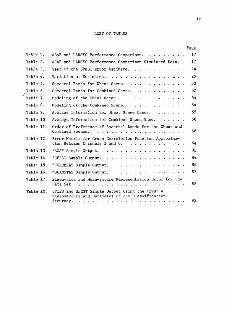

2
system according to defined conditions of optimality and (b) an ability
for convenient manipulation of candidate system parameters so as to
Permit comparison of the theoretically optimum designs with that of
practical approximations to it
In order to deal with the complexity of the design situation the
first step is to determine a suitable set of parameters which adequately
characterize it but is not so large as to be unmanageable It has been
observed [i] that there are five major categories of parameters which
are significant to the representation of information in remotely sensed
data They are
1 The spatial sampling scheme
2 The spectral sampling scheme
3 The signal-to-noise ratio
4 The ancillary data type and amount
5 The informational classes desired
Thus it is necessary to have present in the design machinery some means
for evaluating the impact of change in parameter values in each of these
five categories
Such a scanner design tool has been assembled in the form of a
software package for a general purpose computer Each of the parts of
this package called Unified Scanner Analysis Package (USAP) has been
carefully devised and the theory related to it fully documented [2 3 4 51
The goal of this report is to provide a documentation and description of
the software In constructing this documentation it was a~sumed that this
package will be useful for sometime into the future however it was also
assumed that it will only be used by a small number of highly knowledgeshy
able scientists
Section 2 recaps the theoretical concepts behind some of the primary
These are divi7ded into (a) scanner spatial charactershycomponents of USAP
istics modeling and noise effects (b) optimum spectral basis function
calculations (c) analytical classification accuracy predictions
3
(d) stratified posterior classification estimation and (e) an information
theory approach to band selection Although (e) is not a part of the
USAP system the results from this approach are helpful in understanding
the scanner design problem
Section 3 shows the integration of the above modules into the
software system Section 4 is the users guide to USAP describing the
required inputs and the available output products A listing of all
programs is provided in the appendix
The work which led to USAP was immediately preceded by a simulation
study of possible parametric values for the Thematic Mapper a new
scanner now being constructed for launch on Landsat-D in 1981 The
purpose of this simulation was to compare the performance for several
proposed sets of parameters We will conclude this introductory section
by briefly describing this work because it provides useful background
and serves well to illustrate the problem A more complete description
of this simulation study is contained in [l 6]
The general scheme used was to simulate the desired spaceborne
scanner parameter sets by linearly combining pixels and bands from (higher
resolution) airborne scanner data to form simulated pixels adding
noise as needed to simulate the desired SIN the data so constructed
was then classified using a Gaussian maximum likelihood classifier and
the performance measured The problem was viewed as a search of the
five dimensional parameter space defined above with the study localized
around the proposed Thematic Mapper parameters The scope of the
investigation was primarily limited to three parameters (a) spatial
resolution (b) noise level and (c) spectral bands Probability of
correct classification and per cent correct area proportion estimation
for each class were the performance criteria used The major conclusions
from the study are as follows
4
1 There was a very small but consistent increase in identification
accuracy as the IFOV was enlarged This is presumed to stem
primarily from the small increase in signal-to-noise ratio with
increasing IFOV Figure 1
2 There was a more significant decrease in the mensuration accuracy
as the IFOV was enlarged Figure 2
The noise parameter study proved somewhat inconclusive due to3
the greater amount of noise present in the original data than
desired For example viewing Figure 3 moving frolm right to
left it is seen that the classification performance continues
the amount of noise added is decreased until theto improve as
point is reached where the noise added approximately equals that
already initially present Thus it is difficult to say for
what signal-to-noise ratio a point of diminishing return would
have been reached had the initial noise not been present
4 The result of the spectral band classification studies may also
be clouded by the noise originally present in the data The
relative amount of that change in performance due to using
80-91 jimdifferent combinations of the 45-52 Jm 74-80 vtm
and 74-91 Pm bands is slight but there appears to be a slight
preference for the 45-52 jim band The performance improvement
of the Thematic Mapper channels over those approximating Landsat-l
and -2 is clear however
5 Using spectrometer data it was verified that the 74-80 vm and
80-91 Pm bands are highly correlated
6 Correlation studies also showed that the range from 10-13 Pm
is likely to be an important area in discriminating between earth
surface features Further it is noted that the absolute
calibration procedure described above results in a global
atmosphere correction of a linear type in that assuming a
uniform atmosphere over the test site the calibration
procedure permits a digital count number at the airborne
scanner output to be related directly to the present reflectance
of a scene element
The noise level in the original AC data was equivalent to about 005 NEAp
on the abscissa See Reference [ll
-----------------
5
10shy
-815 NDakota
Reflective Emissive IFOV Wm
Figure 1 Classification Performance vs Spatial Resolution
10 ---- 76 Kansas 0 815 U Dakota
0 30tO 40120 5012D 6012 80
ReflectiveEmrssive IFO( m) LANDSAT 2
Figure 2 RMS Error of Proportion Estimates vs Spatial Resolution
Nois Aded (EAPor4~c610c
geo
DL -Mshy7 0 or D2 D3 (x -0o6f
7
2 SCANNER PAPAMETERS ANALYSIS TECHNIQUES
Based upon the parametric approach introduced above the development
of a parametric scanner model must give explicit concern for the spatial
spectral and noise characteristics of the systems This is what has been
done in the Unified Scanner Analysis Package (USAP) shown in Figure 4
USA is composed of two distinct subsystems The spatial aspect of it
contains (a) a data spatial correlation analyzer (b) a scanner IFOV
model and (c) a random noise model The spectral techniques are capable
of producing an optimum spectral representation by modeling the scene as
a random process as a function of wavelengthfollowed by the determination
of optimum generalized spectral basis functions Conventional spectral
bands can also be generated Also studied was an information theory
approach using maximization of the mutual information between the reflected
and received (noisy) energy The effect of noise in the data can be
simulated in the spectral and spatial characteristics Two different data
bases are used in the system The spectral techniques require field
spectral data while the spatial techniques require MSS generated data
aircraft andor satellite The system performance defined in terms of
the classification accuracy is evaluated by two parametric algorithms
A detailed system description and users guide is presented in Sections 3
and 4 In the following the theoretical ideas behind the five major
elements of USAP are discussed
21 Analytical Classification Accuracy Prediction
Throughout the analysis of remotely sensed data the probability of
correct classification has ranked high among the set of performance indices
available to the analyst This is particularly true in a scanner system
modeling where generally the optimization of various system parameters
has as its prime objective the maximization of the classification accuracy
of various classes present in the data set
The estimation of the classification accuracy is fairly straightforshy
ward if Monte-Carlo type methods are employed In system simulation and
modeling however such approaches are generally a handicap due to their
Figure 4 Block Diagram of the Unified Scanner Analysis Package (USAP)
LARSYS CORELAT SCANSTAT
MSS Image Data Spatial Statistics statistics Noise Data Retrieval Correlation IFOlV Model
M(Satelliteod [or AC) In l zeA
A P~
SAnalytic
AClassification - Accuracy -Pc Predictor
Spectral Statistics
SPEST
Stratified Posterior A
Performance
Estimator
EXPSYS SPOPT SPTS
Opt Spect Data TransformationLab or DaIt Spectral Data Optimum
Field Retrieval Ensemble Sample Spectral Functions [ and
Band Function Statistics Ca eulationSpectral Thaid Data Construction - Calculation
Band
Specification
Implies path for spectralspatial statistics
Implies path for data or spectral functions
c
9
heavy dependence on an experimental data base the availability of which
can be limited due to a variety of reasons What is required therefore
is a parametric classification accuracy estimator for a multiclass
multidimensional Gaussian Bayes classifier This procedure should require
the class statistics mean vectors and covariance matrices as its only
input and produce a set of probabilities of correct classification
This technique has been developed tested implemented and comprehensively
reported [2] The following is a summary of the method and some results
The probability of Error as an N-Tuple Integral
The classification of a multidimensional observation vector into
one of M populations is conceptually identical to the binary case Let
0 M and N be the feature space number of classes and the dimensionality
of Q respectively The procedure is to divide 2 into M mutually disjoint
sets Pi and to assign each feature vector to a set in accordance with -
an appropriate rule This is illustrated in Figure 5 Let Zi i = 1
2 M partition S1in R The Bayes risk is defined as
R = i J P(m) Ci f-Xlw) dX 1~ Z J=l
I
is the cost of deciding w1 where w is true In the case where
C=0 for ij and C=1 for ij R is the probability of error iJ 1
where C 13 i1
Among all possible choices of Z the Bayes rule partitions Q into1
Z=Z such that R=R is the the minimum probability of error Assuming1 1
that the population statistics follows a multivariate normal law the
optimum Bayes rule is as follows [7]
X a W3 if W lt W Vi j - 1 2 M
where
Wi = (X- i)T [i-1 (X-_u + ln[iZ-21n P(o)m
i0
~wo2 ~~WM
Allocation of a Measurement Vector X to an Appropriate Partition
F-igure5 of the Feature Space
with
X = observation vector
= mean vector for class w (2)
= covariace matrix for class 1
P( i) = apriori probability for i
The error estimate based on direct evaluation of Eq (1)exhibits all the
desired-properties outlined previously
The evaluation of multiple integrals bears little resemblance to
their one dimensional counterparts mainly due to the vastly different
domains of integration Whereas there are three distinct regions in one
dimension finite singly infinite and double infinite in an N dimensional
space there can potentially be an infinite variation of domains The
established one dimensional integration techniques therefore do not
carry over to N dimensions in general Hence it is not surprising that
no systematic technique exists for the evaluation of multivariate integrals
except for the case of special integrands and domains [8] The major
complicating factor is the decision boundaries defined by Eq (2) P is
defined by a set of intersecting hyperquadratics Any attempt to solve
for the coordinates of intersection and their use as the integration limits
will be frustrated if not due to the cumbersome mathematics because of
impractically complicated results
In order to alleviate the need for the precise knowledge of boundary
locations and reduce the dimensionality of the integral a coordinate
transformation followed by a feature space sampling technique is adopted
The purpose of the initial orthogonal transformation of the coordinates
is an N to 1 dimensionality reduction such that the N-tuple integral is
reduced to a product of N one dimensional integrals Let the conditional
classification accuracy estimate Pc be the desired quantity Then
the transformed class w statistics is given by
12
j = 1 2 M (3)
-3-S = 0T 0
where 0 is the eigenvector matrix derived fromi Naturally in each
transformed space Ti(Q) wi has a null mean vector and a diagonal
covariance matrix
The discrete feature space approach is capable of eliminating the
If 0 is theneed for the simultaneous solution of M quadratic forms
continuous probability space a transformation Ti is required such that
can be completely described in a nonparametric form therebyin TiQ) r1 1
bypassing the requirement foran algebraic representation of P This
desired transformation would sample Q into a grid of N-dimensional
hypercubes Since the multispectral data is generally modeled by a
multivariate normal random process a discrete equivalent of normal
random variables that would exhibit desirable limiting propertiesis
Let ynBi (n p) be a binomial random variable with parametersrequired
n and p The x defined by
Yu- npx Yn 0i 2 n (4)
converges to xN(O 1) in distribution [91 ie
lim F (X) - - F(x)n
The convergence is most rapid for p= then
(yn - n2)2 (5)n
13
The variance of xn is set equal to the eigenvalueof the transformed Yi by incorporating a multiplicative factor in Eq (5)
The segmentation of b a union of elementary hypercubes makes
nonparametric representation of P and its contours feasible Following1
the orthonormal transformation on o and sampling of 2 accordingly each1
cells coordinate is assigned to an appropriate partition of r This
process is carried outexhaustively therefore FI can be defined as a set
such that
r = ux x eli (6)
once the exhaustive process of assignment is completed the integral of
f(Xjwi) over Fi is represented by the sum of hypervolumes over the
elementary cells within P The elementary unit of probability is given by1
61 62 6N
f f (Xi) = 2 f (xli i ) dN T f (x 2 lo i ) d 2 2--2 f (xNIwi) dN
C -61 62 -N
2 2 2 (7)
where C is the domain of a sampling cell centered at the origin and 6
is the width of a cell along the ith feature axis The conditional
probability of correct classification is therefore given by
c Il+ 61 c2+ 62
Pcli - T (x i (x-l2) (C)dx2J f jw) (C)dx x c -6 2c -61
2 2
(8)
c +6 n n
c 2-- f (xNIwplusmn) II(C) dxN
c -6 n n
2
with overall classification accuracy given by
14
M
p P(m) P 1W (9)bullC I
where
1 if Cc (10)ii(C) =
0 otherwise
C = The domain of an elementary cell
Figure 6 is a geometrical representation of Eq (8)
Experimental Results
The analytic classification accuracy prediction (ACAP) has been
Two examples are repeated hepethoroughly tested and documented [2]
The first experiment investigates the performance of the estimator vs
Small to moderate range ofgrid size ie number of cells per axis n
Figure 7 n is required if computation time is to remain realistic
vs n for three classes having some hypotheshyshows the variation of Pcjw c1
The main property of the estimator istical statistics in 3 dimensions
its rapid convergence toward a steady state value thereby alleviating
the need for excessively fine grids and hence high computation costs
The data collected over Graham County Kansas is used to perform
a comparison between the ACAP algorithm and a ratio estimator such as
LARSYS The results are tabulated in Table 1
ff(x)
f(x~lQl)
xl
Figure 6 A Concentual
Illustration of the ACAP Error Estimation
Technicxue Using
Two Features FIEU
100C L A 1- CLASS I s -- 2- CLASS 2S
3- CLASS 51 r 110 0- OVERALL I CA as T I A
C 7S
C
PC
T So CHERNOFF BOUND- 447
ss tI1II
4 8 10 12 14S 7 9 11 15
NO OF CELLS PER RXIS
Figure 7 ACAP Classification Accuracy Estimate vs Grid Size for the Test Population Data 9
17
Table 1 ACAP and LARSYS Performance Comparison
Class No of Points LARSYS ACAP
Bare Soil 443 659 783
CornSorghum 99 899 910
Pasture 1376 984 950
Wheat 459 948 939
Overall 2377 872 896
The comparison of ACAP and LARSYS results from Table 1 is inconclusive
In some cases the difference is negligible (corn) and in some significant
(bare soil) Examination of the data statistics revealed that the
assumption of normality does not hold throughout the populations statistics
This problem can be rectified by simulating random Gaussian data having
identical statistics with the real data hence assuring the normality
assumption Repeating the LARSYS and ACAP procedures produces a new set
of classification accuracies Table 2
Table 2 ACAP and LARSYS Performance Comparison Simulated Data
Class LARSYS ACAP Accuracy Difference
Bare Soil 778 783 05
Corn 912 910 - 02
Pasture 953 951 02
Wheat 942 939 02
Overall 896 896 0
The differential between ACAP and LARSYS results has been narrowed
considerably ranging from a high of 05 for bare soil to 0 for the
overall classification accuracy Two conclusions can be drawn from the
results of this experiment First the ACAP and Monte Carlo type
classifiers produce practically identical results if the underlying
assumptions are satisfied (eg normality of the statistics) Second
and more revealing is the fact that the results of the ACAP processor
indicated an upper bound for the classifability of bare soil had
18
its statistics been Gaussian This result is a direct property of ACAPs
data independence Figure 8 is the ACAP estimator vs n for Graham Co
data
The above selected experiments and others reported in the biblioshy
graphy establishes ACAP as a viable and necessary tool in any analytical
remote sensing data collection system modeling and simulation when the
performance index is defined as the probability of correct classification
22 Stratified Posterior Classification Performance Estimator
The second classification accuracy estimator to be presented here
(SPEST) is based on the maximization of the aposteriori probability
associated with each sample This formulation is closely related to
the maximum likelihood principle used in the ACAP The distinction
arises in the determination of integration domains Where in ACAP a
deterministic grid was set up to sample the feature space SPEST uses
an internally generated random data base and assigns the feature vector
to the appropriate class via the maximum aposteriori principle Due to
the different approaches adopted the statistical properties of the
estimators could be substantially different although no major study has
yet been carried out It has been observed however that the SPEST
algorithm is somewhat faster than the ACAP in selected cases The
approach here is similar to that described in Moore Whitsitt and
Landgrebe [10]
1 2 3 MLet X be an observation from one of M classes wi i =
with a priori probabilities P The maximum likelihood decision rule can 1
be stated as follows Assign X to the class w k if
P(ikIX) = max P(wiX)JX) i
This rule partitions the observation space Q into subregions FI 12 PM
corresponding to the classes il ()2 M respectively Define the
indicator function as
C 100-U
A
4 - - - 4 - - 4 - 4 - -- 4 - - -S4 ~_ ---- 4- --- -4
FI ~~~
N 4
R C I- CLASS 1 C 2- CLASS 25- CLRSS 5 R 4- CLASS 4 C 0- OVERRLL Y
PSC
T ) 1
7S I I 4 8 10 12 14 16
s 7 9 11 15 15 17
NO Or CELLS PER RXIS
Figure 8 ACAF Classification Accuracy Estimate vs Grid Size for Graham Co Kansas Data
kH
20
The probability of correct classification integral is given by
Pc = f M I(x) p(xi) dx (11)
It is desirable to evaluate the probability of correct classification for I
each class as well as the overall probability The performance probability
for the ith class is
Pci = JI i(x) p(xltamp (12)
The overall performance then is
M
p = iPci (13) c i= l1 c
From Bayes rule
P(mijx) p(x)
p(xli) P
hence
Pci = l(x) ptn p(x) dx
p(x) is a mixture density
M
p(x) = X P pjx jl p (
21
Therefore
M P
I - T2 x) P(4)Ix) p(xV1 ) dx (14)Pc1 j=l P i (
Define
Qi(x) = Ii(x) P((i Ix)
Then
f Qi(x) p(xIW) dx
is the conditional expected value of Qi(x) given that X comes from the
class C The estimate
M p N
(15)j=l PN I Qi(xk)j=P5 jJ k=l
is unbiased This estimator is similar to the stratified posterior
estimator described by Whitsitt [10]
To do this a pseudo-random sequence of uniformly distributed random
digits is generated by the power-residue method and is transformed by the
inverse cumulative-distribution-function method to obtain nearly Gaussian
samples These samples are used to fill the elements of the data vector Y
Each vector Y then has expected value 0 and covariance matrix I
By performing the transformation
X = F Y + m (16)J j - -3
22
On the vectors I the random vectors for class j are obtained where 4
is the matrix of eigenvectors required to diagonalize the covariance matrix
of class j rS is the diagonal matrix of eigenvalues and m is the desiredJ
These random vectors are used to evaluate the estimators in mean vector
Eqs (15) and (13)
The term that must be evaluated from Eq (14) is
P p(xlwo)
P(CIx) = YPk P(X_ k Q
k
To evaluate this probability compute P p(xloj) for each class w Choose
the largest value of the product P p(xlm) and divide by the sum P P(XLk)j k
P(x~mk) = exp - (x-mk)T K1 (x - m) (17)
(27F) 2K I
and Kk are the mean vector and covariance matrix respectively for class
k Substituting Eq (16) into (17)
p(xIk) = - exp - T T- Y
2YT r T -1 1 -18 -2 -j Kk (-m-mk) 4 (m-mk) K (m-mk)] (18)
In this form it is not necessary to perform the intermediate computational
step of transforming the data We need only to generate M sets of random
vectors Y with mean vector 0 and covariance matrix I and use them in the
Eq (18)
23
Estimator Evaluation
A subroutine program was written to evaluate classification perforshy
mance by the above method To test the method a three class problem was
constructed The mean vectors for the classes were
1 ]T
S = [-i -i ]T M 2 [0 0
N2 T L3 = [ ]
The covariance for each class was the identity matrix The number of
random vectors generated for each class was 1000 The exact classificashy
tion accuracy as a functidn of the dimensionality can be evaluated for
this case
P = 1 - erfc (fi2)
Pc2 = 1 - 2 erfc (VN2)
P = 1 - erfc (A-2)
P =1 - 43 erfc (AT2)c
t~ -X22
where erfc (a) = edx
and n is the number of dimensions Table 3 contains the results of
evaluating the class conditional performance and overall performance
from one to ten dimensions
To evaluate the variance of the estimates different starting values
for the random number generator were used Twenty trials were used to
evaluate the maximum bound and the standard deviation from the true value
These results are presented in Table 4
For the overall accuracy the estimate is within 005 of the true
value This is certainly sufficient for performance estimation The
Table 3 Test of the SPEST Error Estimatd
Pc1c P P P Pc2 Pc30
1 06915 03829 06q15 05886 06859 03793 07001 05884 2 07602 05205 07602 06803 07671 05116 07700 06829 3 08068 0613j5 08068 07423 08037 06202 08081 07440 4 084-13 06827 08413 07885 08283 06852 08550 07895 5 08682 0-7364 08682 08243 08642 07425 08703 08256 6 08897 07793 08897 08529 08767 07939 08787 08498 7 09071 0814I 0907i 08761 08993 08242 09065 08766 8 09214 08427 09214 08951 09129 08472 09240 08947 9 09332 68664 09332 09109 09193 08809 09360 09120
10 09431 08862 6943i 0924i 09209 09012 09481 09234
25
Table 4 Variation of Estimates
pcl Pc2 Pc3 Pc
1 016 010 017 003 a 033 019 049 005 Bound
2 018 010 014 002 a 036 018 027 005 Bound
3 016 017 017 003 C
046 031 055 007 Bound
4 011 016 015 003 a 025 029 029 005 Bound
5 015 014 012 002 a 031 033 026 004 Bound
6 014 014 010 003 a 026 023 022 006 Bound
7 009 016 012 003 a 027 033 027 005 Bound
8 013 013 012 003 025 036 023 006 Bound
9 013 014 012 002 a 026 031 021 004 Bound
I0 009 012 009 002 a 016 024 019 005 Bound
a = standard deviation
Bound = maximum difference between estimate and true value over 20 trials
26
class conditional estimates are less reliable but are sufficient to
observe trend in the performance due to individual classes
23 Scanner Spatial Characteristics Modeling
The multispectral scanner represents themost important element in
a remote sensing data gathering system Therefote an understanding of
the signal flow through this subsystem is essential As data is processed
through the scanner its statistical properties undergo a transformation
This in turn will alter the population separabilities and hence the
classification accuracies The comparison of this quantity at the scanner
input and output and observationof its variation with the system parashy
meters sheds considerable light on the overall system design Since the
Bayes Ppectral classifier depends solely on the population of spectral
statistics methods need to be developed that relate the scanners input and
output statistics A complete derivation of such relationship is given
in Appendix A of [2] A summary follows
Scanner Characteristic Function
Figure 9 is a basic block diagram of the scanner spatial model where
f through fN are N stochastic processes corresponding to N spectral
bands and h(xy) is a two dimensional PSF In particular where the Landsat
scanner is concerned the assumption of a Gaussian shaped IFOV has been
widespread Let f(xy) g(xy) and h(xy) denote the input and output
random processes associated with any two matching bands and the scanner
PSF respectively It is well known that the above quantitfes are related
by a convolution integral
Jg(xy) f f(x-1y-A 2 ) h(XV1 2) d IdX 2 (19)shy
it follows that
S(UV) SIf(uv)IH(uv)l2 (20)
27
n(xy)
f2 h(xy)+ 92
f- _-+ gN
Figure 9 Scanner Spatial Model as a Linear System
28
where S(uv) is the spectral density of the appropriate random process
and H(uv) is the two dimensional Fourier transform of the scanner PSF
Let M(uv) = IH(uv)12 afd m(Tn) its inverse transform Then the output
spatial autocorrelation function is given by
R (Tn) = Rff(Tn) m(Tn) (21)
In order to obtain specific results the following assumptions are
invoked (a) exponential data spatial correlation (b) Gaussian IFOV
PIT I Rff(Tn) = 011 rn 0 1 2
(22)
2 2 h(xy) = c1 e - e2
r r 0 0
=-a =-b where px = e and py = e are the adjacent sample and line correlation
coefficients respectively r is the scanner PSF characteristic length
O in-pixels and c1 a constant providing unity filter gain Using the
separability property of the functions inv6lvedi
R g(TI) = Rff(T-X-) m(x) dx f Rff((Th-y) rn(y) dyJ where
c 2 2 r0 2 2 n
m(rr) = 2 e 2r 2e 2- 2 (23)
0 0
carrying out the integration the scanner characteristics funation is
given by
29
2 a222 lar a r
_- -aT +a
W (TIab) = Q(ar --L-) + e Q(ar +U)X 0 0
bt~rr 2or Qb l
o + o +bf
2Lr- Q(br2Q(br ) (24)e
where
2x
Q(x) = e 2
The spectral statistics is a subset of the spatial statistics hence
W (00ab) defines the ratio of the variance at the scanner output to s
the corresponding input quantity
The output crosscovariance terms can be similarly derived Let
the crosscorrelation function between bands i and j be defined as
Rff (T) = rffaf of e-aeIrI -biiI (25)213 1J 1 j
where rf f is the spectral crosscorrelation-coefficient at the input
such that Irff I lt 1 aij and bIj are defined similar to a and b with
the additional channel specification Following the previous technique
it follows that the crosscovariance term between channels i and j is
given by
Rggj (00) = rffoff off Ws(00aijb)ij (26)
1J 1 J i i ij 12 2
30
The corresponding crosscorelation coefficient follows
W (00a ibi) Sgigj - rff
w 2(00aii~bii) WbOOa b) i s si 33 33
Therefore the band-to-band correlation coefficients are identical at
input and output provided the spatial auto and crosscorrelashythe scanner
tion function at the input are equivalent ie aiiaij biib ij A
closed expression can also be obtained for a rectangular PSF defined by
I~o Ix lyl o2
(28)h(xy) =
0 elsewhere
the corresponding characteristic function is given by
-a r
(i1 - ) X -lW (OOa)= 2 l-e 110
s O aiii ar ar I 0 11 0
-br
br2 (I l-er 110 -) (29)
ii o ii 0
Eq (24) and Eq (29) are plotted in Figures10 through 13 for different
as a running parameter The scene correlations with the IFOV = r0
of either PSF is the increasing outputuniversal property exhibited by Ws
variance reduction as IFOV is increased This property hasbeen widely
verified experimentally Comparison of Figumsll and 13 indicates that
for the same IFOV a Gaussian shaped IFOV causes a heavier variance
a rectangular PSFreduction in a spectral band than that of This
property can potentially produce a higher separability among the populashy
tions as the signal is processed through the scanner electronics
W 1 GAUSSIAN SCANNER PSF EI
H INCREASING IFOV (i PIXELSTEP)T 8
I N G7
F A C T0 R
2 2 N 8
0 1 is 2 6 5 5 5 4 5 s S 5 e 7 5 a s 96 95
ADJACENT SAMPLE CORRELATION
Figure 10 Scanner Characteristic Function vs Scene Correlation Adjacent Line Correlation = 65
W GOUSSIRN SCANNER PGF E I G H
N
T 8INCREASING IFOV (I PIXELSTEFP
C
R
FA
T0
04
1 15
2
2s
5S
4 8 4S 5 75
ROJPCENT SRMPE CORRELATION
8 85 S
Figure 11 Scanner Characteristic Function vs Scene Correlation Adjacent Line Correlation = 8
E 1 GRUSSIRN SCANNER PSF
H T8 I N G F A
INCREASING IFOV (1 PIXELSTEP)
T
R
4
2
1
1
15
2
25
5s
4 S 7
4S 55 8s 7S
ADJACENT SRMPLE CORRELATION
85
9 95
Figure 12 Scanner Characteristic Function vs Scene Correlation Adjacent Line Correlation = 1
1 RECTANGULAR SCNNER PSF
I 9 rINCREASINGH IFOV (I PIXELSTEP)
T I N G
F A C T 0
4
2
IA 2 4 68 7 8 1s 2S 5s 4S SS s 7S 85 9s
ADJACENT SANPLE QORRELATION
Figure 13 Scanner Characteristic Function vs Scene Correlation
Adjacent Line Correlation = 8
35
The input-output statistical relationship just developed along with
the analytic classification accuracy predictorprovide the two basic
tools required for a parametric evaluation of the MSS performance under
varying operating conditions As an illustration three hypothetical
classes with some prescribed statistics are specified at the scanner
input Three different sceneswith adjacent sample correlations of 05
085 and 095 are considered The scanner characteristic function
produced a set of transformed statistics at the output followed by the
estimation of the conditional classification accuracies using ACAP for
8 different IFOVs The results are plotted in Figuresl4 through 16
Two main properties stand out First is the improvement in class
separability as the IFOV is enlarged This is true in all the cases
The rate of improvement however is strongly correlated with the scene
spatial correlation The lower the input scene correlation the higher
the classification accuracy improvement per IFOV step This property
is brought about by the characteristics of Ws where one step increase
in IFOV size produces a greater variance reduction for a low scene
spatial correlation than a similar increase would cause in a highly
correlated scene
The scene spatial correlation plays a significant role in the overall
system performance which is not readily obvious One of the well
known properties of linear systems with random inputs is the reduction
of the output varianceinput variance ratio as the point spread function
(PSF) is widened In this section it has been shown theoretically that a
third factor in this reduction is the spatial correlation structure of
the input stochastic process Specifically with everything else fixed
a process having a moderate scene correlation will undergo a tighter
clustering around its mean than an otherwise identical process with a
highly correlated spatial characteristic On the extreme side of the
correlation scale with a small pixel-to-pixel correlation the ratio of
the output variance to the corresponding input quantity is very negligible
Consider a bandlimited white noise process with a spectral density
shown in Figure 17where W is the bandwidth and No2 the two sided specshy
0 1001
I go
C Rq T S86
N
P8r C C U 7 153 R R C Yr 70
1
I1- CLSSS
2- CLRSS
I
C T 85
3-0-
CLRSS 5 OVERRUL
SCFRNNER IFOV IN HIGH RESSLUTION PIXELS
Figure 14 Scanner Output Classification Accuracy vs Ifl Adiacent Sample Correlation = 55w
C 100
L R S I F
Ao
T1 85
0 N
8 0f1C C U 75 R C I- CLASS I Y 70
2- CLASS 2 F 3- CLASS 5C
0- OVEWILLT BE
742
SCANNER IFOV IN HICH RESOLUTION PIXELS
7Figure 15 Scanner Output Classification Accuracy vs IFONAdjacent Sample Correlation = 8
10c LAS 9- O SI F
CC 2- CLASS 2
1 85 T 3- CLA~SS 5 0 0- OVERALL
N
A80 C
UR
C 7S
C Y 70
P
T GS
2 4 8
SCRNNER IFOV IN HIGH-RESCUTION PIXELS
Figure 16 Scanner Output Classification Accuracy vs IFOV Adjacent Sample Correlation = 95
00
39
No2
-2gW 27W w
Figure 17 Bandlimited White Noise Spectral Density
tral density As W increases the adjacent pixel correlation in the
scene decreases The increase in W however is accompanied by a
decrease in No2 if this process is to remain physically realizable
(finite energy) Under a finite energy constraint therefore as W-shy
No2-- 0 In the limit the energy content of the output random process
will be nil
Random Noise
Additive random noise entered at various stages of a scanner system
can degrade the overall system performance substantially The noise can
be classified into two broad categories external and internal A
major source of external noise is atmospheric in nature mainly due to
absorption (eg water vapor) and scattering The detector and quantishy
zation noise comprise the major component of the internal noise sources
From a system analysis point of view the latter represents a more tractshy
able and better understood component of the random noise [11] while
the former still awaits further experimental documentation The purpose
of this work is not so much the exploration of the various noise sources
but the integration of its effect within an analytic analysis package
once its characteristics and origin has been determined
can be stated that atmosphericFrom the theoretical results obtained it
noise in the uplink path at least has negligible degrading factor
compared with the detector and quantization noise Let f(xy) Nf(xy)
f(xy) and Nf(xy) be the input random process input additive white
40
noise the output random process and the noise component of the output
signal respectively then
f-(xy) = f(xy) h(xy) (30)
N (xy) = Nf(xy) h(xy) (31)f
Define
(SNR)f = Var f(xy)1Var Nf(xy)l (32)
(SNR) -= Var f(xy)Var N (xy)) (33) f f
Recalling the functional dependence of Ws on the input scene spatial
correlation it follows that the ratio of the variance of a white noise
process at the scanner output to the corresponding input quantity is of
the order of 5 to 10 higher or lower depending on the IFOV size
Therefore
Var f(xy) lt Var f(xy)l (34)
Var N (xy)l ltlt Var Nf(XY (35)f
hence
(SNR) f gtgt (SNR)f (36) f
It then follows that the noise component of the output process prior to
casesdetector and quantization noise is negligible in most
In order to observe the effect of noise on the scanner output class
separability the test class statistics were modified to exhibit the effect
of random noise The assumed properties of the noise are additive
white and Gaussian Let F-(xy) )e the signal to be teJmeterud to
Earth
41
f(xy) = f(xy) + N (xy) (37) f
the statistics of f(xy) and f(xy) are related by
+ Y (38) r~f -N
f
the simple addition is due to the signal and noise independence Assuming
a zero mean N the mean vector are identical ie f
E ffj = E f-)
Among the four assumptions about the noiseits Gaussian property is the
weak link due to the Poisson distributed detector noise and uniformly
distributed quantization noise Relaxing the Gaussian noise assumption
however would mean the design of an optimum classifier for non-normal
classes and evaluation of its performance A task that would complicate
matters considerably Due to the relatively insufficient documentation
of the characteristics of random noise in multispectral data the initial
Gaussian assumption is adhered to
Following the adopted SNR definition three different noise levels
are considered and the corresponding overall classification accuracies
for the three previously used test classes are estimated Figure 18 is
the variation of P vs IFOV with SNR as the running parameter For a c
fixed IFOV P increases with increasing SNR For a fixed SNR P c c
increases with increasing IFOV size These illustrations have shown
that with a proper coupling between the ACAP and the scanner characteristic
function the progress of the population statistics through the system
can be studied on an analytical and entirely parametric basis The
accompanying classification accuracies can measure the designers success
in selecting the spatial andor spectral characteristics of a Multispectral
Scanner System
C S LSs
1 80 SNR-50 0BF 8 I C R
I 7 -0 N
T
37cent0 U
C
R
C Y ( 6s-- SNR=10 0B P 6 C T
2 4 6
SCANNER IFOV IN HIGH RESOLUTION PIXELS
Figure 18 Overall Output Classification Accuracy Variation with Noise and IFOV
43
24 Optimum Spectral Function Research
In earth observational remote sensing much work has been done with
extracting information from the spectral variations in the electromagnetic
energy incident on the sensor Of primary importance for a multispectral
sensor design is the specification of the spectral channels which sample
the electromagnetic spectrum An analytical technique is developed for
designing a sensor which will be optimum for any well-defined remote
sensing problem and against which candidate sensor systems may be compared
Let the surface of the earth at a given time be divided in strata
where each stratum is defined to be the largest region which can be
classified by a single training of the classifier Each point in the
stratum is mapped into a spectral response function X(X) as in Figure 19
That is if one observes a point in the stratum with the sensor then the
function X(A) describes the response variations with respect to the
wavelength X The stratum together with its probabilistic description
defines a random process and the collection of all of such functions
X(X) which may occur in the stratum is called an ensemble
The general concept of a pattern recognition system in this applicashy
tion requires that if each X(X) is to be classified by a classification
algorithm this can be accomplished by first measuring a finite number
of attributes of X(A) called features This is the function of the
sensor system as depicted in the upper left portion of Figure 20 where
X1 X2 X are the values of N features for a given X(X) It
may be viewed as a filtering operation on X(A)
For example on the right portion of Figure 20 the function of MSS
of the Landsat satellites is illustrated In this case a number proporshy
tional to the average energy in a wavelength interval is reported out by
the sensor for each of four wavelengths Mathematically this may be
expressed as
Zn f X n)(X)dX n = 1 2 3 4
44
Next we must consider what would constitute an optimum sensor We
first note that in general the sensor may be used over any part of the
earthb surface at anytime and for many different applications (sets
of classes) Therefore the sensor must be optimized with respect to the
entire set of strata represented by these cases As a result of the large
size of this set and the fact that its statistical description is not
known we will optimize the sensor with respampct to its signal representashy
tion characteristics The fX(A) each contain information Useful to the
classifier we require of the sensor design that for a given N a maximum
of this information which was in X(A) still be present in X Since n the specific nature of this information is not known a priori we can
only assure that this will be the case for any stratum if X(A) is
recoverable from fX I n
Let X(A) be the result of attempting to reconstruct X(A) from X n
A fidelity criterion which is useful in this instance is
= f[X(X) - x(X)] 2 dA (39)
the so called mean square error or mean square difference between X(X)
and X(A)
It is known [12J thata reconstruction scheme which minimizes C for
a given N is
X(A) = XI1 (A) + X2 2(A)+ + +n(A)
N X + (A) (40)
n=l
provided that the n(A) are orthogonal over the wavelength interval of
interest ie
S m(X)n(X) d) = 0 m n (41)
Stratum The Ensemble
A
A
A
Figure 19 Realization of a Stratum as the Ensemble of Spectral Sample Functions
Figure 20 Basis Function Expansion of a Random Process
x(AxSensorI X2
XN
A A
I
I
I
I-- i
X1lA) =Xl~il l +X2I2A]I+
4SNA)
^
47
and the X are calculated byn
X = X(x) Mn(3dA (42)
Note for example thatthe Landsat example of Figure 20 satisfies
these conditions In the lower right of Figure 20 is depicted the
result of such a reconstruction for the Landsat example
While use of Eq (42) in the case does minimize s with respect to
the choice of values of TX 1 a further improvement may by obtained byn
choosing a set of iIXI which minimizes E Itcan be shown [5 12]
that the set n(X) which accomplishes this must satisfy the equation
U = R(AC) C()dC (43)
where
R(XC) = E[X(A) - m()] [X( ) - m( )]1 (44)
is the correlation function of the random process and m(X) is its mean
value at X
Such a signal tepresentation defined by Eqs (40-44) is known as a
Karhunen-Lo~ve expansion [13] It provides not only for the most rapid
convergence of X(X) to X(X) with respect to N but in addition the random
variables (X are uncorrelated and since the random process is Gaussian n
they are statistically independent Further the only statistic required
of the ensemble is R(XC) This representation of X(X) is therefore
not only optimal it is convenient
A useful generalization of the Karhunen-Lo~ve expansion can be made
Suppose a priori information concerning portions of the spectral interval
are known and it is desired to incorporate-this knowledge into the analysis
A weighting function w(A) is introduced which weights portions of the
interval according to the a priori information As an example measureshy
48
ments were taken over the spectrum and it was observed that there was
considerable variation in the signal in the water absorption bands
around 14 and 18 micrometers This variation was due to measurement
and calibration difficulties rather than being a result of variations
in the scene Therefore the weighting function was set to zero in
these absorption bands This generalization is referred to as the
weighted Karhunen-Lo~ve expansion [5] Eqs (40) (42) and (43) become
N X(A) = x( AsA (45)
i=1l
a (A) = FR(AE) w( ) 4 (E)dE (46)w i f w
x X(A) w() tw (X) dA (47) 1
where the eigenfunction 41 (A) are solutions to the integral Eq (46)W 1
with the weight w(A) The special case where w(A) = 10 for all AcA
reduces the expansion to the original form in Eq (40) (42) (43) and
(44)
The results of having utilized this means of optimal basis function
scheme on spectral data are contained in reference [5] From them one car
see the significant improvement in classification accuracy which decreased
spectral representation error will provide One can also determine the
spectral resolution and band placement needed to achieve such classification
accuracy improvement
25 Information Theory Approach to Band Selection
The ptoblem of selecting a set of optimum windows in the electroshy
magnetic spectrum for observing the reflected sunlight has always been of
considerable interest Depending on the definition of the optimality
different methods have been developed One such approach was shown in
Section 24 using K-L expansion to select an optimum set of basis functions
In this section an information theoretic definition of optimality developed
in [3] is explored
49
Mutual Information and Stochastic Modeling
The reflected energy from the target is detected by the scanner
and corrupted by various noise sources If S is the noise-free signal
Y the observation and N a random disturbance then
Y = S + N (48)
the reduction of uncertainty about S obtained from Y is called the
average or mutual information between the observation and original signal
Since the reconstruction of the reflected signal from the noisy observashy
tion is the highly desirable capability the comparison of such average
information-and selection of these bands with the highest information
content is chosen as-a means of spectral band selection Let
S = (sl s 2 )
and
)Yn =(Yl Y2 Yn
where si and yi are the coefficients of the orthonormal (K-L) expansion
of Y and S then the mutual information between Y and S is given by [3]
T(YS) = - log et (49)
where C and C are the covariance matrices of (yi i = 1 2 ) and
(ni = No2 i = 1 2 ) and No2 is the two sided spectral density of
the additive white noise Equivalently I(YS) can be represented in
terms of the Wiener-Hopf optimum filter impulse response
A-(2
T()= J h(AA) dA (50)
11
50
h(XA) provides an estimate of S from Y with a minimum mean-square error
This relationship however is not a practic d-dethod of evaluating I(YS)
since the actual solution of the Wiener-Hopf integral itself is a nontriyal
task This problem can be circumvented by a discrete state variable
formulation ieshy
s(k+l) = _s(k) + FW(k) ke[Al x2 ] (51)
where
s1(k+l)
s2(k+l)
s(k+l) =
Sn(k+l)
is an (nxn) matrix
r is an (nxl) vector
W(k) = a descrete independent Gaussian
zero mean random process
The formulation of the problem in the discrete domain -provides a practical
way of computing hXX) through Kalman filtering techniques The discrete
version of Eq (50) is given by
I(YS) = - h(kk)
k 6 AA 2 (52)
The discrete nature of this approach makes the evaluation of Eq (52)
considerably more practical than its continuous counterpart This is due
to the fact that the Wiener-Hopf equation is easily solved in only those
cases for which the analytical form of Ks (Au) the signal eovariance
fnnction is fairly simple not likely for most-random processes encountered
51
in remote sensing Since h(kk) is dependent on the parameters of Eq (51)
a concise representation of s(k+l) is needed
The general form of Eq (51) is given as an autoregressive (AR)
model
m1 m2
s(k) = X as(k-j) + I bji(k-j) + W(k) (53) j=l J j1
s(k) = The spectral response at the discrete
wavelength k It is a Gaussian random process
w(k) = zero mean independent Gaussian disturbance
with variance p
(kj) = deterministic trend term used to account for certain characteristics of the empirical data
ab = are unknown constant coefficients to be I i determined
mlm2 = The order of the AR model
The identification selection and validation of general AR models
for the representation of a random process is a well developed technique
[1415] The identification of an appropriate model provides the
necessary parameters required for the evaluation of I(YS) in Eq (52)
The model selection process for a selected number of ground covers has
been carried out [3] leading to the ranking of a set of spectral bands
according to the criterion outlined previously A summary of the
experimental results are given below
Data Base and Model Selection
Two different sets of empirical data are used to demonstrate the
techniques developed here The first set consists of observations of
wheat scenes The second set consists of several vegetation cover
types such as oats barley grass etc For each scene the spectral
responses collected by the Exotech 20C field spectroradiometer are
averaged over the ensemble It is thought the resultant average
52
zspectral response provides a relatively good data set for demonstration
-purposes Figures2l and 22 show the average response for both cover
types
In order that the study be carried out in a context that is relashy
tively realistic for multispectral scanners the spectral response -of
the two data sets is divided into a cnumber -of spectral banids The division
is fairly arbit-rary but each band must contain a sufficient number of
data points to ensure accurate parameter estimation for model identifishy
cation The spectrum is divided into 9 bands from 045 pm to 238 pm
with two gaps in the 134-145 pm and 182-196 -pm range -due to atmosshy
pheric absorption see Tables 5 and 6
Table 5 Spectral Bands for Wheat Scene
Band Number Spectral Wavelength Interval (Pm)
1 045-054
2 054-062
3 062-071
4 071-085
5 085-099
6 099-013
7 113-134
8 145-182
9 196-238
Table 6 Spectral Bands for Combined Scene
Band Number Spectral -Wavelength Interval (pm)
1 045-054
2 054-062
3 062-071
4 071-085
5 -085-098
6 098-112
7 112-130
8 145-18 2
9 196-238
53
s15
10-
S
AX(Uir)0 0 1 2 2S
Figure 21 Average Spectral Response -- Wheat Scene
1I X im)
S
0
0 1 5 FS Rsp2s
Figure 22 Average Spectral Response -- Combined Scene
54
The next step is the identification and validation of models that
would adequately describe the aforementioned spectral responses Three
different models were tested and compared (a) autoregressive (AR)
(b) autoregressive plus a constant trend (AR+C) (c) integrated
autoregressive (I-AR) Following the standard selection and validation
techniques one of the above 3models is selected which describes the
scene most satisfactorily Tables7 and 8 show the selected models for
the wheat and combined scene respectively IAR-2 in Table 8 in a second
order IAR
Table 7 Modeling of the Wheat Sc~ne
Band Order of Model
1 7
2 2
3 11
4 1
5 1
6 2
7 5
8 8
9 6
Type of Model
AR
AR
IAR
AR+C
AR
AR+C
IAR
IAR
IAR
Table 8 Modeling of the Combined-Scene
and Order of Model Type of Model
1 11 IAR-2
2 2 AR
3 11 IAR
4 1 AR+C
5 3 AR
6 1 AR
7 9 AR+C
8 8 tAR
9 1 AR
55
Spectral Band Selection
It was initially stated that the information content of a set of
spectral bands can be used in the selection of an optimum subset Here
the preceding regression analysis will be used to evaluate the mutual
information between the reflected energy and the observed signal in the
9 spectral bands under study
The first step is the computation of the average information in y(k)
the received spectral process about s(k) The reflected spectral scene
response as a function of spectral bandwidth for each band of both
scene types The average information is computed for several values of 2
the noise variance a N Appropriate software is developed to carry out
the calculation of I(YS) Figures23 and 24 show the variation of
I(YS) in nats for the wheat and combined scene in band 1 Similar plots 2 -3are shown for the infrared band 7 Figures 25 and 26 Selecting a a = 10
for demonstration purposes the average information for wheat and combined
scenes are tabulated in Tables9 and 10 for 9 spectral bands
Table 9 Average Information for Wheat Scene I
Band I(YS) nats
1 3450
2 1052
3 2035
4 3000
5 4496
6 3720
7 6031
8 3480
9 5010
56
0
-51080 I(nats)
40--1shy
20shy
a -Io
k 1
1080400
Figure 23 Average Information Band 1 Wheat Scene
s I(nats) 10-5
10
0 40 0 120
20 40 L00
Figure 24 Average Information Band 1 Combined Scene
57
10 - I (nats)
10-5
7510
so
2s 10shy2
o = i0-1 26
n
0 - k 0 100 200
so ISO
Figure 25 Average Information Band 7 Wheat Scene
100 1(nats)
7S 7-5 10 3
0-2
100 200 s0 IS0
Figure 26 Average Information Band 7 Combined Scene
0
58
Table 10 Average Information for Combined Scene Band
Band I(YS) nats
1 4133
2 1617
3 2298
4 4008
5 4573
6 4096
7 7825
8 6415
9 7419
Using the information content of each band as an optimality criterion
the 9 spectral bands can be ranked see Table 11
Table 11 Order of Preference of Spectral Bands for the
Wheat and Combined Scenes
Rank Wheat Scene Band Combined Scene Band
1 7 7
2 9 9
3 5 8
4 6 5
5 8 1
6 1 6
7 4 4
8 3 3
9 2 2
The top 6 highest ranked bands although ordered differently are the
same for both cover types Moreover other than band 1 which is in the
visible portion the remaining 5 are all in the infrared portion of the
spectrum Thus relative to the average information criterion the
infrared portions of the spectrum is generally preferred to the visible
portion since bands 2 and 3 are ranked lowest for both the wheat scene
and combined scene
59
The selection of a subset of the available spectral bands using the
idea of their information content is a new approach in band selection
and requires further investigation to evaluate its optimality in more
concrete terms One of- the most useful optimality criterion is the
selection of these bands that maximize the overall classification accuracy
No -documented relationship exists between the average information contents
of a set of bands and the subsequent class separability It is true
however that such information measure is directly related to the optimum
Weiner filter thereby providing a basis for the optimality of this
ranking technique
3 THE UNIFIED SCANNER ANALYSIS PACKAGE BLOCK DIAGRAM
The identification and development of a set of individual techniques
and algorithms is only the first step toward a complete system simulation
package The usefulness of this package is fully realized only when the
elementary modules are interconnected in a logical and clear fashion The
objective here is the integration of the available processors such that
starting with a raw data base the question of optimum spectral bands
IFOV size and the noise model can be answered with the classification
accuracy as a primary performance index
31 System Structure
One realization of such simulation model was shown in Figure 4 and
is repeated here for convenience in Figure 27 USAP is basically composed
of three distinct parts (a) a spatial path (b) a spectral path and (c) a
means for classification performance estimation In the following
individual software modules are discussed
Classification Accuracy Estimators
There are two classification performance estimators available
(a) the analytic classification accuracy predictors and (b) the stratified
posterior performance estimator
Figure 27 The Block Diagram of the Unified Scanner Analysis Package (USAP)
MS mage
Data
LARSYSData I
RetrievallliteJ
CORELATSpatial - Spatial
Correlationl StatisticsAnalyzer Model
SCANSTAT[Spectral
Saitc Saitc
os
ACAP
Spectral Statistics
Analytic Classification Accuracy Predictor
SPEST
A Pc
Stratified Posterior
Performance Estimator
A Pc
EXOSYS SPOPT SPTES
r
ra
Data Retrieval
SpectralandBand Construction
Spectral Data Ensemble Sample
OptiMum Spectral
Function Calculation
Opt Spect Functions
)0
Data Transformation and
Statistics Calculat[tYV
Band-- --
Specification
Implies path for spectralspatial statistics
Implies path for data or spectral functions
61
Analytic Classification Accuracy Predictor The ACAP algorithm
discussed in Section 21 is the primary processor in evaluating the
performance of a scanner system when the probability of correct classifishy
cation is defined as the primary performance index This piece of
software as shown in its theoretical development requires one major
input in the form of the population statistics In order to facilitate
the operations the format of the statistics deck is chosen to be
identical to the one produced by LARSYS statistics processor although
it contains a considerable amount of redundancy such as field coordinates
These cards are skipped Among other user-supplied information is the
desired spectral bands to be used in the analysis and the-sampling and
grid fineness in the form of number of elementary cells per axis
There is obviously a trade-off between the estimators variance a
decreasing function of the grid size and the computation time If
N is the number of spectral bands and n the number of cells per axis
the per class number of cells to be tested in a set of M quadratic
discriminant functions is nN This exponential relationship calls for
a careful selection of n particularly for a high dimensional space
On the other hand a small variance is very much required property of any
estimator
The relationship between grid structure and the estimators variance
has been covered in detail [2] It was shown that the classification
accuracy obtained using ACAP exhibits a relative independence from n for
n gt 12 This property is preceded by a fairly rapid rise to a steady
state value after which the magnitude of the Pc oscillations is within
05 of the true value or the Monte Carlo derived reference The choice
of n is ultimatamply decided by the user depending on his specific needs
and after some experimentation Initially however a default option of
n = 9 cells per axis is considered to provide quick turn-around time
while keeping the quality of the estimate high The output in addition
to the classification accuracy estimate contains information on the
transformed class statistiamps feature space and sampling grid structure
62
Stratified Posterior Classification Performance Estimator This
is the software implementation of thealgotthm discussed in Section 22
The maximum conditional aposteriori classprobability is the criterion
for classifitation and error estimation purposes The program does
not provide any options and the size of the internally generated random
data is fixed ACAP and SPEST produce differentbut very close results
Spatial Path
Data Base The input data to the spatial scanner model is via the
multispectral image storage tape containing satellite or aircraft
collected data This tape has been reformatted and is compatible with
any LARSYS processor
Data Retrieval The individual software units can access the
available data base through various system support routines or any of
the LARSYS processors
Spatial Correlation Analyzer The determination of the scanner
characteristic function requires a knowledge of the spatial properties
of the input data therefore a class conditional estimate of the spatial
auto and crosscorrelation functions is needed Let f (xy) be a twok
dimensional image of size N x N pixels in the kth spectral band then0 0
the spatial autocorrelation function estimate is given by [16]
No-t No-n
^Rkk(Tn) = C Y Y fk(ij) - k] [fk(i + T j + n) -Vk]i=l j=l
TT1 = 0 1 n -1 (54)
where-pk = Efk(xy)l The multiplicative factor C can be chosen ta be
one of the following
1 (55)CI= (N -T)(N -ii) (
U1(
63
1 C2 =2
if k ts known and C = C1 then ERkk(Tn) = Rkk(Tfn)- If Pk--Ik then
neither selection of C1 or C2 will produce an unbiased estimate The
actual derivation of the mean and variance of Rkk when the mean is
estimated is rather complicated The bias of the estimate in one
dimension is given by [161
N-ITIVar -2 (56)
ERk(T) - R(r) = -R() k + O(No)NN k 0
0 0
From Eq (56) it follows that R( ) is asymptotically unbiased This1
result can be extended to the two dimensional functions provided the
autocorrelation function is separable along each spatial axis In
general the maximum lag n must be chosen such that n ltlt N As a
rule of thumb it is desirable to keep the maximum lag less than one-
This will tend to avoid certain instabilitiestenth the sample size N 0
that can occur in autocorrelation function estimates The across-band
correlation function estimate is obtained using an identical relationship
to Eq (54)
The empirically obtained spatial correlation matrix needs further
processing to be used in the scanner spatial model developed in Section
the experimenshy23 Specifically a Markov correlation model is fitted to
tally obtained lkk(Tr) By invoking the separability assumption for
small lag values
R(rn) R(r) R(n) (57)
where no subscript indicates either auto or crosscorrelation function
Table 12 shows the magnitude of the errors involved in carrying out
this approximation on an aircraft data set The error is expressed as
a percentage of the experimental values An exponentially dropping
function is then fitted to the individual correlation functions along
the sample and line directions The fitting is accomplished using a
64
Table 12 Error Matrix for Cross Correlation Function Appr6ximation Between Channels 2 and 8
100 92 81 69 59 50 44 93 88 78 67 56 48 41
73 71 64 54 44 36 3 R28 48 47 43 36 28 2i 16
30 31 29 24 18 12 08
23 25 24 21 16 12 08
22 24 24 22 19 15 12
100 92 81 69 59 50 44 93 86 75 64 55 46 4
73 67 6 5 43 36 32 R28 48 44 38 33 28 24 71
30 27 24 2 17 15 13
23 21 18 16 13 11 1 22 2 18 15 13 11 1
0 0 0 0 0 0 0 0 22 38 45 18 416 243 0 56- 62 74 23 O 675
28E 0 64 116 83 0 175 238 0 130 172 166 55 20 384
0 16 25 238 187 83 20 0 166 25 318 316 266 166
65
weighted least square approach to the logarithm of R(T) and R(n) The
slope of this linear fit determines the adjacent sample or line
correlation coefficients Specifically let
F(i) = ln R(i) i =0 1 n -l
0
then the parameters of the linear fit CI+C 2xare given by [17]
C = (HT W H) -I HT W F (58)
where
E(i) = 1 = 0 no(59)0
0 i no+lH(i) 2n -l-i = 0o 0O 2n -i
and the diagonal weighting matrix W
(n -1-i) i = 0 1 n - (60)W(i) = a
with a as the weighting matrix diagonal base o lt a lt 1 The weighting
matrix via the control parameter assigns a progressively smaller weight
to R(Tn) for succeeding lag values This weighting is necessary since
the properties of the correlation functions show an increasing deviation
from the underlying assumptions of separability and Markovian structure
for higher lag values
A complete specification of the spatial properties of the available
spectral classes requires determination of
N N + 2 (N-2)
auto and crosscorrelation functions per spatial axis per class where N
is the total number of spectral bands used in the analysis The impleshy
menting software contains various default provisions in case the correshy
66
lation properties of the input data differs considerably from the aforeshy
mentioned assumptions
The user specifies the area to be correlated by a run table entry
run number followampd by the field coordinates In order to perform either
the auto or crosscorrelation operations appropriate spectral bands(s)
need to be specified The maximum lag no in computing R(tn) is also
a variable and is entered as a percentage of the image size in pixels
The value of n is dependent on the size of the area to be correlated 0 ^
Since the magnitude of R(Tn) for Landsat data is generally negligible
for more than 4 or 5 pixels lag n as a percentage can take on small
values for large fields and vice versa
Scanner IFOV Model The scanner IFOV software is the computer
implementation of the scanner characteristic function discussed in
Section 23 The input consists of (a) spectral covariance matrix
(b) spatial correlation matrix along the samples (c) spatial correlation
matrix along the lines and (d) IFOV size in terms of the number of high
resolution pixels A standard LARSYS statistics deck produced by the
statistics processor constitutes the first item The spatial correlashy
tion information in entered through an N x N symmetric matrix the (ij)
element of which
-a Pj = e ij
a is estimated
by the spatial correlation software The IFOV size is expressed on a
relative scale in terms of the number of high resolution pixels within
1 IFOV of the scanner PSF eg 1 2 3 etc There are two choices
available for the functional form of the PSF Gaussian and rectangular
is the pixel-to-pixel correlation for bands i and j 11
The output generated by this software module is a spectral statistics
deck which is the input class statistics transformed by the scanner
characteristic function This deck is used as input to the ACAP processor
67
Additive Noise Model By virtue of the parametric approach adopted
here the incorporation of the noise effect takes on a simple form The
noise statistics is characterized by a zero mean vector and a diagonal
covariance matrix with zero off diagonal elements This matrix is then
simply added to each class covariance matrix
2 nI
2 Gn
2
+ (62)
f f
2 a nN
The diagonal elements of G2 determines the SNR in each spectral -N i
band By the appropriate selection of a s different SNR can be
specified for each band Let a denotenhe variance of the noise-free
signal at the scanneroutput then the SNR in the kth spectral band is
defined by
(SNR)k = af2 n (63)
The choice of equal oic unequal SNR in different bands based on experimental
or theoretical results is at the analysts discretion
Spectral Path
Data Base and Retrieval EXOSYS is a software package which provides
access to field measurement data taken with a variety of field instruments
A brief overview of the EXOSYS package will be given here with more detail
available in the EXOSYS manual [18] Data is collected and stored on
magnetic tape in field measurements format During the reformatting
procedure the data is calibrated and ancillary information such as
68
weather readings soil conditions and plant growth status is placed in
the identification record for each run
There are three processors in EXOSYS which are used to access the
field data information - IDLIST GSPEG and DSEL The IDLISW processor
scans the tape and lists information from the identification record as
required One can use this information to select appropriate runs-to
represent informational classes
The GSPEC processor provides a punched deck consisting of the
numerical values of the spectral response function for all of the desired
runs One can select a set of run numbers as input and the output will
consist of a punched deck Options exist for plotting the spectral
response functions for the desired runs
The DSEL processor simulates rectangular spectral channels and
uses data from the tape to evaluate the response in each channel for
the ensemble The inputs are the spectral band locations and the run
numbers on the data tape The output is a set of statistics for the
specified channels
Optimum Spectral Basis Function System For the optimum spectral
function calculation the output of the GSEC processor is required The
appropriate ensemble can be selected by specifying a set of identificashy
tion parameters such as date of collection scene type run number etc
The cards containing the numerical values for the spectral response
functions are used and stored on- disk in a format which is compact and
convenient for future processing by the program SPRDCT The files that
are stored on disk may be transferred to magnetic tape for future use to
avoid repeating the procedure involving the EXOSYS package SPRDCT
requires some information to be entered at the terminal to provide ID
information for the ensemble A list of all runs used by run number is
printed after the data has been stored on disk
69
Optimum Basis Function Calculation The calculation of the optimum
set of basis functions for an ensemble is accomplished by solving the
matrix equation
4r = KWF (64)
to get the eigenvalues ll O2 aN and the eigenvectors h 2 N
N1The matrix 0 is the matrix of eigenvectors 0 = [1i 2 and F is
the diagonal matrix of eigenvalues
0a1
a2 (65)
aN
The matrix W is a diagonal matrix of weights
Wl 0
W 2 (66)
WN-
R is the covariance matrix for the ensemble Let the mean vector for the
ensemble be m = [mI m2 mNT then
R = E (x-m) (xj-m)T (67)
The maximum likelihood estimate is
N
1 = kN T
ki Ns I ~ (Xik-m) (x kk-m )68
7Qt
where N is the number of sample functions in the ensemble
If we let A=KW then A is a real general matrix An algorithm for
solving for tha eigenvalues-and eigenvectors of a real general matrix is
available [19] and is used here with only slight modification The
algorithm makes use of Householders method and the QR double-step iterashy
tive process to compute the eigenvalues The eigenvectors are obtained
by the inverse iteration technique A sorting routine-was added to order
the eigenvalues and the corresponding eigenvectors
The required inputs are the data in the appropriate format and the
weight function The output of this processor is a set of N eigenvectors
or baslis functions punched onto cards Also the eigenvalues and means=
square representation error are printed The eigenvectors canbeplotted
using GCS subroutines
Data Transformation and Statistics Calculation The ejgenvectors
are used to perform a linear transformation on the original data vectors
[X The transformed vectors MY have the desired properties provided
by the Karhunen-Loive expansion Each element of the transformed-vector
is given by
Yi = ilxl + i2x2 + + 4iNXn (69)
where ij is the jth element of the ith eigenvector
The inputs to this processor are the eigenvectors and the data set
stored on the disk The output is the set of statistics for each class
The statistics are printed and punched on a deck of cards for future
processing
4 USERS GUIDE TO USAP
The block diagram of the scanner parameter study Figure 27 is made
operational by a collection of compatible software packages Each module
is individually compatible with the LARSYS environment facilitating
71
incorporation of LARSYS processor in the overall system performance
evaluation This section provides a guide for the acquisition and
execution of each program available on the LARS IBM 370148 computer
system
Prior to a discussion of the individual modules some general remarks
are inorder The access to this program library is simplified by the
allocation of two special disk storage devices designated by DHSYS and
DHDSK The former contains the text version of the software while the
latter holds the source These devices can be accessed using the
appropriate GETDISK commands
GETDISK DHSYS
and
GETDISH DHDSK
these commands will establish the proper links in a Read-Only mode and
USAP initialization is complete In the following subsections the
required input and necessary steps to run each program are discussed
41 The Classification Accuracy Estimators
There are two parametric classification accuracy estimators
available to the USAP user (a) the analytic classification accuracy
predictor (ACAP) and (b) the stratified posterior classification
accuracy estimator (SPEST) The theoretical aspects of these processors
have been discussed in Section 2 Here is a guide to their software
implementation
Analytic Classification Accuracy Predictor
This program evaluates the performance of a Bayes classifier when
the populations statistics are multivariate normal The following
control cards are required
72
ontrol Word -Description
ACAP This card specifies the particular processor
requested
CHANNELS The desired subset of the available channels is given here Note that the numbers appearing on this card are the order of the selected channels not theiractual number For example if the available channels are 8 9 12 14 and channels 8 9 and 14 are requested CHANNEL card should read 1 2 4
CLASSES This card specifies the name of each class Each name must be placed in a field 7 characshyters long followed by a blank The continuashy-tion card if required must have the word CLASSES at the beginning
GRID This quantity controls the quality of the estimate The higher the number the closer the estimate is to the true Bayes error rate (See ampstimated CPU timefor more details)
END This card signals the end of the control card Stat deck follows immediately
Remarks The ACAP processor in its current form is capable of
handling up to 20-classes and 8 spectral bands The extensions of
these parameters presents no conceptual difficulty The required statisshy
tics deck is a standard LARSYS produced deck with no modifications It
must be punched in the character format however
How to Run the Program Make sure the DHSYS disk has been accessed
properly One reader file consisting of the control cards followed by a
statistics deck is required Type ACAP in the CMS environment Approshy
priate terminal and printer output is produced
Example of control card set up
ACAP CHANNELS 134 CLASSES SOYBEAN ALFALFA WHEAT END
Since GRID card is not included its default value (9) is selected
73
Estimated CPU Time The execution time is quite sensitive to the
GRID card specifying the number of cells per axis For the default
grid size and a 4-dimensional space it takes approximately 2 minutes of
CPU time per class to provide the requested classification accuracy
estimates The CPU time is most sensitive to the dimensionality of the
feature space Hence if the number of spectral bands is limited (less
than 4) considerable increase in GRID number is possible The default
number of cells per axis is considered to be the minimum while still
providing acceptable performance Increasing the parameter improves
the quality of the estimate somewhat at the expense of higher CPU time
The choice is left at the users discretion
Stratified Posterior Error Estimator
This program is identical in purpose but different in approach to
the ACAP processor GivEna set of multivariate normal populations
SPEST provides the classification accuracies associated with each class
using an internally generated random data base The different estimation
procedures between the two methods is transparent to the user
Description of the Control Cards
Control Word Description
SPEST This card specifies the particular processor
requested
CHANNELS The desired subset of the available channels
is given-here Note that the numbers appearing
on this card are the order of the selected
channels not their actual number
CLASSES This card specifies the name of each class Each name must be placed in a field 7 characshyters long followed by a blank The continuashytion card if required must have the control
word CLASSES in the beginning followed by
the rest of the names
END End of the control cards
74
Remarks In usage this program is identical to ACAP The
standardLARSYS statistics deck follows the control and disk immediately
Printer output contains the estimated conditional classification
accuracies By virtue of their separateapproaches ACAP andSPEST
provide different but very close estimates of the correct 5classification
accuracies
How to Run the Program The reader file contains the control cards
followed by the LARSYS statistics deck A sample control card deck
follows
SPEST
CHANNELS 124
CLASSES ALFALFA SOYBEAN WHEAT END
42 Spatial Path
The spatial path in USAP consists of two main software units The
spatial correlation analyzer CORELAT and the SCANNER IFOV model
SCANSTAT
Spatial Correlation Modeling This program is a2-dimensional
spatial correlator the primary output of which Is a normalized spatial
auto (cross) correlation matrix for any specifieamp area The user specishy
fies the coordinates of the desired segment in the formof am injtial and
final line and column along with the appropriate spectral bands (s)
Following the estimation of the correlation matrix the expQnential fit
option if invoked will fit an exponentially dropping function to- the
experimental values of R k(t) or k-n) using a wetghtedi linear least squares technique
75
Description of the Control Cards
Control Word Control Parameter Description
CORRELATE This card specifies the particular
processor requested
INPUT RUN() Run number of the desired area TAPE() Tape number of the desired area FILE() File number of the desired area
BLOCK LINE() Initial and final lines COLUMN() Initial and final columns
FUNCTION AUTO Autocorrelation function requested CROSS Crosscorrelation function requested
CHANNELS Channels used for correlation operation
SAMPLELAGt Maximum cross track lag used as a percentage of the total number of samples
LINELAGt Same as SAMPLELAG except for along track lag
EXPOFITt If included exponential fitting operation is carried out
END End of control cards
Remarks This program is capable of processing areas containing
up to 2400 pixels The maximum lag default is set at 20 percent of
the total number of lines and columns Both quantities can be altered
by user supplied control cards The exponential fit option provides a
pixel-to-pixel correlation coefficient for the channel(s) specified
This number is computed from the estimated parameters of the exponential
correlation model
How to Run the Program The only required reader file is the
control card deckan example of which follows
t optional
76
CORRELATE INPUT RUN (74028500) TAPE (2689) FILE (3) BLOCK LINE (125) COLUMN (125) FUNCTION AUTO CHANNELS 2 SAMPLELAGt 25 LINELAGt 25 EXPOFITplusmn
END
after DHSYS disk has been properly linked to type CORELAT tp start
execution Appropriate terminal and printer output isgenerated
Scanner IFOV Model
This program computes the spectral statistics of a population at
the output of a multispectral scanner provided the data spatial correlashy
tion approximately follows a Markov model The scanner IFOV shape is
limited to either a Gaussian or rectangular shape No assumptions
are made or indeed required about the type of the population statistical
distribution
Description of the Control Cards
Control Word Description
SCANSTAT This card specifies the particular processor
requested
CHANNELS The desired subset of the available channels
is given here Note that the numbers appearing
on this card are the order of the selected channels not their actual number
CLASSES This card specifies the name of each class Each name must be placed in~a field 7 characters long foliqwed by a blank The continuation card if required must have the control work CLASSES in the beginning
followed by the rest of the names
IFOV This card specifies theJIFOV size of the
scanner in terms ofhigh resolution input pixels
t optional
77
APERTURE The choices here are GAUSSIAN or RECTANGULAR
SNRi Output signal energy to noise energy in dB
PUNCHplusmn The output statistics is punched out in an
ACAPSPEST format Redundancies are added to replace field description cards
END End of control-cards
Remarks This program is limited to 20 classes and 8 specfral
bands Execution time is quite short and extension of those parameters
is straightforward The input data immediately following the control
cards consists of 3 parts
1 Standard LARSYS statisticsdeck in character format
2 Spatial correlation parameters (cross track) are entered via a
NXN symmetric matrix where N is the number of channels The
(ij) element of this matrix is the adjacent sample correlation
between channels i and J The lower triangular part of this
matrix is punched in a 5 (EI37lX) format
3 Spatial correlation parameter matrix except for along track
pixels
The above decks follow the control cards in the order listed The
signal-to-noise ratio is defined as the ratio of the output signal
energy in a particularchannel (diagonal element of the class covariance
matrix) to the noise energy in the same bands expressed in dB and defined
by
10 log1 0 a k2(SNR)k =
k 10 sk nk
where k refers to the particular spectral band
t optional
78
How to Run the Program Onereader file consistingof 4 consecutive
decks and appropriate link to DHSYS disk is required before the program
execution An example of a control card set up follows
SCANSTAT
CHANNELS 124 CLASSES ALFALFA SOYBEAN WHEAT IFOV 2 APERTURE GAUSSIAN SNRI 10 PUNCHI ENDt
The output consists of an ACAPSPEST compatible statistics deck for
the modified population This deck can be used in the ACAP-SPEST processors
to obtain the new set of classification accuracy estimates
43 Spectral Path
The spectral path in USAP consists of three main pieces of software
(a) data retrieval through EXOSYS processor (b) optimum spectral function
calculation and (c) data transformation and statistics calculation
Procedure for Computing and Evaluating Optimum Basis Functions
Data Retrieval The data retrieval system is stored on EXOSYSDV and
it is necessary to define storage as 768K A card file containing the
data points for each run will be constructed on a temporary disk
(25 cylinders) It is desirable to make the temporary disk a P-disk
and the permanent user disk a T-disk
In CMS
RELEASE 191 P LOGIN 191 T GETDISK TEMP MODE P25CYL NO-UFD
plusmnnntn1l
79
In CP
I EXOSYSDV CCINPUT TERMINAL RUN EXOSYSDV
The control cards will be entered through the terminal The tape on
which the data is stored must be specified as well as the cover type
and the collection date A typical sequence of cards is as follows
$ TAPE 4896 $ GSPEC
GRAPH SPEC (SPRING WHEAT) DACO (770508) LIST NO LIST
OPTIONS PUNCH NOGRAPH END
$ END $ EXIT
The runs taken over Williams Co North Dakota for May 8 1977 are on
tape 4896 The crop species is spring wheat and the collection date is
May 8 1977 The output is a deck of cards with one hundred data values
for each run punched onto the cards Header information must be flushed
at the line printer Return the system to CMS and read the cards onto
a disk file SPR100 DATA The number of records in the file is equal to
the number of runs This number should be recorded as it will be needed
later This procedure is repeated for the second class The cards from
GSPEC are read onto the file INPUT DATA and the number of records
recorded The two files are combined by typing (in CMS)
COMBINE SPR100 DATA P1 SPR 100 DATA P1 INPUT DATA P1 ERASE INPUT DATA
This procedure is repeated until all classes have been included in the
file SPR 100 DATA The crop species SUMMER FALLOW and PASTURE are used
in GRAPH SPEC() to complete the data set
At this point the program SPRDCT is loaded and rum A disk file
will be created using DSRN of 2 and file type FUNC The following
information is requested at the terminal by SPRDCT
Experiment Number 100
Number of Classes 3
Number of Sample Points per Run 100
(Dimensions)
Class Name Wheat Fallow Pasture
Number of Samples per Class 664 437 16-
The information is requested and is entere-dbetwpen the slash
marks right justified
At this point the data is ready to be used by the system It is a
good iaea to store the file on tape for future use Type
TAPMOUNT 156 TAP2 RI T DUMP SPR 100 FUNC Pl
The tape on which the data is stored is 156 in this example To recall
the data to the disk type
TAPMOUNT 156 TAP2 RO (If not already mounted) T SLOAD SPR 100 FUNC
Note that the 2-disk -must be a large -fairly empty -disk (10 cyl)
The format for data storage is
81
ID
Run 1
100 DataVaeClass 1 Values
Run 2
100 Data Values
Class 2
ID Information Record
Item
Date
Exp Number
Number of Classes
Number of Dimensions
Number of Samples for Class 1
Number 6f Samples for Class 2
Number of Samples for Class 3
Number of Samples for Class 4
Number of Samples for Class 5
Number of Samples for Class 6
Number of Samples for Class7
Name of Class 1
Name of Class 2
Name of Class 3
Name of Class 4
NnMr nf CAn~ 9
Words
1-15
16
17
18
21
22
23
24
25
26
27
30-39
40-49
50-59
60-69
70-79
mL4
Name of Class 6 80-89
Name of Class 7 90-99
Optimum Spectral Functions Calculations
Once the data set is on disk it is necessary to issue the following
CMS commands to compute the eigenvectors
FILEDEF 2 DSK-P4 SPRIOO FUNC RECFM VS LRECL 400 BLKSEZE 400 (PER CP SP PUN TO USERID LOAD SPOPTM (XEQ
44 Example Outputs
This section presents a sample output for the individual software
units used in USAP The example set consists of sample outputs from the
ACAP and SPEST processors CORELAT and SCANSTAT in the spatial path and
SPOPT and SPTES in the spectral path Graham Co Kansas is used as the
test site
Classification Accuracy Estimators
The following control card set up is used for the ACAP processor and
output is shown in Table 13
ACAP
CHANNELS 1234 CLASSES BARESOI CORN SOYBEAN WHEAT END
The required control cards for the SPEST processor are
SPEST
CHANNELS 1234 CLASSES BARESOI CORN SOYBEAN WHEAT END
the output is shown in Table 14
Table 13 ACAP Sample Output
ANALYTIC CLASSIFICATION ACCURACY PREDICTION- A C A P
SAMPLING GRID CHARACTERISTICSO
GRID SIZE= 9 CELLS PER DIMENSION
TOTAL NO OF CELLS IN THE GRID 6561
TRANSFORMED FEATURE SPACE CHARACTERISTICSO
EIGENVALUESO
29182E 01 11413E 01 13430E 00
EIGENVECTORSO
2105E-01 20478E-01 82319E-01458446E-01 82659E-01 -15239E-01
-67334E-03 19331E-01 -53271E-0186342E-01 -4872BE-01 -12389E-01
TRANSFORMED MEAN VECTORSO
11654E 01 23928E 01 38200E-01-2Z766E 00 15Z48E 01 13871E-0113111E 01 51333E 00 -59814E-01
00 00
P R O B A B I L I T Y
CLASS WHEAT
76125E-01
-v
48593E-01 -28873E-01 82390E-01 41283E-02
-54T50E-02 10838E-01 10702E 00 00
O F C 0 R R E C T C L A S S I F I C A T I O N 93486 1
TOTAL PROB OF CORRECT CLASSIFICATION= 89287 PERCENT
00
Table 14 SPEST Sample Output
STRATIFIED POSTERIOR ERROR ESTIMATOR
P R 0 B X B II T Y
CLASS BARESQI
0 F C 0R R E C T C L A S S I F I C A T I 0 N = 79218(
P R 0 BA B I I-| T Y
CCASS CORN
0 F C 0 R R E C T C L A S S I F I C AT I 0 N = 92721(
PR0BABIL ITY
CLASS
O F
SOYBEAN
C O R R E C T C L A S S I F XC A TI 1O N = 96359(
P a s A 1 II TLY
CLASS
0 F
WHEAT
C On R E C T C L A S S I F I C A T 1 0 N - 92614(
OVERALL PROBABILITNy1QF CORRECT RECOGNITION= 90220
do
85
Spatial Path
The control card set up for CORELAT is as follows
CORRELAT
INPUT RUN(74028500) TAPE(2689) FILE(3) BLOCK LINE(5098) COLUMN(5098) FUNCTION AUTO CHANNELS 1 EXPOFIT END
The sample output is shown in Table 15
The control card set up for SCANSTAT is as follows
SCANSTAT
CHANNELS 1234 CLASSES BARESOI CORN SOYBEAN WHEAT IFOV 2 APERTURE GAUSSIAN END
The sample output is shown in Table 16
Spectral Path
The optimum basis function calculation and computation of the
transformed data statistics comprises the main spectral processors The
sequence of required commands has been shown in Section 43 The
following example is a weighted basis function calculation
The weighting function w(X) is zero for the water absorption bands
near 14 and 18 micrometer and zero elsewhere on the interval (4-24 pm)
The printer oi-tput is shown in Table 17 listing the first 30 eigenvalues
The first 4 eigenvectors are sent in card format to the reader They
can be stored on the disk by issuing the command
0 READ EIG00 DATA Tl
Table 15 CORRELAT Sample Output
TWO DIMENSIONAL SPATIAL CORRELATION ANALYSIS
CHANNELSO 1 1
2-D SPATIAL CORRELATION MATRIX
100 03 050 036 O28 0123 019 D1f3 008
070 06Q- 044 033 026 020 017 012 007
050 Q45 O36 027 021 017 014 010- 005
038 037 031 024 01-7 013 011 008 003
031 032 027 U21 014 011 010 008 004
025 026 023 06 011 009 007 005 0 02
02 0 020 0 18 013 010 007 O0amp O05 003
014 015 4 0lO 007 005 O94- 004 002
010 0 11t 012 01i 009 040- 0031 002 0001
WEIGOTEDzLEAST- SQUARES FIT INFORMATION-
WEIGHTING MATRIrX DIAGONAL BASE=O40 WEIGHTED LSF ERROR (CROSS TRACK)= 01037569E-02gtADJACENT SAMPLE CORRELATION= 0793716E 0-WE IGHTED LSF ERRORU(ALONG TRACK-) 673b4634Et05-AJDJACENT LINE CORRELATI0N - 7026460E 00
I I
Table 16 SCANSTAT Sample Output
SCANNER
APERTUREO
OUTPUT
GAUSSIAN
STATISTICS
IFOV SIZEO 2 HIGH RESOLUTION PIXELS
CLASS CORN
INPUT COVARIANCE MATRIX
929
1226 1979
1063 1637 1609
443 714 624 345
OUTPUT COVARIANCE MATRIX
486
461 1037
400 615 843
167 268 234 181
00
rt
88
LARQOPATONY FOR APPLICATIONS OF REMOTE SLNSIIGPUPFUE UN4IVEPS1TY SAMPLE FUNCTION I4FOrLATION 10 JULY 1978
100 NUMBER OF CLASSES 3 CLASSWHEAT NUMBER OF SAMPLE FUNCTIONS664 CLASSFALLOA
EXP NO
NUMBER OF SAMPLE FUNCTIONc437 CLASS PASTURE NUMER OF SAMPLE FUNCTIONS 164
WEIGHTING FUNCTION NUIARE 3
N 1 2 3
EIGENVALIJE 3114133 2293520 211702
VAR (GA ) 3070752 1665619
14191
VAR (PHI)00086 0OOb700104
MEAN-SQUARE EPROR 29915674q6V8d4748 46J4554
4 154660 07574 00126 3316b544 5 88838 02499 00106 242047e4 6 7 q
57765 35611 26887
01057 00402 0029
0012 0OLj700573
jt50amp2qi4947187 1f25848 9
23128 00169 00635 4945677 10 1i
18363 14195
00107 00064
0044 00663
o 1033 06u9800
12 19
12304 09300
000i 00027
00043 00336
b4b 4q4452-464
14 06806 00015 00338 38465-28 15 16
05217 03517
00009 00004
00351 Olo 6
J327086 2975436
17 IR
03138 02945
00003 00003
0314 047o2
6o15)923o7111
19 20
02771 02336
00002 00002
03430 0211 6
2090019 18D64 11
21 02102 00001 357eb2 1646236 2 02092 0-0001 357220 1437049 23 24
01792 01514
00001 00001
014-69 oz238
127806 1106359
25 01452 00001 05u6 0961120 2r 01137 00000 00943 uB+458 27 P 2Q
00976 00851 00744
00000 00000 00000
0101 01318011n3
0749854 U664 7 8509tU391
52
30 00583 00000 0c213 05j211-2 q-
Table 17 Eigenvalue and Mean-Square Representation Error for the Data Set
89
A GCS routine was used to plot the graphs of the eigenvectors the
first of which are displayed in Figures 28 through 31
The statistics for the first 4 terms are computed by using the
same FILEDEF command as above plus
CP SP PUN TO USERID 0 PUNCH EIG100 DATA TI LOAD SPTES (XEQ)
The program will ask NUMBER OF TERMSto get all 4 terms type 4
The output will be a statistics deck with the following format
Card
I
2
Number of Classes Number of Terms
Apriori Probabilities for each Class = lNumber of Classes
Mean Class I [Foimat (20A4)]
Covariance Matrix Class 2
Mean Class 2
The covariance are in upper triangular form This statistics deck
can be used as the input to the classification error estimator algorithms
Table 18 is a sample of the statistics obtained from the data set using
the first 4 optimum basis functions Also the statistics were used as
input to the classification performance estimator SPEST to get an
estimate of the probability of correct classification
4
90
-
- 1
19 24-I 9 14 19 24 A A
WRVELENGTHt MICROETERS)WAVELENGTH (MICROMETERS)
Figure 28 Eigenvector 1 Figure 294 Eigenvector 2
91
3(A) 04()
- 2
19 2 9 19 2A
WRVELENGTH (MICROMETERS] WRVELENGTH (MICROMETERS)
Figure 30 Eigenvector 3 Figure 31 Eigenvector 4
92MEAN VECTOR
-20063751 220529 45466 188553
COVARIANCE MATRIX
3125391 -244102 628445
84233 -207412 140594 -52539 -86057 45237 1226-12
MEAN VECTOR
-2021029 352806 57945 163977
COVARIANCE MATRIX
2447227-693594 1525959 -158333 103513 240876 -22070 13667 -07130 123877
MEAN VECTOR
-1875431 548315 82578 190705
COVARIANCE MATRIX
2861719 -12813 1684688
-192971 -477388 290520 103206 543401 -164006 261763
PROBABILITY OF CORRECT CLASSIFICATION FOR CLASS I = 09187
PROBABILITY OF CORRECT CLASSIFICATION FOR CLASS 2 = 06624
PROBABILITY OF CORRECT CLASSIFICATION FOR CLASS 3 = 09003
OVERALL PROBABILITY OF CORRECT RECOGNITION 08270
Table 18 SPTES and SPEST Sample Output Using the First 4 Eigenvectors and Estimates of the Classification Accuracy
93
5 SUMMARY
The task of evaluating the performance of a multispectral scanner
system while incorporating every spatial spectral electronic and teleshy
metric parameter is exceedingly complicated The primary objective of
this project has been the investigation of the two important and most
relevant in remote sensing applications of scanner parameter namely
spatial and spectral The development of analytic techniques for system
performance evaluation differentiates the approach adopted here from
other experimental methods This property provides an ease of parameter
manipulation not available through some heavily data dependent algorithms
Although the development of individual components of such systems is
fundamental to the overall system operation it is the logical and proper
integration of individual modules that determines its ultimate processing
capabilities
The Unified Scanner Analysis Package (USAP) is a fully integrated
system with complete input-output compatibility of software units It
consists of a spatial and spectral path plus a shared unit providing the
desired performance index in the form of probabilities of correct classishy
fication
51 Classification Error Estimators
The primary performance index throughout this study is defined as
the probability of correct classification of the various populations
present in a data set In keeping with the underlying requirement of a
parametric approach the available LARSYS and other classification
accuracy estimators using a randomly generated data base were deemed
less than satisfactory It is well known that the exact probability of
correct classification is a multiple integral over an appropriatedomain
The direct evaluation of such integral in a continuous N dimensional
space is a complicated and mathematically cumbersome task This problem
is circumvented by a deterministic sampling algorithm of the feature
space preceded by an orthogonal transformation This transformation
when applied to the Gaussian probability density function of a particular
class under consideration would conditionally decouple the feature space
94
and hence reduce the N dimensional error integral to a product of N one
dimensional integrals each of which is a widely tabulated quantity This
algorithm requires the population statistics as the only major input
and provides classification error estimates of high quality without
excessively fine feature space quantization The second classification
accuracy estimator uses the maximum a posteriori principle coupled with
a Monte-Carlo type integration technique Although this algorithm is in
a way dependent on a simulated data base from a userspoint of view the
difference between ACAP and SPEST are essentially transparent since both
methods require the spectral statistics of the populations as their
primary input The aforementioned classification accuracy estimation
techniques provide the basic tools for the scanner system performance
evaluation
52 Scanner Spatial Parameters Selection
The scanner spatial modeling algorithm and software consists of one
main plus two supporting routines ie IFOV modeling (SCANSTAT) spatial
correlation analyzer (CORELAT) and classification error estimator (ACAP)
The objectives of an analytical representation of scanner IFOV model
is the establishment of a parametric relationship between the systems
input and output statistics in terms of the class conditional mean vectors
and covariance matrices This relationship is -established using linear
system analysis techniques extended to a 2 dimensional space In order
to derive any specific results two basic characteristics need to be
specified (a) scanner PSF and (b) ground scene spatial correlation
model
The choice of a Gaussian shaped PSF has been widespread in the field
of image processing as applied to the Landsat data This model closely
approximates the averaging property of the scanner aperture An added
feature of a Gaussian shaped PSF is the simplification of an otherwise
intractable and cumbersome mathematics Generally speaking the amount
of information available about the spatial correlation properties of
remotely sensed data is sparse It has been frequently observed however
that the ground scene spatial correlation model approximately follows an
95
exponentially dropping function [2] On the basis of previous experimenshy
tal evidence and the mathematical simplicity afforded by these assumptions
a Gaussian PSF and a Markov scene spatial correlation model is adopted
Like many other instances the choice of the problem assumptions does not
necessarily rest on their strict validity but also on the tractiability
of the ensuing algebra It is entirely conceivable that much more
elaborate scene correlation models and PSF shapes can be envisioned
This approach however could and would complicate the underlying matheshy
matics to the point where the gains initially expected from the more
accurate model are balanced out For simulation purposes the entire
analysis is repeated for a rectangular shaped PSF although no currently
operational Landsat is equipped with such a scanner system
Based on the foregoing discussion the scanner characteristics
function is derived in a closed form This function relates the input
and output statistics as a function of the IFOV size and pixel-to-pixel
correlation SCANSTAT is the software implementation of this linear
transformation The auxilliary program CORELAT estimates the class
conditional correlation functions and provides the best exponential
curve fit to the experimental data using a weighted least-squares fit
algorithm The resulting output statistics is modified by additional
random noise the power of which is computed from the specified SNR The
ACAP or SPEST processors provide the new classification accuracy sets
The probabilities of correct classification at the scanner output provide
the basic information needed to evaluate the system performance under
various operating conditions For test purposes a hypothetical set
consisting of 3 populations is selected and their statistics (mean
vectors and covariance matrices) specified The scanner output statistshy
tics and associated classification accuracies are computed for various
IFOV sizes and scene correlations The results are in close agreement
with the numerically oriented experiments For any fixed scene correlashy
tion the population separability and hence the overall classification
accuracy increases monotonically with IFOV size The rate of increase
however is a function of the scene spatial correlation The classifishy
cation accuracy increase per IFOV step is small for a highly correlated
scene compared to a scene with a small adjacent sample correlation
96
This property stems from the features of the scsnner characteristic
function and its particular weighting process The addition of white
Gaussian noise predictably degrades the output separability The
experimental results show that for a fixed IFOV size SNR and classifishy
cation accuracy increase monotonically Same relationship exists between
the classification accuracy and IFOV size when SNR is fixed
53 Scanner Spectral Parameters Selection
The task of information extraction from remotely sensed data here
primarily deals with the development of methods and techniques to
select a set of spectral bands to enhance population separability The
first criterion employed in selecting a set of optimum spectral channels
is the Karhunen-Logve expansion of the ensemble of spectral responses
associated with a cover type This expansion provides a set of optimum
basis functions a linear combination of which reconstructs the original
stochastic process with a minimum mean square error These basis functions
in effect define a set of optimum windows in the electromagnetic spectrum
The associated software consists of EXOSYS data retrieval package SPOPT
spectral function claculation and SPTES data transformation and statistics
calculation The classification accuracy estimates used to check the
resulting separability is obtained using either the ACAP or SPEST processhy
sors
The second approach employes an information theoretic concept for
the specification of the optimal spectral bands The observed spectral
random process is modeled as the sum of a noise free signal plus an
additive random noise component For a candidate set of channels the
quantity of interest mutual information between the reflected and
observed energy is computed The method consists of representing
each random process as an autoregressive model This type of represenshy
tation facilitates the evaluation of the mutual information when expressed
in terms of the Wiener-Hopf filter PSF Experimental results consists
of selecting a wheat scene and dividing the continuum of electro magnetic
spectrum into 9 distinct bands In each band a proper autoregressive
model is fitted to the particular random process Following the
97
estimation of the parameters of the regression models the average
information content in each band is computed and on this basis spectral
channels are ranked Therefore on the basis of maximum mutual information
optimality criterion the top N bands represent the N best choice The
significant result obtained from the ranking method is that out of the
6 top ranked channels 5 lie in the infrared portion of the spectrum
thus future scanner systems used in remote sensing application should
contain more infrared spectral bands according to this analysis
54 Conclusions
This report has presented a brief description of the algorithms and
results of the Scanner Parameter Selection culminating in the development
of a Unified Scanner Analysis Package by proper integration of the
available software modules Although this report is the final document
in this project it actually represents the first step toward a well
coordinated scanner system parameter study technique The current strucshy
ture of USAP basically represents a skeleton of the future analysis
packages There exists a considerable software and theory development
potential The software by and large can take most of the streamlining
to further facilitate their usage Specific topics include extended
diagnostic handling and error recovery capability accelerated algorithms
to further reduce execution times etc
An overallevaluation of the methods and results presented in this
report shows that the objectives initially outlined have been successshy
fully met The resulting analysis package starting from a data base
produces specific guidelines on the selection of spatial and spectral
parameters of a multispectral scanner system and it does so on an entirely
analytic basis In closing it should be pointed out that USAP can have
a pivotal role in any follow up project providing by far the widest and
most economical parameter manipulation scope fully complimenting any
numerical or experimental scanner analysis techniques
98
6 REFERENCES
1 Landgrebe D A Biehl L L and SimmonsW R An Empirical Study of Scanner System Parameters IEEE Transactions on Geoscience
Electronics Vol GE-15 No 3 July 1977
2 Mobasseri B G A Parametric Multiclass Bayes Error Estimator for the Multispectral Scanner Spatial Model Performance Evaluation PhD Thesis TH29340 Also LARS Technical Report 061578 1978
3 Wiswell E R Analytical Techniques for the Study of Some Parameters of Multispectral Scanner Systems for Remote Sensing PhD Thesis TH29613 Also LARS Technical Report 061778 1978
4 Whitsitt S J Error Estimation and Separability Measure in Feature Selection for Multiclass Pattern Recognition PhD Thesis TH28539
Also LARS Technical Report 082377 1977
5 Wiersma D J PhD Thesis to be published
6 Landsat-D Thematic Mapper Technical Working Group Final Report
JSC Document 19797 June 1975
7 Van Trees H L Detection Estimation and Modulation Theory Part I John Wiley amp Sons New York 1968
8 Davis P J and Rabinowitz P Methods of Numerical Integration Academic Press New York 1975
9 Molenaar W Approximation to Poisson Binomial and Hypergeometric
Distribution Functions Amsterdam Mathematics Centrum 1970
10 Moore D S Whitsitt S J and Landgrebe D A Variance Comparishy
sons for Unbiased Estimators of Probability of Correct Classification IEEE Transactions on Information Theory Vol IT-27 No 1 Jan 1976
11 Billingsley F C Noise Consideration in Digital Image Processing
Hardware Picture Processing and Digital Filtering T S Huang
Ed Springer-Verlag New York Heidelberg Berlin 1975
12 Courent R and Hilbert D Methods of Mathematical Physics Vol 1 Interscience Publishers Inc New York 1953
13 Davenport W B and Root W L An Introduction to the Theory of
Random Signals and Noise McGraw-Hill New York 1958
14 Kashyap R L and Rao A R Dynamic Stochastic Models from
Empirical Data Academic Press New York 1976
15 Box G E and Jenkins G M Time Series Analysis Holden-Day
San Francisco 1976
99
16 Fuller W A Introduction to Statistical Time Series John Wiley amp Sons New York 1976
17 Mendel J M Discrete Parameter Estimation M Dekker New York 1973
18i Simmons W R Wilkinson S R Zurney W C and Kast J L EXOSYS A System for Analyzing Data Collected by the LARS Exotech Model 20C Field Spectroradiometer LARS Publication Abstract 5000
19 Grad J and Brebner M A Algorithm 343 Eigenvalues and Eigenvecshytors of a Real General Matric Communications of the ACM Vol 11 No 12 1968
ORIGINL pAGE IS
OF POOP QUALITY
APPENDIX I
FILE ACAP FORTRAN B
c
SUPERvISOR POR THE ANALYTIC CLASSIFICATION ACCURACY PREDICTION WRITTEN O8161 BC
OCFLAD
C DESCRIPTION AND PURPOSE
E THE AiALYTIC CLASSIFICATION ACCURACY PREOICTION S A- IACAP C SOFTWARE PACKAGC TilE PRIMARY OUTPUT OF WHICH IS ANSET OFIC C PROBABILITIES (IFCURIRLCT CLASSIFICATION FOR VARfCUS NUHBER OF
CLASSES IDENTIFIEO IN THE DATA SET
C THE ALGORITHM IMPLEMENTED HERE DIFFERS FROM THE DATA DEPENDENT C TECHNIQUES AND RATIO ESTIMATORS SUCH AS CLASSIFYPOINT OF LAASYS
Q WHEREAS LARSYS RFTURNS TO T14E DATA BASE FOLLOWING THE ESTIMATION OF THE CLASS STATISTICS IN ORDER TO PROVIDE THE CLASSIFICATION AZCURAC|ESi ACAP BYPASSES THIS STEP AND PROVIDES THE SANE QUANTITY 0DIECTLY FROM THE STATISTICS DECK GENERATED BY STAT TH METHOD EMPLOYED IS A MATHEMATICAL ONE (AS OPPOSED TO STATISTICAL)AN) INVOLVES PERFORMING A MULTIDIMENSIONAL INTEGRATION OF EACH
C P2k3AILtTY DENSITY FUNCTION OVER THE MYPERVOLUME OF CORRECTc DEC SIU1 OMHAIN
cC DESCRIPTION OF CONTROL CARDS C C ACAP C THIS CARD SPECIFIES (HE PARTICULAR PROCESSOR REQUESTED C c C CHANNELS
THE DESIRED SUBSEC F THE AVAILABLE CHANNELS IS GIVEN HERE CSBSETE DSIRD S GVEOFTHEAVALABE CANNLS HEEC
CT IS IMPORTANT TO REMEMBER THAT THE NUMBERS APPEARING ON THISC ARD IS THE ORDER OF THE SELECTED CHANNELS NOT THEIR ACTUAL C NUMBER FOR EXAMPLE IF THE AVAILBLE CHANNELS ARE 690214 C AND CHANNELS $0 AND 14 ARE REQUESTED SUSCHampNNELS CARD SHOULD c AEAD 124 c1
C LASSES
THIS CARD SPECIFIES TH NAME OF EACH CLASS EACH NAME MUST BE PLACEDIN A IELU I CIIRACTFRS LONG F3LLOEU BY A BLANK TH4E ONTIUE A IN CARD F REQIURED MUST HAVE THE WORD CLASSES
THE HEGINNING rOLLUWFD BY E RESTSTOOF THE NAMES
c GRID TillS IJUAITITY CONTROLS THE QUALITY OF THE ESTIMATE THE HIGHERTIE NUMBER THE FTTER THE ESTIMATE (ON A MACRO SCALE1 TlE CPU TIME HUWEVFR I VERY SENSITIVE TO THIS QUANTITY AND FOR
DEFAULT VALE OF 9 CELLSAXIS UNTIL TIle USER HAS ACQUIRED A FEEL FOR IHE PROCSS
C ED
2 THIS CARD SIGNALS THE END OF THE CONTROL CARDS STAT DECK C FOLLOWS IMMEDIATELYc C cente STAT DECK MUST BE PUNCHED IN CHARACTER FORMAT
C REMARKS c
TIE PROGRAM IS CURRENTLY CAPABLE OF HANDLING 20 CLASSES AND a SPECTRAL BANDS THE EXTENSION OF THESE PARAMETERS IS ONLY LIl BY COMPUTATION I ME THE USE OF MORE THAN 5 FEATURES IS NOT
C RECOMMENDED S THE GRID SIZE IS REDUCED TRIAL AND ERROR IS POBABLY THE QUICKEST WAY OF FINDING THE PROPER TRADE OFF
HOW TO RUN THE PROGRAM NAMED ACAP MUST RESIDE ON THE USER$S
TIE FOLLOWING EXEC FILE
FILE ACAP FORTRAN 81
c Pt [MARY DISK E ETYPEOUT OFFA GLOBAL TXTLIB SYSLIB CMSLIB SSPLIB
GETDISK LARSYS
ACAP BCOVAL (CLEAR NOMAP XEQ)
C ampEXIT
cE READER FILE 1S LOADED TSCOMMANDINITIATES THE EXECUTION FOLLOWED BY iPPROPRIATE
TERMIAL MESSAGES AND PRINTER OUTPUT EXAMPLE OF THE CUYROL CARD SET UP
C C tACAP c A C FLANSES BAEOf CORN PASTURE WHEAT c GAID 9 C ED
2 DEFAULT VALUE OF GRID IS SELECTED IF GRID CARD IS NOT2 INCLUUEDCtNLUD
C ESTIMATED CPU TIMEC C WITH THE DEFAULT GRID SIZE AND USING 4 FEATURES IT TAKESC APPROXIMATELY 2 MINUTES OF CPU TIME PER CLASS T PROVIDE THE C REQUESTED CLASSIFICATION ACCURACY ESTIMATESC TIE CPU TIME IS MOST SENSITIVE TO TtlE DIMCNSIONALITY OFC TIE FEATRE SPACE HENCE IF THE NO OF SPECTRAL BANDS IS C LIMITED (LESS THAN 4) CONSILERABLF INCREASE IN GRID NUMBER C IS FEASIBLE EXPERIENCE HAS SHOWN HOWEVER THAT THERE IS ONLY C A MARGINAL (FRACTIUN OF PERCEIT) IMPPRUVFENT I THE
CLASSIF[CATION ACCURACY ESTIMATE BY INCREASING THE GRID C SIZE BEYOND ITS DEFALLT VALUE C Cef l4tta tQo4
REAL4 A172QIsAAfT O)iSLG$AI2EBO 6M iI6D)MAAtI6O1M(i6OILSDIS)IDELTAIB I6IP( VIIWEBtoI(6) IO
2 R16~1 14MIPR3IIIEVI 1LLI 1ULI8W(20ZO(1041DEIIZ0CLAESAOIAEAL4 icsE I (gr EA17201 A11TEGER ACRT(9C D1D2 1NDXIZO) HEAD120) 0 m 4 I I INTFGEM LISTI5UtampAcACHANCLAsGRIOsEO IVEC(1It
I E0) ICAROI S LAKFS D4F~R4BLANK SFTCRDLARSIILTEGER ICSEL(303amp C pound0j30)C(30) LOGICAL( FLAG3O)i FALSE
C COMMN CAPCOH ND0N1MNS0CLSNP SIZE KNTRCGOM$ N ACUCOH ND NLMNS NPSANSISIENSTZESKP
C 00 1u1 FDAMAT(IXERROR IN CTLWRD EXECUTION TERMINATEDtoil FD4MAT IXERROR IN IVAL EXECUTION TERMINATED-I
SDI IXERROR IN CHANEL EXECUTIOi tERMINATEOI0 FOAMAT IXMISSING CONTROL WORD EXECUTION TERMINATEDI 4
P184 FORMATrIX1ACAP ROCSSING STARTED) NREAD0 c cMC
C C DECODE CONTROL CARDS 1 C cotI
C SET THE DEFAULT GRID SIZE
NS ET
ICSEI (11 NC 1110 1E Do 7ITT 10
T7 CONT IlUE
FILE ACAP FORTRAN 81
C DO 778 1
I78 ICSEI -oooo0000o
FLAGI4)TRUE
100 CONTINUE LSZ=5 1ER-0 INRU-5
C CALL CTLWRD IICARDICOLLISTLSZICODEINRDIERI IF IERNEOl GO TO 1001 GO TO (99 1Ol1021031041 [CODE
99 FLAGI4IIIRUE GO TO 100
CC CHANNELS CARD E
lot CALL CIANEL I[CARDICOLNCRICSELICSETNCC9001FLAG(2)-TRUENDIHNCA
C GO TO 100
C CLASS NAMES CARD C
te2 DOnO 1-120 10 HEADII)ICARD(l)
FLAG 31-TRUE GO TO 1OO
C C C R0IDSIZE CARD C 103 LSI1
CALL IVAL ICARD1COLIVECLSZ10021 NS-IVECI[1GO TO 100
ENO CARD
104 LSZfI CALL IVAL IICARDICOLIVECLSZP02)FLAGISITRUE GO To 201
pound002 HRITE ttlOtll WRTEI16k IOII GO to 99
C 201 CONTINUE C C CHECK IF ALL CONTROL CARDS HAVE BEEN READ C
To 250 1-1 5 IFNOFFLIG(IllI GO TO 321 GO TO 253
321 WRITEI16101336410131WRITEI GO TO 99
250 CONTINUE C
WR TEI16 II WR ITE 6 1 WRI E1161014 WqITEI 61L41
C WRITE110 10151
WRITEI 610151 C
GO TO u8O 1001 WRITEtI6101OO
WRIE 6410109 600 CON INUE
FILE ACAP FORTRAN 81
900 WRITE46t0121WRITE(II610123
- GO TO 999 720 CONTINUE
C 6 0 0 0
C READ THE TOTAL NO OF CHANNELS AND CLASSES FROM THE STAT DECK C
C 502 READIS501) ICRD 501 FORMATtA4)
ICROSQ=ICROSQJ C
IFIICRDEOBLANK) GO TO 503 GO TO 02
503 CONTINUEC
~~~602REWIND15RA F
6 FICREqFQSCRD GO TO 601 GO TO 602
601 CONTINUE C NUHIZCRDSQ-2
DO56 [1 pNUHREACT 503
501 FORMAT IUA4I8I 506 CONTINUE C C C C
RVADI5 SOS) NCLS NFLD SDI 508 FORMAT I56XISt6XI5l CC
509 C C C
C 612 C
C 611 C C
NUH2SSOIM+ DO 509 I=1NUMZ READ455O CONTINUE
FIND THE CHANNEL SET
DO 611 I- S1I0 00 612 JNOI I
IFiIEQNCC(Jf)
CONTIUE
NCIKf= 11CIK
CONTINUE
ND=NDIH$2
THAT IS NOT REQUESTED
GO TO 611
NPtNS-1i I ZENDIRe NDItL|12NS IZE SDIMSD I TtI2
C NTSNCLSISIZE NSm=NCLSN0IM NSSNCLSNDNSANCLSONSIZE NSMNCLSSOIM
0 CONTINUE
CALL ACUTST tA EAAASIGNA EIAHAMAA N SODELTA PPC VWVIWV2 X RIMR0PR4VLL ULWbE Z IQ IN6XNA6RNCNCC
2 HEAD)C
I
TP
FORTRAN 81 FILE ACAP FORTRAN B 2 XPRIMINOhRINDIQINOI PRINS) EVINDIMI LLINOI)MbULINDIM)
FILE ACAP
3 WINCLS)EAINSAtCMANMi4)11N61MNS) DampTIN CIS) C 3 (NC S A CIN MI
SUBROUTINE ACEST QENDIMI INDX(NIMINADRINSAIHEADII) SDIM SUBRUTN AUTSTINTEGER4 NTEGER2 NCISpIM)NCC(SDIMIC PURPOSE 1W1 0-0E14eT12INTEGER 4FHTIA 3PERFORM THE INITIAL TRANSFORMATIONS OF THE COORDINATES PRIOR 14TEGER 4 NI 1 E141IINTEGER4FMT3I41 jO2N22 0-1111 0
CC TO CLASSIFICATION ERROR ESTIMATION CC DESCRIPTION OF PARAMETERS CC cA - COVARIANE MATRIX ARRAY FOR THE SPECIFIED SUB CHANNEC COMMON CAPCOM NO DIMNS NCLSNPISIZEKNTRC AA - AIREI COPY OF A USED IN INITIAL IATION
COMMON ACUCOM NT NTMNSLNSANSMSDIMNSIZEISKP DET - ARRAY OF DETERP NANTS OF EACH TRANSFORMED COVARIANC CDELTA - ARRAY OF CELL WIDTHS ALONG EACH FEATURE AXIS
MATRIX C EV - ARRAY OF EIGENVALUES OF THE CURRENT CLASS C
COMMON BLOCK VARIABLES DESCRIPTIONEA - COVARIANCE MATRIX ARRAY FOR ALL THE CHANNELS CC
MEAN VECTOR FUR ALL THE CHANNELSEMA - CSTORAGE FORSPACE EACH COVARIANCE MATRIXISIZE - IREQUIREDFORNT1lEAOD - ARAY DISPLAYING TITLES NLS - OFO CLASSNOUTE THURNINOX - POINTER ARRAY c NCLS - NO OF CLASSES- ARRAY OETERMINING THE CYCLIC STRUCTURE OF IP4XIQ C NU - ENTIRE ENTRES OF A COVARIANCE MATRIX
LL - ARRAY OF THE LCWER COORDINATES OF A CELL C NOIM NO OF UIMENSIONS IFEAIURESIHA - ORIGINAL MEAN VECTORS FOR THE SPECIFIER SUB CHANNEL C NS - NO OF CFLLS PER AXIS IN THE SAMPLING GRIDMAA - COPY OF MA FOR INITIALIZATION C NSA E CRE SPACE ALLPAED TO ALL COV MATRICES USING LCHANC H - TRANSFORMFD MEAN VECTORS C NSIZE - CORE SPACE ALLOCATED FOP OflE CDV MAT USING SUBCHA
C NADR - U-IWANTEO COVARIANCE MATRIX ENTRIES C MEAN VEC USUNG ALL CHANNSM - CORE SPACE ALLOCATED TO ALLC NC - COMPLFMENT Of NEC NSS CORE SPACE ALLOCATED TO TRAN COV MATRICES C NCC - OESI(O CIANNELSISURST OF THE TOTAL) C SUBCHANc NTM CORE SPACE ALLOCATED TO MEAN VEC USING THEP - ARRAY REPRESENTING ONE CELL CENTER COORDINATESARRAY OF CLASSIFICATION ACCURACIES C NTS CURF SPACE ALLOCATED TO COV MAT USING THE SUBCHAN
C SDIM - TOTAL NO OF CHANNELS AVAILABLEC PR - ONE DIMENSIONAL PROBABILITY ARRAY C
pound R OF EICENVALUESC Q - hCRK VECTOR
-VECTOR C cU - UPPER CCORUINATE OF A SAMPLING CELLC D -STANDARD DEVIATION ARRAY FOR THE CURRENT CLASS
C C - THE RESULTING DISCRIMINANT FUNCTIONC V - ARRAY CCMPRISING PART OF H
70 FORMATIEHI)TI FORxATI)NVI - WERK VECTOR 72 FORMATIfIWVZ - WORK VECTOR 74 FORMAT(fIXPRIH WORK VFCTOR
C - ARRAY CCNTAINING THE COORDINATES OF EACH SAMPLING C C CELL 536 FORMATI3SXOANALYTIC CLASSIFICATION ACCURACYP
REMARKS 537 F3RMAT149X0CLASS 2A41538 FORMATIIXSAMPLING GRID CHARACTERISTICSO IN5 FORMAT(IXGRIO SIZE 13 CELLS PER DIMENSIONI 540 FORMATIIXTOTAL NO OF CELLS IN THE GRIO 18) 541 FOMATIITRANSFORMEC FEATURE SPACE CHampRACIERISTICSO-)SUBROUTINE AND FUNCTION SUBPROGRAMS REQUIRED NE) 543 FOMAIOU3IPII
4 l
542 FORMATIIXEIGENVALIIESOXI544 54 FORMATFORMAT IXIX (IPEIICtEIGENVEC DRSO )
GMPRD ADRESPMCEIGENDIAGGMTRA FORMATII PE1243X)I545 REDPE ARHGOA I2EC TC A5HA6 0H 8ETR B6 IFLIRMA1Tr0TRNFRMTO 4ETHOD6FORMATIIXWIRANSFORMED MEAN VECTORSO
EACH CLASS IS PROCESSED SEQUENTIALLY THE PrHOGONAL 541 FORMATI25XP RN0 8 FT C I L CHA ANSF AtION THAT DECOUPLES THE FEATURE SPACE IS1FIRCA CORRECT CLASSIFICATION00UNDER 548 FORMATIZ5X4TOIIL PR6B OF
DERIVED BY OBTAINING TME EIGENVECTOR OF THE CLASSC TIT PERCENT)ENTIRE SET OF STATISTICS MEAN VECTORSC CONCIDERATION THE 549 FORMAT GAI-C AND CUVARIANCE MAIRICES ARE TRANSFORMED REULTING IN A FORMAT IIXALL CLASS STATISTICS HAVE BEEN READ)0550pound DIAGONAL COVARIANCE MATAIX FOR THE CURRENT CLASS AND GENER
THE NFW COORD NATE SYSTEM IS IGSNS9O IMC FORM FOR OTHERSTHE MEAN OF CAt THE CURRENT PEAN TIS PROCESS IS REPE TEO UNTIL THE PNINI+NINENTIRE SET OF PUPULATICNS IS EXHAUSTED EN22+SM
N3N3+5 = C IFINSIZELT51 N3 NSIZE c
SUBROUTINE ACUTST IAEAAASIGMA EMAMAMAAMTS DELTAIPIPC VtHV cZI-NI N26 F T2 ZI NZ
NC RC HADIFTIIN2NADR I4VXPRI M R PR EVLLULW 6ETZlQ IN X
CC I THE M-AC LOCAL VARIABLES DEFINITION
REALOA AINTSI AAINTShSICMAANSSIMAINTM) MAAINTM) TMSOINOIM C
C1 DELTANOI~HItnPIN P INCL I)VINCL$)WV IN cIMeVnI ii 0
FILE ACAP FORTRAN B1 C C READ (5PMI2I EMA
READ ISFIT3I EA c wkITEIt6551O
WRItEt 6550)C C
S SELECT THE REQUIRED SUBSET OF CHANNELSE
C DO 803 JCLSSINCLS
C 5MDS-IJCLS-L)SDIM
DO 802 K01P41SDIH00 801 J-1NDIM
C IFIKO AEQCCIJ K Kt IFiKDMIEQ4CC(J II MAIKIUEMAIDS NCCIJI)
C 801 CONTINUE 602 CONTINUE 603 CONTINUE C C
D 530 JCLS-INCLS 00 530 KOI1INOIN
C MOSIJCLS-I)1)DII MtKDIM MAA (MOS I-MAMi)SI
C C C OBTAIN THE ADURESS OF THE SELECTED ENTRIES INTO COVARIANCE MATRIX C
EIDSuIJCLS-1) C
CALL ADRES INADRNCSOIMNDIM)
K-0 DO 603 JCLS-1NCLSC
MOS-IJCLS-I)NSIZEC
DO 602 I-jNSIZE00 601 J-INSIZE
C IFIIEQNADRIJI) GO TO 602
C 601 CONTINUE C
IKt+L A(KIuEAIMOSI)
C 602 CONTINUE 603 CONTINUE C 00 20 KDIHINTS C
AAIKOIN-AIKDINI O CONTINUE
381 CONTINUE 00 628 I1NCLSPCI )0P I I1lUE
620 CNTHU ICNT-ICNTOl
FILE ACAP FORTRAN BL
C TPCC-O
C 00 88 KNTR tINCLS
C IRITE160)WRITE(67zI
C C RESET THE MEAN VECTORS
00 321 JCLS-1INCLS DO 321 KDIMflN1I4C
MOS=(JCLS-1I)NUIIMAINDS+KOIhMIHAAIMDSKOIMI
321 CONTINUE C
C C PERFORM A OECOUPLING TRANSFORMATION ON THE CURRENT CLASS C C
C C C C C CC TRANSLATE THE ORIGIN TO THE MEAN OF THE CURRENT CLASS C
IFIJCLSEQKNrR) GO TO 35 C
DO 38 KOIM-tNUIM 0N011
NOSnIKNTR-1 NDII MAIMDS KDI PIMA(MDSKDIMI-MA(NDS KDIMI
C 38 CONTINUE 35 CONTINUE C DO 36 KOIflINDIM C 36 MAINDS+KOIMI=O C C C C naC C FIND THE REQUIRED TRANSFORMATION MATRIX C C C 51 FORMAT(IX4(IPEII4IXIIC
NDSIKNTR-I ISIZEtl CALL EIGEN IANOSIFRtNDIMNV)c
L-O DO 40 KOIM-1NDIM
C
EV KDIMI-AINDS+L-1I)C 40 CONTINUE
FILE ACAP FORTRAN 81FILE ACAP FORTRAN 51
WRITE(6721WRITEI65421
RESET THE CURRENT CLASS COVARIANCE MATRIX WRITE16 12 E
WRITE 6MTII EV
C W ITE16 54)00 WR TEI65 4)0 901 KDIM-1ISIZE WRITE 6721C WRITE16FTI RC AINOSKDIM-I)AA(NDSKDIM-13 WRITE(6TI A
C ~WRITE (674)
901 CONTINUE WRITE 65461C C
WRITE 6721$ WRITEI6FMTII M
C PERFORM DIE TRANSFORMATION ON COVARIANCE MATRICES C RTt4
C Cstflqr f t
START ESTIMATION OF THE PROBABILITY OF MISCLASSIFICATIONNCI NOtM NC 1N DIM NC2-NDIM C MSA- 99 CONTINUE MS81 CALL PMC (MISIGMAPPCEVZ SDDELTAWVI WVZVXFRIMWR IC00 I Q0ETINDXO Q LULPRHAD) 00 TOI JCLS-INCLS $$$tt$euro$$$$ $$$$ $$$$cent$$$$cent$$
C C
KOS JCLS-I)OISIZE t C CONVERT THE RESULTING PCC TO PERCENTAGE KSS JCLS-I)NDtI C CALL iLAG R AIR SISIGMAIKSS)XPRIMMSAMSBNRINCINC2ICO
CDH I C PCiKNTRI-sOOPC(KNTRI701 CONTINUE C C WRITEII672)C WRITEIIS6491 IHEADIKSI 3-12)
49 FOIHATI2 XtCLASS 2A4) WRMITE I6XP[LPERFORM THE TRANSFORMATION ON MEAN VECTORS
43 FORMATCLX_--P ROBABILITY OF CORRECT CLASSIFICATION- FT3
C RRITEII62)CALL GMTRA IRQNDIMNDIM) C NRI NDIM C WRITE(6547) PC(KNTR)NC INUIM Nc2 868 CONTINUE
DU 702 JCLSINCLS C MUS JCLS-t centNL M+l
NC N 2) C FIND THE TOTAL PROBABILITY OF CORRECT CLASSIFICATION
CALL GMPRD IOMA(MUSIMOS3NRINCINC)C 0M MB I N M S NR
02 CONTINUE $~e$e$$e$e$$$$$$$$$$$$$e$$$$$$
C C D0 568 11INCLS C$$ee$$THcentE$$$$$ OUTPUT $$$$$$$$$cent$$$$$$cent$$$ TPCC-TPCCPC(IC I CC
PREPEARE THE PRINTED 0 568 CONTINUE C $ e $ $ $$$ $ $$TPCC-TPCCFLOATINCLS)
WRITE (b4TC WR TE 6NT
KS2 TRR C WRITEI612)WRITEI65361WRITE(6 74) C WRITEI6 537) IHEAD(IKStIIZt12) 999 CONTINUEc WRIT 1674) cC WRITE 16536) C
C C RETURN WRITE 16721 END WRITEI6 5393 NS c
C WRITEIt) S WR ITE(6540)lBS I
C E SUBROUTINE ADRES WRITEI6 741 C WRITE165411
FILE ACAP FORTRAN B1 FILE ACAP FURTRAN B C PURPOSE I C LL - LOWER COORD OF A CLLL A c C M - TRANSFORMED MEAN VECTORS a c FIND THE DESIRED SUBSET OF A COVARIANCE MATRIX C P - GRID PO NT VECTOR AC PC CLASSIF CATI ON ACCURACY RESULTS ADESCRIPTION OF PARAMETERS C PR - PRCHABILITY ASSOCIATED WITH EACH GRID CELL Ac I C Q - WORK VECTOR shy
pound NADR -ADRESS ARRAY OF THE ENTRIES TO BE DELETED I C R - EIGENVECTORS ANC ARRAY OF THE CHANNELS TO BE DELETED I C SO - CLASS STANDARD DEVIATION VECTOR A SDIM TOTAL NO OF BANDS SUPPLIED I C V - PART OF IHE DISCRIMINANT FUNCTIONS A
C NDIM - DESIRED SUBSET OF SDI I C WVL - WORK VECTOR A c I C WV2 - WORK VECTOR AC REMARKS I C W - DISCRIMINAT FUNCTION AAC XPRIM- WRK VECITRpound C NONE I C z - COGRD OF CELL CENTERS A
I A SUBROUTINE AND FUNCTION SUBPROGRAMS REQUIRED C REMARKS
C CC NONE tC 4NNE AA C C AC METHOD C SUBROUTINE AND FUNCTION SUBPROGRAMS REQUIRED A C C A C USING A 04L DIMENSIONAL STORAGE MODE FOR EACH COVAR ANCE I C DIAG GRPROB MINV A C MATRIX IN AN UPPER TRIANGULAR FORMaTHE PARAMETRIC A RESSES C A C FOR EACH ENTRY IS DERIVED AND USING NC ARRAY THE LOACTION OF C METHOD A C ALL THE ENTRIES THAT LIE IN THE UNWANTED LINES AND COLUMNS C A C IS COMPUTED AND STORED IN NADR i C THE PRIMARY INPUT TO THIS SUBROUTINE IS THE TRANSFORMED A C IC PEAN AND COVARIANCE MATRICES THE STRUCTURE OF rHF SAMPLING A C bull 0 C GRID IS DETERMIND BY COMPUTING THE CELL WIDTH ALONG EACH AC C DIMENSION AND THE COORD OF THE CENTER OF EVERY CELL TIRDUGHOUA C C THE GRID THE ENTIRE GRID IS SCANNED AND NCLS DISCRIMINAT A
SUBROUTINE ADRES (NADRNCSDIMNDtI) I C FUNCTION IS CALCLLATED FOR EACH CELL USING MAXIMUM LIKELIH A INTEGER4 NADRAIIPDIHSDII 030 RULE A CELL IS ASSIGNED TO EITHER THE CURRENT CLASS OR ACUTSIDE(NEED NOT KNOW EXACTLY WHICH CLASS) SUBROUTINE AINTEGER2 NC II i C GRPROB CALCULATES THE HYPERVOLUME JNDER THE POF AND OVER THE A
C C GRID CELL AFTER ALL TIHE POINTS ARE EXHAUSTIVELY TESTED THE A PDIM-SDIM-NDIM C ELEMENTARY UNITS OF PRUBABILITY ARE SUMMED AND STORED IN THE A
C C PC ARRAY AND RETURNED TO THE CALLING PROGRAM A IFIPDIHLE0 GO TO 100 C ADO 20 Jt1PDIM CA NI-NCIJ) C A DO 1O I-kN1 C AK=K+1 SUBROUTINE PMC (MSiGMAPPCEV ZlSDDELTAWV1WV2VXPRIMWR A NADRIKIaINC(JI(NCIJ)-1I2I+I I QDETINDX ICLLULPRHEAI A
10 CONTINUE C A 20 CONTINUE C A cC C A
DO 45 J-IRDIN C LOCAL VARIABLES DEFINITION A NFINSDIM-NCIJ)+] C A DO 35 L-NFIN
C C A K-K+ REAL MIl LLIIIULIIIPRII) ANADRIKII (NCIJII-1)4P4CIJI+I-2121NCIJ) I SIGMPIlvWeIII ZNDMWVilI)NSISilIIDELA i AA12 LI C WRITERI6 2331 K NADRII( 1PIhCwW D iII2 It iliWV2( A
533 FORMAt(2ZISX)5 3 XPRIMINDiMiWIilg1rt VI A 35 CONTINUE C A45 CONT1INUE jINTEGER6 GSfIEADEIIIQII)INDXfl) A C c A100 RETURN COMMON CAPCON NDNDIMNSNCLSNPISIZEKNTR A
END C AC GS-NSNDIM A
ICD-l A C C A c C AC SUBROUTINE PHC C A
C PURPOSE C A C C FIND THE VARIANCES ALONG EACH FEATURE AXIS AC TO COMPUTE THE PROBABILITY OF HISCLASSIFICATION OF THEC A C CLASSES CA t A
C A DESCRIPTION OF PARAMETERS DO 706 KDIM-INDIM A
C C A C DET - DETERMINANT ARRAY FOR EACH COY MATRIX SD(KOII=SCRT EVIKDIN|i A
DELTA- ARRAY (F SAMPLING CELL DIMENSIONS C A EV - EIGENVALUES 106 CONTINUE A HEAD - HEADER ARRAY ACNDX - POINTER ARRAY C A
FILE ACAP FORTRAN 81
C C INVERT THE TRANSFORMED COVARIANCE MATRICES
pound
C DO 70T JCLS-l NCLS
KOS IJCLI-INDjCALL MINV (SIGMAtKOSINOINOETIJCLSIWYIWVZ
70 CONTINUE C33 FRMATIIX 3 IPE I 12 x I
32 FORMATIIXw2ILPEIZ I C c2 C C SAMPLE THE FEATURE SPACE BY A BINOMIAL APPROX TO NORMAL DF C
C
C FIND THE WIDTH OF A SAMPLING CELL ALONG EACH DIIENSIONC
C
C 00 44 KDIMS1NDIM
C
OELTAIKDINI2SD(KDIHISORTIFLOATINPII44 CONTINUE C C C C FIND THE COORDINATES OF EACH AND EVERY SAMPLING CELL CENTER
4 eenee
C
Da 30 KDIM=jNDIMDO 30 1- C00
ZIKIMII=2SDIKDIMIIFLOATI I-I-NPI2) SRTIFLOATINPII C 30 CONTINUE C
C C
CUADRATIC DISCRIMINANT FUNCTIONS C CALCULATE THE C
pound ICNTO
C 00 404 KDIM=INDIM
C 404 INDXIKDIPIIC
9999 fUDO C
stt
C PERFORM A ONE-TO-N DIMENSIONAL MAPPING OF POSITIVE INTEGERS C
DO 520
C I1II-NS(NOIM-11
2O CONTINUE
00 I2O JIGS C
IFIJEQo1 GO 70 30
FILE ACAP FORTRAN Bt
DO 12Z KDIM-1NOIIM C
IFIIOOlJ 1 IOIK(DINI IEQOI INDXtKDIIII-INDXIKDIMI41 IFIINOX(KD[IGTNS INDXIKOIK
C 122 CONTINUE A$ CONTINUE c C C
CJIPLETE THE DISCRIMINANT FUNCTION CALCULATION
00 124 JCLS=1NCLS 00 126 KOIM-INCIM
C NDSs(JCLS-INOIM PiMfSKDIMI-ZIKOIMINDXIKDIMI)-M(MDSKDIMI
126 CONTINUE 12C 04IUDO 128 JCLS-1NCLS C
MKS- JCLS -lND+1 lISA SO MSB-O
CALL DIAG (PIMOS)iSIGMAIKOSIVIJCLSIXPRIMMSAMSBNR1C
WIJCLSI-V(JCLSItALOGIDETIJCLSIC 128 CONTINUE
C C4ECK THE CONDIKION FOR CORRECT CLASSIFICATION
C
C 134JL=INL
C JCLSINCLS
IF(W(JCLSILETERMI TERMWIJCLSI C 134 CONTINUE C tc9
+
E FIND THE ELEMENTARY UNIT OF PROBABILITY C C
IFITERMNEW(KNTH)I GO TO 120 ICNT-ICNTI
CALL GRPROB IINOXDELTASfhNSNDItZPRLLULI c855 CONTINUEPRP I
710P [H-I NCIM
C PRP-PRPPRIINOXIKDIMII c C Cl0NOIM
PCIKNTR)PCIKNTR IPRP C
120 CONTINUE
RETURN END
C
FILE ACAP FORTRAN B1 FILE ACAP FORTRAN BE
CC A C REMARKS C SUBROUTIN GRPROB rA NONE
APURPOSE C SUBROUTINE AND FUNCTION SUBPROGRAMS REQUIREDACOMPUTE THE GRID PROBABILITYC A C IPROGMPRDC DESCRIPTION OF PARAMETERS ASUBROUTINES TP AND GMPRO ARE USED IN SECUENCE TO
A pound PERFORM HE TRANSPESITON AND MULTIPLICATIONTC DELTA - GRID CELL DIMENSIONS A C INOX - POINTER ARRAY C LL - LOWER COORD OF A CELL At
A C
C MS - No or CELL PER DIMENSION c NtMN - NO CF SELECTED SUBSET CHANNELS
A C C PR - PROBABILITY ARRAY AROUND EACH CELL A C C So - STANDARD CEYIATICN VEC TORt A C SGAXRMMAMBN1NINZIDN CU -ULUPPER CUORD OF A CELL A[ SUBROUTINE DIAG EQ X SIGHAAXPRI)MSAMSBNRINCINC2ICDNI C_ - CELL CENTER COORO ARRAY At REAL Q 7X(IISIGA I)XPnI
REAK A 76 F0RMATI1 IF5261X)) At IFIICOEQO) G TO 55
i REMARKSC NONE Ir NRI-N
C Al NRI-N C SUBROUTINE AND FUNCTION SUBPROGRAMS REQUIRED Ar NC2-N
Al CCEFAl 55 CONTINUEC ERFLtE 100 55 CALL TPRD IQXXPRIMNR1NCIMSAMSBNCZ)
C THE NORMALIZED CLASS DENSITY FUNCTION IS INTEGRATED OVER AIFICDEQO GO TO 121 HYPERVOLUME WHOSE SIZE IS DETERMINED BY DELTA A(E A NRLs1
C Al NCIN C A NC2-1Ai CC
Al 121 CONTINUE SUBROUTINE GRPRCB IINOXDELTASDNSNDIMZPRLLUL) Al CALL GMPRO IXPRIMQSIGMANRINCINC21CA RETURN
REAt4 Z(NOINMSOEAI)Pl) O ) ARTR c ENDNSETINTEGERIINPRISOILLII)ULII)AlXI T
E A [ C 00 100 KEOIflNOIM At C SUBROUTINE GMTRA
A C
A( C PURPOSE ULIKDIN)L(KDIMINDXIKDIMI tALTA(KDIN 2 C TRANSPOSE A GENERAL MATRIX LLIKOIN)ZIKDIINPXIKOIMI)ODLKDIMI 2 C
A[ C USAGE ULIKDLIM)ULIKIH)fSD IKOII A( C CALL GHTRAIARNM) PjIINXI OIM)I)QSOERFIULIKDIM)SQRTIZ)I-ERFILLIKDIMISQRTIA C DESCRIPTION CF PARAMETERS 1 C A - NAME OF MATRIX TO BE TRANSPOSED
A( R NAVE OF RESULTANT IATRIX A C N - NUMBER OF ROWS OF A AND COLUNS OF R0O CONTINUE AI H NUMBER OF COLUMNS OF A AND OdS OF R
RETURN At pound
END A C REMARKS N THE SAME LOCATION AS2 MATRIXRMA TR ICE S ACANNOTAND R MUBE T BE STORED AS GEINNERAL MAT R CES bull - o o ~ ~ ~ o A(
c cA[
AAl CC SUBROUTINESNONE AND FUNCTION SUBPROGRAMS REQUIREDSUBROUTINE OIAG
C PURPOSE AC C NON C TO PERFORM THE FOLLOWING OPERATION tQTRANSPOSEIXIO1- At CTROD
TRANSPOSE N BY K MATRIX A TO FORM BY N MATRIXRC U SAMSBNNCINC2ICNRCN CA A CALL DGXSRIAG IXSIGPAXPRI
Af C) DESCRIPTION or PARAMFIERS A( SUPROUTINE GMTRA(ARNM
CQ -THE FIRST MATRIX A[ DIMENSION Aillyftill S -THE ECOND PAIR IO A SIGMA -TIHF OUTPUT PATH IX A IRDOMSA -FLAG FOR TIlE STORAGE MODE OF FIRST MATRIX Ai D00 1-1N
c mSs -FLAG FOR THE STORAGE MODE OF SECOND MATRIX At IJ-N NRI -NO OF ROWS IN THE FIRST MATRIX At 00 -IM
-NOFIRST MATR X A( JNAJ+N NCE -NO OF COLUMNS IN THE SECOND MAT4IX A[1 ReI RR1
c ICO -FLAG TO BESET NA AND NC PARAMETERS A( ORIR-|J
C 4 -NO OF DIMENSIONS AC
FILE ACAP FORTRAN S1 FILE ACAP FORTRAN S1
RETURN END
80 CONTINUE 90 IR-IRI
RETURNE N
D
C C C
c C C C C C C c C C C
c E
SUBROUTINE TPRD
PURPOSE TRANSPOSE A MATRIX AND POSTMULTIPLY BY ANOTHER TO FORM A RESULTANT MATRIX
USAGE CALL TPROIABRNMMSAMSBL)
DESCRIPTION OF PARAMETERS A - NAME CF FIRST INPUT MATRIX B - NAME OF SECOND INPUT MATRIX R - NAME OF OUTPUT MATRIX N - NUMBER OF RCWS IN A AND 6 M - NUMBER OF COLUMNS IN A AND ROWS IN R MSA - UNE DIGIT NUMBER FUR STORAGE MODE OF MATRIX A0 - GENERAL
I - SYMMETRIC C C C C
2 - DIAGCNAL HSB - SAME AS MSA EXCEPT FOR MATRIX B L - NUMBER OF COLUMNS IN B AND R
C C C C C C C C C C C C CC C C C C C CC
REMARKS MATRIX R CANNOT BE IN THE SAME LOCATION AS MATRICES A OR B
SUBROUTINES AND FUNCTION 3UBPROGRAMS REQUIRED LOG
METHOD MATRIX TRANSPOSE OF A IS NOT ACTUALLY CALCULATED INSTEAD ELEMENTS IN MATRIX A ARE TAKEN COLUMNWISE RATHER THAN ROWWISE FCR MULTIPLICATION BY MATRIX B THE FOLLOhING TABLE SHOWS TilE STORAGE MODE OF THE OUTPUT MATRIX FOR ALL COMBINATIONS OF INPUT MATRICES
A B R GEERAL GENERAL GENERAL GENERAL SYMMETRIC GENFRAL GENERAL DIAGONAL GENFRAL SYMMETRIC GENERAL GENLRAL SYMMLTRIC SYMMETRIC GENERAL SYMMETRIC DIAGONAL GENERAL DIAGCNAL GENERAL GENERAL DIAGCNAL SYMMETRIC GENERAL DIAGONAL DIAGONAL DIAGONAL
SUBROUTINE TPROIABRNMMSAMSBSLIDIMENSION AlI)E9(1RIII
C 0
SPECIAL CASE FOR DIAGONAL BY DIAGONAL
MS-MSAIOtMSBIFIMS-22) 301030 Z
20Do0
RETURN MULTIPLYTRANSPOSE OF A BY B -
30 R-l DO 90 K-1L DO 90 J-IM RIIRI3O IF(MS 4016040
40 CALL LOIIJIANMMSAI AL LOCIIAKiBNLNSBM lA) 50 350
so6 IF 1B 1 TO 0070i
60 ANIJ1B-NO RIKTel1
10 RI-RIR(IRSAIIABIIBII
0
FORTRAN 81FILE SPEST
pound SUEVSRFRTEETMTRINTEGtR4SUPERVISOR FOR THE STRATIFIED POSTERIOR CLASSIFICATION ACCURACYES T I M A TOR
CWRITTEN 012478 0 J C
AENDED 103178 B G MOBASSERI
DESCRIPTION AND PURPOSE C cH THE STRATIfIED POSTERIOR ESTIMATOR - SPEST- IS SIMILAR TO TH
ACAP PROCESSOR IN PURPOSE IT PROVIDES A SET OF CLASSIFICATIO ACCURACY ESTIMATES FOR A BAYES CLASSIFIER WHEN T14E POPULATION STATISTICS ARE MULTIVARIATE NORMAL ALTHOUGH THE ALGORITHM E1MPLOYS THlE LIK~LIHO0 PRINCIPALf IT DIFFESDECOE BY USING A RANDOMLY GENERATED DAfA BASE FURTHER DETAILS ONC THE THEORY CAN BEFOUND IN THE LARS FINAL REPORTNOV 30 1970
cNCSEIIIBC DESCRIPTION OF CONTROL CARDS cC aSPEST
C THIS CARDS SPECIFIES THE PARTICULAR PROCESSOR REQUESTEDCC
CHANNELS
THE DESIRED SUBSET OF THE AVAILARLE CHANNELS IS GIVEN HEC THE NUMBERS APPEARINGIT IS IMPORTANT TU REMEMBER THAT THE ORDER OF THE SELECTED CHANNELS NOTC ON THIS CARD IS
THEIR ACTUAL NUMBER FOREXAMPLE IF THE AVAILABLEc I ARE REQUEc CHANNELS ARE 0912 4 AND CHANNELS 09 AND C THISltCARD SHOULD READ L24 C C CLASSES c C c C
C c
C END
E 0 STAT
2 REMARKS
THIS CARD SPECIFIES THE NAME OF EACH CLASS EACH NAME MUST BE PLACED IN A FIELD 7 CHARACTERS LONG FOLLOWED Y A BLANK THE CONTINUATION CARD IF REQUESTED MUST f E THE NAME CLASSES IN THE BEGINNIG FCLLDWED BY THE REST OF THE NAMES
C
SIGNALS THE END OF THE CONTROL CARDS
QECK FOLLOWS IMMEDIATELY MUST BE IN CHARACTER FORMAT REMARKSFLAG013-
C THIS PROGRAM IS CURRENTLY CAPABLE OF PROCESSING UP To 20 c CLASSES AND B SPECTRAL BANDSE
HOW TO RUN THE PROGRAMFLAG4TRUE THEPRG
C P GETDISK DHSYS TO ESTABLISH THE PROPER LINKSTHE REI THE CONTROL CARDcFIE CONIAIKS ONE DECK CONSIST NG OFR L
AND LARSYSSTATISTICS DECK TYPE SPEST FOR THE PROGRAM EXECUTIONPE CONTL CR ST UP
ED
C C
SPEST CHANNELS I CLASSES BAAE OI CORN END
PASTURE WHEAT
C9t$ ttQtQ ~250
20) COV(36 201REALM4 PR(2O)PHI 2iZO)PI20) AMIB REALM OPZO) COVTf GA 8 DeT|OCOVINC2O)RALt44)Yin) DL COVU 8 PM SDETIOI(1201
0AITEIEIOREAL EXAMB XCOV 3Lzh -REALe
SPEST FORTRAN 01
D2) FILE
REAL4 ICSET (901 INTEGERS NAOR(720)HEADI2D51
LIST(41 15PE CHiN CLAS ENDII V E ClLIARD SC 2 BLANK FSTCRDLARS
- - IECU ICAOdO
INTEGER2 ICSEL(3OINCIJOI NCC(O)tIERSALOGICALI FLAGI4I4FALSE COM MON SPCOH NTHNTSISI ZENSIZENSASDIMNDIM
11 FORMATI R CHANE EXECUION EMINT 0I 1Ola FORHAIIXTERR0R IN CTLWRD EXECUTION TERINAT DI
10X2 EJMA CHANEL EXECUTION TERMINATED)1XROR1013 FORMAT IX MISSING CONTROL WORD EXECUTION TERMINATED$I 1014 FORNAT(LXSPEST PROCESSING STARTED)R1A5EtIFORHATII)X tALL CONTROL CRSHV ENRA
O15 FORHAIIALO NTROCRSHE BEEN EAD)
CONTROL CARDS
C DO 777 1I130 ICSEL(II0
TTTST77CONTINUE
C 77 D 7CSE7I-50000O77Ceil-00
100 CONTINUE
LSL-4 IERDO
c C CALL CGLWRO TICARDICOLLIST0LS01ICOOEINRDZERI IFIERNEO1 GO TO 1001 GO TO 199 101102103) ICODE
99 FLAGIIoRUE GO
C C CHANNELS CARD C 101 CALL CHANEL (ICARDKCOLNCRICSELICSETNCC900)
FLAGICTRUE NDIM NCRGO TO 100
C CLASS NAMES CARD 10 DO 10) 20R
TRUE
GO TO 100
NEND CARD
0 0 UE C
201 CONTINUE c C CHECK IF ALL CONTROL CARDS HAVE BEEN READ
DO 250 1 IFNOTFLGIII) GO TO 321 GO TO 250 -
WRITEI 610L31 GO TO 999 CONT INUE WXITE 1611)
WRITE 161C141WRITEI 610141
- 15
0
FILE SPEST FORTRAN Bt
WRITEI 6IO151 C
GO TO 6801001WR TE3
OWRIE 6T 1000GO To 999
680 CONTINUE C
GO TO 720 900 WRITEI6tO12)
WRITE(16101217 0TO 999
720 CON TINUE CC4fl
READ THE TOTAL NO OF CHANNELS AND CLASSES FROM THE STAT DECK
501 FORAT A0I 5 I kOSMA COS4 t
ICCDSO ICROS~t
IFIICROEQBLANK) GO TO 503 GO TO 502 REOIN 5 REWIND 5
602 READ S l ICRD IFIICR6EQFSTCRDI GO TO 601 GO TO 602
601 CONTINUE NUNI CiDS0-2 0050611SNUN
KEAO(5 NUl 501 FORMATIBAAI8 0b CORMTNU
C READ(5 508) NCLSNFLO
08 FORMATI156X I5 1X-NS MNNDIM
NU2 SD NUMZ E 09 0
HEADI5Sul0 509 CONTINUE
FIND THE CHANNEL SET THAT IS NOT REQUESTED
C DO 611 I=I SDIK 00 61 J lNDIM
C IFIIEONCCIJ33 GO TO 611
C 612 CONTINUE C
NCIKI-IC 611 CONTINUE
ISIZE-SDIM ISNIMlI ISIZE4DSIMI NOIM12
C NTS-NCLS1SIZE NTM-NCLSNDIM NSS-NCLSND NSANCLStNSIZE NSM-NCLSSOIR
NCT N9(NI)2 00 21
12 PII-IFLQAT(MI
FILE SPEST FORTRAN4 a1
C C CALL MCOVPINAMIIIICOVIIII)30 ENTI T O(M
ALL SPESTM(MNPHZ PSAMCOVPRPCQPICOVTGAMO ET COVN YTEIDELCOVUPXSUETNAURNC NCCEXAtEXCOV2 HEAD
C C CC
PCIOOSPC WRITEI66OIPC60 FORMAT(30XOVERALL PROBABILITY OF CORRECT RECOGNITION =F1 13)
999 STOPEND
C SPEST IS AN ESTIMATOR OF THE CLASSIFICATION PERFORMANCE FROM A
GIVEN SET OF STATISTICS FROM M CLA SES THE ESTIMATOR IS A C STRATIFIED POSTERIOR ESTIMATOR (REF WHITSITT AND LANDGREBE)C THE PROBABILITY DISTRIBUTIONS APE ASSUMED To OF MULTIVARIATE C GAUSSIAN C C 19 JANUARY 1918pound
SUBROUTINE SPESTMIMN PHI PtAMCCOVPR0PCQP COVTGARDET -COVshy0 COUPSETN CCM AEXh
2 Hampr INTFCER4 NADR(NSA)SCIMINIEGER4 FMTI(4 (2X 00 E14 1711 NIEGER 4 FMT2 A (2X O E1 71 4ITEGER4 NLI 0- N26 0
REAL QPIMP M PRiI)EXA4(SDIMM) rKCOVINSIZMICOVTtISIE)P REAL4 GAMfl MI PHI(NNI OtCTIM)COVINIISZEMI REAL YIN) EI t) nELIN dOVUINN) REAL4 AMIN M) HEADI2O)COVIISIZEM)REAL8 PXMIIH COEI SDETIMIRETAZOLIZ2z3INTEGER2ONSPCO NC3)NCCN30)IINC1 IENSIZCNSASOIKNOIM
C MMON SPCO Noi $s
C - - - - - C C LIST OF VARIABLES
M - NUMBEA OF CLASSESCC N - NUMBER OF DIVENSIONS C PIl - APRIORI PROBABILITIES OF CLASS I C PRI I CLASS CCNOITIONAL PERFORMANCE C PC OVERALL PERFORMANCE C AM J PEAN VECTOR OF CLASS c COV(JI CIVARIANCE MATRIX OF LASS STORED IN UPPER TRIANGULAR
C FORM)C C C C
C C READ IN THE MEAN VECTORS AND COVARIANCE MATRICES
C NI-NISOIMN22
C IF(NSIZELT5I N2-NZ+NSIZE
FMTII2)-NIFMT212l-N2
C 00 30 I-IM READ I5FMT1I IEXAMIJIl JflSDIMI
30 CONTINUE C
-DO 3114READ (5AMFZIEXCOVIKI K-INSIZE) CONTINUE
H H
FILE SPEST $ORTRAN 81
C C
SELECT THE AEOUIREO SUBSET OF THE CHANNELS
DO 803 JCLSfIM
C K=O CKOC DD 802 KOIMISDIM
Do 801 J1N c
IFIKDIMEQNCC(JI) K-K )IFIKDIEQNCCI JI) AM(KJCLS)-EXAM(4CCIJhJCLS)
C 801 CONTINUE
CONTINUE0 CON|itNU
C
C C OBTAIN THE ADDRESS OF THE SELECTED ENTRIES INTO COVARIANCE MATRIX cC
CALL ADRES INADRNCSDIMNDIF4) C
c=O DO 603 JCLS=IR
K0 c
00 6021 NSIZE
Do 601 J a1NSIZE
C IFIIEONADRtJ)) GO TO 602
60 CONTINUE SZ3
K=K COV(KJCLSI)EXCOVIIJCLS)
C 602 CONTI NUE 603 ONT NUE C C I=979j3
NCT NINOII( C C COPPUTE EIGENVALUES AND EIGENVECTORS FOR EACH MATRIX C 170MV - 0
EPS - 1OE-6 DO lOO J11 0 00 5 5 1 L N T0 55 CDVTI G COVIII1I-toJ)5Y11vlCALL EI EN(COvrtPHIIIIJIN0MVL o0 00 60 I iN L L4I
60 G$(1IJI COVTI) c C COMPUTE DETERMINANT AND INVERSE OF EACH MATRIXC C0 65 I NCT
65 COVTCI) - COV(ICIJCALL SMINVICOVI NODETIIJIMVEPSIER)FItE)I00 060
70 CONTINUE SOETI) - S RTIOET(IJ)I DO 7 5 lulNC
75 COVINi JI - COVTIII 100 CONTINU
MV - 0 00 105 I- R
10s gpd0u5o6M
FILE SPEST FORTRAN 81
C LOOP ON CLASS ICL
c PC a00
00 500 ICL-IN c AVE - 00
C LOOP ON THE NUMBER OF SAMPLESC NS - 1000DO 300 IJINS
C C GENERATE Y VECTOR FROM CLASS ICL c
D 1l1 1IN CALL RANOUtIXIYXP IX -aY CALL NDTRIIXPY(I)XDIERI
e CONTINUE
C COMPUTE CONDITIONAL PROBABILITIES FOR EACH CLASS C
DO 200 JCL-4 IF(JCL EQ ICLI GO TO 180DO 130 itqLNTEII) - 00 DELFl) - AHIIICLI - AM(IJCLI 00 130 Jll TEI -4T1 II) S1RT(GAMIJICLW0YIJ)PNIIJJICL)
130 CONTINUE
00 140 I-i1N DO 140 J IJJ - JJ [
COVU(Jti) - CUVINIJJ JCLICOVUI JI - VIN JJJCL
140 CONTINUE1 - 00
Z2 - 00- 00
DO ISO I1N 00 150 JhN Z~lI ZI - o5TEII)COVUIIJ)TEI(J)Z2 bull 22 - TEIIICUVU(IJIJ)ULIJ)Z3 3- oOELIICOVUIhIDELJ)
150 CONTINUE ZSUM - Z1 + Z2 + Z3 IF(ZSUN LT -1OO) GO TO 190 BETA - P(JCL)1O PXIJCL) - BETADEXP(ZIZ2+Z3)SOETIJL)IFIPXIJC) EQ 00 WRITE 116919 ICLJCLZSUMSOET(JCLIPXJ(UL CNIUGO TO 200
180 COUTINIJE ZO - 00 DO 10I- O5(N
185 CONTIUE IFIZO LT -100 GO TO 190 BETA - PIJCL)1OPXJCLI BETAOEXPIZ)S ETIJCLI IFIPX(JCLI EO 00 WRI1E16919) ICLJCLZOSDET(JCLIPXIJCLIGO TO 2OOshy
190 PXIJCLI 00 200 CONTINUE919 FORMATi5X2153EI24)
C C CHOOSE THE LARGEST
BDIG 2 -0O0 DO 220 I 1 I IFIPX41I 0Tdeg BIG) LOC XII)
2 ONT 220 ONTINU
DEN -00 DO 230 1-I04 DEN DEN PXIII
FILE SPEST FORTRAN Bi
FILE SPEST FORTRAN 51
NADRjKI-(NCIJIINC(J)-1I2I+i P
AVERAGE
230 ~ ONTIUE C
CONINUEP
DO 45 J-PDIM P
C NFINSSDI M-NC[JI QP( OC) - OPILOCI + PIICLIQP(LOC) DO 35 I-INF N
300 CON 500 CONII NUE K-K1
HRITE(6)536AR)INCIJI+-I)(NCiJIWRIrECA 536) I CONTINUE
36 FDRATIS STRATIFIED POSTERIOR ERROR ESTIMATORS) 45 CONTINUE
FORMAT(IIll EN 00O510 ICLI 1 100 RETURN
~IL PPIICLIFLOAT(NSI END
PC PC P(ICL)PR(ICL)RITE(672)
T2 FORMAT(IDSPL2ICLWRITE(b gt37)C(HEADIOSPL+I)1-121
537 FORMAT I9XCLASS 2A4) C PCPR-|O1PRIICLI
WRITElb82)82 FORMATI)
WAITEb14821) PCPR 482 FORPATI2SXP R 0 B A B I L I T Y f F C 0 R A E C T C L A S I
INFIC A 7 I U N -S FT300)510 CONINUE
RETURN 1000 WRITEI6 IIOOIIER 1100 FORHAT(IOXO0INVERSION ERROR1 12)1)
RETURN END
CI C C SUBROUTINE ADRESC
l
|-212|+NC4I
P p p
P pP
P p
PURPOSE -c
FIND THE DESIRED SUBSET OF A COVARIANCE MATRIX
DESCRIPTION OF PARAMETERS tCT)
C C
Cc
NAD - ADDRESS ARRAY OF THE ENTRIES TO BE DELETED NC - ARRAY OF THE CHANNELS TO BE DELETED SI-TOA aOF SANDS SUPLIED
DESIRED SUBSET OF SDIM REMARKS
NONE
C SUBROUTINE AND FUNCTION SUBPROGRAMS REQUIRED
NONE
C METHOD
C EIS
USING A ONE DIMENSIONAL STORAGE MODE FOR EACH COVARIANCE MAR IX IN AN UPPER TRIANGULAR FORM THE PARAYETRIC ADDRESSES FOR EACH ENTRY IS DERIVED AND USINamp THE NC ARRAY THE LOCATION OF ALL THE ENTRIES THAT LIE IN THE UNWANTED LINES AND COLUMNSLOMPUTEO AND SIORED IN NADR
C SUBROUTINE ADRESINADRNCSDINNOIM)
C INTEGER4 NAORIII)POIMSDIM INIEGER2 NC(II
C PDIM-SDIR-NDIM C IFIPDIMLEOI GO TO ICO
00 2 JflPOIM
D6 0Ii-1 N tK-IKJ1
HN
FILE CORELAT FORTRAN B1
2C SUPERVISOR FOR A TWO DIMEISIONAL SPATIAL CORRELATION
SPEVIORC C WRITTEN 100478 BIJAN G MOBASSERI
2 N
C DESCRIPTION AND PURPOSE
EC C THIS PROGRAM IS A TWO DIMENSIONAL SPATIAL CORRELATOR THE
hHICH IS A NORMALIZED SPATIAL CORRELATIONC PRIMARY OUTPUT OF C MATRIX FOR ANY SPECIFIED AREA C
THE USER SPECIFIES THE COORDINATES OF HIS DESIRED AREA IN THE c INITIAL AND FINAL LINES AND COLUMNS ALONG WITH THE c FORM OF
RESPECrIVE SPECTRAL HAND1 I[F THE AUTOCORRELATICN FUNCTION IDESIRED ONLY ECAB NORLT
IS E MNLYE ONE CHANNEL NUMBER NEED BE SPECIFIEDEXPOLONENIALONOKD c FOLLOWING THE ESTIMATION OF THE CORRELATION MATRIX THEEXPONENTIAL FIT OPTION IF INVOKED 4ILL FIT AN EXPONENTIALLY ROPPING FUNCTIO4 TO THamp EXPERIMENIAL DATA USING A WEIGHTED
LINEAR LEAS SOUARES FIT TECHNI UE IN CASES WHERE THIS ASSUMPTION IS NOl YALIO THIS OPERATION IS BYPASSED
THE PURPOSE HERE S TO DEVELOP A MARKOV MODEL FOR THE
SPATIAL CORRELATION FUNCTION OF THE MSS DATA
DESCRIPTION OF CONTROL CARDS
C CORRELATE c
THIS CARD SPECIFIES THE PARTICULAR PROCESSOR REQUESTEDCC
C INPUT RUNI)TAPE(1FILEI)C C TilE INPUT RUNTABLE FROM WHICH DATA IS READ C-C BLOCK LINEtICOLUMNIIC C SEGMENT TO BE CORRELATED C C FUNCTION C ACOMMON
EITHER AUTO OR CROSS FUNCTION CAN BE SPECIFIED
CHANNELS SPECTRAL BANDS USED IN CORRELATING S
C SAMPLELAG
CROSS TRACK LAG USED IN ESTIMATING THE CORRELATION FUNCTION
EXPRESSED AS A PERCENTAGEOF TOTAL NO OF SAPPLES IN C THE AREA THIS CARD IS OPTIONAL
C C tINELAG c
SAME AS SAPLELAG EXCEPT FbR LINES (ALONG TRACKI
C ExD C THIS CARD STARTS IHE EXPONENTIAL FITTING PROCEDURE OPTIONAL CI C END C C END OF CONTROL CARDS
2 REMARKS C
TH S PROGRAM IS CURRENTLY CAPABLE OF PROCESSING AN AREA 111 PIXELS LARGE SINCE ALL THE SUBROUTINES ARE OYNAMICALLY SIMENSIONED6 ANY ENLARGEMENTS CAN BE ACCnMPLISHED BY ALTERINI THE O1MENSI
6 NS OF THE ARRAYS IN THE
FILE CORELAT FORTRAN BI
CC HON TO RUN THE PROGRAM
C USE THE COMPAND IGETOISK DHSYS TO ESTABLISH THE PROPER LINK THEN TYPE CORRELATE
C C EXAMPLE OF CONTROL CARD SETUP
fCORRELATEINPUT RUNIT402850O0tTAPE12689)FILE(3BuLcOCK UF 6
FUNCT~ION AUC CIIANNELS 2 C SAMPLELAG 25 C LINELAG 25 C EXPOFIT C END C C OR FOR CROSSCORRELATION
CCORRELA INUTR ITT
C BLOCK LINEIi2 SCOLUMNItSC FUNCTION RCSCHNNELS EC LINELAG 25C EXPOFIT
c END pound IS 20 C PERCENT OF C IF SAMPLELAG AND LINELAG ARE LEFT OUT THE DEFAULT
THE TOTAL NO OF LINES AND COLUMNS
C C IMPLICIT INTEGER CA-i)
REAL64 F2500 G12500)RIZ500ICSET9I RNORM MEANt MEAN2 INTESER4 RUNTA(IO31 1(2001 LDATAI12500 LDATA225001 INTEGER4 LISTI(9)lCOR-INPUrBLOC FUNCCHANLESAMP
I LINEEXPI-END I 2 LIST2II)RUN TAPIOFILE3 LIST32I1LINE COLUf INTEGER4 ICARD(201FCTI21)IVECt2) INTEGE02 CSELI MI ISELI30)NCCI30) LOGICALL IDATAc2iOOOIFLAG|IZJ12FALSE
ICORCOH FSTLNLLINEFSTCLLCOLNSIZEXNSIZEYLAGXLAGYt C I PCTXPCTY
1011 FORMAT(IXERROR IN CTLWRD ERROR CODE=13 EXECUTION TERMINAT 1012 FRMTI 1XzERROR N CTLPRM EXECUTION TERMINATED$) 1013 FORMATI XERROR N VAL EXECUTION TERMINATED)
FORMAl IXOERROR IN iHANEL EXECUTION TERMINATEDI1014
is) CONTROL CARD OR PARAMETER EXECUTION TERMINATI 1015 FORMATIXMISSING
C C PCTX=20
PCTY-20 NCE111= ICSELIII 00 777 t-30
777 COtTINUE
778 21 90 7 ICSETII9-0000O
100 CONTINUE LSZ=9 IER-O 14RD-5CALL CTLWRD IICARDICOLLISTILSZICODE IMROIERI IFIIEKNEi O~GO TO IDOL GO TO 99 1O 121O3104IO5106OTI CODE
99 FLAG I - RUE GO TO 100 INPUT RUNTABLE2H INPUT RUNTABLE
FILE CORELAT FORTRAN 81
c CALL CTLPRMIICARUICOLLIST2LSZICODEIOOZ2101 LSZ3TUELSZ1 CALL [VALIlCARD ICULIVECLSZOO3)GO TO 1501502 3)o coo
C RUN NUMBER C 501 RUNTAB(1I)SIVEC(Il
FLAG(2s TRUE IF(ICOLLT121 GO TO 101 GO TO 100C TAPE NUMBER
502 RUNTABII2)-IVEC(1)FLAG -)TRUE 101IFLAGOLLIET2E GO TO
GO TO 100ONTINUE
FILE NUMBER
503 RUNTABII3)-IVEC(IlFLAG(4)sTRUEIFIICOLLT721 GO TO 101 GO TO 100
c 102 51Z2
OAL CTLPRHILCARDICOLLIST3LSZICODE1OOD2)LSE-2 CALL IVAL(ICARDICOL6IVECLSZ10033GO TO 1601bO2) [C E
c C NO OF LINES C01 FSTLN-IVECII
LLINE=IVECI2I FLAGIS)TRUEIFIICOLLTTZ) GO TO 102
C GO TO 10 C NO OF COLUMNS C 602 FSTCL-IVEC(l)
LCOL -IVECIZI FLAGI6-TRUE IFtICOLLT72) GO TO 102 GO TO LO0
C AUTO OR CROSS 20DOO is I1103 FCT I)ICAAD[i)
C04INUE151
GO TO 00 C C CHANNELS CARD C 104 CALL CHANEL (ICARDCOLNCRICSELICSETNCCIOOI1
NW N-NCR FLAGIB)TIUEGO TO 100 O TR LAG
05 tS1 G I
CALLI VALIICARAOICOLIVECLSZ 100 )
PCTX IVECCI) FLAGI9)9TRUE8~[OLZ1T0 OF OLLT721 GO TO 101Cl
1 T10 LAGC ALNG TRACK
ALNGTACKLAG V
106 ALIVLIICRDIOLVECSZ1031OR
FILE CORELAT FORTRAN BI
PCTY-IVEC(II FLAGI1OITRUE IF(ICOLLr722 GO TO 101 GO TO 100
EXPONENTIAL FIT
107 FLAGIII)TRUEGO TO 100
C C END CARD 106 FLAGIIZ)TRUEC c C CHECK IF ALL CONTROL CARDS HAVE BEEN READ C 0 1- TO00 651 [118
F(NOTFLAGII)I GO TO 652
C
GO TO 6b4 652 WRITEIIO 1015)GO TO 994
C 00 654 CONTINUE
GO TO 125 1001 WRITEII6IO11 ILEA
GO TO 999 1002 WAITE(b11O12)
GO TO 999 1003 )RITE(1610131 tGO TO 999 GO6 TO 9991004 WRITEI16IOIA)c GO999 125 NSILEX-LCOL-FSTCLI
NSIZEYLLINE-FSTLNt1 C
c LASXPCTXNSITEX100 LASY PCTYNSIZEY100 Go
C CALL CRLT (FGRLDATAILOATA2RUNTABNCCFCTFLAG)
c 999 STOP
END C
SUBROUTINE CRLT
C PURPOSETO PERFORM A TWO DIMENSIUNAL CORRELAT ION OF AN IMAGE IN TWO2 ARBITRARY BANDS AND DETERMINE A SPATIAL CORRELATION MATRIX
C DESCRIPTION OF PARAMETERS C C F - ARRAY TO STURE THE INPUT IMAGE (FIRST CHANNEL) C G - ARRAY TO STORE THlE INPUT IMAGE (SECOND CHANNEL) C R - RCSULING SPATIAL CORRELAFION MATRIX C LDATAI - STORAGE ARRAY C LDATA2 - STURALE ARPAY C RUN[AS p1) - RUN NUHRIER (IFTlE DESIRED AREA C RUNTAB I I - TAPE NUmarR cr HE DES RED AMA CROS TAKLAGC - NUPBER OFRUNTABII131 FILE HE DESRED AREA2K NCC - CHANNEL ARRAY
FCT - DESIGNATING AUTO OR CROSS FUNCTICN C FLAG - OPTION ARRAY C C REMARKS c THIS UBROUTINE HAS VARIABLE 0 HTNSjON PRoPERTY ALL THE
ARRAYi MUST BE OIMENSIONED IN THE MAIN PROGRAM ACCORDING TO THE SIZE IUFTHE P CTURE
EOTHELAG N IMATiNE THE CORRELATION FUNCTION IS USR SUPPLIE IT IS ADVISABLE HOWEVER TO KE P HI S QUANTITY AT
BELOW 20 PERCENT OF THE AR A N ODER TO PRCGVIDE AN i ESTIMATE WITH SMALL VARIANCE
ishyL
FILE CORELAT FORTRAN 61FILE CORELAT FORTRAN 81
ARRAYS FGANO R ARE EMPTY UPON ENTERING THE SUBROUTINE NRTRY-2C
SUBROUTINE AND FUNCTION SUBPROGRAMS REQUIRED
STAPOP C POSITION THE TAPE AT THE START OF DESIRED RECORD METHOD centeecentoeAee
GETRUN lN IE ThOTUSTN-
C THE STANDARD LAGGED-PRODUCT SUM METHOD IS IMPLEMENTEO IN TWO ICOUNTESTLN-1 AT UP GTOUNICONU ER1DIMENSIONS ANC CARRIED OUT BY SUBROUTINE ALF ALTUPFS INUNITflCU ERI
-IERRNE WRITE h6 6 ERR IF(ERRNEO GO Tu 88
NSCID16) NC -1015)c
SUBROUTINE CRLT IFGRLDATA1LDATARUNTABlCCFCTFLAG) IFIFJ 13jEZR gJP L IFQI fQT(3TFSTCLECCORI 0 PL S
1 CSELIID IC 1LOCAL VARIABLES DEFINITION IFIFCT(3)EQACORI GO TO t4 CSELINCC1)3l-1
C
CSEL CC 21)-lI4PLICIT INTEGER IA-Z) CSELINCCIII)flREAL FNSIAEX1SIZEYIAGINSILEX NSIZEY RtLArXLAGYII RU) P(6 4 6)t~tT(3HI 12 )WRZII) FRROR(312 IEKI)krrE I 3Fa(3IFHAII3 NCKMrE ANLEAn Ct READ iN THE DESIRED AREA
3 ER1EM340XtIY C(2)3INTEGER 4 IUU4TA6(IUf l16(2zIZO LOATAI(NSIZEX)LDATAZINSIZEXI 0 INTEGER 4 ACOR AU CCOR ROC DO 30 J=INSIZEV
2I CALL TOPRV IINUITNSCERRIOATANRTRYNCCSELLNID)INTEGCR4 3 OfTIIt)4Z1RI)INrEER4 FIIZIS)II o tVlI fet5t01 i1I IFIERRNEl WRITE t62) RR ItTEERQ4 FCTIZCI 41 NI)N II$IERHNE Go TO S6INTEDtRO2 CSEL(D3NCCI3O) CALL OYBYT IIATAFSTCLlLDATAI3NSIZEX)LOGICAL1 IOATA(25GIOFLAG(121 CALL NOVOYT IZOATA D FLiLOATA2344NSItEXICOMMON CORCUM 3STLNLINEfSTCLLCOLNS1ZEXNSIZEYLAGXLAGY
SPCTXPCTY ILNSIZEX GFIJ)-LOATA2 1)c
30 CONTINUECOMMON BLOCK VARIABLES DESCRIPTION
C C FSILN - FIRST LINE C FSTCL - FIRST CCLUMN
S LLINE - LAST LINE ttt4ttlt C LC3L - LAST COLUMN C FIND THE MEAN OF THE PICTURE
NSI1Z X- NO Of COLUMNS NSIZY -NO OF LANES PCrT -- LAG AS A PERCENTAGE OF NSIZEX 00 ZO J-1NSIZEYPCTY - LAG AS A PERCENTAGE OF NSIZEY DO 200 I1 NS ICX
MEAN ME AtIIGf 1JG F T R L60 FORAT2IX) N ERROR IV 200 CONTINUE 61 FOqMATI IXIOPFS ERRUR MEANIS$EANIIFLOAT(NSIZEXgNSIZEY62 FOAMATILXITOPRV ERROR 021 MEAN2=EANZFLAINS ZEXNSIZEYI C - EXNS11EY
LAG-3 C SUBTRACT- THE MEAN OUT
00 255 JZNSILEYTHE RUNTABLE ANC FIND THE PROPCR FLIGHTLINE DO 255 1iNSIZEX
C SETUP Ft IJ3FI J 1-NLANI Gi lJGF1 J)-MEAN
652 FORMATI 1XA2l IIK2LIPE1t41X)O255 CONTINUE P1o CONTNE
FSTCL-fSTCL-
C ENIT 6 I0ERRRUNTAa) COMPUTE TME AUTOICROSS) CORRELATION FUNCTION ERoCALFGET RUN IRUNSEL IN lO) +p oAAl+e
FERRN 0 WR14 IM601 ampRR IFIARLOIGo V 8
FILE CORELAT FORTRAN BI FILE COHELAT FORTRAN 81
C
CALL ACF (FGRNSIZEXNSIZEYLAGXLAGY) 1 WRITEI61001SC 1005 FORMATII
SWRITe(61006 O0 FORIAT(3O62-0 SPATIAL CORRELATION MATRIXI
00 320 J-1 LAGYWRITEI6 FMfII IRIIJ)I-1LAGX) 320 CONTINUE
c NORMALIZE THE RESULTING CORRELATION FUNCTION c IFIR(t1)LTR(2i)) GO TO 671 IF(R(1 IILTRI 2 OTO 671
a OC7FiNOTFLAGIL1I ) GO TO 611RNORM-R(111 RNRMRIL DO 68 J=tLAGY c WRITEI61005)
WRITEI6t1007)00 68 I1 LAGX 1001 FDRMATIOX-WEIGHTEO LEAST SQUARES FIT INFORMATION-)
68 conE(NUa 68 JlsRIJ)iRNORM) WRITEI61002)
WRITEItb100d) RHOC G LF(NOTFLAG(11) GO ~tee 1006 WRITE16iOO2) F423cwee centcent~centte~c~ TO 902 FORMAT30X6WEIGHTING MATRIX DIAGONAL BASE WRITEI6 1009) ER
1009 FDRMAT( UX WEIGHTED LSF ERROR (CROSS TRACKI)hEI47)
EXPONENTIAL CORRELATION MODEL DEVELOPMENT WRITEIS1062I NRITE(6 IOLO HIOX
1010 FORMAFIOX6ADJACENT SAMPLE CORRELATION-IEI47)IRITECb 1E USE A LINEAR LEAST SQUARE FIT TO THE LOGARITHM OF THE rUNCTION WRITEIS6LOLL ER2
IALONG TRACKI-tEI47)111 FORATI3JX62WEIGHTEO LSF ERROR
WRITE61012) RHOY 1012 FORMATI3OXADJACENT LINE CORRELATION -EI41)
DO 831 1I1LAG C C
IFIR(I1)LE0) GO TO 901 6T1 CONTINUE FNII)-ALOGRLAG--11h11) I WRITE(lb1002)
831 CONTINUE C C 2001 FDMMATII
CALL LSF IHWGTPSFNFHATCIERERRORWRIWR2LAGRMSERMUI 0 RITE162002) ER IRMSIEII) 2002 FORMATiX TWO DIMENSIONAL SPATIAL CORRELATION ANALYSISl
WRITE(162001) CWRITEII62003)
RHOX-EXPP-CI2)I NCCII tNCCI2I
O 832 IsILAG 2003 FORMATI2X-CHANNELSO 21I2X))Mllb2001)-ALOGIRIILAG-IOT 1-1 3)IFR1 832 COAINUE
FNI Ldeg F49011)-AL I 1 LA -1 RITE116 20041IF(R( I)LAE0AlGO ro WRITEIlb2001)2004 FOMATILiX602D SPATIAL CORRELATION MATRIXI) C
WRITE( 16 2OO1C
00 330 J=iLAGYIHWGTPSFNFHATCIERERRORWRIWRZLAGRMSERMUICALL 1SF ER2RFSO CALCONTINUE T I WRITEBH6 F 12) IRILJ)R-ALAGXI M
RHOY9EXPI-CIZ))c 330 CONTINUE 0R TE (1IO05 1 GO T 881 RETURN
901 WR TE 16 1OI3 902
END WRirEl o103|
OR CCF 0 C ooo 1013 FORMATMA EXPONENTIAL FUNCTION DOES NOT DESCRIBE THE ACF IF THIS AK Adeg REQUEST IGNORED-) E
902 CONTINUE C UAEXAY
C USAGEC C CALL ACF IFGRNSIZEXNSILEYL4GXLAGY)
C GENERATE THE OUTPUT DESCRIPTION OF PARAMETERS C F - ARRAY CONTAINING THE AREA TO BE CORRELATEDI1ST C c
eCt~ttvcent v C G - ARRAY CONTAINING THE AREA TO BE CORRELATEOIHND CH NrfI R - RESULTING SPATIAL CORRELATION MATRIXC NSIZEX - NUMBER OF COLUMNS IN TIlE PICTUREFIFCTI3)EQACOR) NCC(2)NCCII)
C NSIZEY - NUMBER OF LINES IN THE PICTURE IFILAGXGEI0I FMTI(3I)NI19 C LAGX LAG IN PIXELS ALONG THE COLUMNSFMrI3)LAGXNlI
C LAGY LAG IN PIXELS ALONG THE LINESFMT2(2)sFMTII3)WRITE 6 1000) C
C REMARKS WRITE46100II
1000 FORMATIEHI) C
1001 F3AMATIA X TWO DIMENSIONAL SPATIAL CORRELATION ANALYSIS) NONE WR ITS I61062)
c SUBROUTINE AND FUNCTION SUBPROGRAMS REQUIRED1002 FORMAT() NCC(WRITEI6 10031 NCC(II NONE
WRITEI 10 (CLASS II2)1-11Z 1003 F JRMAT1X9CAhNELS 2i12IX))
METHOD 1004 FORMATINO LASS 2 41
THE LAGGED PRODUCT SUM METHOD IS CARRIED OUTH
FILE CORELAT FORTRAN B C
C
C SUBROUTINE ACF IFGRNSIZEXNSIZEYLAGXLAY)
A V A FSUBROUTINELOCAL VARIABLES DEFINITION
EPeflINTEGERflOMPLICIT INTECEIA tA-lZ
IEAL FINSIZEXNSIZEY) G(NSIZEXNSIZEYI RLAGXLAGYIRNN EANIyMEANZROIM IMNSItEXVNSIZEY
C SM THE LAGGE PROUCTS
C 00 ETA1LAGYDo 1010 TAUILAGX 00 30 J ILNSIZEY
C 00 30 1 NSILEX
C IFI(IETAU-IIGTNSIZEXOuIJ ETA-IIGTNSIEy)I GO TO 25C 2S 2 TAUETAIRTAUETAII4+tAU-i FCUNT IUue IJ T-F~jhIJ 30 CONTINUE
RITAUITA)-RITAUETAIRDIH10 CONTINUE
RETURN END
SUBROUTINE LSF C
PURPOSE
C PUROEI A LINEAR FUNCTION THROUGH A DATA SETIJSING LEAST SQUARESC
C DESCRIPTION OF PARAMETERS H -MATRIX OF VALUES Or LINEAR FUNCTIONSWGT-WEIGHTING MATRIX a -HTRAISPOSENGT
C PHNPNTS-ICS RINVERSEP C -LEAST SQUARES COEFF F -MATRIX UF DATA VALUESFHT-ESTIMATE UP F
C ERR-WEIGHIEO F-FHAT LAG-N) (IFDATA VALUESWRI-WURK VECTORWRZ-WOAK VECTOR
C REMARKS
THE EQUATION OF THE LINEAR FIT IS OF THE FORMCICZOX THE FOLLOWING MATRICES ARE OIMENSIONEO 2tAG HPS
THE FOLLOWING MATRICES ARE DIMENSIONED LAC IN THE MAIN PROG C IGTWRIW2RROR EA FNFHAT
FILE CORELAT FORTRAN 61
C C
C R(4)RSEIIICI2I
AND FUNCTION SUBPROGRAMS REQUIRED CTPROGMPRDINVE G tPOGPOMN
C NETHOOC GENERALIZED LFAST SQUARES TECH3IQUE IS IIPLEMENTFOFORMULA U$EfC INTRtGIH) -IIHTR0WGrF IC FOR FURTHER O TAILS SEE IDICRETE PARAMETER ESTIMATION BY IC JMMENOEL1qT3 C I
C I
SUBROUTINE ISF IHW$T PSFFHampTCERAERRORWR1WRZLAGRMSERMU)
CI C LOCAL VARIABLES DEFINITIONC
C IMPLICIT INTEGER IA-Z)
I PiiSf11FIIRC WA-R()WR I )REAL4 HiE) GT(I t EI l FHAT(1|CIIltERRIIERRORIRMUDET
ED FORMATiI8I FORMATI)8 FPOATSLAG
I DO 30 IhNPNT$
KNNfPNTSKItNPNTSi H(1) 21
40 CONTIN4UE
40 CTIE C INITIALIZE THE WEIGHTING MATRIX
2 HUwQ4C
no ZR Is1NPN(S WGTt)-RUX
C NsPT
NNPTS MSAO MSSz L-NPNTS
C CALL TPR IH GTPNMMSAMS ) C N-2
Lsz C
Hshy
FILE CORELAT FORTRAN I
CALL GPAD IPHRNR4LI C
CALL PUNV poundRNDETWR1R2) C
NN=2 N2i KsZ L NPNTS CALL GMPRO IRPSN1Ll
C N2M NPNTS L-I
C CALL GMPRO ISFCNL)
FIND THE LEAST SQUARE ESTIMATE
C NNPNTS M2 L-1 CALL GMPRD IHCFHATNHL)
C C
WIGHTD LASTSQUARES ERRORFIN TH
pound 03 100) 1- 1NPNTS ERRORIL1I I-FHAII)CONTINUECl
DLNPNTS
CALL TPRO IERRORWGTERRNMMSAMSB C
M NPNTS L-1 CALL GMPRD IERRERRORRMSENML)
C
RE TURNE01 ENO
END
Cf Cal
Cu CO COlCall CO I CoCO Lai CDl Cot Cal CniCAl
4CO
CO I CUI COl CDI CGl Cut Cal
CUl
Cal CoI
Cal
Cal CDI
CoI CaI COt COl
CDI -I
C q)
FILE SCANSTAT FORTRAN 81 CoOo
SUPERVISOR FOR THE COMPUTATION OF THE SCANNER OUTPUT STATISTICS
WRITTEN 0925TB BIJAN G MOBASSERIC Ofl
C C DESCRIPTION AND PURPOSE C
THE SCANNER OUTPUT STATISTICS PROGRAM IMPLEMENTS A LINEAR I TRANSFORMATION T) OBTAIN A SET OF STATISTICS AT THE OUTPUT
C OF A MULTIOAND SCANNING RADIOMETER IN TERMS OF THE CORRESPONOIN c INPUT QUANTITIES IHIS TRANSFORMATION IS ACCOPPLSIIED BY
THE COmpUTAFTON OF THlEI SCANNER CHARACTERISTIC FUICT ION 4 ANANALYTICAL EXPRESSION THE MAIN PARAMETERS OF WHICH ARE THE
C IFOV SIZE AND INFORMATION ON DATA SPATIAL CORRELATION c E DESCRIPTION OF CONTROL CARDS
C CNTTC C THIS CARD SPECIFIES THE PARTICULAR PROCESSOR REQUESTED
E C CHANNELS
THE DESIRED SUBSET OF THE AVILABLE CHANNELS IS GIVEN HERE cTIS 11HPURTANT TO REMEMBER THAT THE NUMBERS APPEARINGMON IS CARO ARE THE OROER OF THE SELECTED CHANNELS NCTTHIER ACTUAL NUMBER FOR EXAMPLE IF THE AVAILABLE CHANNELS ARE 8 W214 AND CHANNELS 89 AND 14 ARE SELECTED CHANNELS
THIASSS NAEC LStpoundNMISBCLASSETHIS CARD SPECIFIES THE NAME OF EACH CLASS EACH NAME MUST BE
PLACED IN A FIELD 7 CHARACTER LONG FOLLOWED BY A PLANK THE
C IN TH BEGINNING FLLOWED BY THE- REST OF THE NAMES
c IFOVC
THIS CARD SPECIFIES THE SPATIAL RESOLUTION OF THE OUTPUT DATA IN TERMS OF TE INPUT BASICALYINTEGER2 RESOLUTION PIXELS WITHIN ONE FOY OF THE SCANNER E G FOR
C MSS OPERATING ON A 6 MTER DATA AND IFOV-5 ACCORDING TO THE ABOVE CONVENTION THE ACTUAL SPATIAL RESOLUTION IS 30 METERS
APERTURE c C THE CHOICES HERE ARE GAUSSIAN OR RECTANGULARV
SNR (OPTIONALE CC TkISARD SIMULATES THE EFFECT OF RANDOM ADDICTIVE NOISE ON THE
POPUIATIUNS SATISTICS AT THE SCANNER OUTPUTTHE NOISE COVARIAN MATH X S DIAGONAL WITH OFF DIAGONAL ELEMENTS EQUAL TO ZEROHESR ISN DEFINEO AS THE RATIO OF SI]GNAL ENERGY (DIAGONAL ELEH
C ETS) To NOISE ENERGYSNR MUST BE GIVEN IN OECIBELS DEFINED SNR - 1ALMIObISI MAL ENERGYNBISE ENERGY) THIS SNR WILL
C BE THE SAME IN ALL CHANNELS
PUNCH AUPTIONAL)
IF PRESENT THE OUTPUT STATISTCS IS PUNCHED OUT NOTE THAT SOME BLANK CARDS ARE INCLUDED IN THE DECK FOR COMPATIBILITY REASONS
END
C THIS ARD SIGNALS THE END OF CONTROL CARDS DATA FOLLOWS IMMEDIA C TLYU D10262 NPUT DATA STRUCTURE
5US CONSI TS OF 3 SEPERATE DECKSO 1- LARSYS STATIST0ICS DEK WITH NO CHANGESO IT SHOULD NPUT TO
2_HOWEVER BE N CHIARAC FORMAT E0 TERA tSPATIAL rCCRELATION PARAME TERS ARE ENTERED VIAk A ND011X 1401$
FfLEo SCANSTAt FORTRAN 8t CMATFRIXA THE IIJI ELEMENT OF IT IS THE PIXEL-TO PIXELCORRELATION IN CHANNFLS I AND J THIS DECK CORRESPONDS TO C THE CROSS TRACK COR ELATTONC ORLAINC C 3- SAKE AS 2 EXCEPT FOR ALONG TRACK DIRECTIONC C REMARKSC THIS PROGRAM IS CURRENTLY CAPAOLE OF PROCESSING UP TO 20 CLASSE E AND 8 SPECTRAL BANDSTHE EXECUTION TIME IS QUITE SHORT AND C EXTENSICH TO A HIGER NO CF CLASSES AND DIMENIONS PRESENTS C NO PARTICULAR PRUBLEM THESTATISTICS DECK PRODUCED HERE DOES C NOT CARRY A SEQUENCE NUMBER IN THE 72-80 COLUPNS C C HOW TO RUN THE PROGRAM C C THE SOURCE AND TEXT FILES ARE LOCATED ON THE 01105K AND ONSYSC DISKS RESPECTIVELY AUTHCRIZED 1O0S ARE AUTOMATICALtY LINKED C TO BOTH DISKS AT LOGIN TIME OTHERWISE ANYONE CAN ACCESS THE C DISKS THRU THE COMMANDS GETSK OHSYS- FOR TEXT ANDC G~rDISK DHOSK- FIR THE SOURCE
AFTER THE PRUPER LINKS ARE ESTABLISHED TYPE IN SOS
c EXAMPLE OF THE CONTROL CARO SET UP
c 0SCA4STAT C CHANNELS 12t4 C CLASSES BAREO1 CORN SOYBEAN WHEATC FOV 2 C APERTURE GAUSSIAN C PUNCH C END
TEGER LISTI8)14SCAICHAN CLASIFOVAPERSNRPUNCI END f IVEC(II jICARD iOi O RTO INTEGER04 RLAN I- I STCRDOZOL)NAORIT2O
14TEGER04 FMTI 5)I-(7X1 O FB 12 144 1)1
2FT(1t3 FHT4(6)ftt4CXtlt 0 IF$~~I I|~
N NL 091 SPREAT3T)lICSEU3 NC3OfNCI3I
REAL4 CVIN172C2ICOVLUTI72Q rU(OV 72 SLPXITEO)jSLPY1I2OI0)I SUBSLX720IISUBSLYITZCIPXIT2OIPYIT2O SPxtTaOI2 SPYEI2OICIITZO) C217201CIYI0)RHO(7201
C 3 MUIIbOhI$MUf16O) REALM ICSET190I LOGICALL FLAGIOIBFALSVCOMMON ISUSCOM NCLSSOIHNOIMNSIZE ISIZENTSNSASIGMAXSIGHAYI T S NC TMSR
C
1010 FORMArtIIX RROR FNCTLWROD EXECUTION TERMINATED)loll FORlHATlIXIERROR N IVAL XECUTIO TERMINATEDIIOIZ FORMA IWERROR IN CHANEL EXECUTION TERMINATED-)
1013 FORMATIXtIR SS|NG CONTROL WORD EXECUTION TERMINATED-)1015 FAHNTI
FOHAT16S CANEV101T FOAMA 13SXIS C A N 0 E It 0 U T P U T S T A T | 5 1 1 C SIt
10IGI FOR A 20XO~SCANNER QUIPUT SPECTRAL STATISTICS)ID 19 FOR4HA3SXAPERIURO -3A411020 FORMA4IZOXAPERIUREO 13A411021 FOR1ATI35XIFOV SIIEC12 HIGH RESOLUTION PIXELSO 1022 FOI4AT ZOX 1FOV SILEO1 12 HIGH RESOLUTION PIXELSI 1023 FOUHAT 9XOCLA S 12A41024 FOIMATg25t9CLASS I 2A4 1025 FO4MATI IOXIMPU CUVARIANCE MATRIXAflOUTPUT COVARIANCE MATRIX
1)1FORMAtIIXIINPUT COVARIANCE MATRIXIOXIOUTPUT COVARIANCE MATRIX
O27 6 hTt
DECODE CONTROL CARDS
FILE SCANSTAT FORTRAN 1F
C DO 77 1-130
77 ICSEL 120777 CONTINUE
DO 116 11 90 78 ICSETII)I-00000
C 100 CONTINUE
LS8 IER=O INk O5
CALL CTLWRD ICAROICOLtLISTLSZICODEINRDIERIIFI ERNE0) GO TO 1Ol GO T0 t 1 lOZ10310410510610)ICCDE19 9 199 FLAGIIITRUE GO TO 100
CHANNELS CARDCC 101 CALL CHANEL IICAROICOLNCRICSELICSETNCC900)
FLAG21 2 TRUE NDIH-NCR GO TO 100
C c CLASS NAMES CARD C 102 09 10 -12010 HEADIII=ICARD(II
FLAGlIl3TRUEGO TO lEO G 0
IFOV SIZE SPECIFICATION
103 LSZfc CALL IVAL IICARDICOLIVECLSZ10021FLAGI(I-TRUESIGHAXIVECIII SIMAYSSICAX GO TO 100
C C IFOV SHAPE SPECIFICATION C 104 DO 30 1tj 20 30 APERTI IICARDII
FLAGIS -TRUE
C G3 TO 00 C SISNAL TO NOISE RATIO C 105 LSL1C
CALL IVAL IICARDICOLIVECLSZ1023)SNi=IVEC(I3FLAGI61THUE Go TO 1o TO PUNCH OR NOT TO PUNCH
106 FLampOI73-TRUEO60 C100
ENO CARD
FLAG(8TRUEoCGO TO 201
002 IWRITEII OI
Go To 0911)CC O TO 90921
WRITE(LIlOIZI9DO WRITEI6 10121
FILE SCANSTAT FORTRAN 81
201 CONTINUE C C CHECK IF ALL CONTROL CARDS HAVE BEEN READ c
GO TC 321
GO TO 250 321 WRITEI1610133
HARITEi 610033GO TO 999
250 CONTINUE C
IFINOTFLAGI8I) GO TO 321
GO TO 680 1001 WRITEI161010
WRITEI 610101GO TO 999
680 CONTINUE
C C READ THE TOTAL NO OF CHANNELS AND CLASSES FROM THE STAT fECK C
C 502 READS01I ICRO 501 FOR4ATIA435 CRDSO ICRS+1 C COQIRSl
IFIICRDEQBLANK) GO 70 503 GO TO 502
503 CONTINUE
REWIND 5 602 READ56 501) ICRD
IF(ICR EQFSTCRD) GO TO 601 GO TO 602
601 CONTINUE
NUM-ICR0SQ-2DO 506 1-1NUHREADIS LOT
507 FORMATIBA4183 506 CONTINUE C
c READI5 1014) NCLS NFLO SDI 1014 FORMAIiLs6X15X15fC
NUM2-SDIM41 Do 509 I1 NUH2 REAO1550T1
509 CONTINUE ISIZE0I4IcentNOIM12
= 1 EC SZN L S IS I OMINTS C O Z
NSMHNCLSSDIN
NSA-NCLSNSIZE FIND THE CHANNEL SET THAT IS NOT REQUESTED
C KDS DO J t SNfOiN00 611611 1
00 612 Ja MNOIR IF(IEQNCCIJII GO TO 611
C612 CONTINUE
C
C0
5
nshy _Ir
H3
FILE SCANSTAT FORTRAN B1FILE SCANSTAT FORTRAN 01 tr=KI C
C CRmoeoee~~~~~~oeeeweee~~oee~~o~~eete~eNC(Kl~ C 611 CONTINUE C SUBROUTINE SCANER C PURPOSE
C START COMPUTATION OF THE STATISTICS AT THE MSS OUTPUT C TO COMPUTE THE SCANNER CHARACTERISTICS FUNCTION AND GENERATE C CC THE TRANSFORMED STATISTICS
CALL SCANER (COVINCOVOUT SUJCOVSLPX SLPYSUBSLXSUSLC DESCRPTIN OF PARAETERS IC1C2NN CRHnADRIAnnU~lf4 ER C
C APERT - ARRAY CONTAINING TiHE IFOV IHAPE [ UTI[NCI ONE DIFENSIONAL SCANRER H RAFUNTIONpound2 OE DI PENS ZONAL SANR HlC C C - C1C2
CDVIN - INPUT COVARIANCE MATRICES E C COVOUT - CUTPUT COVARIANCE MATRICES
C FLAG - FLAG I[N CONTRCL CARDS C C 14U INPUT REAM VECTORS
011842 JCtStNCLS CNADR ADORESS OF THE MATRIX ELEMENTS TO BE DELETEDCC NAO THE CHANNEL SET THAT I NOT REQUESTEDC N COPLEMENT OF NCKSM24CLS C RHO - SPECTRAL CORRELATION MATRIXRS-ICLS-IISIZEAS11L-1SZ C - AUXPY tUX ARRAYARRAY
wra 6101S) SLPX - PATIAL CORRELATION PARAMETERS CROSS TRACKWRI t6 0161 SLPY - SPATIAL CORRELATION PARAMETERS ALONG TRACKWRIE 16 0161 C SUBSLX - SUBSET OF SLPX H 01 I)NRTE(16IIBI CUBSLY - SPYSUUCUV - SUBSETSUBSET OFOF THE INFU SPECTRAL COW MATRICES
WRITEI6I168 SUBHU - SUBSET OF THE INPU MEAN VECTORSWRITE(16 1016) CC WRgTEI610201 1APERT (i113
E+21 10136WRITEIot[d11I APERTI C REMARKS
WRITEI6jI O E) CWR1IE116016) C NONEwR TEIO11 SIONACWR ITTEt-t Iz21SIGIAX C SUBROUTINE AND FUNCTION SUBPROGRAMS REQUIREDWRI E6 1021 4 CWRIEII0 1 C ADRESWRITEIP 613 tAOIS 13 lflz) C METHODNk1TEILB)Wj3) IHEA(KSIzIrSRjAWRUEII6ii2THE AEQUIflEO SUOSET OF THE INPUT SPECTRAL AND SPATIAC CORRELACC(6i10t6| MATRICES IS COMPLIED tHr SCANNER CHARACTERfISTIC UNCTION IS
CRTSA6IO2Tl CCALCULATED BASED ON EIIHER A GAUSSIAN OR RECTANGULAOR jFOV C AND SPECIFIED SIZE THIS WEIGHTING FACTOR ampS THEN APPLIED
WR 16I C5 C TO-THE INPUT STATISTICS AND THE RESULTING AUPUT IS PRINTEDWITEIV 141026) C A0NOPUNChED I F AEOUESTEOI THE PUNCHED STAT BECK IS COMPATIBC C 1TH OAC AP AND VARIOUS LARSYS PROCESSORS UMOTY F TERCRT WITE( 1016) CI1) IIA N AIOSLRY RCSSRUIYFIE C GAIN MAINTAINS THE EUUALITY CF INPUTAND OUPUT MEAR VECTORS
C WRITE(I6401)DO 4I XDIf=l~NDIM C
6D 641K01M N~tHCC 9STRT-KD H KDIM-11+tI c(STOPKOIHIKOIM-I)2t SUBROUTINE SCANER (CUVINCOVCUT SUBCOVSLPX SLPY SUBSLXSUBSLY PX
(UpyTCCI2 CiNNCCRtlUNA RFLGHUSUOHUoAPhRTIFNTI 2F=H1(23I C
MTIS 2 ITI 2 c
NR FITI)I OLOCAL VARIABLES DEFINITIONURISEI6FT SIJ6COV ItlS)I-ISTRT ISTOP)yVO TJit ISTOP)IWRITE I6FT CS IfS
REAL4 COVjNINSAINUFNSM) COVOUTINT) SUCOVXNTSISUUINTN)SLPIICDVOUT(J+MSIJISTRTISTOPI INC it1EF16fIT41 SA fSLPV(NSAC SU0jNT jI $ IPX(NTSIPYIMTSJtC~ WRT(06 U TCi( 6I ZINTS C NIS 6RH NTS
g0 CONTINUE INTEGER4 NIT1 4141I2A00
842 COTINUEINTEGER44 Nil O Nl 016 CNTEGER04 GMAgSIGAYSR NAwRia APERT|2) 9NTFGE 4 SHAPE REJ-1 INTEERf NCUIOIMCCT 30)
ELO 9fl STgP S
1)
FILE SCAISTAT FORTRAN 1 601 CONTINUE
UBSLX KI-SLPX IDSj USLY KIaSLPY 1DS l
c C 602 ONTINUE 603 ONIINUE
K K=O 00 803 JCLS-IlNCLS
C
00 802 KOIM-I SDIM
ON 801JiND M I IFIKOIN |K-K+I E
C T IN TE SCNNEI SURU(K UIDSNCCTIJ 82 CON TjNUE
03 CONT NiUE
i ETERMINE THE SCANNER CHIARACTERISTIC FUNCTION i i i l i i i i i i i e i l i i i i i e e i e i l i
C GAUSSIAN SCANNER POINT SPREAD FUNCTIONU
C 0 00 IINTS IFIAPEAT 3)iEQSHAPEI GO TO 641 PYXi SI$AXtt2)t(SUOSLXII12 ~ =IIOAYSZIsISU8SLYII2) C
SPK-SQTIPXIII)CSP RTptI
CIIIl 2 10SeERFCjSPXlSQRTj2)j)-EXP PXI|I21
2 5 ERFC SP SQRT 2) Z CC IfIf 80I WEXPIP GO TO 646
C RECTAJGUALR SCANNER POINT SPREAD FUNCTION C 641 CONTINUE C
PK I-SIGKAXISUBSLXIIt PYIE lSIGAYSUSLYIII CIII)-iZPXII) I-fl-EXPI-PX|IIIPXIII CZI I2PY Iit I--EXP -PY7 IIIPYII
C
646 CONTINUE C CII CIIIlc21I1
C C FIND THE OUTPUT COVARIACE MATRICES C C C C C COVOUTIIJ-SUBCOVII)aCiI)00 CONTINUE
IFINOTFLAGI6)) GO TO 456
C C ADD NOISE TO THE SCANER OUPUT SIGNAL
FILE SCANSTAT FORTRAN BL ~K-Ki
CONMON SOSCOM NCLSS0IMNCIMNSIZEISIZENTSNSASIOMAXSIGAYI NTISNSNR
COMON BLOCK VARIABLES DESCRIPTION
4 -CORE SPACE FOR ONE SUBSET OF CQVRIANCE HATRIX C NCLS NOOF CLASSFS OIR -OF REQUESTED CHANNELS
NTN CORE SPACE FOR A SUBSET OF MEAN VECTORS NSA NCLS N IZE
C NSIZE COME SPACE FOR ONE COY MATRIX c RHA CORS SPACE FOR THESEAENTIRE INPUT NTS -NCLSISIZE
5 C om NO OAVAILABLE CHANNELS IGMAX-IFOV SPREAD CROSS TRACK c 5 G1A0-IFOV SPREAD ALONG TRACK0
501 FORMATI2OAI4)2IxI 508 FORMATItLARSYS VERSION 3 STATISTICS FILE) 509 FORMAT(ICLASS NAMEl510 FORMATt 151XI5i6XifS)511 FORMAT(10 F42 Xf|C
~ READ IN THE INPUT SPECTRAL AND SPATIAL STATISTICS
VECTORS
e00 c
N2N2 f5IC N2=NZf5
IFINSILELT5I N2-N3+NSIZE C FMTI(21-NI
f8 21T2)N2
t2 MU
READI5$T2I COVIN
C REAO5507)
REAOSb SLPX READD1iSSII ISLPY
C C 00 S5 IsINSAC
SLPXfh-LoG5(SLPXflI) SLPY(Uj-ALOGISLPYIIII
521 CONTINUE
CC SELECT THE REQUESTED SUBSET OF THE INPUT
C C
CALL ADRES INADRNCsSDINNDNIM
C K-0 O0 603 JCLS-tNCLS
MDSIJCLS-I NSIZE
DO 602 IINSIZE
00 601 J I NSILE IF IIEgNAORIJ) GO TO 602
C
MATRICES
FILE SCANSrAr FORTRAN 81 FILE SCANSTAT FORTRAN f1
C C
C C c 0 5 CSINL SUBROUTINE AGNES INAORsNCSDiMN0Im)
C 4 INECER4 NADRIIPDIMSOIM G 455 KDIM-tCNDIM INTEGERZ NC(1I
NAUSKDIMIKDIMtIIZ C PDIN=SOIANDI VARNSE-|IIC)(-SNR1O3)PCOVOUTIMISSNADI c
IFPDIMtEO1 GO TO 100COVUUIIMONNADIW COVOUTI POS+NAD) 4VARNSE15 CONTINUE DO 20 J-IPGIM 456 CONTINUE C
CIF(NOTFLampGI37) GO TO 544 00 10 I-11C
2 NARIKt-(CIJ)INC(d1-E2IlPUNCH OUT THE SCANNER OUTPUT STATISTICS C g
20 CONTINUE
WRITEtT508I c
WR|TEMT5231 WRIT1759) c 00 45 JlPIO) J-t0P0I
523 FORMATILK C NFIN-SDIM-NCtJ)+1t3
C WRITEI(l5I0) NCLSNFLONDIM 00 35 I-I1NFIN
NUM2-S~lM~tC KSKil U3 53f1-I=lNUMZCONYRIEC 7C2 NAORIK)1 (NCIJII-lIINCIJIk-U+INCIJ IWJRITE ITE2ICONTINUE C
35 CONTINUEP4NrIIt2)I-3NDIMA 45 CONT NUE$Mt2121NizC C 100 RETURNWRITEITFMTII SUBMUCVOUEC4 RITEITFM~fH)
544 CONTINUE RE IURN END
C
SUanUrINE ADRES
2 PURPOSE c
FIND THE DESIRED SUBSET OF A COVARIANCE MATRIX
DESCRIPTION OF PARAMETERS
NAOR 4RCREARRYOYHUETISTFBI NADR - ADORESS ARRAY FTHENRETOEDLTD EEES8 M ARRAY UP THE CHANNELS TO BE DELETED
SDM TOTAL 140 OF BANOS AVA LABLE 1401M DESIRED SUBS ET Of SU1M -
S REMARKS
C NONEC SUDROUTINE AND FUNCTION SUBPROGRAMS REQUIRED
NONE
METHOD
uSING A ONE DIMENSIONAL STORAGE MODE FOR EACH COVARIANCE MATRIX IN AN UPPER TRIANGULAR FORM THE PARAMETRIC ADDRESSE FOR EACH ENTRY IS DERIVED USING THE NC ARRAY THE LDCATOOF ALL THE ENTR IES THAT LiE Ifl THE UNWANTED LINES AND COLUC IS COMPUTED AND STORED IN NADR
FILE SPROCT FORTRAN PI FILE SPOPTM FORTRAN PI
sPR- C
C SPOPTMC C PURPOSE
PURPOSE
EXOYS DATA IN PUNCHED FORMAT IS READ AN) STORED ON TAPE
REVISED 1 TO DESIGN THE OPTIMUM SENSOR FOR A GIVEN DATA SET
3 JULY 1978 USAGECALLED FROM EXEC ROUTINE
CC-C C DESCRIPTION OF PARAMETERSCf14EON (04 tOO) C AM -- MEAN VECTOR OF DATA INTEGER4 INS) 04V431D EI1IhNFOCRP 1OUPI C COY COVARIANCE MATRIXCOF DATA
6E C PHI OF EIGENVECTUORS-MATR1X8UEt0iATAI2SO0I~~~ 011) 1G4A3 EIGENVALUESEQ ALENCIDATamp C N DIMENSIONALITY OF DATA SET
411 1 IFOII )I1 IFIOO C NCLS NUMBER OF CLASSES RNT I C SUBROUTINE AND FUNCTION SUBPROGRAMS CALLED NT oo0 C EIGENPEISORTSPWGI
C C CtI INFORM4ATION C METHOD c N CRI1c THE KARHUNEN-LOEVE EXPANSION WITH THE MAXIMUM LIKELIHOOD ESTIMATEt RITE|(610T1 C OF THE COVARIANCE MATRIX AS THE KERNEL IS USED TO REPRESENT THE
ID FflMATI5XTYPEIN DATEIX15(fl) C RANDOM PROCESSREADtI5 15)DATEH 15 FORMAT4ISAIi C REVISED
C 14 AUG 1978 C EXP NO NUMBER OFCLASSES AND NUMBER OF DIMENSIONS C
WRITE(162O| C 20 FORMATIXTYPL EXPoN0jCLAjSESAND DIMENSIONS 1 t0 COMMON 11)41O)
READtlb25)iOtI6btiD0FORMAFI lT IO 1BA RE L 8 VEC (10OU O t VI (IO 0 4IND 0OOACOVfIOO I 0O| GAN|IO DJ2 s 3ZX IZ X 13) REALt4 AMI OOJY|[OO coVISO)HIP100100) REAL$ PHC 10010
CEXPERIMENT INFORMATION REAL4 XIIOOi 0OO NCLS - 10117) REWIND 2WIE 4165)
DC 35 I-ItNCLS 5 FORMATt5X-OPTIHUH SENSOR DESIGN)WRITE(I63QII C 30 FDRMAT(SXTYPE CLASS INFO AND NO SAMPLES FOR CLASS ItlIXKO C READ ID INFORMATION
35 READ AEADI2) I0 40 FDRMATIIAI I6OXI WRITE618)
WRITE(III 1 8 FORPAT(IH1SI))CALL SPL5L CALL SPLOL
READ SAMPLE FUNCTIONS FROM EACH CLASS C I 1 DO 500 K-i NCLS C COMPUTE COVARIANCE WRITL(680 C
so FOMMATthIIOXSAMPLE FUNCTIONSt) WRITE (6tI)NF - ID(2OKI 10 FORNA TI5COVARIANCE BEING ESTIMATED (SPOPTHI 1 00 READ2 O9IAv TIME tN NOGRPSxNOSAMS NCLS I II100 R 0 DAYINFT 1000 FOAIAT JAA2XfK 4 IIBXt)OX 20
0 I1INCLSI I 4 00REAOISIIOUIIDAIA I nO S) 20 NFT 4FI 11)20+1)
1100 FDRMATIZOAAI COt - OFLOATINrI)DFLOATINFT-1IWRIITEI6 ISO IN DO 30 I-IN
150 FORMATIIOXZ0A4) 30 AMIII - 00DO 160 1 1 NT 30 35 I00CT
160 XIll - DATAIItlI 35 CUVII) - 00WRITEIElI X 00 amp5 IJINFT 200 CONTINUE READI) X 500 COUTINUE IN - 0END FILE 11 03 50 I-1N
STOP AMIX) - AMill 4 XIllDFLDATINFT)END Do 50 J-11
14 - IN + ICOVIIN) - COVIIN) XIIXIJIOFLAT(NFT-II50 CONTINUE 65 CONTINUE
IN - 0 DO 60 IIN DO 60 J-11
IOViNl - OVIINI - CPNAMII)AMIJ1
0-
FILE SPWGT3 FORTRAN PI
FILE SPOPTN FORTRAN PI C
60 CONTINUE C WEIGHTING FUNCTION NUMBER 3
C WEIGHTING FUNCTION c C SUBROUTINE SPWGT3(WI
4 -R0 REAL4 WIt1c0 00 210 J-1 I
WRITE (615114 - IN 1 FORMATI 5KOWEIGHTING FUNCTION NUMBER 34IJl-OIC5 Do 20 1ACOV(I Wi 1100210 CONTINUE C CALL SPWGT3(Wd CALLSPWG31W)DO 20 CONTINUE3011853C 00 250 I-1N C 145D0 30~~o
C 0 Will-0DO 250 11N250 W141 1-7276DO J IN 40 DO 40 bull 00 250 ACOVILJI ACOVIIJIW(J) wil7 0
C W(541 05COMPUTE TRACE OF COVARIANCE W(711 05
WTUN 05SUM - 00 DO 80 ITNRN END80 SUM - SUMt ACOYI|eI)
COMPUTE EIGENVALUES AND EIGENVECTORS WRiTEl 1 6 75) )
75 F3RMATVSXAEIGENVALUES AND EIGENVECTORS (EIGENP)NM NT - 56
CALL EiBENPINNMACOVTGAMEVIPHIVECIINDICWI CALL EIORTIN GAMPHIC
C PRINT EIGENVALUES AND MEAN-SQUARE ERRORa CO - FLOAT NFTI FLOATINFT I )FLOAT INFT-1 1
CI FLOAi(4NFi-II(FLOAT(NFT-1))WRITE(6 1I0)
110 F3RMATidl) 5X N SXEIGENVALUEo5XeVARIGAMNP5XIVAR(PHI)5SXMEAN-SQUARE ERRORIL00 ISO 1-130VARP 00 03 L20 J41 10IFIJ EQ 19 GO TO 115 VARP u VARP t COtGAM(l)GAM(JlGANA II - GAMIIJJ2
115 CONTINUE 120 CONLNUE
VARG - C4tG4MhhIGAM(I)SUM SUM - GAMI II WITE (61451IGA(I) VARG VARPSUM
145 FORMAT( X~i4XFtOL4Xi LO42XF104ZXF146)150 CONTI NUE
00 155 JtIN00 155 I1IN
155 RHIPlIfIj M PHII J) 03 180 J-1 O2WRITE17 16 )IPHIPiII J-lI-1vN)
160 FORMATMIOA) M 180 CONTINUE
STOPEND
H1
FILE SPIES FORTRAN P1
C - -0 C ~CC SPTES TRANSFORMS THE DATA USING THE OPTIMUM SET OF BASIS
VECTORS OMPUTES THE MEAN-SQUARE ERROR AND COMPUTES TE STATISTICS FOR EACH CLASS
COMON 10o100)- -5 REAL4 P1103PHI(IOOG 03X100)YIIOQIZ(i00jC REAL4 A 1ObIAVEt261o iOVtZ 0ica1
SELECT NUHUER OF TERMS
WRITE1I610I to FJRMAl15xNUMBER OF TERNS 6)is Rc oilSil INTEAP tS FORMATIIZ)
REWIND 2 READIZI 10U S I0417)NLS R N a18 NVERMINTERM 4 1)AFT DO 20 IaINCLS 20~~~~~O NF $ D2+100
00 25 laINCLSC 25 CONTINUE
P5 I FLOAT(NCLS)
28 FOW4ATII2XI2N2 R8E T ( I
0 FORHATlOFE42
COMPUTE MEAN FUNION C 0C00 300 1 N 300 AMII- 06I6
no 320 KaINFT REAQ~z03AO32 poundXx ti03~I00 IIN320 [I
2 C+Xt16FLOATiNFT320 CONTINUEN~~u REWI 2
CREAD EIENVECTORS DO 40 J-I NTERMREAD1-FORMAT1ZOA4)35 FRATh 351(~PlHlII I)fIN)
40 CONTINUE LOOP ON THE SAMPLE FUNCTIONS IN THE DATA SET
AVESO- 00WRITE1621O)AVEUOAVESO - 00 Dl 200 ICLSr1NCLSDO 50I NTERM
so AVE( ICL - 00 03 55 I1 NCT
55 COVIIcts) 00
UP If(ZC4ICLSICON a FLOATINF)FLOATIN-1)
c DO ISO ISAM-INF CREAD SAMPLE POINTS FROM FUNCTION
C READI2) X
TRANSFORM DATA USING BASIS FUNCTIONS
Do 70 Jl NTERM YV06
TJIl ttIi - PHI(IJ)0(XEII - A~f
FILE SPTLS FORTRAN PI
CONTINUE CMPUTE SOURED ERROR O
00 80 I1IN 80 1z(| 00
00 85 Ill Z( a ) PHI(IJPYtJlfl~
CONTINUE 88 pound1 A3RI
XSO - 00
ZSQ 00 E5 00 0SO 00 O 90 IsINXSO XSQ + XIlij XII
ISO ISO t zlltZllXi a Xz + 2OXllllI)90 CONTINUE
ESO - IXSO - XZ 4 ZSQ)IFLOATIN)AVESQ - AVE$O + ESQ cC COMPUTE STATISTICS
I-IiNTERMAVEIItCLS0 - AVEI IICLS) + Y(I)FLOATINF) too CO INUL
1 = 0 Do 110 J1NTERMDO O I-LJr3VIINICLS - COV(INICLSI + YII)YIJ)FLOATINF-1)
IO EOUNTINUEI 50O
PRINT STATISTICS C
IN 0 00 160 J-1NTERP160 I-D 1 IN
CONIN ICL COV4INICLS) - COUAVE(IICLSIAVEIJICLS) WITE(6I65)CLS
1 FCAMAif54 STATIST CS FOR CLASSOMT1 CALLALEuAVEgIlLMCUVPdt IERA CSFRCAS j4IWRITE4T 17011AVE 11CL I I- tNIERMIE hCOVlICL
170 FDAMAIt(1A41 WRITEIT175) (COVIIICS) INCT)75 FORMAI OA4 IC) ICS~
C zoo CONTINUE
AVESQ - AVESOFOATINFTI 210 FORMAT(IOXMEAN-SQUARE ERROR E041
STOPN END
Final Report Distribution List
NAS9-J5466
NAME NUMBER OF
NASAJohnson Space Center Houston Texas 77058
ATTN J D EricksonSF3 (1) ATTN M C TrichelSF3 (1) ATTN L F ChildsSF (1) ATTN K J DemelSF5 (1) ATTN F WeberSF5 (1) ATTN G 0 Boat4rightSF3 (1) ATTN K BakerSF4 (1) ATTN H G DeVezin JrFM8 (1) ATTN R P HeydornSF3 (1) ATTN M C McEwenSF3 (1) ATTN D H HaySF12 (1) ATTN D L AmsburySF5 (1) ATTN J G GarciaSF3 (1) ATTN F G Hal1JSF2 (1) ATTN B L CarrollC09 (1) ATTN E LaitySF121 (2) ATTN R ShirkeyJM6 (4) ATTN J T WheelerAT3 (1) ATTN G E GraybealSF4 (2) ATTN I D BrowneSF3 (5)
IBM Corporation FSD Mail Code 56 1322 Space Park Drive Houston Texas 77058
ATTN Mr Stanley Wheeler (1)
Department of Mathematics Texas AampM University College Station Texas 7784
ATTN L F Guseman Jr (1)
ERIM P 0 Box 8618 Ann Arbor Michigan 48107
ATTN ATTN ATTN
R F Nalepka W A Malila R C Cicone
(1) (1) (1)
Kansas State University Department of Statistics Calvin 19 Statistical Lab Manhattan Kansas 66506
ATTN A M Feyerherm (1)
NAME NUMBER OF COPIES
U S Department of Interior Geological Survey
GSA Building Room 5213
Washington D C 20242
ATTN Mr W A Fischer (1)
NASA Wallops Wallops Station Virginia 23337
ATTN ATTN
Mr James Bettle Dr Harold Maurer
(1) (1)
U S Department of Interior
EROS Office Washington D C 20242
ATTN Dr Raymond W Fary (1)
U S Department of Interior
EROS Office Washington D C 20242
ATTN Mr William Hemphill (1)
University of Texas at Dallas Box 688 Richardson Texas 75080
ATTN Dr Patrick L Odell (1)
Department of Mathematics
University of Houston Houston Texas 77004
ATTN Dr Henry Decell (1)
U S Department of Agriculture Statistical Reporting Service
Room 4833 South Bldg
Washington D C 20250
ATTN W H Wigton (1)
Goddard Space Flight Center
National Aeronautics amp Space Administration
Greenbelt Maryland 20771
ATTN ATTN ATTN
Mr W Alford 563 Dr J Barker 923 Dr L Walter 920
(1) (1) (1)
NAME
U S Department of Agriculture
Soil amp Water Conservation Research Division
P O Box 267 Weslaco Texas 78596
ATTN Dr Craig Wiegand
U S Department of Interior USGA National Center Mail Stop 115 Geography Program Reston Virginia 22092
ATTN Dr James R Anderson
Director Remote Sensing Institute South Dakota State University
Agriculture Engineering Building
Brookings South Dakota 57006
ATTN Mr Victor I Myers
U S Department of Agriculture Forest Service 240 W Prospect Street
Fort Collins Colorado 80521
ATTN Dr Richard Driscoll
University of California School of Forestry Berkeley California 94720
ATTN Dr Robert Colwell
Environmental Remote Sensing
Applications Laboratory Oregon State University Corvallis Oregon 97331
ATTN Dr Bwrw J Schrumpf
U S Department of Interior
Director EROS Program Washington D C 20242
ATTN Mr J M Denoyer
NUMBER OF COPIES
(1)
(1)
(1)
(i)
(1)
(1)
(1)
NUMBER OF COPIESNAME
John F Kennedy Space Center
National Aeronautics amp Space Administration
Kennedy Space Center Florida 32899
ATTN Mr J P ClaybourneAA-STA (1)
Texas AampM University
Institute of Statistics College Station Texas 77843
ATTN Dr H 0 Hartley (1)
Code 168-427 Jet Propulsion Laboratory 4800 Oak Grove Drive Pasadena California 91103
ATTN Mr Fred Billingsley (1)
NASA Headquarters Washington D C 20546
ATTN ATTN ATTN
Mr Pitt ThomeER-2 Mr Leonard JaffeeD Ms Ruth WhitmanERR
(1) (1) (1)
Texas AampM Univetsity Remote Sensing Center
College Station Texas
ATTN Mr J C Harlan
USGS -National Center Mail Stop 115
Geography Program Reston Virginia 22092
ATTN James Wray
77843
(i)
(1)
Canada Centre For Remote Sensing
2464 Sheffield Road Ottawa Canada KIA OY7
ATTN Dr David Goodenough (1)
Dr Paul Mausel ISU
Terre Haute IN (1)
NAME NUMBER OF COPIES
Remote Sensing Laboratory 129 Mulford Hall University of California Berkeley California 94720
ATTN C M Hay (1)
NASA Lyndon B Johnson Space Center Public Affairs Office Code AP Houston Texas 77058 (1)
National Aeronautics and Space Administration
Scientific and Technical Information Facility Code KS Washington D C 20546 (1)
Department of Watershed Sciences Colorado State University Fort Collins Colorado 80521
ATTN Dr James A Smith (1)
NASAJohnson Space Center Earth Resources Program Office
Office of the Program Manager Houston Texas 77058 (i)
NASAJohnson Space Center Earth Resources Program Office Program Analysis amp Planning Office Houston Texas 77058
ATTN Dr 0 Glen SmithHD (1)
NASAJohnson Space Center Earth Resources Program Office Systems Analysis and Integration Office Houston Texas 77058
ATTN ATTN
Mr Richard A MokeHC Mr M Hay Harnage JrHC
(1) (i)
Earth Resources Laboratory GS
Mississippi Test Facility Bay St Louis Mississipi 39520 (i)
ATTN Mr D W Mooneyhan (I)
Lewis Research Center National Aeronautics amp Space Administration 21000 Brookpark Road Cleveland Ohio 44135
ATTN Dr Herman Mark (1)
C6
Ay-
4
1 There was a very small but consistent increase in identification
accuracy as the IFOV was enlarged This is presumed to stem
primarily from the small increase in signal-to-noise ratio with
increasing IFOV Figure 1
2 There was a more significant decrease in the mensuration accuracy
as the IFOV was enlarged Figure 2
The noise parameter study proved somewhat inconclusive due to3
the greater amount of noise present in the original data than
desired For example viewing Figure 3 moving frolm right to
left it is seen that the classification performance continues
the amount of noise added is decreased until theto improve as
point is reached where the noise added approximately equals that
already initially present Thus it is difficult to say for
what signal-to-noise ratio a point of diminishing return would
have been reached had the initial noise not been present
4 The result of the spectral band classification studies may also
be clouded by the noise originally present in the data The
relative amount of that change in performance due to using
80-91 jimdifferent combinations of the 45-52 Jm 74-80 vtm
and 74-91 Pm bands is slight but there appears to be a slight
preference for the 45-52 jim band The performance improvement
of the Thematic Mapper channels over those approximating Landsat-l
and -2 is clear however
5 Using spectrometer data it was verified that the 74-80 vm and
80-91 Pm bands are highly correlated
6 Correlation studies also showed that the range from 10-13 Pm
is likely to be an important area in discriminating between earth
surface features Further it is noted that the absolute
calibration procedure described above results in a global
atmosphere correction of a linear type in that assuming a
uniform atmosphere over the test site the calibration
procedure permits a digital count number at the airborne
scanner output to be related directly to the present reflectance
of a scene element
The noise level in the original AC data was equivalent to about 005 NEAp
on the abscissa See Reference [ll
-----------------
5
10shy
-815 NDakota
Reflective Emissive IFOV Wm
Figure 1 Classification Performance vs Spatial Resolution
10 ---- 76 Kansas 0 815 U Dakota
0 30tO 40120 5012D 6012 80
ReflectiveEmrssive IFO( m) LANDSAT 2
Figure 2 RMS Error of Proportion Estimates vs Spatial Resolution
Nois Aded (EAPor4~c610c
geo
DL -Mshy7 0 or D2 D3 (x -0o6f
7
2 SCANNER PAPAMETERS ANALYSIS TECHNIQUES
Based upon the parametric approach introduced above the development
of a parametric scanner model must give explicit concern for the spatial
spectral and noise characteristics of the systems This is what has been
done in the Unified Scanner Analysis Package (USAP) shown in Figure 4
USA is composed of two distinct subsystems The spatial aspect of it
contains (a) a data spatial correlation analyzer (b) a scanner IFOV
model and (c) a random noise model The spectral techniques are capable
of producing an optimum spectral representation by modeling the scene as
a random process as a function of wavelengthfollowed by the determination
of optimum generalized spectral basis functions Conventional spectral
bands can also be generated Also studied was an information theory
approach using maximization of the mutual information between the reflected
and received (noisy) energy The effect of noise in the data can be
simulated in the spectral and spatial characteristics Two different data
bases are used in the system The spectral techniques require field
spectral data while the spatial techniques require MSS generated data
aircraft andor satellite The system performance defined in terms of
the classification accuracy is evaluated by two parametric algorithms
A detailed system description and users guide is presented in Sections 3
and 4 In the following the theoretical ideas behind the five major
elements of USAP are discussed
21 Analytical Classification Accuracy Prediction
Throughout the analysis of remotely sensed data the probability of
correct classification has ranked high among the set of performance indices
available to the analyst This is particularly true in a scanner system
modeling where generally the optimization of various system parameters
has as its prime objective the maximization of the classification accuracy
of various classes present in the data set
The estimation of the classification accuracy is fairly straightforshy
ward if Monte-Carlo type methods are employed In system simulation and
modeling however such approaches are generally a handicap due to their
Figure 4 Block Diagram of the Unified Scanner Analysis Package (USAP)
LARSYS CORELAT SCANSTAT
MSS Image Data Spatial Statistics statistics Noise Data Retrieval Correlation IFOlV Model
M(Satelliteod [or AC) In l zeA
A P~
SAnalytic
AClassification - Accuracy -Pc Predictor
Spectral Statistics
SPEST
Stratified Posterior A
Performance
Estimator
EXPSYS SPOPT SPTS
Opt Spect Data TransformationLab or DaIt Spectral Data Optimum
Field Retrieval Ensemble Sample Spectral Functions [ and
Band Function Statistics Ca eulationSpectral Thaid Data Construction - Calculation
Band
Specification
Implies path for spectralspatial statistics
Implies path for data or spectral functions
c
9
heavy dependence on an experimental data base the availability of which
can be limited due to a variety of reasons What is required therefore
is a parametric classification accuracy estimator for a multiclass
multidimensional Gaussian Bayes classifier This procedure should require
the class statistics mean vectors and covariance matrices as its only
input and produce a set of probabilities of correct classification
This technique has been developed tested implemented and comprehensively
reported [2] The following is a summary of the method and some results
The probability of Error as an N-Tuple Integral
The classification of a multidimensional observation vector into
one of M populations is conceptually identical to the binary case Let
0 M and N be the feature space number of classes and the dimensionality
of Q respectively The procedure is to divide 2 into M mutually disjoint
sets Pi and to assign each feature vector to a set in accordance with -
an appropriate rule This is illustrated in Figure 5 Let Zi i = 1
2 M partition S1in R The Bayes risk is defined as
R = i J P(m) Ci f-Xlw) dX 1~ Z J=l
I
is the cost of deciding w1 where w is true In the case where
C=0 for ij and C=1 for ij R is the probability of error iJ 1
where C 13 i1
Among all possible choices of Z the Bayes rule partitions Q into1
Z=Z such that R=R is the the minimum probability of error Assuming1 1
that the population statistics follows a multivariate normal law the
optimum Bayes rule is as follows [7]
X a W3 if W lt W Vi j - 1 2 M
where
Wi = (X- i)T [i-1 (X-_u + ln[iZ-21n P(o)m
i0
~wo2 ~~WM
Allocation of a Measurement Vector X to an Appropriate Partition
F-igure5 of the Feature Space
with
X = observation vector
= mean vector for class w (2)
= covariace matrix for class 1
P( i) = apriori probability for i
The error estimate based on direct evaluation of Eq (1)exhibits all the
desired-properties outlined previously
The evaluation of multiple integrals bears little resemblance to
their one dimensional counterparts mainly due to the vastly different
domains of integration Whereas there are three distinct regions in one
dimension finite singly infinite and double infinite in an N dimensional
space there can potentially be an infinite variation of domains The
established one dimensional integration techniques therefore do not
carry over to N dimensions in general Hence it is not surprising that
no systematic technique exists for the evaluation of multivariate integrals
except for the case of special integrands and domains [8] The major
complicating factor is the decision boundaries defined by Eq (2) P is
defined by a set of intersecting hyperquadratics Any attempt to solve
for the coordinates of intersection and their use as the integration limits
will be frustrated if not due to the cumbersome mathematics because of
impractically complicated results
In order to alleviate the need for the precise knowledge of boundary
locations and reduce the dimensionality of the integral a coordinate
transformation followed by a feature space sampling technique is adopted
The purpose of the initial orthogonal transformation of the coordinates
is an N to 1 dimensionality reduction such that the N-tuple integral is
reduced to a product of N one dimensional integrals Let the conditional
classification accuracy estimate Pc be the desired quantity Then
the transformed class w statistics is given by
12
j = 1 2 M (3)
-3-S = 0T 0
where 0 is the eigenvector matrix derived fromi Naturally in each
transformed space Ti(Q) wi has a null mean vector and a diagonal
covariance matrix
The discrete feature space approach is capable of eliminating the
If 0 is theneed for the simultaneous solution of M quadratic forms
continuous probability space a transformation Ti is required such that
can be completely described in a nonparametric form therebyin TiQ) r1 1
bypassing the requirement foran algebraic representation of P This
desired transformation would sample Q into a grid of N-dimensional
hypercubes Since the multispectral data is generally modeled by a
multivariate normal random process a discrete equivalent of normal
random variables that would exhibit desirable limiting propertiesis
Let ynBi (n p) be a binomial random variable with parametersrequired
n and p The x defined by
Yu- npx Yn 0i 2 n (4)
converges to xN(O 1) in distribution [91 ie
lim F (X) - - F(x)n
The convergence is most rapid for p= then
(yn - n2)2 (5)n
13
The variance of xn is set equal to the eigenvalueof the transformed Yi by incorporating a multiplicative factor in Eq (5)
The segmentation of b a union of elementary hypercubes makes
nonparametric representation of P and its contours feasible Following1
the orthonormal transformation on o and sampling of 2 accordingly each1
cells coordinate is assigned to an appropriate partition of r This
process is carried outexhaustively therefore FI can be defined as a set
such that
r = ux x eli (6)
once the exhaustive process of assignment is completed the integral of
f(Xjwi) over Fi is represented by the sum of hypervolumes over the
elementary cells within P The elementary unit of probability is given by1
61 62 6N
f f (Xi) = 2 f (xli i ) dN T f (x 2 lo i ) d 2 2--2 f (xNIwi) dN
C -61 62 -N
2 2 2 (7)
where C is the domain of a sampling cell centered at the origin and 6
is the width of a cell along the ith feature axis The conditional
probability of correct classification is therefore given by
c Il+ 61 c2+ 62
Pcli - T (x i (x-l2) (C)dx2J f jw) (C)dx x c -6 2c -61
2 2
(8)
c +6 n n
c 2-- f (xNIwplusmn) II(C) dxN
c -6 n n
2
with overall classification accuracy given by
14
M
p P(m) P 1W (9)bullC I
where
1 if Cc (10)ii(C) =
0 otherwise
C = The domain of an elementary cell
Figure 6 is a geometrical representation of Eq (8)
Experimental Results
The analytic classification accuracy prediction (ACAP) has been
Two examples are repeated hepethoroughly tested and documented [2]
The first experiment investigates the performance of the estimator vs
Small to moderate range ofgrid size ie number of cells per axis n
Figure 7 n is required if computation time is to remain realistic
vs n for three classes having some hypotheshyshows the variation of Pcjw c1
The main property of the estimator istical statistics in 3 dimensions
its rapid convergence toward a steady state value thereby alleviating
the need for excessively fine grids and hence high computation costs
The data collected over Graham County Kansas is used to perform
a comparison between the ACAP algorithm and a ratio estimator such as
LARSYS The results are tabulated in Table 1
ff(x)
f(x~lQl)
xl
Figure 6 A Concentual
Illustration of the ACAP Error Estimation
Technicxue Using
Two Features FIEU
100C L A 1- CLASS I s -- 2- CLASS 2S
3- CLASS 51 r 110 0- OVERALL I CA as T I A
C 7S
C
PC
T So CHERNOFF BOUND- 447
ss tI1II
4 8 10 12 14S 7 9 11 15
NO OF CELLS PER RXIS
Figure 7 ACAP Classification Accuracy Estimate vs Grid Size for the Test Population Data 9
17
Table 1 ACAP and LARSYS Performance Comparison
Class No of Points LARSYS ACAP
Bare Soil 443 659 783
CornSorghum 99 899 910
Pasture 1376 984 950
Wheat 459 948 939
Overall 2377 872 896
The comparison of ACAP and LARSYS results from Table 1 is inconclusive
In some cases the difference is negligible (corn) and in some significant
(bare soil) Examination of the data statistics revealed that the
assumption of normality does not hold throughout the populations statistics
This problem can be rectified by simulating random Gaussian data having
identical statistics with the real data hence assuring the normality
assumption Repeating the LARSYS and ACAP procedures produces a new set
of classification accuracies Table 2
Table 2 ACAP and LARSYS Performance Comparison Simulated Data
Class LARSYS ACAP Accuracy Difference
Bare Soil 778 783 05
Corn 912 910 - 02
Pasture 953 951 02
Wheat 942 939 02
Overall 896 896 0
The differential between ACAP and LARSYS results has been narrowed
considerably ranging from a high of 05 for bare soil to 0 for the
overall classification accuracy Two conclusions can be drawn from the
results of this experiment First the ACAP and Monte Carlo type
classifiers produce practically identical results if the underlying
assumptions are satisfied (eg normality of the statistics) Second
and more revealing is the fact that the results of the ACAP processor
indicated an upper bound for the classifability of bare soil had
18
its statistics been Gaussian This result is a direct property of ACAPs
data independence Figure 8 is the ACAP estimator vs n for Graham Co
data
The above selected experiments and others reported in the biblioshy
graphy establishes ACAP as a viable and necessary tool in any analytical
remote sensing data collection system modeling and simulation when the
performance index is defined as the probability of correct classification
22 Stratified Posterior Classification Performance Estimator
The second classification accuracy estimator to be presented here
(SPEST) is based on the maximization of the aposteriori probability
associated with each sample This formulation is closely related to
the maximum likelihood principle used in the ACAP The distinction
arises in the determination of integration domains Where in ACAP a
deterministic grid was set up to sample the feature space SPEST uses
an internally generated random data base and assigns the feature vector
to the appropriate class via the maximum aposteriori principle Due to
the different approaches adopted the statistical properties of the
estimators could be substantially different although no major study has
yet been carried out It has been observed however that the SPEST
algorithm is somewhat faster than the ACAP in selected cases The
approach here is similar to that described in Moore Whitsitt and
Landgrebe [10]
1 2 3 MLet X be an observation from one of M classes wi i =
with a priori probabilities P The maximum likelihood decision rule can 1
be stated as follows Assign X to the class w k if
P(ikIX) = max P(wiX)JX) i
This rule partitions the observation space Q into subregions FI 12 PM
corresponding to the classes il ()2 M respectively Define the
indicator function as
C 100-U
A
4 - - - 4 - - 4 - 4 - -- 4 - - -S4 ~_ ---- 4- --- -4
FI ~~~
N 4
R C I- CLASS 1 C 2- CLASS 25- CLRSS 5 R 4- CLASS 4 C 0- OVERRLL Y
PSC
T ) 1
7S I I 4 8 10 12 14 16
s 7 9 11 15 15 17
NO Or CELLS PER RXIS
Figure 8 ACAF Classification Accuracy Estimate vs Grid Size for Graham Co Kansas Data
kH
20
The probability of correct classification integral is given by
Pc = f M I(x) p(xi) dx (11)
It is desirable to evaluate the probability of correct classification for I
each class as well as the overall probability The performance probability
for the ith class is
Pci = JI i(x) p(xltamp (12)
The overall performance then is
M
p = iPci (13) c i= l1 c
From Bayes rule
P(mijx) p(x)
p(xli) P
hence
Pci = l(x) ptn p(x) dx
p(x) is a mixture density
M
p(x) = X P pjx jl p (
21
Therefore
M P
I - T2 x) P(4)Ix) p(xV1 ) dx (14)Pc1 j=l P i (
Define
Qi(x) = Ii(x) P((i Ix)
Then
f Qi(x) p(xIW) dx
is the conditional expected value of Qi(x) given that X comes from the
class C The estimate
M p N
(15)j=l PN I Qi(xk)j=P5 jJ k=l
is unbiased This estimator is similar to the stratified posterior
estimator described by Whitsitt [10]
To do this a pseudo-random sequence of uniformly distributed random
digits is generated by the power-residue method and is transformed by the
inverse cumulative-distribution-function method to obtain nearly Gaussian
samples These samples are used to fill the elements of the data vector Y
Each vector Y then has expected value 0 and covariance matrix I
By performing the transformation
X = F Y + m (16)J j - -3
22
On the vectors I the random vectors for class j are obtained where 4
is the matrix of eigenvectors required to diagonalize the covariance matrix
of class j rS is the diagonal matrix of eigenvalues and m is the desiredJ
These random vectors are used to evaluate the estimators in mean vector
Eqs (15) and (13)
The term that must be evaluated from Eq (14) is
P p(xlwo)
P(CIx) = YPk P(X_ k Q
k
To evaluate this probability compute P p(xloj) for each class w Choose
the largest value of the product P p(xlm) and divide by the sum P P(XLk)j k
P(x~mk) = exp - (x-mk)T K1 (x - m) (17)
(27F) 2K I
and Kk are the mean vector and covariance matrix respectively for class
k Substituting Eq (16) into (17)
p(xIk) = - exp - T T- Y
2YT r T -1 1 -18 -2 -j Kk (-m-mk) 4 (m-mk) K (m-mk)] (18)
In this form it is not necessary to perform the intermediate computational
step of transforming the data We need only to generate M sets of random
vectors Y with mean vector 0 and covariance matrix I and use them in the
Eq (18)
23
Estimator Evaluation
A subroutine program was written to evaluate classification perforshy
mance by the above method To test the method a three class problem was
constructed The mean vectors for the classes were
1 ]T
S = [-i -i ]T M 2 [0 0
N2 T L3 = [ ]
The covariance for each class was the identity matrix The number of
random vectors generated for each class was 1000 The exact classificashy
tion accuracy as a functidn of the dimensionality can be evaluated for
this case
P = 1 - erfc (fi2)
Pc2 = 1 - 2 erfc (VN2)
P = 1 - erfc (A-2)
P =1 - 43 erfc (AT2)c
t~ -X22
where erfc (a) = edx
and n is the number of dimensions Table 3 contains the results of
evaluating the class conditional performance and overall performance
from one to ten dimensions
To evaluate the variance of the estimates different starting values
for the random number generator were used Twenty trials were used to
evaluate the maximum bound and the standard deviation from the true value
These results are presented in Table 4
For the overall accuracy the estimate is within 005 of the true
value This is certainly sufficient for performance estimation The
Table 3 Test of the SPEST Error Estimatd
Pc1c P P P Pc2 Pc30
1 06915 03829 06q15 05886 06859 03793 07001 05884 2 07602 05205 07602 06803 07671 05116 07700 06829 3 08068 0613j5 08068 07423 08037 06202 08081 07440 4 084-13 06827 08413 07885 08283 06852 08550 07895 5 08682 0-7364 08682 08243 08642 07425 08703 08256 6 08897 07793 08897 08529 08767 07939 08787 08498 7 09071 0814I 0907i 08761 08993 08242 09065 08766 8 09214 08427 09214 08951 09129 08472 09240 08947 9 09332 68664 09332 09109 09193 08809 09360 09120
10 09431 08862 6943i 0924i 09209 09012 09481 09234
25
Table 4 Variation of Estimates
pcl Pc2 Pc3 Pc
1 016 010 017 003 a 033 019 049 005 Bound
2 018 010 014 002 a 036 018 027 005 Bound
3 016 017 017 003 C
046 031 055 007 Bound
4 011 016 015 003 a 025 029 029 005 Bound
5 015 014 012 002 a 031 033 026 004 Bound
6 014 014 010 003 a 026 023 022 006 Bound
7 009 016 012 003 a 027 033 027 005 Bound
8 013 013 012 003 025 036 023 006 Bound
9 013 014 012 002 a 026 031 021 004 Bound
I0 009 012 009 002 a 016 024 019 005 Bound
a = standard deviation
Bound = maximum difference between estimate and true value over 20 trials
26
class conditional estimates are less reliable but are sufficient to
observe trend in the performance due to individual classes
23 Scanner Spatial Characteristics Modeling
The multispectral scanner represents themost important element in
a remote sensing data gathering system Therefote an understanding of
the signal flow through this subsystem is essential As data is processed
through the scanner its statistical properties undergo a transformation
This in turn will alter the population separabilities and hence the
classification accuracies The comparison of this quantity at the scanner
input and output and observationof its variation with the system parashy
meters sheds considerable light on the overall system design Since the
Bayes Ppectral classifier depends solely on the population of spectral
statistics methods need to be developed that relate the scanners input and
output statistics A complete derivation of such relationship is given
in Appendix A of [2] A summary follows
Scanner Characteristic Function
Figure 9 is a basic block diagram of the scanner spatial model where
f through fN are N stochastic processes corresponding to N spectral
bands and h(xy) is a two dimensional PSF In particular where the Landsat
scanner is concerned the assumption of a Gaussian shaped IFOV has been
widespread Let f(xy) g(xy) and h(xy) denote the input and output
random processes associated with any two matching bands and the scanner
PSF respectively It is well known that the above quantitfes are related
by a convolution integral
Jg(xy) f f(x-1y-A 2 ) h(XV1 2) d IdX 2 (19)shy
it follows that
S(UV) SIf(uv)IH(uv)l2 (20)
27
n(xy)
f2 h(xy)+ 92
f- _-+ gN
Figure 9 Scanner Spatial Model as a Linear System
28
where S(uv) is the spectral density of the appropriate random process
and H(uv) is the two dimensional Fourier transform of the scanner PSF
Let M(uv) = IH(uv)12 afd m(Tn) its inverse transform Then the output
spatial autocorrelation function is given by
R (Tn) = Rff(Tn) m(Tn) (21)
In order to obtain specific results the following assumptions are
invoked (a) exponential data spatial correlation (b) Gaussian IFOV
PIT I Rff(Tn) = 011 rn 0 1 2
(22)
2 2 h(xy) = c1 e - e2
r r 0 0
=-a =-b where px = e and py = e are the adjacent sample and line correlation
coefficients respectively r is the scanner PSF characteristic length
O in-pixels and c1 a constant providing unity filter gain Using the
separability property of the functions inv6lvedi
R g(TI) = Rff(T-X-) m(x) dx f Rff((Th-y) rn(y) dyJ where
c 2 2 r0 2 2 n
m(rr) = 2 e 2r 2e 2- 2 (23)
0 0
carrying out the integration the scanner characteristics funation is
given by
29
2 a222 lar a r
_- -aT +a
W (TIab) = Q(ar --L-) + e Q(ar +U)X 0 0
bt~rr 2or Qb l
o + o +bf
2Lr- Q(br2Q(br ) (24)e
where
2x
Q(x) = e 2
The spectral statistics is a subset of the spatial statistics hence
W (00ab) defines the ratio of the variance at the scanner output to s
the corresponding input quantity
The output crosscovariance terms can be similarly derived Let
the crosscorrelation function between bands i and j be defined as
Rff (T) = rffaf of e-aeIrI -biiI (25)213 1J 1 j
where rf f is the spectral crosscorrelation-coefficient at the input
such that Irff I lt 1 aij and bIj are defined similar to a and b with
the additional channel specification Following the previous technique
it follows that the crosscovariance term between channels i and j is
given by
Rggj (00) = rffoff off Ws(00aijb)ij (26)
1J 1 J i i ij 12 2
30
The corresponding crosscorelation coefficient follows
W (00a ibi) Sgigj - rff
w 2(00aii~bii) WbOOa b) i s si 33 33
Therefore the band-to-band correlation coefficients are identical at
input and output provided the spatial auto and crosscorrelashythe scanner
tion function at the input are equivalent ie aiiaij biib ij A
closed expression can also be obtained for a rectangular PSF defined by
I~o Ix lyl o2
(28)h(xy) =
0 elsewhere
the corresponding characteristic function is given by
-a r
(i1 - ) X -lW (OOa)= 2 l-e 110
s O aiii ar ar I 0 11 0
-br
br2 (I l-er 110 -) (29)
ii o ii 0
Eq (24) and Eq (29) are plotted in Figures10 through 13 for different
as a running parameter The scene correlations with the IFOV = r0
of either PSF is the increasing outputuniversal property exhibited by Ws
variance reduction as IFOV is increased This property hasbeen widely
verified experimentally Comparison of Figumsll and 13 indicates that
for the same IFOV a Gaussian shaped IFOV causes a heavier variance
a rectangular PSFreduction in a spectral band than that of This
property can potentially produce a higher separability among the populashy
tions as the signal is processed through the scanner electronics
W 1 GAUSSIAN SCANNER PSF EI
H INCREASING IFOV (i PIXELSTEP)T 8
I N G7
F A C T0 R
2 2 N 8
0 1 is 2 6 5 5 5 4 5 s S 5 e 7 5 a s 96 95
ADJACENT SAMPLE CORRELATION
Figure 10 Scanner Characteristic Function vs Scene Correlation Adjacent Line Correlation = 65
W GOUSSIRN SCANNER PGF E I G H
N
T 8INCREASING IFOV (I PIXELSTEFP
C
R
FA
T0
04
1 15
2
2s
5S
4 8 4S 5 75
ROJPCENT SRMPE CORRELATION
8 85 S
Figure 11 Scanner Characteristic Function vs Scene Correlation Adjacent Line Correlation = 8
E 1 GRUSSIRN SCANNER PSF
H T8 I N G F A
INCREASING IFOV (1 PIXELSTEP)
T
R
4
2
1
1
15
2
25
5s
4 S 7
4S 55 8s 7S
ADJACENT SRMPLE CORRELATION
85
9 95
Figure 12 Scanner Characteristic Function vs Scene Correlation Adjacent Line Correlation = 1
1 RECTANGULAR SCNNER PSF
I 9 rINCREASINGH IFOV (I PIXELSTEP)
T I N G
F A C T 0
4
2
IA 2 4 68 7 8 1s 2S 5s 4S SS s 7S 85 9s
ADJACENT SANPLE QORRELATION
Figure 13 Scanner Characteristic Function vs Scene Correlation
Adjacent Line Correlation = 8
35
The input-output statistical relationship just developed along with
the analytic classification accuracy predictorprovide the two basic
tools required for a parametric evaluation of the MSS performance under
varying operating conditions As an illustration three hypothetical
classes with some prescribed statistics are specified at the scanner
input Three different sceneswith adjacent sample correlations of 05
085 and 095 are considered The scanner characteristic function
produced a set of transformed statistics at the output followed by the
estimation of the conditional classification accuracies using ACAP for
8 different IFOVs The results are plotted in Figuresl4 through 16
Two main properties stand out First is the improvement in class
separability as the IFOV is enlarged This is true in all the cases
The rate of improvement however is strongly correlated with the scene
spatial correlation The lower the input scene correlation the higher
the classification accuracy improvement per IFOV step This property
is brought about by the characteristics of Ws where one step increase
in IFOV size produces a greater variance reduction for a low scene
spatial correlation than a similar increase would cause in a highly
correlated scene
The scene spatial correlation plays a significant role in the overall
system performance which is not readily obvious One of the well
known properties of linear systems with random inputs is the reduction
of the output varianceinput variance ratio as the point spread function
(PSF) is widened In this section it has been shown theoretically that a
third factor in this reduction is the spatial correlation structure of
the input stochastic process Specifically with everything else fixed
a process having a moderate scene correlation will undergo a tighter
clustering around its mean than an otherwise identical process with a
highly correlated spatial characteristic On the extreme side of the
correlation scale with a small pixel-to-pixel correlation the ratio of
the output variance to the corresponding input quantity is very negligible
Consider a bandlimited white noise process with a spectral density
shown in Figure 17where W is the bandwidth and No2 the two sided specshy
0 1001
I go
C Rq T S86
N
P8r C C U 7 153 R R C Yr 70
1
I1- CLSSS
2- CLRSS
I
C T 85
3-0-
CLRSS 5 OVERRUL
SCFRNNER IFOV IN HIGH RESSLUTION PIXELS
Figure 14 Scanner Output Classification Accuracy vs Ifl Adiacent Sample Correlation = 55w
C 100
L R S I F
Ao
T1 85
0 N
8 0f1C C U 75 R C I- CLASS I Y 70
2- CLASS 2 F 3- CLASS 5C
0- OVEWILLT BE
742
SCANNER IFOV IN HICH RESOLUTION PIXELS
7Figure 15 Scanner Output Classification Accuracy vs IFONAdjacent Sample Correlation = 8
10c LAS 9- O SI F
CC 2- CLASS 2
1 85 T 3- CLA~SS 5 0 0- OVERALL
N
A80 C
UR
C 7S
C Y 70
P
T GS
2 4 8
SCRNNER IFOV IN HIGH-RESCUTION PIXELS
Figure 16 Scanner Output Classification Accuracy vs IFOV Adjacent Sample Correlation = 95
00
39
No2
-2gW 27W w
Figure 17 Bandlimited White Noise Spectral Density
tral density As W increases the adjacent pixel correlation in the
scene decreases The increase in W however is accompanied by a
decrease in No2 if this process is to remain physically realizable
(finite energy) Under a finite energy constraint therefore as W-shy
No2-- 0 In the limit the energy content of the output random process
will be nil
Random Noise
Additive random noise entered at various stages of a scanner system
can degrade the overall system performance substantially The noise can
be classified into two broad categories external and internal A
major source of external noise is atmospheric in nature mainly due to
absorption (eg water vapor) and scattering The detector and quantishy
zation noise comprise the major component of the internal noise sources
From a system analysis point of view the latter represents a more tractshy
able and better understood component of the random noise [11] while
the former still awaits further experimental documentation The purpose
of this work is not so much the exploration of the various noise sources
but the integration of its effect within an analytic analysis package
once its characteristics and origin has been determined
can be stated that atmosphericFrom the theoretical results obtained it
noise in the uplink path at least has negligible degrading factor
compared with the detector and quantization noise Let f(xy) Nf(xy)
f(xy) and Nf(xy) be the input random process input additive white
40
noise the output random process and the noise component of the output
signal respectively then
f-(xy) = f(xy) h(xy) (30)
N (xy) = Nf(xy) h(xy) (31)f
Define
(SNR)f = Var f(xy)1Var Nf(xy)l (32)
(SNR) -= Var f(xy)Var N (xy)) (33) f f
Recalling the functional dependence of Ws on the input scene spatial
correlation it follows that the ratio of the variance of a white noise
process at the scanner output to the corresponding input quantity is of
the order of 5 to 10 higher or lower depending on the IFOV size
Therefore
Var f(xy) lt Var f(xy)l (34)
Var N (xy)l ltlt Var Nf(XY (35)f
hence
(SNR) f gtgt (SNR)f (36) f
It then follows that the noise component of the output process prior to
casesdetector and quantization noise is negligible in most
In order to observe the effect of noise on the scanner output class
separability the test class statistics were modified to exhibit the effect
of random noise The assumed properties of the noise are additive
white and Gaussian Let F-(xy) )e the signal to be teJmeterud to
Earth
41
f(xy) = f(xy) + N (xy) (37) f
the statistics of f(xy) and f(xy) are related by
+ Y (38) r~f -N
f
the simple addition is due to the signal and noise independence Assuming
a zero mean N the mean vector are identical ie f
E ffj = E f-)
Among the four assumptions about the noiseits Gaussian property is the
weak link due to the Poisson distributed detector noise and uniformly
distributed quantization noise Relaxing the Gaussian noise assumption
however would mean the design of an optimum classifier for non-normal
classes and evaluation of its performance A task that would complicate
matters considerably Due to the relatively insufficient documentation
of the characteristics of random noise in multispectral data the initial
Gaussian assumption is adhered to
Following the adopted SNR definition three different noise levels
are considered and the corresponding overall classification accuracies
for the three previously used test classes are estimated Figure 18 is
the variation of P vs IFOV with SNR as the running parameter For a c
fixed IFOV P increases with increasing SNR For a fixed SNR P c c
increases with increasing IFOV size These illustrations have shown
that with a proper coupling between the ACAP and the scanner characteristic
function the progress of the population statistics through the system
can be studied on an analytical and entirely parametric basis The
accompanying classification accuracies can measure the designers success
in selecting the spatial andor spectral characteristics of a Multispectral
Scanner System
C S LSs
1 80 SNR-50 0BF 8 I C R
I 7 -0 N
T
37cent0 U
C
R
C Y ( 6s-- SNR=10 0B P 6 C T
2 4 6
SCANNER IFOV IN HIGH RESOLUTION PIXELS
Figure 18 Overall Output Classification Accuracy Variation with Noise and IFOV
43
24 Optimum Spectral Function Research
In earth observational remote sensing much work has been done with
extracting information from the spectral variations in the electromagnetic
energy incident on the sensor Of primary importance for a multispectral
sensor design is the specification of the spectral channels which sample
the electromagnetic spectrum An analytical technique is developed for
designing a sensor which will be optimum for any well-defined remote
sensing problem and against which candidate sensor systems may be compared
Let the surface of the earth at a given time be divided in strata
where each stratum is defined to be the largest region which can be
classified by a single training of the classifier Each point in the
stratum is mapped into a spectral response function X(X) as in Figure 19
That is if one observes a point in the stratum with the sensor then the
function X(A) describes the response variations with respect to the
wavelength X The stratum together with its probabilistic description
defines a random process and the collection of all of such functions
X(X) which may occur in the stratum is called an ensemble
The general concept of a pattern recognition system in this applicashy
tion requires that if each X(X) is to be classified by a classification
algorithm this can be accomplished by first measuring a finite number
of attributes of X(A) called features This is the function of the
sensor system as depicted in the upper left portion of Figure 20 where
X1 X2 X are the values of N features for a given X(X) It
may be viewed as a filtering operation on X(A)
For example on the right portion of Figure 20 the function of MSS
of the Landsat satellites is illustrated In this case a number proporshy
tional to the average energy in a wavelength interval is reported out by
the sensor for each of four wavelengths Mathematically this may be
expressed as
Zn f X n)(X)dX n = 1 2 3 4
44
Next we must consider what would constitute an optimum sensor We
first note that in general the sensor may be used over any part of the
earthb surface at anytime and for many different applications (sets
of classes) Therefore the sensor must be optimized with respect to the
entire set of strata represented by these cases As a result of the large
size of this set and the fact that its statistical description is not
known we will optimize the sensor with respampct to its signal representashy
tion characteristics The fX(A) each contain information Useful to the
classifier we require of the sensor design that for a given N a maximum
of this information which was in X(A) still be present in X Since n the specific nature of this information is not known a priori we can
only assure that this will be the case for any stratum if X(A) is
recoverable from fX I n
Let X(A) be the result of attempting to reconstruct X(A) from X n
A fidelity criterion which is useful in this instance is
= f[X(X) - x(X)] 2 dA (39)
the so called mean square error or mean square difference between X(X)
and X(A)
It is known [12J thata reconstruction scheme which minimizes C for
a given N is
X(A) = XI1 (A) + X2 2(A)+ + +n(A)
N X + (A) (40)
n=l
provided that the n(A) are orthogonal over the wavelength interval of
interest ie
S m(X)n(X) d) = 0 m n (41)
Stratum The Ensemble
A
A
A
Figure 19 Realization of a Stratum as the Ensemble of Spectral Sample Functions
Figure 20 Basis Function Expansion of a Random Process
x(AxSensorI X2
XN
A A
I
I
I
I-- i
X1lA) =Xl~il l +X2I2A]I+
4SNA)
^
47
and the X are calculated byn
X = X(x) Mn(3dA (42)
Note for example thatthe Landsat example of Figure 20 satisfies
these conditions In the lower right of Figure 20 is depicted the
result of such a reconstruction for the Landsat example
While use of Eq (42) in the case does minimize s with respect to
the choice of values of TX 1 a further improvement may by obtained byn
choosing a set of iIXI which minimizes E Itcan be shown [5 12]
that the set n(X) which accomplishes this must satisfy the equation
U = R(AC) C()dC (43)
where
R(XC) = E[X(A) - m()] [X( ) - m( )]1 (44)
is the correlation function of the random process and m(X) is its mean
value at X
Such a signal tepresentation defined by Eqs (40-44) is known as a
Karhunen-Lo~ve expansion [13] It provides not only for the most rapid
convergence of X(X) to X(X) with respect to N but in addition the random
variables (X are uncorrelated and since the random process is Gaussian n
they are statistically independent Further the only statistic required
of the ensemble is R(XC) This representation of X(X) is therefore
not only optimal it is convenient
A useful generalization of the Karhunen-Lo~ve expansion can be made
Suppose a priori information concerning portions of the spectral interval
are known and it is desired to incorporate-this knowledge into the analysis
A weighting function w(A) is introduced which weights portions of the
interval according to the a priori information As an example measureshy
48
ments were taken over the spectrum and it was observed that there was
considerable variation in the signal in the water absorption bands
around 14 and 18 micrometers This variation was due to measurement
and calibration difficulties rather than being a result of variations
in the scene Therefore the weighting function was set to zero in
these absorption bands This generalization is referred to as the
weighted Karhunen-Lo~ve expansion [5] Eqs (40) (42) and (43) become
N X(A) = x( AsA (45)
i=1l
a (A) = FR(AE) w( ) 4 (E)dE (46)w i f w
x X(A) w() tw (X) dA (47) 1
where the eigenfunction 41 (A) are solutions to the integral Eq (46)W 1
with the weight w(A) The special case where w(A) = 10 for all AcA
reduces the expansion to the original form in Eq (40) (42) (43) and
(44)
The results of having utilized this means of optimal basis function
scheme on spectral data are contained in reference [5] From them one car
see the significant improvement in classification accuracy which decreased
spectral representation error will provide One can also determine the
spectral resolution and band placement needed to achieve such classification
accuracy improvement
25 Information Theory Approach to Band Selection
The ptoblem of selecting a set of optimum windows in the electroshy
magnetic spectrum for observing the reflected sunlight has always been of
considerable interest Depending on the definition of the optimality
different methods have been developed One such approach was shown in
Section 24 using K-L expansion to select an optimum set of basis functions
In this section an information theoretic definition of optimality developed
in [3] is explored
49
Mutual Information and Stochastic Modeling
The reflected energy from the target is detected by the scanner
and corrupted by various noise sources If S is the noise-free signal
Y the observation and N a random disturbance then
Y = S + N (48)
the reduction of uncertainty about S obtained from Y is called the
average or mutual information between the observation and original signal
Since the reconstruction of the reflected signal from the noisy observashy
tion is the highly desirable capability the comparison of such average
information-and selection of these bands with the highest information
content is chosen as-a means of spectral band selection Let
S = (sl s 2 )
and
)Yn =(Yl Y2 Yn
where si and yi are the coefficients of the orthonormal (K-L) expansion
of Y and S then the mutual information between Y and S is given by [3]
T(YS) = - log et (49)
where C and C are the covariance matrices of (yi i = 1 2 ) and
(ni = No2 i = 1 2 ) and No2 is the two sided spectral density of
the additive white noise Equivalently I(YS) can be represented in
terms of the Wiener-Hopf optimum filter impulse response
A-(2
T()= J h(AA) dA (50)
11
50
h(XA) provides an estimate of S from Y with a minimum mean-square error
This relationship however is not a practic d-dethod of evaluating I(YS)
since the actual solution of the Wiener-Hopf integral itself is a nontriyal
task This problem can be circumvented by a discrete state variable
formulation ieshy
s(k+l) = _s(k) + FW(k) ke[Al x2 ] (51)
where
s1(k+l)
s2(k+l)
s(k+l) =
Sn(k+l)
is an (nxn) matrix
r is an (nxl) vector
W(k) = a descrete independent Gaussian
zero mean random process
The formulation of the problem in the discrete domain -provides a practical
way of computing hXX) through Kalman filtering techniques The discrete
version of Eq (50) is given by
I(YS) = - h(kk)
k 6 AA 2 (52)
The discrete nature of this approach makes the evaluation of Eq (52)
considerably more practical than its continuous counterpart This is due
to the fact that the Wiener-Hopf equation is easily solved in only those
cases for which the analytical form of Ks (Au) the signal eovariance
fnnction is fairly simple not likely for most-random processes encountered
51
in remote sensing Since h(kk) is dependent on the parameters of Eq (51)
a concise representation of s(k+l) is needed
The general form of Eq (51) is given as an autoregressive (AR)
model
m1 m2
s(k) = X as(k-j) + I bji(k-j) + W(k) (53) j=l J j1
s(k) = The spectral response at the discrete
wavelength k It is a Gaussian random process
w(k) = zero mean independent Gaussian disturbance
with variance p
(kj) = deterministic trend term used to account for certain characteristics of the empirical data
ab = are unknown constant coefficients to be I i determined
mlm2 = The order of the AR model
The identification selection and validation of general AR models
for the representation of a random process is a well developed technique
[1415] The identification of an appropriate model provides the
necessary parameters required for the evaluation of I(YS) in Eq (52)
The model selection process for a selected number of ground covers has
been carried out [3] leading to the ranking of a set of spectral bands
according to the criterion outlined previously A summary of the
experimental results are given below
Data Base and Model Selection
Two different sets of empirical data are used to demonstrate the
techniques developed here The first set consists of observations of
wheat scenes The second set consists of several vegetation cover
types such as oats barley grass etc For each scene the spectral
responses collected by the Exotech 20C field spectroradiometer are
averaged over the ensemble It is thought the resultant average
52
zspectral response provides a relatively good data set for demonstration
-purposes Figures2l and 22 show the average response for both cover
types
In order that the study be carried out in a context that is relashy
tively realistic for multispectral scanners the spectral response -of
the two data sets is divided into a cnumber -of spectral banids The division
is fairly arbit-rary but each band must contain a sufficient number of
data points to ensure accurate parameter estimation for model identifishy
cation The spectrum is divided into 9 bands from 045 pm to 238 pm
with two gaps in the 134-145 pm and 182-196 -pm range -due to atmosshy
pheric absorption see Tables 5 and 6
Table 5 Spectral Bands for Wheat Scene
Band Number Spectral Wavelength Interval (Pm)
1 045-054
2 054-062
3 062-071
4 071-085
5 085-099
6 099-013
7 113-134
8 145-182
9 196-238
Table 6 Spectral Bands for Combined Scene
Band Number Spectral -Wavelength Interval (pm)
1 045-054
2 054-062
3 062-071
4 071-085
5 -085-098
6 098-112
7 112-130
8 145-18 2
9 196-238
53
s15
10-
S
AX(Uir)0 0 1 2 2S
Figure 21 Average Spectral Response -- Wheat Scene
1I X im)
S
0
0 1 5 FS Rsp2s
Figure 22 Average Spectral Response -- Combined Scene
54
The next step is the identification and validation of models that
would adequately describe the aforementioned spectral responses Three
different models were tested and compared (a) autoregressive (AR)
(b) autoregressive plus a constant trend (AR+C) (c) integrated
autoregressive (I-AR) Following the standard selection and validation
techniques one of the above 3models is selected which describes the
scene most satisfactorily Tables7 and 8 show the selected models for
the wheat and combined scene respectively IAR-2 in Table 8 in a second
order IAR
Table 7 Modeling of the Wheat Sc~ne
Band Order of Model
1 7
2 2
3 11
4 1
5 1
6 2
7 5
8 8
9 6
Type of Model
AR
AR
IAR
AR+C
AR
AR+C
IAR
IAR
IAR
Table 8 Modeling of the Combined-Scene
and Order of Model Type of Model
1 11 IAR-2
2 2 AR
3 11 IAR
4 1 AR+C
5 3 AR
6 1 AR
7 9 AR+C
8 8 tAR
9 1 AR
55
Spectral Band Selection
It was initially stated that the information content of a set of
spectral bands can be used in the selection of an optimum subset Here
the preceding regression analysis will be used to evaluate the mutual
information between the reflected energy and the observed signal in the
9 spectral bands under study
The first step is the computation of the average information in y(k)
the received spectral process about s(k) The reflected spectral scene
response as a function of spectral bandwidth for each band of both
scene types The average information is computed for several values of 2
the noise variance a N Appropriate software is developed to carry out
the calculation of I(YS) Figures23 and 24 show the variation of
I(YS) in nats for the wheat and combined scene in band 1 Similar plots 2 -3are shown for the infrared band 7 Figures 25 and 26 Selecting a a = 10
for demonstration purposes the average information for wheat and combined
scenes are tabulated in Tables9 and 10 for 9 spectral bands
Table 9 Average Information for Wheat Scene I
Band I(YS) nats
1 3450
2 1052
3 2035
4 3000
5 4496
6 3720
7 6031
8 3480
9 5010
56
0
-51080 I(nats)
40--1shy
20shy
a -Io
k 1
1080400
Figure 23 Average Information Band 1 Wheat Scene
s I(nats) 10-5
10
0 40 0 120
20 40 L00
Figure 24 Average Information Band 1 Combined Scene
57
10 - I (nats)
10-5
7510
so
2s 10shy2
o = i0-1 26
n
0 - k 0 100 200
so ISO
Figure 25 Average Information Band 7 Wheat Scene
100 1(nats)
7S 7-5 10 3
0-2
100 200 s0 IS0
Figure 26 Average Information Band 7 Combined Scene
0
58
Table 10 Average Information for Combined Scene Band
Band I(YS) nats
1 4133
2 1617
3 2298
4 4008
5 4573
6 4096
7 7825
8 6415
9 7419
Using the information content of each band as an optimality criterion
the 9 spectral bands can be ranked see Table 11
Table 11 Order of Preference of Spectral Bands for the
Wheat and Combined Scenes
Rank Wheat Scene Band Combined Scene Band
1 7 7
2 9 9
3 5 8
4 6 5
5 8 1
6 1 6
7 4 4
8 3 3
9 2 2
The top 6 highest ranked bands although ordered differently are the
same for both cover types Moreover other than band 1 which is in the
visible portion the remaining 5 are all in the infrared portion of the
spectrum Thus relative to the average information criterion the
infrared portions of the spectrum is generally preferred to the visible
portion since bands 2 and 3 are ranked lowest for both the wheat scene
and combined scene
59
The selection of a subset of the available spectral bands using the
idea of their information content is a new approach in band selection
and requires further investigation to evaluate its optimality in more
concrete terms One of- the most useful optimality criterion is the
selection of these bands that maximize the overall classification accuracy
No -documented relationship exists between the average information contents
of a set of bands and the subsequent class separability It is true
however that such information measure is directly related to the optimum
Weiner filter thereby providing a basis for the optimality of this
ranking technique
3 THE UNIFIED SCANNER ANALYSIS PACKAGE BLOCK DIAGRAM
The identification and development of a set of individual techniques
and algorithms is only the first step toward a complete system simulation
package The usefulness of this package is fully realized only when the
elementary modules are interconnected in a logical and clear fashion The
objective here is the integration of the available processors such that
starting with a raw data base the question of optimum spectral bands
IFOV size and the noise model can be answered with the classification
accuracy as a primary performance index
31 System Structure
One realization of such simulation model was shown in Figure 4 and
is repeated here for convenience in Figure 27 USAP is basically composed
of three distinct parts (a) a spatial path (b) a spectral path and (c) a
means for classification performance estimation In the following
individual software modules are discussed
Classification Accuracy Estimators
There are two classification performance estimators available
(a) the analytic classification accuracy predictors and (b) the stratified
posterior performance estimator
Figure 27 The Block Diagram of the Unified Scanner Analysis Package (USAP)
MS mage
Data
LARSYSData I
RetrievallliteJ
CORELATSpatial - Spatial
Correlationl StatisticsAnalyzer Model
SCANSTAT[Spectral
Saitc Saitc
os
ACAP
Spectral Statistics
Analytic Classification Accuracy Predictor
SPEST
A Pc
Stratified Posterior
Performance Estimator
A Pc
EXOSYS SPOPT SPTES
r
ra
Data Retrieval
SpectralandBand Construction
Spectral Data Ensemble Sample
OptiMum Spectral
Function Calculation
Opt Spect Functions
)0
Data Transformation and
Statistics Calculat[tYV
Band-- --
Specification
Implies path for spectralspatial statistics
Implies path for data or spectral functions
61
Analytic Classification Accuracy Predictor The ACAP algorithm
discussed in Section 21 is the primary processor in evaluating the
performance of a scanner system when the probability of correct classifishy
cation is defined as the primary performance index This piece of
software as shown in its theoretical development requires one major
input in the form of the population statistics In order to facilitate
the operations the format of the statistics deck is chosen to be
identical to the one produced by LARSYS statistics processor although
it contains a considerable amount of redundancy such as field coordinates
These cards are skipped Among other user-supplied information is the
desired spectral bands to be used in the analysis and the-sampling and
grid fineness in the form of number of elementary cells per axis
There is obviously a trade-off between the estimators variance a
decreasing function of the grid size and the computation time If
N is the number of spectral bands and n the number of cells per axis
the per class number of cells to be tested in a set of M quadratic
discriminant functions is nN This exponential relationship calls for
a careful selection of n particularly for a high dimensional space
On the other hand a small variance is very much required property of any
estimator
The relationship between grid structure and the estimators variance
has been covered in detail [2] It was shown that the classification
accuracy obtained using ACAP exhibits a relative independence from n for
n gt 12 This property is preceded by a fairly rapid rise to a steady
state value after which the magnitude of the Pc oscillations is within
05 of the true value or the Monte Carlo derived reference The choice
of n is ultimatamply decided by the user depending on his specific needs
and after some experimentation Initially however a default option of
n = 9 cells per axis is considered to provide quick turn-around time
while keeping the quality of the estimate high The output in addition
to the classification accuracy estimate contains information on the
transformed class statistiamps feature space and sampling grid structure
62
Stratified Posterior Classification Performance Estimator This
is the software implementation of thealgotthm discussed in Section 22
The maximum conditional aposteriori classprobability is the criterion
for classifitation and error estimation purposes The program does
not provide any options and the size of the internally generated random
data is fixed ACAP and SPEST produce differentbut very close results
Spatial Path
Data Base The input data to the spatial scanner model is via the
multispectral image storage tape containing satellite or aircraft
collected data This tape has been reformatted and is compatible with
any LARSYS processor
Data Retrieval The individual software units can access the
available data base through various system support routines or any of
the LARSYS processors
Spatial Correlation Analyzer The determination of the scanner
characteristic function requires a knowledge of the spatial properties
of the input data therefore a class conditional estimate of the spatial
auto and crosscorrelation functions is needed Let f (xy) be a twok
dimensional image of size N x N pixels in the kth spectral band then0 0
the spatial autocorrelation function estimate is given by [16]
No-t No-n
^Rkk(Tn) = C Y Y fk(ij) - k] [fk(i + T j + n) -Vk]i=l j=l
TT1 = 0 1 n -1 (54)
where-pk = Efk(xy)l The multiplicative factor C can be chosen ta be
one of the following
1 (55)CI= (N -T)(N -ii) (
U1(
63
1 C2 =2
if k ts known and C = C1 then ERkk(Tn) = Rkk(Tfn)- If Pk--Ik then
neither selection of C1 or C2 will produce an unbiased estimate The
actual derivation of the mean and variance of Rkk when the mean is
estimated is rather complicated The bias of the estimate in one
dimension is given by [161
N-ITIVar -2 (56)
ERk(T) - R(r) = -R() k + O(No)NN k 0
0 0
From Eq (56) it follows that R( ) is asymptotically unbiased This1
result can be extended to the two dimensional functions provided the
autocorrelation function is separable along each spatial axis In
general the maximum lag n must be chosen such that n ltlt N As a
rule of thumb it is desirable to keep the maximum lag less than one-
This will tend to avoid certain instabilitiestenth the sample size N 0
that can occur in autocorrelation function estimates The across-band
correlation function estimate is obtained using an identical relationship
to Eq (54)
The empirically obtained spatial correlation matrix needs further
processing to be used in the scanner spatial model developed in Section
the experimenshy23 Specifically a Markov correlation model is fitted to
tally obtained lkk(Tr) By invoking the separability assumption for
small lag values
R(rn) R(r) R(n) (57)
where no subscript indicates either auto or crosscorrelation function
Table 12 shows the magnitude of the errors involved in carrying out
this approximation on an aircraft data set The error is expressed as
a percentage of the experimental values An exponentially dropping
function is then fitted to the individual correlation functions along
the sample and line directions The fitting is accomplished using a
64
Table 12 Error Matrix for Cross Correlation Function Appr6ximation Between Channels 2 and 8
100 92 81 69 59 50 44 93 88 78 67 56 48 41
73 71 64 54 44 36 3 R28 48 47 43 36 28 2i 16
30 31 29 24 18 12 08
23 25 24 21 16 12 08
22 24 24 22 19 15 12
100 92 81 69 59 50 44 93 86 75 64 55 46 4
73 67 6 5 43 36 32 R28 48 44 38 33 28 24 71
30 27 24 2 17 15 13
23 21 18 16 13 11 1 22 2 18 15 13 11 1
0 0 0 0 0 0 0 0 22 38 45 18 416 243 0 56- 62 74 23 O 675
28E 0 64 116 83 0 175 238 0 130 172 166 55 20 384
0 16 25 238 187 83 20 0 166 25 318 316 266 166
65
weighted least square approach to the logarithm of R(T) and R(n) The
slope of this linear fit determines the adjacent sample or line
correlation coefficients Specifically let
F(i) = ln R(i) i =0 1 n -l
0
then the parameters of the linear fit CI+C 2xare given by [17]
C = (HT W H) -I HT W F (58)
where
E(i) = 1 = 0 no(59)0
0 i no+lH(i) 2n -l-i = 0o 0O 2n -i
and the diagonal weighting matrix W
(n -1-i) i = 0 1 n - (60)W(i) = a
with a as the weighting matrix diagonal base o lt a lt 1 The weighting
matrix via the control parameter assigns a progressively smaller weight
to R(Tn) for succeeding lag values This weighting is necessary since
the properties of the correlation functions show an increasing deviation
from the underlying assumptions of separability and Markovian structure
for higher lag values
A complete specification of the spatial properties of the available
spectral classes requires determination of
N N + 2 (N-2)
auto and crosscorrelation functions per spatial axis per class where N
is the total number of spectral bands used in the analysis The impleshy
menting software contains various default provisions in case the correshy
66
lation properties of the input data differs considerably from the aforeshy
mentioned assumptions
The user specifies the area to be correlated by a run table entry
run number followampd by the field coordinates In order to perform either
the auto or crosscorrelation operations appropriate spectral bands(s)
need to be specified The maximum lag no in computing R(tn) is also
a variable and is entered as a percentage of the image size in pixels
The value of n is dependent on the size of the area to be correlated 0 ^
Since the magnitude of R(Tn) for Landsat data is generally negligible
for more than 4 or 5 pixels lag n as a percentage can take on small
values for large fields and vice versa
Scanner IFOV Model The scanner IFOV software is the computer
implementation of the scanner characteristic function discussed in
Section 23 The input consists of (a) spectral covariance matrix
(b) spatial correlation matrix along the samples (c) spatial correlation
matrix along the lines and (d) IFOV size in terms of the number of high
resolution pixels A standard LARSYS statistics deck produced by the
statistics processor constitutes the first item The spatial correlashy
tion information in entered through an N x N symmetric matrix the (ij)
element of which
-a Pj = e ij
a is estimated
by the spatial correlation software The IFOV size is expressed on a
relative scale in terms of the number of high resolution pixels within
1 IFOV of the scanner PSF eg 1 2 3 etc There are two choices
available for the functional form of the PSF Gaussian and rectangular
is the pixel-to-pixel correlation for bands i and j 11
The output generated by this software module is a spectral statistics
deck which is the input class statistics transformed by the scanner
characteristic function This deck is used as input to the ACAP processor
67
Additive Noise Model By virtue of the parametric approach adopted
here the incorporation of the noise effect takes on a simple form The
noise statistics is characterized by a zero mean vector and a diagonal
covariance matrix with zero off diagonal elements This matrix is then
simply added to each class covariance matrix
2 nI
2 Gn
2
+ (62)
f f
2 a nN
The diagonal elements of G2 determines the SNR in each spectral -N i
band By the appropriate selection of a s different SNR can be
specified for each band Let a denotenhe variance of the noise-free
signal at the scanneroutput then the SNR in the kth spectral band is
defined by
(SNR)k = af2 n (63)
The choice of equal oic unequal SNR in different bands based on experimental
or theoretical results is at the analysts discretion
Spectral Path
Data Base and Retrieval EXOSYS is a software package which provides
access to field measurement data taken with a variety of field instruments
A brief overview of the EXOSYS package will be given here with more detail
available in the EXOSYS manual [18] Data is collected and stored on
magnetic tape in field measurements format During the reformatting
procedure the data is calibrated and ancillary information such as
68
weather readings soil conditions and plant growth status is placed in
the identification record for each run
There are three processors in EXOSYS which are used to access the
field data information - IDLIST GSPEG and DSEL The IDLISW processor
scans the tape and lists information from the identification record as
required One can use this information to select appropriate runs-to
represent informational classes
The GSPEC processor provides a punched deck consisting of the
numerical values of the spectral response function for all of the desired
runs One can select a set of run numbers as input and the output will
consist of a punched deck Options exist for plotting the spectral
response functions for the desired runs
The DSEL processor simulates rectangular spectral channels and
uses data from the tape to evaluate the response in each channel for
the ensemble The inputs are the spectral band locations and the run
numbers on the data tape The output is a set of statistics for the
specified channels
Optimum Spectral Basis Function System For the optimum spectral
function calculation the output of the GSEC processor is required The
appropriate ensemble can be selected by specifying a set of identificashy
tion parameters such as date of collection scene type run number etc
The cards containing the numerical values for the spectral response
functions are used and stored on- disk in a format which is compact and
convenient for future processing by the program SPRDCT The files that
are stored on disk may be transferred to magnetic tape for future use to
avoid repeating the procedure involving the EXOSYS package SPRDCT
requires some information to be entered at the terminal to provide ID
information for the ensemble A list of all runs used by run number is
printed after the data has been stored on disk
69
Optimum Basis Function Calculation The calculation of the optimum
set of basis functions for an ensemble is accomplished by solving the
matrix equation
4r = KWF (64)
to get the eigenvalues ll O2 aN and the eigenvectors h 2 N
N1The matrix 0 is the matrix of eigenvectors 0 = [1i 2 and F is
the diagonal matrix of eigenvalues
0a1
a2 (65)
aN
The matrix W is a diagonal matrix of weights
Wl 0
W 2 (66)
WN-
R is the covariance matrix for the ensemble Let the mean vector for the
ensemble be m = [mI m2 mNT then
R = E (x-m) (xj-m)T (67)
The maximum likelihood estimate is
N
1 = kN T
ki Ns I ~ (Xik-m) (x kk-m )68
7Qt
where N is the number of sample functions in the ensemble
If we let A=KW then A is a real general matrix An algorithm for
solving for tha eigenvalues-and eigenvectors of a real general matrix is
available [19] and is used here with only slight modification The
algorithm makes use of Householders method and the QR double-step iterashy
tive process to compute the eigenvalues The eigenvectors are obtained
by the inverse iteration technique A sorting routine-was added to order
the eigenvalues and the corresponding eigenvectors
The required inputs are the data in the appropriate format and the
weight function The output of this processor is a set of N eigenvectors
or baslis functions punched onto cards Also the eigenvalues and means=
square representation error are printed The eigenvectors canbeplotted
using GCS subroutines
Data Transformation and Statistics Calculation The ejgenvectors
are used to perform a linear transformation on the original data vectors
[X The transformed vectors MY have the desired properties provided
by the Karhunen-Loive expansion Each element of the transformed-vector
is given by
Yi = ilxl + i2x2 + + 4iNXn (69)
where ij is the jth element of the ith eigenvector
The inputs to this processor are the eigenvectors and the data set
stored on the disk The output is the set of statistics for each class
The statistics are printed and punched on a deck of cards for future
processing
4 USERS GUIDE TO USAP
The block diagram of the scanner parameter study Figure 27 is made
operational by a collection of compatible software packages Each module
is individually compatible with the LARSYS environment facilitating
71
incorporation of LARSYS processor in the overall system performance
evaluation This section provides a guide for the acquisition and
execution of each program available on the LARS IBM 370148 computer
system
Prior to a discussion of the individual modules some general remarks
are inorder The access to this program library is simplified by the
allocation of two special disk storage devices designated by DHSYS and
DHDSK The former contains the text version of the software while the
latter holds the source These devices can be accessed using the
appropriate GETDISK commands
GETDISK DHSYS
and
GETDISH DHDSK
these commands will establish the proper links in a Read-Only mode and
USAP initialization is complete In the following subsections the
required input and necessary steps to run each program are discussed
41 The Classification Accuracy Estimators
There are two parametric classification accuracy estimators
available to the USAP user (a) the analytic classification accuracy
predictor (ACAP) and (b) the stratified posterior classification
accuracy estimator (SPEST) The theoretical aspects of these processors
have been discussed in Section 2 Here is a guide to their software
implementation
Analytic Classification Accuracy Predictor
This program evaluates the performance of a Bayes classifier when
the populations statistics are multivariate normal The following
control cards are required
72
ontrol Word -Description
ACAP This card specifies the particular processor
requested
CHANNELS The desired subset of the available channels is given here Note that the numbers appearing on this card are the order of the selected channels not theiractual number For example if the available channels are 8 9 12 14 and channels 8 9 and 14 are requested CHANNEL card should read 1 2 4
CLASSES This card specifies the name of each class Each name must be placed in a field 7 characshyters long followed by a blank The continuashy-tion card if required must have the word CLASSES at the beginning
GRID This quantity controls the quality of the estimate The higher the number the closer the estimate is to the true Bayes error rate (See ampstimated CPU timefor more details)
END This card signals the end of the control card Stat deck follows immediately
Remarks The ACAP processor in its current form is capable of
handling up to 20-classes and 8 spectral bands The extensions of
these parameters presents no conceptual difficulty The required statisshy
tics deck is a standard LARSYS produced deck with no modifications It
must be punched in the character format however
How to Run the Program Make sure the DHSYS disk has been accessed
properly One reader file consisting of the control cards followed by a
statistics deck is required Type ACAP in the CMS environment Approshy
priate terminal and printer output is produced
Example of control card set up
ACAP CHANNELS 134 CLASSES SOYBEAN ALFALFA WHEAT END
Since GRID card is not included its default value (9) is selected
73
Estimated CPU Time The execution time is quite sensitive to the
GRID card specifying the number of cells per axis For the default
grid size and a 4-dimensional space it takes approximately 2 minutes of
CPU time per class to provide the requested classification accuracy
estimates The CPU time is most sensitive to the dimensionality of the
feature space Hence if the number of spectral bands is limited (less
than 4) considerable increase in GRID number is possible The default
number of cells per axis is considered to be the minimum while still
providing acceptable performance Increasing the parameter improves
the quality of the estimate somewhat at the expense of higher CPU time
The choice is left at the users discretion
Stratified Posterior Error Estimator
This program is identical in purpose but different in approach to
the ACAP processor GivEna set of multivariate normal populations
SPEST provides the classification accuracies associated with each class
using an internally generated random data base The different estimation
procedures between the two methods is transparent to the user
Description of the Control Cards
Control Word Description
SPEST This card specifies the particular processor
requested
CHANNELS The desired subset of the available channels
is given-here Note that the numbers appearing
on this card are the order of the selected
channels not their actual number
CLASSES This card specifies the name of each class Each name must be placed in a field 7 characshyters long followed by a blank The continuashytion card if required must have the control
word CLASSES in the beginning followed by
the rest of the names
END End of the control cards
74
Remarks In usage this program is identical to ACAP The
standardLARSYS statistics deck follows the control and disk immediately
Printer output contains the estimated conditional classification
accuracies By virtue of their separateapproaches ACAP andSPEST
provide different but very close estimates of the correct 5classification
accuracies
How to Run the Program The reader file contains the control cards
followed by the LARSYS statistics deck A sample control card deck
follows
SPEST
CHANNELS 124
CLASSES ALFALFA SOYBEAN WHEAT END
42 Spatial Path
The spatial path in USAP consists of two main software units The
spatial correlation analyzer CORELAT and the SCANNER IFOV model
SCANSTAT
Spatial Correlation Modeling This program is a2-dimensional
spatial correlator the primary output of which Is a normalized spatial
auto (cross) correlation matrix for any specifieamp area The user specishy
fies the coordinates of the desired segment in the formof am injtial and
final line and column along with the appropriate spectral bands (s)
Following the estimation of the correlation matrix the expQnential fit
option if invoked will fit an exponentially dropping function to- the
experimental values of R k(t) or k-n) using a wetghtedi linear least squares technique
75
Description of the Control Cards
Control Word Control Parameter Description
CORRELATE This card specifies the particular
processor requested
INPUT RUN() Run number of the desired area TAPE() Tape number of the desired area FILE() File number of the desired area
BLOCK LINE() Initial and final lines COLUMN() Initial and final columns
FUNCTION AUTO Autocorrelation function requested CROSS Crosscorrelation function requested
CHANNELS Channels used for correlation operation
SAMPLELAGt Maximum cross track lag used as a percentage of the total number of samples
LINELAGt Same as SAMPLELAG except for along track lag
EXPOFITt If included exponential fitting operation is carried out
END End of control cards
Remarks This program is capable of processing areas containing
up to 2400 pixels The maximum lag default is set at 20 percent of
the total number of lines and columns Both quantities can be altered
by user supplied control cards The exponential fit option provides a
pixel-to-pixel correlation coefficient for the channel(s) specified
This number is computed from the estimated parameters of the exponential
correlation model
How to Run the Program The only required reader file is the
control card deckan example of which follows
t optional
76
CORRELATE INPUT RUN (74028500) TAPE (2689) FILE (3) BLOCK LINE (125) COLUMN (125) FUNCTION AUTO CHANNELS 2 SAMPLELAGt 25 LINELAGt 25 EXPOFITplusmn
END
after DHSYS disk has been properly linked to type CORELAT tp start
execution Appropriate terminal and printer output isgenerated
Scanner IFOV Model
This program computes the spectral statistics of a population at
the output of a multispectral scanner provided the data spatial correlashy
tion approximately follows a Markov model The scanner IFOV shape is
limited to either a Gaussian or rectangular shape No assumptions
are made or indeed required about the type of the population statistical
distribution
Description of the Control Cards
Control Word Description
SCANSTAT This card specifies the particular processor
requested
CHANNELS The desired subset of the available channels
is given here Note that the numbers appearing
on this card are the order of the selected channels not their actual number
CLASSES This card specifies the name of each class Each name must be placed in~a field 7 characters long foliqwed by a blank The continuation card if required must have the control work CLASSES in the beginning
followed by the rest of the names
IFOV This card specifies theJIFOV size of the
scanner in terms ofhigh resolution input pixels
t optional
77
APERTURE The choices here are GAUSSIAN or RECTANGULAR
SNRi Output signal energy to noise energy in dB
PUNCHplusmn The output statistics is punched out in an
ACAPSPEST format Redundancies are added to replace field description cards
END End of control-cards
Remarks This program is limited to 20 classes and 8 specfral
bands Execution time is quite short and extension of those parameters
is straightforward The input data immediately following the control
cards consists of 3 parts
1 Standard LARSYS statisticsdeck in character format
2 Spatial correlation parameters (cross track) are entered via a
NXN symmetric matrix where N is the number of channels The
(ij) element of this matrix is the adjacent sample correlation
between channels i and J The lower triangular part of this
matrix is punched in a 5 (EI37lX) format
3 Spatial correlation parameter matrix except for along track
pixels
The above decks follow the control cards in the order listed The
signal-to-noise ratio is defined as the ratio of the output signal
energy in a particularchannel (diagonal element of the class covariance
matrix) to the noise energy in the same bands expressed in dB and defined
by
10 log1 0 a k2(SNR)k =
k 10 sk nk
where k refers to the particular spectral band
t optional
78
How to Run the Program Onereader file consistingof 4 consecutive
decks and appropriate link to DHSYS disk is required before the program
execution An example of a control card set up follows
SCANSTAT
CHANNELS 124 CLASSES ALFALFA SOYBEAN WHEAT IFOV 2 APERTURE GAUSSIAN SNRI 10 PUNCHI ENDt
The output consists of an ACAPSPEST compatible statistics deck for
the modified population This deck can be used in the ACAP-SPEST processors
to obtain the new set of classification accuracy estimates
43 Spectral Path
The spectral path in USAP consists of three main pieces of software
(a) data retrieval through EXOSYS processor (b) optimum spectral function
calculation and (c) data transformation and statistics calculation
Procedure for Computing and Evaluating Optimum Basis Functions
Data Retrieval The data retrieval system is stored on EXOSYSDV and
it is necessary to define storage as 768K A card file containing the
data points for each run will be constructed on a temporary disk
(25 cylinders) It is desirable to make the temporary disk a P-disk
and the permanent user disk a T-disk
In CMS
RELEASE 191 P LOGIN 191 T GETDISK TEMP MODE P25CYL NO-UFD
plusmnnntn1l
79
In CP
I EXOSYSDV CCINPUT TERMINAL RUN EXOSYSDV
The control cards will be entered through the terminal The tape on
which the data is stored must be specified as well as the cover type
and the collection date A typical sequence of cards is as follows
$ TAPE 4896 $ GSPEC
GRAPH SPEC (SPRING WHEAT) DACO (770508) LIST NO LIST
OPTIONS PUNCH NOGRAPH END
$ END $ EXIT
The runs taken over Williams Co North Dakota for May 8 1977 are on
tape 4896 The crop species is spring wheat and the collection date is
May 8 1977 The output is a deck of cards with one hundred data values
for each run punched onto the cards Header information must be flushed
at the line printer Return the system to CMS and read the cards onto
a disk file SPR100 DATA The number of records in the file is equal to
the number of runs This number should be recorded as it will be needed
later This procedure is repeated for the second class The cards from
GSPEC are read onto the file INPUT DATA and the number of records
recorded The two files are combined by typing (in CMS)
COMBINE SPR100 DATA P1 SPR 100 DATA P1 INPUT DATA P1 ERASE INPUT DATA
This procedure is repeated until all classes have been included in the
file SPR 100 DATA The crop species SUMMER FALLOW and PASTURE are used
in GRAPH SPEC() to complete the data set
At this point the program SPRDCT is loaded and rum A disk file
will be created using DSRN of 2 and file type FUNC The following
information is requested at the terminal by SPRDCT
Experiment Number 100
Number of Classes 3
Number of Sample Points per Run 100
(Dimensions)
Class Name Wheat Fallow Pasture
Number of Samples per Class 664 437 16-
The information is requested and is entere-dbetwpen the slash
marks right justified
At this point the data is ready to be used by the system It is a
good iaea to store the file on tape for future use Type
TAPMOUNT 156 TAP2 RI T DUMP SPR 100 FUNC Pl
The tape on which the data is stored is 156 in this example To recall
the data to the disk type
TAPMOUNT 156 TAP2 RO (If not already mounted) T SLOAD SPR 100 FUNC
Note that the 2-disk -must be a large -fairly empty -disk (10 cyl)
The format for data storage is
81
ID
Run 1
100 DataVaeClass 1 Values
Run 2
100 Data Values
Class 2
ID Information Record
Item
Date
Exp Number
Number of Classes
Number of Dimensions
Number of Samples for Class 1
Number 6f Samples for Class 2
Number of Samples for Class 3
Number of Samples for Class 4
Number of Samples for Class 5
Number of Samples for Class 6
Number of Samples for Class7
Name of Class 1
Name of Class 2
Name of Class 3
Name of Class 4
NnMr nf CAn~ 9
Words
1-15
16
17
18
21
22
23
24
25
26
27
30-39
40-49
50-59
60-69
70-79
mL4
Name of Class 6 80-89
Name of Class 7 90-99
Optimum Spectral Functions Calculations
Once the data set is on disk it is necessary to issue the following
CMS commands to compute the eigenvectors
FILEDEF 2 DSK-P4 SPRIOO FUNC RECFM VS LRECL 400 BLKSEZE 400 (PER CP SP PUN TO USERID LOAD SPOPTM (XEQ
44 Example Outputs
This section presents a sample output for the individual software
units used in USAP The example set consists of sample outputs from the
ACAP and SPEST processors CORELAT and SCANSTAT in the spatial path and
SPOPT and SPTES in the spectral path Graham Co Kansas is used as the
test site
Classification Accuracy Estimators
The following control card set up is used for the ACAP processor and
output is shown in Table 13
ACAP
CHANNELS 1234 CLASSES BARESOI CORN SOYBEAN WHEAT END
The required control cards for the SPEST processor are
SPEST
CHANNELS 1234 CLASSES BARESOI CORN SOYBEAN WHEAT END
the output is shown in Table 14
Table 13 ACAP Sample Output
ANALYTIC CLASSIFICATION ACCURACY PREDICTION- A C A P
SAMPLING GRID CHARACTERISTICSO
GRID SIZE= 9 CELLS PER DIMENSION
TOTAL NO OF CELLS IN THE GRID 6561
TRANSFORMED FEATURE SPACE CHARACTERISTICSO
EIGENVALUESO
29182E 01 11413E 01 13430E 00
EIGENVECTORSO
2105E-01 20478E-01 82319E-01458446E-01 82659E-01 -15239E-01
-67334E-03 19331E-01 -53271E-0186342E-01 -4872BE-01 -12389E-01
TRANSFORMED MEAN VECTORSO
11654E 01 23928E 01 38200E-01-2Z766E 00 15Z48E 01 13871E-0113111E 01 51333E 00 -59814E-01
00 00
P R O B A B I L I T Y
CLASS WHEAT
76125E-01
-v
48593E-01 -28873E-01 82390E-01 41283E-02
-54T50E-02 10838E-01 10702E 00 00
O F C 0 R R E C T C L A S S I F I C A T I O N 93486 1
TOTAL PROB OF CORRECT CLASSIFICATION= 89287 PERCENT
00
Table 14 SPEST Sample Output
STRATIFIED POSTERIOR ERROR ESTIMATOR
P R 0 B X B II T Y
CLASS BARESQI
0 F C 0R R E C T C L A S S I F I C A T I 0 N = 79218(
P R 0 BA B I I-| T Y
CCASS CORN
0 F C 0 R R E C T C L A S S I F I C AT I 0 N = 92721(
PR0BABIL ITY
CLASS
O F
SOYBEAN
C O R R E C T C L A S S I F XC A TI 1O N = 96359(
P a s A 1 II TLY
CLASS
0 F
WHEAT
C On R E C T C L A S S I F I C A T 1 0 N - 92614(
OVERALL PROBABILITNy1QF CORRECT RECOGNITION= 90220
do
85
Spatial Path
The control card set up for CORELAT is as follows
CORRELAT
INPUT RUN(74028500) TAPE(2689) FILE(3) BLOCK LINE(5098) COLUMN(5098) FUNCTION AUTO CHANNELS 1 EXPOFIT END
The sample output is shown in Table 15
The control card set up for SCANSTAT is as follows
SCANSTAT
CHANNELS 1234 CLASSES BARESOI CORN SOYBEAN WHEAT IFOV 2 APERTURE GAUSSIAN END
The sample output is shown in Table 16
Spectral Path
The optimum basis function calculation and computation of the
transformed data statistics comprises the main spectral processors The
sequence of required commands has been shown in Section 43 The
following example is a weighted basis function calculation
The weighting function w(X) is zero for the water absorption bands
near 14 and 18 micrometer and zero elsewhere on the interval (4-24 pm)
The printer oi-tput is shown in Table 17 listing the first 30 eigenvalues
The first 4 eigenvectors are sent in card format to the reader They
can be stored on the disk by issuing the command
0 READ EIG00 DATA Tl
Table 15 CORRELAT Sample Output
TWO DIMENSIONAL SPATIAL CORRELATION ANALYSIS
CHANNELSO 1 1
2-D SPATIAL CORRELATION MATRIX
100 03 050 036 O28 0123 019 D1f3 008
070 06Q- 044 033 026 020 017 012 007
050 Q45 O36 027 021 017 014 010- 005
038 037 031 024 01-7 013 011 008 003
031 032 027 U21 014 011 010 008 004
025 026 023 06 011 009 007 005 0 02
02 0 020 0 18 013 010 007 O0amp O05 003
014 015 4 0lO 007 005 O94- 004 002
010 0 11t 012 01i 009 040- 0031 002 0001
WEIGOTEDzLEAST- SQUARES FIT INFORMATION-
WEIGHTING MATRIrX DIAGONAL BASE=O40 WEIGHTED LSF ERROR (CROSS TRACK)= 01037569E-02gtADJACENT SAMPLE CORRELATION= 0793716E 0-WE IGHTED LSF ERRORU(ALONG TRACK-) 673b4634Et05-AJDJACENT LINE CORRELATI0N - 7026460E 00
I I
Table 16 SCANSTAT Sample Output
SCANNER
APERTUREO
OUTPUT
GAUSSIAN
STATISTICS
IFOV SIZEO 2 HIGH RESOLUTION PIXELS
CLASS CORN
INPUT COVARIANCE MATRIX
929
1226 1979
1063 1637 1609
443 714 624 345
OUTPUT COVARIANCE MATRIX
486
461 1037
400 615 843
167 268 234 181
00
rt
88
LARQOPATONY FOR APPLICATIONS OF REMOTE SLNSIIGPUPFUE UN4IVEPS1TY SAMPLE FUNCTION I4FOrLATION 10 JULY 1978
100 NUMBER OF CLASSES 3 CLASSWHEAT NUMBER OF SAMPLE FUNCTIONS664 CLASSFALLOA
EXP NO
NUMBER OF SAMPLE FUNCTIONc437 CLASS PASTURE NUMER OF SAMPLE FUNCTIONS 164
WEIGHTING FUNCTION NUIARE 3
N 1 2 3
EIGENVALIJE 3114133 2293520 211702
VAR (GA ) 3070752 1665619
14191
VAR (PHI)00086 0OOb700104
MEAN-SQUARE EPROR 29915674q6V8d4748 46J4554
4 154660 07574 00126 3316b544 5 88838 02499 00106 242047e4 6 7 q
57765 35611 26887
01057 00402 0029
0012 0OLj700573
jt50amp2qi4947187 1f25848 9
23128 00169 00635 4945677 10 1i
18363 14195
00107 00064
0044 00663
o 1033 06u9800
12 19
12304 09300
000i 00027
00043 00336
b4b 4q4452-464
14 06806 00015 00338 38465-28 15 16
05217 03517
00009 00004
00351 Olo 6
J327086 2975436
17 IR
03138 02945
00003 00003
0314 047o2
6o15)923o7111
19 20
02771 02336
00002 00002
03430 0211 6
2090019 18D64 11
21 02102 00001 357eb2 1646236 2 02092 0-0001 357220 1437049 23 24
01792 01514
00001 00001
014-69 oz238
127806 1106359
25 01452 00001 05u6 0961120 2r 01137 00000 00943 uB+458 27 P 2Q
00976 00851 00744
00000 00000 00000
0101 01318011n3
0749854 U664 7 8509tU391
52
30 00583 00000 0c213 05j211-2 q-
Table 17 Eigenvalue and Mean-Square Representation Error for the Data Set
89
A GCS routine was used to plot the graphs of the eigenvectors the
first of which are displayed in Figures 28 through 31
The statistics for the first 4 terms are computed by using the
same FILEDEF command as above plus
CP SP PUN TO USERID 0 PUNCH EIG100 DATA TI LOAD SPTES (XEQ)
The program will ask NUMBER OF TERMSto get all 4 terms type 4
The output will be a statistics deck with the following format
Card
I
2
Number of Classes Number of Terms
Apriori Probabilities for each Class = lNumber of Classes
Mean Class I [Foimat (20A4)]
Covariance Matrix Class 2
Mean Class 2
The covariance are in upper triangular form This statistics deck
can be used as the input to the classification error estimator algorithms
Table 18 is a sample of the statistics obtained from the data set using
the first 4 optimum basis functions Also the statistics were used as
input to the classification performance estimator SPEST to get an
estimate of the probability of correct classification
4
90
-
- 1
19 24-I 9 14 19 24 A A
WRVELENGTHt MICROETERS)WAVELENGTH (MICROMETERS)
Figure 28 Eigenvector 1 Figure 294 Eigenvector 2
91
3(A) 04()
- 2
19 2 9 19 2A
WRVELENGTH (MICROMETERS] WRVELENGTH (MICROMETERS)
Figure 30 Eigenvector 3 Figure 31 Eigenvector 4
92MEAN VECTOR
-20063751 220529 45466 188553
COVARIANCE MATRIX
3125391 -244102 628445
84233 -207412 140594 -52539 -86057 45237 1226-12
MEAN VECTOR
-2021029 352806 57945 163977
COVARIANCE MATRIX
2447227-693594 1525959 -158333 103513 240876 -22070 13667 -07130 123877
MEAN VECTOR
-1875431 548315 82578 190705
COVARIANCE MATRIX
2861719 -12813 1684688
-192971 -477388 290520 103206 543401 -164006 261763
PROBABILITY OF CORRECT CLASSIFICATION FOR CLASS I = 09187
PROBABILITY OF CORRECT CLASSIFICATION FOR CLASS 2 = 06624
PROBABILITY OF CORRECT CLASSIFICATION FOR CLASS 3 = 09003
OVERALL PROBABILITY OF CORRECT RECOGNITION 08270
Table 18 SPTES and SPEST Sample Output Using the First 4 Eigenvectors and Estimates of the Classification Accuracy
93
5 SUMMARY
The task of evaluating the performance of a multispectral scanner
system while incorporating every spatial spectral electronic and teleshy
metric parameter is exceedingly complicated The primary objective of
this project has been the investigation of the two important and most
relevant in remote sensing applications of scanner parameter namely
spatial and spectral The development of analytic techniques for system
performance evaluation differentiates the approach adopted here from
other experimental methods This property provides an ease of parameter
manipulation not available through some heavily data dependent algorithms
Although the development of individual components of such systems is
fundamental to the overall system operation it is the logical and proper
integration of individual modules that determines its ultimate processing
capabilities
The Unified Scanner Analysis Package (USAP) is a fully integrated
system with complete input-output compatibility of software units It
consists of a spatial and spectral path plus a shared unit providing the
desired performance index in the form of probabilities of correct classishy
fication
51 Classification Error Estimators
The primary performance index throughout this study is defined as
the probability of correct classification of the various populations
present in a data set In keeping with the underlying requirement of a
parametric approach the available LARSYS and other classification
accuracy estimators using a randomly generated data base were deemed
less than satisfactory It is well known that the exact probability of
correct classification is a multiple integral over an appropriatedomain
The direct evaluation of such integral in a continuous N dimensional
space is a complicated and mathematically cumbersome task This problem
is circumvented by a deterministic sampling algorithm of the feature
space preceded by an orthogonal transformation This transformation
when applied to the Gaussian probability density function of a particular
class under consideration would conditionally decouple the feature space
94
and hence reduce the N dimensional error integral to a product of N one
dimensional integrals each of which is a widely tabulated quantity This
algorithm requires the population statistics as the only major input
and provides classification error estimates of high quality without
excessively fine feature space quantization The second classification
accuracy estimator uses the maximum a posteriori principle coupled with
a Monte-Carlo type integration technique Although this algorithm is in
a way dependent on a simulated data base from a userspoint of view the
difference between ACAP and SPEST are essentially transparent since both
methods require the spectral statistics of the populations as their
primary input The aforementioned classification accuracy estimation
techniques provide the basic tools for the scanner system performance
evaluation
52 Scanner Spatial Parameters Selection
The scanner spatial modeling algorithm and software consists of one
main plus two supporting routines ie IFOV modeling (SCANSTAT) spatial
correlation analyzer (CORELAT) and classification error estimator (ACAP)
The objectives of an analytical representation of scanner IFOV model
is the establishment of a parametric relationship between the systems
input and output statistics in terms of the class conditional mean vectors
and covariance matrices This relationship is -established using linear
system analysis techniques extended to a 2 dimensional space In order
to derive any specific results two basic characteristics need to be
specified (a) scanner PSF and (b) ground scene spatial correlation
model
The choice of a Gaussian shaped PSF has been widespread in the field
of image processing as applied to the Landsat data This model closely
approximates the averaging property of the scanner aperture An added
feature of a Gaussian shaped PSF is the simplification of an otherwise
intractable and cumbersome mathematics Generally speaking the amount
of information available about the spatial correlation properties of
remotely sensed data is sparse It has been frequently observed however
that the ground scene spatial correlation model approximately follows an
95
exponentially dropping function [2] On the basis of previous experimenshy
tal evidence and the mathematical simplicity afforded by these assumptions
a Gaussian PSF and a Markov scene spatial correlation model is adopted
Like many other instances the choice of the problem assumptions does not
necessarily rest on their strict validity but also on the tractiability
of the ensuing algebra It is entirely conceivable that much more
elaborate scene correlation models and PSF shapes can be envisioned
This approach however could and would complicate the underlying matheshy
matics to the point where the gains initially expected from the more
accurate model are balanced out For simulation purposes the entire
analysis is repeated for a rectangular shaped PSF although no currently
operational Landsat is equipped with such a scanner system
Based on the foregoing discussion the scanner characteristics
function is derived in a closed form This function relates the input
and output statistics as a function of the IFOV size and pixel-to-pixel
correlation SCANSTAT is the software implementation of this linear
transformation The auxilliary program CORELAT estimates the class
conditional correlation functions and provides the best exponential
curve fit to the experimental data using a weighted least-squares fit
algorithm The resulting output statistics is modified by additional
random noise the power of which is computed from the specified SNR The
ACAP or SPEST processors provide the new classification accuracy sets
The probabilities of correct classification at the scanner output provide
the basic information needed to evaluate the system performance under
various operating conditions For test purposes a hypothetical set
consisting of 3 populations is selected and their statistics (mean
vectors and covariance matrices) specified The scanner output statistshy
tics and associated classification accuracies are computed for various
IFOV sizes and scene correlations The results are in close agreement
with the numerically oriented experiments For any fixed scene correlashy
tion the population separability and hence the overall classification
accuracy increases monotonically with IFOV size The rate of increase
however is a function of the scene spatial correlation The classifishy
cation accuracy increase per IFOV step is small for a highly correlated
scene compared to a scene with a small adjacent sample correlation
96
This property stems from the features of the scsnner characteristic
function and its particular weighting process The addition of white
Gaussian noise predictably degrades the output separability The
experimental results show that for a fixed IFOV size SNR and classifishy
cation accuracy increase monotonically Same relationship exists between
the classification accuracy and IFOV size when SNR is fixed
53 Scanner Spectral Parameters Selection
The task of information extraction from remotely sensed data here
primarily deals with the development of methods and techniques to
select a set of spectral bands to enhance population separability The
first criterion employed in selecting a set of optimum spectral channels
is the Karhunen-Logve expansion of the ensemble of spectral responses
associated with a cover type This expansion provides a set of optimum
basis functions a linear combination of which reconstructs the original
stochastic process with a minimum mean square error These basis functions
in effect define a set of optimum windows in the electromagnetic spectrum
The associated software consists of EXOSYS data retrieval package SPOPT
spectral function claculation and SPTES data transformation and statistics
calculation The classification accuracy estimates used to check the
resulting separability is obtained using either the ACAP or SPEST processhy
sors
The second approach employes an information theoretic concept for
the specification of the optimal spectral bands The observed spectral
random process is modeled as the sum of a noise free signal plus an
additive random noise component For a candidate set of channels the
quantity of interest mutual information between the reflected and
observed energy is computed The method consists of representing
each random process as an autoregressive model This type of represenshy
tation facilitates the evaluation of the mutual information when expressed
in terms of the Wiener-Hopf filter PSF Experimental results consists
of selecting a wheat scene and dividing the continuum of electro magnetic
spectrum into 9 distinct bands In each band a proper autoregressive
model is fitted to the particular random process Following the
97
estimation of the parameters of the regression models the average
information content in each band is computed and on this basis spectral
channels are ranked Therefore on the basis of maximum mutual information
optimality criterion the top N bands represent the N best choice The
significant result obtained from the ranking method is that out of the
6 top ranked channels 5 lie in the infrared portion of the spectrum
thus future scanner systems used in remote sensing application should
contain more infrared spectral bands according to this analysis
54 Conclusions
This report has presented a brief description of the algorithms and
results of the Scanner Parameter Selection culminating in the development
of a Unified Scanner Analysis Package by proper integration of the
available software modules Although this report is the final document
in this project it actually represents the first step toward a well
coordinated scanner system parameter study technique The current strucshy
ture of USAP basically represents a skeleton of the future analysis
packages There exists a considerable software and theory development
potential The software by and large can take most of the streamlining
to further facilitate their usage Specific topics include extended
diagnostic handling and error recovery capability accelerated algorithms
to further reduce execution times etc
An overallevaluation of the methods and results presented in this
report shows that the objectives initially outlined have been successshy
fully met The resulting analysis package starting from a data base
produces specific guidelines on the selection of spatial and spectral
parameters of a multispectral scanner system and it does so on an entirely
analytic basis In closing it should be pointed out that USAP can have
a pivotal role in any follow up project providing by far the widest and
most economical parameter manipulation scope fully complimenting any
numerical or experimental scanner analysis techniques
98
6 REFERENCES
1 Landgrebe D A Biehl L L and SimmonsW R An Empirical Study of Scanner System Parameters IEEE Transactions on Geoscience
Electronics Vol GE-15 No 3 July 1977
2 Mobasseri B G A Parametric Multiclass Bayes Error Estimator for the Multispectral Scanner Spatial Model Performance Evaluation PhD Thesis TH29340 Also LARS Technical Report 061578 1978
3 Wiswell E R Analytical Techniques for the Study of Some Parameters of Multispectral Scanner Systems for Remote Sensing PhD Thesis TH29613 Also LARS Technical Report 061778 1978
4 Whitsitt S J Error Estimation and Separability Measure in Feature Selection for Multiclass Pattern Recognition PhD Thesis TH28539
Also LARS Technical Report 082377 1977
5 Wiersma D J PhD Thesis to be published
6 Landsat-D Thematic Mapper Technical Working Group Final Report
JSC Document 19797 June 1975
7 Van Trees H L Detection Estimation and Modulation Theory Part I John Wiley amp Sons New York 1968
8 Davis P J and Rabinowitz P Methods of Numerical Integration Academic Press New York 1975
9 Molenaar W Approximation to Poisson Binomial and Hypergeometric
Distribution Functions Amsterdam Mathematics Centrum 1970
10 Moore D S Whitsitt S J and Landgrebe D A Variance Comparishy
sons for Unbiased Estimators of Probability of Correct Classification IEEE Transactions on Information Theory Vol IT-27 No 1 Jan 1976
11 Billingsley F C Noise Consideration in Digital Image Processing
Hardware Picture Processing and Digital Filtering T S Huang
Ed Springer-Verlag New York Heidelberg Berlin 1975
12 Courent R and Hilbert D Methods of Mathematical Physics Vol 1 Interscience Publishers Inc New York 1953
13 Davenport W B and Root W L An Introduction to the Theory of
Random Signals and Noise McGraw-Hill New York 1958
14 Kashyap R L and Rao A R Dynamic Stochastic Models from
Empirical Data Academic Press New York 1976
15 Box G E and Jenkins G M Time Series Analysis Holden-Day
San Francisco 1976
99
16 Fuller W A Introduction to Statistical Time Series John Wiley amp Sons New York 1976
17 Mendel J M Discrete Parameter Estimation M Dekker New York 1973
18i Simmons W R Wilkinson S R Zurney W C and Kast J L EXOSYS A System for Analyzing Data Collected by the LARS Exotech Model 20C Field Spectroradiometer LARS Publication Abstract 5000
19 Grad J and Brebner M A Algorithm 343 Eigenvalues and Eigenvecshytors of a Real General Matric Communications of the ACM Vol 11 No 12 1968
ORIGINL pAGE IS
OF POOP QUALITY
APPENDIX I
FILE ACAP FORTRAN B
c
SUPERvISOR POR THE ANALYTIC CLASSIFICATION ACCURACY PREDICTION WRITTEN O8161 BC
OCFLAD
C DESCRIPTION AND PURPOSE
E THE AiALYTIC CLASSIFICATION ACCURACY PREOICTION S A- IACAP C SOFTWARE PACKAGC TilE PRIMARY OUTPUT OF WHICH IS ANSET OFIC C PROBABILITIES (IFCURIRLCT CLASSIFICATION FOR VARfCUS NUHBER OF
CLASSES IDENTIFIEO IN THE DATA SET
C THE ALGORITHM IMPLEMENTED HERE DIFFERS FROM THE DATA DEPENDENT C TECHNIQUES AND RATIO ESTIMATORS SUCH AS CLASSIFYPOINT OF LAASYS
Q WHEREAS LARSYS RFTURNS TO T14E DATA BASE FOLLOWING THE ESTIMATION OF THE CLASS STATISTICS IN ORDER TO PROVIDE THE CLASSIFICATION AZCURAC|ESi ACAP BYPASSES THIS STEP AND PROVIDES THE SANE QUANTITY 0DIECTLY FROM THE STATISTICS DECK GENERATED BY STAT TH METHOD EMPLOYED IS A MATHEMATICAL ONE (AS OPPOSED TO STATISTICAL)AN) INVOLVES PERFORMING A MULTIDIMENSIONAL INTEGRATION OF EACH
C P2k3AILtTY DENSITY FUNCTION OVER THE MYPERVOLUME OF CORRECTc DEC SIU1 OMHAIN
cC DESCRIPTION OF CONTROL CARDS C C ACAP C THIS CARD SPECIFIES (HE PARTICULAR PROCESSOR REQUESTED C c C CHANNELS
THE DESIRED SUBSEC F THE AVAILABLE CHANNELS IS GIVEN HERE CSBSETE DSIRD S GVEOFTHEAVALABE CANNLS HEEC
CT IS IMPORTANT TO REMEMBER THAT THE NUMBERS APPEARING ON THISC ARD IS THE ORDER OF THE SELECTED CHANNELS NOT THEIR ACTUAL C NUMBER FOR EXAMPLE IF THE AVAILBLE CHANNELS ARE 690214 C AND CHANNELS $0 AND 14 ARE REQUESTED SUSCHampNNELS CARD SHOULD c AEAD 124 c1
C LASSES
THIS CARD SPECIFIES TH NAME OF EACH CLASS EACH NAME MUST BE PLACEDIN A IELU I CIIRACTFRS LONG F3LLOEU BY A BLANK TH4E ONTIUE A IN CARD F REQIURED MUST HAVE THE WORD CLASSES
THE HEGINNING rOLLUWFD BY E RESTSTOOF THE NAMES
c GRID TillS IJUAITITY CONTROLS THE QUALITY OF THE ESTIMATE THE HIGHERTIE NUMBER THE FTTER THE ESTIMATE (ON A MACRO SCALE1 TlE CPU TIME HUWEVFR I VERY SENSITIVE TO THIS QUANTITY AND FOR
DEFAULT VALE OF 9 CELLSAXIS UNTIL TIle USER HAS ACQUIRED A FEEL FOR IHE PROCSS
C ED
2 THIS CARD SIGNALS THE END OF THE CONTROL CARDS STAT DECK C FOLLOWS IMMEDIATELYc C cente STAT DECK MUST BE PUNCHED IN CHARACTER FORMAT
C REMARKS c
TIE PROGRAM IS CURRENTLY CAPABLE OF HANDLING 20 CLASSES AND a SPECTRAL BANDS THE EXTENSION OF THESE PARAMETERS IS ONLY LIl BY COMPUTATION I ME THE USE OF MORE THAN 5 FEATURES IS NOT
C RECOMMENDED S THE GRID SIZE IS REDUCED TRIAL AND ERROR IS POBABLY THE QUICKEST WAY OF FINDING THE PROPER TRADE OFF
HOW TO RUN THE PROGRAM NAMED ACAP MUST RESIDE ON THE USER$S
TIE FOLLOWING EXEC FILE
FILE ACAP FORTRAN 81
c Pt [MARY DISK E ETYPEOUT OFFA GLOBAL TXTLIB SYSLIB CMSLIB SSPLIB
GETDISK LARSYS
ACAP BCOVAL (CLEAR NOMAP XEQ)
C ampEXIT
cE READER FILE 1S LOADED TSCOMMANDINITIATES THE EXECUTION FOLLOWED BY iPPROPRIATE
TERMIAL MESSAGES AND PRINTER OUTPUT EXAMPLE OF THE CUYROL CARD SET UP
C C tACAP c A C FLANSES BAEOf CORN PASTURE WHEAT c GAID 9 C ED
2 DEFAULT VALUE OF GRID IS SELECTED IF GRID CARD IS NOT2 INCLUUEDCtNLUD
C ESTIMATED CPU TIMEC C WITH THE DEFAULT GRID SIZE AND USING 4 FEATURES IT TAKESC APPROXIMATELY 2 MINUTES OF CPU TIME PER CLASS T PROVIDE THE C REQUESTED CLASSIFICATION ACCURACY ESTIMATESC TIE CPU TIME IS MOST SENSITIVE TO TtlE DIMCNSIONALITY OFC TIE FEATRE SPACE HENCE IF THE NO OF SPECTRAL BANDS IS C LIMITED (LESS THAN 4) CONSILERABLF INCREASE IN GRID NUMBER C IS FEASIBLE EXPERIENCE HAS SHOWN HOWEVER THAT THERE IS ONLY C A MARGINAL (FRACTIUN OF PERCEIT) IMPPRUVFENT I THE
CLASSIF[CATION ACCURACY ESTIMATE BY INCREASING THE GRID C SIZE BEYOND ITS DEFALLT VALUE C Cef l4tta tQo4
REAL4 A172QIsAAfT O)iSLG$AI2EBO 6M iI6D)MAAtI6O1M(i6OILSDIS)IDELTAIB I6IP( VIIWEBtoI(6) IO
2 R16~1 14MIPR3IIIEVI 1LLI 1ULI8W(20ZO(1041DEIIZ0CLAESAOIAEAL4 icsE I (gr EA17201 A11TEGER ACRT(9C D1D2 1NDXIZO) HEAD120) 0 m 4 I I INTFGEM LISTI5UtampAcACHANCLAsGRIOsEO IVEC(1It
I E0) ICAROI S LAKFS D4F~R4BLANK SFTCRDLARSIILTEGER ICSEL(303amp C pound0j30)C(30) LOGICAL( FLAG3O)i FALSE
C COMMN CAPCOH ND0N1MNS0CLSNP SIZE KNTRCGOM$ N ACUCOH ND NLMNS NPSANSISIENSTZESKP
C 00 1u1 FDAMAT(IXERROR IN CTLWRD EXECUTION TERMINATEDtoil FD4MAT IXERROR IN IVAL EXECUTION TERMINATED-I
SDI IXERROR IN CHANEL EXECUTIOi tERMINATEOI0 FOAMAT IXMISSING CONTROL WORD EXECUTION TERMINATEDI 4
P184 FORMATrIX1ACAP ROCSSING STARTED) NREAD0 c cMC
C C DECODE CONTROL CARDS 1 C cotI
C SET THE DEFAULT GRID SIZE
NS ET
ICSEI (11 NC 1110 1E Do 7ITT 10
T7 CONT IlUE
FILE ACAP FORTRAN 81
C DO 778 1
I78 ICSEI -oooo0000o
FLAGI4)TRUE
100 CONTINUE LSZ=5 1ER-0 INRU-5
C CALL CTLWRD IICARDICOLLISTLSZICODEINRDIERI IF IERNEOl GO TO 1001 GO TO (99 1Ol1021031041 [CODE
99 FLAGI4IIIRUE GO TO 100
CC CHANNELS CARD E
lot CALL CIANEL I[CARDICOLNCRICSELICSETNCC9001FLAG(2)-TRUENDIHNCA
C GO TO 100
C CLASS NAMES CARD C
te2 DOnO 1-120 10 HEADII)ICARD(l)
FLAG 31-TRUE GO TO 1OO
C C C R0IDSIZE CARD C 103 LSI1
CALL IVAL ICARD1COLIVECLSZ10021 NS-IVECI[1GO TO 100
ENO CARD
104 LSZfI CALL IVAL IICARDICOLIVECLSZP02)FLAGISITRUE GO To 201
pound002 HRITE ttlOtll WRTEI16k IOII GO to 99
C 201 CONTINUE C C CHECK IF ALL CONTROL CARDS HAVE BEEN READ C
To 250 1-1 5 IFNOFFLIG(IllI GO TO 321 GO TO 253
321 WRITEI16101336410131WRITEI GO TO 99
250 CONTINUE C
WR TEI16 II WR ITE 6 1 WRI E1161014 WqITEI 61L41
C WRITE110 10151
WRITEI 610151 C
GO TO u8O 1001 WRITEtI6101OO
WRIE 6410109 600 CON INUE
FILE ACAP FORTRAN 81
900 WRITE46t0121WRITE(II610123
- GO TO 999 720 CONTINUE
C 6 0 0 0
C READ THE TOTAL NO OF CHANNELS AND CLASSES FROM THE STAT DECK C
C 502 READIS501) ICRD 501 FORMATtA4)
ICROSQ=ICROSQJ C
IFIICRDEOBLANK) GO TO 503 GO TO 02
503 CONTINUEC
~~~602REWIND15RA F
6 FICREqFQSCRD GO TO 601 GO TO 602
601 CONTINUE C NUHIZCRDSQ-2
DO56 [1 pNUHREACT 503
501 FORMAT IUA4I8I 506 CONTINUE C C C C
RVADI5 SOS) NCLS NFLD SDI 508 FORMAT I56XISt6XI5l CC
509 C C C
C 612 C
C 611 C C
NUH2SSOIM+ DO 509 I=1NUMZ READ455O CONTINUE
FIND THE CHANNEL SET
DO 611 I- S1I0 00 612 JNOI I
IFiIEQNCC(Jf)
CONTIUE
NCIKf= 11CIK
CONTINUE
ND=NDIH$2
THAT IS NOT REQUESTED
GO TO 611
NPtNS-1i I ZENDIRe NDItL|12NS IZE SDIMSD I TtI2
C NTSNCLSISIZE NSm=NCLSN0IM NSSNCLSNDNSANCLSONSIZE NSMNCLSSOIM
0 CONTINUE
CALL ACUTST tA EAAASIGNA EIAHAMAA N SODELTA PPC VWVIWV2 X RIMR0PR4VLL ULWbE Z IQ IN6XNA6RNCNCC
2 HEAD)C
I
TP
FORTRAN 81 FILE ACAP FORTRAN B 2 XPRIMINOhRINDIQINOI PRINS) EVINDIMI LLINOI)MbULINDIM)
FILE ACAP
3 WINCLS)EAINSAtCMANMi4)11N61MNS) DampTIN CIS) C 3 (NC S A CIN MI
SUBROUTINE ACEST QENDIMI INDX(NIMINADRINSAIHEADII) SDIM SUBRUTN AUTSTINTEGER4 NTEGER2 NCISpIM)NCC(SDIMIC PURPOSE 1W1 0-0E14eT12INTEGER 4FHTIA 3PERFORM THE INITIAL TRANSFORMATIONS OF THE COORDINATES PRIOR 14TEGER 4 NI 1 E141IINTEGER4FMT3I41 jO2N22 0-1111 0
CC TO CLASSIFICATION ERROR ESTIMATION CC DESCRIPTION OF PARAMETERS CC cA - COVARIANE MATRIX ARRAY FOR THE SPECIFIED SUB CHANNEC COMMON CAPCOM NO DIMNS NCLSNPISIZEKNTRC AA - AIREI COPY OF A USED IN INITIAL IATION
COMMON ACUCOM NT NTMNSLNSANSMSDIMNSIZEISKP DET - ARRAY OF DETERP NANTS OF EACH TRANSFORMED COVARIANC CDELTA - ARRAY OF CELL WIDTHS ALONG EACH FEATURE AXIS
MATRIX C EV - ARRAY OF EIGENVALUES OF THE CURRENT CLASS C
COMMON BLOCK VARIABLES DESCRIPTIONEA - COVARIANCE MATRIX ARRAY FOR ALL THE CHANNELS CC
MEAN VECTOR FUR ALL THE CHANNELSEMA - CSTORAGE FORSPACE EACH COVARIANCE MATRIXISIZE - IREQUIREDFORNT1lEAOD - ARAY DISPLAYING TITLES NLS - OFO CLASSNOUTE THURNINOX - POINTER ARRAY c NCLS - NO OF CLASSES- ARRAY OETERMINING THE CYCLIC STRUCTURE OF IP4XIQ C NU - ENTIRE ENTRES OF A COVARIANCE MATRIX
LL - ARRAY OF THE LCWER COORDINATES OF A CELL C NOIM NO OF UIMENSIONS IFEAIURESIHA - ORIGINAL MEAN VECTORS FOR THE SPECIFIER SUB CHANNEL C NS - NO OF CFLLS PER AXIS IN THE SAMPLING GRIDMAA - COPY OF MA FOR INITIALIZATION C NSA E CRE SPACE ALLPAED TO ALL COV MATRICES USING LCHANC H - TRANSFORMFD MEAN VECTORS C NSIZE - CORE SPACE ALLOCATED FOP OflE CDV MAT USING SUBCHA
C NADR - U-IWANTEO COVARIANCE MATRIX ENTRIES C MEAN VEC USUNG ALL CHANNSM - CORE SPACE ALLOCATED TO ALLC NC - COMPLFMENT Of NEC NSS CORE SPACE ALLOCATED TO TRAN COV MATRICES C NCC - OESI(O CIANNELSISURST OF THE TOTAL) C SUBCHANc NTM CORE SPACE ALLOCATED TO MEAN VEC USING THEP - ARRAY REPRESENTING ONE CELL CENTER COORDINATESARRAY OF CLASSIFICATION ACCURACIES C NTS CURF SPACE ALLOCATED TO COV MAT USING THE SUBCHAN
C SDIM - TOTAL NO OF CHANNELS AVAILABLEC PR - ONE DIMENSIONAL PROBABILITY ARRAY C
pound R OF EICENVALUESC Q - hCRK VECTOR
-VECTOR C cU - UPPER CCORUINATE OF A SAMPLING CELLC D -STANDARD DEVIATION ARRAY FOR THE CURRENT CLASS
C C - THE RESULTING DISCRIMINANT FUNCTIONC V - ARRAY CCMPRISING PART OF H
70 FORMATIEHI)TI FORxATI)NVI - WERK VECTOR 72 FORMATIfIWVZ - WORK VECTOR 74 FORMAT(fIXPRIH WORK VFCTOR
C - ARRAY CCNTAINING THE COORDINATES OF EACH SAMPLING C C CELL 536 FORMATI3SXOANALYTIC CLASSIFICATION ACCURACYP
REMARKS 537 F3RMAT149X0CLASS 2A41538 FORMATIIXSAMPLING GRID CHARACTERISTICSO IN5 FORMAT(IXGRIO SIZE 13 CELLS PER DIMENSIONI 540 FORMATIIXTOTAL NO OF CELLS IN THE GRIO 18) 541 FOMATIITRANSFORMEC FEATURE SPACE CHampRACIERISTICSO-)SUBROUTINE AND FUNCTION SUBPROGRAMS REQUIRED NE) 543 FOMAIOU3IPII
4 l
542 FORMATIIXEIGENVALIIESOXI544 54 FORMATFORMAT IXIX (IPEIICtEIGENVEC DRSO )
GMPRD ADRESPMCEIGENDIAGGMTRA FORMATII PE1243X)I545 REDPE ARHGOA I2EC TC A5HA6 0H 8ETR B6 IFLIRMA1Tr0TRNFRMTO 4ETHOD6FORMATIIXWIRANSFORMED MEAN VECTORSO
EACH CLASS IS PROCESSED SEQUENTIALLY THE PrHOGONAL 541 FORMATI25XP RN0 8 FT C I L CHA ANSF AtION THAT DECOUPLES THE FEATURE SPACE IS1FIRCA CORRECT CLASSIFICATION00UNDER 548 FORMATIZ5X4TOIIL PR6B OF
DERIVED BY OBTAINING TME EIGENVECTOR OF THE CLASSC TIT PERCENT)ENTIRE SET OF STATISTICS MEAN VECTORSC CONCIDERATION THE 549 FORMAT GAI-C AND CUVARIANCE MAIRICES ARE TRANSFORMED REULTING IN A FORMAT IIXALL CLASS STATISTICS HAVE BEEN READ)0550pound DIAGONAL COVARIANCE MATAIX FOR THE CURRENT CLASS AND GENER
THE NFW COORD NATE SYSTEM IS IGSNS9O IMC FORM FOR OTHERSTHE MEAN OF CAt THE CURRENT PEAN TIS PROCESS IS REPE TEO UNTIL THE PNINI+NINENTIRE SET OF PUPULATICNS IS EXHAUSTED EN22+SM
N3N3+5 = C IFINSIZELT51 N3 NSIZE c
SUBROUTINE ACUTST IAEAAASIGMA EMAMAMAAMTS DELTAIPIPC VtHV cZI-NI N26 F T2 ZI NZ
NC RC HADIFTIIN2NADR I4VXPRI M R PR EVLLULW 6ETZlQ IN X
CC I THE M-AC LOCAL VARIABLES DEFINITION
REALOA AINTSI AAINTShSICMAANSSIMAINTM) MAAINTM) TMSOINOIM C
C1 DELTANOI~HItnPIN P INCL I)VINCL$)WV IN cIMeVnI ii 0
FILE ACAP FORTRAN B1 C C READ (5PMI2I EMA
READ ISFIT3I EA c wkITEIt6551O
WRItEt 6550)C C
S SELECT THE REQUIRED SUBSET OF CHANNELSE
C DO 803 JCLSSINCLS
C 5MDS-IJCLS-L)SDIM
DO 802 K01P41SDIH00 801 J-1NDIM
C IFIKO AEQCCIJ K Kt IFiKDMIEQ4CC(J II MAIKIUEMAIDS NCCIJI)
C 801 CONTINUE 602 CONTINUE 603 CONTINUE C C
D 530 JCLS-INCLS 00 530 KOI1INOIN
C MOSIJCLS-I)1)DII MtKDIM MAA (MOS I-MAMi)SI
C C C OBTAIN THE ADURESS OF THE SELECTED ENTRIES INTO COVARIANCE MATRIX C
EIDSuIJCLS-1) C
CALL ADRES INADRNCSOIMNDIM)
K-0 DO 603 JCLS-1NCLSC
MOS-IJCLS-I)NSIZEC
DO 602 I-jNSIZE00 601 J-INSIZE
C IFIIEQNADRIJI) GO TO 602
C 601 CONTINUE C
IKt+L A(KIuEAIMOSI)
C 602 CONTINUE 603 CONTINUE C 00 20 KDIHINTS C
AAIKOIN-AIKDINI O CONTINUE
381 CONTINUE 00 628 I1NCLSPCI )0P I I1lUE
620 CNTHU ICNT-ICNTOl
FILE ACAP FORTRAN BL
C TPCC-O
C 00 88 KNTR tINCLS
C IRITE160)WRITE(67zI
C C RESET THE MEAN VECTORS
00 321 JCLS-1INCLS DO 321 KDIMflN1I4C
MOS=(JCLS-1I)NUIIMAINDS+KOIhMIHAAIMDSKOIMI
321 CONTINUE C
C C PERFORM A OECOUPLING TRANSFORMATION ON THE CURRENT CLASS C C
C C C C C CC TRANSLATE THE ORIGIN TO THE MEAN OF THE CURRENT CLASS C
IFIJCLSEQKNrR) GO TO 35 C
DO 38 KOIM-tNUIM 0N011
NOSnIKNTR-1 NDII MAIMDS KDI PIMA(MDSKDIMI-MA(NDS KDIMI
C 38 CONTINUE 35 CONTINUE C DO 36 KOIflINDIM C 36 MAINDS+KOIMI=O C C C C naC C FIND THE REQUIRED TRANSFORMATION MATRIX C C C 51 FORMAT(IX4(IPEII4IXIIC
NDSIKNTR-I ISIZEtl CALL EIGEN IANOSIFRtNDIMNV)c
L-O DO 40 KOIM-1NDIM
C
EV KDIMI-AINDS+L-1I)C 40 CONTINUE
FILE ACAP FORTRAN 81FILE ACAP FORTRAN 51
WRITE(6721WRITEI65421
RESET THE CURRENT CLASS COVARIANCE MATRIX WRITE16 12 E
WRITE 6MTII EV
C W ITE16 54)00 WR TEI65 4)0 901 KDIM-1ISIZE WRITE 6721C WRITE16FTI RC AINOSKDIM-I)AA(NDSKDIM-13 WRITE(6TI A
C ~WRITE (674)
901 CONTINUE WRITE 65461C C
WRITE 6721$ WRITEI6FMTII M
C PERFORM DIE TRANSFORMATION ON COVARIANCE MATRICES C RTt4
C Cstflqr f t
START ESTIMATION OF THE PROBABILITY OF MISCLASSIFICATIONNCI NOtM NC 1N DIM NC2-NDIM C MSA- 99 CONTINUE MS81 CALL PMC (MISIGMAPPCEVZ SDDELTAWVI WVZVXFRIMWR IC00 I Q0ETINDXO Q LULPRHAD) 00 TOI JCLS-INCLS $$$tt$euro$$$$ $$$$ $$$$cent$$$$cent$$
C C
KOS JCLS-I)OISIZE t C CONVERT THE RESULTING PCC TO PERCENTAGE KSS JCLS-I)NDtI C CALL iLAG R AIR SISIGMAIKSS)XPRIMMSAMSBNRINCINC2ICO
CDH I C PCiKNTRI-sOOPC(KNTRI701 CONTINUE C C WRITEII672)C WRITEIIS6491 IHEADIKSI 3-12)
49 FOIHATI2 XtCLASS 2A4) WRMITE I6XP[LPERFORM THE TRANSFORMATION ON MEAN VECTORS
43 FORMATCLX_--P ROBABILITY OF CORRECT CLASSIFICATION- FT3
C RRITEII62)CALL GMTRA IRQNDIMNDIM) C NRI NDIM C WRITE(6547) PC(KNTR)NC INUIM Nc2 868 CONTINUE
DU 702 JCLSINCLS C MUS JCLS-t centNL M+l
NC N 2) C FIND THE TOTAL PROBABILITY OF CORRECT CLASSIFICATION
CALL GMPRD IOMA(MUSIMOS3NRINCINC)C 0M MB I N M S NR
02 CONTINUE $~e$e$$e$e$$$$$$$$$$$$$e$$$$$$
C C D0 568 11INCLS C$$ee$$THcentE$$$$$ OUTPUT $$$$$$$$$cent$$$$$$cent$$$ TPCC-TPCCPC(IC I CC
PREPEARE THE PRINTED 0 568 CONTINUE C $ e $ $ $$$ $ $$TPCC-TPCCFLOATINCLS)
WRITE (b4TC WR TE 6NT
KS2 TRR C WRITEI612)WRITEI65361WRITE(6 74) C WRITEI6 537) IHEAD(IKStIIZt12) 999 CONTINUEc WRIT 1674) cC WRITE 16536) C
C C RETURN WRITE 16721 END WRITEI6 5393 NS c
C WRITEIt) S WR ITE(6540)lBS I
C E SUBROUTINE ADRES WRITEI6 741 C WRITE165411
FILE ACAP FORTRAN B1 FILE ACAP FURTRAN B C PURPOSE I C LL - LOWER COORD OF A CLLL A c C M - TRANSFORMED MEAN VECTORS a c FIND THE DESIRED SUBSET OF A COVARIANCE MATRIX C P - GRID PO NT VECTOR AC PC CLASSIF CATI ON ACCURACY RESULTS ADESCRIPTION OF PARAMETERS C PR - PRCHABILITY ASSOCIATED WITH EACH GRID CELL Ac I C Q - WORK VECTOR shy
pound NADR -ADRESS ARRAY OF THE ENTRIES TO BE DELETED I C R - EIGENVECTORS ANC ARRAY OF THE CHANNELS TO BE DELETED I C SO - CLASS STANDARD DEVIATION VECTOR A SDIM TOTAL NO OF BANDS SUPPLIED I C V - PART OF IHE DISCRIMINANT FUNCTIONS A
C NDIM - DESIRED SUBSET OF SDI I C WVL - WORK VECTOR A c I C WV2 - WORK VECTOR AC REMARKS I C W - DISCRIMINAT FUNCTION AAC XPRIM- WRK VECITRpound C NONE I C z - COGRD OF CELL CENTERS A
I A SUBROUTINE AND FUNCTION SUBPROGRAMS REQUIRED C REMARKS
C CC NONE tC 4NNE AA C C AC METHOD C SUBROUTINE AND FUNCTION SUBPROGRAMS REQUIRED A C C A C USING A 04L DIMENSIONAL STORAGE MODE FOR EACH COVAR ANCE I C DIAG GRPROB MINV A C MATRIX IN AN UPPER TRIANGULAR FORMaTHE PARAMETRIC A RESSES C A C FOR EACH ENTRY IS DERIVED AND USING NC ARRAY THE LOACTION OF C METHOD A C ALL THE ENTRIES THAT LIE IN THE UNWANTED LINES AND COLUMNS C A C IS COMPUTED AND STORED IN NADR i C THE PRIMARY INPUT TO THIS SUBROUTINE IS THE TRANSFORMED A C IC PEAN AND COVARIANCE MATRICES THE STRUCTURE OF rHF SAMPLING A C bull 0 C GRID IS DETERMIND BY COMPUTING THE CELL WIDTH ALONG EACH AC C DIMENSION AND THE COORD OF THE CENTER OF EVERY CELL TIRDUGHOUA C C THE GRID THE ENTIRE GRID IS SCANNED AND NCLS DISCRIMINAT A
SUBROUTINE ADRES (NADRNCSDIMNDtI) I C FUNCTION IS CALCLLATED FOR EACH CELL USING MAXIMUM LIKELIH A INTEGER4 NADRAIIPDIHSDII 030 RULE A CELL IS ASSIGNED TO EITHER THE CURRENT CLASS OR ACUTSIDE(NEED NOT KNOW EXACTLY WHICH CLASS) SUBROUTINE AINTEGER2 NC II i C GRPROB CALCULATES THE HYPERVOLUME JNDER THE POF AND OVER THE A
C C GRID CELL AFTER ALL TIHE POINTS ARE EXHAUSTIVELY TESTED THE A PDIM-SDIM-NDIM C ELEMENTARY UNITS OF PRUBABILITY ARE SUMMED AND STORED IN THE A
C C PC ARRAY AND RETURNED TO THE CALLING PROGRAM A IFIPDIHLE0 GO TO 100 C ADO 20 Jt1PDIM CA NI-NCIJ) C A DO 1O I-kN1 C AK=K+1 SUBROUTINE PMC (MSiGMAPPCEV ZlSDDELTAWV1WV2VXPRIMWR A NADRIKIaINC(JI(NCIJ)-1I2I+I I QDETINDX ICLLULPRHEAI A
10 CONTINUE C A 20 CONTINUE C A cC C A
DO 45 J-IRDIN C LOCAL VARIABLES DEFINITION A NFINSDIM-NCIJ)+] C A DO 35 L-NFIN
C C A K-K+ REAL MIl LLIIIULIIIPRII) ANADRIKII (NCIJII-1)4P4CIJI+I-2121NCIJ) I SIGMPIlvWeIII ZNDMWVilI)NSISilIIDELA i AA12 LI C WRITERI6 2331 K NADRII( 1PIhCwW D iII2 It iliWV2( A
533 FORMAt(2ZISX)5 3 XPRIMINDiMiWIilg1rt VI A 35 CONTINUE C A45 CONT1INUE jINTEGER6 GSfIEADEIIIQII)INDXfl) A C c A100 RETURN COMMON CAPCON NDNDIMNSNCLSNPISIZEKNTR A
END C AC GS-NSNDIM A
ICD-l A C C A c C AC SUBROUTINE PHC C A
C PURPOSE C A C C FIND THE VARIANCES ALONG EACH FEATURE AXIS AC TO COMPUTE THE PROBABILITY OF HISCLASSIFICATION OF THEC A C CLASSES CA t A
C A DESCRIPTION OF PARAMETERS DO 706 KDIM-INDIM A
C C A C DET - DETERMINANT ARRAY FOR EACH COY MATRIX SD(KOII=SCRT EVIKDIN|i A
DELTA- ARRAY (F SAMPLING CELL DIMENSIONS C A EV - EIGENVALUES 106 CONTINUE A HEAD - HEADER ARRAY ACNDX - POINTER ARRAY C A
FILE ACAP FORTRAN 81
C C INVERT THE TRANSFORMED COVARIANCE MATRICES
pound
C DO 70T JCLS-l NCLS
KOS IJCLI-INDjCALL MINV (SIGMAtKOSINOINOETIJCLSIWYIWVZ
70 CONTINUE C33 FRMATIIX 3 IPE I 12 x I
32 FORMATIIXw2ILPEIZ I C c2 C C SAMPLE THE FEATURE SPACE BY A BINOMIAL APPROX TO NORMAL DF C
C
C FIND THE WIDTH OF A SAMPLING CELL ALONG EACH DIIENSIONC
C
C 00 44 KDIMS1NDIM
C
OELTAIKDINI2SD(KDIHISORTIFLOATINPII44 CONTINUE C C C C FIND THE COORDINATES OF EACH AND EVERY SAMPLING CELL CENTER
4 eenee
C
Da 30 KDIM=jNDIMDO 30 1- C00
ZIKIMII=2SDIKDIMIIFLOATI I-I-NPI2) SRTIFLOATINPII C 30 CONTINUE C
C C
CUADRATIC DISCRIMINANT FUNCTIONS C CALCULATE THE C
pound ICNTO
C 00 404 KDIM=INDIM
C 404 INDXIKDIPIIC
9999 fUDO C
stt
C PERFORM A ONE-TO-N DIMENSIONAL MAPPING OF POSITIVE INTEGERS C
DO 520
C I1II-NS(NOIM-11
2O CONTINUE
00 I2O JIGS C
IFIJEQo1 GO 70 30
FILE ACAP FORTRAN Bt
DO 12Z KDIM-1NOIIM C
IFIIOOlJ 1 IOIK(DINI IEQOI INDXtKDIIII-INDXIKDIMI41 IFIINOX(KD[IGTNS INDXIKOIK
C 122 CONTINUE A$ CONTINUE c C C
CJIPLETE THE DISCRIMINANT FUNCTION CALCULATION
00 124 JCLS=1NCLS 00 126 KOIM-INCIM
C NDSs(JCLS-INOIM PiMfSKDIMI-ZIKOIMINDXIKDIMI)-M(MDSKDIMI
126 CONTINUE 12C 04IUDO 128 JCLS-1NCLS C
MKS- JCLS -lND+1 lISA SO MSB-O
CALL DIAG (PIMOS)iSIGMAIKOSIVIJCLSIXPRIMMSAMSBNR1C
WIJCLSI-V(JCLSItALOGIDETIJCLSIC 128 CONTINUE
C C4ECK THE CONDIKION FOR CORRECT CLASSIFICATION
C
C 134JL=INL
C JCLSINCLS
IF(W(JCLSILETERMI TERMWIJCLSI C 134 CONTINUE C tc9
+
E FIND THE ELEMENTARY UNIT OF PROBABILITY C C
IFITERMNEW(KNTH)I GO TO 120 ICNT-ICNTI
CALL GRPROB IINOXDELTASfhNSNDItZPRLLULI c855 CONTINUEPRP I
710P [H-I NCIM
C PRP-PRPPRIINOXIKDIMII c C Cl0NOIM
PCIKNTR)PCIKNTR IPRP C
120 CONTINUE
RETURN END
C
FILE ACAP FORTRAN B1 FILE ACAP FORTRAN BE
CC A C REMARKS C SUBROUTIN GRPROB rA NONE
APURPOSE C SUBROUTINE AND FUNCTION SUBPROGRAMS REQUIREDACOMPUTE THE GRID PROBABILITYC A C IPROGMPRDC DESCRIPTION OF PARAMETERS ASUBROUTINES TP AND GMPRO ARE USED IN SECUENCE TO
A pound PERFORM HE TRANSPESITON AND MULTIPLICATIONTC DELTA - GRID CELL DIMENSIONS A C INOX - POINTER ARRAY C LL - LOWER COORD OF A CELL At
A C
C MS - No or CELL PER DIMENSION c NtMN - NO CF SELECTED SUBSET CHANNELS
A C C PR - PROBABILITY ARRAY AROUND EACH CELL A C C So - STANDARD CEYIATICN VEC TORt A C SGAXRMMAMBN1NINZIDN CU -ULUPPER CUORD OF A CELL A[ SUBROUTINE DIAG EQ X SIGHAAXPRI)MSAMSBNRINCINC2ICDNI C_ - CELL CENTER COORO ARRAY At REAL Q 7X(IISIGA I)XPnI
REAK A 76 F0RMATI1 IF5261X)) At IFIICOEQO) G TO 55
i REMARKSC NONE Ir NRI-N
C Al NRI-N C SUBROUTINE AND FUNCTION SUBPROGRAMS REQUIRED Ar NC2-N
Al CCEFAl 55 CONTINUEC ERFLtE 100 55 CALL TPRD IQXXPRIMNR1NCIMSAMSBNCZ)
C THE NORMALIZED CLASS DENSITY FUNCTION IS INTEGRATED OVER AIFICDEQO GO TO 121 HYPERVOLUME WHOSE SIZE IS DETERMINED BY DELTA A(E A NRLs1
C Al NCIN C A NC2-1Ai CC
Al 121 CONTINUE SUBROUTINE GRPRCB IINOXDELTASDNSNDIMZPRLLUL) Al CALL GMPRO IXPRIMQSIGMANRINCINC21CA RETURN
REAt4 Z(NOINMSOEAI)Pl) O ) ARTR c ENDNSETINTEGERIINPRISOILLII)ULII)AlXI T
E A [ C 00 100 KEOIflNOIM At C SUBROUTINE GMTRA
A C
A( C PURPOSE ULIKDIN)L(KDIMINDXIKDIMI tALTA(KDIN 2 C TRANSPOSE A GENERAL MATRIX LLIKOIN)ZIKDIINPXIKOIMI)ODLKDIMI 2 C
A[ C USAGE ULIKDLIM)ULIKIH)fSD IKOII A( C CALL GHTRAIARNM) PjIINXI OIM)I)QSOERFIULIKDIM)SQRTIZ)I-ERFILLIKDIMISQRTIA C DESCRIPTION CF PARAMETERS 1 C A - NAME OF MATRIX TO BE TRANSPOSED
A( R NAVE OF RESULTANT IATRIX A C N - NUMBER OF ROWS OF A AND COLUNS OF R0O CONTINUE AI H NUMBER OF COLUMNS OF A AND OdS OF R
RETURN At pound
END A C REMARKS N THE SAME LOCATION AS2 MATRIXRMA TR ICE S ACANNOTAND R MUBE T BE STORED AS GEINNERAL MAT R CES bull - o o ~ ~ ~ o A(
c cA[
AAl CC SUBROUTINESNONE AND FUNCTION SUBPROGRAMS REQUIREDSUBROUTINE OIAG
C PURPOSE AC C NON C TO PERFORM THE FOLLOWING OPERATION tQTRANSPOSEIXIO1- At CTROD
TRANSPOSE N BY K MATRIX A TO FORM BY N MATRIXRC U SAMSBNNCINC2ICNRCN CA A CALL DGXSRIAG IXSIGPAXPRI
Af C) DESCRIPTION or PARAMFIERS A( SUPROUTINE GMTRA(ARNM
CQ -THE FIRST MATRIX A[ DIMENSION Aillyftill S -THE ECOND PAIR IO A SIGMA -TIHF OUTPUT PATH IX A IRDOMSA -FLAG FOR TIlE STORAGE MODE OF FIRST MATRIX Ai D00 1-1N
c mSs -FLAG FOR THE STORAGE MODE OF SECOND MATRIX At IJ-N NRI -NO OF ROWS IN THE FIRST MATRIX At 00 -IM
-NOFIRST MATR X A( JNAJ+N NCE -NO OF COLUMNS IN THE SECOND MAT4IX A[1 ReI RR1
c ICO -FLAG TO BESET NA AND NC PARAMETERS A( ORIR-|J
C 4 -NO OF DIMENSIONS AC
FILE ACAP FORTRAN S1 FILE ACAP FORTRAN S1
RETURN END
80 CONTINUE 90 IR-IRI
RETURNE N
D
C C C
c C C C C C C c C C C
c E
SUBROUTINE TPRD
PURPOSE TRANSPOSE A MATRIX AND POSTMULTIPLY BY ANOTHER TO FORM A RESULTANT MATRIX
USAGE CALL TPROIABRNMMSAMSBL)
DESCRIPTION OF PARAMETERS A - NAME CF FIRST INPUT MATRIX B - NAME OF SECOND INPUT MATRIX R - NAME OF OUTPUT MATRIX N - NUMBER OF RCWS IN A AND 6 M - NUMBER OF COLUMNS IN A AND ROWS IN R MSA - UNE DIGIT NUMBER FUR STORAGE MODE OF MATRIX A0 - GENERAL
I - SYMMETRIC C C C C
2 - DIAGCNAL HSB - SAME AS MSA EXCEPT FOR MATRIX B L - NUMBER OF COLUMNS IN B AND R
C C C C C C C C C C C C CC C C C C C CC
REMARKS MATRIX R CANNOT BE IN THE SAME LOCATION AS MATRICES A OR B
SUBROUTINES AND FUNCTION 3UBPROGRAMS REQUIRED LOG
METHOD MATRIX TRANSPOSE OF A IS NOT ACTUALLY CALCULATED INSTEAD ELEMENTS IN MATRIX A ARE TAKEN COLUMNWISE RATHER THAN ROWWISE FCR MULTIPLICATION BY MATRIX B THE FOLLOhING TABLE SHOWS TilE STORAGE MODE OF THE OUTPUT MATRIX FOR ALL COMBINATIONS OF INPUT MATRICES
A B R GEERAL GENERAL GENERAL GENERAL SYMMETRIC GENFRAL GENERAL DIAGONAL GENFRAL SYMMETRIC GENERAL GENLRAL SYMMLTRIC SYMMETRIC GENERAL SYMMETRIC DIAGONAL GENERAL DIAGCNAL GENERAL GENERAL DIAGCNAL SYMMETRIC GENERAL DIAGONAL DIAGONAL DIAGONAL
SUBROUTINE TPROIABRNMMSAMSBSLIDIMENSION AlI)E9(1RIII
C 0
SPECIAL CASE FOR DIAGONAL BY DIAGONAL
MS-MSAIOtMSBIFIMS-22) 301030 Z
20Do0
RETURN MULTIPLYTRANSPOSE OF A BY B -
30 R-l DO 90 K-1L DO 90 J-IM RIIRI3O IF(MS 4016040
40 CALL LOIIJIANMMSAI AL LOCIIAKiBNLNSBM lA) 50 350
so6 IF 1B 1 TO 0070i
60 ANIJ1B-NO RIKTel1
10 RI-RIR(IRSAIIABIIBII
0
FORTRAN 81FILE SPEST
pound SUEVSRFRTEETMTRINTEGtR4SUPERVISOR FOR THE STRATIFIED POSTERIOR CLASSIFICATION ACCURACYES T I M A TOR
CWRITTEN 012478 0 J C
AENDED 103178 B G MOBASSERI
DESCRIPTION AND PURPOSE C cH THE STRATIfIED POSTERIOR ESTIMATOR - SPEST- IS SIMILAR TO TH
ACAP PROCESSOR IN PURPOSE IT PROVIDES A SET OF CLASSIFICATIO ACCURACY ESTIMATES FOR A BAYES CLASSIFIER WHEN T14E POPULATION STATISTICS ARE MULTIVARIATE NORMAL ALTHOUGH THE ALGORITHM E1MPLOYS THlE LIK~LIHO0 PRINCIPALf IT DIFFESDECOE BY USING A RANDOMLY GENERATED DAfA BASE FURTHER DETAILS ONC THE THEORY CAN BEFOUND IN THE LARS FINAL REPORTNOV 30 1970
cNCSEIIIBC DESCRIPTION OF CONTROL CARDS cC aSPEST
C THIS CARDS SPECIFIES THE PARTICULAR PROCESSOR REQUESTEDCC
CHANNELS
THE DESIRED SUBSET OF THE AVAILARLE CHANNELS IS GIVEN HEC THE NUMBERS APPEARINGIT IS IMPORTANT TU REMEMBER THAT THE ORDER OF THE SELECTED CHANNELS NOTC ON THIS CARD IS
THEIR ACTUAL NUMBER FOREXAMPLE IF THE AVAILABLEc I ARE REQUEc CHANNELS ARE 0912 4 AND CHANNELS 09 AND C THISltCARD SHOULD READ L24 C C CLASSES c C c C
C c
C END
E 0 STAT
2 REMARKS
THIS CARD SPECIFIES THE NAME OF EACH CLASS EACH NAME MUST BE PLACED IN A FIELD 7 CHARACTERS LONG FOLLOWED Y A BLANK THE CONTINUATION CARD IF REQUESTED MUST f E THE NAME CLASSES IN THE BEGINNIG FCLLDWED BY THE REST OF THE NAMES
C
SIGNALS THE END OF THE CONTROL CARDS
QECK FOLLOWS IMMEDIATELY MUST BE IN CHARACTER FORMAT REMARKSFLAG013-
C THIS PROGRAM IS CURRENTLY CAPABLE OF PROCESSING UP To 20 c CLASSES AND B SPECTRAL BANDSE
HOW TO RUN THE PROGRAMFLAG4TRUE THEPRG
C P GETDISK DHSYS TO ESTABLISH THE PROPER LINKSTHE REI THE CONTROL CARDcFIE CONIAIKS ONE DECK CONSIST NG OFR L
AND LARSYSSTATISTICS DECK TYPE SPEST FOR THE PROGRAM EXECUTIONPE CONTL CR ST UP
ED
C C
SPEST CHANNELS I CLASSES BAAE OI CORN END
PASTURE WHEAT
C9t$ ttQtQ ~250
20) COV(36 201REALM4 PR(2O)PHI 2iZO)PI20) AMIB REALM OPZO) COVTf GA 8 DeT|OCOVINC2O)RALt44)Yin) DL COVU 8 PM SDETIOI(1201
0AITEIEIOREAL EXAMB XCOV 3Lzh -REALe
SPEST FORTRAN 01
D2) FILE
REAL4 ICSET (901 INTEGERS NAOR(720)HEADI2D51
LIST(41 15PE CHiN CLAS ENDII V E ClLIARD SC 2 BLANK FSTCRDLARS
- - IECU ICAOdO
INTEGER2 ICSEL(3OINCIJOI NCC(O)tIERSALOGICALI FLAGI4I4FALSE COM MON SPCOH NTHNTSISI ZENSIZENSASDIMNDIM
11 FORMATI R CHANE EXECUION EMINT 0I 1Ola FORHAIIXTERR0R IN CTLWRD EXECUTION TERINAT DI
10X2 EJMA CHANEL EXECUTION TERMINATED)1XROR1013 FORMAT IX MISSING CONTROL WORD EXECUTION TERMINATED$I 1014 FORNAT(LXSPEST PROCESSING STARTED)R1A5EtIFORHATII)X tALL CONTROL CRSHV ENRA
O15 FORHAIIALO NTROCRSHE BEEN EAD)
CONTROL CARDS
C DO 777 1I130 ICSEL(II0
TTTST77CONTINUE
C 77 D 7CSE7I-50000O77Ceil-00
100 CONTINUE
LSL-4 IERDO
c C CALL CGLWRO TICARDICOLLIST0LS01ICOOEINRDZERI IFIERNEO1 GO TO 1001 GO TO 199 101102103) ICODE
99 FLAGIIoRUE GO
C C CHANNELS CARD C 101 CALL CHANEL (ICARDKCOLNCRICSELICSETNCC900)
FLAGICTRUE NDIM NCRGO TO 100
C CLASS NAMES CARD 10 DO 10) 20R
TRUE
GO TO 100
NEND CARD
0 0 UE C
201 CONTINUE c C CHECK IF ALL CONTROL CARDS HAVE BEEN READ
DO 250 1 IFNOTFLGIII) GO TO 321 GO TO 250 -
WRITEI 610L31 GO TO 999 CONT INUE WXITE 1611)
WRITE 161C141WRITEI 610141
- 15
0
FILE SPEST FORTRAN Bt
WRITEI 6IO151 C
GO TO 6801001WR TE3
OWRIE 6T 1000GO To 999
680 CONTINUE C
GO TO 720 900 WRITEI6tO12)
WRITE(16101217 0TO 999
720 CON TINUE CC4fl
READ THE TOTAL NO OF CHANNELS AND CLASSES FROM THE STAT DECK
501 FORAT A0I 5 I kOSMA COS4 t
ICCDSO ICROS~t
IFIICROEQBLANK) GO TO 503 GO TO 502 REOIN 5 REWIND 5
602 READ S l ICRD IFIICR6EQFSTCRDI GO TO 601 GO TO 602
601 CONTINUE NUNI CiDS0-2 0050611SNUN
KEAO(5 NUl 501 FORMATIBAAI8 0b CORMTNU
C READ(5 508) NCLSNFLO
08 FORMATI156X I5 1X-NS MNNDIM
NU2 SD NUMZ E 09 0
HEADI5Sul0 509 CONTINUE
FIND THE CHANNEL SET THAT IS NOT REQUESTED
C DO 611 I=I SDIK 00 61 J lNDIM
C IFIIEONCCIJ33 GO TO 611
C 612 CONTINUE C
NCIKI-IC 611 CONTINUE
ISIZE-SDIM ISNIMlI ISIZE4DSIMI NOIM12
C NTS-NCLS1SIZE NTM-NCLSNDIM NSS-NCLSND NSANCLStNSIZE NSM-NCLSSOIR
NCT N9(NI)2 00 21
12 PII-IFLQAT(MI
FILE SPEST FORTRAN4 a1
C C CALL MCOVPINAMIIIICOVIIII)30 ENTI T O(M
ALL SPESTM(MNPHZ PSAMCOVPRPCQPICOVTGAMO ET COVN YTEIDELCOVUPXSUETNAURNC NCCEXAtEXCOV2 HEAD
C C CC
PCIOOSPC WRITEI66OIPC60 FORMAT(30XOVERALL PROBABILITY OF CORRECT RECOGNITION =F1 13)
999 STOPEND
C SPEST IS AN ESTIMATOR OF THE CLASSIFICATION PERFORMANCE FROM A
GIVEN SET OF STATISTICS FROM M CLA SES THE ESTIMATOR IS A C STRATIFIED POSTERIOR ESTIMATOR (REF WHITSITT AND LANDGREBE)C THE PROBABILITY DISTRIBUTIONS APE ASSUMED To OF MULTIVARIATE C GAUSSIAN C C 19 JANUARY 1918pound
SUBROUTINE SPESTMIMN PHI PtAMCCOVPR0PCQP COVTGARDET -COVshy0 COUPSETN CCM AEXh
2 Hampr INTFCER4 NADR(NSA)SCIMINIEGER4 FMTI(4 (2X 00 E14 1711 NIEGER 4 FMT2 A (2X O E1 71 4ITEGER4 NLI 0- N26 0
REAL QPIMP M PRiI)EXA4(SDIMM) rKCOVINSIZMICOVTtISIE)P REAL4 GAMfl MI PHI(NNI OtCTIM)COVINIISZEMI REAL YIN) EI t) nELIN dOVUINN) REAL4 AMIN M) HEADI2O)COVIISIZEM)REAL8 PXMIIH COEI SDETIMIRETAZOLIZ2z3INTEGER2ONSPCO NC3)NCCN30)IINC1 IENSIZCNSASOIKNOIM
C MMON SPCO Noi $s
C - - - - - C C LIST OF VARIABLES
M - NUMBEA OF CLASSESCC N - NUMBER OF DIVENSIONS C PIl - APRIORI PROBABILITIES OF CLASS I C PRI I CLASS CCNOITIONAL PERFORMANCE C PC OVERALL PERFORMANCE C AM J PEAN VECTOR OF CLASS c COV(JI CIVARIANCE MATRIX OF LASS STORED IN UPPER TRIANGULAR
C FORM)C C C C
C C READ IN THE MEAN VECTORS AND COVARIANCE MATRICES
C NI-NISOIMN22
C IF(NSIZELT5I N2-NZ+NSIZE
FMTII2)-NIFMT212l-N2
C 00 30 I-IM READ I5FMT1I IEXAMIJIl JflSDIMI
30 CONTINUE C
-DO 3114READ (5AMFZIEXCOVIKI K-INSIZE) CONTINUE
H H
FILE SPEST $ORTRAN 81
C C
SELECT THE AEOUIREO SUBSET OF THE CHANNELS
DO 803 JCLSfIM
C K=O CKOC DD 802 KOIMISDIM
Do 801 J1N c
IFIKDIMEQNCC(JI) K-K )IFIKDIEQNCCI JI) AM(KJCLS)-EXAM(4CCIJhJCLS)
C 801 CONTINUE
CONTINUE0 CON|itNU
C
C C OBTAIN THE ADDRESS OF THE SELECTED ENTRIES INTO COVARIANCE MATRIX cC
CALL ADRES INADRNCSDIMNDIF4) C
c=O DO 603 JCLS=IR
K0 c
00 6021 NSIZE
Do 601 J a1NSIZE
C IFIIEONADRtJ)) GO TO 602
60 CONTINUE SZ3
K=K COV(KJCLSI)EXCOVIIJCLS)
C 602 CONTI NUE 603 ONT NUE C C I=979j3
NCT NINOII( C C COPPUTE EIGENVALUES AND EIGENVECTORS FOR EACH MATRIX C 170MV - 0
EPS - 1OE-6 DO lOO J11 0 00 5 5 1 L N T0 55 CDVTI G COVIII1I-toJ)5Y11vlCALL EI EN(COvrtPHIIIIJIN0MVL o0 00 60 I iN L L4I
60 G$(1IJI COVTI) c C COMPUTE DETERMINANT AND INVERSE OF EACH MATRIXC C0 65 I NCT
65 COVTCI) - COV(ICIJCALL SMINVICOVI NODETIIJIMVEPSIER)FItE)I00 060
70 CONTINUE SOETI) - S RTIOET(IJ)I DO 7 5 lulNC
75 COVINi JI - COVTIII 100 CONTINU
MV - 0 00 105 I- R
10s gpd0u5o6M
FILE SPEST FORTRAN 81
C LOOP ON CLASS ICL
c PC a00
00 500 ICL-IN c AVE - 00
C LOOP ON THE NUMBER OF SAMPLESC NS - 1000DO 300 IJINS
C C GENERATE Y VECTOR FROM CLASS ICL c
D 1l1 1IN CALL RANOUtIXIYXP IX -aY CALL NDTRIIXPY(I)XDIERI
e CONTINUE
C COMPUTE CONDITIONAL PROBABILITIES FOR EACH CLASS C
DO 200 JCL-4 IF(JCL EQ ICLI GO TO 180DO 130 itqLNTEII) - 00 DELFl) - AHIIICLI - AM(IJCLI 00 130 Jll TEI -4T1 II) S1RT(GAMIJICLW0YIJ)PNIIJJICL)
130 CONTINUE
00 140 I-i1N DO 140 J IJJ - JJ [
COVU(Jti) - CUVINIJJ JCLICOVUI JI - VIN JJJCL
140 CONTINUE1 - 00
Z2 - 00- 00
DO ISO I1N 00 150 JhN Z~lI ZI - o5TEII)COVUIIJ)TEI(J)Z2 bull 22 - TEIIICUVU(IJIJ)ULIJ)Z3 3- oOELIICOVUIhIDELJ)
150 CONTINUE ZSUM - Z1 + Z2 + Z3 IF(ZSUN LT -1OO) GO TO 190 BETA - P(JCL)1O PXIJCL) - BETADEXP(ZIZ2+Z3)SOETIJL)IFIPXIJC) EQ 00 WRITE 116919 ICLJCLZSUMSOET(JCLIPXJ(UL CNIUGO TO 200
180 COUTINIJE ZO - 00 DO 10I- O5(N
185 CONTIUE IFIZO LT -100 GO TO 190 BETA - PIJCL)1OPXJCLI BETAOEXPIZ)S ETIJCLI IFIPX(JCLI EO 00 WRI1E16919) ICLJCLZOSDET(JCLIPXIJCLIGO TO 2OOshy
190 PXIJCLI 00 200 CONTINUE919 FORMATi5X2153EI24)
C C CHOOSE THE LARGEST
BDIG 2 -0O0 DO 220 I 1 I IFIPX41I 0Tdeg BIG) LOC XII)
2 ONT 220 ONTINU
DEN -00 DO 230 1-I04 DEN DEN PXIII
FILE SPEST FORTRAN Bi
FILE SPEST FORTRAN 51
NADRjKI-(NCIJIINC(J)-1I2I+i P
AVERAGE
230 ~ ONTIUE C
CONINUEP
DO 45 J-PDIM P
C NFINSSDI M-NC[JI QP( OC) - OPILOCI + PIICLIQP(LOC) DO 35 I-INF N
300 CON 500 CONII NUE K-K1
HRITE(6)536AR)INCIJI+-I)(NCiJIWRIrECA 536) I CONTINUE
36 FDRATIS STRATIFIED POSTERIOR ERROR ESTIMATORS) 45 CONTINUE
FORMAT(IIll EN 00O510 ICLI 1 100 RETURN
~IL PPIICLIFLOAT(NSI END
PC PC P(ICL)PR(ICL)RITE(672)
T2 FORMAT(IDSPL2ICLWRITE(b gt37)C(HEADIOSPL+I)1-121
537 FORMAT I9XCLASS 2A4) C PCPR-|O1PRIICLI
WRITElb82)82 FORMATI)
WAITEb14821) PCPR 482 FORPATI2SXP R 0 B A B I L I T Y f F C 0 R A E C T C L A S I
INFIC A 7 I U N -S FT300)510 CONINUE
RETURN 1000 WRITEI6 IIOOIIER 1100 FORHAT(IOXO0INVERSION ERROR1 12)1)
RETURN END
CI C C SUBROUTINE ADRESC
l
|-212|+NC4I
P p p
P pP
P p
PURPOSE -c
FIND THE DESIRED SUBSET OF A COVARIANCE MATRIX
DESCRIPTION OF PARAMETERS tCT)
C C
Cc
NAD - ADDRESS ARRAY OF THE ENTRIES TO BE DELETED NC - ARRAY OF THE CHANNELS TO BE DELETED SI-TOA aOF SANDS SUPLIED
DESIRED SUBSET OF SDIM REMARKS
NONE
C SUBROUTINE AND FUNCTION SUBPROGRAMS REQUIRED
NONE
C METHOD
C EIS
USING A ONE DIMENSIONAL STORAGE MODE FOR EACH COVARIANCE MAR IX IN AN UPPER TRIANGULAR FORM THE PARAYETRIC ADDRESSES FOR EACH ENTRY IS DERIVED AND USINamp THE NC ARRAY THE LOCATION OF ALL THE ENTRIES THAT LIE IN THE UNWANTED LINES AND COLUMNSLOMPUTEO AND SIORED IN NADR
C SUBROUTINE ADRESINADRNCSDINNOIM)
C INTEGER4 NAORIII)POIMSDIM INIEGER2 NC(II
C PDIM-SDIR-NDIM C IFIPDIMLEOI GO TO ICO
00 2 JflPOIM
D6 0Ii-1 N tK-IKJ1
HN
FILE CORELAT FORTRAN B1
2C SUPERVISOR FOR A TWO DIMEISIONAL SPATIAL CORRELATION
SPEVIORC C WRITTEN 100478 BIJAN G MOBASSERI
2 N
C DESCRIPTION AND PURPOSE
EC C THIS PROGRAM IS A TWO DIMENSIONAL SPATIAL CORRELATOR THE
hHICH IS A NORMALIZED SPATIAL CORRELATIONC PRIMARY OUTPUT OF C MATRIX FOR ANY SPECIFIED AREA C
THE USER SPECIFIES THE COORDINATES OF HIS DESIRED AREA IN THE c INITIAL AND FINAL LINES AND COLUMNS ALONG WITH THE c FORM OF
RESPECrIVE SPECTRAL HAND1 I[F THE AUTOCORRELATICN FUNCTION IDESIRED ONLY ECAB NORLT
IS E MNLYE ONE CHANNEL NUMBER NEED BE SPECIFIEDEXPOLONENIALONOKD c FOLLOWING THE ESTIMATION OF THE CORRELATION MATRIX THEEXPONENTIAL FIT OPTION IF INVOKED 4ILL FIT AN EXPONENTIALLY ROPPING FUNCTIO4 TO THamp EXPERIMENIAL DATA USING A WEIGHTED
LINEAR LEAS SOUARES FIT TECHNI UE IN CASES WHERE THIS ASSUMPTION IS NOl YALIO THIS OPERATION IS BYPASSED
THE PURPOSE HERE S TO DEVELOP A MARKOV MODEL FOR THE
SPATIAL CORRELATION FUNCTION OF THE MSS DATA
DESCRIPTION OF CONTROL CARDS
C CORRELATE c
THIS CARD SPECIFIES THE PARTICULAR PROCESSOR REQUESTEDCC
C INPUT RUNI)TAPE(1FILEI)C C TilE INPUT RUNTABLE FROM WHICH DATA IS READ C-C BLOCK LINEtICOLUMNIIC C SEGMENT TO BE CORRELATED C C FUNCTION C ACOMMON
EITHER AUTO OR CROSS FUNCTION CAN BE SPECIFIED
CHANNELS SPECTRAL BANDS USED IN CORRELATING S
C SAMPLELAG
CROSS TRACK LAG USED IN ESTIMATING THE CORRELATION FUNCTION
EXPRESSED AS A PERCENTAGEOF TOTAL NO OF SAPPLES IN C THE AREA THIS CARD IS OPTIONAL
C C tINELAG c
SAME AS SAPLELAG EXCEPT FbR LINES (ALONG TRACKI
C ExD C THIS CARD STARTS IHE EXPONENTIAL FITTING PROCEDURE OPTIONAL CI C END C C END OF CONTROL CARDS
2 REMARKS C
TH S PROGRAM IS CURRENTLY CAPABLE OF PROCESSING AN AREA 111 PIXELS LARGE SINCE ALL THE SUBROUTINES ARE OYNAMICALLY SIMENSIONED6 ANY ENLARGEMENTS CAN BE ACCnMPLISHED BY ALTERINI THE O1MENSI
6 NS OF THE ARRAYS IN THE
FILE CORELAT FORTRAN BI
CC HON TO RUN THE PROGRAM
C USE THE COMPAND IGETOISK DHSYS TO ESTABLISH THE PROPER LINK THEN TYPE CORRELATE
C C EXAMPLE OF CONTROL CARD SETUP
fCORRELATEINPUT RUNIT402850O0tTAPE12689)FILE(3BuLcOCK UF 6
FUNCT~ION AUC CIIANNELS 2 C SAMPLELAG 25 C LINELAG 25 C EXPOFIT C END C C OR FOR CROSSCORRELATION
CCORRELA INUTR ITT
C BLOCK LINEIi2 SCOLUMNItSC FUNCTION RCSCHNNELS EC LINELAG 25C EXPOFIT
c END pound IS 20 C PERCENT OF C IF SAMPLELAG AND LINELAG ARE LEFT OUT THE DEFAULT
THE TOTAL NO OF LINES AND COLUMNS
C C IMPLICIT INTEGER CA-i)
REAL64 F2500 G12500)RIZ500ICSET9I RNORM MEANt MEAN2 INTESER4 RUNTA(IO31 1(2001 LDATAI12500 LDATA225001 INTEGER4 LISTI(9)lCOR-INPUrBLOC FUNCCHANLESAMP
I LINEEXPI-END I 2 LIST2II)RUN TAPIOFILE3 LIST32I1LINE COLUf INTEGER4 ICARD(201FCTI21)IVECt2) INTEGE02 CSELI MI ISELI30)NCCI30) LOGICALL IDATAc2iOOOIFLAG|IZJ12FALSE
ICORCOH FSTLNLLINEFSTCLLCOLNSIZEXNSIZEYLAGXLAGYt C I PCTXPCTY
1011 FORMAT(IXERROR IN CTLWRD ERROR CODE=13 EXECUTION TERMINAT 1012 FRMTI 1XzERROR N CTLPRM EXECUTION TERMINATED$) 1013 FORMATI XERROR N VAL EXECUTION TERMINATED)
FORMAl IXOERROR IN iHANEL EXECUTION TERMINATEDI1014
is) CONTROL CARD OR PARAMETER EXECUTION TERMINATI 1015 FORMATIXMISSING
C C PCTX=20
PCTY-20 NCE111= ICSELIII 00 777 t-30
777 COtTINUE
778 21 90 7 ICSETII9-0000O
100 CONTINUE LSZ=9 IER-O 14RD-5CALL CTLWRD IICARDICOLLISTILSZICODE IMROIERI IFIIEKNEi O~GO TO IDOL GO TO 99 1O 121O3104IO5106OTI CODE
99 FLAG I - RUE GO TO 100 INPUT RUNTABLE2H INPUT RUNTABLE
FILE CORELAT FORTRAN 81
c CALL CTLPRMIICARUICOLLIST2LSZICODEIOOZ2101 LSZ3TUELSZ1 CALL [VALIlCARD ICULIVECLSZOO3)GO TO 1501502 3)o coo
C RUN NUMBER C 501 RUNTAB(1I)SIVEC(Il
FLAG(2s TRUE IF(ICOLLT121 GO TO 101 GO TO 100C TAPE NUMBER
502 RUNTABII2)-IVEC(1)FLAG -)TRUE 101IFLAGOLLIET2E GO TO
GO TO 100ONTINUE
FILE NUMBER
503 RUNTABII3)-IVEC(IlFLAG(4)sTRUEIFIICOLLT721 GO TO 101 GO TO 100
c 102 51Z2
OAL CTLPRHILCARDICOLLIST3LSZICODE1OOD2)LSE-2 CALL IVAL(ICARDICOL6IVECLSZ10033GO TO 1601bO2) [C E
c C NO OF LINES C01 FSTLN-IVECII
LLINE=IVECI2I FLAGIS)TRUEIFIICOLLTTZ) GO TO 102
C GO TO 10 C NO OF COLUMNS C 602 FSTCL-IVEC(l)
LCOL -IVECIZI FLAGI6-TRUE IFtICOLLT72) GO TO 102 GO TO LO0
C AUTO OR CROSS 20DOO is I1103 FCT I)ICAAD[i)
C04INUE151
GO TO 00 C C CHANNELS CARD C 104 CALL CHANEL (ICARDCOLNCRICSELICSETNCCIOOI1
NW N-NCR FLAGIB)TIUEGO TO 100 O TR LAG
05 tS1 G I
CALLI VALIICARAOICOLIVECLSZ 100 )
PCTX IVECCI) FLAGI9)9TRUE8~[OLZ1T0 OF OLLT721 GO TO 101Cl
1 T10 LAGC ALNG TRACK
ALNGTACKLAG V
106 ALIVLIICRDIOLVECSZ1031OR
FILE CORELAT FORTRAN BI
PCTY-IVEC(II FLAGI1OITRUE IF(ICOLLr722 GO TO 101 GO TO 100
EXPONENTIAL FIT
107 FLAGIII)TRUEGO TO 100
C C END CARD 106 FLAGIIZ)TRUEC c C CHECK IF ALL CONTROL CARDS HAVE BEEN READ C 0 1- TO00 651 [118
F(NOTFLAGII)I GO TO 652
C
GO TO 6b4 652 WRITEIIO 1015)GO TO 994
C 00 654 CONTINUE
GO TO 125 1001 WRITEII6IO11 ILEA
GO TO 999 1002 WAITE(b11O12)
GO TO 999 1003 )RITE(1610131 tGO TO 999 GO6 TO 9991004 WRITEI16IOIA)c GO999 125 NSILEX-LCOL-FSTCLI
NSIZEYLLINE-FSTLNt1 C
c LASXPCTXNSITEX100 LASY PCTYNSIZEY100 Go
C CALL CRLT (FGRLDATAILOATA2RUNTABNCCFCTFLAG)
c 999 STOP
END C
SUBROUTINE CRLT
C PURPOSETO PERFORM A TWO DIMENSIUNAL CORRELAT ION OF AN IMAGE IN TWO2 ARBITRARY BANDS AND DETERMINE A SPATIAL CORRELATION MATRIX
C DESCRIPTION OF PARAMETERS C C F - ARRAY TO STURE THE INPUT IMAGE (FIRST CHANNEL) C G - ARRAY TO STORE THlE INPUT IMAGE (SECOND CHANNEL) C R - RCSULING SPATIAL CORRELAFION MATRIX C LDATAI - STORAGE ARRAY C LDATA2 - STURALE ARPAY C RUN[AS p1) - RUN NUHRIER (IFTlE DESIRED AREA C RUNTAB I I - TAPE NUmarR cr HE DES RED AMA CROS TAKLAGC - NUPBER OFRUNTABII131 FILE HE DESRED AREA2K NCC - CHANNEL ARRAY
FCT - DESIGNATING AUTO OR CROSS FUNCTICN C FLAG - OPTION ARRAY C C REMARKS c THIS UBROUTINE HAS VARIABLE 0 HTNSjON PRoPERTY ALL THE
ARRAYi MUST BE OIMENSIONED IN THE MAIN PROGRAM ACCORDING TO THE SIZE IUFTHE P CTURE
EOTHELAG N IMATiNE THE CORRELATION FUNCTION IS USR SUPPLIE IT IS ADVISABLE HOWEVER TO KE P HI S QUANTITY AT
BELOW 20 PERCENT OF THE AR A N ODER TO PRCGVIDE AN i ESTIMATE WITH SMALL VARIANCE
ishyL
FILE CORELAT FORTRAN 61FILE CORELAT FORTRAN 81
ARRAYS FGANO R ARE EMPTY UPON ENTERING THE SUBROUTINE NRTRY-2C
SUBROUTINE AND FUNCTION SUBPROGRAMS REQUIRED
STAPOP C POSITION THE TAPE AT THE START OF DESIRED RECORD METHOD centeecentoeAee
GETRUN lN IE ThOTUSTN-
C THE STANDARD LAGGED-PRODUCT SUM METHOD IS IMPLEMENTEO IN TWO ICOUNTESTLN-1 AT UP GTOUNICONU ER1DIMENSIONS ANC CARRIED OUT BY SUBROUTINE ALF ALTUPFS INUNITflCU ERI
-IERRNE WRITE h6 6 ERR IF(ERRNEO GO Tu 88
NSCID16) NC -1015)c
SUBROUTINE CRLT IFGRLDATA1LDATARUNTABlCCFCTFLAG) IFIFJ 13jEZR gJP L IFQI fQT(3TFSTCLECCORI 0 PL S
1 CSELIID IC 1LOCAL VARIABLES DEFINITION IFIFCT(3)EQACORI GO TO t4 CSELINCC1)3l-1
C
CSEL CC 21)-lI4PLICIT INTEGER IA-Z) CSELINCCIII)flREAL FNSIAEX1SIZEYIAGINSILEX NSIZEY RtLArXLAGYII RU) P(6 4 6)t~tT(3HI 12 )WRZII) FRROR(312 IEKI)krrE I 3Fa(3IFHAII3 NCKMrE ANLEAn Ct READ iN THE DESIRED AREA
3 ER1EM340XtIY C(2)3INTEGER 4 IUU4TA6(IUf l16(2zIZO LOATAI(NSIZEX)LDATAZINSIZEXI 0 INTEGER 4 ACOR AU CCOR ROC DO 30 J=INSIZEV
2I CALL TOPRV IINUITNSCERRIOATANRTRYNCCSELLNID)INTEGCR4 3 OfTIIt)4Z1RI)INrEER4 FIIZIS)II o tVlI fet5t01 i1I IFIERRNEl WRITE t62) RR ItTEERQ4 FCTIZCI 41 NI)N II$IERHNE Go TO S6INTEDtRO2 CSEL(D3NCCI3O) CALL OYBYT IIATAFSTCLlLDATAI3NSIZEX)LOGICAL1 IOATA(25GIOFLAG(121 CALL NOVOYT IZOATA D FLiLOATA2344NSItEXICOMMON CORCUM 3STLNLINEfSTCLLCOLNS1ZEXNSIZEYLAGXLAGY
SPCTXPCTY ILNSIZEX GFIJ)-LOATA2 1)c
30 CONTINUECOMMON BLOCK VARIABLES DESCRIPTION
C C FSILN - FIRST LINE C FSTCL - FIRST CCLUMN
S LLINE - LAST LINE ttt4ttlt C LC3L - LAST COLUMN C FIND THE MEAN OF THE PICTURE
NSI1Z X- NO Of COLUMNS NSIZY -NO OF LANES PCrT -- LAG AS A PERCENTAGE OF NSIZEX 00 ZO J-1NSIZEYPCTY - LAG AS A PERCENTAGE OF NSIZEY DO 200 I1 NS ICX
MEAN ME AtIIGf 1JG F T R L60 FORAT2IX) N ERROR IV 200 CONTINUE 61 FOqMATI IXIOPFS ERRUR MEANIS$EANIIFLOAT(NSIZEXgNSIZEY62 FOAMATILXITOPRV ERROR 021 MEAN2=EANZFLAINS ZEXNSIZEYI C - EXNS11EY
LAG-3 C SUBTRACT- THE MEAN OUT
00 255 JZNSILEYTHE RUNTABLE ANC FIND THE PROPCR FLIGHTLINE DO 255 1iNSIZEX
C SETUP Ft IJ3FI J 1-NLANI Gi lJGF1 J)-MEAN
652 FORMATI 1XA2l IIK2LIPE1t41X)O255 CONTINUE P1o CONTNE
FSTCL-fSTCL-
C ENIT 6 I0ERRRUNTAa) COMPUTE TME AUTOICROSS) CORRELATION FUNCTION ERoCALFGET RUN IRUNSEL IN lO) +p oAAl+e
FERRN 0 WR14 IM601 ampRR IFIARLOIGo V 8
FILE CORELAT FORTRAN BI FILE COHELAT FORTRAN 81
C
CALL ACF (FGRNSIZEXNSIZEYLAGXLAGY) 1 WRITEI61001SC 1005 FORMATII
SWRITe(61006 O0 FORIAT(3O62-0 SPATIAL CORRELATION MATRIXI
00 320 J-1 LAGYWRITEI6 FMfII IRIIJ)I-1LAGX) 320 CONTINUE
c NORMALIZE THE RESULTING CORRELATION FUNCTION c IFIR(t1)LTR(2i)) GO TO 671 IF(R(1 IILTRI 2 OTO 671
a OC7FiNOTFLAGIL1I ) GO TO 611RNORM-R(111 RNRMRIL DO 68 J=tLAGY c WRITEI61005)
WRITEI6t1007)00 68 I1 LAGX 1001 FDRMATIOX-WEIGHTEO LEAST SQUARES FIT INFORMATION-)
68 conE(NUa 68 JlsRIJ)iRNORM) WRITEI61002)
WRITEItb100d) RHOC G LF(NOTFLAG(11) GO ~tee 1006 WRITE16iOO2) F423cwee centcent~centte~c~ TO 902 FORMAT30X6WEIGHTING MATRIX DIAGONAL BASE WRITEI6 1009) ER
1009 FDRMAT( UX WEIGHTED LSF ERROR (CROSS TRACKI)hEI47)
EXPONENTIAL CORRELATION MODEL DEVELOPMENT WRITEIS1062I NRITE(6 IOLO HIOX
1010 FORMAFIOX6ADJACENT SAMPLE CORRELATION-IEI47)IRITECb 1E USE A LINEAR LEAST SQUARE FIT TO THE LOGARITHM OF THE rUNCTION WRITEIS6LOLL ER2
IALONG TRACKI-tEI47)111 FORATI3JX62WEIGHTEO LSF ERROR
WRITE61012) RHOY 1012 FORMATI3OXADJACENT LINE CORRELATION -EI41)
DO 831 1I1LAG C C
IFIR(I1)LE0) GO TO 901 6T1 CONTINUE FNII)-ALOGRLAG--11h11) I WRITE(lb1002)
831 CONTINUE C C 2001 FDMMATII
CALL LSF IHWGTPSFNFHATCIERERRORWRIWR2LAGRMSERMUI 0 RITE162002) ER IRMSIEII) 2002 FORMATiX TWO DIMENSIONAL SPATIAL CORRELATION ANALYSISl
WRITE(162001) CWRITEII62003)
RHOX-EXPP-CI2)I NCCII tNCCI2I
O 832 IsILAG 2003 FORMATI2X-CHANNELSO 21I2X))Mllb2001)-ALOGIRIILAG-IOT 1-1 3)IFR1 832 COAINUE
FNI Ldeg F49011)-AL I 1 LA -1 RITE116 20041IF(R( I)LAE0AlGO ro WRITEIlb2001)2004 FOMATILiX602D SPATIAL CORRELATION MATRIXI) C
WRITE( 16 2OO1C
00 330 J=iLAGYIHWGTPSFNFHATCIERERRORWRIWRZLAGRMSERMUICALL 1SF ER2RFSO CALCONTINUE T I WRITEBH6 F 12) IRILJ)R-ALAGXI M
RHOY9EXPI-CIZ))c 330 CONTINUE 0R TE (1IO05 1 GO T 881 RETURN
901 WR TE 16 1OI3 902
END WRirEl o103|
OR CCF 0 C ooo 1013 FORMATMA EXPONENTIAL FUNCTION DOES NOT DESCRIBE THE ACF IF THIS AK Adeg REQUEST IGNORED-) E
902 CONTINUE C UAEXAY
C USAGEC C CALL ACF IFGRNSIZEXNSILEYL4GXLAGY)
C GENERATE THE OUTPUT DESCRIPTION OF PARAMETERS C F - ARRAY CONTAINING THE AREA TO BE CORRELATEDI1ST C c
eCt~ttvcent v C G - ARRAY CONTAINING THE AREA TO BE CORRELATEOIHND CH NrfI R - RESULTING SPATIAL CORRELATION MATRIXC NSIZEX - NUMBER OF COLUMNS IN TIlE PICTUREFIFCTI3)EQACOR) NCC(2)NCCII)
C NSIZEY - NUMBER OF LINES IN THE PICTURE IFILAGXGEI0I FMTI(3I)NI19 C LAGX LAG IN PIXELS ALONG THE COLUMNSFMrI3)LAGXNlI
C LAGY LAG IN PIXELS ALONG THE LINESFMT2(2)sFMTII3)WRITE 6 1000) C
C REMARKS WRITE46100II
1000 FORMATIEHI) C
1001 F3AMATIA X TWO DIMENSIONAL SPATIAL CORRELATION ANALYSIS) NONE WR ITS I61062)
c SUBROUTINE AND FUNCTION SUBPROGRAMS REQUIRED1002 FORMAT() NCC(WRITEI6 10031 NCC(II NONE
WRITEI 10 (CLASS II2)1-11Z 1003 F JRMAT1X9CAhNELS 2i12IX))
METHOD 1004 FORMATINO LASS 2 41
THE LAGGED PRODUCT SUM METHOD IS CARRIED OUTH
FILE CORELAT FORTRAN B C
C
C SUBROUTINE ACF IFGRNSIZEXNSIZEYLAGXLAY)
A V A FSUBROUTINELOCAL VARIABLES DEFINITION
EPeflINTEGERflOMPLICIT INTECEIA tA-lZ
IEAL FINSIZEXNSIZEY) G(NSIZEXNSIZEYI RLAGXLAGYIRNN EANIyMEANZROIM IMNSItEXVNSIZEY
C SM THE LAGGE PROUCTS
C 00 ETA1LAGYDo 1010 TAUILAGX 00 30 J ILNSIZEY
C 00 30 1 NSILEX
C IFI(IETAU-IIGTNSIZEXOuIJ ETA-IIGTNSIEy)I GO TO 25C 2S 2 TAUETAIRTAUETAII4+tAU-i FCUNT IUue IJ T-F~jhIJ 30 CONTINUE
RITAUITA)-RITAUETAIRDIH10 CONTINUE
RETURN END
SUBROUTINE LSF C
PURPOSE
C PUROEI A LINEAR FUNCTION THROUGH A DATA SETIJSING LEAST SQUARESC
C DESCRIPTION OF PARAMETERS H -MATRIX OF VALUES Or LINEAR FUNCTIONSWGT-WEIGHTING MATRIX a -HTRAISPOSENGT
C PHNPNTS-ICS RINVERSEP C -LEAST SQUARES COEFF F -MATRIX UF DATA VALUESFHT-ESTIMATE UP F
C ERR-WEIGHIEO F-FHAT LAG-N) (IFDATA VALUESWRI-WURK VECTORWRZ-WOAK VECTOR
C REMARKS
THE EQUATION OF THE LINEAR FIT IS OF THE FORMCICZOX THE FOLLOWING MATRICES ARE OIMENSIONEO 2tAG HPS
THE FOLLOWING MATRICES ARE DIMENSIONED LAC IN THE MAIN PROG C IGTWRIW2RROR EA FNFHAT
FILE CORELAT FORTRAN 61
C C
C R(4)RSEIIICI2I
AND FUNCTION SUBPROGRAMS REQUIRED CTPROGMPRDINVE G tPOGPOMN
C NETHOOC GENERALIZED LFAST SQUARES TECH3IQUE IS IIPLEMENTFOFORMULA U$EfC INTRtGIH) -IIHTR0WGrF IC FOR FURTHER O TAILS SEE IDICRETE PARAMETER ESTIMATION BY IC JMMENOEL1qT3 C I
C I
SUBROUTINE ISF IHW$T PSFFHampTCERAERRORWR1WRZLAGRMSERMU)
CI C LOCAL VARIABLES DEFINITIONC
C IMPLICIT INTEGER IA-Z)
I PiiSf11FIIRC WA-R()WR I )REAL4 HiE) GT(I t EI l FHAT(1|CIIltERRIIERRORIRMUDET
ED FORMATiI8I FORMATI)8 FPOATSLAG
I DO 30 IhNPNT$
KNNfPNTSKItNPNTSi H(1) 21
40 CONTIN4UE
40 CTIE C INITIALIZE THE WEIGHTING MATRIX
2 HUwQ4C
no ZR Is1NPN(S WGTt)-RUX
C NsPT
NNPTS MSAO MSSz L-NPNTS
C CALL TPR IH GTPNMMSAMS ) C N-2
Lsz C
Hshy
FILE CORELAT FORTRAN I
CALL GPAD IPHRNR4LI C
CALL PUNV poundRNDETWR1R2) C
NN=2 N2i KsZ L NPNTS CALL GMPRO IRPSN1Ll
C N2M NPNTS L-I
C CALL GMPRO ISFCNL)
FIND THE LEAST SQUARE ESTIMATE
C NNPNTS M2 L-1 CALL GMPRD IHCFHATNHL)
C C
WIGHTD LASTSQUARES ERRORFIN TH
pound 03 100) 1- 1NPNTS ERRORIL1I I-FHAII)CONTINUECl
DLNPNTS
CALL TPRO IERRORWGTERRNMMSAMSB C
M NPNTS L-1 CALL GMPRD IERRERRORRMSENML)
C
RE TURNE01 ENO
END
Cf Cal
Cu CO COlCall CO I CoCO Lai CDl Cot Cal CniCAl
4CO
CO I CUI COl CDI CGl Cut Cal
CUl
Cal CoI
Cal
Cal CDI
CoI CaI COt COl
CDI -I
C q)
FILE SCANSTAT FORTRAN 81 CoOo
SUPERVISOR FOR THE COMPUTATION OF THE SCANNER OUTPUT STATISTICS
WRITTEN 0925TB BIJAN G MOBASSERIC Ofl
C C DESCRIPTION AND PURPOSE C
THE SCANNER OUTPUT STATISTICS PROGRAM IMPLEMENTS A LINEAR I TRANSFORMATION T) OBTAIN A SET OF STATISTICS AT THE OUTPUT
C OF A MULTIOAND SCANNING RADIOMETER IN TERMS OF THE CORRESPONOIN c INPUT QUANTITIES IHIS TRANSFORMATION IS ACCOPPLSIIED BY
THE COmpUTAFTON OF THlEI SCANNER CHARACTERISTIC FUICT ION 4 ANANALYTICAL EXPRESSION THE MAIN PARAMETERS OF WHICH ARE THE
C IFOV SIZE AND INFORMATION ON DATA SPATIAL CORRELATION c E DESCRIPTION OF CONTROL CARDS
C CNTTC C THIS CARD SPECIFIES THE PARTICULAR PROCESSOR REQUESTED
E C CHANNELS
THE DESIRED SUBSET OF THE AVILABLE CHANNELS IS GIVEN HERE cTIS 11HPURTANT TO REMEMBER THAT THE NUMBERS APPEARINGMON IS CARO ARE THE OROER OF THE SELECTED CHANNELS NCTTHIER ACTUAL NUMBER FOR EXAMPLE IF THE AVAILABLE CHANNELS ARE 8 W214 AND CHANNELS 89 AND 14 ARE SELECTED CHANNELS
THIASSS NAEC LStpoundNMISBCLASSETHIS CARD SPECIFIES THE NAME OF EACH CLASS EACH NAME MUST BE
PLACED IN A FIELD 7 CHARACTER LONG FOLLOWED BY A PLANK THE
C IN TH BEGINNING FLLOWED BY THE- REST OF THE NAMES
c IFOVC
THIS CARD SPECIFIES THE SPATIAL RESOLUTION OF THE OUTPUT DATA IN TERMS OF TE INPUT BASICALYINTEGER2 RESOLUTION PIXELS WITHIN ONE FOY OF THE SCANNER E G FOR
C MSS OPERATING ON A 6 MTER DATA AND IFOV-5 ACCORDING TO THE ABOVE CONVENTION THE ACTUAL SPATIAL RESOLUTION IS 30 METERS
APERTURE c C THE CHOICES HERE ARE GAUSSIAN OR RECTANGULARV
SNR (OPTIONALE CC TkISARD SIMULATES THE EFFECT OF RANDOM ADDICTIVE NOISE ON THE
POPUIATIUNS SATISTICS AT THE SCANNER OUTPUTTHE NOISE COVARIAN MATH X S DIAGONAL WITH OFF DIAGONAL ELEMENTS EQUAL TO ZEROHESR ISN DEFINEO AS THE RATIO OF SI]GNAL ENERGY (DIAGONAL ELEH
C ETS) To NOISE ENERGYSNR MUST BE GIVEN IN OECIBELS DEFINED SNR - 1ALMIObISI MAL ENERGYNBISE ENERGY) THIS SNR WILL
C BE THE SAME IN ALL CHANNELS
PUNCH AUPTIONAL)
IF PRESENT THE OUTPUT STATISTCS IS PUNCHED OUT NOTE THAT SOME BLANK CARDS ARE INCLUDED IN THE DECK FOR COMPATIBILITY REASONS
END
C THIS ARD SIGNALS THE END OF CONTROL CARDS DATA FOLLOWS IMMEDIA C TLYU D10262 NPUT DATA STRUCTURE
5US CONSI TS OF 3 SEPERATE DECKSO 1- LARSYS STATIST0ICS DEK WITH NO CHANGESO IT SHOULD NPUT TO
2_HOWEVER BE N CHIARAC FORMAT E0 TERA tSPATIAL rCCRELATION PARAME TERS ARE ENTERED VIAk A ND011X 1401$
FfLEo SCANSTAt FORTRAN 8t CMATFRIXA THE IIJI ELEMENT OF IT IS THE PIXEL-TO PIXELCORRELATION IN CHANNFLS I AND J THIS DECK CORRESPONDS TO C THE CROSS TRACK COR ELATTONC ORLAINC C 3- SAKE AS 2 EXCEPT FOR ALONG TRACK DIRECTIONC C REMARKSC THIS PROGRAM IS CURRENTLY CAPAOLE OF PROCESSING UP TO 20 CLASSE E AND 8 SPECTRAL BANDSTHE EXECUTION TIME IS QUITE SHORT AND C EXTENSICH TO A HIGER NO CF CLASSES AND DIMENIONS PRESENTS C NO PARTICULAR PRUBLEM THESTATISTICS DECK PRODUCED HERE DOES C NOT CARRY A SEQUENCE NUMBER IN THE 72-80 COLUPNS C C HOW TO RUN THE PROGRAM C C THE SOURCE AND TEXT FILES ARE LOCATED ON THE 01105K AND ONSYSC DISKS RESPECTIVELY AUTHCRIZED 1O0S ARE AUTOMATICALtY LINKED C TO BOTH DISKS AT LOGIN TIME OTHERWISE ANYONE CAN ACCESS THE C DISKS THRU THE COMMANDS GETSK OHSYS- FOR TEXT ANDC G~rDISK DHOSK- FIR THE SOURCE
AFTER THE PRUPER LINKS ARE ESTABLISHED TYPE IN SOS
c EXAMPLE OF THE CONTROL CARO SET UP
c 0SCA4STAT C CHANNELS 12t4 C CLASSES BAREO1 CORN SOYBEAN WHEATC FOV 2 C APERTURE GAUSSIAN C PUNCH C END
TEGER LISTI8)14SCAICHAN CLASIFOVAPERSNRPUNCI END f IVEC(II jICARD iOi O RTO INTEGER04 RLAN I- I STCRDOZOL)NAORIT2O
14TEGER04 FMTI 5)I-(7X1 O FB 12 144 1)1
2FT(1t3 FHT4(6)ftt4CXtlt 0 IF$~~I I|~
N NL 091 SPREAT3T)lICSEU3 NC3OfNCI3I
REAL4 CVIN172C2ICOVLUTI72Q rU(OV 72 SLPXITEO)jSLPY1I2OI0)I SUBSLX720IISUBSLYITZCIPXIT2OIPYIT2O SPxtTaOI2 SPYEI2OICIITZO) C217201CIYI0)RHO(7201
C 3 MUIIbOhI$MUf16O) REALM ICSET190I LOGICALL FLAGIOIBFALSVCOMMON ISUSCOM NCLSSOIHNOIMNSIZE ISIZENTSNSASIGMAXSIGHAYI T S NC TMSR
C
1010 FORMArtIIX RROR FNCTLWROD EXECUTION TERMINATED)loll FORlHATlIXIERROR N IVAL XECUTIO TERMINATEDIIOIZ FORMA IWERROR IN CHANEL EXECUTION TERMINATED-)
1013 FORMATIXtIR SS|NG CONTROL WORD EXECUTION TERMINATED-)1015 FAHNTI
FOHAT16S CANEV101T FOAMA 13SXIS C A N 0 E It 0 U T P U T S T A T | 5 1 1 C SIt
10IGI FOR A 20XO~SCANNER QUIPUT SPECTRAL STATISTICS)ID 19 FOR4HA3SXAPERIURO -3A411020 FORMA4IZOXAPERIUREO 13A411021 FOR1ATI35XIFOV SIIEC12 HIGH RESOLUTION PIXELSO 1022 FOI4AT ZOX 1FOV SILEO1 12 HIGH RESOLUTION PIXELSI 1023 FOUHAT 9XOCLA S 12A41024 FOIMATg25t9CLASS I 2A4 1025 FO4MATI IOXIMPU CUVARIANCE MATRIXAflOUTPUT COVARIANCE MATRIX
1)1FORMAtIIXIINPUT COVARIANCE MATRIXIOXIOUTPUT COVARIANCE MATRIX
O27 6 hTt
DECODE CONTROL CARDS
FILE SCANSTAT FORTRAN 1F
C DO 77 1-130
77 ICSEL 120777 CONTINUE
DO 116 11 90 78 ICSETII)I-00000
C 100 CONTINUE
LS8 IER=O INk O5
CALL CTLWRD ICAROICOLtLISTLSZICODEINRDIERIIFI ERNE0) GO TO 1Ol GO T0 t 1 lOZ10310410510610)ICCDE19 9 199 FLAGIIITRUE GO TO 100
CHANNELS CARDCC 101 CALL CHANEL IICAROICOLNCRICSELICSETNCC900)
FLAG21 2 TRUE NDIH-NCR GO TO 100
C c CLASS NAMES CARD C 102 09 10 -12010 HEADIII=ICARD(II
FLAGlIl3TRUEGO TO lEO G 0
IFOV SIZE SPECIFICATION
103 LSZfc CALL IVAL IICARDICOLIVECLSZ10021FLAGI(I-TRUESIGHAXIVECIII SIMAYSSICAX GO TO 100
C C IFOV SHAPE SPECIFICATION C 104 DO 30 1tj 20 30 APERTI IICARDII
FLAGIS -TRUE
C G3 TO 00 C SISNAL TO NOISE RATIO C 105 LSL1C
CALL IVAL IICARDICOLIVECLSZ1023)SNi=IVEC(I3FLAGI61THUE Go TO 1o TO PUNCH OR NOT TO PUNCH
106 FLampOI73-TRUEO60 C100
ENO CARD
FLAG(8TRUEoCGO TO 201
002 IWRITEII OI
Go To 0911)CC O TO 90921
WRITE(LIlOIZI9DO WRITEI6 10121
FILE SCANSTAT FORTRAN 81
201 CONTINUE C C CHECK IF ALL CONTROL CARDS HAVE BEEN READ c
GO TC 321
GO TO 250 321 WRITEI1610133
HARITEi 610033GO TO 999
250 CONTINUE C
IFINOTFLAGI8I) GO TO 321
GO TO 680 1001 WRITEI161010
WRITEI 610101GO TO 999
680 CONTINUE
C C READ THE TOTAL NO OF CHANNELS AND CLASSES FROM THE STAT fECK C
C 502 READS01I ICRO 501 FOR4ATIA435 CRDSO ICRS+1 C COQIRSl
IFIICRDEQBLANK) GO 70 503 GO TO 502
503 CONTINUE
REWIND 5 602 READ56 501) ICRD
IF(ICR EQFSTCRD) GO TO 601 GO TO 602
601 CONTINUE
NUM-ICR0SQ-2DO 506 1-1NUHREADIS LOT
507 FORMATIBA4183 506 CONTINUE C
c READI5 1014) NCLS NFLO SDI 1014 FORMAIiLs6X15X15fC
NUM2-SDIM41 Do 509 I1 NUH2 REAO1550T1
509 CONTINUE ISIZE0I4IcentNOIM12
= 1 EC SZN L S IS I OMINTS C O Z
NSMHNCLSSDIN
NSA-NCLSNSIZE FIND THE CHANNEL SET THAT IS NOT REQUESTED
C KDS DO J t SNfOiN00 611611 1
00 612 Ja MNOIR IF(IEQNCCIJII GO TO 611
C612 CONTINUE
C
C0
5
nshy _Ir
H3
FILE SCANSTAT FORTRAN B1FILE SCANSTAT FORTRAN 01 tr=KI C
C CRmoeoee~~~~~~oeeeweee~~oee~~o~~eete~eNC(Kl~ C 611 CONTINUE C SUBROUTINE SCANER C PURPOSE
C START COMPUTATION OF THE STATISTICS AT THE MSS OUTPUT C TO COMPUTE THE SCANNER CHARACTERISTICS FUNCTION AND GENERATE C CC THE TRANSFORMED STATISTICS
CALL SCANER (COVINCOVOUT SUJCOVSLPX SLPYSUBSLXSUSLC DESCRPTIN OF PARAETERS IC1C2NN CRHnADRIAnnU~lf4 ER C
C APERT - ARRAY CONTAINING TiHE IFOV IHAPE [ UTI[NCI ONE DIFENSIONAL SCANRER H RAFUNTIONpound2 OE DI PENS ZONAL SANR HlC C C - C1C2
CDVIN - INPUT COVARIANCE MATRICES E C COVOUT - CUTPUT COVARIANCE MATRICES
C FLAG - FLAG I[N CONTRCL CARDS C C 14U INPUT REAM VECTORS
011842 JCtStNCLS CNADR ADORESS OF THE MATRIX ELEMENTS TO BE DELETEDCC NAO THE CHANNEL SET THAT I NOT REQUESTEDC N COPLEMENT OF NCKSM24CLS C RHO - SPECTRAL CORRELATION MATRIXRS-ICLS-IISIZEAS11L-1SZ C - AUXPY tUX ARRAYARRAY
wra 6101S) SLPX - PATIAL CORRELATION PARAMETERS CROSS TRACKWRI t6 0161 SLPY - SPATIAL CORRELATION PARAMETERS ALONG TRACKWRIE 16 0161 C SUBSLX - SUBSET OF SLPX H 01 I)NRTE(16IIBI CUBSLY - SPYSUUCUV - SUBSETSUBSET OFOF THE INFU SPECTRAL COW MATRICES
WRITEI6I168 SUBHU - SUBSET OF THE INPU MEAN VECTORSWRITE(16 1016) CC WRgTEI610201 1APERT (i113
E+21 10136WRITEIot[d11I APERTI C REMARKS
WRITEI6jI O E) CWR1IE116016) C NONEwR TEIO11 SIONACWR ITTEt-t Iz21SIGIAX C SUBROUTINE AND FUNCTION SUBPROGRAMS REQUIREDWRI E6 1021 4 CWRIEII0 1 C ADRESWRITEIP 613 tAOIS 13 lflz) C METHODNk1TEILB)Wj3) IHEA(KSIzIrSRjAWRUEII6ii2THE AEQUIflEO SUOSET OF THE INPUT SPECTRAL AND SPATIAC CORRELACC(6i10t6| MATRICES IS COMPLIED tHr SCANNER CHARACTERfISTIC UNCTION IS
CRTSA6IO2Tl CCALCULATED BASED ON EIIHER A GAUSSIAN OR RECTANGULAOR jFOV C AND SPECIFIED SIZE THIS WEIGHTING FACTOR ampS THEN APPLIED
WR 16I C5 C TO-THE INPUT STATISTICS AND THE RESULTING AUPUT IS PRINTEDWITEIV 141026) C A0NOPUNChED I F AEOUESTEOI THE PUNCHED STAT BECK IS COMPATIBC C 1TH OAC AP AND VARIOUS LARSYS PROCESSORS UMOTY F TERCRT WITE( 1016) CI1) IIA N AIOSLRY RCSSRUIYFIE C GAIN MAINTAINS THE EUUALITY CF INPUTAND OUPUT MEAR VECTORS
C WRITE(I6401)DO 4I XDIf=l~NDIM C
6D 641K01M N~tHCC 9STRT-KD H KDIM-11+tI c(STOPKOIHIKOIM-I)2t SUBROUTINE SCANER (CUVINCOVCUT SUBCOVSLPX SLPY SUBSLXSUBSLY PX
(UpyTCCI2 CiNNCCRtlUNA RFLGHUSUOHUoAPhRTIFNTI 2F=H1(23I C
MTIS 2 ITI 2 c
NR FITI)I OLOCAL VARIABLES DEFINITIONURISEI6FT SIJ6COV ItlS)I-ISTRT ISTOP)yVO TJit ISTOP)IWRITE I6FT CS IfS
REAL4 COVjNINSAINUFNSM) COVOUTINT) SUCOVXNTSISUUINTN)SLPIICDVOUT(J+MSIJISTRTISTOPI INC it1EF16fIT41 SA fSLPV(NSAC SU0jNT jI $ IPX(NTSIPYIMTSJtC~ WRT(06 U TCi( 6I ZINTS C NIS 6RH NTS
g0 CONTINUE INTEGER4 NIT1 4141I2A00
842 COTINUEINTEGER44 Nil O Nl 016 CNTEGER04 GMAgSIGAYSR NAwRia APERT|2) 9NTFGE 4 SHAPE REJ-1 INTEERf NCUIOIMCCT 30)
ELO 9fl STgP S
1)
FILE SCAISTAT FORTRAN 1 601 CONTINUE
UBSLX KI-SLPX IDSj USLY KIaSLPY 1DS l
c C 602 ONTINUE 603 ONIINUE
K K=O 00 803 JCLS-IlNCLS
C
00 802 KOIM-I SDIM
ON 801JiND M I IFIKOIN |K-K+I E
C T IN TE SCNNEI SURU(K UIDSNCCTIJ 82 CON TjNUE
03 CONT NiUE
i ETERMINE THE SCANNER CHIARACTERISTIC FUNCTION i i i l i i i i i i i e i l i i i i i e e i e i l i
C GAUSSIAN SCANNER POINT SPREAD FUNCTIONU
C 0 00 IINTS IFIAPEAT 3)iEQSHAPEI GO TO 641 PYXi SI$AXtt2)t(SUOSLXII12 ~ =IIOAYSZIsISU8SLYII2) C
SPK-SQTIPXIII)CSP RTptI
CIIIl 2 10SeERFCjSPXlSQRTj2)j)-EXP PXI|I21
2 5 ERFC SP SQRT 2) Z CC IfIf 80I WEXPIP GO TO 646
C RECTAJGUALR SCANNER POINT SPREAD FUNCTION C 641 CONTINUE C
PK I-SIGKAXISUBSLXIIt PYIE lSIGAYSUSLYIII CIII)-iZPXII) I-fl-EXPI-PX|IIIPXIII CZI I2PY Iit I--EXP -PY7 IIIPYII
C
646 CONTINUE C CII CIIIlc21I1
C C FIND THE OUTPUT COVARIACE MATRICES C C C C C COVOUTIIJ-SUBCOVII)aCiI)00 CONTINUE
IFINOTFLAGI6)) GO TO 456
C C ADD NOISE TO THE SCANER OUPUT SIGNAL
FILE SCANSTAT FORTRAN BL ~K-Ki
CONMON SOSCOM NCLSS0IMNCIMNSIZEISIZENTSNSASIOMAXSIGAYI NTISNSNR
COMON BLOCK VARIABLES DESCRIPTION
4 -CORE SPACE FOR ONE SUBSET OF CQVRIANCE HATRIX C NCLS NOOF CLASSFS OIR -OF REQUESTED CHANNELS
NTN CORE SPACE FOR A SUBSET OF MEAN VECTORS NSA NCLS N IZE
C NSIZE COME SPACE FOR ONE COY MATRIX c RHA CORS SPACE FOR THESEAENTIRE INPUT NTS -NCLSISIZE
5 C om NO OAVAILABLE CHANNELS IGMAX-IFOV SPREAD CROSS TRACK c 5 G1A0-IFOV SPREAD ALONG TRACK0
501 FORMATI2OAI4)2IxI 508 FORMATItLARSYS VERSION 3 STATISTICS FILE) 509 FORMAT(ICLASS NAMEl510 FORMATt 151XI5i6XifS)511 FORMAT(10 F42 Xf|C
~ READ IN THE INPUT SPECTRAL AND SPATIAL STATISTICS
VECTORS
e00 c
N2N2 f5IC N2=NZf5
IFINSILELT5I N2-N3+NSIZE C FMTI(21-NI
f8 21T2)N2
t2 MU
READI5$T2I COVIN
C REAO5507)
REAOSb SLPX READD1iSSII ISLPY
C C 00 S5 IsINSAC
SLPXfh-LoG5(SLPXflI) SLPY(Uj-ALOGISLPYIIII
521 CONTINUE
CC SELECT THE REQUESTED SUBSET OF THE INPUT
C C
CALL ADRES INADRNCsSDINNDNIM
C K-0 O0 603 JCLS-tNCLS
MDSIJCLS-I NSIZE
DO 602 IINSIZE
00 601 J I NSILE IF IIEgNAORIJ) GO TO 602
C
MATRICES
FILE SCANSrAr FORTRAN 81 FILE SCANSTAT FORTRAN f1
C C
C C c 0 5 CSINL SUBROUTINE AGNES INAORsNCSDiMN0Im)
C 4 INECER4 NADRIIPDIMSOIM G 455 KDIM-tCNDIM INTEGERZ NC(1I
NAUSKDIMIKDIMtIIZ C PDIN=SOIANDI VARNSE-|IIC)(-SNR1O3)PCOVOUTIMISSNADI c
IFPDIMtEO1 GO TO 100COVUUIIMONNADIW COVOUTI POS+NAD) 4VARNSE15 CONTINUE DO 20 J-IPGIM 456 CONTINUE C
CIF(NOTFLampGI37) GO TO 544 00 10 I-11C
2 NARIKt-(CIJ)INC(d1-E2IlPUNCH OUT THE SCANNER OUTPUT STATISTICS C g
20 CONTINUE
WRITEtT508I c
WR|TEMT5231 WRIT1759) c 00 45 JlPIO) J-t0P0I
523 FORMATILK C NFIN-SDIM-NCtJ)+1t3
C WRITEI(l5I0) NCLSNFLONDIM 00 35 I-I1NFIN
NUM2-S~lM~tC KSKil U3 53f1-I=lNUMZCONYRIEC 7C2 NAORIK)1 (NCIJII-lIINCIJIk-U+INCIJ IWJRITE ITE2ICONTINUE C
35 CONTINUEP4NrIIt2)I-3NDIMA 45 CONT NUE$Mt2121NizC C 100 RETURNWRITEITFMTII SUBMUCVOUEC4 RITEITFM~fH)
544 CONTINUE RE IURN END
C
SUanUrINE ADRES
2 PURPOSE c
FIND THE DESIRED SUBSET OF A COVARIANCE MATRIX
DESCRIPTION OF PARAMETERS
NAOR 4RCREARRYOYHUETISTFBI NADR - ADORESS ARRAY FTHENRETOEDLTD EEES8 M ARRAY UP THE CHANNELS TO BE DELETED
SDM TOTAL 140 OF BANOS AVA LABLE 1401M DESIRED SUBS ET Of SU1M -
S REMARKS
C NONEC SUDROUTINE AND FUNCTION SUBPROGRAMS REQUIRED
NONE
METHOD
uSING A ONE DIMENSIONAL STORAGE MODE FOR EACH COVARIANCE MATRIX IN AN UPPER TRIANGULAR FORM THE PARAMETRIC ADDRESSE FOR EACH ENTRY IS DERIVED USING THE NC ARRAY THE LDCATOOF ALL THE ENTR IES THAT LiE Ifl THE UNWANTED LINES AND COLUC IS COMPUTED AND STORED IN NADR
FILE SPROCT FORTRAN PI FILE SPOPTM FORTRAN PI
sPR- C
C SPOPTMC C PURPOSE
PURPOSE
EXOYS DATA IN PUNCHED FORMAT IS READ AN) STORED ON TAPE
REVISED 1 TO DESIGN THE OPTIMUM SENSOR FOR A GIVEN DATA SET
3 JULY 1978 USAGECALLED FROM EXEC ROUTINE
CC-C C DESCRIPTION OF PARAMETERSCf14EON (04 tOO) C AM -- MEAN VECTOR OF DATA INTEGER4 INS) 04V431D EI1IhNFOCRP 1OUPI C COY COVARIANCE MATRIXCOF DATA
6E C PHI OF EIGENVECTUORS-MATR1X8UEt0iATAI2SO0I~~~ 011) 1G4A3 EIGENVALUESEQ ALENCIDATamp C N DIMENSIONALITY OF DATA SET
411 1 IFOII )I1 IFIOO C NCLS NUMBER OF CLASSES RNT I C SUBROUTINE AND FUNCTION SUBPROGRAMS CALLED NT oo0 C EIGENPEISORTSPWGI
C C CtI INFORM4ATION C METHOD c N CRI1c THE KARHUNEN-LOEVE EXPANSION WITH THE MAXIMUM LIKELIHOOD ESTIMATEt RITE|(610T1 C OF THE COVARIANCE MATRIX AS THE KERNEL IS USED TO REPRESENT THE
ID FflMATI5XTYPEIN DATEIX15(fl) C RANDOM PROCESSREADtI5 15)DATEH 15 FORMAT4ISAIi C REVISED
C 14 AUG 1978 C EXP NO NUMBER OFCLASSES AND NUMBER OF DIMENSIONS C
WRITE(162O| C 20 FORMATIXTYPL EXPoN0jCLAjSESAND DIMENSIONS 1 t0 COMMON 11)41O)
READtlb25)iOtI6btiD0FORMAFI lT IO 1BA RE L 8 VEC (10OU O t VI (IO 0 4IND 0OOACOVfIOO I 0O| GAN|IO DJ2 s 3ZX IZ X 13) REALt4 AMI OOJY|[OO coVISO)HIP100100) REAL$ PHC 10010
CEXPERIMENT INFORMATION REAL4 XIIOOi 0OO NCLS - 10117) REWIND 2WIE 4165)
DC 35 I-ItNCLS 5 FORMATt5X-OPTIHUH SENSOR DESIGN)WRITE(I63QII C 30 FDRMAT(SXTYPE CLASS INFO AND NO SAMPLES FOR CLASS ItlIXKO C READ ID INFORMATION
35 READ AEADI2) I0 40 FDRMATIIAI I6OXI WRITE618)
WRITE(III 1 8 FORPAT(IH1SI))CALL SPL5L CALL SPLOL
READ SAMPLE FUNCTIONS FROM EACH CLASS C I 1 DO 500 K-i NCLS C COMPUTE COVARIANCE WRITL(680 C
so FOMMATthIIOXSAMPLE FUNCTIONSt) WRITE (6tI)NF - ID(2OKI 10 FORNA TI5COVARIANCE BEING ESTIMATED (SPOPTHI 1 00 READ2 O9IAv TIME tN NOGRPSxNOSAMS NCLS I II100 R 0 DAYINFT 1000 FOAIAT JAA2XfK 4 IIBXt)OX 20
0 I1INCLSI I 4 00REAOISIIOUIIDAIA I nO S) 20 NFT 4FI 11)20+1)
1100 FDRMATIZOAAI COt - OFLOATINrI)DFLOATINFT-1IWRIITEI6 ISO IN DO 30 I-IN
150 FORMATIIOXZ0A4) 30 AMIII - 00DO 160 1 1 NT 30 35 I00CT
160 XIll - DATAIItlI 35 CUVII) - 00WRITEIElI X 00 amp5 IJINFT 200 CONTINUE READI) X 500 COUTINUE IN - 0END FILE 11 03 50 I-1N
STOP AMIX) - AMill 4 XIllDFLDATINFT)END Do 50 J-11
14 - IN + ICOVIIN) - COVIIN) XIIXIJIOFLAT(NFT-II50 CONTINUE 65 CONTINUE
IN - 0 DO 60 IIN DO 60 J-11
IOViNl - OVIINI - CPNAMII)AMIJ1
0-
FILE SPWGT3 FORTRAN PI
FILE SPOPTN FORTRAN PI C
60 CONTINUE C WEIGHTING FUNCTION NUMBER 3
C WEIGHTING FUNCTION c C SUBROUTINE SPWGT3(WI
4 -R0 REAL4 WIt1c0 00 210 J-1 I
WRITE (615114 - IN 1 FORMATI 5KOWEIGHTING FUNCTION NUMBER 34IJl-OIC5 Do 20 1ACOV(I Wi 1100210 CONTINUE C CALL SPWGT3(Wd CALLSPWG31W)DO 20 CONTINUE3011853C 00 250 I-1N C 145D0 30~~o
C 0 Will-0DO 250 11N250 W141 1-7276DO J IN 40 DO 40 bull 00 250 ACOVILJI ACOVIIJIW(J) wil7 0
C W(541 05COMPUTE TRACE OF COVARIANCE W(711 05
WTUN 05SUM - 00 DO 80 ITNRN END80 SUM - SUMt ACOYI|eI)
COMPUTE EIGENVALUES AND EIGENVECTORS WRiTEl 1 6 75) )
75 F3RMATVSXAEIGENVALUES AND EIGENVECTORS (EIGENP)NM NT - 56
CALL EiBENPINNMACOVTGAMEVIPHIVECIINDICWI CALL EIORTIN GAMPHIC
C PRINT EIGENVALUES AND MEAN-SQUARE ERRORa CO - FLOAT NFTI FLOATINFT I )FLOAT INFT-1 1
CI FLOAi(4NFi-II(FLOAT(NFT-1))WRITE(6 1I0)
110 F3RMATidl) 5X N SXEIGENVALUEo5XeVARIGAMNP5XIVAR(PHI)5SXMEAN-SQUARE ERRORIL00 ISO 1-130VARP 00 03 L20 J41 10IFIJ EQ 19 GO TO 115 VARP u VARP t COtGAM(l)GAM(JlGANA II - GAMIIJJ2
115 CONTINUE 120 CONLNUE
VARG - C4tG4MhhIGAM(I)SUM SUM - GAMI II WITE (61451IGA(I) VARG VARPSUM
145 FORMAT( X~i4XFtOL4Xi LO42XF104ZXF146)150 CONTI NUE
00 155 JtIN00 155 I1IN
155 RHIPlIfIj M PHII J) 03 180 J-1 O2WRITE17 16 )IPHIPiII J-lI-1vN)
160 FORMATMIOA) M 180 CONTINUE
STOPEND
H1
FILE SPIES FORTRAN P1
C - -0 C ~CC SPTES TRANSFORMS THE DATA USING THE OPTIMUM SET OF BASIS
VECTORS OMPUTES THE MEAN-SQUARE ERROR AND COMPUTES TE STATISTICS FOR EACH CLASS
COMON 10o100)- -5 REAL4 P1103PHI(IOOG 03X100)YIIOQIZ(i00jC REAL4 A 1ObIAVEt261o iOVtZ 0ica1
SELECT NUHUER OF TERMS
WRITE1I610I to FJRMAl15xNUMBER OF TERNS 6)is Rc oilSil INTEAP tS FORMATIIZ)
REWIND 2 READIZI 10U S I0417)NLS R N a18 NVERMINTERM 4 1)AFT DO 20 IaINCLS 20~~~~~O NF $ D2+100
00 25 laINCLSC 25 CONTINUE
P5 I FLOAT(NCLS)
28 FOW4ATII2XI2N2 R8E T ( I
0 FORHATlOFE42
COMPUTE MEAN FUNION C 0C00 300 1 N 300 AMII- 06I6
no 320 KaINFT REAQ~z03AO32 poundXx ti03~I00 IIN320 [I
2 C+Xt16FLOATiNFT320 CONTINUEN~~u REWI 2
CREAD EIENVECTORS DO 40 J-I NTERMREAD1-FORMAT1ZOA4)35 FRATh 351(~PlHlII I)fIN)
40 CONTINUE LOOP ON THE SAMPLE FUNCTIONS IN THE DATA SET
AVESO- 00WRITE1621O)AVEUOAVESO - 00 Dl 200 ICLSr1NCLSDO 50I NTERM
so AVE( ICL - 00 03 55 I1 NCT
55 COVIIcts) 00
UP If(ZC4ICLSICON a FLOATINF)FLOATIN-1)
c DO ISO ISAM-INF CREAD SAMPLE POINTS FROM FUNCTION
C READI2) X
TRANSFORM DATA USING BASIS FUNCTIONS
Do 70 Jl NTERM YV06
TJIl ttIi - PHI(IJ)0(XEII - A~f
FILE SPTLS FORTRAN PI
CONTINUE CMPUTE SOURED ERROR O
00 80 I1IN 80 1z(| 00
00 85 Ill Z( a ) PHI(IJPYtJlfl~
CONTINUE 88 pound1 A3RI
XSO - 00
ZSQ 00 E5 00 0SO 00 O 90 IsINXSO XSQ + XIlij XII
ISO ISO t zlltZllXi a Xz + 2OXllllI)90 CONTINUE
ESO - IXSO - XZ 4 ZSQ)IFLOATIN)AVESQ - AVE$O + ESQ cC COMPUTE STATISTICS
I-IiNTERMAVEIItCLS0 - AVEI IICLS) + Y(I)FLOATINF) too CO INUL
1 = 0 Do 110 J1NTERMDO O I-LJr3VIINICLS - COV(INICLSI + YII)YIJ)FLOATINF-1)
IO EOUNTINUEI 50O
PRINT STATISTICS C
IN 0 00 160 J-1NTERP160 I-D 1 IN
CONIN ICL COV4INICLS) - COUAVE(IICLSIAVEIJICLS) WITE(6I65)CLS
1 FCAMAif54 STATIST CS FOR CLASSOMT1 CALLALEuAVEgIlLMCUVPdt IERA CSFRCAS j4IWRITE4T 17011AVE 11CL I I- tNIERMIE hCOVlICL
170 FDAMAIt(1A41 WRITEIT175) (COVIIICS) INCT)75 FORMAI OA4 IC) ICS~
C zoo CONTINUE
AVESQ - AVESOFOATINFTI 210 FORMAT(IOXMEAN-SQUARE ERROR E041
STOPN END
Final Report Distribution List
NAS9-J5466
NAME NUMBER OF
NASAJohnson Space Center Houston Texas 77058
ATTN J D EricksonSF3 (1) ATTN M C TrichelSF3 (1) ATTN L F ChildsSF (1) ATTN K J DemelSF5 (1) ATTN F WeberSF5 (1) ATTN G 0 Boat4rightSF3 (1) ATTN K BakerSF4 (1) ATTN H G DeVezin JrFM8 (1) ATTN R P HeydornSF3 (1) ATTN M C McEwenSF3 (1) ATTN D H HaySF12 (1) ATTN D L AmsburySF5 (1) ATTN J G GarciaSF3 (1) ATTN F G Hal1JSF2 (1) ATTN B L CarrollC09 (1) ATTN E LaitySF121 (2) ATTN R ShirkeyJM6 (4) ATTN J T WheelerAT3 (1) ATTN G E GraybealSF4 (2) ATTN I D BrowneSF3 (5)
IBM Corporation FSD Mail Code 56 1322 Space Park Drive Houston Texas 77058
ATTN Mr Stanley Wheeler (1)
Department of Mathematics Texas AampM University College Station Texas 7784
ATTN L F Guseman Jr (1)
ERIM P 0 Box 8618 Ann Arbor Michigan 48107
ATTN ATTN ATTN
R F Nalepka W A Malila R C Cicone
(1) (1) (1)
Kansas State University Department of Statistics Calvin 19 Statistical Lab Manhattan Kansas 66506
ATTN A M Feyerherm (1)
NAME NUMBER OF COPIES
U S Department of Interior Geological Survey
GSA Building Room 5213
Washington D C 20242
ATTN Mr W A Fischer (1)
NASA Wallops Wallops Station Virginia 23337
ATTN ATTN
Mr James Bettle Dr Harold Maurer
(1) (1)
U S Department of Interior
EROS Office Washington D C 20242
ATTN Dr Raymond W Fary (1)
U S Department of Interior
EROS Office Washington D C 20242
ATTN Mr William Hemphill (1)
University of Texas at Dallas Box 688 Richardson Texas 75080
ATTN Dr Patrick L Odell (1)
Department of Mathematics
University of Houston Houston Texas 77004
ATTN Dr Henry Decell (1)
U S Department of Agriculture Statistical Reporting Service
Room 4833 South Bldg
Washington D C 20250
ATTN W H Wigton (1)
Goddard Space Flight Center
National Aeronautics amp Space Administration
Greenbelt Maryland 20771
ATTN ATTN ATTN
Mr W Alford 563 Dr J Barker 923 Dr L Walter 920
(1) (1) (1)
NAME
U S Department of Agriculture
Soil amp Water Conservation Research Division
P O Box 267 Weslaco Texas 78596
ATTN Dr Craig Wiegand
U S Department of Interior USGA National Center Mail Stop 115 Geography Program Reston Virginia 22092
ATTN Dr James R Anderson
Director Remote Sensing Institute South Dakota State University
Agriculture Engineering Building
Brookings South Dakota 57006
ATTN Mr Victor I Myers
U S Department of Agriculture Forest Service 240 W Prospect Street
Fort Collins Colorado 80521
ATTN Dr Richard Driscoll
University of California School of Forestry Berkeley California 94720
ATTN Dr Robert Colwell
Environmental Remote Sensing
Applications Laboratory Oregon State University Corvallis Oregon 97331
ATTN Dr Bwrw J Schrumpf
U S Department of Interior
Director EROS Program Washington D C 20242
ATTN Mr J M Denoyer
NUMBER OF COPIES
(1)
(1)
(1)
(i)
(1)
(1)
(1)
NUMBER OF COPIESNAME
John F Kennedy Space Center
National Aeronautics amp Space Administration
Kennedy Space Center Florida 32899
ATTN Mr J P ClaybourneAA-STA (1)
Texas AampM University
Institute of Statistics College Station Texas 77843
ATTN Dr H 0 Hartley (1)
Code 168-427 Jet Propulsion Laboratory 4800 Oak Grove Drive Pasadena California 91103
ATTN Mr Fred Billingsley (1)
NASA Headquarters Washington D C 20546
ATTN ATTN ATTN
Mr Pitt ThomeER-2 Mr Leonard JaffeeD Ms Ruth WhitmanERR
(1) (1) (1)
Texas AampM Univetsity Remote Sensing Center
College Station Texas
ATTN Mr J C Harlan
USGS -National Center Mail Stop 115
Geography Program Reston Virginia 22092
ATTN James Wray
77843
(i)
(1)
Canada Centre For Remote Sensing
2464 Sheffield Road Ottawa Canada KIA OY7
ATTN Dr David Goodenough (1)
Dr Paul Mausel ISU
Terre Haute IN (1)
NAME NUMBER OF COPIES
Remote Sensing Laboratory 129 Mulford Hall University of California Berkeley California 94720
ATTN C M Hay (1)
NASA Lyndon B Johnson Space Center Public Affairs Office Code AP Houston Texas 77058 (1)
National Aeronautics and Space Administration
Scientific and Technical Information Facility Code KS Washington D C 20546 (1)
Department of Watershed Sciences Colorado State University Fort Collins Colorado 80521
ATTN Dr James A Smith (1)
NASAJohnson Space Center Earth Resources Program Office
Office of the Program Manager Houston Texas 77058 (i)
NASAJohnson Space Center Earth Resources Program Office Program Analysis amp Planning Office Houston Texas 77058
ATTN Dr 0 Glen SmithHD (1)
NASAJohnson Space Center Earth Resources Program Office Systems Analysis and Integration Office Houston Texas 77058
ATTN ATTN
Mr Richard A MokeHC Mr M Hay Harnage JrHC
(1) (i)
Earth Resources Laboratory GS
Mississippi Test Facility Bay St Louis Mississipi 39520 (i)
ATTN Mr D W Mooneyhan (I)
Lewis Research Center National Aeronautics amp Space Administration 21000 Brookpark Road Cleveland Ohio 44135
ATTN Dr Herman Mark (1)
C6
Ay-