Embed Size (px)
Citation preview
1
Multisensor D25. Multisensor Data Fusion
Multisensor data fusion is the process of com-
bining observations from a number of different
sensors to provide a robust and complete de-
scription of an environment or process of
interest. Data fusion finds wide application
in many areas of robotics such as object
recognition, environment mapping, and locali-
sation.
This chapter has three parts: methods, ar-
chitectures and applications. Most current data
fusion methods employ probabilistic descriptions
of observations and processes and use Bayes’ rule
to combine this information. This chapter sur-
veys the main probabilistic modeling and fusion
techniques including grid-based models, Kalman
filtering and sequential Monte Carlo techniques.
This chapter also briefly reviews a number of
non-probabilistic data fusion methods. Data fu-
sion systems are often complex combinations of
sensor devices, processing and fusion algorithms.
This chapter provides an overview of key principles
in data fusion architectures from both a hardware
and algorithmic viewpoint. The applications of
data fusion are pervasive in robotics and underly
the core problem of sensing, estimation and per-
ception. We highlight two example applications
that bring out these features. The first describes
a navigation or self-tracking application for an
autonomous vehicle. The second describes an
25.1 Multisensor Data Fusion Methods........... 125.1.1 Bayes’ Rule ................................. 225.1.2 Probabilistic Grids ........................ 525.1.3 The Kalman Filter ......................... 625.1.4 Sequential Monte Carlo Methods .... 1025.1.5 Alternatives to Probability ............. 12
25.2 Multisensor Fusion Architectures ............ 1425.2.1 Architectural Taxonomy ................ 1425.2.2 Centralized, Local Interaction,
and Hierarchical .......................... 1625.2.3 Decentralized, Global Interaction,
and Heterarchical......................... 1625.2.4 Decentralized, Local Interaction,
and Hierarchical .......................... 1725.2.5 Decentralized, Local Interaction,
and Heterarchical......................... 18
25.3 Applications ......................................... 1925.3.1 Dynamic System Control ................ 1925.3.2 ANSER II: Decentralised Data Fusion 20
25.4 Conclusions and Further Reading ........... 23
References .................................................. 24
application in mapping and environment model-
ing.
The essential algorithmic tools of data fusion
are reasonably well established. However, the
development and use of these tools in realistic
robotics applications is still developing.
25.1 Multisensor Data Fusion Methods
The most widely used data fusion methods employedin robotics originate in the fields of statistics, esti-mation and control. However, the application of thesemethods in robotics has a number of unique featuresand challenges. In particular, most often autonomyis the goal and so results must be presented andinterpreted in a form from which autonomous deci-sions can be made; for recognition or navigation, forexample.
In this section we review the main data fusion meth-ods employed in robotics. These are very often based onprobabilistic methods, and indeed probabilistic meth-ods are now considered the standard approach to datafusion in all robotics applications [25.1]. Probabilis-tic data fusion methods are generally based on Bayes’rule for combining prior and observation information.Practically, this may be implemented in a number ofways: through the use of the Kalman and extended
PartC
25
2 Part C Sensing and Perception
Kalman filters, through sequential Monte Carlo meth-ods, or through the use of functional density estimates.Each of these is reviewed. There are a number of al-ternatives to probabilistic methods. These include thetheory of evidence and interval methods. Such alterna-tive techniques are not as widely used as they once were,however they have some special features that can be ad-vantageous in specific problems. These, too, are brieflyreviewed.
25.1.1 Bayes’ Rule
Bayes’ rule lies at the heart of most data fusion meth-ods. In general, Bayes’ rule provides a means to makeinferences about an object or environment of interestdescribed by a state x, given an observation z.
Bayesian InferenceBayes’ rule requires that the relationship between x andz be encoded as a joint probability or joint probabilitydistribution P(x, z) for discrete and continuous variablesrespectively. The chain-rule of conditional probabilitiescan be used to expand a joint probability in two ways
P(x, z) = P(x | z)P(z) = P(z | x)P(x). (25.1)
Rearranging in terms of one of the conditionals, Bayes’rule is obtained
P(x | z) = P(z | x)P(x)
P(z). (25.2)
The value of this result lies in the interpretation of theprobabilities P(x | z), P(z | x), and P(x). Suppose it isnecessary to determine the various likelihoods of differ-ent values of an unknown state x. There may be priorbeliefs about what values of x might be expected, en-coded in the form of relative likelihoods in the priorprobability P(x). To obtain more information about thestate x an observation z is made. These observations aremodeled in the form of a conditional probability P(z | x)which describes, for each fixed state x, the probabilitythat the observation z will be made; i. e., the probabil-ity of z given x. The new likelihoods associated withthe state x are computed from the product of the orig-inal prior information and the information gained byobservation. This is encoded in the posterior probabil-ity P(x | z) which describes the likelihoods associatedwith x given the observation z. In this fusion process,the marginal probability P(z) simply serves to normal-ize the posterior and is not generally computed. Themarginal P(z) plays an important role in model valida-tion or data association as it provides a measure of how
well the observation is predicted by the prior. This isbecause P(z) = ∫
P(z | x)P(x)dx. The value of Bayes’rule is that it provides a principled means of combiningobserved information with prior beliefs about the stateof the world.
Sensor Modelsand Multisensor Bayesian Inference
The conditional probability P(z | x) serves the role ofa sensor model and can be thought of in two ways. First,in building a sensor model, the probability is constructedby fixing the value of x = x and then asking what proba-bility density P(z | x = x) on z results. Conversely, whenthis sensor model is used and observations are made,z = z is fixed and a likelihood function P(z = z | x) onx is inferred. The likelihood function, while not strictlya probability density, models the relative likelihood thatdifferent values of x gave rise to the observed value of z.The product of this likelihood with the prior, both definedon x, gives the posterior or observation update P(x | z).In a practical implementation of Equation025-bayeseq,P(z | x) is constructed as a function of both variables(or a matrix in discrete form). For each fixed value ofx, a probability density on z is defined. Therefore as xvaries, a family of likelihoods on z is created.
The multisensor form of Bayes’ rule requires condi-tional independence
P(z1, · · · , zn | x) = P(z1 | x) · · · P(zn | x)
=n∏
i=1
P(zi | x) . (25.3)
qso that
P(x | Zn) = CP(x)n∏
i=1
P(zi | x) , (25.4)
where C is a normalising constant. Equation (25.4) isknown as the independent likelihood pool [25.2]. Thisstates that the posterior probability on x given all ob-servations Zn , is simply proportional to the product ofprior probability and individual likelihoods from eachinformation source.
The recursive form of Bayes’ rule is
P(x | Zk) = P(zk | x)P(x | Zk−1)
P(zk | Zk−1
) . (25.5)
The advantage of (25.5) is that we need compute andstore only the posterior density P(x | Zk−1) which con-tains a complete summary of all past information. Whenthe next piece of information P(zk | x) arrives, the pre-vious posterior takes on the role of the current prior and
PartC
25.1
Multisensor Data Fusion 25.1 Multisensor Data Fusion Methods 3
the product of the two becomes, when normalised, thenew posterior.
Bayesian FilteringFiltering is concerned with the sequential process ofmaintaining a probabilistic model for a state whichevolves over time and which is periodically observedby a sensor. Filtering forms the basis for many problems
P (xk–1,xk)
P (xk–1)
P (xk–1|xk–1)
∫P (xk,xk–1)dxk–1
∫P (xk,xk–1)dxk
P (xk)
0
5
10
15
50
40
30
20
10
0
1.2
1
0.8
0.6
0.4
0.2
0
xk = f (xk–1,Uk)
xk–1
xk
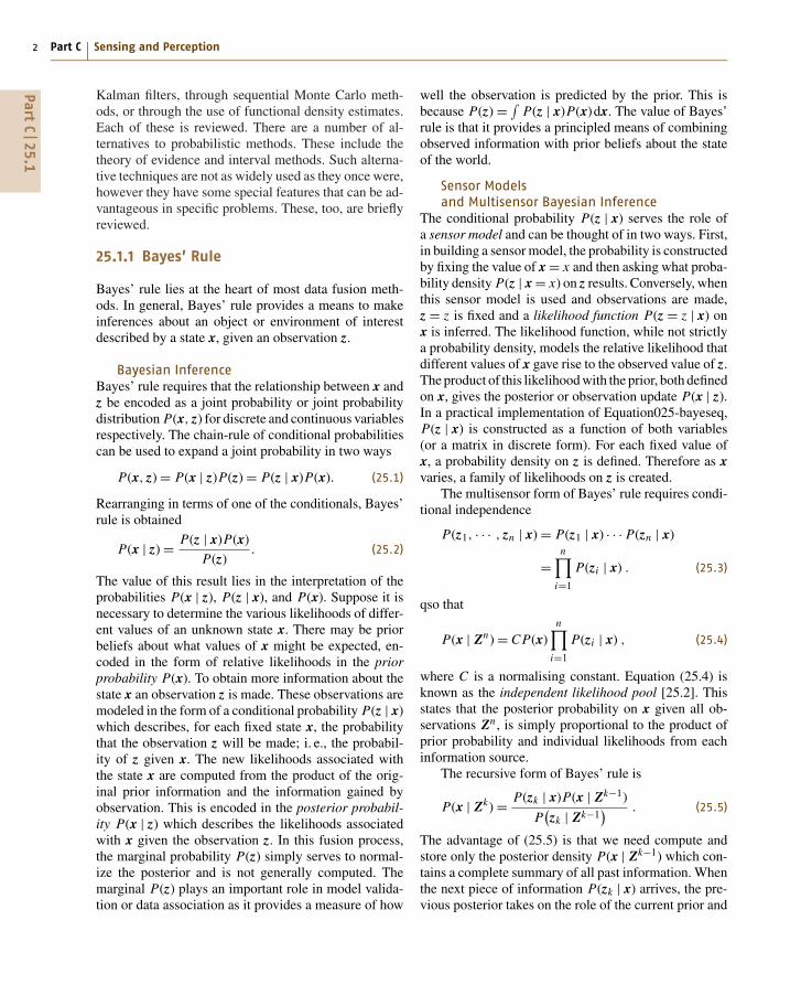
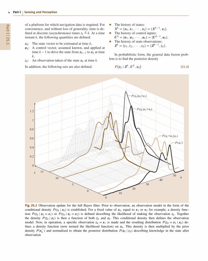
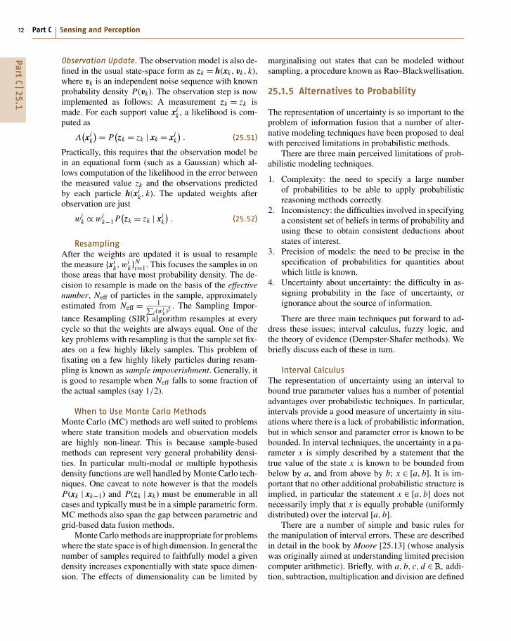
Fig. 25.1 Time update step for the full Bayes filter. At a time k −1, knowledge of the state xk−1 is summarised ina probability distribution P(xk−1). A vehicle model, in the form of a conditional probability density P(xk | xk−1), thendescribes the stochastic transition of the vehicle from a state xk−1 at a time k −1 to a state xk at a time k. Functionally,this state transition may be related to an underlying kinematic state model in the form xk = f (xk−1, uk). The figure showstwo typical conditional probability distributions P(xk | xk−1) on the state xk given fixed values of xk−1. The productof this conditional distribution with the marginal distribution P(xk−1), describing the prior likelihood of values of xk ,gives the the joint distribution P(xk, xk−1) shown as the surface in the figure. The total marginal density P(xk) describesknowledge of xk after state transition has occurred. The marginal density P(xk) is obtained by integrating (projecting) thejoint distribution P(xk, xk−1) over all xk−1. Equivalently, using the total probability theorem, the marginal density canbe obtained by integrating (summing) all conditional densities P(xk | xk−1) weighted by the prior probability P(xk−1) ofeach xk−1. The process can equally be run in reverse (a retroverse motion model) to obtain P(xk−1) from P(xk) givena model P(xk−1 | xk)
in tracking and navigation. The general filtering problemcan be formulated in Bayesian form. This is significantbecause it provides a common representation for a rangeof discrete and continuous data fusion problems withoutrecourse to specific target or observation models.
Define xt as the value of a state of interest at time t.This may, for example, describe a feature to be tracked,the state of a process being monitored, or the location
PartC
25.1
4 Part C Sensing and Perception
of a platform for which navigation data is required. Forconvenience, and without loss of generality, time is de-fined at discrete (asynchronous) times tk � k. At a timeinstant k, the following quantities are defined:
xk: The state vector to be estimated at time k,uk: A control vector, assumed known, and applied at
time k −1 to drive the state from xk−1 to xk at timek,
zk: An observation taken of the state xk at time k.
In addition, the following sets are also defined.
P (xk–)
P (zk |xk=x1)
0
10
20
30
40
50
0
5
10
15z
x
1.2
1
0.8
0.6
0.4
0.2
0
P (zk=x1 |xk)
P (zk |xk=x2)
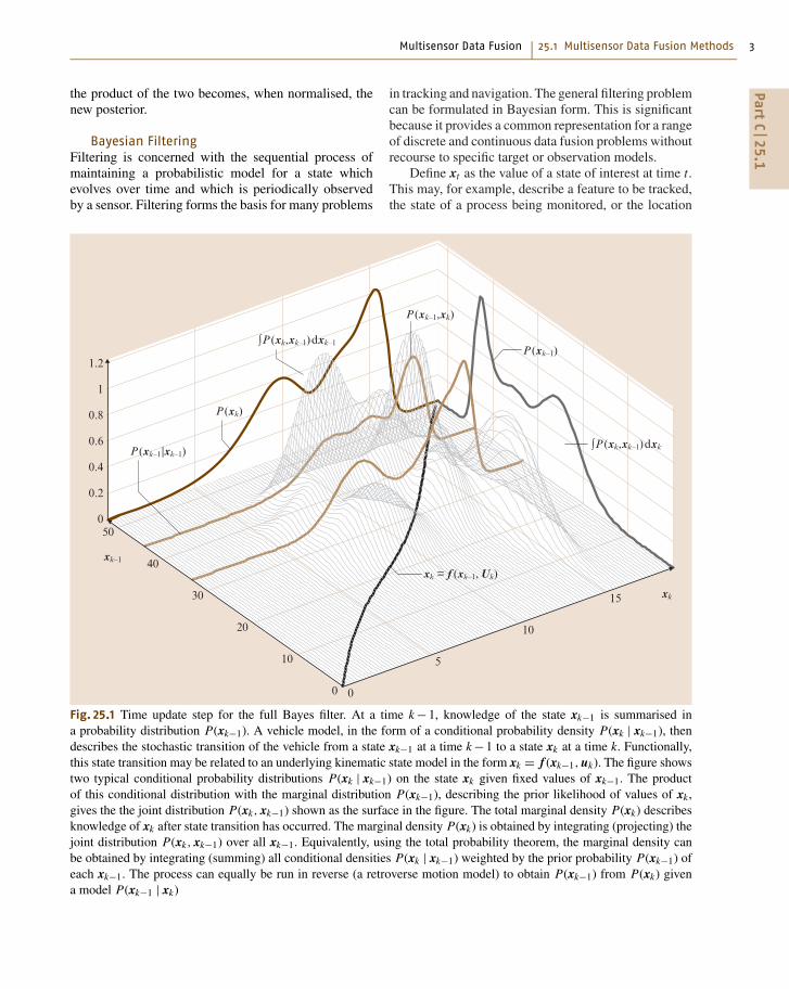
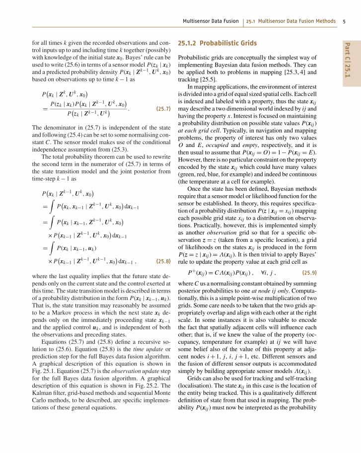
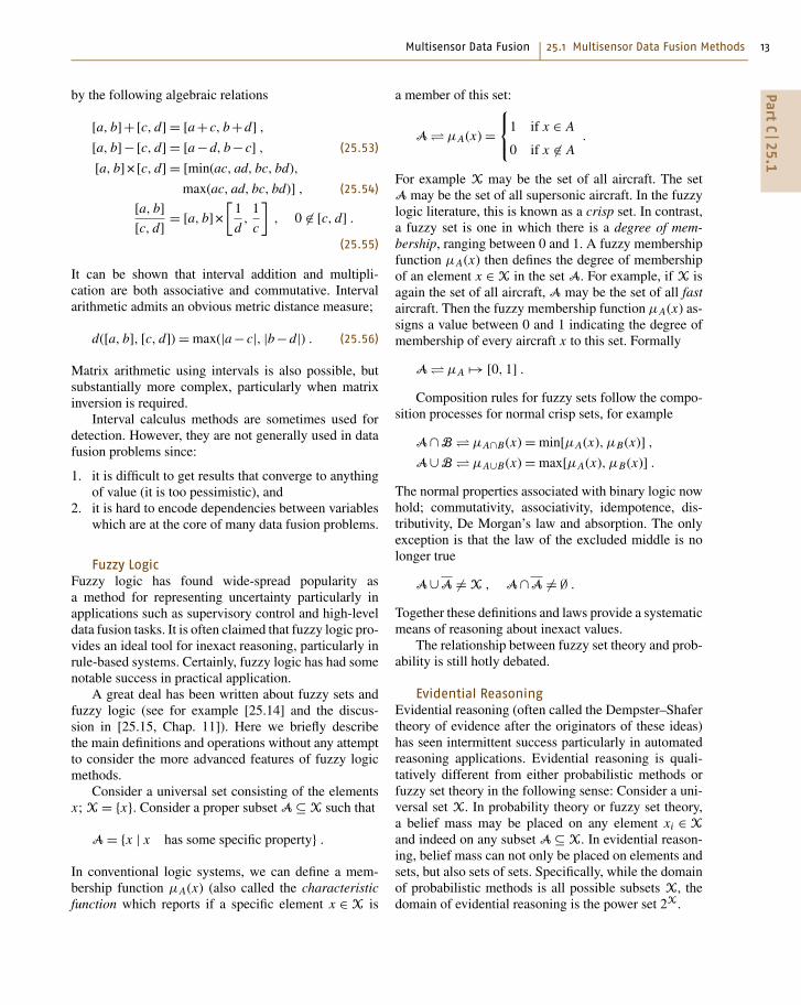
Fig. 25.2 Observation update for the full Bayes filter. Prior to observation, an observation model in the form of theconditional density P(zk | xk) is established. For a fixed value of xk , equal to x1 or x2 for example, a density func-tion P(zk | xk = x1) or P(zk | xk = x2) is defined describing the likelihood of making the observation zk. Togetherthe density P(zk | xk) is then a function of both zk and xk . This conditional density then defines the observationmodel. Now, in operation, a specific observation zk = x1 is made and the resulting distribution P(zk = x1 | xk) de-fines a density function (now termed the likelihood function) on xk . This density is then multiplied by the priordensity P(x−
k ) and normalised to obtain the posterior distribution P(xk | zk) describing knowledge in the state afterobservation
• The history of states:Xk = {x0, x1, · · · , xk} = {Xk−1, xk}.• The history of control inputs:Uk = {u1, u2, · · · , uk} = {Uk−1, uk}.• The history of state observations:Zk = {z1, z2, · · · , zk} = {Zk−1, zk}.
In probabilistic form, the general data fusion prob-lem is to find the posterior density
P(xk | Zk, Uk, x0
)(25.6)
PartC
25.1
Multisensor Data Fusion 25.1 Multisensor Data Fusion Methods 5
for all times k given the recorded observations and con-trol inputs up to and including time k together (possibly)with knowledge of the initial state x0. Bayes’ rule can beused to write (25.6) in terms of a sensor model P(zk | xk)and a predicted probability density P(xk | Zk−1, Uk, x0)based on observations up to time k −1 as
P(xk | Zk, Uk, x0
)
= P(zk | xk)P(xk | Zk−1, Uk, x0
)P(zk | Zk−1, Uk
) . (25.7)
The denominator in (25.7) is independent of the stateand following (25.4) can be set to some normalising con-stant C. The sensor model makes use of the conditionalindependence assumption from (25.3).
The total probability theorem can be used to rewritethe second term in the numerator of (25.7) in terms ofthe state transition model and the joint posterior fromtime-step k −1 as
P(xk | Zk−1, Uk, x0
)=
∫P(xk, xk−1 | Zk−1, Uk, x0
)dxk−1
=∫
P(xk | xk−1, Zk−1, Uk, x0
)× P
(xk−1 | Zk−1, Uk, x0
)dxk−1
=∫
P(xk | xk−1, uk)
× P(xk−1 | Zk−1, Uk−1, x0
)dxk−1 , (25.8)
where the last equality implies that the future state de-pends only on the current state and the control exerted atthis time. The state transition model is described in termsof a probability distribution in the form P(xk | xk−1, uk).That is, the state transition may reasonably be assumedto be a Markov process in which the next state xk de-pends only on the immediately proceeding state xk−1and the applied control uk, and is independent of boththe observations and preceding states.
Equations (25.7) and (25.8) define a recursive so-lution to (25.6). Equation (25.8) is the time update orprediction step for the full Bayes data fusion algorithm.A graphical description of this equation is shown inFig. 25.1. Equation (25.7) is the observation update stepfor the full Bayes data fusion algorithm. A graphicaldescription of this equation is shown in Fig. 25.2. TheKalman filter, grid-based methods and sequential MonteCarlo methods, to be described, are specific implemen-tations of these general equations.
25.1.2 Probabilistic Grids
Probabilistic grids are conceptually the simplest way ofimplementing Bayesian data fusion methods. They canbe applied both to problems in mapping [25.3, 4] andtracking [25.5].
In mapping applications, the environment of interestis divided into a grid of equal sized spatial cells. Each cellis indexed and labeled with a property, thus the state xijmay describe a two dimensional world indexed by ij andhaving the property x. Interest is focused on maintaininga probability distribution on possible state values P(xij )at each grid cell. Typically, in navigation and mappingproblems, the property of interest has only two valuesO and E, occupied and empty, respectively, and it isthen usual to assume that P(xij = O) = 1− P(xij = E).However, there is no particular constraint on the propertyencoded by the state xij which could have many values(green, red, blue, for example) and indeed be continuous(the temperature at a cell for example).
Once the state has been defined, Bayesian methodsrequire that a sensor model or likelihood function for thesensor be established. In theory, this requires specifica-tion of a probability distribution P(z | xij = xij ) mappingeach possible grid state xij to a distribution on observa-tions. Practically, however, this is implemented simplyas another observation grid so that for a specific ob-servation z = z (taken from a specific location), a gridof likelihoods on the states xij is produced in the formP(z = z | xij ) = Λ(xij ). It is then trivial to apply Bayes’rule to update the property value at each grid cell as
P+(xij ) = CΛ(xij )P(xij ) , ∀i, j , (25.9)
where C us a normalising constant obtained by summingposterior probabilities to one at node ij only. Computa-tionally, this is a simple point-wise multiplication of twogrids. Some care needs to be taken that the two grids ap-propriately overlap and align with each other at the rightscale. In some instances it is also valuable to encodethe fact that spatially adjacent cells will influence eachother; that is, if we knew the value of the property (oc-cupancy, temperature for example) at ij we will havesome belief also of the value of this property at adja-cent nodes i +1, j, i, j +1, etc. Different sensors andthe fusion of different sensor outputs is accommodatedsimply by building appropriate sensor models Λ(xij ).
Grids can also be used for tracking and self-tracking(localisation). The state xij in this case is the location ofthe entity being tracked. This is a qualitatively differentdefinition of state from that used in mapping. The prob-ability P(xij ) must now be interpreted as the probability
PartC
25.1
6 Part C Sensing and Perception
that the object being tracked occupies the grid cell ij. Inthe case of mapping, the sum of property probabilitiesat each grid cell is one, whereas in the case of tracking,the sum of location probabilities over the whole gridmust sum to one. Otherwise, the procedure for updat-ing is very similar. An observation grid is constructedwhich when instantiated with an observation value pro-vides a location likelihood grid P(z = z | xij ) = Λ(xij ).Bayes’ rule is then applied to update the location proba-bility at each grid cell in the same form as (25.9) exceptthat now the normalisation constant C is obtained bysumming posterior probabilities over all ij grid cells.This can become computationally expensive, especiallyif the grid has three or more dimensions. One majoradvantage of grid-based tracking is that it is easy to in-corporate quite complex prior information. For example,if it is known that the object being tracked is on a road,then the probability location values for all off-road gridcells can simply be set to zero.
Grid based fusion is appropriate to situations wherethe domain size and dimension are modest. In suchcases, grid based methods provide straightforward andeffective fusion algorithms. Grid based methods can beextended in a number of ways; to hierarchical (quad-tree) grids, or to irregular (triangular, pentagonal) grids.These can help reduce computation in larger spaces.Monte Carlo and particle filtering methods (Sect. 25.1.4)may be considered as grid-based methods, where thegrid cells themselves are sample of the underlying prob-ability density for the state.
25.1.3 The Kalman Filter
The Kalman filter is a recursive linear estimator whichsuccessively calculates an estimate for a continuous val-ued state, that evolves over time, on the basis of periodicobservations of the state. The Kalman filter employs anexplicit statistical model of how the parameter of in-terest x(t) evolves over time and an explicit statisticalmodel of how the observations z(t) that are made are re-lated to this parameter. The gains employed in a Kalmanfilter are chosen to ensure that, with certain assump-tions about the observation and process models used,the resulting estimate x(t) minimises mean-squared er-ror and is thus the conditional mean x(t) = E[x(t) | Zt];an average, rather than a most likely value.
The Kalman filter has a number of featureswhich make it ideally suited to dealing with complexmulti-sensor estimation and data fusion problems. Inparticular, the explicit description of process and ob-servations allows a wide variety of different sensor
models to be incorporated within the basic algorithm.In addition, the consistent use of statistical measures ofuncertainty makes it possible to quantitatively evaluatethe role each sensor plays in overall system performance.Further, the linear recursive nature of the algorithm en-sures that its application is simple and efficient. For thesereasons, the Kalman filter has found wide-spread appli-cation in many different data fusion problems [25.6–9].
In robotics, the Kalman filter is most suited to prob-lems in tracking, localisation and navigation; and lessso to problems in mapping. This is because the algo-rithm works best with well defined state descriptions(positions, velocities, for example), and for states whereobservation and time-propagation models are also wellunderstood.
Observation and Transition ModelsThe Kalman filter may be considered a specific instanceof the recursive Bayesian filter of (25.7,25.8) for the casewhere the probability densities on states are Gaussian.The starting point for the Kalman Filter algorithm isto define a model for the states to be estimated in thestandard state-space form:
x(t) = F(t)x(t)+ B(t)u(t)+ G(t)v(t) , (25.10)
where x(t) is the state vector of interest, u(t) is a knowncontrol input, v(t) is a random variable describing un-certainty in the evolution of the state, and where F(t),B(t), and G(t) are matrices describing the contributionof states, controls and noise to state transition [25.7]. Anobservation (output) model is also defined in standardstate-space form:
z(t) = H(t)x(t)+ D(t)w(t) , (25.11)
where z(t) is the observation vector, w(t) is a ran-dom variable describing uncertainty in the observation,and where H(t) and D(t) are matrices describing thecontribution of state and noise to the observation.
These equations define the evolution of a continuous-time system with continuous observations being made ofthe state. However, the Kalman Filter is almost alwaysimplemented in discrete-time tk = k. It is straightfor-ward [25.8] to obtain a discrete-time version of (25.10)and (25.11) in the form
x(k) = F(k)x(k −1)+ B(k)u(k)+ G(k)v(k) ,
(25.12)
z(k) = H(k)x(k)+ D(k)w(k) . (25.13)
A basic assumption in the derivation of the Kalmanfilter is that the random sequences v(k) and w(k) de-scribing process and observation noise are all Gaussian,
PartC
25.1
Multisensor Data Fusion 25.1 Multisensor Data Fusion Methods 7
temporally uncorrelated and zero-mean
E[v(k)] = E[w(k)] = 0 , ∀k , (25.14)
with known covariance
E[v(i)vT( j)] = δij Q(i) , E[w(i)wT( j)] = δij R(i) .
(25.15)
It is also generally assumed that the process and obser-vation noises are also uncorrelated
E[v(i)wT( j)] = 0 , ∀i, j . (25.16)
These are equivalent to a Markov property requiringobservations and successive states to be conditionallyindependent. If the sequences v(k) and w(k) are tempo-rally correlated, a shaping filter can be used to whiten theobservations, again making the assumptions required forthe Kalman filter valid [25.8]. If the process and observa-tion noise sequences are correlated, then this correlationcan also be accounted for in the Kalman filter algo-rithm [25.10]. If the sequence is not Gaussian, but issymmetric with finite moments, then the Kalman filterwill still produce good estimates. If however, the se-quence has a distribution which is skewed or otherwisepathological, results produced by the Kalman filter willbe misleading and there will be a good case for usinga more sophisticated Bayesian filter [25.5].
Filtering AlgorithmThe Kalman filter algorithm produces estimates thatminimise mean-squared estimation error conditioned ona given observation sequence and so is the conditionalmean
x(i | j)� E[x(i) | z(1), · · · , z( j)]� E[x(i) | Z j ] .
(25.17)
The estimate variance is defined as the mean-squarederror in this estimate
P(i | j)� E{[x(i)− x(i | j)][x(i)− x(i | j)]T | Z j} .
(25.18)
The estimate of the state at a time k given all informationup to time k is written as x(k | k). The estimate of thestate at a time k given only information up to time k −1 iscalled a one-step-ahead prediction (or just a prediction)and is written as x(k | k −1).
The Kalman filter algorithm is now stated withoutproof. Detailed derivations can be found in many bookson the subject, [25.7,8] for example. The state is assumedto evolve in time according to (25.12). Observations ofthis state are made at regular time intervals according
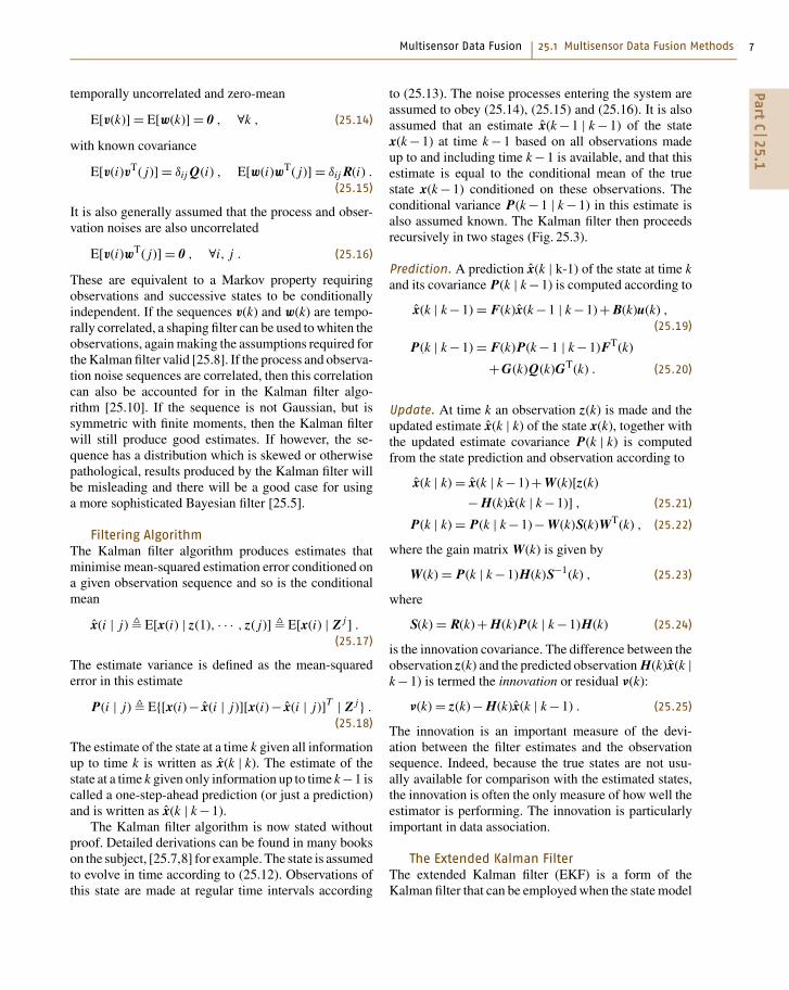
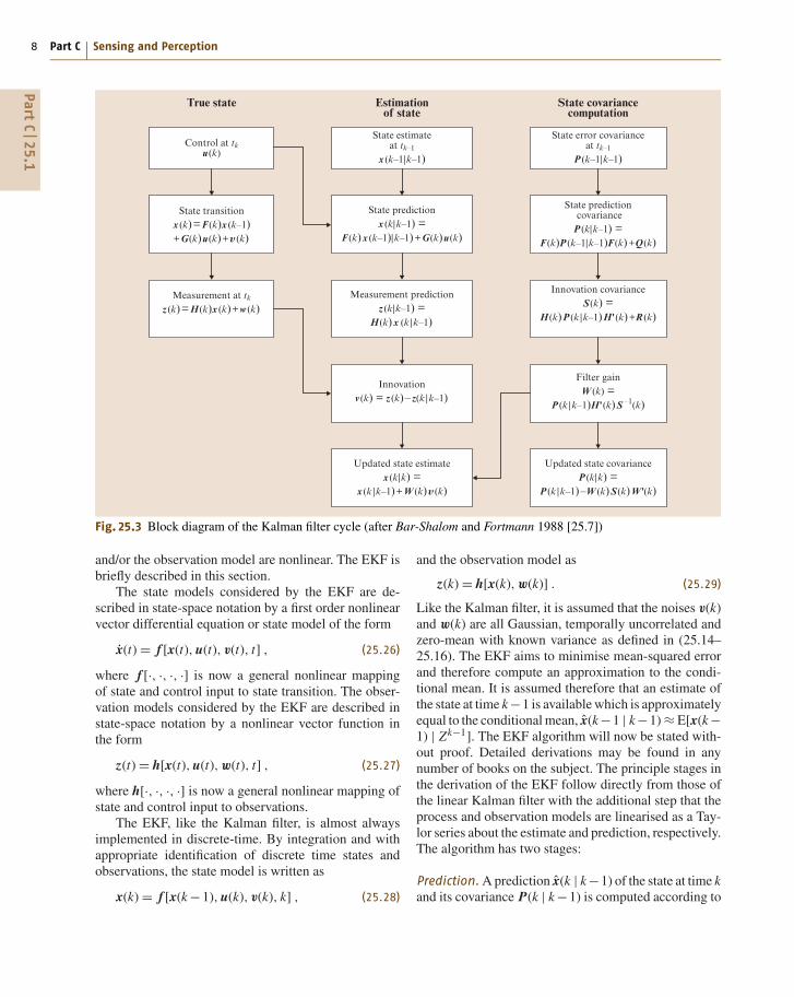
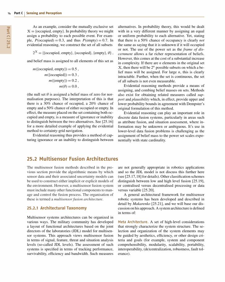
to (25.13). The noise processes entering the system areassumed to obey (25.14), (25.15) and (25.16). It is alsoassumed that an estimate x(k −1 | k −1) of the statex(k −1) at time k −1 based on all observations madeup to and including time k −1 is available, and that thisestimate is equal to the conditional mean of the truestate x(k −1) conditioned on these observations. Theconditional variance P(k −1 | k −1) in this estimate isalso assumed known. The Kalman filter then proceedsrecursively in two stages (Fig. 25.3).
Prediction. A prediction x(k | k-1) of the state at time kand its covariance P(k | k −1) is computed according to
x(k | k −1) = F(k)x(k −1 | k −1)+ B(k)u(k) ,
(25.19)
P(k | k −1) = F(k)P(k −1 | k −1)FT(k)
+ G(k)Q(k)GT(k) . (25.20)
Update. At time k an observation z(k) is made and theupdated estimate x(k | k) of the state x(k), together withthe updated estimate covariance P(k | k) is computedfrom the state prediction and observation according to
x(k | k) = x(k | k −1)+ W(k)[z(k)
− H(k)x(k | k −1)] , (25.21)
P(k | k) = P(k | k −1)− W(k)S(k)WT(k) , (25.22)
where the gain matrix W(k) is given by
W(k) = P(k | k −1)H(k)S−1(k) , (25.23)
where
S(k) = R(k)+ H(k)P(k | k −1)H(k) (25.24)
is the innovation covariance. The difference between theobservation z(k) and the predicted observation H(k)x(k |k −1) is termed the innovation or residual ν(k):
ν(k) = z(k)− H(k)x(k | k −1) . (25.25)
The innovation is an important measure of the devi-ation between the filter estimates and the observationsequence. Indeed, because the true states are not usu-ally available for comparison with the estimated states,the innovation is often the only measure of how well theestimator is performing. The innovation is particularlyimportant in data association.
The Extended Kalman FilterThe extended Kalman filter (EKF) is a form of theKalman filter that can be employed when the state model
PartC
25.1
8 Part C Sensing and Perception
True state
Control at tku (k)
Estimationof state
State estimateat tk–1
x (k–1|k–1)
State covariancecomputation
State error covarianceat tk–1
P (k–1|k–1)
State transitionx (k)=F (k)x (k–1)+G (k)u (k)+υ (k)
State predictionx (k|k–1) =
F (k)x (k–1)|k–1)+G (k)u (k)
State prediction covarianceP (k|k–1) =
F (k)P (k–1|k–1)F (k)+Q (k)
Innovationv (k) = z (k)–z(k |k–1)
Filter gainW (k) =
P (k |k–1)H' (k)S –1(k)
Updated state estimatex (k|k) =
x (k |k–1)+W (k)υ (k)
Updated state covarianceP (k|k) =
P (k |k–1)–W (k)S (k)W'(k)
Measurement at tkz (k)=H (k)x (k)+w (k)
Measurement predictionz (k|k–1) =
H (k)x (k |k–1)
Innovation covarianceS (k) =
H (k)P (k |k–1)H' (k)+R (k)
Fig. 25.3 Block diagram of the Kalman filter cycle (after Bar-Shalom and Fortmann 1988 [25.7])
and/or the observation model are nonlinear. The EKF isbriefly described in this section.
The state models considered by the EKF are de-scribed in state-space notation by a first order nonlinearvector differential equation or state model of the form
x(t) = f [x(t), u(t), v(t), t] , (25.26)
where f [·, ·, ·, ·] is now a general nonlinear mappingof state and control input to state transition. The obser-vation models considered by the EKF are described instate-space notation by a nonlinear vector function inthe form
z(t) = h[x(t), u(t),w(t), t] , (25.27)
where h[·, ·, ·, ·] is now a general nonlinear mapping ofstate and control input to observations.
The EKF, like the Kalman filter, is almost alwaysimplemented in discrete-time. By integration and withappropriate identification of discrete time states andobservations, the state model is written as
x(k) = f [x(k −1), u(k), v(k), k] , (25.28)
and the observation model as
z(k) = h[x(k),w(k)] . (25.29)
Like the Kalman filter, it is assumed that the noises v(k)and w(k) are all Gaussian, temporally uncorrelated andzero-mean with known variance as defined in (25.14–25.16). The EKF aims to minimise mean-squared errorand therefore compute an approximation to the condi-tional mean. It is assumed therefore that an estimate ofthe state at time k −1 is available which is approximatelyequal to the conditional mean, x(k −1 | k −1) ≈ E[x(k −1) | Zk−1]. The EKF algorithm will now be stated with-out proof. Detailed derivations may be found in anynumber of books on the subject. The principle stages inthe derivation of the EKF follow directly from those ofthe linear Kalman filter with the additional step that theprocess and observation models are linearised as a Tay-lor series about the estimate and prediction, respectively.The algorithm has two stages:
Prediction. A prediction x(k | k −1) of the state at time kand its covariance P(k | k −1) is computed according to
PartC
25.1
Multisensor Data Fusion 25.1 Multisensor Data Fusion Methods 9
x(k | k −1) = f [x(k −1 | k −1), u(k)] , (25.30)
P(k | k −1) = ∇ fx(k)P(k −1 | k −1)∇T fx(k)
+∇ fv(k)Q(k)∇T fv(k) . (25.31)
Update. At time k an observation z(k) is made and theupdated estimate x(k | k) of the state x(k), together withthe updated estimate covariance P(k | k) is computedfrom the state prediction and observation according to
x(k | k) = x(k | k −1)
+ W(k){z(k)−h[x(k | k −1)]} , (25.32)
P(k | k) = P(k | k −1)− W(k)S(k)WT, (k) , (25.33)
where
W(k) = P(k | k −1)∇Thx(k)S−1(k) (25.34)
and
S(k) = ∇hw(k)R(k)∇Thw(k)
+∇hx(k)P(k | k −1)∇Thx(k) (25.35)
and where the Jacobian ∇ f·(k) is evaluated at x(k −1) =x(k −1 | k −1) and ∇h·(k) is evaluated at and x(k) =x(k | k −1).
A comparison of (25.19–25.24) with (25.30–25.35)makes it clear that the EKF algorithm is very similar tothe linear Kalman filter algorithm, with the substitutionsF(k) → ∇ fx(k) and H(k) → ∇hx(k) being made in theequations for the variance and gain propagation. Thus,the EKF is, in effect, a linear estimator for a state errorwhich is described by a linear equation and which isbeing observed according to a linear equation of theform of (25.13).
The EKF works in much the same way as the linearKalman filter with some notable caveats.
• The Jacobians ∇ fx(k) and ∇hx(k) are typically notconstant, being functions of both state and timestep.This means that unlike the linear filter, the covari-ances and gain matrix must be computed on-line asestimates and predictions are made available, andwill not in general tend to constant values. Thissignificantly increases the amount of computationwhich must be performed on-line by the algorithm.• As the linearised model is derived by perturbing thetrue state and observation models around a predictedor nominal trajectory, great care must be taken to en-sure that these predictions are always close enoughto the true state that second order terms in the lin-earisation are indeed insignificant. If the nominaltrajectory is too far away from the true trajectory
then the true covariance will be much larger thanthe estimated covariance and the filter will becomepoorly matched. In extreme cases the filter may alsobecome unstable.• The EKF employs a linearised model which mustbe computed from an approximate knowledge ofthe state. Unlike the linear algorithm, this meansthat the filter must be accurately initialized at thestart of operation to ensure that the linearised modelsobtained are valid. If this is not done, the estimatescomputed by the filter will simply be meaningless.
The Information FilterThe information filter is mathematically equivalent toa Kalman filter. However, rather than generating stateestimates x(i | j) and covariances P(i | j) it uses infor-mation state variables y(i | j) and information matricesY(i | j) which are related to each other through therelationships
y(i | j) = P−1(i | j)x(i | j) , Y(i | j) = P−1(i | j) .
(25.36)
The information filter has the same prediction-updatestructure as the Kalman filter.
Prediction. A prediction y(k | k −1) of the informationstate at time k and its information matrix Y(k | k −1) iscomputed according to (Joseph form [25.8]):
y(k | k −1) = (1−ΩGT)F−T y(k −1 | k −1)
+Y(k | k −1)Bu(k) , (25.37)
Y(k | k −1) = M(k)−ΩΣΩT , (25.38)
respectively, where
M(k) = F−T Y(k −1 | k −1)F−1 ,
Σ = GT M(k)G + Q−1 ,
and
Ω = M(tk)GΣ−1 .
It should be noted that Σ , whose inverse is required tocompute Ω, is only of dimension of the process drivingnoise which is normally considerably smaller than thestate dimension. Further, the matrix F−1 is the state-transition matrix evaluated backwards in time and somust always exist.
Update. At time k an observation z(k) is made and theupdated information state estimate y(k | k) together with
PartC
25.1
10 Part C Sensing and Perception
the updated information matrix Y(k | k) is computedfrom
y(k | k) = y(k | k −1)+ H(k)R−1(k)z(k) , (25.39)
Y(k | k) = Y(k | k −1)+ H(k)R−1(k)HT(k). (25.40)
We emphasise that (25.38) and (25.37) are math-ematically identical to (25.19) and (25.20), and that(25.39) and (25.40) are mathematically identical to(25.21) and (25.22). It will be noted that there is a dual-ity between information and state space forms [25.10].This duality is evident from the fact that Ω and Σ in theprediction stage of the information filter play an equiva-lent role to the gain matrix W and innovation covarianceS in the update stage of the Kalman filter. Further, thesimple linear update step for the information filter is mir-rored in the simple linear prediction step for the Kalmanfilter.
The main advantage of the information filter over theKalman filter in data fusion problems is the relative sim-plicity of the update stage. For a system with n sensors,the fused information state update is exactly the linearsum of information contributions from all sensors as
y(k | k) = y(k | k −1)+n∑
i=1
Hi (k)R−1i (k)zi (k) ,
Y(k | k) = Y(k | k −1)+n∑
i=1
Hi (k)R−1i (k)HT
i (k) .
(25.41)
The reason such an expression exists in this form is thatthe information filter is essentially a log-likelihood ex-pression of Bayes’ rule, where products of likelihoods(25.4) are turned into sums. No such simple expressionfor multi-sensor updates exists for the Kalman Filter.This property of the information filter has been ex-ploited for data fusion in robotic networks [25.11, 12]and more recently in robot navigation and localisationproblems [25.1]. One substantial disadvantage of theinformation filter is the coding of nonlinear models,especially for the prediction step.
When to Use a Kalman or Information FilterKalman or information filters are appropriate to data fu-sion problems where the entity of interest is well definedby a continuous parametric state. This would include es-timation of the position, attitude and velocity of a robotor other object, or the tracking of a simple geometricfeature such as a point, line or curve. Kalman and infor-mation filters are inappropriate for estimating propertiessuch as spatial occupancy, discrete labels, or processeswhose error characteristics are not easily parametrised.
25.1.4 Sequential Monte Carlo Methods
Monte Carlo (MC) filter methods describe probabilitydistributions as a set of weighted samples of an underly-ing state space. MC filtering then uses these samples tosimulate probabilistic inference usually through Bayes’rule. Many samples or simulations are performed. Bystudying the statistics of these samples as they progressthrough the inference process, a probabilistic picture ofthe process being simulated can be built up.
Representing Probability DistributionsIn sequential Monte Carlo methods, probability dis-tributions are described in terms of a set of supportpoints (state space values) xi , i = 1, · · · , N , togetherwith a corresponding set of normalised weights wi ,i = 1, · · · , N , where
∑i wi = 1. The support points
and weights can be used to define a probability densityfunction in the form
P(x) ≈N∑
i=1
wiδ(x− xi ) . (25.42)
A key question is how these support points and weightsare selected to obtain a faithful representation of theprobability density P(x). The most general way of se-lecting support values is to use an importance densityq(x). The support values xi are drawn as samples fromthis density; where the density has high probability, moresupport values are chosen, and where the density has lowprobability, few support support vectors are selected.The weights in (25.42) are then computed from
wi ∝ P(xi )
q(xi ). (25.43)
Practically, a sample xi is drawn from the importancedistribution. The sample is then instantiated in theunderlying probability distribution to yield the valueP(x = xi ). The ratio of the two probability values,appropriately normalised, then becomes the weight.
There are two instructive extremes of the importancesampling method.
1. At one extreme, the importance density could betaken to be a uniform distribution and so the sup-port values xi are uniformly distributed on the statespace in a close approximation to a grid. The prob-abilities q(xi ) are also therefore equal. The weightscomputed from (25.43) are then simply proportionalto the probabilities wi ∝ P(x = xi ). The result isa model for the distribution which looks very likethe regular grid model.
PartC
25.1
Multisensor Data Fusion 25.1 Multisensor Data Fusion Methods 11
2. At the other extreme, we could choose an importancedensity equal to the probability model q(x) = P(x).Samples of the support values xi are now drawn fromthis density. Where the density is high there will bemany samples, where the density is low there willbe few samples. However, if we substitute q(xi ) =P(xi ) into (25.43), it is clear that the weights allbecome equal wi = 1/N . A set of samples with equalweights is known as a particle distribution.
It is, of course, possible to mix these two representa-tions to describe a probability distribution both in termsof a set of weights and in terms of a set of support val-ues. The complete set of samples and weights describinga probability distribution {xi , wi}N
i=1 is termed a randommeasure.
The Sequential Monte Carlo MethodSequential Monte Carlo (SMC) filtering is a simulationof the recursive Bayes update equations using samplesupport values and weights to describe the underlyingprobability distributions.
The starting point is the recursive or sequentialBayes observation update given in (25.7) and (25.8).The SMC recursion begins with a posterior probabil-ity density represented by a set of support values andweights {xi
k−1, wik−1|k−1}Nk−1
i=1 in the form
P(xk−1 | Zk−1) =
Nk−1∑i=1
wik−1δ
(xk−1 − xi
k−1
). (25.44)
The prediction step requires that (25.44) is substitutedinto (25.8) where the joint density is marginalised.Practically however, this complex step is avoided by im-plicitly assuming that the importance density is exactlythe transition model as
qk(xi
k
) = P(xi
k | xik−1
). (25.45)
This allows new support values xik to be drawn on
the basis of old support values xik−1 while leaving the
weights unchanged wik = wi
k−1. With this, the predictionbecomes
P(xk | Zk−1) =
Nk∑i=1
wik−1δ
(xk − xi
k
). (25.46)
The SMC observation update step is relatively straight-forward. An observation model P(zk | xk) is defined.This is a function on both variables, zk and xk,and is a probability distribution on zk (integratesto unity). When an observation or measurement is
made, zk = zk, the observation model becomes a func-tion of state xk only. If samples of the state aretaken xk = xi
k, i = 1 · · · , Nk, the observation modelP(zk = zk | xk = xi
k) becomes a set of scalars describ-ing the likelihood that the sample xi
k could have givenrise to the observation zk. Substituting these likelihoodsand (25.46) into (25.7) gives:
P(xk | Zk)
= CNk∑
i=1
wik−1 P
(zk = zk | xk = xi
k
)δ(xk − xi
k
).
(25.47)
This is normally implemented in the form of an updatedset of normalised weights
wik = wi
k−1 P(zk = zk | xk = xi
k
)∑Nk
j=1 wjk−1 P
(zk = zk | xk = x j
k
) (25.48)
and so
P(xk | Zk) =
Nk∑i=1
wikδ
(xk − xi
k
). (25.49)
Note that the support values in (25.49) are the same asthose in (25.46), only the weights have been changed bythe observation update.
The implementation of the SMC method requires theenumeration of models for both state transition P(xk |xk−1) and the observation P(zk | xk). These need to bepresented in a form that allows instantiation of valuesfor zk, xk and xk−1. For low dimensional state spaces,interpolation in a lookup table is a viable representation.For high dimensional state spaces, the preferred methodis to provide a representation in terms of a function.
Practically, (25.46) and (25.49) are implemented asfollows:
Time Update. A process model is defined in the usualstate-space form as xk = f (xk−1,wk−1, k), where wk isan independent noise sequence with known probabilitydensity P(wk). The prediction step is now implementedas follows: Nk samples wi
k, i = 1, · · · , Nk are drawnfrom the distribution P(wk). The Nk support values xi
k−1together with the samples wi
k are passed through theprocess model as
xik = f
(xi
k−1,wik−1, k
)(25.50)
yielding a new set of support vectors xik. The weights for
these support vectors wik−1 are not changed. In effect,
the process model is simply used to do Nk simulationsof state propagation.
PartC
25.1
12 Part C Sensing and Perception
Observation Update. The observation model is also de-fined in the usual state-space form as zk = h(xk, vk, k),where vk is an independent noise sequence with knownprobability density P(vk). The observation step is nowimplemented as follows: A measurement zk = zk ismade. For each support value xi
k, a likelihood is com-puted as
Λ(xi
k
) = P(zk = zk | xk = xi
k
). (25.51)
Practically, this requires that the observation model bein an equational form (such as a Gaussian) which al-lows computation of the likelihood in the error betweenthe measured value zk and the observations predictedby each particle h(xi
k, k). The updated weights afterobservation are just
wik ∝ wi
k−1 P(zk = zk | xi
k
). (25.52)
ResamplingAfter the weights are updated it is usual to resamplethe measure {xi
k, wik}N
i=1. This focuses the samples in onthose areas that have most probability density. The de-cision to resample is made on the basis of the effectivenumber, Neff of particles in the sample, approximatelyestimated from Neff = 1∑
i (wik)2 . The Sampling Impor-
tance Resampling (SIR) algorithm resamples at everycycle so that the weights are always equal. One of thekey problems with resampling is that the sample set fix-ates on a few highly likely samples. This problem offixating on a few highly likely particles during resam-pling is known as sample impoverishment. Generally, itis good to resample when Neff falls to some fraction ofthe actual samples (say 1/2).
When to Use Monte Carlo MethodsMonte Carlo (MC) methods are well suited to problemswhere state transition models and observation modelsare highly non-linear. This is because sample-basedmethods can represent very general probability densi-ties. In particular multi-modal or multiple hypothesisdensity functions are well handled by Monte Carlo tech-niques. One caveat to note however is that the modelsP(xk | xk−1) and P(zk | xk) must be enumerable in allcases and typically must be in a simple parametric form.MC methods also span the gap between parametric andgrid-based data fusion methods.
Monte Carlo methods are inappropriate for problemswhere the state space is of high dimension. In general thenumber of samples required to faithfully model a givendensity increases exponentially with state space dimen-sion. The effects of dimensionality can be limited by
marginalising out states that can be modeled withoutsampling, a procedure known as Rao–Blackwellisation.
25.1.5 Alternatives to Probability
The representation of uncertainty is so important to theproblem of information fusion that a number of alter-native modeling techniques have been proposed to dealwith perceived limitations in probabilistic methods.
There are three main perceived limitations of prob-abilistic modeling techniques.
1. Complexity: the need to specify a large numberof probabilities to be able to apply probabilisticreasoning methods correctly.
2. Inconsistency: the difficulties involved in specifyinga consistent set of beliefs in terms of probability andusing these to obtain consistent deductions aboutstates of interest.
3. Precision of models: the need to be precise in thespecification of probabilities for quantities aboutwhich little is known.
4. Uncertainty about uncertainty: the difficulty in as-signing probability in the face of uncertainty, orignorance about the source of information.
There are three main techniques put forward to ad-dress these issues; interval calculus, fuzzy logic, andthe theory of evidence (Dempster-Shafer methods). Webriefly discuss each of these in turn.
Interval CalculusThe representation of uncertainty using an interval tobound true parameter values has a number of potentialadvantages over probabilistic techniques. In particular,intervals provide a good measure of uncertainty in situ-ations where there is a lack of probabilistic information,but in which sensor and parameter error is known to bebounded. In interval techniques, the uncertainty in a pa-rameter x is simply described by a statement that thetrue value of the state x is known to be bounded frombelow by a, and from above by b; x ∈ [a, b]. It is im-portant that no other additional probabilistic structure isimplied, in particular the statement x ∈ [a, b] does notnecessarily imply that x is equally probable (uniformlydistributed) over the interval [a, b].
There are a number of simple and basic rules forthe manipulation of interval errors. These are describedin detail in the book by Moore [25.13] (whose analysiswas originally aimed at understanding limited precisioncomputer arithmetic). Briefly, with a, b, c, d ∈ , addi-tion, subtraction, multiplication and division are defined
PartC
25.1
Multisensor Data Fusion 25.1 Multisensor Data Fusion Methods 13
by the following algebraic relations
[a, b]+ [c, d] = [a + c, b+d] ,
[a, b]− [c, d] = [a −d, b− c] , (25.53)
[a, b]× [c, d] = [min(ac, ad, bc, bd),
max(ac, ad, bc, bd)] , (25.54)
[a, b][c, d] = [a, b]×
[1
d,
1
c
], 0 �∈ [c, d] .
(25.55)
It can be shown that interval addition and multipli-cation are both associative and commutative. Intervalarithmetic admits an obvious metric distance measure;
d([a, b], [c, d]) = max(|a − c|, |b−d|) . (25.56)
Matrix arithmetic using intervals is also possible, butsubstantially more complex, particularly when matrixinversion is required.
Interval calculus methods are sometimes used fordetection. However, they are not generally used in datafusion problems since:
1. it is difficult to get results that converge to anythingof value (it is too pessimistic), and
2. it is hard to encode dependencies between variableswhich are at the core of many data fusion problems.
Fuzzy LogicFuzzy logic has found wide-spread popularity asa method for representing uncertainty particularly inapplications such as supervisory control and high-leveldata fusion tasks. It is often claimed that fuzzy logic pro-vides an ideal tool for inexact reasoning, particularly inrule-based systems. Certainly, fuzzy logic has had somenotable success in practical application.
A great deal has been written about fuzzy sets andfuzzy logic (see for example [25.14] and the discus-sion in [25.15, Chap. 11]). Here we briefly describethe main definitions and operations without any attemptto consider the more advanced features of fuzzy logicmethods.
Consider a universal set consisting of the elementsx; X = {x}. Consider a proper subset A ⊆ X such that
A = {x | x has some specific property} .
In conventional logic systems, we can define a mem-bership function μA(x) (also called the characteristicfunction which reports if a specific element x ∈ X is
a member of this set:
A� μA(x) =⎧⎨⎩
1 if x ∈ A
0 if x �∈ A.
For example X may be the set of all aircraft. The setA may be the set of all supersonic aircraft. In the fuzzylogic literature, this is known as a crisp set. In contrast,a fuzzy set is one in which there is a degree of mem-bership, ranging between 0 and 1. A fuzzy membershipfunction μA(x) then defines the degree of membershipof an element x ∈ X in the set A. For example, if X isagain the set of all aircraft, A may be the set of all fastaircraft. Then the fuzzy membership function μA(x) as-signs a value between 0 and 1 indicating the degree ofmembership of every aircraft x to this set. Formally
A� μA → [0, 1] .
Composition rules for fuzzy sets follow the compo-sition processes for normal crisp sets, for example
A∩B� μA∩B(x) = min[μA(x), μB(x)] ,
A∪B� μA∪B(x) = max[μA(x), μB(x)] .
The normal properties associated with binary logic nowhold; commutativity, associativity, idempotence, dis-tributivity, De Morgan’s law and absorption. The onlyexception is that the law of the excluded middle is nolonger true
A∪A �= X , A∩A �= ∅ .
Together these definitions and laws provide a systematicmeans of reasoning about inexact values.
The relationship between fuzzy set theory and prob-ability is still hotly debated.
Evidential ReasoningEvidential reasoning (often called the Dempster–Shafertheory of evidence after the originators of these ideas)has seen intermittent success particularly in automatedreasoning applications. Evidential reasoning is quali-tatively different from either probabilistic methods orfuzzy set theory in the following sense: Consider a uni-versal set X. In probability theory or fuzzy set theory,a belief mass may be placed on any element xi ∈ Xand indeed on any subset A ⊆ X. In evidential reason-ing, belief mass can not only be placed on elements andsets, but also sets of sets. Specifically, while the domainof probabilistic methods is all possible subsets X, thedomain of evidential reasoning is the power set 2X.
PartC
25.1
14 Part C Sensing and Perception
As an example, consider the mutually exclusive setX = {occupied, empty}. In probability theory we mightassign a probability to each possible event. For exam-ple, P(occupied) = 0.3, and thus P(empty) = 0.7. Inevidential reasoning, we construct the set of all subsets
2X = {{occupied, empty}, {occupied}, {empty},∅} ,
and belief mass is assigned to all elements of this set as
m({occupied, empty}) = 0.5 ,
m({occupied}) = 0.3 ,
m({empty}) = 0.2 ,
m(∅) = 0.0 ,
(the null set ∅ is assigned a belief mass of zero for nor-malisation purposes). The interpretation of this is thatthere is a 30% chance of occupied, a 20% chance ofempty and a 50% chance of either occupied or empty. Ineffect, the measure placed on the set containing both oc-cupied and empty, is a measure of ignorance or inabilityto distinguish between the two alternatives. See [25.16]for a more detailed example of applying the evidentialmethod to certainty-grid navigation.
Evidential reasoning thus provides a method of cap-turing ignorance or an inability to distinguish between
alternatives. In probability theory, this would be dealtwith in a very different manner by assigning an equalor uniform probability to each alternative. Yet, statingthat there is a 50% chance of occupancy is clearly notthe same as saying that it is unknown if it will occupiedor not. The use of the power set as the frame of dis-cernment allows a far richer representation of beliefs.However, this comes at the cost of a substantial increasein complexity. If there are n elements in the original setX, then there will be 2n possible subsets on which a be-lief mass will be assigned. For large n, this is clearlyintractable. Further, when the set is continuous, the setof all subsets is not even measurable.
Evidential reasoning methods provide a means ofassigning, and combing belief masses on sets. Methodsalso exist for obtaining related measures called sup-port and plausibility which, in effect, provide upper andlower probability bounds in agreement with Dempster’soriginal formulation of this method.
Evidential reasoning can play an important role indiscrete data fusion systems, particularly in areas suchas attribute fusion, and situation assessment, where in-formation may be unknown or ambiguous. It’s use inlower-level data fusion problems is challenging as theassignment of belief mass to the power set scales expo-nentially with state cardinality.
25.2 Multisensor Fusion Architectures
The multisensor fusion methods described in the pre-vious section provide the algorithmic means by whichsensor data and their associated uncertainty models canbe used to construct either implicit or explicit models ofthe environment. However, a multisensor fusion systemmust include many other functional components to man-age and control the fusion process. The organisation ofthese is termed a multisensor fusion architecture.
25.2.1 Architectural Taxonomy
Multisensor systems architectures can be organized invarious ways. The military community has developeda layout of functional architectures based on the jointdirectors of the laboratories (JDL) model for multisen-sor systems. This approach views multisensor fusionin terms of signal, feature, threat and situation analysislevels (so-called JDL levels). The assessment of suchsystems is specified in terms of tracking performance,survivability, efficiency and bandwidth. Such measures
are not generally appropriate in robotics applicationsand so the JDL model is not discuss this further here(see [25.17,18] for details). Other classification schemesdistinguish between low and high level fusion [25.19],or centralised versus decentralised processing or dataversus variable [25.20].
A general architectural framework for multisensorrobotic systems has been developed and described indetail by Makarenko [25.21], and we will base our dis-cussion on his approach. A system architecture is definedin terms of:
Meta Architecture. A set of high-level considerationsthat strongly characterize the system structure. The se-lection and organization of the system elements maybe guided by aesthetics, efficiency, or other design cri-teria and goals (for example, system and componentcomprehensibility, modularity, scalability, portability,interoperability, (de)centralization, robustness, fault tol-erance).
PartC
25.2
Multisensor Data Fusion 25.2 Multisensor Fusion Architectures 15
Algorithmic Architecture. A specific set of informationfusion and decision making methods. These meth-ods address data heterogeneity, registration, calibration,consistency, information content, independence, time in-terval and scale, and relationships between models anduncertainty.
Conceptual Architecture. The granularity and func-tional roles of components (specifically, mappings fromalgorithmic elements to functional structures).
Logical Architecture. Detailed canonical componenttypes (i. e., object-oriented specifications) and inter-faces to formalise intercomponent services. Componentsmay be ad hoc or regimented, and other concerns in-clude granularity, modularity, reuse, verification, datastructures, semantics, etc. Communication issues in-clude hierarchical versus heterarchical organization,shared memory versus message passing, information-based characterizations of subcomponent interactions,pull/push mechanisms, subscribe-publish mechanisms,etc. Control involves both the control of actuation sys-tems within the multisensor fusion system, as wellas control of information requests and disseminationwithin the system, and any external control decisionsand commands.
Execution Architecture. Defines mapping of compo-nents to execution elements. This includes internal orexternal methods of ensuring correctness of the code(i. e., that the environment and sensor models have beencorrectly transformed from mathematical or other for-mal descriptions into computer implementations), andalso validation of the models (i. e., ensure that the for-mal descriptions match physical reality to the requiredextent).
In any closed-loop control system, sensors are usedto provide the feedback information describing the cur-rent status of the system and its uncertainties. Buildinga sensor system for a given application is a system en-gineering process that includes the analysis of systemrequirements, a model of the environment, the determi-nation of system behavior under different conditions,and the selection of suitable sensors [25.22]. The nextstep in building the sensor system is to assemble thehardware components and develop the necessary soft-ware modules for data fusion and interpretation. Finally,the system is tested, and the performance is analysed.Once the system is built, it is necessary to monitorthe different components of the system for the purposeof testing, debugging, and analysis. The system also
requires quantitative measures in terms of time com-plexity, space complexity, robustness, and efficiency.
In addition, designing and implementing real-timesystems are becoming increasingly complex owing tomany added features such as graphical user interfaces(GUIs), visualization capabilities, and the use of manysensors of different types. Therefore, many softwareengineering issues such as reusability and the use ofCOTS (commercial off-the-shelf) components [25.23],real time issues [25.24–26], sensor selection [25.27], re-liability [25.28–30], and embedded testing [25.31] arenow getting more attention from system developers.
Each sensor type has different characteristics andfunctional descriptions. Consequently, some approachesaim to develop general methods of modeling sensor sys-tems in a manner that is independent of the physicalsensors used. In turn, this enables the performance androbustness of multisensor systems to be studied in a gen-eral way. There have been many attempts to provide thegeneral model, along with its mathematical basis anddescription. Some of these modeling techniques con-cern error analysis and fault tolerance of multisensorsystems [25.32–37]. Other techniques are model based,and require a priori knowledge of the sensed objectand its environment [25.38–40]. These help fit datato a model, but do not always provide the means tocompare alternatives. Task-directed sensing is anotherapproach to devising sensing strategies [25.41–43].General sensor modeling work has had a consider-able influence on the evolution of multisensor fusionarchitectures.
Another approach to modeling sensor systems is todefine sensori-computational systems associated witheach sensor to allow design, comparison, transforma-tion, and reduction of any sensory system [25.44]. Inthis approach, the concept of an information invariantis used to define a measure of information complexity.This provides a computational theory allowing analysis,comparison and reduction of sensor systems.
In general terms, multisensor fusion architecturesmay be classified according to the choice along fourindependent design dimensions:
1. centralized – decentralized,2. local – global interaction of components,3. modular – monolithic, and4. heterarchical – hierarchical.
The most prevalent combinations are:
• centralized, global interaction, and hierarchical,• decentralized, global interaction, and heterarchical,
PartC
25.2
16 Part C Sensing and Perception
• decentralized, local interaction, and hierarchical,• decentralized, local interaction, and heterarchical.
In some cases explicit modularity is also desirable.Most existing multisensor architectures fit reasonablywell into one of these categories. These categories makeno general commitment to the algorithmic architecture;if the algorithmic architecture is the predominant fea-ture of a system, then it will be characterized as partof multisensor fusion theory in Sect. 25.1; otherwise,it merely differentiates methods within one of the fourmeta architectures.
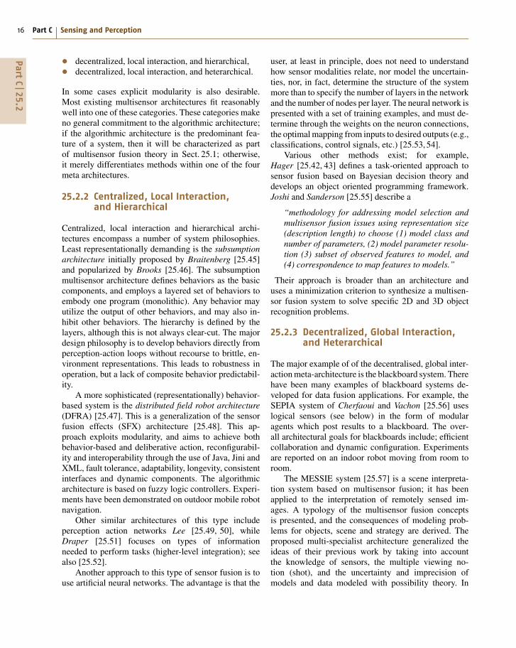
25.2.2 Centralized, Local Interaction,and Hierarchical
Centralized, local interaction and hierarchical archi-tectures encompass a number of system philosophies.Least representationally demanding is the subsumptionarchitecture initially proposed by Braitenberg [25.45]and popularized by Brooks [25.46]. The subsumptionmultisensor architecture defines behaviors as the basiccomponents, and employs a layered set of behaviors toembody one program (monolithic). Any behavior mayutilize the output of other behaviors, and may also in-hibit other behaviors. The hierarchy is defined by thelayers, although this is not always clear-cut. The majordesign philosophy is to develop behaviors directly fromperception-action loops without recourse to brittle, en-vironment representations. This leads to robustness inoperation, but a lack of composite behavior predictabil-ity.
A more sophisticated (representationally) behavior-based system is the distributed field robot architecture(DFRA) [25.47]. This is a generalization of the sensorfusion effects (SFX) architecture [25.48]. This ap-proach exploits modularity, and aims to achieve bothbehavior-based and deliberative action, reconfigurabil-ity and interoperability through the use of Java, Jini andXML, fault tolerance, adaptability, longevity, consistentinterfaces and dynamic components. The algorithmicarchitecture is based on fuzzy logic controllers. Experi-ments have been demonstrated on outdoor mobile robotnavigation.
Other similar architectures of this type includeperception action networks Lee [25.49, 50], whileDraper [25.51] focuses on types of informationneeded to perform tasks (higher-level integration); seealso [25.52].
Another approach to this type of sensor fusion is touse artificial neural networks. The advantage is that the
user, at least in principle, does not need to understandhow sensor modalities relate, nor model the uncertain-ties, nor, in fact, determine the structure of the systemmore than to specify the number of layers in the networkand the number of nodes per layer. The neural network ispresented with a set of training examples, and must de-termine through the weights on the neuron connections,the optimal mapping from inputs to desired outputs (e.g.,classifications, control signals, etc.) [25.53, 54].
Various other methods exist; for example,Hager [25.42, 43] defines a task-oriented approach tosensor fusion based on Bayesian decision theory anddevelops an object oriented programming framework.Joshi and Sanderson [25.55] describe a
“methodology for addressing model selection andmultisensor fusion issues using representation size(description length) to choose (1) model class andnumber of parameters, (2) model parameter resolu-tion (3) subset of observed features to model, and(4) correspondence to map features to models.”
Their approach is broader than an architecture anduses a minimization criterion to synthesize a multisen-sor fusion system to solve specific 2D and 3D objectrecognition problems.
25.2.3 Decentralized, Global Interaction,and Heterarchical
The major example of of the decentralised, global inter-action meta-architecture is the blackboard system. Therehave been many examples of blackboard systems de-veloped for data fusion applications. For example, theSEPIA system of Cherfaoui and Vachon [25.56] useslogical sensors (see below) in the form of modularagents which post results to a blackboard. The over-all architectural goals for blackboards include; efficientcollaboration and dynamic configuration. Experimentsare reported on an indoor robot moving from room toroom.
The MESSIE system [25.57] is a scene interpreta-tion system based on multisensor fusion; it has beenapplied to the interpretation of remotely sensed im-ages. A typology of the multisensor fusion conceptsis presented, and the consequences of modeling prob-lems for objects, scene and strategy are derived. Theproposed multi-specialist architecture generalized theideas of their previous work by taking into accountthe knowledge of sensors, the multiple viewing no-tion (shot), and the uncertainty and imprecision ofmodels and data modeled with possibility theory. In
PartC
25.2
Multisensor Data Fusion 25.2 Multisensor Fusion Architectures 17
particular, generic models of objects are representedby concepts independent of sensors (geometry, mater-ials, and spatial context). Three kinds of specialistsare present in the architecture: generic specialists(scene and conflict), semantic object specialists, andlow level specialists. A blackboard structure witha centralized control is used. The interpreted sceneis implemented as a matrix of pointers enabling con-flicts to be detected very easily. Under the controlof the scene specialist, the conflict specialist resolvesconflicts using the spatial context knowledge of ob-jects. Finally, an interpretation system with SAR/SPOTsensors is described, and an example of a session con-cerned with bridge, urban area and road detection isshown.
25.2.4 Decentralized, Local Interaction,and Hierarchical
One of the earliest proposals for this type of archi-tecture is the RCS (realtime control system) [25.58].RCS is presented as a cognitive architecture for intel-ligent control, but essentially uses multisensor fusionto achieve complex control. RCS focuses on taskdecomposition as the fundamental organizing princi-ple. It defines a set of nodes, each comprised ofa sensor processor, a world model, and a behav-ior generation component. Nodes communicate withother nodes, generally in a hierarchical manner, al-though across layer connections are allowed. The systemsupports a wide variety of algorithmic architectures,from reactive behavior to semantic networks. More-over, it maintains signals, images, and maps, andallows tight coupling between iconic and symbolicrepresentations. The architecture does not generally al-low dynamic reconfiguration, but maintains the staticmodule connectivity structure of the specification.RCS has been demonstrated in unmanned groundvehicles [25.59]. Other object-oriented approaches in-clude [25.34, 60].
An early architectural approach which advocatedstrong programming semantics for multisensor systemsis the logical sensor system (LSS). This approach ex-ploits functional (or applicative) language theory toachieve that.
The most developed version of LSS is instrumentedLSS [25.22]. The ILLS approach is based on LSS in-troduced by Shilcrat and Henderson [25.61]. The LSSmethodology is designed to specify any sensor in sucha way that hides its physical nature. The main goalbehind LSS was to develop a coherent and efficient pre-
sentation of the information provided by many sensors ofdifferent types. This representation provides a means forrecovery from sensor failure, and also facilitates recon-figuration of the sensor system when adding or replacingsensors [25.62].
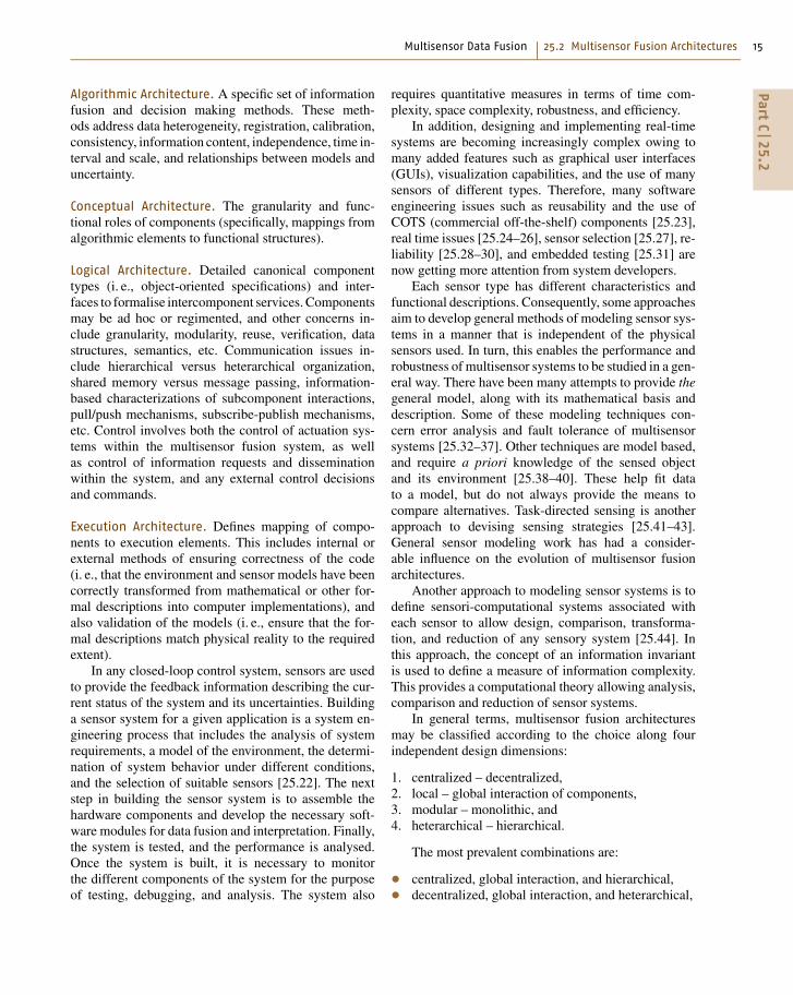
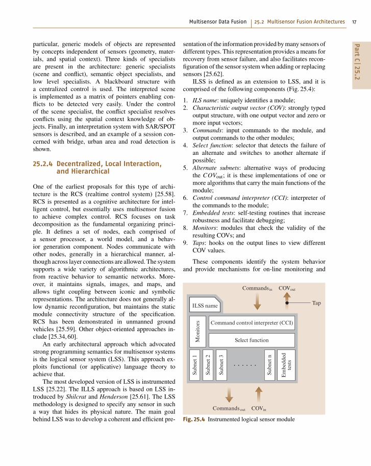
ILSS is defined as an extension to LSS, and it iscomprised of the following components (Fig. 25.4):
1. ILS name: uniquely identifies a module;2. Characteristic output vector (COV): strongly typed
output structure, with one output vector and zero ormore input vectors;
3. Commands: input commands to the module, andoutput commands to the other modules;
4. Select function: selector that detects the failure ofan alternate and switches to another alternate ifpossible;
5. Alternate subnets: alternative ways of producingthe COVout; it is these implementations of one ormore algorithms that carry the main functions of themodule;
6. Control command interpreter (CCI): interpreter ofthe commands to the module;
7. Embedded tests: self-testing routines that increaserobustness and facilitate debugging;
8. Monitors: modules that check the validity of theresulting COVs; and
9. Taps: hooks on the output lines to view differentCOV values.
These components identify the system behaviorand provide mechanisms for on-line monitoring and
Commands out COVin
Commandsin
Command control interpreter (CCI)
Select function
. . . . . .
Mon
itor
sSu
bnet
1
ILSS name
COVout
Tap
Subn
et 2
Subn
et 3
Subn
et n
Em
bedd
edte
sts
Fig. 25.4 Instrumented logical sensor module
PartC
25.2

18 Part C Sensing and Perception
debugging. In addition, they provide handles for mea-suring the run-time performance of the system. Monitorsare validity check stations that filter the output andalert the user to any undesired results. Each moni-tor is equipped with a set of rules (or constraints)that governs the behavior of the COV under differentconditions.
Embedded testing is used for on-line checkingand debugging purposes. Weller proposed a sensor-processing model with the ability to detect measurementerrors and to recover from these errors [25.31]. Thismethod is based on providing each system module withverification tests to verify certain characteristics in themeasured data, and to verify the internal and output dataresulting from the sensor-module algorithm. The recov-ery strategy is based on rules that are local to the differentsensor modules. ILSS uses a similar approach called lo-cal embedded testing, in which each module is equippedwith a set of tests based on the semantic definition ofthat module. These tests generate input data to checkdifferent aspects of the module, then examine the outputof the module using a set of constraints and rules de-fined by the semantics. Also, these tests can take inputfrom other modules to check the operation of a group ofmodules. Examples are given of a wall-pose estimationsystem comprised of a Labmate platform with a cam-era and sonars. Many extensions have been proposed forLSS [25.63, 64].
25.2.5 Decentralized, Local Interaction,and Heterarchical
The best example of this meta architecture is the activesensor network (ASN) framework for distributed datafusion developed by Makarenko [25.21,65]. The distin-guishing features of the various architectures are nowdescribed.
Table 25.1 Canonical components and the roles they play. Multiple X’s in the same row indicate that some inter-rolerelationships are internalized within a component. FRAME does not participate in information fusion or decision makingbut is required for localization and other platform-sepcific tasks (from [25.21])
Component Belief Plan ActionType Source Fuse/Dist Sink Source Fuse/Dist Sink Source Sink
Sensor ×
Node × ×
Actuator ×
Planner × × ×
UI × × ×
Frame
Meta ArchitectureThe distinguishing features of ASN are its commitmentto decentralization, modularity, and strictly local inter-actions (this may be physical or by type). Thus, theseare communicating processes. By decentralized is meantthat no component is central to operation of the sys-tem, and the communication is peer to peer. Also, thereare no central facilities or services (e.g., for commu-nication, name and service lookup or timing). Thesefeatures lead to a system that is scalable, fault tolerant,and reconfigurable.
Local interactions mean that the number of com-munication links does not change with the networksize. Moreover, the number of messages should alsoremain constant. This makes the system scalable andreconfigurable as well.
Modularity leads to interoperability derived from in-terface protocols, reconfigurability, and fault tolerance:failure may be confined to individual modules.
Algorithmic ArchitectureThere are three main algorithmic components: belieffusion, utility fusion and policy selection. Belief fusionis achieved by communicating all beliefs to neighboringplatforms. A belief is defined as a probability distributionof the world state space.
Utility fusion is handled by separating the individualplatform’s partial utility into the team utility of beliefquality and local utilities of action and communication.The downside is that the potential coupling betweenindividual actions and messages is ignored because theutilities of action and communication remain local.
The communication and action policies are chosenby maximizing expected values. The selected approachis to achieve point maximization for one particularstate and follows the work of Manyika and Grochol-sky [25.11, 66].
PartC
25.2
Multisensor Data Fusion 25.3 Applications 19
Conceptual ArchitectureThe data types of the system include
1. beliefs: current world beliefs,2. plans: future planned world beliefs, and3. actions: future planned actions.
The definition of component roles leads to a naturalpartition of the system.
The information fusion task is achieved through thedefinition of four component roles for each data type;these are: source, sink, fuser, and distributor. (Note thatthe data type action does not have fuser or distributorcomponent roles.)
Connections between distributors form the backboneof the ASN framework, and the information exchangedis in the form of their local beliefs. Similar consider-ations are used to determine component roles for thedecision making and the system configuration tasks.
Logical ArchitectureA detailed architecture specification is determinedfrom the conceptual architecture. It is comprised of
six canonical component types as described in Ta-ble 25.1 [25.21].
Makarenko then describes how to combine the com-ponents and interfaces to realize the use cases of theproblem domain in ASN.
Execution ArchitectureThe execution architecture traces the mapping of logi-cal components to runtime elements, such as processesand shared libraries. The deployment view shows themapping of physical components onto the nodes ofthe physical system. The source code view explainshow the software implementing the system is or-ganized. At the architectural level, three items areaddressed: execution, deployment, and source code or-ganization.
The experimental implementation of the ASN frame-work has proven to be flexible enough to accommodatea variety of system topologies, platform and sensorhardware, and environment representations. Several ex-amples are given with a variety of sensors, processorsand hardware platforms.
25.3 Applications
Multisensor fusion systems have been applied to a widevariety of problems in robotics (see references for thischapter), but the two most general areas are dynamicsystem control and environment modeling. Althoughthere is some overlap in these, they may be generallycharacterized as
• dynamic system control: the problem is to use ap-propriate models and sensors to control the stateof a dynamic system (e.g., industrial robot, mo-bile robot, autonomous vehicle, surgical robot, etc.).Usually such systems involve real-time feedbackcontrol loops for steering, acceleration, and behaviorselection. In addition to state estimation, uncer-tainty models are required. Sensors may include,force/torque sensors, gyros, GPS, position encoders,cameras, range finders, etc.;• environment modeling: the problem is to use appro-priate sensors to construct a model of some aspectof the physical environment. This may be a partic-ular object, e.g., a cup, a physical part, a face, etc.,or a larger part of the surroundings: e.g., the interiorof a building, part of a city or an extended remote orunderground area. Typical sensors include cameras,radar, 3-D range finders, IR, tactile sensors and touch
probes (CMMs), etc. The result is usually expressedas geometry (points, lines, surfaces), features (holes,sinks, corners, etc.), or physical properties. Part ofthe problem includes the determination of optimalsensor placement.
25.3.1 Dynamic System Control
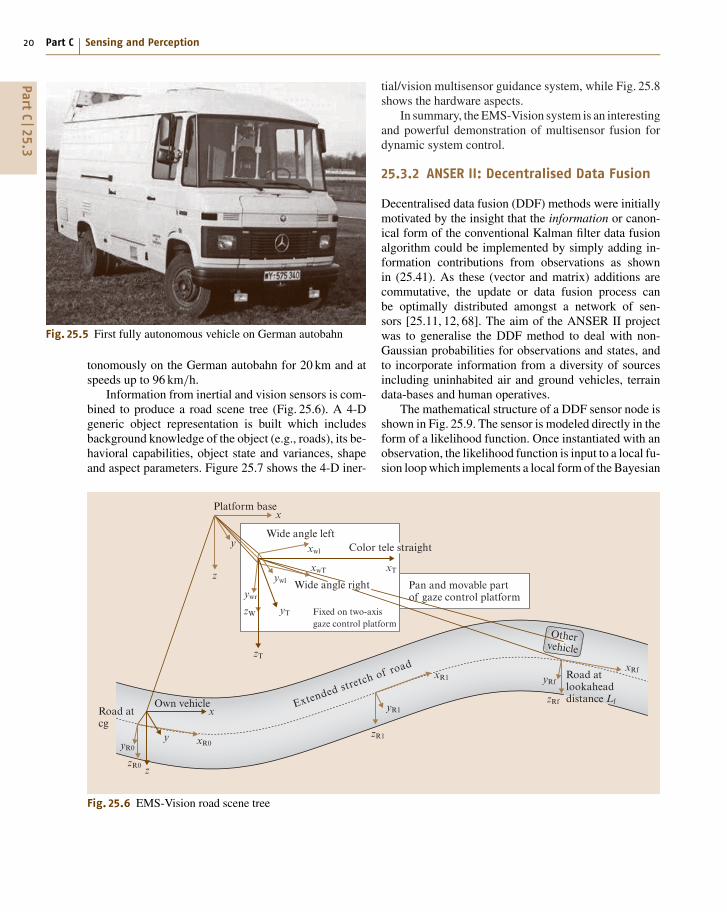
The EMS-Vision system [25.67] is an outstanding ex-emplar of this application domain. The goal is to developa robust and reliable perceptual system for autonomousvehicles. The development goals as stated by the EMS-Vision team are:
• COTS components,• wide variety of objects modeled and incorporatedinto behaviors,• inertial sensors for ego-state estimation,• peripheral/foveal/saccadic vision,• knowledge and goal driven behavior,• state tracking for objects,• 25 Hz real-time update rate.
The approach has been in development since the 1980s;Fig. 25.5 shows the first vehicle to drive fully au-
PartC
25.3
20 Part C Sensing and Perception
Fig. 25.5 First fully autonomous vehicle on German autobahn
tonomously on the German autobahn for 20 km and atspeeds up to 96 km/h.
Information from inertial and vision sensors is com-bined to produce a road scene tree (Fig. 25.6). A 4-Dgeneric object representation is built which includesbackground knowledge of the object (e.g., roads), its be-havioral capabilities, object state and variances, shapeand aspect parameters. Figure 25.7 shows the 4-D iner-
Othervehicle
Wide angle right
Road atcg
Own vehicle
Platform base
Wide angle left
Pan and movable partof gaze control platform
Road atlookaheaddistance Lf
Fixed on two-axisgaze control platform
Extended stretch of roadxR1
xR0yR0
zR0
yR1
zR1
xRf
yRf
zRf
xwl
xTxwTywl
yT
ywr
zT
x
y
z
zW
z
x
y Color tele straight
Fig. 25.6 EMS-Vision road scene tree
tial/vision multisensor guidance system, while Fig. 25.8shows the hardware aspects.
In summary, the EMS-Vision system is an interestingand powerful demonstration of multisensor fusion fordynamic system control.
25.3.2 ANSER II: Decentralised Data Fusion
Decentralised data fusion (DDF) methods were initiallymotivated by the insight that the information or canon-ical form of the conventional Kalman filter data fusionalgorithm could be implemented by simply adding in-formation contributions from observations as shownin (25.41). As these (vector and matrix) additions arecommutative, the update or data fusion process canbe optimally distributed amongst a network of sen-sors [25.11, 12, 68]. The aim of the ANSER II projectwas to generalise the DDF method to deal with non-Gaussian probabilities for observations and states, andto incorporate information from a diversity of sourcesincluding uninhabited air and ground vehicles, terraindata-bases and human operatives.
The mathematical structure of a DDF sensor node isshown in Fig. 25.9. The sensor is modeled directly in theform of a likelihood function. Once instantiated with anobservation, the likelihood function is input to a local fu-sion loop which implements a local form of the Bayesian
PartC
25.3
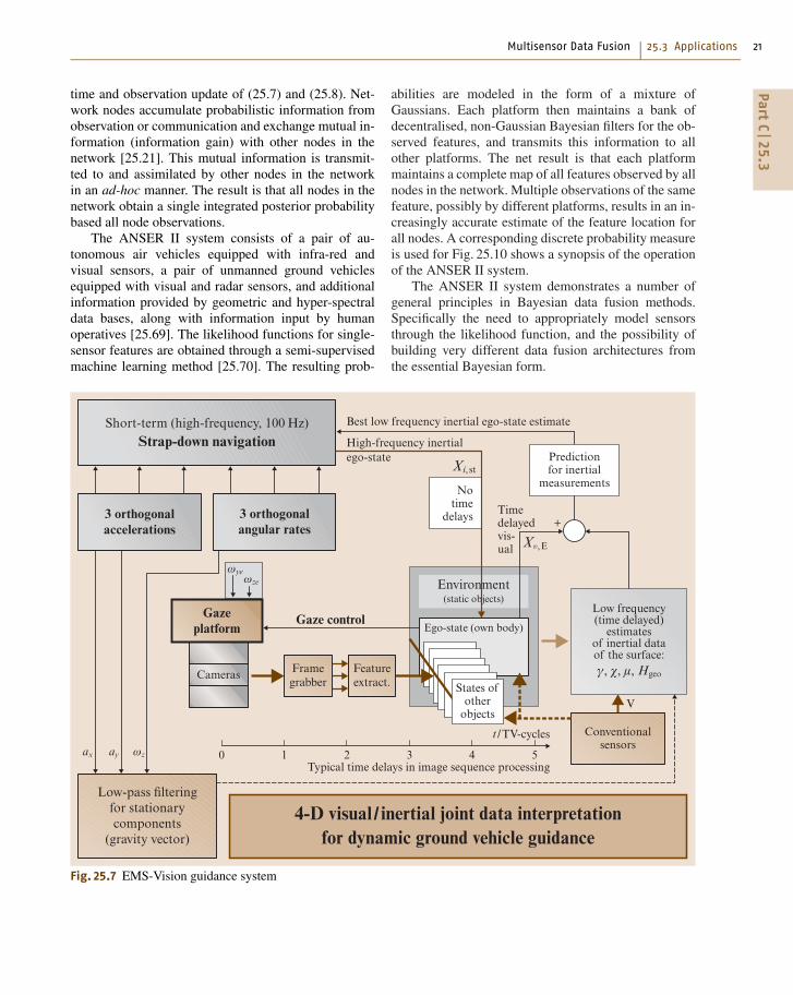
Multisensor Data Fusion 25.3 Applications 21
time and observation update of (25.7) and (25.8). Net-work nodes accumulate probabilistic information fromobservation or communication and exchange mutual in-formation (information gain) with other nodes in thenetwork [25.21]. This mutual information is transmit-ted to and assimilated by other nodes in the networkin an ad-hoc manner. The result is that all nodes in thenetwork obtain a single integrated posterior probabilitybased all node observations.
The ANSER II system consists of a pair of au-tonomous air vehicles equipped with infra-red andvisual sensors, a pair of unmanned ground vehiclesequipped with visual and radar sensors, and additionalinformation provided by geometric and hyper-spectraldata bases, along with information input by humanoperatives [25.69]. The likelihood functions for single-sensor features are obtained through a semi-supervisedmachine learning method [25.70]. The resulting prob-
Best low frequency inertial ego-state estimate
t /TV-cycles
Typical time delays in image sequence processing
Timedelayedvis-ual
+
Notime
delays
Short-term (high-frequency, 100 Hz)Strap-down navigation
4-D visual / inertial joint data interpretationfor dynamic ground vehicle guidance
Xi, st
Xυ,E
High-frequency inertialego-state
Gaze controlGazeplatform
3 orthogonalangular rates
Framegrabber
0 1 2 3 4 5
V
Cameras Featureextract.
Ego-state (own body)
Conventionalsensors
Environment
γ, �, μ, Hgeo
Low frequency(time delayed)
estimatesof inertial dataof the surface:
(static objects)
ωyeωze
ωzayax
3 orthogonalaccelerations
Low-pass filteringfor stationarycomponents
(gravity vector)
States ofother
objects
Predictionfor inertial
measurements
Fig. 25.7 EMS-Vision guidance system
abilities are modeled in the form of a mixture ofGaussians. Each platform then maintains a bank ofdecentralised, non-Gaussian Bayesian filters for the ob-served features, and transmits this information to allother platforms. The net result is that each platformmaintains a complete map of all features observed by allnodes in the network. Multiple observations of the samefeature, possibly by different platforms, results in an in-creasingly accurate estimate of the feature location forall nodes. A corresponding discrete probability measureis used for Fig. 25.10 shows a synopsis of the operationof the ANSER II system.
The ANSER II system demonstrates a number ofgeneral principles in Bayesian data fusion methods.Specifically the need to appropriately model sensorsthrough the likelihood function, and the possibility ofbuilding very different data fusion architectures fromthe essential Bayesian form.
PartC
25.3
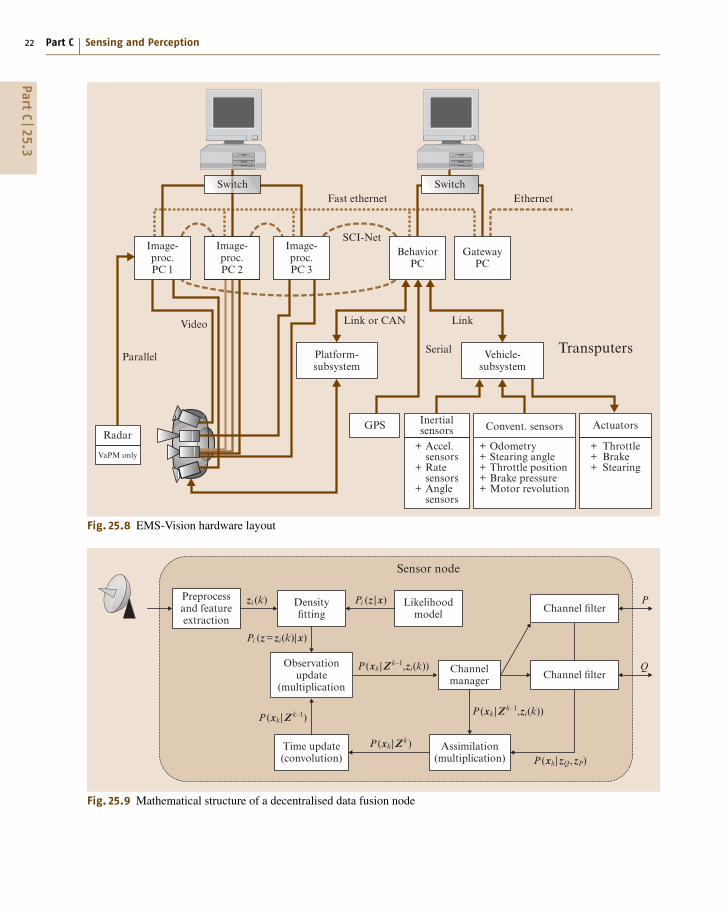
22 Part C Sensing and Perception
Fast ethernetSwitch Switch
Radar
Parallel
Video
VaPM only
Image-proc.PC 2
SCI-Net
Link or CAN
+ Accel. sensors+ Rate sensors+ Angle sensors
+ Odometry+ Stearing angle+ Throttle position+ Brake pressure+ Motor revolution
Link
Serial Transputers
Image-proc.PC 1
Image-proc.PC 3
Platform-subsystem
Vehicle-subsystem
Inertialsensors
+ Throttle+ Brake+ Stearing
ActuatorsConvent. sensorsGPS
Ethernet
BehaviorPC
GatewayPC
Fig. 25.8 EMS-Vision hardware layout
Densityfitting
Likelihoodmodel
Time update(convolution)
Assimilation(multiplication)
Sensor node
zi (k) Pi (z |x)
P (xk |Zk–1,zi(k))
P (xk |Zk–1,zi(k))
P (xk |zQ,zP)
P (xk |Zk–1)
P (xk |Zk)
Pi (z=zi(k)|x)
Channel filterP
Channel filterChannelmanager
Q
Preprocessand featureextraction
Observationupdate
(multiplication
Fig. 25.9 Mathematical structure of a decentralised data fusion node
PartC
25.3
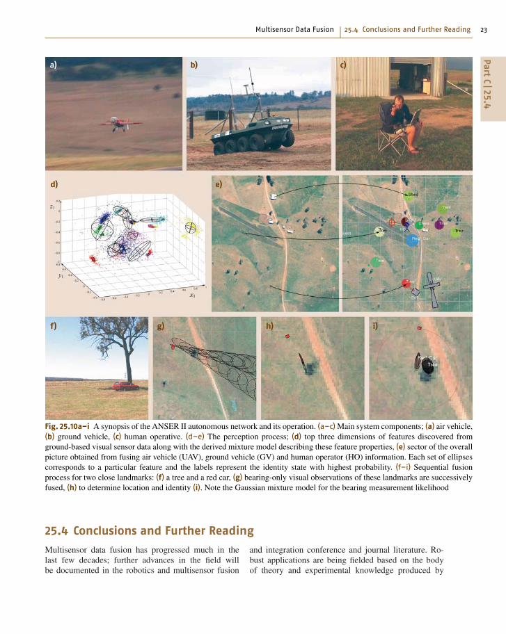
Multisensor Data Fusion 25.4 Conclusions and Further Reading 23
Fig. 25.10a–i A synopsis of the ANSER II autonomous network and its operation. (a–c) Main system components; (a) air vehicle,(b) ground vehicle, (c) human operative. (d–e) The perception process; (d) top three dimensions of features discovered fromground-based visual sensor data along with the derived mixture model describing these feature properties, (e) sector of the overallpicture obtained from fusing air vehicle (UAV), ground vehicle (GV) and human operator (HO) information. Each set of ellipsescorresponds to a particular feature and the labels represent the identity state with highest probability. (f–i) Sequential fusionprocess for two close landmarks: (f) a tree and a red car, (g) bearing-only visual observations of these landmarks are successivelyfused, (h) to determine location and identity (i). Note the Gaussian mixture model for the bearing measurement likelihood
25.4 Conclusions and Further Reading
Multisensor data fusion has progressed much in thelast few decades; further advances in the field willbe documented in the robotics and multisensor fusion
and integration conference and journal literature. Ro-bust applications are being fielded based on the bodyof theory and experimental knowledge produced by
PartC
25.4
24 Part C Sensing and Perception
the research community. Current directions of interestinclude:
1. large-scale, ubiquitous sensor systems,2. bio-based or biomimetic systems,3. medical in situ applications, and4. wireless sensor networks.
Representative large-scale examples include intelligentvehicle and road systems, as well as instrumentedcontexts such as cities. Biological principles mayprovide fundamentally distinct approaches to the ex-ploitation of dense, redundant, correlated, noisy sensors,especially when considered as part of a Gibbsianframework for behavioral response to environmen-tal stimuli. Another issue here is the developmentof a theoretical understanding of sensor system de-velopment, adaptivity and learning with respect to
the particular context in which the system is de-ployed.
Further pushing the envelope of both technology andtheory will permit the introduction of micro and nanosensors into the human body and allow the monitor-ing and locally adaptive treatment of various maladies.Finally, a more complete theoretical framework is stillrequired which encompasses system models for wire-less sensor networks. This should include models of thephysical phenomena being monitored, as well as opera-tional and network issues. Finally, numerical analysis ofthe algorithmic properties of data-driven systems withsensor data error sources which must be unified with theanalysis of truncation, roundoff, and other errors.
A firm foundation exists upon which to build thesenew theories, systems, and applications. It will be a vi-brant area of research for years to come!
References
25.1 S. Thrun, W. Burgard, D. Fox: Probabilistic Robotics(MIT Press, Cambridge 2005)
25.2 J.O. Berger: Statistical Decision Theory andBayesian Analysis (Springer, Berlin, Heidelberg
1985)
25.3 A. Elfes: Sonar-based real-world mapping and
navigation, IEEE Trans. Robot. Autom. 3(3), 249–265
(1987)
25.4 A. Elfes: Integration of sonar and stereo range data
using a grid-based representation, Proc. IEEE Int.
Conf. Robot. Autom. (1988) 727–
25.5 L.D. Stone, C.A. Barlow, T.L. Corwin: Bayesian Mul-tiple Target Tracking (Artech House, Norwood 1999)
25.6 Y. Bar-Shalom: Multi-Target Multi-Sensor Tracking(Artec House, Norwood 1990)
25.7 Y. Bar-Shalom, T.E. Fortmann: Tracking and DataAssociation (Academic, New York 1988)
25.8 P.S. Maybeck: Stochastic Models, Estimaton andControl, Vol. I (Academic, New York 1979)
25.9 W. Sorensen: Special issue on the applications of
the Kalman filter, IEEE Trans. Autom. Control 28(3),
(1983)
25.10 B.D.O. Anderson, J.B. Moore: Optimal Filtering(Prentice Hall, Upper Saddle River 1979)
25.11 J. Manyika, H.F. Durrant-Whyte: Data Fusion andSensor Management: An Information-TheoreticApproach (Prentice Hall, Upper Saddle River
1994)
25.12 S. Sukkarieh, E. Nettleton, J.H. Kim, M. Ridley,
A. Goktogan, H. Durrant-Whyte: The ANSER project:
Data fusion across multiple uninhabited air vehi-
cles, Int. J. Robot. Res. 22(7), 505–539 (2003)
25.13 R.E. Moore: Interval Analysis (Prentice Hall, Upper
Saddle River 1966)
25.14 D. Dubois, H. Prade: Fuzzy Sets and Systems: Theoryand Applications (Academic, New York 1980)
25.15 S. Blackman, R. Popoli: Design and Analysis ofModern Tracking Systems (Artec House, Norwood
1999)
25.16 D. Pagac, E.M. Nebot, H. Durrant-Whyte: An evi-
dential approach to map-building for autonomous
vehicles, IEEE Trans. Robot. Autom. 14(4), 623–629
(1998)
25.17 D. Hall, J. Llinas: Handbook of Multisensor DataFusion (CRC, Boca Raton 2001)
25.18 E.L. Waltz, J. Llinas: Sensor Fusion (Artec House,
Norwood 1991)
25.19 M. Kam, Z. Zhu, P. Kalata: Sensor fusion for mobile
robot navigation, IEEE Proc. 85, 108–119 (1997)
25.20 H. Carvalho, W. Heinzelman, A. Murphy, C. Coelho:
A general data fusion architecture, Proc. 6th Int.
Conf. Inf. Fusion, Cairns (2003)
25.21 A. Makarenko: A Decentralized Architecture for Ac-
tive Sensor Networks. Ph.D. Thesis (University of
Sydney, Sydney 2004)
25.22 M. Dekhil, T. Henderson: Instrumented logical sen-
sors systems, Int. J. Robot. Res. 17(4), 402–417
(1998)
25.23 J.A. Profeta: Safety-critical systems built with COTS,
IEEE Comput. 29(11), 54–60 (1996)
25.24 H. Hu, J.M. Brady, F. Du, P. Probert: Distributed
real-time control of a mobile robot, J. Intell. Au-
tom. Soft Comput. 1(1), 63–83 (1995)
25.25 S.A. Schneider, V. Chen, G. Pardo: ControlShell: A
real-time software framework, AIAA Conf. Intell.
Robot. Field Fact. Serv. Space (1994)
25.26 D. Simon, B. Espiau, E. Castillo, K. Kapellos:
Computer-aided design of a generic robot con-
PartC
25
Multisensor Data Fusion References 25
troller handling reactivity and real-time issues,
IEEE Trans. Control Syst. Technol. 4(1), (1993)
25.27 C. Giraud, B. Jouvencel: Sensor selection in a fu-
sion process: a fuzzy approach, Proc. IEEE Int. Conf.
Multisens. Fusion Integr., Las Vegas (1994) 599–606
25.28 R. Kapur, T.W. Williams, E.F. Miller: System testing
and reliability techniques for avoiding failure, IEEE
Comput. 29(11), 28–30 (1996)
25.29 K.H. Kim, C. Subbaraman: Fault-tolerant real-time
objects, Commun. ACM 40(1), 75–82 (1997)
25.30 D.B. Stewart, P.K. Khosla: Mechanisms for detect-
ing and handling timing errors, Commun. ACM
40(1), 87–93 (1997)
25.31 G. Weller, F. Groen, L. Hertzberger: A sensor
processing model incorporating error detection
and recovery. In: Traditional and Non-TraditionalRobotic Sensors, ed. by T. Henderson (Springer,
Berlin, Heidelberg 1990) pp. 351–363
25.32 R.R. Brooks, S. Iyengar: Averaging algorithmfor multi-dimensional redundant sensor ar-rays: resolving sensor inconsistencies, Tech. Rep.
(Louisiana State University, 1993)
25.33 T.C. Henderson, M. Dekhil: Visual target based wallpose estimation, Tech. Rep. UUCS-97-010 (Univer-
sity of Utah, 1997)
25.34 S. Iyengar, D. Jayasimha, D. Nadig: A versatile ar-
chitecture for the distributed sensor integration
problem, IEEE Comput. 43, 175–185 (1994)
25.35 D. Nadig, S. Iyengar, D. Jayasimha: New archi-
tecture for distributed sensor integration, IEEE
SOUTHEASTCON Proc. (1993)
25.36 L. Prasad, S. Iyengar, R.L. Kashyap, R.N. Madan:
Functional characterization of fault tolerant inte-
gration in distributed sensor networks, IEEE Trans.
Syst. Man Cybern. , 1082–1087 (1991)
25.37 L. Prasad, S. Iyengar, R. Rao, R. Kashyap: Fault-
tolerence sensor integration using multiresolution
decomposition, Am. Phys. Soc. , 3452–3461 (1994)
25.38 H.F. Durrant-Whyte: Integration, Coordination,and Control of Multi-Sensor Robot Systems (Kluwer
Academic, Boston 1987)
25.39 F. Groen, P. Antonissen, G. Weller: Model based
robot vision, IEEE Instrum. Meas. Technol. Conf.
(1993) 584–588
25.40 R. Joshi, A.C. Sanderson: Model-based multisensor
data fusion: a minimal representation approach,
Proc. IEEE Int. Conf. Robot. Autom. (1994)
25.41 A.J. Briggs, B.R. Donald: Automatic sensor config-
uration for task-directed planning, Proc. IEEE Int.
Conf. Robot. Autom. (1994) 1345–1350
25.42 G. Hager: Task Directed Sensor Fusion and Planning(Kluwer Academic, Boston 1990)
25.43 G. Hager, M. Mintz: Computational methods for
task-directed sensor data fusion and sensor plan-
ning, Int. J. Robot. Res. 10(4), 285–313 (1991)
25.44 B. Donald: On information invariants in robotics,
Artif. Intell. 72, 217–304 (1995)
25.45 V. Braitenberg: Vehicles: Experiments in SyntheticPsychology (MIT Press, Cambridge 1984)
25.46 R.A. Brooks: A robust layered control system for a
mobile robot, IEEE Trans. Robot. Autom. 2(1), 14–23
(1986)
25.47 K.P. Valavanis, A.L. Nelson, L. Doitsidis, M. Long,
R.R. Murphy: Validation of a distributed field robot
architecture integrated with a matlab based con-
trol theoretic environment: A case study of fuzzy
logic based robot navigation, CRASAR 25 (University
of South Florida, 2004)
25.48 R.R. Murphy: Introduction to AI Robotics (MIT Press,
Cambridge 2000)
25.49 S. Lee: Sensor fusion and planning with
perception-action network, Proc. IEEE Conf. Mul-
tisens. Fusion Integr. Intell. Syst., Washington
(1996)
25.50 S. Lee, S. Ro: Uncertainty self-management with
perception net based geometric data fusion, Proc.
IEEE Conf. Robot. Autom., Albuquerque (1997)
25.51 B.A. Draper, A.R. Hanson, S. Buluswar, E.M. Rise-
man: Information acquisition and fusion in the
mobile perception laboratory, Proc. SPIE – Signal
Processing, Sensor Fusion, and Target Recognition
VI, Vol. 2059 (1996) 175–187
25.52 S.S. Shafer, A. Stentz, C.E. Thorpe: An architecture
for sensor fusion in a mobile robot, Proc. IEEE Int.
Conf. Robot. Autom. (1986) 2002–2007
25.53 S. Nagata, M. Sekiguchi, K. Asakawa: Mobile robot
control by a structured hierarchical neural net-
work, IEEE Control Syst. Mag. 10(3), 69–76 (1990)
25.54 M. Pachter, P. Chandler: Challenges of autonomous
control, IEEE Control Syst. Mag. 18(4), 92–97 (1998)
25.55 R. Joshi, A.C. Sanderson: Multisensor Fusion (World
Scientific, Singapore 1999)
25.56 V. Berge-Cherfaoui, B. Vachon: Dynamic configu-
ration of mobile robot perceptual system, Proc. IEEE
Conference on Multisensor Fusion and Integration
for Intelligent Systems, Las Vegas (1994)
25.57 V. Clement, G. Giraudon, S. Houzelle, F. Sandakly:
Interpretation of remotely sensed images in a con-
text of mulrisensor fusion using a multi-specialist
architecture, Rapport de Recherche: Programme 4
- Robotique, Image et Vision 1768, INRIA (1992)
25.58 J. Albus: RCS: A cognitive architecture for intelli-
gent multi-agent systems, Proc. IFAC Symp. Intell.
Auton. Veh., Lisbon (2004)
25.59 R. Camden, B. Bodt, S. Schipani, J. Bornstein,
R. Phelps, T. Runyon, F. French: Autonomousmobility technology assessment: Interim report,ARL-MR 565 (Army Research Laboratory, 2003)
25.60 T. Queeney, E. Woods: A generic architecture for
real-time multisensor fusion tracking algorithm
development and evaluation, Proc. SPIE – Signal
Processing, Sensor Fusion, and Target Recognition
VII, Vol. 2355 (1994) 33–42
25.61 T. Henderson, E. Shilcrat: Logical sensor systems, J.
Robot. Syst. , 169–193 (1984)
PartC
25
26 Part C Sensing and Perception
25.62 T. Henderson, C. Hansen, B. Bhanu: The specifica-
tion of distributed sensing and control, J. Robot.
Syst. , 387–396 (1985)
25.63 J.D. Elliott: Multisensor fusion within an encap-
sulated logical device architecture. Master’s Thesis
(University of Waterloo, Waterloo 2001)
25.64 M.D. Naish: Elsa: An intelligent multisensor inte-
gration architecture for industrial grading tasks.
Master’s thesis (University of Western Ontario, Lon-
don 1998)
25.65 A. Makarenko, A. Brooks, S. Williams, H. Durrant-
Whyte, B. Grocholsky: A decentralized architecture
for active sensor networks, Proc. IEEE Int. Conf.
Robot. Autom., New Orleans (2004) 1097–1102
25.66 B. Grocholsky, A. Makarenko, H. Durrant-Whyte:
Information-theoretic coordinated control of mul-
tiple sensor platforms, Proc. IEEE Int. Conf. Robot.
Autom., Taipei (2003) 1521–1527
25.67 R. Gregor, M. Lützeler, M. Pellkofer, K.-H. Sieder-
sberger, E. Dickmanns: EMS-Vision: A perceptual
system for autonomous vehicles, IEEE Trans. Intell.
Transp. Syst. 3(1), (2002)
25.68 B. Rao, H. Durrant-Whyte, A. Sheen: A fully de-
centralized multi-sensor system for tracking and
surveillance, Int. J. Robot. Res. 12(1), 20–44 (1993)
25.69 B. Upcroft: Non-gaussian state estimation in an
outdoor decentralised sensor network, Proc. IEEE
Conf. Decis. Control (CDC) (2006)
25.70 S. Kumar, F. Ramos, B. Upcroft, H. Durrant-Whyte:
A statistical framework for natural feature repre-
sentation, Proc. IEEE/RSJ Int. Conf. Intell. Robot.
Syst. (IROS), Edmonton (2005) 1–6
PartC
25

http://www.springer.com/978-3-540-23957-4