Multipolar continuum mechanics - University of …maeresearch.ucsd.edu/goddard/Pisa/Lecture01/Reprints/green64b.pdfMultipolar Continuum Mechanics t I 5 For some purposes it is convenient

Multipolar Continuum Mechanics A. E. GREEN & R. S. RIVLIN

Abstract A general t h e o r y of mu l t ipo la r d i sp lacement and ve loc i ty fields wi th cor-

responding mul t ipo la r b o d y and surface forces and mul t ipo la r stresses is deve loped using an energy principle, an e n t r o p y p roduc t ion i ne qua l i t y and in- va r iance condi t ions under superposed r ig id b o d y motions. Cons t i tu t ive equat ions for the mul t ipo la r stresses are discussed and expl ic i t resul ts are given for an e las t ic medium. W o r k in a previous pape r b y the presen t au thors (t964) is shown to be a special case of t h a t given here.

Contents Page 1. In t roduct ion . . . . . . . . . . . . . . . . . . . . . . . . . . . . 1 t 3 2. Monopolar kinematics . . . . . . . . . . . . . . . . . . . . . . . . 114 3. Superposed r igid-body motions . . . . . . . . . . . . . . . . . . . . t t6 4. Multipolar kinematics . . . . . . . . . . . . . . . . . . . . . . . . 1 t 7 5. Multipolar body forces . . . . . . . . . . . . . . . . . . . . . . . . 120 6. Multipolar surface forces and stresses . . . . . . . . . . . . . . . . . t 21 7. Kinet ic energy . . . . . . . . . . . . . . . . . . . . . . . . . . . 123 8. The energy equation and ent ropy production inequal i ty . . . . . . . . . t 23 9. Energy and ent ropy production : a l ternat ive form . . . . . . . . . . . . 126

t0. Elas t ic i ty . . . . . . . . . . . . . . . . . . . . . . . . . . . . . i28 t 1. Elas t ic i ty : a l ternat ive form . . . . . . . . . . . . . . . . . . . . . . 13 t t 2. Consti tutive equations . . . . . . . . . . . . . . . . . . . . . . . . t 33 13. Consti tutive equations: a l ternat ive form . . . . . . . . . . . . . . . . 134 t4. Elas t ic i ty : relation to previous theory . . . . . . . . . . . . . . . . . 136 t 5. Infinitesimal elast ici ty . . . . . . . . . . . . . . . . . . . . . . . . t 38 t6. Equations of motion and variat ional equations . . . . . . . . . . . . . t41 t7. Appendix . . . . . . . . . . . . . . . . . . . . . . . . . . . . . t42 References . . . . . . . . . . . . . . . . . . . . . . . . . . . . . . . 147

1. Introduction

In a previous pape r GREEN & RIVLIN (t964) have deve loped a genera l t heo ry of s imple force and stress mul t ipoles which were def ined wi th the help of ve loc i ty componen t s and the i r spa t i a l der ivat ives . In t h a t pape r we ind ica t ed direc- t ions in which the t heo ry could be general ized. Here we l ay the founda t ions of a t h e o r y of considerable genera l i ty which includes the work of the previous p a p e r as a special case.

The s t a r t i ng po in t of the presen t inves t iga t ion rests on some ideas of TRuEs- DELL & TOUPIN (1960, sect ions t66, 205, 232). These au thors in t roduced genera l ized velocit ies, b o d y and surface forces, and genera l ized stresses.* T h e y

* Special types of generalized displacement and velocity fields have been used b y ERICKSEN (t960a, 1960b, t960c, 1961).

t t4 A . E . GREEN & R. S. RIVLIN:

postulated equations of motion in terms of generalized stresses and body forces, and they postulated surface conditions. TRUESDELL & TOOPIN alSO discussed a general type of virtual work theorem and showed that it was equivalent to their equations of motion and surface conditions. In the present paper we use, essentially, the same definitions of generalized body and surface forces and stresses as those of TRUESDELL & TOUPIN, but a new condition is imposed on our definition of generalized displacement and velocity. We find that the equations of motion and surface conditions given by TRUESDELL & TOUPIN are not necessarily always satisfied. Sufficient conditions under which these equations are valid are discussed in section 16. The same conditions are then sufficient for the validity of the virtual work equation.

Kinematics of ordinary displacement and velocity fields, now called monopolar kinematics, is briefly reviewed in sections 2, 3. The theory of multipolar displacements and velocities is developed in section 4. Multipolar body forces are defined in section 5, and multipolar surface forces and stresses in section 6. Appropriate expressions for kinetic energy corresponding to multipolar velocities are given in section 7. The fundamental dynamical theory of multipolar forces and stresses is considered in section 8 using only an energy equation, an entropy production inequality, and invariance conditions under superposed rigid body motions. An alternative form for this theory is given in section 9. A general theory of elasticity for multipolar stresses and forces is developed in section t0, with an alternative form in section 1t.

Questions concerning constitutive equations for materials which are not elastic are considered in sections t2, t3. In section t4 we show that the elasticity theory given previously (1964) is a special case of tile theory of elasticity given in section t0. In section 15 we derive the approximate theory of infinitesimal elasticity appropriate to elastic materials acted on by monopolar and dipolar stresses.*

2. Monopolar kinematics

We refer the motion of the continuum to a fixed system of rectangular cartesian axes. The position of a typical particle of the continuum at time is denoted by x i(3) where

x~(~)=x~(X1, x~, x~, "0 ( - ~176 (2.t)

and X a is a reference position of the particle. We also use the notation

X i ~ - x ~ ( t ) . (2.2)

If this deformation is to be possible in a real material then

~, [ axi(~) ] d:~ [ -~7 -a ] > o. (2.3)

* After completing the present paper the authors saw a report by R. D. MINDLIN on "Microstructure in Linear Elasticity" in which he develops a theory which is essentially the same as that contained in w t 5 of our paper. MINDLIN has applied his theory to wave propagation and this application has not been studied here. This paper has now been published in Arch. Rational Mech. Anal. 16, 5t--78 (t964).

Multipolar Continuum Mechanics t I 5

For some purposes it is convenient to express x i (3) in t e rms of the current posit ion of the part icle a t t ime t so t ha t

x ~ ( z ) = x i ( x l , x s, x 3, t, 3) (2.4) and

[ a-,/~/1 det [ ~ : - i ] > 0. (2.5)

Disp lacement gradients t aken with respect to the posit ion X a are denoted b y

~ x i ( r ) (/3 = t , 2 . . . . ), (2.6) xi,a~a .... ap (T) = OXal OXa, ... OXa~

and we use the no ta t ion x~,a . . . . a p = x i , a . . . . ap (t). (2.7)

Displacement gradients t aken with respect to the current position x i a t t ime t are

OOxi(r) (/5 = t , 2 . . . . ). (2.8) Xi, i, i,... 0 (~) - - ~x~ Ox~ . . . . ~xia

We observe t h a t

xi, i, (t) = 0 ii,, (2.9)

xi , i . . . . i , ( t ) = 0 ( / ~ > t ) ,

and t h a t the gradients in (2.7) and (2.8) are symmet r i c with respect to A1, A2, . . . . A a and i 1, i 2 . . . . . ia respect ively.

The components of veloci ty a t the point x i(z) are denoted b y v! x) ( 3 ) = v i(r) so t h a t

v! 1) (~) = D x i (r) /D z , v! x) (t) = v i (0 = vi,

where D[D r denotes different iat ion with respect to r holding X a f ixed in (2A), or xi( t ) and t f ixed in (2.4). More generally, n th veloci ty components m a y be defined as

v! ") (r) = D" x i (z) /D r", v! '0 (t) = v! "), v! ~ (x) = x i (r). (2.t 0)

F r o m (2.8) and (2A0) we have

D" x~,il ... ip (3) ear!-) (T) - = ~!"),... , , (~), (2 .~ t )

D T n 8xil Ore, ... Oxia

and we use the no ta t ion v!"!l . . , , (0 = ~!"! . . . . i , (2 .12)

for gradients of the n tu veloci ty components a t t ime t wi th respect to coordinates a t t ime t. Also

v (~ �9 (r)-----x/, i .... i,(l~), v I~ - - - 0 ( f l > l ) (2A3)

In view of (2.3) we m a y write xi, a (~) in the polar form

Xi, a (3) = R i B (3) MBa (~), (2A4)

where MBa (r) is a posi t ive definite symmet r i c tensor and RiB(r ) is a ro ta t ion tensor, so t h a t

RiB (z) R ia (r) = ~)A B, R ia (T) R ia (z) = ~)ii, det Ri a (3) = t . (2.t 5)

t t 6 A .E . GREEN ~r R. S. RIVLIN:

Also R i B = R i B ( t ) , M A B = M a B ( t ) . (2.t6)

In general, th roughout the paper , lower case Lat in indices i, il . . . . are associated with coordinates xi(3 ) or x i and take the values t , 2, 3; upper case Lat in indices A, A1 . . . . are associated with coordinates X A and t ake the values l , 2, 3. The usual cartesian summat ion convent ion is used, and commas denote par t ia l differentiation.

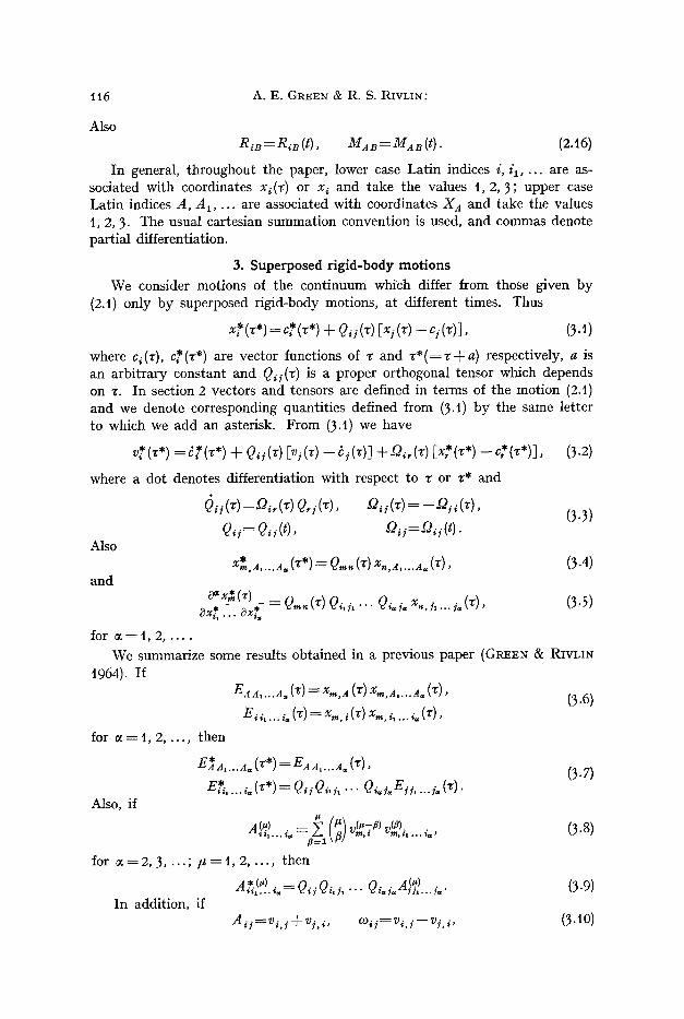
3. Superposed r ig id -body m o t i o n s

We consider mot ions of the con t inuum which differ f rom those given b y (2.t) only b y superposed r igid-body motions, a t different t imes. Thus

x* (3*) = c* (3*) + Q . (3) [xj (3) - c; (~)], (3.1)

where c~(3), c*(z*) are vector functions of z and z * ( = r + a ) respectively, a is an a rb i t r a ry cons tant and Qii(3) is a proper or thogonal tensor which depends on 3. In section 2 vectors and tensors are defined in t e rms of the mot ion (2.t) and we denote corresponding quant i t ies defined f rom (3.1) b y the same let ter to which we add an asterisk. F rom (3.1) we have

v*(3*) =~*(3") + Q,(3) [v;(~) - ~ j ( 3 ) ] +~%,(3) Ix*(3*) - c * ( 3 " ) ] , (3.2)

where a dot denotes differentiat ion with respect to ~ or ~* and

(i~i (~) =~%, (3) Q,j(~), G j ( 3 ) = -Qii(3), (3.3) ( G = Q. ( t ) , G j - - G ; ( t ) .

Also ,~,a .... a . t J - Q , ~ ( * ) x , , a .... A,(3), (3.4)

and ~ x * ( , )

e,i*, ... e~* - Q ~ (~) Qi, i , . . . Qi. j. x,, j .... i~ (~), (3.5)

for ~----1,2 . . . . . We summar ize some results obta ined in a previous paper (GREE~ & RIVLIN

1964). I f E a a .... A . (3) = Xm, A (~) Xm, A . . . . A~ ( ' r ) ,

(3.6) E . .... i . (~)=x~, i (3)x~,~ .... ~.(3),

for 0~ = 1, 2, . . . , then

E * & . . . a . (**) = E A A . . . . A, (Z), (3.7)

E*i . . . . i , (**) = Q i i Q i , h . . . Qi , i, E i i . . . . i, (3). Also, if

/* ACU) _ ~, {a~ vCV-#) yea). (3.8) ii . . . . i~, - - z.~ I r} m,* m, ~ . . . i~,,

.e=l

for a = 2 , 3, . . . ; / , = 1 , 2 . . . . , then

r~ ~l .) (3.9) A * ( ~ ) " = Q i i Q i ~ j ~ 'dio, i ~ , " i J . . . . j,, i i~ . . . ,~ . . . . In addition, if

A i j - ~ ' v i , j + v j , i , r j - - v i , i , (3.10)

Multipolar Continuum Mechanics

then 2 v i , i = A i i +coi i, (3.1 l) and

A*=Q~,,Qi,,A,,, ,~, w*.=qi , ,q i ,~w, , ,~+ 20 i i . (3.12)

4. Mul t ipo la r k i n e m a t i c s

The d isplacement funct ion x i (3) can be regarded either as a funct ion of X a , as in (2.t) or as a funct ion of x i, t, ~ as in (2.4). The form (2.1) is appropr ia te

to cont inua in which a reference posit ion is required and (2.4) is convenient when there is no preferred reference state. We now define a simple 2~-pole d isplacement field in two forms .* Let

x~a .... a n ( ~ ) = x ~ . .... an(X,,X2, X2, 3) (-- oo<~__<t), (4.t)

be a tensor function under changes of rec tangular cartesian axes for fl : t , 2 . . . . . The set of tensors (4.t) is a set of k inemat ic variables which m a y be changed independent ly of the mot ion (2A), but when the mot ion (2.1) is changed these tensors will, in general, be altered. When the mot ion is a l tered f rom (2.t) to (3.t) we denote the corresponding tensor (4.t) b y x*a .... an (3*). If, in addi t ion to the above assumpt ions about the tensor (4A),

x~a,...an(z*)=Q,,,,(r)x,,a,...an(r) (fl-__l), (4.2)

then we m a y say t ha t xla .... an (3) is a simple 2&pole displacement /ield. For example , if

xia .... an (3) = x~,a,...an (~), (4.3)

then the tensor (4.3) satisfies the pos tu la ted conditions. Re turn ing to the general tensor (4.1) we use the no ta t ion

x~a .... an = x i a , . . . n n (t) (4.4) and we observe t h a t the tensor in (4.t) does not necessari ly have symmetr ies in any of its indices.

Again let

x~i . . . . jn(~)=x~; .... in(x1, x~, x3, t, 3) ( - o o < , < t ) (4.5)

be a tensor function for fl = t , 2 . . . . which is such t ha t

x~* i,... i , (3*) = Q,, ~ (3) QA i , - . . Qin in x,, ~,... 0 (3). (4.6)

Then we say t ha t xii .... in (3) is also a simple 2a-pole displacement/ield and we use the nota t ion

xii .... ~'n = xii .... ~'n (t). (4.7)

An example of such a displacement field is

xii .. . . in (3) = x, , i .... in (3). (4.8)

A 2a-pole d isplacement field of the t ype (4.5) can be ob ta ined f rom the field (4.t) in m a n y different ways, and conversely, as indicated in the appendix.

* A possible motivation for the definitions given here is indicated in the Appendix. Arch. Rational Mech. Anal., Vol. 17 9

t t8 A . E . GREEN & 1~. S. RIVLIN:

One simple me thod of relat ing the two fields is b y the equat ion

%i .... ia (T) = x i l ,B , . . . xi a,B axiB .... Ba (T), (4.9)

bu t this m a y not a lways be the re levant relat ion to use. In mos t of this pape r we assume tha t (4.1) and (4.5) are independent descriptions of mul t ipolar dis- p lacement fields.

We define 2a-pole velocity fields f rom the 2a-pole displacements (4.t) or (4.5) b y the equat ions

vi~ .... ~.(~) = ~ .... ~ . (~) , (4 . to)

vi i . . . . i , (T) = ~ i . . . . j, (~), (4.11)

for fl = 1, 2 . . . . . where a dot denotes mate r ia l t ime differentiat ion with respect to z holding X A fixed in (4.10) and t and x i f ixed in (4. t l ) . We use the no ta t ion

viB,. . .B, = ViB,...Be (t), (4.12)

vii .... i a = v i i .... i~(t),

where we pu t T = t af ter differentiation. I t follows f rom (4.2) and (4.6) t ha t

v * ~ . . . . Be (3*) = Q ~ , ( , ) v,B .... ~p (3) + $ 2 ~ , ( r x*,~l ...Bp ~{**~;, ( 4 . t3 ) and

v*. ,~ , , . . . i~(T*)=Q,~, ( , )Qi l i . . . Qi, o v , i .... ip(T) +~2~, (~) x*i .... ip(z). (4.14)

Similarly, 2~-pole n th velocity fields m a y be defined as*

v!%.. .~ , (~) c.> (4A5) (n} , ,

where (n) over a symbol denotes n th mater ia l t ime differentiat ion with respect to , , and we use the nota t ion

(n) __ (n) Vi~.. .BB-- V| (t) , (4.16)

* I X . . �9 ] # - -~*]1 �9 . . ]p it*/ �9

For convenience we call 2a-pole displacement and n th veloci ty fields (n = t , 2 .... ) multipolar displacement and n th velocities. We define gradients of mul t ipolar displacements b y the equat ions

XiB . . . . B I I , A . . . . Affl (~*) - - O X A I . . . ~ X a r ~ '

(4.17) XiBt . . .B#,A1 ...A= ~ XiB1. . .B#,Ax ...A= (t) ,

and ~= xli~...is (T)

x i i .... i", i '" ' i=(z') - - cqxi, .. . ~xi= ' (4.t8)

X i j . . . . Ja, i . . . . G = X i i . . . . Ja, i . . . . i,, (t) ,

for f l = t , 2 . . . . ; ~ = 1 , 2 . . . . .

* *r corresponds to a 2r-pole displacement and n = 1 to a 2r-pole velocity; in this latter case the superscript 0) is often omitted.

Multipolar Cont inuum Mechanics t t9

T h e b e h a v i o u r of the mul t ipo la r d i sp lacement g rad ien t s (4A7) a n d (4.t8) w h e n t he m o t i o n is c h a n g e d b y supe rposed r ig id -body mot ions can be f o u n d a t once f rom (4.2) a n d (4.6)�9 I f

EB1...Ba:Aa .... n , ( z ) = X,~,A (Z) XmB,...Ba,a .... a , (Z) , (4.19)

E j .... i s : " .... i,(~) = x,~,~(3) x~j .... is,i .... ~,(*), (4.20) t h e n

E BI...Bs : A A . . . . A ~ ( ~ * ) = E B , . . . B s : A A . . . . A~ ( '~ ) , ( 4 . 2 1 )

a n d

E*...is:ii .... r = Qi,,~,"" Qisms Q~iQi,~,... Qi, , E,~ . . . . . a : i . . . . . . . (z), (4.22)

where

E.* Ox*(z*) i~x*A...is(z*)

F r o m (4.t9), (4.20) and (3.6) we see t h a t

E : a A .... A , ( 3 ) = E a a .... a , (Z) , (4.23) E : i r 1 6 2 (1:) = E i r .... r

Mul t ipo lar n tb velocit ies were def ined in (4.t5) an d f rom the second fo rm we define mul t ipo la r n th ve loc i ty g rad ien t s

(n) �9 T v!~) ~'vo'~...~s ( ) (4.24)

for fl----t, 2 . . . . ; st = 1, 2 . . . . and we use the n o t a t i o n

v!:~ . . . . v (~.1 �9 �9 ...~,(t), ~' ]1 . . . I S , $~1 . . . $ = - - ~ ' l l . . � 9 ]S~ t l (4.25)

v(Ol , , . . . . ;~,~ . . . . ~ . ( ~ ) = * ~ i . . . . i s ,~ . . . . ~ ( ~ ) "

I f we d i f ferent ia te b o t h sides of e q u a t i o n (4.22) / , - t imes wi th respec t to T a n d t h e n p u t 3 * = 3----t we h a v e

B* (~) .. �9 O. B(~) . fi...is : , , . . . . . . = QA~,"" Ois,~, Oii Oil ~ . . . ~ , . ~. ~,,... ~p: 7,, . . . , . , (4.26) where

= ~ ~ v (#-a, (4.27) m , $ r a i l . . . ] S , $1 . . . i ~ "

I n pa r t i cu la r we see f rom (3.8) a n d (4.27) t h a t

�9 = A (~-) ( 4 . 2 8 )

F r o m (4.27) we h a v e

Ng, I . . . . . ,l~l . . ,,O,-al ,,(x~. (4.29)

for/~ = 1, 2 . . . . a n d given ~, fl, a n d hence, b y r epea ted appl ica t ion of this formula ,

v(V.) . .... is,i .... i~ = B~l . . i s : i i .... ~. + a po lynomia l (4.30)

in v (a). R(~) a n d r#, ) , " ' A . . . i ~ : i i , . . . i~, X i i , . . . i a , i , . . . , ; ,

for 2 = ~ , 2 . . . . , # ; ~ = t , 2 . . . . , # - - t .

9*

t20 A . E . GREEN & R. S. RIVLIN:

Again, if we differentiate bo th sides of (4.21) /z-times with respect to z we see tha t

B~.~, ). Bp:a a .... a= (Z*) = B(~... Bp..a a .... a , (~) (4.3 t) where

B(V) = v~B r . . . . Ba,a . . . . a,(Z) (4.32) B t . . . B # : A A 1 . . . e, , . _

and

~n .... n~,~ .... a,~ J ~ -R~. . .~X~, ' (4.33)

for ;t = 0, t . . . . ; fl = t, 2 . . . . ; e = 1, 2 . . . . . Also,

v(o) [-~ , , , B ~ . . . ~ , A . . . . a. ~ ~ -= X,,,~,...Ba,A .... a,, (r), (4.34)

_ _ V (~.) tt~

5. Mult ipolar body forces

Multipolar b o d y forces of the first kind associated with velocity components v~ at t ime t and their spatial derivatives were defined previously (GREEN & RIVLIN t964). Here we define mult ipolar b o d y forces of the ( f l + t ) th kind associated with mult ipolar velocities and their spatial derivatives, evaluated at t ime t.

I f F~ i .... i~ is a tensor* and vii .... j~ an arb i t rary 20-pole velocity at t ime t, and if the scalar

F~; . . . . j~ v i i . . . . i~ (5 . t )

is a rate of work per uni t mass, then the tensor F~i .... ip is called a body [orce 2a-pole o/ the ( f l + t ) th kind, per unit mass. The total ra te of work of a body force 2a-pole of the ( f l + t ) th kind, per unit mass, distr ibuted th roughout a volume V at t ime t, is

f qF~i .... j~ vii .... ip d r , (5 .2) v

where Q is density. When fl-----0 we recover the rate of work of a classical b o d y force vector F~ in a vector velocity field. If F~i .... ip.il i, is a tensor of order 0~ + fl + 1 and v ii .... i~, ~ .... i= is an arbi t rary 2tLpole "velocity gradient, and if,

F~j . . . . jp:~ . . . . i , v ~ j . . . . i~ , i . . . . i , (5 .3)

is a rate of work per unit mass, then the tensor Fii,..,ip:i .... ~, is called a body [orce 2~+#-pole o/ the ( f l + t ) th kind, per unit mass. The total rate of work of such a b o d y force distr ibuted th roughout a volume V is

f q Fii,...i~:i .... ~ vij .... ip,i .... i. dV. (5.4) v

Without loss of generali ty the tensor Fii .... ia:i .... i. m a y be taken to be completely symmetr ic in the indices it . . . . . is. When f l = 0 we recover a body force 2~-pole of the first kind,** F/:~ .... i..

* Owing to the grea ter general i ty of the present work we have no t always been able to follow the no ta t ion which we used previous ly (GREEN & RIVLn% 1964).

** This was denoted by / ~ .../~i in the previous pape r b u t this no ta t ion is now abandoned.

Mult ipolar C o n t i n u u m Mechanics t2 t

The mult ipolar forces have been defined with the help of vii .... ]p,i .... i, which is regarded as a funct ion of x~ and t and so the b o d y forces m a y also be regarded as functions of these variables, and distr ibuted th roughout a material volume V at t ime t. For some purposes it is more convenient to define mult ipolar body forces associated with a volume V but measured as functions of X a and t, where X a are coordinates of points in a material volume V o at time to, which correspond to points of V. If F~B,. . .Bp:A . . . . A. is a tensor function of X a , t, of order 0 r and ViB .... Bp,a .... n, is an arb i t rary 2~-pole velocity gradient, also a funct ion of X a , t, and if

t ~ B . . . . BO :a . . . . Aog V i e . . . . ~ , a . . . . A~ (~'5) is a ra te of work per uni t mass, then the tensor FiB,...BB:A .... A. is a body force 2~+r of the ( f l + t ) th kind, per unit mass. The total ra te of work of such a b o d y force multipole distr ibuted th roughout V is

f o0 FiB . . . . Bo:A .. . . A, ViB,. . .B~,A . . . . A, dVo, (5.6) v.

where Qo is the densi ty of the volume V 0. The mult ipolar body force is completely symmetr ic in the indices A 1 . . . . . A~.

Since the mult ipolar velocity gradients vii .... ia,i . . . . i= can be regarded as a special case of a 2~+~-pole velocity it follows tha t a body force 2~+a-pole of the ( f l+ l ) th kind can be regarded as a special case of a body force 2~+a-pole of the ( ~ + f l + t ) th kind.

6. Mul t ipolar sur face forces and stresses

Consider a surface A whose uni t normal at the point x i at t ime t, in a specified direction, is n i. I f t i i .... j~..i .... iv is a tensor function of x i, t of order

+ f l + t and if, for all a rb i t rary 2~-pole velocity gradients vii .... ip,i .... i~, the scalar

tii,...i~:~,...iv vii .... i~,i .... iv (6.1)

is a rate of work per unit area of A, then the tensor tii .... ia:i .... i, is called a sur[ace ]orce 2~+a-pole o[ the ( f l + t ) th kind, per uni t area. Wi thou t loss of general i ty the tensor m a y be taken to be completely symmetr ic in the indices il , . . . , iz. When r = 0 we have a surface force 2~-pole of the first k ind* ti:i .... iv. When ~ = 0 , ti i .... ia is called a sur[ace [orce 2~-pole o / t h e ( f l + 1) th kind, per unit area, with fl----0 corresponding to the classical surface force vector t i. The tota l ra te of work of the surface force 2~+a-pole of the ( f l+ t) th kind, per unit area, over the surface A, is

f t*i,...ia..*,...ivvli .... ia,i . . . . i d A . (6.2) A

The tensor tii .... ia: i .... ~, at x i is associated with a surface whose unit normal at the point is n~. When n k is a unit normal to the xa-plane th rough the point we denote the corresponding tensor by

ahii .... ip:i .... i,. (6.3)

* Denoted previously (GREEN & RIVLIN, t 964) b y ti,.., i , i .

t22 A . E . GREEN & R. S. RIVLIN:

These are the components of a sur/ace stress tensor 2~+~-pole o / t h e ( f l + t) th k ind on an e lement of a rea a t the po in t normal to the xk-axis. The ra te of work of this t ensor is

aki i .... ia:~, . . i , v i i .... ia,i,...~, (6.4)

per uni t a rea of the surface no rma l to the xk-axis. The first index k is no t necessar i ly a tensor index under change of axes, b u t indica tes the surface on which the stress tensor acts, the surface be ing fixed. When ~----fl----0 we recover the classical stress tensor aki which we shall see l a te r is a tensor wi th respect to bo th indices.

Suppose now t h a t the surface A , conta in ing an a r b i t r a r y ma te r i a l volume V a t t ime t, was a surface A 0 a t t ime t o conta in ing a cor responding vo lume V 0. The coordina tes of cor responding poin ts in V o and V are X i and x i r espec t ive ly and N K is the uni t ou twa rd normal a t the surface A 0. Le t PiBI...Bp:A .... a , be a tensor funct ion of X a , t, assoc ia ted wi th the surface A bu t measured per uni t a rea of A o. If, for all a r b i t r a r y 2~-pole ve loc i ty g rad ien t s vi~,...B~,a . . . . A, , the scalar

P ~ . . . B ~ : A .... A, ViB~...~,A .... A, (6.5)

is a ra te of work per uni t a rea of A o, t hen the tensor Pie~...Bp:a .... A, is cal led a surface force* 2~+P-pole of the ( f l + t) th kind, pe r uni t a rea of A o. The to t a l r a te of work of this surface force over A is

f PiB,...Bp:a .... A, Vi~I...Ba,A .... a , dAo" (6.6) Ao

The surface force mul t ipo le PiB,...Bp:a .... a , is associa ted wi th a surface A b u t measu red per uni t a rea of A o whose uni t no rma l is N a . W h e n N K is a uni t no rma l at X a to the XK-plane th rough this po in t we denote the cor responding stress mul t ipo le b y

~KiB1...Ba:A .... A," (6.7)

These are the components of a s tress tensor 2~+~-pole of the ( f l + t ) th k ind associa ted wi th an e lement of a rea a t the po in t x i in V, which in V o was per- pendicu la r to the XK-axis, measured per uni t a rea of this surface in V 0. The ra te of work of this stress t ensor is

~iB1...Bp..a .... A, VIB,...Bp,A .... A, (6.8)

per un i t a r ea of surface in V o no rma l to the XK-axis. The first i ndex K is not necessar i ly a t ensor index under change of axes, b u t indica tes the surface on which the stress tensor acts, the surface being fixed. The classical stress tensor ~Ki corresponds to a - - ~ f l = 0 and we shall see t h a t this is a tensor wi th respect to bo th indices.

A surface 2~+P-pole of the ( f l + l ) th k ind m a y be r ega rded as a special case of a surface force 2~+~-pole of the ( ~ + f l + t ) th kind.

* A simple surface force 2~-pole of the first kind is denoted by P i : A . . . . A, instead of PA .... n , i used previously (GREEN & I~IVLIN, 1964). When ~=0 , PiB .... B a is called a surface force 2/~-pole of the ( f l + l ) th kind, per unit area of A o.

Multipolar Continuum Mechanics t23

7. Kine t ic e n e r g y

Kinet ic energy per uni t mass a t t ime 3, corresponding to veloci ty vi(3 ) is

�89 vi (3) v i (3) (7.t)

and its mater ia l ra te of change is

v i (3) v! *) (3). (7.2)

In par t icular , its ra te of change a t t ime t, per uni t mass, is

vi v! ~). (7.3)

When we have, in addition, 2&pole veloci ty fields v i i .... ia(z) (/5----1 . . . . . v) we postula te t h a t the corresponding kinetic energy, per uni t mass, is*

{ ~ Y, .... i . : i .... i, vii .... ,,(3) vii .... ia(z), (7.4) cx, f l = l

where Yl .... i~:i .... i~, independent of 3, is a tensor funct ion of x i and t, and we can pu t

Yi . . . . r . . . . i ~ = Y i . . . . i~: i . . . . r (7.5)

wi thout loss of general i ty. The ra te of change of this kinetic energy a t t ime t, per uni t mass, is found b y different iat ing (7.4) wi th respect to �9 and then pu t t ing ~ = t , to give

v ~ l y i , .(s) ,.

. . . i . : i . . . . Ja " i i . . . . i . ~ i . . . . ip" (7.6)

Similarly, when the 2&pole veloci ty field is ViB,...Ba(Z) (fl----t . . . . . V), the corresponding kinetic energy, per uni t mass, is

{ ~ Ya .... A.:B1...Bp Via .... a.(3) V,~ .... ~ , (3) , (7.7) ~, /~ = 1

where Ya .... a,:B,...~p, independent of 3, is a tensor funct ion of X a , and

YA . . . . A, :B~. . .Ba --~ YB . . . . Ba:A . . . . Ac*" (7.8)

The mater ia l ra te of change of (7.7) a t t ime t is

,(2) , (7.9) ~' YAt. . .A.:Bt ..B e ViAt...A~ ViB~...Bp" a, fl=l

8. The e n e r g y e q u a t i o n and e n t r o p y p roduc t i on inequa l i t y

We consider an a rb i t r a ry mater ia l vo lume V of the con t inuum bounded b y a surface A at t ime t. We assume** t h a t body force 2&poles of the ( / 5 + t ) th kind Fii .... i~ (fl----0, t . . . . . v), per uni t mass, act th roughou t V and tha t surface force 2~-poles of the ( f l + t ) th k ind tij .... j~ (fl----0, t . . . . . v), per uni t area, act across A. We also assume t h a t there is an internal energy funct ion U per uni t mass, an en t ropy funct ion S, per uni t mass, a hea t supply funct ion r per uni t mass and unit t ime, a local t e m p e r a t u r e T, which is assumed to be a lways

* See the Appendix for a motivat ion for this definition. ** The remarks a t the ends of sections 5, 6 indicate tha t there is no essential

loss of generality in restricting our discussion to body and surface force 2tLpoles of the (f l+t) tu kind.

t24 A . E . GREEN • R. S. RIVI.IN:

positive, a heat flux h across A per unit area, per unit time, and a heat flux Qi, where Qi is the flux of heat across a plane at x i perpendicular to the xi-axis, per unit area, per unit time. All these functions depend on x 1, x~, x~, t or, alternatively, on X 1, X 2, X~, t when a preferred position for the continuum exists.

We postulate an energy balance at t ime t in the form v - -

z[ " ] + t i v i + ~ t i i .... Jpvii .... ip d A - - f h d A , /~=1 A

where a dot denotes the material t ime derivative and where

F, s .... ; = F , ; . . . . Y. y , . . . . . . . . (8.2)

The second term in (8.2) arises from the contribution (7.6) to the energy equation from the kinetic energy. We also postulate an entropy production inequality

f " r h f f _>0 SdV-- Qy-dV + ~ d A _ (8.3)

V V A

We suppose that the continuum has arrived at the given state at t ime t through some prescribed motion. We consider a second motion which differs from the given motion only by a constant superposed rigid body translational velocity*, the continuum occupying the same position at t ime t. We assume

that U, t i, F i, tii .... J~' ~ J .... ]a ( f l = l . . . . . v), h and r are unaltered by such superposed rigid body velocity; and we observe from sect ion4 tha t vii .... ip (fl----l, 2 . . . . . v) and v!~ I ...ia (f l=0, 1 . . . . . v) are also unaltered but tha t v i is changed to vi+a o where a s is constant. Thus equation (8.1) is also true when v i is replaced by v i + a i, all other terms being unaltered, so that, by subtraction

[ f Q FidV + ! tidA -- /pv!" dV] a , = 0 (8.4)

for all arbi trary constant a i. Since the quant i ty in the square brackets in (8.4) is independent of a i it follows tha t

f q~ dV + f ti dA = f q v!~ldV. (8.5) V A V

If the components of stress across the coordinate planes are aii it follows from (8.5) that

aii, i + e F i = 0 v! 2), (8.6)

ti--~ ni ai i . (8.7)

In view of (8.7), aii is a tensor with respect to both indices 1", i under changes of rectangular cartesian axes, where the stresses in each coordinate system are associated with the three coordinate planes in that system.

* The i n d e p e n d e n t t h e r m o d y n a m i c variable, which can be t aken to be S , is unal tered.


With the help of (8.6) and (8.7), equation (8A) becomes v _

I ,

- ' l ' - J ~ ' i j . . . . jJ~ Vi i . . . . #a dA - - f h d A . A # = I = A

We apply this equation to an arbitrary tetrahedron bounded by coordinate planes through the point x i and by a plane whose unit normal is nk, to obtain the result

(ti s . . . . #~- -n~ Oki j . . . . #a ) Vi i . . . . #a = h + n ~ Q i = O i (8"9)

Then, using (8.9) in (8.8) and applying the resulting equation to an arbitrary volume, gives

v

~=~ (8Ao) v

+ ~' ~rkii . . . . ia Vii . . . . ip,k ~ 0 .

From (4.27) we have

vi i . . . . #a= Bi, . . . i a : i - - vm, lXmi~ ...ia' (8.1t) vi i . . . . ia,k = B# .. . . ia : i~- - rm,~x~# .. . . ia,k,

where

and with the help of (3.1]) equations (8.11) become 1

vi i . . . . i p = B i .... i a : i - - ~ ( A m i + C ~ Xmi .. . . ia, (8.t2) vi i . . . . i a , k= B i .. . . ia:ik - - { ( A m i + ~ xmi .. . . ip,k"

If we substitute the first of equations (8.t2) into equation (8.9), we see that

1 x , Y t XmS = 0 , (8 .13) - ~ c ~ . . . . s. . . . . i , xt~j . . . . ia (Bi .. . . i a : i - - ~ A m i m# ... . #a) - ~ a

where h = h --n~Q i, (8.14)

eli,.., ia = t i i , . . . #a - - nk ok ih.. . ia"

Also, with the help of (8.t2) and (3.1t) equation (8.10) becomes

X #

e r - - Qi,~ - e ~ + ~ A ~ i ~ i m + ~ 'e~ i . . . . ia B i . . . . ia:i + a=x (8.15)

v j . t

+ ~ aki# .. . . #a B i .. . . ip:ik + ~ m i a i m = O ' #=1

where e i i . . . . #a=e Fii .... ia +ak~i . . . . #a,k, (8A6)

and P p

' --'p~x (8.17) r ~ ' ~ i i . . . . #pXm# ... . ip aki i . . . . ipx , n# .. . . ip, I," #=1

t26 A . E . GREEN ~2; R. S. RIVLIN:

We now consider a motion of the continuum which is such that the velocities differ from those of the given motion only by a superposed uniform rigid body angular velocity, the continuum occupying the same position at t ime t, and we

assume that h, Qi, t i i . . . . i~, r, (], a i , . , a~i . . . . j~ and aki] .... i~ are unaltered by such motions. Equations (8.t3) and (8A5) hold for all velocity and multipolar velocity fields, so the equations hold when ~o m i is replaced by eo,~ i + 2Q**i with all other kinematic quantities unaltered, in view of results in section 4, where /2m~ is a constant arbi trary skew symmetric tensor. Hence

and therefore

v -

Qr~ i ~= l t i i . . . . ia xrn i . . . . ia = O,

D,~i ~ ,~=0.

t t

~ i m ~G m i .

Equations (8.t3) and (8.15) then reduce to

(8.~8)

( 8 A 9 )

and

i~i . . . . ia (Bi , ...7,:: i - - � 89 ) - - h = O , //=1

oOi,~-qU- * ' ~ - - - + ~ A , . i a i , , , + ~ a i i . . . . ia B i . . . . i a : i + 5 r B=l

v

+ ~' a k i i . . . . ia B i . . . . i . . i k ~- 0

respectively.

(8.20)

(8.2t)

9. Energy and entropy production: alternative form

The work of the previous section is sufficiently general to be applied to any continuum, whether solid or fluid. When the continuum has a reference configuration X a through which it passes at t ime t o it is convenient to have an alternative form of the theory in which multipolaz forces and stresses are measured with respect to this configuration.

We consider an arbi trary volume V at t ime t bounded by a surface A and we suppose that V 0 is the corresponding volume at t ime t o, bounded by a surface A o. Points of V 0 have coordinates X A . Recalling the definitions in sections 5--7, the energy equation (8.1) is replaced by

f 5or, v!2)dg + f 5o Od~ = f 5o [r + ~ ~, + Y, ~ . .... , . ~,, .... . . a g + v, Vo v, ~ ~=t (9.1)

[ " 1 + f p~ v~ + ~. Pi8 .... B, v~B .... B, dAo -- f hodAo. A o ~I Ao

where h o is the flux of heat across A, measured per unit area of A 0' and

v

~ , ~ = ~ , . , - F , Ya,...A.:~,....~ ~ . . . . . . ~ a . . . . a.. (9.2) ~x=l


The entropy production inequality (8.3) becomes

fso~aVo-f~o~-aVo +f~aAo>:O. (9.3) Vo Vo Ao

If we follow an argument similar to that used at the beginning of section 8, we may deduce the classical equation of motion

f 5o F~ d Vo + f p, dAo = f 5o v! 21 d V o. (9.4) Vo Ao Vo

Hence ~ i , ~ + 5o F~= qo v! ~), (9.5)

P i = NK ZtKi, (9.6)

where N n is the unit outward normal vector to the surface A 0. In view of (9.6), Ztni is a tensor with respect to both indices, under changes of rectangular cartesian axes, where the stresses in each coordinate system are associated with the three surfaces in that system in V which correspond to coordinate planes in V 0.

Using (9.5) and (9.6), equation (9.t) can be reduced to v _

v. (9.7)

+ / ~ p,~,...,p v,~,...,p aAo-- / hoaAo. A0 fl=l Ao

We apply this equation to a volume V which in the reference state V 0 was a tetrahedron bounded by coordinate planes through the point X a and by a plane whose unit normal is NK, to obtain the result

Y. (p~,...,,--N~I~,,...~)v,~l...,~--ho+N~q,~=o. (9.8) 8=1

Then, using (9.8) in (9.7) and applying the equation to an arbitrary volume, gives

~0~- q~,~- Qo/~ + ~ ,v , ,~ + ~ (Qo ~,~,...,~ + ~, , , . . . , , ,~/v, , , . . . , , + a=l (9.9)

v

"31- ~' ~KiBI...Bp ViBi...BB,K ~---- O,

where qK is the flux of heat across surfaces in V which were originally coordinate planes perpendicular to the XK-axes through the point X B, measured per unit area of these planes, per unit time.

From (4.32) and (3.tl) we have

ViBt...BB = X A , i BB1...BI3 :A - - ~ (A,, i + o),, i) X,,B,...Sa, (9.t0) V i B , . . . B a , K : X A IBB1 Ba'AK 1 . . . . . - -~(A , ,~+O) , , i )X , ,B , . . .Ba ,K"

With the help of (9.10) equations (9.8) and (9.9) become v

1 E~iB , . . .Ba (XA , IBB , . . .B# :A - -~AmiXmBt . . .Ba) h ~ 8 = 1 (9A'I)

o~,,,~l~iB~...~ ~ x, , ,8, . .~ = o,

t28 A.E. GREEN & R. S. RIVLIN:

and

O0 r - - qK,K ~0 0 1 ' 1 ' - - + ~ A , ~ K , ~ x ~ K + + �9 2(Om~ir~KmXi,K

B v ... ~ - X A , ~ ' B I . . . B f l B t . . .B~ IA~-XA ,~ I~K 'BI . . .B~BBI BB:AK = 0 ,

where

and

(9.t2)

v

"~iB,...B# = O0 ~ B , ...B# + ~r'K iB,...B#,K, (9.14)

f*~ h~ -- NK q~c' (9A5)

~ iBI...Bp ~ P iB1...B~ - - NK Y~K iBI...B~ "

We consider a motion of the continuum which is such that the velocities differ from those of the given motion only by a superposed rigid body angular velocity, the continuum occupying the same position at time t, and we assume

that ho, qK, P~B,...~a, r, U, ~K~, ~iB,...Ba and ~K~B~...Ba are unaltered by such motions. Equations (9.tt) and (9A2) hold for all velocity and multipolar velocity fields, so the equations hold when ~o~ i is replaced by ~o m i + 2/2m i with all other kinematic quantities unaltered in view of results in section 4, where Q,~i is a constant arbitrary skew-symmetric tensor. Hence

v

t2~ i ~ P~,...~, x,~,...~, = o,

~gm~ a ~ X i , ~ = 0 , and therefore

Y. ( ~ , . . . ~ x~,... ~ - ~ , . . . , ~ x~,... ~) = o, (9. t 6) / / = 1

t t ~K,~Xi,K=~KiX,~,K. (9A7)

Equations (9.it) and (9A2) then reduce to

and

v X . . . 1 XPiB,. . .Ba( a, iBB, Ba:a---~A,~iX,nB,. . .B,)--ho = 0 '

~o r - - qK,~ -- Qo ~7 + ~ A ~ , ~ x i , n +

+ Xa , i ~ (~i~,...Bp BB,...B~: a + r~K~B,...~p Be,...8# :a K) = O.

(9.18)

(9.19)

10. Elasticity We use the work of section 9 and suppose that S, x i and XiB ,...8~ (fl = l , 2 . . . . . V)

are functions of XA, t. Inspection of equations (9.5), (9.6), (9.t8) and (9.t9) suggests that constitutive equations are required for T, ho, qK, U, ~r'Ki, ~KiB,...Bp, ~iB,...Sp and /5iB,...8 , ( f l = t , 2 . . . . . v). We define an elastic body as one for

Multipolar Continuum Mechanics t 29

which the following const i tut ive equat ions* hold at each material point X a and for all t ime t:

U = U(S, xl,a, X~B,...B~, XiB,...B,a), (t0.1) t

~Ki = ~K i( S' Xi, A' XiB,...By' XiBt...B~,A)' ( t0 .2)

~KiB,...Bp = Z~:iB,...B~ (S, x~,a, X~B,...B~, XiB,...B, a), (t0.3) ~i~,...8# =~iB,...B# (S, xi, a , X~B,...B~, xi~, . . .8 , a), (t0.4)

T = T(S , xi, A , x~8,...B~, X~B,...B, A ) , (t0.5)

Pi~,...Bp = P~B,...8~ (S, xi ,a, x~8,...B~, xi~, . . .~,A, N~:), (10.6)

hO = ho (S, xi, A, XiB,...B~,, XiBx...B~,,A, NK)' (10.7)

qK~-WK( S, Xi, A, XiBt...B~, XiB,...By,A' T A' T AAx' . . . . T AAt...A~), (10.8)

for fl = 1, 2 . . . . . v; ~ = 1, 2 . . . . . # ; #=>v + 1, and all functions are assumed to be single-valued and sufficiently smooth.

For a given deformation and en t ropy the 2~-pole velocities ViB,...Ba m a y be chosen arbitrari ly and independent ly of each other so that , from (9.8) or (9.t8),

ho=O, piBt...Ba=O, or

ho ---- ArK qK, (t0.9)

PiB,...B# --~ NK ~KiB,...B# (fl = 1, 2 . . . . . V).

The second equat ion in (t0.9) shows tha t ZtKiB,...Bp t ransforms as a tensor with respect to all indices, including K, under changes of rectangular cartesian axes, where the mult ipolar stresses in each coordinate sys tem are associated with the three surfaces in t ha t system which were coordinate planes X u = constant before deformation. The first equat ion in (t0.9) shows tha t qK transforms as a vector. Equat ions (9.t3) and (9.14) then show tha t Z~m, ~iB~...~ are tensors with respect to all indices.

I f we use 00.9)1 in (9.3) and apply the equat ion to an a rb i t ra ry volume we have

qo S T -- Oo r + qK,K qK T,K > 0, (10.t0) T

with the usual smoothness assumptions, recalling also tha t T > 0. If we then subst i tute for r from (9.19) into (t0.t0) we obtain the inequali ty

0 o ( T ~ _ ~) qK T, K 1 , T + 2 z c K m x i , K A ' i + (1o.1t) v

+ XA, ~ I ( ~ B , . . . B e B~, . . .~ :a + ~ : iB , . . . ~ B~,...Ba :a K) >= O.

* The independent variables are all unchanged by superposed rigid body translations at all times. The form of equation (9.9) suggests that multipolar displacements and their gradients, as well as displacement gradients, should appear as independent variables. By a method similar to tha t used in this section and in a previous paper (GREEN & RIVLIN, t964) it can be shown that gradients of multipolar displacements of an order higher than the first cannot occur in the constitutive equations (t0.t)--(t0.6).

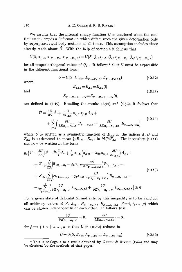
t 30 A . E . GREEN & R. S. RIVLIN:

We assume that the internal energy function U is unaltered when the con- t inuum undergoes a deformation which differs from the given deformation only by superposed rigid body motions at all times. This assumption includes those

already made about U. With the help of section 4 it follows that

U(S, Xi, A, XiB,...By , XiB,...By,A ) = U(S, Qi/Xi,A, QiiXiB,...B~, QiiXiB,...Bv,a)

for all proper orthogonal values of Qii. I t follows* tha t U must be expressible in the different functional form

where

and

are defined in (4.19).

0 ou g ou x - = ~ "3 t- ~ i,A X/,BZtij +

U= U(S, E:AB, EB,..B~,:A , EB,...B~,:A~: ) (t0.t2)

E:aB=EAB=EaB(t), 00.t3)

EB,...8,:A,...Ac,=EB,...B,:A,...A,, (t) ,

Recalling the results (4.3t) and (4.32), it follows that

r= 1 0 E B .... B~,:A BB'"'B~:A "j OE, B .... B~:AK

(10.t4)

where U is written as a symmetric function of EAB in the indices A, B and EAB is understood to mean �89 +EBa ) in OU/OEAe. The inequality ( t0 . t t ) can now be written in the form

+ XA,i = ~B,...B#--OoXi,B OEe .... Bo:B . . . . (1o.15)

a~_'l( 0u 'B -~- XA, i Y~KiBt...Ba--eoXi,B OEBx-~..-B#:BK- ) Bx...B#:AK--

- -& OEm~ff.B#:A Be'"'~#:A-+ OEB,..B~:AX Be'"'B~:A~: >0 . #~v+l

For a given state of deformation and entropy this inequality is to be valid for

all arbi t rary values of S, Ami, BB1...B~:A, BB1...B~:AK ( f l = t , 2 . . . . . /~) which can be chosen independently of each other. I t follows that

OU OU - - 0 , - - 0 ,

OEBI... BB:A OEB~ ... BB:AK

for f l = v + t , v + 2 . . . . . /, so that U in (10.t2) reduces to

U= U(S, Fan, EB,...Ba:A, E~,...B p :ate) (10.16)

* This is analogous to a result obtained by GREEN & RIVLm (1964) and may be obtained by the methods of that paper.

Multipolar Continuum Mechanics t3t

with fl = t, 2 . . . . . v. In addition, T - - ~U a s ' (t0.t7)

, ~u (to.t8) ~Kra=2OoXm'A OEAK '

- - aU (t0.t9) ~7~iBt...B# ~ 00 Xi ,B ~EB1. . .B~:B '

~U (t0.20) Y~KiB~...Bp ~ O o X i , B ~EBx. . .B~:BK ,

the last two results holding for /5 = 1, 2 . . . . . v. Also

--q~T~>__0 (1o.2t) and with the help of (10.17)--(10.20) equat ion (9.t9) reduces to

00 r - - qK, K -- 00 T S----- 0. (10.22)

Because of (10.9)~ and (10.t8) equations (9.16) and (9.t7) are satisfied identically.

If we introduce the Helmhol tz free energy function

A = U - - T S (10.23) and express A in the form

A = A ( T , E A B , EBI . . .Ba:A , EB~...Ba:.4K) , (t0.24) then

S - - 0.4 aT ' (t0.25)

, aA (t0.26) 7rKm = 200 X~'A 0EaK '

_ ~A (10.27) 7giB~...B# ~ OOXi,B ~EB~...Ba: B '

~A (to.28) 7gKIB~...B# ~ 00 Xi ,B 8EBx... BB:BK "

Equat ions (9.14) and (10.27), together with (9.5), form a basic set of equations of mot ion for the stresses ~rri and mult ipolar stresses ~rKiB~...B ~, the const i tut ive equations for these stresses being given b y (10.26), (t0.28) where, f rom (9.t3)

v

~ra ~ = n~ m + )Ca,~ Y (~B,...Ba X~B,...Ba + ~m~,...B~ x ~ , . . . a a , r ) . (t0.29)

11. E las t ic i ty : a l te rna t ive f o r m

Before considering const i tut ive equations of a more general type, based on the work of section 8, we obtain results for elasticity in the nota t ion of section 8. We suppose tha t the con t inuum is in a reference state X B at t ime t o and we assume tha t the internal energy U at some time T (to<=T<=t) has the fo rm*

U(T)=UES, x~,a(~),x~j,., j~(~),x~j,., j~,k(~),xi, a,x~j,..j~(to),X~j,...j~,k(to)] (11.t) * Although U(T) is expressed in terms of the variables in (11.1) for convenience

in this section it must essentially be such that it is a function of kinematic variables at times T and t o.

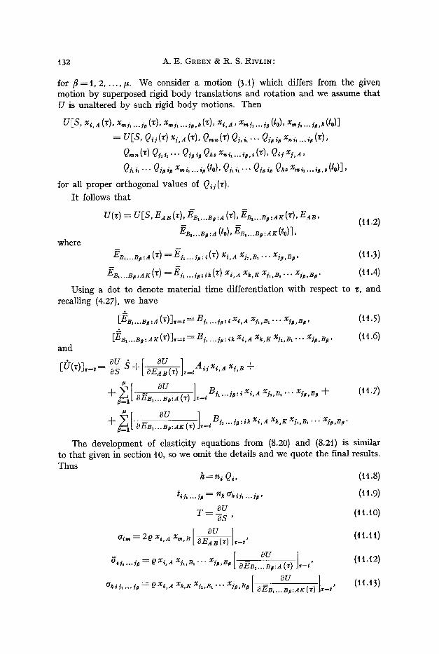
132 A.E. GREEN & R. S. RIVLIN:

for f l = t , 2 . . . . . /~. We consider a motion (3.t) which differs from the given motion by superposed rigid body translations and rotation and we assume that U is unaltered by such rigid body motions. Then

u [ s , xl,4 (r), x,~j . . . . ;p (3), Xmj .. . . /p,k(3), X~,4, Xm/ .... /~(tO), X,~i . . . . ip,k(to)]

= u [ s , Qi j(3) xj, 4 (3), Qm, (r) Qj, i , . . . Qj, ~, x ,~ .... ~ (3),

Qm.(*) Qj,,,. '- Q/,~, Q~, x.i .... i~,.(3), Q . x,-4, Qj, i , - . - Qi, i~ xmi ... . 4, (to), Q/,~, . . . Qj,~, <2~, x . ~ .. . . i , , , ( to)] ,

for all proper orthogonal values of Qii(3).

It follows that

u(T} = u [ s , ~ 4 B (3}, ffB,. . .~,:4 (3}, ~ , . . . ~ , . . 4 ~ (3), E 4 ~ , ( t t .2)

E~....B, :4 (to}, ~, . . .~ , :4K (t0}], where

/T~, . . .~ :4 (3) = ~. .... j,.. ~(3) x i ,4 x / , ~ . . . x / , ,B , , ( t t .3)

/~B,...~#:AK(3) =/Ti .... i#:~,(~) Xi, 4 Xk, n Xi,,B ' ... Xi#,B #. (tt.4)

Using a dot to denote material time differentiation with respect to 3, and recalling (4.27), we have

[EB,...B#:A (3)],=,= B i . . . . i#:~ x~,4 x i , , B , " " Xi#,B#' (11.5)

[EB, . . .B# :a lC(3) ] ,= t= B i .... i#:~,xi,4 x , ,g xi,,B , ... x/a,B #, (11.6) and

~U ~ + [ ~U ] , = A i i x , , 4 Xi,B + [O(,)],=t = ~ ~Ea B (,)

+ 0EB .... B#:4(~) ]~=~ Bi .... i#:iXi'a Xi~'~'"" Xia'B# + (tt.7)

The development of elasticity equations from (8.20) and (8.21) is similar to that given in section 10, so we omit the details and we quote the final results. Thus

h = n~ (?~, (1 t .8)

tiJ .... i # = n * a * i i . . . . /#, (1t .9)

T - - OU (ltA0) ~S '

[ ~ v ] , 0 1 . 1 t ) aim = 2e x, ,4 Xm,B [ OE4 B (*) Jr=t

~,i .... i #=~x , ,4 xj,,B...x~.,,~,[- oU 1,=, (11.t2) ~E~ .... B#:a (*)

[ 0u 1 ( ~ . ~ } . . . . . . . .

Multipolar Continuum Mechanics t 33

where U is given by (11.2) and fl in (tl.2), (11.12), ( t t . t3) takes the values 1,2 . . . . . v. Also

- -Q, T i>=0 (11.t4) and

9 r - - Q i , ~ - - q T S = O . (11.t5)

The expression for U is symmetrized with respect to the indices A, B in EaB(z ) and EAB(* ) is understood to mean �89 ) + E B A (,)] before (11.1t) is used, and then the symmetry condition (8.t9) is satisfied. In view of (tt.9) the condition (8.t8) is satisfied identically.

12. Constitutive equations* For convenience we collect here all the fundamental equations of section 8,

namely (8.6), (8A6), (8.t7), (8.19), and (8.21), together with (8.7), (8.14), (8.18), and (8.20), and the entropy production inequality (8.3). Thus

~,.~.j + q F~ : q v! ~1, (12.t)

a~J . . . . i~ = q ~ J . . . . i~ + a ~ i J . . . . i p , * , (12.2) v v

a i '* = a m i = a i r ~ - - a ~ i . . . . iB X'nJ . . . . i~ - - akii . . . . i~ xmJ . . . . j ~ , k , (t2.3)

B = I

+ ~ a k i i . . . . ia Bj . . . . i a : i k : O , B=I

and

, , - ~ n4a , i$ ,

7~=h-ni Qi, ~*~, . . . #a = t i i, . . . ia - - n ~ a k i i , . . . i a ,

E (i,j .... i , x . j .... j , - t L j .... i x,j .... j , ) = 0 , B = I

(12.4)

(12.5)

(12.6)

(12.7)

(t2.8)

(12.9) TdV + f TdA >=0. fe~dV_fe r h V V A

1 transforms as a tensor of order In equation (t2.8) B i . . . . ia :~- -~Am~x,~ i . . . . ia

f l + l under changes of rectangular cartesian axes. We assume that iii .... ia also transforms as a tensor of order fl + t and that h is a scalar, under change of axes, so that the left hand side of equation (t2.8) is then a scalar. Since, for a given surface, tii .... ia is a tensor and h a scalar, it follows from (t2.6) tha t Q~ transforms as a vector and ak i i . . . . i~ as a tensor under change of rectangular axes, where the appropriate quantities in each system of axes refer to the

* See also section 16. Arch. Rational Mech. Anal., Vol. 17 10

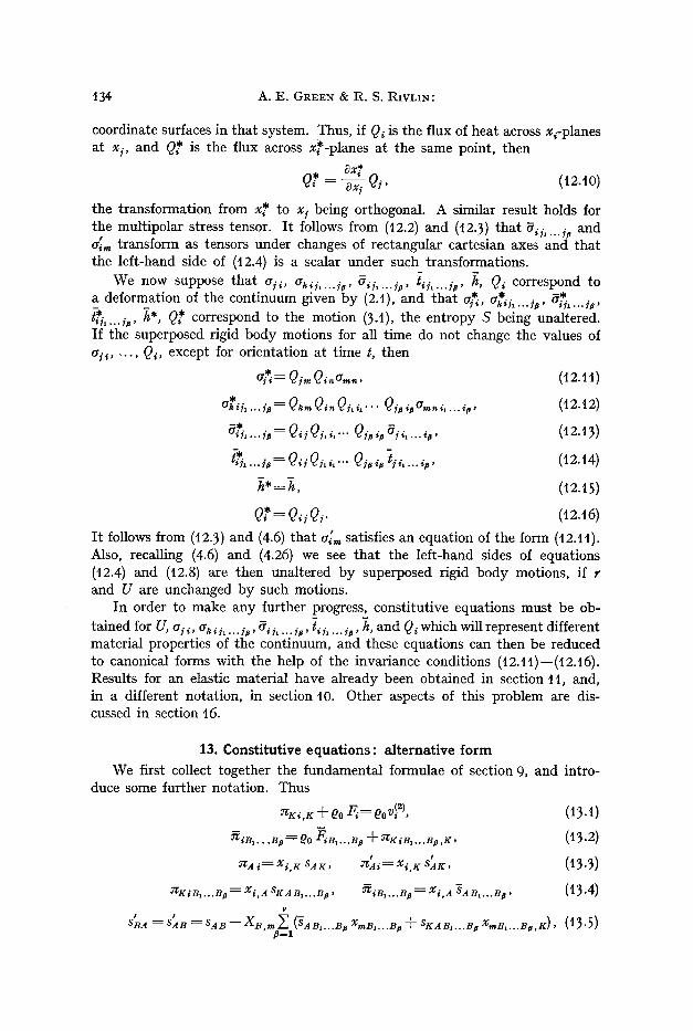
t 34 A.E. GREEN & R. S. RIVLIN:

coordinate surfaces in that system. Thus, if Qi is the flux of heat across xi-planes at x i, and Q* is the flux across x*-planes at the same point, then

Ox* Q* = ~ Q j , (t2.t0)

the transformation from x* to x~. being orthogonal. A similar result holds for the multipolar stress tensor. I t follows from (12.2) and (t2.3) that aii .... ia and a ~ transform as tensors under changes of rectangular cartesian axes and that the left-hand side of (12.4) is a scalar under such transformations.

We now suppose that a]~, ak i i . . . . ia, a i i . . . . ia, t~i . . . . i~, h, Qi correspond to e.*. a deformation of the continuum given by (2A), and that a* , a*ii . . . . ]~, ,~ . . . . ip,

~* .... jp, h*, Q* correspond to the motion (3A), the entropy S being unaltered. If the superposed rigid body motions for all time do not change the values of ai , . . . . . Qi, except for orientation at time t, then

a*ii . . . . ia = Qk,,,Qi,~Qi, i~... Qi, ipa.....i .... ia. (12A2)

e* .... j~ = 9 , Qj, ~.-. 9j~ ~, ej~ .... ~,, (t 2.13)

/.'* -- (t2A4) , .... ~.p- Q,.Qj,~,... (?,.,~ t;~ .... r

~*=7,, 02.15)

Q * = Q i i Q i . (t2A6)

I t follows from (12.3) and (4.6) that a/'m satisfies an equation of the form (i2. t l ) . Also, recalling (4.6) and (4.26) we see that the left-hand sides of equations (t2.4) and (12.8) are then unaltered by superposed rigid body motions, if r and U are unchanged by such motions.

In order to make any further progress, constitutive equations must be obtained for U, a si , a~1 .. . . ~ , a i i . . . . ~ , ti1 . . . . ~ , h, and Qi which will represent different material properties of the continuum, and these equations can then be reduced to canonical forms with the help of the invariance conditions (t2A1)--(12.16). Results for an elastic material have already been obtained in section t l , and, in a different notation, in section 10. Other aspects of this problem are discussed in section 16.

13. Constitutive equat ions: al ternative form

We first collect together the fundamental formulae of section 9, and introduce some further notation. Thus

~:~,~ + eo F~= ~oV! ~), ( t3.t)

~ iB . . . . Bp = ~0 ~B, . . .B ,6 "I- :7~K iB1...B,8,K ' (13.2)

~a ~= xi,~, sa ~, ~ = x~.~ s ~ , (t 3.3)

~7~KiB,...B a : X'i,A SKABI . . .BB, ~iB1...BI~ : Xi , A "SAB1...BI~, (t3.4) v

s'~a = s'aB = s , B - z ~ , , ~ y (~ , ,~ , . . .~ , x,,,~, .,~,, + s~:,,~,. .~ , x,,,,~...B~,~:) , (13.5)

Also, if

then

Multipolar Continuum Mechanics

qO ~ 1 ' - - 2 V ~ S K A Xra,A x~,KA,,i + Qor--qK,r v

+ ~ (saB,...Be BB,...Be :a + S~aB,...Be BB,...Be.A~) = 0. B=I

t35

(t3.6)

p~=x,,ara, PiB,...Be=Xl,araB,...Bp, piB,...Be=Xi,A~aB,...B,, (13.7)

rA=NK SKa,

ho= ho -- Nr qg , (13.8)

~A B, . . . B e = J'A B , . . .B e - - N K SKA B1...B e '

~ , ~ AB , . . .Be (Xi , A XmBa.. .Be - - Xm, A XiB, . . .Ba ) .~---0, (t3.9) ~=1

~. ~aB,...Be (BB,...Be:A --~Amixi,aX,nB,. . .Be)--ho=O, (t3A0) and a=x

foogdro-fQo- dro +f dAo>=o (13.,t) V, vo Ao

1 In (t3A0), BB,...Be:A--~A,,iX~,aX,~BI...Be transforms as a tensor of order fl + t under changes of rectangular cartesian axes and is also unaltered by superposed rigid-body motions at all times. We assume that raB,...Be is unaltered by these rigid body motions and that it transforms as a tensor of order fl + t. We also assume that ho transforms as a scalar and is unaltered by superposed rigid body motions. I t follows that the left hand side of equation 03.t0) is a scalar which is unaltered when rigid body motions are superposed on the given motion. Since, for a given surface, rAB,...Be is a tensor and h 0 a scalar, it follows from (13.8) and (13.4) that SKaB,...Be and ~ K i B , . . . B e transform as tensors under changes of rectangular axes, and that qr transforms as a vector, with respect to all indices including K. Also, from (t3.2), (t3.3) and (13.5) we see that ~iB,...Be, ~a~, SAB,...Bp and s~K transform as tensors under changes of rectangular axes and that the left hand side of (13.6) is a scalar. Moreover, BB,...Be'. A, BB,...Be: A K and X,~,A Xi,K A,~ i are unchanged when superposed rigid motions at all times are added to the given motion. We therefore assume that SKAB,...Be, S--aB,...Be, S'Ba, qg, U, and r are unaltered by such rigid body motions. I t follows that sBa and the left hand side of equation (t3.6) are also unaltered.

Constitutive equations must now be postulated for s'~a, SAB,...Bp, SKABI...Be, qK, U, raB,...Be and h0 which will represent different material properties of the continuum and these equations can then be reduced to canonical form, with the help of the condition that they are all unaltered when rigid body motions are superposed on the given motion.

Results for elasticity have already been obtained in section t0, but we add here some other results derived from (10.8)--(10.20), and (t3.3) and (t3.4), namely

, , OU SKa = SAK = 2~0 , (t3.t2)

~ E A K ~u

S A B , . . . B a = eO OEB, . . .Ba : A , (13.13)

~u (t3.t4) S K A B , . . . B a = ~0 OEB . . . . Ba:AK

! O*

t 36 A . E . GREEN & R. S. RIVLIN:

14. Elast ici ty: relation to previous theory

In a previous paper (GREEN & RIVLIN, t964) which was concerned with the theory of simple multipolar forces and stresses of the first kind, associated with monopolar displacements and velocities, explicit formulae were obtained for elasticity. We now show that these elastic equations can be obtained as a special case of the present theory, and for this purpose we use the form of the theory given in section 10.

The tensors EB,...Ba: B and EB,...Ba_I:BB ~ may be expressed in the form

EB,...B~ :B = E(BI...B~):B + EB,...B~ :B, (14.1)

EB,...B#--, :BBII = E(B,...B~--I):B(Bp) ~- E* ...BI3_a :BB#,

for fl----2, 3 . . . . . v + t , where E(B,...B#): B is the part of EB,...Ba: 8 which is completely summetric with respect to B x . . . . . B~ and E(B1...BII_,):B(B#) is the part of EBx...Ba_x:BB # which is completely symmetric with respect to the same indices. The tensors E* . . . are then defined by (t4.1). With a similar notation we also have

~iB , . . .B a = ~i(B, . . .Ba) ~- ~ * i B t " ' B a ' (14.2) :r~B~ iBx...B~--x = ~(B~) i(B~...Bp_~) ~- ~ B a iBx...BB--t,

for f l=2 , 3 . . . . . v + l . Equations (t0.19) and (t0.20) may now be written in the alternative forms

a u (14.3) ~i(Bx...B#) ~- ~0 Xi ,B aE(B . . . . B0): B '

a u (14.4) Sg(BB)i(Bx...B#_~) ~--- ~0 Xi ,B OE(B~... Be--x): B (B#) '

~*B,...B~ = qo Xi,s aU (14.S) OE~ . . . . BB : B '

, 8 U :TgBBiBt...BB__x = qOXi,B , , (t4.6)

OEBx... B~--I : BB~ for f l = 2 . . . . . v + t , and

OU 7giBx = ~0 Xi ,B OEBa:B ' (t4.7)

, 8U ~Ki = 2~o Xi,A ~ E A K �9

In (t4.3) and (t4.5), 8U/OE(B,...Ba): B denotes the par t of OU/SEB,...Ba: B which is completely symmetric with respect to B 1 ... B a and 8U/OE*.. .Ba:B denotes the remaining part. Similar notations are used in (t4.4) and (t4.6).

Next we take special values

XiB,...B~ = Xi,B,...B~ (fl = t . . . . . v) (t4.8)

for the multipolar displacements. I t follows from (4.t9) and (t4.1) tha t

E(Bx '"Ba):B = E B B ' ' " B ~ ' (14.9) E(B,.. . B a _,) : B (B~) = EBB, . . . B a ,

for f l = 2 . . . . . v in 04-9h, f l = 2 . . . . . v + t in (t4.9)z, and

EB, :B = EBB, =EB, B, (14.t0)


is defined in (3.6) and is completely symmetric with respect

(14.1t)

oU 8EBBx ... Bv+t

8U aEBBt... BB

for fl=- 2 . . . . . v and 3u

~EBB~

___ ~u (14.13) 8E(B~ ... B~): B (B~+I) '

_ ~ U + 8U (t4.t4) OE(BI ... B~--I): B {Ba) OE(Bx ... Ba): B

0u 0u (14.15) - - 8EBBI -~ 8EB~:B "

From (14.4) and (14.t3) we have

0U (14.t6) Jg(B,,+t) i(B~...B,,) = ~0 Xi, B OEBBI... B,,+I "

Again, from (9.14), (t4.3), (t4.4), and (14.14), we obtain the formula

- 0U (14.17) ~(B$)i(BI...Bp_,) ~- :r~Ki(B,...B~),K -~ ~0 Fi(Bt...B~) = ~0 Xi,B OEBB ... . B~

f o r / 5 = 2 , ..., v. Next, from (9.t3), (9.14), and the formulae of this section, we see that

~gAi 2V ~rgKiA,K2V OO~A - - v + l

OU oU (v>=1). (14.t8) = 2q0Xi,B ~--~-AB + q0 s OEAB~,...Ba Xi'B'"'Ba

fl=2

In deriving (14.t6)--(t4. t8) we have assumed tha t U takes a definite value when conditions (14.9), (14.t0) and (14.tt) apply, and that the derivatives

of U in (14.16)--(t4.18) can be evaluated. Formulae (14.5) and (14.6), however, contain derivatives of U with respect to the tensors EB,...Ba :B and EB,...Ba_~:BB ~ at the zero values of these tensors. If U depends on elastic coefficients which

* E* tend to zero, in such a way tend to infinity w h e n EBt...B#: B and B,...B#--I:BBB that U tends to the value (t4A2) but the right hand sides of (t4.5) and (t4.6) tend to arbi trary functions, then the values of * and ~* ~B~ iBm...Bp--t i Bx...BB are undetermined. This situation is analogous to that which arises when equations for incompressible elasticity are derived from those for compressible elasticity by a limiting process. Equations (t4.16)--(14.18) agree with those obtained previously (t964) except for a change in notat ion.*

* The inertia terms were not included explicitly in the previous paper.

where EBB,...B~ to B 1 . . . . . B~. Also

* = 0 , * EB1...B a :B E Bt...Ba_ z :B Ba = O.

The function U in (10.t6) reduces to

U ( S , EAB , EB,...B a:A, EBt...B~:A K) = U ( S , EAB, EAA .... A,,) (say) (t4.t2)

where/5 = t . . . . , v; g = 2 . . . . , v + 1, and 0 is expressed as a symmetric function of EaB and of E A A .. . . A,, as far as the indices A1, . . . , A are concerned. From (14.9) and (14.12) we see that

t38 A.E. GREEN & R. S. RIVLIN:

15. Infinitesimal elasticity

Elasticity theory appropriate to a continuum in which the displacements and multipolar displacements are infinitesimal can be obtained at once from section t0. For simplicity we restrict our attention here to the theory in which only displacements and dipolar displacements, and their corresponding stresses, are present. Then, using the Helmholtz function A,

A = A ( T , EaB, EB:a, EB:AK), (15.t)

, 0A (t 5.2) ~Km = 200Xm,A OEAK '

OA ~iB ~ OoXi,A ~EB:A ' (t5.3)

OA 9IKiB = O0 Xi,A OEB:AK ' (15.4)

~x~,~=z4~x~,~ , (15.5)

x~ ~ = ~A ~ - x ~ , ~ ( ~ x ~ + x ~ x~B,~) , (15.6)

~ , = eo if/, + ~g iB,X, (t 5.7)

:~i,,~ + eo Fi = eo V! ~), (t 5.8)

S ---- ~A OT' --qKT, K>=O' (15.9)

eo r -- qtc,g -- eo T S = 0, (15 A0) and

#i=Ng uKi, ho=N2c qK, (t5At)

In ( t5A) , EA B = XI ,A Xi,B,

EB:A=Xi,AXiB, (t5.t2)

EB:AK ~- Xi,A XiB,K"

Let Xia denote the value of xia in the reference state X a and let

EAB = EaB -- (~AB,

EB:A-'~EB,A --XAB, (t 5.t3)

E B : A K = E B : A K - - X A B , K �9

We shall consider that A is a polynomial in EaB, ~Ts.'a and ~Ts..A/~ and if these latter quantities are small enough we may approximate A by*

Oo A = C + x a B L B +flBa L : a -~-~)BAK~:AK-~-

+ (15.14)

�9 We assume here that the temperature T is constant. Alternatively, if we replace A by the internal energy U then the entropy S is constant.

Mul t ipo la r Cont inuum Mechanics t 39

where C and the coefficients aAB . . . . , ~ABCDEF are constants if the body is initially homogeneous. We may omit the constant C without loss of generality. If, when the body is in its reference state, n ~ , ~ B and nKiB vanish and the body is in equilibrium under the action of no body or surface forces, and no multipolar body or surface forces, then 0~aB, flAB, 7BA~ in (t 5.t4) are zero and A reduces to

. . . . . (15.15) "~- ~ABcDEA : B E c : D - ~ A B c D K E A :B EG:DK2V~ABGDEFEA :BC ED:EF,

where without loss of generality

ZA.C~ = ;t.a c ~ = aA..C = ~C. . a ,

IAABCD.-'-=IABACD, VABCDK'--~VBACDK, (15.16)

We now write

x~=X~ + e ui, (15.17) Xia ~ X~a + e Uia,

in the expressions (15.13), and neglect terms of higher degree than the first in e. We then obtain

F--~ A B = $ (C~ A,B "+ UB,A) -~- e A B,

E~ :a = ~ (ua B + u~.~ X , . ) = / B a , (15.t8)

If we introduce (15A5) into (i5.2)--(15.4) and use (15.t3), (15.t8) and retain only terms of order e, we have*

~r'Kr~=Z(22KmCVeCZ)+IAKr~CD/CD+VKraCDL/CDL), (t5.19)

~iB =iAco~ieco + 2~B~Cn/CD + ~ISICDK/CDtC, (15.20)

~KiB =VCDBiKeCD + rtCDBiK/CD + 2~BIKCDF/CnF. (15.2t)

Also, from (15.5) and (t5.6), we have, to order s,

t r ~im = 7rml , (15.22)

~a ~----n]~ + ~r-a B X~B + ~rga BX,~,u. (t 5.23)

If the continuum in its undeformed state is isotropic with a center of symmetry (holohedral) then the coefficients in (t 5.15) take the special forms

42ABED -~- 2 0ABOc o 2VIA ((~A C(~B O 2V (~A D (~BC), (15.24)

IAaBCO = aX~a Bt~CD +IA1 (~a CtSBD + ~a 3fgBC), (15.25)

2~ABCD=~I (~AB(~CD'~-~OA COBD-~ ~aOA DOBC, (t5.26) * W e can also p u t , = t now wi thou t loss of genera l i ty . A m u s t be wr i t t en as

a symmetric function of EAB before equation (15.2) is used.

t40 A.E . GREEN & R. S. RIVLIN:

+ G(~A c ~s9 ~EF + ~D~ ~A E ~SC) +

+ ~ , ( ~ ~s~C9 + ~B9 ~Ce ~A ~) + (15.27)

+ r ~cF~e + ~ ~AC~Be~DF +

-~ r dA F (~BE OCD'

VA~CDK=rl~SCDK-=O, (15.28)

where the coefficients 2, # . . . . . ~1 are constants when T is constant. The expressions (t 5.19)--(t 5.21) then become

~Km~--2OKmecc'q- 2/ZeKm-~ 22IOKm/CC @ 2/Zl(/Km-~ /mK), (t5.29)

~ = 2~ dis e c c + 2/Zl ein + ~1 O~n/c c + ~e /~ i + ~ ~is, (15.30)

~ = ~ (~s//~ov + O~/~/~s) + r + ~sKlz~v3 +

+ G('~Hwo + '~sK/.~v) + r +h~:s) + (t5.3~)

+ ~8/BiK "q- r + r + r We consider one simple application of these results. Suppose Xis is con-

stant and that we have a homogeneous deformation

ui=-biaXa, bA4-=biA, (t5.32)

with constant values of the dipolar displacement uas. We suppose that the body is in equilibrium under the action of zero body and dipolar body forces. Then

/SAK=O, 7"f'KiB=O, eA~=2ban, (t5.33)

and, from (15.7), we must then have

~ s = O. (15.34)

Equation (t 5.34) can then be satisfied if

21(~+~) --2~1/zl OiSeDD (15.35) (~ + ~.)/~s = ( ~ + ~ ) / s ~ : - 2~1 e~s - 3 ~1+ ~ + ~ provided

3 ~ : ~ + ~ + ~ + 0 , ~-1- ~3 4= 0. (t5.36)

From (t5.32), (t5.35), and (t5.29) we see that n}~ are constants and, from (t5-23)

~a m = ~ra,~ (t 5.37)

so that the equations of equilibrium (t5.8) are satisfied. Equation (15.35) gives the dipolar displacements in terms of the homogene-

ous deformation coefficients bia. Such a deformation can be maintained by the application of surface forces alone and no dipolar surface forces at the boundary of the body.

Multipolar Continuum Mechanics 14t

Since eiy,...y a follows that

16. Equations of motion and variational equations

TRUESDELL & TOUPIN (t960, sections t66, 205, 232) introduced the idea of a generalized velocity, which in our terminology is called a multipolar velocity and corresponds to (4.11), but they did not include the restriction (4.t4) which describes the behavior of such a velocity when rigid-body motions are superposed on the continuum. They defined generalized body and surface forces and stresses, called here body and surface 2a-pole forces of the (f l+ 1) th kind and surface 2&pole stresses of the (fl + t) th kind, and they postulated equations of motion and an equivalent variational equation. In this section we examine the relation of the ideas of TRUESDELL & TOUPIN to those presented here and for this purpose we use the basic equations of sections 8, 12.

The condition (4.6) on multipolar displacements, or the equivalent condition (4.14) on multipolar velocities, under superposed rigid body motions implies, in particular, that multipolar displacements and velocities are unaltered by superposed rigid body translations at any speed, and at any time. This condition, together with the other assumptions made in section 8, enabled us to obtain the classical equations of motion (8.5) from the energy equation (8.t). Without this condition the classical equations (8.5) would not have the same form.

Because multipolar displacements and velocities are unaltered when the continuum receives superposed rigid body translations at any speeds, it is possible for the quantities U, a~**, akij .... j~, aij .... i~, and Qi to depend explicitly on these displacements and velocities but not, of course, on the ordinary monopolar displacement and velocity which are altered by rigid body translations at various speeds.

We now consider the special situation in which U does not depend explicitly on multipolar displacements or velocities and a ~ , aki j .... ]~, aiy .... y~, Qi (and r) do not depend explicitly on multipolar velocities. We consider a second motion of the continuum which is such that its position and the multipolar displacements at time t are unaltered, but it now has multipolar velocities v i i . . . . Ja + v'i] . . . . yp

(fl = t . . . . . v), where v~ ] .... ]a are constants (in space and time). The corresponding energy equation will differ from (12.4) only by arbitrary constant values v~] .... Ya added to B y .... ]a:i so that, by subtraction,

v t

aiy~.. . Ya v i i . . . . Ya ~ O. 8=1

is independent of v~y .... ia which can be chosen arbitrarily, it

o r

a iil.., ia = 0

ak~] . . . . Ja,~ + ~ i . . . . /a = 0 ' (t6.t)

If we recall (8.2), we see that (t6.t) are the equations of motion postulated by TRUESDELL & TOtlPIN (t964, section 205). It should be emphasized that these equations are not always satisfied, and, in particular, are not necessarily satisfied for an elastic medium, as is seen by ( t t . t2) when U depends on multipolar displacements.

t 4 2 A . E . GREEN & R . S. RIVLIN:

Again, if h and //i .... ip do not depend explicitly on multipolar velocities, we can show, from equation (t2.8), that

tii, . . . /p=0 o r

tii .... ia = n~ akii .... ia" (16.2)

Equations (t6.2) were postulated by TROESDELL & TOUPIN (1964, section 205). From (12.8) it then follows that h = 0 or

h- - -n iQi . (16.3)

We have established sufficient conditions under which the equations of motion (t6A) and the surface conditions (t6.2), postulated by TROESDELL & TOUPIN are valid. Since these equations are completely equivalent to the variational equations studied by TRUESDELL & TOUPIN (1964, section 232), we have also established sufficient conditions under which the variational equations hold. In general, however, the variational equations are incomplete unless they include variations of the internal energy and the heat conduction vector.

Throughout this section we have assumed that the multipolar displacements and velocities of all orders are independent and we have not considered de- generate or special cases. For example, if multipolar velocities have the special gradient form

v~i .... i~=v~,i .... i~ (16.4)

then equation (t6.2) would still follow if we assume that /~ and t"ii .... ip do not depend explicitly on velocity gradients of all orders, as shown previously by GREEN & RIVLIN (t964). Even if we assume that U does not depend explicitly on displacement or velocity gradients and that a~,,,, aki i .... ip, e l i .... ip and Q~ do not depend explicitly on velocity gradients we do not obtain equations (t6A).

17. Appendix

We suppose that N particles with masses m IP} (P = t, 2 . . . . . N) are situated at the points X ! P} at time t 0. At a subsequent time v (to_~ T<~t) we assume that the masses are at points x! P} (3) (P = 1 . . . . . N) and we use the notation

x (P) - - x (.v) (t) (P) (v) X~ =x~ (to) (t7.0 $ - - $ ,

The center of mass G of the N particles at time ~ is denoted by xi(z ) where N N

M x i (3) -- Y. m IP) x! P) (z), M = Y, m IP) (t 7.2) P=I P=I

and we write

If

then

x ~ = x~ (t), x ~ = x~ (to). (t 7.3)

y!PI (3) = . ! P ) ( 3 ) - .,(~),

Y ( P ) - - ~ f l v ) t t ~ - - X ( v ) X i - - ] i k O] -- ) - - i ,

(t7.4)

N Z m (PI y!~l (~) = o ,

P = I

N

Y. m I~) y!~) = 0, P = I

N

(17.5)

Multipolax Continuum Mechanics t43

The motion of each particle and the motion of G is given by

�9 ! P) (~) = ~!~)(% x ~ ) ) ,

x~(~) = x~ (~, X , ) , or by

since

�9 !~> (,) = ~!~)( , , t, ,~v)),

xi(*) = xi(*, t, x , ) ,

(t7.6)

(17.7)

v! ~) (~) = ~!P)(r) = vi(r) + p!e)(T), (t 7.9)

where a dot denotes derivative with respect to r holding X~ P) fixed in (t7.5) or t and x~ P) fixed in (17.7), and v~(z) is the velocity of G. We use the notation

v! ~) = v! p) (t), v , = v,(t) . (t 7.t0)

It follows from (t7.2) that N

/ v i ( r ) = Y. m(V)v! P) (7:), ( t7. t t ) P = I

and, from (t7.5) N N

Y. mW)~!P)(r) = 0 , Y. mW)~v)=0. (t7.12) P = l P = I

Suppose each mass is acted on by a force Fi(v)(r) per unit mass, where

F~c~) (~) = ~,(~) [% ~) (~) ] .

In view of (t 7.4), (t 7.6) and 07.7) this can be expressed in the alternative forms

F/(v) (r) -- F~ w) (r, X, + y W)) (t 7. t 3) o r

Fi (P) (r) = F~ (P) (z, t, x, + y~P)). (17.14)

The rate of work of these forces is

N

W = Y. m w) F/(P) (r) v~ P) (r). (t 7.t 5) P = I

Adopting the form (17A3), we define a continuous function of z and X,+Y, , F*(z, X,+Y,) say, with continuous derivatives up to order / , + t, such that

F~* (,) = ~*( , , X,), F~(~) (,) = ~ * (,, X, +Y,(v))

for each value of P. Then,

~ x l E * .. Fi(P)(v)=Fi*(r,X,)+ ~.f ,,B,...Ba(r,X,)Y(f). Y(~)+R,, (t7.t6)

The velocity of the mass m (P) at time z is defined as

xlv)- xW)/t X~V)), 07.8)

x~= xi (t, X,) .

t 4 4 A . E . G R E E N & R . S. R I V L I N :

where R i is a remainder term and ~F~* (~)

~%,...,~ (w, x , ) - ~ x , ~ . . . ~ x ~ �9

From (17.15) and 07-9) we have N

W = i F i (w) v i (w) + Y~ m (v) Fi (P) (w) ~!v)(w), P = I

where

(17.t7)

07.~s)

N MF/(w) = ~, m IPI Fi cvl (w). (17.19)

P = I

If we substitute (17.16) into (17.18) and use 07.t2) we see that

p

W =-- MF~(w) vi(w ) + M~, Fi*B,...n~ @, X,) ViB,...B~ (W), (t7.20) 8=1

if the remainder term can be neglected, where

N MV,B,...B~(W)= ;! ~, m(P)~!P)(-C) Y(BP) ...YCB P). (17.2t)

"P=I If we define xiB,...~ (w) by

N M XiB ..... 8, (7:) = ~_ ~, m CP) y!V)(7:) Y~(BP)... Y(B P), (17.22)

r " P = I

then vie,...Bp (W) = XiB,...B~ @)" (t 7-23)

We observe that XiB,...B~(W ) satisfies an equation of the form (4.2), when all the particles receive an additional rigid body motion, for all times w. In particular it is unaltered when all the particles receive the same additional translation or translational velocity. Regarded as a function of w and Xr the expression XiB,...B~ (W) in (17.22) is a special case of the multipolar displacement defined in (4.1) and (4.2). The form (t7.22) is completely symmetric in B 1 . . . . . B B .

We now define a continuous function of w and X , + Y,, x~(w, X, + Y,) say, with continuous derivatives up to order/z + t, such that

x* (w) = x* (w, X,) and X! P) (T) = X~ (W, X r -~ Yr (P))

for all values of P. Then,

/*

:Y!P)(w)= y,_x~Fv*a,...A~,(w,X,)YJP)...Y(aV,'+ Ri, (17.24)

v,(z) = ~ ' ( w ) .

With the help of (17.24) the rate of work (17.18) becomes

W---- MFi(w ) vi(w ) + ~, Fi:a,...a, (w) V~, A .... A.(Z, X , ) (17.25)

if we neglect the remainder term, where

N

Fi.A ' A.(W ) = 1 N-~ m(p)E(p)(.r~y(f) yj~). ( 1 7 . 2 6 ) .... ~! f'~----I * ~i "'"


The tensors Fi: a .... a,(z) are 2~-pole body force tensors of the first kind. Equa- tions (t7.20) and (17.25) show that the rate of work of 2~-pole body forces (~ = 1 . . . . . #) of the first kind is equal to the rate of work of monopolar force gradients in multipolar velocity fields.

Equations (17.2t) for f l = t , 2 . . . . . #, together with the first set of equations in (t 7.t2), may, for a given value of i, be considered as ] (# + 1) (# + 2) (# + 3) equations for N velocities ~!PI (T) (P = 1, 2 . . . . . N). If

(# + t) (# + 2) (/~ + 3)>_--N (t7.27)

we can, in general, express ~!vl (~) as a linear combination of multipolar velocities ViB,...Ba(7: ) (/5=~, 2 . . . . . #). When ~ ( # + t ) ( / ~ + 2 ) ( # + 3 ) > N there will be rela- tions between these multipolar velocities. Thus

/J

N!P) (T) = E YA(P).. A , V/A . . . . A , ( ~ ) , ( t 7 . 2 8 )

where YA CP). .A, is completely symmetric in A 1 . . . . . A~ and depends on Y(B P) and m (P). Some of these coefficients may be taken to be zero when ~ (/~ + t) (/~ + 2) (# + 3) > N.

The kinetic energy T of the N m a s s e s m (P) is given by

N 2 T = ~. m IPI v! P) (~) v! P) (7:)

P=l (17.29) N

= M ~, (,) ~ (,) + Z ~ '~ f !~ (,) f!'~ (,) P = I

and, using (t7.28), this becomes

where

2 T ---- M v~ (~) v i(z) + ~. Ya .... a,:R,...Be via .... a, (Z) vie, . . .8 e (~) r

(t7.3o)

where

and

W = M F i ( z ) v i ( z ) + M Y . Fi* .. . . . i e ( z , x , ) v i i ..... je(z), (17.31) 8=1

N

F.* x,) - - ~a~* (3, x,) ,,J .... ie (% 8zi, ... Oxj~ "

(17.32)

(t7.33)

N Y~, a~ ~1 ~e-- Y m~p~ YZ ~ Y~P~ . . . . . . . . A= B x . .. B e

P = l

YBl...Be:Ax...Ar

The coefficients in (17.30) are also completely symmetric with respect to the indices A 1 . . . . . A~ and with respect to B 1 . . . . . B a. The expression (17.30) for the kinetic energy is a special case of the kinetic energy given by (7.1) and (7.7).

Starting with the expressions (t7.15) for the rate of work we may develop similar results using (17.14) and (t7.7). For given t, F* may now be regarded as a function of z and x, + y,. Thus

t 4 6 A . E . G R E E N & R . S . R I V L I N :

Also, if

then

N

M x , i . . . . i , (~) = ~ ~=~ m (v) y ! V ) ( ~ ) y : V ) . . , y~), (t 7.34)

v. , . . . j~ (T) = ~ . .... j~ (r). 07 .35)

We see from (17.34) that x~j .... ip(x) satisfies equation (4.6) when all the particles receive an additional rigid body motion for all times r. In particular, it is unaltered when the particles receive the same additional translation or translational velocity. Regarded as a function of v, t and x~, the multipolar displacement x O. .... ip (~) in (17.34) is a special case of a multipolar displacement defined by (4.5) and (4.6).

We now regard the function xi*(~) as a function of x, + y,. Then,

V.* . W-----MF~(r) vi(r) + E Fi:i .... i. ,,, .... i.(T, z,) (i7.36)

apart from a remainder term, where

N y~) Fi:, .... ~--- od ~ ' mCP)Fi(v)(~) ... y!V). 07.37) P = I

Equations (t7.3t) and (17.36) show that the rate of work of 2~-body forces (~ = 1 . . . . . /~) of the first kind is equal to the rate of work of monopolar force gradients in multipolar velocity fields.

Equations (t7.32) for/3----t, 2 . . . . . /~, together with the first set of equations in (t 7. t 2) may, for a given value of i, be considered as ~ (# + t ) (# + 2) (/~ -t- 3) equations for N velocities ))!P) (~) (P = t . . . . . N ) . If condition (t7.27) is satisfied we can, in general, solve for •!v)(T) in the form

Iz

:~!P)(~) = y , ~,lv) . v.. . tv~ (17.38) J $ l �9 �9 �9 $~ $ $1 �9 �9 �9 Sm ~ / ,

where ~, Iv) �9 is completely symmetric in i 1, i~ and depends on y!V), and J$1 �9 �9 �9 sm " ~ " '

m (v), and not on T. Some of these coefficients may be taken to be zero when ~ ( # + t)( /~+ 2)(/~ + 3 )>N.

The kinetic energy of the N masses can now be expressed as

2 T = M vi(~) vi(7:) + ~ . . . . , . : i . . . . i , v , ' . . . . ' . ('r v i i . . . . its (~) , (t7.39)

where N

Y ' . . . . ' .: i . . . . i , = Y i . . . . i , : ' . . . . , . = Z re(P) ~,, "~iv)...," Y ~ ! . io (t 7.40) P = I

and the coefficients in (t7.39) are completely symmetric with respect to il . . . . . i~ and with respect to il . . . . . /'~. The expression (t 7.39) for the kinetic energy is a special case of the kinetic energy given in (7.t) and (7.4).

The multipolar displacements defined in (t7.22) and (17.34) can be related to each other when we know the relation between the vector YB (P) and the

Multipolar Continuum Mechanics 147

vector y}P), for each P = t , 2 . . . . . N, and such a relation will be independent of the t ime ~. For example, if

y}P) = aiB Y~P), (17.41) then

x~j .... ip (~) = ai,B, " " aipB, XiB,...B, (V), (1 7.42)

where aiB depend only on the initial and final positions (at t ime t) of the particle P and the center of gravi ty G.

Acknowledgement. This work was carried out under Office of Naval Research, U.S.Navy, Contract No. Nonr 562(10) with Brown University.

References ERICKSEN, J. L., Arch. Rational Mech. Anal. 4, 231 (t960a). ERICKSEN, J. L., Kolloid-Z. 173, t t7 (t960b). ERICKSEN, J. L., Trans. Soc. lZheology 4, 29 (t960c). ERICKSEN, J. L., Trans. Soc. Rheology 8, 23 (t961). GREEN, A. E., • R. S. I~IVLIN, Arch. Rational Mech. Anal. 16, 325 (t964). TRUESDELL, C., & R. A. TOUPIN, The Classical Field Theories. Handbuch der Physik.

Berlin-G6ttingen-Heidelberg: Springer 1960.

(Received March 18, 1964)

The University Newcastle upon Tyne

and Brown University

Providence

Documents

Multipolar continuum mechanics - University of …maeresearch.ucsd.edu/goddard/Pisa/Lecture01/Reprints/green64b.pdfMultipolar Continuum Mechanics t I 5 For some purposes it is convenient