Lecture 10: Bayesian modelling of time series - uio.no · model”): The linear regression Observation equation: Yt =Xt +εt Transition equation (process equation, state equation):

Lecture 10, page 1

Lecture 10: Bayesian modelling of time series Outline of lecture 10 • What is Bayesian statistics? • What is a state-space model? Or why use Bayesian statistics? • Known vs. unknown distributions: BTS vs. BUGS • What is simulation?

___________________________________________

C:\Kyrre\studier\drgrad\Kurs\Timeseries\lecture 10 031022.doc, KL, 22.10.03, page 1 of 1

Lecture 10, page 2

What is Bayesian statistics? My favourite definition: “Everything that you think that frequentist statistics is”(!)1 A different way of thinking – appealing. Much more

intuitive and straightforward Instead of asking: What is the likelihood of this data point

given the model (frequentist), the Bayesian ask: What is the likelihood of the model given this data point?

Short history: o “Normal” (classical, frequentist) statistics formalised in

the early 20th century (Karl Pearson, Ronald Fisher et al.), became dominant.

o Bayesian philosophy developed by Reverend Thomas Bayes in late 18th century

o Revival of Bayesian statistics in late 20th century due largely to computational advances (software and computing power)

1 M. Kittilsen, pers com.

___________________________________________


Lecture 10, page 3

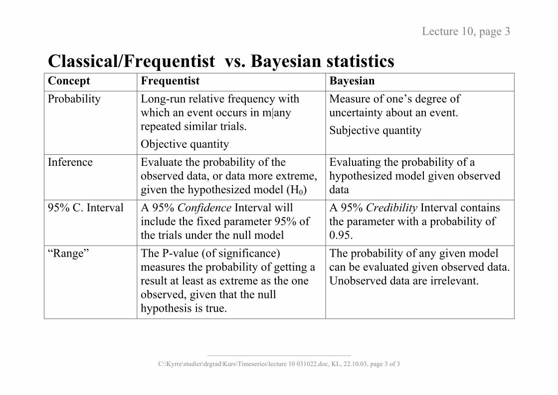
Classical/Frequentist vs. Bayesian statistics Concept Frequentist Bayesian

Probability Long-run relative frequency with which an event occurs in m|any repeated similar trials. Objective quantity

Measure of one’s degree of uncertainty about an event. Subjective quantity

Inference Evaluate the probability of the observed data, or data more extreme, given the hypothesized model (H0)

Evaluating the probability of a hypothesized model given observed data

95% C. Interval A 95% Confidence Interval will include the fixed parameter 95% of the trials under the null model

A 95% Credibility Interval contains the parameter with a probability of 0.95.

“Range” The P-value (of significance) measures the probability of getting a result at least as extreme as the one observed, given that the null hypothesis is true.

The probability of any given model can be evaluated given observed data. Unobserved data are irrelevant.

___________________________________________


Lecture 10, page 4

Formal framework of Bayesian Statistics Bayes’s theorem (entirely uncontroversial) states that the probability that event A occurs, given that event B has occurred, is equal to the probability that both A and B occur, divided by the probability of the occurrence of B:

)()()(

BPBAPBAP ∩

=

Now setting A as a parameter, a collection of parameters, i.e., the hypothesis (θ ) and B as the obtained data (x):

)()()|(

)()()(

xPPxP

xPxPxP θθθθ x

=∩

=

P(θ|x) is the Posterior (probability) of obtaining a parameter estimate θ, given the data obtained. P(x|θ) is the likelihood of obtaining the data under the hypothesis (the same quantity as in frequentist statistics) P(θ) is the Prior probability of θ P(x) is the probability of obtaining the data under all admissible parameter estimates (essentially a scaling constant)

“Posterior = prior x likelihood”

___________________________________________


Lecture 10, page 5

Mighty Joe and Herman

– An example

0.3

0.2

0.1

0.4

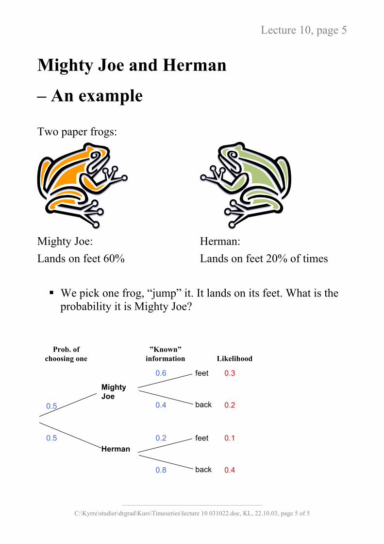
Two paper frogs:

Mighty Joe: Herman: Lands on feet 60% Lands on feet 20% of times We pick one frog, “jump” it. It lands on its feet. What is the

probability it is Mighty Joe?

Mighty Joe

Herman

feet

back

0.6

0.4

feet

back

0.2

0.8

0.5

0.5

Prob. of choosing one

”Known” information

Likelihood

___________________________________________


Lecture 10, page 6

We frame this in the Bayesian setting:

)()()(

BPBAPBAP ∩

= , and in our example:

75.01.03.0

3.0)(

)()( =+

=∩

=feetP

feetJoePfeetJoeP

Thus, the probability that this was Mighty Joe is 75%. We “jump” the frog again. Again it lands on its feet. How

can we Update our belief whether or not this is Mighty Joe?

Mighty Joe

Herman

feet

back

0.6

0.4

feet

back

0.2

0.8

0.75

0.25

Revised Prob. of choosing one (i.e. the prior)


Revised Likelihood

0.45

0.30

0.05

0.20

90.005.045.0

45.0)(

)()( =+

=∩

=feetP

feetJoePfeetJoeP

___________________________________________


Lecture 10, page 7

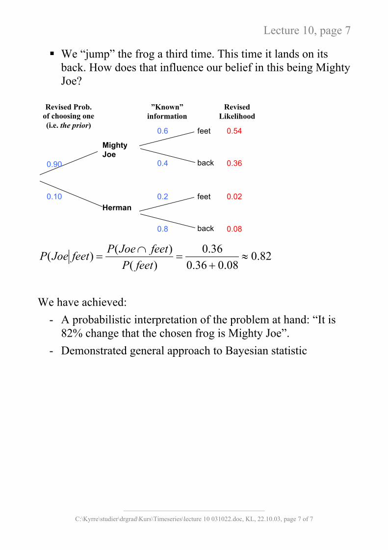
We “jump” the frog a third time. This time it lands on its back. How does that influence our belief in this being Mighty Joe?

Mighty Joe

Herman

feet

back

0.6

0.4

feet

back

0.2

0.8

0.90

0.10

Revised Prob. of choosing one (i.e. the prior)


Revised Likelihood

0.54

0.36

0.02

0.08

82.008.036.0

36.0)(

)()( ≈+

=∩

=feetP

feetJoePfeetJoeP

We have achieved:

- A probabilistic interpretation of the problem at hand: “It is 82% change that the chosen frog is Mighty Joe”.

- Demonstrated general approach to Bayesian statistic

___________________________________________


Lecture 10, page 8

General approach in Bayesian statistics: Use available information to develop a prior. Get new data Find posterior Update prior Get new data

This is an appealing framework of statistics. Is this why we should become Bayesian? Not really – My reason is pragmatic, and it involves a short detour to state-space models.

___________________________________________


Lecture 10, page 9

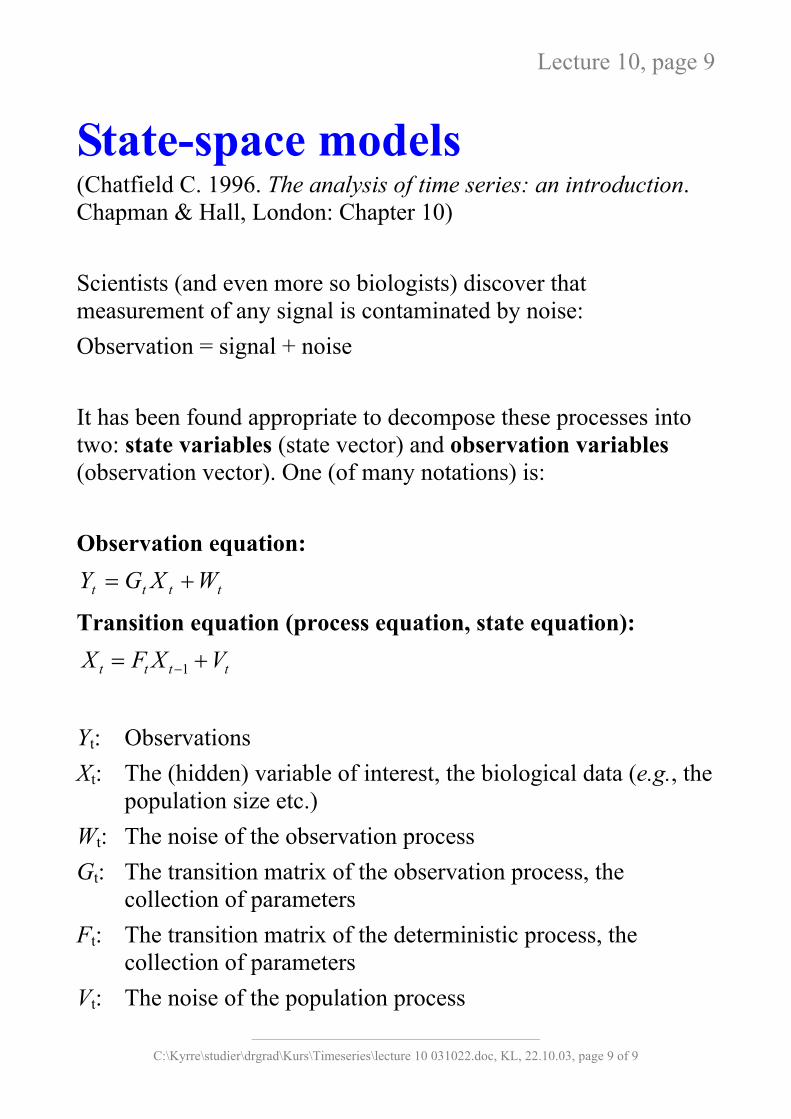
State-space models (Chatfield C. 1996. The analysis of time series: an introduction. Chapman & Hall, London: Chapter 10) Scientists (and even more so biologists) discover that measurement of any signal is contaminated by noise: Observation = signal + noise It has been found appropriate to decompose these processes into two: state variables (state vector) and observation variables (observation vector). One (of many notations) is: Observation equation:

tttt WXGY += Transition equation (process equation, state equation):

tttt VXFX += −1 Yt: Observations Xt: The (hidden) variable of interest, the biological data (e.g., the

population size etc.) Wt: The noise of the observation process Gt: The transition matrix of the observation process, the

collection of parameters Ft: The transition matrix of the deterministic process, the

collection of parameters Vt: The noise of the population process

___________________________________________


Lecture 10, page 10

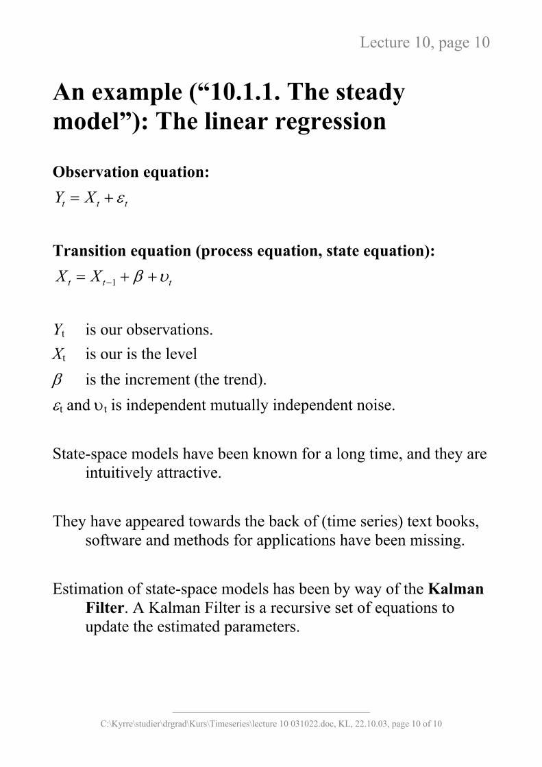
An example (“10.1.1. The steady model”): The linear regression Observation equation:

ttt XY ε+= Transition equation (process equation, state equation):

ttt XX υβ ++= −1 Yt is our observations. Xt is our is the level β is the increment (the trend). εt and υt is independent mutually independent noise. State-space models have been known for a long time, and they are

intuitively attractive. They have appeared towards the back of (time series) text books,

software and methods for applications have been missing. Estimation of state-space models has been by way of the Kalman

Filter. A Kalman Filter is a recursive set of equations to update the estimated parameters.

___________________________________________


Lecture 10, page 11

We see that the idea of updating in the Kalman Filter is related to the Bayesian approach described earlier. Indeed, the theory behind the Kalman Filter is Bayesian.

Until recently, it has been very challenging to actually perform the

Kalman Filter procedure. Now, increased computational power and software (i.e., BUGS)

have made it possible for a wide variety of scientist to estimate state-space models.

___________________________________________


Lecture 10, page 12

Known vs. Unknown distribution (=> Likelihood) If we can assume that the likelihood is known, i.e., that it can be

written out, the recursive equations can be explicitly calculated.

Example: Airpass.dat The number of air passengers can be expressed as a growth model

(the upper equation is the observation model):

21

111

ttt

tttt

tttY

ω+β=βω+β+µ=µ

ν+µ=

−

−−

where Yt is the observed nuµt is the level βt is the growth/increment iνt, ωt1 and ωt2 is independenIn addition the seasonal com These equations have been on West M. & Harrison J. 1dynamic models. Springer,

_____________

C:\Kyrre\studier\drgrad\Kurs\Times

Observation equation
State equations
mber of passengers,

n passenger level (allowed to vary). t mutually independent noise. ponent is removed.

fitted by the splus codes “bts” based 997. Bayesian forecasting and New York.

______________________________

eries\lecture 10 031022.doc, KL, 22.10.03, page 12 of 12

Lecture 10, page 13

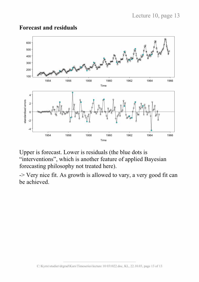
Forecast and residuals

Time

1954 1956 1958 1960 1962 1964 1966100

200

300

400

500

600

Time

stan

dard

ised

erro

rs

1954 1956 1958 1960 1962 1964 1966

-4

-2

0

2

4

Upper is forecast. Lower is residuals (the blue dots is “interventions”, which is another feature of applied Bayesian forecasting philosophy not treated here). -> Very nice fit. As growth is allowed to vary, a very good fit can be achieved.

___________________________________________


Lecture 10, page 14

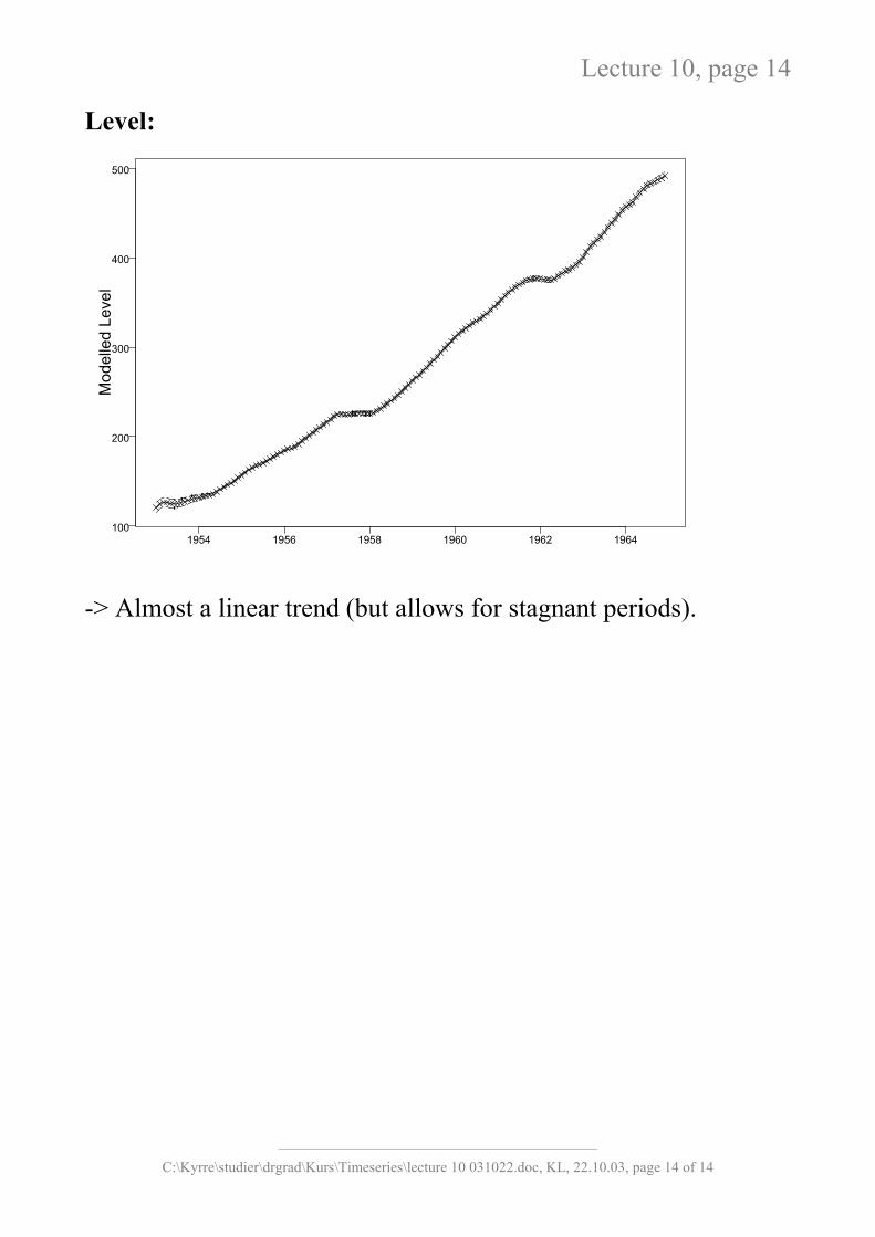
Level:

1954 1956 1958 1960 1962 1964100

200

300

400

500

Mod

elle

d Le

vel

-> Almost a linear trend (but allows for stagnant periods).

___________________________________________


Lecture 10, page 15

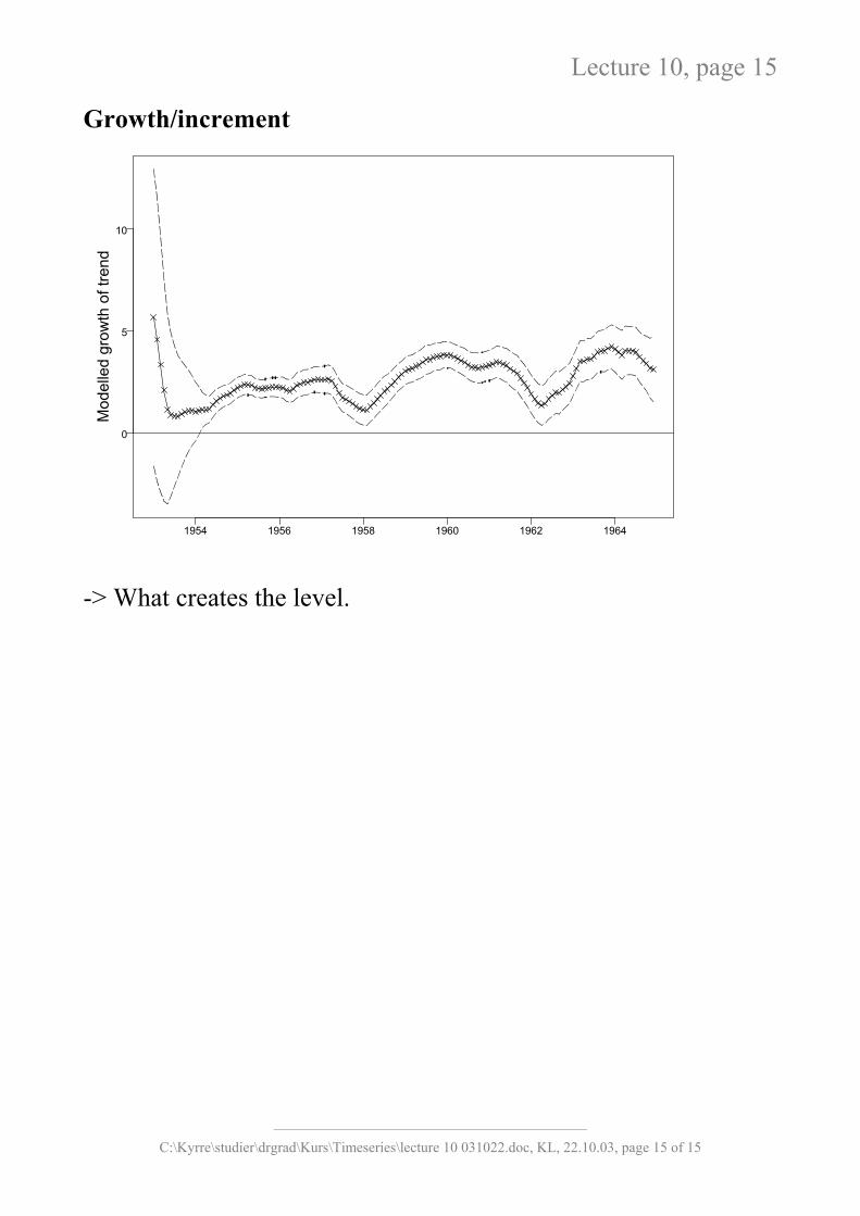
Growth/increment

1954 1956 1958 1960 1962 1964

0

5

10

Mod

elle

d gr

owth

of t

rend

-> What creates the level.

___________________________________________


Lecture 10, page 16

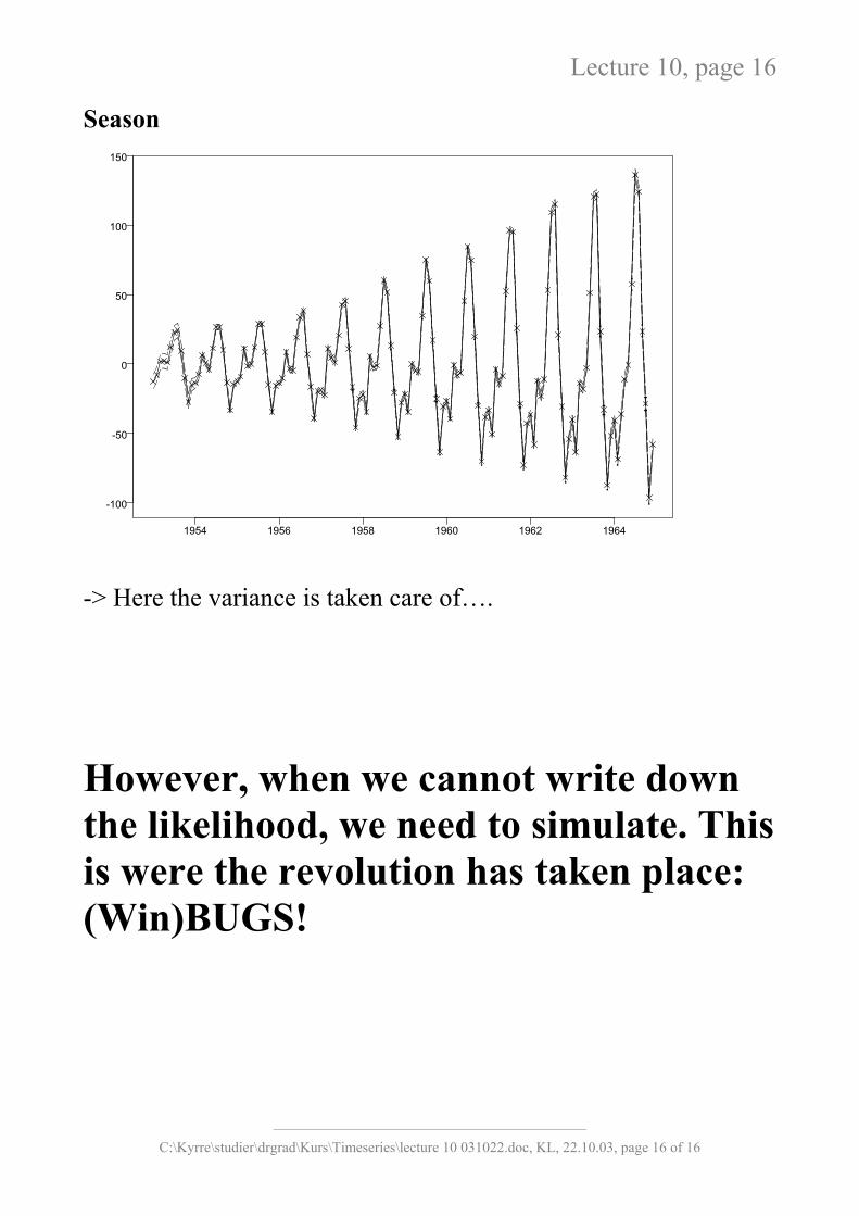
Season

1954 1956 1958 1960 1962 1964

-100

-50

0

50

100

150

-> Here the variance is taken care of….

However, when we cannot write down the likelihood, we need to simulate. This is were the revolution has taken place: (Win)BUGS!

___________________________________________


Lecture 10, page 17

BUGS and time series modelling (Bayesian inference Using Gibbs Sampling) Freely available: http://www.mrc-bsu.cam.ac.uk/bugs/welcome.shtml A program package for simulation of data, using certain

schemes (“Gibbs” and “Metropolis-Hastings”) to sample from distributions. Using the simulated data to draw inference of the parameters, given the data Taking advantage of the Markov Chain property (i.e., a set

up in which all information up to time t is contained in the information for time t-1). Using the Monte Carlo principle2 to obtain non-random

information (“Integration”) If the distribution is known, BUGS is not necessary (the

problem could also be solved by, e.g., maximum likelihood methods). However, the results will be overall in agreement. If the distribution is not correctly specified using ml-

methods, simulation may lead to a different (an probably more correct) result. Complex likelihoods can be specified

2 The method is called after the city in the Monaco principality, because of roulette, a simple random number generator. The term 'Monte Carlo' was introduced by von Neumann and Ulam during World War II, as a code word for the secret work at Los Alamos (M. Kittilsen, pers.com)

___________________________________________


http://www.mrc-bsu.cam.ac.uk/bugs/welcome.shtml

http://www.mrc-bsu.cam.ac.uk/bugs/welcome.shtml

Lecture 10, page 18

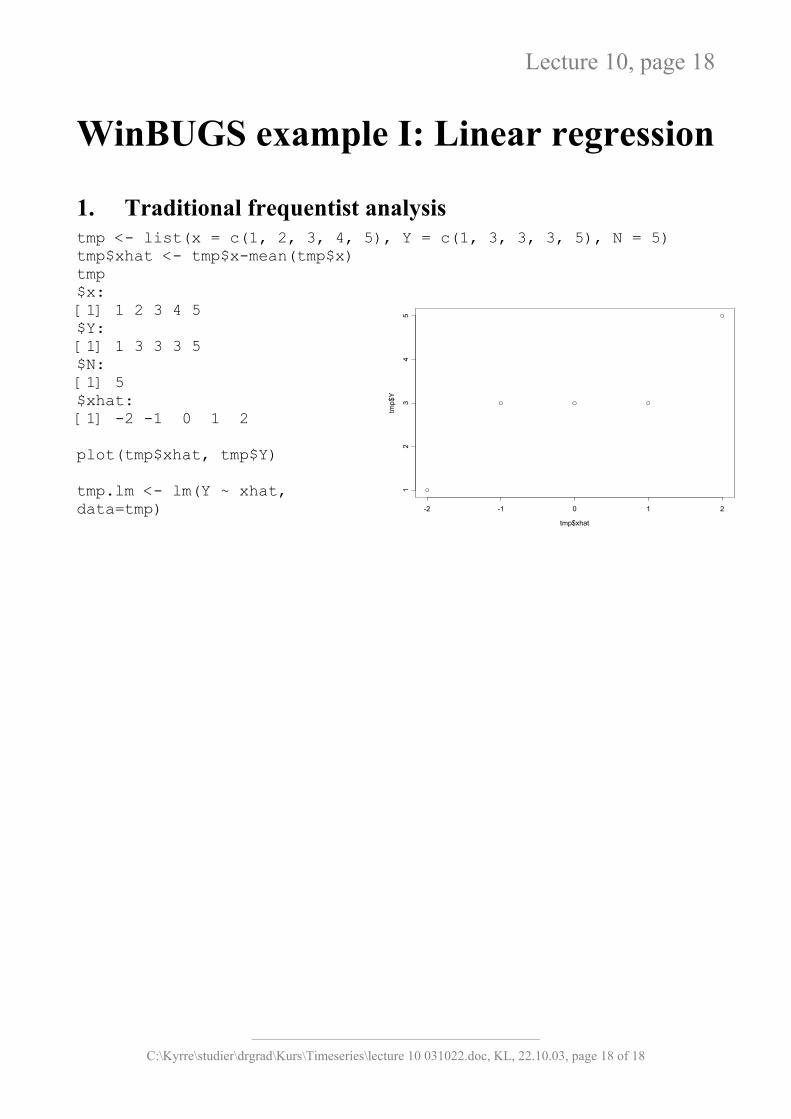
WinBUGS example I: Linear regression 1. Traditional frequentist analysis tmp <- list(x = c(1, 2, 3, 4, 5), Y = c(1, 3, 3, 3, 5), N = 5) tmp$xhat <- tmp$x-mean(tmp$x) tmp

tmp$xhat

tmp$

Y

-2 -1 0 1 2

12

34

5

$x: [1] 1 2 3 4 5 $Y: [1] 1 3 3 3 5 $N: [1] 5 $xhat: [1] -2 -1 0 1 2 plot(tmp$xhat, tmp$Y) tmp.lm <- lm(Y ~ xhat, data=tmp)

___________________________________________


Lecture 10, page 19

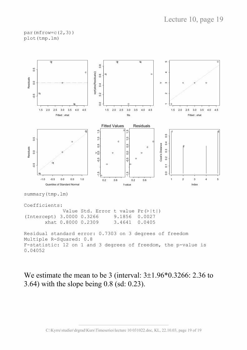
par(mfrow=c(2,3)) plot(tmp.lm)

Fitted : xhat

Res

idua

ls

1.5 2.0 2.5 3.0 3.5 4.0 4.5

-0.5

0.0

0.5

1

4

2

fits

sqrt(

abs(

Res

idua

ls))

1.5 2.0 2.5 3.0 3.5 4.0 4.5

0.0

0.2

0.4

0.6

0.8

1

42

Fitted : xhat

Y

1.5 2.0 2.5 3.0 3.5 4.0 4.5

12

34

5

Quantiles of Standard Normal

Res

idua

ls

-1.0 -0.5 0.0 0.5 1.0

-0.5

0.0

0.5

1

4

2

Fitted Values

0.2 0.6

-1.5

-0.5

0.0

0.5

1.0

1.5

Residuals

0.2 0.6

-1.5

-0.5

0.0

0.5

1.0

1.5

f-value

Y

Index

Coo

k's

Dis

tanc

e

1 2 3 4 5

0.0

0.1

0.2

0.3

0.4

0.5

2

51

summary(tmp.lm) Coefficients: Value Std. Error t value Pr(>|t|) (Intercept) 3.0000 0.3266 9.1856 0.0027 xhat 0.8000 0.2309 3.4641 0.0405 Residual standard error: 0.7303 on 3 degrees of freedom Multiple R-Squared: 0.8 F-statistic: 12 on 1 and 3 degrees of freedom, the p-value is 0.04052

We estimate the mean to be 3 (interval: 3±1.96*0.3266: 2.36 to 3.64) with the slope being 0.8 (sd: 0.23).

___________________________________________


Lecture 10, page 20

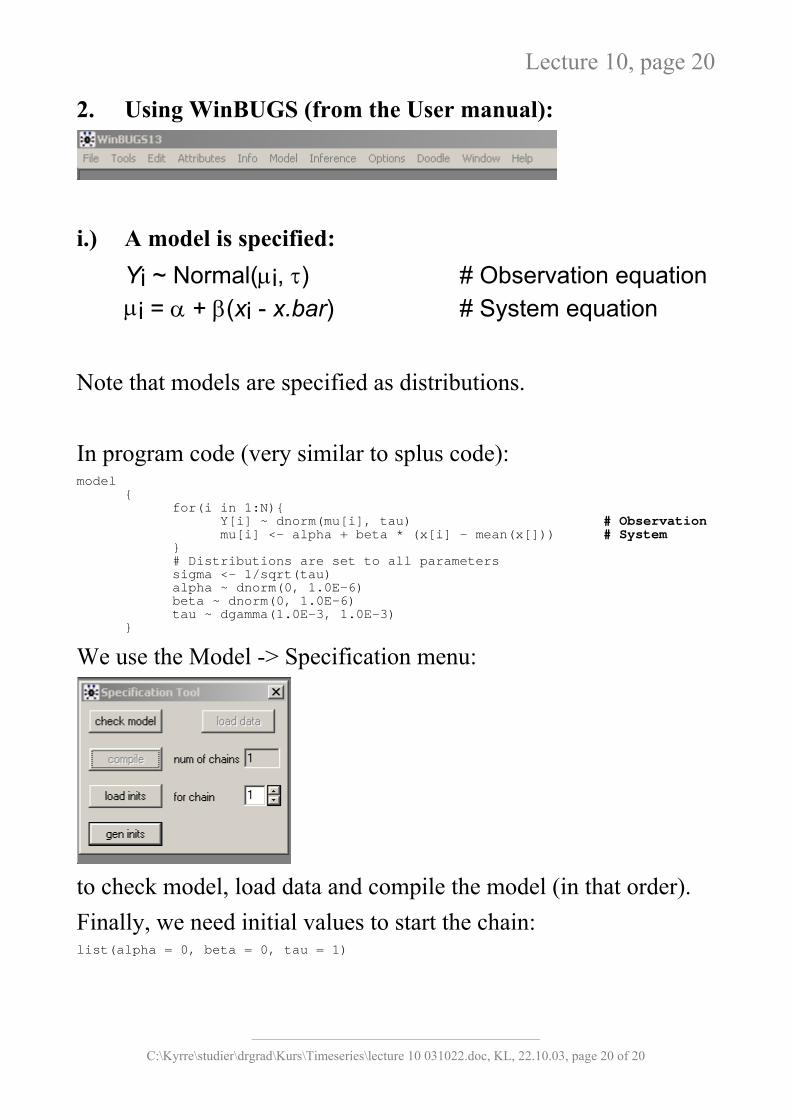
2. Using WinBUGS (from the User manual):

i.) A model is specified:

Yi ~ Normal(µi, τ) # Observation equation µi = α + β(xi - x.bar) # System equation

Note that models are specified as distributions. In program code (very similar to splus code): model { for(i in 1:N){ Y[i] ~ dnorm(mu[i], tau) # Observation mu[i] <- alpha + beta * (x[i] - mean(x[])) # System }

# Distributions are set to all parameters sigma <- 1/sqrt(tau) alpha ~ dnorm(0, 1.0E-6) beta ~ dnorm(0, 1.0E-6) tau ~ dgamma(1.0E-3, 1.0E-3) } We use the Model -> Specification menu:

to check model, load data and compile the model (in that order). Finally, we need initial values to start the chain: list(alpha = 0, beta = 0, tau = 1)

___________________________________________


Lecture 10, page 21

ii). We are now ready to set monitoring scheme This is done in the Inference -> Sample Monitor Tool. Here we decide what parameters to save and monitor:

(we sample alpha, beta, tau and sigma – all variables, finish with a ‘*’).

- Then we click “trace” to see the development iii.) We are ready to sample from the distributions specified

- We take 11.000 samples (and let the 1000 first be ‘burn-in’, i.e., to stabilise the values somewhat) These are the results:

___________________________________________


Lecture 10, page 22

___________________________________________


Lecture 10, page 23

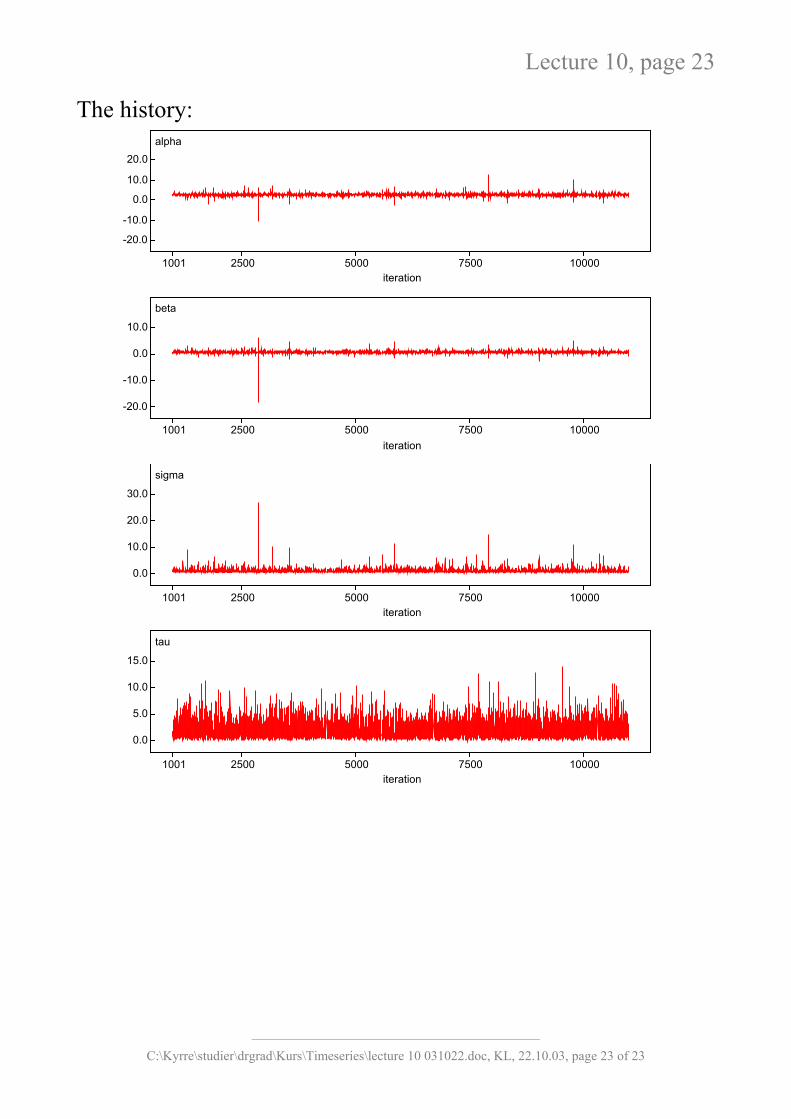
The history: alpha

iteration1001 2500 5000 7500 10000

-20.0

-10.0

0.0

10.0

20.0

beta

iteration1001 2500 5000 7500 10000

-20.0

-10.0

0.0

10.0

sigma

iteration1001 2500 5000 7500 10000

0.0

10.0

20.0

30.0

tau

iteration1001 2500 5000 7500 10000

0.0

5.0

10.0

15.0

___________________________________________


Lecture 10, page 24

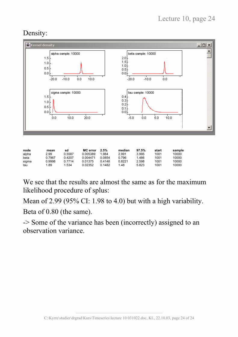
Density:

node mean sd MC error 2.5% median 97.5% start sample alpha 2.99 0.5587 0.005389 1.984 2.991 3.995 1001 10000 beta 0.7967 0.4207 0.004471 0.0854 0.796 1.486 1001 10000 sigma 0.9998 0.7714 0.01375 0.4148 0.8221 2.598 1001 10000 tau 1.89 1.534 0.02352 0.1482 1.48 5.823 1001 10000

We see that the results are almost the same as for the maximum likelihood procedure of splus: Mean of 2.99 (95% CI: 1.98 to 4.0) but with a high variability. Beta of 0.80 (the same). -> Some of the variance has been (incorrectly) assigned to an observation variance.

___________________________________________


Lecture 10, page 25

WinBUGS example II: Community dynamics in the coastal zone Model:

11* tt

Ttt brsas εω +++= − (ib)

where st-1 = log(St-1). a is autoregressive parameter, b is environmental coefficients, ω is environmental data.

1tε is assumed to be normally distributed with expectation zero and

some variance, say . This is equivalent to writing: 2σ

),*(~ 11 tt

Ttt brsbNs εω++− (ib)

This is the system equation/state equation/process equation. We furthermore formulate an observation model:

2}exp{ ttt sS ε+= (iia) which can be reformulated as the following.

)},(exp{~ 2ttt sNS ε (iia)

where ε is given by the estimated standard errors found in Lekve K., Boulinier T., Stenseth N.C., Gjøsæter J., Fromentin J.-M., Hines J.E. & Nichols J.D. 2002. Spatio-temporal dynamics of species richness in coastal fish communities. Proc. R. Soc. Lond. B, 269, 1781-1789.

2t

___________________________________________


Lecture 10, page 26

In BUGS language, this is the following # model with environment in process model: “C:\Kyrre\Studier\Cr\SPMOD\Oecologia\Oecol2nd\OecBug\armodel1b” model

{

s[1] ~ dnorm(0, var);

for (i in 2:N)

{

muS[i] <- r + b * s[i-1]+ psi*naot1[i] +tau*temp[i]+rho*wind[i] # Observation equation s[i] ~ dnorm(muS[i], var) # System equation for first obs. }

for (i in 1:N)

{

Shat[i] ~ dnorm(ant[i], estvar[i])I(0,) # System equation for next obs. log(ant[i]) <- s[i]

}

# Putting distributions on all parameters r~dnorm(0,0.000001)

sd <- 1/sqrt(var)

var~dgamma(0.001,0.001)

b ~ dnorm(0,0.0001)

psi ~ dnorm(0,0.0001)

tau ~ dnorm(0,0.0001)

rho ~ dnorm(0,0.0001)

a <- 1-b

R0 <- exp(r)

for (i in 1:N)

{

S[i] <- exp(s[i])

}

meanS <- mean(S[])

}

# Data (Kragerø) # Initialising values (two files)

___________________________________________


Lecture 10, page 27 list(var = 6, psi = 1, tau=0.5, rho=1, b = 1, r=1,

s = c(1,1,1,1,1,1,1,1,1,1,1,1,1,1,1,1,1,1,1,1,1,1,1,1,1,1,1,1,1,1,1,1,1,1,1,1,1,1))

list(var = 2, psi = 0.5, tau=1, rho=0.5, b=0.2, r=0.5,

s = c(0,0,0,0,0,0,0,0,0,0,0,0,0,0,0,0,0,0,0,0,0,0,0,0,0,0,0,0,0,0,0,0,0,0,0,0,0,0))

-> Using two chains: 110.000 iterations (time two chains: starting on 60.001): Thinning every 10. simulation => sample size of 10.000

Selected results:

node mean sd MC error 5.0% median 95.0% start sample

R0 7.915 9.062 0.3297 1.477 5.561 21.69 60001 10000

a 0.6226 0.297 0.01095 0.1415 0.6212 1.12 60001 10000

meanS 16.66 0.1049 0.001064 16.49 16.66 16.83 60001 10000

psi 0.08219 0.1143 0.001159 -0.1044 0.08236 0.2698 60001 10000

rho 0.1977 0.1337 0.001453 -0.0187 0.1977 0.4194 60001 10000

sd 0.5879 0.07516 8.095E-4 0.4777 0.5817 0.7232 60001 10000

tau -0.1557 0.1438 0.001589 -0.3915 -0.1567 0.08139 60001 10000

___________________________________________


Lecture 10, page 28

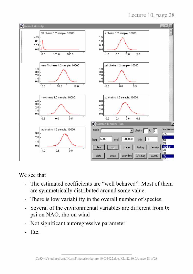
We see that

- The estimated coefficients are “well behaved”: Most of them are symmetrically distributed around some value.

- There is low variability in the overall number of species. - Several of the environmental variables are different from 0:

psi on NAO, rho on wind - Not significant autoregressive parameter - Etc.

___________________________________________


Lecture 10, page 29

___________________________________________


Assessment A Bayesian approach • Appealing concepts of probability etc. • Useful for estimating both observation and system variability

(much due software advances) • Very useful for complex problems with not known distributions

(e.g., in DNA-analysis) • Known likelihoods => Recursions can be explicitly determined

(e.g., BTS) • Unknown likelihoods => Simulation (BUGS)

Documents

Lecture 10: Bayesian modelling of time series - uio.no · model”): The linear regression Observation equation: Yt =Xt +εt Transition equation (process equation, state equation):