Multiperiod Planning and Covering Models

University of ChicagoGraduate School of Business

Introduction to Computer Based Models Bus-36102-81Mr. Schrage Spring 2003

Distinctive Features of Multiperiod Planning:

Decisions made in one period affect results in other periods.

Applications: Demand and Capacity Planning;

How to represent?

Inventory variable(s) tie one-period models together.

The inventory equation:

Beginning inventory + production

= demand + ending inventory;

Symbolically:

It-1 + Pt = Dt + It ;

If there is attrition or growth:

g* It-1 + Pt = Dt + It ;

Key Ideas to Note:

Inventory variable;

Representing financial features:

Generalization of Net Present Value to

different rates for

different periods,

different maturities,

borrowing vs. lending

borrowing small amount vs. large;

Representing taxes;

Cash Flow Matching Portfolio

Situation:

We are faced with a stream of future cash requirements.

We want to set aside a lump sum now to guarantee ability to match these requirements.

Examples:

Lump sum settlements in come personal injury liability cases.

Removing debt from a balance sheet in so-called defeasance.

Trust fund for college education.

Fund to pay off lottery winners.

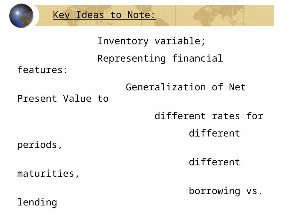
Approaches:

a) Compute present value of the stream.

Q. What is appropriate interest rate?

Injured party wants _________

Paying party wants _________

b) Buy a collection of high quality bonds so that cash throw-offs satisfy cash needs.

If consider more than just zero-coupon bonds, then this is an LP.

Example:

Bond 1 Bond 2

Price: 980 965

Matures(yrs): 5 12

Rate/yr: 6% 6.5%

MODEL: MIN = L; [P00] L - .98 * B1 - .965 * B2 >= 10; [P01] .06 * B1 + .065 * B2 >= 11; [P02] .06 * B1 + .065 * B2 >= 12; [P03] .06 * B1 + .065 * B2 >= 14; [P04] .06 * B1 + .065 * B2 >= 15; [P05] 1.06 * B1 + .065 * B2 >= 17; [P06] .065 * B2 >= 19; [P07] .065 * B2 >= 20; [P08] .065 * B2 >= 22; [P09] .065 * B2 >= 24; [P10] .065 * B2 >= 26; [P11] .065 * B2 >= 29; [P12] 1.065 * B2 >= 31;END

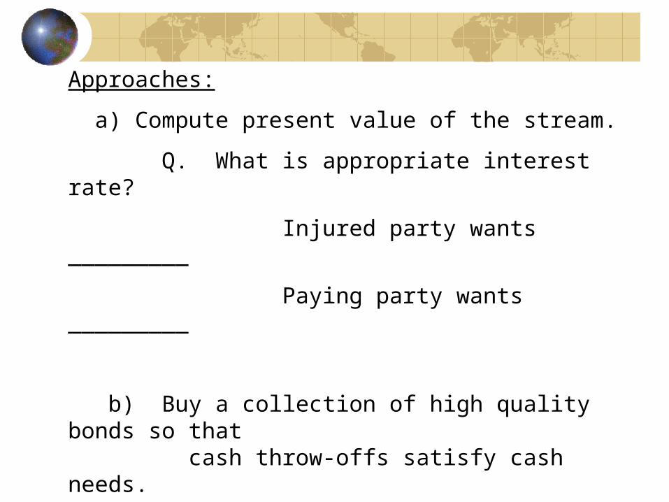
What is a Q&D estimate of the lump sum, L?

Variable Value Reduced Cost L 440.5385 0.0000000 B1 0.0000000 0.9800000 B2 446.1538 0.0000000

Row Slack or Surplus Dual Price 1 440.5385 1.000000 P00 0.0000000 -1.000000 P01 18.00000 0.0000000 P02 17.00000 0.0000000 P03 15.00000 0.0000000 P04 14.00000 0.0000000 P05 12.00000 0.0000000 P06 10.00000 0.0000000 P07 9.000000 0.0000000 P08 7.000000 0.0000000 P09 5.000000 0.0000000 P10 3.000000 0.0000000 P11 0.0000000 -14.84615 P12 444.1538 0.0000000

Hmm, takes a lot of money! What are we missing?

MODEL: MIN = L; [P00] L - .98 * B1 - .965 * B2 - S0 = 10; [P01] .06 * B1 + .065 * B2 + 1.04 * S0 - S1 = 11; [P02] .06 * B1 + .065 * B2 + 1.04 * S1 - S2 = 12; [P03] .06 * B1 + .065 * B2 + 1.04 * S2 - S3 = 14; [P04] .06 * B1 + .065 * B2 + 1.04 * S3 - S4 = 15; [P05] 1.06 * B1 + .065 * B2 + 1.04 * S4 - S5 = 17; [P06] .065 * B2 + 1.04 * S5 - S6 = 19; [P07] .065 * B2 + 1.04 * S6 - S7 = 20; [P08] .065 * B2 + 1.04 * S7 - S8 = 22; [P09] .065 * B2 + 1.04 * S8 - S9 = 24; [P10] .065 * B2 + 1.04 * S9 - S10 = 26; [P11] .065 * B2 + 1.04 * S10 - S11 = 29; [P12] 1.065 * B2 + 1.04 * S11 - S12 = 31;END

Add opportunity to invest for one period, each period:

Variable Value Reduced Cost L 168.98760 0.0000000 B1 119.16280 0.0000000 B2 29.10798 0.0000000 S0 14.11887 0.0000000 S1 12.72541 0.0000000 S2 10.27622 0.0000000 S3 5.72905 0.0000000 S4 0.00000 0.1069792 S5 111.20460 0.0000000 S6 98.54478 0.0000000 S7 84.37859 0.0000000 S8 67.64575 0.0000000 S9 48.24360 0.0000000 S10 26.06537 0.0000000 S11 0.00000 0.1412458 S12 0.00000 0.4106152

Row Slack or Surplus Dual Price 1 168.9876 1.000000 P00 0.0000000 -1.000000 P01 0.0000000 -0.9615384 P02 0.0000000 -0.9245562 P03 0.0000000 -0.8889964 P04 0.0000000 -0.8548042 P05 0.0000000 -0.7190625 P06 0.0000000 -0.6914063 P07 0.0000000 -0.6648138 P08 0.0000000 -0.6392440 P09 0.0000000 -0.6146576 P10 0.0000000 -0.5910170 P11 0.0000000 -0.5682856 P12 0.0000000 -0.4106152

What is the interpretation of the dual prices?

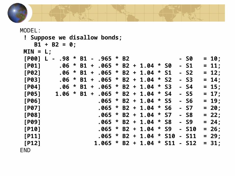
MODEL: ! Suppose we disallow bonds; B1 + B2 = 0; MIN = L; [P00] L - .98 * B1 - .965 * B2 - S0 = 10; [P01] .06 * B1 + .065 * B2 + 1.04 * S0 - S1 = 11; [P02] .06 * B1 + .065 * B2 + 1.04 * S1 - S2 = 12; [P03] .06 * B1 + .065 * B2 + 1.04 * S2 - S3 = 14; [P04] .06 * B1 + .065 * B2 + 1.04 * S3 - S4 = 15; [P05] 1.06 * B1 + .065 * B2 + 1.04 * S4 - S5 = 17; [P06] .065 * B2 + 1.04 * S5 - S6 = 19; [P07] .065 * B2 + 1.04 * S6 - S7 = 20; [P08] .065 * B2 + 1.04 * S7 - S8 = 22; [P09] .065 * B2 + 1.04 * S8 - S9 = 24; [P10] .065 * B2 + 1.04 * S9 - S10 = 26; [P11] .065 * B2 + 1.04 * S10 - S11 = 29; [P12] 1.065 * B2 + 1.04 * S11 - S12 = 31;END

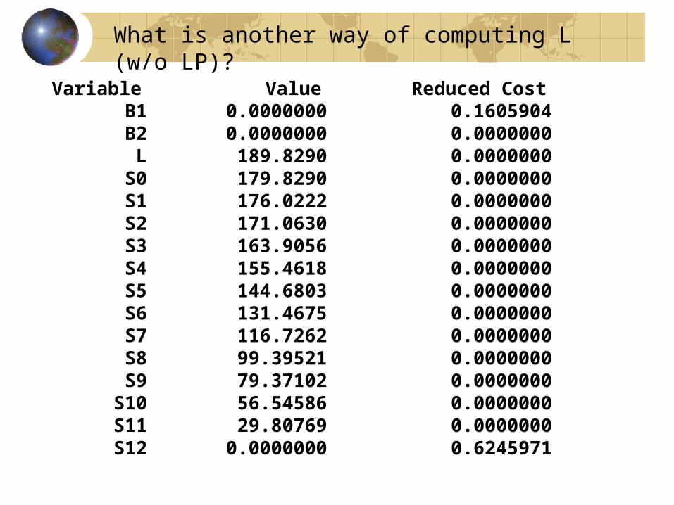
Variable Value Reduced Cost B1 0.0000000 0.1605904 B2 0.0000000 0.0000000 L 189.8290 0.0000000 S0 179.8290 0.0000000 S1 176.0222 0.0000000 S2 171.0630 0.0000000 S3 163.9056 0.0000000 S4 155.4618 0.0000000 S5 144.6803 0.0000000 S6 131.4675 0.0000000 S7 116.7262 0.0000000 S8 99.39521 0.0000000 S9 79.37102 0.0000000 S10 56.54586 0.0000000 S11 29.80769 0.0000000 S12 0.0000000 0.6245971

What is another way of computing L (w/o LP)?

Row Slack or Surplus Dual 1 0.000000 0.2696269 2 189.829000 1.000000P00 0.000000 -1.000000P01 0.000000 -0.9615384P02 0.000000 -0.9245562P03 0.000000 -0.8889964P04 0.000000 -0.8548042P05 0.000000 -0.8219271P06 0.000000 -0.7903146P07 0.000000 -0.7599178P08 0.000000 -0.7306902P09 0.000000 -0.7025867P10 0.000000 -0.6755642P11 0.000000 -0.6495810P12 0.000000 -0.6245971

Is there a simple formula for these dual prices?

MODEL: ! Suppose we can buy only an integer number of bonds. Does it hurt us much?; @GIN( B1); @GIN( B2); MIN = L; [P00] L - .98 * B1 - .965 * B2 - S0 = 10; [P01] .06 * B1 + .065 * B2 + 1.04 * S0 - S1 = 11; [P02] .06 * B1 + .065 * B2 + 1.04 * S1 - S2 = 12; [P03] .06 * B1 + .065 * B2 + 1.04 * S2 - S3 = 14; [P04] .06 * B1 + .065 * B2 + 1.04 * S3 - S4 = 15; [P05] 1.06 * B1 + .065 * B2 + 1.04 * S4 - S5 = 17; [P06] .065 * B2 + 1.04 * S5 - S6 = 19; [P07] .065 * B2 + 1.04 * S6 - S7 = 20; [P08] .065 * B2 + 1.04 * S7 - S8 = 22; [P09] .065 * B2 + 1.04 * S8 - S9 = 24; [P10] .065 * B2 + 1.04 * S9 - S10 = 26; [P11] .065 * B2 + 1.04 * S10 - S11 = 29; [P12] 1.065 * B2 + 1.04 * S11 - S12 = 31;END

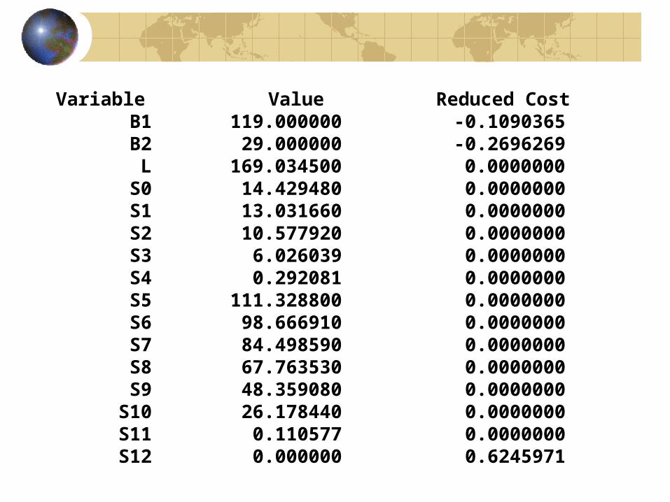
Variable Value Reduced Cost B1 119.000000 -0.1090365 B2 29.000000 -0.2696269 L 169.034500 0.0000000 S0 14.429480 0.0000000 S1 13.031660 0.0000000 S2 10.577920 0.0000000 S3 6.026039 0.0000000 S4 0.292081 0.0000000 S5 111.328800 0.0000000 S6 98.666910 0.0000000 S7 84.498590 0.0000000 S8 67.763530 0.0000000 S9 48.359080 0.0000000 S10 26.178440 0.0000000 S11 0.110577 0.0000000 S12 0.000000 0.6245971

Row Slack or Surplus Dual Price 1 169.0345 1.000000 P00 0.0000000 -1.000000 P01 0.0000000 -0.9615384 P02 0.0000000 -0.9245562 P03 0.0000000 -0.8889964 P04 0.0000000 -0.8548042 P05 0.0000000 -0.8219271 P06 0.0000000 -0.7903146 P07 0.0000000 -0.7599178 P08 0.0000000 -0.7306902 P09 0.0000000 -0.7025867 P10 0.0000000 -0.6755642 P11 0.0000000 -0.6495810 P12 0.0000000 -0.6245971

Other Typical Issues

-Setup costs for producing in a period,

Xt 999 * Yt , Yt = 0 or 1;

-Level change costs:

Changeupt - Changednt = Xt – Xt-1;

-Taxes:

taxt tax_rate * (taxable_revt - taxable_expenset);

sources_of_casht+1 = uses_of_casht+1 + taxt

-End Effects, how to gracefully truncate:

Methods: Limits, salvage values, infinite period.

-NPV vs. LP

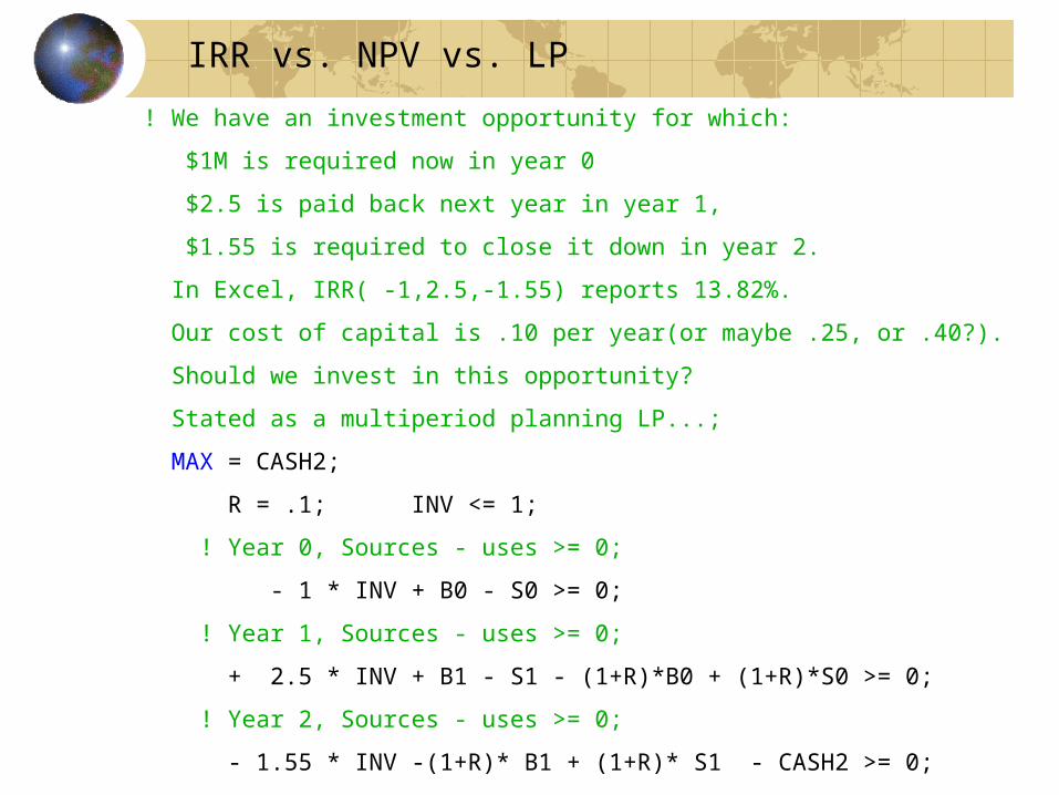
! We have an investment opportunity for which:

$1M is required now in year 0

$2.5 is paid back next year in year 1,

$1.55 is required to close it down in year 2.

In Excel, IRR( -1,2.5,-1.55) reports 13.82%.

Our cost of capital is .10 per year(or maybe .25, or .40?).

Should we invest in this opportunity?

Stated as a multiperiod planning LP...;

MAX = CASH2;

R = .1; INV <= 1;

! Year 0, Sources - uses >= 0;

- 1 * INV + B0 - S0 >= 0;

! Year 1, Sources - uses >= 0;

+ 2.5 * INV + B1 - S1 - (1+R)*B0 + (1+R)*S0 >= 0;

! Year 2, Sources - uses >= 0;

- 1.55 * INV -(1+R)* B1 + (1+R)* S1 - CASH2 >= 0;

IRR vs. NPV vs. LP

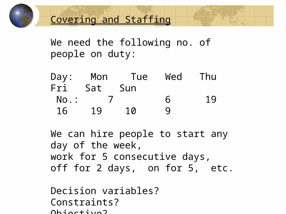
Covering and Staffing We need the following no. of people on duty: Day: Mon Tue Wed Thu Fri Sat Sun No.: 7 6 19 16 19 10 9 We can hire people to start any day of the week,work for 5 consecutive days,off for 2 days, on for 5, etc. Decision variables?Constraints?Objective? 

 

MODEL: MIN = M + T + W + R + F + S + N; [MON] M + R + F + S + N >= 7; [TUE] M + T + F + S + N >= 6; [WED] M + T + W + S + N >= 19; [THU] M + T + W + R + N >= 16; [FRI] M + T + W + R + F >= 19; [SAT] T + W + R + F + S >= 10; [SUN] W + R + F + S + N >= 9; END

If we just minimize number of people hired..

 

Variable Value Reduced Cost M 9.000000 0.000000 T 0.000000 0.000000 W 10.000000 0.000000 R 0.000000 1.000000 F 0.000000 1.000000 S 0.000000 0.000000 N 0.000000 0.000000  Row Slack or Surplus Dual Price 1 19.000000 1.000000 MON 2.000000 0.000000 TUE 3.000000 0.000000 WED 0.000000 -1.000000 THU 3.000000 0.000000 FRI 0.000000 0.000000 SAT 0.000000 0.000000 SUN 1.000000 0.000000 

Any criticisms of this solution?

Suppose overstaffing a given day by up to one person is worth a 0.1 unit of "credit".   MODEL: MIN = M + T + W + R + F + S + N - .1*( EM + ET + EW + ER + EF + ES + EN); [MON] M + R + F + S + N >= 7 + EM; [TUE] M + T + F + S + N >= 6 + ET; [WED] M + T + W + S + N >= 19 + EW; [THU] M + T + W + R + N >= 16 + ER; [FRI] M + T + W + R + F >= 19 + EF; [SAT] T + W + R + F + S >= 10 + ES; [SUN] W + R + F + S + N >= 9 + EN; EM <= 1; ET <= 1; EW <= 1; ER <= 1; EF <= 1; ES <= 1; EN <= 1; END

 

Variable Value Reduced Cost M 8.000000 0.0000000 T 0.000000 0.0000000 W 11.000000 0.0000000 R 0.000000 0.7000000 F 0.000000 0.7000000 S 0.000000 0.0000000 N 0.000000 0.1000000 EM 1.000000 0.0000000 ET 1.000000 0.0000000 EW 0.000000 0.7000000 ER 1.000000 0.0000000 EF 0.000000 0.0000000 ES 1.000000 0.0000000 EN 1.000000 0.0000000

Is this solution any better in some sense?

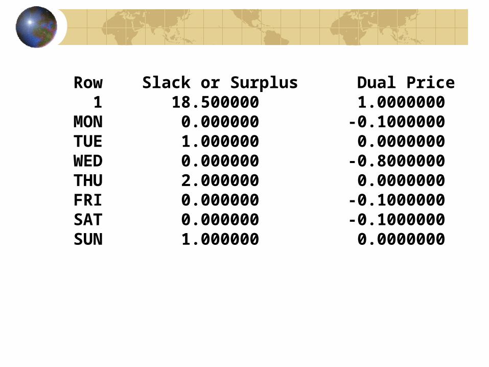
Row Slack or Surplus Dual Price 1 18.500000 1.0000000 MON 0.000000 -0.1000000 TUE 1.000000 0.0000000 WED 0.000000 -0.8000000 THU 2.000000 0.0000000 FRI 0.000000 -0.1000000 SAT 0.000000 -0.1000000 SUN 1.000000 0.0000000 

Demand Planning Multi-period Model

Demand Planning, Promote in November

! Demand planning, (mintendo);SETS: PERIOD: D, W, H, L, P, I, S, C, OV, PRICE;ENDSETSDATA: ! Base case(from Chopra & Meindl); HPU = .25; !Hours to produce one unit; HPM = 160; !Hours/period(month) per employee; HOV = 40; !Lim on Overtime hours/(employee*month); CRM = 12; !Cost of raw material/unit; CI = 4; !Cost of inventory/(unit*period); CS = 10; !Cost of stockout/(unit*period); CH = 3000;!Cost of hiring new employee; CL = 5000;!Cost of laying off an employee; CR = 15; !Cost of regular time/hour; CV = 22.5;!Cost of overtime/hour; CC = 18; !Cost per unit subcontracted; W0 = 300; !Starting workforce size; I0 = 50000;!Starting inventory, < 0 => shortage; PERIOD= JUL AUG SEP OCT NOV DEC; D = 100000 110000 130000 180000 250000 300000; PRICE= 50 50 50 50 50 50;ENDDATA

Demand Planning, LINGO Version

Demand Planning, continued

! Minimize sum of costs of raw materials + inventory + shortage + hiring +layoff +regular time +overtime +subcontracting;MAX = REVENUE - COST;COST = TRM + TIV + TS + THR + TLF + TRT + TOV + TCT;! Compute cost components; TRM = @SUM( PERIOD(T): CRM*P(T)); TIV = @SUM( PERIOD(T): CI*I(T)); TS = @SUM( PERIOD(T): CS*S(T)); THR = @SUM( PERIOD(T): CH*H(T)); TLF = @SUM( PERIOD(T): CL*L(T)); TRT = @SUM( PERIOD(T): CR*HPM*W(T)); TOV = @SUM( PERIOD(T): CV*OV(T)); TCT = @SUM( PERIOD(T): CC*C(T));REVENUE= @SUM( PERIOD(T): PRICE(T)*D(T));

! Constraints for intermediate periods;@FOR (PERIOD(T)| T #GT# 1: !Workforce in T = workforce previous month + hires - layoffs; W(T) = W(T-1) + H(T) - L(T); !Beginning inventory + production + subcontracted production = demand + previous stockouts + inventory -current stockouts; I(T-1) + P(T) + C(T) = D(T) + S(T-1) + I(T) - S(T); P(T) <= (HPM*W(T) + OV(T))/HPU; OV(T) <= HOV*W(T); );! Initial conditions, first period; W(1) = W0 + H(1) - L(1); I0 + P(1) + C(1) = D(1) + I(1) - S(1); P(1) <= (HPM*W(1) + OV(1))/HPU; OV(1) <= HOV*W(1);! Ending conditions; S(@SIZE(PERIOD)) = 0;

Demand Planning, continued.