Embed Size (px)
Citation preview
Applied Mathematics and Computation 170 (2005) 1243–1260
www.elsevier.com/locate/amc
Multiparametric sensitivity analysis ofthe constraint matrix in linear-plus-linear
fractional programming problem
Sanjeet Singh a, Pankaj Gupta b,*, Davinder Bhatia c
a Scientific Analysis Group, DRDO, Ministry of Defence, Metcalfe House, Delhi 110054, Indiab Department of Mathematics, Deen Dayal Upadhyaya College, Shivaji Marg,
Karampura, New Delhi 110015, Indiac Department of Operational Research, University of Delhi, Delhi 110007, India
Abstract
In this paper, we study multiparametric sensitivity analysis for programming prob-
lems with linear-plus-linear fractional objective function using the concept of maximum
volume in the tolerance region. We construct critical regions for simultaneous and inde-
pendent perturbations of one row or one column of the constraint matrix in the given
problem. Necessary and sufficient conditions are given to classify perturbation para-
meters as �focal� and �nonfocal�. Nonfocal parameters can have unlimited variations,because of their low sensitivity in practice, these parameters can be deleted from the
analysis. For focal parameters, a maximum volume tolerance region is characterized.
Theoretical results are illustrated with the help of a numerical example.
� 2005 Elsevier Inc. All rights reserved.
Keywords: Multiparametric sensitivity analysis; Maximum volume region; Generalized fractional
programming; Tolerance approach; Parametric programming
0096-3003/$ - see front matter � 2005 Elsevier Inc. All rights reserved.
doi:10.1016/j.amc.2005.01.016
* Corresponding author.
E-mail addresses: [email protected] (S. Singh), [email protected] (P.
Gupta).
1244 S. Singh et al. / Appl. Math. Comput. 170 (2005) 1243–1260
1. Introduction
A general linear-plus-linear fractional programming problem has the follow-
ing form:
ðLLFPÞ Maximize F ðxÞ ¼ cTxþ pTxqTxþ h
subject to Ax ¼ b;
x P 0;
where A is m · n coefficient matrix with m < n; cT, pT and qT are n-dimensionalrow vectors; x and b are n-dimensional and m-dimensional column vectors
respectively and h is a scalar quantity. It is assumed that the feasible regionof the problem (LLFP) is bounded.
Teterev [14] pointed out that such problems arise when a compromise be-
tween absolute and relative terms is to be maximized. Major applications of
the problem (LLFP) can be found in transportation, problems of optimizingenterprise capital, the production development fund and the social, cultural
and construction fund. Teterev [14] derived an optimality criteria for (LLFP)
using the simplex type algorithm. Several authors studied the problem
(LLFP) and its variants and have discussed their solution properties [2,4,6,
10,11,14].
In practical applications the data collected may not be precise, we would like
to know the effect of data perturbation on the optimal solution. Hence, the
study of sensitivity analysis is of great importance. In general, the main focusof sensitivity analysis is on simultaneous and independent perturbation of the
parameters. Besides this, all the parameters are required to be analyzed at their
independent levels of sensitivity. If one parameter is more sensitive than the
others, the tolerance region characterized by treating all the parameters at
equal levels of sensitivity would be too small for the less sensitive parameters.
If the decision maker has the prior knowledge that some parameters can be
given unlimited variations without affecting the original solution then we con-
sider those parameters as �nonfocal� and these �nonfocal� parameters can be de-leted from the analysis. Wang and Huang [15,16] proposed the concept of
maximum volume in the tolerance region for the multiparametric sensitivity
analysis of a single objective linear programming problem. Their theory allows
the more sensitive parameters called as �focal� to be investigated at their inde-pendent levels of sensitivity, simultaneously and independently. This approach
is a significant improvement over the earlier approaches primarily because be-
sides reducing the number of parameters in the final analysis, it also handles
the perturbation parameters with greater flexibility by allowing them to beinvestigated at their independent levels of sensitivity. Singh et al. [13] extended
the results of Wang and Huang [17] to discuss multiparametric sensitivity
S. Singh et al. / Appl. Math. Comput. 170 (2005) 1243–1260 1245
analysis for changes in the objective function coefficients and the right-hand-
side vector of the problem (LLFP).
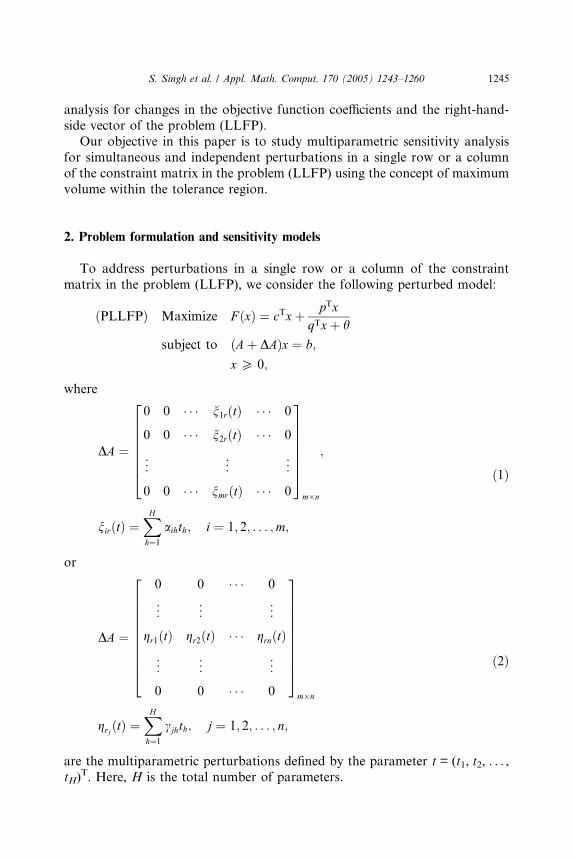
Our objective in this paper is to study multiparametric sensitivity analysis
for simultaneous and independent perturbations in a single row or a column
of the constraint matrix in the problem (LLFP) using the concept of maximum
volume within the tolerance region.
2. Problem formulation and sensitivity models
To address perturbations in a single row or a column of the constraint
matrix in the problem (LLFP), we consider the following perturbed model:
ðPLLFPÞ Maximize F ðxÞ ¼ cTxþ pTxqTxþ h
subject to ðAþ DAÞx ¼ b;
x P 0;
where
DA ¼
0 0 � � � n1rðtÞ � � � 0
0 0 � � � n2rðtÞ � � � 0
..
. ... ..
.
0 0 � � � nmrðtÞ � � � 0
26666664
37777775m�n
;
nirðtÞ ¼XHh¼1
aihth; i ¼ 1; 2; . . . ;m;
ð1Þ
or
DA ¼
0 0 � � � 0
..
. ... ..
.
gr1ðtÞ gr2ðtÞ � � � grnðtÞ
..
. ... ..
.
0 0 � � � 0
26666666664
37777777775m�n
grjðtÞ ¼XHh¼1
cjhth; j ¼ 1; 2; . . . ; n;
ð2Þ
are the multiparametric perturbations defined by the parameter t = (t1, t2, . . . ,tH)
T. Here, H is the total number of parameters.
1246 S. Singh et al. / Appl. Math. Comput. 170 (2005) 1243–1260
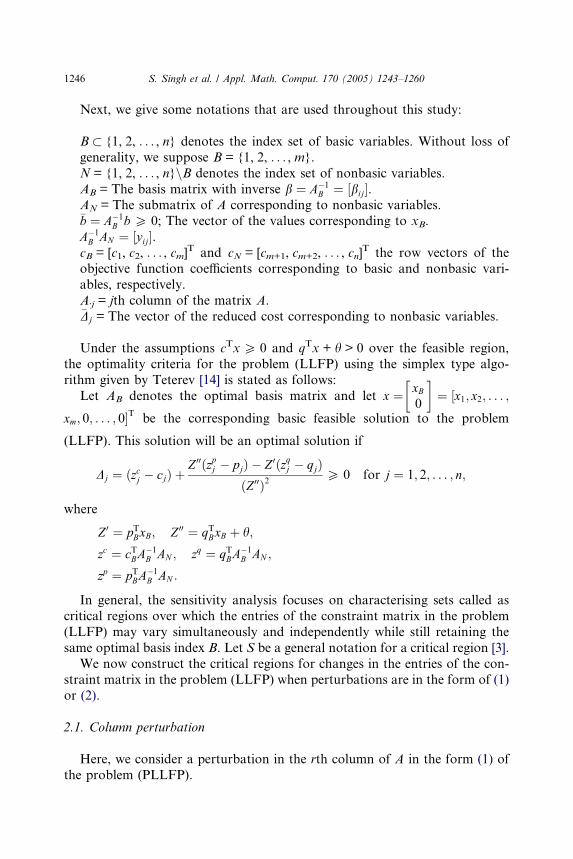
Next, we give some notations that are used throughout this study:
B � {1, 2, . . . , n} denotes the index set of basic variables. Without loss ofgenerality, we suppose B = {1, 2, . . . , m}.N = {1, 2, . . . , n}nB denotes the index set of nonbasic variables.AB = The basis matrix with inverse b ¼ A1
B ¼ ½bij�.AN = The submatrix of A corresponding to nonbasic variables.�b ¼ A1
B b P 0; The vector of the values corresponding to xB.
A1B AN ¼ ½yij�.cB = [c1, c2, . . . , cm]
T and cN = [cm+1, cm+2, . . . , cn]T the row vectors of the
objective function coefficients corresponding to basic and nonbasic vari-
ables, respectively.
AÆj = jth column of the matrix A.�Dj = The vector of the reduced cost corresponding to nonbasic variables.
Under the assumptions cTxP 0 and qTx + h > 0 over the feasible region,the optimality criteria for the problem (LLFP) using the simplex type algo-
rithm given by Teterev [14] is stated as follows:
Let AB denotes the optimal basis matrix and let x ¼ xB0
� ¼ ½x1; x2; . . . ;
xm; 0; . . . ; 0�T be the corresponding basic feasible solution to the problem
(LLFP). This solution will be an optimal solution if
Dj ¼ ðzcj cjÞ þZ 00ðzpj pjÞ Z 0ðzqj qjÞ
ðZ 00Þ2P 0 for j ¼ 1; 2; . . . ; n;
where
Z 0 ¼ pTBxB; Z 00 ¼ qTBxB þ h;
zc ¼ cTBA1B AN ; zq ¼ qTBA
1B AN ;
zp ¼ pTBA1B AN :
In general, the sensitivity analysis focuses on characterising sets called as
critical regions over which the entries of the constraint matrix in the problem
(LLFP) may vary simultaneously and independently while still retaining the
same optimal basis index B. Let S be a general notation for a critical region [3].
We now construct the critical regions for changes in the entries of the con-
straint matrix in the problem (LLFP) when perturbations are in the form of (1)or (2).
2.1. Column perturbation
Here, we consider a perturbation in the rth column of A in the form (1) of
the problem (PLLFP).
S. Singh et al. / Appl. Math. Comput. 170 (2005) 1243–1260 1247
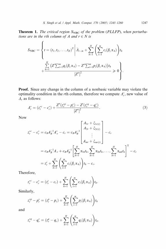
Theorem 1. The critical region SNBC of the problem (PLLFP), when perturba-
tions are in the rth column of A and r 2 N is
SNBC ¼ t ¼ ðt1; t2; . . . ; tHÞT �Drm þXHh¼1
Xmi¼1
ciðbi�a�hÞ !
th
�����8>><>>:
þ
PHh¼1
Z 0Pmi¼1qiðbi�a�hÞ Z 00Pm
i¼1piðbi�a�hÞ� �
th
½Z 00�2P 0
9>>=>>;:
Proof. Since any change in the column of a nonbasic variable may violate the
optimality condition in the rth column, therefore we compute D�r , new value of
Dr as follows:
D�r ¼ ðz�cr c�r Þ þ
Z 00ðz�pr p�r Þ Z 0ðz�qr q�r Þ½Z 00�2
: ð3Þ
Now
z�cr c�r ¼ cBA1B A�
�r cr ¼ cBA1B
A1r þ n1rðtÞA2r þ n2rðtÞ
..
.
Amr þ nmrðtÞ
266664
377775 cr
¼ cBA1B A�r þ cBA
1B
XHh¼1
a1hth;XHh¼1
a2hth; . . . ;XHh¼1
amhth
" #T cr
¼ zcr þXHh¼1
Xmi¼1
ciðbi�a�hÞ !
th cr:
Therefore,
z�cr c�r ¼ ðzcr crÞ þXHh¼1
Xmi¼1
ciðbi�a�hÞ !
th:
Similarly,
z�pr p�r ¼ ðzpr prÞ þXHh¼1
Xmi¼1
piðbi�a�hÞ !
th
and
z�qr q�r ¼ ðzqr qrÞ þXHh¼1
Xmi¼1
qiðbi�a�hÞ !
th:
1248 S. Singh et al. / Appl. Math. Comput. 170 (2005) 1243–1260
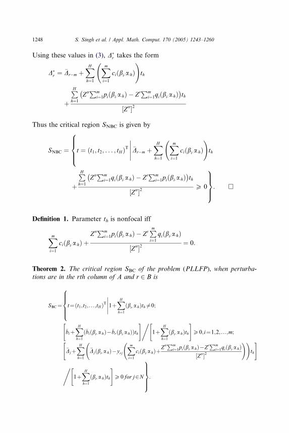
Using these values in (3), D�r takes the form
D�r ¼ �Drm þ
XHh¼1
Xmi¼1
ciðbi�a�hÞ !
th
þ
PHh¼1
Z 00Pmi¼1piðbi�a�hÞ Z 0Pm
i¼1qiðbi�a�hÞ� �
th
½Z 00�2
Thus the critical region SNBC is given by
SNBC ¼ t ¼ ðt1; t2; . . . ; tHÞT �Drm þXHh¼1
Xmi¼1
ciðbi�a�hÞ !
th
�����8>><>>:
þ
PHh¼1
Z 00Pmi¼1qiðbi�a�hÞ Z 0Pm
i¼1piðbi�a�hÞ� �
th
½Z 00�2P 0
9>>=>>;: �
Definition 1. Parameter th is nonfocal iff
Xmi¼1
ciðbi�a�hÞ þZ 00Pm
i¼1piðbi�a�hÞ Z 0Pmi¼1
qiðbi�a�hÞ
½Z 00�2¼ 0:
Theorem 2. The critical region SBC of the problem (PLLFP), when perturba-
tions are in the rth column of A and r 2 B is
SBC¼ t¼ðt1;t2;...;tH ÞT 1þXHh¼1
ðbr�a�hÞth 6¼0;�����
8>>><>>>:�biþ
XHh¼1
ð�biðbr�a�hÞ�brðbi�a�hÞÞth
" #1þXHh¼1
ðbr�a�hÞth
" #P0;i¼1;2;...;m;
,
�DjþXHh¼1
�Djðbr�a�hÞyrjXmi¼1
ciðbi�a�hÞþZ 00Pm
i¼1piðbi�a�hÞZ 0Pmi¼1qiðbi�a�hÞ
½Z 00�2
! !th
" #
1þXHh¼1
ðbr�a�hÞth
" #P0 for j2N
, 9>>>=>>>;:
S. Singh et al. / Appl. Math. Comput. 170 (2005) 1243–1260 1249
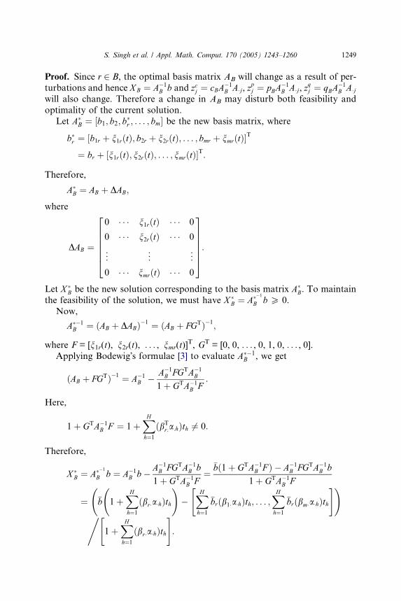
Proof. Since r 2 B, the optimal basis matrix AB will change as a result of per-
turbations and hence XB ¼ A1B b and zcj ¼ cBA
1B A�j, z
pj ¼ pBA
1B A�j, z
qj ¼ qBA
1B A�j
will also change. Therefore a change in AB may disturb both feasibility and
optimality of the current solution.
Let A�B ¼ ½b1; b2; b�r ; . . . ; bm� be the new basis matrix, where
b�r ¼ ½b1r þ n1rðtÞ; b2r þ n2rðtÞ; . . . ; bmr þ nmrðtÞ�T
¼ br þ ½n1rðtÞ; n2rðtÞ; . . . ; nmrðtÞ�T:
Therefore,
A�B ¼ AB þ DAB;
where
DAB ¼
0 � � � n1rðtÞ � � � 0
0 � � � n2rðtÞ � � � 0
..
. ... ..
.
0 � � � nmrðtÞ � � � 0
2666664
3777775:
Let X �B be the new solution corresponding to the basis matrix A�
B. To maintain
the feasibility of the solution, we must have X �B ¼ A�1
B b P 0.
Now,
A�1B ¼ ðAB þ DABÞ1 ¼ ðAB þ FGTÞ1;
where F = [n1r(t), n2r(t), . . . , nmr(t)]T, GT = [0, 0, . . . , 0, 1, 0, . . . , 0].
Applying Bodewig�s formulae [3] to evaluate A�1B , we get
ðAB þ FGTÞ1 ¼ A1B A1
B FGTA1B
1þ GTA1B F
:
Here,
1þ GTA1B F ¼ 1þ
XHh¼1
ðbTr:a:hÞth 6¼ 0:
Therefore,
X �B ¼ A�1
B b ¼ A1B b A1
B FGTA1B b
1þ GTA1B F
¼�bð1þ GTA1
B F Þ A1B FGTA1
B b
1þ GTA1B F
¼ �b
1þ
XHh¼1
ðbr�a�hÞth
!
XHh¼1
�brðb1�a�hÞth; . . . ;XHh¼1
�brðbm�a�hÞth
" # !
1þXHh¼1
ðbr�a�hÞth
" #,:
1250 S. Singh et al. / Appl. Math. Comput. 170 (2005) 1243–1260
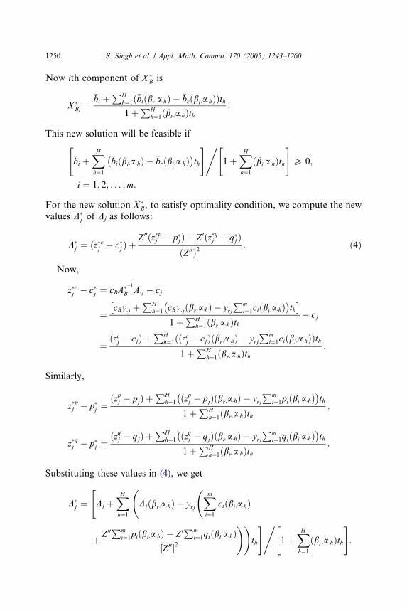
Now ith component of X �B is
X �Bi¼
�bi þPH
h¼1ð�biðbr�a�hÞ �brðbi�a�hÞÞth1þ
PHh¼1ðbr�a�hÞth
:
This new solution will be feasible if
�bi þXHh¼1
�biðbi�a�hÞ �brðbi�a�hÞ� �
th
" # "1þ
XHh¼1
ðbi�a�hÞth
#P 0
,;
i ¼ 1; 2; . . . ;m:
For the new solution X �B, to satisfy optimality condition, we compute the new
values D�j of Dj as follows:
D�j ¼ ðz�cj c�j Þ þ
Z 00ðz�pj p�j Þ Z 0ðz�qj q�j ÞðZ 00Þ2
: ð4Þ
Now,
z�cj c�j ¼ cBA�1B A�j cj
¼cBy �j þ
PHh¼1 cBy�jðbr�a�hÞ yrj
Pmi¼1ciðbi�a�hÞ
� �th
� �1þ
PHh¼1ðbr�a�hÞth
cj
¼ðzcj cjÞ þ
PHh¼1ððzcj cjÞðbr�a�hÞ yrj
Pmi¼1ciðbi�a�hÞÞth
1þPH
h¼1ðbr�a�hÞth:
Similarly,
z�pj p�j ¼ðzpj pjÞ þ
PHh¼1 ðzpj pjÞðbr�a�hÞ yrj
Pmi¼1piðbi�a�hÞ
� �th
1þPH
h¼1ðbr�a�hÞth;
z�qj p�j ¼ðzqj qjÞ þ
PHh¼1 ðzqj qjÞðbr�a�hÞ yrj
Pmi¼1qiðbi�a�hÞ
� �th
1þPH
h¼1ðbr�a�hÞth:
Substituting these values in (4), we get
D�j ¼ �Dj þ
XHh¼1
�Djðbr�a�hÞ yrjXmi¼1
ciðbi�a�hÞ "
þ Z 00Pmi¼1piðbi�a:hÞ Z 0Pm
i¼1qiðbi�a�hÞ½Z 00�2
!!th
#1þ
XHh¼1
ðbr�a�hÞth
" #,:
S. Singh et al. / Appl. Math. Comput. 170 (2005) 1243–1260 1251
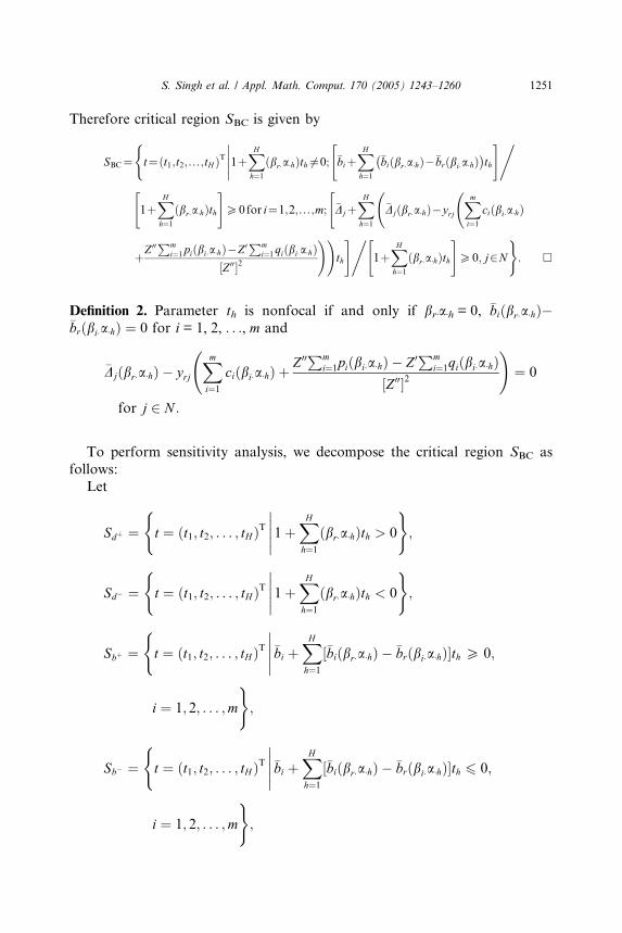
Therefore critical region SBC is given by
SBC¼ t¼ðt1;t2;...;tH ÞT 1þXHh¼1
ðbr�a�hÞth 6¼0; �biþXHh¼1
�biðbr�a�hÞ�brðbi�a�hÞ� �
th
" #,�����(
1þXHh¼1
ðbr�a�hÞth
" #P0 for i¼1;2;...;m; �Djþ
XHh¼1
�Djðbr�a�hÞyrjXmi¼1
ciðbi�a�hÞ "
þZ 00Pmi¼1piðbi�a�hÞZ 0Pm
i¼1qiðbi�a�hÞ½Z 00�2
!!th
#1þXHh¼1
ðbr�a�hÞth
" #P0; j2N
, ): �
Definition 2. Parameter th is nonfocal if and only if brÆaÆh = 0, �biðbr�a�hÞ�brðbi�a�hÞ ¼ 0 for i = 1, 2, . . ., m and
�Djðbr�a�hÞ yrjXmi¼1
ciðbi�a�hÞ þZ 00Pm
i¼1piðbi�a�hÞ Z 0Pmi¼1qiðbi�a�hÞ
½Z 00�2
!¼ 0
for j 2 N :
To perform sensitivity analysis, we decompose the critical region SBC as
follows:
Let
Sdþ ¼ t ¼ ðt1; t2; . . . ; tH ÞT 1þXHh¼1
ðbr�a�hÞth > 0
�����( )
;
Sd ¼ t ¼ ðt1; t2; . . . ; tH ÞT 1þXHh¼1
ðbr�a�hÞth < 0
�����( )
;
Sbþ ¼ t ¼ ðt1; t2; . . . ; tH ÞT �bi þXHh¼1
½�biðbr�a�hÞ �brðbi�a�hÞ�th P 0;
�����(
i ¼ 1; 2; . . . ;m
);
Sb ¼ t ¼ ðt1; t2; . . . ; tH ÞT �bi þXHh¼1
½�biðbr�a�hÞ �brðbi�a�hÞ�th 6 0;
�����(
i ¼ 1; 2; . . . ;m
);
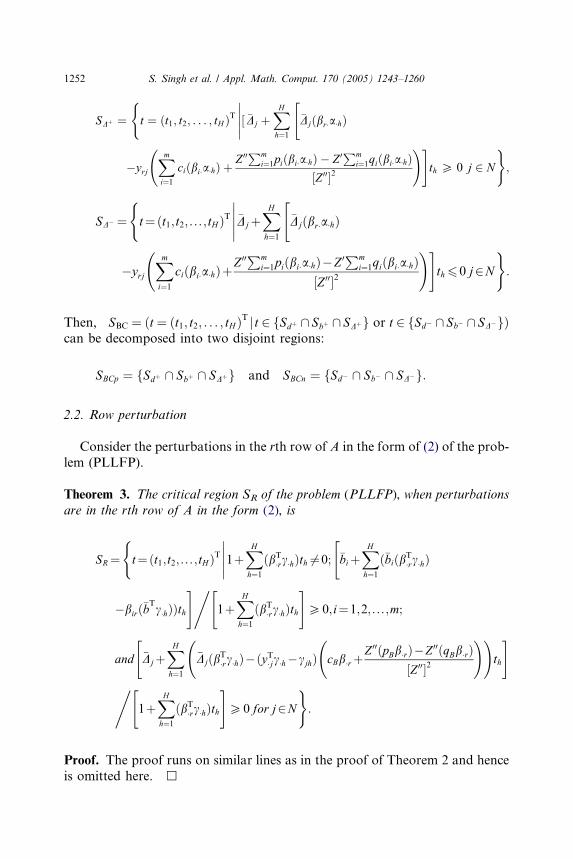
1252 S. Singh et al. / Appl. Math. Comput. 170 (2005) 1243–1260
SDþ ¼ t ¼ ðt1; t2; . . . ; tH ÞT�����½ �Dj þ
XHh¼1
"�Djðbr�a�hÞ
(
yrjXmi¼1
ciðbi�a�hÞ þZ 00Pm
i¼1piðbi�a�hÞ Z 0Pmi¼1qiðbi�a�hÞ
½Z 00�2
!#th P 0 j 2 N
);
SD ¼(t¼ðt1;t2; . .. ; tH ÞT �Djþ
XHh¼1
�Djðbr�a�hÞ"�����
yrjXmi¼1
ciðbi�a�hÞþZ 00Pm
i¼1piðbi�a�hÞZ 0Pmi¼1qiðbi�a�hÞ
½Z 00�2
!#th60 j2N
):
Then, SBC ¼ ðt ¼ ðt1; t2; . . . ; tHÞT j t 2 fSdþ \ Sbþ \ SDþg or t 2 fSd \ Sb \ SDgÞcan be decomposed into two disjoint regions:
SBCp ¼ fSdþ \ Sbþ \ SDþg and SBCn ¼ fSd \ Sb \ SDg:
2.2. Row perturbation
Consider the perturbations in the rth row of A in the form of (2) of the prob-
lem (PLLFP).
Theorem 3. The critical region SR of the problem (PLLFP), when perturbations
are in the rth row of A in the form (2), is
SR¼ t¼ðt1;t2; .. . ; tH ÞT 1þXHh¼1
ðbT�rc�hÞth 6¼0; �biþXHh¼1
ð�biðbT�rc�hÞ"�����
(
birð�bTc�hÞÞth
#1þXHh¼1
ðbT�rc�hÞth
" #P0; i¼1;2; . .. ;m;
,
and �DjþXHh¼1
�DjðbT�rc�hÞðyT�jc�hcjhÞ cBb�rþZ 00ðpBb�rÞZ 00ðqBb�rÞ
½Z 00�2
! !th
" #
1þXHh¼1
ðbT�rc�hÞth
" #P0 for j2N
, ):
Proof. The proof runs on similar lines as in the proof of Theorem 2 and hence
is omitted here. h
S. Singh et al. / Appl. Math. Comput. 170 (2005) 1243–1260 1253
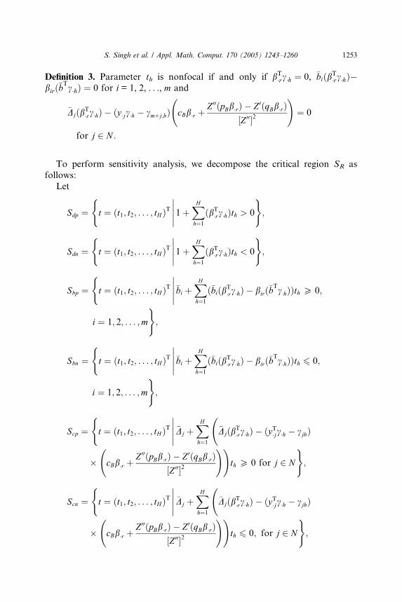
Definition 3. Parameter th is nonfocal if and only if bT�rc�h ¼ 0, �biðbT�rc�hÞbirð�b
Tc�hÞ ¼ 0 for i = 1, 2, . . ., m and
�DjðbT�rc�hÞ ðy �jc�h cmþj;hÞ cBb�r þZ 00ðpBb�rÞ Z 0ðqBb�rÞ
½Z 00�2
!¼ 0
for j 2 N :
To perform sensitivity analysis, we decompose the critical region SR as
follows:
Let
Sdp ¼ t ¼ ðt1; t2; . . . ; tH ÞT 1þXHh¼1
ðbT�rc�hÞth > 0
�����( )
;
Sdn ¼ t ¼ ðt1; t2; . . . ; tH ÞT 1þXHh¼1
ðbT�rc�hÞth < 0
�����( )
;
Sbp ¼ t ¼ ðt1; t2; . . . ; tH ÞT �bi þXHh¼1
ð�biðbT�rc�hÞ birð�bTc�hÞÞth P 0;
�����(
i ¼ 1; 2; . . . ;m
);
Sbn ¼ t ¼ ðt1; t2; . . . ; tHÞT �bi þXHh¼1
ð�biðbT�rc�hÞ birð�bTc�hÞÞth 6 0;
�����(
i ¼ 1; 2; . . . ;m
);
Scp ¼ t ¼ ðt1; t2; . . . ; tH ÞT �Dj þXHh¼1
�DjðbT�rc�hÞ ðyT�jc�h cjhÞ �����
(
� cBb�r þZ 00ðpBb�rÞ Z 0ðqBb�rÞ
½Z 00�2
!!th P 0 for j 2 N
);
Scn ¼ t ¼ ðt1; t2; . . . ; tHÞT �Dj þXHh¼1
�DjðbT�rc�hÞ ðyT�jc�h cjhÞ �����
(
� cBb�r þZ 00ðpBb�rÞ Z 0ðqBb�rÞ
½Z 00�2
!!th 6 0; for j 2 N
);
1254 S. Singh et al. / Appl. Math. Comput. 170 (2005) 1243–1260
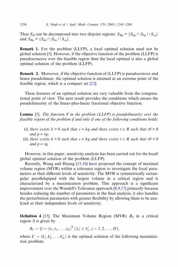
Thus SR can be decomposed into two disjoint regions: SRp = {Sdp \ Sbp \ Scp}and SRn = {Sdn \ Sbn \ Scn}.
Remark 1. For the problem (LLFP), a local optimal solution need not be
global solution [5]. However, if the objective function of the problem (LLFP) is
pseudoconcave over the feasible region then the local optimal is also a globaloptimal solution of the problem (LLFP).
Remark 2. Moreover, if the objective function of (LLFP) is pseudoconvex and
hence pseudolinear, the optimal solution is attained at an extreme point of the
feasible region, which is a compact set [12].
These features of an optimal solution are very valuable from the computa-
tional point of view. The next result provides the conditions which ensure thepseudolinearity of the linear-plus-linear fractional objective function.
Lemma [1]. The function F in the problem (LLFP) is pseudolinearity over the
feasible region of the problem if and only if one of the following conditions holds:
(i) there exists k > 0 such that c = kq and there exists t 2 R such that th > 0
and p = tq;
(ii) there exists k < 0 such that c = kq and there exists t 2 R such that th < 0and p = tq.
However, in this paper, sensitivity analysis has been carried out for the local/
global optimal solution of the problem (LLFP).
Recently, Wang and Huang [15,16] have proposed the concept of maximal
volume region (MVR) within a tolerance region to investigate the focal para-meters at their different levels of sensitivity. The MVR is symmetrically rectan-
gular parallelepiped with the largest volume in a critical region and is
characterized by a maximization problem. This approach is a significant
improvement over the Wendell�s Tolerance approach [8,9,17] primarily becausebesides reducing the number of parameters in the final analysis, it also handles
the perturbation parameters with greater flexibility by allowing them to be ana-
lyzed at their independent levels of sensitivity.
Definition 4 [15]. The Maximum Volume Region (MVR) BS in a critical
region S is given by
BS ¼ ft ¼ ðt1; t2; . . . ; tH ÞT j jtjj 6 k�j ; j ¼ 1; 2; . . . ;Hg;
where k� ¼ ðk�1; k�2; . . . ; k�H Þ is the optimal solution of the following maximiza-tion problem:
S. Singh et al. / Appl. Math. Comput. 170 (2005) 1243–1260 1255
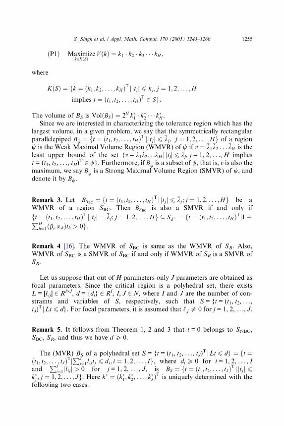
ðP1Þ Maximizek2KðSÞ
V ðkÞ ¼ k1 � k2 � k3 � � � kH ;
where
KðSÞ ¼ fk ¼ ðk1; k2; . . . ; kHÞT j jtjj 6 kj; j ¼ 1; 2; . . . ;H
implies t ¼ ðt1; t2; . . . ; tH ÞT 2 Sg:
The volume of BS is VolðBSÞ ¼ 2H k�1 � k�2 � � � k�H .Since we are interested in characterizing the tolerance region which has the
largest volume, in a given problem, we say that the symmetrically rectangular
parallelepiped Bw ¼ ft ¼ ðt1; t2; . . . ; tH ÞT j jtjj 6 �kj; j ¼ 1; 2; . . . ;Hg of a regionw is the Weak Maximal Volume Region (WMVR) of w if �v ¼ �k1�k2 . . . �kH is theleast upper bound of the set {v = k1k2. . .kH j jtjj 6 kj, j = 1, 2, . . ., H impliest = (t1, t2, . . ., tH)
T 2 w}. Furthermore, if Bw is a subset of w, that is, �v is also themaximum, we say Bw is a Strong Maximal Volume Region (SMVR) of w, anddenote it by B�w.
Remark 3. Let BSBC ¼ ft ¼ ðt1; t2; . . . ; tH ÞT j jtjj 6 �kj; j ¼ 1; 2; . . . ;Hg be a
WMVR of a region SBC. Then BSBC is also a SMVR if and only if
ft ¼ ðt1; t2; . . . ; tH ÞT j jtjj ¼ �kj; j ¼ 1; 2; . . . ;Hg � Sdþ ¼ ft ¼ ðt1; t2; . . . ; tH ÞTj1þPHh¼1ðbr�a�hÞth > 0g.
Remark 4 [16]. The WMVR of SBC is same as the WMVR of SR. Also,
WMVR of SBC is a SMVR of SBC if and only if WMVR of SR is a SMVR of
SR.
Let us suppose that out of H parameters only J parameters are obtained as
focal parameters. Since the critical region is a polyhedral set, there exists
L = [‘ij] 2 RI·J, d = {di} 2 RI, I, J 2 N, where I and J are the number of con-straints and variables of S, respectively, such that S = {t = (t1, t2, . . .,tJ)
T jLt 6 d}. For focal parameters, it is assumed that ‘.j5 0 for j = 1, 2, . . ., J.
Remark 5. It follows from Theorem 1, 2 and 3 that t = 0 belongs to SNBC,
SBC, SR, and thus we have d P 0.
The (MVR) BS of a polyhedral set S = {t = (t1, t2, . . ., tJ)T jLt 6 d} ¼ ft ¼
ðt1; t2; . . . ; tJÞTjPJ
j¼1lijtj 6 di; i ¼ 1; 2; . . . ; Ig, where di P 0 for i = 1, 2, . . . , Iand
PIi¼1jlijj > 0 for j = 1, 2, . . . , J, is BS ¼ ft ¼ ðt1; t2; . . . ; tJ ÞT j jtjj 6
k�j ; j ¼ 1; 2; . . . ; Jg. Here k� ¼ ðk�1; k�2; . . . ; k�J ÞTis uniquely determined with the
following two cases:
1256 S. Singh et al. / Appl. Math. Comput. 170 (2005) 1243–1260
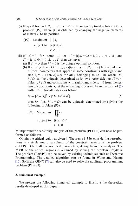
(i) If di > 0 for i = 1, 2, . . . , I, then k* is the unique optimal solution of theproblem (P2), where jLj is obtained by changing the negative elementsof matrix L to be positive
ðP2Þ MaximumY
kj
subject to jLjk 6 d;
k P 0:
(ii) If di = 0 for some i, let I� = {i jdi = 0,i = 1, 2, . . ., I}5 / and
I+ = {i jdi>0,i = 1, 2, . . ., I} then we have:(a) If I+ = / then k* = 0 is the unique optimal solution;
(b) If I+ 5 / then let X ¼S
i2I�fjjlij 6¼ 0; j ¼ 1; 2; . . . ; Jg be the index setof focal parameters that appear in some constraints with right-hand
side di = 0. Then k�j ¼ 0 for all j belonging to X. The others, k�j ,j 62 X, can be uniquely determined as follows: After deleting all vari-ables tj, j 2 X and constraints with right-hand side di = 0 from the sys-
tem of constraints S, let the remaining subsystem be in the form of (5)
with d 0i > 0 for all index i as below:
S0 ¼ ft0 ¼ ½tj�T; j 62 X jL0t0 6 d 0g ð5Þthen k*
0 (i.e., k�j ; j 62 X) can be uniquely determined by solving thefollowing problem (P3):
ðP3Þ MaximumYj 62X
kj
subject to jL0jk0 6 d 0;
k0 P 0:
Multiparametric sensitivity analysis of the problem (PLLFP) can now be per-
formed as follows:
Obtain the critical region as given in Theorems 1–3 by considering perturba-
tions in a single row or a column of the constraint matrix in the problem
(LLFP). Delete all the nonfocal parameters, if any from the analysis. The
MVR of the critical regions is obtained by solving the problem (P2)/(P3).The problem (P2)/(P3) can be solved by existing techniques such as Dynamic
Programming. The detailed algorithm can be found in Wang and Huang
[16]. Software GINO [7] can also be used to solve the nonlinear programming
problem (P2)/(P3).
3. Numerical example
We present the following numerical example to illustrate the theoretical
results developed in this paper.
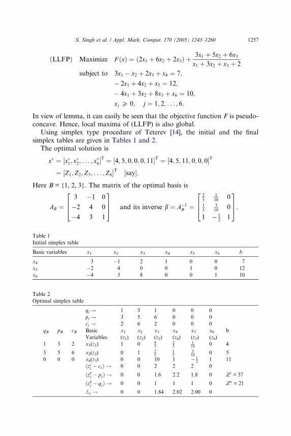
S. Singh et al. / Appl. Math. Comput. 170 (2005) 1243–1260 1257
ðLLFPÞ Maximize F ðxÞ ¼ ð2x1 þ 6x2 þ 2x3Þ þ3x1 þ 5x2 þ 6x3x1 þ 3x2 þ x3 þ 2
subject to 3x1 x2 þ 2x3 þ x4 ¼ 7;
2x1 þ 4x2 þ x5 ¼ 12;
4x1 þ 3x2 þ 8x3 þ x6 ¼ 10;
xj P 0; j ¼ 1; 2; . . . ; 6:
In view of lemma, it can easily be seen that the objective function F is pseudo-
concave. Hence, local maxima of (LLFP) is also global.
Using simplex type procedure of Teterev [14], the initial and the final
simplex tables are given in Tables 1 and 2.
The optimal solution is
x� ¼ ½x�1; x�2; . . . ; x�6�T ¼ ½4; 5; 0; 0; 0; 11�T ¼ ½4; 5; 11; 0; 0; 0�T
¼ ½Z1; Z2; Z3; . . . ; Z6�T ½say�:
Here B = {1, 2, 3}. The matrix of the optimal basis is
AB ¼3 1 0
2 4 0
4 3 1
264
375 and its inverse b ¼ A1
B ¼
25
110
015
310
0
1 121
264
375:
Table 1
Initial simplex table
Basic variables x1 x2 x3 x4 x5 x6 b
x4 3 1 2 1 0 0 7
x5 2 4 0 0 1 0 12
x6 4 3 8 0 0 1 10
Table 2
Optimal simplex table
qj! 1 3 1 0 0 0
pj! 3 5 6 0 0 0
cj! 2 6 2 0 0 0
qB pB cB Basic x1 x2 x3 x4 x5 x6 b
Variables (z1) (z2) (z3) (z4) (z5) (z6)
1 3 2 x1(z1) 1 0 45
25
110
0 4
3 5 6 x2(z2) 0 1 25
15
310
0 5
0 0 0 x6(z3) 0 0 10 1 12
1 11
ðzcj cjÞ ! 0 0 2 2 2 0
ðzpj pjÞ ! 0 0 1.6 2.2 1.8 0 Z 0 = 37
ðzqj qjÞ ! 0 0 1 1 1 0 Z00 = 21
�Mj ! 0 0 1.84 2.02 2.00 0
1258 S. Singh et al. / Appl. Math. Comput. 170 (2005) 1243–1260
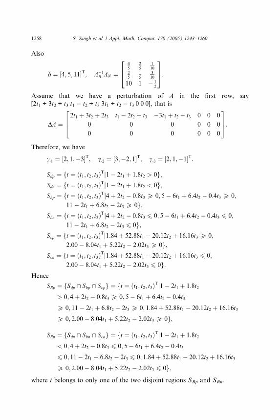
Also
�b ¼ ½4; 5; 11�T; A1B AN ¼
45
25
110
25
15
310
10 1 12
264
375:
Assume that we have a perturbation of A in the first row, say
[2t1 + 3t2 + t3 t1 t2 + t3 3t1 + t2 t3 0 0 0], that is
DA ¼2t1 þ 3t2 þ 2t3 t1 2t2 þ t3 3t1 þ t2 t3 0 0 0
0 0 0 0 0 0
0 0 0 0 0 0
264
375:
Therefore, we have
c�1 ¼ ½2; 1;3�T; c�2 ¼ ½3;2; 1�T; c�3 ¼ ½2; 1;1�T:
Sdp ¼ ft ¼ ðt1; t2; t3ÞTj1 2t1 þ 1:8t2 > 0g;Sdn ¼ ft ¼ ðt1; t2; t3ÞTj1 2t1 þ 1:8t2 < 0g;Sbp ¼ ft ¼ ðt1; t2; t3ÞTj4þ 2t2 0:8t3 P 0; 5 6t1 þ 6:4t2 0:4t3 P 0;
11 2t1 þ 6:8t2 2t3 P 0g;Sbn ¼ ft ¼ ðt1; t2; t3ÞTj4þ 2t2 0:8t3 6 0; 5 6t1 þ 6:4t2 0:4t3 6 0;
11 2t1 þ 6:8t2 2t3 6 0g;Scp ¼ ft ¼ ðt1; t2; t3ÞTj1:84þ 52:88t1 20:12t2 þ 16:16t3 P 0;
2:00 8:04t1 þ 5:22t2 2:02t3 P 0g;Scn ¼ ft ¼ ðt1; t2; t3ÞTj1:84þ 52:88t1 20:12t2 þ 16:16t3 6 0;
2:00 8:04t1 þ 5:22t2 2:02t3 6 0g:Hence
SRp ¼ fSdp \ Sbp \ Scpg ¼ ft ¼ ðt1; t2; t3ÞTj1 2t1 þ 1:8t2
> 0; 4þ 2t2 0:8t3 P 0; 5 6t1 þ 6:4t2 0:4t3
P 0; 11 2t1 þ 6:8t2 2t3 P 0; 1:84þ 52:88t1 20:12t2 þ 16:16t3
P 0; 2:00 8:04t1 þ 5:22t2 2:02t3 P 0g;
SRn ¼ fSdn \ Sbn \ Scng ¼ ft ¼ ðt1; t2; t3ÞTj1 2t1 þ 1:8t2
< 0; 4þ 2t2 0:8t3 6 0; 5 6t1 þ 6:4t2 0:4t3
6 0; 11 2t1 þ 6:8t2 2t3 6 0; 1:84þ 52:88t1 20:12t2 þ 16:16t3
P 0; 2:00 8:04t1 þ 5:22t2 2:02t3 6 0g;
where t belongs to only one of the two disjoint regions SRp and SRn.
S. Singh et al. / Appl. Math. Comput. 170 (2005) 1243–1260 1259
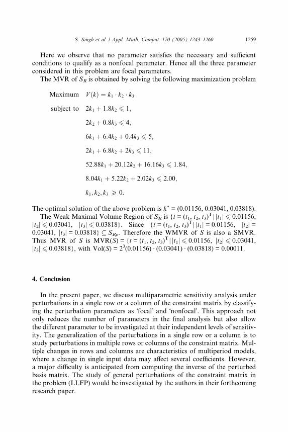
Here we observe that no parameter satisfies the necessary and sufficient
conditions to qualify as a nonfocal parameter. Hence all the three parameter
considered in this problem are focal parameters.
The MVR of SR is obtained by solving the following maximization problem
Maximum V ðkÞ ¼ k1 � k2 � k3
subject to 2k1 þ 1:8k2 6 1;
2k2 þ 0:8k3 6 4;
6k1 þ 6:4k2 þ 0:4k3 6 5;
2k1 þ 6:8k2 þ 2k3 6 11;
52:88k1 þ 20:12k2 þ 16:16k3 6 1:84;
8:04k1 þ 5:22k2 þ 2:02k3 6 2:00;
k1; k2; k3 P 0:
The optimal solution of the above problem is k* = (0.01156, 0.03041, 0.03818).
The Weak Maximal Volume Region of SR is {t = (t1, t2, t3)T j jt1j 6 0.01156,
jt2j 6 0.03041, jt3j 6 0.03818}. Since {t = (t1, t2, t3)T j jt1j = 0.01156, jt2j =
0.03041, jt3j = 0.03818} � SRp. Therefore the WMVR of S is also a SMVR.
Thus MVR of S is MVR(S) = {t = (t1, t2, t3)T j jt1j 6 0.01156, jt2j 6 0.03041,
jt3j 6 0.03818}, with Vol(S) = 23(0.01156) Æ (0.03041) Æ (0.03818) = 0.00011.
4. Conclusion
In the present paper, we discuss multiparametric sensitivity analysis underperturbations in a single row or a column of the constraint matrix by classify-
ing the perturbation parameters as �focal� and �nonfocal�. This approach notonly reduces the number of parameters in the final analysis but also allow
the different parameter to be investigated at their independent levels of sensitiv-
ity. The generalization of the perturbations in a single row or a column is to
study perturbations in multiple rows or columns of the constraint matrix. Mul-
tiple changes in rows and columns are characteristics of multiperiod models,
where a change in single input data may affect several coefficients. However,a major difficulty is anticipated from computing the inverse of the perturbed
basis matrix. The study of general perturbations of the constraint matrix in
the problem (LLFP) would be investigated by the authors in their forthcoming
research paper.
1260 S. Singh et al. / Appl. Math. Comput. 170 (2005) 1243–1260
Acknowledgements
The authors are thankful to the editor and esteemed referees for their eval-
uation of the paper. The authors also wish to express their deep gratitude
Professor R.N. Kaul, Department of Mathematics, University of Delhi, Delhi
and Professor M.C. Puri, Department of Mathematics, I.I.T., Delhi for theirencouragement and inspiration to complete the work.
References
[1] A. Cambini, L. Martein, S. Schaible, On the pseudoconvexity of the sum of two linear
fractional functions, Proceedings of the 7th International Symposium on Generalized
Convexity/Monotonicity, Aug. 27–31, 2002, Hanoi, Vietnam, to appear in Nonconvex
Optimization and its Applications, 77, 2005.
[2] S.S. Chadha, Dual of the sum of a linear and linear fractional program, European Journal of
Operational Research 67 (1993) 136–139.
[3] T. Gal, H.J. Greenberg, Advances in Sensitivity Analysis and Parametric Programming,
Kluwer Academic Press, Boston, MA, 1997.
[4] J. Hirche, On programming problems with a linear-plus-linear fractional objective function,
Cahiers du Centre d�Etudes de Recherche Operationelle 26 (1–2) (1984) 59–64.[5] J. Hirche, A note on programming problems with linear-plus-linear fractional objective
functions, European Journal of Operational Research 89 (1996) 212–214.
[6] H.C. Joksch, Programming with fractional linear objective functions, Naval Research
Logistics Quarterly 11 (1964) 197–204.
[7] J. Liebman, L. Ladson, L. Scharge, A. Waren, Modeling and Optimization with GINO, The
Scientific Press, San Francisco, CA, 1986.
[8] N. Ravi, R.E. Wendell, The tolerance approach to sensitivity analysis of matrix coefficients in
linear programming, Management Science 35 (1989) 1106–1119.
[9] N. Ravi, R.E. Wendell, The tolerance approach to sensitivity analysis of matrix coefficients in
linear programming: general perturbations, Journal of Operational Research Society 36 (10)
(1985) 943–950.
[10] S. Schaible, A note on the sum of a linear and linear fractional functions, Naval Research
Logistics Quarterly 24 (1977) 691–693.
[11] S. Schaible, Fractional programming: Applications and algorithms, European Journal of
Operational Research 7 (1981) 111–120.
[12] S. Schaible, Simultaneous optimization of absolute and relative terms, Z. Angew. Math. Mech.
64 (8) (1984) 363–364.
[13] S. Singh, P. Gupta, D. Bhatia, Multiparametric sensitivity analysis in programming problems
with linear-plus-linear fractional objective function, European Journal of Operational
Research 160 (2005) 232–241.
[14] A.G. Teterev, On a generalization of linear and piecewise linear programming, Matekon 6
(1970) 246–259.
[15] H.F. Wang, C.S. Huang, Multi-parametric analysis of the maximum tolerance in a linear
programming problem, European Journal of Operational Research 67 (1993) 75–87.
[16] H.F. Wang, C.S. Huang, The maximal tolerance analysis on the constraint matrix in linear
programming, Journal of the Chinese Institute of Engineers 15 (5) (1992) 507–517.
[17] R.E. Wendell, The tolerance approach to sensitivity analysis in linear programming,
Management Science 31 (1985) 564–578.