arX

iv:0

906.

1608

v1 [

cond

-mat

.mtr

l-sc

i] 8

Jun

200

9

Multicomponent multisublattice alloys, nonconfigurational entropy

and other additions to the Alloy Theoretic Automated Toolkit

A. van de Walle

June 8, 2009

Abstract

A number of new functionalities have been added to the Alloy Theoretic Automated Toolkit (ATAT)since it was last reviewed in this journal in 2002. ATAT can now handle multicomponent multisublatticealloy systems, nonconfigurational sources of entropy (e.g. vibrational and electronic entropy), SpecialQuasirandom Structures (SQS) generation, tensorial cluster expansion construction and includes inter-faces for multiple atomistic or ab initio codes. This paper presents an overview of these features gearedtowards the practical use of the code. The extensions to the cluster expansion formalism needed to covermulticomponent multisublattice alloys are also formally demonstrated.

1 Introduction

The Alloy Theoretic Automated Toolkit (ATAT) [1–3] is a suite of software tools facilitating the determi-nation of thermodynamic properties of solid state alloys from first-principles calculations. It relies upon thecluster expansion formalism [4–11] to build a simplified effective Hamiltonian that accurately reproducesquantum mechanical calculation results for an alloy system of interest and that can be used to efficientlycalculate their thermodynamic properties. ATAT is freely distributed and open-source, thus encouragingusers to contribute [12].

ATAT’s basic functionalities have been described in an earlier issue of the CALPHAD journal [1]. Sincethen, a number of new features have been added and the purpose of the present paper is to describe theseadditions and provide a concise “user guide” for these new features. The most significant additions to ATATare

1. extensions to multicomponent multisublattice systems;

2. the inclusion of nonconfigurational sources of entropy (vibrational and electronic entropy);

3. Special Quasirandom Structures (SQS) generation;

4. tensorial cluster expansion construction;

5. support for multiple atomistic (ab initio) codes;

6. various new conversion and analysis utilities.

The features presented here are not exhaustive and new features are continuously being added. Hence,the reader is invited to consult the manual supplied with the ATAT distribution or posted on the ATAT website ( http://alum.mit.edu/www/avdw/atat ) for the most up to date information.

2 Multicomponent multisublattice systems

2.1 The cluster expansion in multicomponent multisublattice systems

The traditional cluster expansion represents the relationship q (σ) between a configuration σ and somescalar intensive quantity q. While multicomponent alloys have been covered since the original introduction

1

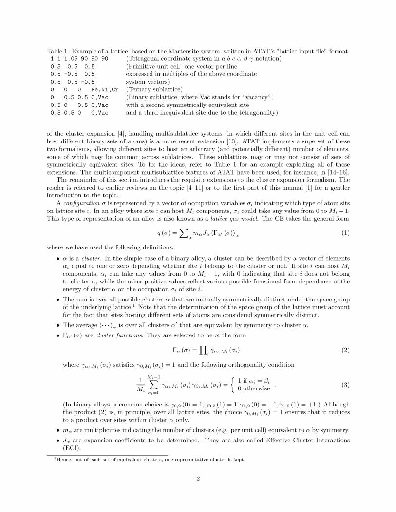
Table 1: Example of a lattice, based on the Martensite system, written in ATAT’s ”lattice input file” format.1 1 1.05 90 90 90 (Tetragonal coordinate system in a b c α β γ notation)0.5 0.5 0.5 (Primitive unit cell: one vector per line0.5 -0.5 0.5 expressed in multiples of the above coordinate0.5 0.5 -0.5 system vectors)0 0 0 Fe,Ni,Cr (Ternary sublattice)0 0.5 0.5 C,Vac (Binary sublattice, where Vac stands for “vacancy”,0.5 0 0.5 C,Vac with a second symmetrically equivalent site0.5 0.5 0 C,Vac and a third inequivalent site due to the tetragonality)

of the cluster expansion [4], handling multisublattice systems (in which different sites in the unit cell canhost different binary sets of atoms) is a more recent extension [13]. ATAT implements a superset of thesetwo formalisms, allowing different sites to host an arbitrary (and potentially different) number of elements,some of which may be common across sublattices. These sublattices may or may not consist of sets ofsymmetrically equivalent sites. To fix the ideas, refer to Table 1 for an example exploiting all of theseextensions. The multicomponent multisublattice features of ATAT have been used, for instance, in [14–16].

The remainder of this section introduces the requisite extensions to the cluster expansion formalism. Thereader is referred to earlier reviews on the topic [4–11] or to the first part of this manual [1] for a gentlerintroduction to the topic.

A configuration σ is represented by a vector of occupation variables σi indicating which type of atom sitson lattice site i. In an alloy where site i can host Mi components, σi could take any value from 0 to Mi − 1.This type of representation of an alloy is also known as a lattice gas model. The CE takes the general form

q (σ) =∑

αmαJα 〈Γα′ (σ)〉α (1)

where we have used the following definitions:

• α is a cluster. In the simple case of a binary alloy, a cluster can be described by a vector of elementsαi equal to one or zero depending whether site i belongs to the cluster or not. If site i can host Mi

components, αi can take any values from 0 to Mi − 1, with 0 indicating that site i does not belongto cluster α, while the other positive values reflect various possible functional form dependence of theenergy of cluster α on the occupation σi of site i.

• The sum is over all possible clusters α that are mutually symmetrically distinct under the space groupof the underlying lattice.1 Note that the determination of the space group of the lattice must accountfor the fact that sites hosting different sets of atoms are considered symmetrically distinct.

• The average 〈· · · 〉α is over all clusters α′ that are equivalent by symmetry to cluster α.

• Γα′ (σ) are cluster functions. They are selected to be of the form

Γα (σ) =∏

iγαi,Mi

(σi) (2)

where γαi,Mi(σi) satisfies γ0,Mi

(σi) = 1 and the following orthogonality condition

1

Mi

Mi−1∑

σi=0

γαi,Mi(σi) γβi,Mi

(σi) =

{

1 if αi = βi

0 otherwise. (3)

(In binary alloys, a common choice is γ0,2 (0) = 1, γ0,2 (1) = 1, γ1,2 (0) = −1, γ1,2 (1) = +1.) Althoughthe product (2) is, in principle, over all lattice sites, the choice γ0,Mi

(σi) = 1 ensures that it reducesto a product over sites within cluster α only.

• mα are multiplicities indicating the number of clusters (e.g. per unit cell) equivalent to α by symmetry.

• Jα are expansion coefficients to be determined. They are also called Effective Cluster Interactions(ECI).

1Hence, out of each set of equivalent clusters, one representative cluster is kept.

2

It can be shown that when all clusters α are considered in the sum, the cluster expansion is able torepresent any function q (σ) of configuration σ by an appropriate selection of the values of Jα. The cruxof the argument leading to that conclusion lies in establishing that the Γα (σ) form an orthogonal basis forthe space of functions of configurations according to a suitably defined inner product. In the general caseconsidered here, the original proof [4] needs to be extended as follows. Given two cluster functions Γα andΓβ associated with two corresponding clusters α and β, define the inner product:

〈Γα, Γβ〉 =∑

σ

Γα (σ) Γβ (σ)

where the sum is over all possible configurations σ (i.e., each σi ranges from 0 to Mi − 1 in lexicographicorder). We can then note that

〈Γα, Γβ〉 =1

∏

i Mi

∑

σ

(

∏

iγαi,Mi

(σi))(

∏

iγβi,Mi

(σi))

=1

M1

M1−1∑

σ1=0

1

M2

M2−1∑

σ2=0

. . .∏

i(γαi,Mi

(σi) γβi,Mi(σi))

=∏

i

[

1

Mi

Mi−1∑

σi=0

(γαi,Mi(σi) γβi,Mi

(σi))

]

where the term in bracket is zero for any i such that αi 6= βi by Equation (3). If no such i exist, theneach term in bracket is equal to 1. It follows that 〈Γα, Γβ〉 = 0 if the clusters α and β differ (even by asingle site) and is equal to 1 if they are identical. This establishes that the Γα are orthogonal. Moreover,there are as many different α as there are different σ (as αi and σi both can take on Mi distinct values),so the “number” of Γα equals2 the “dimension” of the configurational space σ. It follows that the Γα forma complete orthogonal basis. This result is not obvious when lattice sites may host a different number ofspecies (i.e. when Mi is not constant). In that case, the cluster functions (Equation (2)) may involve mixedproducts between entirely different types of γαi,Mi

(σi).While, the above discussion is valid for any γαi,Mi

(σi) satisfying (3), a specific γαi,Mi(σi) must be selected

in practice. By default, the ATAT uses the following choice:

γαi,Mi(σi) =

1 if αi = 0− cos(2π

⌈

αi

2

⌉

σi

M) if αi > 0 and odd

− sin(2π⌈

αi

2

⌉

σi

M) if αi > 0 and even

where ⌈. . .⌉ denotes the “round up” operation and where both αi and σi can range from 0 to Mi − 1. Notethat these functions reduce to the single function − (−1)

σi in the binary case (Mi = 2). User-specifiedγαi,Mi

(σi) can be provided by (i) editing and following the instructions given in the corrskel.c++ file andby (ii) specifying the -crf=[keyword] option on the command line of ATAT commands, where [keyword]

is a unique identifier.Another nonobvious aspect of the above cluster expansion generalization is that the relationship between

the point correlations and the composition variables is no longer as trivial as in the well-known singlesublattice binary case. In general, there are three different composition-type quantities to consider, eachhaving a specific use.

1. The point correlation vector ρ contains all the expected values of the cluster functions 〈Γα (σ)〉 asso-ciated with a cluster α such that αi is nonzero for a single site i. They enter the expression of thecluster expansion which is used to predict energies either during the ground state search procedure orin the Monte Carlo simulations.

2. The “nonredundant” concentration vector c are those that remain after all linearly dependent con-centrations have been eliminated (of course, there are multiple valid choices of nonredundant concen-trations — one convention must be arbitrarily selected). These linear dependencies arise from the

2This statement can be made more rigorous by considering a sequence of finite system (with periodic boundary conditions)whose size increases to infinity.

3

constraint that the compositions on each sublattice sum up to one. The nonredundant concentrationsare used for the convex hull construction in the ground state search procedure.

3. The full vector x of concentrations has no algorithmic use but provides the most user-friendly output.

These quantities are linearly related:

c = Cρ + c0 (4)

x = Xρ + x0 (5)

where C and X are constant matrices while c0 and x0 are constant vectors. In general, the matrices C andX are rectangular and not invertible. (These matrices can be output within ATAT with the corrdump -pcm

command, if the user provides a lattice input file lat.in.) Appendix A describes how these matrices arecalculated.

The matrix X plays a special role in the conversion of chemical potentials µ into shifts of the effectivecluster interactions Jα, as would be needed in a grand canonical Monte Carlo simulation. Note that thechemical potential contribution to any of the grand canonical thermodynamic functions can be written as

µT x = µT Xρ + µT x0 =(

XT µ)T

ρ + µT x0 =∑

j

(

XT µ)

jρj + µT x0

from which it can be inferred that µT x0 is the shift induced in the empty cluster ECI, while the j-elementof the vector XT µ is the shift induced in the ECI associated with point correlation ρj.

2.2 Multicomponent cluster expansion construction

The mmaps command is the multicomponent version of the maps command (discussed in [1, 2]) and worksin a similar fashion. It gradually constructs an increasingly more accurate cluster expansion by repeatedlyinvoking a first-principles code through auxiliary scripts (see Sections 3, 6 and the documentation of thepollmach and runstruct xxxx commands for details). The main difference between the mmaps and maps

codes is that, given the larger number of components allowed in mmaps, the input and output files have tocontain more information. The main input file (typically called lat.in), which describes the lattice, is anatural extension of the maps input file, as shown in Table 1.

A second, optional, input file (typically called crange.in) provides the ability to specify a region toexplore in composition space. This is useful in systems where the provided lattice would be mechanicallyor thermodynamically unstable beyond certain composition limits. For instance, given the lattice shown inTable 1, one could specify:

1*Ni+1*Cr<=0.2

1*C<=0.1

where each atom name stands for its overall concentration (it is not the concentration on a sublattice).Only linear constraints are supported (and are implicitly combined with a logical “and”, so that the allowedregions are necessarily convex).

This file not only controls the range of concentration of the structures generated by mmaps, but also thecomposition range where the correct ground states are enforced in the fitting process. Note that, occasionally,structures outside the specified range may be generated in order to ensure that the ground states found withinthe specified composition range are not masked by ground states outside of it (mmaps internally generatesstructures at all compositions in order to check for this).

Suitable composition limits are not always known in advance. When these limits arise due to mechanicalinstabilities, one would notice that many of the structures generated by mmaps relax to very different types oflattices. A symptom of this is the inability to converge the cluster expansion. A way to check for this problemis to use the checkrelax utility, which calculates the mean square of the relaxation strain tensor elementsfor each of the structures generated by mmaps. Note that, by design, this command ignores the isotropiccomponent of the strain. It compares relaxed geometries in the */str relax.out files to the correspondingunrelaxed */str.out files. Any value above 0.1 should be regarded as suspect. While having a few isolatedoverrelaxed structures is not typically a problem, if virtually all structures beyond a certain composition

4

limit are relaxing excessively, then it is advisable to specify a suitable crange.in file and restart mmaps. Itis also recommended to “hide” any overrelaxed structures by issuing the command

touch [structure]/error

for each [structure] exhibiting overrelaxation (typically [structure] is a number referring to one of thesubdirectories generated by mmaps and containing a structure’s geometry). This command creates files callederror in the specified directory that mmaps will perceive as a signal to ignore the structure in question.

The relevant composition region is sometimes limited by thermodynamic instabilities. This would bedetected, for instance, by doing a separate cluster expansion on a different lattice or by computing theformation energies of known compounds exhibiting a different lattice. In such cases, however, it is notessential to limit the compositions range, since the cluster expansion formalism remains valid for metastablealloys. However, unless the metastable region is of direct interest, a more rapidly converging cluster expansionmay be obtained by specifying a suitable crange.in file and by excluding non-ground state structures inthe metastable region with the touch command, as explained above.

It is sometimes tempting to perform a cluster expansion under equality — rather than inequality —composition constraints. This is relevant for ionic systems, where it may be most natural to only keepstructures that are “charge balanced” under the assumption that all species keep their nominal charges.This is not implemented in mmaps, because it is very risky approach. A cluster expansion providing anexcellent fit to charge-balanced structures may inadvertently predict non-charge-balanced ground states. Away to prevent such problems [13] is to restrict compositions to lie in a nonzero-width slice around thecharge-balanced hyperplane, as in the following example for the Samarium-doped Ceria system [14]:

-2*O+4*Ce+3*Sm<=0.2

-2*O+4*Ce+3*Sm>=-0.2

mmaps will, if necessary, sample structures outside of the specified range to ensure that no spurious non-charge-balanced ground states exist.

Compared to maps, the mmaps code has a number of new output files. The atoms.out file lists all atomicspecies given in the input files in the order that will be used to report composition variables in all output

files. The ref energy.out file reports the atomic reference energies used to calculate formation energies inall output files (in the same order as in atoms.out). These reference energies are the energies of the pureelements, if they are included in the fit. Otherwise, if composition constraints are imposed,3 the structureswith the most extreme compositions4 are used as reference. These non-standard references are convertedinto atomic energies before being output in ref energy.out. This default behavior can be overridden byproviding user-specified reference energies in a file called ref energy.in.

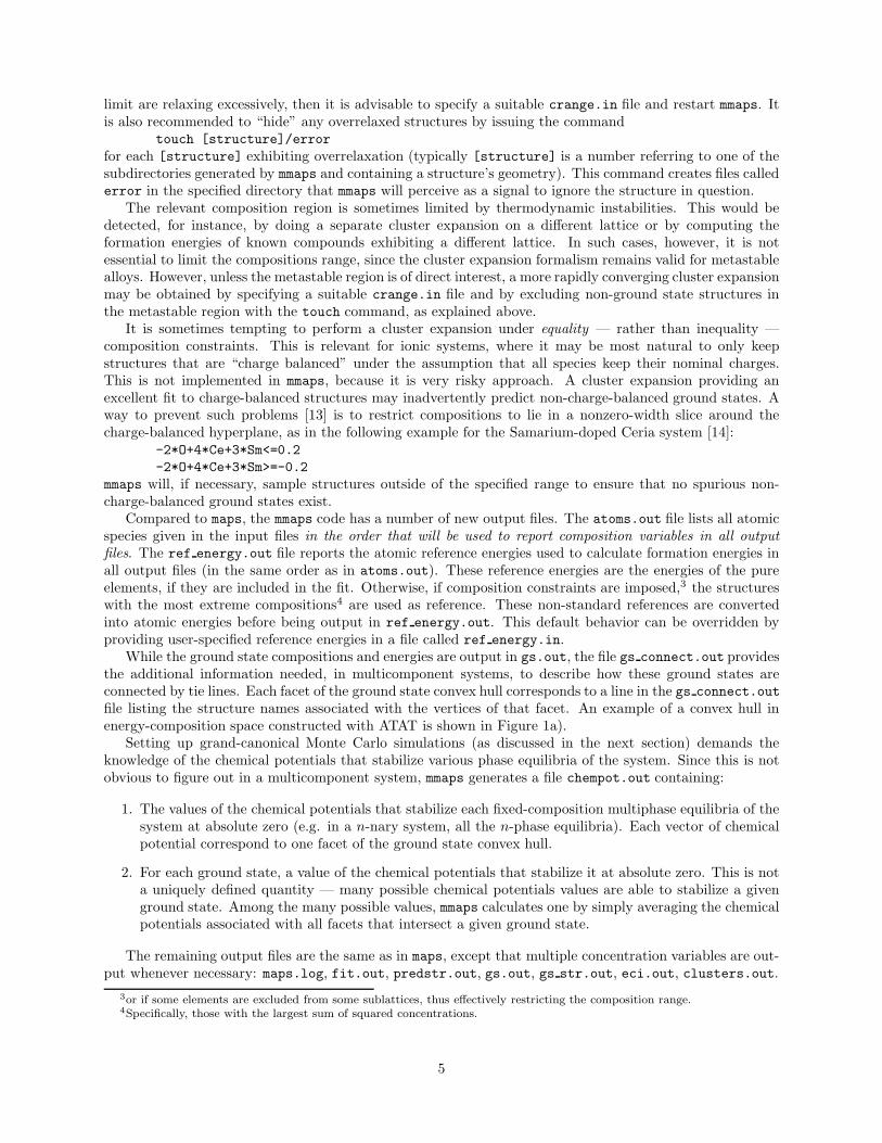
While the ground state compositions and energies are output in gs.out, the file gs connect.out providesthe additional information needed, in multicomponent systems, to describe how these ground states areconnected by tie lines. Each facet of the ground state convex hull corresponds to a line in the gs connect.out

file listing the structure names associated with the vertices of that facet. An example of a convex hull inenergy-composition space constructed with ATAT is shown in Figure 1a).

Setting up grand-canonical Monte Carlo simulations (as discussed in the next section) demands theknowledge of the chemical potentials that stabilize various phase equilibria of the system. Since this is notobvious to figure out in a multicomponent system, mmaps generates a file chempot.out containing:

1. The values of the chemical potentials that stabilize each fixed-composition multiphase equilibria of thesystem at absolute zero (e.g. in a n-nary system, all the n-phase equilibria). Each vector of chemicalpotential correspond to one facet of the ground state convex hull.

2. For each ground state, a value of the chemical potentials that stabilize it at absolute zero. This is nota uniquely defined quantity — many possible chemical potentials values are able to stabilize a givenground state. Among the many possible values, mmaps calculates one by simply averaging the chemicalpotentials associated with all facets that intersect a given ground state.

The remaining output files are the same as in maps, except that multiple concentration variables are out-put whenever necessary: maps.log, fit.out, predstr.out, gs.out, gs str.out, eci.out, clusters.out.

3or if some elements are excluded from some sublattices, thus effectively restricting the composition range.4Specifically, those with the largest sum of squared concentrations.

5

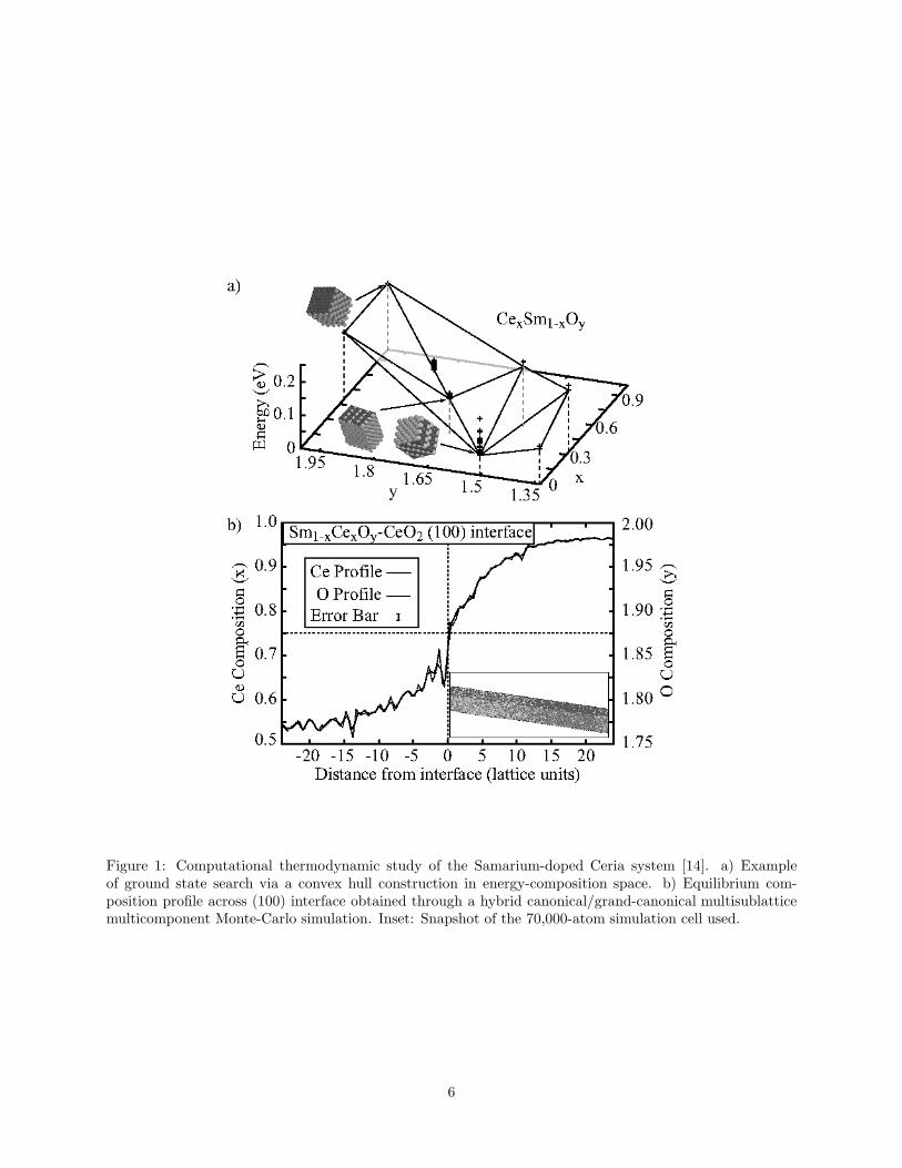
Figure 1: Computational thermodynamic study of the Samarium-doped Ceria system [14]. a) Exampleof ground state search via a convex hull construction in energy-composition space. b) Equilibrium com-position profile across (100) interface obtained through a hybrid canonical/grand-canonical multisublatticemulticomponent Monte-Carlo simulation. Inset: Snapshot of the 70,000-atom simulation cell used.

6

Table 2: Example of control.in file indicating a scan of the region in (T, µ1, µ2, µ3)-space defined by100 ≤ T < 200 and 0 ≤ µ1 < 1.0 and 0 ≤ µ2 < 0.5 and µ3 = 0.0 with a 10 × 5 × 5 grid.100 0.0 0.0 0.0

200 0.0 0.0 0.0 10

100 0.0 0.5 0.0 5

100 1.0 0.0 0.0 5

2.3 Hybrid Multicomponent Monte Carlo simulations

The memc2 code implements general hybrid canonical/grand-canonical lattice gas Monte Carlo simulations inmulticomponent systems. As most of the features are similar to the previous binary version, emc2, describedin [1, 3], we focus here on the differences.

To function, this code requires at least 4 input files: lat.in (identical to the one input into mmaps),clusters.out, eci.out, gs str.out, where the latter three are generated by mmaps. Given the largernumber of composition variables, the range of temperatures and chemical potentials scanned in the course ofgrand-canonical run are no longer specified on the command-line. Instead, the control.in input file mustbe provided in the following format. The first line specify the initial conditions and has the form (for ann-component system):

[T] [µ1] ... [µn]

where T is temperature and µ1, . . . , µn are the chemical potentials for each chemical species, in the sameorder as in the atoms.out file generated by mmaps.5 Each subsequent line of this file indicates one of theaxes along which to scan and has the format:

[T] [µ1] ... [µn] [s]where s is the the number of steps made between the initial conditions and the final conditions given on theline. Table 2 gives an example of such file.

A few important notes:

1. Temperatures are given in units of energy unless the -k or -keV options are used (the latter indicatestemperature in K if energies are in eV).

2. By default, the finals conditions are excluded from the scan (in the example above the values of thefirst chemical potential scanned (see the last line) are 0.0 0.2 0.4 0.6 0.8). This behavior can be changedwith the -il option, to give: 0.0 0.25 0.5 0.75 1.0). Alternatively, the -hf option gives: 0.1 0.3 0.5 0.70.9.

3. The mmaps code generates a file called chempot.out which contains special values of the chemicalpotential that stabilize various types of equilibria. These values are useful guidelines to select relevantregions in µ-space to scan.

Canonical or hybrid canonical/grand-canonical simulations can be carried out by specifying, in a file calledconccons.in, a set of linear constraints on the composition that must hold throughout the simulation. Thecode automatically generates a complete list of allowed multi-site Monte Carlo moves. It does so by firstconsidering all possible single-atom identity flips (k = 1), then all possible two-atom identity flips (k = 2),etc. Any move violating the composition constraints is eliminated. After all k-atom flips that satisfy theconstraints have been considered, the code calculates the linear subspace spanned by the composition changesassociated these flips. The process stops if this linear subspace has the same dimension as the space of allowedcompositions. The moves generated by this process are guaranteed to satisfy detailed balance because forevery move kept, its reverse move is also kept.

The format of the conccons.in file is similar to the crange.in file of mmaps. For instance:-2*O+4*Ce+3*Sm=0

would ensure overall charge balance in the fluorite-type CexSm1−xOyVac2−y system. Constraining com-position variables is particularly useful to pin down the location of an interface in a multiphase interfacial

5Alternatively, see the ouput of corrdump -pcm.

7

thermodynamic calculation, because the phase fractions are uniquely determined by the overall composition.An example of this use is illustrated in Figure 1b).

Any number of constraints can be given up to the point where all concentration variables are fixed, whichresults in a fully canonical simulation. Note that constant composition simulations do not evade the needto make sure that the cluster expansion does not exhibit spurious ground states away from the specifiedhyperplane. If such ground states exist, the Monte Carlo code will reveal a phase separation into regionsthat do not locally satisfy the composition constraint, although the overall simulation cell does. Note thatthe constant specified on the right-hand side of the conccons.in file is ignored — this file constrains changesin composition only. The user-supplied initial atomic configuration (via the -g=[ground state number] or-is=[file] options) implicitly determines the right-hand side constants.

The memc2 code outputs all of thermodynamic quantities it computes on the standard output and in a logfile mc.out. Given the large (and variable) number of variables in a multicomponent system, the code writesa mcheader.out file indicating the content of each column of the main output file. By default all outputquantities are grand-canonical in nature (i.e. they contain a “−µ · x” term, where x is composition and µchemical potential), regardless of the presence of composition constraints. To obtain “canonical” rather thangrand-canonical quantities use the -g2c option.

In addition to performing Monte Carlo simulations, the memc2 code reports thermodynamic quantitiescalculated via the low-temperature expansion (indicated by a lte suffix ) or the mean-field approximation6

(indicated by a mf suffix ). A useful feature is the ability to skip Monte Carlo simulations whenever the freeenergies obtained via mean-field approximation and the low temperature expansion fall within a specifiedthreshold (using the -mft=[tolerance] option), as this indicates that either one is sufficiently accurate.These approximations are also used to set initial values of the free energy when performing thermodynamicintegrations. By default, if the initial configuration is a ground state (-gs=[a positive integer]) the low-temperature expansion provides the starting point while Monte Carlo averages are used to update the freeenergy as temperature and chemical potentials are varied. If the initial configuration is the fully disorderedstate (-gs=-1) a mean-field approximation (i.e. high-temperature expansion) is used as the starting pointinstead.

Finally, it is possible to specify temperature-dependent interactions (in a file called teci.out, which,when present, takes precedence over eci.out). This feature can be used to account for nonconfigurationalsources of entropy through a coarse-graining scheme [17, 18]. Introducing temperature-dependent interactionsis not completely trivial, as various averages (such as the internal energy E) must correctly account for thetemperature dependence of the interactions in order for the following thermodynamic relationship (uponwhich thermodynamic integration is based) to hold:

∂ (βF )

∂β= E

where β = (kBT )−1 and F is the Helmholtz free energy. To illustrate this, we express the free energy F interms of the partition function and the coarse grained free energy7 Fi of each microscopic state i:

∂ (βF )

∂β= −

∂

∂βln

(

∑

i

e−βFi

)

=

∑

i [Fi + β (∂Fi/∂β)] e−βFi

∑

i e−βFi.

Hence, the quantity to average over the Monte Carlo steps is [Fi + β (∂Fi/∂β)] instead of just Fi, as a naiveanalogy with the constant interaction case would have suggested.

The next section describes how to proceed to obtain suitable temperature-dependent interactions thatmodel vibrational and electronic excitations.

6While the emc2 code also reports the high-temperature limit, this was abandoned in the memc2 code since it is identical themean-field values for the pure phases.

7In a coarse-graining framework, each microscopic configurational state i has a free energy that can be expressed in termsof a partition function summing over all vibrational and electronic excitations j associated with a given configuration i on the

lattice: Fi = −β−1 ln“

P

j e−βEj

”

.

8

3 Nonconfigurational sources of entropy

3.1 Lattice vibrations

The ATAT software offers two techniques to calculate vibrational free energies.The fitfc code constructs a Born-von Karman spring model by fitting the reaction forces resulting from

imposed atomic displacements in a supercell calculation [17, 19, 20]. This is the preferred method8 for veryaccurate calculations, since the range of interactions of the model’s effective springs can be increased untilthe desired accuracy has been reached. However, it is computationally demanding to calculate vibrationalfree energies for a large number of structures in this fashion (as would be required for cluster expansionconstruction).

For this reason, ATAT includes an alternative method: The stiffness-vs.-length scheme [17], which isimplemented in the fitsvsl and svsl codes. This approach exploits the fact that the effective springsof a Born-von Karman model are often transferable from one structure to another (after controlling forsimple factors such as bond length [17, 27–29], or composition [30]), thus reducing the number of springconstant calculations needed. This method’s accuracy is limited by the transferability assumption itself,which typically does not extend beyond nearest neighbor springs. Fortunately, this assumption is verifiableand we shall see how.

3.1.1 The fitfc code

Calculations with the fitfc code proceed in a series of steps:

1. The structure of interest first needs to be fully relaxed. The code expects the relaxed geometry in afile called str relax.out. This file’s format is common to all ATAT tools and is described in [1] aswell as in the help obtained via mmaps -h. The fitfc command also expects a str.out file containingthe unrelaxed geometry (which may be the same as the relaxed geometry, if desired). The unrelaxedgeometry will be used to determine the neighbor shells and measure distances between atoms. Therationale for allowing for two types of input structures is that it is easier for most users to specify oridentify shells of neighbor using “idealized” structures (e.g. hcp with ideal c/a ratio) rather than usingthe fully relaxed structures. Moreover, in the context of cluster expansion construction, where phononcalculations on multiple structures are needed, the neighbor shell distances are directly transferablebetween unrelaxed structures but not between relaxed structures.Typically the user would specify the str.out and then obtain the str relax.out file by running anab initio code with a command of such as runstruct xxxx, where xxxx stands for the name of the abinitio code used (see Section 6 below for calling ab initio codes within ATAT). Of course, the inputfiles for the xxxx code must indicate that all degrees of freedom need to be relaxed. Alternatively, filestr.out and str relax.out files could have been automatically generated in a prior mmaps execution(in fact, the perhaps odd extension .out reflects the fact that these files are typically outputs of themmaps and runstruct xxxx codes.).

2. Next, a set of perturbed geometries must be generated. A typical command line is as follows:fitfc -er=11.5 -ns=3 -ms=0.02 -dr=0.1

The -er option specifies how far apart the periodic images of the displaced atom must be (as measuredin the unrelaxed structure str.out and in the same units, usually A). The code uses this informationto finds the smallest supercell satisfying this constraint. While this is the only required parameter, theuser has control over other parameters.-dr specifies the magnitude of the displacement (default: 0.2 A) of the perturbed atom (in the sameunits as in the str.out file, typically A)-ns specifies the number of different isotropic strain levels at which phonon calculations will be per-formed. Specifying -ns=1 implies a purely harmonic model (the default), while values greater than 1will invoke a quasiharmonic model. The latter accounts for thermal expansion by allowing the phonon

8In principle, linear response calculations [21–26] are even more preferable in the sense that they account for infinite rangeinteractions, which is important in the case of ionic materials. Linear response calculations are to be performed within the abinitio code itself and ATAT consequently does not implement them.

9

frequencies to be volume-dependent. In subsequent steps, the code will determine the volume as afunction of temperature by minimizing the free energy.-ms specifies the maximum level of strain (e.g. 0.02 signifies a 2% elongation along every direction).The above command writes out a series of subdirectories of the general form vol *, one for each levelof strain (* refers to the usual UNIX wildcard).If the structure has cubic symmetry and no internal degrees of freedom or if one only wishes to use theharmonic approximation, the fitfc command should be invoked with the -nrr option (do Not ReRelax).In these case, the relaxation step 3 below can be skipped.

3. Each vol * subdirectory now contains a str.out file which is stretched version of the main str relax.out

file provided. (This naming convention is a bit confusing but is dictated by the fact that thesevol */str.out files are the starting point of another relaxation step.) The ab initio code then needsto be invoked to rerelax the geometry at the various levels of imposed strain and obtain the energy asa function of strain. Typically, this is achieved by typing:9

pollmach -e runstruct xxxx -w ionrelax.wrap

The pollmach -e . . . prefix causes the command specified next to be run in all subdirectories con-taining a file called wait (a file automatically written by fitfc with this purpose in mind) beforeexiting. Here, the command to be run is runstruct xxxx, which invokes the ab initio code xxxx. Theoption -w ionrelax.wrap specifies an alternative user-specified input file for the ab initio code, whichmust indicate that all degrees of freedom except volume must be allowed to relax. This additionalrelaxation step is needed because stretching may have modified the equilibrium atomic positions. Therelaxed (but stretched) structures now reside in the vol */str relax.out files while the correspondingenergies will be in vol */energy.

4. Now, one needs to invoke fitfc again to generate perturbations of the atomic position for each levelof strain, e.g.:

fitfc -er=11.5 -ns=3 -ms=0.02 -dr=0.1

This is exactly the same command as before but the code notices the presence on the new files andproceeds further.At this point the files generated are arranged as follows. At the top level, there is one subdirectory perlevel of strain (vol *, where * is the strain in percent), and in each subdirectory, there are a numberof subsubdirectories, each containing a different perturbation. The perturbation names have the form

p[+/-][dr] [er] [index],where [pertmag] is the number given by the -dr option, [er] the number given by the -er optionand [index] is a number used to distinguish between different perturbations. Two perturbations thatdiffer only by their signs are sometimes generated and are distinguished by a + or - prefix. (Theseopposite-sign perturbations ensure that the effect of third-order force constants cancel out exactly inthe fit. Note that whenever the third-order terms cancel out by symmetry, the code will recognizethis and only generate the “positive” perturbation. If one is not concerned with errors introducedby third-order force constants and wishes to save time, “negative” perturbations can be ignored atthis point by deleting the vol */p-*/wait files.) Each subdirectory of the form vol */p* contains (i)the ideal unrelaxed supercell in a str ideal.out file, (ii) the relaxed but unperturbed supercell in astr unpert.out file and (iii) the actual geometry of perturbed supercell calculation in a str.out file.

5. The ab initio code must be invoked again, this time to calculate reaction forces for each perturbation.This will typically be accomplished by typing the now familiar construct:

pollmach -e runstruct xxxx -w force.wrap

where the force.wrap must now indicate that no degrees of freedom are allowed to relax.10 Eachsubdirectory of the form vol */p* will now contain a force.out file (and a number of other ab initiocode-specific files not read by fitfc). A str relax.out is also generated, although it contains the

9The pollmach command looks for files called wait in all subdirectories as a signal that the specified command must berun the directory containing that file. Hence it is prudent to double check that there are no leftover wait files from earliercalculations: find . -name wait

10A special note to VASP users: Smearing methods must be used for Brillouin zone integration in force calculations, unlessthe system is insulating. Do not use the DOSTATIC option in the force.wrap file (this is not VASP keyword per se but it isinterpreted by the runstruct vasp command.).

10

same geometry as the str.out file since no relaxation took place.11 This concludes the “generation”phase of the process.

6. Next, the code must fit the force constants and perform the actual phonon calculations. This mode isinvoked via the -f option:

fitfc -f -fr=...

In addition, the range of the springs to be included in the fit is specified using the mandatory parameter-fr=.... Usually, the range specified with -fr should be no more than half the distance specified withthe -er option earlier. Distances are measured according to the atomic positions given in str.out

and in the same units (typically A). It is a good idea to try different values of -fr (starting with thenearest neighbor bond length) and check that the vibrational properties converge as -fr is increased.The output files will be described below.

7. Sometimes, the message ’Unstable modes found. Aborting.’ is printed. This indicates that thestructure considered may be mechanically unstable. If, in addition, you see the warning ’Warning:p... is an unstable mode.’, then the structure is certainly mechanically unstable. Otherwise, itmay be an artifact of the fitting procedure. To find out, the code can generate perturbations along theunstable directions and let the ab initio code calculate the reaction forces which can then be includedin the fit to settle this issue.First, to view the unstable modes, use the -fu option. The output will be in vol */unstable.out andhas the form:

u [index] [nb atom] [kpoint] [branch] [frequency]

[displacements...]

where [index] is a reference number, [nb atom] is the size of the supercell needed to represent thismode and [displacements]is a vector of 3n elements defining the displacement mode, where n is thenumber of atoms in the unit cell. The other entries are self-explanatory. (If this file contains onlyentries with nb atom=too large, one needs to increase the -mau option beyond its default of 64.) Oneof these modes can be selected to be written out to disk with the option -gu=[index] where [index]

is the one reported in the unstable.out file. This new feature aimed at the elimination of fictitiousunstable modes was first used in [31, 32].

8. The ab initio code should then be run in the subdirectory generated (named vol */p uns [dr] [kmesh] [number])and rerun, from the top-level directory, fitfc -f -fr=...

If the message “Warning: p... is an unstable mode” appears, then a true instability has beenfound. If only “Unstable modes found. Aborting” is printed, one may repeat the process until themessage disappears or a truly unstable mode is found.Note: The -fn option can be used if one wishes to generate a phonon DOS even if there are unstablemodes. The unstable modes will be shown as negative frequencies. The -fn option eliminates theprinted error message but not the underlying problem.

The output files are as follows:

1. fitfc.log : A general log file.

2. vol */vdos.out : the phonon density of states for each volume considered

3. vol */fc.out : The force constants. For each force constant a summary line, prefixed with “svsl”gives: (i) the atomic species involved, (ii) the ’bond length’, (iii) the stretching and bending terms. Thiscan be useful to check the validity of the length-dependent transferable force constant approximation.Then, each separate component of the force constant is given and, finally, their sum.

4. vol */svib ht : gives the high-temperature limit of the vibrational entropy (in units of Boltzman con-stant per atom) in the harmonic approximation, excluding the configuration-independent contributionat each unit cell volume considered (so, this just −3 times the average log phonon frequency).

11For some ab initio codes, the ordering of the atoms in str.out and str relax.out may differ, but fitfc is able to figureout how to assign each force to the correct atom, provided the atoms in str relax.out and in force.out are in the same order.All the runstruct xxxx commands provided with ATAT ensure that this is the case.

11

5. fitfc.out : gives along each row, the temperature, the free energy, and the linear thermal expansion(e.g. 0.01 means that the lattice has expansion by 1% at that temperature).

6. fvib : gives only the free energy (this is the output file that may be subsequently use to construct acluster expansion)

7. svib : gives only the entropy (in energy/temperature, by default, eV/K)

8. eos0.out : equation of state at 0K (each line reports one level of strain and its associated energy)

9. eos0.gnu : gnuplot script to plot the equation of state polynomial and data.

The files within the subdirectories vol * are based on the harmonic approximation for a given fixedvolume while the files in the main directory give the output of the quasiharmonic approximation if ns> 1and the harmonic approximation if ns= 1.

Examples studies employing this code can be found in [31–34], among others.

3.1.2 The fitsvsl and svsl codes

The fitsvsl code determines bond stiffness vs bond length relationship for the purpose of calculatingvibrational properties (with the svsl code, described subsequently). Using this pair of codes pays off onlyif vibrational properties of large number of similar structures are needed, because the so-called transferablelength-dependent force constants can be determined from a small set of structures with the fitsvsl code,while vibrational properties can then be quickly predicted for a much larger set of structures with the svsl

code.fitsvsl requires the following files as an input.

1. A lattice file (lat.in) which allows the code to determine what chemical bonds are expected to bepresent in the system. The format is as described in the mmaps documentation (see mmaps -h).

2. A file called strname.in containing a white space12-separated list of directories containing structuresthat will be used to calculate force constants. Typically these would numbered directories previouslygenerated by mmaps, although user-specified directories can be included. This set of structures mustbe diverse enough so that it contains at least one chemical bond of each type that will be encounteredwith the svsl code. For a binary A-B alloy this typically involves the need for a “pure A” and a “pureB” structure, in addition to one with an intermediate composition. Each of the directories listed instrname.in must contain:

(a) a str.out file containing an ideal unrelaxed structure that will be used to automatically determinethe nearest neighbor shell,

(b) a str relax.out file containing the relaxed structure that will be used to calculate bond lengthsand that the code will perturb in various ways to determine the force constants.

Like the fitfc code, the fitsvsl code can operate in two modes: a structure generation mode and afitting mode (indicated by the -f option). In structure generation mode, all the above input files are neededand the option -er must be specified in order to indicate the size of the supercells generated. The -er

option specifies the minimum required distance between a displaced atom’s periodic images. The code willautomatically infer the smallest supercell satisfying this constraint. Typically, -er should be 3 or 4 timesthe nearest neighbor distance. All of these distances are measured using the ideal structures (str.out).

Various optional parameters (which have reasonable default values) can be specified: the -dr, -ms and-ns options have the same meaning as for the fitfc code. Unlike the fitfc code, the default number ofdifferent isotropic strain levels considered is 2 because this is the minimum needed to be able to determinethe length-dependence of bond stiffness. More than one level of strain is necessary even if only the harmonicapproximation is desired. Another difference is that the fitsvsl code is typically run from a “top level”directory containing multiple structure subdirectories (e.g. as generated by mmaps), because it handles

12A “white space” is a space, tab or newline.

12

properties that are transferable across structures. The fitfc code is to be run within a structure directorybecause it applies to one structure at the time.

After the structure generation step, each of the directory specified in strname.in will contain a hierarchyof subdirectories with various perturbed structures with a layout identical to the one described in step 4 ofsection 3.1.1 above. The appropriate first-principles calculations are then carried out as in step 5 of thatsame section.

After completion of the first-principles calculations, fitsvsl must be invoked in fitting mode (with the-f option). The lattice file (e.g. lat.in) must be present and the code will look for data to fit in allfiles of the form */force.out, */*/force.out and the corresponding files */str.out */str relax.out

*/*/str.out */*/str relax.out.The code will then use that information to create the length-dependent force constants (this may take a

few minutes) and ouputs them in slspring.out. Here is an example of the format of this file:Al Al (gives the type of bond)2 (2 parameters: linear fit is used)

(polynomial coefficients of the stiffness vs length relationship for stretching term:)50.29 (constant, typically in eV/A2)7.89 (slope coefficient, typically in eV/A3)2 (idem for bending term, 2 parameters for a linear fit)6.13 etc.-1.02

Al Ti (repeat for each type of chemical bond). . .

Whenever there is not enough data to fit a given parameter, it will appear as 0 in the above outputfile, so the user must carefully inspect this file. This may happen if there are not enough structures in thestrname.in file or if there are too few levels of strain applied (-ns option) or if some ab initio calculationsaborted without producing a force.out file.

A few options are available to control the fitting process. The -op option specifies the order of thepolynomial used to fit the stiffness vs length relationship (the default is -op=1 for a linear relationship).More sophisticated models13 are also available, such as direction-dependent force constants (-dd option) orcomposition-dependent force constants [30] (the -pc option specified the order of the polynomial representingthe composition-dependence).

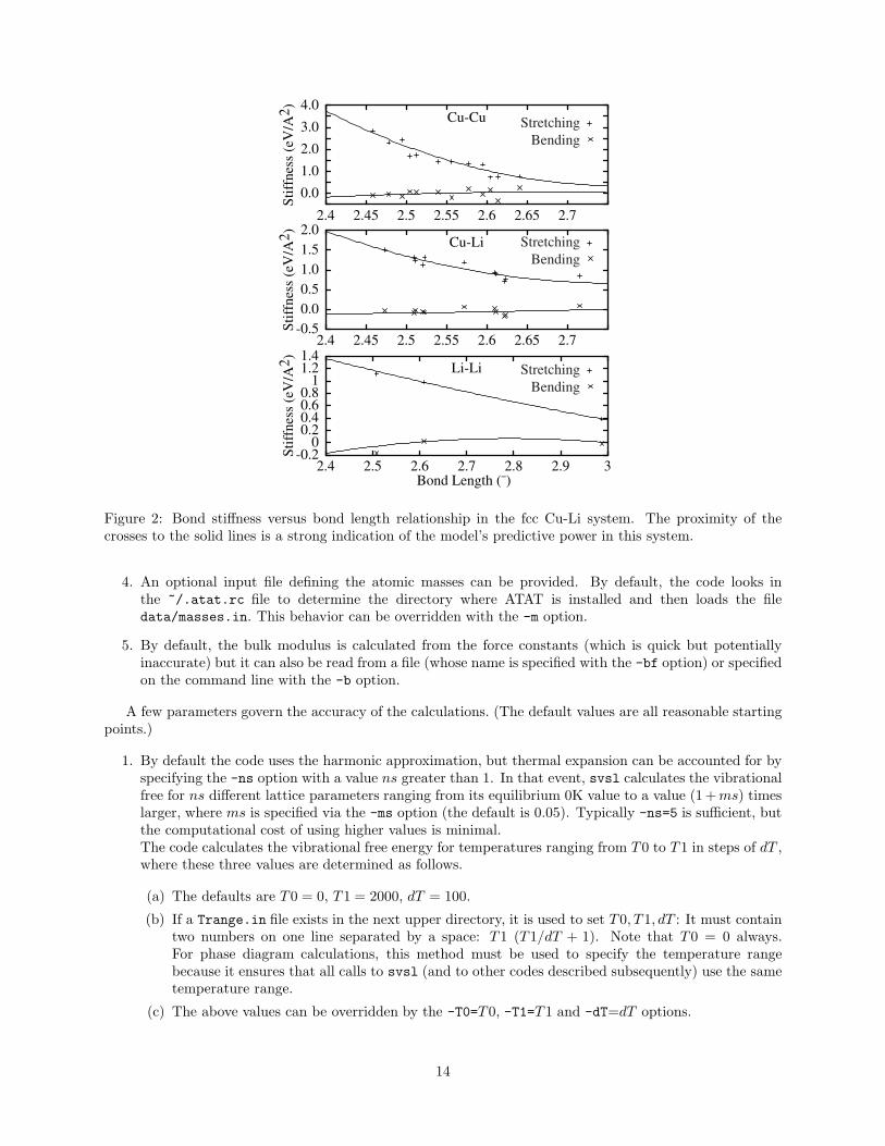
Diagnostic files are also output: The fitsvsl.log file contains all the matrices generated in the fittingprocess, including the actual forces, compared with the ones predicted by the spring model. A plot of thestiffness vs. length relationship is available in the files fitsvsl.gnu (a gnuplot script) and f *.dat the rawstiffness data to be plotted. This is helpful for assessing the validity of the transferability assumption, asillustrated in Figure 2.

Note that the fitfc and fitsvsl codes are mutually compatible: The perturbations generated with onecode can be used in a fit carried out with the other. This is useful if one realizes midway through the processthat one approach is too slow or the other too inaccurate.

Once the slspring.out file has been generated with fitsvsl, the svsl code can exploit it to rapidlypredict vibrational properties of numerous similar structures. Like fitfc, svsl is structure-specific and mustbe run within a structural directory containing the following files (three of which should now be familiar):

1. a “relaxed” structure file (str relax.out) and

2. an “unrelaxed” structure file (str.out). The latter provides the ideal atomic positions that are usedto automatically determine which atoms lie in the nearest neighbor shell. This file can be the same asthe relaxed structure but then the determination of the nearest neighbor shell may be less reliable.

3. In addition, svsl requires a transferable force constant file slspring.out. It looks for this file in thecurrent directory and, if not found, it also looks one directory up, where it would typically have beenplaced by an earlier fitsvsl command.

13A more general format for the slspring.out file then used — contact the author for more information.

13

0.0

1.0

2.0

3.0

4.0

2.4 2.45 2.5 2.55 2.6 2.65 2.7

Sti

ffnes

s (e

V/A

2)

Cu-Cu

-0.5

0.0

0.5

1.0

1.5

2.0

2.4 2.45 2.5 2.55 2.6 2.65 2.7

Sti

ffnes

s (e

V/A

2)

Cu-Li

-0.20

0.20.40.60.8

11.21.4

2.4 2.5 2.6 2.7 2.8 2.9 3

Sti

ffnes

s (e

V/A

2)

Bond Length (¯)

Li-Li

Stretching

Bending

Stretching

Bending

Stretching

Bending

Figure 2: Bond stiffness versus bond length relationship in the fcc Cu-Li system. The proximity of thecrosses to the solid lines is a strong indication of the model’s predictive power in this system.

4. An optional input file defining the atomic masses can be provided. By default, the code looks inthe ~/.atat.rc file to determine the directory where ATAT is installed and then loads the filedata/masses.in. This behavior can be overridden with the -m option.

5. By default, the bulk modulus is calculated from the force constants (which is quick but potentiallyinaccurate) but it can also be read from a file (whose name is specified with the -bf option) or specifiedon the command line with the -b option.

A few parameters govern the accuracy of the calculations. (The default values are all reasonable startingpoints.)

1. By default the code uses the harmonic approximation, but thermal expansion can be accounted for byspecifying the -ns option with a value ns greater than 1. In that event, svsl calculates the vibrationalfree for ns different lattice parameters ranging from its equilibrium 0K value to a value (1 + ms) timeslarger, where ms is specified via the -ms option (the default is 0.05). Typically -ns=5 is sufficient, butthe computational cost of using higher values is minimal.The code calculates the vibrational free energy for temperatures ranging from T 0 to T 1 in steps of dT ,where these three values are determined as follows.

(a) The defaults are T 0 = 0, T 1 = 2000, dT = 100.

(b) If a Trange.in file exists in the next upper directory, it is used to set T 0, T 1, dT : It must containtwo numbers on one line separated by a space: T 1 (T 1/dT + 1). Note that T 0 = 0 always.For phase diagram calculations, this method must be used to specify the temperature rangebecause it ensures that all calls to svsl (and to other codes described subsequently) use the sametemperature range.

(c) The above values can be overridden by the -T0=T 0, -T1=T 1 and -dT=dT options.

14

2. The k-point sampling grid is specified with the -kp=kp option. The actual number of k-points usedis at least kp divided by the number of atoms in the cell. An internal algorithm builds a k-point gridthat equalizes as much as possible the k-point density along all directions in space

The output files are as follows:

1. svsl.log : a log file giving some of the intermediate steps of the calculations in particular, the predictedbulk modulus which should be checked for accuracy.

2. vdos.out: the phonon density of states for each lattice parameter considered (unstable modes appearas negative frequencies).

3. svsl.out: gives along each row, the temperature, the free energy, and the linear thermal expansion(e.g. 0.01 means that the lattice has expansion by 1% at that temperature).

4. fvib: similar to svsl.out but gives only the free energy.

Examples of studies employing this code can be found in [34–36]

3.2 Electronic excitations

The felec code calculates the electronic free energy within the one-electron and temperature-independentbands approximations. It expects a dos.out input file containing an electronic density of states and the num-ber of electrons to populate it. This file is typically generated by the ab initio call up utilities runstuct xxxx

(see Section 6). It is rarely needed to use anything but the default option:felec -d

The output files are:

1. felec.log, containing the temperature and corresponding free energy (per unit cell) on each line.

2. felec is similar to felec.log but only contains the free energies.

3. plotdos.out contains the dos in a format suitable to be plotted, with the energy normalized so thatthe Fermi level is at 0.

It should be noted that the above approximation are not always satisfactory, notably in magnetic systems.There are two (currently experimental) magnetic free energy calculators included in ATAT:

1. fmag, which relies on a simple quantum mechanical mean field model and

2. fempmag, which implements the widely used semi-empirical method introduced in [37].

3.3 Cluster expansions of nonconfigurational free energies

The fitfc, svsl and felec codes enables the calculation of free energies of individual configuration on alattice. However, to properly calculate the free energy of system exhibiting both configurational and noncon-figurational disorder, a cluster expansion needs to be constructed to be able to predict the nonconfigurationalfree energy of any given configuration. This cluster expansion can then be provided as an input to the MonteCarlo code memc2 which will now be able to properly account for both configurational and nonconfigurationalcontributions to the free energy. Here is how to proceed.

1. First create a Trange.in file indicating the temperature range to be sampled. For instance, if onewishes to sample from 0K to 2000K in intervals of 100K, type

echo 2000 21 > Trange.in

(The lowest temperature is always 0K and note that 2000/(21− 1) = 100.)This ensures that all calls to fitfc, svsl and felec with use the same temperature range.

15

2. ATAT provides the foreachfile utility to repeat the same command in all subdirectories containinga specified file. For instance, to calculate the vibrational free energy using svsl in all structure subdi-rectories, one could type

foreachfile -e str relax.out svsl -d

This executes the svsl code with the default options (-d) in each subdirectory containing a str relax.out

file while skipping directories with an error file (-e). If desired, a similar process can be used for theelectronic free energies:foreachfile -e dos.out felec -d

3. Next, construct a cluster expansion of the vibrational free energy data contained in the */fvib files:clusterexpand fvib

Note that the files */fvib actually contain a column of numbers (one for each temperature) —clusterexpand simply produce a separate cluster expansion for each scalar element in */fvib. Bydefault, this commands reads in the clusters from the clusters.out file, as they were generated ear-lier by mmaps.14 The user has some control over which clusters to include (1) or exclude (0) via the-s=[comma-separated string of 0s and 1s] option. The user can also check if the crossvalidationscore, reported with -cv option, can be improved by changing the cluster selection. A similar expansioncan be done for electronic contributions:

clusterexpand felec

4. Finally, combine the energy cluster expansion from eci.out (generated by mmaps) with the vibrational(fvib.eci) and electronic (felec.eci) cluster expansions created in the previous step into a single“master” cluster expansion file (teci.out) that will be read by the Monte Carlo code:

mkteci fvib.eci felec.eci

For this step to succeed it is essential that all clusterexpand commands were run with the samemmaps-generated clusters.out file (although different clusters can be included or excluded with the-s option of clusterexpand without any problem).

5. Run memc2. It is often instructive to try and compare simulations that include or exclude somecomponents of the nonconfigurational free energy. To this effect, one can simply rerun mkteci withthe list of contributions to include before rerunning memc2.

Example of the use of this methodology can be found in [34–36]. For easy reference, Figure 3 shows aflowchart of the entire procedure while Figure 4 showcases a practical example of this methodology.

4 Special Quasirandom Structure generation

The use of the cluster expansion is essential to properly model nondilute alloys exhibiting configurationaldisorder with potential short-range order ([39]). However, at sufficiently high temperatures, the limitingcase of a fully random alloy provides a useful approximation. Although this limit can be calculated witha cluster expansion, it is sometimes convenient to directly determine high-temperature limiting quantitieswith a small number of supercell ab initio calculations without first constructing a cluster expansion. Theconcept of Special Quasirandom Structures (SQS) [40] provides an efficient way to take this route. AnSQS represents the best periodic supercell approximation to the true disordered state for a given numberof atoms per supercell. The quality of an SQS is measured in terms of the number of correlations of thefully disordered state it is able to match exactly. Typically, one attempts to preferably match shorter-range correlations while gradually enlarging the supercell to extend the range of matching correlations untilconvergence of the properties of interest. Traditionally, SQS are built based on matching the pair correlations,although for best performances, multibody correlations should be considered as well. The SQS generationutility included in ATAT (gensqs) can account for any user-specified set of correlations.

The SQS generation process in ATAT (as used, for instance, in [16, 39, 41]) is as follows:

14If the user wishes to use clusterexpand without first running mmaps, a suitable clusters.out file can be generated withthe a command of the form corrdump -clus -2=[max pair radius] -3=[max triplet radius] etc. A lat.in file still needsto be supplied.

16

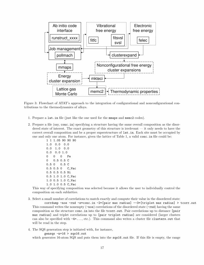
mmaps

memc2

fitfcfitsvsl

svslfelec

clusterexpand

runstruct_xxxx

pollmach

mkteci

Vibrational

free energy

Electronic

free energy

Job management

Ab initio code

interface

Energy

cluster expansion

Nonconfigurational free energy

cluster expansions

Thermodynamic propertiesLattice gas

Monte Carlo

Figure 3: Flowchart of ATAT’s approach to the integration of configurational and nonconfigurational con-tributions to the thermodynamics of alloys.

1. Prepare a lat.in file (just like the one used for the mmaps and memc2 codes).

2. Prepare a file (say, conc.in) specifying a structure having the same overall composition as the disor-dered state of interest. The exact geometry of this structure is irrelevant — it only needs to have thecorrect overall composition and be a proper superstructure of lat.in. Each site must be occupied byone and only one atom. For instance, given the lattice of Table 1, a valid conc.in file could be:

1 1 1.05 90 90 90

1.0 0.0 0.0

0.0 1.0 0.0

0.0 0.0 1.0

0 0 0 Fe

0 0.5 0.5 C

0.5 0 0.5 C

0.5 0.5 0 C,Vac

0.5 0.5 0.5 Ni

0.5 1.0 1.0 C,Vac

1.0 0.5 1.0 C,Vac

1.0 1.0 0.5 C,Vac

This way of specifying composition was selected because it allows the user to individually control thecomposition on each sublattice.

3. Select a small number of correlations to match exactly and compute their value in the disordered state:corrdump -noe -rnd -s=conc.in -2=[pair max radius] --3=[triplet max radius] > tcorr.out

This command writes the nonempty (-noe) correlations of the disordered state (-rnd) having the samecomposition as the structure conc.in into the file tcorr.out. Pair correlations up to distance [pair

max radius] and triplet correlations up to [pair triplet radius] are considered (larger clusterscan also be specified with -4=..., etc.). This command also writes a cluster file clusters.out thatwill be read in the step.

4. The SQS generation step is initiated with, for instance,gensqs -n=16 > sqs16.out

which generates 16-atom SQS and puts them into the sqs16.out file. If this file is empty, the range

17

400

600

800

1000

1200

1400

1600

0 20 40 60 80 100

T (

K)

B32

fcc

bcc

liquid

0

0.05

0.1

0.15

0 20 30 5010 40 60

emf

(V)

xLi (at %)xLi (at %)

xLi (at %)xLi (at %)

b)a)

d)c)

fcc bcc B32 B32 + liq.

first-principles

experiments

-0.4

-0.35

-0.3

-0.25

-0.2

-0.15

-0.1

0 20 40 60 80 100

fccbcc

bcc Li

Fre

e en

ergy (

eV)

T = 1000K

-0.04

-0.03

-0.02

-0.01

0

0 0.2 0.4 0.6 0.8 1

Ener

gy (

eV)

bcc

fcc

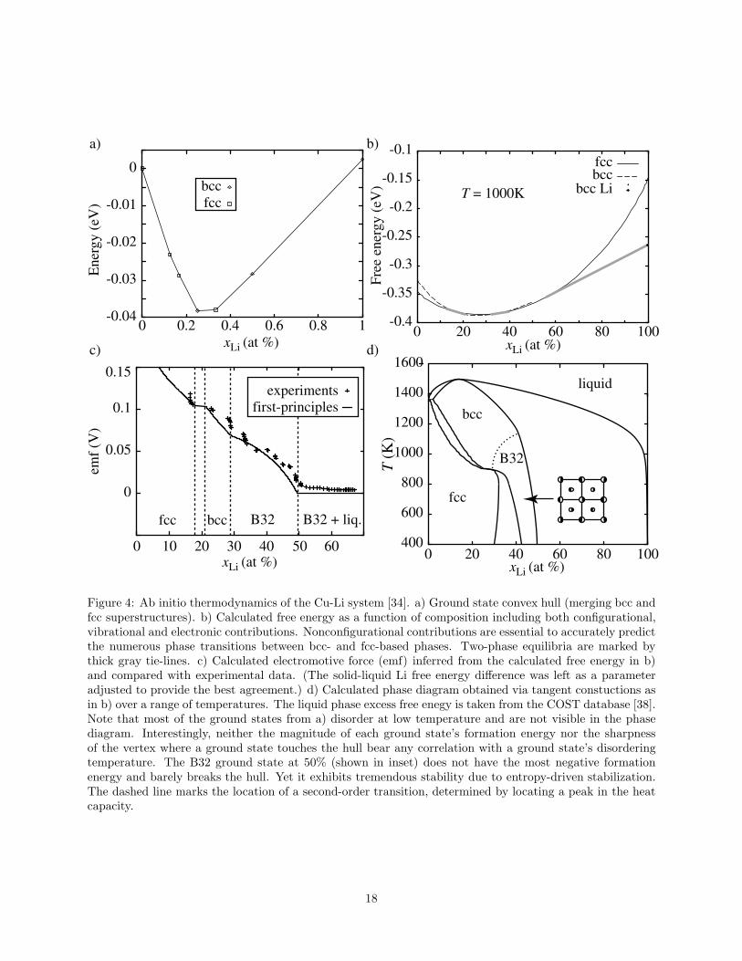
Figure 4: Ab initio thermodynamics of the Cu-Li system [34]. a) Ground state convex hull (merging bcc andfcc superstructures). b) Calculated free energy as a function of composition including both configurational,vibrational and electronic contributions. Nonconfigurational contributions are essential to accurately predictthe numerous phase transitions between bcc- and fcc-based phases. Two-phase equilibria are marked bythick gray tie-lines. c) Calculated electromotive force (emf) inferred from the calculated free energy in b)and compared with experimental data. (The solid-liquid Li free energy difference was left as a parameteradjusted to provide the best agreement.) d) Calculated phase diagram obtained via tangent constuctions asin b) over a range of temperatures. The liquid phase excess free enegy is taken from the COST database [38].Note that most of the ground states from a) disorder at low temperature and are not visible in the phasediagram. Interestingly, neither the magnitude of each ground state’s formation energy nor the sharpnessof the vertex where a ground state touches the hull bear any correlation with a ground state’s disorderingtemperature. The B32 ground state at 50% (shown in inset) does not have the most negative formationenergy and barely breaks the hull. Yet it exhibits tremendous stability due to entropy-driven stabilization.The dashed line marks the location of a second-order transition, determined by locating a peak in the heatcapacity.

18

of correlations to be matched exactly needs to be reduced in step 3. A word of caution: gensqs onlygenerates structures containing exactly the number of atoms per unit cell specified by the -n option(i.e., if an SQS with a smaller unit cell exists, it will not be listed).

5. The output file sqs16.out may contain a large number of candidate SQS. While these a match thespecified criteria, they may differ in quality in terms of the correlations not included in the screeningprocess. Further screening can be performed with the command

corrdump -2=[another radius] -3=[another radius] -4=[another radius] -noe -s=sqs16.out

which will output the correlations of all SQS in sqs16.out. Clearly, the radii specified should be largerthan in step 3 in order to distinguish and rank these SQS.

While there are no formal rules to decide whether it is preferable to match more pairs or more multi-body correlations, general guidelines can be given. In general, it would be unusual to match longer rangen-body correlations than m-body interactions if n > m. In systems exhibiting large relaxations (due to largeatomic size mismatches), multi-body correlations are expected be important, while in ionic systems, pairinteractions are expected to dominate.

SQS generation via exhaustive enumeration is time-consuming. This can be alleviated by exploitingparallelism. Multiple independent copies of gensqs can be run on separate processors if one specifiesthe -ip=[index] and -tp=[number of processes] options. The [index] runs from 0 to [number of

processes-1] and is used to tell each copy of gensqs which portion of the space to scan. For maximumefficiency, [number of processes] should be a factor of the total number of possible supercells, which canbe determined, e.g., with the gensqs -n=16 -pc command.

Another way to improve SQS generation speed is via stochastic sampling [42]. Such an approach seeksto quickly find close-to-optimal solutions rather than slowly finding an exact solution. Another approachis to scan through configurations in such as way that only the desired composition is sampled, using atompermutations rather than atom “transmutations”. This scheme becomes increasingly advantageous as onemoves away from equiatomic compositions. Yi Wang contributed a useful code implementing these twoalgorithms (that were used in [16]), which will be included in the ATAT distibution shortly.

Finally, we note that SQS prove useful in the construction of a cluster expansion as well. Any generatedSQS can be included into the set structures used to fit a cluster expansion as a way to ensure that theproperties of the disordered state are properly reproduced. In practice, one can merely place the desiredSQS into a str.out file within a subdirectory and run an ab initio code on it with runstruct xxxx. Themmaps code will readily read in any user-specified structure placed in its directory hierarchy (provided thelat.in files used in mmaps and gensqs are identical).

5 The tensorial cluster expansion

While the formalism enabling the cluster expansion of tensors has been derived in [43], we provide here abrief explanation of how to use this feature. In Section 3.3, it was shown how to cluster expand a scalar —the process is similar for tensors.

1. Create a lat.in providing the lattice and a gcetensor.in file describing the type of tensor in theform:

[rank]

[list of pairs of indices indicating which simultaneous index permutations leave

the tensor invariant]

[next list, etc...]

To fix the ideas, here are a few examples. For strain or stress the gcetensor.in should be:2

0 1 (indicating that such tensor is symmetric, i.e., εij = εji)while for elastic constants, it should be:

4

0 1 (indicating cijkl = cjikl)2 3 (indicating cijkl = cijlk)0 2 1 3 (indicating cijkl = cklij).

19

2. Generate a list of clusters with the commandgce -clus -2=[max pair radius] -3=[max triplet radius] etc.

Note that gce (which stands for Generalized Cluster Expansion) admits essentially the same syntaxas corrdump in the scalar case.

3. Calculate the property tensor associated with each structure.15 This is highly application-dependent.For instance, to calculate the static lattice strain, one could use (assuming ab initio calculations havebeen run in each subdirectory):

foreachfile -e str relax.out analrelax -d ">" strain

To calculate the elastic constants one could use:foreachfile -e str relax.out calcelas -d (this generates perturbations)pollmach -e runstruct xxxx -w force.wrap (this calculates the induced reaction stresses)foreachfile -e str relax.out calcelas -f ">" elas (this fits the elastic tensor and writes

it in the file elas.)

4. Finally, do the cluster expansion itself with:clusterexpand -pa -g strain

clusterexpand -pa -g elas

the -g invokes the generalized cluster expansion option while the -pa indicates that the quantities tobe expanded are intensive (i.e. per atom).

6 Interfaces with ab initio codes

All interfaces have the general name runstruct xxxx. Currently, the following are supported: runstruct vasp

(for the VASP code [44, 45]) runstruct abinit (for the abinit [46, 47] code), runstruct gulp (for theGULP code [48, 49]). In addition, Monodeep Chakraborty, Jurgen Spitaler, Peter Puschnig and ClaudiaAmbrosch-Draxl have written an interface with WIEN2k [50], which will be publicly available shortly. Finally,runstruct pwscf (for the PWscf code [51]) is under development.

Each interface has the following characteristics in common:

1. It reads the geometry of a structure from the str.out file in current directory, written in the ATATformat. If a str hint.out file exists, it takes precedence over the str.out file. This is useful toprovide educated guesses of the relaxed geometry via external user-supplied codes.

2. It reads some code-specific parameters from a file called xxxx.wrap (or specified with -w [file])located in the current directory or up to two levels above. This separation between the geometry andcalculation parameter input files is essential to ensure that all the pieces of ATAT are fully interoperable.

3. It runs the appropriate ab initio or atomistic code. If an argument is given to the runstruct xxxx

this string is used as prefix to the ab initio command. This feature is used to run the appropriate coderemotely without having to install ATAT on the compute nodes.

4. It writes the structure’s energy in the file energy and the structure’s relaxed geometry in str relax.out.(If no relaxations are allowed, then the unrelaxed geometry is written in str relax.out.)

5. It writes the forces acting on all atoms in forces.out, the stress acting on the cell in stress.out andthe electronic density of states in dos.out (although these are not yet implemented in all runstruct xxxx

commands).

6. If anything goes wrong with the calculations, a file called error is written.

Typically the ab initio codes are not called one run at the time but rather as a batch of many jobs. Thepollmach command manages such pools of jobs. The basic principle is simple: If a file called wait existsin a subdirectory, pollmach will find it and run the command specified on the command line within that

15This list of structures could come from a previous mmaps run, for instance, or it could be generated manually using thegenstr command.

20

directory. For instance,pollmach runstruct xxxx

will repeatedly wait for a wait file to be found, delete it, and then run runstruct xxxxwith the correspondingdirectory. In a multiprocessor environment, pollmach can simultaneously dispatch different jobs to differentprocessors. This simple mechanism allows most of the ATAT codes to be completely platform-independent,with pollmach being the only platform-dependent piece.

The first time pollmach is run, default configurational files are set up and the user will be asked totailor them to the local computing environment. The ATAT distribution includes many examples of setups,including the increasingly common case of a large pool of processors to be divided up into subgroup thateach run a separate parallel version of an ab initio code.

7 Utilities

We now briefly mention some utilities to give users direct access to some of the inner algorithms of ATAT.

1. corrdump finds symmetry operations, enumerates clusters, calculates correlations (including of thedisordered state), etc.

2. genstr enumerates superstructures of a given lattice.

3. pdef generates substitutional point defect supercells.

4. cellcvrt manipulates ATAT-formatted structure files, changing coordinate systems, converting frac-tional to cartesian coordinates, finding supercells and subcells, etc.

5. lsfit implements least-squares fitting.

6. nnshell finds nearest-neighbor shells.

7. A number of text parsing utilities: getvalue, getlines, sspp.

More information regarding these utilities can be found in their respective help files (accessed by specifyingthe -h option).

8 Conclusion

This completes this overview of the various new features added to ATAT in recent years. What’s next?Probably:

1. A tighter integration between the output of the Monte Carlo code and thermodynamic databases foruse with softwares such as Thermocalc and Pandat;

2. Material propery optimization modules exploiting the tensorial cluster expansion;

3. More automated ways to include nonconfigurational free energy;

4. Better electronic free energy calculators.

However, in large part, what will be next will depend on what users express interest in and what theauthor can get funding for. . .

21

Acknowledgements

This research was supported by the US National Science Foundation through TeraGrid resources providedby NCSA and SDSC under grant TG-DMR050013N. The NSF Center for the Science and Engineering ofMaterials at Caltech supported the preparation of this manuscript.

The author would like to thank

• Mark Asta for supporting this effort while the author was at Northwestern.

• Gerd Ceder for supporting this effort while the author was at MIT.

• Yi Wang, who has contributed an efficient SQS generator.

• Dongwong Shin, who has contributed a list of useful lattices.

• Volker Blum, who provided a nice perl remake of the load checking utility chl.

• Mayeul d’Avezac, who fixed a number of tricky compilation problems and identified a few bugs.

• Gautam Ghosh, who provided a utility to convert emc2 output files into a format suitable for theThermocalc’s Parrot module. He also suggested the inclusion of magnetic free energies based on [37].

• Zhe Liu for his contributions to generalize the Stiffness vs. Length approach to include composition-dependence.

• Monodeep Chakraborty, Jurgen Spitaler, Peter Puschnig and Claudia Ambrosch-Draxl, who are devel-oping an interface with WIEN2k.

• Ben Burton and Raymundo Arroyave, who helped debug the code and the documentation.

• Pratyush Tiwary, who proofread this manual.

These faithful and patient users (and many others) have been crucial to help maintain and develop thistoolkit.

A Correlation to concentration conversions

ATAT calculates the matrices C and X and vectors c0 and x0 in Equations (4) and (5) as follows.

1. Start enumerating all structures (in order of increasing unit cell size) while computing the point cor-relation vector ρ for each of them. Let ρ denote the corresponding point correlation vector with aconstant element appended to it. Skip any structures whose ρ is colinear with the ρ of earlier struc-tures. Terminate this step when the number of structures kept is equal to the dimension of ρ.

2. For each of the kept structures, calculate its full concentration vector x. Create a matrix A by pastingthe column vectors x just obtained side by side. Similar, create a matrix B by pasting the columnvectors ρ previously obtained. Note that B is square and invertible by construction and calculateX = AB−1.

3. All columns of X but the last provide X while the last column of X gives x0.

4. Eliminating all colinear rows from X gives C while eliminating the corresponding elements of x0 givesc0. (Note: in ATAT, c0 is just set to zero since this makes no difference for convex hull construction.But x0 is fully calculated.)

22

References

[1] A. van de Walle, M. Asta, G. Ceder, The Alloy Theoretic Automated Toolkit: A user guide, CALPHADJournal 26 (2002) 539.

[2] A. van de Walle, G. Ceder, Automating first-principles phase diagram calculations, Journal of PhaseEquilibria 23 (2002) 348.

[3] A. van de Walle, M. Asta, Self-driven lattice-model monte carlo simulations of alloy thermodynamicproperties and phase diagrams, Modelling Simul. Mater. Sci. Eng. 10 (2002) 521.

[4] J. M. Sanchez, F. Ducastelle, D. Gratias, Generalized cluster description of multicomponent systems,Physica 128A (1984) 334.

[5] F. Ducastelle, Order and Phase Stability in Alloys, Elsevier Science, New York, 1991.

[6] D. de Fontaine, Cluster approach to order-disorder transformation in alloys, Solid State Phys. 47 (1994)33.

[7] A. Zunger, First principles statistical mechanics of semiconductor alloys and intermetallic compounds,in: P. E. Turchi, A. Gonis (Eds.), NATO ASI on Statics and Dynamics of Alloy Phase Transformation,Vol. 319, Plenum Press, New York, 1994, p. 361.

[8] A. Zunger, Spontaneous atomic ordering in semiconductor alloys: Causes, carriers, and consequences,MRS Bull. 22 (1997) 20.

[9] C. Wolverton, V. Ozolins, A. Zunger, Short-range-order types in binary alloys: a reflection of coherentphase stability, J. Phys.: Condens. Matter 12 (2000) 2749.

[10] G. Ceder, A. van der Ven, C. Marianetti, D. Morgan, First-principles alloy theory in oxides, ModellingSimul. Mater Sci Eng. 8 (2000) 311.

[11] M. Asta, V. Ozolins, C. Woodward, A first-principles approach to modeling alloy phase equilibria, JOM- Journal of the Minerals Metals & Materials Society 53 (2001) 16.

[12] A. C. Powell, R. Arroyave, Open source software for materials and process modeling, JOM 60 (2008)32.

[13] P. D. Tepesch, G. D. Garbulsky, G. Ceder, Model for configurational thermodynamics in ionic systems,Phys. Rev. Lett. 74 (1995) 2272.

[14] A. van de Walle, D. Ellis, First-principles thermodynamics of coherent interfaces in samarium-dopedceria nanoscale superlattices, Phys. Rev. Lett. 98 (2007) 266101.

[15] G. Ghosh, A. van de Walle, M. Asta, First-principles phase stability calculations of pseudobinary alloysof (Al,Zn)3Ti with L12, DO22 and DO23 structures, Journal of Phase Equilibria and Diffusion 28 (2007)9.

[16] D. Shin, A. van de Walle, Y. Wang, Z.-K. Liu, First-principles study of ternary fcc solution phases fromspecial quasirandom structures, Phys. Rev. B 76 (2007) 144204.

[17] A. van de Walle, G. Ceder, The effect of lattice vibrations on substitutional alloy thermodynamics, Rev.Mod. Phys. 74 (2002) 11.

[18] G. Ceder, A derivation of the Ising model for the computation of phase diagrams, Comput. Mater. Sci.1 (1993) 144.

[19] S. Wei, M. Y. Chou, Ab initio calculation of force constants and full phonon dispersions, Phys. Rev.Lett. 69 (1992) 2799.

23

[20] G. D. Garbulsky, G. Ceder, Contribution of the vibrational free energy to phases stability in substitu-tional alloys: methods and trends, Phys. Rev. B 53 (1996) 8993.

[21] S. Baroni, P. Giannozzi, A. Testa, Green’s-function approach to linear response in solids, Phys. Rev.Lett. 58 (18) (1987) 1861.

[22] P. Giannozzi, S. de Gironcoli, P. Pavone, S. Baroni, Ab initio calculation of phonon dispersions insemiconductors, Phys. Rev. B 43 (1991) 7231.

[23] X. Gonze, D. C. Allan, M. P. Teter, Dielectric tensor, effective charges, and phonons in α-quartz byvariational density-functional perturbation theory, Phys. Rev. Lett. 68 (1992) 3603.

[24] X. Gonze, First-principles responses of solids to atomic displacements and homogeneous electric fields:Implementation of a conjugate-gradient algorithm, Phys. Rev. B 55 (1997) 10337.

[25] X. Gonze, C. Lee, Dynamical matrices, born effective charges, dielectric permittivity tensors, and in-teratomic force constants from density-functional perturbation theory, Phys. Rev. B 55 (1997) 10355.

[26] S. de Gironcoli, Lattice dynamics of metals from density-functional perturbation theory, Phys. Rev. B51 (1995) 6773.

[27] A. van de Walle, G.Ceder, First-principles computation of the vibrational entropy of ordered and dis-ordered Pd3V, Phys. Rev. B 61 (2000) 5972.

[28] D. Morgan, A. van de Walle, G. Ceder, J. D. Althoff, D. de Fontaine, Vibrational thermodynamics:coupling of chemical order and size effects, Modelling Simul. Mater Sci Eng. 8 (2000) 295.

[29] E. Wu, G. Ceder, A. van de Walle, Using bond-length-dependent transferable force constants to predictvibrational entropies in Au-Cu, Au-Pd, and Cu-Pd alloys, Phys. Rev. B 67 (2003) 134103.

[30] J. Z. Liu, G. Ghosh, A. van de Walle, M. Asta, Transferable force-constant modeling of vibrationalthermodynamic properties in fcc-based Al-TM (TM = Ti, Zr, Hf) alloys, Phys. Rev. B 75 (2007)104117.

[31] R. Benedek, A. van de Walle, Reaction free energies of acid attack of lithium cobaltate, Journal of theElectrochemical Society 155 (2008) A711.

[32] R. Benedek, M. M. Thackeray, A. van de Walle, Reaction free energy for proton-lithium ion exchangein lithium battery cathode materials, Chem. Mater. 20 (2008) 5485.

[33] R. Arroyave, A. van de Walle, Z.-K. Liu, First-principles calculations of the Zn-Zr system, Acta Mate-rialia 54 (2006) 473.

[34] A. van de Walle, Z. Moser, W. Gasior, First-principles calculation of the Cu-Li phase diagram, Archivesof Metallurgy and Materials 49 (2004) 535.

[35] B. Burton, A. van de Walle, U. Kattner, First principles phase diagram calculations for the wurtzite-structure systems AlN-GaN, AlN-InN and GaN-InN, J. Appl. Phys. 100 (2006) 113528.

[36] B. Burton, A. van de Walle, First principles phase diagram calculations for the system NaCl-KCl: therole of excess vibrational entropy., Chemical Geology 225 (2006) 222.

[37] I. Ohnuma, H. Enoki, O. Ikeda, R. Kainuma, H. Ohtani, B. Sundman, K. Ishida, Phase equilibria inthe fe-co binary system, Acta Materialia 50 (2002) 379.

[38] N. Saunders, COST 537 Thermochemical database for light metal alloys, in: I. Ansara, A. Dindail,M. Rand (Eds.), COST 537 Thermochemical database for light metal alloys, Vol. 2, European Commu-nities, 1998, p. 168.

24

[39] G. Ghosh, A. van de Walle, M. Asta, First-principles calculations of properties of bcc, fcc and hcp solidsolutions in Al-TM (TM = Ti, Zr, Hf) systems: A comparison between cluster expansion and supercellmethods, Acta Mater.In press.

[40] A. Zunger, S.-H. Wei, L. Ferreira, J. E. Bernard, Special quasirandom structures, Phys. Rev. Lett.65 (3) (1990) 353.

[41] D. Shin, R. Arroyave, Z.-K. Liu, A. V. de Walle, Thermodynamic properties of binary hcp solutionphases from special quasirandom structures, Phys. Rev. B 74 (2006) 024204.

[42] I. A. Abrikosov, S. I. Simak, B. Johansson, A. V. Ruban, H. L. Skriver, Locally self-consistent green’sfunction approach to the electronic structure problem, Phys. Rev. B 56 (1997) 9319.

[43] A. van de Walle, A complete representation of structure-property relationships in crystals, NatureMaterials 7 (2008) 455.

[44] G. Kresse, J. Furthmuller, Efficient iterative schemes for ab initio total-energy calculations using aplane-wave basis set, Phys. Rev. B 54 (1996) 11169.

[45] G. Kresse, J. Furthmuller, Efficiency of ab-initio total energy calculations for metals and semiconductorsusing a plane-wave basis set, Comput. Mater. Sci. 6 (1996) 15.

[46] X. Gonze, J.-M. Beuken, R. Caracas, F. Detraux, M. Fuchs, G.-M. Rignanese, L. Sindic, M. Verstraete,G. Zerah, F. Jollet, M. Torrent, A. Roy, M. Mikami, P. Ghosez, J.-Y. Raty, D. Allan, First-principlescomputation of material properties : the abinit software project, Comput. Mater. Sci. 25 (2002) 478.

[47] X. Gonze, G.-M. Rignanese, M. Verstraete, J.-M. Beuken, Y. Pouillon, R. Caracas, F. Jollet, M. Torrent,G. Zerah, M. Mikami, P. Ghosez, M. Veithen, J.-Y. Raty, V. Olevano, F. Bruneval, L. Reining, R. Godby,G. Onida, D. Hamann, D. Allan., A brief introduction to the abinit software package, Zeit. Kristallogr.220 (2005) 558.

[48] J. D. Gale, A. L. Rohl, The general utility lattice program, Mol. Simul. 29 (2003) 291.

[49] J. D. Gale, GULP - a computer program for the symmetry adapted simulation of solids, JCS FaradayTrans. 93 (1997) 629.

[50] P. Blaha, K. Schwarz, G. Madsen, D. Kvasnicka, J. Luitz, WIEN2k, http://www.wien2k.at/.

[51] P. Giannozzi, et al., Quantum-espresso, http://www.quantum-espresso.org and http://www.pwscf.org(2008).

25