Embed Size (px)
Citation preview

MULTICOMPONENT 3D SEISMIC INTERPRETATION
OF THE MARCELLUS SHALE BRADFORD COUNTY, PENNSYLVANIA
A Thesis Presented to
the Faculty of the Department of Earth & Atmospheric Sciences
University of Houston
In Partial Fulfillment
of the Requirements for the Degree
Master of Science
By
Mouna Gargouri
August 2012
ii
Multicomponent 3D seismic interpretation of the Marcellus shale, Bradford County
Pennsylvania
_______________________________
Mouna Gargouri
APPROVED:
_______________________________
Dr. Robert R. Stewart
_______________________________
Dr. C. Liner
_______________________________
Dr. James E. Gaiser
_______________________________
DEAN OF COLLEGE OF NATURAL SCIENCES AND MATHEMATICS
iii
MULTICOMPONENT 3D SEISMIC INTERPRETATION
OF THE MARCELLUS SHALE BRADFORD COUNTY, PENNSYLVANIA
An Abstract Presented to
the Faculty of the Department of Earth & Atmospheric Sciences
University of Houston
In Partial Fulfillment
of the Requirements for the Degree
Master of Science
By
Mouna Gargouri
August 2012
iv
Abstract
High spatial variability of petrophysical and petrochemical properties of the
Marcellus formation was reported by Hill et al. (2002). This creates a major challenge
in reservoir characterization with conventional seismic data. An investigation into the
potential of integrated compressional P-wave and converted-wave seismic
interpretation, to help characterize geological properties of the Devonian Marcellus
shale, has been conducted based on the 3C- 3D data set acquired. Synthetic and real
seismic data have been used to conduct this evaluation. Interval Vp/Vs analysis has
been performed and the Poisson’s ratio was generated to map lateral changes in
lithology and rock properties. Sweet spots are interpreted to area with high quartz, an
anomalous low Vp/Vs. The Vp/Vs Marcellus map shows the lateral lithological
variability and therefore brittle areas. An inversion was run for the compressional P
and the converted PS sections to examine the anomalies observed within the Vp/Vs
map. The anomalies distinguished within the Vp/Vs map were noticeable in the
inversion sections. The inversion was followed by a seismic attribute analysis to
understand the distribution of fractures. The curvature and the coherency attributes
delivered highly fractured area and major faults. This study documents the results of
an integrated workflow of seismic interpretation, seismic inversion and seismic
attribute analysis. It illustrates the potential of the Vp/Vs analysis to discriminate
between shale-rich and sand-rich material and the ability of the curvature and
coherency attribute to potentially highlight zones of intense fracturing.
v
TABLE OF CONTENTS
CHAPTER 1 INTRODUCTION ................................................................................................... 1
CHAPTER 2 BACKGROUND AND PRODUCTION HISTORY ............................................... 4
2.1 Background..................................................................................................................................................................... 4
2.2 Marcellus production history ................................................................................................................................. 9
CHAPTER 3 METHODOLOGY ................................................................................................ 11
3.1 Seismic and well log data set ................................................................................................................................ 11
3.2 Methodology ................................................................................................................................................................ 14
CHAPTER 4 RESULTS .............................................................................................................. 17
4.1 Results from previous studies .............................................................................................................................. 17
4.2 Well log interpretation ............................................................................................................................................ 18
4.3 Brittleness Index ........................................................................................................................................................ 21
4.4 Vp/Vs estimation workflow .................................................................................................................................. 23
4.4.1 Synthetic seismograms modeling ................................................................................................................ 24
4.4.2 PP and PS seismic interpretation ................................................................................................................. 29
4.4.2.1 PP and PS seismic interpretation of the top of the Marcellus ........................................................................... 30
4.4.2.2 PP and PS seismic interpretation of the base of the Marcellus ......................................................................... 32
vi
4.4.3 PP and PS isochrons .......................................................................................................................................... 33
4.4.4 Interval Vp/Vs estimation ............................................................................................................................... 35
4.5 Poisson’s ratio estimation ...................................................................................................................................... 40
4.6 Seismic attributes ...................................................................................................................................................... 43
4.6.1 Coherency attribute .......................................................................................................................................... 44
4.6.1.1 Coherency attribute at the top of the Marcellus ..................................................................................................... 44
4.6.1.2 Coherency attribute at the base of the Marcellus .................................................................................................. 46
4.6.2 Curvature attribute ........................................................................................................................................... 47
4.6.2.1 Curvature attribute at the top of the Marcellus ....................................................................................................... 48
4.6.2.2 Curvature attribute at the base of the Marcellus .................................................................................................... 50
4.7 Fold map calculations .............................................................................................................................................. 53
4.8 Post–stack seismic inversion ................................................................................................................................ 60
CHAPTER 5 FUTURE WORK ................................................................................................... 72
CHAPTER 6 CONCLUSION ...................................................................................................... 71
CHAPTER 7 APPENDIX ............................................................................................................ 74
CHAPTER 8 REFERENCES ...................................................................................................... 78
vii
LIST OF FIGURE
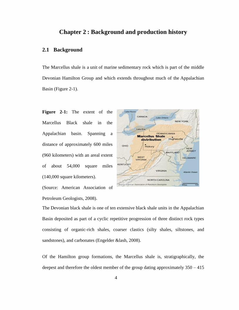
Figure 2-1: The extent of the Marcellus Black shale in the Appalachian basin. ................................................... 4
Figure 2-2: Stratigraphic column for the middle Devonian Marcellus .................................................................... 5
Figure 2-3: Marcellus shale depositional setting.
(http://www.wvsoro.org/resources/marcellus/RamsayBarrett-Shale.pdf) ......................................................... 6
Figure 2-4: The J1 and J2 regional joint sets. The J1 has an orientation East-Northeast (about
N75E) and the J2 is orthogonal to and crosscuts the first set. ...................................................................................... 8
Figure 3-1: The well logs available within the study area. The location of the well is shown in
Figure 3-2. ....................................................................................................................................................................................... 11
Figure 3-2: Location of the study area. The green rectangle represents the 3D- 3C survey in
Bradford County Northeastern Pennsylvania and the red dot represents the location of the available
well. .................................................................................................................................................................................................... 12
Figure 3-3: A zoom in of the Bradford 3C - 3D survey design map (Geokinetics). ............................................. 13
Figure 4-1: Time seismic section showing the top of the three units of the Marcellus at the well
location. The green line represents the well and the white log corresponds to the gamma Ray log. ......... 17
Figure 4-2: The well location map ....................................................................................................................................... 18
Figure 4-3: The well logs used for the interpretation ................................................................................................... 20
Figure 4-4: The well tie of the PP seismic time section a) the correlation between the synthetic
seismograms and the seismic data by matching the events on the synthetic traces (blue traces) and
the composite traces (red traces). The black traces correspond to the actual seismic data; b) the
statistically extracted wavelet with a constant phase; c) the frequency spectrum of the wavelet. ............. 27
Figure 4-5: The well tie of the PS seismic time section a) the correlation between the synthetic
seismograms and the seismic data by matching the events on the synthetic traces (blue traces) and
the composite traces (red traces). The black traces correspond to the actual seismic data; b) the
statistically extracted wavelet with a constant phase; c) the frequency spectrum of the wavelet. ............. 28
viii
Figure 4-6: PP and PS seismic time sections displaying the top and the base of the Marcellus. .................. 29
Figure 4-7: Time structure map at the top of the Marcellus for the PP seismic time section. ..................... 30
Figure 4-8: Time structure map at the top of the Marcellus for the PS seismic time section........................ 31
Figure 4-9: Time structure map at the base of the Marcellus for the PP seismic time section. .................... 32
Figure 4-10: Time structure map at the base of the Marcellus for the PS seismic time section. ................. 33
Figure 4-11: Isochrons between the top and the base of the Marcellus for the compressional wave
data. ................................................................................................................................................................................................... 34
Figure 4-12: Isochrons between the top and the base of the Marcellus for the converted wave data. ..... 35
Figure 4-13: Vp/Vs distribution map estimated from the compressional and the converted wave
data for the interval between the top and the base of the Marcellus shale. .......................................................... 38
Figure 4-14: Poisson’s ratio distribution map extracted from the interval Vp/Vs estimated from the
compressional and the converted wave data for the Marcellus Formation. ......................................................... 41
Figure 4-15: Coherency attribute at the top of the Marcellus corresponding to the PP interpreted
section. .............................................................................................................................................................................................. 45
Figure 4-16: Coherency attribute at the top of the Marcellus corresponding to the PS interpreted
section. .............................................................................................................................................................................................. 45
Figure 4-17: Coherency attribute at the base of the Marcellus corresponding to the PP interpreted
section. .............................................................................................................................................................................................. 46
Figure 4-18: Coherency attribute at the base of the Marcellus corresponding to the PS interpreted
section. .............................................................................................................................................................................................. 47
Figure 4-19: Curvature attribute at the top of the Marcellus corresponding to the PP interpreted
section. .............................................................................................................................................................................................. 49
Figure 4-20: Curvature attribute at the top of the Marcellus corresponding to the PS interpreted
section. .............................................................................................................................................................................................. 49
Figure 4-21: Curvature attribute at the base of the Marcellus corresponding to the PP interpreted
section. .............................................................................................................................................................................................. 51
ix
Figure 4-22: Curvature attribute at the base of the Marcellus corresponding to the PS interpreted
section ............................................................................................................................................................................................... 51
Figure 4-23: Brick pattern survey design .......................................................................................................................... 54
Figure 4-24: Bin fold map for the Bradford 3C- 3D survey at 3000km depth and using a bin grid of
100ft*100ft ...................................................................................................................................................................................... 56
Figure 4-25: Histogram of azimuth .................................................................................................................................... 57
Figure 4-26: Histogram of offset ........................................................................................................................................... 58
Figure 4-27: Rose diagram of offset versus azimuth .................................................................................................... 59
Figure 4-28: Model-based inversion flowchart (modified from Russell, 1988) .................................................. 62
Figure 4-29: P-impedance model applied for the P-wave data ................................................................................ 65
Figure 4-30: P-impedance model applied for the PS-wave data .............................................................................. 66
Figure 4-31: The location of the inline shown in the inversion (inline 5978) ..................................................... 67
Figure 4-32: P-wave impedance (results of the model based inversion). ............................................................. 68
Figure 4-33: PS-wave impedance (results of the model based inversion) ............................................................ 69
Figure 6-1: Workflow chart for impedance derived Vp/Vs estimation ................................................................. 73

x
LIST OF TABLES
Table 2-1: : A few of Chesapeake most notable wells from the second quarter 2010 ...................................... 10
Table 3-1: Survey Design for Bradford 3D3C Project ................................................................................................... 13
Table 4-1: Brittleness Index of some producing shale plays in the United States .............................................. 22
1
Chapter 1 Introduction
Shale represents around 75% of most sedimentary basins (Sayers, 1994) and is
primarily thought of as the hydrocarbon source rock. However, shale is now also
considered to be a reservoir (unconventional resource) and is becoming increasingly
an important exploration and production target.
Unconventional resources differ from conventional resources in that they are regional
stratigraphic accumulations of hydrocarbons which commonly occur as laterally
extensive, blanket-like sedimentary deposits (Elmira, 2008). Unlike conventional
resources, these unconventional resources are not broken into discrete fields
dependent on the trapping configurations needed to accumulate hydrocarbons.
Instead, unconventional resources are regionally continuous accumulations of organic
matter that generate hydrocarbons. In short, an unconventional resource acts as its
own source rock, reservoir, and trap.
The Marcellus shale is one example of a classic unconventional resource. It spans a
distance of approximately 600 miles (960 kilometers) with an areal extent of about
54,000 square miles (140000 square kilometers). It is present in much of the
Appalachian Basin, in an area that extends from New York generally southwestward
through Pennsylvania, Maryland, Ohio, West Virginia, and eastern Kentucky, into
Tennessee. It is said to be the largest shale-gas deposit in the world, containing about
500 TCF of recoverable gas (Engelder et al., 2009).
2
The Marcellus shale has been one of the most sought-after shale-gas resource plays in
the USA.
Characterization of gas-shale reservoirs is challenged by its highly heterogeneous
nature. The complexity stems from the natural geological variation of the rock itself.
Its properties change significantly.
The Devonian gas shales are regional accumulations having variable production
characteristics. They exhibit low matrix porosity and such a low permeability that gas
does not flow economically unless it contains high-permeability fractures, either
natural or man-made. ‘These natural fractures can be caused by tectonic forces,
desiccation and hydrocarbon generation while the process of hydraulic fracturing
stimulates and induces fractures’ (Hay and Sondergeld, 2012). Elastic properties are
necessary in locating these fractures sets. However, the mineralogical variability of
shale causes considerable variation in the elastic properties.
Traditionally, the exploration of gas shales ignores the application of the conventional
seismic because of the low reflectivity of the compressional waves when
encountering gas-saturated sections. The 3C-3D seismic survey brings the
opportunity to analyze the compressional and the shear-wave velocities.
Multicomponent seismic analysis plays an important role in the characterization of
shale gas reservoirs delivering the Vp/Vs value, which in its turn highlights the
distribution of brittleness this can help locating areas with high reservoir quality,
sweet spots, that are needed for an optimum positioning of the wells.

3
This research focuses on the application of the multicomponent seismic technique to
develop a method for Vp/Vs estimation from compressional and converted-wave
data. The main objective of this study is to delineate prospects based on the
seismically derived attribute Vp/Vs.
4
Chapter 2 : Background and production history
2.1 Background
The Marcellus shale is a unit of marine sedimentary rock which is part of the middle
Devonian Hamilton Group and which extends throughout much of the Appalachian
Basin (Figure 2-1).
The Devonian black shale is one of ten extensive black shale units in the Appalachian
Basin deposited as part of a cyclic repetitive progression of three distinct rock types
consisting of organic-rich shales, coarser clastics (silty shales, siltstones, and
sandstones), and carbonates (Engelder &lash, 2008).
Of the Hamilton group formations, the Marcellus shale is, stratigraphically, the
deepest and therefore the oldest member of the group dating approximately 350 – 415
Figure 2-1: The extent of the
Marcellus Black shale in the
Appalachian basin. Spanning a
distance of approximately 600 miles
(960 kilometers) with an areal extent
of about 54,000 square miles
(140,000 square kilometers).
(Source: American Association of
Petroleum Geologists, 2008).
5
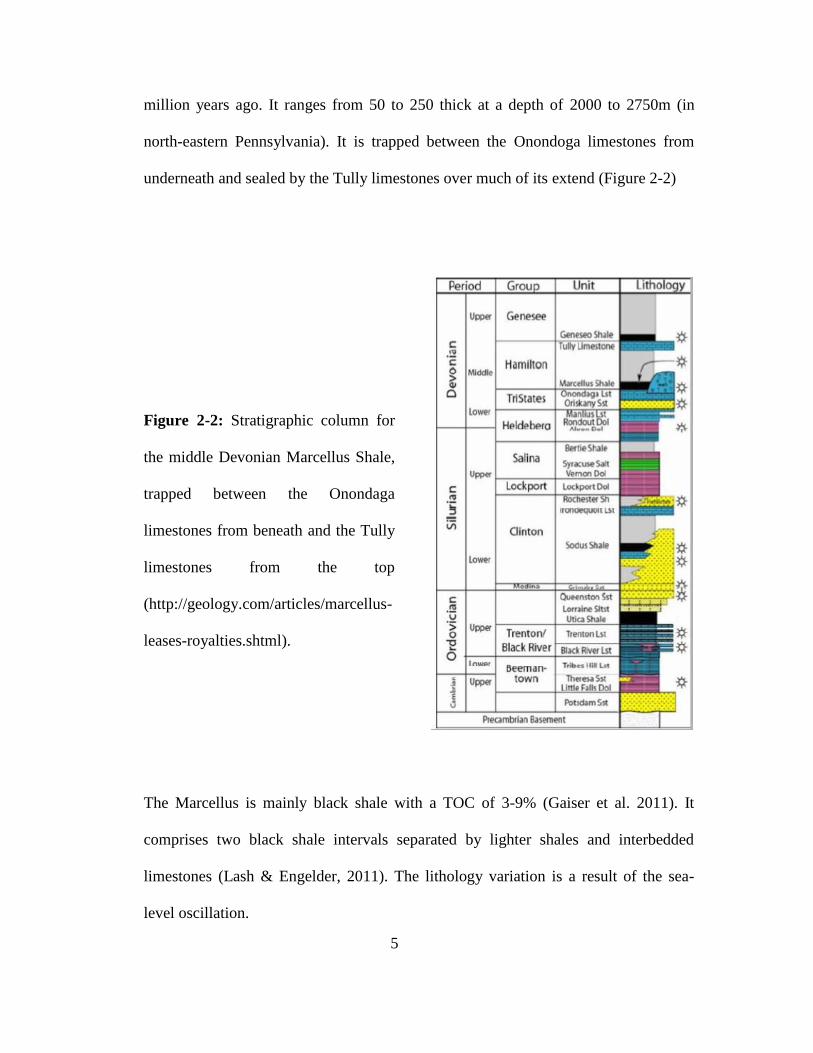
million years ago. It ranges from 50 to 250 thick at a depth of 2000 to 2750m (in
north-eastern Pennsylvania). It is trapped between the Onondoga limestones from
underneath and sealed by the Tully limestones over much of its extend (Figure 2-2)
The Marcellus is mainly black shale with a TOC of 3-9% (Gaiser et al. 2011). It
comprises two black shale intervals separated by lighter shales and interbedded
limestones (Lash & Engelder, 2011). The lithology variation is a result of the sea-
level oscillation.
Figure 2-2: Stratigraphic column for
the middle Devonian Marcellus Shale,
trapped between the Onondaga
limestones from beneath and the Tully
limestones from the top
(http://geology.com/articles/marcellus-
leases-royalties.shtml).
6
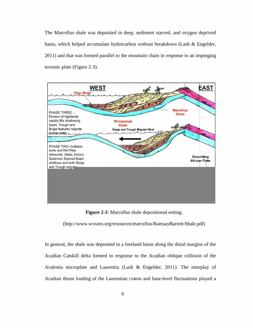
The Marcellus shale was deposited in deep, sediment starved, and oxygen deprived
basin, which helped accumulate hydrocarbon without breakdown (Lash & Engelder,
2011) and that was formed parallel to the mountain chain in response to an impinging
tectonic plate (Figure 2-3).
In general, the shale was deposited in a foreland basin along the distal margins of the
Acadian Catskill delta formed in response to the Acadian oblique collision of the
Avalonia microplate and Laurentia (Lash & Engelder, 2011). The interplay of
Acadian thrust loading of the Laurentian craton and base-level fluctuations played a
Figure 2-3: Marcellus shale depositional setting.
(http://www.wvsoro.org/resources/marcellus/RamsayBarrett-Shale.pdf)
7
first-order role in shaping the Marcellus stratigraphy creating accommodation space
(proximal trough) for its accumulation. The end of the collision marked a shallowing
of the anoxic basin filled rapidly with sediments eroded from the highlands (Lash &
Engelder, 2011). This high sediment flux prevented seawater to squeeze out of the
fine-grained matrix of the black shale. The trapped water supported the accumulation
of more sediment and at the same time precluded the compaction of the pore space
causing an increase in the pore pressure, which is the origin of the abnormally high
fluid pressure in the Devonian shale. The continued burial of the Marcellus organic-
rich muds, during the Alleghanian Orogeny, associated with the temperature and
pressure increase lead to the generation of hydrocarbons. As the expulsion of
hydrocarbon wasn’t concomitant with the expansion of the pore space, the pore
pressure raised to such a magnitude, triggering cracking in order to release the
pressure. These cracks sustained growing with more and more generation of
hydrocarbon forming natural hydraulic fractures (Engelder and Lash, 2008).
The impervious limestones layers underlying and sealing the tight, poorly connected
pores of the Marcellus Formation, have trapped huge amount of natural gas in this
shale, adsorbed on mineral grains and organic matter, trapped within the pore space
and within the fissures, cracks and joints that break through the shale (Herbert and
Sudfeld, 2011). This natural gas only flows to the wellbore when penetrating a
systematic fracture set and all successful drilled wells shared that feature.
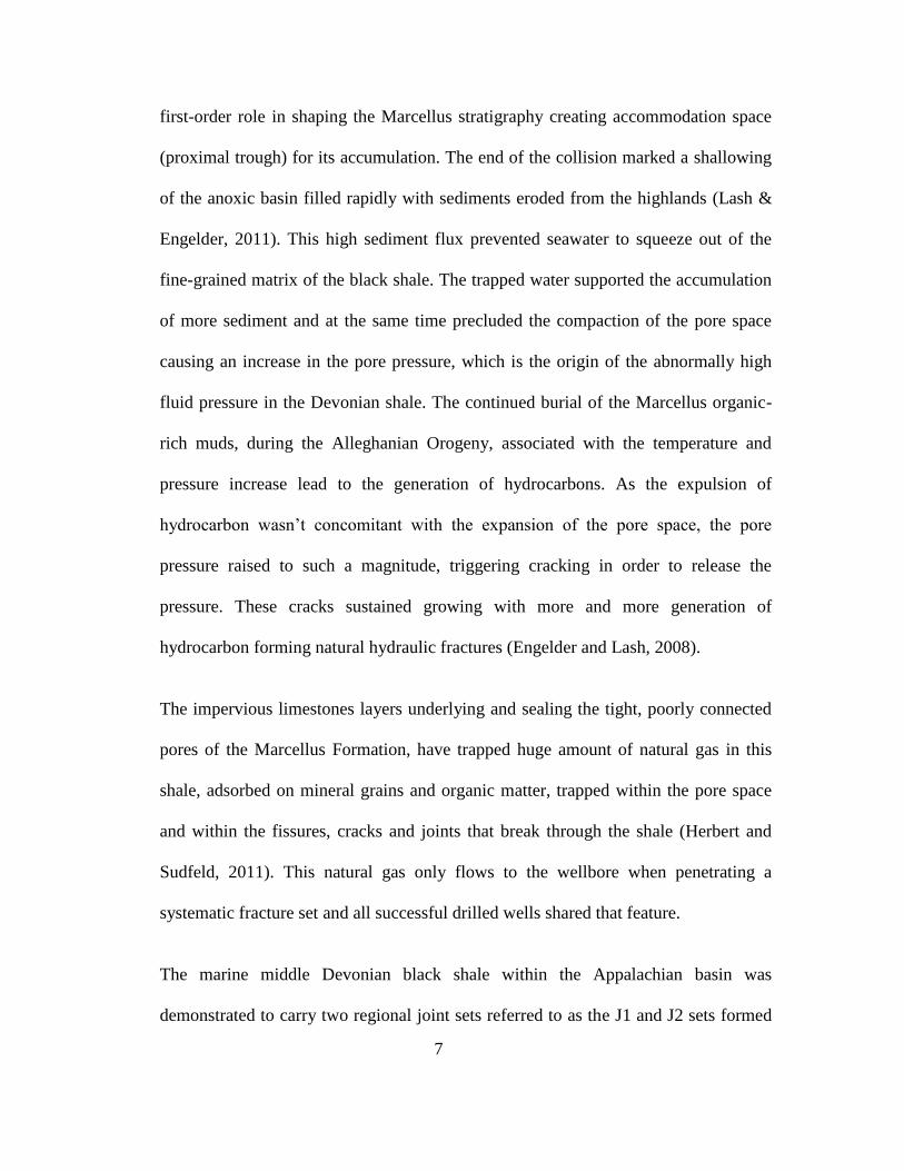
The marine middle Devonian black shale within the Appalachian basin was
demonstrated to carry two regional joint sets referred to as the J1 and J2 sets formed
8
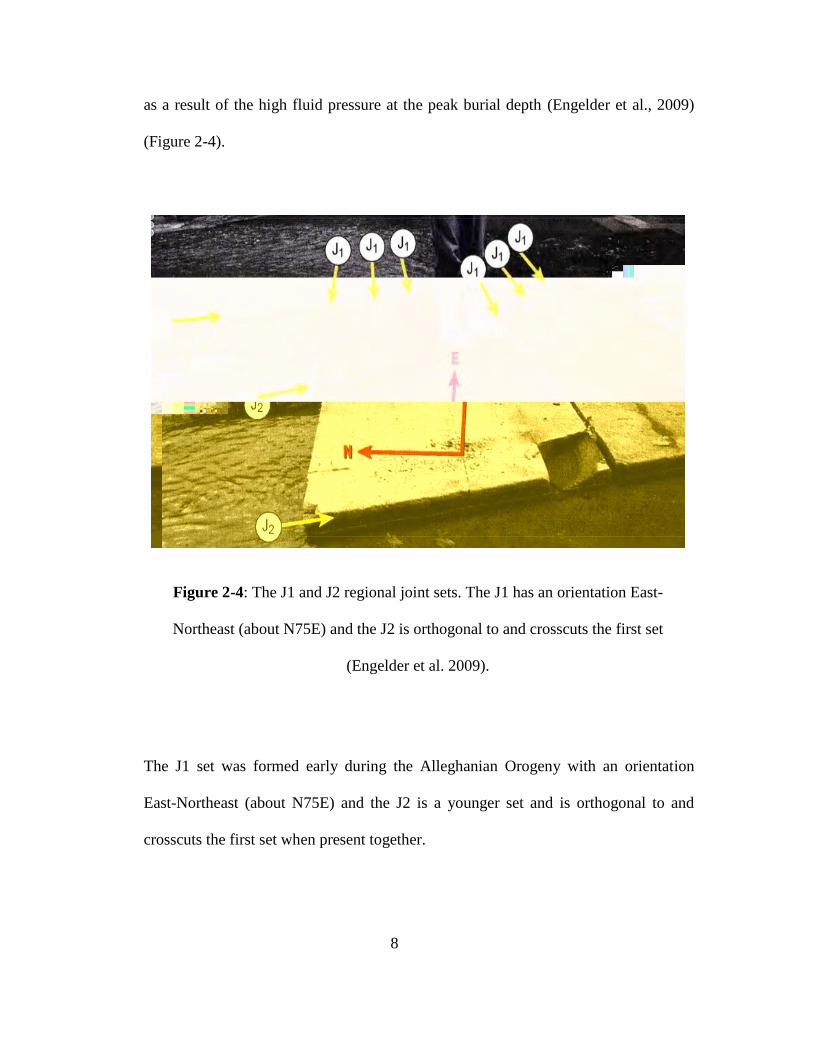
as a result of the high fluid pressure at the peak burial depth (Engelder et al., 2009)
(Figure 2-4).
The J1 set was formed early during the Alleghanian Orogeny with an orientation
East-Northeast (about N75E) and the J2 is a younger set and is orthogonal to and
crosscuts the first set when present together.
Figure 2-4: The J1 and J2 regional joint sets. The J1 has an orientation East-
Northeast (about N75E) and the J2 is orthogonal to and crosscuts the first set
(Engelder et al. 2009).
9
The first set is predominant in the black shale intervals (Engelder et al., 2009) and it
is better developed and more closely spaced compared to the J2 set which is
predominant in the lighter shale (Engelder et al., 2009). The J1 set was proved to have
almost the same direction as the maximum horizontal compressive stress of the
contemporary tectonic stress field (Engelder et al., 2009). This lead to an incorrect
conclusion that the J1 direction was controlled by the contemporary stress, which was
proved later to be a geological coincidence (Engelder et al., 2009). This parallelism
favors the propagation of the J1 hydraulic fractures set.
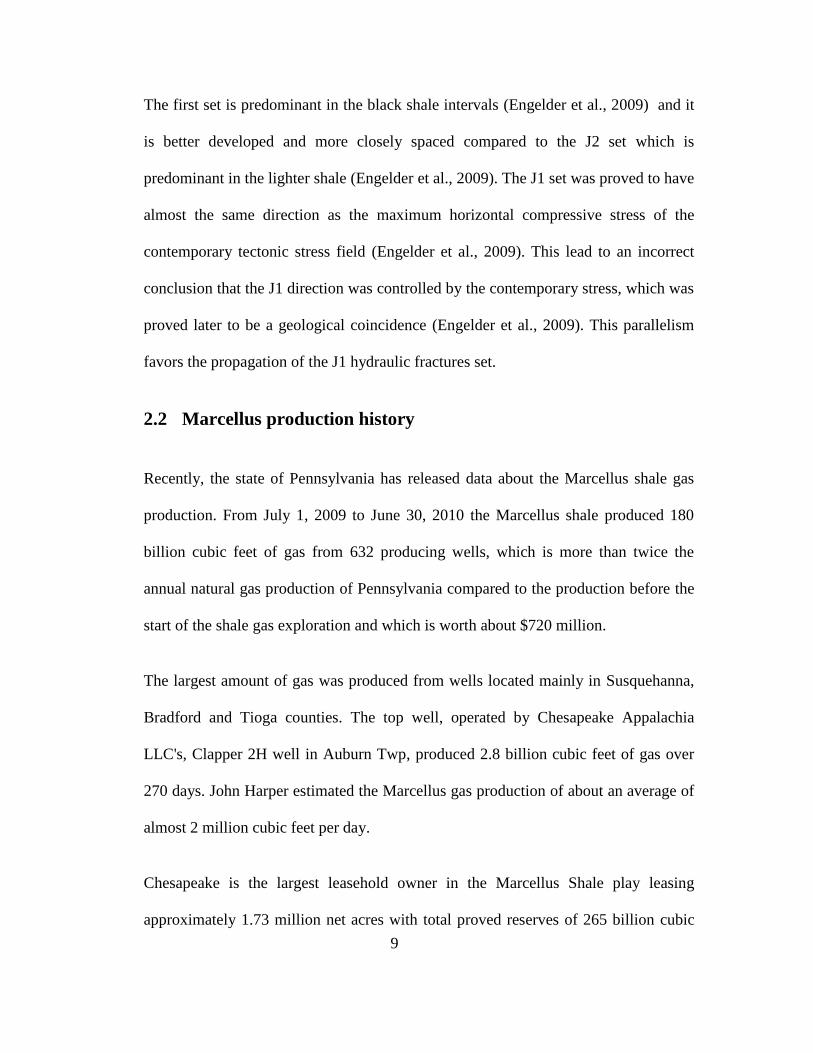
2.2 Marcellus production history
Recently, the state of Pennsylvania has released data about the Marcellus shale gas
production. From July 1, 2009 to June 30, 2010 the Marcellus shale produced 180
billion cubic feet of gas from 632 producing wells, which is more than twice the
annual natural gas production of Pennsylvania compared to the production before the
start of the shale gas exploration and which is worth about $720 million.
The largest amount of gas was produced from wells located mainly in Susquehanna,
Bradford and Tioga counties. The top well, operated by Chesapeake Appalachia
LLC's, Clapper 2H well in Auburn Twp, produced 2.8 billion cubic feet of gas over
270 days. John Harper estimated the Marcellus gas production of about an average of
almost 2 million cubic feet per day.
Chesapeake is the largest leasehold owner in the Marcellus Shale play leasing
approximately 1.73 million net acres with total proved reserves of 265 billion cubic
10
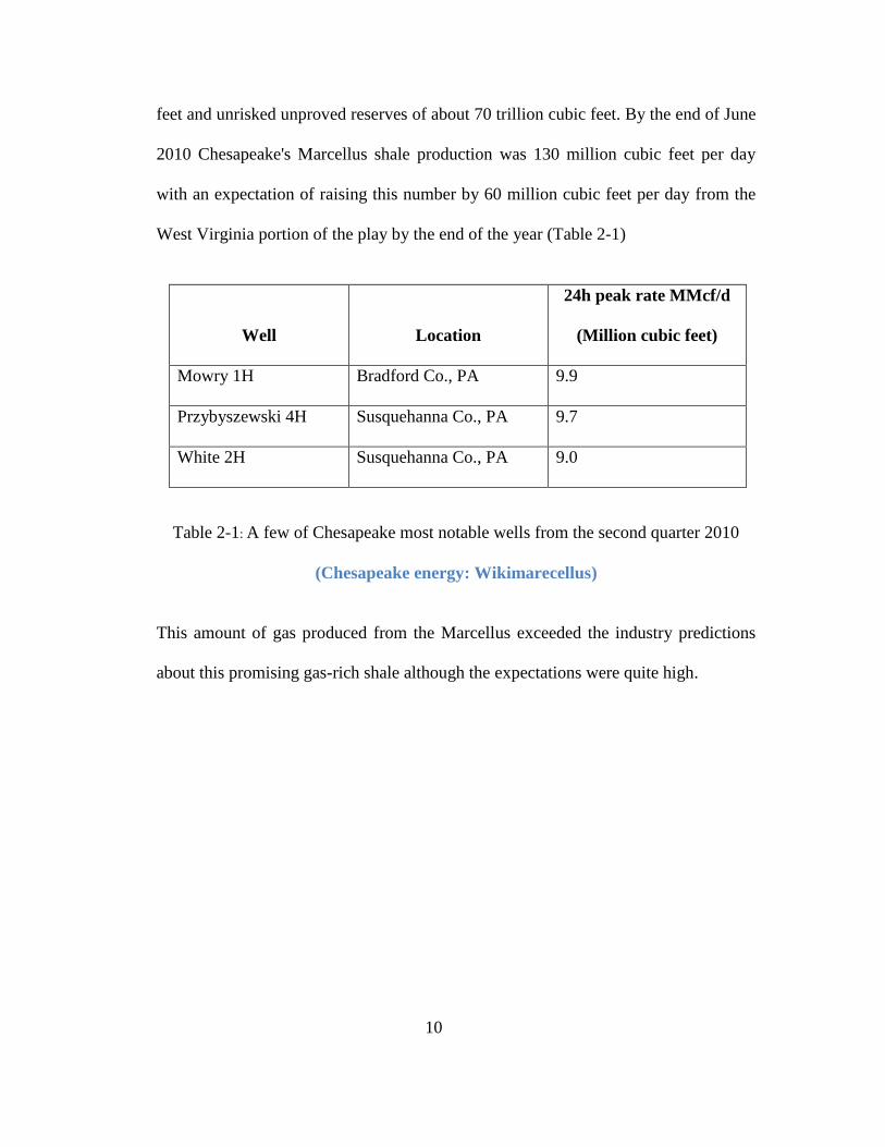
feet and unrisked unproved reserves of about 70 trillion cubic feet. By the end of June
2010 Chesapeake's Marcellus shale production was 130 million cubic feet per day
with an expectation of raising this number by 60 million cubic feet per day from the
West Virginia portion of the play by the end of the year (Table 2-1)
Well
Location
24h peak rate MMcf/d
(Million cubic feet)
Mowry 1H Bradford Co., PA 9.9
Przybyszewski 4H Susquehanna Co., PA 9.7
White 2H Susquehanna Co., PA 9.0
Table 2-1: A few of Chesapeake most notable wells from the second quarter 2010
(Chesapeake energy: Wikimarecellus)
This amount of gas produced from the Marcellus exceeded the industry predictions
about this promising gas-rich shale although the expectations were quite high.
11
Chapter 3 : Methodology
3.1 Seismic and well log data set
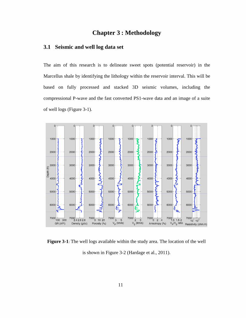
The aim of this research is to delineate sweet spots (potential reservoir) in the
Marcellus shale by identifying the lithology within the reservoir interval. This will be
based on fully processed and stacked 3D seismic volumes, including the
compressional P-wave and the fast converted PS1-wave data and an image of a suite
of well logs (Figure 3-1).
Figure 3-1: The well logs available within the study area. The location of the well
is shown in Figure 3-2 (Hardage et al., 2011).
12
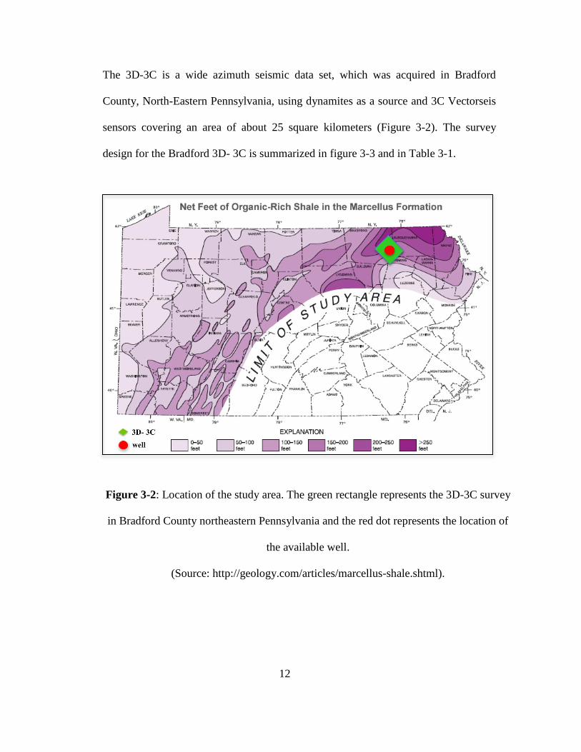
The 3D-3C is a wide azimuth seismic data set, which was acquired in Bradford
County, North-Eastern Pennsylvania, using dynamites as a source and 3C Vectorseis
sensors covering an area of about 25 square kilometers (Figure 3-2). The survey
design for the Bradford 3D- 3C is summarized in figure 3-3 and in Table 3-1.
Figure 3-2: Location of the study area. The green rectangle represents the 3D-3C survey
in Bradford County northeastern Pennsylvania and the red dot represents the location of
the available well.
(Source: http://geology.com/articles/marcellus-shale.shtml).
13
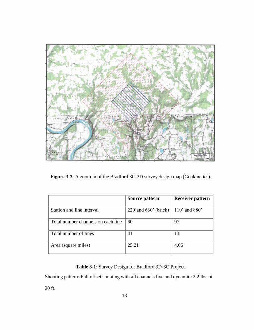
Figure 3-3: A zoom in of the Bradford 3C-3D survey design map (Geokinetics).
Source pattern Receiver pattern
Station and line interval 220’and 660’ (brick) 110’ and 880’
Total number channels on each line 60 97
Total number of lines 41 13
Area (square miles) 25.21 4.06
Table 3-1: Survey Design for Bradford 3D-3C Project.
Shooting pattern: Full offset shooting with all channels live and dynamite 2.2 lbs. at
20 ft.
14
3.2 Methodology
The occurrence of hydrocarbons in the Middle Devonian shale sequence is a result of
the coincidence of several factors including having relatively high amounts of organic
matter, suitable thermal maturity and naturally enhanced fracture porosity (Engelder
et al., 2009). The key for successful gas production is identifying shale with:
1. High TOC,
2. Maturation,
3. Can be easily stimulated (fracturable rock) to create pathways to the
wellbore.
The thermal maturity of the Marcellus is linked to its burial history. The Total
Organic Carbon information is deduced from its depositional setting as explained
previously. The same information can also be estimated from the well logs data,
especially from the gamma ray log. The brittleness, which is the focus of this
research, is proportional to Vp/Vs extracted from the 3D-3C seismic data set.
As the well logs available for this study are in PDF format, the first step was digitize
these well logs to transform them to an LAS file. The digitized well logs are then
loaded in Hampson-Russell software and used to generate the synthetic seismograms
for the PP (compressional) and the PS (converted) seismic sections. Once the
synthetic data are ready and with a high correlation coefficient (the highest, the best)
15
they can be loaded in Petrel. The seismic data corresponding to the compressional and
the fast converted waves are also loaded in Petrel.
Having the actual seismic data with the synthetic seismigrams is necessary to do the
tie between the well and the seismic easily. This tie will allow the seismic
interpretation of the needed horizons and in this study. The tie helps locating and
enables the interpretation of the top and the base of the Marcellus Formation in the PP
and in the PS seismic sections.
The difference between the top and the base of the obtained time structure maps is
calculated for the PP and for the PS to get the isochrons respectively (Tpp and Tps).
These isochrons are then combined to generate the Vp/Vs interval map.
It is possible to estimate the interval Vp/Vs from the traveltime of the horizons of
interest. Basically, based on the formula:
where,
=Velocity ratio estimated from PP- and PS-wave travel-time data,

16
ΔtPS = two-way travel time difference between two events in PS time, and
ΔtPP = two-way travel time difference between two events in PP time.
The Vp/Vs distribution map will help delineate different lithologies. Areas with low
Vp/Vs ratio indicate sandy zones and by consequence, high fracability.
Petrel could also generate different attributes, which help confirming the obtained
results about the brittleness. The coherency attribute for example could be generated
for the interpreted layers. This attribute enhance fault imaging highlighting subtle
faults that are overlooked on conventional seismic.
17
Chapter 4 : Results
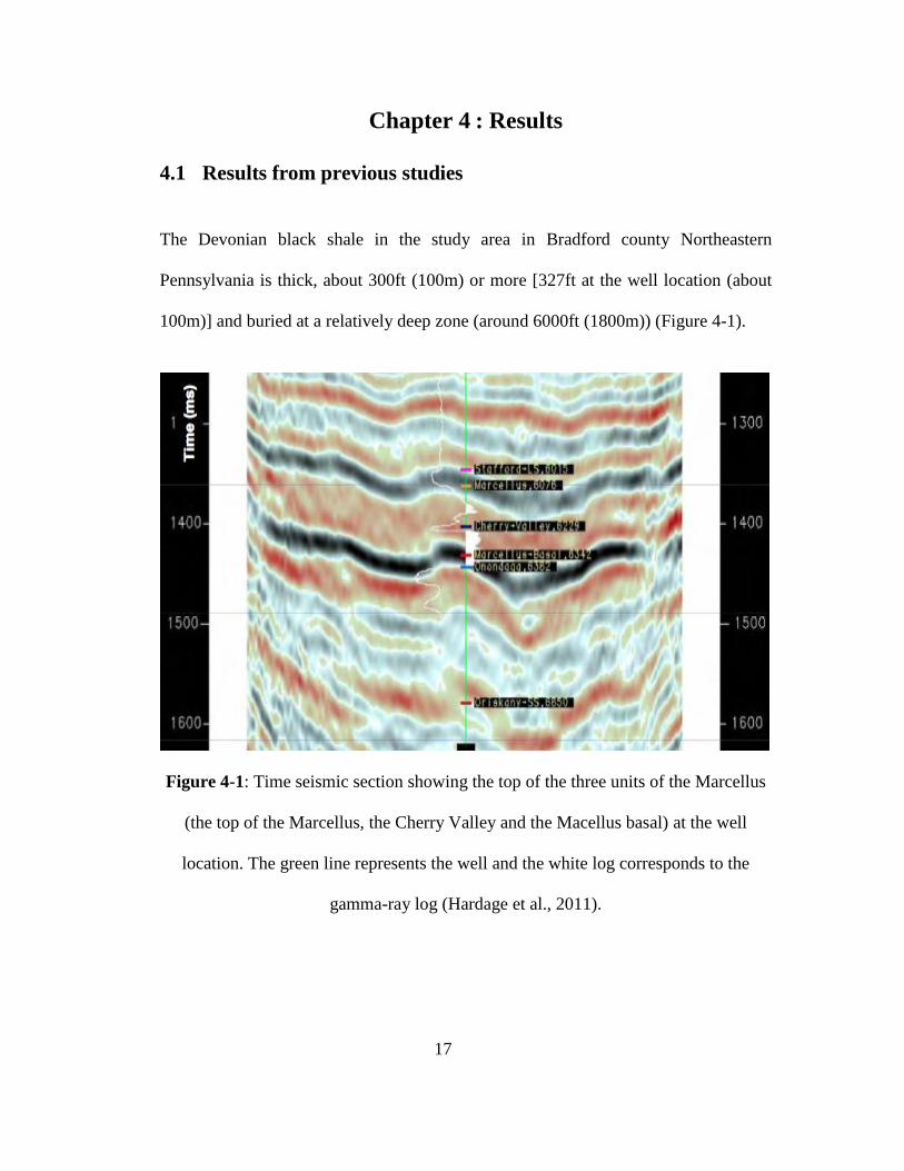
4.1 Results from previous studies
The Devonian black shale in the study area in Bradford county Northeastern
Pennsylvania is thick, about 300ft (100m) or more [327ft at the well location (about
100m)] and buried at a relatively deep zone (around 6000ft (1800m)) (Figure 4-1).
Figure 4-1: Time seismic section showing the top of the three units of the Marcellus
(the top of the Marcellus, the Cherry Valley and the Macellus basal) at the well
location. The green line represents the well and the white log corresponds to the
gamma-ray log (Hardage et al., 2011).
18
The burial thickness is related to the maturity. The greater the burial thickness is, the
higher the maturity is. The Marcellus burial history suggests that it was deposited at a
maximum water depth in an extreme anoxic condition which means a maximum
preservation of organic material and which leads to a high TOC.
It also affects permeability positively; the slight bioturbation helps preserving silt
laminae increasing lateral permeability.
4.2 Well log interpretation
The Marcellus Formation is subdivided into three units (Figure 4-1), the basal
Marcellus, the Cherry Valley member, and the upper Marcellus.
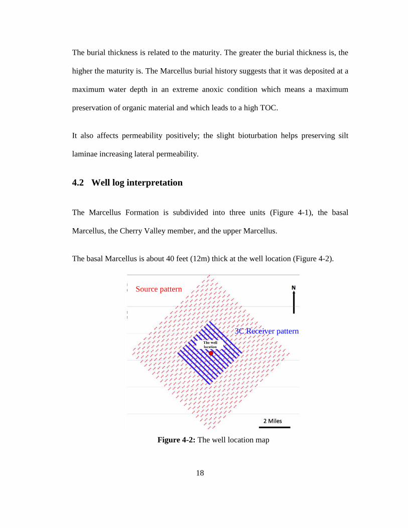
The basal Marcellus is about 40 feet (12m) thick at the well location (Figure 4-2).
Figure 4-2: The well location map
Source pattern
3C Receiver pattern
19
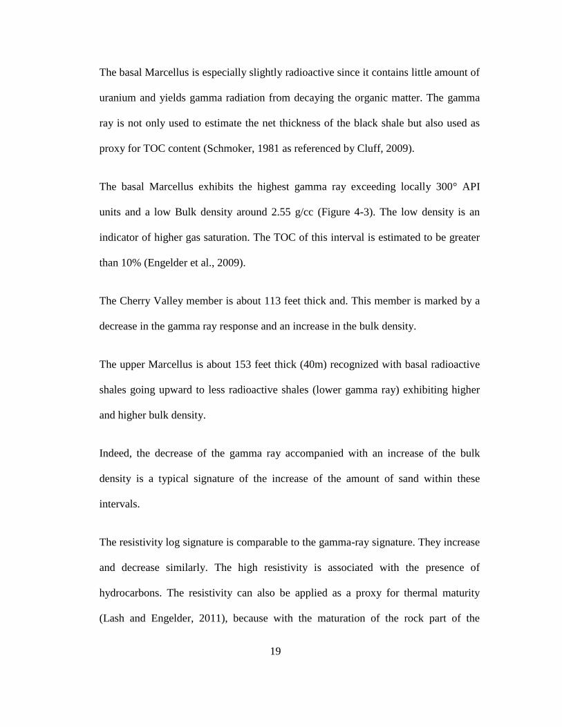
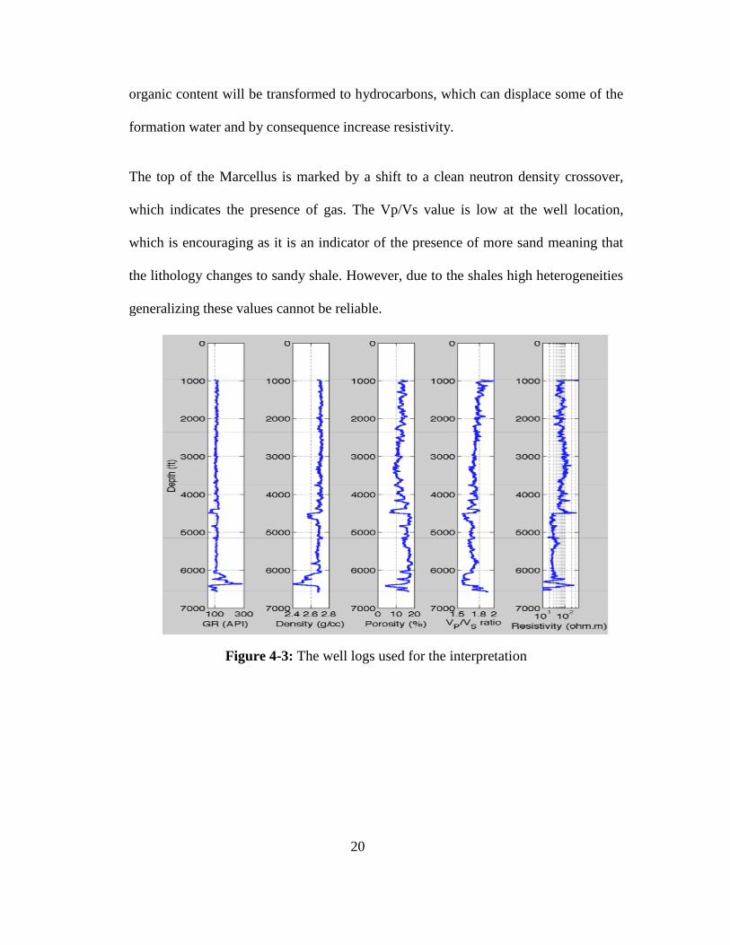
The basal Marcellus is especially slightly radioactive since it contains little amount of
uranium and yields gamma radiation from decaying the organic matter. The gamma
ray is not only used to estimate the net thickness of the black shale but also used as
proxy for TOC content (Schmoker, 1981 as referenced by Cluff, 2009).
The basal Marcellus exhibits the highest gamma ray exceeding locally 300° API
units and a low Bulk density around 2.55 g/cc (Figure 4-3). The low density is an
indicator of higher gas saturation. The TOC of this interval is estimated to be greater
than 10% (Engelder et al., 2009).
The Cherry Valley member is about 113 feet thick and. This member is marked by a
decrease in the gamma ray response and an increase in the bulk density.
The upper Marcellus is about 153 feet thick (40m) recognized with basal radioactive
shales going upward to less radioactive shales (lower gamma ray) exhibiting higher
and higher bulk density.
Indeed, the decrease of the gamma ray accompanied with an increase of the bulk
density is a typical signature of the increase of the amount of sand within these
intervals.
The resistivity log signature is comparable to the gamma-ray signature. They increase
and decrease similarly. The high resistivity is associated with the presence of
hydrocarbons. The resistivity can also be applied as a proxy for thermal maturity
(Lash and Engelder, 2011), because with the maturation of the rock part of the
20
organic content will be transformed to hydrocarbons, which can displace some of the
formation water and by consequence increase resistivity.
The top of the Marcellus is marked by a shift to a clean neutron density crossover,
which indicates the presence of gas. The Vp/Vs value is low at the well location,
which is encouraging as it is an indicator of the presence of more sand meaning that
the lithology changes to sandy shale. However, due to the shales high heterogeneities
generalizing these values cannot be reliable.
Figure 4-3: The well logs used for the interpretation
21
4.3 Brittleness Index
Shales can be classified as either ductile or brittle. The brittle shale fractures under
the effect of an applied stress while the ductile shale experience a certain plastic
behavior before being able to fracture. The brittleness and the ductility of the shales
are related to the ability of the rock to fracture and to propagate fracturations.
Mineralogical analysis is used to estimate the Brittleness Index. The mineralogy
affects the rigidity of the rock and by consequence impact the brittle or ductile
behavior. The amount of the quartz is responsible of the brittleness, which is a key
factor. The higher the amount of quartz is the better the shales can be easy to
stimulate. The more brittle the shale is, the more likely it is to yield high gas flow
rates (Jarvie et al., 2007).
Cores were collected at the well location to determine the mineralogy of the
Marcellus. The examination of the cores yielded to the information that the Marcellus
mineralogy is about 50% quartz, clay minerals 40% to 45% (Illite 3g/cc) and pyrite 5
to 10% (5g/cc) according to Hardage et al. (2011).
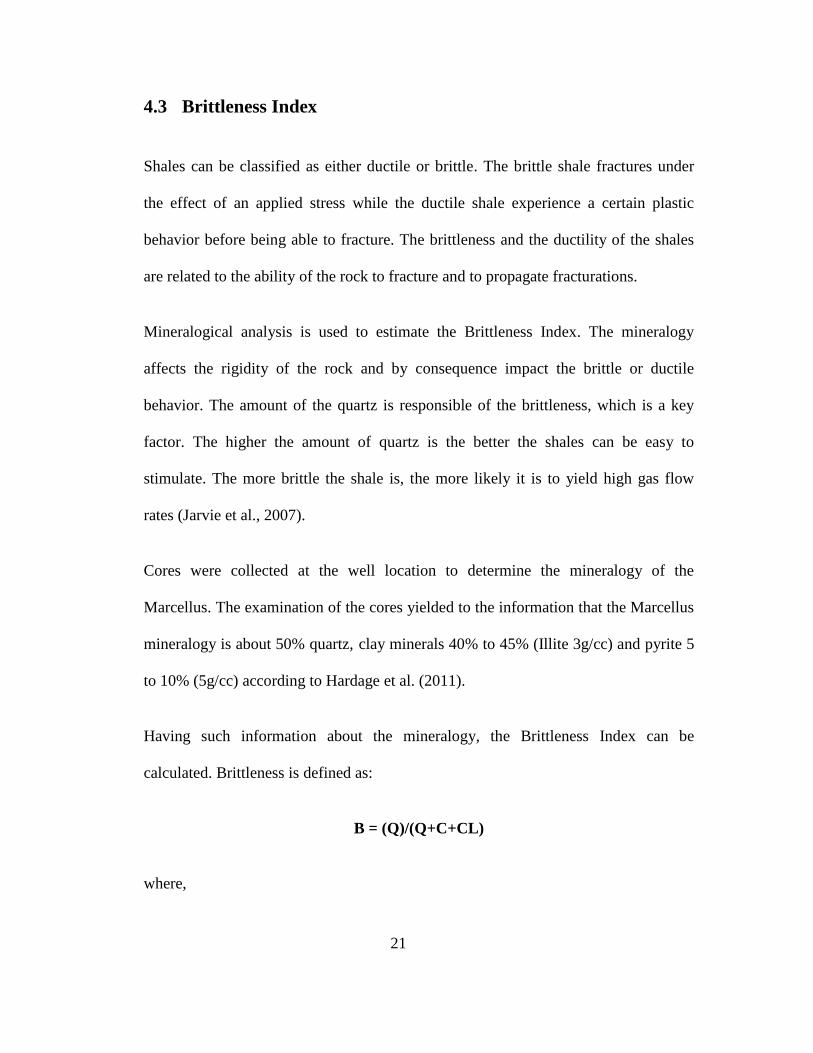
Having such information about the mineralogy, the Brittleness Index can be
calculated. Brittleness is defined as:
B = (Q)/(Q+C+CL)
where,
22
B – Brittleness,
Q – the amount of quartz,
C – the amount of carbonate,
Cl – the amount of clay.
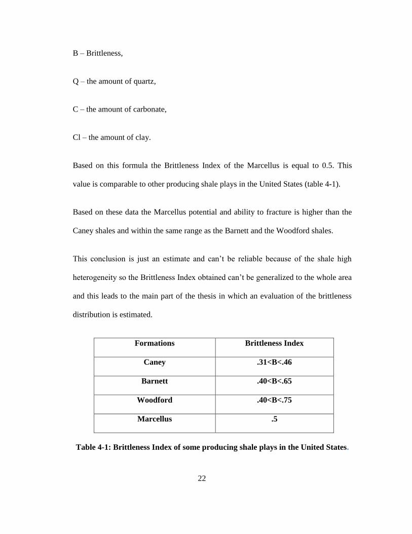
Based on this formula the Brittleness Index of the Marcellus is equal to 0.5. This
value is comparable to other producing shale plays in the United States (table 4-1).
Based on these data the Marcellus potential and ability to fracture is higher than the
Caney shales and within the same range as the Barnett and the Woodford shales.
This conclusion is just an estimate and can’t be reliable because of the shale high
heterogeneity so the Brittleness Index obtained can’t be generalized to the whole area
and this leads to the main part of the thesis in which an evaluation of the brittleness
distribution is estimated.
Formations Brittleness Index
Caney .31<B<.46
Barnett .40<B<.65
Woodford .40<B<.75
Marcellus .5
Table 4-1: Brittleness Index of some producing shale plays in the United States.
23
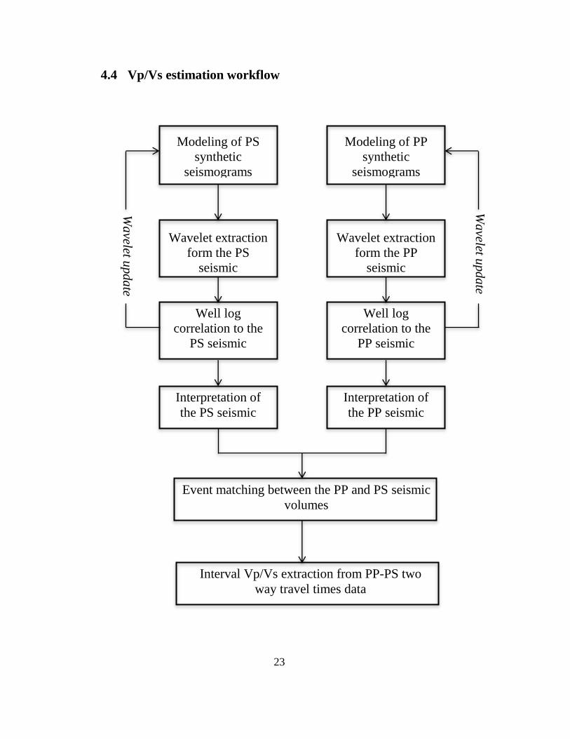
4.4 Vp/Vs estimation workflow
Modeling of PS
synthetic
seismograms
Modeling of PP
synthetic
seismograms
Wavelet extraction
form the PS
seismic
Wavelet extraction
form the PP
seismic
Well log
correlation to the
PS seismic
Well log
correlation to the
PP seismic
Interpretation of
the PS seismic
Interpretation of
the PP seismic
Event matching between the PP and PS seismic
volumes
Interval Vp/Vs extraction from PP-PS two
way travel times data
Wa
velet upda
te
Wa
velet upda
te
24
4.4.1 Synthetic seismograms modeling
Synthetic seismograms are generated always based on the velocity, the density, and
the seismic wavelet extracted from the well or from the seismic data available. The
seismic wavelet (as defined in Gukiyev, 2007) links the seismic data (traces) to the
geology (reflection coefficients). Generating the synthetic seismograms and
extracting the wavelet is based on the convolutional model, which consists on
convolving the reflectivity with a band-limited wavelet and adding random noise,
T=W*R+N
where,
T – seismic trace,
W – source wavelet,
R – reflection coefficient,
N – random noise.
The first stage to start with is the well tie process, which consists of the tie between
the well and the seismic data. The well tie procedure is done in three steps. The first
step is to model the synthetic seismograms, the second step is to extract the wavelet,
and the third step is to do the correlation.
25
The well tie purpose is to help locating the tops of the formations in the seismic data
allowing the seismic interpretation of the horizons of interest. It also generates the
depth to time curve, which is needed as the well logs data are in depth while the
seismic data are usually in time.
Generating the synthetic traces is an iterative process. The initial wavelet is a zero
phase wavelet with an amplitude spectrum derived from the available seismic data by
the Hampson - Russell software. This wavelet can either be extracted from the
seismic data or extracted from the traces neighboring the well.
The starting point is to compare the actual seismic data to the synthetic traces by
matching the same event in both traces and applying some stretching or squeezing in
order to enhance the shape of the wavelet (the only variable parameter); with every
new wavelet the synthetic is updated until obtaining the highest correlation
coefficient possible. The synthetic seismogram obtained corresponds to a zero-phase
synthetic seismogram, which is generated based on the ideal extracted wavelet.
Comparing the synthetic traces to the actual seismic data and doing the correlation
lead to the identification of the seismic horizons. Distinguishing the tops of the
formations and marking them on the seismic data allow the seismic interpretation of
the preferred horizons.
Strong amplitude events helped doing the correlation between the synthetic traces and
the seismic data.
26
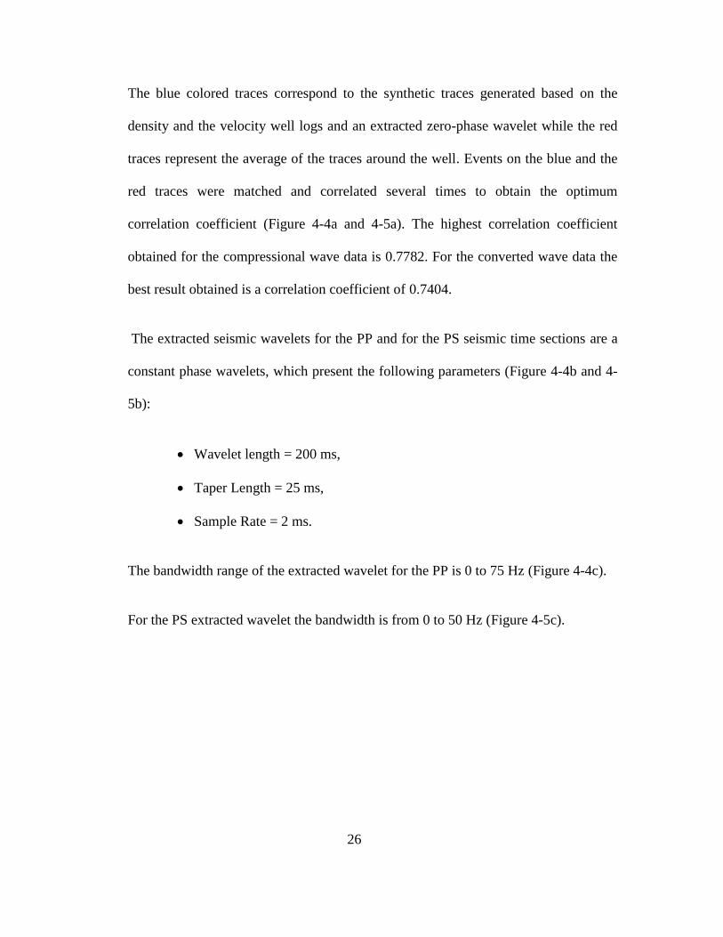
The blue colored traces correspond to the synthetic traces generated based on the
density and the velocity well logs and an extracted zero-phase wavelet while the red
traces represent the average of the traces around the well. Events on the blue and the
red traces were matched and correlated several times to obtain the optimum
correlation coefficient (Figure 4-4a and 4-5a). The highest correlation coefficient
obtained for the compressional wave data is 0.7782. For the converted wave data the
best result obtained is a correlation coefficient of 0.7404.
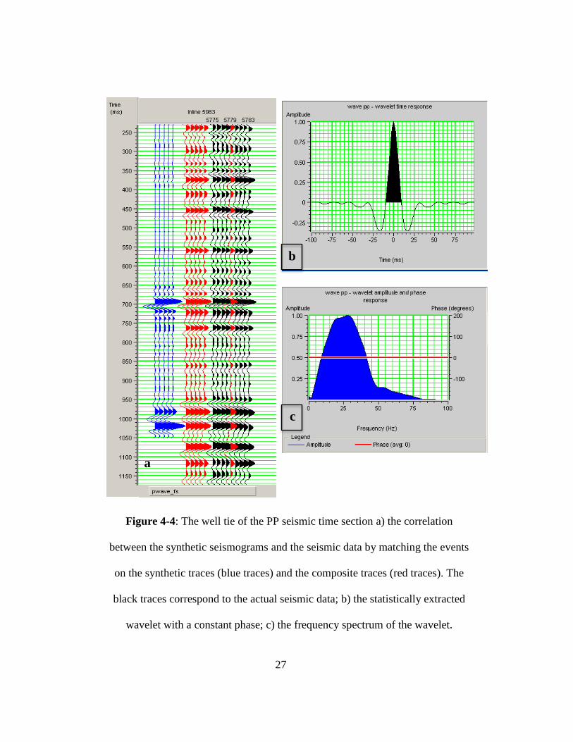
The extracted seismic wavelets for the PP and for the PS seismic time sections are a
constant phase wavelets, which present the following parameters (Figure 4-4b and 4-
5b):
Wavelet length = 200 ms,
Taper Length = 25 ms,
Sample Rate = 2 ms.
The bandwidth range of the extracted wavelet for the PP is 0 to 75 Hz (Figure 4-4c).
For the PS extracted wavelet the bandwidth is from 0 to 50 Hz (Figure 4-5c).
27
Figure 4-4: The well tie of the PP seismic time section a) the correlation
between the synthetic seismograms and the seismic data by matching the events
on the synthetic traces (blue traces) and the composite traces (red traces). The
black traces correspond to the actual seismic data; b) the statistically extracted
wavelet with a constant phase; c) the frequency spectrum of the wavelet.
a
b
c
28
Figure 4-5: The well tie of the PS seismic time section a) the correlation
between the synthetic seismograms and the seismic data by matching the
events on the synthetic traces (blue traces) and the composite traces (red
traces). The black traces correspond to the actual seismic data; b) the
statistically extracted wavelet with a constant phase; c) the frequency
spectrum of the wavelet.
a
b
c
29
4.4.2 PP and PS seismic interpretation
The top and the base of the Marcellus can be identified and located in the PP and the
PS seismic time sections based on the tie between the well and the seismic data.
Provided the synthetic seismograms generated previously, structural interpretation of
the top and the base of the Marcellus was achieved for both seismic time sections the
PP and the PS.
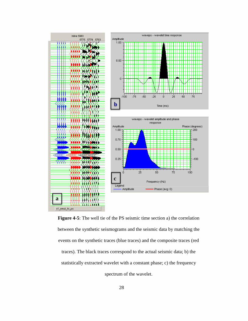
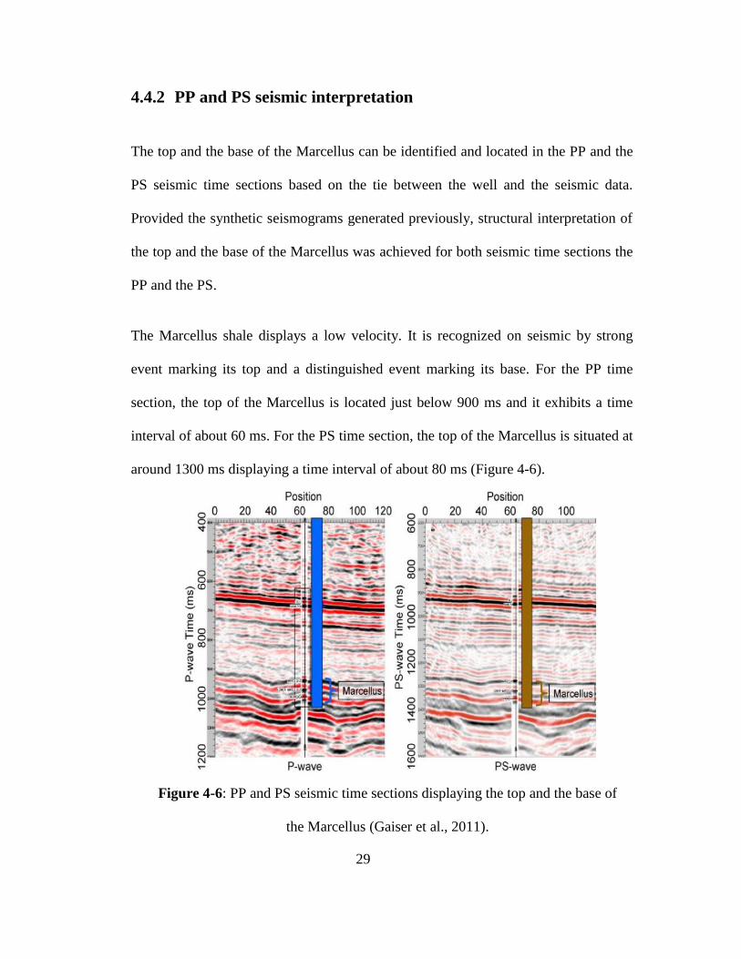
The Marcellus shale displays a low velocity. It is recognized on seismic by strong
event marking its top and a distinguished event marking its base. For the PP time
section, the top of the Marcellus is located just below 900 ms and it exhibits a time
interval of about 60 ms. For the PS time section, the top of the Marcellus is situated at
around 1300 ms displaying a time interval of about 80 ms (Figure 4-6).
Figure 4-6: PP and PS seismic time sections displaying the top and the base of
the Marcellus (Gaiser et al., 2011).
30
The reflectors marking the top and the base of the Marcellus were mainly horizontally
stratified. These reflectors were more coherent in the PS seismic time section
allowing better and easier interpretation. The PP time structure map share some
features with the PS time structure map, other features were revealed in either of both.
The reason why geological anomalies can be detected in the conventional P wave
section but not in the corresponding PS section or be seen in the PS section and goes
unseen in the corresponding PP, is that the shear waves and the compressional waves
respond in different manner for the same geological situation.
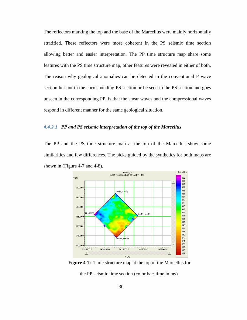
4.4.2.1 PP and PS seismic interpretation of the top of the Marcellus
The PP and the PS time structure map at the top of the Marcellus show some
similarities and few differences. The picks guided by the synthetics for both maps are
shown in (Figure 4-7 and 4-8).
Figure 4-7: Time structure map at the top of the Marcellus for
the PP seismic time section (color bar: time in ms).
31
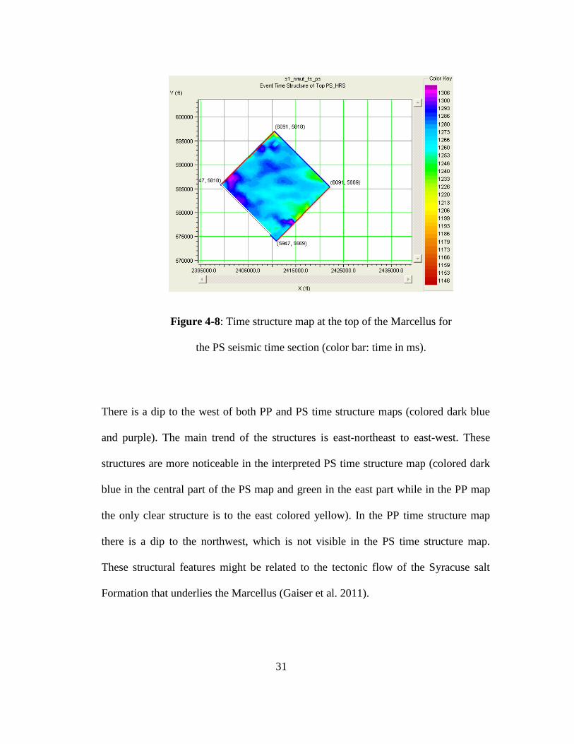
There is a dip to the west of both PP and PS time structure maps (colored dark blue
and purple). The main trend of the structures is east-northeast to east-west. These
structures are more noticeable in the interpreted PS time structure map (colored dark
blue in the central part of the PS map and green in the east part while in the PP map
the only clear structure is to the east colored yellow). In the PP time structure map
there is a dip to the northwest, which is not visible in the PS time structure map.
These structural features might be related to the tectonic flow of the Syracuse salt
Formation that underlies the Marcellus (Gaiser et al. 2011).
Figure 4-8: Time structure map at the top of the Marcellus for
the PS seismic time section (color bar: time in ms).
32
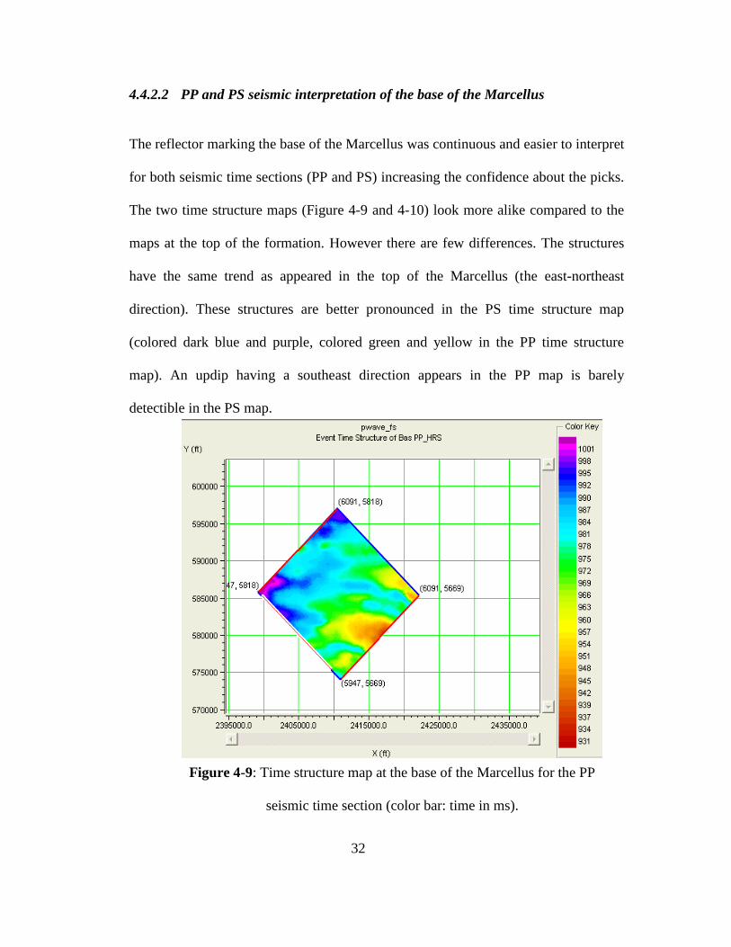
4.4.2.2 PP and PS seismic interpretation of the base of the Marcellus
The reflector marking the base of the Marcellus was continuous and easier to interpret
for both seismic time sections (PP and PS) increasing the confidence about the picks.
The two time structure maps (Figure 4-9 and 4-10) look more alike compared to the
maps at the top of the formation. However there are few differences. The structures
have the same trend as appeared in the top of the Marcellus (the east-northeast
direction). These structures are better pronounced in the PS time structure map
(colored dark blue and purple, colored green and yellow in the PP time structure
map). An updip having a southeast direction appears in the PP map is barely
detectible in the PS map.
Figure 4-9: Time structure map at the base of the Marcellus for the PP
seismic time section (color bar: time in ms).
33
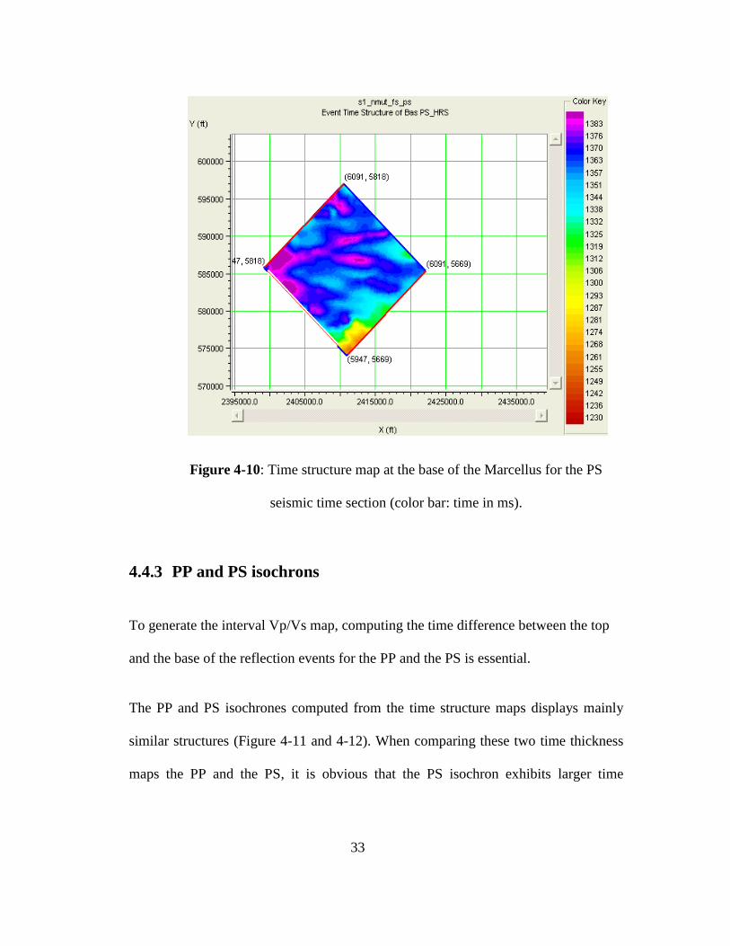
4.4.3 PP and PS isochrons
To generate the interval Vp/Vs map, computing the time difference between the top
and the base of the reflection events for the PP and the PS is essential.
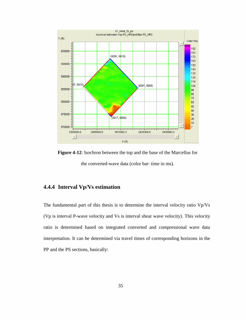
The PP and PS isochrones computed from the time structure maps displays mainly
similar structures (Figure 4-11 and 4-12). When comparing these two time thickness
maps the PP and the PS, it is obvious that the PS isochron exhibits larger time
Figure 4-10: Time structure map at the base of the Marcellus for the PS
seismic time section (color bar: time in ms).
34
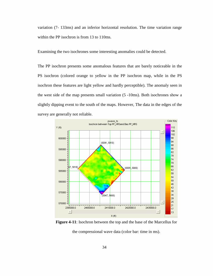
variation (7- 133ms) and an inferior horizontal resolution. The time variation range
within the PP isochron is from 13 to 110ms.
Examining the two isochrones some interesting anomalies could be detected.
The PP isochron presents some anomalous features that are barely noticeable in the
PS isochron (colored orange to yellow in the PP isochron map, while in the PS
isochron these features are light yellow and hardly perceptible). The anomaly seen in
the west side of the map presents small variation (5 -10ms). Both isochrones show a
slightly dipping event to the south of the maps. However, The data in the edges of the
survey are generally not reliable.
Figure 4-11: Isochron between the top and the base of the Marcellus for
the compressional wave data (color bar: time in ms).
35
4.4.4 Interval Vp/Vs estimation
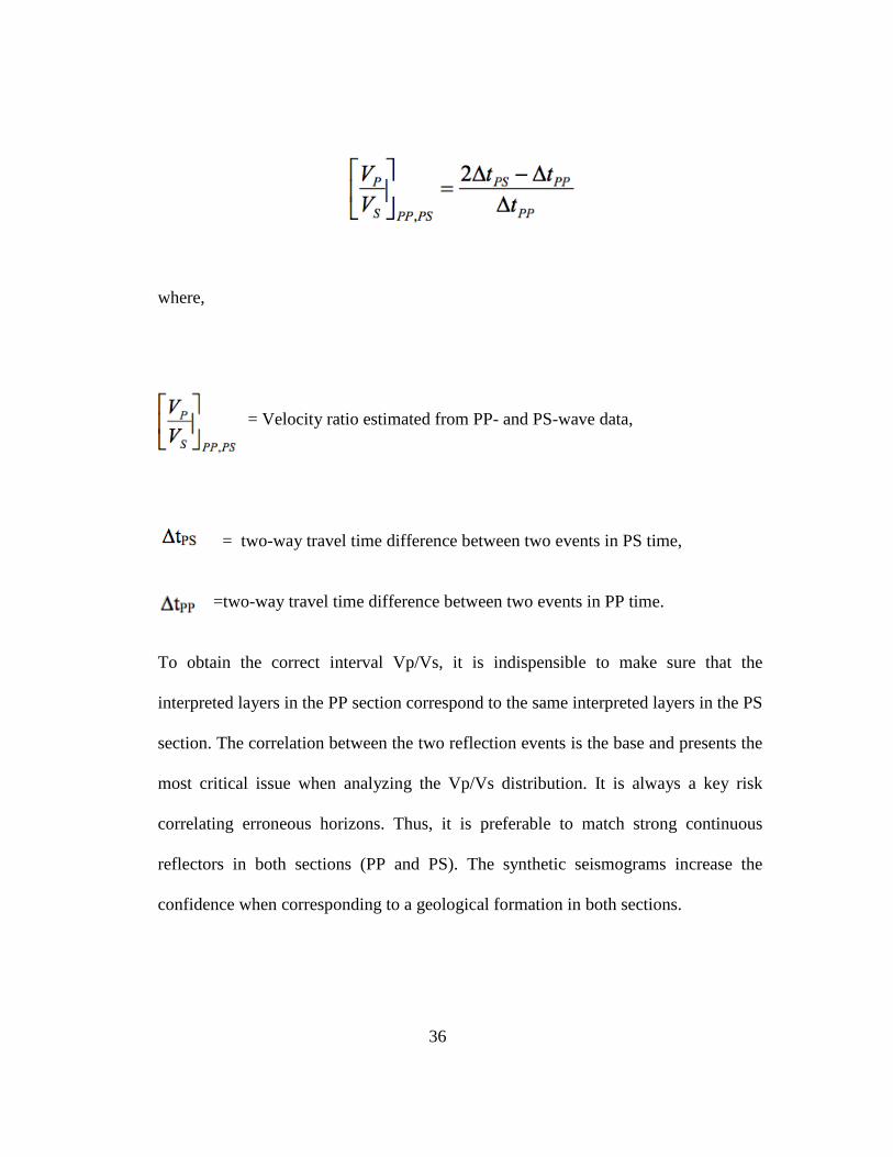
The fundamental part of this thesis is to determine the interval velocity ratio Vp/Vs
(Vp is interval P-wave velocity and Vs is interval shear wave velocity). This velocity
ratio is determined based on integrated converted and compressional wave data
interpretation. It can be determined via travel times of corresponding horizons in the
PP and the PS sections, basically:
Figure 4-12: Isochron between the top and the base of the Marcellus for
the converted-wave data (color bar: time in ms).
36
where,
= Velocity ratio estimated from PP- and PS-wave data,
= two-way travel time difference between two events in PS time,
=two-way travel time difference between two events in PP time.
To obtain the correct interval Vp/Vs, it is indispensible to make sure that the
interpreted layers in the PP section correspond to the same interpreted layers in the PS
section. The correlation between the two reflection events is the base and presents the
most critical issue when analyzing the Vp/Vs distribution. It is always a key risk
correlating erroneous horizons. Thus, it is preferable to match strong continuous
reflectors in both sections (PP and PS). The synthetic seismograms increase the
confidence when corresponding to a geological formation in both sections.
37
Ideally, this approach offers the opportunity to delineate prospects by mapping
lithological anomalies within the interval of interest. It can also be a tool for reservoir
characterization.
Vp/Vs can be an effective indicator of lithology, fractures, cracks and pore space
(Guliyev, 2007). It is also an indicator of pressure variation and pore fluid (Guliyev,
2007). In general, sandstones exhibit lower Vp/Vs values than shales. For sandstones,
it ranges from 1.5 to 1.7 and for shales it is around 2 (Guliyev, 2007). In addition, the
presence of gas within the formation lowers Vp/Vs. The Vp/Vs value also decreases
in overpressured areas (Guliyev, 2007). Another study conducted by Grigor (1998)
demonstrated empirically a proportional behavior of increasing anisotropy and
anellipticity with increasing Vp/Vs. Thus, a high Vp/Vs is an indicator of low
porosity as anisotropy increases with compaction (Guliyev, 2007). The increase of the
Vp/Vs can also be related to poorly consolidated or fractured zones.
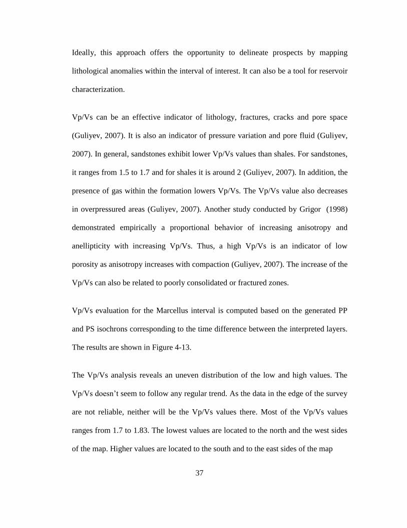
Vp/Vs evaluation for the Marcellus interval is computed based on the generated PP
and PS isochrons corresponding to the time difference between the interpreted layers.
The results are shown in Figure 4-13.
The Vp/Vs analysis reveals an uneven distribution of the low and high values. The
Vp/Vs doesn’t seem to follow any regular trend. As the data in the edge of the survey
are not reliable, neither will be the Vp/Vs values there. Most of the Vp/Vs values
ranges from 1.7 to 1.83. The lowest values are located to the north and the west sides
of the map. Higher values are located to the south and to the east sides of the map
38
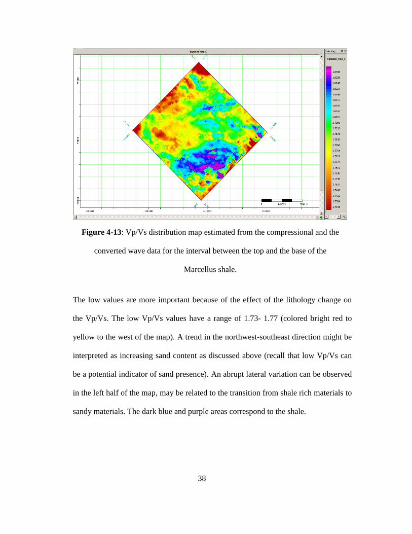
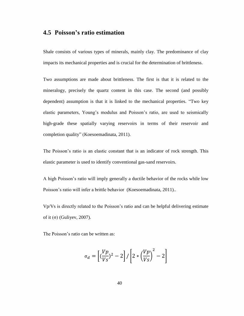
The low values are more important because of the effect of the lithology change on
the Vp/Vs. The low Vp/Vs values have a range of 1.73- 1.77 (colored bright red to
yellow to the west of the map). A trend in the northwest-southeast direction might be
interpreted as increasing sand content as discussed above (recall that low Vp/Vs can
be a potential indicator of sand presence). An abrupt lateral variation can be observed
in the left half of the map, may be related to the transition from shale rich materials to
sandy materials. The dark blue and purple areas correspond to the shale.
Figure 4-13: Vp/Vs distribution map estimated from the compressional and the
converted wave data for the interval between the top and the base of the
Marcellus shale.
39
This lateral variation may be due to the shales heterogeneity and could be detected
using the Vp/Vs attribute because the geological anomaly is either present in the
compressional wave section or in the converted wave section.
There is a fairly high concentration of anomalies (low Vp/Vs values, yellow spots) all
over the map and especially to the east (the right half) that could be inferred as sand
bodies.
The lateral distribution of the Vp/Vs allows delineating potential prospects. These
prospects are correlated with a middle range of time thickness for the PP and for the
PS (about 55ms for the PP and about 65ms for the PS) and a low Vp/Vs
corresponding approximately to 1.75.
Thus, the Vp/Vs extracted from traveltimes and then from the seismic can be
correlated with the lithology as the presence of sandier materials lowers the Vp/Vs.
The Vp/Vs attribute is applied to identify production targets. However, care must be
taken when applying this method. For instance, it can’t be conducted when having a
thin interval because there will not be a corresponding reflection events at the
boundaries (Guliyev, 2007). Also, to spot an anomaly within the interval Vp/Vs map,
this anomaly must be detected within at least one of the seismic sections (Guliyev,
2007). In addition, the Vp/Vs can be useful when distinguishing between two
different lithologies (shale and sand) but might not be as reliable when determining
subtle lithological change within one lithology (Hendrick, 2005). Careful evaluation
of the Vp/Vs is required to avoid any misinterpretation or over interpretation.
40
4.5 Poisson’s ratio estimation
Shale consists of various types of minerals, mainly clay. The predominance of clay
impacts its mechanical properties and is crucial for the determination of brittleness.
Two assumptions are made about brittleness. The first is that it is related to the
mineralogy, precisely the quartz content in this case. The second (and possibly
dependent) assumption is that it is linked to the mechanical properties. “Two key
elastic parameters, Young’s modulus and Poisson’s ratio, are used to seismically
high-grade these spatially varying reservoirs in terms of their reservoir and
completion quality” (Koesoemadinata, 2011).
The Poisson’s ratio is an elastic constant that is an indicator of rock strength. This
elastic parameter is used to identify conventional gas-sand reservoirs.
A high Poisson’s ratio will imply generally a ductile behavior of the rocks while low
Poisson’s ratio will infer a brittle behavior (Koesoemadinata, 2011)..
Vp/Vs is directly related to the Poisson’s ratio and can be helpful delivering estimate
of it (σ) (Guliyev, 2007).
The Poisson’s ratio can be written as:
[
] [ (
)
]
41
where,
is the dynamic Poisson’s ratio;
Vp/Vs is the velocity ratio.
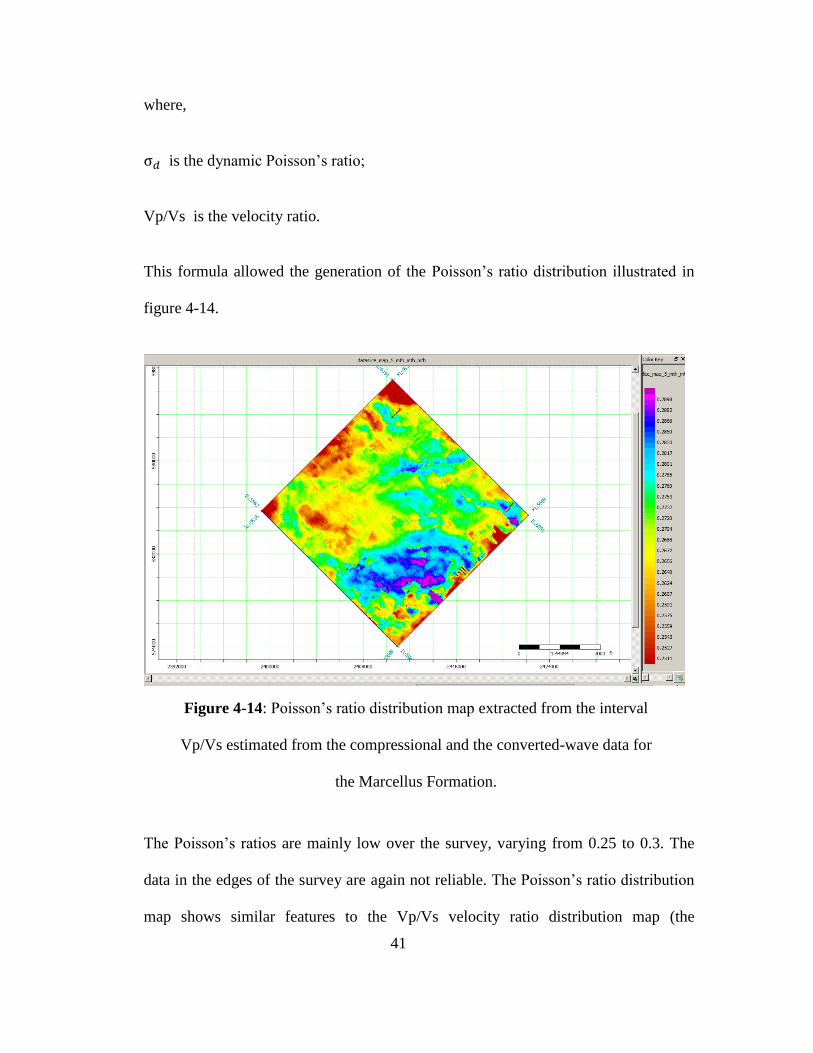
This formula allowed the generation of the Poisson’s ratio distribution illustrated in
figure 4-14.
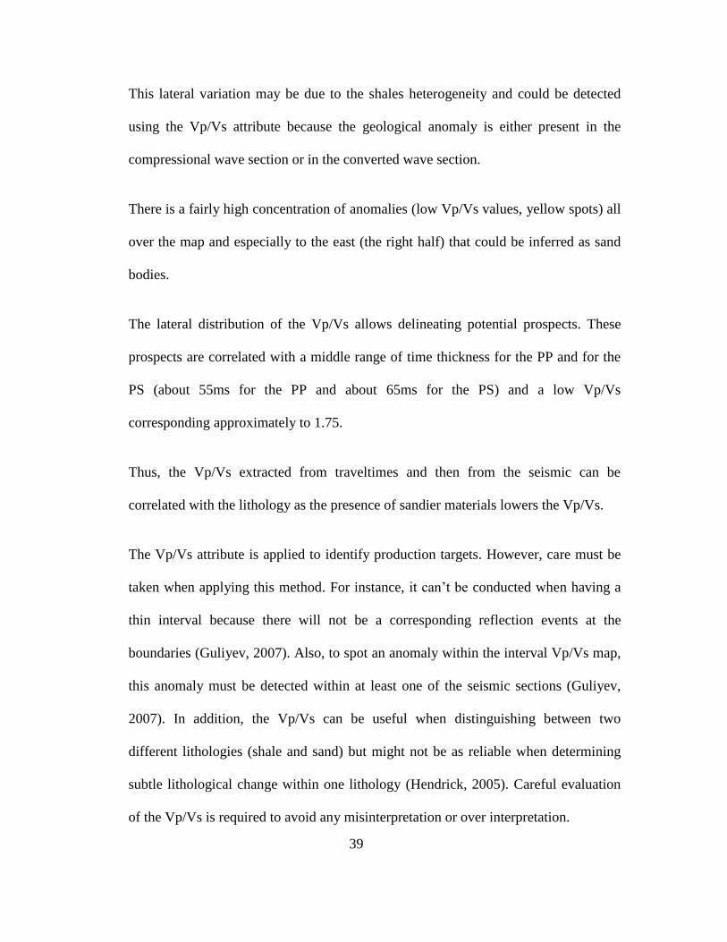
The Poisson’s ratios are mainly low over the survey, varying from 0.25 to 0.3. The
data in the edges of the survey are again not reliable. The Poisson’s ratio distribution
map shows similar features to the Vp/Vs velocity ratio distribution map (the
Figure 4-14: Poisson’s ratio distribution map extracted from the interval
Vp/Vs estimated from the compressional and the converted-wave data for
the Marcellus Formation.

42
Poisson’s ratio and the Vp/Vs are directly related). The low values are mainly located
to the west side of the map (left half) colored bright red. There are some anomalous
low values allover the map matching the low Vp/Vs spots. The high values are
colored dark blue to purple and located to the west of the map confirming the results
obtained in the Vp/Vs velocity ratio map. The area of the anomaly is the same in the
Poisson’s ratio map and the area corresponding to the shale in the west of the map
looks narrowed down.
The Poisson’s ratio map is a transformation of the Vp/Vs map and similarly can help
in delineating potential prospects.
43
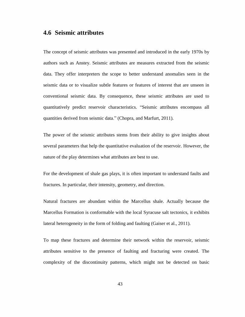
4.6 Seismic attributes
The concept of seismic attributes was presented and introduced in the early 1970s by
authors such as Anstey. Seismic attributes are measures extracted from the seismic
data. They offer interpreters the scope to better understand anomalies seen in the
seismic data or to visualize subtle features or features of interest that are unseen in
conventional seismic data. By consequence, these seismic attributes are used to
quantitatively predict reservoir characteristics. “Seismic attributes encompass all
quantities derived from seismic data.” (Chopra, and Marfurt, 2011).
The power of the seismic attributes stems from their ability to give insights about
several parameters that help the quantitative evaluation of the reservoir. However, the
nature of the play determines what attributes are best to use.
For the development of shale gas plays, it is often important to understand faults and
fractures. In particular, their intensity, geometry, and direction.
Natural fractures are abundant within the Marcellus shale. Actually because the
Marcellus Formation is conformable with the local Syracuse salt tectonics, it exhibits
lateral heterogeneity in the form of folding and faulting (Gaiser et al., 2011).
To map these fractures and determine their network within the reservoir, seismic
attributes sensitive to the presence of faulting and fracturing were created. The
complexity of the discontinuity patterns, which might not be detected on basic
44
seismic might be enhanced. To highlight discontinuities within seismic data several
attributes could be used.
The most common attributes used to detect these discontinuities are the coherence
attribute (the variance) and the curvature attribute. These attributes are primarily used
to enhance subtle faults and discontinuities that are less obvious on conventional
seismic data. Petrel software was used to generate the coherency and curvature
attribute for the interpreted PP and PS.
4.6.1 Coherency attribute
The coherency attribute was developed in the middle of the 1990s. It highlights
discontinuities registered within the seismic data and interpreted as faults
(Rummerfeld et al., 1954 and Lindseth, 2005). The coherency attribute measures the
lateral changes between the seismic waveforms and the amplitude. Coherent
waveforms indicate a horizontally stratified continuous layer whereas the abrupt
change of the waveforms reflects the presence of discontinuities generally faults and
fracture.
Several attributes are available which are capable of highlighting fault features.
Variance is an excellent starting point to capture fault expression in the data.
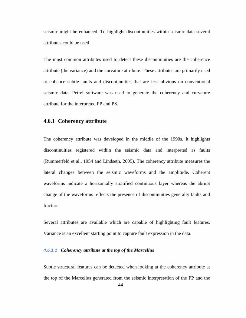
4.6.1.1 Coherency attribute at the top of the Marcellus
Subtle structural features can be detected when looking at the coherency attribute at
the top of the Marcellus generated from the seismic interpretation of the PP and the
45
PS seismic sections (Figure 4-15 and 4-16). The white color in the maps indicates a
continuous reflector while the black red and yellow are indicators of more and more
variance.
Figure 4-15: Coherency attribute at the top of the Marcellus
corresponding to the PP interpreted section.
Figure 4-16: Coherency attribute at the top of the Marcellus
corresponding to the PS interpreted section.
46
The coherency map corresponding to the PS interpreted section displays more
incoherency and by consequence major faults are better seen within it. The faults and
fractures exhibit mainly the east-northeast direction. Other smaller discontinuities
display a northwest-southeast direction. This information is conformant with the
literature about the two fractures set within the Marcellus the J1 and the J2.
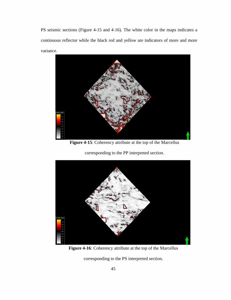
4.6.1.2 Coherency attribute at the base of the Marcellus
The coherency attributes corresponding to the interpreted PP and PS sections at the
base of the Marcellus are illustrated in Figure 4-17 and 4-18.
Figure 4-17: Coherency attribute at the base of the Marcellus
corresponding to the PP interpreted section.

47
For the top of the Marcellus, the coherency attributes in the PP and the PS showed
almost the same structural features clearer in the PS section. However, for the base of
the Marcellus, the two maps are complementary. Some faults are better seen within
the PP section, the others are more developed within the PS section. The basal
Marcellus looks more coherent compared to the top and the PP section appears more
coherent than the PS section. The data in the edges are in general inconsistent.
4.6.2 Curvature attribute
The curvature attribute is a second-derivative calculation of time or depth structure.
Figure 4-18: Coherency attribute at the base of the Marcellus
corresponding to the PS interpreted section.
48
The curvature attribute has been used for years not only to delineate subtle and small-
scale faults but also to map flexures and folds related to fracturing. It can help detect
fractures distribution regardless of their direction. Curvature and coherence attributes
are currently the most effective attributes when trying to predict fractures in post-
stack data (Chopra et al., 2011).
Curvature will be a zero when displaying a continuous straight line and the more the
curve is bent the larger the curvature will be.
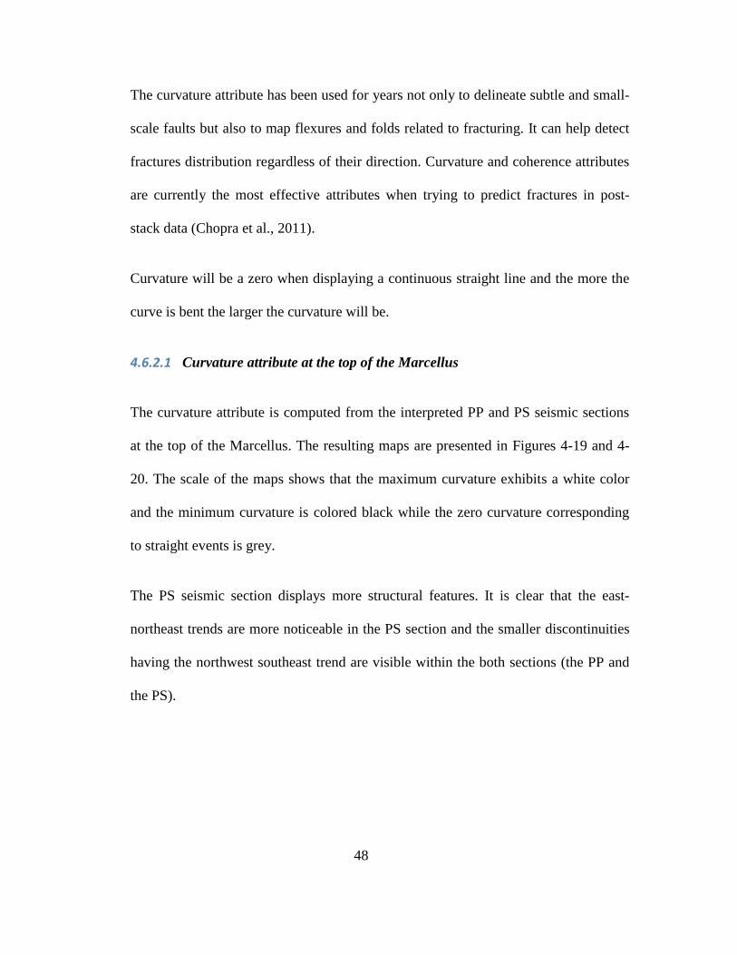
4.6.2.1 Curvature attribute at the top of the Marcellus
The curvature attribute is computed from the interpreted PP and PS seismic sections
at the top of the Marcellus. The resulting maps are presented in Figures 4-19 and 4-
20. The scale of the maps shows that the maximum curvature exhibits a white color
and the minimum curvature is colored black while the zero curvature corresponding
to straight events is grey.
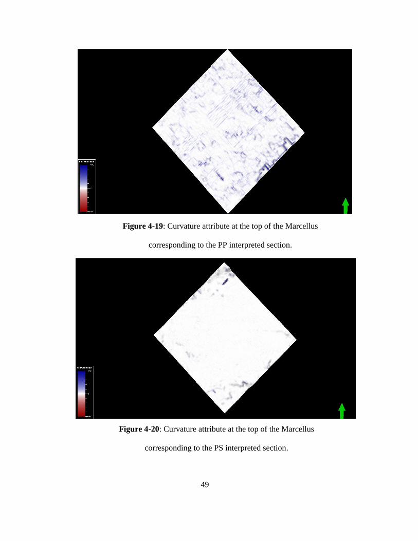
The PS seismic section displays more structural features. It is clear that the east-
northeast trends are more noticeable in the PS section and the smaller discontinuities
having the northwest southeast trend are visible within the both sections (the PP and
the PS).
49
Figure 4-19: Curvature attribute at the top of the Marcellus
corresponding to the PP interpreted section.
Figure 4-20: Curvature attribute at the top of the Marcellus
corresponding to the PS interpreted section.
50
The areas corresponding to the maximum curvature within the two maps are well
correlated with the areas exhibiting low coherency within the variance map.
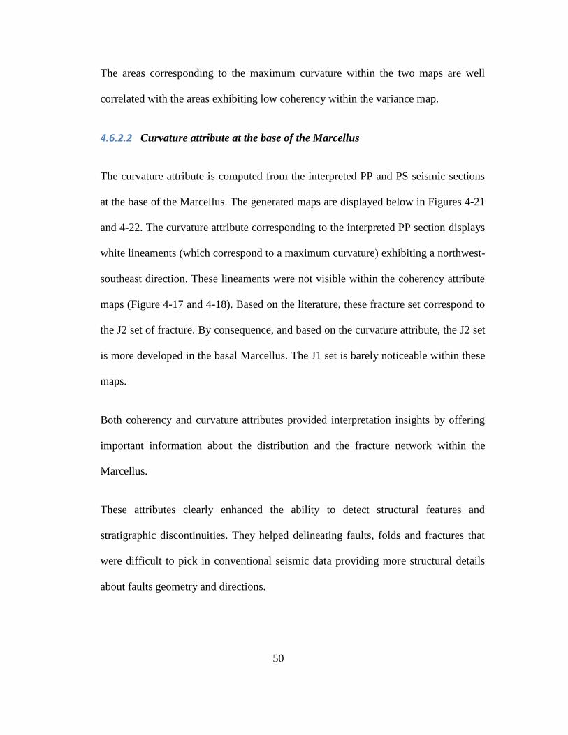
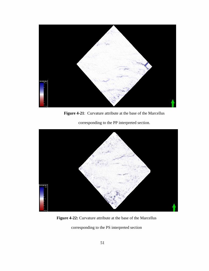
4.6.2.2 Curvature attribute at the base of the Marcellus
The curvature attribute is computed from the interpreted PP and PS seismic sections
at the base of the Marcellus. The generated maps are displayed below in Figures 4-21
and 4-22. The curvature attribute corresponding to the interpreted PP section displays
white lineaments (which correspond to a maximum curvature) exhibiting a northwest-
southeast direction. These lineaments were not visible within the coherency attribute
maps (Figure 4-17 and 4-18). Based on the literature, these fracture set correspond to
the J2 set of fracture. By consequence, and based on the curvature attribute, the J2 set
is more developed in the basal Marcellus. The J1 set is barely noticeable within these
maps.
Both coherency and curvature attributes provided interpretation insights by offering
important information about the distribution and the fracture network within the
Marcellus.
These attributes clearly enhanced the ability to detect structural features and
stratigraphic discontinuities. They helped delineating faults, folds and fractures that
were difficult to pick in conventional seismic data providing more structural details
about faults geometry and directions.
51
Figure 4-21: Curvature attribute at the base of the Marcellus
corresponding to the PP interpreted section.
Figure 4-22: Curvature attribute at the base of the Marcellus
corresponding to the PS interpreted section

52
These attributes strongly suggest the abundance of fractures within the Marcellus.
The maps indicate the high density of fracturing within the survey. However, these
fractures need to be unhealed to allow the gas to flow otherwise if the fractures are
closed (mineralized) they will act as a permeability barrier prohibiting the gas from
flowing to the wellbore.
53
4.7 Fold map calculations
When doing the seismic interpretation of the compressional and the converted-wave
data shown in the previous section, it was noticeable that the seismic data was of a
high quality within the central part of the survey. However, the quality of the seismic
data degrades as it gets farther from the center. This makes the interpretation difficult
at the edges and which in turn affects the reliability of the results obtained, not only
for the time structure maps but also for the isochrons, the Vp/Vs map, the Poisson’s
ratio map as well as for the curvature and the coherency attributes maps.
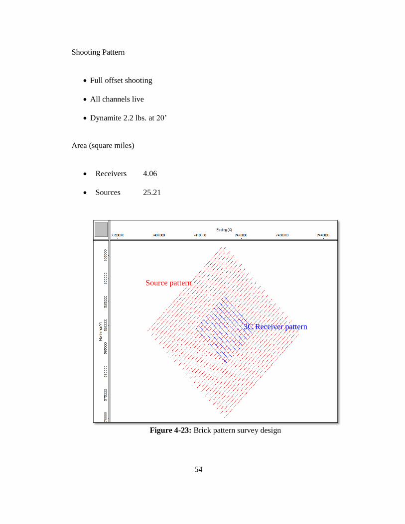
For a better understanding of the seismic data quality variation distribution, bin fold,
distribution of offset and azimuth and rose diagram was computed using Omni 3D
seismic survey design package. The survey was acquired using a brick pattern (Figure
4-23).
Source Pattern:
Station and line interval: 220’ and 660’ (brick);
Total number of channels on each line =60;
Total number of lines: 41
Receiver Pattern
Station and line interval: 110’ & 880’
Total number of channels on each line =97
Total number of lines: 13
54
Shooting Pattern
Full offset shooting
All channels live
Dynamite 2.2 lbs. at 20’
Area (square miles)
Receivers 4.06
Sources 25.21
Figure 4-23: Brick pattern survey design
Source pattern
3C Receiver pattern
55
The bin fold map is usually computed before shooting a seismic survey and after
selecting its design to obtain the optimum fold. Usually, the signal/noise can only be a
certain amount enhanced once the design and the fold is are finished.
The fold is defined according to Cordsen (1995) as “the number of midpoints which
are stacked within a CMP bin”. In the PS case, this would be the number of converted
The fold is variable. Different bins exhibit different folds due to the offset and
azimuth variability. It also varies with depth, as with increasing offset distance the
stack will include deeper reflectors.
Theoretically, to increase the fold the size of the bin needs to be doubled considering
that the midpoints coincide with the middle of the bins.
Several ways are used to calculate the fold. The basic equation is:
Fold = NS * NC * (Cordsen, 1995)
where,
NS= the number of source points per unit area;
NC is the number of channels; and
b is the bin dimension.
Considering the assumption that the bins are squares (Cordsen, 1995),
56
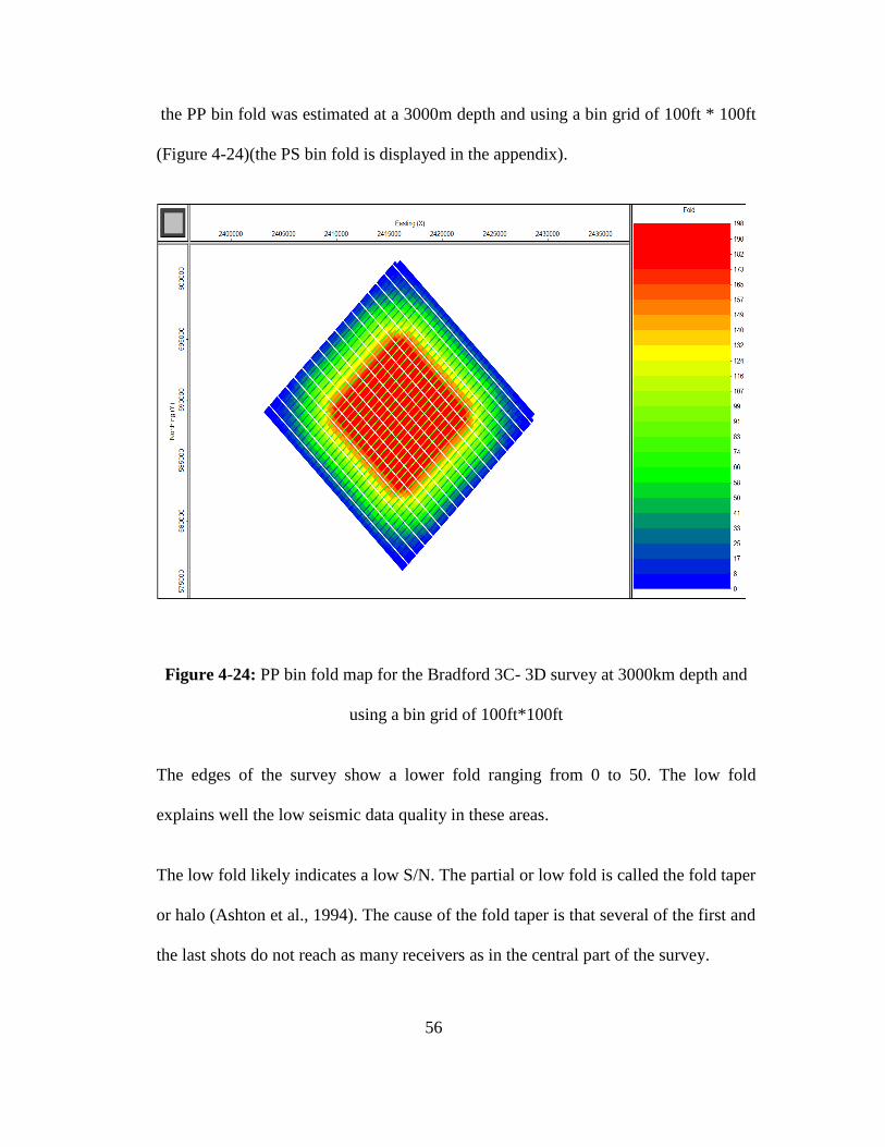
the PP bin fold was estimated at a 3000m depth and using a bin grid of 100ft * 100ft
(Figure 4-24)(the PS bin fold is displayed in the appendix).
Figure 4-24: PP bin fold map for the Bradford 3C- 3D survey at 3000km depth and
using a bin grid of 100ft*100ft
The edges of the survey show a lower fold ranging from 0 to 50. The low fold
explains well the low seismic data quality in these areas.
The low fold likely indicates a low S/N. The partial or low fold is called the fold taper
or halo (Ashton et al., 1994). The cause of the fold taper is that several of the first and
the last shots do not reach as many receivers as in the central part of the survey.
57
The values of the fold increase toward the center of the survey reaching about 198.
The high fold correlates with the high seismic data quality as expected.
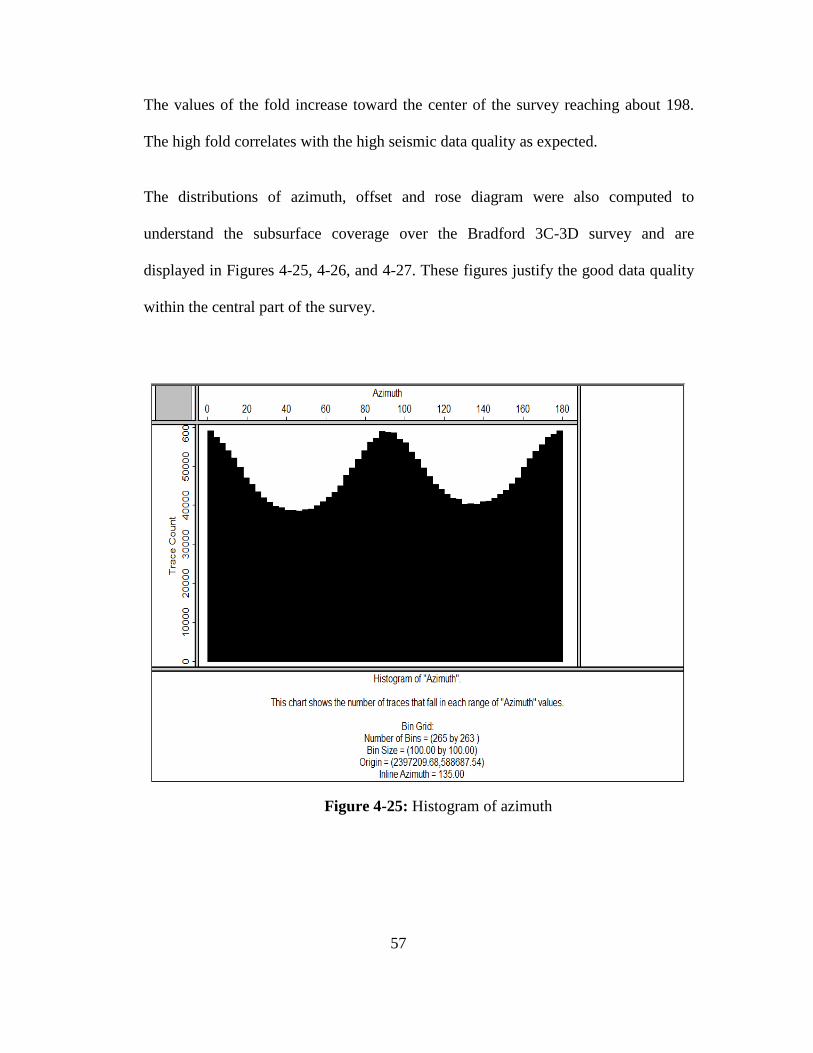
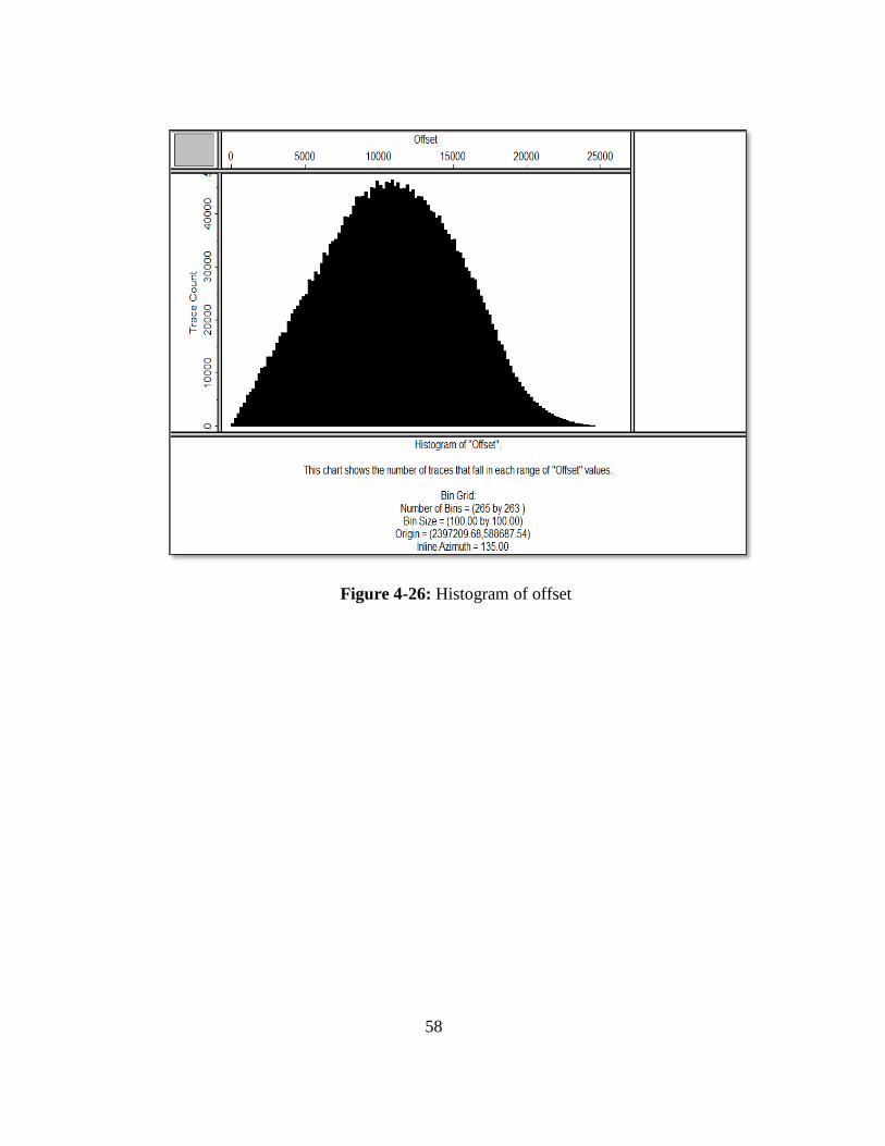
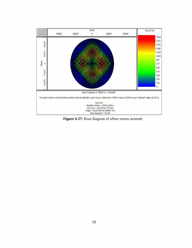
The distributions of azimuth, offset and rose diagram were also computed to
understand the subsurface coverage over the Bradford 3C-3D survey and are
displayed in Figures 4-25, 4-26, and 4-27. These figures justify the good data quality
within the central part of the survey.
Figure 4-25: Histogram of azimuth
58
Figure 4-26: Histogram of offset
59
Figure 4-27: Rose diagram of offset versus azimuth
60
4.8 Post–stack seismic inversion
The main objective of applying a post-stack seismic inversion is to convert the
seismic data to more closely represent the properties of the geologic layers. The
inversion consists of extracting the possible geologies that cause the seismic
reflections.
Inversion usually first derives impedance changes from seismic data as seismic
amplitude shows the boundaries between rock layers, which is a property useful for
geological interpretation.
The inversion is getting the geology from the seismic (the forward modeling:
extracting the seismic from the geology).
Acoustic impedance units can be any combination of P-wave and density units.
The difference in acoustic impedance between rock layers determines the reflection
coefficient.
Then the source wavelet is convolved with the earth reflectivity plus the noise to
produce the seismic trace.
The effect of convolving the wavelet with the reflectivity is to remove much of the
high- frequency detail.
In simple post-stack inversion (example: in the Strata inversion package):
61
There are no multiples modeled;
Transmission loss and geometric spreading are ignored;
Frequency-dependent absorption is ignored;
The wavelet may be time varying (Strata workshop).
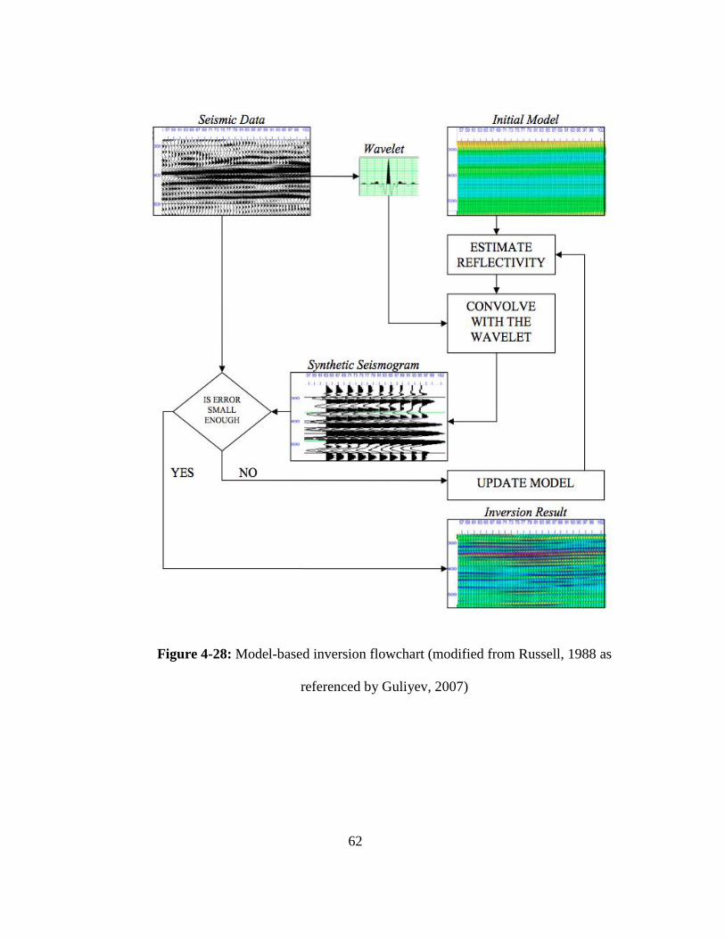
The inversion process is summarized in Figure 4-28. Theoretically, the inversion
attempts to recover the lost frequencies. Seismic data usually does not contain the low
frequencies needed for to recover absolute impedances through inversion. These can
be provided by well logs, which record both lower and higher frequency data than
seismic (Guliyev, 2007).
Early inversions were limited to post-stack data, and did not properly take into
account wavelet interference.
Later developments incorporated the extracted wavelet, and, combined with pre-stack
AVO analysis, produced numerical results consistent with well log measurements.
Current inversion technology has shifted attention to the quality of the input seismic
data, and the model building.
62
Figure 4-28: Model-based inversion flowchart (modified from Russell, 1988 as
referenced by Guliyev, 2007)
63
The use of inversion has been developing and one of its current uses is to predict
lithological parameters such as porosity and water saturation.
There are many inversion algorithms. These inversion techniques share a common
problem: the non-uniqueness.
There is more than one possible geological model consistent with the seismic data.
The only way to decide between the possibilities is to use other information, not
present in the seismic data.
These other information is often provided in several ways:
An initial model;
Constraints on how far the final result may deviate from the initial guess;
Lack of change in updates.
The final results depend on “the other information” as well as the seismic data (Strata
workshop).
The post-stack inversion methods in Strata (Hampson-Russell software, the software
used in this research) are:
Model based;
Recursive;
Sparse spike;
64
Colored.
The impedance inversion was accomplished using the model-based inversion. This
inversion consists on updating an initial model in an iterative way and it is known to
display the most detailed results.
The model-based post-stack seismic inversion transforms an input seismic volume
into a volume of acoustic impedance.
STRATA assumes that the wavelet is constant with time and space.
Time invariant: This means that the inversion is optimized for a limited time
window.
Space invariant: This assumes that the data has been processed optimally to
remove spatial variations in the wavelet.
The starting point for the model-based inversion is the convolutional model equation:
The assumptions to take into consideration:
The seismic trace, S, and the wavelet, W, are known;
The noise is random and uncorrelated with the signal;
Solve for the reflectivity, R, which satisfies this equation. This is actually a non-linear
problem, so the solution is done iteratively.
65
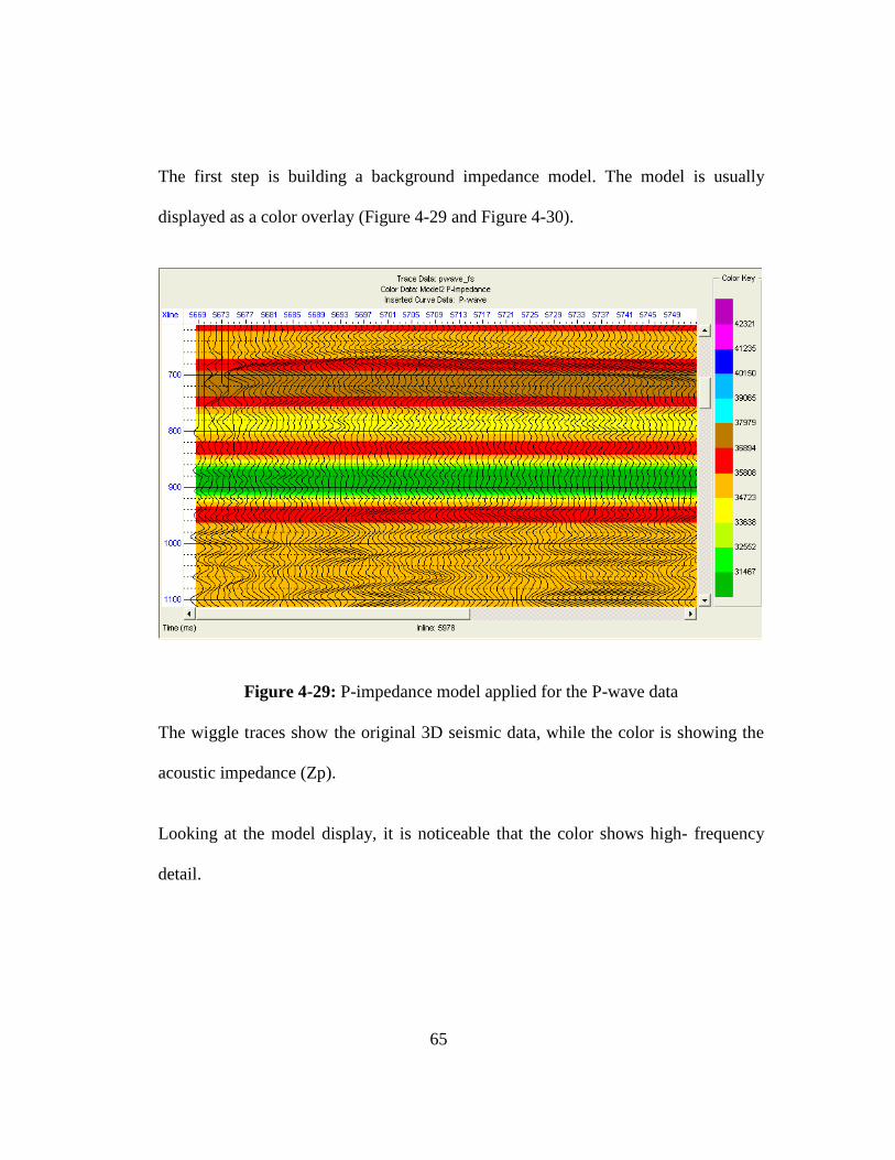
The first step is building a background impedance model. The model is usually
displayed as a color overlay (Figure 4-29 and Figure 4-30).
Figure 4-29: P-impedance model applied for the P-wave data
The wiggle traces show the original 3D seismic data, while the color is showing the
acoustic impedance (Zp).
Looking at the model display, it is noticeable that the color shows high- frequency
detail.
66
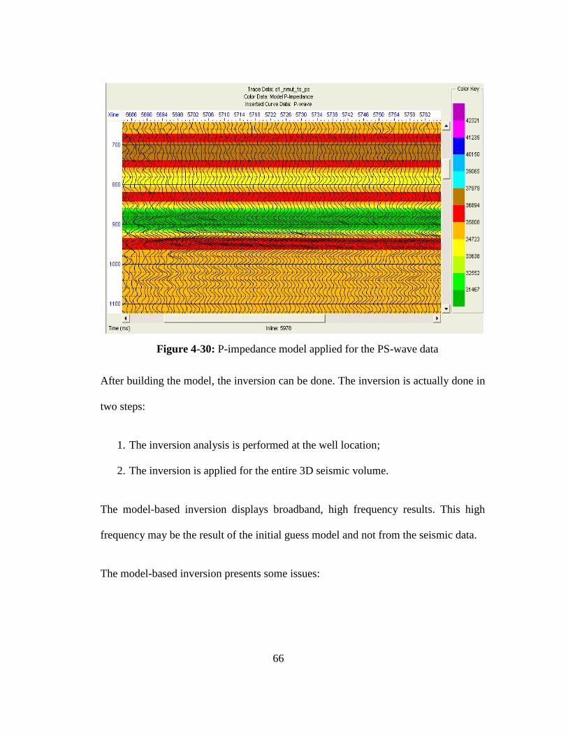
After building the model, the inversion can be done. The inversion is actually done in
two steps:
1. The inversion analysis is performed at the well location;
2. The inversion is applied for the entire 3D seismic volume.
The model-based inversion displays broadband, high frequency results. This high
frequency may be the result of the initial guess model and not from the seismic data.
The model-based inversion presents some issues:
Figure 4-30: P-impedance model applied for the PS-wave data
67
The effects of the wavelet are removed from the seismic through the
calculation;
Errors in the estimated wavelet will cause errors in the inversion result;
The effective resolution of the seismic is enhanced;
The result can be dependent on the initial guess model. This can be alleviated
by filtering the model;
There is a non-uniqueness problem, as with all inversion (Strata workshop).
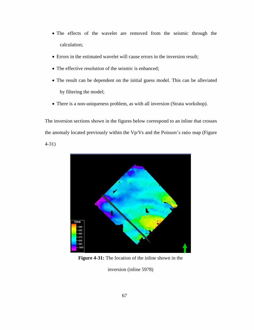
The inversion sections shown in the figures below correspond to an inline that crosses
the anomaly located previously within the Vp/Vs and the Poisson’s ratio map (Figure
4-31)
Figure 4-31: The location of the inline shown in the
inversion (inline 5978)
68
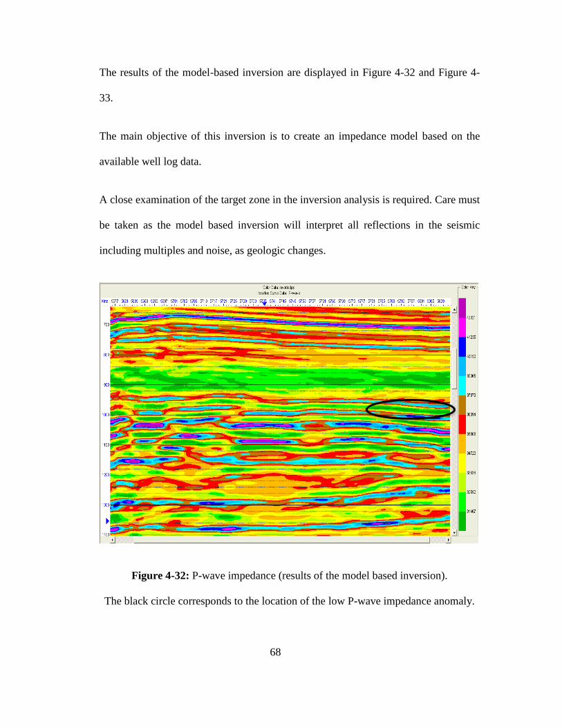
The results of the model-based inversion are displayed in Figure 4-32 and Figure 4-
33.
The main objective of this inversion is to create an impedance model based on the
available well log data.
A close examination of the target zone in the inversion analysis is required. Care must
be taken as the model based inversion will interpret all reflections in the seismic
including multiples and noise, as geologic changes.
Figure 4-32: P-wave impedance (results of the model based inversion).
The black circle corresponds to the location of the low P-wave impedance anomaly.
69
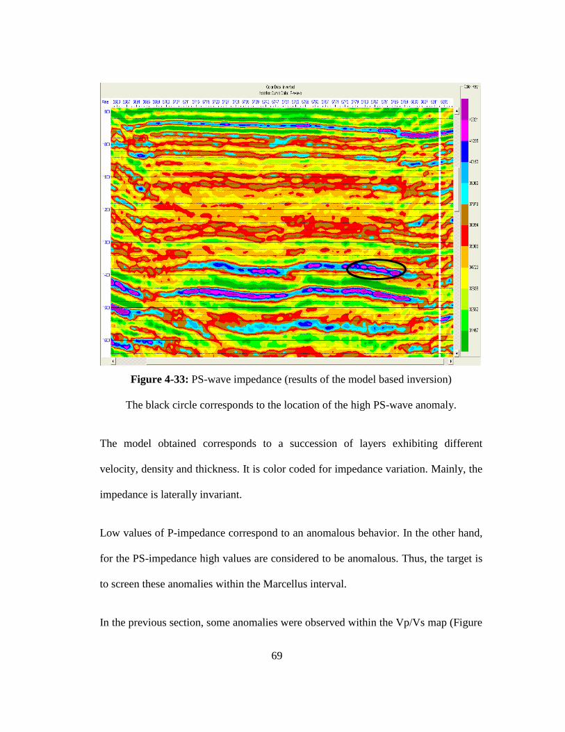
Figure 4-33: PS-wave impedance (results of the model based inversion)
The black circle corresponds to the location of the high PS-wave anomaly.
The model obtained corresponds to a succession of layers exhibiting different
velocity, density and thickness. It is color coded for impedance variation. Mainly, the
impedance is laterally invariant.
Low values of P-impedance correspond to an anomalous behavior. In the other hand,
for the PS-impedance high values are considered to be anomalous. Thus, the target is
to screen these anomalies within the Marcellus interval.
In the previous section, some anomalies were observed within the Vp/Vs map (Figure
70
4-13) as well as the Poisson’s ratio map (figure 4-14).
When analyzing the inversion results, the focus was the inversion sections that
correspond to the inlines and to the cross lines that cross the anomalies detected
previously.
The inversion results were encouraging as anomalous very low impedance regions,
dark green (circled in the P-impedance inversion figure), and very high impedance,
purple (circled in the PS-impedance inversion figure) were noticeable at the same
location of the anomalous low Vp/Vs and low Poisson’s ratio.
The seismic inversion delivered comparable results suggesting a good potential of the
possible sweet spots.
71
Chapter 5 Conclusion
The successful development of a shale gas depends upon the ability to understand a
number of key factors including understanding the brittleness distribution and the
location of the fractures.
Analysis of the Vp/Vs and the Poisson’s Ratio values from 3C-3D data in
combination with the inversion results reveal a good indicator of brittleness by
determining subtle lithological change, within the Marcellus. These results as well as
the results of the seismic attributes analysis can be used to refine drilling trajectories
and highlight potential targets.
The research confirms the applicability of Vp/Vs as a tool for exploration and
development of the Marcellus shale gas reservoir. However, all available data must be
included to avoid some misinterpretation consequence of erroneous Vp/Vs results.
The integration of all data, at all scales, leads to an understanding of the reservoir.
72
Chapter 6 Future work
The multicomponent seismic interpretation was achieved based on an image of one
well without having its exact location. Having more wells will improve and verify the
seismic interpretation for both seismic sections the compressional and the converted
wave data.
Core data could enhance the estimation of brittleness and better understand its
distribution.
Post-stack seismic inversion was generated from multicomponent seismic data based
on only one well. The results display the P-impedance volume. These results can be
improved and more accurate when using more well data. When more than one well is
entered into the model, the results are interpolated (by default) using inverse-distance
weighting.
The Vp/Vs was generated based on the multicomponent seismic traveltimes. The
Vp/Vs volume can also be estimated based on seismic inversion for impedance
according to the chart below (Figure 6-1). The two volumes can then be examined
carefully and compared to localize sweet spots or area within the two volumes
displaying a low Vp/Vs.
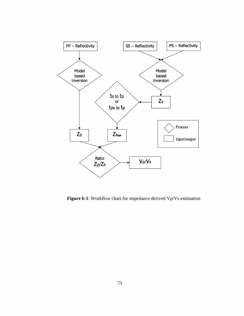
73
Figure 6-1: Workflow chart for impedance derived Vp/Vs estimation
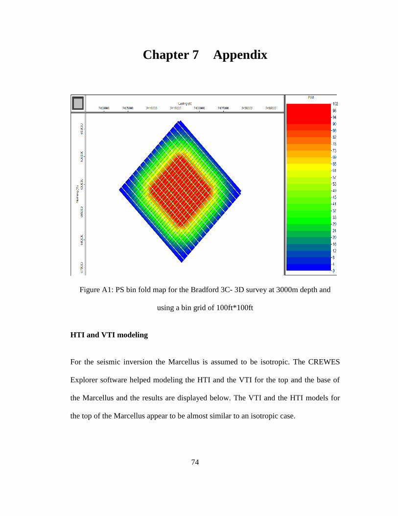
74
Chapter 7 Appendix
Figure A1: PS bin fold map for the Bradford 3C- 3D survey at 3000m depth and
using a bin grid of 100ft*100ft
HTI and VTI modeling
For the seismic inversion the Marcellus is assumed to be isotropic. The CREWES
Explorer software helped modeling the HTI and the VTI for the top and the base of
the Marcellus and the results are displayed below. The VTI and the HTI models for
the top of the Marcellus appear to be almost similar to an isotropic case.
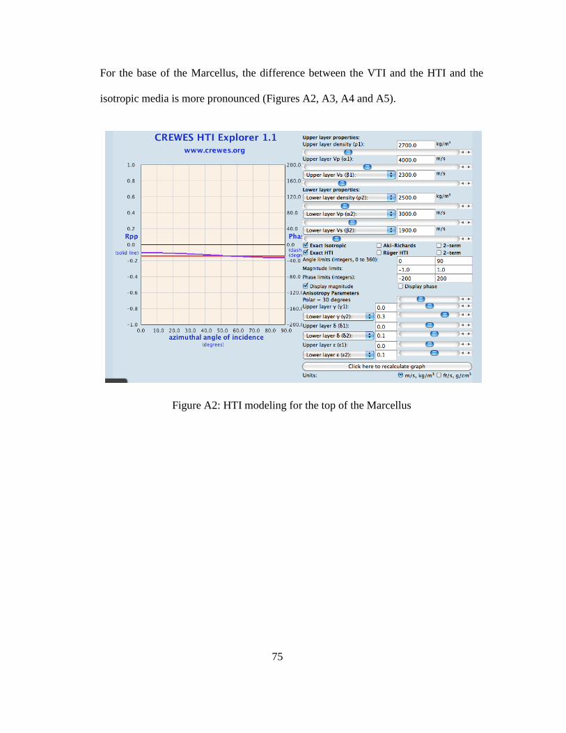
75
For the base of the Marcellus, the difference between the VTI and the HTI and the
isotropic media is more pronounced (Figures A2, A3, A4 and A5).
Figure A2: HTI modeling for the top of the Marcellus
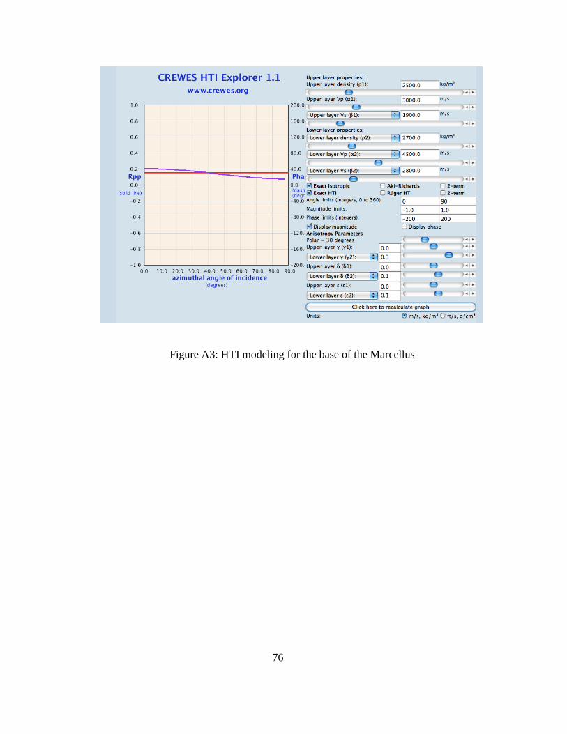
76
Figure A3: HTI modeling for the base of the Marcellus
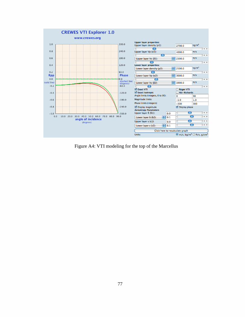
77
Figure A4: VTI modeling for the top of the Marcellus
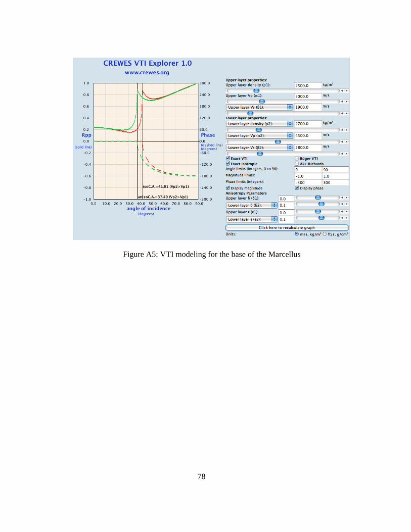
78
Figure A5: VTI modeling for the base of the Marcellus
79
Chapter 8 References
American Association of Petroleum Geologists, 2008, Distribution of Marcellus shale
in the Appalachian basin – a play that has industry analysts, operators and
observers all abuzz.
http://www.aapg.org/explorer/2008/03mar/marcellusDistribution.cfm.
Accessed August 9th
, 2012.
Ashton, C.P., B. Bacon., C. Deplante, and G. Redekop., 1994, 3D seismic survey
design. Oilfield review (April, 1994): 19-32.
Bircher, S. and G. Castillo., 2011, Integrated seismic approach to shale plays.
geomechanical properties and stress analysis from seismic data. CGG Veritas.
SEG San Antonio.
Bustin, R.M., A. Bustin., D. Ross, G. Chalmers, V. Murthy, C. Laxmi, and X. Cui.,
2009, Shale gas opportunities and challenges. AAPG, Search and Discovery.
Article #40382.
Chesapeake Energy., 2009, Northeast US Operations. 2009 AADE Mid Continent
Chapter Symposium.
Chesapeake Energy Corporation., 2012, Marcellus shale: New York, Pennsylvania,
West Virginia.
http://www.askchesapeake.com/MarcellusShale/Pages/Information.aspx.
Accessed September 21st 2011.
Chopra, S. and K.J. Marfurt., 2011, Interesting pursuits in seismic curvature attribute
80
analysis. CSEG recorder (April, 2011): 41-50.
Chopra, S. and K.J. Marfurt., 2005, Seismic attributes — A historical perspective.
Geophysics, 70 (5): 3SO–28SO.
Chuandong, X. and R.R. Stewart., 2004, Identifying channel sand versus shale using
3C-3D seismic data, VSPs and horizontal well logs. CREWES Project,
University of Calgary. SEG Int'l Exposition and 74th Annual Meeting.
Denver, Colorado.
Ciezobka, J., 2011, New Albany and Marcellus shale gas projects”. RPSEA
Unconventional Gas Conference 2011.
Cluff, B., 2009, Shale gas: opportunities and challenges for independents or, What’s
in it for me?. SIPES 2009 Annual Meeting, Hilton Head, S.C.
Common wealth of Pennsylvania, bureau of topographic and geologic survey. The
depositional setting of the marcellus black shale.
http://www.wvsoro.org/resources/marcellus/RamsayBarrett-Shale.pdf.
Accessed August 14th
2011.
Cordsen, A., 1995, How to find the optimum 3d fold. Annual Meeting of the
Canadian society of exploration geophysicists.
Core Lab, 2007, Shale reservoirs: Reservoir Characterization and Production
Optimization. www.corelab.com. Accessed Ocober 29th
2011.
Elmira, 2008, Gas well drilling and development Marcellus shale. Susquehanna River
Basin Commission meeting. June 12, New York.
Engelder, T. and G.G. Lash., 2008, Marcellus shale play’s vast resource potential
creating stir in Appalachia. The American oil and gas reporter.
81
http://www.aogr.com/index.php/magazine/cover-story/marcellus-shale-plays-
vast-resource-potential-creating-stir-in-appalachia. Accessed March, 2011.
Engelder, T., G.G. Lash. and R.S. Uzcátegui., 2009, Joint sets that enhance
production from Middle and Upper Devonian gas shales of the Appalachian
Basin”. AAPG Bulletin 93 (7): 857–889.
Gaiser, J., A. Chaveste., M. Edrich., T. Rebec and R. Verm., 2011, Seismic
anisotropy of the marcellus shale: feasibility study for fracture
characterization. Geokinetics Inc. Recovery. CSPG CSEG CWLS
Convention.
Gaiser, J.E., 2004, PS-wave azimuthal anisotropy: benefits for fractured reservoir.
AAPG, Search and Discovery. Article #40120.
Ganguly, N., D. Dearborn., M. Moore., D. Gordon., M. Horan, and S. Chopra., 2009,
Application of seismic curvature attribute in the appraisal of the Tishrine-
West field, North-East Syria. CSEG recorder (June 2009): 29-43.
Grieser, B., “Caney shale Oklahoma’s shale challenge”. Halliburton.
http://www.ogs.ou.edu/pdf/GSGrieserS.pdf. Accessed November, 3rd 2011.
Gretener, P., 2003, Summary of the Poisson’s ratio debate 1990 – 2003. CSEG
RECORDER. Feature article (September 2003): 44-45.
Grigor, S.R., 1998, Empirical relationships between anellipticity and Vp/Vs in shales:
Potential applications to AVO studies and anisotropic seismic processing.
SEG New Orleans.
Guliyev, E., 2007, vp/vs estimation from multicomponent seismic data for improved
characterization of a tight sandstone gas reservoir, rulison field, Colorado.
82
Master of Science, Golden, Colorado.
Hardage, B., M. deAngelo, and D. Sava., 2011, Marcellus shale geophysics. Bureau
of Economic Geology, UT Austin. RPSEA Meeting. April 20th
.
Hay, J., C.H, Sondergeld. Mechanical testing of shale by instrumented indentation.
Agilent technologies. http://nano.tm.agilent.com/nano_data_sheets/AN-
Shale_5990-5816.pdf. Accessed August, 9th
2012.
Hendrick, N., 2005, A preliminary evaluation of integrated P/PS seismic
interpretation for improved geological characterisation of coal environments.
Bowen Basin Symposium. Geophysics: 135-140.
Holmes, M., Holmes, D. and Holmes. A., 2011, A petrophysical model to estimate
free gas in organic shales. AAPG, Search and Discovery. Article #40781.
Koesoemadinata, A., 2011, Seismic reservoir characterization in Marcellus shale.
Shlumberger. SEG San Antonio.
Lash, G.G. and T. Engelder, 2011, Thickness trends and sequence stratigraphy of the
Middle Devonian Marcellus Formation, Appalachian Basin: Implications for
Acadian foreland basin evolution. AAPG Bulletin 95 (1): 61-103.
Legere, L., 2010, Marcellus shale production data exceeds expectations.
http://thetimes-tribune.com/news/marcellus-shale-production-data-exceeds-
expectations-1.1000300#axzz1obQfCOSZ. Accessed August 29th
2011.
Lewis, R., 2010, What makes a good gas shale?. Schlumberger, Oklahoma City.
Shale SPE TULSA.
Paddock, D., and C. Stolte., 2008, Seismic reservoir characterization of a gas shale
utilizing azimuthal data processing, pre-stack seismic inversion and ant
83
tracking. Schlumberger, SEG expanded abstract.
Paddock, D., 2012, 3D seismic profiles of U.S. shale plays. Schlumberger. AAPG E-
Symposium.
Prasad, M., A. Pal-Bathija., M. Johnston., M. Rydzy and M. Batzle., 2009, Rock
physics of the unconventional. The Leading Edge. January. Special section:
Rock Physics. 76: E117-E126
Rebec, T., J. Gaiser., A. Chaveste., M. Edrich., and R. Verm., 2011, The Marcellus
shale revealed with full azimuth 3D multi-component seismic data. AAPG,
Search and Discovery. Article #110160.
Roger M. S. and Y. Abousleiman., 2011, Multi-scale, brittle-ductile couplets in
unconventional gas shales: merging sequence stratigraphy and geomechanics.
AAPG, Search and Discovery. Article #80181.
Sayers, C.M., 1994, The elastic anisotrophy of shale. Journal of geophysical research,
99 (B1): 767-774.
Sondergeld, C.H., K.E. Newsham., J.T. Comisky, M.C. Rice, and C.S. Rai., 2010,
Petrophysical considerations in evaluating and producing shale gas resources.
SPE Unconventional Gas Conference, 23-25 Feb, Pittsburg Pennsylvania.
Sumi, L., 2008, Shale Gas: Focus on the Marcellus shale. Oil and Gas Accountability
Project, Earthworks. Schlumberger, Cambridge Research. SEG expanded
abstract