Processing and interpretation of 3D 3C seismic dta from an

Multicomponent interpretation

CREWES Research Report — Volume 27 (2015) 1

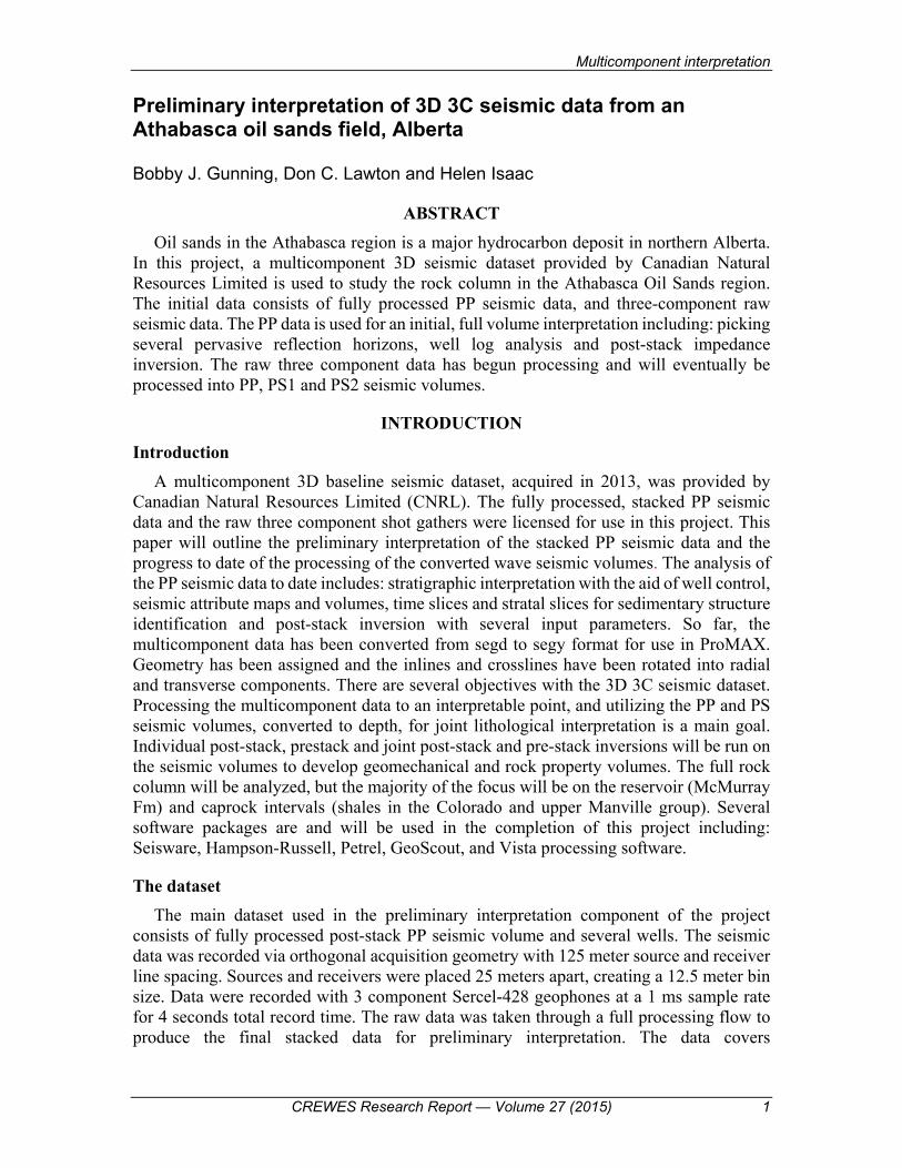
Preliminary interpretation of 3D 3C seismic data from an Athabasca oil sands field, Alberta

Bobby J. Gunning, Don C. Lawton and Helen Isaac

ABSTRACT Oil sands in the Athabasca region is a major hydrocarbon deposit in northern Alberta.

In this project, a multicomponent 3D seismic dataset provided by Canadian Natural Resources Limited is used to study the rock column in the Athabasca Oil Sands region. The initial data consists of fully processed PP seismic data, and three-component raw seismic data. The PP data is used for an initial, full volume interpretation including: picking several pervasive reflection horizons, well log analysis and post-stack impedance inversion. The raw three component data has begun processing and will eventually be processed into PP, PS1 and PS2 seismic volumes.

INTRODUCTION Introduction

A multicomponent 3D baseline seismic dataset, acquired in 2013, was provided by Canadian Natural Resources Limited (CNRL). The fully processed, stacked PP seismic data and the raw three component shot gathers were licensed for use in this project. This paper will outline the preliminary interpretation of the stacked PP seismic data and the progress to date of the processing of the converted wave seismic volumes. The analysis of the PP seismic data to date includes: stratigraphic interpretation with the aid of well control, seismic attribute maps and volumes, time slices and stratal slices for sedimentary structure identification and post-stack inversion with several input parameters. So far, the multicomponent data has been converted from segd to segy format for use in ProMAX. Geometry has been assigned and the inlines and crosslines have been rotated into radial and transverse components. There are several objectives with the 3D 3C seismic dataset. Processing the multicomponent data to an interpretable point, and utilizing the PP and PS seismic volumes, converted to depth, for joint lithological interpretation is a main goal. Individual post-stack, prestack and joint post-stack and pre-stack inversions will be run on the seismic volumes to develop geomechanical and rock property volumes. The full rock column will be analyzed, but the majority of the focus will be on the reservoir (McMurray Fm) and caprock intervals (shales in the Colorado and upper Manville group). Several software packages are and will be used in the completion of this project including: Seisware, Hampson-Russell, Petrel, GeoScout, and Vista processing software.

The dataset The main dataset used in the preliminary interpretation component of the project

consists of fully processed post-stack PP seismic volume and several wells. The seismic data was recorded via orthogonal acquisition geometry with 125 meter source and receiver line spacing. Sources and receivers were placed 25 meters apart, creating a 12.5 meter bin size. Data were recorded with 3 component Sercel-428 geophones at a 1 ms sample rate for 4 seconds total record time. The raw data was taken through a full processing flow to produce the final stacked data for preliminary interpretation. The data covers

Gunning, Lawton, and Isaac

2 CREWES Research Report — Volume 27 (2015)

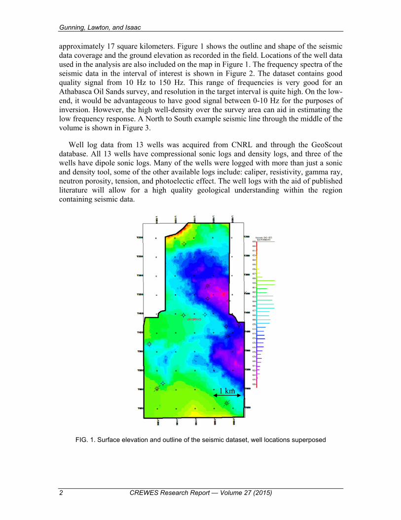
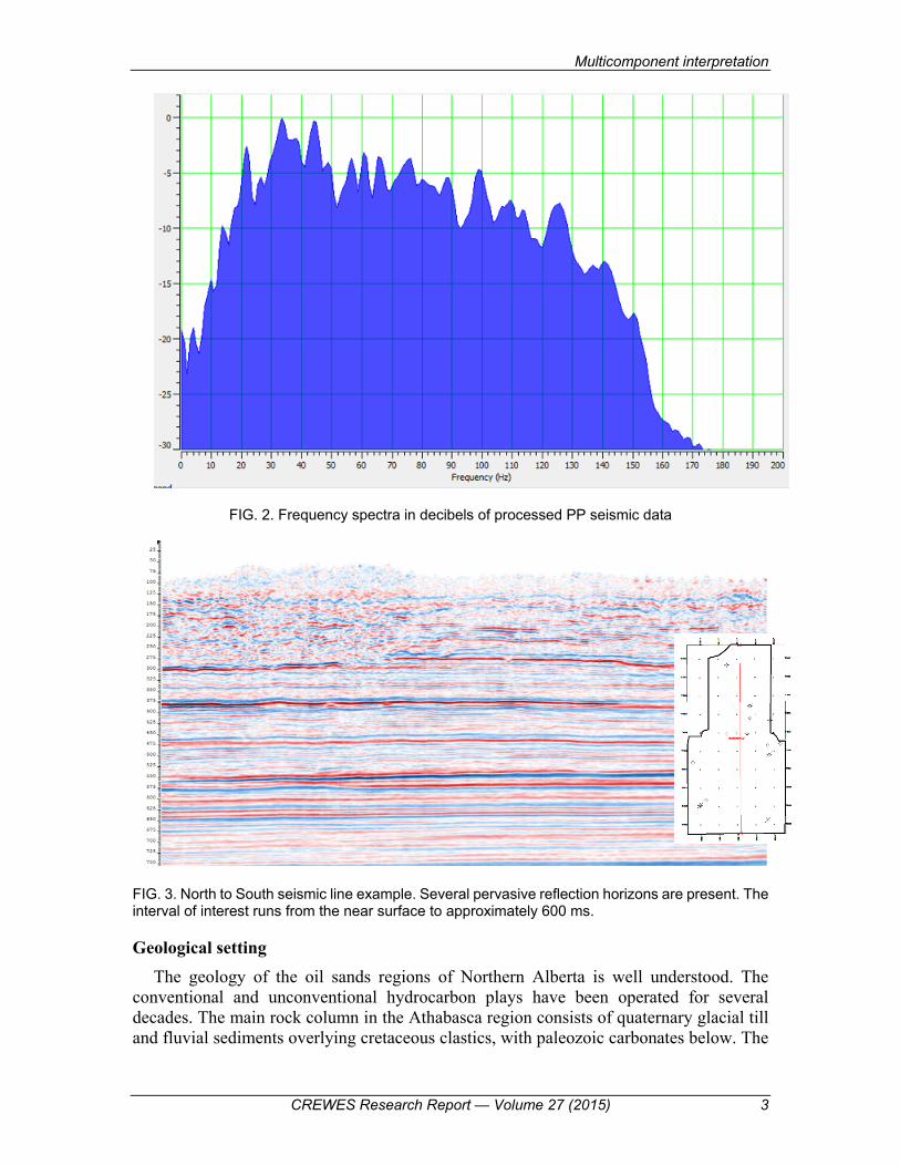
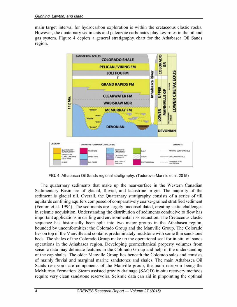
approximately 17 square kilometers. Figure 1 shows the outline and shape of the seismic data coverage and the ground elevation as recorded in the field. Locations of the well data used in the analysis are also included on the map in Figure 1. The frequency spectra of the seismic data in the interval of interest is shown in Figure 2. The dataset contains good quality signal from 10 Hz to 150 Hz. This range of frequencies is very good for an Athabasca Oil Sands survey, and resolution in the target interval is quite high. On the low-end, it would be advantageous to have good signal between 0-10 Hz for the purposes of inversion. However, the high well-density over the survey area can aid in estimating the low frequency response. A North to South example seismic line through the middle of the volume is shown in Figure 3.

Well log data from 13 wells was acquired from CNRL and through the GeoScout database. All 13 wells have compressional sonic logs and density logs, and three of the wells have dipole sonic logs. Many of the wells were logged with more than just a sonic and density tool, some of the other available logs include: caliper, resistivity, gamma ray, neutron porosity, tension, and photoelectic effect. The well logs with the aid of published literature will allow for a high quality geological understanding within the region containing seismic data.

FIG. 1. Surface elevation and outline of the seismic dataset, well locations superposed

1 km



FIG. 2. Frequency spectra in decibels of processed PP seismic data

FIG. 3. North to South seismic line example. Several pervasive reflection horizons are present. The interval of interest runs from the near surface to approximately 600 ms.

Geological setting The geology of the oil sands regions of Northern Alberta is well understood. The

conventional and unconventional hydrocarbon plays have been operated for several decades. The main rock column in the Athabasca region consists of quaternary glacial till and fluvial sediments overlying cretaceous clastics, with paleozoic carbonates below. The



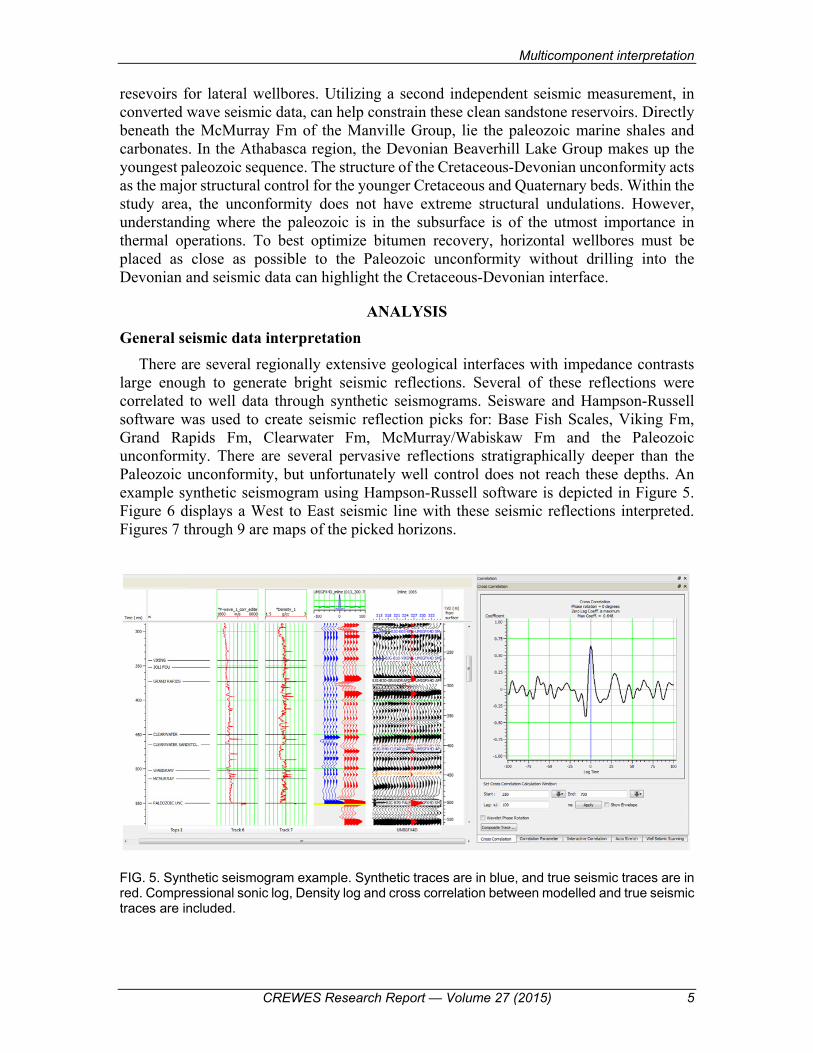
main target interval for hydrocarbon exploration is within the cretaceous clastic rocks. However, the quaternary sediments and paleozoic carbonates play key roles in the oil and gas system. Figure 4 depicts a general stratigraphy chart for the Athabasca Oil Sands region.

FIG. 4: Athabasca Oil Sands regional stratigraphy. (Todorovic-Marinic et al. 2015)

The quaternary sediments that make up the near-surface in the Western Canadian Sedimentary Basin are of glacial, fluvial, and lacustrine origin. The majority of the sediment is glacial till. Overall, the Quaternary stratigraphy consists of a series of till aquitards confining aquifers composed of comparatively coarse-grained stratified sediment (Fenton et al. 1994). The sediments are largely unconsolidated, creating static challenges in seismic acquisition. Understanding the distribution of sediments conducive to flow has important applications in drilling and environmental risk reduction. The Cretaceous clastic sequence has historically been split into two major groups in the Athabasca region, bounded by unconformities: the Colorado Group and the Manville Group. The Colorado lies on top of the Manville and contains predominately mudstone with some thin sandstone beds. The shales of the Colorado Group make up the operational seal for in-situ oil sands operations in the Athabasca region. Developing geomechanical property volumes from seismic data may deliniate features in the Colorado Group and help in the understanding of the cap shales. The older Manville Group lies beneath the Colorado sales and consists of mainly fluvial and marginal marine sandstones and shales. The main Athabasca Oil Sands reservoirs are components of the Manville group, the main reservoir being the McMurray Formation. Steam assisted gravity drainage (SAGD) in-situ recovery methods require very clean sandstone reservoirs. Seismic data can aid in pinpointing the optimal



resevoirs for lateral wellbores. Utilizing a second independent seismic measurement, in converted wave seismic data, can help constrain these clean sandstone reservoirs. Directly beneath the McMurray Fm of the Manville Group, lie the paleozoic marine shales and carbonates. In the Athabasca region, the Devonian Beaverhill Lake Group makes up the youngest paleozoic sequence. The structure of the Cretaceous-Devonian unconformity acts as the major structural control for the younger Cretaceous and Quaternary beds. Within the study area, the unconformity does not have extreme structural undulations. However, understanding where the paleozoic is in the subsurface is of the utmost importance in thermal operations. To best optimize bitumen recovery, horizontal wellbores must be placed as close as possible to the Paleozoic unconformity without drilling into the Devonian and seismic data can highlight the Cretaceous-Devonian interface.

ANALYSIS General seismic data interpretation

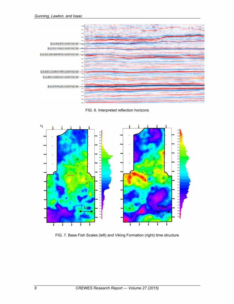
There are several regionally extensive geological interfaces with impedance contrasts large enough to generate bright seismic reflections. Several of these reflections were correlated to well data through synthetic seismograms. Seisware and Hampson-Russell software was used to create seismic reflection picks for: Base Fish Scales, Viking Fm, Grand Rapids Fm, Clearwater Fm, McMurray/Wabiskaw Fm and the Paleozoic unconformity. There are several pervasive reflections stratigraphically deeper than the Paleozoic unconformity, but unfortunately well control does not reach these depths. An example synthetic seismogram using Hampson-Russell software is depicted in Figure 5. Figure 6 displays a West to East seismic line with these seismic reflections interpreted. Figures 7 through 9 are maps of the picked horizons.

FIG. 5. Synthetic seismogram example. Synthetic traces are in blue, and true seismic traces are in red. Compressional sonic log, Density log and cross correlation between modelled and true seismic traces are included.



FIG. 6. Interpreted reflection horizons

FIG. 7. Base Fish Scales (left) and Viking Formation (right) time structure

1 km 1 km



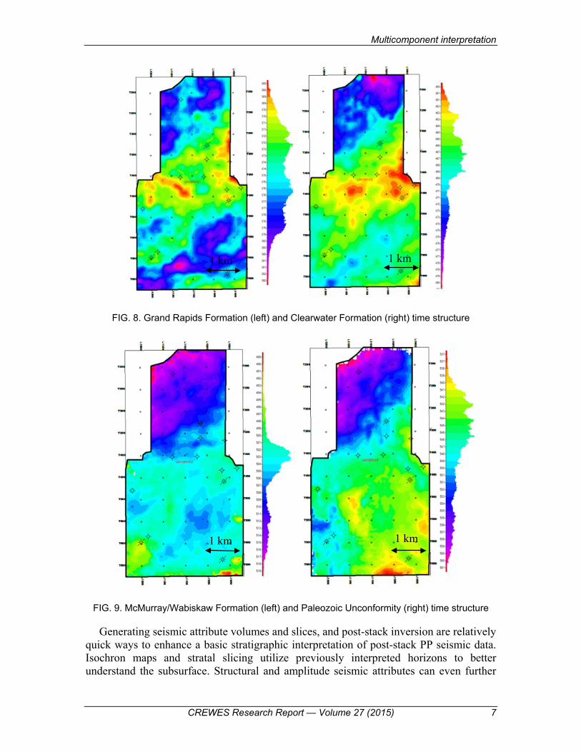
FIG. 8. Grand Rapids Formation (left) and Clearwater Formation (right) time structure

FIG. 9. McMurray/Wabiskaw Formation (left) and Paleozoic Unconformity (right) time structure

Generating seismic attribute volumes and slices, and post-stack inversion are relatively quick ways to enhance a basic stratigraphic interpretation of post-stack PP seismic data. Isochron maps and stratal slicing utilize previously interpreted horizons to better understand the subsurface. Structural and amplitude seismic attributes can even further

1 km 1 km

1 km 1 km



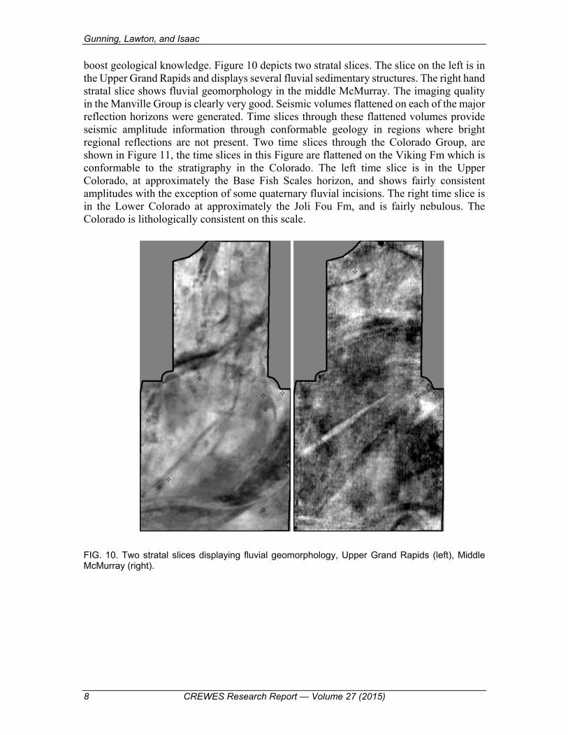
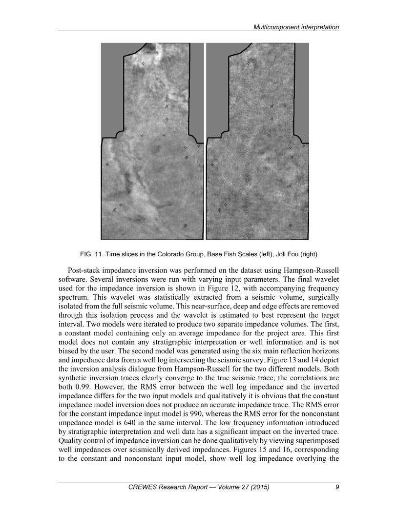
boost geological knowledge. Figure 10 depicts two stratal slices. The slice on the left is in the Upper Grand Rapids and displays several fluvial sedimentary structures. The right hand stratal slice shows fluvial geomorphology in the middle McMurray. The imaging quality in the Manville Group is clearly very good. Seismic volumes flattened on each of the major reflection horizons were generated. Time slices through these flattened volumes provide seismic amplitude information through conformable geology in regions where bright regional reflections are not present. Two time slices through the Colorado Group, are shown in Figure 11, the time slices in this Figure are flattened on the Viking Fm which is conformable to the stratigraphy in the Colorado. The left time slice is in the Upper Colorado, at approximately the Base Fish Scales horizon, and shows fairly consistent amplitudes with the exception of some quaternary fluvial incisions. The right time slice is in the Lower Colorado at approximately the Joli Fou Fm, and is fairly nebulous. The Colorado is lithologically consistent on this scale.

FIG. 10. Two stratal slices displaying fluvial geomorphology, Upper Grand Rapids (left), Middle McMurray (right).



FIG. 11. Time slices in the Colorado Group, Base Fish Scales (left), Joli Fou (right)

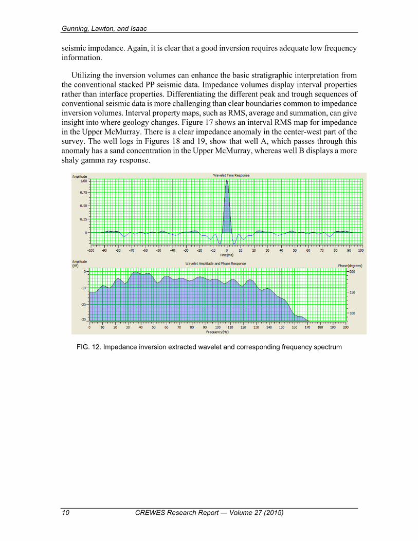
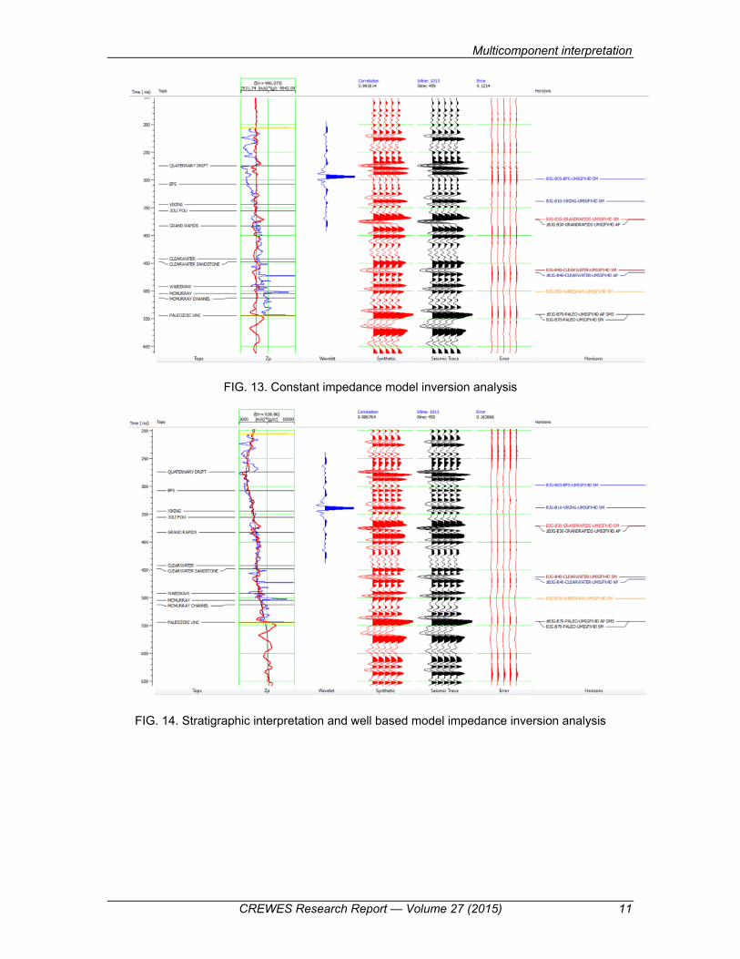
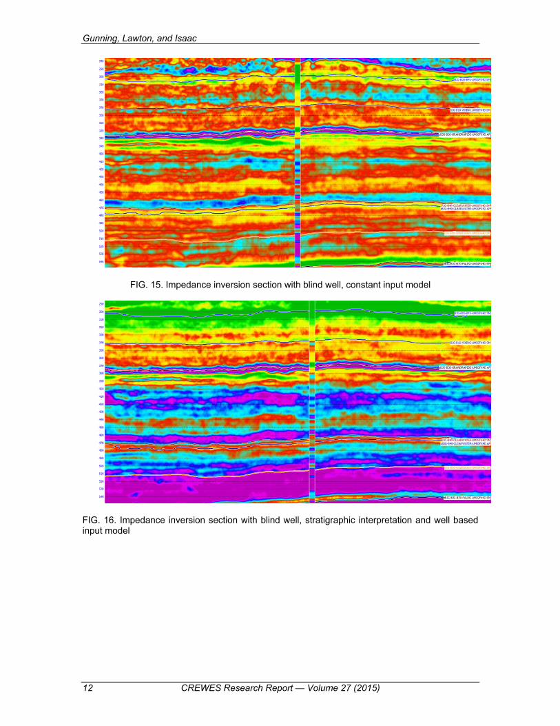
Post-stack impedance inversion was performed on the dataset using Hampson-Russell software. Several inversions were run with varying input parameters. The final wavelet used for the impedance inversion is shown in Figure 12, with accompanying frequency spectrum. This wavelet was statistically extracted from a seismic volume, surgically isolated from the full seismic volume. This near-surface, deep and edge effects are removed through this isolation process and the wavelet is estimated to best represent the target interval. Two models were iterated to produce two separate impedance volumes. The first, a constant model containing only an average impedance for the project area. This first model does not contain any stratigraphic interpretation or well information and is not biased by the user. The second model was generated using the six main reflection horizons and impedance data from a well log intersecting the seismic survey. Figure 13 and 14 depict the inversion analysis dialogue from Hampson-Russell for the two different models. Both synthetic inversion traces clearly converge to the true seismic trace; the correlations are both 0.99. However, the RMS error between the well log impedance and the inverted impedance differs for the two input models and qualitatively it is obvious that the constant impedance model inversion does not produce an accurate impedance trace. The RMS error for the constant impedance input model is 990, whereas the RMS error for the nonconstant impedance model is 640 in the same interval. The low frequency information introduced by stratigraphic interpretation and well data has a significant impact on the inverted trace. Quality control of impedance inversion can be done qualitatively by viewing superimposed well impedances over seismically derived impedances. Figures 15 and 16, corresponding to the constant and nonconstant input model, show well log impedance overlying the



seismic impedance. Again, it is clear that a good inversion requires adequate low frequency information.

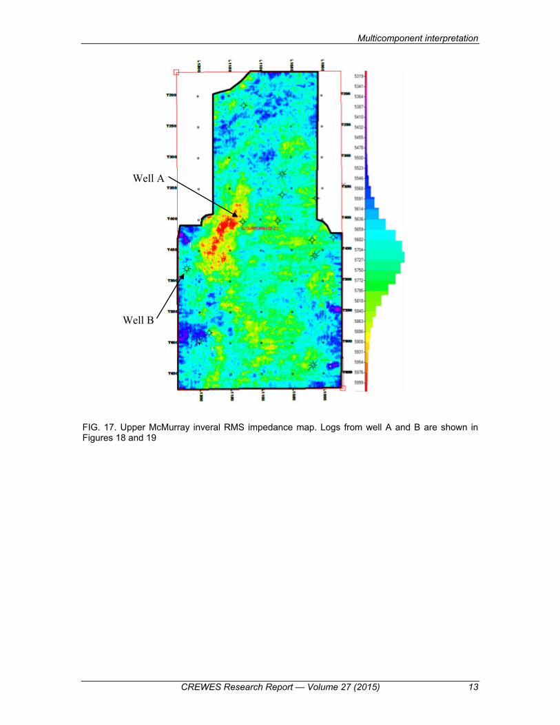
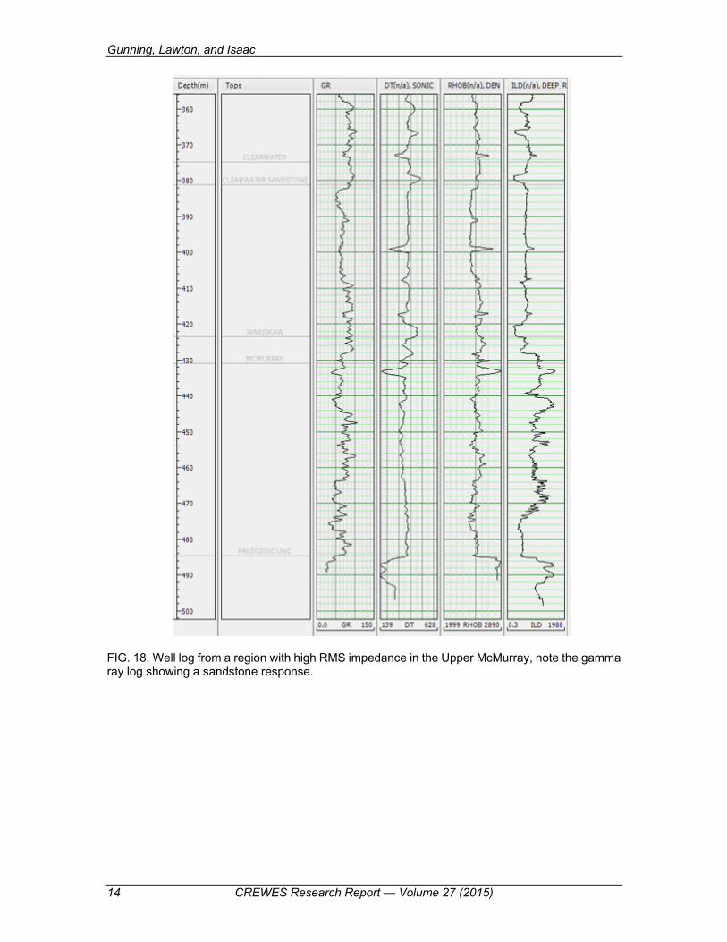
Utilizing the inversion volumes can enhance the basic stratigraphic interpretation from the conventional stacked PP seismic data. Impedance volumes display interval properties rather than interface properties. Differentiating the different peak and trough sequences of conventional seismic data is more challenging than clear boundaries common to impedance inversion volumes. Interval property maps, such as RMS, average and summation, can give insight into where geology changes. Figure 17 shows an interval RMS map for impedance in the Upper McMurray. There is a clear impedance anomaly in the center-west part of the survey. The well logs in Figures 18 and 19, show that well A, which passes through this anomaly has a sand concentration in the Upper McMurray, whereas well B displays a more shaly gamma ray response.

FIG. 12. Impedance inversion extracted wavelet and corresponding frequency spectrum



FIG. 13. Constant impedance model inversion analysis

FIG. 14. Stratigraphic interpretation and well based model impedance inversion analysis



FIG. 15. Impedance inversion section with blind well, constant input model

FIG. 16. Impedance inversion section with blind well, stratigraphic interpretation and well based input model



FIG. 17. Upper McMurray inveral RMS impedance map. Logs from well A and B are shown in Figures 18 and 19

Well A

Well B



FIG. 18. Well log from a region with high RMS impedance in the Upper McMurray, note the gamma ray log showing a sandstone response.



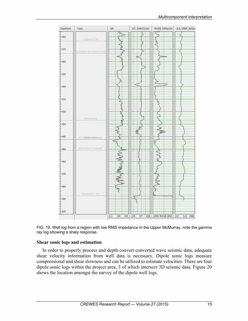
FIG. 19. Well log from a region with low RMS impedance in the Upper McMurray, note the gamma ray log showing a shaly response.

Shear sonic logs and estimation In order to properly process and depth convert converted wave seismic data, adequate

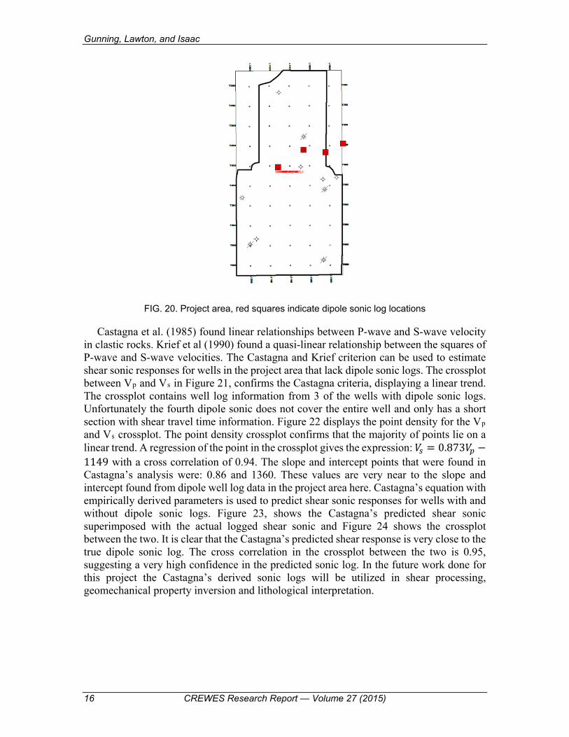
shear velocity information from well data is necessary. Dipole sonic logs measure compressional and shear slowness and can be utilized to estimate velocities. There are four dipole sonic logs within the project area, 3 of which intersect 3D seismic data. Figure 20 shows the location amongst the survey of the dipole well logs.



FIG. 20. Project area, red squares indicate dipole sonic log locations

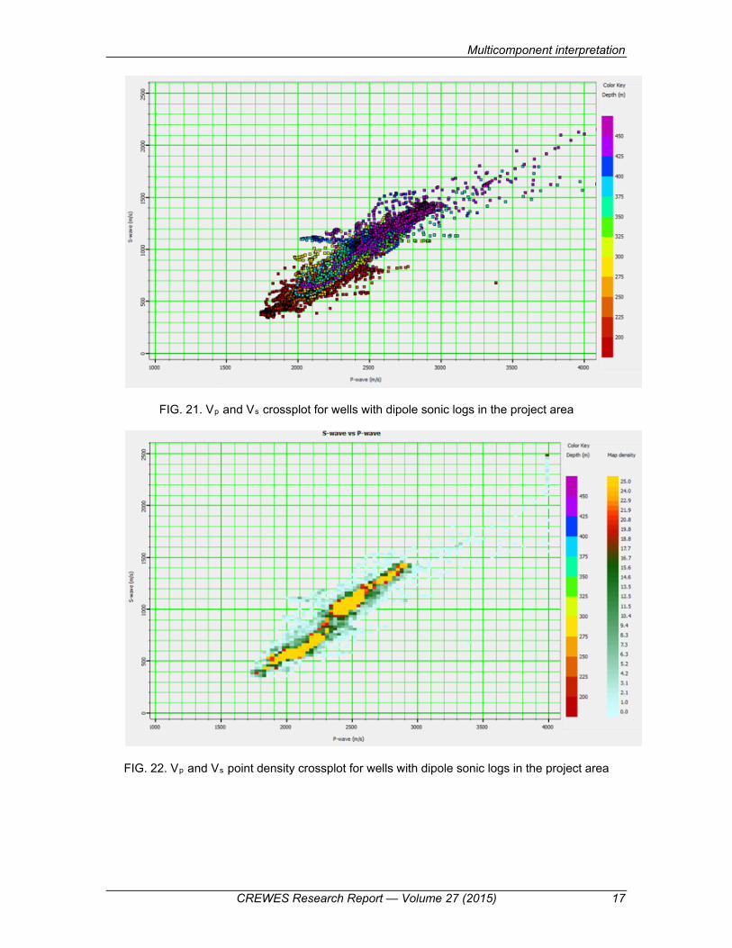
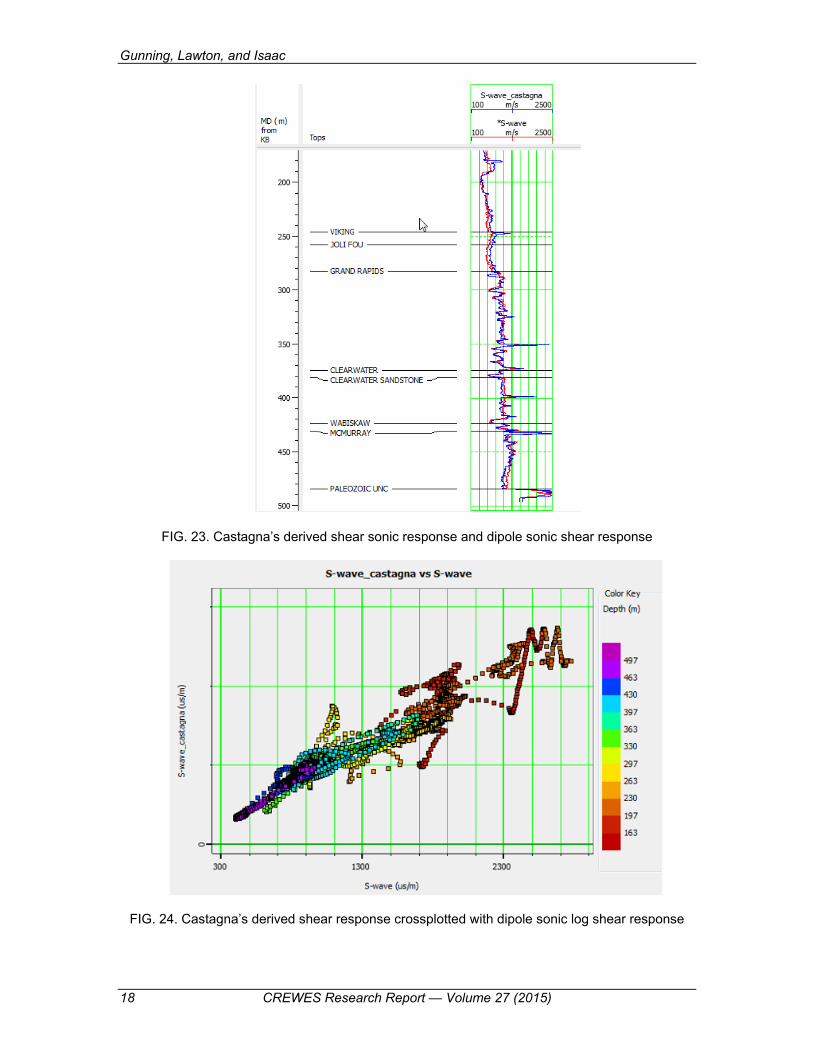
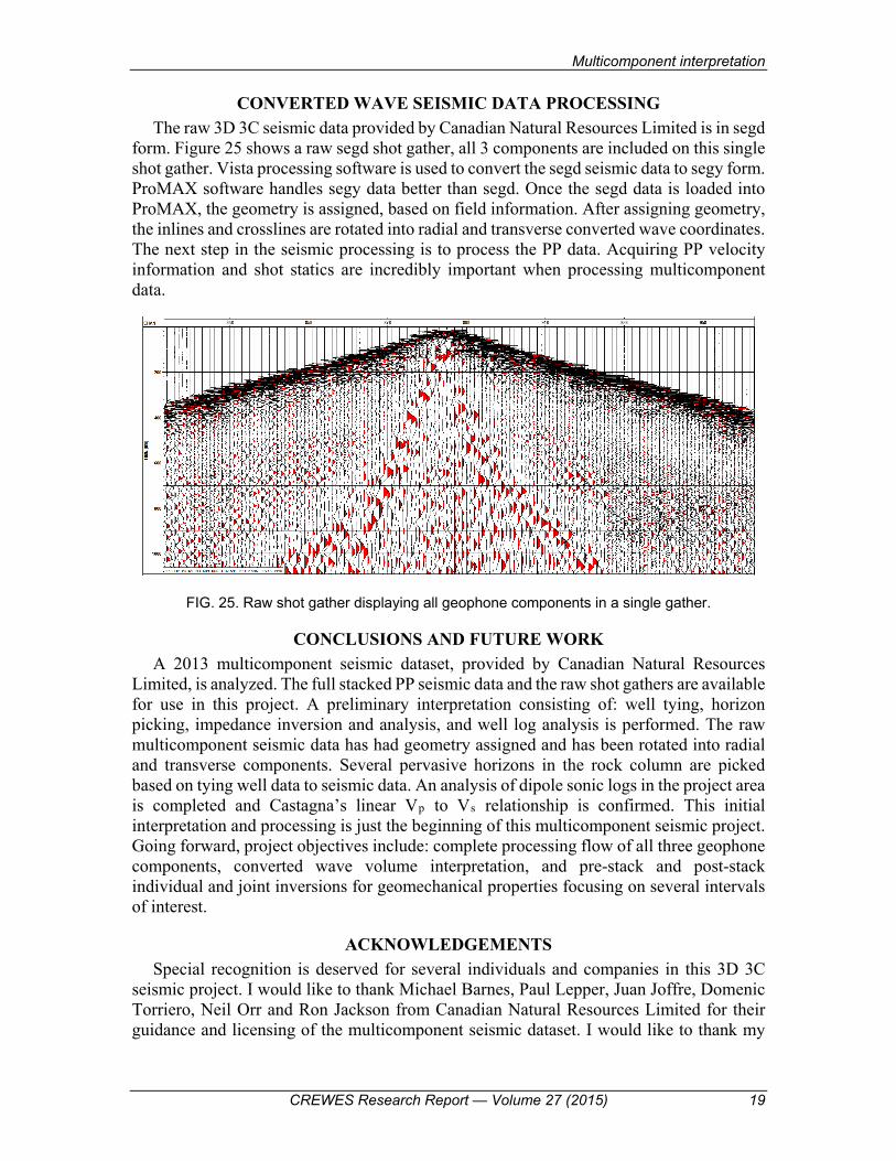
Castagna et al. (1985) found linear relationships between P-wave and S-wave velocity in clastic rocks. Krief et al (1990) found a quasi-linear relationship between the squares of P-wave and S-wave velocities. The Castagna and Krief criterion can be used to estimate shear sonic responses for wells in the project area that lack dipole sonic logs. The crossplot between Vp and Vs in Figure 21, confirms the Castagna criteria, displaying a linear trend. The crossplot contains well log information from 3 of the wells with dipole sonic logs. Unfortunately the fourth dipole sonic does not cover the entire well and only has a short section with shear travel time information. Figure 22 displays the point density for the Vp and Vs crossplot. The point density crossplot confirms that the majority of points lie on a linear trend. A regression of the point in the crossplot gives the expression: 𝑉𝑉𝑠𝑠 = 0.873𝑉𝑉𝑝𝑝 −1149 with a cross correlation of 0.94. The slope and intercept points that were found in Castagna’s analysis were: 0.86 and 1360. These values are very near to the slope and intercept found from dipole well log data in the project area here. Castagna’s equation with empirically derived parameters is used to predict shear sonic responses for wells with and without dipole sonic logs. Figure 23, shows the Castagna’s predicted shear sonic superimposed with the actual logged shear sonic and Figure 24 shows the crossplot between the two. It is clear that the Castagna’s predicted shear response is very close to the true dipole sonic log. The cross correlation in the crossplot between the two is 0.95, suggesting a very high confidence in the predicted sonic log. In the future work done for this project the Castagna’s derived sonic logs will be utilized in shear processing, geomechanical property inversion and lithological interpretation.



FIG. 21. Vp and Vs crossplot for wells with dipole sonic logs in the project area

FIG. 22. Vp and Vs point density crossplot for wells with dipole sonic logs in the project area



FIG. 23. Castagna’s derived shear sonic response and dipole sonic shear response

FIG. 24. Castagna’s derived shear response crossplotted with dipole sonic log shear response



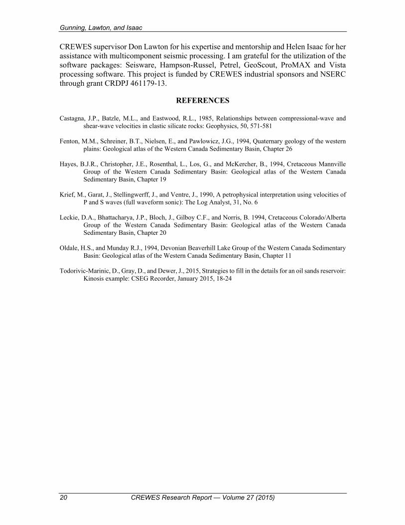
CONVERTED WAVE SEISMIC DATA PROCESSING The raw 3D 3C seismic data provided by Canadian Natural Resources Limited is in segd

form. Figure 25 shows a raw segd shot gather, all 3 components are included on this single shot gather. Vista processing software is used to convert the segd seismic data to segy form. ProMAX software handles segy data better than segd. Once the segd data is loaded into ProMAX, the geometry is assigned, based on field information. After assigning geometry, the inlines and crosslines are rotated into radial and transverse converted wave coordinates. The next step in the seismic processing is to process the PP data. Acquiring PP velocity information and shot statics are incredibly important when processing multicomponent data.

FIG. 25. Raw shot gather displaying all geophone components in a single gather.

CONCLUSIONS AND FUTURE WORK A 2013 multicomponent seismic dataset, provided by Canadian Natural Resources

Limited, is analyzed. The full stacked PP seismic data and the raw shot gathers are available for use in this project. A preliminary interpretation consisting of: well tying, horizon picking, impedance inversion and analysis, and well log analysis is performed. The raw multicomponent seismic data has had geometry assigned and has been rotated into radial and transverse components. Several pervasive horizons in the rock column are picked based on tying well data to seismic data. An analysis of dipole sonic logs in the project area is completed and Castagna’s linear Vp to Vs relationship is confirmed. This initial interpretation and processing is just the beginning of this multicomponent seismic project. Going forward, project objectives include: complete processing flow of all three geophone components, converted wave volume interpretation, and pre-stack and post-stack individual and joint inversions for geomechanical properties focusing on several intervals of interest.

ACKNOWLEDGEMENTS Special recognition is deserved for several individuals and companies in this 3D 3C

seismic project. I would like to thank Michael Barnes, Paul Lepper, Juan Joffre, Domenic Torriero, Neil Orr and Ron Jackson from Canadian Natural Resources Limited for their guidance and licensing of the multicomponent seismic dataset. I would like to thank my



CREWES supervisor Don Lawton for his expertise and mentorship and Helen Isaac for her assistance with multicomponent seismic processing. I am grateful for the utilization of the software packages: Seisware, Hampson-Russel, Petrel, GeoScout, ProMAX and Vista processing software. This project is funded by CREWES industrial sponsors and NSERC through grant CRDPJ 461179-13.

REFERENCES Castagna, J.P., Batzle, M.L., and Eastwood, R.L., 1985, Relationships between compressional-wave and shear-wave velocities in clastic silicate rocks: Geophysics, 50, 571-581 Fenton, M.M., Schreiner, B.T., Nielsen, E., and Pawlowicz, J.G., 1994, Quaternary geology of the western plains: Geological atlas of the Western Canada Sedimentary Basin, Chapter 26 Hayes, B.J.R., Christopher, J.E., Rosenthal, L., Los, G., and McKercher, B., 1994, Cretaceous Mannville Group of the Western Canada Sedimentary Basin: Geological atlas of the Western Canada Sedimentary Basin, Chapter 19 Krief, M., Garat, J., Stellingwerff, J., and Ventre, J., 1990, A petrophysical interpretation using velocities of P and S waves (full waveform sonic): The Log Analyst, 31, No. 6 Leckie, D.A., Bhattacharya, J.P., Bloch, J., Gilboy C.F., and Norris, B. 1994, Cretaceous Colorado/Alberta Group of the Western Canada Sedimentary Basin: Geological atlas of the Western Canada Sedimentary Basin, Chapter 20 Oldale, H.S., and Munday R.J., 1994, Devonian Beaverhill Lake Group of the Western Canada Sedimentary Basin: Geological atlas of the Western Canada Sedimentary Basin, Chapter 11 Todorivic-Marinic, D., Gray, D., and Dewer, J., 2015, Strategies to fill in the details for an oil sands reservoir: Kinosis example: CSEG Recorder, January 2015, 18-24

Documents

Processing and interpretation of 3D 3C seismic dta from an